Maturity Structure and Debt Renegotiation in SovereignBonds

Taghi Farzad ∗

University of California, Riverside

Abstract

This paper develops a model of endogenous default with debt renegotiation foremerging economies. A small open economy faces a stochastic stream of income. Thegovernment can issue short and long term bonds and makes decision on behalf of theresidents of the borrowing country. Lenders are risk-neutral and operate in a perfectlycompetitive financial market. Upon default, the borrowing country loses access to thefinancial markets and will not be able to borrow any longer. The defaulted countryhas to pay off the principal and interest of the restructured debt to regain access tothe credit market. Debt restructuring is modeled by a Nash bargaining game. Theresulted equilibrium haircut is directly related to the debt level. This feature results ina default value function that flattens out after an endogenous threshold; consequentlydefault happens at higher debt levels compared to models without debt renegotiation.The model is calibrated to capture the default episodes in Argentina. The proposedmodel has several advantages over extant literature. First, the model statistics closelymatch the observed values. This is particularly the case for the resulted interest ratedistributions for short and long term bonds, compared to previous literature. Providinga precise interest rate distribution is crucial as finding the optimal maturity structurerelies on it. Furthermore, interest rates can be an indicative of financial crisis. Thepaper finds that endogenous debt renegotiation is an important mechanism in gener-ating more realistic fluctuations of the interest rate. The proposed model can be usedas a policy tool to predict and understand dynamics of financial crises related to debtdefault.

Keywords: Sovereign Default, Sovereign Bonds, Maturity Structure, Debt Renegotiation∗taghi.farzad@email.ucr.edu.

The latest version can be found on https://sites.google.com/view/taghifarzad/home/research.

1

1 Introduction

Recurrence of financial crises and prolonged debt settlement process in emerg-ing countries induce questions regarding the role of debt structure in sovereigndefault. Thus, debt maturity composition and its impact on the interest ratedraw a lot of research attention. It is well-documented fact that the interestrate plays an important role in emerging economies.1 Hence, it is crucial toinvestigate the reciprocal effect of debt maturity structure and the interestrate spreads faced by an emerging economy. In particular, Broner, Lorenzoni,and Schmukler (2013) show that for emerging economies short term debts aregenerally cheaper than long term debts. Due to an increase in dilution risks,2

the long term borrowing is even costlier near financial crises. As a result,countries will shorten the maturity composition in the imminence of a finan-cial crisis. This implies that while long term borrowing is expensive, thesovereign government suffers massively from rolling over the short term debtnear default episodes.

This paper provides a default model with two debt instruments, short andlong term bonds, and endogenous debt renegotiation. A risk averse sovereignfaces a stream of income and issues bonds that will be traded in a perfectlycompetitive market with risk neutral lenders. Contingent on the state ofthe economy depending on income shocks and short and long term debts,sovereign may find it optimal to default. 3 Lenders determine the price ofa bond taking into account these default probabilities. Upon default, an en-dogenous haircut will be applied to the short and long term bonds. Adding

1See Neumeyer and Perri (2005), Aguiar and Gopinath (2006)2Dilution risk can be defined as the capital loss for the current long term lenders after issuance of new

bonds. While both short and long term bonds are affected by the default risk, only the latter is impacted bythe dilution risk.

3This paper does not consider the possibility of partial defaults.

2

the endogenous debt renegotiation feature to the model allows us to furtherstudy the dilution risk.

This paper is closely related to a set of previous studies. Arellano and Ra-manarayanan (2012) proposed a similar model but with no recovery, i.e. 100%haircut. Hatchondo, Martinez, and Sosa-Padilla (2016) proposed a modelwith exogenous debt dilution that was constant over the states. Bi (2006)applies Yue (2010) renegotiation approach to one- and two-period bonds,representing short and long term bonds, respectively. This paper improvesBi’s (2006) approach by allowing the country to issue bonds with longer ma-turities. in order to achieve this, we model bonds as perpetuity contractswith non-state-contingent payments that decay at a constant rate.4 As inMacaulay (1938), different decay rates can represent bonds with different du-rations. This allows us to circumvent the curse of dimensionality and studythe effect of bonds with longer maturities. Bi (2006) assumes the recoveryrate is a function of the total outstanding debt.5 In this paper, the state-contingent debt is a function of the income and of short and long term debts,instead of total debt. We find that expressing the recovery rate as a functionof total debt is a specific case of our model when the sovereign is forced topay the arrears in one period. We conclude that this can lead to suboptimaldecision policies.

As explained in Bi (2006), interest rate and debt dilution are the mainfactors affecting default episodes. Most of the papers that extend Eaton and

4see e.g. Arellano and Ramanarayanan 2012, Hatchondo et al. 2016, and Hatchondo and Martinez 2009.5As discussed in Farzad (2018a), when the sovereign issues one-period bonds and loans, the recovery rate

is a function of total debt. However, in presence of bonds with different maturity, this approach relies on thepresumption that upon default the total debt will be repaid in one period. The default episodes are morelikely when the income realization is low and, assuming income persistence, the income is likely to remainlow in the future periods. This means the country that is forced to pay back the debt in one period suffersmassively from default. This process may artificially reduce the default incentives.

3

Gersovitz (1981) address the effect of endogenously determined interest rate.The effect of debt dilution is either discarded (Arellano 2008, Arellano and Ra-manarayanan 2012) or modeled by a constant exogenous factor (Hatchondo etal. 2016). This paper models the renegotiation using Nash Bargaining game,as in Yue (2010) and Bi (2006). As in Bi (2006) and Farzad (2018a), the mainfocus of the proposed model is on pari passu debt contracts; all outstandingdebts are treated equally upon default. Hence, the same haircut is applied toshort and long term debts. Bi (2006) argues how lenders tend to hold shortterm bonds near the default to prevent the debt dilution. Hatchondo et al.(2016) show that without debt dilution the optimal maturity of debt increasesby 2 years. Hence, it is crucial to take into account the effect of debt dilutionin addition to the interest rate impacts.

We calibrate the model to the Argentina data. We find that the model pre-dictions are closely related to patterns in the data. In particular, the spreaddynamics match the observed data: The spread curves (difference betweenthe interest rate of a maturity and corresponding risk free interest rate) areupwards sloping during tranquil times, but flatten out or even invert closerto financial crisis. We show that the proposed model with endogenous debtrenegotiation delivers spread distribution closer to data compared to modelswith either no recovery rate or an exogenous one. In short, the equilibriumendogenous recovery rate allows the borrowing country to hold higher levelsof debt before declaring a default. Consequently, the observed interest ratesare higher than the models without debt renegotiation. At the onset of cri-sis, the debt dilution effect reduces the long term bond prices more than theprice of the short term bonds. Hence borrowing countries shorten the matu-rity composition. Issuing short term bonds increases the default probability

4

but does not affect the debt dilution risk. This results in an even larger shortterm spread. Studying the behavior of interest rates as done in this paperis important for two main reasons. First, high interest rates are leading in-dicators of financial crisis. Second, finding the optimal maturity depends ofanalyzing the interest dynamics for different maturities. The proposed modelcan be used as an important policy tool to predict and understand dynamicsof financial crises related to debt default.

Literature Review

This paper is related to several strands of research. It builds on seminal workof Eaton and Gersovitz (1981) that developed an endogenous default model.This paper also emphasizes on the role of (endogenous) interest rate in finan-cial crisis. This is in line with Neumeyer and Perri (2005) conclusion thatinterest rate spread is an important factor in explaining the business cyclefluctuations in emerging economies. As indicated by Aguiar and Gopinath(2006) models with one-period bonds are not capable of fully capturing thespread fluctuations. Arellano (2008) shows increasing the default cost in amodel with one-period bonds can induce higher spreads. To generate a posi-tive spread,even when the economy is not exposed to a high default probabil-ity, researchers added debts with longer maturities: Even in tranquil times,sovereign is exposed to a “bad” income shock over the span of a long termdebt that may lead to a default episode. Taking into account this unpleasantdraw, long term lenders will charge a higher interest rate. Chatterjee and Eyi-gungor (2008), improved Arellano’s (2008) approach by letting the sovereignto issue bonds with longer maturities. The results provide a better fit for thespread behavior in emerging economies.

Broner et al. (2013) studied the effect of debt maturity composition in

5

emerging economies. They document that the risk premium on long termdebts is relatively higher, and would increase during crisis. This shifts thedebt issuance toward short term debts. To explain this fact, Arellano and Ra-manarayanan (2008) and Hatchondo and Martinez (2009) developed modelsthat include both short and long term bonds. The long term bonds are rep-resented by perpetuity payments with a decay rate. As in Macaulay (1938),finite durations can be modeled with a proper decay rate.6 This allows usto develop a model in which debt maturity can be changed by a choosinganother decay rate.

Hatchondo et al. (2016) and Bi (2006) improved the previous works bystudying the debt dilution effects. Hatchondo et al. (2016) use a constantexogenous recovery rate that is applied to defaulted debts. Bi (2006) appliesthe Nash Bargaining (a la Yue 2010) to find the endogenous recovery ratesfor one and two period bonds. Bulow and Rogoff (1989) proposed a modelwith Rubinstein’s (1982) type of bargaining in the debt rescheduling process.As discussed by Bi (2006), not only the Nash Bargaining approach is moretractable, but it also delivers results that can be supported by Rubinsteingame or other complicated game structures.7

Sturzenegger and Zettelmeyer (2008) show the inter-creditor equity wasex-post violated for many of the debt restructuring between 1998 and 2005.This is mainly due to higher post-exchange yields, that result in a lower NPVfor higher maturity debts. Since there is not enough evidence in favor of ex-ante discrimination, Hatchondo et al. (2016), Bi (2006), and Farzad (2018a)all assume the same debt recovery rate for different debt instruments. This is

6Hatchondo and Martinez (2009) explain this approach is used in empirical studies as well as credit ratingagencies.

7For instance see Bai and Zhang (2009) for the application of stochastic bargaining model.

6

based on the assumption of pari passu debts. Collective action clauses (CACs)and comparability of treatment (in Paris Club principals) can further justifyapplying the same haircut to short and long term bonds.8 Due to the lackof legally-binding rules regarding the seniority of debts, we do not considerpriorities in debt repayment.

The outline of the paper is as follows: Section 2 provides the theoreticalmodel. Section 3 presents the theoretical results and propositions for thepaper. Section 4 contains the quantitative analysis for the model, and finallysection 5 concludes the paper.

2 Model

Time is discrete and is indexed by t ∈ {0, 1, . . . }. The economy faces a streamof income {y1, y2, . . . yn} that follows a Markov process with transition matrixf(yt+1|yt). There is a representative agent that lives forever, with preferencesrepresented by

E0∞∑t=0

βtu(ct)

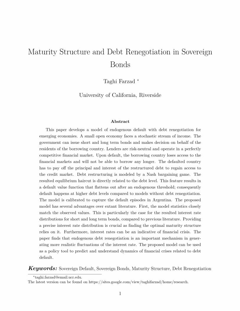
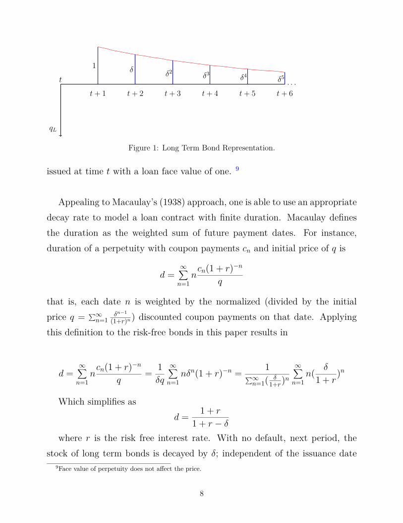
where 0 < β < 1 is the discount factor. Later we assume u is a CARA util-ity function, hence it is continuous, strictly increasing, and strictly concave.Each period, a benevolent sovereign decides on the level of consumption andborrowings. Government can issue either short term, BS, or long term, BL,bonds. Short term bond is a one-period bond sold at the discount price qSand delivers the face value next period. Long term bond, as in Arellano andRamanarayanan (2012) and Hatchondo and Martinez (2009), is modeled by aperpetuity contract with coupon payments that decay geometrically. Figure1 depicts the payments associated with the perpetuity contract of a bond

8See Das et al (2012) and Farzad (2018a)

7

t+ 1 t+ 2 t+ 3 t+ 4 t+ 5 t+ 6t

1δ

δ2δ3

δ4δ5

qL

. . .

Figure 1: Long Term Bond Representation.

issued at time t with a loan face value of one. 9

Appealing to Macaulay’s (1938) approach, one is able to use an appropriatedecay rate to model a loan contract with finite duration. Macaulay definesthe duration as the weighted sum of future payment dates. For instance,duration of a perpetuity with coupon payments cn and initial price of q is

d =∞∑n=1

ncn(1 + r)−n

q

that is, each date n is weighted by the normalized (divided by the initialprice q = ∑∞

n=1δn−1

(1+r)n ) discounted coupon payments on that date. Applyingthis definition to the risk-free bonds in this paper results in

d =∞∑n=1

ncn(1 + r)−n

q= 1δq

∞∑n=1

nδn(1 + r)−n = 1∑∞n=1( δ

1+r)n∞∑n=1

n( δ

1 + r)n

Which simplifies asd = 1 + r

1 + r − δwhere r is the risk free interest rate. With no default, next period, the

stock of long term bonds is decayed by δ; independent of the issuance date9Face value of perpetuity does not affect the price.

8

each bond is decayed by the factor of δ. In addition, sovereign’s borrowing(lending) this period will add to (subtract from) next period’s stock of thebonds. Hence the law of motion for stock of long term bonds can be definedas

BL,t+1 = δBL,t + lt

where lt is current period’s issuance or repayment of long term bonds.10

The price of new issued bonds, either short or long term, depends on thesovereign’s state;

qSt (BS,t+1, BL,t+1, yt), qLt (BS,t+1, BL,t+1, yt).

Borrowing Country

There is a benevolent government that makes decision regarding consumptionand the issuance (or repayment) of short and long term bonds. At a givenstate (BS, BL, y), a sovereign has an option to either service the debt and getthe value of W (BS, BL, y) or default and get V D(BS, BL, y) . The value ofthe sovereign, V (BS, BL, y), is the maximum of these two:

V (BS, BL, y) = max{W (BS, BL, y), V D(BS, BL, y)

}

Contingent on honoring the debt, current consumption and new issuance(repayment) of each type of bonds will be determined according to the fol-lowing problem:

W (BS, BL, y) = maxB′S , B′L, 0≤C

u(C) + β∫YV (B′S, B′L, y′)f(y′|y)dy′

10For the one period bonds, δ is zero; hence, the stock of short term bonds will be the same as the amountissued (or bought) in the current period.

9

s.t. C +BS +BL = y + qS(B′S, B′L, y)B′S + qL(B′S, B′L, y)l′L

B′L = δBL + l′L

Defaulted sovereign will be excluded from the capital market, hence only willbe able to consume the current income. The arrears consist of the principaland the due interest. Contingent on the state of the economy, a haircut 1−αwill be applied to the outstanding short term and long term debt levels.

V D(BS, BL, y) = u(y) + β{ ∫

YWD(α(1 + r)BS, α(1 + r)BL, y

′)f(y′|y)dy′}

We can assume the country has the option of permanently leaving the creditmarket. However with the assumptions on the utility function and the param-eters used in these paper, it is never optimal to do so. Direct output loss, λ,and lacking a smoothed consumption profile make the Autarky a suboptimalchoice.

V AUT (y) = u((1− λ)y) + β∫YV AUT (y′)dµ(y′|y)

Following Yue (2010), it is assumed that the sovereign will regain access tothe credit market after paying the arrears in full. Until then, defaulted countryhas to (weakly) decrease short and long term debts, 0 ≤ B′S ≤ BS, 0 ≤ B′L ≤BL. Since the country is a net lender, the discount price for short and long

10

term bonds will be the corresponding risk-free interest rate:

WD(BS, BL, y) = max0≤B′S≤BS , 0≤B′L≤BL, 0≤C

u(C) + β∫YWD(B′S, B′L, y′)f(y′|y)dy′

C +BS +BL = (1− λ)y + B′S1 + r

+ l′L1 + r − δ

B′L = δBL + l′L

(1)

When the arrears are fully paid, the sovereign will regain access to the creditmarket and will be able to issue new bonds:

WD(0, 0, y) = V (0, 0, y)

Debt Renegotiation Problem

BSt is issued

t− 1 t t+ 1

Default α(1 + r)BSt

PVt−1 = α(·)(1 + r)BSt

(1 + r)2 = α(·)BSt

(1 + r)

BLt is issued

t− 1 t t+ 1 t+ 2

Default α(1 + r)BLt × 1 α(1 + r)BL

t × δ. . .

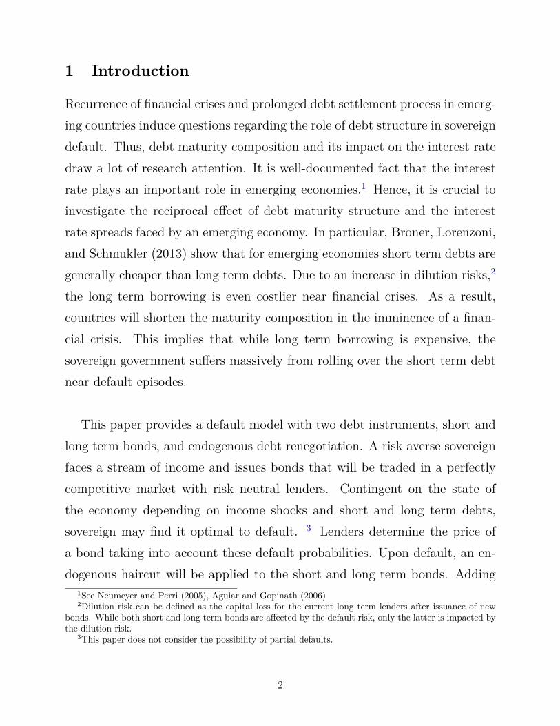
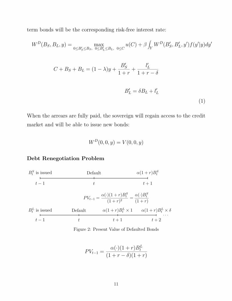
Figure 2: Present Value of Defaulted Bonds

PVt−1 = α(·)(1 + r)BLt

(1 + r − δ)(1 + r)

11

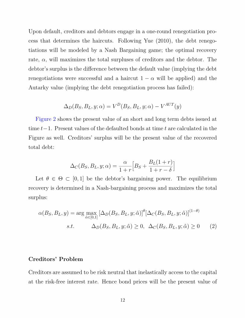
Upon default, creditors and debtors engage in a one-round renegotiation pro-cess that determines the haircuts. Following Yue (2010), the debt renego-tiations will be modeled by a Nash Bargaining game; the optimal recoveryrate, α, will maximizes the total surpluses of creditors and the debtor. Thedebtor’s surplus is the difference between the default value (implying the debtrenegotiations were successful and a haircut 1 − α will be applied) and theAutarky value (implying the debt renegotiation process has failed):

∆D(BS, BL, y;α) = V D(BS, BL, y;α)− V AUT (y)

Figure 2 shows the present value of an short and long term debts issued attime t−1. Present values of the defaulted bonds at time t are calculated in theFigure as well. Creditors’ surplus will be the present value of the recoveredtotal debt:

∆C(BS, BL, y;α) = α

1 + r

[BS + BL(1 + r)

1 + r − δ

]

Let θ ∈ Θ ⊂ [0, 1] be the debtor’s bargaining power. The equilibriumrecovery is determined in a Nash-bargaining process and maximizes the totalsurplus:

α(BS, BL, y) = arg maxα∈[0,1]

[∆D(BS, BL, y; α)]θ[∆C(BS, BL, y; α)](1−θ)

s.t. ∆D(BS, BL, y; α) ≥ 0, ∆C(BS, BL, y; α) ≥ 0 (2)

Creditors’ Problem

Creditors are assumed to be risk neutral that inelastically access to the capitalat the risk-free interest rate. Hence bond prices will be the present value of

12

the expected future payments. Assume the short and long term debt areBS and BL, respectively. Following Arellano and Ramanarayanan (2012), letR(BS, BL) denote the set of output levels at which the country services thedebt, and D(BS, BL) the set of output levels at which default is optimal:

R(BS, BL) = {y : W (BS, BL, y) ≥ V D(BS, BL, y)}

D(BS, BL) = {y : W (BS, BL, y) < V D(BS, BL, y)} (3)

One-period bonds are expected to pay back the face value if the sovereignhoners the debt, and the recovered value (α fraction of the face value) if thesovereign defaults. Hence, one can write the price of the one-period bond as:

qS,t =∫

R(bSt+1,bLt+1)

f(yt+1, yt)(1 + r) dyt+1 +

∫D(bSt+1,b

Lt+1)

α(bSt+1, bLt+1, yt+1)

f(yt+1, yt)(1 + r) dyt+1

(4)

For the long term bonds, contingent on servicing the debt till n periodsahead, the present value of the period t+n to creditor is δn−1

(1+r)n . The countrymay defaults in period t + n, contingent of servicing the debt in periodst+ 1, t+ 2, . . . , t+ n− 1. Upon default, it is expected to receive α fraction ofthe the outstanding debt δn−1 1+r

1+r−δ . Notice this paper assumes after default,the sovereign has to pay back all the outstanding debts before issuing newbonds. This implies countries cannot default twice on the same bond.

13

qLt =∞∑n=1

δn−1

(1 + r)n ∫R(bSt+1,b

Lt+1)

. . .∫

R(bSt+n,bLt+n)

f(yt+n, yt+m−1) . . . f(yt + 1, yt)dyt+n . . . dyt+1

+∞∑n=1

δn−1

(1 + r)n∫

R(bSt+1,bLt+1)

. . .∫

D(bSt+n,bLt+n)

α(bSt+n, bLt+n, yt+n)1 + r

1 + r − δ

f(yt+n, yt+n−1) . . . f(yt + 1, yt)dyt+n . . . dyt+1

As in Arellano and Ramanarayanan(2012), one can write the above ex-pression in a recursive form:

qLt =∫

R(bSt+1,bLt+1)

f(yt+1, yt)(1 + r) dyt+1 +

∫D(bSt+1,b

Lt+1)

α(bSt+1, bLt+1, yt+1)

1 + r

1 + r − δf(yt+1, yt)

(1 + r) dyt+1

+δ∫

R(bSt+1,bLt+1)

[ ∫R(bSt+2,b

Lt+2)

f(yt+2, yt+1)(1 + r)2 dyt+2

]f(yt+1, yt)dyt+1

+δ∫

R(bSt+1,bLt+1)

[ ∫D(bSt+2,b

Lt+2)

(1 + r)α(bSt+2, bLt+2, yt+2)

1 + r − δf(yt+2, yt+1)

(1 + r)2 dyt+2

]f(yt+1, yt)dyt+1

+ . . .

14

since the expression in the brackets is qLt+1, the the price function reduces to:

qLt = 11 + r

{ ∫R(bSt+1,b

Lt+1)

[1 + δqLt+1(bSt+2, b

Lt+2, yt+1)

]f(yt+1, yt)dyt+1

+∫

D(bSt+1,bLt+1)

1 + r

1 + r − δα(bSt+1, b

Lt+1, yt+1)f(yt+1, yt)dyt+1

}

(5)

For δ = 0, this will reduce to the price of the short term bond, expressedin 5. With 100% haircuts, the above expression will be reduced to Arellanoand Ramanarayanan (2012). Furthermore, with α = 1 for all the states, thelong term bond will turn to a risk-free bond:

(1 + r)qL =∫

R(bSt+1,bLt+1)

1 + δqLt+1(bSt+1, bLt+1, yt+1)f(yt+1, yt)dyt+1

+∫

D(bSt+1,bLt+1)

1 + r

1 + r − δf(yt+1, yt)dyt+1

+∫

R(bSt+1,bLt+1)

1 + r

1 + r − δf(yt+1, yt)dyt+1 −

∫R(bSt+1,b

Lt+1)

1 + r

1 + r − δf(yt+1, yt)dyt+1

(1 + r − δ

∫R(bSt+1,b

Lt+1)

f(yt+1, yt)dyt+1

)qL =

(1 + r − δ

∫R(bSt+1,b

Lt+1)

f(yt+1, yt)dyt+1

) 11 + r − δ

qL = 11 + r − δ

15

3 Results

Recursive Equilibrium

A recursive equilibrium for this economy consists of a set of functions definedbelow; for s = (BS, BL, y):

• The country’s value functions, V (s),W (s), V D(s),WD(s), and V (y)AUT

and policy functions of short and long term bonds, B′S(s), B′L(s), andconsumption, C(s),

• Default set, D(BS, BL), and the repayment set R(BS, BL),

• Price functions qS(B′S, B′L, y) and qL(B′S, B′L, y) in 4 and 5, such thatgiven the recovery rate α(s)

1. The default and the repayment sets are the equilibrium sets definedabove,

2. Next period’s bond holdings are in agreement with the country’spolicy functions:

bSt+1 = B′S(s), bLt+1 = B′L(s)

• The recovery rate function α(s) such that

1. Given the bond prices and the recovery rate, country solves the recursiveproblem

2. Given the bond prices, the value functions, the policy functions, and thedefault and repayment sets, recovery rate solves the debt renegotiationproblem.

3. Given the recovery rate, bond prices satisfy the zero profit condition forthe bondholders.

16

Proposition 1: ∀θ ∈ Θ recursive equilibrium of the above model exist.

Lemma 1: The debt renegotiation problem is invariant to any transfer ofdebt that keeps BS + BL(1+r)

1+r−δ unchanged.

Proof : See Appendix

Proposition 2: The equilibrium recovery rate, α(BS, BL, y), satisfies

α(BS, BL, y) =

1 (BS + dδBL) ≤ ζ(y)

ζ(y)(BS+dδBL) (BS + dδBL) ≥ ζ(y)

(6)

where dδ = 1+r1+r−δ .

Proof : See Appendix

This result extends Yue (2010) to two dimensions and Farzad (2018a) toinstruments with different maturities.11 Upon default, for each level of endow-ment y, the value function of default is independent of BS +dδBL, henceforthcalled the total dated debt. This simplification helps us to derive the sameset of result as in Eaton and Gersovitz (1981) and Chatterjee et al. (2007),Arellano (2008), Yue (2010), and Bi (2006) all explained below.

11for one period debt instruments, δ = 0, the relation reduces to BS +BL, as in Farzad (2018a).

17

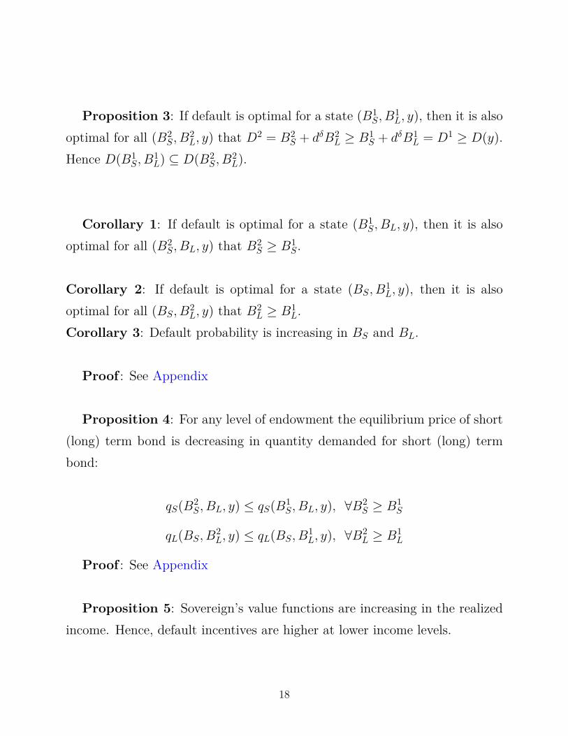
Proposition 3: If default is optimal for a state (B1S, B

1L, y), then it is also

optimal for all (B2S, B

2L, y) that D2 = B2

S + dδB2L ≥ B1

S + dδB1L = D1 ≥ D(y).

Hence D(B1S, B

1L) ⊆ D(B2

S, B2L).

Corollary 1: If default is optimal for a state (B1S, BL, y), then it is also

optimal for all (B2S, BL, y) that B2

S ≥ B1S.

Corollary 2: If default is optimal for a state (BS, B1L, y), then it is also

optimal for all (BS, B2L, y) that B2

L ≥ B1L.

Corollary 3: Default probability is increasing in BS and BL.

Proof : See Appendix

Proposition 4: For any level of endowment the equilibrium price of short(long) term bond is decreasing in quantity demanded for short (long) termbond:

qS(B2S, BL, y) ≤ qS(B1

S, BL, y), ∀B2S ≥ B1

S

qL(BS, B2L, y) ≤ qL(BS, B

1L, y), ∀B2

L ≥ B1L

Proof : See Appendix

Proposition 5: Sovereign’s value functions are increasing in the realizedincome. Hence, default incentives are higher at lower income levels.

18

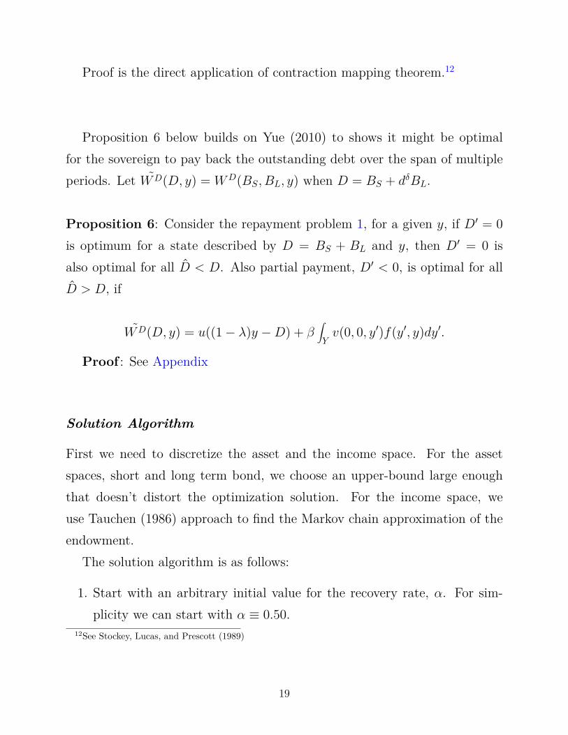
Proof is the direct application of contraction mapping theorem.12

Proposition 6 below builds on Yue (2010) to shows it might be optimalfor the sovereign to pay back the outstanding debt over the span of multipleperiods. Let WD(D, y) = WD(BS, BL, y) when D = BS + dδBL.

Proposition 6: Consider the repayment problem 1, for a given y, if D′ = 0is optimum for a state described by D = BS + BL and y, then D′ = 0 isalso optimal for all D < D. Also partial payment, D′ < 0, is optimal for allD > D, if

WD(D, y) = u((1− λ)y −D) + β∫Yv(0, 0, y′)f(y′, y)dy′.

Proof : See Appendix

Solution Algorithm

First we need to discretize the asset and the income space. For the assetspaces, short and long term bond, we choose an upper-bound large enoughthat doesn’t distort the optimization solution. For the income space, weuse Tauchen (1986) approach to find the Markov chain approximation of theendowment.

The solution algorithm is as follows:

1. Start with an arbitrary initial value for the recovery rate, α. For sim-plicity we can start with α ≡ 0.50.

12See Stockey, Lucas, and Prescott (1989)

19

2. Choose arbitrary values for bond prices, qS and qB. One can assign therisk-free prices as the initial values.

3. Solve the sovereign’s problem and derive the policy functions, repaymentand default sets.

4. Update the prices according to 4 and 5 . Find the difference betweenthe initial prices and the updated ones. Solve the sovereign’s problemin step 3 until the updated prices are the close enough to the the onescalculated before.

5. Find the recovery rate that solves the Nash bargaining game in 2. Findthe difference between the initial value and the updated one, and startover from step 3 as long as this difference is above the preset tolerance.

4 Quantitative Analysis

Parametrization

Table 1 shows the selected parameters for the quantitative analysis. As men-tioned before, preferences are modeled with a CARA utility function. Fol-lowing the literature, the coefficient of risk aversion, σ, is set to two:

u(C) = C1−σ

1− σ.

Endowment process is estimated using Argentina’s GDP using data fromMinistry of Finance (MECON). The quarterly data (real, seasonally adjusted)starts from the first quarter of 1980 till the default episode of 2001, the lastquarter of 2001. As in Arellano (2008), this paper assumes a log-normalAR(1) process for the GDP:

20

log(yt) = ρ log(yt−1) + εt, E[ε] = 0 and E[ε2] = η2

The estimated persistence, ρ and error standard deviation, η, are ρ = 0.95and η = 0.02. Then Markov chain with 21 discrete endowment state is con-structed Using Tauchen (1986).

The annual risk-free interest rate is set to r = 4%, which is the average1-year yield of the US bonds in that period. Decay rate, δ = 0.936 is se-lected to represent 10-year default-free duration. Output loss during defaultis λ = 2%, as suggested by Sturzenegger (2002).

Time preference, β, and borrower’s bargaining power, θ are calibrated tomatch the model moments to the observed data. Time preference is calibratedto match the default frequency in data. According to Reinhart, Rogoff, andSavastano (2003) Argentina experienced four default episodes from 1824 to1999. Including the 2001 default results in an annual (quarterly) default fre-quency equals to 2.8% (0.7%). According to Benjamin and Wright (2009),the average debt recovery rate in the 2001 default was 37%. In order to matchthis moment, the debtor’ bargaining power, θ is calibrated to θ = 0.83.

Simulation Results

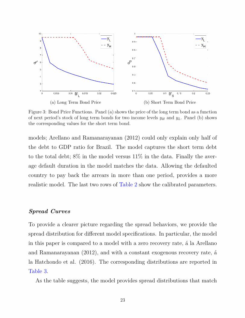
Figure 3 plots the price functions for short term and long term bonds asa function of choice of short term and long term debts, respectively. Toillustrate the role of endowment, the prices are depicted for high and low

21

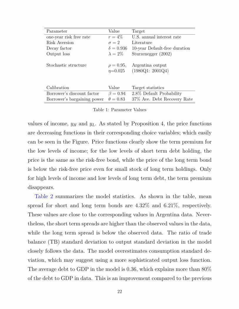
Parameter Value Targetone-year risk free rate r = 4% U.S. annual interest rateRisk Aversion σ = 2 LiteratureDecay factor δ = 0.936 10-year Default-free durationOutput loss λ = 2% Sturzenegger (2002)

Stochastic structure ρ = 0.95, Argentina outputη=0.025 (1980Q1: 2001Q4)

Calibration Value Target statisticsBorrower’s discount factor β = 0.94 2.8% Default ProbabilityBorrower’s bargaining power θ = 0.83 37% Ave. Debt Recovery Rate

Table 1: Parameter Values

values of income, yH and yL. As stated by Proposition 4, the price functionsare decreasing functions in their corresponding choice variables; which easilycan be seen in the Figure. Price functions clearly show the term premium forthe low levels of income; for the low levels of short term debt holding, theprice is the same as the risk-free bond, while the price of the long term bondis below the risk-free price even for small stock of long term holdings. Onlyfor high levels of income and low levels of long term debt, the term premiumdisappears.

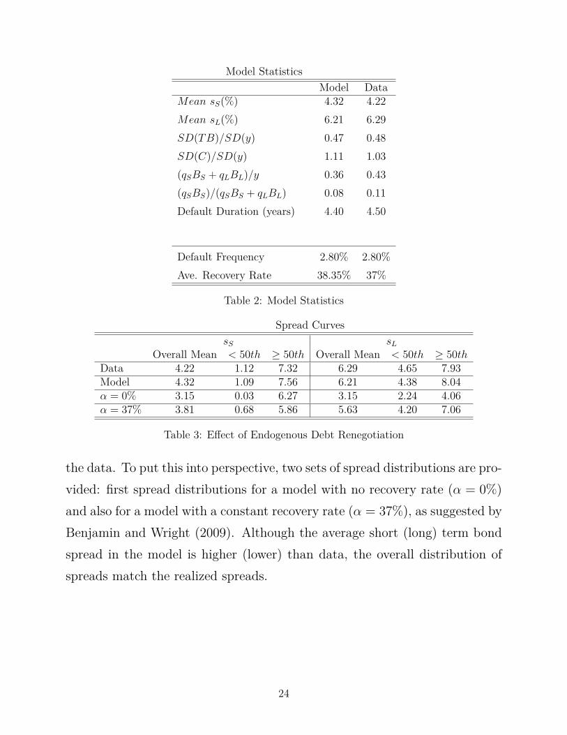
Table 2 summarizes the model statistics. As shown in the table, meanspread for short and long term bonds are 4.32% and 6.21%, respectively.These values are close to the corresponding values in Argentina data. Never-theless, the short term spreads are higher than the observed values in the data,while the long term spread is below the observed data. The ratio of tradebalance (TB) standard deviation to output standard deviation in the modelclosely follows the data. The model overestimates consumption standard de-viation, which may suggest using a more sophisticated output loss function.The average debt to GDP in the model is 0.36, which explains more than 80%of the debt to GDP in data. This is an improvement compared to the previous

22

(a) Long Term Bond Price (b) Short Term Bond Price

Figure 3: Bond Price Functions. Panel (a) shows the price of the long term bond as a functionof next period’s stock of long term bonds for two income levels yH and yL. Panel (b) showsthe corresponding values for the short term bond.

models; Arellano and Ramanarayanan (2012) could only explain only half ofthe debt to GDP ratio for Brazil. The model captures the short term debtto the total debt; 8% in the model versus 11% in the data. Finally the aver-age default duration in the model matches the data. Allowing the defaultedcountry to pay back the arrears in more than one period, provides a morerealistic model. The last two rows of Table 2 show the calibrated parameters.

Spread Curves

To provide a clearer picture regarding the spread behaviors, we provide thespread distribution for different model specifications. In particular, the modelin this paper is compared to a model with a zero recovery rate, a la Arellanoand Ramanarayanan (2012), and with a constant exogenous recovery rate, ala Hatchondo et al. (2016). The corresponding distributions are reported inTable 3.

As the table suggests, the model provides spread distributions that match

23

Model StatisticsModel Data

Mean sS(%) 4.32 4.22Mean sL(%) 6.21 6.29SD(TB)/SD(y) 0.47 0.48SD(C)/SD(y) 1.11 1.03(qSBS + qLBL)/y 0.36 0.43(qSBS)/(qSBS + qLBL) 0.08 0.11Default Duration (years) 4.40 4.50

Default Frequency 2.80% 2.80%Ave. Recovery Rate 38.35% 37%

Table 2: Model Statistics

Spread CurvessS sL

Overall Mean < 50th ≥ 50th Overall Mean < 50th ≥ 50thData 4.22 1.12 7.32 6.29 4.65 7.93Model 4.32 1.09 7.56 6.21 4.38 8.04α = 0% 3.15 0.03 6.27 3.15 2.24 4.06α = 37% 3.81 0.68 5.86 5.63 4.20 7.06

Table 3: Effect of Endogenous Debt Renegotiation

the data. To put this into perspective, two sets of spread distributions are pro-vided: first spread distributions for a model with no recovery rate (α = 0%)and also for a model with a constant recovery rate (α = 37%), as suggested byBenjamin and Wright (2009). Although the average short (long) term bondspread in the model is higher (lower) than data, the overall distribution ofspreads match the realized spreads.

24

Discussion

In this section, an intuitive argument is presented to explain the behavior ofthe interest rate spreads in the models with and without debt renegotiation.First notice the model with endogenous renegotiation results in larger spreadmeans. In addition, according to Table 2, our model delivers higher debt toGDP ratio. The association between these two can be explained by recallingthat the high spreads occur at the high levels of debt. In other words, since inour model the default is optimal at higher levels of debt, the observed spreads(spreads before the default episodes) are larger than the models without debtrenegotiation.

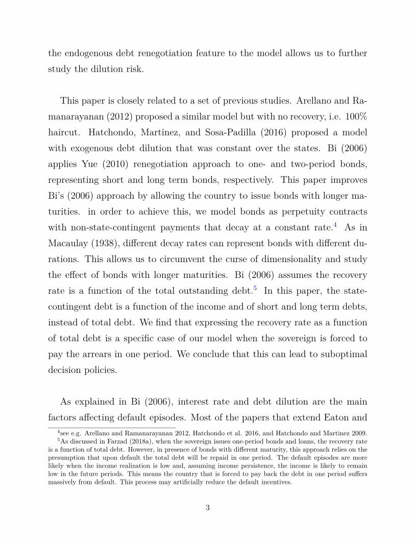
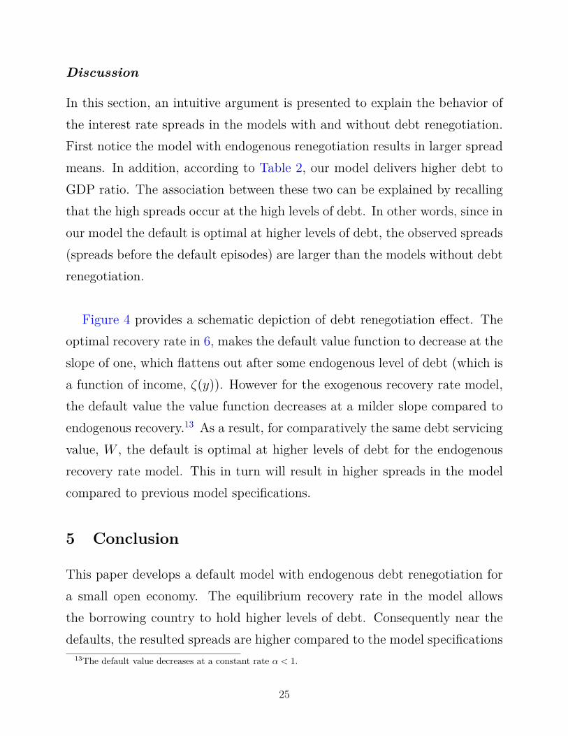
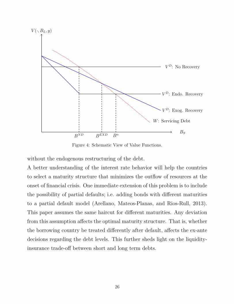
Figure 4 provides a schematic depiction of debt renegotiation effect. Theoptimal recovery rate in 6, makes the default value function to decrease at theslope of one, which flattens out after some endogenous level of debt (which isa function of income, ζ(y)). However for the exogenous recovery rate model,the default value the value function decreases at a milder slope compared toendogenous recovery.13 As a result, for comparatively the same debt servicingvalue, W , the default is optimal at higher levels of debt for the endogenousrecovery rate model. This in turn will result in higher spreads in the modelcompared to previous model specifications.

5 Conclusion

This paper develops a default model with endogenous debt renegotiation fora small open economy. The equilibrium recovery rate in the model allowsthe borrowing country to hold higher levels of debt. Consequently near thedefaults, the resulted spreads are higher compared to the model specifications

13The default value decreases at a constant rate α < 1.

25

BND BEXD Bα

V (·, BL, y)

V D: No Recovery

V D: Endo. Recovery

V D: Exog. Recovery

W : Servicing Debt

BS

Figure 4: Schematic View of Value Functions.

without the endogenous restructuring of the debt.A better understanding of the interest rate behavior will help the countriesto select a maturity structure that minimizes the outflow of resources at theonset of financial crisis. One immediate extension of this problem is to includethe possibility of partial defaults; i.e. adding bonds with different maturitiesto a partial default model (Arellano, Mateos-Planas, and Rios-Rull, 2013).This paper assumes the same haircut for different maturities. Any deviationfrom this assumption affects the optimal maturity structure. That is, whetherthe borrowing country be treated differently after default, affects the ex-antedecisions regarding the debt levels. This further sheds light on the liquidity-insurance trade-off between short and long term debts.

26

Appendix

Proof of Proposition 1: The proof follows Yue (2010). We can show in thesimilar manner that following problems have a fixed point:

1. The bond price functions, given the default and repayment sets, thepolicy functions of the borrowing country, and the recovery rate,

2. The debt renegotiation problem, given the bond prices,

3. The borrowing country value functions, given the bond prices and re-cover rate.

Proof of Lemma 1:

WD(BS, BL, y) = max0≤B′S≤BS , 0≤B′L≤BL, 0≤C

u(C)+β∫YWD(B′S, B′L, y′)f(y′|y)dy′

C +BS +BL = (1− λ)y + B′S1 + r

+ B′L − δBL

1 + r − δ

C = (1− λ)y +[ B′S1 + r

−BS

]+[ B′L1 + r − δ

− BL(1 + r)1 + r − δ

]

Letting X = BL(1+r)1+r−δ , we can rewrite the above budget constraint as:

C = y +[ B′S1 + r

−BS

]+[ X ′L1 + r

−XL

]

C +BS +XL = (1− λ)y +[ B′S1 + r

+ X ′L1 + r

]

Since X ′L ≤ XL implies B′L ≤ BL, 1 is invariant to any transfer of debt as

27

long as BS + BL(1+r)1+r−δ is fixed. Since V D solely depends on WD, debtor’s sur-

plus is invariant to a transformation shown above. The present values showcreditors’ surplus is invariant to such transformations as well.

Proof of Proposition 214:Appealing to Lemma 1, WD and consequently V D is a function of α(BS +

dδBL). Hence ∆D = V D − V Aut is a function of α(BS + dδBL). ∆C in 2 isalso a function α(BS + dδBL). This means the solution to 2 can be writtenas α(BS + dδBL) = ζ(y). Since α ∈ [0, 1], α = 1, ∀(BS + dδBL) ≤ ζ(y) and

ζ(y)(BS+dδBL) , ∀(BS + dδBL) ≥ ζ(y).

Proof of Proposition 3:The proof follows Eaton and Gersovitz (1981) and Chatterjee et al. (2007),

Arellano(2008), and Yue(2010). Since the value of default is independent oftotal dated debt level, for any debt level above D1 =≤ D2, W (B2

S, B2L, y) ≤

W (B1S, B

1L, y) ≤ V D(B1, L1, y) = V D(B2, L2, y). Proof of the corollaries is by

contradiction.

Proof of Proposition 4:

First notice by increasing short term bonds R(B′S, B′L) and D(B′S, B′L) in3 will (weakly) shrink and expand, respectively. Also α (weakly) decreasesaccording to proposition 2. Hence, the price of short term bond is (weakly)decreasing.

14Extension of Yue (2010).

28

For the long term bonds, we can appeal to the contraction mapping charac-teristics.15 Using the fact that by increasing long term bonds R(B′S, B′L) andD(B′S, B′L) in 3 will (weakly) shrink and expand, respectively, one can showthat the price of long term bond is a decreasing function in BL.

Proof of Proposition 6:The proposition is a direct consequence of properties of policy functions;

if D1 > D2, then D′1 > D′2.Notice WD(D, y) is decreasing and concave inD; ifD1 > D2, then WD(D1, y) <

WD(D2, y) and ∂∂DW

D(D1, y′) < ∂

∂DWD(D2, y

′) < 0.

By contradiction, let D′1 < D′2 for D1 > D2. The optimization problemrequires:

11 + r

u′(y + D′11 + r

−D1) = −β∫Y

∂

∂DWD(D′1, y′)f(y′, y)dy′

11 + r

u′(y + D′21 + r

−D2) = −β∫Y

∂

∂DWD(D′2, y′)f(y′, y)dy′

However due to concavity of u,

u′(y + D′11 + r

−D1) ≥ u′(y + D′21 + r

−D2)

Which means,

−β∫Y

[ ∂∂D

WD(D′1, y′)−∂

∂DWD(D′2, y′)

]f(y′, y)dy′ ≥ 0

Which is a contraction.

15See Stokey, Lucas, and Prescott (1989)

29

References

[1] Aguiar, M. and Gopinath, G. (2006), “Defaultable debt, interest ratesand the current account.”, Journal of International Economics, 69 (1):64–83.

[2] Arellano, C. (2008) “Default Risk and Income Fluctuations in EmergingEconomies.” American Economic Review, 98 (3): 690–712.

[3] Arellano, C., and Ramanarayanan, A. (2012). “Default and the MaturityStructure in Sovereign Bonds.” Journal of Political Economy, 120(2), 187-232.

[4] Arellano C., X. Mateos-Planas, and J. Rios-Rull, (2013), “Partial De-fault”, Manuscript.

[5] Bai, Y. and J. Zhang (2012), “Duration of Sovereign Debt Renegotia-tion”, Journal of International Economics, 86(2): 252-268.

[6] Benjamin, D. and M. L. Wright (2009), “Recovery Before Redemption:A Theory of Delays in Sovereign Debt Renegotiations”,

[7] Bi, R. 2006. “Debt Dilution and the Maturity Structure of SovereignBonds.” Manuscript, University of Maryland.

[8] Broner, F. A., Lorenzoni, G. and Schmukler, S. L. (2013), “Why DoEmerging Economies Borrow Short Term?” Journal of the European Eco-nomic Association, 11: 67-100.

[9] Bulow, J., Rogoff, K., (1989a). “A Constant Recontracting Model ofSovereign Debt.”, Journal of Political Economy. 97: 155–178.

[10] Chatterjee, S., and B. Eyigungor. (2012). “Maturity, Indebtedness, andDefault Risk.” American Economic Review, 102 (6): 2674–99.

30

[11] Eaton, J., and M. Gersovitz. (1981), “Debt with Potential Repudia-tion: Theoretical and Empirical Analysis.” Revie of Economic Studies48: 289–309.

[12] D’Erasmo P. (2008), “Government Reputation and Debt Repayment inEmerging Economies”, Manuscript, University of Texas, Austin.

[13] Das U. S., M. G. Papaioannou, and C. Trebesch, (2012), “RestructuringSovereign Debt: Lessons from Recent History”, IMF Manuscript.

[14] Farzad T. (2018a), “Debt Instruments and Sovereign Defaults.”, Univer-sity of California, Riverside, Manuscript.

[15] Farzad T. (2018c),“Partial Defaults and Debt Renegotiation”, Universityof California, Riverside, Manuscript.

[16] Hatchondo, J. C., and L. Martinez. 2009.“Long-Duration Bonds andSovereign Defaults.” Journal of International Economics, 79: 117–25.

[17] Hatchondo, J. C., L. Martinez, and C. Sosa-Padilla, (2016), “Debt Dilu-tion and Sovereign Default Risk.”, Journal of Political Economy, 124(5):1383 - 1422.

[18] Macaulay, F. R., (1938), “Bond Yields, Economic ’Drift’, and the Pricesof Common Stocks”, p. 128-162 in , Some Theoretical Problems Sug-gested by the Movements of Interest Rates, Bond Yields and Stock Pricesin the United States since 1856, National Bureau of Economic Research,Inc.

[19] Neumeyer, P. and F. Perri (2005), ““Business Cycles in Emerging Economies:The Role of Interest Rates.”, Journal of Monetary Economics, 52: 345-80.

[20] Reinhart, C., K. Rogoff, and M. A. Savastano, (2003), “Debt Intoler-ance”, Brookings Papers on Economic Activity, 34(1): 1-74.

31

[21] Stokey, N. L., E. C. Prescott, and R. E. Lucas, Robert E. (1989). “Re-cursive methods in economic dynamics.” Cambridge, Mass : HarvardUniversity Press.

[22] Sturzenegger, F. and J. Zettelmeyer, (2008), “Haircuts: Estimating in-vestor losses in sovereign debt restructurings, 1998-2005”, Journal of In-ternational Money and Finance, 27(5): 780-805.

[23] Tauchen, G. (1986), “Finite State Markov-Chain Approximations to Uni-variate and Vector Autoregressions.” Economics Letters, 20 (2): 177–81.

[24] Yue V. Z. (2010), “Sovereign default and debt renegotiation.”, Journalof international Economics, 80(2): 176-187.

32