Matthias Kawski. “ Visualizing Agrachëv’s curvature” Banach Institute, Bedlevo June, 2003 kawski [email protected] Visualizing Agrachëv’s

http://math.asu.edu/~kawski [email protected]

Matthias Kawski. “ Visualizing Agrachëv’s curvature” Banach Institute, Bedlevo June, 2003

Visualizing Agrachëv’s curvature of optimal control

Matthias Kawski

and Eric Gehrig

Arizona State University

Tempe, U.S.A.

This work was partially supported by NSF grant DMS 00-72369.



Outline• Motivation of this work• Brief review of some of Agrachëv’s theory, and

of last year’s work by Ulysse Serres• Some comments on ComputerAlgebraSystems

“ideally suited” “practically impossible”• Current efforts to “see” curvature of optimal cntrl.

– how to read our pictures– what one may be able to see in our pictures

• Conclusion: A useful approach? Promising 4 what?



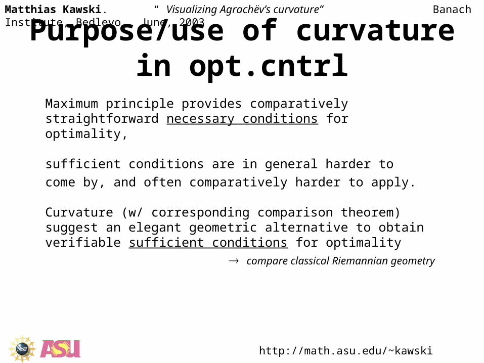
Purpose/use of curvature in opt.cntrl

Maximum principle provides comparatively straightforward necessary conditions for optimality,

sufficient conditions are in general harder to

come by, and often comparatively harder to apply.

Curvature (w/ corresponding comparison theorem)suggest an elegant geometric alternative to obtain verifiable sufficient conditions for optimality

compare classical Riemannian geometry



Curvature of optimal control

•understand the geometry•develop intuition in basic examples•apply to obtain new optimality results



Classical geometry: Focusing geodesics

Positive curvature focuses geodesics, negative curvature “spreads them out”.

Thm.: curvature negative geodesics (extremals) are optimal (minimizers)

The imbedded surfaces view, and the color-coded intrinsic curvature view



Definition versus formula

A most simple geometric definition

- beautiful and elegant.

but the formula in coordinates is incomprehensible

(compare classical curvature…)

(formula from Ulysse Serres, 2001)





Aside: other interests / plans

• What is theoretically /practically feasible to compute w/ reasonable resources? (e.g. CAS: “simplify”, old: “controllability is NP-hard”, MK 1991)

• Interactive visualization in only your browser…– “CAS-light” inside JAVA

(e.g. set up geodesic eqns)– “real-time” computation of

geodesic spheres(e.g. “drag” initial point w/

mouse, or continuously vary

parameters…)

“bait”, “hook”, like Mandelbrot fractals….

Riemannian, circular parabloid



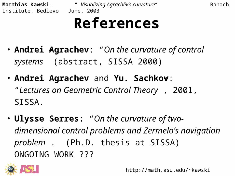
References

• Andrei Agrachev: “On the curvature of control systems”

(abstract, SISSA 2000)

• Andrei Agrachev and Yu. Sachkov:

“Lectures on Geometric Control Theory”, 2001, SISSA.

• Ulysse Serres: “On the curvature of two-dimensional

control problems and Zermelo’s navigation problem”.

(Ph.D. thesis at SISSA) ONGOING WORK ???



From: Agrachev / Sachkov: “Lectures on Geometric Control Theory”, 2001






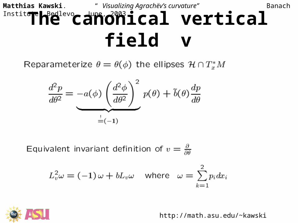
Next: Define distinguished parameterization of H x




The canonical vertical field v






Jacobi equation in moving frameFrame

or:



Zermelo’s navigation problem

“Zermelo’s navigation formula”



formula for curvature ?

total of 782 (279) terms in num, 23 (7) in denom. MAPLE can’t factor…



Use U. Serre’s form of formula

so far have still been unable to coax MAPLE into obtaining

this without doing all “simplification” steps manually

polynomial in f and first 2 derivatives, trig polynomial in , interplay of 4 harmonics



First pictures: fields of polar plots

• On the left: the drift-vector field (“wind”)

• On the right: field of polar plots of (x1,x2,)

in Zermelo’s problem u* = . (polar coord on fibre)

polar plots normalized and color enhanced: unit circle zero curvature

negative curvature inside greenish positive curvature outside pinkish



Example: F(x,y) = [sech(x),0]

NOT globally scaled. colors for + and - scaled independently.



Example: F(x,y) = [0, sech(x)]


Question: What do optimal paths look like? Conjugate points?



Example: F(x,y) = [ - tanh(x), 0]




From now on: color code only(i.e., omit radial plots)



Special case: linear drift

• linear drift F(x)=Ax, i.e., (dx/dt)=Ax+eiu

• Curvature is independent of the base point x, study dependence on parameters of the drift

(x1,x2,) = ()

This case is being studied in detail by U.Serres.Here we only give a small taste of the richness

of even this very special simple class of systems



Linear drift, preparation I

• (as expected), curvature commutes with rotations

quick CAS check: , ,B

( )cos ( )sin

( )sin ( )cos

a b

c d

( )cos ( )sin

( )sin ( )cos

kB19 a d

16

3

8d

2( )cos 2 2 3

4b

2( )cos 2 2 3

4c2

( )cos 2 2 3

8a

2( )cos 2 2 3

32c

2( )cos 4 4 :=

3

32b

2( )cos 4 4 3

8c a ( )sin 2 2 21 c b

16

9

8b a ( )sin 2 2 9

8c d ( )sin 2 2 23 a

2

32

21 b2

32

23 d2

32

3

32d

2( )cos 4 4 3

32a

2( )cos 4 4 3

16c a ( )sin 4 4 3

16c d ( )sin 4 4 3

16b a ( )sin 4 4

3

16a d ( )cos 4 4 3

16c b ( )cos 4 4 3

16d b ( )sin 4 4 3

8d b ( )sin 2 2 21 c

2

32

> k['B']:=combine(simplify(zerm(Bxy,x,y,theta),trig));



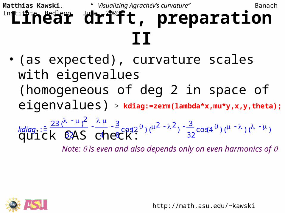
Linear drift, preparation II

• (as expected), curvature scales with eigenvalues(homogeneous of deg 2 in space of eigenvalues)

quick CAS check:

:= kdiag 23 ( ) 2

32

4

3

8( )cos 2 ( )2 2 3

32( )cos 4 ( ) ( )

> kdiag:=zerm(lambda*x,mu*y,x,y,theta);

Note: is even and also depends only on even harmonics of



Linear drift

• if drift linear and ortho-gonally diagonalizable then no conjugate pts(see U. Serres’ for proof, here suggestive picture only)

> kdiag:=zerm(x,lambda*y,x,y,theta);

:= kdiag 23 ( )1 2

32

4

3

8( )cos 2 ( ) 1 2 3

32( )cos 4 ( ) 1 ( )1



Linear drift

• if linear drift has non-trivial Jordan block then a little bit ofpositive curvature exists

• Q: enough pos curv forexistence of conjugate pts?

> kjord:=zerm(lambda*x+y,lambda*y,x,y,theta);

:= kjord 21

32

2

4

3

4( )cos 2 3

4( )sin 2 3

32( )cos 4



Some linear drifts

jordan w/ =13/12

diag w/ =10,-1

diag w/ =1+i,1-i

Question: Which case is good for optimal control?



Ex: A=[1 1; 0 1]. very little pos curv



Scalings: + / - , local / globalsame scale for pos.& neg. parts

pos.& neg. parts color-scaled independently

local

color-scales,

each fibre

independ.

global

color-scale,

same for

every fibre

here: F(x) = ( 0, sech(3*x1))



Example:F(x)=[0,sech(3x)]

scaled locally / globally



F(x)=[0,sech(3x)]

globally scaled. colors for + and - scaled simultaneously.



F(x)=[0,sech(3x)]

globally scaled. colors for + and - scaled simultaneously.



Conclusion

• Curvature of control: beautiful subjectpromising to yield new sufficiency results

• Even most simple classes of systems far from understood• CAS and interactive visualization promise to be useful

tools to scan entire classes of systems for interesting, “proof-worthy” properties.

• Some CAS open problems (“simplify”). Numerically fast implementation for JAVA????

• Zermelo’s problem particularly nice because everyone has intuitive understanding, wants to argue which way is best, then see and compare to the true optimal trajectories.



Documents

Matthias Kawski. “ Visualizing Agrachëv’s curvature” Banach Institute, Bedlevo June, 2003 kawski [email protected] Visualizing Agrachëv’s