Accepted for publication in IcarusPreprint typeset using LATEX style AASTeX6 v. 1.0

THE EARLY INSTABILITY SCENARIO: MARS’ MASS EXPLAINED BY JUPITER’S ORBIT

Matthew S. Clement1, Nathan A. Kaib2, Sean N. Raymond3 & John E. Chambers1

1Earth and Planets Laboratory, Carnegie Institution for Science, 5241 Broad Branch Road, NW, Washington, DC 20015, USA2HL Dodge Department of Physics Astronomy, University of Oklahoma, Norman, OK 73019, USA3Laboratoire d’Astrophysique de Bordeaux, Univ. Bordeaux, CNRS, B18N, alle Geoffroy Saint-Hilaire, 33615 Pessac, France

ABSTRACT

The formation of the solar system’s giant planets predated the ultimate epoch of massive impacts that

concluded the process of terrestrial planet formation. Following their formation, the giant planets’

orbits evolved through an episode of dynamical instability. Several qualities of the solar system have

recently been interpreted as evidence of this event transpiring within the first ∼100 Myr after the

Sun’s birth; around the same time as the final assembly of the inner planets. In a series of recent

papers we argued that such an early instability could resolve several problems revealed in classic

numerical studies of terrestrial planet formation; namely the small masses of Mars and the asteroid

belt. In this paper, we revisit the early instability scenario with a large suite of simulations specifically

designed to understand the degree to which Earth and Mars’ formation are sensitive to the specific

evolution of Jupiter and Saturn’s orbits. By deriving our initial terrestrial disks directly from recent

high-resolution simulations of planetesimal accretion, our results largely confirm our previous findings

regarding the instability’s efficiency of truncating the terrestrial disk outside of the Earth-forming

region in simulations that best replicate the outer solar system. Moreover, our work validates the

primordial 2:1 Jupiter-Saturn resonance within the early instability framework as a viable evolutionary

path for the solar system. While our simulations elucidate the fragility of the terrestrial system during

the epoch of giant planet migration, many realizations yield outstanding solar system analogs when

scrutinized against a number of observational constraints. Finally, we highlight the inability of models

to form adequate Mercury-analogs and the low eccentricities of Earth and Venus as the most significant

outstanding problems for future numerical studies to resolve.

1. INTRODUCTION

Giant gaseous planets form precipitously within proto-

planetary disks that dissipate on timescales of just a

few Myr (Mizuno 1980; Haisch et al. 2001; Mamajek &

Hillenbrand 2008; Pascucci et al. 2009). In the stan-

dard paradigm, conditions in the solar nebula were ap-

propriate to produce a sequential system of appropri-

ately massed giant planet cores directly via pebble ac-

cretion (e.g.: Morbidelli & Nesvorny 2012; Lambrechts

& Johansen 2012; Chambers 2014; Levison et al. 2015a)

or gravitational collapse (e.g.: Boss 1997; Mayer et al.

2002). In addition to feeding the outer planets’ massive

envelopes, the nebular gas conspired to force the giant

planets into a tight chain of mutually resonant orbits

via powerful gravitational torques (e.g.: Masset & Snell-

grove 2001; Morbidelli & Crida 2007; Pierens & Nelson

2008; Zhang & Zhou 2010; D’Angelo & Marzari 2012).

The Nice Model (Tsiganis et al. 2005; Gomes et al. 2005;

Morbidelli et al. 2005; Nesvorny & Morbidelli 2012) ar-

gues that a number of observed dynamical structures in

the solar system (e.g.: Levison et al. 2008; Morbidelli

et al. 2009b; Nesvorny et al. 2013; Nesvorny 2015a,b;

Roig & Nesvorny 2015) are best explained by the disso-

lution of this resonant chain through an epoch of dy-

namical instability. Among other qualities, the exis-

tence of irregular satellites around all four giant planets

(Nesvorny et al. 2014a,b) strongly favors an epoch of

planetary encounters having occurred sometime in the

solar system’s past.

While a full review of the Nice Model is beyond the

scope of this manuscript (see, for example: Nesvorny

2018; Clement et al. 2018, 2021b), it is important to

understand that the current consensus version invokes

the existence of either one or two additional ice giants

(Nesvorny 2011, note that we only consider cases with

five primordial giant planets in this work). The ejection

of these planets in successful numerical simulations of

the highly-stochastic instability serves to both maximize

the probability of retaining four outer planets (Nesvorny

& Morbidelli 2012), and minimize the time powerful

resonances with Jupiter and Saturn inhabit certain re-

gions of the inner solar system (e.g.: Brasser et al. 2009;

arX

iv:2

106.

0527

6v1

[as

tro-

ph.E

P] 9

Jun

202

1

2

Minton & Malhotra 2010; Walsh & Morbidelli 2011;

Roig & Nesvorny 2015; Roig et al. 2016).

Early investigations of the Nice Model advocated for

a very specific timing of the event (Gomes et al. 2005;

Levison et al. 2011; Deienno et al. 2017): ∼3.9 billion

years ago in order to provide a natural trigger for the late

heavy bombardment (a spike in cratering rates in the in-

ner solar system inferred via basin ages determined from

the Apollo samples: Tera et al. 1974). However, mod-

ern isotopic dating techniques (e.g.: Norman et al. 2006;

Grange et al. 2013; Merle et al. 2014; Mercer et al. 2015;

Boehnke & Harrison 2016) and new high-resolution im-

agery of the Moon’s surface seem to imply a smooth

decline in cratering rather than a terminal onslaught of

impacts (Zellner 2017). In response to these revelations,

dynamical investigations have increasingly sought to un-

derstand how varying the instability’s precise timing af-

fects the ability of models to match important observa-

tional and geochemical constraints. Several recent stud-

ies in this mold have convincingly argued that particu-

lar aspects of the solar systems favor an early (t . 100

Myr) instability. These include the survival of Jupiter’s

Patroclus-Menoetius binary trojan pair (Nesvorny et al.

2018), the dichotomous inventories of highly siderophile

elements incorporated in the mantles of the Earth and

Moon following the formation of their cores (Morbidelli

et al. 2018; Brasser et al. 2020), resetting ages of various

inner solar system meteorites (Mojzsis et al. 2019), col-

lisional families in the asteroid belt with inferred ages

&4.0 Gyr (Delbo’ et al. 2017; Delbo et al. 2019), and the

fact that late instabilities are highly improbable from a

dynamical standpoint (Quarles & Kaib 2019; Ribeiro

et al. 2020). Thus, a diffuse consensus has developed

over the past several years in support of the instability’s

occurrence within the first ∼100 Myr after nebular gas

dispersal.

An early instability implies that the event occurred

around the same time as the Moon-forming impact (t '30-100 Myr, e.g.: Touboul et al. 2007), and by exten-

sion coincident with the late stages of terrestrial planet

formation (Wood & Halliday 2005; Kleine et al. 2009;

Rudge et al. 2010; Kleine & Walker 2017). This is po-

tentially advantageous as the delicate orbits of the fully

formed terrestrial planets (namely those of Mercury and

Mars) are easily destabilized by the Nice Model insta-

bility (Brasser et al. 2009; Agnor & Lin 2012; Brasser

et al. 2013; Kaib & Chambers 2016). In the classical

model of terrestrial planet formation (Wetherill 1980,

1991; Chambers & Wetherill 1998) the inner planets

collisionally accrete from an ocean of ∼0.01-0.1 M⊕ em-

bryos (Kokubo & Ida 1996, 1998, 2000; Chambers 2006)

and smaller, D ' 10-1000 km planetesimals (Johansen

et al. 2007; Morbidelli et al. 2009a; Delbo’ et al. 2017).

If the terrestrial forming disk extends to the asteroid

belt’s outer edge (consistent with the minimum mass so-

lar nebula: Weidenschilling 1977; Hayashi 1981), the re-

sulting model-generated Mars analogs consistently pos-

sess masses similar to those of Earth and Venus (an or-

der of magnitude more massive than the real planet:

Chambers 2001; Raymond et al. 2009). Similarly, mas-

sive planets in the asteroid belt are common outcomes

in classic studies of terrestrial planet formation (Cham-

bers & Wetherill 2001). A straight-forward resolution to

these problems involves restricting the amount of ma-

terial available for Mars’ accretion by either truncat-

ing the disk’s outer edge (Wetherill 1978; Agnor et al.

1999; Morishima et al. 2008; Hansen 2009) or altering its

structure (Chambers & Cassen 2002; Izidoro et al. 2014,

2015). These initial conditions might be explained by

either radial variances in the efficiency of planetesimal

formation (Levison et al. 2015b; Drazkowska et al. 2016;

Raymond & Izidoro 2017), or the two-phased inward-

outward migration of Jupiter and Saturn during the gas-

disk phase (e.g.: the Grand Tack model: Walsh et al.

2011; Pierens & Raymond 2011; Jacobson & Morbidelli

2014; Brasser et al. 2016). For recent reviews of these

models see: Morbidelli et al. (2012), Izidoro & Raymond

(2018) and Raymond et al. (2018).

An alternative solution to the small Mars problem

relies on the influence of Jupiter and Saturn’s eccen-

tric forcing (Raymond et al. 2009; Lykawka & Ito 2013;

Bromley & Kenyon 2017). Clement et al. (2018) stud-

ied the effects of an unusually early Nice Model (t . 10

Myr) on the forming terrestrial planets and found rea-

sonable solar system analogs result regularly in models

where the instability excites the eccentricities of Jupiter

and Saturn before Mars’ mass exceeds its modern value.

By stunting Mars’ growth in this manner, the instability

essentially sets the planet’s geological growth timescale;

thus providing a natural explanation for the Mars’ rapid

inferred accretion time (Nimmo & Agnor 2006; Dauphas

& Pourmand 2011; Kruijer et al. 2017). Subsequent in-

vestigations by Deienno et al. (2018) and Clement et al.

(2019c) leveraging high-resolution simulations of the as-

teroid belt found the early instability scenario to be

broadly consistent with the belt’s low-mass and dynam-

ically excited state. In particular, adequately exciting

and depleting a primordially massive belt (e.g.: Petit

et al. 2001) necessitates an instability strong enough

to significantly perturb or destroy the system of fully

formed terrestrial planets (Agnor & Lin 2012; Kaib &

Chambers 2016); thus axiomatically requiring an early

Nice Model. However, as a consequence of this vio-

lent dynamical event the final Earth and Venus analogs

formed in early instability simulations (Clement et al.

2018; Nesvorny et al. 2021) typically possess eccentric-

ities and inclinations that are too large. Clement et al.

(2019b) found marginally improved outcomes by con-

3

sidering the tendency of collisional fragments and de-

bris to damp the forming planets’ orbits (Chambers

2013; Walsh & Levison 2016), however the efficiency of

this process is highly dependent on the numerical im-

plementation (for an opposing view see: Deienno et al.

2019). Nevertheless, reconciling the dynamically cold

orbits and, to a lesser degree, the compact radial sepa-

ration of Earth and Venus remains a major shortcoming

of terrestrial planet formation models in general (Ray-

mond et al. 2018).

In this manuscript we return to the early instability

framework of Clement et al. (2018) and Clement et al.

(2019b), henceforth Paper I and Paper II, respectively,

with new simulations incorporating a number of impor-

tant modifications. In particular, several new develop-

ments in our understanding of the solar system’s early

evolution implore us to reexamine the early instability

scenario:

1. The instability itself is inherently stochastic, and

only a few percent of numerical realizations yield

giant planet configurations broadly akin to the

real outer solar system (Batygin & Brown 2010;

Nesvorny & Morbidelli 2012; Batygin et al. 2012;

Deienno et al. 2017). Thus, only a small number

of the original simulations in Paper I and Paper II

produced reasonable outer solar system analogs.

Indeed, many of the less successful terrestrial re-

sults were derived from simulations that under-

excited the eccentricities of Jupiter and Saturn (a

facet of the outer solar system that is challenging

to replicate with N-body simulations: Nesvorny

& Morbidelli 2012; Clement et al. 2021b, see be-

low). In this paper, we develop a new pipeline

that substantially increases our sample of appro-

priate giant planet evolutions with the aim of more

concretely understanding the dependence of the

early instability scenario’s viability on the eccen-

tricity excitation of the gas giants. Nesvorny et al.

(2021) considered a similar question by modeling

successful instabilities via cubic interpolation of

simulation outputs and concluded that the abil-

ity of the scenario to replicate Mars’ mass is not

related to the particular evolution of Jupiter and

Saturn. However, the authors did not control for

the instability’s timing, thus making it difficult to

disentangle the underlying cause of variations in

statistical outcomes between different batches of

simulations (discussed further in 3.2).

2. The investigations in Paper I, Paper II and

Nesvorny et al. (2021) exclusively considered Nice

Model scenarios where Jupiter and Saturn orig-

inate in a 3:2 MMR (mean motion resonance)

on circular orbits (e.g.: Morbidelli & Crida 2007;

Pierens & Nelson 2008). While such initial condi-

tions have demonstrated consistent success when

scrutinized against certain small body constraints

(see Nesvorny 2018, for a relevant review), it

is systematically challenging to adequately excite

Jupiter’s eccentricity (eJ) without over-exciting

Saturn’s eccentricity (eS) and driving its semi-

major axis (aS) into the distant solar system

(Clement et al. 2021b). This shortcoming is un-

fortunate given the apparent correlation between

the gas giants’ eccentricities and Mars’ mass (Ray-

mond et al. 2009; Clement et al. 2018). Pierens

et al. (2014) found that Jupiter and Saturn’s cap-

ture in the 2:1 MMR is possible given a specific

combinations of assumed disk parameters. Of par-

ticular relevance to the topic of terrestrial planet

formation and the small Mars problem, the gas gi-

ants carve out larger gaps in the nebular gas when

locked in the 2:1 resonance; thus allowing them to

attain inflated eccentricities prior to the instabil-

ity. Clement et al. (2021b) studied the outcomes

of these 2:1, high-eccentricity instabilities statisti-

cally and noted markedly improved success rates

compared to the primordial 3:2 MMR in terms

of matching Jupiter’s eccentricity without driv-

ing Saturn’s semi-major axis into the distant solar

system. As the giant planets’ resonant perturba-

tions in the terrestrial region occur over a more

restricted radial range in these new evolutions, it

is important to thoroughly study the implications

of the primordial 2:1 Jupiter-Saturn resonance on

the early instability scenario.

3. The initial conditions for the giant impact phase

supposed throughout the literature (as well as in

Papers I and II) are loosely based on the outcomes

of semi-analytic investigations of runaway growth

(e.g.: Kokubo & Ida 1996, 1998, 2000; Chambers

2006). However, the computational challenge of

directly resolving proto-planet growth from ∼100

km planetesimals makes it difficult to infer the

precise embryo and planetesimal distributions in

the terrestrial disk around the time of nebular

gas dissipation. Consequently, terrestrial planet

formation studies tend to either distribute equal-

mass embryos throughout the terrestrial disk (e.g.:

Chambers 2001; O’Brien et al. 2006), or assign

embryos masses that are proportional to the an-

alytic isolation mass (e.g.: Raymond et al. 2004,

2006, 2009). Advances in computing power have

recently made high-resolution N-body models of

runaway growth throughout the terrestrial disk

feasible (e.g.: Morishima et al. 2010; Carter et al.

2015; Walsh & Levison 2019; Wallace & Quinn

4

2019; Clement et al. 2020a; Woo et al. 2021). This

presents a novel opportunity to test the viability

of the early instability scenario with embryo and

planetesimal distributions derived from scratch.

Here, we utilize outputs from Walsh & Levison

(2019) and Clement et al. (2020a) around the time

of nebular dispersal when constructing our terres-

trial disks.

It is worth mentioning that contemporary terrestrial

planet formation models are incapable of consistently

generating Mercury analogs of the appropriate mass

(Chambers 2001; O’Brien et al. 2006; Lykawka & Ito

2017, 2019), composition (Hauck et al. 2013; Nittler

et al. 2017; Jackson et al. 2018), and radial offset from

Venus (Clement et al. 2019a). While we do not ne-

glect Mercury in the analysis sections of this paper

(we present a particularly interesting Mercury analog

in section 3.4), we also do not explicitly modify our

simulations to boost the likelihood of forming Mer-

cury (Lykawka & Ito 2017, 2019; Clement et al. 2021a;

Clement & Chambers 2021). Thus, the primary goals

of this paper are to validate the viability of the primor-

dial 2:1 Jupiter-Saturn resonance (Pierens et al. 2014;

Clement et al. 2021b) and the disk-evolved embryo and

planetesimal distributions from Walsh & Levison (2019)

and Clement et al. (2020a) within the early instability

framework of Paper I.

2. METHODS

2.1. Numerical Simulations

Our numerical approach largely follows the method-

ology established in Paper I. To ensure the instability

triggers at a predetermined time (i.e.: in conjunction

with a specific evolutionary state of the terrestrial disk)

we integrate our terrestrial disks (section 2.4) and gi-

ant planet configurations (section 2.3) separately before

combining both sets of bodies into a single simulation.

We construct these terrestrial disk inputs directly us-

ing time-outputs of interest from high-resolution simu-

lations of planetesimal accretion and runaway growth in

Walsh & Levison (2019) and Clement et al. (2020a). To

minimize interpolations, embryo populations are derived

exactly from all objects with M > 0.01 M⊕ (around the

mass of the Moon). Planetesimal distributions are in-

ferred by sampling from the remaining particles’ orbital

distributions.

We generate systems of resonant giant planets

(Nesvorny & Morbidelli 2012; Clement et al. 2021b, de-

scribed further in section 2.3) with fictitious forces de-

signed to mimic gas disk interaction (e.g.: Lee & Peale

2002). We then integrate the resultant resonant chains

in the presence of an external disk of primordial Kuiper

Belt Objects (KBOs, e.g.: Fernandez & Ip 1984; Hahn &

Malhotra 1999; Levison et al. 2008; Nesvorny 2015a,b;

Quarles & Kaib 2019) until two giant planets experience

a close encounter within three mutual Hill radii. In the

vast majority of cases this initial close approach is in-

dicative of an imminent instability (the majority of sim-

ulations tested in this manner in Paper I experienced an

instability within 100 Kyr). At this point, we combine

the giant planets, surviving KBOs, terrestrial embryos

and planetesimals (section 2.4) in one single simulation.

As in Paper I and Paper II, all of our terrestrial planet

formation computations last for 200 Myr, utilize a 6 day

time-step, and leverage the Mercury6 Hybrid integra-

tor (Chambers 1999). The giant planets and terrestrial

embryos are treated as fully active particles (i.e.: they

both perturb, and experience the gravity of all the other

objects in the simulation). Conversely, KBOs and plan-

etesimals only feel the gravitational effects of the planets

and embryos. Objects are considered ejected from the

system at heliocentric distances of 100 au, and removed

via merger with the Sun if they attain perihelia less than

0.1 au (e.g.: Chambers 2001).

2.2. Simulation pipeline

Our giant planet instability models (section 2.3) yield

a broad range of final system outcomes (Nesvorny &

Morbidelli 2012; Clement et al. 2021b) in terms of the

surviving number of giant planets (NGP ), their semi-

major axes, eccentricities and inclinations. While the

terrestrial planets’ orbital evolution is not particularly

sensitive to the peculiar dynamics of Uranus and Nep-

tune, the ultimate semi-major axes and eccentricities of

the gas giants are important for determining the fate

of the inner planets (Levison & Agnor 2003; Morbidelli

et al. 2009b; Brasser et al. 2009; Raymond et al. 2009).

In addition to establishing the precise locations of dom-

inant MMRs in the inner solar system, the Jupiter-

Saturn orbital spacing (commonly parameterized by the

planets’ orbital period ratio: PS/PJ) sets the domi-

nant eccentric precession eigenfrequencies g5 and g6 (No-

bili et al. 1989; Laskar 1990) that are responsible for

the powerful ν5 and ν6 secular resonances stretching

throughout the inner solar system (Morbidelli & Hen-

rard 1991a,b; Michel & Froeschle 1997). As the in-

stability evolution of the ν6 resonance largely sculpts

the primordial asteroid belt into its modern form (e.g.:

Walsh & Morbidelli 2011; Minton & Malhotra 2011;

Deienno et al. 2018; Clement et al. 2020b), and the

ν5 resonance is chiefly responsible for chaotic evolu-

tionary trajectories of the planet Mercury (Laskar &

Gastineau 2009; Batygin et al. 2015) in the modern solar

system, it is extremely important that our simulations

consistently replicate PS/PJ . Additionally, depletion in

the Mars and asteroid belt region is particularly sen-

sitive to Jupiter’s final eccentricity (commonly quanti-

5

fied by the amplitude of the g5 eccentric mode in its

orbit: e55 = 0.044: Raymond et al. 2009; Morbidelli

et al. 2009b; Nesvorny & Morbidelli 2012; Clement et al.

2018). Thus, replicating Jupiter’s modern eccentricity

in this manner represents another key constraint for our

models.

In Paper I we ran all simulations to completion (re-

gardless of the post-instability values of PS/PJ and

e55), and analyzed simulations with adequate final giant

planet orbits separately. To save compute time in Paper

II, we terminated simulations when PS/PJ exceeded 2.8

(i.e.: the runs were considered failures: Nesvorny & Mor-

bidelli 2012). While this increased the sample of solar

system-like giant planet configurations to first order, the

majority of these instabilities still finished with under-

excited e55 values. To bolster the sample of systems fin-

ishing with e55 ' 0.044 and PS/PJ < 2.5 in our current

investigation we monitor both the Jupiter-Saturn period

ratio and Jupiter’s time-averaged eccentricity (eJ : a rea-

sonable proxy for e55) throughout the integration with a

rolling 100 Kyr time window. Simulations are restarted

with a new unique set of initial conditions (see sections

2.3 and 2.4) if any of the following criteria are met:

1. More than 1 Myr elapsed without an instability

as determined by either an ice giant ejection or a

step-change in PS/PJ .

2. PS/PJ > 2.5 within the first 200 Kyr after the

instability’s onset.

3. eJ < 0.03 within the first 200 Kyr after the insta-

bility excites eJ .

4. PS/PJ > 2.8 any time after the instability.

5. eJ < 0.01 any time after the instability (approx-

imately half of Jupiter’s modern minimum eccen-

tricity).

In practicality this is accomplished by dedicating a

prescribed number of compute cores to a given simula-

tion batch for around 8 months. Each core continuously

restarts new simulations until a “good” instability oc-

curs, which is then saved for analysis after reaching t =

200 Myr. Naturally this methodology still generates a

range of evolutions, some of which are not the best solar

system analogs. However, it substantially increases the

number of solar system-like final giant planet configu-

rations while still producing a range of PS/PJ and e55outcomes that are useful for understanding trends. As

we seek to maximize the number of successful instabili-

ties while minimizing compute time in this manner, we

do not incorporate a collisional fragmentation algorithm

(e.g.: Leinhardt & Stewart 2012; Stewart & Leinhardt

2012; Genda et al. 2012; Chambers 2013) as in Paper

II. However, it should be noted that this choice likely

inhibits the ability of Earth and Venus to form on dy-

namically cold orbits (discussed further in section 3.1.2).

2.3. Instability Models

Our work tests two separate instability models: one

where Jupiter and Saturn originate in a 3:2 MMR (a

3:2,3:2,3:2,3:21 resonant chain demonstrated successful

in Nesvorny & Morbidelli 2012) and one where the plan-

ets begin locked in a primordial 2:1 MMR with inflated

eccentricities (a 2:1,4:3,3:2,3:2 chain favored in the anal-

ysis of Clement et al. 2021b). The initial conditions for

these instability models are summarized in table 1, and

example evolutions from our contemporary simulation

suite are plotted in figure 1. The major motivation for

testing both the 3:2 and 2:1 Jupiter-Saturn configura-

tions in this paper rather than focusing on the 3:2 as in

Paper I and Paper II is to understand the consequences

of primordial eccentricity excitation within the 2:1 (a re-

sult of the planets’ carving larger gaps within the nebu-

lar gas: Pierens et al. 2014). The complete methodology

for generating eccentric resonant chains is described in

Clement et al. (2021b). In short, we migrate the planets

into the desired resonant chain by incorporating forced

migration (a) and eccentricity damping (e) terms in the

equations of motion. Once in resonance, we reduce the

magnitude of the eccentric damping (in some cases re-

versing its sign) on Jupiter and Saturn to artificially

pump their eccentricities.

After the chains are assembled, we surround the reso-

nant giant planets with a disk of 1,000 equal-mass KBOs

conforming to the parameters provided in table 1. In all

cases, the disks’ radial surface density profile is propor-

tional to r−1, the inner disk edge is offset from the out-

ermost planet by 1.5 au (Nesvorny & Morbidelli 2012;

Quarles & Kaib 2019), and the outer edge is set at 30.0

au (Gomes 2003). Eccentricities and inclinations for the

planetesimals are drawn from near-circular distributions

as in Paper I, and the remaining orbital elements are se-

lected randomly from uniform distributions of angles.

We then integrate a large number of instability simu-

lations (without terrestrial disks) with the Mercury6

Hybrid integrator and a 50 day time-step. KBOs do not

feel the gravitational perturbations from one another in

our simulations. Simulations are stopped when the code

flags a close encounter between two planets within three

mutual Hill Radii. Through this process we generate a

large sample of unique outer solar system architectures

on the verge of instability to select from when gener-

ating unique initial conditions for our terrestrial planet

1 Note that resonant chains are reported as the ratio of succes-sive planets’ period ratios with increasing semi-major axis

6

Name NPln eJ,o eS Mdisk δr rout anep Resonance Chain Mice

(M⊕) (au) (au) (au) (M⊕)

3:2 5 0.0 0.0 35 1.5 30 17.4 3:2,3:2,3:2,3:2 16,16,16

2:1 5 0.05 0.05 20 1.5 30 18.6 2:1,4:3,3:2,3:2 8,16,16

Table 1. Table of giant planet initial resonant configurations. The columns are: (1) the name of the simulation set, (2) thenumber of giant planets, (3-4) the initial eccentricities of Jupiter and Saturn, (5) the mass of the planetesimal disk exterior tothe giant planets, (6) the distance between the outermost ice giant and the planetesimal disk’s inner edge, (7) the location ofthe disk’s outer edge, (8) the semi-major axis of the outermost ice giant, (9) the resonant configuration of the giant planetsstarting with the Jupiter-Saturn resonance, and (10) the masses of the ice giants from inside to outside.

5

10

15

20

25

30

35

40

q,Q

(au)

Example evolution from the 3:2 Jupiter-Saturn resonance

JupiterSaturn

10-2 10-1 100 101 102

Time (Myr)

1.4

1.6

1.8

2.0

2.2

2.4

2.6

2.8

PS/P

J

5

10

15

20

25

30

35

40

q,Q

(au)

Example evolution from the 2:1 Jupiter-Saturn resonance

JupiterSaturn

10-2 10-1 100 101 102

Time (Myr)

1.4

1.6

1.8

2.0

2.2

2.4

2.6

2.8

PS/P

J

Figure 1. Example instability evolutions from our contemporary simulation suite beginning with Jupiter and Saturn in a 3:2MMR (left panel, e.g.: Nesvorny & Morbidelli 2012) versus the 2:1 MMR (right panel, e.g.: Clement et al. 2021b). The final e55values for both simulations are ∼0.030. The top panel plots the perihelion and aphelion of each planet over the length of thesimulation. The bottom panel shows the Jupiter-Saturn period ratio. The horizontal dashed lines in the upper panel indicatethe locations of the giant planets’ modern semi-major axes. The shaded region in the middle panel delimits the range of 2.3< PS/PJ < 2.5.

formation simulations described below.

2.4. Terrestrial Disks

We utilize outputs from Walsh & Levison (2019) and

Clement et al. (2020a) as inputs for our terrestrial planet

formation simulations. Each study models collisional

evolution and runaway growth in the inner solar sys-

tem throughout the gas disk phase beginning from D ∼10-100 km planetesimals. The following subsections pro-

vide brief synopses of each author’s methodology.

2.4.1. Walsh & Levison (2019)

We extract outputs from the nominal case presented

in Walsh & Levison (2019) to derive our terrestrial

disks denoted as WL19 in table 2. The authors utilize

the LIPAD numerical integration code (Levison et al.

2012) that facilitates the modeling of large numbers of

particles with various sizes by treating small objects

as “tracer” particles. While more massive objects in

the simulation are integrated with a direct N-body ap-

proach, the tracer particles’ collisional interactions are

handled statistically. The nominal LIPAD simulation

used in our work considers a terrestrial disk initially

composed of D ' 60 km planetesimals. The disk ex-

tends from 0.7-3.0 au and contains 3.32 M⊕ of solid ma-

terial distributed with an initial surface density profile

that falls off radially as r−3/2. Jupiter and Saturn are in-

cluded in the simulation as 1 M⊕ cores at 3.5 and 6.0 au

up until t = 4 Myr when they are moved to 5.0 and 9.5

au and inflated to their modern masses (roughly anal-

ogous to our 2:1 pre-instability configuration: Clement

et al. 2021b). The authors also incorporate a gas disk

model (e.g.: Tanaka & Ward 2004) based on the nominal

minimum mass solar nebula. Gas decays uniformly in

7

Set ain-aout (au) Nemb Npln Memb,tot (M⊕) Mpln,tot (M⊕) tinstb (Myr) Nsim

C18/control 0.5-4.0 100 1000 2.5 2.5 N/A 50

C18/3:2/1Myr 0.5-4.0 100 1000 2.5 2.5 1 15

C19/control 0.5-4.0 100 1000 2.5 2.5 N/A 100

C19/3:2/1Myr 0.5-4.0 100 1000 2.5 2.5 1 17

C20/control 0.48-4.0 25 500 2.18 2.43 N/A 25

C20/3:2/0Myr 0.48-4.0 25 1000 2.18 2.43 0 25

C20/2:1/0Myr 0.48-4.0 25 1000 2.18 2.43 0 35

C20/3:2/5Myr 0.48-4.0 23 954 2.25 2.33 5 20

C20/2:1/5Myr 0.48-4.0 23 954 2.25 2.33 5 43

WL19/3:2/0Myr 0.7-3.0 20 1000 0.45 2.45 0 27

WL19/2:1/0Myr 0.7-3.0 20 1000 0.45 2.45 0 27

WL19/3:2/5Myr 0.7-3.0 23 700 1.01 1.71 5 21

WL19/2:1/5Myr 0.7-3.0 23 700 1.01 1.71 5 50

WL19/3:2/15Myr 0.7-3.0 16 401 1.18 0.98 15 43

WL19/2:1/15Myr 0.7-3.0 16 401 1.18 0.98 15 65

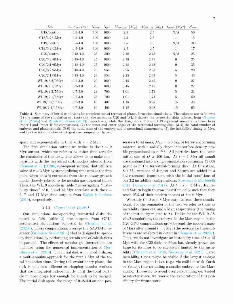
Table 2. Summary of initial conditions for complete sets of terrestrial planet formation simulations. The columns are as follows:(1) the name of the simulation set (note that the acronyms C20 and WL19 denote the terrestrial disks inferred from Clementet al. (2020a) and Walsh & Levison (2019), respectively, while the designators C18 and C19 represent simulations taken fromPaper I and Paper II for comparison), (2) the inner and outer edges of the terrestrial forming disk, (3-4) the total number ofembryos and planetesimals, (5-6) the total mass of the embryo and planetesimal components, (7) the instability timing in Myr,and (8) the total number of integrations comprising the set.

space and exponentially in time with τ = 2 Myr.

The first simulation output we utilize is the t = 2

Myr output, which we refer to as either time zero for

the remainder of this text. This allows us to make com-

parisons with the terrestrial disk models inferred from

Clement et al. (2020a, subsequent section) that utilize a

value of τ = 3 Myr by standardizing time zero as the first

point when data is extracted from the runaway growth

model (loosely related to the nebular gas dispersal time).

Thus, the WL19 models in table 2 investigating “insta-

bility times” of 0, 5 and 15 Myr correlate with the t =

2, 7 and 17 Myr time outputs from Walsh & Levison

(2019), respectively.

2.4.2. Clement et al. (2020a)

Our simulations incorporating terrestrial disks de-

noted as C20 (table 3) use outputs from GPU-

accelerated simulations reported in Clement et al.

(2020a). These computations leverage the GENGA inte-

grator (Grimm & Stadel 2014) that is designed to speed-

up simulations by performing certain sets of calculations

in parallel. The effects of nebular gas interactions are

included using the numerical implementation of Mor-

ishima et al. (2010). The initial disk is modeled utilizing

a multi-annulus approach for the first 1 Myr of the to-

tal simulation time. During this evolutionary phase, the

disk is split into different overlapping annular sections

that are integrated independently until the total parti-

cle number drops low enough for annuli to be merged.

The initial disk spans the range of 0.48-4.0 au and pos-

sesses a total mass, Mtot = 5.0 M⊕ of terrestrial forming

material with a radially dependent surface density pro-

file proportional to r−3/2. All particles have the same

initial size of D ' 200 km. At t = 1 Myr all annuli

are combined into a single simulation containing 43,608

particles in the terrestrial-forming disk. At this stage,

8.0 M⊕ versions of Jupiter and Saturn are added in a

3:2 resonance (consistent with the initial conditions of

our 3:2 instability configurations: Nesvorny & Morbidelli

2012; Deienno et al. 2017). At t = τ = 3 Myr, Jupiter

and Saturn begin to grow logarithmically such that they

reach 95% of their modern masses at t = 6 Myr.

We study the 3 and 8 Myr outputs from these simula-

tions. For the remainder of the text we refer to these as

instability times of 0 and 5 Myr, respectively (the timing

of the instability related to τ). Unlike for the WL19 LI-

PAD simulations, the embryos in the Mars region in the

C20 GPU computations grow beyond the modern mass

of Mars after around t = 5 Myr (the reasons for these dif-

ferences are analyzed in detail in Clement et al. 2020a).

Thus, we do not investigate an instability time of t = 15

Myr with the C20 disks as Mars has already grown too

large for its mass to be effectively limited by the insta-

bility (Clement et al. 2018; Nesvorny et al. 2021). Later

instability times might be viable if the largest embryo

in the Mars-region is lost (e.g.: via collision with Earth

or Venus), thus stranding a smaller embryo as the Mars

analog. However, to avoid overly-expanding our tested

parameter space, we reserve the exploration of this pos-

sibility for future work.

8

0.01

0.10

0.25

Mas

s (M

⊕)

0 Myr Embryo DistributionsControl (C18/C19)C20WL19

0.0 0.5 1.0 1.5 2.0 2.5 3.0 3.5 4.0

Semi-Major Axis (au)

0.01

0.10

0.25

Mas

s (M

⊕)

5 Myr Embryo Distributions

Figure 2. Comparison of embryo distributions for variousdisks tested in this manuscript. The acronyms C20 (blackpoints) and WL19 (green points) denote the terrestrial disksinferred from Clement et al. (2020a) and Walsh & Levison(2019), respectively, while the designators C18 and C19 (greypoints) represent simulation results taken from Paper I andPaper II for comparison. The top panel represents the stateof each disk at t = 0 Myr; the gas dispersal time. Conversely,the bottom panel plots the conditions of the same disks att = 5 Myr. The C18/C19 points in the top panel are exampleinitial conditions for control simulations from the respectiveworks, where as the similar points in the bottom panel are anexample embryo distribution from a C19 control simulationat t = 5 Myr (for an example of the state of the terrestrialdisk prior to an instability triggered at the 5 Myr point inthat work).

2.4.3. Disk Interpolation

We import our embryo distributions (table 2) directly

from all terrestrial objects with M ≥ 0.01 M⊕ in the

relevant simulation output files. Figure 2 plots these

distributions for the 0 and 5 Myr instability cases, along

with the “classic” disk conditions (Chambers & Wether-

ill 1998; Raymond et al. 2009) supposed in control sim-

ulations from Paper I and Paper II used as compari-

son cases throughout the analysis sections of this paper

(see section 2.4.4). The various instability times and

different disk models interrogated in this work should

be interpreted as different possible evolutionary states

the terrestrial disk might have attained around the time

of the instability’s onset (in terms of the total num-

ber of embryos and their cumulative masses). In this

paradigm, it is important to note that the major dif-

ference between our WL19 and C20 disks is the more

advanced evolutionary nature of the C20 models. This

is partially a consequence of the fact that we extract

data from the original C20 GENGA simulations at a

later epoch (t = 3 Myr) than for the WL19 LIPAD

models (t = 2 Myr). Moreover, the Walsh & Levison

(2019) simulations incorporate algorithms designed to

account for the effects of collisional fragmentation, thus

potentially limiting the efficiency of runaway growth

(Chambers 2013). Indeed, embryos in the Earth and

Venus-forming regions of our C20 models already pos-

sess masses of ∼0.3-0.4 M⊕ around the time of gas disk

dispersal (figure 2). In all simulations, embryos interact

gravitationally with all other objects in the system.

We generate planetesimal populations for our simula-

tions by randomly sampling the mass-weighted distribu-

tions of objects with M < 0.01 M⊕ in the WL19 and

C20 output files such that the in-situ mass distribution

(largely consistent with the original r−3/2 profile in both

cases) is roughly maintained (Birnstiel et al. 2012). Each

time a simulation is re-started (i.e.: after an unsuccessful

instability as described in section 2.2) a new planetesi-

mal population is selected and paired with a new, ran-

domly selected giant planet configuration. Thus, each

simulation combines a common embryo population (de-

pending on the specific simulation set: figure 2) with

a unique outer solar system and a unique planetesimal

population. In all simulations, planetesimals only feel

the gravitational effects of the embryos and giant plan-

ets. It should be noted here that our method of extract-

ing simulation outputs from the WL19 LIPAD and C20

GENGA simulations to pair with separate outer solar

system configurations imposes an artificial step change

on the giant planets’ semi-major axes and masses. While

this is a necessary simplification in our case, it limits the

robustness of our results, and future endeavors should

strive to more accurately model the transition from the

nebular gas phase of evolution to the epoch of giant im-

pacts.

We distribute 1,000 equal-mass planetesimals in our

t = 0 Myr instability simulations such that the total

mass in planetesimals is equal to the total mass of all ob-

jects with M < 0.01 M⊕ in the original GENGA and LI-

PAD simulations (column 6 of table 2). Therefore, plan-

etesimals in our integrations investigating WL19 disks

have initial masses of 0.00245 M⊕, and those in C20

models possess masses of 0.00243 M⊕ (Mpln). In order

to make accurate comparisons between our simulations

9

testing different instability times that are not compli-

cated by differences in individual planetesimal masses,

we maintain the values of Mpln from our 0 Myr insta-

bility runs in the 5 and 15 Myr instability sets. Thus,

disks constructed for the 5 and 15 Myr instability simu-

lations necessarily possess fewer planetesimals as a result

of their more advanced evolutionary states. This also

explains the broad differences between the total num-

ber of fully evolved systems we produce from each set of

initial conditions (last column of table 2). Simulations

investigating 5 and 15 Myr instability delays require less

compute time to complete than the 0 Myr batches by

virtue of beginning with fewer particles. Similarly, our

2:1 Jupiter-Saturn configurations yield successful insta-

bilities more regularly (Clement et al. 2021b), and thus

require fewer “restarts” to generate a fully evolved sys-

tem. It follows then that our WL19/2:1/15Myr set gen-

erates the largest sample of evolved systems. An alter-

native means of interpolating planetesimal populations

would be to assign each object a different mass that is

commensurate with the original simulations’ resultant

size frequency distribution, and we plan to explore the

effects of different planetesimal distributions further in

future work.

2.4.4. Reference Cases

We reference simulations of the classic model of ter-

restrial planet formation (both with and without a gi-

ant planet instability: Chambers & Wetherill 1998; Ray-

mond et al. 2009; Clement et al. 2018) throughout our

manuscript. These simulation batches are summarized

at the top of table 2. Disks denoted C18 (figure 2) are

derived from Paper I, and incorporate 100 equal-mass

embryos and 1,000 planetesimals, a surface density pro-

file proportional to r−3/2, and a total disk mass of 5.0

M⊕. Disks labeled C19 (Paper II) are identical to the

C18 disks, however these simulations are run using an

algorithm that accounts for fragmenting and hit-and-run

collisions (Leinhardt & Stewart 2012; Stewart & Lein-

hardt 2012; Chambers 2013). Otherwise, the numerical

methodology for both control sets is identical to that

described in this paper. In sets labeled “control” cases,

Jupiter and Saturn are included in their pre-instability,

3:2 MMR configuration for the entire 200 Myr integra-

tion. Additionally, we reference simulations from each

work (C18/3:2/1Myr and C19/3:2/1Myr) that include

a giant planet instability (the same 3:2 case tested here:

table 1) at t = 1 Myr; the most successful instability

time that is common to both works. While we only

present instability simulations from these papers that

finish with PS/PJ < 2.8 (as described in section 2.2), it

is important to note that these models possess a broader

range of final giant planet eccentricities than in our con-

temporary simulations. Finally, simulations designated

C20/control study the C20/0Myr disks (section 2.4.2)

without a giant planet instability model (Jupiter and

Saturn are instead modeled in a 3:2 resonance).

2.5. Success Criteria

We adopt the same success criteria (and alpha-

numeric designators) utilized in Paper I and Paper II

for consistency. These constraints are summarized in

table 3. Criterion A analyzes the bulk radial mass dis-

tribution of the final system of terrestrial planets. In our

classification algorithm, all objects with M > 0.05 M⊕are considered planets (note that we largely neglect Mer-

cury’s formation: Clement et al. 2019a, 2021a; Clement

& Chambers 2021), and all other remaining terrestrial

objects are referred to as left-over embryos and plan-

etesimals. To satisfy criterion A, a system must finish

with exactly two planets (Earth and Venus analogs) with

m > 0.6 M⊕ and a < 1.3 au, at least one planet (Mars

analog) with m < 0.3 M⊕ and 1.3 < a < 2.0 au (approx-

imately between Mars’ modern pericenter and the inner

edge of the asteroid belt), and no planets with m > 0.3

M⊕ and a > 1.3 au. However, to first order, an instabil-

ity simulation might still be successful if Mars finishes

with M < 0.05 M⊕, a > 2.0 au, or if the system possess

no Mars analog at all (see further discussion in Paper I).

For these reasons, and to prevent over-constraining our

simulations with criterion A, we report these three types

of systems (no Mars, Mars too small, Mars in asteroid

belt) as successful with criterion A1, provided the Earth

and Venus analogs still satisfy the constraints described

above.

Criteria B and C scrutinize the relative formation

timescales of Earth and Mars analogs. As in Papers

I and II, Earth analogs are defined as the largest object

in each simulation with 0.85 < a < 1.3 au and m > 0.6

M⊕, and Mars analogs comprise the largest planets in

each system with 1.3 < a < 2.0 au, regardless of classi-

fication in terms of A. Isotopic dating of lunar samples

indicate that the final major accretion event on Earth

(the Moon-forming impact) occurred ∼30-100 Myr after

nebular gas dissipation (Yin et al. 2002; Wood & Halli-

day 2005; Touboul et al. 2007; Kleine et al. 2009; Rudge

et al. 2010; Zube et al. 2019), although Earth’s formation

timescale and the timing of the Moon-forming giant im-

pact is still a topic for debate (e.g.: Barboni et al. 2017;

Thiemens et al. 2019). Conversely, analyses of the Mar-

tian meteorites suggest that Mars’ formation was com-

plete within just a few Myr of gas dispersal (Nimmo &

Agnor 2006; Dauphas & Pourmand 2011; Kruijer et al.

2017; Costa et al. 2020). In order to assess a system’s

ability to reproduce these bifurcated accretion histories,

criterion B requires that our Mars analogs accrete 90%

of their final mass by t = 10 Myr (relative to the gas

dispersal time). Conversely, to be successful in terms of

10

Code Criterion Actual Value Accepted Value Justification

A aMars 1.52 au 1.3-2.0 au Sunward of AB

A MMars 0.107 M⊕ ≥ 0.05,< .3M⊕ (Raymond et al. 2009)

A1 MMars 0.107 M⊕ ≥ 0.0,< .3M⊕ (Raymond et al. 2009)

A,A1 MV enus 0.815 M⊕ >0.6 M⊕ Within ∼ 25%

A,A1 MEarth 1.0 M⊕ >0.6 M⊕ Match Venus

B τMars 1-10 Myr <10 Myr (Kleine et al. 2009)

C τ⊕ 50-150 Myr >50 Myr (Dauphas & Pourmand 2011)

D MAB ∼ 0.0004 M⊕ No embryos (Chambers 2001)

E ν6 ratio Not used here

F WMF⊕ Not used here

G AMD 0.0018 <0.0036 (Raymond et al. 2009)

Table 3. Summary of success criteria for the inner solar system from Paper I and Paper II (a reproduction of table 3 fromeach respective work). The rows are: (1) the semi-major axis of Mars, (2-4) The masses of Mars, Venus and Earth, (5-6) thetime for Mars and Earth to accrete 90% of their mass, (7) the final mass of the asteroid belt, (8) the ratio of asteroids aboveto below the ν6 secular resonance between 2.05-2.8 au, (8) the water mass fraction of Earth, and (9) the angular momentumdeficit (AMD) of the inner solar system.

criterion C an Earth analog must take longer than 50

Myr to reach 90% of its ultimate mass.

A detailed analysis of the dynamical evolution of the

asteroid belt is beyond the scope of this manuscript (see:

Deienno et al. 2018; Clement et al. 2019c, 2020b, for

studies of the early instability scenario’s consequences

in the belt). However, a first order assessment of the

instability’s ability to adequately deplete the belt can

be made by scrutinizing the left-over particles in the

asteroid belt. As planetesimals do not grow through

collisions or feel the gravitational effects of one another

in our simulations, they can be viewed as tracers of the

more numerous planetesimals that actually populated

the primordial belt. For this reason, criterion D simply

requires that our simulations finish with no surviving

embryos or planets in the asteroid belt (2.0 < a < 4.0

au Chambers 2001; Chambers & Wetherill 2001) as these

objects would fossilize gaps in the belt’s orbital distri-

bution that are not observed today (Petit et al. 2001;

O’Brien et al. 2007; Raymond et al. 2009; Izidoro et al.

2016).

In Paper I and Paper II we analyzed the orbital archi-

tectures of our remnant asteroid belts by requiring that

systems possess more asteroids in the inner belt with

inclinations below the ν6 secular resonance than above

it (criterion E, the ratio in the actual belt is ∼0.08:

Walsh & Morbidelli 2011). Recent work in Clement

et al. (2020b) demonstrated that the giant planets’ resid-

ual migration phase (i.e.: migration after the instability)

largely sculpts the distribution of asteroidal inclinations

about ν6. Therefore, we do not utilize criterion E in our

current investigation. Similarly, criterion F assessed the

bulk volatile content of Earth analogs in Paper I and

Paper II. As our contemporary systems derive initial

conditions by sampling planetesimal populations from

Walsh & Levison (2019) and Clement et al. (2020a), the

connection between objects accreted by Earth analogs

and their original formation locations within the pri-

mordial nebula is not clearly defined. Therefore, we do

not consider criterion F in our present manuscript.

The low orbital eccentricities and inclinations of Earth

and Venus in the modern solar system also represent key

constraints for our simulations. The dynamical excita-

tion of a system of planets is typically quantified by its’

angular momentum deficit (AMD: Laskar 1997; Cham-

bers 2001); a measure of a system’s deviation from a

perfectly circular, co-planar collection of orbits:

AMD =

∑imi√ai[1−

√(1− e2i ) cos ii]∑

imi√ai

(1)

As in Paper I and Paper II, we require our terres-

trial systems (all planets with m > 0.05 M⊕) finish with

AMD < 2AMDSS (criterion G: Raymond et al. 2009);

where AMDSS is the modern statistic for the four ter-

restrial planets (0.0018).

3. RESULTS

3.1. Comparison with Past Work

The major conclusion of our investigation is that, to

first order, our new instability simulations (C20 and

WL19) produce qualitatively similar outcomes to the

models of Paper I and Paper II. This is particularly en-

couraging given that, in the absence of a giant planet in-

stability model, the WL19 and C20 disks (that presum-

ably represent more authentic initial conditions for the

giant impact phase) produce too many planets, overly

massive Mars analogs, and undersized Earth and Venus

analogs. Figure 3 plots the final masses and semi-major

axes of all planets formed in each of our different simula-

11

0.1

0.5

1.0

C18/control C19/control C20/control

0.1

0.5

1.0

C18/3:2/1Myr C19/3:2/1Myr C20/3:2/0Myr

0.1

0.5

1.0

Mas

s (M

⊕)

C20/2:1/0Myr C20/3:2/5Myr C20/2:1/5Myr

0.1

0.5

1.0

WL19/3:2/0Myr WL19/2:1/0Myr WL19/3:2/5Myr

0.5 1.0 1.5 2.00.1

0.5

1.0

WL19/2:1/5Myr

0.5 1.0 1.5 2.0

Semi-Major Axis (au)

WL19/3:2/15Myr

0.5 1.0 1.5 2.0

WL19/2:1/15Myr

Figure 3. Distribution of semi-major axes and masses for all planets formed in all simulation sets. The red squares denote theactual solar system values for Mercury, Venus, Earth and Mars. The vertical dashed line separates the Earth and Venus analogs(left side of the line) and the Mars analogs (right side). Details on the two instability models are tabulated in table 1 and theinitial disk conditions for each set are summarized in table 2.

12

tion batches (table 2). Indeed, the Mars analog masses

(all planets with a > 1.3 au) in all of our instability

batches are consistently less than those in our three con-

trol sets. Moreover, no Mars analog in an instability

simulation finishes with M > 1.0 M⊕ (we elaborate fur-

ther on the instability’s tendency to stunt Mars’ growth

in section 3.1.1).

It is clearly apparent from these plotted distributions

that the WL19 disks systematically struggle to form suf-

ficiently massive Earth and Venus analogs. These dif-

ferences are easily understood by inspecting the initial

mass profile in each disk model. The WL19 disks are

comprised of 3.32 M⊕ of planet forming material be-

tween 0.7 and 3.0 au, with initial planetesimal semi-

major axes selected such that the disk surface density

profile falls off proportional to r−3/2. Thus, these disks

nominally contain ∼1.13 M⊕ of terrestrial-forming ma-

terial with a < 1.3 au at time zero. In order to form

adequate Earth and Venus analogs and satisfy criteria

A and A1, the respective analogs’ feeding zones must

stretch well into the Mars-forming region. While it is

common for Earth-analogs in classic N-body studies of

terrestrial planet formation to accrete a significant frac-

tion of objects from the outer regions of the disk (Ray-

mond et al. 2007; Fischer & Ciesla 2014; Kaib & Cowan

2015), the instability’s tendency to void this region of

large embryos conspires to severely limit the availability

of such material in our WL19 instability runs. Thus,

while these simulations are successful in terms of sup-

pressing the distribution of masses outside of ∼1.3 au,

the analog systems themselves tend to provide poor

matches to the actual system of terrestrial planets in

terms of the masses of Earth and Venus (the majority

of M > 1.0 M⊕ planets occur in simulations that only

form a single planet with a < 1.3 au).

The tendency of WL19 disks to form under-mass ver-

sions of Earth and Venus is slightly mitigated in our

simulation batches investigating later instability delay

times of 5 and 15 Myr. Indeed, these batches are the

only WL19 simulations in our sample to satisfy criteria

A or A1, with the former (5 Myr) being more success-

ful in terms of consistently yielding small Mars analogs

(i.e.: the instability occurs before Mars grows too large:

Clement et al. 2018; Nesvorny et al. 2021). In such real-

izations, Earth and Venus are able to accrete a sufficient

quantity of material from the outer disk prior to the in-

stability reshaping the asteroid belt and Mars-forming

region. These results are best interpreted as favoring the

instability’s transpiration at an epoch where the terres-

trial disk has attained an evolutionary state similar to

our WL19/5Myr initial conditions; with roughly half the

disk mass distributed in smaller planetesimals, and the

remaining half locked in larger embryos (table 2).

In contrast to the WL19 models, our C20 disks begin

with a total mass of terrestrial-forming material equal

to 5.0 M⊕, distributed between 0.48 and 4.0 au with a

surface density profile that is proportional to r−3/2 (our

reference C18 and C19 simulations essentially employ

an identical disk in terms of its total mass and radial

extent). Therefore, our C20 simulations are initialized

with ∼1.7 M⊕ of planet forming material in the Earth

and Venus-forming regions (a <1.3 au); roughly equiva-

lent to the modern cumulative mass of the two planets

(1.815 M⊕).

Figure 3 does not evince substantial differences

between the distribution of planets formed in our

C20/0Myr and C20/5Myr instability models. This is

not particularly surprising, given the fact that the ratio

of total embryo to planetesimal mass does not mean-

ingfully evolve between 0 and 5 Myr in the original C20

GENGA simulations. Instead, the largest difference be-

tween the two models is the actual masses of the larger

embryos in the Earth and Venus-forming region (figure

2). Indeed, Clement et al. (2020a) noted that these em-

bryo configurations emerge from the gas disk phase in

a substantially-evolved, quasi-stable configuration that

tends to hinder subsequent accretion events (note that

our reference C20/control simulations finish the 200 Myr

giant impact phase with 6.4 planets per system). How-

ever, this is clearly not a problem in our C20 models

that include a giant planet instability model as, to first

order, the results of all four simulation batches (in terms

of criterion A1 and the distributions depicted in figure

3) are largely consistent with those of the C18 and C19

reference instability simulations. The largest outlier of

our four C20 instability batches in terms of criterion

A and A1 is the C20/3:2/5Myr set, however we as-

sess these discrepancies to largely be the consequence

of small number statistics (the set only yields 20 total

systems), rather than a systematic shortcoming of the

3:2 instability model. Thus, our results indicate that a

smaller number of more massive embryos in the Earth

and Venus-forming regions around the time of nebular

gas dissipation is a viable initial configuration for the

early instability scenario. While the cosmochemical im-

plications of this scenario remain to be explored (e.g.:

the consequences for differentiation, volatile delivery,

volatile retention, etc.), bridging the gap between the

runaway growth simulations of Walsh & Levison (2019)

and Clement et al. (2020a) and the modern terrestrial

system is an encouraging finding of our present investi-

gation. We explore the causes of lower order variances

in outcomes in the subsequent sections.

3.1.1. Stunting Mars’ growth

Our simulations confirm the results of Paper I and Pa-

per II and broadly evidence the Nice Model instability’s

capacity to substantially restrict Mars’ growth. Figure 4

13

Set A A1 B C D G

a,mTP mTP τMars τ⊕ MAB AMD

C18/control 0 0 9 86 2 8

C18/3:2/1Myr 26 26 12 95 20 14

C19/control 2 2 33 80 2 15

C19/3:2/1Myr 35 35 23 80 70 12

C20/control 0 0 0 57 5 75

C20/3:2/0Myr 12 20 45 28 72 15

C20/2:1/0Myr 8 20 39 37 66 17

C20/3:2/5Myr 0 5 50 33 95 0

C20/2:1/5Myr 11 27 45 35 75 12

WL19/3:2/0Myr 0 0 5 60 89 48

WL19/2:1/0Myr 0 0 7 0 86 40

WL19/3:2/5Myr 4 9 23 57 77 23

WL19/2:1/5Myr 4 6 42 54 88 19

WL19/3:2/15Myr 0 2 N/A 37 68 3

WL19/2:1/15Myr 0 0 N/A 27 82 6

Table 4. Summary of percentages of systems which meet the various terrestrial planet success criteria established in table3 (reference simulation statistics are reproduced from: Clement et al. (2018, Paper I) (C18), Clement et al. (2019b, PaperII) (C19), and Clement et al. (2020a) (C20)). The subscripts TP and AB indicate the terrestrial planets and asteroid beltrespectively.

plots the cumulative distribution of Mars analog masses

in the various simulation sets from this study, and sev-

eral reference models from our previous work (table 2).

The similarity between the three blue curves (control

runs without an instability), in addition to the consis-

tency of the instability curves (green, black and grey

lines) clearly demonstrates the transparency of Mars’

formation to the particular terrestrial disk utilized (C18,

WL19 or C20) and instability model employed (2:1 or

3:2). It should be noted here that, given the resolution

of our simulations, we intentionally plot all Mars analogs

with M < 0.05 M⊕ as possessing no mass.

The largest difference between the five instability

curves in figure 4 is the over-abundance of ∼0.05-

0.08 M⊕ Mars analogs in the C18/3:2/1Myr and

C19/3:2/1Myr reference simulations compared to our

contemporary instability models. We attribute these

variances to the relative absence of embryos in this mass

range within the Mars-forming region at the time of the

instability in the WL19 and C20 disks (figure 2). As

the largest embryos in the Mars-forming region of these

disks already possess masses close to that of the real

planet, it makes sense that few simulations yield smaller

versions of the planet.

Our new instability simulations possess systematically

improved success rates for criterion D (i.e.: they do

not strand embryos in the asteroid belt) compared to

the reference instability simulations from Paper I and

Paper II. There are two important factors responsible

for these differences. First, our new results are derived

from an increased fraction of systems with adequately

excited values of eJ compared to our previous simula-

tion batches (by virtue of our numerical pipeline: section

2.2). Clement et al. (2019c) demonstrated a positive cor-

relation between eJ and total depletion in the asteroid

belt. It therefore follows that &70% of the runs in each

of our simulation batches completely erode the asteroid

belt region of larger embryos. Second, our simulations

are initialized with a small number embryos in the aster-

oid belt. Our WL19 models only possess a few embryos

with semi-major axes just inside of 2.0 au (see figure 2),

and our C20 disks contain a system of five, ∼0.02 M⊕embryos in the belt. This is the consequence of the time

required to reach the analytical isolation mass via run-

away growth in the asteroid belt being much longer than

the nebular gas dissipation timescale (Kokubo & Ida

1996). Conversely, the reference C18 and C19 simula-

tions begin with ∼20, 0.025 M⊕ embryos in between 2.0

and 4.0 au. Thus, particles in the asteroid belts of the

WL19 LIPAD and C20 GENGA simulations simply

are not permitted sufficient time to collisionally assem-

ble and form an evolved, bimodal population of embryos

and planetesimals. As a result of utilizing these more

realistic initial conditions in our contemporary study,

we only note 15 examples of planets more massive than

Mars forming in the asteroid belt within our entire batch

of 356 instability simulations.

More massive Mars analogs loosely correlate with

shorter instability delay times (i.e. 0 Myr vs. 5 and

15 Myr) for both the C20 and WL19 simulation batches

14

10-1 100

MMars (M⊕)0.0

0.2

0.4

0.6

0.8

1.0

Cum

ulat

ive

Frac

tion

Actual MarsC18/controlC19/controlC20/controlC18+C19/1MyrC20/0MyrC20/5MyrWL19/0MyrWL19/5+15Myr

Figure 4. Cumulative distribution of Mars analog massesformed in our various simulation sets from this manuscript(black and green lines) compared with reference (see table 2)simulation batches from Clement et al. (2018, 2019b, 2020a).Systems plotted in shades of blue represent simulations thatdid not incorporate a giant planet instability model fromeach respective past work. The transparent thick grey linecombines the 1 Myr instability delay reference simulations:C18/3:2/1Myr and C19/3:2/1Myr. Black lines correspond toC20 disk simulations from this work, and green lines denoteWL19 disk runs. The solid and dashed lines for each dataset separate 0 Myr instability delay simulations (solid) fromthe 5 and 15 Myr (dashed) batches. The grey vertical linescorresponds to Mars’ actual mass. Note that some systemsmay form multiple planets in this region, but here we onlyplot the most massive planet. Systems that do not form aMars analog via embryo accretion (i.e.: MMars < 0.05 M⊕)are plotted as having zero mass.

depicted in figure 4. This result is also evident in the

distributions of planets plotted in figure 3. Similarly,

our C20/0Myr simulations possess lower success rates

for criterion D than the C20/5Myr models. Paper I an-

alyzed these trends in detail and concluded that instabil-ities ensuing precipitously from less-processed terrestrial

disks were less successful as the disk tends to re-spread

after being truncated by the instability through inter-

actions between embryos and overly-abundant planetes-

imals. When this is the case, fully evolved systems of-

ten contain 3-4 similarly massed planets. Thus, Mars

analogs tend to be too massive, while Earth and Venus

are too small. However, both the WL19 and C20 disks

tested in our current study attain advanced evolution-

ary states around the time of nebular gas dissipation.

As a result, these trends are not as pronounced as in

Paper I and Paper II. Specifically, this is a result of

the fact that the embryo-planetesimal mass partition-

ing in the Mars-forming region is similar in all of our

simulation sets (roughly half of the mass in embryos

and half in planetesimals). Thus, we conclude that all

three timings (0, 5 and 15 Myr) investigated in our cur-

rent work are viable in terms of consistently replicating

0.0

0.1

0.2

0.3t=0: Dispersal of the gas disk.

0.0

0.1

0.2

0.3t=500 Kyr: The instabilityinitiates

0.0

0.1

0.2

0.3

Ecce

ntric

ity t=10 Myr: Mars growthcomplete. Earth and Venusstill forming.

0.0

0.1

0.2

0.3t=200 Myr: Final state of thesystem.

1 10

Semi-Major Axis (au)0.0

0.1

0.2

0.3

0.4Present Solar System.

Figure 5. Semi-Major Axis/Eccentricity plot depicting theevolution of a successful system in the C20/2:1/5Myr batch.The size of each point corresponds to the mass of the particle(because Jupiter and Saturn are hundreds of times more mas-sive than the terrestrial planets, we use separate mass scalesfor the inner and outer planets). For reference, the embryothat becomes the Mars analog is plotted in red. The finalterrestrial planet masses are MV enus = 0.88 (MV enus,SS =0.815), MEarth = 0.92 and MMars = 0.18 (MMars,SS =0.107) M⊕. The additional surviving embryo in the Marsregion has a mass of 0.04 M⊕ (we extended this simulationand found that the embryo collided with the Sun at t = 285Myr). This simulation also satisfies the four success criteriafor the giant planets (e55 = 0.023, PS/PJ = 2.36; comparedwith e55,ss = 0.044, PS/PJ,ss = 2.49) described in Nesvorny& Morbidelli (2012) and Clement et al. (2021b).

Mars’ mass. However, as discussed in the previous sec-

tion, constraints related to Earth and Venus’ mass lead

us to disfavor delays of 0 and 15 Myr for the WL19 disks.

Moreover, we do not test delays longer than 5 Myr with

our C20 disks as embryos in the Mars region grow too

massive after t ' 5 Myr. Figure 5 plots an example

successful evolution from our preferred C20/2:1/5Myr

batch of simulations.

3.1.2. Angular Momentum Deficit

Figure 5 highlights the challenge of replicating the low

orbital eccentricities and inclinations of Earth and Venus

in instability models that adequately excite the orbits

of the gas giants. Indeed, the Earth and Venus analogs

in this simulation each possess e ' 0.10; substantially

more dynamically excited than the nearly circular or-

bits they inhabit in the actual solar system. Figure 6

15

plots the cumulative distribution of AMDs in our var-

ious simulation sets, compared with those of systems

formed in our reference simulations from Paper I, Paper

II and Clement et al. (2020a). In general, our instability

simulations yield a fraction of systems with AMDs less

than twice the solar system value (table 4) that is sim-

ilar to those formed in control disks with an instability

model (though the median values are clearly different:

blue lines in figure 6). Moreover, we note no significant

differences in the final AMDs produced in simulations

invoking different giant planet instability models (2:1

and 3:2; see table 1). This demonstrates that pertur-

bations from the strong ν5 resonance being initialized

closer to the Earth-forming region in our 2:1 models do

not adversely affect the final distribution of AMDs.

While the angular momentum deficit of the terrestrial

system is still a problem in our new models, our con-

temporary results are no worse than those of our pre-

vious models. As our simulation pipeline (section 2.2)

is specifically designed to select for stronger instabil-

ity that yield higher gas giant eccentricities, one might

naively expect our new instabilities to systematically

possess larger AMDs than the C18/1Myr and C19/1Myr

reference models. However, our contemporary integra-

tions actually perform about the same or, in certain

cases, slightly better when measured against criterion

G. Indeed, all four 0 Myr delay simulation batches boast

higher success rates for G and marginally-improved dis-

tributions of AMDs in figure 6. It is therefore likely

that this improvement (or lack of retrogression) is re-

lated to the structure of the WL19 and C20 disks them-

selves. This is supported by the fact that 75% of our

C20/control simulations satisfy criterion G. Embryos in

the Earth and Venus-forming region of the WL19 and

C20 disks attain relatively large masses (figure 2) while

still engulfed in the dense nebular gas. As a result, the

embryos emerge from the gas disk on dynamically cold

orbits, and require only a few additional large accretion

events to reach their final masses (section 3.1.3). As

these embryos experience fewer large encounters that

might excite their eccentricities in these more processed

terrestrial disks, they tend to survive the planet forma-

tion process with lower eccentricities and inclinations

than the Earth and Venus analogs in our C18 and C19

reference models.

While the solar system outcome lies comfortably

within the lower range of AMDs generated in all of

our various instability simulations (green and black lines

of figure 6), this result is potentially misleading since

overly-massive Mars analogs with low eccentricities can

positively modify the AMDs of systems with overly-

excited Venus and Earth analogs towards successful val-

ues. Given the preponderance of systems that resemble

the one plotted in figure 5, we conclude that the repli-

100 101

AMD/AMDSS

0.0

0.2

0.4

0.6

0.8

1.0

Cum

ulat

ive

Frac

tion

AMDSS

C18/controlC19/controlC20/controlC18+C19/1MyrC20/0MyrC20/5MyrWL19/0MyrWL19/5+15Myr

Figure 6. Cumulative distribution of AMDs (normalizedto the solar system value for the four terrestrial planets:equation 1) formed in the various simulation sets from thismanuscript (black and green lines) compared with referencesimulation batches from Clement et al. (2018, 2019b, 2020a,see table 2). Systems plotted in shades of blue representsimulations that did not incorporate a giant planet insta-bility model. The transparent thick grey line combines the1 Myr instability delay reference simulations C18/3:2/1Myrand C19/3:2/1Myr. Black lines correspond to C20 disk in-stability simulations from this work, and green lines denoteWL19 disk runs. The solid and dashed lines for each dataset separate 0 Myr instability delay simulations (solid) fromthe 5 and 15 Myr (dashed) batches.

cation the low AMD of the modern terrestrial system

represents a significant outstanding problem for future

models to resolve. In addition to focusing on the par-

ticularly problematic eccentricities and inclinations of

Earth and Venus (rather than the entire terrestrial sys-

tem: Nesvorny et al. 2021), such investigations should

comprehensively attempt to account for imperfect col-

lisions (Chambers 2013; Clement et al. 2019b; Deienno

et al. 2019) and the effects of the dissipating gas disk

(e.g.: Morishima et al. 2010; Matsumura et al. 2010; Lev-

ison et al. 2015b; Carter et al. 2015).

3.1.3. Fewer Giant Impacts

Earth analogs in our simulations typically reach their

final masses within the first ∼50 Myr following the in-

stability’s onset via a final giant impact with a roughly

equal-mass impactor. This is not particularly surpris-

ing given the more advanced evolutionary states of the

Earth and Venus-forming regions in our WL19 and C20

disks at the beginning of our simulations. In all of

our simulation batches, this regime is dominated by 3-

5, ∼0.1-0.4 M⊕ embryos around the time of the Nice

Model’s onset. As a consequence of increased eccen-

tricity excitation in the inner solar system after the in-

stability, these large proto-planets precipitously attain

crossing orbits that lead then to quickly combine and

16

0.25

0.50

0.75

Venus Analog Accretion

0.25

0.50

0.75

M/M

f

Earth Analog Accretion

10-1 100 101 102

Time (Myr)

0.25

0.50

0.75

Mars Analog Accretion

Criterion B/C

0 Myr Instability

0.25

0.50

0.75

Venus Analog Accretion

0.25

0.50

0.75

M/M

f

Earth Analog Accretion

10-1 100 101 102

Time (Myr)

0.25

0.50

0.75

Mars Analog Accretion

Criterion B/C

5 Myr Instability

Figure 7. Accretion histories for analog planets in our various simulation sets investigating 0 and 5 Myr instability delays (leftand right panels, respectively, note that time zero correlates with the beginning of the simulation). Venus analogs (top panels)correspond to all planets with M > 0.6 M⊕ and a < 0.85 au; Earth analogs consists of planets with M > 0.6 M⊕ and 0.85< a < 1.3 au, while Mars analogs are defined as all objects with 0.05 < M < 0.3 M⊕ and 1.3 < a < 2.0 au. Each planet’smass is normalized to its final value and plotted as a function of time over the duration of the simulation. The red vertical linescorrelate with our success criteria B (<10 Myr with respect to time zero) and C (>50 Myr) for the respective growth timescalesof Mars and Earth analogs.

form Earth and Venus-analogs. Figure 7 depicts the ac-

cretion histories for all Earth (M > 0.6 M⊕; 0.85 < a <

1.3 au), Venus (M > 0.6 M⊕; a < 0.85 au) and Mars

(0.05 < M < 0.3 M⊕; 1.3 < a < 2.0 au) analog planets

formed in our various simulation sets. Table 5 sum-

marizes the same data, and provides the percentages of

analogs accreting 90% of their ultimate masses within

the first 10, 50 and 100 Myr following the instability

for each of our simulation batches investigating different

instability delays. Though the total fraction of Earth

analogs with growth timescales in excess of 50 Myr (cri-

terion C) in each of our simulation batches is less than

for the C18/3:2/1Myr and C19/3:2/1Myr reference sets,

a reasonable fraction of systems still experience late fi-

nal giant impacts that are consistent with the inferred

timing of the Moon-forming impact (Kleine et al. 2009;

Rudge et al. 2010; Kleine & Walker 2017).

We note that the prevalence of equal-mass final im-

pacts on Earth is potentially consistent with the Moon-

formation scenario envisioned in Canup (2012). While

these conditions are fairly improbable in the classic

terrestrial planet formation model (a ∼Mars-mass im-

pactor is far more common: Chambers & Wetherill 1998;

Kaib & Cowan 2015), they occur fairly regularly when

both our WL19 and C20 disks are perturbed by the gi-

ant planet instability.

In contrast to the formation of Earth, many of our

Venus analogs form within a few tens of Myr without ex-

17

tinst t90 < 10 Myr t90 < 50 Myr t90 < 100 Myr

0 Myr instabilities

Venus 13 53 84

Earth 0 58 84

Mars 23 48 8

5 Myr instabilities

Venus 15 65 84

Earth 11 57 83

Mars 48 84 96

15 Myr instabilities

Venus 16 65 93

Earth 20 70 85

Mars 47 84 94

Table 5. Summary of percentages of planet analogs accret-ing 90% of their ultimate mass within the first 10, 50 and 100Myr (columns 2-4) after the instability. Note that, in con-trast to our calculations for criterion B and C (the accretiontime with respect to time zero: table 3), here we computethe growth timescale with respect to the instability’s onset.

periencing a significant final giant impact. This result is

consistent with the dichotomous histories of Earth and

Venus proposed in Jacobson et al. (2017) to reconcile

Venus’ lack of an internally generated dynamo and nat-

ural satellite. Additionally, figure 7 and table 5 clearly

demonstrates the tendency of Mars analogs in our 0

Myr instability delay batches to experience prolonged

accretion histories (criterion B) that are inconsistent

with the planets’ inferred geological formation timescale

(Dauphas & Pourmand 2011; Kruijer et al. 2017). This

is a result of the disk re-spreading after the instability

(discussed in section 3.1.1). Conversely, the accretion

histories of our 5 Myr instability delay Mars analogs

(right panel of figure 7) and their corresponding success

rates for criterion B provide a better match to the actualplanets’ presumed rapid growth (an improvement from

our reference C18/3:2/1Myr and C19/3:2/1Myr insta-

bility sets from Papers I and II).

3.2. Jupiter’s eccentricity excitation

Our simulations indicate that the instability’s ten-

dency to sufficiently stunt Mars’ growth correlates with

the adequate excitation of Jupiter’s eccentricity towards

the solar system value. Figure 8 plots the relationship

between Mars’ mass and the excitation of Jupiter’s fifth

eccentric mode (e55,SS = 0.044; closely related to the

planets’ mean eccentricity in the modern solar system).

To determine e55, we integrate each remnant system of

planets for an additional 10 Myr and compute the sec-

ular frequencies and relative coefficients for each planet

via frequency modified Fourier transform (Sidlichovsky

& Nesvorny 1996). We also analyzed the connection

between MMars and the other eccentric modes of the

Jupiter-Saturn system and concluded that depletion in

the outer terrestrial disk correlates most strongly with

e55. As many of our instabilities over-excite Saturn’s

eccentricity (quantified here by its eccentric forcing on

Jupiter: e56,SS = 0.0157), we only display systems that

finish in the e55 > e56 regime (e.g.: Clement et al.

2021b). By substantially increasing our sample of sys-

tems with PS/PJ < 2.5, high e55, and low e56, our re-

sults reinforce the general trends observed in Paper I.

Outcomes where MMars & 0.3 M⊕ (criterion A) are al-

most exclusively derived from simulations that do not

properly excite e55. Exceptions to this trend are lim-

ited to WL19/0Myr runs where the instability occurs

too early; thus causing the remnant terrestrial disk to

spread and repopulate the Mars-forming region with em-

bryos and planetesimals from the Earth-forming region

(section 3.1.1).

While a statistical comparison between our 2:1 and

3:2 instability models (table 1) is complicated by our

simulation pipeline that restarts integrations that ex-

perience unideal jumps or excessive residual migration

(section 2.2), it is clear from figure 8 that our new 2:1

scenarios yield similar results to the 3:2 cases typically

considered in the literature. To crudely control for the

effects of our simulation pipeline, table 6 reports the per-

centage of simulations that effectively limit Mars’ mass

to less than that of the real planet from the subset of

all realizations where e55 is excited to at least 50% of

its modern value. 49% of all our 2:1 models are suc-

cessful in this manner, as compared with 57% of our

3:2 runs. If we increase our limiting value for Mars’

mass to 0.3 M⊕ (criterion A) 87% of our 2:1 simula-

tions and 92% of our 3:2 models adequately exciting e55possess a small Mars. Thus, while the subset of sim-

ulations that reasonably replicate Jupiter’s eccentricity

are highly successful at limiting Mars’ mass (regardless

of giant planet instability model employed), our 3:2 sets

tend to more efficiently restrict Mars’ growth.

Figure 8 demonstrates how Earth and Venus’ ability to

continue to accrete material after the instability and at-

tain the correct masses is not hindered when e55 is prop-

erly excited. The color of each point in the plot depicts

the total planetary mass in the Earth-Venus region (a <

1.3 au). Nominally this corresponds to the cumulative

mass of Earth and Venus when criterion A is satisfied,

however we include systems that form different numbers

of planets (i.e.: one ∼ 2.0 M⊕ planet, or three smaller

planets) to decouple the stochastic nature of the peculiar

series of final impacts that generates the Earth-Venus

system. The fact that multiple dark blue and purple

points fall within the grey shaded regions demonstrates

that the solar system result falls well within the spec-

trum of outcomes produced by our simulations. While

the low masses of Earth and Venus analogs in the 15

18

Myr instability delay simulations are related to features

of the WL19 disks discussed in 3.1.1, the prevalence of

light blue points throughout all panels of the figure ex-

poses the fragility of the terrestrial system during the

violent and stochastic Nice Model instability (e.g.: Ag-

nor & Lin 2012; Kaib & Chambers 2016). Indeed, many

simulations yield a residual terrestrial system that bares

little resemblance to the actual inner solar system if, for

example, the gas giants spend lengthy periods of time

on highly-eccentric orbits or the ejected ice giant makes

an inordinate number of perihelia passages through the

inner solar system. Similarly, the number of small Mars

analogs formed in simulations with excessively low final

e55 values evidences the stochasticity of the instability.

As our numerical pipeline (section 2.2, point 3) neces-

sarily selects for systems that attain high-eJ values dur-

ing the instability, these low-MMars/low-e55 outcomes

occur when the eccentricity excitation in the outer so-

lar system is sufficient (i.e.: the gas giants attain high

eccentricities for long enough) to significantly evacuate

material from the Mars-forming region before the giant

planets’ orbits damp excessively during the residual mi-

gration phase (e.g.: Nesvorny & Morbidelli 2012).

Nesvorny et al. (2021) argued that depletion in the

Mars and asteroid belt regions is fairly independent of

the giant planets’ peculiar evolution (i.e.: eccentricity

excitation during the instability, depth and duration of

encounters with the ejected planet, etc.). Rather, the

authors posited that the dominant mechanism responsi-

ble for limiting Mars’ mass is the giant planets’ attaining

non-zero eccentricities before Mars exceeds its modern

mass. Thus, the early instability scenario is essentially

an extension of the EEJS (Extra Eccentric Jupiter and

Saturn) model of Raymond et al. (2009). Regardless of

whether the giant planets originate on eccentric orbits,

or acquire them via an early Nice Model instability, the

results are qualitatively the same. Specifically, Nesvorny

(2021) studied three independent instability evolutions

(case 1 and 2 from Nesvorny et al. (2013) and the model

of Deienno et al. (2018)). However, these three instabil-

ities investigated by the authors transpired at dissimilar

epochs (6, 20 and 0.6 Myr, respectively), thus compli-

cating an interpretation of the effects of each particular

model. Our contemporary simulations largely confirm

the overall conclusions of Nesvorny et al. (2021). The

tendency of the instability to limit Mars’ mass correlates

most strongly with the adequate excitation of Jupiter’s

eccentricity. As all simulations that sufficiently excite

e55 finish with a small Mars, it is clear that the early

instability scenario is viable for a broad spectrum of

plausible evolutionary pathways for the giant planets;

provided the evolution culminates in a solar system-like

giant planet architecture.

10-2 10-1

0.1

0.5

0 Myr Instability Delay

10-2 10-1

0.1

0.5

MMars

(M⊕

)

5 Myr Instability Delay

10-2 10-1

e55 (Jupiter Eccentricity Excitation)

0.1

0.5

15 Myr Instability Delay

SS3:22:1

1.0 1.5 SS 2.0Mass in planets with a< 1.3 au (M⊕)

Figure 8. Dependence of depletion in the inner solar systemon Jupiter’s eccentricity excitation (quantified here by e55:the magnitude of the solar system’s fifth eccentric eigenfre-quency, g5, in Jupiter’s eccentricity). Only simulations withe56 < e55 are plotted (i.e. those that do not over-exciteSaturn). Each sub-panel displays results from our variousbatches of simulations investigating different instability de-lay times (0, 5 and 15 Myr: table 2). Each point plots Mars’final mass against e55 (Mars analogs with M < 0.05 M⊕ areplotted as possessing no mass). The color of each point cor-responds to the total remaining planetary mass with a < 1.3au (nominally Earth and Venus analogs). Simulations uti-lizing a 3:2 Jupiter-Saturn resonance instability model areplotted with circular points, and 2:1 models are assigned tri-angular markers. The stars plot the solar system values ofMMars and e55. The grey shaded regions encompass simu-lations with 0.05 < MMars < 0.3 M⊕ (criterion A) and e55within 50% of the solar system value (Clement et al. 2021b).

3.3. Residual migration beyond Jupiter and Saturn’s

5:2 MMR

An unanswered question from our previous investiga-

tions of the early instability scenario in Paper I and Pa-

per II centers around instability evolutions that achieved2.5 < PS/PJ < 2.8. Systems within this range were

19

Constraint 2:1 3:2

N(MMars ≤ 0.107) / N(e55 ≥ 0.022) 49 57

N(MMars ≤ 0.107) / N(PS/PJ ≤ 2.5) 49 34

N(MMars ≤ 0.107) / N(e55 ≥ 0.022 & PS/PJ ≤ 2.5) 47 47

Table 6. Summary of percentages of systems from our simulation batches investigating different instability models (2:1 and3:2; table 1) simultaneously satisfying important constraints for the inner and outer solar system. The rows are as follows: (1)percentage of all systems adequately exciting Jupiter’s eccentricity (e55 > 0.022) that produce a small Mars (MMars < 0.3 M⊕),(2) percentage of systems with PS/PJ < 2.5 that possess a small Mars, and (3) small Mars-hosting systems from the subset ofsimulations simultaneously successful in terms e55 and PS/PJ .

considered in both papers to attain adequate statistics

as outcomes where the gas giants finish inside of their

mutual 5:2 MMR are slightly uncommon in statistical

studies of the instability (only ∼17% of both our 2:1

and 3:2 models are successful in this manner2). As the

dominant secular resonances currently in the inner as-

teroid belt presumably perturb the Mars-forming region

more strongly in evolutions where PS/PJ exceeds the

modern value, it is unclear whether the incorporation of

these results in our previous work artificially boosted the

fraction of systems finishing with a small Mars. In the

modern asteroid belt, the zero-inclination, eccentricity-

averaged locations of the ν6 and ν16 resonances are at

∼ 2.05 and ∼ 1.95 au, respectively.

Figure 9 plots the mass of Mars against the final value

of PS/PJ in each of our various simulation sets (analogs

with MMars < 0.05 M⊕ and those forming no Mars ana-

log are depicted as possessing zero mass). As in figure 8,

the color of each point corresponds to the total mass in

planets with a < 1.3 au. In this manner, dark blue and

purple points falling in the grey shaded region delimiting

2.3 < PS/PJ < 2.5 and 0.05 < MMars < 0.3 should be

interpreted as successful in terms of truncating the ter-

restrial disk in the Mars-forming region without limiting

the accretion of the remaining inner planets. It is clear

from figure 9 that appropriate inner solar system mass

distributions occur across the full range PS/PJ values

produced in our simulations.

A loose trend of enhanced Mars and total Earth-Venus

masses appears to manifest around 2.4 . PS/PJ . 2.6,

near the solar system value of 2.49. Thus, the largest

final period ratios do tend to correlate with marginally

depressed Mars masses, however this is partially a con-

sequence of small number statistics and the fact that

these values are unlikely outcomes of our simulation

pipeline (section 2.2). While we cannot discount the

2 Note that the rarity of attaining PS/PJ < 2.5 in and of itselfis not a systematic issue in statistical studies of the Nice Modelas the solar system result is merely one possibility within a broadspectrum of final values of PS/PJ . However, the tendency ofPS/PJ < 2.5 instabilities to under-excite e55 is a systematic issuein the sense that the solar system result, while possible, is a sta-tistical outlier (particularly for the 3:2 instability: Clement et al.2021b).

fact that residual migration beyond Jupiter and Sat-

urn’s mutual 5:2 resonance likely artificially suppresses

the masses of Mars analogs, figure 9 depicts numerous

realizations that are exemplarily solar system analogs in

terms of simultaneously matching the mass distribution

in the terrestrial region and PS/PJ . As the solar system

result is clearly well within the spectrum of outcomes

produced in our simulations, we conclude that variances

resulting from the stochastic nature of terrestrial planet

formation and the Nice Model instability significantly

outweigh the effects of residual migration past PS/PJ =

2.5.

When we isolate systems finishing with PS/PJ , as in

section 3.2 (table 6), we find that our 2:1 models are

slightly more successful at restricting Mars’ growth than

the 3:2 simulations (49% versus 34% of simulations lim-

iting Mars’ mass to less than its actual value). These

trends essentially counterbalance the results discussed

in section 3.2 for simulations adequately exciting e55.

Thus, identical percentages (47%) of both our 3:2 and

2:1 simulations simultaneously attaining e55 > 0.022 and

PS/PJ < 2.5 also produce a Mars that is less massive

than the real planet (this statistic increases to 89% when

we consider Mars analogs withMMars < 0.3M⊕). Thus,

we conclude that the primordial 2:1 Jupiter-Saturn res-

onance is an equivalently viable initial condition (com-

pared to the 3:2) for the early instability scenario.

3.4. Mercury Analogs

In the previous sections we neglected the forma-

tion of Mercury. Indeed, Mercury’s low mass com-

pared to the other inner planets (MV enus/MMercury =

14.75), large iron-rich core (∼70-80% of its total mass:

Hauck et al. 2013) and dynamical isolation from Venus

(PV enus/PMercury = 2.55) have been interpreted to im-

ply that it formed in a different manner than the other

terrestrial worlds. Historically, Mercury analogs simul-

taneously possessing each of these qualities are rare

to non-existent in N-body studies of the giant impact

phase (Raymond et al. 2018). While it is possible

that Mercury’s peculiar composition is the result of an

energetic, mantle-stripping collision (Benz et al. 1988,

2007; Asphaug & Reufer 2014), the various proposed

collisional scenarios (Jackson et al. 2018; Chau et al.

20

2.1 2.3 2.5 2.7

0.1

0.5

0 Myr Instability Delay

2.1 2.3 2.5 2.7

0.1

0.5

MMars

(M⊕

)

5 Myr Instability Delay

2.1 2.3 2.5 2.7

PS/PJ

0.1

0.5

15 Myr Instability Delay

SS3:22:1

1.0 1.5 SS 2.0Mass in planets with a< 1.3 au (M⊕)

Figure 9. Similar to figure 8, except here each point plotsthe dependence of Mars’ final mass on the ultimate Jupiter-Saturn period ratio (Mars analogs with M < 0.05 M⊕ areplotted as possessing no mass). The different sub-panels dis-play simulation results from our various batches of simula-tions investigating different instability delay times (0, 5 and15 Myr: table 2). The color of each point corresponds tothe total remaining mass in planets with a < 1.3 au (nomi-nally Earth and Venus analogs). Simulations utilizing a 3:2Jupiter-Saturn resonance instability model are plotted withcircular points and 2:1 models are assigned triangular mark-ers. The stars plot the solar system values of MMars andPS/PJ . The grey shaded regions encompass simulations with0.05 < MMars < 0.3 M⊕ (criterion A) and 2.3 < PS/PJ <2.5 (Nesvorny & Morbidelli 2012).

2018) are highly improbable from a dynamical stand-

point (Clement et al. 2019a; Fang & Deng 2020). Alter-

natively, several authors have explored the possibility

that Mercury formed directly from an interior compo-

nent (Chambers 2001; O’Brien et al. 2006; Lykawka &

Ito 2017, 2019) of iron-enriched material (e.g.: Ebel &

Alexander 2011; Wurm et al. 2013). While adequate

Mercury-Venus systems can be produced occasionally in

such a scenario (Clement & Chambers 2021), the simu-

lations of our current investigation are unable to capture

either possibility by virtue of not incorporating a frag-

mentation model (e.g.: Chambers 2013) and truncating

the inner terrestrial disk outside of Mercury’s modern

semi-major axis. Nevertheless, our 356 instability simu-

lations yield a total of 14 Mercury-Venus analog systems

as defined by Clement & Chambers (2021, form exactly

two planets inside of 0.85 au with MV enus/MMercury >

5.0 and PV enus/PMercury > 1.75). Though adequate

versions of Mercury are clearly rare, these results repre-

sent a marked improvement from the instability models

of Paper I and Paper II (. 1% of systems successful

in this manner). Moreover, the orbits of the major-

ity of these Mercury-like planets are remarkably simi-

lar to that of the real planet. Specifically, the median

Mercury-analog eccentricity is 0.15 (eMercury = 0.21)

and the median inclination is 9.0◦ (iMercury = 7.0◦);

consistent with studies of the instability’s effect on the

circular orbit of an initially fully formed version of Mer-

cury (Roig et al. 2016).

While a complete analysis of the increased efficiency

of forming Mercury in our new instability models is be-

yond the scope of our current investigation, it is clear

that the primordial 2:1 Jupiter-Saturn resonance plays

an important role in the process. Specifically, 12 of

the 14 Mercury analogs mentioned above are derived

from simulations invoking the 2:1 instability model of

Clement et al. (2021b). We speculate that a possible

explanation for this result is interactions between the ν5secular resonance and embryos in the Earth and Venus-

forming regions during the instability. Indeed, we expect

perturbations from Jupiter’s eccentricity in the inner so-

lar system via ν5 to be significant throughout the entire

duration of our 2:1 simulations as eJ is initialized close

to its modern value (note that the giant planets eccen-

tricities are likely higher in the gas disk phase if they

are locked in the 2:1 MMR: Pierens et al. 2014). In this

manner, 10 of our Mercury analogs begin as embryos in

the Earth-Venus forming region (a . 1.0 au) with 0.05

. M . 0.10 M⊕ before being liberated from the disk

and stranded near Mercury’s modern orbit by the in-

stability. Future numerical studies of the early instabil-

ity scenario must utilize controlled instability evolutions

(e.g.: Nesvorny et al. 2013) to thoroughly understand the

viability of this Mercury-genesis scenario.

Intriguingly, four of the 14 Mercury analogs formed in

our instability models initially possess semi-major axes

between 1.5 and∼2.0 au. An example of such a system is

plotted in figure 10. Mercury begins the simulation with

a = 1.57 au and M = 0.040 M⊕. After the eccentricities

of all embryos in the Mars-region are excited by the in-

stability (see also section 3.1.1 and Paper I), a series of

fortuitous close encounters with the growing Earth ana-

21

log at t ' 30 and 55 Myr conspire to scatter, and subse-

quently circularize Mercury’s orbit around a = 0.30 au

(it should be noted that our integration time-step is in-

sufficient to fully capture these dynamics). While such

a distant formation location for Mercury would likely

imply a bulk composition similar to Mars’, Mercury’s

large-scale chemical make-up remains somewhat uncon-

strained (Nittler et al. 2017). Moreover, it is possible

that Mercury’s bulk composition was subsequently al-

tered by a giant impact after its implantation.

4. DISCUSSION AND CONCLUSIONS

In this paper we revisited the early instability scenario

for terrestrial planet formation developed in Clement

et al. (2018) and Clement et al. (2019b, Papers I and II,

respectively) with new models incorporating more accu-

rate terrestrial disk initial conditions. While the simula-

tions of Paper I and Paper II exclusively considered an

instability scenario where Jupiter and Saturn are initial-

ized in the 3:2 MMR (Morbidelli et al. 2007; Nesvorny

2011; Nesvorny & Morbidelli 2012), our new models in-

vestigate both the 2:1 and 3:2 resonances (Pierens et al.

2014; Clement et al. 2021b). Additionally, we develop

a new computational pipeline that drastically increases

the sample of fully evolved systems with Jupiter and

Saturn-like orbits. Through this process, our new mod-

els enable us to more accurately scrutinize the relation-

ship between depletion in the terrestrial region and the

fate of the outer solar system.

Our updated terrestrial disk models (derived from

high-resolution simulations of runaway growth in: Walsh

& Levison 2019; Clement et al. 2020b) are distinguished

from those of Paper I and Paper II by the advanced evo-

lutionary states of the proto-planets in the Earth and

Venus-forming regions. While a natural consequence of

this is the rapid formation of the more massive terrestrial

planets after the instability transpires, a reasonable frac-

tion of our simulations satisfy constraints related to the

inferred delayed occurrence of the Moon-forming impact

(Kleine et al. 2009; Rudge et al. 2010). Moreover, the

formation of many of our Earth analogs culminate in a fi-

nal giant impact involving roughly equal-mass impactors

as proposed in Canup (2012). Similarly, our contem-

porary models provide markedly improved matches to

Mars’ inferred growth timescale (Dauphas & Pourmand

2011; Kruijer et al. 2017) and the asteroid belt’s highly

depleted state. Unfortunately, these models systemati-

cally struggle to replicate the low orbital eccentricities

of Earth and Venus, and we highlight this shortcoming

as one of the largest outstanding problems for terrestrial

planet formation models to resolve (see also: Nesvorny

et al. 2021).

None of our simulations that adequately excites

Jupiter’s eccentricity finish with a large Mars analog

0 10 20 30 40 50 60 70

Time (Myr)0.0

0.5

1.0

1.5

2.0

2.5

q,Q

Instability excites embryosin Mars-region

Mercury-Earthencounters

VenusEarthMarsMercury

Figure 10. Example simulation from our C20/2:1/0Myrbatch where an embryo in Mars region (black lines) is ex-cited by the instability, and subsequently implanted inside ofVenus’ orbit as a Mercury analog through a series of close-encounters with the system’s Earth analog. The periheliaand aphelia for each of the four terrestrial planets formed inthe simulation are plotted with respect to time. The final ter-restrial planet masses are MMercury = 0.080 (MMercury,SS =0.055), MV enus = 0.99 (MV enus,SS = 0.815), MEarth = 0.69and MMars = 0.33 (MMars,SS = 0.107) M⊕. The simulationfinishes with four giant planets and satisfies three of the foursuccess criteria for the giant planets (e55 = 0.018, PS/PJ =2.48; compared with e55,ss = 0.044, PS/PJ,ss = 2.49) de-scribed in Nesvorny & Morbidelli (2012) and Clement et al.(2021b).

(MMars & 0.3 M⊕). Thus, our improved sample of so-

lar system-like giant planet evolutions elucidate a strong

correlation between Mars’ final mass and the ultimate

value of Jupiter’s eccentricity. Specifically, this repre-

sents, perhaps, the chief advantage of the early instabil-

ity scenario over other proposed explanations for Mars’

small mass (e.g.: Walsh et al. 2011; Levison et al. 2015b;

Izidoro et al. 2015; Raymond & Izidoro 2017). All terres-

22

trial planet formation models must reconcile the inner

solar system’s post-accretion architecture and its mod-

ern structure within the Nice Model framework. Thus,

the fact that the large-scale mass distribution of the in-

ner solar system is a common result in our models that

adequately replicate the outer solar system is a com-

pelling argument in favor of utilizing the instability to

stunt Mars’ growth. These results also serve to further

validate the primordial 2:1 Jupiter-Saturn resonance as

a viable evolutionary pathway for the solar system.

In spite of the substantial improvements in our con-

temporary study, several necessary simplifications limit

the robustness of our conclusions. First, to save compute

time and enable a large statistical study, we generate ini-

tial planetesimal populations by interpolating from the

distributions generated in Walsh & Levison (2019) and

Clement et al. (2020a). These disks are then input into

independently-derived instability models; essentially ap-

plying a step-change to the outer planets’ masses, semi-

major axes and (in the case of our 2:1 models) eccen-

tricities. Moreover, our simulations do not account for

collisional fragmentation (e.g.: Chambers 2013), which

potentially affected Earth and Venus’ eccentricities and

Mercury’s composition. While some of our 2:1 models

yield remarkably successful Mercury analogs (we plan

to explore this result further in future work), our in-

tegrations are not properly tuned to fully resolve the

innermost planets’ formation. Finally, certain geochem-

ical constraints (e.g.: Marty et al. 2017) have been inter-

preted to disfavor the Nice Model’s occurrence prior to

the culmination of Earth’s formation. Prospective inves-

tigations of the early instability scenario should continue

to improve the resolution of simulations in terms of the

connection between supposed initial conditions and disk

models with an eye towards geochemical constraints and

Mercury’s formation.

ACKNOWLEDGMENTS

The authors thank two anonymous reviewers for in-

sightful reports that improved the presentation of the

results in this manuscript. N.A.K. thanks the Na-

tional Science Foundation for support under award AST-

1615975 and NSF CAREER award 1846388. S.N.R. ac-

knowledges support from the CNRS’s PNP program and

NASA Astrobiology Institute’s Virtual Planetary Lab-

oratory Lead Team, funded via the NASA Astrobiol-

ogy Institute under solicitation NNH12ZDA002C and

cooperative agreement no. NNA13AA93A. Some of

the computing for this project was performed at the

OU Supercomputing Center for Education and Research

(OSCER) at the University of Oklahoma (OU). The au-

thors acknowledge the Texas Advanced Computing Cen-

ter (TACC) at The University of Texas at Austin for pro-

viding HPC, visualization, database, or grid resources

that have contributed to the research results reported

within this paper. URL: http://www.tacc.utexas.edu.

This work used the Extreme Science and Engineer-

ing Discovery Environment (XSEDE), which is sup-

ported by National Science Foundation grant number

ACI-1548562. Specifically, it used the Comet sys-

tem at the San Diego Supercomputing Center (SDSC)

and the Bridges system, which is supported by NSF

award number ACI-1445606, at the Pittsburgh Super-

computing Center (PSC: Nystrom et al. 2015). Ad-

ditional computation for the work described in this

paper was supported by Carnegie Science’s Scientific

Computing Committee for High-Performance Comput-

ing (hpc.carnegiescience.edu).

REFERENCES

Agnor, C. B., Canup, R. M., & Levison, H. F. 1999, Icarus, 142,

219

Agnor, C. B., & Lin, D. N. C. 2012, ApJ, 745, 143

Asphaug, E., & Reufer, A. 2014, Nature Geoscience, 7, 564

Barboni, M., Boehnke, P., Keller, B., et al. 2017, Science

Advances, 3,

https://advances.sciencemag.org/content/3/1/e1602365.full.pdf

Batygin, K., & Brown, M. E. 2010, ApJ, 716, 1323

Batygin, K., Brown, M. E., & Betts, H. 2012, ApJL, 744, L3

Batygin, K., Morbidelli, A., & Holman, M. J. 2015, ApJ, 799, 120

Benz, W., Anic, A., Horner, J., & Whitby, J. A. 2007, SSRv,

132, 189

Benz, W., Slattery, W. L., & Cameron, A. G. W. 1988, Icarus,

74, 516

Birnstiel, T., Klahr, H., & Ercolano, B. 2012, A&A, 539, A148

Boehnke, P., & Harrison, T. M. 2016, Proceedings of the

National Academy of Science, 113, 10802

Boss, A. P. 1997, Science, 276, 1836

Brasser, R., Matsumura, S., Ida, S., Mojzsis, S. J., & Werner,

S. C. 2016, ApJ, 821, 75

Brasser, R., Morbidelli, A., Gomes, R., Tsiganis, K., & Levison,

H. F. 2009, A&A, 507, 1053

Brasser, R., Walsh, K. J., & Nesvorny, D. 2013, MNRAS, 433,

3417

Brasser, R., Werner, S., & Mojzsis, S. 2020, Icarus, 338, 113514

Bromley, B. C., & Kenyon, S. J. 2017, AJ, 153, 216

Canup, R. M. 2012, Science, 338, 1052

Carter, P. J., Leinhardt, Z. M., Elliott, T., Walter, M. J., &

Stewart, S. T. 2015, ApJ, 813, 72

Chambers, J. 2006, Icarus, 180, 496

Chambers, J. E. 1999, MNRAS, 304, 793

—. 2001, Icarus, 152, 205

—. 2013, Icarus, 224, 43

—. 2014, Icarus, 233, 83

Chambers, J. E., & Cassen, P. 2002, Meteoritics and Planetary

Science, 37, 1523

Chambers, J. E., & Wetherill, G. W. 1998, Icarus, 136, 304

—. 2001, Meteoritics and Planetary Science, 36, 381

Chau, A., Reinhardt, C., Helled, R., & Stadel, J. 2018, ApJ, 865,

35

23

Clement, M. S., & Chambers, J. E. 2021, The Astronomical

Journal, 162, 3

Clement, M. S., Chambers, J. E., & Jackson, A. P. 2021a, AJ,

161, 240

Clement, M. S., Kaib, N. A., & Chambers, J. E. 2019a, AJ, 157,

208

—. 2020a, The Planetary Science Journal, 1, 18

Clement, M. S., Kaib, N. A., Raymond, S. N., Chambers, J. E.,

& Walsh, K. J. 2019b, Icarus, 321, 778

Clement, M. S., Kaib, N. A., Raymond, S. N., & Walsh, K. J.

2018, Icarus, 311, 340

Clement, M. S., Morbidelli, A., Raymond, S. N., & Kaib, N. A.

2020b, MNRAS, 492, L56

Clement, M. S., Raymond, S. N., & Kaib, N. A. 2019c, AJ, 157,

38

Clement, M. S., Raymond, S. N., Kaib, N. A., et al. 2021b,

Icarus, 355, 114122

Costa, M. M., Jensen, N. K., Bouvier, L. C., et al. 2020,

Proceedings of the National Academy of Sciences, 117, 30973

D’Angelo, G., & Marzari, F. 2012, ApJ, 757, 50

Dauphas, N., & Pourmand, A. 2011, Nature, 473, 489

Deienno, R., Izidoro, A., Morbidelli, A., et al. 2018, ApJ, 864, 50

Deienno, R., Morbidelli, A., Gomes, R. S., & Nesvorny, D. 2017,

AJ, 153, 153

Deienno, R., Walsh, K. J., Kretke, K. A., & Levison, H. F. 2019,

ApJ, 876, 103

Delbo, M., Avdellidou, C., & Morbidelli, A. 2019, A&A, 624, A69

Delbo’, M., Walsh, K., Bolin, B., Avdellidou, C., & Morbidelli,

A. 2017, Science, 357, 1026

Drazkowska, J., Alibert, Y., & Moore, B. 2016, A&A, 594, A105

Ebel, D. S., & Alexander, C. M. O. 2011, Planet. Space Sci., 59,

1888

Fang, T., & Deng, H. 2020, MNRAS, 496, 3781

Fernandez, J. A., & Ip, W.-H. 1984, Icarus, 58, 109

Fischer, R. A., & Ciesla, F. J. 2014, Earth and Planetary Science

Letters, 392, 28

Genda, H., Kokubo, E., & Ida, S. 2012, ApJ, 744, 137

Gomes, R., Levison, H. F., Tsiganis, K., & Morbidelli, A. 2005,

Nature, 435, 466

Gomes, R. S. 2003, Icarus, 161, 404

Grange, M. L., Nemchin, A. A., & Pidgeon, R. T. 2013, Journal

of Geophysical Research (Planets), 118, 2180

Grimm, S. L., & Stadel, J. G. 2014, ApJ, 796, 23

Hahn, J. M., & Malhotra, R. 1999, AJ, 117, 3041

Haisch, Jr., K. E., Lada, E. A., & Lada, C. J. 2001, ApJL, 553,

L153

Hansen, B. M. S. 2009, ApJ, 703, 1131

Hauck, S. A., Margot, J.-L., Solomon, S. C., et al. 2013, Journal

of Geophysical Research (Planets), 118, 1204

Hayashi, C. 1981, Progress of Theoretical Physics Supplement,

70, 35

Izidoro, A., Haghighipour, N., Winter, O. C., & Tsuchida, M.

2014, ApJ, 782, 31

Izidoro, A., & Raymond, S. N. 2018, Formation of Terrestrial

Planets, 142

Izidoro, A., Raymond, S. N., Morbidelli, A., & Winter, O. C.

2015, MNRAS, 453, 3619

Izidoro, A., Raymond, S. N., Pierens, A., et al. 2016, ApJ, 833,

40

Jackson, A. P., Gabriel, T. S. J., & Asphaug, E. I. 2018,

MNRAS, 474, 2924

Jacobson, S. A., & Morbidelli, A. 2014, Philosophical

Transactions of the Royal Society of London Series A, 372,

0174

Jacobson, S. A., Rubie, D. C., Hernlund, J., Morbidelli, A., &

Nakajima, M. 2017, Earth and Planetary Science Letters, 474,

375

Johansen, A., Oishi, J. S., Mac Low, M.-M., et al. 2007, Nature,

448, 1022

Kaib, N. A., & Chambers, J. E. 2016, MNRAS, 455, 3561

Kaib, N. A., & Cowan, N. B. 2015, Icarus, 252, 161

Kleine, T., & Walker, R. J. 2017, Annual Review of Earth and

Planetary Sciences, 45, 389

Kleine, T., Touboul, M., Bourdon, B., et al. 2009, GeoCoA, 73,

5150

Kokubo, E., & Ida, S. 1996, Icarus, 123, 180

—. 1998, Icarus, 131, 171

—. 2000, Icarus, 143, 15

Kruijer, T. S., Kleine, T., Borg, L. E., et al. 2017, Earth and

Planetary Science Letters, 474, 345

Lambrechts, M., & Johansen, A. 2012, A&A, 544, A32

Laskar, J. 1990, Icarus, 88, 266

—. 1997, A&A, 317, L75

Laskar, J., & Gastineau, M. 2009, Nature, 459, 817

Lee, M. H., & Peale, S. J. 2002, ApJ, 567, 596

Leinhardt, Z. M., & Stewart, S. T. 2012, ApJ, 745, 79

Levison, H. F., & Agnor, C. 2003, AJ, 125, 2692

Levison, H. F., Duncan, M. J., & Thommes, E. 2012, AJ, 144,

119

Levison, H. F., Kretke, K. A., & Duncan, M. J. 2015a, Nature,

524, 322

Levison, H. F., Kretke, K. A., Walsh, K. J., & Bottke, W. F.

2015b, Proceedings of the National Academy of Science, 112,

14180

Levison, H. F., Morbidelli, A., Tsiganis, K., Nesvorny, D., &

Gomes, R. 2011, AJ, 142, 152

Levison, H. F., Morbidelli, A., Van Laerhoven, C., Gomes, R., &

Tsiganis, K. 2008, Icarus, 196, 258

Lykawka, P. S., & Ito, T. 2013, ApJ, 773, 65

—. 2017, ApJ, 838, 106

—. 2019, ApJ, 883, 130

Mamajek, E. E., & Hillenbrand, L. A. 2008, ApJ, 687, 1264

Marty, B., Altwegg, K., Balsiger, H., et al. 2017, Science, 356,

1069

Masset, F., & Snellgrove, M. 2001, MNRAS, 320, L55

Matsumura, S., Thommes, E. W., Chatterjee, S., & Rasio, F. A.

2010, ApJ, 714, 194

Mayer, L., Quinn, T., Wadsley, J., & Stadel, J. 2002, Science,

298, 1756

Mercer, C. M., Young, K. E., Weirich, J. R., et al. 2015, Science

Advances, 1, e1400050

Merle, R. E., Nemchin, A. A., Grange, M. L., Whitehouse, M. J.,

& Pidgeon, R. T. 2014, Meteoritics and Planetary Science, 49,

2241

Michel, P., & Froeschle, C. 1997, Icarus, 128, 230

Minton, D. A., & Malhotra, R. 2010, Icarus, 207, 744

—. 2011, ApJ, 732, 53

Mizuno, H. 1980, Progress of Theoretical Physics, 64, 544

Mojzsis, S. J., Brasser, R., Kelly, N. M., Abramov, O., &

Werner, S. C. 2019, ApJ, 881, 44

Morbidelli, A., Bottke, W. F., Nesvorny, D., & Levison, H. F.

2009a, Icarus, 204, 558

Morbidelli, A., Brasser, R., Tsiganis, K., Gomes, R., & Levison,

H. F. 2009b, A&A, 507, 1041

Morbidelli, A., & Crida, A. 2007, Icarus, 191, 158

Morbidelli, A., & Henrard, J. 1991a, Celestial Mechanics and

Dynamical Astronomy, 51, 131

—. 1991b, Celestial Mechanics and Dynamical Astronomy, 51,

169

Morbidelli, A., Levison, H. F., Tsiganis, K., & Gomes, R. 2005,

Nature, 435, 462

Morbidelli, A., Lunine, J. I., O’Brien, D. P., Raymond, S. N., &

Walsh, K. J. 2012, Annual Review of Earth and Planetary

Sciences, 40, 251

24

Morbidelli, A., & Nesvorny, D. 2012, A&A, 546, A18

Morbidelli, A., Nesvorny, D., Laurenz, V., et al. 2018, Icarus,305, 262

Morbidelli, A., Tsiganis, K., Crida, A., Levison, H. F., & Gomes,

R. 2007, AJ, 134, 1790Morishima, R., Schmidt, M. W., Stadel, J., & Moore, B. 2008,

ApJ, 685, 1247Morishima, R., Stadel, J., & Moore, B. 2010, Icarus, 207, 517

Nesvorny, D. 2011, ApJL, 742, L22

—. 2015a, AJ, 150, 73—. 2015b, AJ, 150, 68

—. 2018, ARA&A, 56, 137

—. 2021, ApJL, 908, L47Nesvorny, D., & Morbidelli, A. 2012, AJ, 144, 117

Nesvorny, D., Roig, F. V., & Deienno, R. 2021, AJ, 161, 50

Nesvorny, D., Vokrouhlicky, D., Bottke, W. F., & Levison, H. F.2018, Nature Astronomy, 2, 878

Nesvorny, D., Vokrouhlicky, D., & Deienno, R. 2014a, ApJ, 784,

22Nesvorny, D., Vokrouhlicky, D., Deienno, R., & Walsh, K. J.

2014b, AJ, 148, 52Nesvorny, D., Vokrouhlicky, D., & Morbidelli, A. 2013, ApJ,

768, 45

Nimmo, F., & Agnor, C. B. 2006, Earth and Planetary ScienceLetters, 243, 26

Nittler, L. R., Chabot, N. L., Grove, T. L., & Peplowski, P. N.

2017, ArXiv e-prints, arXiv:1712.02187Nobili, A. M., Milani, A., & Carpino, M. 1989, A&A, 210, 313

Norman, M. D., Duncan, R. A., & Huard, J. J. 2006, GeoCoA,

70, 6032Nystrom, N. A., Levine, M. J., Roskies, R. Z., & Scott, J. R.

2015, in Proceedings of the 2015 XSEDE Conference: Scientific

Advancements Enabled by Enhanced Cyberinfrastructure,XSEDE ’15 (New York, NY, USA: ACM), 30:1–30:8

O’Brien, D. P., Morbidelli, A., & Bottke, W. F. 2007, Icarus,

191, 434O’Brien, D. P., Morbidelli, A., & Levison, H. F. 2006, Icarus,

184, 39Pascucci, I., Apai, D., Luhman, K., et al. 2009, ApJ, 696, 143

Petit, J.-M., Morbidelli, A., & Chambers, J. 2001, Icarus, 153,

338Pierens, A., & Nelson, R. P. 2008, A&A, 482, 333

Pierens, A., & Raymond, S. N. 2011, A&A, 533, A131

Pierens, A., Raymond, S. N., Nesvorny, D., & Morbidelli, A.2014, ApJL, 795, L11

Quarles, B., & Kaib, N. 2019, AJ, 157, 67

Raymond, S. N., & Izidoro, A. 2017, Science Advances, 3,e1701138

Raymond, S. N., Izidoro, A., & Morbidelli, A. 2018, arXive-prints, arXiv:1812.01033

Raymond, S. N., O’Brien, D. P., Morbidelli, A., & Kaib, N. A.

2009, Icarus, 203, 644

Raymond, S. N., Quinn, T., & Lunine, J. I. 2004, Icarus, 168, 1

—. 2006, Icarus, 183, 265

—. 2007, Astrobiology, 7, 66

Ribeiro, R. d. S., Morbidelli, A., Raymond, S. N., et al. 2020,

Icarus, 339, 113605

Roig, F., & Nesvorny, D. 2015, AJ, 150, 186

Roig, F., Nesvorny, D., & DeSouza, S. R. 2016, ApJL, 820, L30

Rudge, J. F., Kleine, T., & Bourdon, B. 2010, Nature

Geoscience, 3, 439

Stewart, S. T., & Leinhardt, Z. M. 2012, ApJ, 751, 32

Tanaka, H., & Ward, W. R. 2004, ApJ, 602, 388

Tera, F., Papanastassiou, D. A., & Wasserburg, G. J. 1974,

Earth and Planetary Science Letters, 22, 1

Thiemens, M. M., Sprung, P., Fonseca, R. O. C., Leitzke, F. P.,

& Munker, C. 2019, Nature Geoscience, 12, 696

Touboul, M., Kleine, T., Bourdon, B., Palme, H., & Wieler, R.

2007, Nature, 450, 1206

Tsiganis, K., Gomes, R., Morbidelli, A., & Levison, H. F. 2005,

Nature, 435, 459

Sidlichovsky, M., & Nesvorny, D. 1996, Celestial Mechanics and

Dynamical Astronomy, 65, 137

Wallace, S. C., & Quinn, T. R. 2019, MNRAS, 2217

Walsh, K. J., & Levison, H. F. 2016, AJ, 152, 68

—. 2019, Icarus, 329, 88

Walsh, K. J., & Morbidelli, A. 2011, A&A, 526, A126

Walsh, K. J., Morbidelli, A., Raymond, S. N., O’Brien, D. P., &

Mandell, A. M. 2011, Nature, 475, 206

Weidenschilling, S. J. 1977, Ap&SS, 51, 153

Wetherill, G. W. 1978, in IAU Colloq. 52: Protostars and

Planets, ed. T. Gehrels & M. S. Matthews, 565

Wetherill, G. W. 1980, ARA&A, 18, 77

—. 1991, Science, 253, 535

Woo, J. M. Y., Grimm, S., Brasser, R., & Stadel, J. 2021, Icarus,

359, 114305

Wood, B. J., & Halliday, A. N. 2005, Nature, 437, 1345

Wurm, G., Trieloff, M., & Rauer, H. 2013, ApJ, 769, 78

Yin, Q., Jacobsen, S. B., Yamashita, K., et al. 2002, Nature, 418,

949

Zellner, N. E. B. 2017, Origins of Life and Evolution of the

Biosphere, 47, 261

Zhang, H., & Zhou, J.-L. 2010, ApJ, 719, 671

Zube, N. G., Nimmo, F., Fischer, R. A., & Jacobson, S. A. 2019,

Earth and Planetary Science Letters, 522, 210