HAL Id: tel-00610499https://tel.archives-ouvertes.fr/tel-00610499v3

Submitted on 20 Sep 2011

HAL is a multi-disciplinary open accessarchive for the deposit and dissemination of sci-entific research documents, whether they are pub-lished or not. The documents may come fromteaching and research institutions in France orabroad, or from public or private research centers.

L’archive ouverte pluridisciplinaire HAL, estdestinée au dépôt et à la diffusion de documentsscientifiques de niveau recherche, publiés ou non,émanant des établissements d’enseignement et derecherche français ou étrangers, des laboratoirespublics ou privés.

Matrix-based implicit representations of algebraic curvesand surfaces and applications

Thang Luu Ba

To cite this version:Thang Luu Ba. Matrix-based implicit representations of algebraic curves and surfaces and applica-tions. Mathematics [math]. Université Nice Sophia Antipolis, 2011. English. <tel-00610499v3>

UNIVERSITÉ DE NICE-SOPHIA ANTIPOLIS - UFR SciencesÉcole Doctorale Sciences Fondamentales et Appliquées

THÈSEPour obtenir le titre de

Docteur en Sciencesde l’UNIVERSITÉ de Nice-Sophia Antipolis

Spécialité : MATHÉMATIQUES

présentée et soutenue par

Thang LUU BA

Matrix-based implicit representations of algebraiccurves and surfaces and applications

Thèse dirigée par André GALLIGO et Laurent BUSÉsoutenue le 12 Juillet 2011

Devant le jury composé de :

M. André Galligo Professeur, Université de Nice DirecteurM. Bernard Mourrain Directeur de Recherche, INRIA Sophia Antipolis ExaminateurM. Carlos D’Andrea Professeur, Université de Barcelona PresidentM. Gilles Villard Directeur de Recherche, ENS de Lyon RapporteurM. Laurent Busé HDR, Chargé de Recherche, INRIA Sophia Antipolis Co-DirecteurM. Laureano Gonzalez-Vega Professeur, Université de Cantabria Rapporteur

Laboratoire J.-A. Dieudonné, Université de NiceParc Valrose, 06108 Nice Cedex 2

Project GALAAD, INRIA2004 Route des Lucioles, 06902 Sophia Antipolis Cedex

Acknowledgments

It would not have been possible to complete this doctoral thesis without the help andsupport of the kind people around me, to only some of whom it is possible to give particularmention here.

First, I would like to thank my thesis supervisor, Professor André Galligo of UNSA, forwhat he has supported me during three years of thesis, for his patience, for his good su-pervision. I would like to thank infinitely my thesis co-supervisor, Laurent Busé, Chargéde recherche à l’INRIA Sophia Antipolis, who has spent a lot of time discussing with me.Moreover, he has helped me to find new directions when I got stuck. Despite my communi-cation problem, he is always patient and keeps calm. Therefore, his attitude has helped meto gain the self-confidence to finish my work.

I am very grateful to Bernard Mourrain, Directeur de recherche and the head of projectGALAAD, and Mohamed Elkadi, Maitre de conférence de l’UNSA for their helps and theirinteresting discussion about my work of thesis. I am also grateful to Grégoire Lecerf, Chargéde recherche à l’École Polytechnique à Palaiseau for his interesting discussion about thesoftware Mathemagix.

Furthermore, I would like to thank Villard Gilles, Directeur de recherche de l’ENS Lyonand Laureano Gonzales-Vega, Professor of Cantabria University, for acceptance to be thereviewers of my thesis. They have given me very precisely and have shown me in details howI could improve the quality of my thesis. I would like to thank Carlos D’Andrea, Professorof Barcelona university and thank again Bernard Mourrain for accepting as the members ofmy thesis committee.

I would like to acknowledge Government Vietnam and INRIA Sophia Antipolis whichgave me the scholarship during my work at France. I also thank the Department of Math-ematics, Hanoi National University of Education, particularly associated professors DuongQuoc Viet, Dam Van Nhi, Bui Van Nghi, Phan Doan Thoai for their support since the start ofmy work in 2002. Thanks to members of the Laboratory J.A. Dieudonnée, EDSFA of NiceUniversity, project GALAAD of INRIA Sophia Antipolis for providing great work environ-ment. Thank Ms Rodrigez, CROUS de Nice, Ms Gallorini, Secretary of EDSFA, for theirhelp during my study at France.

I also would like to thank the Vietnamese friends : Duong - Canh, Dang, Lu, Dung, Chau,Van, Phu-Vui, Yen, Minh, Dan, Huong, Thuan, members of class Mef1-2007 and manyothers who have shared with me many interesting things during the time at France. I wouldlike to thank the family uncle Phuoc and the family Tinh-François who make my life moreharmoniously.

I am very grateful to Angelos (very friendly), my office-mate and my teacher of informat-ics, Jérôme (very enthusiastic), my office-mate and my teacher of French and Hamad (very

i

strong), my office-mate, who have shared with me many interesting thing and have helpedme a lot during the time at GALAAD project. I also thank to Xu Gang, Médiereg, Elias,Evelyne, Sophie and many other friends in GALAAD team and Laboratory J.A. Dieudonnéwho have encouraged me during my thesis. I will never forget the happy time I have sharedwith my friends at GALAAD team.

I owe my deepest gratitude to my parents, my parents in law, my sister in law and thefamily of my brothers who always encourage me to finish my thesis.

Finally, I am extremely grateful to my wife Ðô Thi. Quynh Nga and my son Luu Ðô Tuânwho have given me their personal support and greatest patience at all time.

ii

Contents

Introduction 1

1 Matrix-based implicit representations of rational algebraic curves and surfaces 51.1 Matrix-based implicit representations of rational hypersufaces . . . . . . . 6

1.1.1 Rational plane algebraic curves . . . . . . . . . . . . . . . . . . . 61.1.2 Rational algebraic surfaces . . . . . . . . . . . . . . . . . . . . . . 8

1.2 Matrix-based implicit representations of rational algebraic curves . . . . . . 111.2.1 The defining ideal of a rational curve and µ-bases . . . . . . . . . . 111.2.2 The defining ideal of a rational curve . . . . . . . . . . . . . . . . 121.2.3 µ-basis of a rational curve . . . . . . . . . . . . . . . . . . . . . . 121.2.4 Projection of the graph of φ . . . . . . . . . . . . . . . . . . . . . 131.2.5 The initial Fitting ideal of a µ-basis . . . . . . . . . . . . . . . . . 151.2.6 Computational aspects . . . . . . . . . . . . . . . . . . . . . . . . 171.2.7 Rational curves contained in a plane . . . . . . . . . . . . . . . . . 181.2.8 Matrix representations without µ-bases . . . . . . . . . . . . . . . 19

2 Intersection problems with rational curves 232.1 Reduction of a univariate pencil of matrices . . . . . . . . . . . . . . . . . 23

2.1.1 Linearization of a polynomial matrix . . . . . . . . . . . . . . . . 242.1.2 The Kronecker form of a non square pencil of matrices . . . . . . . 262.1.3 The Algorithm for extracting the regular part of a non square pencil

of matrices . . . . . . . . . . . . . . . . . . . . . . . . . . . . . . 272.2 Curve/surface intersection . . . . . . . . . . . . . . . . . . . . . . . . . . 28

2.2.1 The multiplicity of an intersection point . . . . . . . . . . . . . . . 292.3 Curve/curve intersection . . . . . . . . . . . . . . . . . . . . . . . . . . . 35

2.3.1 Line intersection of two ruled surfaces . . . . . . . . . . . . . . . . 382.3.2 Point-on-curve and inversion problems . . . . . . . . . . . . . . . 39

2.4 Computing the singular points of a rational curve . . . . . . . . . . . . . . 422.4.1 Rank of a representation matrix at a singular point . . . . . . . . . 422.4.2 Singular factors . . . . . . . . . . . . . . . . . . . . . . . . . . . . 452.4.3 Computational aspects . . . . . . . . . . . . . . . . . . . . . . . . 46

3 The rational surface/surface intersection problems 493.1 Reduction of a bivariate pencil of matrices . . . . . . . . . . . . . . . . . . 49

3.1.1 Linearization of a two parameter polynomial matrices . . . . . . . 49

iii

3.1.2 The ∆W − 1 Decomposition . . . . . . . . . . . . . . . . . . . . 513.1.3 The algorithm for extracting the regular part of a non square bivariate

pencil of matrices . . . . . . . . . . . . . . . . . . . . . . . . . . . 583.1.4 An algorithm for constructing the discrete spectrum . . . . . . . . . 62

3.2 Decomposition of the rational surface/surface intersection locus . . . . . . 64

4 Approximate GCD of several univariate polynomials, small degree perturba-tions 714.1 Introduction . . . . . . . . . . . . . . . . . . . . . . . . . . . . . . . . . . 71

4.1.1 A polynomial analog . . . . . . . . . . . . . . . . . . . . . . . . . 714.1.2 GCD and syzygies . . . . . . . . . . . . . . . . . . . . . . . . . . 724.1.3 A recognition strategy . . . . . . . . . . . . . . . . . . . . . . . . 73

4.2 Preprocessing . . . . . . . . . . . . . . . . . . . . . . . . . . . . . . . . . 734.3 Tools from Commutative Algebra . . . . . . . . . . . . . . . . . . . . . . 75

4.3.1 Resolution and Hilbert Function . . . . . . . . . . . . . . . . . . . 754.3.2 Generic initial ideal, Groebner basis and generic stairs . . . . . . . 764.3.3 Condition G2 . . . . . . . . . . . . . . . . . . . . . . . . . . . . . 77

4.4 A generalization of the EEA . . . . . . . . . . . . . . . . . . . . . . . . . 784.5 Algorithm . . . . . . . . . . . . . . . . . . . . . . . . . . . . . . . . . . . 794.6 Examples . . . . . . . . . . . . . . . . . . . . . . . . . . . . . . . . . . . 814.7 Conclusion . . . . . . . . . . . . . . . . . . . . . . . . . . . . . . . . . . 84

A Implementation and example 87A.1 µ-basis of a set polynomials . . . . . . . . . . . . . . . . . . . . . . . . . 87A.2 Matrix representation of parameterized curve . . . . . . . . . . . . . . . . 88A.3 Matrix representation of parameterized surface . . . . . . . . . . . . . . . 89A.4 Polynomial matrix and generalized eigenvalues . . . . . . . . . . . . . . . 90A.5 Parameterized curve/curve intersection . . . . . . . . . . . . . . . . . . . . 91A.6 Parameterized curve/surface intersection . . . . . . . . . . . . . . . . . . . 92A.7 Singular points of parameterized plane curve . . . . . . . . . . . . . . . . 93A.8 Solve the equation of univariate polynomials . . . . . . . . . . . . . . . . . 94

iv

Introduction

Rational algebraic curves and surfaces can be described in some different ways, the mostcommon being parametric and implicit representations. Parametric representations describethe geometric object as the closed image of a rational map and implicit representations de-scribe it as the zero set of a polynomial equation. Both representations have a wide rangeof applications in Computer Aided Geometric Design (CAGD) and Geometric Modeling. Aparametric representation is much easier for drawing a surface but more difficult for check-ing if a point lies on a surface whereas an implicit representation is more difficult for drawinga surface but much easier for checking if a point lies on a surface. In recent years, severalauthors (for example [1–10]) proposed a new representation of algebraic hypersurfaces bymeans of a matrix. These representation matrices can be seen as a bridge between the para-metric representation of this hypersurface and its implicit representation. Let us give a briefoverview.

Suppose given a hypersurfaceH of Pn defined as the closed image of a rational map

Pn−1K

φ−→ PnK(x1 : x2 : . . . : xn) 7→ (f1(x1, . . . , xn) : . . . : fn+1(x1, . . . , xn))

where K is an algebraic closed field and f1, . . . , fn+1 ∈ K[X1, . . . , Xn] are homogeneouspolynomials of the same degree d ≥ 1. The implicitization problem consists in the deter-mination of an implicit equation H(T1, ..., Tn+1) of this hypersurface. Notice that H is ahomogeneous polynomial of K[T1, . . . , Tn+1] whose degree is equal to the degree of the hy-persufaceH. From an algebraic point of view, the map φ corresponds to the ring morphism

h : K[T1, . . . , Tn+1] → K[X1, . . . , Xn]P (T1, . . . , Tn+1) 7→ P (f1, . . . , fn+1)

whose kernel ker(h) is a principal ideal of K[T1, . . . , Tn+1] generated by an implicit equationof H. In the recent years, several authors, see for example [2, 4, 7, 9, 10], approached theimplicitization problem by substituting to the homogeneous polynomial H(T1, ..., Tn+1), aclassical representation of the hypersurface H, a matrix with its entries in K[T1, . . . , Tn+1].This matrix is much simpler to calculate and more compact. However, it becomes necessaryto develop new algorithms to manipulate these new representations. This is one of the mainpurpose of this thesis work.

Consider a rational space curve defined as the closed image of a rational map

P1K

φ−→ PnK(s : t) 7→ (f1(s, t) : . . . : fn+1(s, t))

1

where K is an algebraic closed field and f1, . . . , fn+1 ∈ K[s, t] are homogeneous polynomi-als of the same degree d ≥ 1. An implicit representation of C in PnK is the defining ideal ofC, that we will denote by IC . By definition, it is the kernel of the ring morphism

h : K[x0, . . . , xn] → K[s, t]xi 7→ fi(s, t) i = 0, . . . , n.

In other terms, IC is the set of polynomials P ∈ K[x0, . . . , xn] satisfying the equalityP (f0, . . . , fn) = 0. It is a graded ideal of K[x0, . . . , xn] which is moreover prime (henceradical) because K[s, t] is a domain. It is finitely generated and any collection of generatorsof IC provides a representation of C since we have, in terms of algebraic varieties,

VK(IC) = (x0 : · · · : xn) ∈ PnK : P (x0, . . . , xn) = 0 for all P ∈ IC = C.

Such a representation can be hard to compute and is not easy to handle for applicationsin CAGD; see for instance [11, 12] and the references therein for the case of space curves(n = 3).

In this thesis, we propose a new matrix representation of rational curves in the projectivespace of abitrary dimension and illustrate the advantages of this representation by addressingsome important problems of Computer Aided Geometric Design: The curve/curve intersec-tion problem, the point-on-curve, inversion problems and the computation of singularities.

Let us sum up briefly the contents of each chapter.In the first chapter, we will focus on the construction of matrix representations of algebraic

curves and surfaces that are given by a parameterization. This has been studied with detailsin the case of hypersurfaces parameterized by a projective space (see for instance [4,5,7,10]and reference therein) . The results that are obtained are very general and based on the useof theoretical tools from commutative and homological algebra. However, the case of ratio-nal curves in the projective space of arbitrary dimension is very different because a singleimplicit equation is not enough to describe this curve, several equations are necessary. Thedetermination of these equations in good shape and in small number is a difficult problem(see, for example, [12–14]). In this chapter, we propose new representations of rationalcurves which are based on a matrix formulation and which have the advantage to be givenby a single matrix, whatever the dimension of the projective space the curve is embedded in.This representation can be seen as an extension of the Sylvester matrix whose determinantprovides an implicit equation in the case of a plane rational curve. It uses the notion of aµ-basis of a parameterization of a rational curve which has been introduced in [15].

In the second chapter, we will show how to use matrix-based implicit representations ofrational curves and surfaces to solve the curve/curve and curve/surface intersection prob-lems, the point-on-curve and inversion problems, the detection of singularities. To solve theintersection between algebraic varieties, there are several methods and approaches whichhave been developed. Some of them are based on matrix representations of the objects thatallow to transform the computation of the intersection locus into generalized eigencompu-tations (see for instance [8, 16, 17] and the references therein). As far as we know, all thesemethods have only been developed for square matrix representations. One of the main con-tribution of this chapter is to show that similar algorithms can be implemented even if thematrix representation used are non square matrices. These non square representation ma-trices appear under much less restrictive hypothesis, notably regarding what is called base

2

points. Moreover, they are much easier to compute than square representation matrices whenthey exist. To solve the curve/curve and curve/surface intersection problems, we will developan algorithm that consists in two main steps. The first one is the computation of a matrixrepresentation of the curve and surface from its parameterization. After mixing this matrixrepresentation of the surface with the parameterization of the curve, the second step consistsof a matrix reduction and some eigencomputations. As a particularity of our method, thefirst step can be performed by symbolic, exact computations and the second step, by numer-ical computations. The point-on-curve and inversion problems, the detection of singularitieshave been considered recently in [13, 14, 18] with methods based on a set of equations thatare built from a µ-basis of the parameterization. We will show how the use of matrix-basedrepresentations allow to remove the limitations of the above methods in terms of the degreeof the curve and the multiplicities of singular points. In this chapter, we also show how it ispossible to hande curves in a projective space of higher dimension than 3 for applications inCAGD. Hereafter, we consider the problem of computing lines of intersection between tworuled surfaces. It is worth mentioning that the computation of the intersection lines betweentwo ruled surfaces is interesting because it corresponds to the singular case in the methodsgiven in [19, 20] to compute the complete intersection locus between two ruled surfaces.

In the third chapter, we extend the approach developed in the second chapter for decom-posing the intersection locus between two parameterized surfaces. Unlike the case of solvingthe curve/curve and curve/surface intersection problems, solving the surface/surface intersec-tion problem by means of matrix representation is much more complicated, mainly becauseit amounts to compute the generalized eigenvalues of a bivariate pencil of matrices. In thischapter, we propose an algorithm for computing the one dimensional and zero dimensionaleigenvalue locus of the bivariate pencil of matrices so that we can obtain the defining equa-tions of the intersection curve of two rational surfaces and also its isolated points. The ideasand techniques in this chapter have been developed in the second chapter and [8, 21, 22].

The last chapter is not directly related to the previous ones and targets different applica-tions. We will focus on using some theoretical tools from commutative algebra so-calledsyzygies, Hilbert function, Gröbner basis, generic initial ideal to solve a problem posed byVon sur Gathen and all [23]: suppose given a family of generic univariate polynomials f :=(f0, f1, ..., fs), contruct an algorithm to find polynomial perturbation u := (u0, u1, ..., us)with “small” degree such that the GCD (greatest common divisor) of the perturbed familyf + u := (f0 + u0, f1 + u1, ..., fs + us) has “large” degree. We propose an algorithm thatsolves this problem in polynomial time under a generic condition generalizing the normaldegree sequence used in [23] in the case s = 1.

At the end of this thesis work, we provide an appendix to illustrate how to compute amatrix representation of curves and surfaces, µ-basis, generalized eigenvalues, polynomialequation, intersection points of curve/surface and curve/curve, singular points of curve withthe computer algebra system Mathemagix [24] by the package matrixrepresentation which isdeveloped at INRIA in the project GALAAD. This work has been conduced during this thesisin parallel of the theoretical developvements. All these programs are included in the currentdistribution of Mathemagix, in the shape module mmx/shape/mmx /matrixrepresentation orat http://www-sop.inria.fr/members/Luu.Ba_Thang/

3

4

Chapter 1

Matrix-based implicit representations ofrational algebraic curves and surfaces

Algebraic varieties that are used in Computer Aided Geometric Design (CAGD) are oftengiven in parametric form. Such varieties form a particular class of algebraic varieties that arecalled rational. For many applications it is helpful to turn a parametric representation into animplicit representation, so that implicitization of algebraic varieties has been and is alwaysan active research topic.

In this chapter, we first begin by recalling some known methods to build a matrix that rep-resents a rational hypersurface, particularly rational curves in the plane and rational surfacesin the space.

In the second part of this chapter we introduce and study a new implicit representation ofrational curves in a projective space of arbitrary dimension. To motive this problem, we givea brief overview. The case of plane curves can be considered as well understood. Indeed,the implicitization problem can be solved by a simple resultant computation and an implicitequation is obtained as the determinant of a square matrix. The case of rational curves ina space of higher dimension is much more involved. One of the main reason of this factis that a single equation can not serve as an implicit representation, several equations arenecessary. The determination of these equations in good shape and in small number is adifficult problem (see, for example, [12], [13] and [14]). In this thesis work, we proposenew implicit representation of rational curves which are based on a matrix formulation andwhich have the advantage to be given by a single matrix, whatever the dimension of the spacethe curve is embedded in. This representation can be seen as an extension of the Sylvestermatrix whose determinant provides an implicit equation in the case of a plane rational curve.It uses the notion of a µ-basis of a parameterization of a rational curve that we will recallin Section 1.2.1. The new matrix-based representations of rational curves which we proposewill be exposed in Section 1.2. The results in this chapter are joint work with Laurent Buséand have been published in [25]

Hereafter, we will assume that K is an algebraically closed field for simplicity. However,most of the results in this chapter, notably the matrix-based representations of curves andsurfaces we will introduce could be given over an infinite field.

5

1.1 Matrix-based implicit representations of rational hy-persufaces

Given a parametrized algebraic hypersurface, the aim of this part is to report on known resultsabout building a matrix that represents this hypersurface. The entries of this matrix are linearin the space of implicit variables. In order to clarify our approach and put it in perspective,we begin with the more simple case of parametrized algebraic plane curves.

1.1.1 Rational plane algebraic curvesSuppose given a parametrization

P1K

φ−→ P2K

(s : t) 7→ (f1 : f2 : f3)(s : t)

of a plane algebraic curve C in P2. We set d := deg(fi) ≥ 1, i = 1, 2, 3 and denote byx, y, z the homogeneous coordinates of the projective plane P2

K. The implicit equation of Cis a homogeneous polynomial C ∈ K[x, y, z] satisfying the property C(f1, f2, f3) ≡ 0 andwith the smallest possible degree (notice that C is actually defined up to multiplication by anonzero element of K). It is well known that

deg(φ) deg(C) = d− deg(gcd(f1, f2, f3))

where deg(φ) is the degree of the parametrization φ. Roughly speaking, the integer deg(φ)measures the number of times the curve C is drawn by the parametrization φ. For simplicity,from now on we will assume that gcd(f1, f2, f3) ∈ K\0, that is to say that the parametriza-tion φ is defined everywhere. Notice that the last condition is not restrictive because we canobtain it by dividing for each fi, i = 1, 2, 3 by gcd(f1, f2, f3).

Now, we recall two types of method to compute the implicit equation of the curve C. Thefirst one is based on a resultant computation. Denote by Sylv(f1−T1f3, f2−T2f3) the well-known Sylvester’s matrix of two polynomial f1−T1f3 and f2−T2f3 in variables s and t. Wecan obtain the implicit equation of the curve C as the determinant of Sylv(f1−T1f3, f2−T2f3)i.e. we have

Res(f1 − T1f3, f2 − T2f3) = det Sylv(f1 − T1f3, f2 − T2f3) = C(T1, T2, 1)deg(φ),

where Res denotes the classical resultant of two homogeneous polynomial in P1K. Another

matrix formulation is known to compute such a resultant, the Bezout’s matrix which is ofsmaller size. If P (s, t) and Q(s, t) are two homogeneous polynomials of the same degree d,then the Bezout’s matrix Bez(P,Q) is the matrix (bi,j)0≤i≤j≤d−1 where bi,j’s are the coeffi-cients of the decomposition

P (s, 1)Q(t, 1)− P (t, 1)Q(s, 1)s− t

=∑

0≤i≤j≤d−1bi,js

itj.

Since det Bez(P,Q) = Res(P,Q), we have

det(Bez(f1 − T1f3, f2 − T2f3)) = C(T1, T2, 1)deg(φ).

6

This result shows that the matrices Sylv(f1−T1f3, f2−T2f3) and Bez(f1−T1f3, f2−T2f3)can be seen as an implicit representations of the curve C. They are actually both special casesof a method so-called moving line which was introduced by Sederbeg and Chen in [7]. Wecan build a collection of matrices that are associated to the parametrization φ as follows. Forall non negative integer ν, consider the set Lν of polynomials of the form

a1(s, t)x+ a2(s, t)y + a3(s, t)z ∈ K[s, t][x, y, z]

such that

• ai(s, t) ∈ K[s, t] is homogeneous of degree ν for all i = 1, 2, 3 and

• ∑3i=1 ai(s, t)fi(s, t) ≡ 0 in K[s, t].

By definition, it is clear that Lν is a K-vector space and that a basis, say L(1), . . . , L(nν), ofLν can be computed by solving a single linear system with indeterminates the coefficientsof the polynomials ai(s, t), i = 1, 2, 3. The matrix M(φ)ν is the matrix of coefficients ofL(1), . . . , L(nν) as homogeneous polynomials of degree ν in the variables s, t. In other words,we have the equality[

sν sν−1t · · · tν]

M(φ)ν =[L(1) L(2) · · · L(nν)

]The entries of M(φ)ν are linear forms in K[x, y, z]. As the integer ν varies, we have thefollowing picture for the size of the matrix M(φ)ν :

• if 0 ≤ ν ≤ d − 2 the number nν of columns is strictly less than ν + 1 which is thenumber of rows,

• if ν = d− 1 then M(φ)d−1 is a square matrix of size d,

• if ν ≥ d the number nν of columns is strictly bigger than ν + 1 which is the numberof rows.

Proposition 1 ( [5]). For all ν ≥ d− 1 the two following properties hold :

• the GCD of the minors of (maximum) size ν+1 of M(φ)ν is equal to C(x, y, z)deg(φ) upto multiplication by a nonzero element in K,

• M(φ)ν is generically full rank and its rank drops exactly on the curve C.

This result shows that all the matrices M(φ)ν such that ν ≥ d− 1, can serve as an implicitrepresentation of the curve C in the same way as the implicit equationC(x, y, z) is an implicitrepresentation of the curve C.

The matrix M(φ)d−1 is particularly interesting because it is the smallest matrix representingthe curve C and especially because it is a square matrix, which implies that

det(M(φ)d−1) = c.C(x, y, z)deg(φ)

where c ∈ K \ 0. This matrix goes back, as far as we know, to the work [7] and has beenwidely exploited since then by the community of Geometric Modeling and Computer AidedGeometric Design.

7

It is natural to wonder if such an approach can be carried out to the case of parametrizedalgebraic surfaces. As we will see, most of the above results hold in this case with much moreinvolved details and some suitable hypothesis. However, it turns out that a matrix similar tothe matrix M(φ)d−1 rarely exists. Therefore, in order to keep a square matrix it is necessaryto introduce quadratic syzygies, or higher order syzygies; see for instance [2, 3, 26]. In thesequel, we will stick to the case of linear syzygies because of their simplicity and generality,even if we will not get square matrices in general.

1.1.2 Rational algebraic surfacesSuppose given a parametrization

P2K

φ−→ P3K

(s : t : u) 7→ (f1 : f2 : f3 : f4)(s, t, u)

of a surface S such that gcd(f1, . . . , f4) ∈ K \ 0. Set d := deg(fi) ≥ 1, i = 1, 2, 3, 4and denote by S(x, y, z, w) ∈ K[x, y, z, w] the implicit equation of S which is defined up tomultiplication by a nonzero element in K. Similarly to the case of parametrized plane curves,there also exists a degree formula that asserts that the quantity deg(S) deg(φ) is equal to d2

minus the number of common roots of f1, f2, f3, f4 in P2 counted with suitable multiplicities(see for instance [5, Theorem 2.5] for more details). As for curve implicitization, sometypes of method have been developed to solve the surface implicitization problem: Methodbased on resultant computations, the method called moving surface and the method based onapproximation complex. We begin with the first which is also the oldest one. If there is nobase points ( i.e a point in P2

K is called a base point of the parametrization φ if it is a commonroot of the polynomials f1, . . . , f4), it is known that

Res(f1 − T1f4, f2 − T2f4, f3 − T3f4) = S(T1, T2, T3, 1)deg(φ),

where Res denotes the classical resultant of three homogeneous polynomial in P2K. This

resultant can be computed with the well-known Macaulay’s matrices but this involves gcdcomputations since the determinant of each Macaulay’s matrix give only a multiple of thisresultant. To avoid these gcd computations, the following method has been proposed insome sens, it contains this resultat computation. We build a collection of matrices associatedto the parametrization φ as follows. For all non negative integer ν, consider the set Lν ofpolynomials of the form

a1(s, t, u)x+ a2(s, t, u)y + a3(s, t, u)z + a4(s, t, u)w

such that

• ai(s, t, u) ∈ K[s, t, u] is homogeneous of degree ν for all i = 1, . . . , 4,

• ∑4i=1 ai(s, t, u)fi(s, t, u) ≡ 0 in K[s, t, u].

This set is a K-vector space; denote by L(1), . . . , L(nν) a basis of it that can be computed bysolving a single linear system. Then, define the matrix M(φ)ν by the equality[

sν sν−1t · · · uν]

M(φ)ν =[L(1) L(2) · · · L(nν)

]8

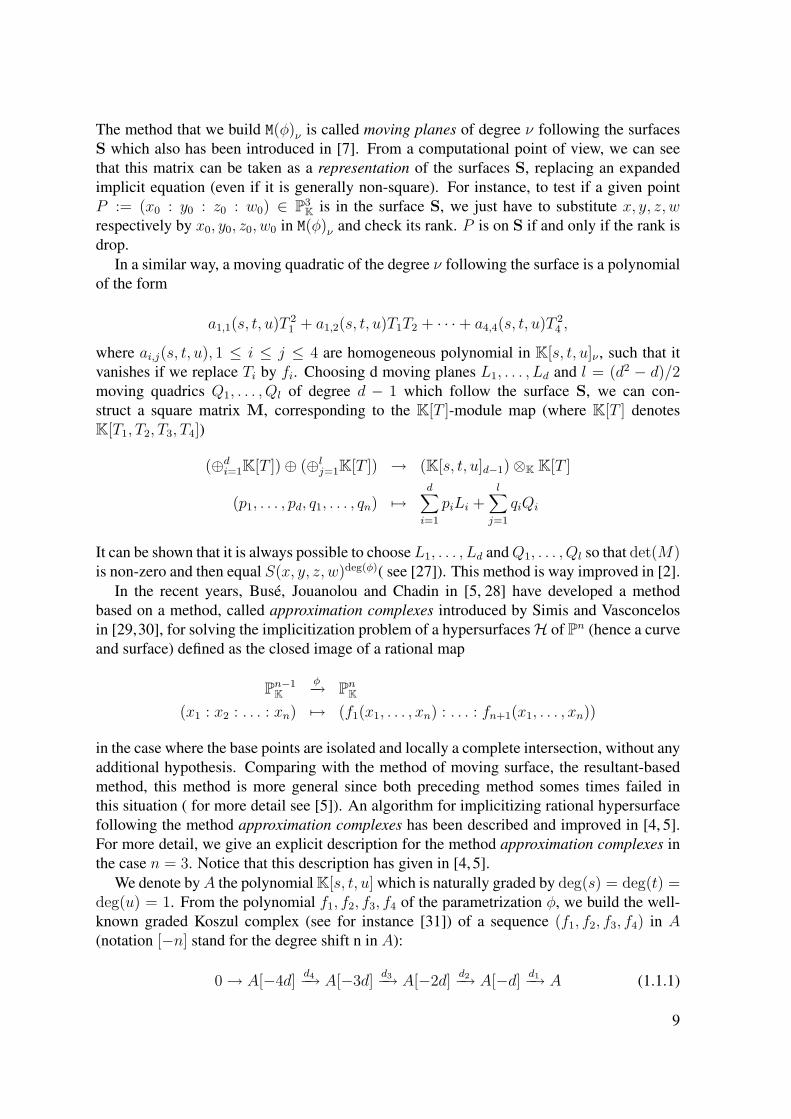
The method that we build M(φ)ν is called moving planes of degree ν following the surfacesS which also has been introduced in [7]. From a computational point of view, we can seethat this matrix can be taken as a representation of the surfaces S, replacing an expandedimplicit equation (even if it is generally non-square). For instance, to test if a given pointP := (x0 : y0 : z0 : w0) ∈ P3

K is in the surface S, we just have to substitute x, y, z, wrespectively by x0, y0, z0, w0 in M(φ)ν and check its rank. P is on S if and only if the rank isdrop.

In a similar way, a moving quadratic of the degree ν following the surface is a polynomialof the form

a1,1(s, t, u)T 21 + a1,2(s, t, u)T1T2 + · · ·+ a4,4(s, t, u)T 2

4 ,

where ai,j(s, t, u), 1 ≤ i ≤ j ≤ 4 are homogeneous polynomial in K[s, t, u]ν , such that itvanishes if we replace Ti by fi. Choosing d moving planes L1, . . . , Ld and l = (d2 − d)/2moving quadrics Q1, . . . , Ql of degree d − 1 which follow the surface S, we can con-struct a square matrix M, corresponding to the K[T ]-module map (where K[T ] denotesK[T1, T2, T3, T4])

(⊕di=1K[T ])⊕ (⊕lj=1K[T ]) → (K[s, t, u]d−1)⊗K K[T ]

(p1, . . . , pd, q1, . . . , qn) 7→d∑i=1

piLi +l∑

j=1qiQi

It can be shown that it is always possible to chooseL1, . . . , Ld andQ1, . . . , Ql so that det(M)is non-zero and then equal S(x, y, z, w)deg(φ)( see [27]). This method is way improved in [2].

In the recent years, Busé, Jouanolou and Chadin in [5, 28] have developed a methodbased on a method, called approximation complexes introduced by Simis and Vasconcelosin [29,30], for solving the implicitization problem of a hypersurfacesH of Pn (hence a curveand surface) defined as the closed image of a rational map

Pn−1K

φ−→ PnK(x1 : x2 : . . . : xn) 7→ (f1(x1, . . . , xn) : . . . : fn+1(x1, . . . , xn))

in the case where the base points are isolated and locally a complete intersection, without anyadditional hypothesis. Comparing with the method of moving surface, the resultant-basedmethod, this method is more general since both preceding method somes times failed inthis situation ( for more detail see [5]). An algorithm for implicitizing rational hypersurfacefollowing the method approximation complexes has been described and improved in [4, 5].For more detail, we give an explicit description for the method approximation complexes inthe case n = 3. Notice that this description has given in [4, 5].

We denote byA the polynomial K[s, t, u] which is naturally graded by deg(s) = deg(t) =deg(u) = 1. From the polynomial f1, f2, f3, f4 of the parametrization φ, we build the well-known graded Koszul complex (see for instance [31]) of a sequence (f1, f2, f3, f4) in A(notation [−n] stand for the degree shift n in A):

0→ A[−4d] d4−→ A[−3d] d3−→ A[−2d] d2−→ A[−d] d1−→ A (1.1.1)

9

where the differentials di(i = 1, 2, 3, 4) are given by

d4 =

−f4f3−f2f1

, d3 =

f3 f4 0 0−f2 0 f4 0f1 0 0 f40 −f2 −f3 00 f1 0 −f20 0 f1 f2

,

d2 =

−f2 −f3 0 −f4 0 0f1 0 −f2 0 −f4 00 f1 f2 0 0 −f40 0 f1 f2 f3

, d1 = (f1, f2, f3, f4).

Tensoring the complex (1.1.1) by A[x, y, z, w] over A, we obtain the complex denote by(K•(f1, f2, f3, f4), u•) which is of the form

0→ A[x, y, z, w][−4d] u4−→ A[x, y, z, w][−3d] u3−→ A[x, y, z, w][−2d] u2−→ A[x, y, z, w][−d]u1−→ A[x, y, z, w]

where the matrices of the differential di and ui are the same. Set deg(x) = deg(y) =deg(z) = deg(w) = 1, we build the bi-graded Koszul complex onA[x, y, z, w] of a sequence(x, y, z, w) denote by (K•(x, y, z, w), v•) which is of the form

0→ A[x, y, z, w][−4] v4−→ A[x, y, z, w][−3] v3−→ A[x, y, z, w][−2] v2−→ A[x, y, z, w][−1]v1−→ A[x, y, z, w]

and the matrices of its differentials are obtained from the matrices of the differentials (1.1.1)by replacing f1, f2, f3, f4 by x, y, z, w respectively. From the complex Koszul(K•(f1, f2, f3, f4), u•) and (K•(x, y, z, w), v•), we can build the complex Z• so-called ap-proximation complex by defining Zi := ker(di) ⊗A A[x, y, z, w] for i = 0, 1, 2, 3, 4 ( whered0 : A → 0). They are bi-graded A[x, y, z, w] - modules. For i = 1, 2, 3, we haveui vi+1 + vi ui+1 = 0, thus we obtain the bi-graded complex

(Z•, v•) : 0→ Z3(−3) v3−→ Z2(−2) v2−→ Z1(−1) v1−→ Z0 = A[x, y, z, w].

Remark 2. An element (g1, g2, g3, g4) ∈ Z1[ν] is a moving plane of degree ν following thesurface S. So the matrix of the surjective map

Z1[ν](−1) v1−→ Aν [x, y, z, w](g1, g2, g3, g4) 7→ xg1 + yg2 + zg3 + wg4

is exact the matrix M(φ)ν which we describe in the method moving surfaces.

Before giving the main properties of this collection of matrices, we need the following

Definition 3. A matrix M(φ) with entries in K[x, y, z, w] is said to be a representation of agiven homogeneous polynomial P ∈ K[x, y, z, w] if

10

i) M(φ) is generically full rank,

ii) the rank of M(φ) drops exactly on the surface of equation P = 0,

Recall that a point in P2K is called a base point of the parametrization φ if it is a common

root of the polynomials f1, . . . , f4. It is said to be locally a complete intersection if it can belocally generated by two equations, and said to be locally an almost complete intersection ifit can be locally generated by three equations.

Proposition 4 ( [4, 10]). For all integer ν ≥ 2(d− 1) we have:

• if the base points are local complete intersections then M(φ)ν represents Sdeg(φ),

• if the base points are almost local complete intersections then M(φ)ν represents

Sdeg(φ) ×∏

p∈V (f1,...,f4)⊂P2K

Lp(x, y, z, w)ep−dp

where Lp(x, y, z, w) are linear forms.

Remark 5. It is possible to improve the bound 2(d−1) by taking into account the geometry ofthe base points; we refer the reader to [4] for more details. For instance, if there exists at leastone common root to f1, . . . , f4 in P2 then the above proposition is true for all ν ≥ 2(d−1)−1.Also, mentioned that the linear forms Lp(x, . . . , w) can be determined by computations ofsyzygies in K[s, t, u]; see [10].

Although we are dealing with surfaces parametrized by the projective plane, it is importantto mention that the above results still hold for surfaces parametrized by the product of twoprojective lines, or more generally by a toric variety. We refer the interested reader to [1,9,32]for these extensions and also, a recent improvement of moving quadratics in [6]

1.2 Matrix-based implicit representations of rational alge-braic curves

In the previous part, we recalled an implicit representation of rational plane curve. In thispart, we introduce and study a new implicit representation of a rational curve in a projectivespace of arbitrary dimension. The results in this part have been published in [25]

1.2.1 The defining ideal of a rational curve and µ-basesLet f0, f1, . . . , fn be n homogeneous polynomials in K[s, t] of the same degree d ≥ 1 suchthat their greatest common divisor (GCD) is a non-zero constant in K. Consider the regularmap

P1K

φ−→ PnK(s : t) 7→ (f0(s, t) : f1(s, t) : · · · : fn(s, t)).

11

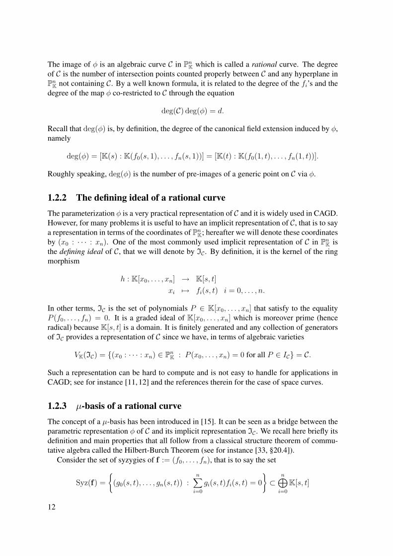
The image of φ is an algebraic curve C in PnK which is called a rational curve. The degreeof C is the number of intersection points counted properly between C and any hyperplane inPnK not containing C. By a well known formula, it is related to the degree of the fi’s and thedegree of the map φ co-restricted to C through the equation

deg(C) deg(φ) = d.

Recall that deg(φ) is, by definition, the degree of the canonical field extension induced by φ,namely

deg(φ) = [K(s) : K(f0(s, 1), . . . , fn(s, 1))] = [K(t) : K(f0(1, t), . . . , fn(1, t))].

Roughly speaking, deg(φ) is the number of pre-images of a generic point on C via φ.

1.2.2 The defining ideal of a rational curveThe parameterization φ is a very practical representation of C and it is widely used in CAGD.However, for many problems it is useful to have an implicit representation of C, that is to saya representation in terms of the coordinates of PnK; hereafter we will denote these coordinatesby (x0 : · · · : xn). One of the most commonly used implicit representation of C in PnK isthe defining ideal of C, that we will denote by IC . By definition, it is the kernel of the ringmorphism

h : K[x0, . . . , xn] → K[s, t]xi 7→ fi(s, t) i = 0, . . . , n.

In other terms, IC is the set of polynomials P ∈ K[x0, . . . , xn] that satisfy to the equalityP (f0, . . . , fn) = 0. It is a graded ideal of K[x0, . . . , xn] which is moreover prime (henceradical) because K[s, t] is a domain. It is finitely generated and any collection of generatorsof IC provides a representation of C since we have, in terms of algebraic varieties

VK(IC) = (x0 : · · · : xn) ∈ PnK : P (x0, . . . , xn) = 0 for all P ∈ IC = C.

Such a representation can be hard to compute and is not easy to handle for applications inCAGD; see for instance [11, 12] and the references therein for the case of space curves.

1.2.3 µ-basis of a rational curveThe concept of a µ-basis has been introduced in [15]. It can be seen as a bridge between theparametric representation φ of C and its implicit representation IC . We recall here briefly itsdefinition and main properties that all follow from a classical structure theorem of commu-tative algebra called the Hilbert-Burch Theorem (see for instance [33, §20.4]).

Consider the set of syzygies of f := (f0, . . . , fn), that is to say the set

Syz(f) =

(g0(s, t), . . . , gn(s, t)) :n∑i=0

gi(s, t)fi(s, t) = 0⊂

n⊕i=0

K[s, t]

12

It is known to be a free and graded K[s, t]-module of rank n. Moreover, there exists non-negative integers µ1, . . . , µn and n vectors of polynomials

(ui,0(s, t), ui,1(s, t), . . . , ui,n(s, t)) ∈ Syz(f) ⊂ K[s, t]n+1 (i = 1, . . . , n) (1.2.1)

such that

• for all i ∈ 1, . . . , n, j ∈ 0, . . . , n, ui,j(s, t) is a homogeneous polynomial inK[s, t] of degree µi ≥ 0,

• the n vectors in (1.2.1) form a K[s, t]-basis of Syz(f),

• ∑ni=1 µi = d,

• For all j ∈ 0, . . . , n, the determinant of the matrix obtained by deleting the column(ui,j)i=1,...,n from the matrix

M(s, t) :=

u1,0(s, t) u1,1(s, t) . . . u1,n(s, t)u2,0(s, t) u2,1(s, t) . . . u2,n(s, t). . . . . . . . . . . .

un,0(s, t) un,1(s, t) . . . un,n+1(s, t)

(1.2.2)

is equal to (−1)jc fj(s, t) ∈ K[s, t] where c ∈ K \ 0.

A collection of vectors as in (1.2.1) that satisfy the above properties is called a µ-basis of theparametrization φ. It is important to notice that a µ-basis is far from being unique, but thecollection of integers (µ1, µ2, . . . , µn) is unique if we order it. Therefore, in the sequel wewill always assume that a µ-basis is ordered so that 0 ≤ µ1 ≤ µ2 ≤ · · · ≤ µn. We refer theinterested reader to [13] for more details on the topic of µ-basis.

1.2.4 Projection of the graph of φHere is an important property of a µ-basis as a tool for the representation of the curve C.Recall that M(s, t) denotes the matrix (1.2.2) built from a µ-basis of φ.

Lemma 6. For any point (s0 : t0) ∈ P1K, the kernel of M(s0, t0) is K-generated by the

nonzero vector< f0(s0, t0), f1(s0, t0), . . . , fn(s0, t0) >

so that it has dimension exactly one. In particular, M(s0, t0) is full rank for any point(s0 : t0) ∈ P1

K.

Proof. Straightforward from the properties of a µ-basis and the classical Cramer’s rules.

For all i = 1, . . . , n set

ui(s, t, x0, x1, . . . , xn) =n∑j=0

ui,j(s, t)xj ∈ K[s, t, x0, . . . , xn]. (1.2.3)

13

An immediate consequence of Lemma 6 is that the algebraic variety W defined by the zerolocus of the µ-basis, i.e.

W := (s : t)× (x0 : · · · : xn) : u1 = u2 = · · · = un = 0 ⊂ P1K × PnK,

is nothing but the graph of the parameterization φ. Therefore, the canonical projection

π : P1K × PnK → PnK : (s : t)× (x0 : · · · : xn) 7→ (x0 : · · · : xn)

sends W on C; we have π(W ) = C (for more detail, see [34, Lecture 2]). But the situation isactually even nicer: this equality is not only true at the level of algebraic varieties, but alsoat the level of ideals. To be more precise we need some additional notation.

Define the polynomial ring A := K[x0, . . . , xn], so that K[s, t, x0, . . . , xn] = A[s, t], theideal I := (u1, . . . , un) of A[s, t] and consider its resultant ideal (also called the projectiveelimination ideal in [35, Chapter 8, §5]) A with respect to the ideal m = (s, t) of A[s, t]. Bydefinition, we have

A = P ∈ A such that ∃ ν ∈ N : (s, t)νP ⊂ I ⊂ A.

Proposition 7 ( [5, Corollary 3.8]). With the above notation, we have A = IC as ideals of A.

In the next section, we will take advantage of this proposition to produce a matrix-basedrepresentation of C. For that purpose, we will need a property that relates resultant idealswith certain annihilators. Define the quotient B := A[s, t]/I and recall that it inherits of astructure of graded ring from the canonical grading of C := A[s, t] and the homogeneousideal I: deg(s) = deg(t) = 1 and deg(a) = 0 for all a ∈ A. Set m := (s, t) ⊂ C and forany integer ν ∈ N consider

annA(Bν) = P ∈ A such that P.Bν = 0 ⊂ A.

Corollary 8. For all integer ν ≥ µn + µn−1 − 1 we have annA(Bν) = A = IC .

Proof. Since A = IC , we will explain why annA(Bν) = A for all ν ≥ µn + µn−1 − 1. First,define

H0m(B) :=

∞⋃k=0

(0 :B mk) = s ∈ B : ∃k ∈ N such that mks = 0.

It is a graded C-module and it is clear that A = H0m(B) ∩ A = H0

m(B)0. Moreover, for anyη ∈ N such that H0

m(B)η = 0, we have A = annA(Bη); see for instance [36, Proposition1.2].

Now, for any point (s0 : t0) ∈ P1K the variety V (u1(s0, t0), . . . , un(s0, t0)) is of codimen-

sion n in PnK by Lemma 6. Therefore, the polynomials u1, . . . , un form a regular sequencein A[s, t] outside V (m). It follows that we can apply the technics developed in [37, §2.10]and deduce that H0

m(B)ν = 0 for all ν ≥ µn + µn−1 − 1 (recall that we have assumed that0 ≤ µ1 ≤ · · · ≤ µn−1 ≤ µn).

The following aim is to produce a matrix-based representation of C which is geometri-cally faithful to the parameterization φ. In this order, we will exhibit ideals that are goodapproximations (in a sense that we will make precise hereafter) of the ideal IC . In view ofCorollary 8, certain Fitting ideals associated to a µ-basis of φ are natural candidates for thatpurpose.

14

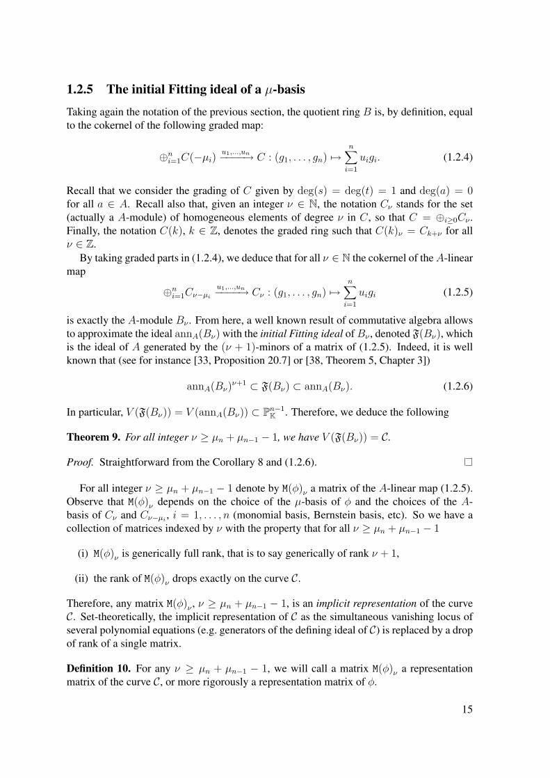
1.2.5 The initial Fitting ideal of a µ-basis

Taking again the notation of the previous section, the quotient ring B is, by definition, equalto the cokernel of the following graded map:

⊕ni=1C(−µi)u1,...,un−−−−→ C : (g1, . . . , gn) 7→

n∑i=1

uigi. (1.2.4)

Recall that we consider the grading of C given by deg(s) = deg(t) = 1 and deg(a) = 0for all a ∈ A. Recall also that, given an integer ν ∈ N, the notation Cν stands for the set(actually a A-module) of homogeneous elements of degree ν in C, so that C = ⊕i≥0Cν .Finally, the notation C(k), k ∈ Z, denotes the graded ring such that C(k)ν = Ck+ν for allν ∈ Z.

By taking graded parts in (1.2.4), we deduce that for all ν ∈ N the cokernel of theA-linearmap

⊕ni=1Cν−µiu1,...,un−−−−→ Cν : (g1, . . . , gn) 7→

n∑i=1

uigi (1.2.5)

is exactly the A-module Bν . From here, a well known result of commutative algebra allowsto approximate the ideal annA(Bν) with the initial Fitting ideal ofBν , denoted F(Bν), whichis the ideal of A generated by the (ν + 1)-minors of a matrix of (1.2.5). Indeed, it is wellknown that (see for instance [33, Proposition 20.7] or [38, Theorem 5, Chapter 3])

annA(Bν)ν+1 ⊂ F(Bν) ⊂ annA(Bν). (1.2.6)

In particular, V (F(Bν)) = V (annA(Bν)) ⊂ Pn−1K . Therefore, we deduce the following

Theorem 9. For all integer ν ≥ µn + µn−1 − 1, we have V (F(Bν)) = C.

Proof. Straightforward from the Corollary 8 and (1.2.6).

For all integer ν ≥ µn + µn−1 − 1 denote by M(φ)ν a matrix of the A-linear map (1.2.5).Observe that M(φ)ν depends on the choice of the µ-basis of φ and the choices of the A-basis of Cν and Cν−µi , i = 1, . . . , n (monomial basis, Bernstein basis, etc). So we have acollection of matrices indexed by ν with the property that for all ν ≥ µn + µn−1 − 1

(i) M(φ)ν is generically full rank, that is to say generically of rank ν + 1,

(ii) the rank of M(φ)ν drops exactly on the curve C.

Therefore, any matrix M(φ)ν , ν ≥ µn + µn−1 − 1, is an implicit representation of the curveC. Set-theoretically, the implicit representation of C as the simultaneous vanishing locus ofseveral polynomial equations (e.g. generators of the defining ideal of C) is replaced by a dropof rank of a single matrix.

Definition 10. For any ν ≥ µn + µn−1 − 1, we will call a matrix M(φ)ν a representationmatrix of the curve C, or more rigorously a representation matrix of φ.

15

Before moving on, let us justify the fact that a representation matrix really depends on φ,and not only on the curve C. Given an integer ν ≥ µn + µn−1 − 1, the ideal F(Bν) is notequal to the defining ideal IC of the rational curve C in general (see Example 12). However,F(Bν) is almost everywhere algebraically faithful to the parameterization φ in the followingsense.

Theorem 11. For all integer ν ≥ µn + µn−1− 1, we have the following equality of ideals inthe ring AIC which denotes the localization of A by the prime ideal IC:

F(Bν)IC = ICdeg(φ)AIC .

In other words, the ideals F(Bν) and ICdeg(φ) are equal at all points of C except a finite

number (possibly zero) of them.

Proof. Since IC = A = annA(Bν), Bν has a canonical structure of A/AA-module. More-over, since A is a prime ideal, we get that (Bν)A is a AA/AAA-vector space. Therefore, weonly need to prove that dimAA/AAA

(Bν)A = deg φ. This result is a consequence of the equal-ity (12) in the proof of Theorem 2.5 in [5] (see also the proof of Theorem 5.2 in loc. cit.).

Now, we have that (Bν)A ' (A/AA)deg(φ)A . Using classical properties of Fitting ideals

(see for instance [38, §3.1]) we deduce that

F(Bν)A ' F((A/AA)degφA ) = AdegφAA

as claimed.

This theorem shows that the ideal F(Bν) is equal to ICdeg(φ) plus a finite number (possi-

bly zero) of embedded isolated points on C. We illustrate this property with the followingexample.

Notice that in the rest of this chapter, when dealing with parameterized curves in P3K we

will often adopt the more commonly used notation (x, y, z, w) and (p, q, r) for the homoge-neous coordinates of P3

K and a µ-basis instead of the notation (x0, x1, x2, x3) and (u1, u2, u3).

Example 12. Let C be the rational space curve parameterized by

P1K

φ−→ P3K

(s : t) 7→ (s4 : s3t : s2t2 : t4).

A µ-basis of C is given by

p = −tx+ sy

q = −ty + sz,

r = −t2z + s2w.

We have µ1 = µ2 = 1, µ3 = 2 and hence µ3 + µ2 − 1 = 2. Therefore, we obtain thefollowing representation matrix of φ:

M(φ)2 =

y 0 z 0 w−x y −y z 00 −x 0 −y −z

.16

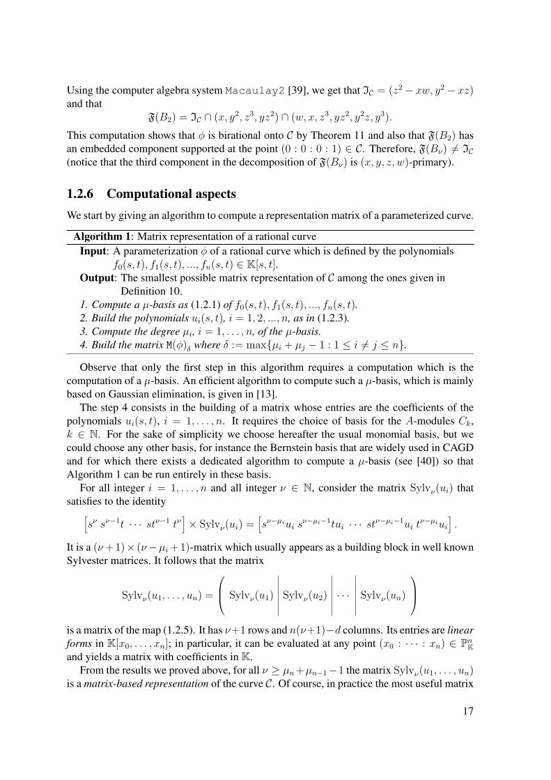
Using the computer algebra system Macaulay2 [39], we get that IC = (z2 − xw, y2 − xz)and that

F(B2) = IC ∩ (x, y2, z3, yz2) ∩ (w, x, z3, yz2, y2z, y3).This computation shows that φ is birational onto C by Theorem 11 and also that F(B2) hasan embedded component supported at the point (0 : 0 : 0 : 1) ∈ C. Therefore, F(Bν) 6= IC(notice that the third component in the decomposition of F(Bν) is (x, y, z, w)-primary).

1.2.6 Computational aspectsWe start by giving an algorithm to compute a representation matrix of a parameterized curve.

Algorithm 1: Matrix representation of a rational curveInput: A parameterization φ of a rational curve which is defined by the polynomials

f0(s, t), f1(s, t), ..., fn(s, t) ∈ K[s, t].Output: The smallest possible matrix representation of C among the ones given in

Definition 10.1. Compute a µ-basis as (1.2.1) of f0(s, t), f1(s, t), ..., fn(s, t).2. Build the polynomials ui(s, t), i = 1, 2, ..., n, as in (1.2.3).3. Compute the degree µi, i = 1, . . . , n, of the µ-basis.4. Build the matrix M(φ)δ where δ := maxµi + µj − 1 : 1 ≤ i 6= j ≤ n.

Observe that only the first step in this algorithm requires a computation which is thecomputation of a µ-basis. An efficient algorithm to compute such a µ-basis, which is mainlybased on Gaussian elimination, is given in [13].

The step 4 consists in the building of a matrix whose entries are the coefficients of thepolynomials ui(s, t), i = 1, . . . , n. It requires the choice of basis for the A-modules Ck,k ∈ N. For the sake of simplicity we choose hereafter the usual monomial basis, but wecould choose any other basis, for instance the Bernstein basis that are widely used in CAGDand for which there exists a dedicated algorithm to compute a µ-basis (see [40]) so thatAlgorithm 1 can be run entirely in these basis.

For all integer i = 1, . . . , n and all integer ν ∈ N, consider the matrix Sylvν(ui) thatsatisfies to the identity[

sν sν−1t · · · stν−1 tν]× Sylvν(ui) =

[sν−µiui s

ν−µi−1tui · · · stν−µi−1ui tν−µiui

].

It is a (ν+1)× (ν−µi+1)-matrix which usually appears as a building block in well knownSylvester matrices. It follows that the matrix

Sylvν(u1, . . . , un) =

Sylvν(u1) Sylvν(u2) · · · Sylvν(un)

is a matrix of the map (1.2.5). It has ν+1 rows and n(ν+1)−d columns. Its entries are linearforms in K[x0, . . . , xn]; in particular, it can be evaluated at any point (x0 : · · · : xn) ∈ PnKand yields a matrix with coefficients in K.

From the results we proved above, for all ν ≥ µn+µn−1−1 the matrix Sylvν(u1, . . . , un)is a matrix-based representation of the curve C. Of course, in practice the most useful matrix

17

is the smallest one, that is to say Sylvµn+µn−1−1(u1, . . . , un). We will illustrate in the nextchapter how one can take advantage of such a representation to perform important operationsof CAGD, as the curve/curve intersection problem or the detection of singular locus.

1.2.7 Rational curves contained in a planeMatrix representations of plane rational curves have been widely studied in the literature, sofor the sake of completeness we briefly mention it and show how the results presented in theprevious sections encapsulate it.

Assume that n = 2. Then C is a plane curve and IC is a principal ideal. It followsthat C is the zero locus of a single polynomial equation called an implicit equation (thisproperty never happens again if n > 2). A µ-basis is made of two elements u1 u2 suchthat µ2 + µ1 = d and it is well known that the Sylvester matrix of u1 and u2 is a squarematrix whose determinant is an implicit equation of C raised to the power deg(φ). Withthe notation of the previous sections, this Sylvester matrix is nothing but the representationmatrix M(φ)d−1. The particularity in the case n = 2 is that this matrix is square, which rarelyhappens (even in the case n = 2 since M(φ)ν is non square for ν ≥ d). Also, Theorem 11contains the fact the det(M(φ)d−1) is equal to an implicit equation of C raised to the powerdeg(φ). Here again, the particularity is that F(Bd−1) = Ideg(φ) since F(Bd−1) is a principalideal and hence cannot have embedded components.

Another interesting situation is the case of a curve C in Pn which is contained in a plane.By a linear change of coordinates, we can assume that the parameterization is of the form

P1K

φ−→ PnK(s : t) 7→ (f0(s, t) : f1(s, t) : f2(s, t) : 0 : · · · : 0)

so that C is included in the plane of equation x3 = x4 = . . . = xn = 0. Therefore a µ-basisis given by ui = xi, i = 3, . . . , n and u1, u2 is a µ-basis of the plane curve parameterized by

P1K

φ−→ P2K : (s : t) 7→ (f0(s, t) : f1(s, t) : f2(s, t)).

Then it is not hard to see that the representation matrix M(φ)d−1 (notice that µ1 +µ2 = d−1)is of the form

x3 0 xn 0M(φ)d−1

. . . · · · . . .

0 x3 0 xn

.

Let us end this paragraph with a last particular case: a line in P3 (we restrict ourselves toP3 for simplicity). Such a case occurs when µ1 = µ2 = 0. By a linear change of coordinates,we can suppose that u1 = x, u2 = y and u3 = p(s, t)z + q(s, t)w. Notice that necessarilyµ3 = d. In other words, the curve C is parameterized by

P1K

φ−→ P3K

(s : t) 7→ (0 : 0 : f2 : f3)(s, t).

18

We obtain the following matrix representation of φ where, notably, f2 and f3 does not appear(because C−1 = ∅):

M(φ)d−1 =

x 0 . . . 0 y 0 . . . 00 x . . . 0 0 y . . . 0...

... . . ....

...... . . .

...0 0 . . . x 0 0 . . . y

.

It is a d × 2d-matrix from we see easily find that F(Bd−1) = (x, y)d. It turns out that d isactually equal to deg(φ) from we get easily that F(Bν) = IC

deg(φ) in this case. This lastproperty follows from Luröth Theorem (see for instance [41]). Indeed, this theorem impliesthat there exists a commutative diagram

P1K

ϕ //

φ @@@

@@@@

P1K

ρ~~~~

~~~~

~

P3K

where

P1K

ρ−→ P3K

(x : y) 7→ (0 : 0 : x : y)(s, t),

P1K

ϕ−→ P1K

(t : s) 7→ (f2 : f3)(s, t),

and deg(φ) = deg(ρ) deg(ϕ), deg ρ = 1 and degϕ = d. Therefore, deg φ = d.

1.2.8 Matrix representations without µ-basesIn Section 1.2 we defined matrix representations of a rational curve. To build such a matrixit is necessary to first compute a µ-basis of the parameterization of the curve. There existefficient algorithms to compute µ-basis (see [13, 42]), but they all require the use of exactlinear algebra routines. Therefore, in order to make matrix representations accessible toany programming environment having linear algebra routines (but not necessarily exact), weprovide a new family of matrix representations that does not require symbolic computationsto be built. As we will see, the price to pay for this property is that the matrices we obtainare of bigger size than the ones obtained from a µ-basis.

Take again the notation of Section 1.2 and set

∆i,j =∣∣∣∣∣ fi(s, t) fj(s, t)

xi xj

∣∣∣∣∣for all 0 ≤ i < j ≤ n. The ∆i,j’s are the 2-minors of the matrix(

f0(s, t) f1(s, t) · · · fn−1(s, t) fn(s, t)x0 x1 · · · xn−1 xn

).

19

They are homogeneous polynomial in K[s, t;x0, . . . , xn]. More precisely they are linearforms in the homogeneous variables x0, . . . , xn and homogeneous polynomials of degree din the homogeneous variables s, t.

As in Section 1.2, set A = K[x0, . . . , xn], C = A[s, t] and consider the grading of C suchthat deg(s) = deg(t) = 1 and deg(a) = 0 for all a ∈ A. Now, consider the graded map

⊕0≤i<j≤n

C(−d) (...,∆i,j ,...)−−−−−−→ C : (· · · : gi,j : · · · ) 7→∑

0≤i<j≤ngi,j∆i,j (1.2.7)

and denote by B its cokernel.

Proposition 13. For all integer ν ≥ 2d− 1, we have Bν = Bν .

Proof. Consider the Koszul complex associated to the sequence (f0, . . . , fn) over the ringC. It is of the form

· · · →⊕

0≤i<j≤nC(−2d) ∂2−→

⊕0≤i<j≤n

C(−d) ∂1−→ C.

Observe then that the kernel of ∂1 is exactly the ideal generated by a µ-basis of φ and thatthe image of ∂2 is in correspondence with the syzygies of the fi’s that are of the form givenby the ∆i,j’s. Therefore, the difference between B and B is controlled by the first homologygroup H1 of this Koszul complex.

Now, by a classical property of Koszul complexes,H1 is annihilated by the ideal (f0, . . . , fn).Since φ is a regular map, we deduce that Bν = Bν for ν >> 0. Now, a classical spectralsequence (see for instance [37]) shows that we have a graded isomorphism, for all ν ∈ Z,

(H1)ν ' H2m(C(−3d))ν .

Therefore, we deduce that (H1)ν = 0 for all ν ≥ 3d− 1 and the result follows by noting thatH1 is embedded in the twisted graded ring C(−d).

By taking graded parts (1.2.7), for all integer ν ∈ N we obtain the A-linear map

⊕0≤i<j≤n

Cν−d(...,∆i,j ,...)−−−−−−→ Cν .

Denote by M(φ)ν a matrix of this map. Then, by Proposition 13, we have

Corollary 14. For all integer ν ≥ 2d− 1, the matrix M(φ)ν is a representation matrix of C.

The matrices M(φ)ν have exactly the same properties as the matrices M(φ)ν that are builtfrom a µ-basis. On the one hand, they do not require symbolic computations, but on the otherhand their sizes are much bigger. For instance, the matrix M(φ)2d−1 (the smallest one) is ofsize (2d)×

(n+1

2

)d whereas the matrix M(φ)d−1 (the smallest one) is of size d× (n− 1)d.

Example 15. Let C be the classical rational twisted cubic which is parameterized by

φ : P1K → P3

K : (s, t) 7→ (s3 : s2t : st2 : t3).

20

We have ∆i,j : 0 ≤ i < j ≤ 4 = s3y − s2tx, s3z − st2x, s3w − t3x, s2tz − st2y, s2tw −t3y, st2w − t3z. Choosing ν = 5 and the usual monomial basis, we obtain the followingmatrix representation of C:

M(φ)5 =

y 0 0 z 0 0 w 0 0 0 0 0 0 0 0 0 0 0−x y 0 0 z 0 0 w 0 z 0 0 w 0 0 0 0 00 −x y −x 0 z 0 0 w −y z 0 0 w 0 w 0 00 0 −x 0 −x 0 −x 0 0 0 −y z −y 0 w −z w 00 0 0 0 0 −x 0 −x 0 0 0 −y 0 −y 0 0 −z w0 0 0 0 0 0 0 0 −x 0 0 0 0 0 −y 0 0 −z

.

21

22

Chapter 2

Intersection problems with rationalcurves

In the first chapter, we introduced and studied the matrix-based implicit representations ofrational curves and rational surfaces. In this chapter, we will show how to use matrix-basedimplicit representations of rational curves and surfaces to solve some important problems inCAGD, namely the curve/curve and curve/surface intersection problems, the point-on-curveand inversion problems, the detection of singularities.

The idea of using matrix representations in CAGD to solve the intersection problemsis quite old. The novelty of our contribution is to enable non square matrices, extensionwhich is motivated by recent research in this topic. We show how to manipulate these repre-sentations by proposing a dedicated algorithm to address the curve/curve and curve/surfaceintersection problem by means of numerical linear algebra techniques.

The point-on-curve and inversion problems, the detection of singularities have been con-sidered recently in [13, 14, 18] with methods based on a set of equations that are built froma µ-basis of the parameterization. We will show in this chapter how the use of matrix-basedrepresentations allow to remove the limitations of the above methods in terms of the degreeof the curve and the multiplicities of singular points.

The results in this chapter have been published in two articles. The first one is a jointwork with Laurent Busé and Bernard Mourrain and have been published in [43]. The secondone is a joint work with Laurent Busé and have been published in [25]

Throughout this chapter, we assume that K is an algebraically closed field, typically thefield of complex numbers C.

2.1 Reduction of a univariate pencil of matrices

In this part, we will develop a numerical method to reduce generalized pencils of matrices.More precisely, in the theory of Kronecker forms (see for instance [44, Chapter 12]) we willreduce such a pencil to its regular part, avoiding this way the non square Kronecker blocks.

23

2.1.1 Linearization of a polynomial matrixWe begin with some notation.

Let A and B be two matrices of size m × n. We will call a generalized eigenvalue of Aand B a value in the set

λ(A,B) := t ∈ K : rank(A− tB) < minm,n

In the case m = n, the matrices A and B have n generalized eigenvalues if and only ifrank(B) = n. If rank(B) < n, then λ(A,B) can be finite, empty or infinite. Moreover, ifB is invertible then λ(A,B) = λ(AB−1, I) = λ(AB−1), which is the ordinary spectrum ofAB−1. The previous definition of generalized eigenvalues extends naturally to a polynomialmatrix M(t), where the entries are polynomials in t of any degree.

Suppose given an m× n-matrix M(t) = (ai,j(t)) with polynomial entries ai,j(t) ∈ K[t].It can be equivalently written as a polynomial in t with coefficients m × n-matrices withentries in K: if d = maxi,jdeg(ai,j(t)) then

M(t) = Mdtd +Md−1t

d−1 + . . .+M0

where Mi ∈ Km×n.

Definition 16. The generalized companion matricesA,B of the matrixM(t) are the matriceswith coefficients in K of size ((d− 1)m+ n)× dm that are given by

A =

0 I . . . . . . 00 0 I . . . 0...

......

......

0 0 . . . . . . IM t

0 M t1 . . . . . . M t

d−1

B =

I 0 . . . . . . 00 I 0 . . . 0...

......

......

0 0 . . . I 00 0 . . . . . . −M t

d

where I stands for the identity matrix and M t

i stands for the transpose of the matrix Mi.

We have the following interesting property that follows from a straightforward computa-tion.

Proposition 17. With the above notation, for all t ∈ K and all vector v ∈ Km we have

M t(t)v = 0⇔ (A− tB)

vtv...

td−1v

= 0.

24

Because rankM(t) = rankM t(t), from now on we will assume that M(t) is an m× n-matrix such that m ≤ n. Therefore, rankM(t) drops if and only if rankM(t) < m.

Theorem 18. With the above assumptions, the following equivalence holds:

rankM(t) < m⇔ rank(A− tB) < dm.

Proof. Because rankM(t) = rankM t(t), we have that rankM t(t) < m. Thus, thereexists a column vector v 6= 0 such that M t(t)v = 0. Then, by Proposition 17 equation(A− tB)x = 0 has a nonzero root. That means exactly that rank(A− tB) < dm.

Now, if rank(A − tB) < dm, then equation (A − tB)x = 0 have a root x 6= 0 and by astraightforward computation it is of the form

x =

vtv...

td−1v

.

Since x 6= 0 and by Proposition 17, we have v 6= 0 and v is a root of equation M t(t)v = 0.Thus, rankM t(t) < m and it follows that rankM(t) < m.

By Theorem 18, we transformed the computation of generalized eigenvalues of the matrixpolynomial M(t) (that is to say the roots of the gcd of the maximal minors of M(t)) into thecomputation of generalized eigenvalues of a pencil of matrices A− tB. If the matrices A,Bwere two square matrices, then we could easily compute their generalized eigenvalues bythe QZ-algorithm [45]. Therefore, our next task is to reduce the pencil A− tB into a squarepencil that keeps the information we are interested in.

Before moving on, we recall what is the Smith form of M(t) for future use. Assume thatrankM(t) = r, it exists two regular polynomial matrices with nonzero determinant in K,say P (t) and Q(t), such that

D(t) = P (t)M(t)Q(t) =

ar(t) 0 . . . . . . . . . 00 ar−1(t) 0 . . . . . . 0...

......

......

...0 . . . . . . a1(t) . . . 00 0 . . . . . . . . . 0

where ai(t)’s are monic polynomials and ai(t) divides ai−1(t). This form is unique and iscalled the Smith form of M(t) (see for instance [46, Chapter 6]). Notice that by performingunimodular row and column transformations on the matrix A− tB, we can find that A− tBhas the Smith form (see for instance [47, 48] for more details)

U(t)(A− tB)V (t) = diagIm, ..., Im, D(t)

where D(t) is the Smith form of M t(t). Thus, Theorem 18 can be recovered from thisproperty.

25

2.1.2 The Kronecker form of a non square pencil of matricesHereafter, we recall some known properties of the Kronecker form of pencils of matrices.

Definition 19. Let Lk(t),Ωk(t) be the two matrices of size k×(k+1) and k×k respectively,defined by

Lk(t) =

1 t 0 . . . 00 1 t . . . 0...

......

......

0 . . . 1 t 00 0 . . . 1 t

,

Ωk(t) =

1 t 0 . . . 00 1 t . . . 0...

......

......

0 . . . . . . 1 t0 0 . . . 0 1

.

We are going to use the following theorem, which gives what is called the Kroneckercanonical form of a pencil of matrices (see for instance [44, p. 31-34]).

Theorem 20. For any couple constant matrices A, B of size p × q, there exist constantinvertible matrices P and Q such that the pencil P (A− tB)Q is of the block-diagonal form

diagLi1 , ..., Lis , Ltj1 , ..., Ltju ,Ωk1 , ...,Ωkv , A

′ − tB′

whereA′, B′ are square matrices andB′ is invertible. The dimension i1, ..., is, j1, ..., ju, k1, .., kvand the determinant of A′ − tB′ (up to a scalar) are independent of the representation.

This theorem can be implemented as follows:

Proposition 21. For any couple of matrices C0, C1 of size p× q, there exist unitary matricesU and V such that the pencil

U(C0 − tC1)V = C0 − tC1

is of the form

C(t) =

Cl(t) C1,2(t) C1,3(t)0 Cr(t) C2,2(t)0 0 Creg(t)

where

• Cl(t) = Cl,0−tCl,1 has only blocks of the form Lk(t),Ωk(t) in its Kronecker canonicalform,

• Cr(t) = Cr,0 − tCr,1 has only blocks of the form Ltk(t),

• Creg(t) = Creg,0 − tCreg,1 is a square regular pencil.

26

It is interesting to notice that the above decomposition can be computed within O(p2q)arithmetic operations. We refer the reader to [49, 50] for a proof, as well as for an analysisof the stability of this decomposition.

Following the ideas developed in [49,50] and the reduction methods exploited in [51,52],we now describe an algorithm that allows to remove the Kronecker blocks Lk, Ltk and Ωk ofthe pencil of matrices A− tB in order to extract the regular pencil A′ − tB′.

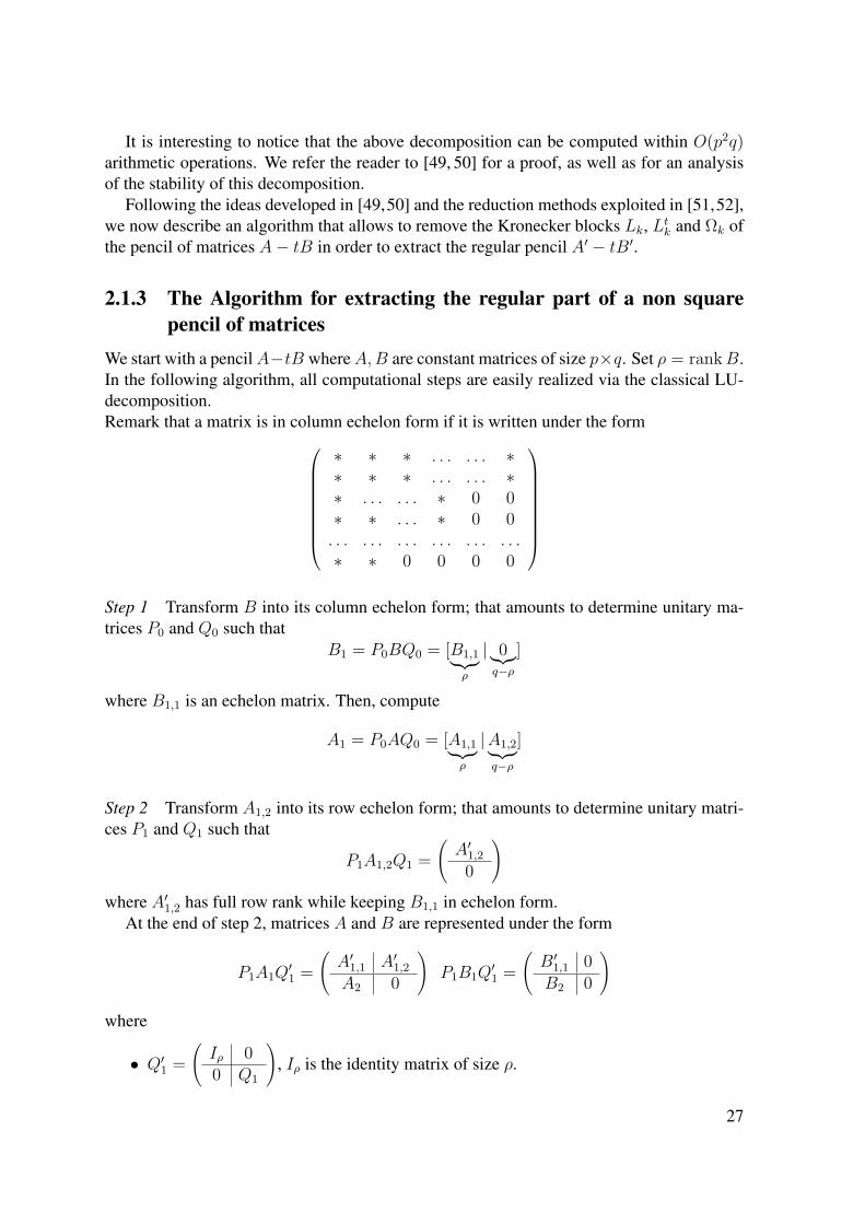
2.1.3 The Algorithm for extracting the regular part of a non squarepencil of matrices

We start with a pencilA−tB whereA,B are constant matrices of size p×q. Set ρ = rankB.In the following algorithm, all computational steps are easily realized via the classical LU-decomposition.Remark that a matrix is in column echelon form if it is written under the form

∗ ∗ ∗ . . . . . . ∗∗ ∗ ∗ . . . . . . ∗∗ . . . . . . ∗ 0 0∗ ∗ . . . ∗ 0 0. . . . . . . . . . . . . . . . . .∗ ∗ 0 0 0 0

Step 1 Transform B into its column echelon form; that amounts to determine unitary ma-trices P0 and Q0 such that

B1 = P0BQ0 = [B1,1︸︷︷︸ρ

| 0︸︷︷︸q−ρ

]

where B1,1 is an echelon matrix. Then, compute

A1 = P0AQ0 = [A1,1︸︷︷︸ρ

|A1,2︸︷︷︸q−ρ

]

Step 2 Transform A1,2 into its row echelon form; that amounts to determine unitary matri-ces P1 and Q1 such that

P1A1,2Q1 =(A′1,20

)where A′1,2 has full row rank while keeping B1,1 in echelon form.

At the end of step 2, matrices A and B are represented under the form

P1A1Q′1 =

(A′1,1 A′1,2A2 0

)P1B1Q

′1 =

(B′1,1 0B2 0

)

where

• Q′1 =(Iρ 00 Q1

), Iρ is the identity matrix of size ρ.

27

• A′1,2 has full row rank,

•(B′1,1B2

)has full column rank,

•(B′1,1B2

)and B2 are in echelon form.

After steps 1 and 2, we obtain a new pencil of matrices, namely A2 − tB2.

Step 3 Starting from j = 2, repeat the above steps 1 and 2 for the pencil Aj − tBj until thepj × qj matrix Bj has full column rank, that is to say until rankBj = qj .

IfBj is not a square matrix, then we repeat the above procedure with the transposed pencilAtj − tBt

j .At last, we obtain the regular pencil A′ − tB′ where A′, B′ are two square matrices and

B′ is invertible.

2.2 Curve/surface intersectionSuppose given an algebraic surface S represented by a homogeneous and irreducible implicitequation S(x, y, z, w) = 0 in P3

K and a rational space curve C represented by a parameteri-zation

Ψ : P1K → P3

K : (s : t) 7→ (x(s, t) : y(s, t) : z(s, t) : w(s, t))where x(s, t), y(s, t), z(s, t), w(s, t) are homogeneous polynomials of the same degree andwithout common factor in K[s, t].

A standard problem in non linear computational geometry is to determine the set C ∩S ⊂ P3

K, especially when it is finite. One way to proceed, is to compute the roots of thehomogeneous polynomial

S(x(s, t), y(s, t), z(s, t), w(s, t)) (2.2.1)

because they are in correspondence with C ∩ S through the regular map Ψ. Observe that(2.2.1) is identically zero if and only if C ∩ S is infinite, equivalently C ⊂ S (for C isirreducible).

If S is a rational surface represented by a parameterization, then several authors (seefor instance [8] and the references therein) used some square matrix representations, mostof the time obtained from a particular resultant matrix, of S in order to compute the setC ∩ S by means of eigencomputations. As we have already mentioned, such square matrixrepresentations exist only under some restrictive conditions. Hereafter, we would like togeneralize this approach for non square matrix representation that can be obtained for amuch larger class of rational surfaces and are very easy to compute.

So, assume that M(x, y, z, w) is a matrix representation of the surface S, meaning a rep-resentation of the polynomial S(x, y, z, w). By replacing the variables x, y, z, w by the ho-mogeneous polynomials x(s, t), y(s, t), z(s, t), w(s, t) respectively, we get the matrix

M(s, t) = M(x(s, t), y(s, t), z(s, t), w(s, t))

28

and we have the following easy property:

Lemma 22. With the above notation, for all point (s0 : t0) ∈ P1K the rank of the matrix

M(s0, t0) drops if and only if the point (x(s0, t0) : y(s0, t0) : z(s0, t0) : w(s0, t0)) belongs tothe intersection locus C ∩ S.

It follows that points in C ∩ S associated to points (s : t) such that s 6= 0, are in corre-spondence with the set of values t ∈ K such that M(1, t) drops of rank strictly less than itsrow and column dimensions i.e. the set of generalized eigenvalues of M(1, t).

We are now ready to give our algorithm for solving the curve/surface intersection prob-lem:

Algorithm 2: Matrix intersection algorithmInput: A matrix representation of a surface S and a parametrization of a rational space

curve C.Output: The intersection points of S and C.1. Compute the matrix representation M(t).2. Compute the generalized companion matrices A and B of M(t).3. Compute the companion regular matrices A′ and B′.4. Compute the eigenvalues of (A′, B′).5. For each eigenvalue t0, the point P (x(t0) : y(t0) : z(t0) : w(t0)) is one of the intersectionpoints.

2.2.1 The multiplicity of an intersection point

In this section, we analyze more precisely the multiplicity of an intersection point and showits correlation with the corresponding eigenvalue multiplicity for the polynomial matrixM(1, t). We assume hereafter, without loss of generality, that the intersection point is atfinite distance.

Let (∆i(x, y, z, w))i=1,...,N be the set of all maximal minors of a representation matrixM(x, y, z, w) of S. By definition, for all i = 1, . . . , N there exists a polynomialHi(x, y, z, w)such that ∆i = HiS and gcd(H1, . . . , HN) is a nonzero constant in K[x, y, z, w]. Therefore,the zero locus of the polynomialsH1, . . . , HN , S is an algebraic variety W which is includedin S and which has projective dimension at most one.

Hereafter, we will often abbreviate x(1, t) by x(t) to not overload the text, and will dosimilarly for the other polynomials y, z, w. Let P = (x(t0) : y(t0) : z(t0) : w(t0)) be a pointon the parameterized curve C. The intersection multiplicity of S and C at P can be definedas

IP =∑

ti such that Ψ(ti)=PdimK

(K[t]

S(x(t), y(t), z(t), w(t))

)(t−ti)

assuming w.l.o.g. that Ψ is birational onto C (by Luröth Theorem [41]) and that all the pre-images of P are at finite distance (that can be achieved by a linear change of coordinates).

29

Of course, if P ∈ C ∩ S then IP > 0 and IP = 0 otherwise. Also, if P is non singular pointon C (recall that the set of singular points on C is finite) then

IP = dimK

(K[t]

S(x(t), y(t), z(t), w(t))

)(t−t0)

Now, denote bymλ the multiplicity of λ as a generalized eigenvalue of the matrixM(t) =M(x(t), . . . , w(t)). From the above considerations, it follows that the intersection multiplic-ity of a point P = (x(t0) : y(t0) : z(t0) : w(t0)) ∈ C ∩ S such that P /∈ W is exactly thesum of the multiplicity of the corresponding eigenvalues:

IP =∑

ti such that Ψ(ti)=Pmti

As already noticed, if P is moreover smooth on C, then IP = mt0 . Now, if P ∈W∩C∩S,then

IP <∑

ti such that Ψ(ti)=Pmti

due to the existence of embedded components (determined by the polynomials Hi’s) thatcome from the matrix representation of S.

Notice that if the surface S is given by a parameterization which is not birational onto itsimage, then the matrix representations that we describe in the first chapter actually representthe implicit equation of S up to a certain power, say β. In such case, one has similar resultsregarding the multiplicities of intersection points:

βIP =∑

ti such that Ψ(ti)=Pmti

If P is smooth on C, then βIP = mt0 and

βIP <∑

ti such that Ψ(ti)=Pmti

if P ∈W ∩C ∩ S.Now, we are going to relate this multiplicity with the multiplicity of the corresponding

eigenvalue of the pencil of matrices built in Section 2.1.3.With the notations of Section 2.1.3, we have:

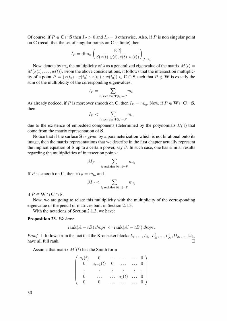
Proposition 23. We have

rank(A− tB) drops ⇔ rank(A′ − tB′) drops.

Proof. It follows from the fact that the Kronecker blocksLi1 , ..., Lis , Ltj1 , ..., L

tju , Ωk1 , ...,Ωkv

have all full rank.

Assume that matrix M t(t) has the Smith form

ar(t) 0 . . . . . . . . . 00 ar−1(t) 0 . . . . . . 0...

......

......

...0 . . . . . . a1(t) . . . 00 0 . . . . . . . . . 0

30

We set

U(t) =

as(t) 0 . . . . . . 0

0 as−1(t) 0 . . . 0...

......

......

0 . . . . . . 0 a1(t)

Notice that U(t) is a square matrix where a1(t), . . . , as(t) are monic non constant polynomi-als.

Proposition 24. The Smith form of the regular pencil A′ − tB′ is of the form Ik, U(t).Proof. We know that the matrix A− tB has the Kronecker form

diagLi1 , ..., Lis , Ltj1 , ..., Ltju ,Ωk1 , ...,Ωkv , A

′ − tB′

and the Smith form (see for instance [47])

diagIm, ..., Im, D(t).

On the other hand, we easily see that the Kronecker blocks Lk(t), Ltk(t) and Ωk(t) haverespectively the Smith form

1 0 0 . . . 00 1 0 . . . 0...

......

......

0 . . . 1 0 00 0 . . . 1 0

,

1 0 0 . . . 00 1 0 . . . 0...

......

......

0 . . . . . . 0 10 0 . . . 0 0

,

1 0 0 . . . 00 1 0 . . . 0...

......

......

0 . . . . . . 1 00 0 . . . 0 1

.

Therefore, the regular pencil A′ − tB′ has the Smith form Ik, U(t).Theorem 25. If A′ − tB′ denotes the regular part of a pencil associated to a representationmatrix of the intersection between a surface S and a rational parametric curve C then theintersection multiplicity of S and C at a point P = (x(t0) : y(t0) : z(t0) : w(t0)) is equal tothe multiplicity of the eigenvalues (A′, B′) at t0, except in few cases where this multiplicityis strictly bigger.

Proof. BecauseM(t) is them×n-matrix (m ≤ n) representation of the intersection betweenS and C, M t(t) has the Smith form

am(t) 0 . . . . . . . . . 00 am−1(t) 0 . . . . . . 0...

......

......

...0 . . . . . . . . . . . . a1(t)...

......

......

...0 0 . . . . . . . . . 0

,

31

Let F (t) = am(t)am−1(t)...a1(t). By Proposition 24, we have F (t) = c det(A′ − tB′),where c is a nonzero constant.The multiplicity of the eigenvalue of (A′, B′) at t0 is equalto the multiplicity of the root t0 of F (t) and therefore to the multiplicity of S and C at apoint P = (x(t0) : y(t0) : z(t0) : w(t0)), expect in few cases that are described in Section2.2.1.

Remark 26. In the statement of this theorem, the few cases where the multiplicity as an inter-section point is strictly less than the multiplicity of the corresponding generalized eigenvalueare exactly the cases where the curve cut out the surface on W, taking again notation ofSection 2.2.1. It turns out that W is a closed variety in S and hence the measure of W in Sis null. Therefore, these cases have a null probability to happen if the surface and the curveare supposed arbitrary.

We have implemented our curve/surface intersection algorithm, as well as the matrixrepresentations given in the first chapter, in the software MAPLE or the software MATH-EMAGIX. Hereafter, we provide some examples to illustrate it.

Example 27. Let S be the rational surface which is parametrized by

φ : P2 → P3 : (s : t : u) 7→ (f1 : f2 : f3 : f4)

wheref1 = s3 + t2u, f2 = s2t+ t2u, f3 = s3 + t3, f4 = s2u+ t2u.

We want to compute the intersection of S and the rational curve C, often called the twistedcubic, given by the parameterization

x(t) = 1, y(t) = t, z(t) = t2, w(t) = t3.

First, on computes a matrix representation of S:

0 0 0 w − y 0 0 z − xw 0 0 x w − y 0 0

x− y − z 0 0 −z 0 w − y 00 w 0 0 x 0 −y0 x− y − z w 0 −z x y + z − x0 0 x− y − z 0 0 −z 0

A point P at finite distance belongs to the intersection locus of S and C if and only if

P = (1 : t : t2 : t3) and t is one of the generalized eigenvalues of the following matrix M(t)given by

0 0 0 t3 − t 0 0 t2 − 1t3 0 0 1 t3 − t 0 0

1− t− t2 0 0 −t2 0 t3 − t 00 t3 0 0 1 0 −t0 1− t− t2 −t3 0 −t2 1 t2 + t− 10 0 1− t− t2 0 0 −t2 0

32

We have M(t) = M3t3 +M2t

2 +M1t+M0 where M0,M1,M2,M3 are respectively

0 0 0 0 0 0 −10 0 0 1 0 0 01 0 0 0 0 0 00 0 0 0 1 0 00 1 0 0 0 1 −10 0 1 0 0 0 0

,

0 0 0 −1 0 0 00 0 0 0 −1 0 0−1 0 0 0 0 −1 00 0 0 0 0 0 −10 −1 0 0 0 0 10 0 −1 0 0 0 0

,

0 0 0 0 0 0 10 0 0 0 0 0 0−1 0 0 −1 0 0 00 0 0 0 0 0 00 −1 0 0 −1 0 10 0 −1 0 0 −1 0

,

0 0 0 1 0 0 01 0 0 0 1 0 00 0 0 0 0 1 00 1 0 0 0 0 00 0 1 0 0 0 00 0 0 0 0 0 0

.

and the generalized companion matrices of M(t) are

A =

0 I 00 0 IM t

0 M t1 M t

2

, B =

I 0 00 I 00 0 −M t

3

Now, applying the algorithm given in Section 2.1.3, we find that the regular part of the pencilA− tB is the pencil A′ − tB′ where A′ is given by

0 0 0 0 0 0 0 0 0 0 0 1 00 1 0 0 1 0 1 0 0 0 0 −1 10 0 0 0 0 0 0 1 0 0 0 −1 01 0 0 0 0 0 0 0 0 0 0 0 00 0 0 0 0 0 0 0 −1 0 0 0 −10 2 0 0 2 0 2 0 −1 −1 −2 −2 10 −1 0 0 −1 0 −1 0 2 0 1 1 00 1 0 0 1 0 1 0 −1 −1 −1 −1 00 1 0 −1 1 0 1 0 0 0 −1 −1 10 0 0 0 0 −1 0 0 1 0 0 0 00 1 0 0 1 0 0 0 −1 0 −1 −1 00 1 −1 0 1 0 1 0 −1 −1 −1 −1 00 −1 0 0 −2 0 −1 0 0 0 1 2 −1

,

33

and B′ is the identity matrix. Then, we compute the following eigenvalues: t1 = 1 withmultiplicity 3, t2 = −1 with multiplicity 3 and the roots of the equation Z7 + 3Z6 − Z5 −Z3 + Z2 − 2Z + 1 = 0.

Example 28. Let S be the sphere that we suppose given as the image of the parametrization

φ : P2 → P3 : (s : t : u) 7→ (f1 : f2 : f3 : f4)

wheref1 = s2 + t2 + u2, f2 = 2su, f3 = 2st, f4 = s2 − t2 − u2

Let C be the twisted cubic which is parametrized by

x(t) = 1, y(t) = t, z(t) = t2, w(t) = t3.

The computation of a matrix representation of the sphere S gives −y 0 z x+ w0 −y −x+ w −zz x+ w y 0

.Now, a point P belongs to the intersection of S and C if and only if P = (1 : t : t2 : t3)

and t is one of the generalized eigenvalues of the matrix

M(t) =

−t 0 t2 1 + t3

0 −t −1 + t3 −t2t2 1 + t3 t 0

.As before, we easily compute the eigenvalues and find:

t1 = 0.7373527056, t2 = −0.7373527056,

t3 = 0.5405361044 + 1.031515287i, t4 = −0.5405361044− 1.031515287i,

t5 = 0.5405361044− 1.031515287i, t6 = −0.5405361044 + 1.031515287i.

All these eigenvalues have multiplicity 1. They all correspond to one intersection pointbetween S and C which has multiplicity 1. By Bezout Theorem, we find here all the inter-section points between these two algebraic varieties (all of them are at finite distance).

Example 29. As the previous example, let S be the sphere given be the same parametrizationand matrix representation. Here, we want to intersect S with a simple curve C: the lineparametrized by

x(t) = 1, y(t) = 0, z(t) = 0, w(t) = t.

In this case we have

M(t) =

0 0 0 t+ 10 0 −1 + t 00 1 + t 0 0

.34

Figure 2.1: Intersection of the sphere and the twisted cubic, the axis Oz

We proceed as in the previous example and now find two eigenvalues: t1 = −1 with mul-tiplicity 2 and t2 = +1 with multiplicity 1. They correspond to the intersection pointsP1(1 : 0 : 0 : −1) and P2(1 : 0 : 0 : 1) respectively.

It is interesting to notice that in this case the multiplicity of the eigenvalue t1, which is 2,is not equal to the multiplicity of the intersection point P1, which is 1. This is due to the factthat the matrix representation of S introduces an embedded point, namely P1 itself, on thesphere. Indeed, the four maximal minors of the matrix representation of S are given by

−y(−y2 + x2 − w2 − z2), z(−y2 + x2 − w2 − z2),

(x+ w)(−y2 + x2 − w2 − z2), 0.Therefore, the zero locus defined by the equations x + w, y, z,−y2 + x2 − w2 − z2, whichis nothing but the point P1, is an embedded component on the sphere.

2.3 Curve/curve intersectionSuppose given two rational curves, say C1 parameterized by

P1 φ1−→ Pn : (s : t) 7→ (f0 : · · · : fn)(s, t) (2.3.1)

and C2 parameterized by the regular map

P1 φ2−→ Pn : (s : t) 7→ (g0 : · · · : gn)(s, t). (2.3.2)

Let M(φ)ν(φ1) be a representation matrix of C1 for a suitable integer ν, as described in Section1.2. The substitution in M(φ)ν(φ1) of the variables x, y, z, w by the homogeneous parameter-ization of C2 yields the matrix

M(φ)ν(φ1)(s, t) := M(φ)ν(φ1)(g0(s, t), . . . , gn(s, t))

As a consequence of the properties of a representation matrix, we have the following easyproperty.

35

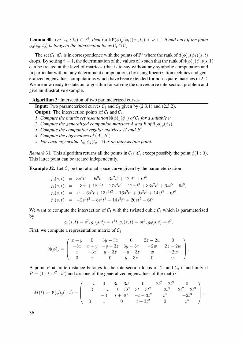
Lemma 30. Let (s0 : t0) ∈ P1, then rank M(φ)ν(φ1)(s0, t0) < ν + 1 if and only if the pointφ2(s0, t0) belongs to the intersection locus C1 ∩ C2.

The set C1∩C2 is in correspondence with the points of P1 where the rank of M(φ)ν(φ1)(s, t)drops. By setting t = 1, the determination of the values of s such that the rank of M(φ)ν(φ1)(s, 1)can be treated at the level of matrices (that is to say without any symbolic computation andin particular without any determinant computations) by using linearization technics and gen-eralized eigenvalues computations which have been extended for non-square matrices in 2.2.We are now ready to state our algorithm for solving the curve/curve intersection problem andgive an illustrative example.

Algorithm 3: Intersection of two parameterized curvesInput: Two parameterized curves C1 and C2 given by (2.3.1) and (2.3.2).Output: The intersection points of C1 and C2.1. Compute the matrix representation M(φ)ν(φ1) of C1 for a suitable ν.2. Compute the generalized companion matrices A and B of M(φ)ν(φ1).3. Compute the companion regular matrices A′ and B′.4. Compute the eigenvalues of (A′, B′).5. For each eigenvalue t0, φ2(t0 : 1) is an intersection point.

Remark 31. This algorithm returns all the points in C1∩C2 except possibly the point φ(1 : 0).This latter point can be treated independently.

Example 32. Let C1 be the rational space curve given by the parameterization

f0(s, t) = 3s4t2 − 9s3t3 − 3s2t4 + 12st5 + 6t6,f1(s, t) = −3s6 + 18s5t− 27s4t2 − 12s3t3 + 33s2t4 + 6st5 − 6t6,f2(s, t) = s6 − 6s5t+ 13s4t2 − 16s3t3 + 9s2t4 + 14st5 − 6t6,f3(s, t) = −2s4t2 + 8s3t3 − 14s2t4 + 20st5 − 6t6.

We want to compute the intersection of C1 with the twisted cubic C2 which is parameterizedby

g0(s, t) = s3, g1(s, t) = s2t, g2(s, t) = st2, g3(s, t) = t3.

First, we compute a representation matrix of C1:

M(φ)3 =

x+ y 0 3y − 3z 0 2z − 2w 0−3x x+ y −y − 3z 3y − 3z −2w 2z − 2wx −3x y + 3z −y − 3z w −2w0 x 0 y + 3z 0 w

.A point P at finite distance belongs to the intersection locus of C1 and C2 if and only ifP = (1 : t : t2 : t3) and t is one of the generalized eigenvalues of the matrix

M(t) := M(φ)3(1, t) =

1 + t 0 3t− 3t2 0 2t2 − 2t3 0−3 1 + t −t− 3t2 3t− 3t2 −2t3 2t2 − 2t31 −3 t+ 3t2 −t− 3t2 t3 −2t30 1 0 t+ 3t2 0 t3

,

36

We have M(t) = M3t3 + M2t

2 + M1t + M0 and the generalized companion matrices ofM(t) are

A =

0 I 00 0 IM t

0 M t1 M t

2

, B =

I 0 00 I 00 0 −M t

3

Applying Algorithm 3, we find that the regular part of the pencilA−tB is the pencilA′−tB′where A′, B′ are given by

A′ =(

0 00 0

), B′ =

(1 00 1

).

Therefore, the computation yields a single eigenvalues t = 0, and thus C1 intersect C2 at theonly point P = (1 : 0 : 0 : 0).

We can also determine the parameter(s) corresponding to P through the parameterizationφ1 of C1. For that purpose, we first evaluate the rank of the matrix M(φ)3(P ). It is equal to 2.Therefore, P is a singular point of multiplicity 2. It follows that it is not possible to apply theinversion method given in Section 2.3.2, but rather the method for computing the singularpoints of C1 given in Section 2.4. We get that P is obtained through the two parameters(1 : 1

2(3 +√

5)) and (1 : 12(3−

√5)) via φ1.

Example 33. We have implemented Algorithm 3 in the software Maple. The correspond-ing files are available at http://www-sop.inria.fr/members/Luu.Ba_Thang/.Consider the two curves parameterized, in affine coordinate, by

f0(t) = −33 + 1152 t− 49

2 t2 + t4,

f1(t) = −36 + 61 t− 25 t2 + t4,

f2(t) = −8 + 272 t− 13/2 t2 + t3,

f3(t) = 1.

and

g0(t) = −3 + 17/2 t− 11/2 t2 + t3,

g1(t) = −6 + 12 t− 6 t2 + t3,

g2(t) = −38 + 1252 t− 51

2 t2 + t4,

g3(t) = 1.

Running our algorithm, we find 4 values of the parameter t that corresponds to an in-tersection point, namely t = −5, 1, 2, 3. These four intersection points, of coordinates(1, 1, 0), (0, 2, 1), (0, 3, 1) and (−308,−341,−363) can be visualized in the following pic-tures.

37

2.3.1 Line intersection of two ruled surfacesThe aim of this section is to show that curves in a projective space of higher dimension than3 can be useful for applications in CAGD. Hereafter, we consider the problem of computingline intersections between two ruled surfaces. As we will see, this can be done by computingthe intersection of two rational curves in a P5, a problem that can be solved by using thetechnics we have presented in the previous section.

It is worth mentioning that the computation of the intersection lines between two ruledsurfaces is interesting because it corresponds to the singular case in the methods given in [19]and [20] to compute the complete intersection locus between two ruled surfaces.

Rational ruled surfaces A rational ruled surface S is meant to be a surface given by arational map

ΦS : P1K × P1

K → P3K (2.3.3)

(s : s)× (t : t) 7→ (f0(s, s, t, t) : · · · : f3(s, s, t, t))

where fi ∈ K[s, s; t, t] are bi-homogeneous polynomials of degree (n, 1), by which wemean that they are homogeneous polynomials of degree n + 1 and that degs,s(fi) = n anddegt,t(fi) = 1 for all i = 0, 1, 2, 3. We assume that gcd(f0, f1, f2, f3) = 1 so that we canrewrite

fi = tsn1−n0fi0 + tfi1

where fi0, fi1 ∈ K[s, s], n0 = max degs(fi0), n1 = max degs(fi1) and where we assumethat n1 ≥ n0 (otherwise we can re-parameterize ΦS by exchanging t and t). Therefore,n1 = n. We also assume that (f00, ..., f30) and (f01, ..., f31) are K[s, s]-linearly independentto exclude the degenerate case where ΦS does not parameterize a surface.

For almost all parameter (s : s) ∈ P1K, the image of map

LS(s:s) : P1

K → P3K

(t : t) 7→ (f0(s, s, t, t) : · · · : f3(s, s, t, t))

is the line passing through the two distinct points (f00(s : s), ..., f30(s : s)) and (f01(s :s), ..., f31(s : s)) in P3

K. The ruled surface S can be considered as the closure of the union ofthese lines.

38

Plücker coordinates Let L be a line in the projective space P3. Given two distinct pointsA,B on L with homogeneous coordinates (a0 : a1 : a2 : a3), (b0 : b1 : b2 : b3) respectively,we define the Plücker coordinates of L as the point (p01 : p02 : p03 : p23 : p31 : p12) ∈ P5

where

pij := det(ai biaj bj

)= aibj − ajbi.

It is not hard to see that the Plücker coordinates of L are well defined (it does not dependon the choice of the points A,B ∈ L) and satisfy to the quadratic relation p01p23 + p02p31 +p03p12 = 0, that is to say belongs to the Klein quadric

S = (x0 : x1 : x2 : x3 : x4 : x5) ∈ P5 : x0x3 + x1x4 + x2x5 = 0.

Conversely, to any point in S one can associate a line in P3 and hence we see that Plückercoordinates give a bijective correspondence between lines in P3 and points in S ⊂ P5. Formore detail, see [34, Lecture 6].

Plücker curves Now, returning to the ruled surface (2.3.3), we define the Plücker curve asthe image of the rational map

ΨS : P1 → P5

(s : s) 7→ (p01 : p02 : p03 : p23 : p31 : p12)

where pij = fi0fj1 − fi1fj0 are the Plücker coordinates of the line in P3 defined by the twopoints (f00(s : s), ..., f30(s : s)) and (f01(s : s), ..., f31(s : s)). Since there is a one to onecorrespondence between the points ΨS(s : s) on the Plücker curve and the associated lineL(s:s) on the ruled surface S, we obtain the following algorithm to compute intersection linesbetween two ruled surfaces.

Algorithm 4: Intersection lines between two ruled surfacesInput: Two rational ruled surfaces S1 and S2.Output: The intersection lines of S1 and S2.1. Compute the Plücker curves C1 and C2 associated to the ruled surfaces S1 and S2respectively.2. Compute the intersection points of C1 and C2 using Algorithm 3.3. Each intersection point is obtained as a value (s : s) ∈ P1 that corresponds to theintersection line LS1

(s:s).

2.3.2 Point-on-curve and inversion problemsIn this section we will show how to utilize matrix representations of rational curves to solvetwo basic problems for rational space curves: point-on-curve problem, that is to say deter-mining if a point lies on a curve, and inversion problem, that is to say finding the parameterof a point on a curve given by its homogeneous coordinates.

These problems have been treated previously in the literature by means of a GCD com-putation of the µ-basis in [13], and also by describing the curve C as the intersection of three

39

surfaces in [14], although this latter method is limited to some particular types of curves.Using the results we got in the previous sections, we propose the following new approach tothe point-on-curve problem.

Suppose given a parameterization φ of a rational curve C and a point P in P3. Denote byM(φ)ν a matrix representation of φ for some integer ν ≥ δ := µn+µn−1−1. Since its entriesare linear forms in the variables x0, . . . , xn, one can evaluate M(φ)ν at P and get a matrixwith coefficients in the ground field K. Then, we have that

rank (M(φ)ν(P )) < ν + 1 if and only if P ∈ C.

This property answers the point-on curve problem.

Example 34. Suppose that the parameterization φ is given by

f0(s, t) = 3s4t2 − 9s3t3 − 3s2t4 + 12st5 + 6t6,f1(s, t) = −3s6 + 18s5t− 27s4t2 − 12s3t3 + 33s2t4 + 6st5 − 6t6,f2(s, t) = s6 − 6s5t+ 13s4t2 − 16s3t3 + 9s2t4 + 14st5 − 6t6,f3(s, t) = −2s4t2 + 8s3t3 − 14s2t4 + 20st5 − 6t6.

A µ-basis for C is

p = (s2 − 3st+ t2)x+ t2y

q = (s2 − st+ 3t2)y + (3s2 − 3st− 3t2)z,r = 2t2z + (s2 − 2st− 2t2)w.

From deg(p) = deg(q) = deg(r) = 2, we have µn + µn−1 − 1 = 3 and hence a matrixrepresentation of C is given by

M(φ)3 =

x+ y 0 3y − 3z 0 2z − 2w 0−3x x+ y −y − 3z 3y − 3z −2w 2z − 2wx −3x y + 3z −y − 3z w −2w0 x 0 y + 3z 0 w

.Let P = (1 : 1 : 1 : 1) ∈ P3. Evaluating M(φ)3 at P we find that

M(φ)3 =

2 0 0 0 0 0−3 2 −4 0 −2 01 −3 4 −4 1 −20 1 0 4 0 1

is of rank 4 so that P does not lie on C.

This example is taken from [14, Example 3.7]. There, the authors’ approach is to representthe curve C as the intersection of three surfaces, namely

Res(p, q) = det

x+ y 0 3y − 3z 0−3x x+ y −y − 3z 3y − 3zx −3x y + 3z −y − 3z0 x 0 y + 3z

= 0,

40

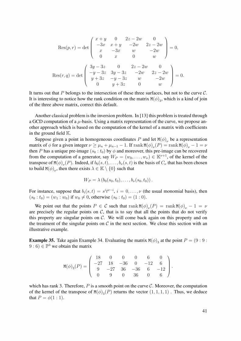
Res(p, r) = det

x+ y 0 2z − 2w 0−3x x+ y −2w 2z − 2wx −3x w −2w0 x 0 w

= 0,

Res(r, q) = det

3y − 3z 0 2z − 2w 0−y − 3z 3y − 3z −2w 2z − 2wy + 3z −y − 3z w −2w

0 y + 3z 0 w

= 0.

It turns out that P belongs to the intersection of these three surfaces, but not to the curve C.It is interesting to notice how the rank condition on the matrix M(φ)3, which is a kind of joinof the three above matrix, correct this default.

Another classical problem is the inversion problem. In [13] this problem is treated througha GCD computation of a µ-basis. Using a matrix representation of the curve, we propose an-other approach which is based on the computation of the kernel of a matrix with coefficientsin the ground field K.

Suppose given a point in homogeneous coordinates P and let M(φ)ν be a representationmatrix of φ for a given integer ν ≥ µn + µn−1 − 1. If rank M(φ)ν(P ) = rank M(φ)ν − 1 = νthen P has a unique pre-image (s0 : t0) by φ and moreover, this pre-image can be recoveredfrom the computation of a generator, say WP = (w0, . . . , wν) ∈ Kν+1, of the kernel of thetranspose of M(φ)ν(P ). Indeed, if b0(s, t), . . . , bν(s, t) is the basis of Cν that has been chosento build M(φ)ν , then there exists λ ∈ K \ 0 such that

WP = λ (b0(s0, t0), . . . , bν(s0, t0)) .

For instance, suppose that bi(s, t) = sitν−i, i = 0, . . . , ν (the usual monomial basis), then(s0 : t0) = (w1 : w0) if w0 6= 0, otherwise (s0 : t0) = (1 : 0).

We point out that the points P ∈ C such that rank M(φ)ν(P ) = rank M(φ)ν − 1 = νare precisely the regular points on C, that is to say that all the points that do not verifythis property are singular points on C. We will come back again on this property and onthe treatment of the singular points on C in the next section. We close this section with anillustrative example.

Example 35. Take again Example 34. Evaluating the matrix M(φ)3 at the point P = (9 : 9 :9 : 6) ∈ P3 we obtain the matrix

M(φ)3(P ) =

18 0 0 0 6 0−27 18 −36 0 −12 69 −27 36 −36 6 −120 9 0 36 0 6

.

which has rank 3. Therefore, P is a smooth point on the curve C. Moreover, the computationof the kernel of the transpose of M(φ)3(P ) returns the vector (1, 1, 1, 1) . Thus, we deducethat P = φ(1 : 1).

41

2.4 Computing the singular points of a rational curve

This section is devoted to the computation of the singular points of a rational curve. Here-after, we will restrict ourselves to the case of rational space curves for simplicity, and alsoto emphasize our new methods in a case which is of particular interest in CAGD. However,all our results can be easily extended to a rational curve in a projective space of arbitrarydimension.

In [18], the authors derive correspondences between the singularities of rational spacecurves and a µ-basis. They also show how to employ µ-bases to compute all the singularitiesof rational space curves of low degree. We propose another approach to compute the singu-larities of rational space curves which is based on the matrix representations introduced inSection 1.2 of the first chapter . It can be seen as an extension of what is called singular fac-tors for the case of rational plane curves in [53]; see also [54]. Remark that the computationof the singular points have been detected in [55] via the generalized resultant method.

2.4.1 Rank of a representation matrix at a singular point

Let C be a rational space curve of degree d ≥ 1 parameterized by the regular map

P1K

φ−→ P3K

(s : t) 7→ (f0 : f1 : f2 : f3)(s, t).

where f0, f1, f2, f3 are four homogeneous polynomials in K[s, t] of the same degree d suchthat their GCD is a nonzero element in K.

Let P be a point on C. There exists at least one point (s1 : t1) ∈ P1 such that P =φ(s1 : t1). Now, let H be a plane in P3 passing through P , not containing C and denote byH(x, y, z, w) an equation (a linear form in K[x, y, z, w]) ofH. We have the following degreed homogeneous polynomial in K[s, t]

H(f0(s, t), f1(s, t), f2(s, t), f3(s, t)) =d∏i=1

(tis− sit) (2.4.1)

where the points (si : ti) ∈ P1, i = 1, . . . , d are not necessarily distinct. We define theintersection multiplicity of C with H at the point P , denoted iP (C,H), as the number ofpoints (si : ti)i=1,...,d such that φ(si : ti) = P .

Definition 36. The multiplicity mP (C) of the point P on C is defined as the minimum of theintersection multiplicity iP (C,H) where H runs over all the hyperplanes not containing Cand passing through the point P ∈ C, minimum which is reached with a sufficiently genericsuchH.

Definition 37. An inversion formula of the point P on C is a homogeneous polynomialhP (s, t) ∈ K[s, t] of degree mp(C) such that hP divides (2.4.1) for any hyperplane H goingthrough P . It is uniquely defined up to multiplication by a nonzero element in K.

42

Given a µ-basis of the parameterization φ, say

p(s, t;x, y, z, w) = p0(s, t)x+ p1(s, t)y + p2(s, t)z + p3(s, t)w,q(s, t;x, y, z, w) = q0(s, t)x+ q1(s, t)y + q2(s, t)z + q3(s, t)w,r(s, t;x, y, z, w) = r0(s, t)x+ r1(s, t)y + r2(s, t)z + r3(s, t)w,

where p, q, r are of degree m ≥ n ≥ l respectively, on can extract an inversion formula of agiven point in P3 with the following result that appears in [18] (we provide here a short prooffor the sake of completeness).

Lemma 38. Let P be a point on C. Then the GCD of the three homogeneous polynomialsp(s, t;P ), q(s, t;P ), r(s, t;P ) in K[s, t] is an inversion formula of P .

Proof. By a linear change of coordinates in P3, one can assume without loss of generalitythat P = (0 : 0 : 0 : 1), because µ-bases have the expected property under linear changeof coordinates. It follows that p(s, t;P ) = p3(s, t), q(s, t;P ) = q3(s, t) and r(s, t;P ) =r3(s, t). Set K(s, t) := gcd(p3, q3, r3).

From the definition of inversion formula we immediately deduce that hP (s, t) :=gcd(f0, f1, f2). So we have to prove that K and hP are equal up to multiplication by anonzero element in K.

From the properties of the µ-basis there exists c ∈ K \ 0 such that

cf0 =

∣∣∣∣∣∣∣p1 p2 p3q1 q2 q3r1 r2 r3

∣∣∣∣∣∣∣ , cf1 = −

∣∣∣∣∣∣∣p0 p2 p3q0 q2 q3r0 r2 r3

∣∣∣∣∣∣∣ , cf2 =

∣∣∣∣∣∣∣p0 p1 p3q0 q1 q3r0 r1 r3

∣∣∣∣∣∣∣ .Therefore, it is clear that K divides hP .

Now, since

p0(s, t)f0(s, t) + p1(s, t)f1(s, t) + p2(s, t)f2(s, t) = −p3(s, t)f3(s, t)

we deduce that hP divides p3f3. But f0, f1, f2 all vanish at the roots of hP so hP and f3cannot share a common root because φ is regular. It follows that hP divides p3. With thesame argument, we get that hP divides q3 and r3 as well. Therefore, hP divides K.

Taking again the notation of Section 1.2, for all integer ν ≥ m + n − 1 we have arepresentation matrix M(φ)ν of the curve C which is built from the µ-basis p, q, r. Its entriesare linear forms in K[x, y, z, w] so that it makes sense to evaluate M(φ)ν at a point in P3 toget a matrix M(φ)ν(P ) with entries in K.

Theorem 39. Given a point P in P3, for all integer ν ≥ m+ n− 1 we have

rank M(φ)ν(P ) = ν + 1−mP (C),

or equivalently corank M(φ)ν(P ) = mP (C).

43

Proof. From Lemma 38, we have that hP (s, t) = gcd(p(s, t;P ), q(s, t;P ), r(s, t;P )) is ahomogeneous polynomial in R := K[s, t] of degree mP (C). From Section 1.2, we recall thatM(φ)ν(P ) is a matrix of the map

R(−m)ν ⊕R(−n)ν ⊕R(−l)ν(p(s,t;P ),q(s,t;P ),r(s,t;P ))−−−−−−−−−−−−−−→ Rν

so that corank M(φ)ν = dimK(R/I)ν for all integer ν, where I stands for the ideal of K[s, t]generated by the polynomials p(s, t;P ), q(s, t;P ) and r(s, t;P ).

Now, the homogeneous polynomials p(s, t;P )/hP , q(s, t;P )/hP , r(s, t;P )/hP are rela-tively prime other K[s, t] so it follows that the saturation of the homogeneous ideal J =(p(s, t;P )/hP , q(s, t;P )/hP , r(s, t;P )/hP ) ⊂ K[s, t] with respect to the ideal m = (s, t)is equal to m. Therefore, we get the following result that we already used: Jν = mν forall ν ≥ m + n − 2mP (C) − 1. But then, multiplying this equality by the homogeneouspolynomial hP we obtain

Iν+mP (C) = hP (p(s, t;P )/hP , q(s, t;P )/hP , r(s, t;P )/hP )ν = (s, t)ν = (hP )ν+mP (C)

for all ν ≥ m+ n− 1− 2mP (C). We conclude that

corank M(φ)ν(P ) = dimK(R/(hP ))ν = ν + 1− (ν −mP (C) + 1) = mP (C)

for all ν ≥ m+n−1−mP (C), which finishes the proof sincemP (C) ≥ 0 for any P ∈ P3.

This result provides a stratification of the points in P3 with respect to the curve C. Indeed,we have that

• if P is such that rank M(φ)ν(P ) = ν + 1 then P 6∈ C,

• if P is such that rank M(φ)ν(P ) = ν then P is a regular point (i.e. of multiplicity 1) onC,

• if P is such that rank M(φ)ν(P ) = ν − 1 then P is singular point of multiplicity 2 onC,

• and so on.

Moreover, an immediate consequence of this theorem and Lemma 38 is that if P is a singularpoint on C then necessarily

2 ≤ mP (C) ≤ n or mP (C) = m. (2.4.2)

We refer the reader to [18] for more results of this kind about the possible singularities on Cwith respect to the µ-basis of its parameterization.

44

2.4.2 Singular factorsTheorem 39 suggests to introduce the singular factors of a representation, similarly to whathas been done in [53], then in [54], for the case of plane curves. Although we are not ableto get results similar to those proved in [54] for plane curves, because the geometry of spacecurves is much less constrained than the one of plane curves, we will nevertheless see thatthese singular factors allow to compute all the singularities of a rational space curve.

As above, suppose given an integer ν ≥ m+n−1 and a representation matrix M(φ)ν of thecurve C which is built from the µ-basis p, q, r of degree m ≥ n ≥ l respectively. We denoteby M(φ)ν(s, t) the matrix M(φ)ν where we substitute x, y, z, w by f0(s, t), f1(s, t), f2(s, t),f3(s, t) respectively. It is then clear that rank M(φ)ν(s, t) < ν + 1 for any point (s : t) ∈ P1.

Definition 40. A collection of homogeneous polynomials d1(s, t), . . . , dν+1(s, t) in K[s, t]such that for all integer i = 1, . . . , ν + 1 the product

dν+1(s, t)ν+1−i+1dν(s, t)ν+1−i · · · di+1(s, t)2di(s, t)

is equal to the GCD of all the (ν + 2 − i)-minors of M(φ)ν(s, t) is called a collection ofsingular factors of the parameterization φ.

Notice that these singular factors are defined up to multiplication by a nonzero elementin K. Moreover, their existence is guaranteed because the ground variety is P1

K, or in otherwords by homogenizing with some care the invariant factors of the matrix M(φ)ν(s, 1), K[s]being a principal ideal domain.

Theorem 41. We have dν+1(s, t) = dν(s, t) = · · · = dm+1(s, t) = 1 and d1(s, t) = 0.Moreover, for any singular point P ∈ C, the inversion formula hP (s, t) divides dmP (C)(s, t)and is coprime with dk(s, t) for all k > mP (C).

Proof. The entries of the matrix M(φ)ν are linear forms in K[x, y, z, w]. Therefore, its de-terminantal ideals, denoted Ik(−) and which correspond to the ideals generated by all thek-minors of M(φ)ν , k = 1, . . . , ν + 1, are homogeneous ideals in K[x, y, z, w].

Then, by using Lemma 38 we deduce that

V (Ik(M(φ)ν)) = ∅ ⊂ P3

for all k = 1, . . . , ν + 1−m, as there cannot be any common factor of degree more than mof the three element of the µ-basis after specialization at a given point. It follows then that

V (Ik(M(φ)ν(s, t))) = ∅ ⊂ P1

for all k = 1, . . . , ν + 1−m, and this implies dk(s, t) = 1 for all k > m.Now, assume for simplicity that P = (0 : 0 : 0 : 1) . As we did above, we have

P /∈ V (Ik(M(φ)ν)) for all k = 1, . . . , ν + 1 − mP (C) which implies that hP (s, t) anddk(s, t) are relatively prime polynomials for all k > mP (C). On the other hand, P ∈V (Iν+1−mP (C)+1(M(φ)ν)), that is Iν+1−mP (C)+1(M(φ)ν) ⊂ (x0, x1, x2), and hence

Iν+1−mP (C)+1(M(φ)ν(s, t)) ⊂ (f0(s, t), f1(s, t), f2(s, t)) ⊂ (hP (s, t)) ⊂ K[s, t].

45

It follows that hP (s, t) divides

dν+1(s, t)ν+1−mP (C)+1 · · · dmP (C)+1(s, t)2dmP (C)(s, t)

and therefore that hP (s, t) divides dmP (C)(s, t).

Here are two consequences of this theorem that allows to characterize the multiplicity ofa singular point and to compute the singular points.

Corollary 42. Let P = φ(s0 : t0) be a point on C, then dmP (C)(s0 : t0) = 0 and dk(s0 :t0) 6= 0 for all k > mP (C). In particular, the multiplicity of P is the highest integer k suchthat dk(s0 : t0) = 0.

Corollary 43. For any integer k such that 2 ≤ k ≤ m, the product∏P∈C : mP (C)=k

hp(s, t)

that runs over all the singular points on C of multiplicity k, divides the singular factordk(s, t).

2.4.3 Computational aspectsThe computation of the singular factors can be done through Smith form computations. In-deed, the matrix M(φ)ν(s, 1) is a matrix with entries in the principal ideal domain K[s].Therefore it is equivalent to the diagonal matrix

dν+1(s, 1)dν+1dν(s, 1)

dν+1dνdν−1(s, 1). . .

dν+1 · · · d3(s, 1)dν+1 · · · d3d2(s, 1)

0

.

So, the computation of this Smith form (or equivalently its invariant factors) yields the de-homogenized singular factors where t is set to 1. It follows that if the point P = φ(1 : 0)is not a singular point, then the singularities of the curve C can be recovered after a singleSmith form computation. If not, it is necessary to either perform the same computation forthe matrix M(φ)ν(1, t) to get the dehomogenized singular factors where now u is set to 1, oreither obtain directly the information on the possible singular point φ(1 : 0) by performingthe GCD computation from Lemma 38.

We conclude this section with two illustrative examples.

Example 44 ( [18, Example 7.6]). Let C be the rational space curve parameterized by

φ : P1K → P3

K : (s : t) 7→ (s5 : s3t2 : s2t3 : t5).

46

A µ-basis for C is given by

p = ty − szq = t2x− s2y,

r = t2z − s2w.

From deg(q) = deg(r) = 2, we can choose ν = 3, then a matrix representation of C isgiven by

M(φ)3 =

y 0 0 x 0 z 0−z y 0 0 x 0 zx −z y −y 0 −w 00 0 −z 0 −y 0 −w

.Substituting x = s5, y = s3t2, z = s2t3, w = t5, we obtain

M(φ)3(s, t) =

s3t2 0 0 s5 0 s2t3 0−s2t3 s3t2 0 0 s5 0 s2t3

0 −s2t3 s3t2 −s3t2 0 −t5 00 0 −s2t3 0 −s3t2 0 −t5

.Now, the Smith form of M(s, 1) and M(1, t) are respectively

1 0 0 0 0 0 00 1 0 0 0 0 00 0 s2 0 0 0 00 0 0 0 0 0 0

and

1 0 0 0 0 0 00 1 0 0 0 0 00 0 t2 0 0 0 00 0 0 0 0 0 0

.Therefore, the singular factors of C are d4(s, t) = 1, d3(s, t) = 1, d2(s, t) = s2t2. Thus, Chas only two singular points of multiplicity 2, the points A = (0 : 0 : 0 : 1) and B = (1 : 0 :0 : 0) that correspond to the parameters (0 : 1) and (1 : 0) respectively.

Example 45. Let C be the classical rational twisted cubic which is parameterized by

φ : P1K → P3

K : (s : t) 7→ (s3 : s2t : st2 : t3).

A µ-basis for C is given by

p = −tx+ sy

q = −ty + sz,

r = −tz + sw.

Since deg(q) = deg(r) = 1, we can choose ν = 1 and then a matrix representation of C is

M(φ)1 =(−x −y −zy z w

).

Substituting x = s3, y = s2t, z = st2, w = t3, we obtain

M(φ)1(s, t) =(−s3 −s2t −st2s2t st2 t3

).

47

The Smith forms of M(s, 1) and M(1, t) are respectively:(1 0 00 0 0

)and

(1 0 00 0 0

).

It follows that the singular factors of C are d3(s, t) = 1, d2(s, t) = 1: we recover the wellknown fact that C has no singular point.

48

Chapter 3

The rational surface/surface intersectionproblems

In the first and second chapters, we introduced and studied the matrix-based implicit rep-resentation of rational surfaces and showed how to use them to compute curve/curve andcurve/surface intersection loci. In this chapter, we extend the approach developed in thesecond chapter for decomposing the parameterized surface/surface intersection locus. Un-like the case of solving the curve/curve and curve/surface intersection problems, addressingthe surface/surface intersection problem by means of matrix representation is much morecomplicated because it requires to compute generalized eigenvalues of bivariate pencils ofmatrices.

Following the approach that we used in the second chapter, to solve the surface/surfaceintersection problem we will develop an algorithm that consists in two main steps. The firstone is the computation of a matrix representation of one of the surface from its parameteriza-tion. After mixing this matrix representation with the parameterization of the other surface,the second step consists in a reduction of a bivariate pencil of matrices and the computationof its continuous and discrete spectrums, via the ∆W − 1 decomposition algorithm that hasbeen introduced by Kublanovskaya in [22].

Throughout this chapter, we assume that C is the field of complex numbers.

3.1 Reduction of a bivariate pencil of matrices

3.1.1 Linearization of a two parameter polynomial matricesLet M(s, t) be a matrix of size m× n depending on the two variables s and t. The spectrumof M(s, t) is defined to be the set

(s0, t0) ∈ C× C : rank(M(s0, t0)) < ρ

where ρ := rankM(s, t). Denote by M j1,...,jρi1,...,iρ the matrix obtained from M(s, t) by taken ρ

rows i1, ..., iρ and ρ columns j1, ..., jρ, 1 ≤ i1 < ... < iρ ≤ m, 1 ≤ j1 < ... < jρ ≤ n. Thecoordinates of its spectrum are the common roots of all the algebraic equations

detM j1,...,jρi1,...,iρ = 0 (3.1.1)

49

The one-dimensional and zero-dimensional roots of the system (3.1.1) determine respec-tively the one-dimensional and zero-dimensional eigenvalues of the matrix M(s, t). Werecall that the one dimensional eigenvalues (also called eigencurves) form the continuouspart of the spectrum which is defined by the equation φ(s, t) = 0 and the zero-dimensionaleigenvalues form the discrete part of the spectrum.

Suppose given an m×n-matrix M(s, t) = (ai,j(s, t)) with polynomial entries ai,j(s, t) ∈C[s, t]. It can be equivalently written as a polynomial in s whose coefficients are m × n-matrices with entries in C[t]: if d = maxi,jdegs(ai,j(s, t)) then

M(s, t) = Md(t)sd +Md−1(t)sd−1 + . . .+M0(s)

where Mi(t) ∈ C[t]m×n.

Definition 46. The generalized companion matrices A(t), B(t) of the matrix M(s, t) are thematrices with coefficients in C[t] of size ((d− 1)m+ n)× dm that are given by

A(t) =

0 I . . . . . . 00 0 I . . . 0...

......

......

0 0 . . . . . . IM t

0(t) M t1(t) . . . . . . M t

d−1(t)

B =

I 0 . . . . . . 00 I 0 . . . 0...

......

......

0 0 . . . I 00 0 . . . . . . −M t

d(t)

where I stands for the identity matrix andM t

i (t) stands for the transpose of the matrixMi(t).

We have the following interesting property that follows from a straightforward computa-tion.

Proposition 47. With the above notation, for all s ∈ C and all vector v ∈ C[t]m we have

M t(s, t)v = 0⇔ (A(t)− sB(t))

vsv...

sd−1v

= 0.

In particular, these companion matrices allows to linearize the polynomial matrix M(s, t)in the sense that there exists two unimodular matrices E(s, t) et F (s, t) with coefficients inC[s, t] and of size dm and (d− 1)m+ n respectively, such that

E(s, t) (A(t)− sB(t))F (s, t) =(

tM(s, t) 00 Id(m−1)

). (3.1.2)

So, we obtain

50

Theorem 48. The spectrum of the matrix M(s, t) and the spectrum of the pencil matrixA(t)− sB(t) coincide.

By Theorem 48, we transform the computation of the spectrum of the polynomial matrixM(s, t) into the computation of the spectrum of a bivariate pencil of matrices A(t)− sB(t).If the matrices A(t), B(t) are two square matrices, we could compute the spectrum of thepolynomial matrix M(s, t) as the roots of the algebraic equation detM(s, t) = 0. There-fore, our next task is to reduce the pencil A(t) − sB(t) into a regular pencil that keeps theinformation we are interested in.

3.1.2 The ∆W − 1 DecompositionIn this part, we present an algorithm, called the ∆W − 1 decomposition, that has beenintroduced by Kublanovskaya in [22]. Its purpose is to transform an univariate polynomialmatrix M(t) into the form [∆(t), 0] where ∆(t) is a polynomial matrix of full column rankand 0 is a zero block-matrix. Notice that the presentation of the decomposition algorithm isvery hard to follow in [22]. Hereafter, we try to present it more clearly with some illustrativeexamples.

Suppose given a polynomial matrix M(t) of size m× n and write it under the form

M(t) =[Ms,1, 0, 0, . . . , 0]ts + [Ms−1,1,Ms−1,2, 0, . . . , 0]ts−1 + . . .

+[Ms−p+2,1, . . . ,Ms−p+2,p−1, 0]ts−p+2 + [Ms−p+1,1, . . . ,Ms−p+1,p−1,Ms−p+1,p]ts−p+1

+[Ms−p,1, . . . ,Ms−p,p−1,Ms−p,p]ts−p + . . .+ [M01,M02, . . . ,M0p]

where 1 ≤ p ≤ s+ 1 and for each i, i = 1, 2, . . . , p, the block matrices Mj,i, j = 0, 1, . . . , shave the same size m× ti ,

p∑i=1

ti = n and 0 stands for the zero block-matrix.

Lemma 49. If the matrix M = [Ms,1,Ms−1,2, . . . ,Ms−p+1,p] is of full column rank, thematrix M(t) is of full column rank.

Proof. Suppose that the matrix M(t) is not of full column rank, there exists a polynomialvector F (t) ∈ C[t]n×1, F (t) 6= 0 such that M(t)F (t) = 0. Let k := maxjdegt fi(t), j =1, 2, . . . , n, we have

F (t) = Fktk + Fk−1t

k−1 + . . .+ F0

where Fi = (Fi1, Fi2, . . . , Fin)t ∈ Cn×1, i = 0, 1, . . . , k and Fk 6= 0. From

M(t)F (t) = 0 = [Ms,1, 0, 0, . . . , 0]Fkts+k + ([Ms−1,1,Ms−1,2, 0, . . . , 0]Fk + [Ms1, 0, 0, . . . , 0]Fk−1)ts+k−1

+ ([Ms1, 0, 0, . . . , 0]Fk−2 + [Ms−1,1,Ms−1,2, 0, . . . , 0]Fk−1 + [Ms−2,1,Ms−2,2,Ms−2,3, . . . , 0]Fk)ts+k−2

+ . . .+ [M01,M02, . . . ,M0p]F0

for every t ∈ C, we deduce that the coefficients with respect to the variable t of thematrix M(t)F (t) are null matrices. By the independence of the columns of the matrixM = [Ms,1,Ms−1,2, . . . ,Ms−p+1,p] and looking at the coefficient of ts+k, ts+k−1, . . . we ob-tain that necessarily

Fk,1 = Fk,2 = . . . = Fk,t1 = 0,Fk,t1+1 = Fk,t1+2 = . . . = Fk,t1+t2 = Fk−1,1 = Fk−1,2 = . . . = Fk−1,t1 = 0................................................

51

Finally, we arrive at the conclusion that Fk has to be the null vector which gives a contradic-tion.

Corollary 50. LetM(t) = tsMs + ts−1Ms−1 + . . .+M0

be an univariate polynomial matrix of size m× n. If Ms is of full column rank then M(t) isof full column rank.

Proof. Apply Lemma 49 where the decomposition of M(t) is taken with p = 1.

Suppose given an univariate polynomial m × n matrix of rank ρ and degree s ≥ 1 withm× n constant matrices M0,M1, . . . ,Ms

M(t) = tsMs + ts−1Ms−1 + . . .+M0.

The decomposition of M(t) under the form

M(t)W (t) = [∆(t), 0] (3.1.3)

is called the ∆W−1 decomposition, whereW (t) is an n×n unimodular polynomial matrix,∆(t) is an m × ρ polynomial matrix of full column rank whose degree does not exceed s,0 is an m × (n − ρ) zero matrix. The ∆W − 1 decomposition algorithm computes thesequence of polynomial matrices M0(t) = M(t),M1(t), . . . ,Ml(t) where Ml(t) = [∆(t), 0]and Mk(t) = Mk−1(t)Wk(t), Wk(t) is an unimodular matrix, k = 1, 2, . . . , l.

Now, we are ready to describe the ∆W − 1 decomposition algorithm:

Step 1 Construct an auxiliary matrix N1 as follows.

(i) if all the columns of Ms are nonzero then N1 := Ms. Otherwise, Ms contains somezero columns. By column permutations, we can transform Ms into M∗

s := [Ms,1, 0]where Ms1 is the nonzero columns of Ms of size m × t1, so the coefficient matricesMq are permuted with the form M∗

q := [Mq,1,Mq,2], q = s− 1, . . . , 0 where Mq1,Mq2are respectively the m× t1 and m× (n− t1).

(ii) If all the columns of Ms−1,2 are nonzero, then

N1 := [Ms,1,Ms−1,2].

Otherwise, the columns of the coefficient matrices Mq,2, q = s − 1, .., 0 can be per-muted to get M∗

s−1,2 := [Ms−1,2, 0] where Ms−1,2 is the nonzero columns of Ms−1,2of size m × t2 and M∗

q,2 := [Mq,2,Mq,3], q = s − 2, . . . , 0. The blocks Mq,2,Mq,3 arerespectively of size m× t2 and m× (n− t1 − t2).

(iii) if all the columns of Ms−2,3 are nonzero, then

N1 := [Ms,1, Ms−1,2,Ms−2,3]

52

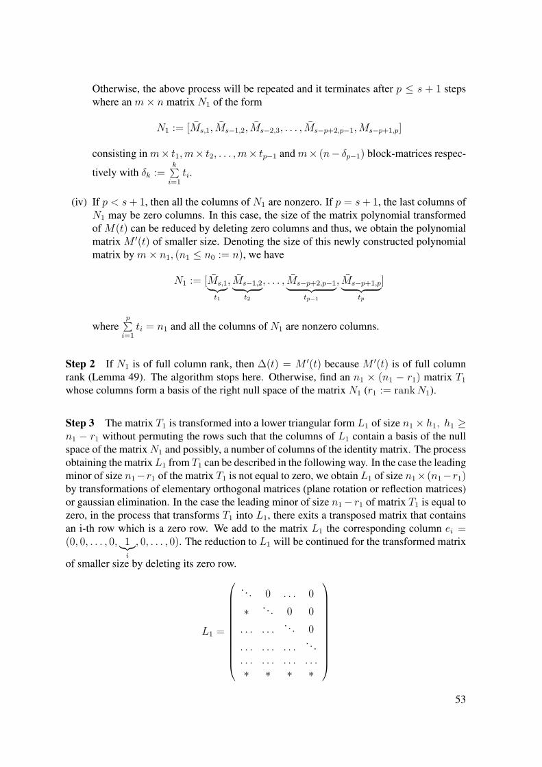
Otherwise, the above process will be repeated and it terminates after p ≤ s + 1 stepswhere an m× n matrix N1 of the form

N1 := [Ms,1, Ms−1,2, Ms−2,3, . . . , Ms−p+2,p−1,Ms−p+1,p]

consisting in m× t1,m× t2, . . . ,m× tp−1 and m× (n− δp−1) block-matrices respec-

tively with δk :=k∑i=1

ti.

(iv) If p < s+ 1, then all the columns of N1 are nonzero. If p = s+ 1, the last columns ofN1 may be zero columns. In this case, the size of the matrix polynomial transformedof M(t) can be reduced by deleting zero columns and thus, we obtain the polynomialmatrix M ′(t) of smaller size. Denoting the size of this newly constructed polynomialmatrix by m× n1, (n1 ≤ n0 := n), we have

N1 := [Ms,1︸ ︷︷ ︸t1

, Ms−1,2︸ ︷︷ ︸t2

, . . . , Ms−p+2,p−1︸ ︷︷ ︸tp−1

, Ms−p+1,p︸ ︷︷ ︸tp

]

wherep∑i=1

ti = n1 and all the columns of N1 are nonzero columns.

Step 2 If N1 is of full column rank, then ∆(t) = M ′(t) because M ′(t) is of full columnrank (Lemma 49). The algorithm stops here. Otherwise, find an n1 × (n1 − r1) matrix T1whose columns form a basis of the right null space of the matrix N1 (r1 := rankN1).

Step 3 The matrix T1 is transformed into a lower triangular form L1 of size n1 × h1, h1 ≥n1 − r1 without permuting the rows such that the columns of L1 contain a basis of the nullspace of the matrixN1 and possibly, a number of columns of the identity matrix. The processobtaining the matrixL1 from T1 can be described in the following way. In the case the leadingminor of size n1−r1 of the matrix T1 is not equal to zero, we obtain L1 of size n1×(n1−r1)by transformations of elementary orthogonal matrices (plane rotation or reflection matrices)or gaussian elimination. In the case the leading minor of size n1− r1 of matrix T1 is equal tozero, in the process that transforms T1 into L1, there exits a transposed matrix that containsan i-th row which is a zero row. We add to the matrix L1 the corresponding column ei =(0, 0, . . . , 0, 1︸︷︷︸

i

, 0, . . . , 0). The reduction to L1 will be continued for the transformed matrix

of smaller size by deleting its zero row.

L1 =

. . . 0 . . . 0∗ . . . 0 0. . . . . .

. . . 0. . . . . . . . .

. . .. . . . . . . . . . . .∗ ∗ ∗ ∗

53

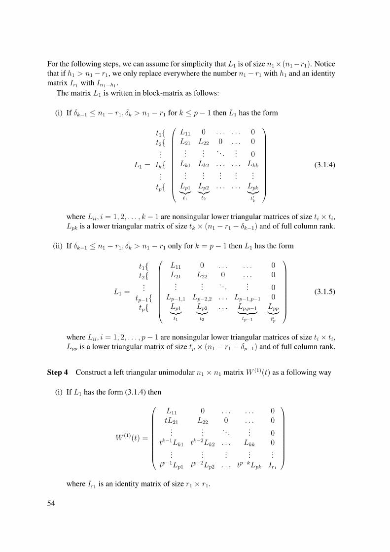
For the following steps, we can assume for simplicity that L1 is of size n1×(n1−r1). Noticethat if h1 > n1− r1, we only replace everywhere the number n1− r1 with h1 and an identitymatrix Ir1 with In1−h1 .

The matrix L1 is written in block-matrix as follows:

(i) If δk−1 ≤ n1 − r1, δk > n1 − r1 for k ≤ p− 1 then L1 has the form

L1 =

t1t2...tk

...tp

L11 0 . . . . . . 0L21 L22 0 . . . 0

...... . . . ... 0

Lk1 Lk2 . . . . . . Lkk...

......

......

Lp1︸︷︷︸t1

Lp2︸︷︷︸t2

. . . . . . Lpk︸︷︷︸t′k

(3.1.4)

where Lii, i = 1, 2, . . . , k − 1 are nonsingular lower triangular matrices of size ti × ti,Lpk is a lower triangular matrix of size tk × (n1 − r1 − δk−1) and of full column rank.

(ii) If δk−1 ≤ n1 − r1, δk > n1 − r1 only for k = p− 1 then L1 has the form

L1 =

t1t2...

tp−1tp

L11 0 . . . . . . 0L21 L22 0 . . . 0

...... . . . ... 0

Lp−1,1 Lp−2,2 . . . Lp−1,p−1 0Lp1︸︷︷︸t1

Lp2︸︷︷︸t2

. . . Lp,p−1︸ ︷︷ ︸tp−1

Lpp︸︷︷︸t′p

(3.1.5)

where Lii, i = 1, 2, . . . , p− 1 are nonsingular lower triangular matrices of size ti × ti,Lpp is a lower triangular matrix of size tp × (n1 − r1 − δp−1) and of full column rank.

Step 4 Construct a left triangular unimodular n1 × n1 matrix W (1)(t) as a following way

(i) If L1 has the form (3.1.4) then

W (1)(t) =

L11 0 . . . . . . 0tL21 L22 0 . . . 0

...... . . . ... 0

tk−1Lk1 tk−2Lk2 . . . Lkk 0...

......

......

tp−1Lp1 tp−2Lp2 . . . tp−kLpk Ir1

where Ir1 is an identity matrix of size r1 × r1.

54

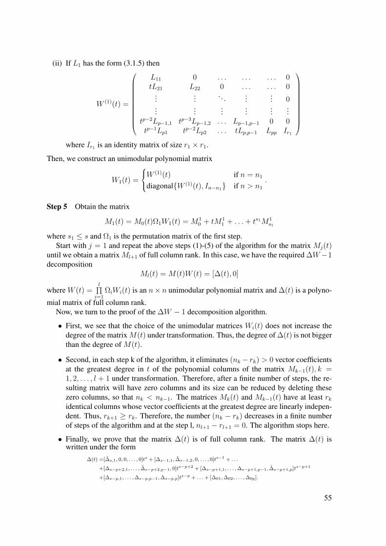
(ii) If L1 has the form (3.1.5) then

W (1)(t) =

L11 0 . . . . . . . . . 0tL21 L22 0 . . . . . . 0

...... . . . ...

... 0...

......

......

...tp−2Lp−1,1 tp−3Lp−1,2 . . . Lp−1,p−1 0 0tp−1Lp1 tp−2Lp2 . . . tLp,p−1 Lpp Ir1

where Ir1 is an identity matrix of size r1 × r1.

Then, we construct an unimodular polynomial matrix

W1(t) =

W (1)(t) if n = n1

diagonalW (1)(t), In−n1 if n > n1.

Step 5 Obtain the matrix

M1(t) = M0(t)Ω1W1(t) = M10 + tM1

1 + . . .+ ts1M1s1

where s1 ≤ s and Ω1 is the permutation matrix of the first step.Start with j = 1 and repeat the above steps (1)-(5) of the algorithm for the matrix Mj(t)

until we obtain a matrixMl+1 of full column rank. In this case, we have the required ∆W−1decomposition

Ml(t) = M(t)W (t) = [∆(t), 0]

where W (t) =l∏

i=1ΩiWi(t) is an n× n unimodular polynomial matrix and ∆(t) is a polyno-

mial matrix of full column rank.Now, we turn to the proof of the ∆W − 1 decomposition algorithm.

• First, we see that the choice of the unimodular matrices Wi(t) does not increase thedegree of the matrixM(t) under transformation. Thus, the degree of ∆(t) is not biggerthan the degree of M(t).

• Second, in each step k of the algorithm, it eliminates (nk − rk) > 0 vector coefficientsat the greatest degree in t of the polynomial columns of the matrix Mk−1(t), k =1, 2, . . . , l + 1 under transformation. Therefore, after a finite number of steps, the re-sulting matrix will have zero columns and its size can be reduced by deleting thesezero columns, so that nk < nk−1. The matrices Mk(t) and Mk−1(t) have at least rkidentical columns whose vector coefficients at the greatest degree are linearly indepen-dent. Thus, rk+1 ≥ rk. Therefore, the number (nk − rk) decreases in a finite numberof steps of the algorithm and at the step l, nl+1 − rl+1 = 0. The algorithm stops here.

• Finally, we prove that the matrix ∆(t) is of full column rank. The matrix ∆(t) iswritten under the form

∆(t) =[∆s,1, 0, 0, . . . , 0]ts + [∆s−1,1, ∆s−1,2, 0, . . . , 0]ts−1 + . . .

+[∆s−p+2,1, . . . , ∆s−p+2,p−1, 0]ts−p+2 + [∆s−p+1,1, . . . ,∆s−p+1,p−1, ∆s−p+1,p]ts−p+1

+[∆s−p,1, . . . ,∆s−p,p−1,∆s−p,p]ts−p + . . .+ [∆01,∆02, . . . ,∆0p].

55

By construction, the matrix Nl+1 = [∆s,1, ∆s−1,2, . . . , ∆s−p+1,p] is of full columnrank. By Lemma 49, the ∆(t) is of full column rank.

Remark 51. In the second chapter, we used the LU-decomposition to transform easily anarbitrary constant matrix A to a matrix under the form [A1|0] where A1 is of full columnrank. However, this algorithm can not be applied to a polynomial matrix M(t) because theoperations of the transformation of M(t) have been done over the polynomial ring C[t], notthe field C. Thus, the ∆W −1 decomposition algorithm is required although it is much morecomplicated.Now, we give some examples to illustrate the above algorithm.

Example 52. Let M(t) be an univariate polynomial matrix

M(t) :=

2t2 + 3t+ 1 t+ 1 2t2 + 2t

1 5t2 −5t2 + 12t+ 1 3 2t− 2t t 0

= M2t2 +M1t

1 +M0

where

M2 =

2 0 20 5 −50 0 00 0 0

,M1 =

3 1 20 0 02 0 21 1 0

,M0 =

1 1 01 0 11 3 −20 0 0

.From all columns of the matrix M2 are nonzero columns, we choose N1 := M2 and then

the null space of N1 is L1 := [1,−1,−1]t. So we construct the matrix

W (1)(t) =

1 0 0−1 1 0−1 0 1

.We have

M1(t) = M(t)W (1)(t) =

0 t+ 1 2t2 + 2t0 5t2 −5t2 + 10 3 2t− 20 t 0

.

From the coefficient matrix of greatest degree of the matrix ∆(t) :=

t+ 1 2t2 + 2t5t2 −5t2 + 13 2t− 2t 0

is

0 25 −50 00 0

of full column rank. By Corollary 50, the matrix ∆(t) is of full column rank.

Example 53. Let M(t) be an univariate polynomial matrix

M(t) :=

−t 0 t2 1 + t3

0 −t −1 + t3 −t2t2 1 + t3 t 0

= M3t3 +M2t

2 +M1t+M0

56

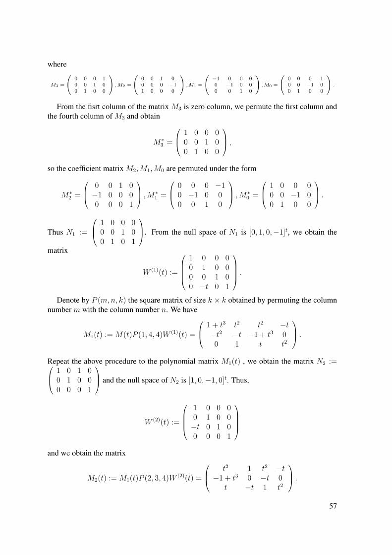
where

M3 =

(0 0 0 10 0 1 00 1 0 0

),M2 =

(0 0 1 00 0 0 −11 0 0 0

),M1 =

(−1 0 0 00 −1 0 00 0 1 0

),M0 =

(0 0 0 10 0 −1 00 1 0 0

).

From the fisrt column of the matrix M3 is zero column, we permute the first column andthe fourth column of M3 and obtain

M∗3 =

1 0 0 00 0 1 00 1 0 0

,so the coefficient matrix M2,M1,M0 are permuted under the form

M∗2 =

0 0 1 0−1 0 0 00 0 0 1

,M∗1 =

0 0 0 −10 −1 0 00 0 1 0

,M∗0 =

1 0 0 00 0 −1 00 1 0 0

.

Thus N1 :=

1 0 0 00 0 1 00 1 0 1

. From the null space of N1 is [0, 1, 0,−1]t, we obtain the

matrix

W (1)(t) :=

1 0 0 00 1 0 00 0 1 00 −t 0 1

.Denote by P (m,n, k) the square matrix of size k × k obtained by permuting the column

number m with the column number n. We have

M1(t) := M(t)P (1, 4, 4)W (1)(t) =

1 + t3 t2 t2 −t−t2 −t −1 + t3 00 1 t t2

.Repeat the above procedure to the polynomial matrix M1(t) , we obtain the matrix N2 := 1 0 1 0

0 1 0 00 0 0 1

and the null space of N2 is [1, 0,−1, 0]t. Thus,

W (2)(t) :=

1 0 0 00 1 0 0−t 0 1 00 0 0 1

and we obtain the matrix

M2(t) := M1(t)P (2, 3, 4)W (2)(t) =

t2 1 t2 −t−1 + t3 0 −t 0

t −t 1 t2

.57

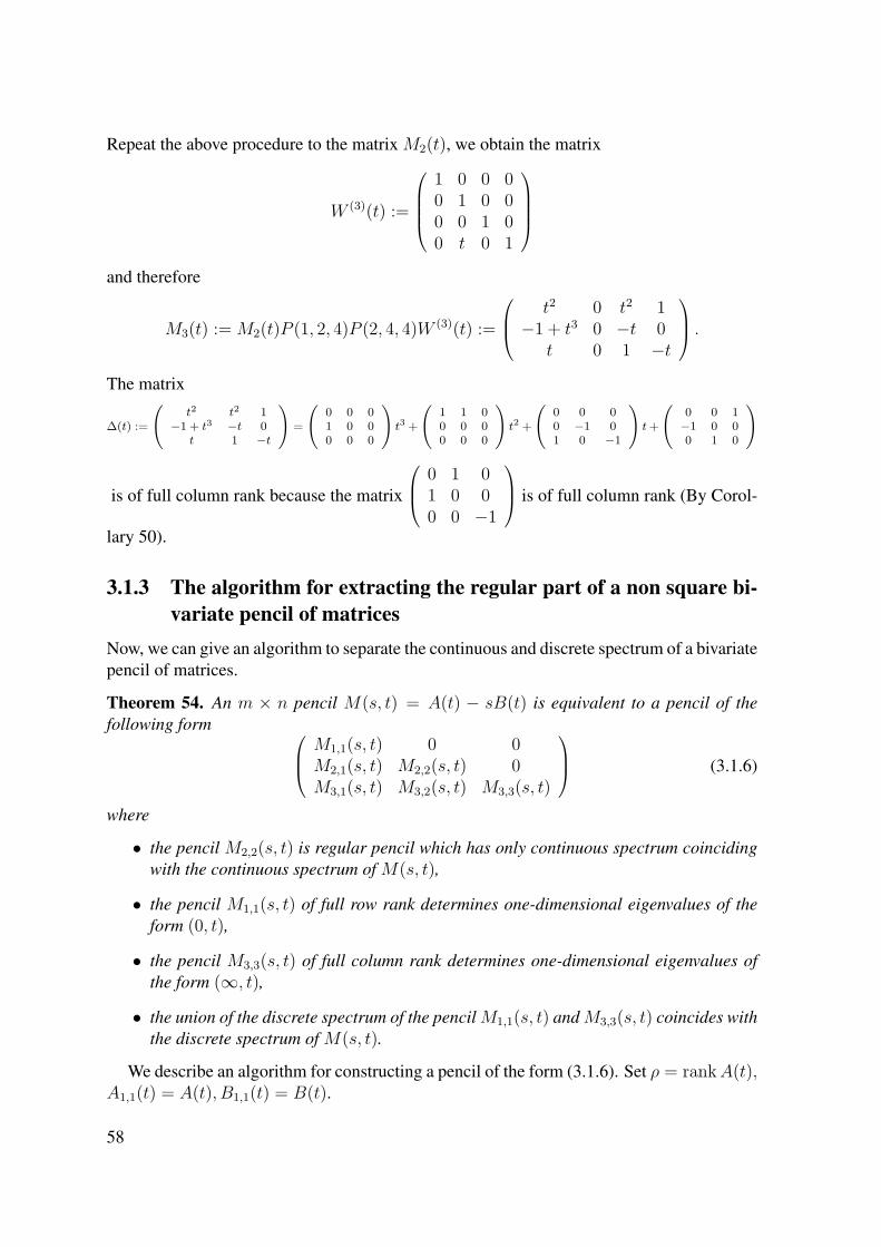
Repeat the above procedure to the matrix M2(t), we obtain the matrix

W (3)(t) :=

1 0 0 00 1 0 00 0 1 00 t 0 1

and therefore

M3(t) := M2(t)P (1, 2, 4)P (2, 4, 4)W (3)(t) :=

t2 0 t2 1−1 + t3 0 −t 0

t 0 1 −t

.The matrix

∆(t) :=

(t2 t2 1

−1 + t3 −t 0t 1 −t

)=

(0 0 01 0 00 0 0

)t3 +

(1 1 00 0 00 0 0

)t2 +

(0 0 00 −1 01 0 −1

)t+

(0 0 1−1 0 00 1 0

)

is of full column rank because the matrix

0 1 01 0 00 0 −1

is of full column rank (By Corol-

lary 50).

3.1.3 The algorithm for extracting the regular part of a non square bi-variate pencil of matrices

Now, we can give an algorithm to separate the continuous and discrete spectrum of a bivariatepencil of matrices.

Theorem 54. An m × n pencil M(s, t) = A(t) − sB(t) is equivalent to a pencil of thefollowing form M1,1(s, t) 0 0

M2,1(s, t) M2,2(s, t) 0M3,1(s, t) M3,2(s, t) M3,3(s, t)

(3.1.6)

where

• the pencil M2,2(s, t) is regular pencil which has only continuous spectrum coincidingwith the continuous spectrum of M(s, t),

• the pencil M1,1(s, t) of full row rank determines one-dimensional eigenvalues of theform (0, t),

• the pencil M3,3(s, t) of full column rank determines one-dimensional eigenvalues ofthe form (∞, t),

• the union of the discrete spectrum of the pencilM1,1(s, t) andM3,3(s, t) coincides withthe discrete spectrum of M(s, t).

We describe an algorithm for constructing a pencil of the form (3.1.6). Set ρ = rankA(t),A1,1(t) = A(t), B1,1(t) = B(t).

58

Step 1

i) Transform A1,1(t) into the form [∆0(t), 0] by the ∆W − 1 decomposition that means

A1,1(t)Q0(t) = [∆0(t), 0]

where Q0(t) is an unimodular matrix. Then, compute

B1,1(t)Q0(t) = [B1(t)︸ ︷︷ ︸ρ

|B2(t)︸ ︷︷ ︸n−ρ

]

.

ii) Determine an unimodular matrix P0(t) such that

P0(t)B2(t) =(B1,1(t)

0

)

where B1,1(t) has full row rank. At the end of ii), matrices A(t) and B(t) are repre-sented under the form

P0(t)A1,1(t)Q0(t) =(A2,1(t) 0A2,2(t) 0

), P0(t)B1,1(t)Q0(t) =

(B2,1(t) B1,1(t)B2,2(t) 0

)

where- B1,1(t) has full row rank.

-(A2,1(t)A2,2(t)

)has full column rank.

We have

P0(t)(A1,1(t)− sB1,1(t))Q0(t) =(A2,1(t)− sB2,1(t) −sB1,1(t)A2,2(t)− sB2,2(t) 0

)

iii) By the permutation of block rows, we obtain the matrix

PP0(t)(A1,1(t)− sB1,1(t))Q0(t) =(A2,2(t)− sB2,2(t) 0A2,1(t)− sB2,1(t) −sB1,1(t)

)

where P is a matrix of this permutation.

Step 2 If the matrix A2,2(t) is not of full column rank, we repeat the Step 1 for the pencilA2,2(t)− sB2,2(t) until the step k where the matrix Ak+1,k+1(t) is of full column rank. Thus,we have the pencil

P (t)M(s, t)Q(t) =(Ak+1,k+1(t)− sBk+1,k+1(t) 0Ak+1,k(t)− sBk+1,k(t) M3,3(s, t)

)

where P (t), Q(t) are unimodular matrices.If the pencil of the m1 × n1 matrix Ak+1,k+1(t) − sBk+1,k+1(t) is not regular pencil so

it is not square matrix and not of full row rank, then we repeat the above procedure to thetransposed pencilAtk+1,k+1(t)−sBt

k+1,k+1(t). For instance, the steps consist in the followingoperations: Set A1,1(t) = Ak+1,k+1(t), B1,1(t) = Bk+1,k+1(t)

59

i) Transform the transpose matrix Bt1,1(t) into the form [∆0(t), 0] that means

Bt1,1(t)Q0(t) = [∆0(t)︸ ︷︷ ︸

ρ

| 0︸︷︷︸m1−ρ

]

where Q0(t) is an unimodular matrix and ρ = rank Bt1,1(t). Then, compute

Qt0(t)(A1,1(t)− sB1,1(t)) =

(A2(t)− sB2(t)

A1(t)

)

where B2(t) = ∆t0(t).

ii) Determine unimodular matrix P0(t) such that

A1(t)P0(t) =(A1,1(t) 0

)where A1,1(t) is an ρ × q matrix of full columns rank. At the end of ii), the pencilA1,1(t)− sB1,1(t) is represented under the form

Qt0(t)(A1,1(t)− sB1,1(t))P0(t) =

(A2,1(t)− sB2,1(t) A2,2(t)− sB2,2(t)

A1,1(t) 0

)

iii) By the permutation of block columns, we obtain the matrix

Qt0(t)(A1,1(t)− sB1,1(t))P0(t)C =

(A2,2(t)− sB2,2(t) A2,1(t)− sB2,1(t)

0 A1,1(t)

)

where C is a matrix of this permutation.

If the matrix B2,2(t) is not of full row rank, we repeat the above procedure to thepencil A2,2(t) − sB2,2(t) until the step l where the matrix Bl+1,l+1(t) is of full rowrank. Hence, we obtain the regular pencil Al+1,l+1(t)− sBl+1,l+1(t).At the end, we obtain the following pencil equivalent to M(s, t)

P (t)M(s, t)Q(t) =

M1,1(s, t) 0 0M2,1(s, t) M2,2(s, t) 0M3,1(s, t) M3,2(s, t) M3,3(s, t)

where P (t), Q(t) are unimodular matrices.

The pencil M2,2(t) = Al+1,l+1(t)− sBl+1,l+1(t) is the regular pencil. The pencil

M1,1(t) =

Al,l(t) Al,l−1(t)− sBl,l−1(t) . . . Al,1(t)− sBl,1(t)

0 Al−1,l−1(t) . . . Al−1,1(t)− sBl−1,1(t)0 0 . . . ...0 . . . 0 A1,1(t)

60

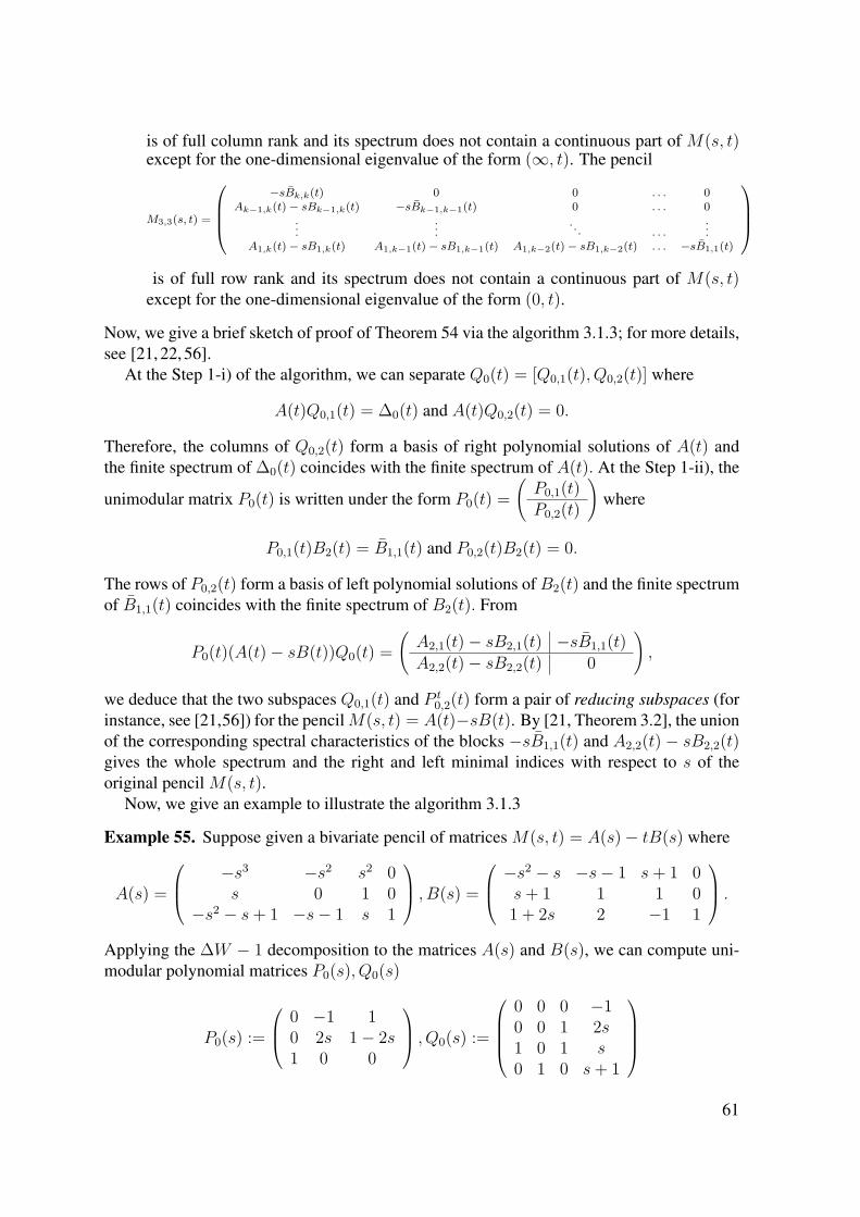
is of full column rank and its spectrum does not contain a continuous part of M(s, t)except for the one-dimensional eigenvalue of the form (∞, t). The pencil

M3,3(s, t) =

−sBk,k(t) 0 0 . . . 0

Ak−1,k(t)− sBk−1,k(t) −sBk−1,k−1(t) 0 . . . 0...

.... . . . . .

...A1,k(t)− sB1,k(t) A1,k−1(t)− sB1,k−1(t) A1,k−2(t)− sB1,k−2(t) . . . −sB1,1(t)

is of full row rank and its spectrum does not contain a continuous part of M(s, t)

except for the one-dimensional eigenvalue of the form (0, t).

Now, we give a brief sketch of proof of Theorem 54 via the algorithm 3.1.3; for more details,see [21, 22, 56].

At the Step 1-i) of the algorithm, we can separate Q0(t) = [Q0,1(t), Q0,2(t)] where

A(t)Q0,1(t) = ∆0(t) and A(t)Q0,2(t) = 0.

Therefore, the columns of Q0,2(t) form a basis of right polynomial solutions of A(t) andthe finite spectrum of ∆0(t) coincides with the finite spectrum of A(t). At the Step 1-ii), the

unimodular matrix P0(t) is written under the form P0(t) =(P0,1(t)P0,2(t)

)where

P0,1(t)B2(t) = B1,1(t) and P0,2(t)B2(t) = 0.

The rows of P0,2(t) form a basis of left polynomial solutions of B2(t) and the finite spectrumof B1,1(t) coincides with the finite spectrum of B2(t). From

P0(t)(A(t)− sB(t))Q0(t) =(A2,1(t)− sB2,1(t) −sB1,1(t)A2,2(t)− sB2,2(t) 0

),

we deduce that the two subspaces Q0,1(t) and P t0,2(t) form a pair of reducing subspaces (for

instance, see [21,56]) for the pencilM(s, t) = A(t)−sB(t). By [21, Theorem 3.2], the unionof the corresponding spectral characteristics of the blocks −sB1,1(t) and A2,2(t) − sB2,2(t)gives the whole spectrum and the right and left minimal indices with respect to s of theoriginal pencil M(s, t).

Now, we give an example to illustrate the algorithm 3.1.3

Example 55. Suppose given a bivariate pencil of matrices M(s, t) = A(s)− tB(s) where

A(s) =

−s3 −s2 s2 0s 0 1 0

−s2 − s+ 1 −s− 1 s 1

, B(s) =

−s2 − s −s− 1 s+ 1 0

s+ 1 1 1 01 + 2s 2 −1 1

.Applying the ∆W − 1 decomposition to the matrices A(s) and B(s), we can compute uni-modular polynomial matrices P0(s), Q0(s)

P0(s) :=

0 −1 10 2s 1− 2s1 0 0

, Q0(s) :=

0 0 0 −10 0 1 2s1 0 1 s0 1 0 s+ 1

61

such that

A1(s) := P0(s)A(s)Q0(s) =

−1 + s 1 −2 03s− 2s2 1− 2s −1 + 4s 0

s2 0 0 0

B1(s) := P0(s)B(s)Q0(s) =

−2 1 −1 1−1 + 4s 1− 2s 1 + 2s 0s+ 1 0 0 0

.Therefore, we obtain the matricesA2(s) :=

(3s− 2s2 1− 2s −1 + 4s

s2 0 0

)andB2(s) :=(

−1 + 4s 1− 2s 1 + 2ss+ 1 0 0

). Applying the ∆W −1 decomposition to the matrices A2(s)

and B2(s), we compute the unimodular polynomial matrices P1(s) and Q1(s)

P1(s) :=(

1 00 1

), Q1(s) :=

1 0 00 1 2− 8s0 1/2 2− 4s

such that

A3(s) := P1(s)A2(s)Q1(s) =(

3s− 2s2 12 0

s2 0 0

)

B3(s) := P1(s)A2(s)Q1(s) =(−1 + 4s 3

2 − s 4− 12s+ 8s2

s+ 1 0 0

).

At last, we can transform the pencil of matrices M(s, t) into the matrix form −1 + s 1 −2 03s− 2s2 1

2 0 0s2 0 0 0

− t −2 1 −1 1−1 + 4s 3

2 − s 4− 12s+ 8s2 0s+ 1 0 0 0

where M1(s, t) := [s2] − t[s + 1] is a regular pencil part of the pencil matrix M(s, t) and

M2(s, t) :=(

1 −2 012 0 0

)− t

(1 −1 1

32 − s 4− 12s+ 8s2 0

)of full row rank determines

the discrete spectrum of M(s, t). Hence, the one-dimensional eigenvalue of M(s, t) is s2 −t(s+ 1) and the zero-dimensional eigenvalue of M(s, t) is the pair (1, 1).

3.1.4 An algorithm for constructing the discrete spectrumConsider M(s, t) = A(t) − sB(t) an m × n (m > n) pencil of full rank n that is free ofcontinuous spectrum. Now, we present an algorithm for obtaining the discrete spectrum ofM(s, t).

Step 1 We construct a polynomial matrix Λ(t) := [A(t),−B(t)] and compute a generalizedeigenvalue t∗ of Λ(t).

62

Step 2 For each generalized eigenvalue t∗, we compute two matrices Q−, Q+ which areconstant matrices of the first n and the last n rows of the matrix Q∗ whose columns form abasis of the right null space of the constant matrix Λ(t∗).

Step 3 We compute a generalized eigenvalue s∗ of the pencil matrix M1(s) := Q−− sQ+.Then (s∗, t∗) is a zero-dimensional eigenvalue of the pencil M(s, t).

Now, we give a brief proof of the algorithm 3.1.4 (for more details, see [21, 22]). First,

we construct a pencil matrix M1(s, t) = A1(t) − sB1(t) such that(B1(t)A1(t)

)forms a basis

of the right null space of Λ(t). Indeed,

M1(s, t) =

W−(t)− sW+(t) if t 6= t∗

Q− − sQ+ if t = t∗

where t∗ is a fixed generalized eigenvalue of the polynomial matrix Λ(t). The matricesW−(t) and W+(t) are polynomial matrices composed of the first n and the last n rows ofthe matrix W0(t) whose columns form a minimal basis for the right null space of Λ(t). Thematrices Q− and Q+ are constant matrices composed of the first n and the last n rows ofthe matrix Q∗ whose columns form a minimal basis for the right null space of the constantmatrix Λ(t∗). Thus, we have

• Each zero-dimensional eigenvalue (s∗, t∗) of the pencilM1(s, t) is also a zero-dimensionaleigenvalue (s∗, t∗) of the pencil M(s, t) and the corresponding eigenvectors x∗ and y∗of the pencils M(s, t) and M1(s, t) respectively satisfy the following relations:

x∗ = Q+y∗, y∗ = Qt∗

(x∗sx∗

).

• A pair (s∗, t∗) is a zero-dimensional eigenvalue of the pencil M(s, t) if t∗ is a gen-eralized eigenvalue of the polynomial matrix Λ(t) and s∗ is a generalized eigenvalueof the pencil M1(s, t∗). This property is deduced from the fact that if y∗ is an eigen-vector corresponding to the generalized eigenvalue s∗ of the pencil M(s∗, t∗) thenM(s∗, t∗)y∗ ≡ (Q− − s∗Q+)y∗ = 0 so that y∗ is also an eigenvector corresponding tothe generalized eigenvalue s∗ of the pencil M1(s, t∗).

Remark 56.

i) The polynomial matrix W0(t) can be computed by finding the ∆W − 1 decompositionof the matrix Λ(t), Λ(t)W (t) = [∆(t), 0] where ∆(t) is of full column rank and W (t) =[W1(t),W2(t) is an unimodular matrix. The matrices W1(t) and W2(t) are of size 2n × ρand 2n× (2n−ρ), respectively (ρ := rank Λ(t)). The matrix W2(t) form a basis of the rightnull space of Λ(t). Then, we can find W0(t) from W2(t).

ii) The generalized eigenvalue t∗ of the matrix Λ(t) can be computed by the algorithm 2.1.3.

63

3.2 Decomposition of the rational surface/surface intersec-tion locus

Suppose given an algebraic surface S1 represented by implicit equation S1(x, y, z, w) = 0and an algebraic surface S2 represented by a parameterization

Ψ : P2C → P3

C : (s : t : u) 7→ (x(s, t, u) : y(s, t, u) : z(s, t, u) : w(s, t, u))

where x(s, t, u), y(s, t, u), z(s, t, u), w(s, t, u) are homogeneous polynomials of the same de-gree and without common factor in C[s, t, u].

A standard problem in non linear computational geometry is to determine the set S1∩S2 ⊂P3

C which is a curve in P3C under the assumption that S2 is not contained in S1. One way to

proceed is to compute the roots of the homogeneous polynomial

S1(x(s, t, u), y(s, t, u), z(s, t, u), w(s, t, u)) (3.2.1)

because they are in correspondence with S1 ∩ S2 through the regular map Ψ. Observe that3.2.1 is identically zero if and only if dim(S1 ∩ S2) = 2, equivalently S1 ⊂ S2 (for S1 isirreducible).

If S1 is a rational surface represented by a parameterization, then several authors (seefor instance [8] and the references therein) used some square matrix representations, mostof the time obtained from a particular resultant matrix, of S1 in order to compute the setS1 ∩ S2 by means of determinant of matrix. As we have already mentioned, such squarematrix representations exist only under some restrictive conditions. Hereafter, we would liketo generalize this approach for non square matrix representation that can be obtained for amuch larger class of rational surfaces.

So, assume that M(x, y, z, w) is a matrix representation of the surface S1, meaning arepresentation of the polynomial S1(x, y, z, w). By replacing the variables x, y, z, w by thehomogeneous polynomials x(s, t, u), y(s, t, u), z(s, t, u), w(s, t, u) respectively, we get thematrix

M(s, t, u) = M(x(s, t, u), y(s, t, u), z(s, t, u), w(s, t, u))and we have the following easy property:

Lemma 57. With the above notation, for all point (s0 : t0 : u0) ∈ P2C the rank of the

matrix M(s0, t0, u0) drops if and only if the point (x(s0, t0, u0) : y(s0, t0, u0) : z(s0, t0, u0) :w(s0, t0, u0)) belongs to the intersection locus S1 ∩S2 or (s0 : t0 : u0) is a based point of Ψ.

It follows that points in S1 ∩ S2 associated to points (s : t : u) such that u 6= 0, are incorrespondence with the set of values (s, t) ∈ C2 such that M(s, t) drops of rank strictly lessthan its row and column dimensions that means they are in correspondence with the spectrumof M(s, t) which have been defined in Section 3.1. Notice that the case u = 0 could also betreated as a curve/surface intersection problem as Chapter 2. Now, we are ready to give analgorithm to solve the surface/surface intersection problems

Example 58. Let S1 be a sphere given as the image of the parameterization

φ : P2 → P3 : (s : t : u) 7→ (f1 : f2 : f3 : f4)

64

Algorithm 5: Matrix intersection algorithmInput: A matrix representation of a surface S1 and a parameterization of a rational

surface S2.Output: Decomposition of the intersection points of S1 and S2.1. Compute the matrix intersection representation M(s,t).2. Compute the generalized companion matrices A(s) and B(s) of M(s,t).3. Compute the pencil regular matrices M1(s, t) = A1(s)− tB1(s).4. Compute the determinant of M1(s, t) and obtain the curve corresponding to the curveintersection locus S1 ∩ S2.

wheref1 = s2 + t2 + u2, f2 = 2su, f3 = 2st, f4 = s2 − t2 − u2

Let S2 be the Steiner surface which is parametrized by

g1 = s2 + t2 + u2, g2 = tu, g3 = su, g4 = st.

The computation of a matrix representation of the sphere S gives −y 0 z x+ w0 −y −x+ w −zz x+ w y 0

.Now, a point P belongs to the intersection of S1 and S2 if and only if P = (s2 + t2 + u2 :

tu : su : st) and (s : t : u) is one of the generalized eigenvalues of the polynomial matrix

M(s, t, u) =

−tu 0 su s2 + t2 + u2 + st0 −tu −s2 − t2 − u2 + st −susu s2 + t2 + u2 + st tu 0

.In the case u = 0, we obtain the generalized eigenvalues of the matrix M(s, t, 0) by the oursalgorithm in [43]. Now, we assume that u 6= 0, so the points (s : t : u) are correspondenceto the set of the generalized eigenvalues (s, t) ∈ C2 of the bivariate matrix M(s, t)

M(s, t) =

−t 0 s s2 + t2 + 1 + st0 −t −s2 − t2 − 1 + st −ss s2 + t2 + 1 + st t 0

.We haveM(s, t) = M2t

2+M1t+M0 whereM0,M1,M2 are respectively and the generalizedcompanion matrices of M(s, t) are

A(s) =(

0 IM t

0 M t1

)=

0 0 0 1 0 00 0 0 0 1 00 0 0 0 0 10 0 s −1 0 00 0 s2 + 1 0 −1 ss −s2 − 1 0 0 s 1

s2 + 1 −s 0 s 0 0

65

B(s) =(I 00 −M t

3

)=

1 0 0 0 0 00 1 0 0 0 00 0 1 0 0 00 0 0 0 0 00 0 0 0 0 −10 0 0 0 1 00 0 0 −1 0 0

From the fact that the polynomial matrix A(s) is of full column rank, we can apply thealgorithm given in Section 3.1.3 for the pencil At(s)− tBt(s) and obtain the pencil A1(s)−tB1(s) where

A1(s) =

1 −s3 0 0 0 0 00 0 0 1 0 0 0−s2 1 0 0 0 0 0

−s(s2 + 1) + s2 0 1 0 0 0 0s+ s2 0 −1 1 0 0 0

1− s2 + s3 1 s 0 0 0 0

, B1(s) =

0 0 1 −s 0 s 10 0 0 0 0 −1 0s2 0 −1 1 0 0 0s3 1 −s s 0 0 01 0 0 0 0 0 0−s2 s −1 0 0 0 0

.

The regular pencil part of At(s)− tBt(s) is

M1(s, t) =

−s2 1 0 0

−s(s2 + 1) + s2 0 1 0s+ s2 0 −1 1

1− s2 + s3 1 s 0

− t

s2 0 −1 1s3 1 −s s1 0 0 0−s2 s −1 0

Hence, det(M1(s, t)) = −(s2t2 + s2 + s4 + t4 + t2 + 1) is the equation of the curve corre-sponding with S1 ∩ S2 through the regular map Ψ. The pencil

M2(s, t) =(

0 0 00 0 0

)− t

(0 s 10 −1 0

)

has no the discrete spectrum and determines one-dimensional eigenvalues of the form (0, s).We recover the expected fact that the intersection S1 ∩ S2 has no the isolated point.

Example 59. Let S1 be a sphere given as the image of the parameterization

φ : P2 → P3 : (s : t : u) 7→ (f1 : f2 : f3 : f4)

wheref1 = s2 + t2 + u2, f2 = 2su, f3 = 2st, f4 = s2 − t2 − u2

Let S2 be the surface which is parametrized by

g1 = s3 + t3, g2 = stu, g3 = su2 + tu2, g4 = u3.

The matrix representation of the sphere S gives −y 0 z x+ w0 −y −x+ w −zz x+ w y 0

.66

Now, a point P belongs to the intersection of S1 and S2 if and only if P = (s3 + t3 : stu :su2 + tu2 : u3) and (s : t : u) is one of the generalized eigenvalues of the polynomial matrix

M(s, t, u) =

−stu 0 su2 + tu2 s3 + t3 + u3

0 −stu −s3 − t3 + u3 −su2 − tu2

su2 + tu2 s3 + t3 + u3 st 0

.The points (s : t : u), u 6= 0, are correspondence to the set of the generalized eigenvalues(s, t) ∈ C2 of the bivariate matrix M(s, t)

M(s, t) =

−st 0 s+ t s3 + t3 + 10 −st −s3 − t3 + 1 −s− t

s+ t s3 + t3 + 1 st 0

.We have M(s, t) = M3t

3 + M2t2 + M1t + M0 where M0,M1,M2 are respectively and

the generalized companion matrices of M(s, t) are

A(s) =

0 I 00 0 IM t

0 M t1 M t

2

=

0 0 0 1 0 0 0 0 00 0 0 0 1 0 0 0 00 0 0 0 0 1 0 0 00 0 0 0 0 0 1 0 00 0 0 0 0 0 0 1 00 0 0 0 0 0 0 0 10 0 s −s 0 1 0 0 00 0 s3 + 1 0 −s 0 0 0 0s −s3 + 1 0 1 0 s 0 0 0

s3 + 1 −s 0 0 −1 0 0 0 0

B(s) =

I 0 00 I 00 0 −M t

3

=

1 0 0 0 0 0 0 0 00 1 0 0 0 0 0 0 00 0 1 0 0 0 0 0 00 0 0 1 0 0 0 0 00 0 0 0 1 0 0 0 00 0 0 0 0 1 0 0 00 0 0 0 0 0 0 0 00 0 0 0 0 0 0 0 −10 0 0 0 0 0 0 1 00 0 0 0 0 0 −1 0 0

Appling the algorithm given in Section 3.1.3 for the pencil At(s) − tBt(s) and obtain theregular pencil part M1(s, t) = A1(s)− tB1(s) where

A1(s) =

1 0 s 0 1 0−s3 + 1 0 1 0 0 0−s3 + 1 0 0 −s 0 0

2s 0 0 1 s 00 0 0 0 0 10 1 0 −1 0 0

, B1(s) =

0 0 1 0 0 00 1 0 −1 0 0s3 1 0 0 0 0−s2 0 s 0 1 01 0 0 0 0 00 0 0 0 0 1

.

67

Figure 3.1: The cuvre C in the parameter space corresponding to S1 ∩ S2

(a) (b) (c)

Figure 3.2: Intersection of the sphere S1 and the surface S2

Hence, det(M1(s, t)) = −s6− 2s3t3 + t2s2 + s2 + 2st− t6 + t2 + 1 is the equation of thecurve C (see Figure 3.1) in the parametric space corresponding to S1 ∩ S2 (see Figure 3.2)through the regular map Ψ. Remark that there are many methods to draw the intersectioncurve S1∩S2 from the curve C in the parametric space through the regular map Ψ (see Figure3.3), for example see [57].

68

Ψ

Figure 3.3: The intersection curve S1 ∩ S2 through the regular map Ψ

69

70

Chapter 4

Approximate GCD of several univariatepolynomials, small degree perturbations

We consider the following computational problem: given a family of generic univariate poly-nomials f := (f0, ..., fs), construct an algorithm to find polynomial perturbations u :=(u0, ..., us) with “small” degrees such that the greater common divisor of the family of poly-nomials f + u has a “large” degree.

In this chapter, we propose an algorithm which solves this problem in polynomial timeunder a generic condition generalizing the normal degree sequence for the case s = 1.

The results in this chapter are joint work with Mohamed Elkadi and André Galligo, havebeen accepted for publication in [58]

Although this chapter can be seen disconnected from the rest of this thesis work, it hasactually been motivated by some deep relations with tools from commutative algebra such asHilbert function, Gröbner basis, generic initial ideal, minimal syzygies, µ-basis, etc that weencountered in our study of matrix representations of algebraic curves and hypersurfaces.

4.1 Introduction

4.1.1 A polynomial analog

The problem we address is an analog of an arithmetic question. Analogies between the ringof integers and the ring of univariate polynomials over a field proved to be often interesting.

Motivated by a cryptanalysis and using properties of continued fractions, Howgrave-Graham provided a solution to the following problem [59]: given two integers a0 and a1, findin polynomial time all perturbations of a fixed number of bits of a0 and a1 that can achieve alarge GCD. The similar question for a family a = (a0, ..., as) of integer with s > 1 is muchharder. Moreover, its hardness is crucial for the design of a new generation of encryptionschemes, see e.g. [60] developed at MIT and IBM Research. So this question deserves muchattention.

Inspired by the cited work of Howgrave-Graham, von zur Gathen et al. [23] introducedoriginal notions of “exact” approximate GCD of univariate polynomials, building also onearlier works of numeric-symbolic computations, see e.g. [61–67] and the references therein.

71

More precisely, let K be a field and (f0, f1) be a pair of univariate polynomials in K[x] ofdegree at most n with a normal degree sequence in the Euclidean algorithm (this conditionis generically satisfied when K is infinite). Let d and e be nonnegative integers such thate < min(2d−n, n− d). It is show in [23] that allowing perturbations of (f0, f1) by additionof a pair (u0, u1) of polynomials of degrees at most e then the problem of looking for adeg gcd(f0+u0, f1+u1) ≥ d has at most one solution, and if one exists, it can be computed inpolynomial time. The case of more than two polynomials is left in [23] as an open question.This is precisely the problem we address in the present paper.

We divide the task in two steps: under a first condition G1, generically satisfied if K isinfinite, we can reduce the problem to the case when the input polynomials have consecutivedegrees, and this introduces a first limitation on the degrees of the perturbation. Then wepropose a second condition G2, generically satisfied if the characteristic of K is zero, whichextends the normal degree sequence condition of the case s = 1.

4.1.2 GCD and syzygiesWe assume G1 and after the preprocessing, denote by n the maximum degree of the inputpolynomials. To benefit from concepts and results from Commutative Algebra, we homoge-nize the inputs in degree n (introducing a new variable y), we call them F = (F0, ..., Fs) andwe consider the spanned homogeneous ideal I in S := K[x, y]. The ring S is equipped withthe lexicographical ordering on monomials and we study the corresponding Groebner basisof I .

A first natural requirement on F (generically satisfied if K has characteristic zero) is thatthe attached initial ideal in(I) is a gin (generic initial ideal), i.e. the stair formed by theleading exponents has steps of height 1. See section 3 and [33]. In the 2 variables setting,the combinatorial information stored by the gin is simple and is equivalent to the Hilbertfunction of S/I .

This point of view shows that in the case of s + 1 > 2 input polynomials, the degreed of the GCD is not the only natural integer invariant. The homogeneous ideal I admits aminimal resolution of length 2 and the degrees of the sminimal syzygies between F0, . . . , Fsalso appear as important numbers; we denote their ordered sequence by m := (m1, ...,ms).

Let us mention that in Computer Aided Geometric Design, the syzygies (with s = 2) areused to compute the implicit equation of the projective plane curve given by the parametriza-tion (F0, F1, F2) of degree n; it is proved that the generic value for m1 is bn−d2 c and thatm1 + m2 = n − d, where d is the degree of gcd(F0, F1, F2). See e.g. [15, 42] and thereferences therein.

We extend these properties as follows. Given 3 integers n, d < n and s, we denote byµ and t the quotient and the remainder of the division of n − d by s: µ = bn−d

sc. Then the

generic set of values for (m1, ...,ms) is m1 = µ, ...,ms−t = µ,ms−t+1 = µ + 1, ...,ms =µ+ 1, so m1 + · · ·+ms = n− d. The condition G2 requires that the sequence m takes thisgeneric value, see subsection 4.3.3.

We ask for perturbations (u0, ..., us) ∈ K[x]s+1 of degrees at most e (negative degreesmeans the zero polynomial) so that the perturbed polynomials f0 + u0, . . . , fs + us have aGCD of a fixed degree d. In the homogenized setting they will be represented by homoge-neous polynomials U0, ..., Us of total degree nwhich are multiples of yn−e. Then we consider

72

the set

U = (u0, . . . , us) ∈ K[x]s+1 : deg ui ≤ e, deg gcd(f0 + u0, . . . , fs + us) = d. (4.1.1)

The usual Euclidean division naturally extends to homogenized polynomials and givesrise to the pseudo-division with respect to the lexicographical ordering: quotients and re-mainders are just multiplied by suitable powers of the homogenization variable y.

In section 4, for our setting, we generalize the EEA (Extended Euclidean Algorithm) tocompute, via remainders of pseudo-divisions, a reduced Groebner basis of I .

4.1.3 A recognition strategyIt is recalled in [23] that the first quotients in the EEA depend only on the top coefficients ofthe input polynomials; this allows a strategy of recognition where the first quotients shouldbe identical for the inputs and their small perturbations. We make the same remark for theHilbert function of the homogeneous ideal I , or equivalently for the generic initial idealgin(I).

In [23], the authors noticed that the GCD of two polynomials has a large degree if andonly if the last remainder (in the normal degree sequence) vanishes, and then they forced thisvanishing for the perturbed data. In our setting, the situation is more complicated since weneed to control not only one but several minimal syzygies which correspond to the vanishingof several remainders. Roughly speaking, after forcing the vanishing of the first syzygy bya first perturbation, we are led to compute the GCD of the last nonzero remainders. Thecascade of perturbations is very intricate in the more general case. To bypass this difficulty,we introduce a generic condition G2: it allows to force simultaneously the vanishing of sconsecutive remainders, and get necessary conditions on the perturbations. Then we areready for generalizing the approach presented in [23].

The paper is organized as follows. In section 2, we present the preprocessing step. Insection 3, we present the needed facts on Hilbert functions, minimal free resolutions, genericinitial ideal and generic stairs. In section 4, we give our generalization of the EEA. In section5, we describe our recognition algorithm. In section 6, we illustrate our approach on twosimple examples.

4.2 PreprocessingLet s be a positive integer, K be a field of characteristic zero. The following lemma isstraightforward.

Lemma 60. Given a sequence n of positive integers n0 ≥ · · · ≥ ns, there exists a uniquemaximal decreasing sequence n of integers q(n) = (q0, . . . , qs) such that q0 = n0 andqi ≤ ni for 1 ≤ i ≤ s, and a unique maximal integer p = θ(n) such that p− i ≤ qi ≤ ni for0 ≤ i ≤ s.

We have p− s = qs.We also denote by π(n) the integer maxi(qi−1 − qi, i = 1 . . . s).

73

Example 61. If s = 6, n0 = 10, n1 = n2 = n3 = 8, n4 = 7, n5 = n6 = 2, thenq0 = 10, q1 = 8, q2 = 7, q3 = 6, q4 = 5, q5 = 2, q6 = 1, p = 7, and π(n) = 3.

Lemma 62. Given a generic family of s+1 polynomials f = (f0, . . . , fs) in K[x] of degreesn0 ≥ · · · ≥ ns. There exists a family of s + 1 polynomials φ = (φ0, . . . , φs) in K[x] ofdegrees p, . . . , p− s respectively, with p = θ(n), such that

φ0...φs

= U

f0...fs

,where U is an invertible matrix in K[x] whose entries are polynomials of degrees boundedby π(n).

Proof. We first compute a family of s+1 polynomials g = (g0, ..., gs) of decreasing degreesq0 > · · · > qs such that g0 = f0 and

g0...gs

= A

f0...fs

,where A is an invertible matrix in K. To do so, we update a family g of s + 1 polynomialsof degrees k0 ≥ · · · ≥ ks, starting from g := f and performing the following iterations: for0 ≤ i ≤ s, if ki+1 = ki then gi+1 := lt(gi+1)gi− lt(gi)gi+1. After each step we order and re-index g by degrees. The genericity of the input polynomials implies that ki+1 = deg(gi+1) =ki − 1.

Now, we consider the vector space E spanned by g0 and the set

A :=s⋃i=1xjgi, 0 ≤ j < qi−1 − qi.

ThenE contains s+1 polynomials φ0, . . . , φs of degrees p, . . . , p−s respectively. Moreover,there exists an invertible matrix V in K[x] whose entries are polynomials of degrees boundedby π(n), such that

φ0...φs

= V

g0...gs

.Indeed, for each i, we consider all the integers k such that p − i < k < qi and we performsuccessively the Euclidean division of gi by a suitable element of A of degree k. The lastremainder will be in E, and will have degree p− i by genericity.

Remark 63. After a perturbation of f = (f0, . . . , fs) by u = (u0, ..., us) such that deg(ui) <p− s− π(n), i = 0 . . . s, the matrix U plays the same role as in Lemma 62.

All such perturbations of f can be detected and, as U is invertible, computed from theperturbations of φ respecting this degree restriction.

74

Definition 64. We say that f = (f0, . . . , fs) satisfies the condition G1 if the previous genericconditions are satisfied.

This implies that the degree of the GCD of the family f (and of the investigated perturbedfamily) is at most π(n)− s. In other words, our analysis requires that starting with the inputpolynomials f = (f0, . . . , fs) and performing successive Euclidean divisions, we obtain asequence of s + 1 polynomials φ = (φ0, ..., φs) with consecutive nonnegative degrees andthe unimodular transition matrix U . Moreover, we require two kinds of degree restrictionon the perturbations u of f : a weak one which imposes that the degrees of the family ofpolynomials v = Uu are bounded by deg(φs) − 1, and a strong one that imposes that theyalso satisfy the degree restriction given by the condition G2 in subsection 4.3.3.

4.3 Tools from Commutative AlgebraIn this section we present some tools from Commutative Algebra that will be used, such asthe Hilbert function, Groebner basis, generic initial ideal, and minimal syzygies.

For polynomial inputs f0, . . . , fs of degrees n0 = n, . . . , ns = n − s respectively, wedenote by Fi the homogenization of fi to degree n, I the homogeneous ideal generated byF0, ..., Fs in the Noetherian ring S = K[x, y] (y is the homogenization variable). We considerthe reduced Groebner basis of I with respect to lexicographic ordering with x > y, in(I) isthe corresponding initial monomial ideal.

The generic stairs will be used to define the condition G2 which extends the normal degreesequence condition in the EEA exploited in [23]. In the next section, a dehomogenizationgives rise to a generalized Extended Euclidean algorithm (in the univariate setting).

4.3.1 Resolution and Hilbert FunctionLet us denote by G the polynomial gcd(F0, ..., Fs), then g = G(x, 1). The (first) syzygymodule of F0, ..., Fs is defined as

Syz(F0, ..., Fs) := (G0, ..., Gs) ∈ Ss+1 :s∑i=0

GiFi = 0.

For any graded S-module M , if r is an integer, we denote by M [−r] the shifted gradedmodule ⊕i∈ZMi−r. We have the following well-known result.

Lemma 65. [15] There exists an isomorphism of graded S-module

Syz(F0, ..., Fs) ∼= S[−m1]⊕ · · · ⊕ S[−ms],

where (m1, ...,ms) ∈ Ns,mi ≤ mi+1, m1 + · · ·+ms = n− d, d = deg g.

Moreover, the s+1 polynomials (F0, ..., Fs) can be recovered from G and Syz(F0, ..., Fs)using Hilbert-Burch Theorem (see [33, §20.4]). More precisely, let Q1, . . . , Qs be a basis ofthe free module Syz(F0, ..., Fs), then the maximal minors M0, . . . ,Ms of the matrix definedby Q1, . . . , Qs satisfy Fi = GMi, i = 0 . . . s.

75

Definition 66. The Hilbert function of S/I is

HS/I : N → Nu 7→ HS/I(u) := dimK(S/I)u.

The jump function h of the Hilbert function is

hS/I(u) := dimK(S/I)u − dimK(S/I)u−1.

Standard computations give the following results.

Lemma 67. We have

1. dimK S[−k]u =

0, if u < ku− k + 1, if u ≥ k.

2. HS/I(u) = dimK Su − (s+ 1) dimK S[−n]u +∑si=1 dimK S[−n−mi]u.

3. The jump function h determines the s numbers m1, . . . ,ms. More precisely, if we de-note by M1 ≤ . . . ≤ Mp the different values of mi and νi the occurrence number ofMi in the list (m1, . . . ,ms), then

h(u) =

1 if u < n,

−s+ ν1 + · · ·+ νi if n+Mi ≤ u < n+Mi+1,0 if u ≥ n+Mp,

with M0 = ν0 = 0.

4.3.2 Generic initial ideal, Groebner basis and generic stairsGeneric initial ideals and generic stairs (with its simple combinatorial description) were in-troduced and studied in Galligo’s thesis [68] and then in Bayer’s PhD thesis [69]. Let uspresent them in our setting where I is a bivariate homogeneous ideal in the polynomial ringS = K[x, y]. Let < be the lexicographical monomial ordering with y < x. The main resultasserts that for generic triangular change of coordinates (x = X, Y = y + λx), the imagesof the ideal I have always the same initial ideal, in(I) = in(f), f ∈ I. This monomialideal is called the generic initial ideal of I and it is denoted gin(I) [33]. Its diagram in N2 iscalled the generic stair.

We recall that S/I and S/in(I) have the same Hilbert function [35].

Lemma 68. 1. The stairs of a gin are closed on the left and each step has height 1 as inFigure 1.

2. The Hilbert function value HS/I(u) is equal to the number of integer points (a, b) ofthe line a+ b = u under the stairs.

76

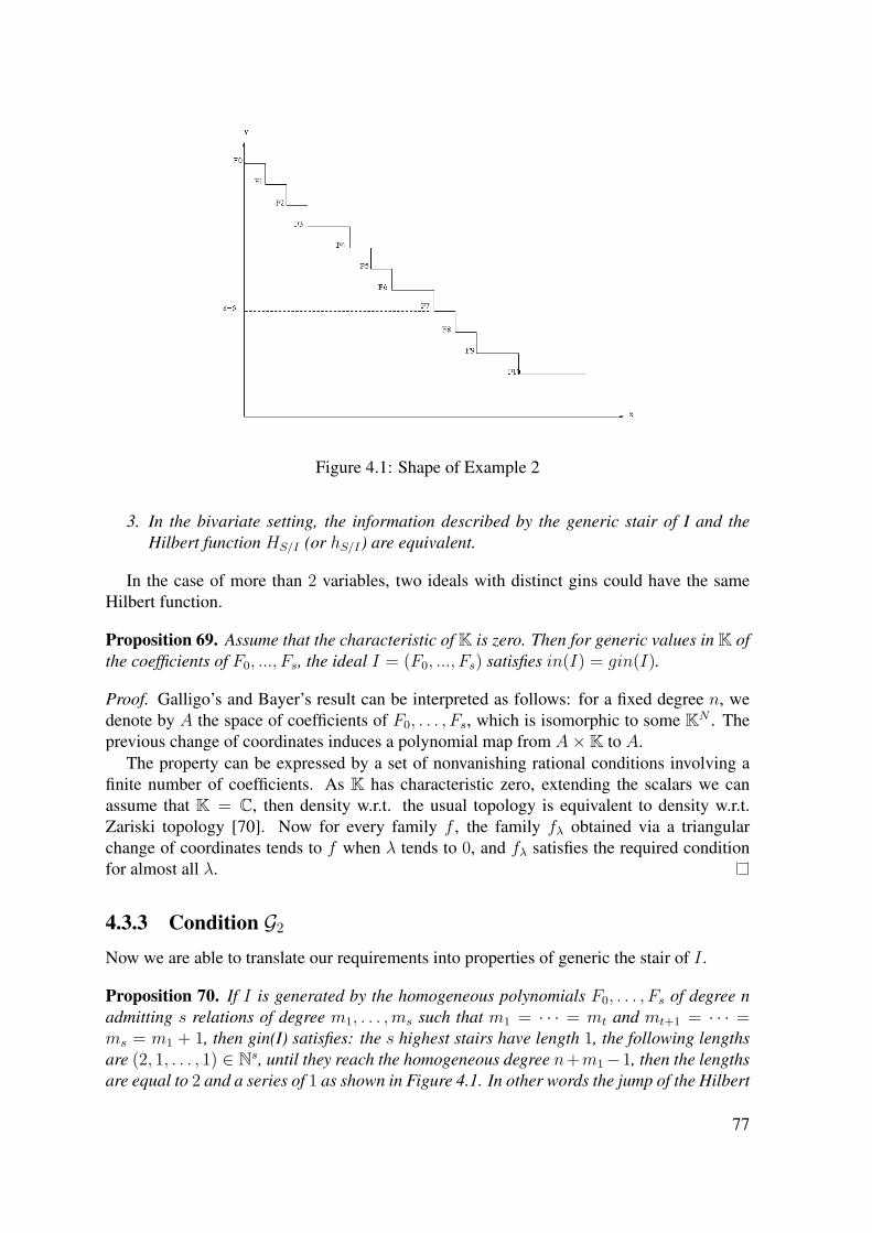
Figure 4.1: Shape of Example 2

3. In the bivariate setting, the information described by the generic stair of I and theHilbert function HS/I (or hS/I) are equivalent.

In the case of more than 2 variables, two ideals with distinct gins could have the sameHilbert function.

Proposition 69. Assume that the characteristic of K is zero. Then for generic values in K ofthe coefficients of F0, ..., Fs, the ideal I = (F0, ..., Fs) satisfies in(I) = gin(I).

Proof. Galligo’s and Bayer’s result can be interpreted as follows: for a fixed degree n, wedenote by A the space of coefficients of F0, . . . , Fs, which is isomorphic to some KN . Theprevious change of coordinates induces a polynomial map from A×K to A.

The property can be expressed by a set of nonvanishing rational conditions involving afinite number of coefficients. As K has characteristic zero, extending the scalars we canassume that K = C, then density w.r.t. the usual topology is equivalent to density w.r.t.Zariski topology [70]. Now for every family f , the family fλ obtained via a triangularchange of coordinates tends to f when λ tends to 0, and fλ satisfies the required conditionfor almost all λ.

4.3.3 Condition G2

Now we are able to translate our requirements into properties of generic the stair of I .

Proposition 70. If I is generated by the homogeneous polynomials F0, . . . , Fs of degree nadmitting s relations of degree m1, . . . ,ms such that m1 = · · · = mt and mt+1 = · · · =ms = m1 + 1, then gin(I) satisfies: the s highest stairs have length 1, the following lengthsare (2, 1, . . . , 1) ∈ Ns, until they reach the homogeneous degree n+m1−1, then the lengthsare equal to 2 and a series of 1 as shown in Figure 4.1. In other words the jump of the Hilbert

77

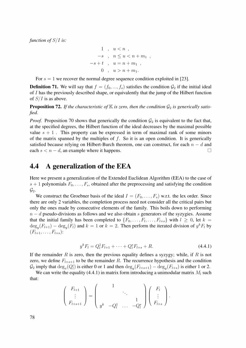
function of S/I is:

1 , u < n ,

−s , n ≤ u < n+m1 ,

−s+ t , u = n+m1 ,

0 , u > n+m1.

For s = 1 we recover the normal degree sequence condition exploited in [23].

Definition 71. We will say that f = (f0, ..., fs) satisfies the condition G2 if the initial idealof I has the previously described shape, or equivalently that the jump of the Hilbert functionof S/I is as above.

Proposition 72. If the characteristic of K is zero, then the condition G2 is generically satis-fied.

Proof. Proposition 70 shows that generically the condition G2 is equivalent to the fact that,at the specified degrees, the Hilbert function of the ideal decreases by the maximal possiblevalue s + 1 . This property can be expressed in term of maximal rank of some minorsof the matrix spanned by the multiples of f . So it is an open condition. It is genericallysatisfied because relying on Hilbert-Burch theorem, one can construct, for each n − d andeach s < n− d, an example where it happens.

4.4 A generalization of the EEAHere we present a generalization of the Extended Euclidean Algorithm (EEA) to the case ofs + 1 polynomials F0, . . . , Fs, obtained after the preprocessing and satisfying the conditionG2.

We construct the Groebner basis of the ideal I = (F0, . . . , Fs) w.r.t. the lex order. Sincethere are only 2 variables, the completion process need not consider all the critical pairs butonly the ones made by consecutive elements of the family. This boils down to performingn− d pseudo-divisions as follows and we also obtain s generators of the syzygies. Assumethat the initial family has been completed to F0, . . . , Fl, . . . , Fl+s with l ≥ 0, let k =degy(Fl+1) − degy(Fl) and k = 1 or k = 2. Then perform the iterated division of ykFl by(Fl+1, . . . , Fl+s):

ykFl = Q1lFl+1 + · · ·+Qs

lFl+s +R. (4.4.1)

If the remainder R is zero, then the previous equality defines a syzygy; while, if R is notzero, we define Fl+s+1 to be the remainder R. The recurrence hypothesis and the conditionG2 imply that degx(Qi

l) is either 0 or 1 and then degy(Fl+s+1)− degy(Fl+s) is either 1 or 2.We can write the equality (4.4.1) in matrix form introducing a unimodular matrixMl such

that: Fl+1

...Fl+s+1

=

1

. . .1

yk −Q1l . . . −Qs

l

Fl...

Fl+s

.

78

Dehomogenizing this construction of a Groebner basis gives rise to the following general-ization of the EEA in normal degree sequence. We set qil(x) = Qi

l(x, 1), fl(x) = Fl(x, 1)and Nl the matrix corresponding to Ml.

We assume that the preprocessing has already been performed.

Algorithm 6: GEEA (Generalized Extended Euclidean Algorithm)Input: Polynomials f0, . . . , fs of degrees n0 = n, . . . , n− s, satisfying the condition

G2.Output: Output: A warning saying that the condition is not satisfied, or a sequence of

remainders and relations expressing these reminders as combinations of theinputs.

1. Initialization: N = Is+1, a = 0, J = 0.

2. For l from 0 to n− s while a = 0 perform a multiple division

fl = q1l fl+1 + · · ·+ qsl fl+s + r.

• If r = 0, then a := 1, J := l + s and update N multiplying by the unimodularmatrix Nl.

• If deg(r) 6= deg(fl+s)− 1, then send a warning and stop.

• If deg(r) = deg(fl+s)− 1, then fl+s+1 := r and update N multiplying by Nl.

3. If a = 1, for l from J − s+ 1 to J − 1, perform a multiple divisionfl = q1

l fl+1 + · · ·+ qJl fJ + r.

• If r = 0, then update N multiplying by the unimodular matrix Nl.

• If r 6= 0, then send a warning and stop.

We have N

f0...fs

=

fJ−s+1

...fJ0

.

4. Invert the unimodular matrix N to get the GCD as a combination of (f0, ..., fs) andalso s generators of the syzygies.

4.5 AlgorithmFor a pair (n, d) of positive integers, the restriction on the degrees e of the perturbationsappearing in (1) is described by the following formula:

e < min(d− bn− d

sc, n− d

). (4.5.1)

79

Now, we describe our algorithm to find «small» degree perturbations for the polynomialsf0, . . . , fs to achieve a «large» degree GCD under the condition G2.

Algorithm 7: Construction of the set U defined in (4.1.1)Input: Univariate coprime polynomials f0, . . . , fs of degrees n . . . , n− s, satisfying

the condition G2. Integers d, e with d > 0 and e as in (4.5.1).Output: The set U .

1. Let F0, . . . , Fs be the homogenized polynomials to degree n of f0, . . . , fsrespectively.

2. Apply the GEEA algorithm to F0, . . . , Fs.

3. Check the expected pattern of degrees. If not, return U = ∅ or a warning.

4. We have for 1 ≤ v ≤ s

Fn−d+v = w0vF0 + · · ·+ wsvFs

where the wjv are some of the entries of the matrix P , the inverse of Mn−d+s. Denotethe corresponding s× s-minors by D0, . . . , Ds, then form

H0 := F0 quoD0 , . . . , Hs := Fs quoDs.

If H0, . . . , Hs are not associates, return U = ∅.Else, compute U0 := −F0 remD0 , . . . , Us := −Fs remDs.

5. Dehomogenize Ui and check if deg ui ≤ e for i = 0 . . . s, then returnU = (u0, . . . , us), else return U = ∅.

Remark 73. Since Fi = HiDi − Ui, i = 0 . . . s, the matrix P gives s syzygies betweenF0 + u0, . . . , Fs + us, then we deduce from Cramer’s rule that the polynomials H0, . . . , Hs

are associates.

Notation: As usual in complexity analysis, O means that we neglect log factors, see [71].For polynomials of degrees at most n, multiplication and Euclidean division require O(n)field operations.

We recall that multiplication or inversion of invertible matrices of order s require O(sω)field operations, ω < 3.

Theorem 74. If f0, . . . , fs satisfy the specification of GEEA, then the set U defined by(4.1.1) contains at most one element. When U is not empty, Algorithm 7 computes it with atmost O(s3n2) field operations.

Proof. We first have to check that any (u0, ..., us) returned by the previous algorithm isactually in U . If we denote by di (resp. hi) the polynomial obtained dehomogenizing Di

80

(resp. Hi), we have

gcd(f0 + u0, . . . , fs + us) = gcd(d0h0, . . . , dshs)= h gcd(d0, . . . , ds) = h,

gcd(d0, ..., ds) = 1 since the matrix for passing from f0, ..., fs to fn−d, ..., fn−d+s is unimod-ular and the computation of its determinant along the first line provides a Bezout relationbetween its minors d0, ..., ds. Then deg h = deg f0−deg d0 = d and indeed (u0, ..., us) ∈ U .

To show the correctness of the algorithm we show that U has at most one element, and ifU 6= ∅, then Algorithm 7 returns this element.

Assume that U 6= ∅. Let (u0, ..., us) in U and h = gcd(f0+u0, ..., fs+us), with deg h = d.For simplicity we assumed in the beginning that d < n − s (Indeed, the special cases

d = n, . . . , d = n− s can be treated directly along the same ideas).Thus, from the condition on the degrees of ui there exist uniquely determined d0, ..., ds in

K[x] such that fi = dih − ui for i = 0 . . . s. Let fi = fi + ui for i = 0 . . . s and executethe GEEA algorithm with the homogenized polynomials F0, ..., Fs of f0, ..., fs respectively.Because of the restriction on the degrees of the perturbation, the GEEA produces the samestairs up to degree n + m1, hence the sequence m = (m1, . . . ,ms) of the degrees of theminimal syzygies of the generated ideal takes the generic value, and we obtain a unimodularmatrix N such that

N

F0

F1...Fs

=

yβH

0...0

.

This implies the uniqueness property of D0, ..., Ds (up to a constant).

The cost for computing the n − d generalized polynomial divisions and multiplying theinverses of the unimodular matrices in the GEEA scheme is bounded by O(s3n2). All otheroperations are not more expensive.

4.6 ExamplesIn the first example, we illustrate the different steps of our algorithm. In the second example,we see how we can loose uniqueness when we relax the bound on the degree of the pertur-bation: the GEEA scheme allows to compute an approximate GCD of degree 2, but failsto detect other approximate GCDs of degree 2. This shows that our recognition approachrequires strong bounds on the degree of the perturbation.

Example 75.

f0 = x14 − 3x13 + x11 + 2x9 − 3x8 − 9x7 + x6 + 3x5 + 4x3 + x2 − 2x− 2,f1 = x12 + x9 + 2x8 + 10x7 + 3x6 + 2x4 + 7x3 + 22x2 + 23x,f2 = x11 + x10 − x8 + 2x7 + 5x6 + 5x5 + 3x4 + x2 + 11x+ 9,f3 = x10 − x9 + x8 + x7 − 2x6 + 2x5 + x4 + 4x2 − x− 5.

81

These polynomials are coprime, and we aim to find a perturbation (u0, u1, u2, u3) of(f0, f1, f2, f3) such that deg(gcd(f0 + u0, f1 + u1, f2 + u2, f3 + u3)) = 6.

We first perform the preprocessing to get a sequence with consecutive degrees. It amountsto replace f0 by f0 := f0 − x2f1, that is

f0 = −3x13 − 2x10 − 8x9 − 6x8 − 9x7 − x6 − 4x5 − 22x4 − 19x3 + x2 − 2x− 2.

The unimodular transition matrix V is the identity plus a matrix having only one nonzeroentry, namely −x2 on the first line.

Therefore, the condition G1 will be satisfied if the degrees of u0, u1, u2, u3 are bounded by7, but the degree of u1 should be bounded by 5. Here, the simplicity of V allows us to makea distinction between the degrees of the different ui. Then we solve the problem replac-ing the input sequence of polynomials by (f0, f1, f2, f3) and we aim to find a perturbation(v0, v1, v2, v3) such that deg(gcd(f0+v0, f1+v1, f2+v2, f3+v3)) = 6, with v0 = −x2u1+u0,v1 = u1, v2 = u2, v3 = u3. Then the new data are s = 3, n = 13, d = 6, and e < 4.

Following Theorem 74 to achieve uniqueness, we impose that the degrees of all vi arebounded by 3. However due to the special form of V this imposes further that deg(v1) ≤3− 2 = 1.

Presenting only the dehomogenized expressions, we successively compute the polynomi-als fj for j = 4, . . . , 10. We get

f4 = −x9 + 23x8 − x7 + x6 − 2x4 + 47x3 + 66x2 − x+ 3,

f5 = 67x8 + 3x7 + 8x6 − 2x4 + 147x3 + 206x2 + 23x+ 23,

f6 = 1067x

7 + 38467 x

6 − 2967x

4 + 8867x

3 + 10667 x

2 + 70267 x+ 1037

67 ,

f7 = 79885 x6 − 523

5 x4 + 1826

5 x3 + 17575 x2 + 14004

5 x+ 215545 ,

f8 = − 267x

5 + 15719535196x

4 − 11709267598x

3 − 3543535196x

2 + 1434133799x−

2841133799 ,

f9 = −222290791159760 x4 − 12672447

15976 x3 + 158546991159760 x2 + 5305998

9985 x+ 6598837988 ,

f10 = 3886987513251185362x

3 − 1226832513251185362x

2 − 993572513251185362x+ 12166625

13251185362 .

Figure 4.1 shows the stairs of this example.We look for perturbations such that the perturbed f8, f9, f10 vanish. So we express them

as combinations of f0, f1, f2, f3 and we get a matrix with 3 rows and 4 columns. Its 3 × 3-minors D0, D1, D2, D3 are polynomials of degrees 7,6,5,4 respectively.

Then (up to a sign) the polynomials Hi = fi quoDi, i = 0 . . . 3, are equal to H =−7988

5 x6 − 159765 x− 23964

5 , the GCD candidate.The remainders rem(f0, D0) = 4x3 +x2 +1, rem(f1, D1) = −x, rem(f2, D2) = 2x3−x

and rem(f3, D3) = x3 − x2 + 1 provide the perturbation. Theorem 74 asserts that the onlysolution is U = (−4x3−x2−1, x,−2x3 +x,−x3 +x2−1), which has degree (3, 1, 3, 3).

82

Remark 76. In this example if we relax the degree bound on the perturbation to (3, 3, 3, 3)we loose uniqueness. We also observe this behavior on the following example. To be moreillustrative we present the homogenized version.

Example 77.

f0 = (x2 − 2x+ 3)(x4 + x3 + x2 + 2x+ 3)− 7 = x6 − x5 + 2x4 + 4x3 + 4x2 + 2

f1 = (x2 − 2x+ 3)(x3 + 2x2 + x− 1) + 4 = x5 + 3x2 + 5x+ 1f2 = (x2 − 2x+ 3)(x2 + 2x+ 2) = x4 + x2 + 2x+ 6.

These polynomials are coprime. Here n = 6, d = 2, then Theorem 74 applies and guar-anties uniqueness if e < 0. With this requirement, the result of Algorithm 7 is U = ∅.

However, as we constructed our example by a perturbation, we do know that with e =0 there is a solution and we want to see if our algorithm detects it although the requiredcondition on the degree is not satisfied. It will not!

Let us see what happens if we just run the process. We look for a perturbation (u0, u1, u2)of (f0, f1, f2) such that deg(gcd(f0 + u0, f1 + u1, f2 + u2)) = 2.

The corresponding homogenized polynomials to degree 6 are

F0 = x6 − yx5 + 2y2x4 + 4y3x3 + 4y4x2 + 2y6

F1 = yx5 + 3y4x2 + 5y5x+ y6

F2 = y2x4 + y4x2 + 2y5x+ 6y6.

Applying the GEEA, we obtain

F3 = y4x3 − 9y7 = yF0 + (y − x)F1 − 2yF2

F4 = y5x2 − y6x− 8y7 = yF1 − xF2 + F3

F5 = 12y7x+ 14y8 = y2F2 − xF3 − yF4

F6 = −232 y

8 = yF3 − (y + x)F4 −34F5.

Figure 4.2 is a picture of the stairs for this example.

Figure 4.2: Shape of Example 3

83

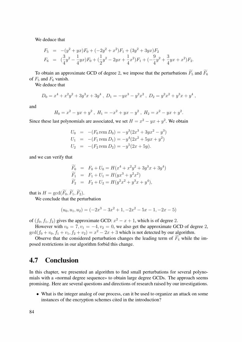
We deduce that

F5 = −(y2 + yx)F0 + (−2y2 + x2)F1 + (3y2 + 3yx)F2

F6 = (34y2 − 1

4yx)F0 + (12y2 − 2yx+ 1

4x2)F1 + (−9

4y2 + 3

4yx+ x2)F2.

To obtain an approximate GCD of degree 2, we impose that the perturbations F5 and F6of F5 and F6 vanish.

We deduce that

D0 = x4 + x2y2 + 3y3x+ 3y4 , D1 = −yx3 − y2x2 , D2 = y2x2 + y3x+ y4 ,

andH0 = x2 − yx+ y2 , H1 = −x2 + yx− y2 , H2 = x2 − yx+ y2.

Since these last polynomials are associated, we set H = x2 − yx+ y2. We obtain

U0 = −(F0 remD0) = −y3(2x3 + 3yx2 − y3)U1 = −(F1 remD1) = −y4(2x2 + 5yx+ y2)U2 = −(F2 remD2) = −y5(2x+ 5y).

and we can verify that

F0 = F0 + U0 = H(x4 + x2y2 + 3y3x+ 3y4)F1 = F1 + U1 = H(yx3 + y2x2)F2 = F2 + U2 = H(y2x2 + y3x+ y4),

that is H = gcd(F0, F1, F2).We conclude that the perturbation

(u0, u1, u2) = (−2x3 − 3x2 + 1,−2x2 − 5x− 1,−2x− 5)

of (f0, f1, f2) gives the approximate GCD: x2 − x+ 1, which is of degree 2.However with v0 = 7, v1 = −4, v2 = 0, we also get the approximate GCD of degree 2,

gcd(f0 + v0, f1 + v1, f2 + v2) = x2 − 2x+ 3 which is not detected by our algorithm.Observe that the considered perturbation changes the leading term of F4 while the im-

posed restrictions in our algorithm forbid this change.

4.7 ConclusionIn this chapter, we presented an algorithm to find small perturbations for several polyno-mials with a «normal degree sequence» to obtain large degree GCDs. The approach seemspromising. Here are several questions and directions of research raised by our investigations.

• What is the integer analog of our process, can it be used to organize an attack on someinstances of the encryption schemes cited in the introduction?

84

• Generalize [72] and describe the stratification (i.e the incidence relations between thestrata) of the classifying space of s+1 polynomials defined by the sequences of degreesof the minimal syzygies.

• Describe what happens when these sequences are not generic.

• See if the degree restrictions can be weakened.

85

86

Appendix A

Implementation and example

In this appendix we show how to compute a matrix representation, µ-basis of a set of poly-nomial, generalized eigenvalues of a univariate polynomial matrix, intersection points ofcurve/curve and curve/surface, singular points of a parameterized plane curve by using thecomputer algebra system Mathemagix which are developing at INRIA Sophia Antipolis inthe project GALAAD [24] and also by using the Maple. All these programs are included inthe current distribution of Mathemagix, in the shape module mmx/shape/mmx /matrixrepre-sentation or at http://www-sop.inria.fr/members/Luu.Ba_Thang/. This work has been doneduring this thesis in parallel of the theoretical developvements. Almost algorithms are refer-ences in [4, 13, 25, 43, 53].

A.1 µ-basis of a set polynomialsIn this section, we introduce a function to compute µ-basis of a set of polynomials f :=(f0, f1, . . . , fn) with gcd(f0, f1, . . . , fn) = 1 which is defined in the first chapter.

• mubase f.

• mubase_homogeneous(f, var)

Example 78. Compute µ-basis of the set polynomials f := [x4 − 492 x

2 + 1152 x − 33, x4 −

25x2 + 61x− 36, x3 − 132 x

2 + 272 x− 8, 1].

• include "mubase.mmx";

• R:=QQ[’x];

• f:=[R << “x4 − 492 x

2 + 1152 x − 33“, R << “x4 − 25x2 + 61x − 36“, R << “x3 −

132 x

2 + 272 x− 8“, R << “1“];

• mubase f

[[−1, 1, 0, 12x2 − 7

2x+ 3], [−1517 , 1, −2

17 x−1317 ,−1517 x+ 13

17],

[136481x−

315813949 ,

−136481 x+ 3842

13949 ,−68413949x−

641813949 ,

12741073x−

1724613949]]

87

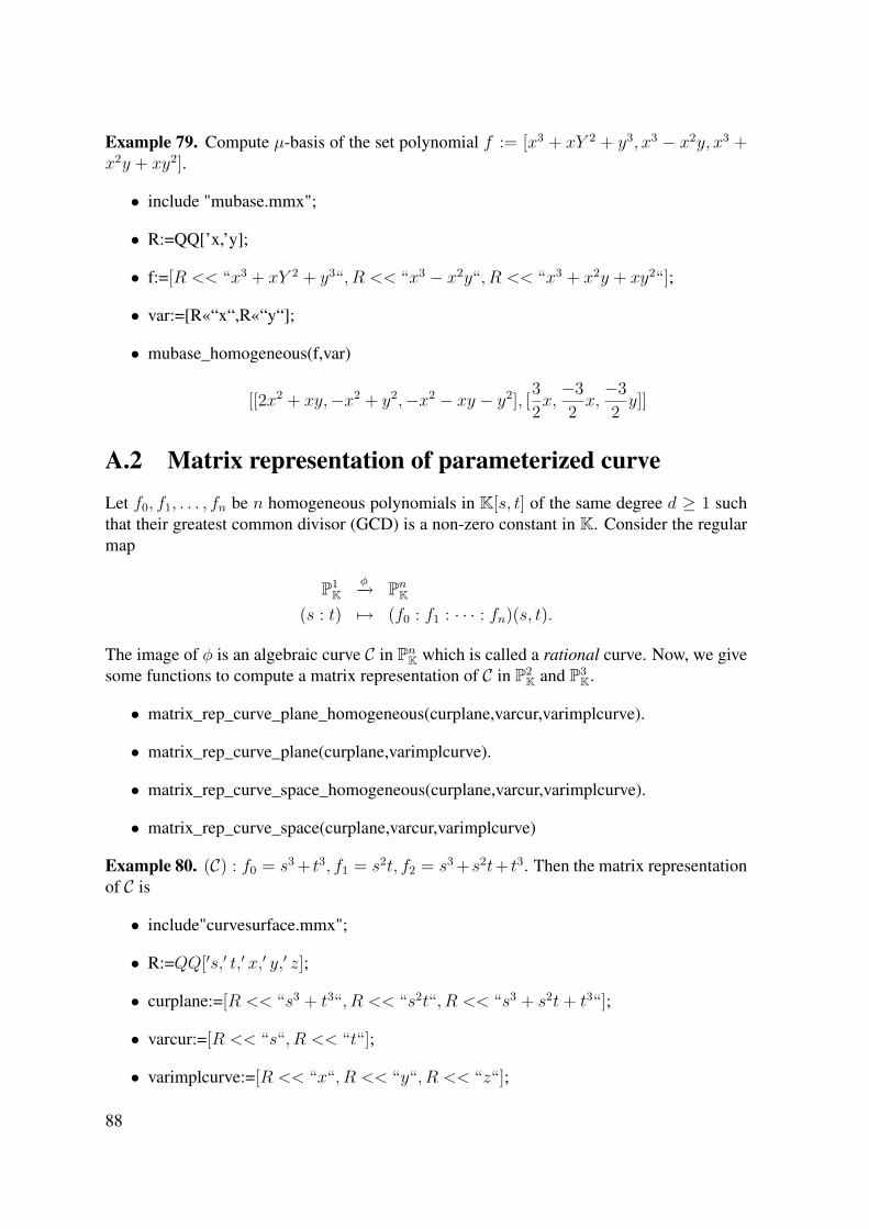
Example 79. Compute µ-basis of the set polynomial f := [x3 + xY 2 + y3, x3 − x2y, x3 +x2y + xy2].

• include "mubase.mmx";

• R:=QQ[’x,’y];

• f:=[R << “x3 + xY 2 + y3“, R << “x3 − x2y“, R << “x3 + x2y + xy2“];

• var:=[R«“x“,R«“y“];

• mubase_homogeneous(f,var)

[[2x2 + xy,−x2 + y2,−x2 − xy − y2], [32x,−32 x,

−32 y]]

A.2 Matrix representation of parameterized curveLet f0, f1, . . . , fn be n homogeneous polynomials in K[s, t] of the same degree d ≥ 1 suchthat their greatest common divisor (GCD) is a non-zero constant in K. Consider the regularmap

P1K

φ−→ PnK(s : t) 7→ (f0 : f1 : · · · : fn)(s, t).

The image of φ is an algebraic curve C in PnK which is called a rational curve. Now, we givesome functions to compute a matrix representation of C in P2

K and P3K.

• matrix_rep_curve_plane_homogeneous(curplane,varcur,varimplcurve).

• matrix_rep_curve_plane(curplane,varimplcurve).

• matrix_rep_curve_space_homogeneous(curplane,varcur,varimplcurve).

• matrix_rep_curve_space(curplane,varcur,varimplcurve)

Example 80. (C) : f0 = s3 + t3, f1 = s2t, f2 = s3 +s2t+ t3. Then the matrix representationof C is

• include"curvesurface.mmx";

• R:=QQ[′s,′ t,′ x,′ y,′ z];

• curplane:=[R << “s3 + t3“, R << “s2t“, R << “s3 + s2t+ t3“];

• varcur:=[R << “s“, R << “t“];

• varimplcurve:=[R << “x“, R << “y“, R << “z“];

88

• matrix_rep_curve_plane_homogeneous(curplane,varcur,varimplcurve) x− z y 0x x− z y−y 0 x− z

Example 81. (C) : f0 = 3s2t, , f1 = −3s3 + 3st2, f2 = st2 + t3, f3 = t3. Then the matrixrepresentation of C is

• include"curvesurface.mmx";

• R:=QQ[′s,′ t,′ x,′ y,′ z,′w];

• curplane:=[R << “3s2t“, R << “− 3s3 + 3st2“, R << “st2 + t3“, R << “t3“];

• varcur:=[R << “s“, R << “t“];

• varimplcurve:=[R << “x“, R << “y“, R << “z“, R << “w“];

• matrix_rep_curve_space_homogeneous(curplane,varcur,varimplcurve)(−y −x− y −z + w

−x+ 3w −x+ 3z w

)

A.3 Matrix representation of parameterized surfaceLet f0, f1, f2, f3 be homogeneous polynomials in K[s, t, u] of the same degree d ≥ 1 suchthat their greatest common divisor (GCD) is a non-zero constant in K. Consider a surface Sgiven by parametrization

P2K

φ−→ P3K

(s : t : u) 7→ (f0(s, t, u) : f1(s, t, u) : f2(s, t, u) : f3(s, t, u)).

Now, we give a function to compute a matrix representation of S in P3K.

• matrix_rep_surface(surface,varsur,varimplsur).

Example 82. Stein’s Roman Surface (S) : f0 = s2 + t2 + u2, f1 = st, f2 = su, f3 = tu.Then the matrix representation of S is

• include"curvesurface.mmx";

• R:=QQ[′s,′ t,′ u,′ x,′ y,′ z,′w];

• Stein:=[R << “s2 + t2 + u2“, R << “st“, R << “su“, R << “tu“];

• varsur:=[R << “s“, R << “t“, R << “u“];

• varimplsur:=[R << “x“, R << “y“, R << “z“, R << “w“];

89

• matrix_rep_curve_surface(surface,varsur,varimplsur)

y y z w 0 0 y 0 0−x −x 0 0 w z −x 0 0y y 0 0 0 0 y z w0 0 −x −y 0 −y w 0 y0 z y 0 −y 0 0 −y −xy 0 z 0 0 0 0 0 w

A.4 Polynomial matrix and generalized eigenvaluesSuppose given a polynomial matrixM(t) = (aij(t)) of sizem×n. if d := maxi,jdeg(ai,j(t)then

M(t) = Mdtd +Md−1t

d−1 + . . .+M0

where Mi ∈ Km×n.We construct some functions to compute Md,Md−1, . . . ,M0, generalized companion ma-

trices, regular matrix and generalized eigenvalues of M(t) which are defined in the secondchapter.

• list_coefficients_matrix M(t).

• firstcompanionmatrix M(t).

• secondcompanionmatrix M(t).

• pencilregular(A,B) where A:=firstcompanionmatrix M(t), B:=secondcompanionmatrixM(t).

• generalized_eigenvalues M(t).

Example 83. M :=

3x2 −3x3 + 3xx+ 1 1

2x2 + x x2 + x

• include“pencilregular.mmx“;

• degree M3

• list_coefficients_matrix M

M3 =

0 −30 00 0

,M2 =

3 00 02 1

,M1 =

0 31 01 1

,M0 =

0 01 10 0

• A:=firstcompanionmatrix M;

• B:=secondcompanionmatrix M;

90

• pencilregular(A,B)[[0], [−3]]

• generalized_eigenvalues M[0]

A.5 Parameterized curve/curve intersectionConsider two curves C1, C2 given by parametrization

(C1) : P1K

φ1−→ PnK(s : t) 7→ (f0(s, t) : f1(s, t) : · · · : fn(s, t)).

(C2) : P1K

φ2−→ PnK(s : t) 7→ (g0(s, t) : g1(s, t) : · · · : gn(s, t)).

Hereafter, we give some functions to compute the intersection locus C1 ∩ C2 in the space P2K

and P3K.

• intersection_curve_plane_homogeneous(curve1,varcur1,curve2,varcur2).

• intersection_curve_space_homogeneous(curve1,varcur1,curve2,varcur2).

In the case, the parametrization of C1 and C2 are given the univariate polynomial, we give theother functions to compute the intersection locus C1 ∩ C2.

• intersection_curve_plane(curve1,curve2).

• intersection_curve_space(curve1,curve2).

Example 84. (C1) : f0 = x4 − 492 x

2 + 1152 x − 33, f1 = x4 − 25x2 + 61x − 36, f2 =

x3 − 132 x

2 + 272 x− 8, f3 = 1.

(C2) : g0 = x3−112 x

2+172 x−3, g1 = x3−6x2+12x−6, g2 = x4−51

2 x2+125

2 x−38, g3 = 1.Then C1 ∩ C2 are

• include “curvesurface.mmx“;

• R:=QQ[’x];

• curve1:=[R << “x4 − 492 x

2 + 1152 x − 33“, R << “x4 − 25x2 + 61x − 36“, R <<

“x3 − 132 x

2 + 272 x− 8“, R << “1“];

91

• curve2:=[R << “x3 − 112 x

2 + 172 x − 3“, R << “x3 − 6x2 + 12x − 6“, R <<

“x4 − 512 x

2 + 1252 x− 38“, R << “1“];

• intersection_curve_space(curve1,curve2)

[[1, 1, 0, 1], [0, 2, 1, 1], [0, 3, 1, 1], [−308,−341,−363, 1]

Example 85. (C1) : f0 = x3−3x2y+2xy2+y3, f1 = x2y+2xy2+2y3, f2 = xy2+3y3, f3 =y4.(C2) : g0 = x4 − xy3 + y4, g1 = xy3 + y4, g2 = xy3 + 2y4, g3 = y4. Then C1 ∩ C2 are

• include “curvesurface.mmx“;

• R:=QQ[’x,’y];

• curve1:=[R << “x3 − 3x2y + 2xy2 + y3“, R << “x2y + 2xy2 + 2y3“, R << “xy2 +3y3“, R << “y4“];

• curve2:= [R << “x4−xy3 +y4“, R << “xy3 +y4“, R << “xy3 +2y4“, R << “y4“];

• varcur:=R << “x“, R << “y“];

• intersection_curve_space_homogeneous(curve1,varcur,curve2,varcur)

[[1, 2, 3, 1], [1, 1, 2, 1]].

A.6 Parameterized curve/surface intersectionConsider a curve C given by parametrization

(C) : P1K

φ−→ P3K

(s : t) 7→ (f0(s, t) : f1(s, t) : f2(s, t) : f3(s, t)).

and a surface S by parametrization

(S) : P2K

ψ−→ P3K

(s : t : u) 7→ (g0(s, t, u) : g1(s, t, u) : g2(s, t, u) : g3(s, t, u)).

We give a function to determinate the intersection locus C ∩ S.

• intersection_curve_surface_homogeneous(surface,varsur,curve,varcur).

Example 86. A sphere (S) : f0 = x2 + y2 + z2, f1 = 2xz, f2 = 2xy, f3 = x2 − y2 − z2.A thwisted cubic: (C) : g0 = s3, g1 = s2t, g2 = st2, g3 = t3. Then S ∩ C are

• include “curvesurface.mmx“;

92

• R:=QQ[’s,’t,’x,’y,’z];

• surface:=[R << “x2 + y2 + z2“, R << “2xz“, R << “2xy“, R << “x2 − y2 − z2“];

• curve:=;[R << “s3“, R << “s2t“, R << “st2“, R << “t3“];

• varsur:=[R << “x“, R << “y“, R << “z“;

• varcur:=[R << “s“, R << “t“, ];

• intersection_curve_surface_homogeneous(surface,varsur,curve,varcur)

[[1,−0.73, 0.54,−0.4], [1, 0.73, 0.54, 0.4],

[1, 0.54−1.03i,−0.77−1.11i,−1.56+0.19i], [1, 0.54+1.03i,−0.77+1.11i,−1.56−0.19i],[1,−0.54−1.03i,−0.77+1.11i, 1.56+0.19i], [1,−0.54+1.03i,−0.77−1.11i, 1.56−0.19i]]

A.7 Singular points of parameterized plane curveConsider a plane curve C given by parametrization

(C) : P1K

φ−→ P2K

(s : t) 7→ (f0(s, t) : f1(s, t) : f2(s, t)).

We given a function to compute the singular points of C with its multiplicity.

• singular_point_plane(curve,varcur,int) where «int» is multiplicity of a points on C.

Example 87. (C) : f0 = t5−2∗t3+2, f1 = t4+3, f2 = 1. Then P (2, 7, 1) is of multiplicity2 and Q(2, 3, 1) is of multiplicity 3.

• include “singular_point.mmx“;

• R:=QQ[’t,’x,’y,’z];

• curve:= [R << “t5 − 2 ∗ t3 + 2“, R << “t4 + 3“, R << “1“;

• varcur:= [R << “t“, R << “x“, R << “y“, R << “z“];

• singular_point_plane(curve,varcur,2)

[2, 7, 1], [2 + 8i,−1, 1], [2− 8i,−1, 1]

• singular_point_plane(curve,varcur,3)

[[2, 3, 1]]

• singular_point_plane(curve,varcur,4)[]

93

Example 88. (Chen, F and all) (C) : f0 = t4 − 40 ∗ t3 + 40t+ 1, f1 = t4 + 480t2 + 1, f2 =t4 + 40t3 + 480t2 + 40t+ 1.

• include “singular_point.mmx“;

• R:=QQ[’t,’x,’y,’z];

• curve:= [R << “t4− 40 ∗ t3 + 40t+ 1“, R << “‘t4 + 480t2 + 1‘, R << “t4 + 40t3 +480t2 + 40t+ 1“;

• varcur:= [R << “t“, R << “x“, R << “y“, R << “z“];

• singular_point_plane(curve,varcur,2)

[[2.4488708221968 ∗ 107, 5.0600587305910 ∗ 107, 7.3417921728759 ∗ 107],

[7714.2545820696, 15939.828632115, 8752.0780563547],

[7.9346835678021, 16.395297170358, 23.788432278383],

[0.51773816346332, 1.0697932657153, 0.58739114339276], [1, 1, 1]]

• singular_point_plane(curve,varcur,3)[]

• singular_point_plane(curve,varcur,4)[]

A.8 Solve the equation of univariate polynomialsLet f(x) be an univariate polynomial of the rational coefficients. We give a function to findall roots of f(x).

• solve f(x)

Example 89. Solve the equation x4 + 2x+ 1 = 0.

• include “solvepolynomial.mmx“;

• f:=QQ[′x] << “x4 + 2x+ 1“;

• solve f;

[0.77184450634604+1.1151425080399∗i, 0.77184450634604−1.1151425080399∗i,

−1.0000000000000,−0.54368901269208]

.

94

Conclusion

In this thesis, we have obtained some new results following:

• Introduce a new implicit representation of rational curves of arbitrary dimensions andpropose a implicit representation of rational hypersurfaces.

• Illustrate the advantages of this matrix representation by addressing several importantproblems of Computer Aided Geometric Design (CAGD): The intersection problemcurve/curve, curve/surface and surface/surface, the point-on-curve and inversion prob-lems, the computation of singularities of rational curves.

• Develop a symbolic/numeric algorithm to manipulate these new representations for ex-ample: the algorithm for extracting the regular part of a non square pencil of univariatepolynomial matrices and bivariate polynomial matrices.

• Describes an algorithm which, given a family of generic univariate polynomials f :=(f0, ..., fs), find polynomial perturbations u := (u0, ..., us) with prescribed degree-bounds such that gcd(f1 + u1, ..., fs + us) has at least a given degree, provided thatsuch a perturbation exists in polynomial time under a generic condition generalizingthe normal degree sequence

• Develop the package matrixrepresentation of the computer algebra system Mathemagixand Maple to these matrices representations.

95

96

Bibliography

[1] Laurent Busé and Marc Dohm. Implicitization of bihomogeneous parametrizations ofalgebraic surfaces via linear syzygies. In ISSAC 2007, pages 69–76. ACM, New York,2007.

[2] Laurent Busé, David Cox, and Carlos D’Andrea. Implicitization of surfaces in P3 inthe presence of base points. J. Algebra Appl., 2(2):189–214, 2003.

[3] David Cox, Ronald Goldman, and Ming Zhang. On the validity of implicitizationby moving quadrics of rational surfaces with no base points. J. Symbolic Comput.,29(3):419–440, 2000.

[4] Laurent Busé and Marc Chardin. Implicitizing rational hypersurfaces using approxi-mation complexes. J. Symbolic Comput., 40(4-5):1150–1168, 2005.

[5] Laurent Busé and Jean-Pierre Jouanolou. On the closed image of a rational map andthe implicitization problem. J. Algebra, 265(1):312–357, 2003.

[6] L. Busé, M. Chardin, and with appendix of J. Oesterlé Aron Simis. Elimination andnonlinear equations of rees algebras. Journal of Algebra, 324(3):1314–1333, 2010.

[7] T.W. Sederberg and F. Chen. Implicitization using moving curves and surfaces. InProceedings of SIGGRAPH, volume 29, pages 301–308, 1995.

[8] Dinesh Manocha and John Canny. A new approach for surface intersection. In Pro-ceedings of the first ACM symposium on Solid modeling foundations and CAD/CAMapplications, pages 209–219, Austin, Texas, United States, 1991. ACM.

[9] Nicolás Botbol, Marc Dohm, and Alicia Dickenstein. Matrix representations for toricparametrizations. Computer Aided Geometric Design, 7:757–771, 2009.

[10] Laurent Busé, Marc Chardin, and Jean-Pierre Jouanolou. Torsion of the symmet-ric algebra and implicitization. Proceedings of the American Mathematical Society,137(06):1855–1865., February 2009.

[11] T. Garrity and J. Warren. On computing the intersection of a pair of algebraic surfaces.Comput. Aided Geom. Design, 6 (2):137–153, 1989.

[12] E. Fortuna, P. Gianni, and B. Trager. Generators of the ideal of an algebraic spacecurve. J. Symbolic Comput, 44 (9):1234–1254, 2009.

97

[13] N. Song and R. Goldman. µ-bases for polynomial systems in one variable. Comput.Aided Geom. Design, 26 (2):217–230, 2009.

[14] X. Jia, H. Wang, and R. Goldman. Set-theoretic generators of rational space curves.Journal of Symbolic Computation, 45 (4):414 – 433, 2010.

[15] D. A. Cox, T. W. Sederberg, and F. Chen. The moving line ideal basis of planar rationalcurves. Comput. Aided Geom. Design, 15 (8):803–827, 1998.

[16] D. A. Aruliah, Robert M. Corless, Laureano Gonzalez-Vega, and Azar Shakoori. Ge-ometric applications of the bezout matrix in the lagrange basis. In Proceedings of the2007 international workshop on Symbolic-numeric computation, pages 55–64, London,Ontario, Canada, 2007. ACM.

[17] Laurent Busé, Houssam Khalil, and Bernard Mourrain. Resultant-based methods forplane curves intersection problems. In Computer algebra in scientific computing, vol-ume 3718 of Lecture Notes in Comput. Sci., pages 75–92. Springer, Berlin, 2005.

[18] H. Wang, X. Jia, and R. Goldman. Axial moving planes and singularities of rationalspace curves. Comput. Aided Geom. Design, 26 (3):300–316, 2009.

[19] H.-S. Heo, M. S. Kim, and G. Elber. The intersection of two ruled surfaces. Computer-Aided Design, 31(1):33–50, 1999.

[20] M. Fioravanti, L. Gonzalez-Vega, and I. Necula. Computing the intersection of tworuled surfaces by using a new algebraic approach. Journal of Symbolic Computation,41 (11):1187 – 1205, 2006.

[21] V.N. Kublanovskaya and V.B. Khazanov. Spectral problems for pencils of polynomialmatrices. methods and algorithms. v. Journal of Mathematical Sciences, 79(3):1048–1076, 1996.

[22] V.N. Kublanovskaya. Methods and algorithm of solving spectral problems for polyno-mial matrices and rational matrix. Journal of Mathematical Sciences, 96(3):3085–3287,1999.

[23] J. von zur Gathen, M. Mignotte, and I. E. Shparlinski. Approximate polynomialgcd: Small degree and small height perturbations. Journal of Symbolic Computation,45:879–886, 2010.

[24] The software mathemagix. Available at http://www.mathemagix.org.

[25] L. Busé and T. Luu Ba. Matrix-based implicit representations of algebraic curves andapplications. Computer Aided Geometric Design, 27(9):681–699, 2010.

[26] Amit Khetan and Carlos D’Andrea. Implicitization of rational surfaces using toricvarieties. J. Algebra, 303(2):543–565, 2006.

[27] C. D’Andrea. Resultant and moving surfaces. Journal of Symbolic Computation,31:585–602, 2001.

98

[28] L. Busé and M. Chardin. Implicitizing rational hypersurfaces using approximationcomplexes. Journal of Symbolic Computation, 40:1150–1168, 2005.

[29] A. Simis and W.V. Vasconcelos. The syzygies of the conormal module. Amer. J. Math,103:203–224, 1981.

[30] W.V. Vasconcelos. Arithmetic of Blowup Algebras. In London Mathematical SocietyLecture Note Series vol 195. Cambridge University Press.

[31] W. Bruns and J. Herzog. Cohen-Macaulay rings. Cambridge studies in advancedmathematics 39. Cambridge university press 1993.

[32] M. Dohm. Implicitization of rational ruled surfaces with µ-bases. Journal of SymbolicComputation, 5:479–489, 2009.

[33] D. Eisenbud. Commutative algebra with a view toward algebraic geometry. Vol 150.Springer-Verlag, New York.

[34] Joe Harris. Algebraic Geometry. A first course. Graduate Texts in Mathematics 133.Apringer-Verlag NewYork, Inc 1992.

[35] D. Cox, J. Little, and D. O’Shea. Ideals, varieties, and algorithms. 2nd Edition.Springer-Verlag, New York, Undergraduate Texts in Mathematics.

[36] L. Busé. Elimination theory in codimension one and applications. Notes of lecturesgiven at the CIMPA-UNESCO-IRAN school in Zanjan, Iran, July 9-22, 2005.

[37] J. P. Jouanolou. Idéaux résultants. Adv. in Math, 37 (3):212–238, 1980.

[38] D. G. Northcott. Finite free resolutions. No. 71. Cambridge University Press, cam-bridge Tracts in Mathematics, 1976.

[39] D. R. Grayson and M. E. Stillman. Macaulay2, a software system for research inalgebraic geometry. Available at http://www.math.uiuc.edu/Macaulay2/.

[40] L. Busé and R. Goldman. Division algorithms for Bernstein polynomials. Comput.Aided Geom. Design, 25 (9):850–865, 2008.

[41] Ernst Kunz. Introduction to plane algebraic curves. Translated from the original Ger-man by Richard G. Belshoff, 2005.

[42] J. Zheng and T. W. Sederberg. A direct approach to computing the µ-basis of planarrational curves. J. Symbolic Comput, 31(5):619–629, 2001.

[43] T. Luu Ba, L. Busé, and B. Mourrain. Curve/surface intersection problem by meansof matrix representation. In SNC’09: Proceedings of the International Conferenceon Symbolic Numeric Computation. Kyoto, Japan.ACM, NewYork, USA, pages 71–78,August 2009.

99

[44] F. R. Gantmacher. Théorie des matrices. Tome 2: Questions spéciales et applications.Traduit du Russe par Ch. Sarthou. Collection Universitaire de Mathématiques, No. 19.Dunod, Paris, 1966.

[45] Gene H. Golub and Charles F. Van Loan. Matrix computations. Johns Hopkins Studiesin the Mathematical Sciences. Johns Hopkins University Press, Baltimore, MD, thirdedition, 1996.

[46] F. R. Gantmacher. Théorie des matrices. Tome 1: Théorie générale. Traduit du Russepar Ch. Sarthou. Collection Universitaire de Mathématiques, No. 18. Dunod, Paris,1966.

[47] Paul Van Dooren and Patrick Dewilde. The eigenstructure of an arbitrary polynomialmatrix: computational aspects. Linear Algebra Appl., 50:545–579, 1983.

[48] A. Amiraslani, R.M. Corless, and P. Lancaster. Linearization of matrix polynomialsexpressed in polynomial bases. IMA. J. Number. Anal, 1:141–157, 2009.

[49] P. Van Dooren. The computation of kronecker’s canonical form of a singular pencil.Linear Algebra and its Applications, 27:103–140, 1979.

[50] Th. Beelen and P. Van Dooren. An improved algorithm for the computation of Kro-necker’s canonical form of a singular pencil. Linear Algebra Appl., 105:9–65, 1988.

[51] B. Mourrain. Computing isolated polynomial roots by matrix methods. J. of SymbolicComputation, Special Issue on Symbolic-Numeric Algebra for Polynomials, 26(6):715–738, Dec. 1998.

[52] B. Mourrain. Bezoutian and quotient ring structure. J. of Symbolic Computation,39(3):397–415, 2005.

[53] F. Chen, W. Wang, and Y. Liu. Computing singular points of plane rational curves. J.Symbolic Comput, 43(2):92–117, 2008.

[54] L. Busé and C. D’Andrea. Singular factors of rational plane curves. Preprint,arXiv:0912.2723, 2009.

[55] R. Rubio, J.M. Serradilla, and M.P.Vélez. Detecting real singularities of a space curvefrom a real rational parametrization. Journal of Symbolic Computation, 44:490–498,2009.

[56] G. W. Stewart. On the sensitivity of the eigenvalue problems ax = λbx. SIAM J.Numer. Anal. 9, 4:669–689, 1972.

[57] A. Mantzaflaris and B. Mourrain. A subdivision approach to planar semi -algebraicsets. In Proceedings of the 6th international Conference GMP, Castro Urdiales, Spain,pages 104–123, June 2010.

100

[58] M. Elkadi, A. Galligo, and T. Luu Ba. Approximate gcd of several univariate polyno-mials, small degree perturbations. Journal of Symbolic Computation, issue in honourof Joachim von zur Gathen, 2011.

[59] N. Howgrave-Graham. Approximate integer common divisors. In Cryptography andlattices (Providence, RI, 2001). volume 2146 of Lecture Notes in Comput. Sci., pages51–66. Springer, Berlin, 2001.

[60] M. Van Dijk, C. Gentry, S. Halavi, and V. Vaikuntanathan. Fully homomorphic encryp-tion over the integers. In Advances in cryptology – EUROCRYPT 2010, volume 6110of Lecture Notes in Computer Science, pages 24–43. Springer, Berlin, 2010.

[61] D. A. Bini and P. Boito. Structured matrix-based methods for polynomial ε-gcd: anal-ysis and comparisons. In In ISSAC, ACM, New York, pages 9–16, 2007.

[62] I. Z. Emiris, A. Galligo, and H. Lombardi. Certified approximate univariate GCDs. J.Pure Appl. Algebra, 117/118:229–251, 1997.

[63] E. Kaltofen, Z. Yang, and L. Zhi. Approximate greatest common divisors of severalpolynomials with linearly constrained coefficients and singular polynomials. In In IS-SAC 2006, ACM, New York, pages 169–176, 2006.

[64] N. K. Karmarkar and Y. N. Lakshman. On approximate GCDs of univariate polynomi-als. J. Symbolic Comput, 26(6):653–666, 1998.

[65] V. Y. Pan. Computation of approximate polynomial GCDs and an extension. Inform.and Comput, 167(2):71–85, 2001.

[66] D. Rupprecht. An algorithm for computing certified approximate GCD of n univariatepolynomials. J. Pure Appl. Algebra, 139(1-3):255–284, 1999.

[67] T. Sasaki and M.-T. Noda. Approximate square-free decomposition and root-finding ofill-conditioned algebraic equations. J. Inform. Process, 12(2):159–168, 1989.

[68] A. Galligo. À propos du théorème de-préparation de Weierstrass. In Fonctions deplusieurs variables complexes (Sém. François Norguet, octobre 1970–décembre 1973;à la mémoire d’André Martineau). Pages 543–579. Lecture Notes in Math., Vol. 409.Springer, Berlin, 1974.

[69] D. Bayer. The division algorithm and the Hilbert scheme. PhD thesis, Harvard Univer-sity. 1982.

[70] D. Mumford. Algebraic Geometry I: Complex Projective Varieties, volume 221 ofGrundlehren der Mathematischen Wissenschaften [Fundamental Principles of Mathe-matical Sciences]. Springer-Verlag, Berlin, 1981.

[71] J. von zur Gathen and J. Gerhard. Modern computer algebra. second edition. Cam-bridge University Press, Cambridge, 2003.

[72] C. D’Andrea. On the structure of µ-classes. Comm. Algebra, 32(1):159–165, 2004.

Répresentation Matricielle Implicite de Courbes et Surfacesalgébriques et Applications

Résumé. Dans cette thèse, nous introduisons et étudions une nouvelle représentationimplicite des hypersurfaces rationelles et des courbes rationnelles plongées dans un espaceprojectif de dimension arbitraire. Nous illustrons les avantages de cette représentation ma-tricielle en abordant plusieurs problèmes importants intervenant en conception géométriqueassistée par ordinateur: les problèmes d’intersection entre deux courbes, entre une courbeet une surface ou bien encore entre deux surfaces, le problème d’appartenance d’un pointà une courbe ou une surface, le problème du calcul de la pré-image d’un point donné parune paramétrisation et enfin le problème du calcul des singularités d’une courbe rationnelle.L’approche développée dans ce travail de thèse est basée sur la combinaison de méthodessymboliques et numériques. En effet, un première étape symbolique consiste à transformerle problème considérer en un pinceau de matrices. La deuxième étape consiste alors à cal-culer les valeurs propres généralisées de ce pinceau à l’aide de méthodes numériques. Pourcela, un algorithme d’extraction de la partie régulière d’un pinceau univarié, respectivementbivarié, de matrices non carrées est présenté. Une implémentation de ces travaux dans lessystèmes de calcul formel Mathemagix et Maple est présentée en appendice. Le dernierchapitre est conscré à un algorithme qui, étant donné un ensemble de polynômes univariésf1, ..., fs construit un ensemble de polynômes u1, ..., us dont les degrés sont prescrits, telsque le degré du pgcd(f1 + u1, ..., fs + us) est supérieur ou égal à un entier donné sous deshypothèses de généricité.

Mots-clés: µ-base, l’élimination, représentations matricielles, problèmes d’intersection,singularités, implicitation, pinceau de matrices, formes de Kronecker, idéal initial générique,PGCD de polynômes, suite normale des degrés, bases de Gröbner.

Matrix-based implicit representations of algebraic curves andsurfaces and applications

Abstract. In this thesis, we introduce and study a new implicit representation of rationalcurves of arbitrary dimensions and propose an implicit representation of rational hypersur-faces. Then, we illustrate the advantages of this matrix representation by addressing sev-eral important problems of Computer Aided Geometric Design (CAGD): The curve/curve,curve/surface and surface/surface intersection problems, the point-on-curve and inversionproblems, the computation of singularities of rational curves. We also develop some sym-bolic/numeric algorithms to manipulate these new representations for example: the algorithmfor extracting the regular part of a non square pencil of univariate polynomial matrices andbivariate polynomial matrices. In the appendix of this thesis work we present an implemen-tation of these methods in the computer algebra systems Mathemagix and Maple. In thelast chapter, we describe an algorithm which, given a set of univariate polynomials f1, ..., fsreturns a set of polynomials u1, ..., us with prescribed degree-bounds such that the degreeof gcd(f1 + u1, ..., fs + us) is bounded below by a given degree assuming some genericityhypothesis.

Keywords: µ-basis, elimination, matrix representations, intersection problems, singulari-ties, implicitation, pencils matrices, Kronecker form, generic initial ideal, GCD of univariatepolynomials, normal degree sequence, Gröbner basis.