Matrix Algebra and Vector Spaces forEconometrics

Roberto Casarin∗

University of VeniceGiacomo Pasini

University of Venice

Yuri PettinicchiSAFE, University of Frankfurt

This version: October 25, 2017

Abstract

This document is the result of a reorganization of lecture notes usedby the authors while teaching and TAing the first course of Economet-rics at the PhD program at the School for advanced Studies in Eco-nomics at the University of Venice. It collects a series of results inMatrix and Tensor Algebra, Matrix and Tensor Calculus and VectorSpaces analysis useful as a background for a course in EconometricTheory at the P.h.D. level. Most of the material is taken from Ap-pendix A of Mardia et al. (1979) and chapters 4, 5 of Noble and Daniel(1988), Magnus and Neudecker (1999) and Kolda and Bader (2009).

1 Vector, Matrix and Tensor Algebra

1.1 Basic definitions

Definition 1 (Matrix) A matrix A is a rectangular array of numbers. IfA has n rows and p columns, we say it is of order n× p

An×p =

a11 . . . a1p...

...an1 . . . anp

= (aij)

Definition 2 (Column vector) A matrix with column–order 1 is calledcolumn vector

∗Department of Economics, University of Venice, E-mail: r.casarin@unive.it.

1

a =

a1...an

Row–vectors are column vector transposed:

a′ =(a1 . . . an

)A matrix can be written in terms of its column (row) vectors:

A = (a(1), . . . ,a(p)) =

a′1...a′n

Notation: we write the j–th column of matrix A as a(j), the i–th row as

ai (if written as a column vector), the ij–th element as (aij).

Definition 3 (Inner Product (or Dot Product or Scalar Product))Let a and b n-dimensional vectors, the inner product is defined as

< a, b >=n∑

i=1

aibi

It is also denoted with a · b.

Definition 4 (Outer Product) Let a and b n- andm-dimensional vectorsrespectively, the outer product a∨ b gives a (n×m) - matrix C with (i, j)-thelement cij = aibj with i = 1, . . . , n and j = 1, . . . ,m.

Theorem 1 The outer product has the following properties

1. u ∨ v 6= v ∨ u

2. w ∨ (αu + βv) = αw ∨ u + βw ∨ v

3. (αu + βv) ∨w = αu ∨w + βv ∨w

4. w · (u ∨ v) = (w · u)v

Note that the definition of matrix and inner product can be extended tothe general notion of tensor and tensor inner products.

Definition 5 (Tensor) A (I1× I2× · · · × IN )-dimensional tensor A is de-fined by a N -dimensional array of with scalar components ai1i2...iN , ij =1, . . . , Ij, j = 1, . . . , N . The order of this tensor is N .

2

Figure 1: A third-order tensor A ∈ RI1×I2×I3

Note that a matrix is a special case of tensor with N = 2. See Figure 1.1for a third-order tensor. A vector is a first-order tensor and a scalar is azeroth-order tensor.

A fiber of a given tensor A is a higher-order analogue of matrix rowsand columns and it is a 1-dimensional array obtained by fixing every indexbut one of the tensor A. The n-mode fiber a(n) is a column vector withi-th element ai1i2...in−1iin+1...iN , i = 1, . . . , In. See Figure 2 for an example offibers of a tensor of the order three.

A slice is a two dimensional array obtained by fixing all but two indices.The (m,n)-mode sliceA(m,n) has (i, j)-the element ai1i2...im−1iim+1...in1−1jin+1...iN

with i = 1, . . . , Im and j = 1, . . . , In. See Figure 3 for an example of slicesof a third-order tensor.

Definition 6 (Inner Product for Tensors) Let A,B ∈ RI1×···×IN twoN -th order tensors, then the inner product is defined as

< A,B >=

I1∑i1=1

· · ·IN∑

iN=1

ai1...iN bi1...iN

It is also denoted with A ·B.

Definition 7 (Partitioned Matrix) A matrix written in terms of its sub–matrices is called a partitioned matrix.

An example of partitioned matrix is:

A(n× p) =

(A11(r × s) A12(r × (p− s))

A21((n− r)× s) A22((n− r)× (p− s))

)

3

(a) (b) (c)

Figure 2: Fibers of the third order tensor A ∈ RI1×I2×I3 . (a) Mode-1(columns) fibers a:i2i3 . (b) Mode-2 (rows) fibers ai1:i3 . (c) Mode-3 (tubes)fibers a11i2:.

(a) (b) (c)

Figure 3: Slices of the third order tensor A ∈ RI1×I2×I3 . (a) Horizontal slicesAi1::. (b) Lateral slices A:i2:. (c) Frontal slices A::i3 .

Definition 8 (Square Matrix) A n × m matrix B is a square matrix ifn = m.

Definition 9 (Diagonal Matrix) Given a n–dimensional vector a, a n×ndiagonal matrix B = diag(a) is a matrix with bii = ai; bij = 0 ∀i 6= j:

B = diag(a) =

a1 . . . 0... ai

...0 . . . an

Given a matrix An×p, B = diag(A) is a matrix with bii = aii; bij = 0

∀i 6= j.

Definition 10 (Cubical Tensor) A N -th order tensor A ∈ RI1×···×IN , isa cubical tensor if I1 = I2 = · · · = IN .

Definition 11 (Diagonal Tensor) A N -th order cubical tensor A ∈ RI×···×I ,

4

Table 1: common types of matricesName Definition NotationScalar p = n = 1 aColumn vector p = 1 aUnit vector p = 1; ai = 1 1 or 1n

Square p = qSymmetric aij = ajiUnit matrix aij = 1; p = n Jp = 11′

(Upper) Triangular aij = 0 ∀j > iNull matrix aij = 0 ∀i, j 0

is diagonal if its element ai1...iN = 0 for all N -nuples (i1, i2, . . . , iN ) such thatil 6= ik for some k and l.

1.2 Matrix and tensor operations

Table 2: Basic matrix operationsOperation Restrictions DefinitionsAddition A,B same order A + B = (aij + bij)Subtraction A,B same order A−B = (aij − bij)Scalar multiplication cA = (caij)Inner product a, b same order a′b =

∑i aibi

Definition 12 (Matrix Product) If A,B are conformable, i.e. the num-ber of columns of A equals the number of rows of B, then AB is the matrixwith at each entry abij has the inner product of the i–th row vector of A andthe j–th column vector of B:

AB = (a′ib(j))

Remark: in general AB 6= BA

Definition 13 (Tensor Matrix Product) The n-mode matrix product ofa tensor A ∈ RI1×I2×···×IN with a matrix B ∈ RJ×In is the tensor C =A×n B of size I1 × In−1 × J × In+1 × IN with element

ci1i2···in−1jin+1···iN =

In∑in=1

ai1i2···iN bjin

5

Definition 14 (Tensor Vector Product) The n-mode vector product ofa N -order tensor A ∈ RI1×I2×···×IN with a vector b ∈ RIn is the (N − 1)-order tensor C = A×nb of size I1 × · · · In−1, In+1 × · · · × IN with element

ci1i2···in−1in+1···iN =

In∑in=1

ai1i2···iN bin

Definition 15 (Tensor Product) Let A ∈ RI1×···×IN and B ∈ RJ1×···×JM

two N -th and M -th order tensors, with IN = J1 (conformable), then theinner product is a N +M − 2-th order tensor C = AB with element

ci1···iN−1j2···jM =

IN∑k=1

ai1...iN−1kbkj2...jM

Definition 16 (Tensor Contraction Product) For any two tensors A ∈RI1×···×IN and B ∈ RI1×···×IM of order N and M , with IN−l = Jl l =1, . . . , r and r ≤ minN,M (conformable), then the contraction product isa N +M − 2r-th order tensor C = Ar B with element

ci1···iN−rjr+1···jM =

IN−r+1∑k1=1

· · ·IN∑

kr=1

ai1...ir−1k1···krbk1···krir+1...jM

Definition 17 (Transpose) A′, the transpose of A is the (p × n) matrixwhere (a′ij) = (a′ji), i.e. the matrix where the j–th column corresponds to thej–th row of A:

A′ = (a1, a2, . . . , an)

.

Theorem 2 The transpose satisfies

1. (A′)′ = A

2. (A + B)′ = A′ + B′

3. (AB)′ = B′A′.

4. For a partitioned A

A′ =

(A′11 A′21

A′12 A′22

)Definition 18 (Symmetric Matrix) A n-dimensional square matrix A issymmetric if and only if aij = aji ∀i, j.

Note that A is symmetric if and only if A = A′.

6

Definition 19 (Super-symmetric Tensor) A N -th order tensor A ∈ Rn×···×n,is super-symmetric if ai1...iN = ai(1)...i(N)

for all N -nuples (i(1) . . . i(N)) in theset π((i1, . . . , iN )) of all permutations of the indexes (i1, . . . , iN ).

Definition 20 (Trace) If A is a square matrix, than the trace function is

trA =∑i

aii

Theorem 3 It satisfies the following properties for A,B n-dim square ma-trices, C,D and D,C conformable, i.e. Cn×p,Dn×p, a scalar α and a setof vector xi, i = 1, . . . , t:

1. tr α = α

2. tr A = tr A′

3. tr A±B = tr A± tr B

4. tr αA = αtr A

5. tr CD = tr DC =∑

i

∑j cijdji

6. tr CC′ = tr C′C =∑

i

∑j c

2ij

7. tr A =∑n

i=1 λi where λi are the eigenvalues of A

8.∑

i x′iAxi = tr AT where T =

∑i xix

′i

ProofTo prove property 4) note that tr (αA) =

∑ni=1 αaii = α

∑ni=1 aii = αtr (A)

To prove property 8) note that x′iAxi is a scalar and so it is∑

i x′iAxi.

Therefore,

tr∑

i x′iAxi =

∑i tr x

′iAxi =

∑i tr Axix

′i = tr A

∑i xix

′i = tr AT

1.3 Determinants and their properties

Definition 21 (Minors and Cofactors) Given Ap×p,

1. The ij–minor of A, Mij is the determinant of the (p − 1) × (p − 1)matrix formed by deleting the i–th row and the j–th column of A.

2. The ij–cofactor of A, Aij, is (−1)i+jMij.

Note that sign(−1)i+j forms an easy–to–remember pattern on a matrix:+ − + . . .− + − . . .+ − + . . .. . . . . . . . . . . .

7

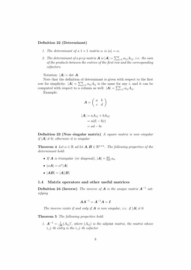
Definition 22 (Determinant)

1. The determinant of a 1× 1 matrix α is |α| = α.

2. The determinant of a p×p matrix A is |A| =∑p

j=1 a1jA1j, i.e. the sumof the products between the entries of the first row and the correspondingcofactors.

Notation: |A| = det A.Note that the definition of determinant is given with respect to the first

row for simplicity. |A| =∑p

j=1 aijAij is the same for any i, and it can becomputed with respect to a column as well: |A| =

∑pi=1 aijAij .

Example:

A =

(a bc d

)

|A| = aA11 + bA12

= a|d| − b|c|= ad− bc

Definition 23 (Non–singular matrix) A square matrix is non–singularif |A| 6= 0; otherwise it is singular

Theorem 4 Let α ∈ R ad let A,B ∈ Rn×n. The following properties of thedeterminant hold:

• If A is triangular (or diagonal), |A| =∏

i aii

• |αA| = αn|A|

• |AB| = |A||B|

1.4 Matrix operators and other useful matrices

Definition 24 (Inverse) The inverse of A is the unique matrix A−1 sat-isfying

AA−1 = A−1A = I

The inverse exists if and only if A is non singular, i.e. if |A| 6= 0

Theorem 5 The following properties hold:

1. A−1 = 1|A|(Aij)

′, where (Aij) is the adjoint matrix, the matrix whosei, j–th entry is the i, j–th cofactor

8

2. (cA−1) = c−1A−1

3. (AB)−1 = B−1A−1

4. (A′)−1 = (A−1)′

The first property follows from the definition of determinant, the othersfrom the definition of inverse applied to AB. The following is the Wood-bury’s theorem on the inverse of a special combination of matrices

Theorem 6 Let A be a (k× k) invertible matrix whereas U and V are two(n× k) matrices with k ≤ n and β an arbitrary scalar. Define

S = (Ik + V ′A−1U)

where Ik is the k-dim identity matrix, then

(A + βUV ′)−1 = A−1 − βA−1US−1V A−1 (1)

Proof : See Woodbury, A. (1950).

Theorem 7 Let A be a (n × n) nonsingular matrix and let A11 and A22

two submatrices of dimension (n1 × n1) and (n2 × n2) respectively, and let

A =

(A11 A12

A21 A22

)then

A−1 =

(A−1

11 + A−111 A12Ω22A21A

−111 −A−1

11 A12Ω22

−Ω22A21A−111 Ω22

)with Ω22 = (A22 −A21A

−111 A12)−1 and

A−1 =

(Ω11 −A−1

22 A21Ω11

−A−122 A21Ω11 A−1

22 + A−122 A21Ω11A12A

−122

)with Ω11 = (A11 −A12A

−122 A21)−1.

Proof By definition the inverse of A is a matrix Ω = A−1 such thatA−1A = AA−1 = I with In n-dimensional identity matrix, thus(

Ω11 Ω12

Ω21 Ω22

)(A11 A12

A21 A22

)=

(In1 00 In2

)and (

A11 A12

A21 A22

)(Ω11 Ω12

Ω21 Ω22

)=

(In1 00 In2

)

9

The two parts of the definition give the following systems of equationsΩ11A11 + Ω11A21 = In1

Ω11A12 + Ω12A22 = 0Ω21A11 + Ω22A21 = 0Ω21A12 + Ω22A22 = In2

and A11Ω11 + A12Ω21 = In1

A11Ω12 + A12Ω22 = 0A21Ω11 + A22Ω21 = 0A21Ω12 + A22Ω22 = In2

respectively.From the first system we have

Ω12 = (A21 −A22A−112 A11)−1

Ω11 = −Ω12A22A−112

Ω21 = −Ω22A21A−111

Ω22 = (A22 −A21A−111 A12)−1

which allow us to find Ω22 and Ω21 as a function of Ω22.From the second system we have

Ω11 = (A11 −A12A−122 A21)−1

Ω12 = −A−111 A

−112 Ω22

Ω21 = −A−122 A21Ω11

Ω22 = (A22 −A21A−111 A12)−1

which allow us to find Ω12 as a function of Ω22. In order to find Ω11 we usethe first equation from the second system and the value of Ω21 from the firstsystem

A11Ω11 + A12(−Ω22A21A−111 ) = In1

⇔ Ω11 = A−111 + A−1

11 A12Ω22A21A−111

The following properties hold for

1. the determinant of a partitioned matrix A =

(A11 A12

A21 A22

),

|A| = |A11||A22 −A21A−111 A12| = |A22||A11 −A12A

−122 A21|

2. the determinant of the sum of two matrices B(p × n) and C(n × p),|A + BC| = |A||Ip + A−1BC| = |A||In + CA−1B|

10

Definition 25 (Moore-Penrose Pseudoinverse) Let A a (n × m) realmatrix, then the A† matrix is called Moore-Penrose pseudoinverse if it sat-isfies:

1. AA†A = A

2. A†AA† = A†

3. (AA†)′ = AA†

4. (A†A)′ = A†A

Note that if A has linearly independent column then A† = (A′A)−1A′ iscalled left pseudoinverse matrix and A†A = I.

Definition 26 (Kronecker product) Let A be a (n× p) matrix and B a(m× q) one. The Kronecker product of A and B is the (nm× pq) matrix

A⊗B =

a11B a12B . . . a1pBa21B a22B . . . a2pB...

......

an1B an2B . . . anpB

Definition 27 (Hadamard Product) Let A and B be two (n×p) matri-ces. The Hadamard product of A and B is the (n× p) matrix

AB =

a11b11 a12b12 . . . a1pb1pa21b21 a22b22 . . . a2pb2p

......

...an1bn1 an2bn2 . . . anpbnp

Definition 28 (Khatri-Rao Product) Let A be a (n× p) matrix and Ba (m× p) one. The Khatri-Rao product of A and B is the (nm× p) matrix

A ∗B =(a1 ⊗ b1 a2 ⊗ b2 . . . ap ⊗ bp

)Definition 29 (Vectorization) Let A be a (n× p) matrix. The vec of Ais the nm-dimensional vector

vecA =

a1

a2...ap

11

Definition 30 (Matricization (or unfolding, or flattening)) The mode-n matricization of a tensor A ∈ RI1×···×IN is denoted by A(n) and arrangethe n-mode fibers to be the columns of the resulting matrix. The (im, j)-thelement of the matrix A(n) corresponds to the (i1, i2, · · · , iN )-th element ofA with

j = 1 +

N∑k=1,k 6=n

(ik − 1)Jk, with Jk =

k−1∏m=1,m 6=n

Im

Theorem 8 The Kronecker product satisfies the following properties:

1. (A⊗B)′ = (A′ ⊗B′)

2. (A⊗ (B ⊗C)) = ((A⊗B)⊗C) = (A⊗B ⊗C)

3. (A⊗ (B + C)) = ((A⊗B) + (A⊗C))

4. (A⊗B)(C ⊗D) = (AC ⊗BD)

5. |(A ⊗ B)| = |A|m|B|n where A and B are n- and m-dimensionalsquare conformable matrices, respectively.

6. (A⊗B)−1 = (A−1 ⊗B−1)

7. (A⊗B)† = (A† ⊗B†)

8. tr (A⊗B) = tr A tr B

Theorem 9 Let A a (n ×m) matrix, B a (m × p) and C a (p × q). TheKronecker products satisfies the following relationships with the vec operator

1. vec(AB) = (Ip ⊗A)vecB = (B′ ⊗ In)vecA

2. vec(ABC) = (C ′ ⊗A)vecB

3. vec(ABC) = (Iq ⊗AB)vecC = (C ′B′ ⊗ Im)vecA

Theorem 10 Let A a (n×m) matrix, B a (m× p) and C a (p× n). TheKronecker products satisfies the following relationships with the vec and troperators

1. tr (AB) = vec(B′)′vec(A) = vec(A′)′vec(B)

2. tr (ABC) = vec(A′)′(C ′ ⊗ Im)vec(B) = vec(A′)′(In ⊗B)vec(C) =vec(B′)′(A′ ⊗ Ip)vec(C) = vec(B′)′(Im ⊗C)vec(A)

Theorem 11 The Hadamard and Khatri-Rao products satisfies the follow-ing properties:

1. A ∗B ∗C = (A ∗B) ∗C = A ∗ (B ∗C)

12

2. (A ∗B)′(A ∗B) = A′AB′B

3. (A ∗B)† = (A′AB′B)†(A ∗B)′

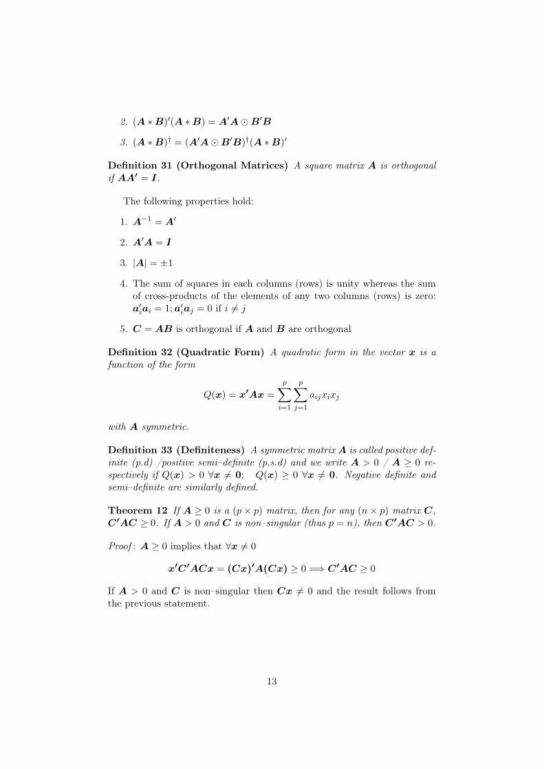
Definition 31 (Orthogonal Matrices) A square matrix A is orthogonalif AA′ = I.

The following properties hold:

1. A−1 = A′

2. A′A = I

3. |A| = ±1

4. The sum of squares in each columns (rows) is unity whereas the sumof cross-products of the elements of any two columns (rows) is zero:a′iai = 1;a′iaj = 0 if i 6= j

5. C = AB is orthogonal if A and B are orthogonal

Definition 32 (Quadratic Form) A quadratic form in the vector x is afunction of the form

Q(x) = x′Ax =

p∑i=1

p∑j=1

aijxixj

with A symmetric.

Definition 33 (Definiteness) A symmetric matrix A is called positive def-inite (p.d) /positive semi–definite (p.s.d) and we write A > 0 / A ≥ 0 re-spectively if Q(x) > 0 ∀x 6= 0; Q(x) ≥ 0 ∀x 6= 0. Negative definite andsemi–definite are similarly defined.

Theorem 12 If A ≥ 0 is a (p× p) matrix, then for any (n× p) matrix C,C′AC ≥ 0. If A > 0 and C is non–singular (thus p = n), then C′AC > 0.

Proof : A ≥ 0 implies that ∀x 6= 0

x′C′ACx = (Cx)′A(Cx) ≥ 0 =⇒ C′AC ≥ 0

If A > 0 and C is non–singular then Cx 6= 0 and the result follows fromthe previous statement.

13

2 Vector Spaces

2.1 Geometry of 2× 1 vectors

• 2× 1 geometrical vector

A 2×1 vector has a natural representation on a standard x–y coordinatesystem as a segment from the origin to a given point P :

P (u1, u2) −→ u = [u1 u2]′

The sum of two 2–dimensional geometrical vectors has a natural geo-metrical meaning:

u + v = [u1 u2]′ + [v1 v2]′ = [u1 + v1 u2 + v2]′

14

The parallelogram rule: place the tail of a vector parallel to v and withv’s length on the head of vector u. Call the "sum" of the two vectorsthe new vector u + v connecting the tail of u with the head of v.

The length of a geometric vector, the shortest distance between its tailand its head, can be derived by Pythagorean theorem:

d =√u2

1 + u22 = (u′u)1/2

Therefore, the matrix product u′v = u1v1 + u2v2 = 0 has a geometricmeaning: u′v = 0 implies that the two vectors are orthogonal. Sincethe slope of u is u2/u1, and the slope of v is v2/v1, it is easily to checkthat the two vectors are perpendicular. The product of their slopes(u2/u1)(v2/v1) equals −1. Rewriting it, u1v1 + u2v2 = 0.

2.2 Algebraic Structures

We start this part introducing a definition of binary operation. We seewhen it is internal or external with respect to a set. Then we describe thecharacteristics of an algebraic structure.

Definition 34 (Binary Operation) Let A,B,C be sets. We define a bi-nary operation any application ϕ : A × B → C. If A = B = C we can saythat ϕ : A×A→ A is an internal binary operation on A.

For algebric structure we mean a n-tuple formed by sets and operationon themselves. The simplest one is a couple (X,ϕ) where X is a set andϕ : X ×X → X is an internal binary operation on X

Definition 35 Given (X,ϕ)

15

1. The operation ϕ is called associative if ∀x, y, z ∈ X, (xϕy)ϕz = xϕ(yϕz).

2. The operation ϕ is called commutative if ∀x, y ∈ X, xϕy = yϕx.

3. An element u ∈ X is neutral with respect to the operation ϕ if ∀x ∈ X,xϕu = uϕx = x.

4. If (X,ϕ) admits the neutral element u, an element x ∈ X is calledinvertible if ∃x′ ∈ X, xϕx′ = x′ϕx = u. In this case, x and x′ arecalled opposites.

Now, we focus on a special algebraic structure (X,+, ∗) formed by a setX and by two internal operations on X.

• The latter operation + is called addition, it is associative and commu-tative, (X,+) admits neutral element, denoted by 0.

• The former operation ∗ is called multiplication, it is associative, (X, ∗)admits neutral element, denoted by 1.

If ∀x, y, z ∈ X, x∗(y+z) = (x∗y)+(x∗z) and (y+z)∗x = (y∗x)+(z∗x),we can say that the multiplication is distributive with respect to the addition.

Definition 36 (External Binary Operation) V is a set and K is an al-gebraic structure (K,+, ∗). (i.e., the set R of real numbers or the set Cof complex numbers). Any application ϕ such that K × V → V is said anexternal operation on V with coefficients in K.

2.3 Vector Spaces

Definition 37 (Vector Space) We define a vector space on K an algebraicstructure V = (K,V ,⊕,), formed by an algebraic structure K = (K,+, ∗)with 0 and 1 as respective neutrals, a set V , an internal operation ⊕ on V :

⊕ : V × V → V

and an external operation on V with coefficients in K:

: K× V → V

satisfying the following axioms:

SV1 The algebraic structure (V ,⊕) is commutative, associative, admits theneutral element and the opposite for each own element.

SV2 ∀α and ∀β ∈ K and v,w ∈ V

(i) (α+ β) v = (α v)⊕ (β v)

16

(ii) α (v ⊕w) = (α v)⊕ (αw)

(iii) α (β v) = (α ∗ β) v

(iv) 1 v = v

If K is R, then we have a real vector space. If K is C, then we have acomplex vector space.The elements of set V are called vectors and the elements of K are calledscalars.Operation ⊕ is said vector addition. Hereafter we denote it only with +.Operation is said multiplication by a scalar. Hereafter we denote it onlywith ∗. We often omit it. It is up to the reader to understand when theymean vector operation or when they mean internal operation in K.The unique neutral element of (V ,+) is called null vector and denoted by0. The unique opposite vector of a v ∈ V is denoted by −v.

Proposition 1 Let V be a vector space on K. For any α and β ∈ K andfor any v ∈ V, we have:

(i) αv = 0 if and only if α = 0 or v = 0;

(ii) (−α)v = α(−v) = −(αv);

(iii) if αv = βv and v 6= 0, then α = β

(iv) 1 v = v

• G3, the real vector space of all geometrical vectors in three-dimensionalphysical space.

• Rp (Cp), the real (complex) vector space of all real (complex) p × 1column matrices.

• Suppose that V and W are both real or both complex vector spaces.The product space V ×W is the vector space of ordered pairs (v,w)with v in V and with w in W , where

(v,w) + (v′,w′) = (v + v′,w + w′)

andα(v,w) = (αv, αw)

using the same scalars as for V .

Definition 38 (Subspaces) Suppose that V0 and V are both real or bothcomplex vector spaces, that V 0 is a subset of V , and that the operations onelements of V 0 as V0-vectors are the same as the operations on them asV-vectors. Then V0 is said to be a subspace of V.

17

Theorem 13 (Subspace Theorem) Suppose that V is a vector space andthat V 0 is a subset of V ; define vector addition and multiplication by scalarsfor elements of V 0 exactly as in V . Then V0 is a subspace of V if and onlyif the following three conditions hold:

1. V0 is nonempty.

2. V0 is closed under multiplication in the sense that αv0 is in V0, ∀v0

in V0 and all scalars α.

3. V0 is closed under vector addition in the sense that v0 + v′0 is in V0

for all vectors v0 in V0 and v′0 in V0.

Example 1 Suppose that v1,v2, . . . ,vr is some nonempty set of vectorsfrom V . Define V 0 as the set of all linear combinations

v0 = α1v1 + α2v2 + · · ·+ αrvr

where the scalars αi are allowed to range over all arbitrary values.Then V0 is a subspace of V. (Prove it using the Subspace Theorem)

2.4 Linear dependence and linear independence

Definition 39 (Linear Combination) A linear combination of the vec-tors v1,v2, . . . ,vn is an expression of the form α1v1 + α2v2 + . . . + αnvn

where the αi are scalars.

Definition 40 (Linear Dependence) A vector v is said to be linearly de-pendent on the set of vectors v1,v2, . . . ,vn if and only if can be written assome linear combination of v1,v2, . . . ,vn; otherwise v is said to be linearlyindependent of the set of vectors.

Definition 41 (Spanning Set) A set S of vectors v1,v2, . . . ,vn in V issaid to span (or generate) some subspace V0 of V if and only if S is a subsetof V 0 and every vector v0 in V 0 is linearly dependent on S; S is said to bea spanning set or generating set for V0.

A natural spanning set for R3 is the set of three unit vectors.

e1 =

100

e2 =

010

e3 =

001

A four vectors set, where at least three are linearly independent, is stilla spanning set of R3.

Therefore, given a spanning set S we can always delete all the linearlydependent vectors and still obtain a spanning set of linearly independentvectors.

18

Definition 42 Let L = v1,v2, . . . ,vn be a nonempty set of vectors.

• Suppose thatα1v1 + α2v2 + . . .+ αkvk = 0

implies that α1 = α2 = . . . = αk = 0. Then, L is said to be linearlyindependent.

• A set that is not linearly independent is said to be linearly dependent.Equivalently, L is linearly dependent if and only if there are scalarsα1, α2, . . . , αk not all zero, with

α1v1 + α1v2 + . . .+ αkvk = 0

Example 2 The set 1, 2− 3t, 4 + t is linearly dependent in the vectorspace P3 of polynomials of degree strictly less than three. To determine this,suppose that

α1(1) + α2(2− 3t) + αk(4− t) = 0

that means, for all t

(α1 + 2α2 + 4α3) + (−3α2 + α3)t = 0.

Then, we get α1 + 2α2 + 4α3 = 0

−3α2 + α3 = 0

a system of two equations for the three αi. The general solution is α1 =−10k

3 , α2 = k3 where k = α3.

Theorem 14 (Linear Independence)

• Suppose that L = v1,v2, . . . ,vn with k ≥ 2 and with all the vectorsvi 6= 0. Then L is linearly dependent if and only if at least one of thevj is linearly dependent on the remaining vectors vi where i 6= j.

• Any set containing 0 is linearly dependent.

• v is linearly independent if and only if v 6= 0.

• Suppose that v is linearly dependent on a set L = v1,v2, . . . ,vkand that vj is linearly dependent on the others in L, namely L′j =v1,v2, . . . ,vj−1,vj+1, . . . ,vk. Then v is linearly dependent on L′j

19

2.5 Basis and dimension

Definition 43 (Basis) A basis for a vector space V is a linearly indepen-dent spanning set for V .

Example 3 Recalling the definition of a spanning set, the vectors formingthe basis should belong to the vector space. We seek a basis for the subspaceV0 of R3 consisting of all solutions to x1 + x2 + x3 = 0. We can try withe1, e2, e3. These vector are linearly independent and any vector in R3 is alinear combination of these three. Any vector in V0 is a linear combinationof these three, as well. So we can say that e1, e2, e3 is a basis for R3 butnot for V0 because they do not belong to V0.A solution for x1 + x2 + x3 = 0 could be x1 = α and x2 = β, so thatx3 = −α− β. The general vector

v0 =

x1

x2

x3

=

αβ

−α− β

= αv1 + βv2

where

v1 =

10−1

,v2 =

01−1

form a basis for V0.

Theorem 15 (Unique basis representation theorem) Let B = v1 . . .vrbe a basis. Then the representation of each v with respect to B is unique: ifv = α1v1 + · · ·+ αrvr and v = α′1v1 + · · ·+ α′rvr, then ∀i, αi = α′i.

Definition 44 (Dimension) The number of vectors in a basis for a vectorspace is called dimension of the vector space.

Example 4 In R3 each element v can be decomposed as

v = v1e1 + v1e3 + v3e3

Now, we would like to represent the element v of R3 in a new coordinatesystem with basis e1, e2, e3. Thus we find the coefficients vj satisfyingvj = v · ej that is

v = (e1, e2, e3)′(e1, e2, e3)v

The matrix Q = (e1, e2, e3)′(e1, e2, e3) defines the change of coordinate. Thetransformation Q is geometrically a rotation map and satisfies the property

1. Q′Q = I

2. Q′ = Q−1

20

that is called orthonormality.

Example 5 The space of N -order tensors in ×RI×...×I with I = 3, endowedwith tensor summation and scalar multiplication

1. A + B is a N -order tensor with elements (ai1···iN + bi1···iN )

2. αA is a N -order tenor with elements αai1···iN

with A,B ∈ RI×I and α ∈ R, is a vector space. The set of N -order tensorsei1 ∨ · · · ∨ eiN , eil ∈ R3, l = 1, . . . , N is a basis for vector space.

Thus, the tensor A can be decomposed as

A =3∑

i1=1

· · ·3∑

iN=1

ai1···iN (ei1 ∨ · · · ∨ eiN )

Example 6 Let A ∈ R3×...×3 a N -order tensor and let ei1 ∨ . . .∨eiN , eil ∈R3, ∀l be the canonical orthonormal basis. The change of coordinates canbe defined as

aj1···jN = AN (ej1 ∨ · · · ∨ ejN )

=

∑i1,··· ,iN

ai1···iN (ei1 ∨ · · · ∨ eiN )

N (ej1 ∨ · · · ∨ ejN )

=

∑i1,··· ,iN

ai1···iN (ei1 · ej1) (ei2 ∨ · · · ∨ eiN )

N−1 (ej2 ∨ · · · ∨ ejN )

=∑

i1,··· ,iN

ai1···iN (ei1 · ej1) · · · (eiN · ejN )

where ei1 ∨ · · · ∨ eiN , eil ∈ R3, ∀l is a basis in the new coordinate system.When N = 2 we can write A = QAQ′

2.6 Matrix rank

Definition 45 Let A be a p× q matrix

1. The real (or complex) column space of A is the subspace of Rp (or Cp)that it is spanned by the set of columns of A.

2. The real (or complex) row space of A is the subspace of real (or com-plex) vector space of all real (or complex) 1 × q matrices that it isspanned by the set of the rows of A.

The rank of a matrix A is equal to the dimension of the row space or ofthe column space.

21

• The row space dimension is equal to the column space dimension.

Think to a p×p full rank matrix. This is invertible, so it is its transpose.Therefore A′ rank is the same as A rank

• In a p× q matrix the rank is at most minp, qThink to a 3× 4 matrix: If three columns are linearly independent, wehave three 3 × 1 vectors spanning R3, therefore the fourth is linearlydependent

2.7 Norms

Definition 46 A norm (or vector norm) on V is a function that assigns toeach vector v in V a non-negative real number, called the norm of v anddenoted by ‖ v ‖ satisfying:

1. ‖ v ‖> 0 for v 6= 0, and ‖ 0 ‖= 0.

2. ‖ αv ‖=| α |‖ v ‖ for all scalars α and vectors v.

3. ‖ u+v ‖≤‖ u ‖ + ‖ v ‖ for all vectors u and v (the triangle inequality).

Definition 47 (Norms) For vectors x = [x1x2 . . . xp]′ in Rp or Cp, the

norms ‖ · ‖1,‖ · ‖2, and ‖ · ‖∞ (called the 1-norm, 2-norm, ∞-norm) aredefined as

‖ x ‖1=| x1 | + | x2 | + . . .+ | xp |‖ x ‖2= (| x1 |2 + | x2 |2 + . . .+ | xp |2)1/2

‖ x ‖∞= max | x1 |, | x2 |, . . . , | xp | .(2)

Theorem 16 (Schwarz inequality) Let x and y be p×1 column matrices.Then

| xHy |≤‖ x ‖2‖ y ‖2where xH is the hermitian transpose, namely a matrix formed by the complexconjugates of the entries of the transpose matrix.

2.8 Inner product

We want to size the angle between the geometrical vectors a = [a1 a2]′ andb = [b1 b2]′ (see Figure 2.8).

From trigonometry we have that

|AB|2 = |OA|2 + |OB|2 − 2|OA||OB|cosθ

22

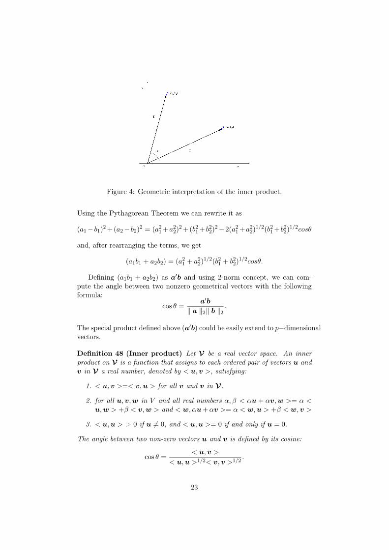
Figure 4: Geometric interpretation of the inner product.

Using the Pythagorean Theorem we can rewrite it as

(a1− b1)2 +(a2− b2)2 = (a21 +a2

2)2 +(b21 + b22)2−2(a21 +a2

2)1/2(b21 + b22)1/2cosθ

and, after rearranging the terms, we get

(a1b1 + a2b2) = (a21 + a2

2)1/2(b21 + b22)1/2cosθ.

Defining (a1b1 + a2b2) as a′b and using 2-norm concept, we can com-pute the angle between two nonzero geometrical vectors with the followingformula:

cos θ =a′b

‖ a ‖2‖ b ‖2.

The special product defined above (a′b) could be easily extend to p−dimensionalvectors.

Definition 48 (Inner product) Let V be a real vector space. An innerproduct on V is a function that assigns to each ordered pair of vectors u andv in V a real number, denoted by < u,v >, satisfying:

1. < u,v >=< v,u > for all v and v in V.

2. for all u,v,w in V and all real numbers α, β < αu + αv,w >= α <u,w > +β < v,w > and < w, αu+αv >= α < w,u > +β < w,v >

3. < u,u > > 0 if u 6= 0, and < u,u >= 0 if and only if u = 0.

The angle between two non-zero vectors u and v is defined by its cosine:

cos θ =< u,v >

< u,u >1/2< v,v >1/2.

23

Theorem 17 (Schwarz inequality) Let < u,v > be an inner product onthe real vector space V. Then |< u,v >|≤< u,u >1/2< v,v >1/2 for allu,v ∈ V.

Theorem 18 (Inner product norms) Let < u,v > be an inner producton the real vector space V, and define ‖ v ‖=< v,v >1/2. Then ‖ · ‖ is anorm on V induced by the inner product.

Definition 49 (Orthogonality) Let < ·, · > be an inner product on V andlet ‖ · ‖ be its induced norm.

1. Two vectors u and v are said to be orthogonal if and only if < u,v >=0 in that set.

2. A set of vectors is said to be orthogonal if and only if every two vectorsfrom the set are orthogonal: < u,v >= 0 ∀u 6= v.

3. If a non-zero vetor u is used to produce v = u‖u‖ so that ‖ v ‖= 1, then

u is said to have been normalized to produce the normalized vector v.

4. A set of vectors is said to be orthonormal if and only if the set isorthogonal and ‖ v ‖= 1 for all v in the set.

In any vector space with an inner product, 0 is orthogonal to every vector.

2.9 Other products

Definition 50 (Cross Product) Let V be a real vector space. A crossproduct on V is a function that assigns to each ordered pair of vectors u andv in V a real number, denoted by w = u× v, satisfying:

1. < w,u >=< w,v >= 0 for all v and u in V.

2. the direction of w is such that the triple (w,u,v) is right-handed.

The magnitude of w is:

< w,w >= sin θ < u,u >1/2< v,v >1/2

with 0 ≤ θ ≤ π.

Geometrically, the norm of the vector u× v represents the area of the par-allelogram having sides u and v.

Theorem 19 The cross product satisfies the following properties

1. u× v = −v × u (anti-symmetry)

2. w × (αv + βu) = αw × v + βw × u (linearity)

24

with α, β ∈ R.

Note that in any orthonormal system it holds that

e1 × e1 = 0, e1 × e2 = e3, e1 × e3 = −e2

e2 × e1 = −e3, e2 × e2 = 0, e2 × e3 = −e1

e3 × e1 = e2, e3 × e2 = −e1, e3 × e3 = 0

Thus we for any two vectors u and v we have

u× v =

∣∣∣∣∣∣e1 e2 e3

u1 u2 u3

v1 v2 v3

∣∣∣∣∣∣which in index notation is u × v = εijkujvkei where εijk is the Levi-Civitasymbol denoting the (i, j, k)-th element of a third-order tensor defined as

εijk =

+1 (i, j, k) is an even permutation of (1, 2, 3)−1 (i, j, k) is an odd permutation of (1, 2, 3)

0 otherwise, i.e. i = j, or j = k, or k = i

Definition 51 (Cross Tensor Vector Product) Let A be a third-ordertensor and u a vector then the cross product between vector and tensor isdefined as

A× u = εjmnaimunei ∨ ej

u×A = εimnumanjei ∨ ej

Definition 52 (Triple Product) Let V be a real vector space. A tripleproduct on V is a function that assigns to each ordered triplet of vectors u,v and w in V a real number w · (u× v) = εijkwiujvk.

Geometrically, the triple product of three vectors equals the volume of theparallelepiped with sides u, v and w.

Theorem 20 For the dot and cross-product the following properties hold:

1. u× (v ×w) = (u ·w)v − (u · v)w

2. (u× v)×w = (u ·w)v − (v ·w)u

3. (u× v) · (w × z) = (u ·w)(v · z)− (v · z)(v ·w)

4. (u× v)× (w × z) = (u · (v × z))w − (u · (v ×w))z

25

3 Differential calculus

3.1 Matrix differential calculus

Let g(A,x) be a real valued function with A a (n×m)-dimensional matrixand x a (n × 1)-dimensional vector. Let g(x) be a p vector of real valuedfunctions with i-th element gi(x), i = 1, . . . , p, a real valued function of then-vector x, then

1. ∂g/∂x is a (n × 1) vector with the i-the element given by ∂g/∂xi,i = 1, . . . , n

2. ∂g/∂A is a (n × m) matrix with (i, j)-th element given by ∂g/∂aij ,i = 1, . . . , n, j = 1, . . . ,m

3. ∂g/∂x′ is a (p× n) matrix with (i, j)-th element given by ∂gi/∂xj

Theorem 21 Let x and x two n-dimensional vectors, A and F two n-dimensional square matrices, y a p-dimensional vector and B a (p × n)-dimensional matrix. The following differential calculus rules apply

1. ∂a′x∂x = a

2. ∂a′x∂x′ = a′

3. ∂x′Ax∂x = (A + A′)x

4. ∂2x′Ax∂x∂x′ = (A + A′)

5. ∂y′Bx∂B = yx′

6. ∂tr (A)∂A = In

7. ∂tr (AF )∂A = F ′

8. ∂tr (AB′B)∂B = 2BA′

9. ∂|A|∂A = |A|(A′)−1(1− δ0(|A|))

10. ∂ log |A|∂A = (A′)−1 if |A| > 0

11. ∂ log |A′B′BA|∂A = 2B′BA(A′B′BA)−1 if |A′B′BA| > 0

Theorem 22 Let A be a (n ×m)-dimensional matrix with the (i, j)-th el-ement, aij(z), a function of the real variable z. Then let us define ∂A

∂z asthe (n × m) matrix with the (i, j)-th element ∂aij(z)

∂z . Then the followingproperties hold

26

12. ∂AB∂z = ∂A

∂z B + A∂B∂z

13. ∂A−1

∂aij= −A−1U ijA

−1 with U ij a matrix with (l, k)-th element givenby δi(l)δj(k) i, j = 1, . . . , n

14. ∂tr (A−1F )∂A = −A−1FA−1

15. ∂vec(A−1)∂vec(A)′ = −(A−1 ⊗A−1)

3.2 Tensor functions and fields

Let us focus on the tensors of the order two. A tensor function A(t) assignsa tensor A to a real number t, that is

Definition 53 (Tensor Function) A tensor function A is defined as

A =

[R→ SIt 7→ A(t)

where S = R3×3 is the space of the cubical tensors of order 2.

Definition 54 (Tensor Field) A tensor field A is defined as

A =

[R3 → S

x 7→ A(x)

where S = R3×3 is the space of the cubical tensors of order 2.

By applying the decomposition in Cartesian coordinates it is possible todefine the derivative of a differentiable tensor function

dA

dt= lim

t→0

A(t+ dt)−A(t)

dt=

3∑i=1

3∑j=1

limt→0

aij(t+ dt)− aij(t)dt

(ei ∨ ej)

which yields

dA

dt=

da11dt

da12dt

da13dt

da21dt

da22dt

da23dt

da31dt

da32dt

da33dt

Theorem 23 For tensor functions A(t), B(t) and C(t) and vector functiona(t), the following properties hold

1. ddt(A ·B) = dA

dt ·B + A · dBdt

2. ddt(A×B) = dA

dt ×B + A× dBdt

3. ddt(C · (A×B)) = dC

dt · (A×B) + C ·(dAdt ×B + A× dB

dt

)27

4. a · dadt = adadt

5. a · dadt = 0 iif ||a|| = c (constant), c ∈ R.

The differential dA of a tensor field A(x) depends on the direction of thedifferential of independent variable dx =

∑3i=1 xiei. When dx is parallel to

one of the coordinate axes we have

∂A

∂x1= lim

∆x1→0

A(x1 + ∆x1, x2, x3)−A(x1, x2, x3)

∆x1

the same applies to the partial derivatives with respect to x2 and x3. Thus

dA = grad(A) · dx =3∑

i=1

∂A

∂xi∨ ei · dx

=3∑

i=1

∂A

∂xi(ei · dx) =

3∑i=1

∂A

∂xi

ei ·3∑

j=1

dxjej

=

3∑i=1

3∑j=1

∂A

∂xidxjδij =

3∑i=1

∂A

∂xidxi

where δij = ei · ej is the Kronecker delta which takes value 0 if i 6= j and 1if i = j and where

grad(A) =3∑

i=1

∂A

∂xi∨ ei

denotes the gradient of A, which is a tensor of one order more higher thenA. By introducing the nabla operator

∇ =3∑

i=1

ei∂

∂xi

it followsgradA = A ∨∇

Definition 55 (Integral for Tensor Functions) Let A(t) and B(t) betensor functions such that B(t) = dA(t)/dt, then the indefinite integral ofA is ∫

A(t)dt = B(t) + C

By using the decomposition of the tensor function using the canonical basisin the Cartesian coordinate system it can be shown that the integration ofa tensor function comes down to integration of its components.

28

Definition 56 (Line Integral of a Tensor Field) Let A(x) be a tensorfield and C a space curve joining two points P1(x1, x2, x3) and P2(x1, x2, x3),and xi i = 1, . . . , N a set of poitns defining a partition of the curve, then theline integral of A is ∫

CA · dx = lim

N→∞

N∑i=1

A(xi) ·∆xi

where ∆xi = xi − xi−1 and maxi||∆xi|| → 0 as N →∞.

If the curve C can be parametrized in t with t ∈ [t1, t2] and x(t1) = P1 andx(t2) = P2 then the path integral becomes∫

CA · dx =

∫ t2

t1

A · dxdtdt

References

Kolda, T. G. and W. G. Bader (2009). Tensor decomposition and applica-tions. SIAM Rev 51(3), 455–500.

Magnus, J. R. and H. Neudecker (1999). Matrix Differential Calculus withApplications in Statistics and Econometrics, 2nd Edition. John Wiley.

Mardia, K. V., J. T. Kent, and J. M. Bibby (1979). Multivariate analysis.Probability and Mathematical Statistics, London: Academic Press.

Noble, B. and J. W. Daniel (1988). Applied Linear Algebra (3rd ed.). PrenticeHall.

Woodbury, A. (1950). Inverting modified matrices. Statist. Res. Group,Mem. Rep. No. 42, Princeton University, Princeton, NJ.

29