Matrices that commute with their derivative.On a letter from Schur to Wielandt. †

Olga Holtz‡ Volker Mehrmann‡ Hans Schneider §

Revision 13.10.2012

Abstract

We examine when a matrix whose elements are differentiable functions in one vari-able commutes with its derivative. This problem was discussed in a letter from IssaiSchur to Helmut Wielandt written in 1934, which we found in Wielandt’s Nachlass.We present this letter and its translation into English. The topic was rediscoveredlater and partial results were proved. However, there are many subtle observationsin Schur’s letter which were not obtained in later years. Using an algebraic setting,we put these into perspective and extend them in several directions. We present indetail the relationship between several conditions mentioned in Schur’s letter and wefocus in particular on the characterization of matrices called Type 1 by Schur. Wealso present several examples that demonstrate Schur’s observations.2000 Mathematics Subject Classification. 15A03, 15A27, 15A24, 15A16, 15A54Key words. Differential field, triangularization, diagonalization, matrix functions,commuting matrix functions.

1 Introduction

What are the conditions that force a matrix of differentiable functions to commute with itselementwise derivative? This problem, discussed in a letter from I. Schur to H. Wielandt[32], has been discussed in a large number of papers [2, 3, 4, 7, 9, 11, 12, 17, 19, 21, 22,23, 24, 27, 29, 31, 33, 34]. However, these authors were unaware of Schur’s letter anddid not find some of its principal results. A summary and a historical discussion of theproblem and several extensions thereof are presented by Evard in [14, 15], where the studyof the topic is dated back to the 1940s and 1950s, but Schur’s letter shows that it alreadyappeared in Schur’s lectures in the 1930s, if not earlier.

The content of the paper is as follows. In Section 2 we present a facsimile of Schur’sletter to Wielandt and its English translation. In Section 3 we discuss Schur’s letter and we

‡Institut fur Mathematik, Technische Universitat Berlin, Straße des 17. Juni 136, D-10623 Berlin, FRG.{holtz,mehrmann}@math.tu-berlin.de.§Department of Mathematics, University of Wisconsin, Madison, WI 53706, USA. hans@math.wisc.edu†Supported by Deutsche Forschungsgemeinschaft, through DFG project ME 790/15-2.

1

arX

iv:1

207.

1258

v5 [

mat

h.R

A]

26

Nov

201

2

motivate our use of differential fields. In Section 4 we introduce our notation and reproveFrobenius result on Wronskians. In Section 5 we discuss the results that characterize thematrices of Type 1 in Schur’s letter and in our main Section 6 we discuss the role played bydiagonalizability and triangularizability of the matrix in the commutativity of the matrixand its derivative. We also present several illustrative examples in Section 7 and we statean open problem in Section 8.

2 A letter from Schur to Wielandt

Our paper deals with the following letter from Issai Schur to his PhD student HelmutWielandt. See the facsimile below. Translated into English, the letter reads as follows:

Lieber Herr Doktor! Berlin, 21.7.34You are perfectly right. Already for 3 ≤ n < 6 not every solution of the equation

MM ′ = M ′M has the form

M1 =∑λ

fλCλ, (1)

where the Cλ are pairwise commuting constant matrices. One must also consider the type

M2 = (fαgβ), (α, β = 1, . . . n), (2)

where f1, . . . fn, g1, . . . , gn are arbitrary functions that satisfy the conditions∑α

fαgα =∑α

f ′αgα = 0

and therefore also ∑α

fαg′α = 0.

In this case we obtainM2 = MM ′ = M ′M = 0.

In addition we have the typeM3 = φE +M2, (3)

with M2 of type (2). ∗ From my old notes, which I did not present correctly in my lectures, itcan be deduced that for n < 6 every solution of MM ′ = M ′M can be completely decomposedby means of constant similarity transformations into matrices of type (1) and (3). Onlyfrom n = 6 on there are also other cases. This seems to be correct. But I have not checkedmy rather laborious computations (for n = 4 and n = 5).

I concluded in the following simple manner that one can restrict oneself to the casewhere M has only one characteristic root (namely 0): If M has two different characteristicroots, then one can determine a rational function N of M for which N2 = N but not

∗Note that E here denotes the identity matrix.

2

3

4

5

6

N = φE. Also N commutes with N ′. It follows from N2 = N that 2NN ′ = N ′, thus2N2N ′ = 2NN ′ = NN ′. This yields 2NN ′ = N ′ = 0, i.e., N is constant.

Now one can apply a constant similarity transformation to M so that instead of N oneachieves a matrix of the form [

E 00 0

].

This shows that M can be decomposed completely by means of a constant similarity trans-formation.

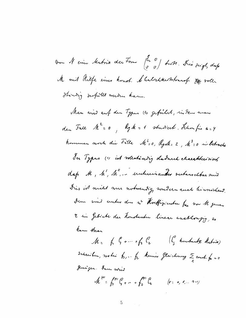
One is led to type (2) by studying the case M2 = 0, rankM = 1. Already for n = 4also the cases M2 = 0, rankM = 2, M3 = 0 need to be considered.

Type (1) is completely characterized by the property that M,M ′,M ′′, . . . are pairwisecommuting. This is not only necessary but also sufficient. For, if among the n2 coefficientsfαβ of M exactly r are linearly independent over the domain of constants, then one canwrite

M = f1C1 + · · ·+ frCr,

(Cs a constant matrix), where f1, . . . , fr satisfy no equation∑

α const fα = 0. Then

M (ν) = f(ν)1 C1 + · · ·+ f (ν)

r Cr, (ν = 1, . . . , r − 1).

Since the Wronskian determinant ∣∣∣∣∣∣∣ f1 . . . frf ′1 . . . f ′r

...

∣∣∣∣∣∣∣

cannot vanish identically, one obtains equations of the form

Cs =r−1∑σ=0

φsσM(σ).

If M,M ′,M ′′, . . . ,M (r−1) are pairwise commuting, then the same is true also for C1, . . . Crand thus M is of type (1). This implies furthermore that M belongs to type (1) if Mn is thehighest† power of M that equals 0. In the case n = 3 one therefore only needs to considertype (2).

With best regardsYours, Schur

†We think that Schur means lowest here.

7

3 Discussion of Schur’s letter

This letter was found in Helmut Wielandt’s mathematical Nachlass when it was collectedby Heinrich Wefelscheid and Hans Schneider not long after Wielandt’s death in 2001. Wemay therefore safely assume that Schur’s recent student Wielandt is the ”Herr Doktor” towhom the letter is addressed. Schur’s letter begins with a reference to a previous remarkof Wielandt’s which corrected an incorrect assertion by Schur. We can only guess at thissequence of events, but perhaps a clue is provided by Schur’s reference to his notes whichhe did not present correctly in his lectures. Could Wielandt have been in the audience anddid he subsequently point out the error? And what was this error? Very probably it wasthat every matrix of functions that commutes with its derivative is given by (1) (matricescalled Type 1), for Schur now denies this and displays another type of matrix commutingwith its derivative (called Type 2). He recalls that in his notes he claimed that for matricesof size 5 or less every such matrix is of Type 1, 2 or 3, where Type 3 is obtained from Type2 by adding a scalar function times the identity. This is not correct because there is alsothe direct sum of a size 2 matrix of Type 1 and a size 3 matrix of Type 2, we prove thisbelow.

We do not know why Schur was interested in the topic of matrices of functions thatcommute with their derivative, but it is probably a safe guess that this question came upin the context of solving differential equations, at least this is the motivation in many ofthe subsequent papers on this topic.

As one of the main results of his letter, Schur shows that an idempotent that commuteswith its derivative is a constant matrix and, without further explanation, concludes thatone can restrict oneself to matrices with a single eigenvalue. The latter observation raisesseveral questions. First, Schur does not say which functions he has in mind. Second,his argument follows from a standard decomposition of a matrix by a similarity into adirect sum of matrices provided that the eigenvalues of the matrix are functions of the typeconsidered. But this is not true in general, for example the eigenvalues of a matrix ofrational functions are algebraic functions. We wonder whether Schur was aware of thisdifficulty and we shall return to it at the end of this section.

Then Schur shows a matrix of size n is of Type 1 if and only if it and its first n − 1derivatives are pairwise commutative. His proof is based on a result of Frobenius [16] thata set of functions is linear independent over the constants if and only if their Wronskiandeterminant is nonzero. Frobenius, like Schur, does not explain what functions he hasin mind. In fact, Peano [28] shows that there exist real differentiable functions that arelinearly independent over the reals whose Wronskian is 0. This is followed by Bocher [5]who shows that Frobenius’ result holds for analytic functions and investigates necessaryand sufficient conditions in [6]. A good discussion of this topic can be found in [8].

We conclude this section by explaining how our exposition has been influenced by someof the observation above. As we do not know what functions Schur and Frobenius had inmind, we follow [1] and some unpublished notes of Guralnick [18] and set Schur’s resultsand ours in terms of differential fields (which include the field of rational functions and thequotient field of analytic functions over the real or complex numbers). Since we do not

8

know how Schur concludes that it is enough to consider matrices with a single eigenvalue,we derive our results from standard matrix decomposition (our Lemma 9 below) whichdoes not assume that all eigenvalues lie in the differential field under consideration.

4 Notation and preliminaries

A differential field F is an (algebraic) field together with an additional operation (thederivative), denoted by ′ that satisfies (a + b)′ = a′ + b′ and (ab)′ = ab′ + a′b for a, b ∈ F.An element a ∈ F is called a constant if a′ = 0. It is easily shown that the set of constantsforms a subfield K of F with 1 ∈ K. Examples are provided by the rational functions overthe real or complex numbers and the meromorphic functions over the complex numbers.

In what follows we consider a (differential) field F and matrices M = [mi,j] ∈ Fn,n. Themain condition that we want to analyze is when M ∈ Fn,n commutes with its derivative,

MM ′ = M ′M. (4)

As M ∈ Fn,n, it has a minimal and a characteristic polynomial, and M is called non-derogatory if the characteristic polynomial is equal to the minimal polynomial, otherwiseit is called derogatory. See [20].

In Schur’s letter the following three types of matrices are considered.

Definition 1 Let M ∈ Fn,n. Then M is said to be of

• Type 1 if

M =k∑j=1

fjCj,

where fj ∈ F, and Cj ∈ Kn,n, for j = 1, . . . , k, and the Cj are pairwise commuting;

• Type 2 ifM = fgT ,

with f, g ∈ Fn, satisfying fTg = fTg′ = 0;

• Type 3 ifM = hI + M,

with h ∈ F and M is of Type 2.

Schur’s letter also mentions the condition that all derivatives of M commute, i.e.,

M (i)M (j) = M (j)M (i) for all nonnegative integers i, j. (5)

To characterize the relationship between all these properties, we first recall several resultsfrom Schur’s letter and from classical algebra.

9

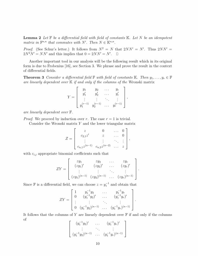
Lemma 2 Let F be a differential field with field of constants K. Let N be an idempotentmatrix in Fn,n that commutes with N ′. Then N ∈ Kn,n.

Proof. (See Schur’s letter.) It follows from N2 = N that 2NN ′ = N ′. Thus 2NN ′ =2N2N ′ = NN ′ and this implies that 0 = 2NN ′ = N ′.

Another important tool in our analysis will be the following result which in its originalform is due to Frobenius [16], see Section 3. We phrase and prove the result in the contextof differential fields.

Theorem 3 Consider a differential field F with field of constants K. Then y1, . . . , yr ∈ Fare linearly dependent over K if and only if the columns of the Wronski matrix

Y =

y1 y2 . . . yry′1 y′2 . . . y′r...

.... . .

...

y(r−1)1 y

(r−1)2 . . . y

(r−1)r

,are linearly dependent over F.

Proof. We proceed by induction over r. The case r = 1 is trivial.Consider the Wronski matrix Y and the lower triangular matrix

Z =

z 0 . . . 0

c2,1z′ z . . . 0

......

. . ....

cn,1z(n−1) cn,2z

(n−2) . . . z

,with ci,j appropriate binomial coefficients such that

ZY =

zy1 zy2 . . . zyr

(zy1)′ (zy2)

′ . . . (zyr)′

......

. . ....

(zy1)(n−1) (zy2)

(n−1) . . . (zyr)(n−1)

.Since F is a differential field, we can choose z = y−11 and obtain that

ZY =

1 y−11 y2 . . . y−11 yr0 (y−11 y2)

′ . . . (y−11 yr)′

......

. . ....

0 (y−11 y2)(n−1) . . . (y−11 yr)

(n−1)

.It follows that the columns of Y are linearly dependent over F if and only if the columnsof (y−11 y2)

′ . . . (y−11 yr)′

.... . .

...(y−11 y2)

(n−1) . . . (y−11 yr)(n−1)

10

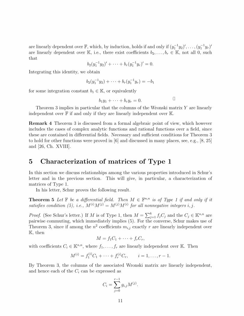
are linearly dependent over F, which, by induction, holds if and only if (y−11 y2)′, . . . , (y−11 yr)

′

are linearly dependent over K, i.e., there exist coefficients b2, . . . , br ∈ K, not all 0, suchthat

b2(y−11 y2)

′ + · · ·+ br(y−11 yr)

′ = 0.

Integrating this identity, we obtain

b2(y−11 y2) + · · ·+ br(y

−11 yr) = −b1

for some integration constant b1 ∈ K, or equivalently

b1y1 + · · ·+ bryr = 0.

Theorem 3 implies in particular that the columns of the Wronski matrix Y are linearlyindependent over F if and only if they are linearly independent over K.

Remark 4 Theorem 3 is discussed from a formal algebraic point of view, which howeverincludes the cases of complex analytic functions and rational functions over a field, sincethese are contained in differential fields. Necessary and sufficient conditions for Theorem 3to hold for other functions were proved in [6] and discussed in many places, see, e.g., [8, 25]and [26, Ch. XVIII].

5 Characterization of matrices of Type 1

In this section we discuss relationships among the various properties introduced in Schur’sletter and in the previous section. This will give, in particular, a characterization ofmatrices of Type 1.

In his letter, Schur proves the following result.

Theorem 5 Let F be a differential field. Then M ∈ Fn,n is of Type 1 if and only if itsatisfies condition (5), i.e., M (i)M (j) = M (j)M (i) for all nonnegative integers i, j.

Proof. (See Schur’s letter.) If M is of Type 1, then M =∑k

j=1 fjCj and the Cj ∈ Kn,n arepairwise commuting, which immediately implies (5). For the converse, Schur makes use ofTheorem 3, since if among the n2 coefficients mi,j exactly r are linearly independent overK, then

M = f1C1 + · · ·+ frCr,

with coefficients Ci ∈ Kn,n, where f1, . . . , fr are linearly independent over K. Then

M (i) = f(i)1 C1 + · · ·+ f (i)

r Cr, i = 1, . . . , r − 1.

By Theorem 3, the columns of the associated Wronski matrix are linearly independent,and hence each of the Ci can be expressed as

Ci =r−1∑j=0

gi,jM(j).

11

Thus, if condition (5) holds, then the Ci, i = 1, . . . , r, are pairwise commuting and thusM is of Type 1.

Using this result we immediately have the following Theorem.

Theorem 6 Let F be a differential field with field of constants K. If M ∈ Fn,n is non-derogatory and MM ′ = M ′M , then M is of Type 1.

Proof. If M is nonderogatory then all matrices that commute with M have the form p(M),where p is a polynomial with coefficients in F, see [10, 20]. Thus MM ′ = M ′M impliesthat M ′ is a polynomial in M . But then every derivative M (j) is a polynomial in M aswell and thus (5) holds which by Theorem 5 implies that M is of Type 1.

The following example from [4, 14] of a Type 2 matrix shows that one cannot easilydrop the condition that the matrix is nonderogatory.

Example 7 Let

f =

1tt2

, g =

t2

−2t1

,then fTg = 0 and fTg′ = 0, hence

Ma := gfT =

t2 t3 t4

−2t −2t2 −2t3

1 t t2

, (6)

is of Type 2. Since Ma is nilpotent with M2a = 0 but Ma 6= 0 and the rank is 1, it is

derogatory. One has

M ′a =

2t 3t2 4t3

−2 −4t −6t2

0 1 2t

, M ′′a =

2 6t 12t2

0 −4 −12t0 0 2

,and thus MaM

′a = M ′

aMa = 0. By the product rule it immediately follows that MaM′′a =

M ′′aMa, but

M ′aM

′′a =

4t 0 −4t3

−4 4t 12t2

0 −4 −8t

6= M ′aM

′′a =

−8t −6t2 −4t3

8 4t 00 2 4t

.Therefore, it follows from Theorem 5 that Ma is not of Type 1.

For any dimension n ≥ 3, one can construct an example of Type 2 by choosing f ∈ Fn,setting F = [f, f ′] and then choosing g in the nullspace of F T . Then fgT is of Type 2.

Actually every nilpotent matrix function M of rank one satisfying MM ′ = M ′M is of theform M = fgT and hence of Type 2. This follows immediately because if M = fgT andM2 = 0 then gTf = 0 and hence gTf ′ + (gT )′f = 0. Then it follows from MM ′ = M ′Mthat fgT (f(gT )′ + f ′gT ) = (gTf ′)fgT = (f(gT )′ + f ′gT )fgT = (gT )′ffgT which impliesthat gTf ′ = fTg′ and hence gTf ′ = fTg′ = 0.

12

6 Triangularizability and Diagonalizability

In his letter Schur claims that it is sufficient to consider the case that M ∈ Fn,n is triangularwith only one eigenvalue. This follows from his argument in case the matrix has its eigen-values in F, which could be guaranteed by assuming that this matrix is F-diagonalizableor even F-triangularizable. Clearly a sufficient condition for this to hold is that F is alge-braically closed, because then for every matrix in Fn,n the characteristic polynomial splitsinto linear factors.

Definition 8 Let F be a differential field and let H be a subfield of F. Then M ∈ Fn,n iscalled H-triangularizable (diagonalizable) if there exists a nonsingular T ∈ Hn,n such thatT−1MT is upper triangular (diagonal).

Using Lemma 2, we can obtain the following result for matrices M ∈ Fn,n that commutewith their derivative M ′, which is most likely well known but we could not find a reference.

Lemma 9 Let F be a differential field with field of constants K, and suppose that M ∈ Fn,nsatisfies MM ′ = M ′M . Then there exists an invertible matrix T ∈ Kn,n such that

T−1MT = diag(M1, . . . ,Mk), (7)

where the minimal polynomial of each Mi is a power of a polynomial that is irreducibleover F.

Proof. Let the minimal polynomial of M be µ(λ) = µ1(λ) · · ·µk(λ), where the µi(λ) arepowers of pairwise distinct polynomials that are irreducible over F. Set

pi(λ) = µ(λ)/µi(λ), i = 1, . . . , k.

Since the polynomials pi(λ) have no common factor, there exist polynomials qi(λ), i =1, . . . , k, such that the polynomials εi(λ) = pi(λ)qi(λ), i = 1, . . . , k, satisfy

ε1(λ) + · · ·+ εk(λ) = 1. (8)

Setting Ei = εi(M), i = 1, . . . , k and using the fact that µ(M) = 0 yields that

E1 + · · ·+ Ek = I, (9)

EiEj = 0, i, j = 1, . . . , k, i 6= j, (10)

E2i = Ei, i = 1, . . . , k. (11)

The last identity follows directly from (9) and (10). Since the Ei are polynomials in M andMM ′ = M ′M , it follows that the Ei commute with E ′i, i = 1, . . . k. Hence, by Lemma 2,Ei ∈ Kn,n, i = 1, . . . , k. By (9), (10), and (11), Kn is a direct sum of the ranges of the Eiand we obtain that, for some nonsingular T ∈ Kn,n,

Ei := T−1EiT = diag(0, Ii, 0), i = 1, . . . , k,

13

where the Ii are identity matrices of the size equal to the dimension to the range of Ei.This is a consequence of the fact that Ei is diagonalizable with eigenvalues 0 and 1. Sinceeach Ei commutes with M , we obtain that

Mi := T−1EiMT

= T−1EiMEiT

= diag(0, Ii, 0)T−1MT diag(0, Ii, 0)

= diag(0,Mi, 0), i = 1, . . . , k.

Now observe thatEiµi(Mi)Ei = T−1εi(M)µi(M)εi(M)T = 0,

since εi(λ)µi(λ) = µ(λ)qi(λ). Hence µi(Mi) = 0 as well. We assert that µi(λ) is the minimalpolynomial of Mi, for if r(Mi) = 0 for a proper factor r(λ) of mi(λ) then r(M)Πj 6=iµj(M) =0, contrary to the assumption that µ(λ) is the minimal polynomial of M .

Lemma 9 has the following corollary, which has been proved in a different way in [1]and [18].

Corollary 10 Let F be a differential field with field of constants K. If M ∈ Fn,n satisfiesMM ′ = M ′M and is F-diagonalizable, then M is K-diagonalizable.

Proof. In this case, the minimal polynomial of M is a product of distinct linear factorsand hence, the minimal polynomial of each Mi occurring in the proof of Lemma 9 is linear.Therefore, each Mi is a scalar matrix.

We also have the following Corollary.

Corollary 11 Let F be a differential field with field of constants K. If M ∈ Fn,n satisfiesMM ′ = M ′M and is F-diagonalizable, then M is of Type 1.

Proof. By Corollary 10, M = T−1 diag(m1, . . . ,mn)T with mi ∈ F and nonsingular T ∈Kn,n. Hence

M =n∑i=1

miT−1Ei,iT

where Ei,i is a matrix that has a 1 in position (i, i) and zeros everywhere else. Since allthe matrices Ei,i commute, M is of Type 1.

Remark 12 Any M ∈ Fn,n that is of rank one, satisfies MM ′ = M ′M and is not nilpotent,is of Type 1, since in this case M is F-diagonalizable. This follows by Corollary 11, sincethe minimal polynomial has the from (λ − c)λ for some c ∈ F. This means in particularfor a rank one matrix M ∈ Fn,n to be of Type 2 and not of Type 1 it has to be nilpotent.

For matrices that are just triangularizable the situation is more subtle. We have thefollowing theorem.

14

Theorem 13 Let F be a differential field with an algebraically closed field of constants K.If M ∈ Fn,n is Type 1, then M is K-triangularizable.

Proof. Any finite set of pairwise commutative matrices with elements in an algebraicallyclosed field may be simultaneously triangularized, see e.g., [30, Theorem 1.1.5]. Underthis assumption on K, if M is Type 1, then it follows that the matrices Ci ∈ Kn,n in therepresentation of M are simultaneously triangularizable by a matrix T ∈ Kn,n. Hence Talso triangularizes M .

Theorem 13 implies that Type 1 matrices have n eigenvalues in F if K is algebraicallyclosed and it further immediately leads to a Corollary of Theorem 6.

Corollary 14 Let F be a differential field with field of constants K. If M ∈ Fn,n isnonderogatory, satisfies MM ′ = M ′M and if K is algebraically closed, then M is K-triangularizable.

Proof. By Theorem 6 it follows that M is Type 1 and thus the assertion follows fromTheorem 13.

7 Matrices of small size and examples

Example 7 again shows that it is difficult to drop some of the assumptions, since thismatrix is derogatory, not of Type 1, and not K-triangularizable.

One might be tempted to conjecture that any M ∈ Fn,n that is K-triangularizable andsatisfies (4) is of Type 1 but this is so only for small dimensions and is no longer true forlarge enough n, as we will demonstrate below. Consider small dimensions first.

Proposition 15 Consider a differential field F of functions with field of constants K. LetM = [mi,j] ∈ F2,2 be upper triangular and satisfy MM ′ = M ′M . Then M is of Type 1.

Proof. Since MM ′ = M ′M we obtain

m1,2(m′1,1 −m′2,2)−m′1,2(m1,1 −m2,2) = 0,

which implies that m1,2 = 0 or m1,1 −m2,2 = 0 or both are nonzero and ddt

(m1,1−m2,2

m1,2) = 0,

i.e., cm1,2 + (m1,1 −m2,2) = 0 for some nonzero constant c.If m1,1 = m2,2 or m1,2 = 0, then M , being triangular, is obviously of Type 1. Otherwise

M = m1,1I +m1,2

[0 10 c

].

and hence again of Type 1 as claimed.

Proposition 15 implies that 2×2 K-triangularizable matrices satisfying (4) are of Type 1.

Proposition 16 Consider a differential field F with an algebraically closed field of con-stants K. Let M = [mi,j] ∈ F2,2 satisfy MM ′ = M ′M . Then M is of Type 1.

15

Proof. If M is F-diagonalizable, then the result follows by Corollary 11. If M is notF-diagonalizable, then it is nonderogatory and the result follows by Corollary 14.

Example 17 In the 2 × 2 case, any Type 2 or Type 3 matrix is also of Type 1 but notevery Type 1 matrix is Type 3.

Let M = φI2 + fgT with

φ ∈ F, f =

[f1f2

], g =

[g1g2

]∈ F2

be of Type 3, i.e., fTg = f ′Tg = fTg′ = 0.If f2 = 0, then M is upper triangular and hence by Proposition 15, M is of Type 1. If

f2 6= 0, then with

T =

[1 −f1/f20 1

].

we have

TMT−1 = φI2 +

[0 0f2g1 0

]= φI2 + f2g1

[0 01 0

],

since f1g1 + f2g2 = 0, and hence M is of Type 1.However, if we consider

M = φI2 + f

[0 c0 d

]with φ, f nonzero functions and c, d nonzero constants, then M is Type 1 but not Type 3.

Proposition 18 Consider a differential field F of functions with field of constants K. LetM = [mi,j] ∈ F3,3 be K-triangularizable and satisfy MM ′ = M ′M . Then M is of Type 1.

Proof. Since M is K-triangularizable, we may assume that it is upper triangular alreadyand consider different cases for the diagonal elements. If M has three distinct diagonalelements, then it is K-diagonalizable and the result follows by Corollary 11. If M hasexactly two distinct diagonal elements, then it can be transformed to a direct sum ofa 2 × 2 and 1 × 1 matrix and hence the result follows by Proposition 15. If all diagonalelements are equal, then, letting Ei,j be the matrix that is zero except for the position (i, j),

where it is 1, we have M = m1,1I + m1,3E1,3 + M , where M = m1,2E1,2 + m2,3E2,3 alsosatisfies (4). Then it follows that m1,2m

′2,3 = m′1,2m2,3. If either m1,2 = 0 or m2,3 = 0, then

we immediately have again Type 1, since M is a direct sum of a 2×2 and a 1×1 problem.If both are nonzero, then M is nonderogatory and the result follows by Theorem 6. Infact, in this case m1,2 = cm2,3 for some c ∈ K and therefore

M = m1,1I +m1,3E1,3 +m2,3

0 c 00 0 10 0 0

,16

which is clearly of Type 1.

In the 4 × 4 case, if the matrix is K-triangularizable, then we either have at leasttwo different eigenvalues, in which case we have reduced the problem again to the caseof dimensions smaller than 4, or there is only one eigenvalue, and thus without loss ofgenerality M is nilpotent. If M is nonderogatory then we again have Type 1. If M isderogatory then it is the direct sum of blocks of smaller dimension. If these dimensionsare smaller than 3, then we are again in the Type 1 case. So it remains to study the caseof a block of size 3 and a block of size 1. Since M is nilpotent, the block of size 3 is eitherType 1 or Type 2. In both cases the complete matrix is also Type 1 or Type 2, respectively.

The following example shows that K-triangularizability is not enough to imply that thematrix is Type 1.

Example 19 Consider the 9× 9 block matrix

M =

0 Ma 00 0 Ma

0 0 0

,where Ma is the Type 2 matrix from Example 7. Then M is nilpotent upper triangularand not of Type 1, 2, or 3, the latter two facts due to its F-rank being 2.

Already in the 5× 5 case, we can find examples that are none of the (proper) types.

Example 20 Consider M = T−1 diag(M1,M2)T with T ∈ Kn,n, M1 ∈ F3,3 of Type 2 (e.g.,

take M1 = Ma as in Example 7) and M2 =

[0 10 0

]. Then clearly M is not of Type 1 and

it is not of Type 2, since it has an F-rank larger than 1. By definition it is not of Type 3either. Clearly examples of any size can be constructed by building direct sums of smallerblocks.

Schur’s letter states that for n ≥ 6 there are other types. The following exampledemonstrates this.

Example 21 Let Ma be the Type 2 matrix in Example 7 and form the block matrix

A =

[Ma I0 Ma

].

Direct computation shows AA′ = A′A but A′A′′ 6= A′′A. Furthermore A3 = 0 and Ahas F-rank 3. Thus A is neither Type 1, Type 2 nor Type 3 (the last case need not beconsidered, since A is nilpotent). We also note that rank(A′′) = 6. We now assume thatK is algebraically closed and we show that A is not K-similar to the direct sum of Type 1or Type 2 matrices.

To obtain a contradiction we assume that (after a K-similarity) A = diag(A1, A2) whereA1 is the direct sum of Type 1 matrices (and hence Type 1) and A2 is the direct sum of

17

Type 2 matrices that are not Type 1. Since A is not Type 1, A2 cannot be the emptymatrix. Since the minimum size of a Type 2 matrix that is not Type 1 is 3 and its rankis 1 it follows that A cannot be the sum of Type 2 matrices that are not Type 1. Hencethe size of A1 must be larger or equal to 1 and, since A1 is nilpotent, it follows thatrank(A1) < size(A1). Since A1 is K-similar to a strictly triangular matrix, it follows thatrank(A′′1) < size(A1). Hence rank(A′′) = rank(A′′1) + rank(A′′2) < 6, a contradiction.

Example 22 If the matrix M =∑r

i=0Citi ∈ Fn,n is a polynomial with coefficients Ci ∈

Kn,n, then from (4) we obtain a specific set of conditions on sums of commutators thathave to be satisfied. For this we just compare coefficients of powers of t and obtain a set ofquadratic equations in the Ci, which has a clear pattern. For example, in the case r = 2,we obtain the three conditions C0C1−C1C0 = 0, C0C2−C2C0 = 0 and C1C2−C2C1 = 0,which shows that M is of Type 1. For r = 3 we obtain the first nontrivial condition3(C0C3 − C3C0) + (C1C2 − C2C1) = 0.

We have implemented a Matlab routine for Newton’s method to solve the set ofquadratic matrix equations in the case r = 3 and ran it for many different random startingcoefficients Ci of different dimensions n. Whenever Newton’s method converged (which itdid in most of the cases) it converged to a matrix of Type 1. Even in the neighborhoodof a Type 2 matrix it converged to a Type 1 matrix. This suggests that the matrices ofType 1 are generic in the set of matrices satisfying (4). A copy of the Matlab routine isavailable from the authors upon request.

8 Conclusion

We have presented a letter of Schur’s that contains a major contribution to the questionwhen a matrix with elements that are functions in one variable commutes with its deriva-tive. Schur’s letter precedes many partial results on this question, which is still partiallyopen. We have put Schur’s result in perspective with later results and extended it in analgebraic context to matrices over a differential field. In particular, we have presentedseveral results that characterize Schur’s matrices of Type 1. We have given examples ofmatrices that commute with their derivative which are of none of the Types 1, 2 or 3.Wehave shown that matrices of Type 1 may be triangularized over the constant field (whichimplies that their eigenvalues lie in the differential field) but we are left with an openproblem already mentioned in Section 3.

Open Problem 23 LetM be a matrix in a differential field F, with an algebraically closedfield of constants, that satisfies MM ′ = M ′M . Must the eigenvalues of M be elements ofthe field F?

For example, if M is a polynomial matrix over the complex numbers must the eigenvaluesbe rational functions? We have found no counterexample.

18

Acknowledgements

We thank Carl de Boor for helpful comments on a previous draft of the paper and OlivierLader for his careful reading of the paper and for his suggestions. We also thank ananonymous referee for pointing out the observation in Remark 12.

References

[1] W.A. Adkins, J.-C. Evard, and R.M. Guralnik, Matrices over differential fields whichcommute with their derivative, Linear Algebra Appl., 190:253–261, 1993.

[2] V. Amato, Commutabilita del prodotto di una matrice per la sua derivata, (Italian),Matematiche, Catania, 9:176–179, 1954.

[3] G. Ascoli, Sulle matrici permutabili con la propria derivata, (Italian), Rend. Sem.Mat. Univ. Politec. Torino, 9:245–250, 1950.

[4] G. Ascoli, Remarque sur une communication de M. H. Schwerdtfeger, (French), Rend.Sem. Mat. Univ. Politec. Torino, 11:335–336, 1952.

[5] M. Bocher, The theory of linear dependence, Ann. of Math. (2) 2:81–96, 1900/01.

[6] M. Bocher, Certain cases in which the vanishing of the Wronskian is a sufficientcondition for linear dependence, Trans. American Math. Soc. 2:139–149, 1901.

[7] Ju. S. Bogdanov and G. N. Cebotarev, On matrices which commute with their deriva-tives. (Russian) Izv. Vyss. Ucebn. Zaved. Matematika 11:27–37, 1959.

[8] A. Bostan and P. Dumas, Wronskians and linear independence, American Math.Monthly, 117:722–727, 2010.

[9] J. Dieudonne, Sur un theoreme de Schwerdtfeger, (French), Ann. Polon. Math.,XXIX:87–88, 1974.

[10] M.P. Drazin, J.W. Dungey, and K.W. Gruenberg, Some theorems on commutativematrices, J. London Math. Soc., 26:221–228, 1951.

[11] I.J. Epstein, Condition for a matrix to commute with its integral, Proc. AmericanMath. Soc., 14:266-270, 1963.

[12] N.P. Erugin, Privodimyye sistemy (Reducible systems), Trudy Fiz.-Mat. Inst. im. V.A.Steklova XIII, 1946.

[13] N.P. Erugin, Linear Systems of Ordinary Differential Equations with Periodic andQuasi-periodic Coefficients, Academic, New York, 1966.

19

[14] J.-C. Evard, On matrix functions which commute with their derivative, Linear AlgebraAppl., 68:145–178, 1985.

[15] J.-C. Evard, Invariance and commutativity properties of some classes of solutions ofthe matrix differential equation X(t)X ′(t) = X ′(t)X(t), Linear Algebra Appl., 218:89–102, 1995.

[16] F.G. Frobenius, Uber die Determinante mehrerer Functionen einer Variablen, (Ger-man), J. Reine Angew. Mathematik, 77:245–257, 1874. In Gesammelte AbhandlungenI, 141–157, Springer Verlag, 1968.

[17] S. Goff, Hermitian function matrices which commute with their derivative, LinearAlgebra Appl., 36:33–46, 1981.

[18] R. Guralnick, Private communication, 2005.

[19] M.J. Hellman, Lie algebras arising from systems of linear differential equations, Dis-sertation, Dept. of Mathematics, New York Univ., 1955.

[20] R.A. Horn and C.R. Johnson, Matrix Analysis, Cambridge University Press, Cam-bridge, UK 1985.

[21] L. Kotin and I.J. Epstein, On matrices which commute with their derivatives, Lin.Multilinear Algebra, 12:57–72, 1982.

[22] L.M. Kuznecova, Periodic solutions of a system in the case when the matrix of thesystem does not commute with its integral, (Russian), Differentsial’nye Uravneniya(Rjazan’), 7:151–161, 1976.

[23] J.F.M. Martin, On the exponential representation of solutions of systems of lineardifferential equations and an extension of Erugin’s theorem, Doctoral Thesis, StevensInst. of Technology, Hoboken, N.J., 1965.

[24] J.F.P. Martin, Some results on matrices which commute with their derivatives, SIAMJ. Ind. Appl. Math., 15:1171–1183, 1967.

[25] G.H. Meisters, Local linear dependence and the vanishing of the Wronskian, AmericanMath. Monthly, 68:847–856, 1961.

[26] T. Muir, A Treatise on the Theory of Determinants, Dover, 1933.

[27] I.V. Parnev, Some classes of matrices that commute with their derivatives (Russian),Trudy Ryazan. Radiotekhn. Inst., 42:142–154, 1972.

[28] G. Peano, Sur le determinant Wronskien, Mathesis 9, 75–76 & 110– 112, (1889).

[29] G. N. Petrovskii, Matrices that commute with their partial derivatives, Vestsi Akad.Navuk BSSR Minsk Ser. Fiz. i Mat. Navuk, 4:45-47, 1979.

20

[30] H. Radjavi and P. Rosenthal, Simultaneous Triangulation, Springer Verlag, Berlin,2000.

[31] N.J. Rose, On the eigenvalues of a matrix which commutes with its derivative, Proc.American Math. Soc., 4:752–754, 1965.

[32] I. Schur, Letter from Schur to Wielandt, 1934.

[33] H. Schwerdtfeger, Sur les matrices permutables avec leur derivee, (French), Rend.Sem. Mat. Univ. Politec. Torino, 11:329–333, 1952.

[34] A. Terracini. Matrici permutabili con la propia derivata, (Italian), Ann. Mat. PuraAppl. 40:99–112, 1955.

[35] E.I. Troickii, A study of the solutions of a system of three linear homogeneous differ-ential equations whose matrix commutes with its integral, (Russian), Trudy Ryazan.Radiotekhn. Inst., 53:109–115, 188-189, 1974.

[36] I.M. Vulpe, A theorem due to Erugin, Differential Equations, 8:1666–1671, 1972,transl. from Differentsial’nye Uravneniya, 8:2156–2162, 1972.

21