MATLAB® @ Work

richj@datatool.com www.datatool.com

Table Fundamentals Richard Johnson

A table is a MATLAB® container for storing column-oriented variables that have the same number of

rows. Unlike numerical or character arrays, the columns can have different data types. The table entries

can be addressed using row and column names or numbers. The concepts of object oriented

programming are helpful in understanding tables.

Tables were introduced in R2013b.

Contents

Data container .......................................................................................................................................... 2

Computing with tables .............................................................................................................................. 5

Sorting ....................................................................................................................................................... 7

Display and summary ................................................................................................................................ 9

Properties ................................................................................................................................................ 10

Methods .................................................................................................................................................. 12

Style ......................................................................................................................................................... 13

Other considerations .............................................................................................................................. 13

Review of table fundamentals ................................................................................................................ 13

Exercises .................................................................................................................................................. 14

Appendix ................................................................................................................................................. 15

2

Data container One of the main uses for a table in data analysis is as a container to hold data and metadata together.

You build a table from variables that all have the same number of rows. For example

importScores

TestScores = table(LastName, Gender, Test1, Test2, Test3)

TestScores =

LastName Gender Test1 Test2 Test3

__________ ________ _____ _____ _____

'HOWARD' 'male' 90 87 93

'WARD' 'male' 87 85 83

'TORRES' 'male' 86 85 88

'PETERSON' 'female' 75 80 72

'GRAY' 'female' 89 86 87

'RAMIREZ' 'female' 96 92 98

'JAMES' 'male' 78 75 77

'WATSON' 'female' 91 94 92

'BROOKS' 'female' 86 83 85

'KELLY' 'male' 79 76 82

The resulting table is 10x5 because there are 5 input variables, each with 10 rows.

You could instead specify table row names, which in this case produces a 10x4 table.

TestScores = table(Gender, Test1, Test2, Test3, 'RowNames', LastName)

TestScores =

Gender Test1 Test2 Test3

________ _____ _____ _____

HOWARD 'male' 90 87 93

WARD 'male' 87 85 83

TORRES 'male' 86 85 88

PETERSON 'female' 75 80 72

GRAY 'female' 89 86 87

RAMIREZ 'female' 96 92 98

JAMES 'male' 78 75 77

WATSON 'female' 91 94 92

BROOKS 'female' 86 83 85

KELLY 'male' 79 76 82

Note that the table constructor uses the variable names as column headers, which are stored in the

VariableNames field of the table properties.

disp(TestScores.Properties)

3

Description: ''

VariableDescriptions: {}

VariableUnits: {}

DimensionNames: {'Row' 'Variable'}

UserData: []

RowNames: {10x1 cell}

VariableNames: {'Gender' 'Test1' 'Test2' 'Test3'}

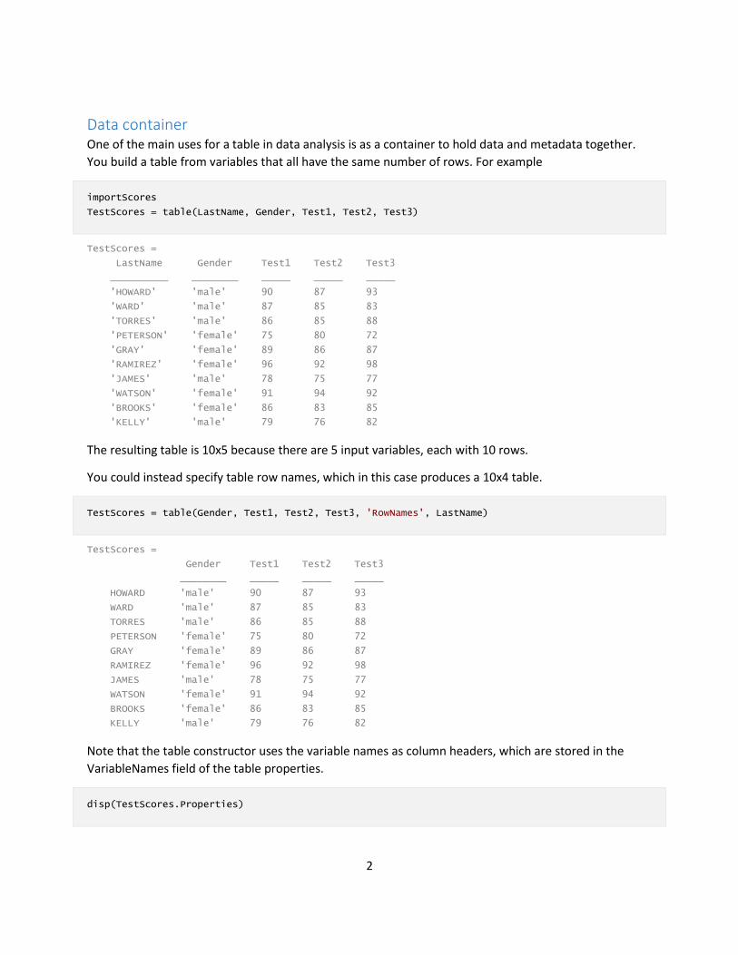
You can also put data arrays of compatible elements in a table.

AllTests = [Test1, Test2, Test3];

TestScores = table(Gender, AllTests, 'RowNames', LastName)

TestScores =

Gender AllTests

________ ______________

HOWARD 'male' 90 87 93

WARD 'male' 87 85 83

TORRES 'male' 86 85 88

PETERSON 'female' 75 80 72

GRAY 'female' 89 86 87

RAMIREZ 'female' 96 92 98

JAMES 'male' 78 75 77

WATSON 'female' 91 94 92

BROOKS 'female' 86 83 85

KELLY 'male' 79 76 82

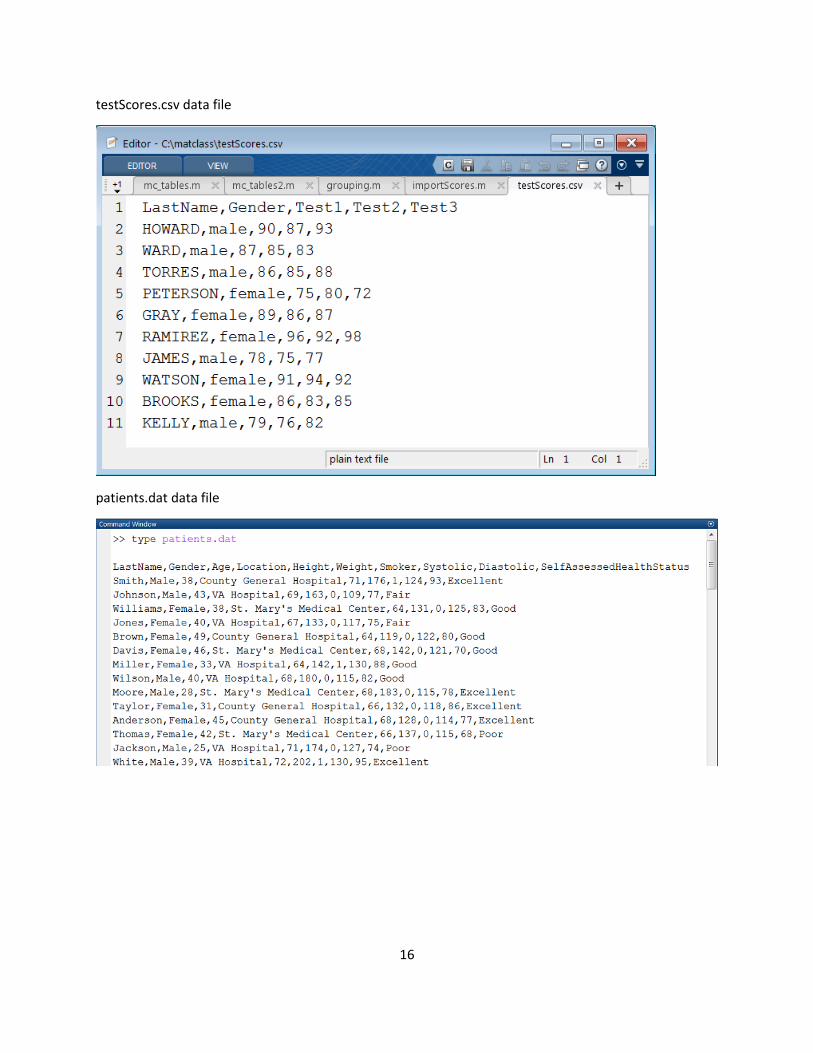
A not uncommon ASCII data file format would consist of a line of column headers followed by lines of

data with some character and some numeric columns.

There are several ways that you could read this file. You could parse it using textscan or fscanf as in

the custom importScores script, but this is tedious to design and would not be flexible for a varying

number of columns. It also leaves several variables to keep track of.

You could import the data into a structure, which works well in simple cases. However importdata

does not alway detect headers reliably, so you would need to parse the testdata field.

A = importdata('testScores.csv')

A =

data: [10x3 double]

textdata: {11x5 cell}

Even then, accessing the data by column header is a bit awkward.

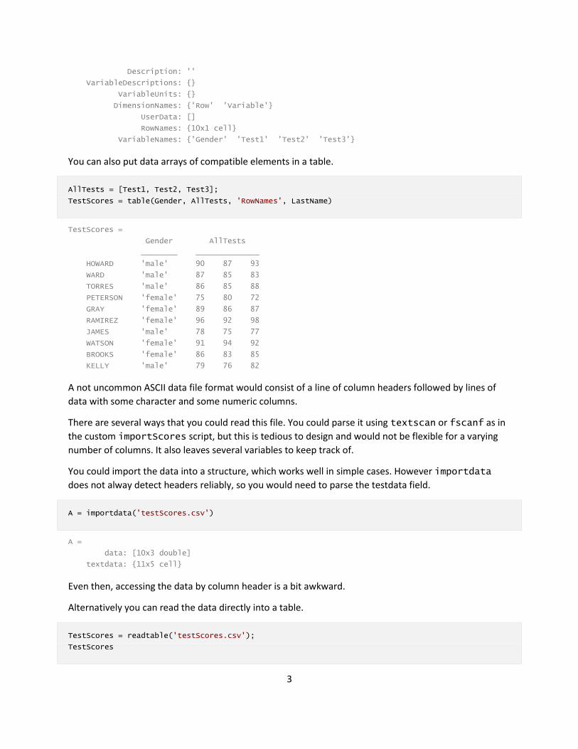
Alternatively you can read the data directly into a table.

TestScores = readtable('testScores.csv');

TestScores

4

TestScores =

LastName Gender Test1 Test2 Test3

__________ ________ _____ _____ _____

'HOWARD' 'male' 90 87 93

'WARD' 'male' 87 85 83

'TORRES' 'male' 86 85 88

'PETERSON' 'female' 75 80 72

'GRAY' 'female' 89 86 87

'RAMIREZ' 'female' 96 92 98

'JAMES' 'male' 78 75 77

'WATSON' 'female' 91 94 92

'BROOKS' 'female' 86 83 85

'KELLY' 'male' 79 76 82

The readtable function also supports many options about how to handle headers, missing values, and

selection ranges. The table makes it easy to work with one or more variables (columns).

disp(TestScores.Gender)

'male'

'male'

'male'

'female'

'female'

'female'

'male'

'female'

'female'

'male'

5

Computing with tables To operate on the table contents, you can index into the table.

T1Mean = mean(TestScores{:,3})

T1Mean =

85.7000

Note the curly braces for indexing. So far MATLAB uses curly braces only for tables and cell arrays.

Alternatively you can extract the data using column number, then apply the computation.

Test1 = TestScores{:,3};

T1Mean = mean(Test1)

T1Mean =

85.7000

Or you can use the column name

Test1 = TestScores{:,'Test1'};

T1Mean = mean(Test1)

T1Mean =

85.7000

Of course computing with the data by indexing into the table will have some overhead. If you will work

with the data more than once, it is probably best to extract the data into one or more simple variables.

Much of the usual function grammar can be extended and used with tables. For example to compute

the data means in the row direction:

average = mean(TestScores{:, {'Test1', 'Test2', 'Test3'}},2)

average =

90.0000

85.0000

86.3333

75.6667

87.3333

95.3333

76.6667

92.3333

84.6667

79.0000

You can add compatible length columns to the table and specify the column or variable name.

6

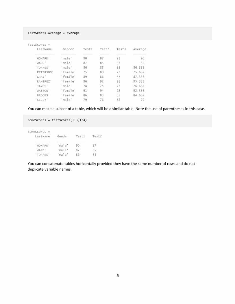
TestScores.Average = average

TestScores =

LastName Gender Test1 Test2 Test3 Average

__________ ________ _____ _____ _____ _______

'HOWARD' 'male' 90 87 93 90

'WARD' 'male' 87 85 83 85

'TORRES' 'male' 86 85 88 86.333

'PETERSON' 'female' 75 80 72 75.667

'GRAY' 'female' 89 86 87 87.333

'RAMIREZ' 'female' 96 92 98 95.333

'JAMES' 'male' 78 75 77 76.667

'WATSON' 'female' 91 94 92 92.333

'BROOKS' 'female' 86 83 85 84.667

'KELLY' 'male' 79 76 82 79

You can make a subset of a table, which will be a similar table. Note the use of parentheses in this case.

SomeScores = TestScores(1:3,1:4)

SomeScores =

LastName Gender Test1 Test2

________ ______ _____ _____

'HOWARD' 'male' 90 87

'WARD' 'male' 87 85

'TORRES' 'male' 86 85

You can concatenate tables horizontally provided they have the same number of rows and do not

duplicate variable names.

7

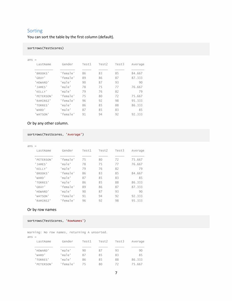
Sorting You can sort the table by the first column (default).

sortrows(TestScores)

ans =

LastName Gender Test1 Test2 Test3 Average

__________ ________ _____ _____ _____ _______

'BROOKS' 'female' 86 83 85 84.667

'GRAY' 'female' 89 86 87 87.333

'HOWARD' 'male' 90 87 93 90

'JAMES' 'male' 78 75 77 76.667

'KELLY' 'male' 79 76 82 79

'PETERSON' 'female' 75 80 72 75.667

'RAMIREZ' 'female' 96 92 98 95.333

'TORRES' 'male' 86 85 88 86.333

'WARD' 'male' 87 85 83 85

'WATSON' 'female' 91 94 92 92.333

Or by any other column.

sortrows(TestScores, 'Average')

ans =

LastName Gender Test1 Test2 Test3 Average

__________ ________ _____ _____ _____ _______

'PETERSON' 'female' 75 80 72 75.667

'JAMES' 'male' 78 75 77 76.667

'KELLY' 'male' 79 76 82 79

'BROOKS' 'female' 86 83 85 84.667

'WARD' 'male' 87 85 83 85

'TORRES' 'male' 86 85 88 86.333

'GRAY' 'female' 89 86 87 87.333

'HOWARD' 'male' 90 87 93 90

'WATSON' 'female' 91 94 92 92.333

'RAMIREZ' 'female' 96 92 98 95.333

Or by row names

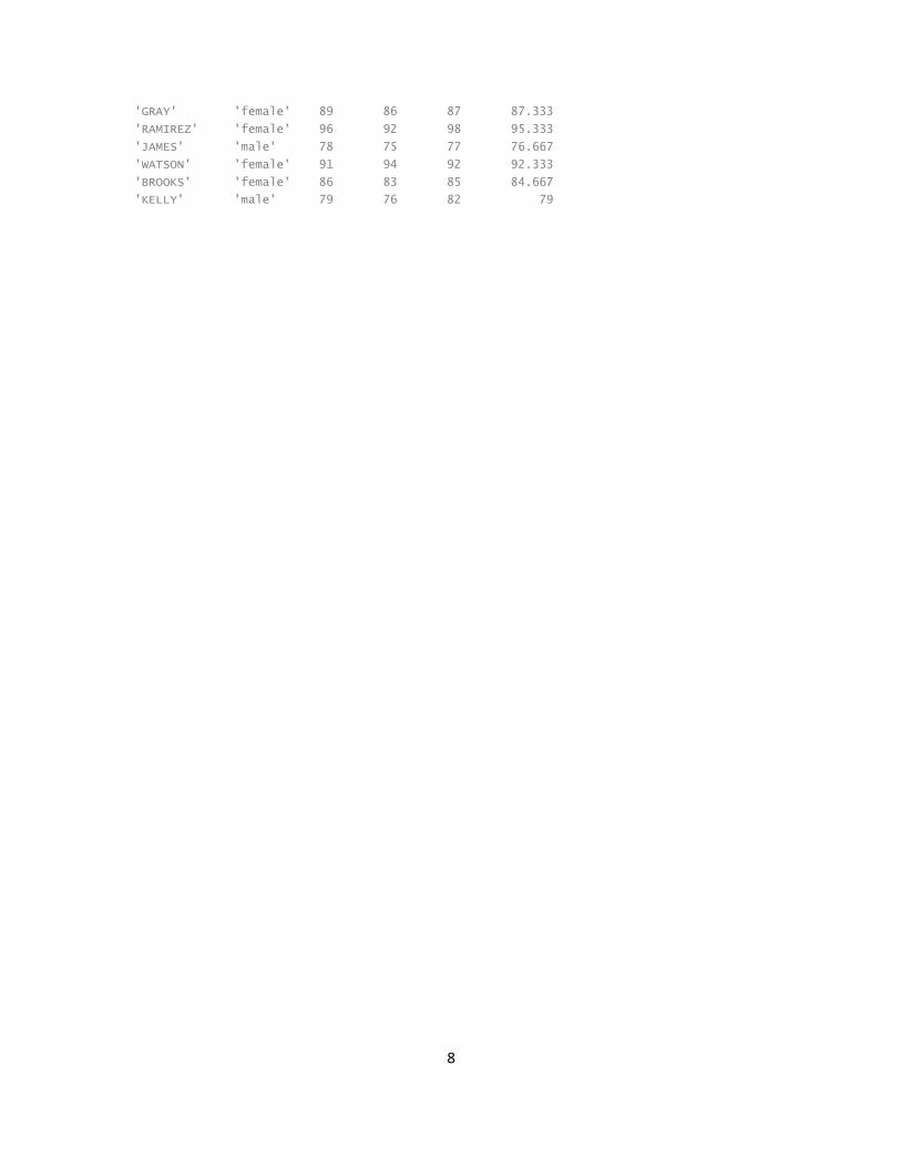
sortrows(TestScores, 'RowNames')

Warning: No row names, returning A unsorted.

ans =

LastName Gender Test1 Test2 Test3 Average

__________ ________ _____ _____ _____ _______

'HOWARD' 'male' 90 87 93 90

'WARD' 'male' 87 85 83 85

'TORRES' 'male' 86 85 88 86.333

'PETERSON' 'female' 75 80 72 75.667

8

'GRAY' 'female' 89 86 87 87.333

'RAMIREZ' 'female' 96 92 98 95.333

'JAMES' 'male' 78 75 77 76.667

'WATSON' 'female' 91 94 92 92.333

'BROOKS' 'female' 86 83 85 84.667

'KELLY' 'male' 79 76 82 79

9

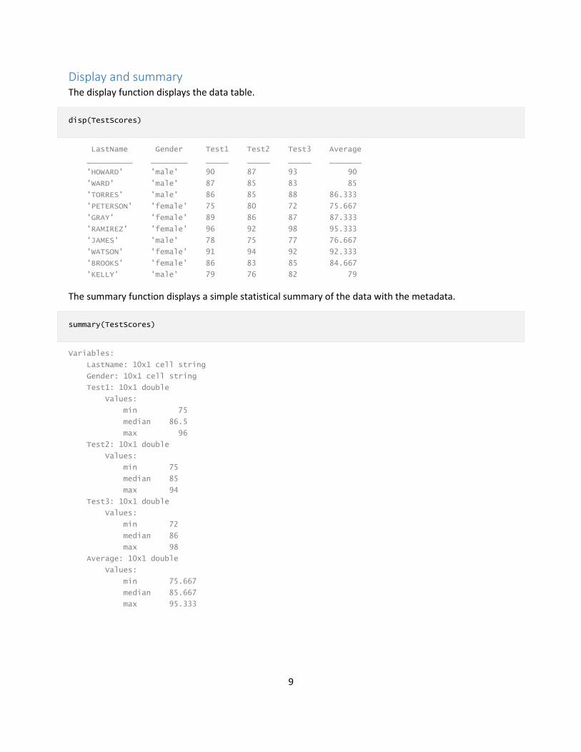
Display and summary The display function displays the data table.

disp(TestScores)

LastName Gender Test1 Test2 Test3 Average

__________ ________ _____ _____ _____ _______

'HOWARD' 'male' 90 87 93 90

'WARD' 'male' 87 85 83 85

'TORRES' 'male' 86 85 88 86.333

'PETERSON' 'female' 75 80 72 75.667

'GRAY' 'female' 89 86 87 87.333

'RAMIREZ' 'female' 96 92 98 95.333

'JAMES' 'male' 78 75 77 76.667

'WATSON' 'female' 91 94 92 92.333

'BROOKS' 'female' 86 83 85 84.667

'KELLY' 'male' 79 76 82 79

The summary function displays a simple statistical summary of the data with the metadata.

summary(TestScores)

Variables:

LastName: 10x1 cell string

Gender: 10x1 cell string

Test1: 10x1 double

Values:

min 75

median 86.5

max 96

Test2: 10x1 double

Values:

min 75

median 85

max 94

Test3: 10x1 double

Values:

min 72

median 86

max 98

Average: 10x1 double

Values:

min 75.667

median 85.667

max 95.333

10

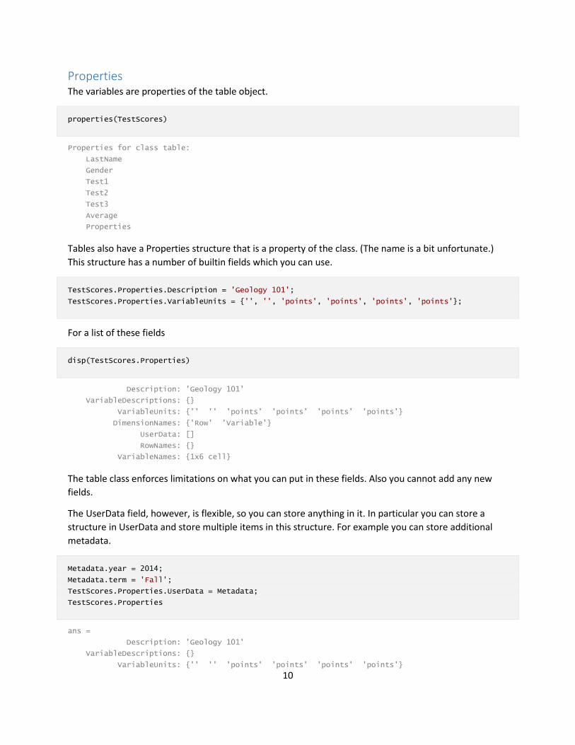
Properties The variables are properties of the table object.

properties(TestScores)

Properties for class table:

LastName

Gender

Test1

Test2

Test3

Average

Properties

Tables also have a Properties structure that is a property of the class. (The name is a bit unfortunate.)

This structure has a number of builtin fields which you can use.

TestScores.Properties.Description = 'Geology 101';

TestScores.Properties.VariableUnits = {'', '', 'points', 'points', 'points', 'points'};

For a list of these fields

disp(TestScores.Properties)

Description: 'Geology 101'

VariableDescriptions: {}

VariableUnits: {'' '' 'points' 'points' 'points' 'points'}

DimensionNames: {'Row' 'Variable'}

UserData: []

RowNames: {}

VariableNames: {1x6 cell}

The table class enforces limitations on what you can put in these fields. Also you cannot add any new

fields.

The UserData field, however, is flexible, so you can store anything in it. In particular you can store a

structure in UserData and store multiple items in this structure. For example you can store additional

metadata.

Metadata.year = 2014;

Metadata.term = 'Fall';

TestScores.Properties.UserData = Metadata;

TestScores.Properties

ans =

Description: 'Geology 101'

VariableDescriptions: {}

VariableUnits: {'' '' 'points' 'points' 'points' 'points'}

11

DimensionNames: {'Row' 'Variable'}

UserData: [1x1 struct]

RowNames: {}

VariableNames: {1x6 cell}

and

TestScores.Properties.UserData

ans =

year: 2014

term: 'Fall'

You can change a variable name through the properties.

TestScores.Properties.VariableNames{'Gender'} = 'Sex'

TestScores =

LastName Sex Test1 Test2 Test3 Average

__________ ________ _____ _____ _____ _______

'HOWARD' 'male' 90 87 93 90

'WARD' 'male' 87 85 83 85

'TORRES' 'male' 86 85 88 86.333

'PETERSON' 'female' 75 80 72 75.667

'GRAY' 'female' 89 86 87 87.333

'RAMIREZ' 'female' 96 92 98 95.333

'JAMES' 'male' 78 75 77 76.667

'WATSON' 'female' 91 94 92 92.333

'BROOKS' 'female' 86 83 85 84.667

'KELLY' 'male' 79 76 82 79

Search the documentation for Table Properties to see more information on properties. You cannot add

new properties to a table.

12

Methods The table public methods are oriented toward database and array operations.

methods(TestScores)

Methods for class table:

cat numel table

height outerjoin union

horzcat rowfun unique

innerjoin setdiff unstack

intersect setxor varfun

isempty size vertcat

ismember sortrows width

ismissing stack write

join standardizeMissing

ndims summary

13

Style Use upper case for the first letter of a table name. If the name is a compound word, use upper

case for the first letter of each word.

Use meaningful names for variables and UserData fields.

In general make table variable names valid MATLAB names.

Use a consistent case for the first letter of each variable name.

If there is no meaningful order for variables, put them in alphabetical order by variable name.

If there is no meaningful order for rows, put them in alphabetical order by row names.

Avoid using variables that have more than two dimensions.

Other considerations MathWorks recommends that you use tables rather than datasets.

A structure is more flexible than a table but offers less data integrity.

Review of table fundamentals A table is most useful for storing column-oriented data where the columns (variables) have

different data types.

It is a class with properties and methods.

Its public properties are the data variables and a structure unfortunately named Properties.

The Properties structure has non-extendable fields that are useful for metadata. One of the

fields of Properties is a structure named UserData that you can use for arbitrary contents.

Most of its methods support database and logical set operations. It also has overloads for many

computational functions.

It supports normal indexing for data extraction or replacement.

There is an import function readtable that is useful but a bit limited. You can also use the

Import Data Wizard.

14

Exercises 1.

Display the test scores for Gray.

Try multiple ways to select the data.

2.

Make a table named "Study" from patients.dat

Remove the "Location" variable.

How big is the table?

Display the first 6 rows and columns of the table.

Summarize the table.

Add unit properties to the variables.

3.

The body mass index (BMI) is computed as weight divided by height squared. The units are kilograms

per square meter. 0.454 kg equals one pound. 0.0254 m equals one inch. Compute BMI for the data.

Add the result to the table.

4.

Compare average BMI for males and females.

Plot weight vs. height for males and females.

15

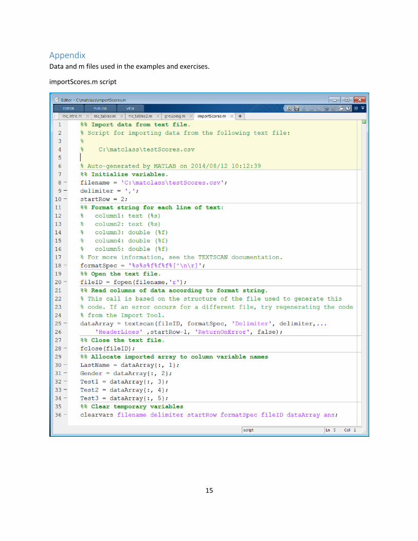
Appendix Data and m files used in the examples and exercises.

importScores.m script

16

testScores.csv data file

patients.dat data file