Embed Size (px)
Citation preview

- 1 - | P a g e
MATLAB: SIGNAL PROCESSING

- 2 - | P a g e
CONTENT
Chapter No. Title Page No. Chapter 1 Introduction 3 Chapter 2 Arithmetic Operations 4-6 Chapter 3 Trigonometric Calculations 7-9
Chapter 4 Matrices 10-13 Chapter 5 Features of Matrices 14-18 Chapter 6 2-D Plot 19-20 Chapter 7 2-D Plot Designing 21-27
Chapter 8 2-D Plot Fig. & Subplot 28-32 Chapter 9 3-D Plot 33-35
Chapter 10 Input Values 36-39

- 3 - | P a g e
CHAPTER 1
INTRODUCTION
1.1 MATLAB an Introduction
MATLAB is a language of technical computing.
MATLAB (matrix laboratory) is a multi-paradigm numerical computing environment and
fourth-generation programming language.
A proprietary programming language developed by MathWorks, MATLAB allows matrix
manipulations, plotting of functions and data, implementation of algorithms, creation of user
interfaces, and interfacing with programs written in other languages, including C, C++, Java,
Fortran and Python.
In 2004, MATLAB had around one million users across industry and academia.
MATLAB users come from various backgrounds of engineering, science, and economics.
Millions of engineers and scientists worldwide use MATLAB® to analyze and design the
systems and products transforming our world.
MATLAB is in automobile active safety systems, interplanetary spacecraft, health monitoring
devices, smart power grids, and LTE cellular networks.
It is used for machine learning, signal processing, image processing, computer vision,
communications, computational finance, control design, robotics, and much more.
The MATLAB platform is optimized for solving engineering and scientific problems.
The matrix-based MATLAB language is the world’s most natural way to express computational
mathematics.
Built-in graphics make it easy to visualize and gain insights from data.
A vast library of prebuilt toolboxes lets you get started right away with algorithms essential to
your domain.
The desktop environment invites experimentation, exploration, and discovery.
These MATLAB tools and capabilities are all rigorously tested and designed to work together.
MATLAB helps you take your ideas beyond the desktop. You can run your analyses on larger
data sets and scale up to clusters and clouds.

- 4 - | P a g e
CHAPTER 2
ARITHMETIC OPERATION
Variable Assignment
In MATLAB we need to simply assign the variable with the corresponding values and calculate the results. For example let’s take a=1 >> a=1 a = 1 For example let’s take b=2 >> b=2 b = 2 So we can easily calculate c=a+b >> c=a+b c = 3 Note: we don’t need to specify data type or put traditional header files to assign a value to variable in MATLAB.
Practice set 1
Question 1: If a=2000, b=3000 find (a^2)+2*a*b+(b^2). Solution : >> a=2000 a = 2000
- 5 - | P a g e
>> b=3000 b = 3000 >> (a^2)+2*a*b+(b^2) ans = 25000000
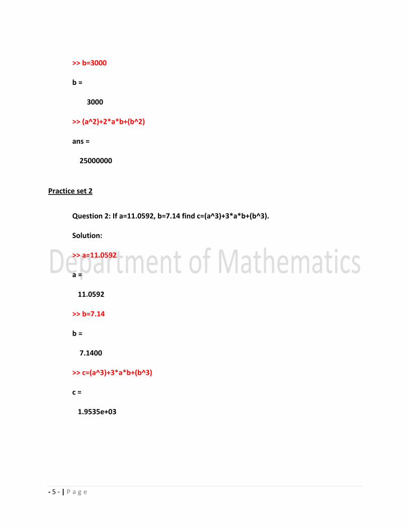
Practice set 2
Question 2: If a=11.0592, b=7.14 find c=(a^3)+3*a*b+(b^3). Solution: >> a=11.0592 a = 11.0592 >> b=7.14 b = 7.1400 >> c=(a^3)+3*a*b+(b^3) c = 1.9535e+03

- 6 - | P a g e
Practice set 3
Question 3: If a=12596, b=9.1463, c=1000 find c=(a+b+c)^3. Solution: >> a=12596 a = 12596 >> b=9.1463 b = 9.1463 >> c=1000 c = 1000 >> c=(a+b+c)^3 c = 2.5183e+12 Assignments If a=2015.205, b=658.365 , c=987.695 then find 1. d= (a+b)/c 2. e= (a-b)/c 3. f= (a*b)/c 4. g= ((a*b)/c)+( (a+b)/c)

- 7 - | P a g e
CHAPTER 3
Trigonometric Calculations
1.1 Trigonometric Calculations
In MATLAB we just need to call the name of trigonometric functions and its values will
be calculated because of inbuilt toolbox.
For example
>>sin(0)
ans =
0
>>sin(pi/6)
ans =
0.5000
>>cos(pi/4)
ans =
0.7071
>>tan(pi/4)
ans =
1.0000
Practice set 1
Question 1: Find the value of sin(pi/2)+cos(pi/2)+tan(pi/2).
Solution :

- 8 - | P a g e
>>sin(pi/2)+cos(pi/2)+tan(pi/2)
ans =
1.6331e+16
Practice set 2
Question 2: Find the value of sin(pi/2)-cos(pi/4)+tan(pi/2).
Solution:
>>sin(pi/2)-cos(pi/4)+tan(pi/2)
ans =
1.6331e+16
Practice set 3
Question 3: If a=pi/2 , b=pi/4, c=pi/6 find sin(a)+ cos(b)*tan(c).
Solution:
>> a=pi/2
a =
1.5708
>> b=pi/4
b =
0.7854
>> c=pi/6

- 9 - | P a g e
c =
0.5236
>>sin(a)+ cos(b)*tan(c)
ans =
1.4082
Assignments
If a=pi/6, b=pi/4 , c=pi/2 then find
5. d= sin(a+b)
6. e= cos(a-b)
7. f= sin(a+b)+ cos(a-b)
8. g= sin(a)+cos(b)+tan(c)

- 10 - | P a g e
CHAPTER-4
MATRICES 1.1 Matrix Creation
In MATLAB it’s very easy to create a matrix.
Example 1 :We want to create a 2*2 matrix with elements [2 3; 4 5] then we will
write
>> a=[2 3;4 5]
a =
2 3
4 5
Example 2 :We want to create a 3*3 matrix with elements [1 2 3; 4 5 6; 7 8 9] then
we will write
>>b=[1 2 3; 4 5 6; 7 8 9]
b =
1 2 3
4 5 6
7 8 9
Example 3 :We want to create a 3*3 matrix with elements [4 2 5; 4 8 6; 7 8 7]
then we will write
>>c=[4 2 5; 4 8 6; 7 8 7]
c =
4 2 5
4 8 6
7 8 7
1.2 Matrix Arithmetic
We can do addition, subtraction, multiplication operations for the matrices.
Example 1 : Create two matrices of 2*2 with elements a=[2 3; 4 5] and b= [3 5; 6 7] ,
add them and find the value of c=a+b.
>> a=[2 3; 4 5]

- 11 - | P a g e
a =
2 3
4 5
>> b= [3 5; 6 7]
b =
3 5
6 7
>> c=a+b
c =
5 8
10 12
Example 2 : Create two matrices of 3*3 with elements a=[1 2 3; 4 5 6; 7 8 9] and b= [3
5 7; 6 7 7; 9 10 12] , subtract them and find the value of c=a-b.
>> a=[1 2 3; 4 5 6; 7 8 9]
a =
1 2 3
4 5 6
7 8 9
>> b= [3 5 7; 6 7 7; 9 10 12]
b =
3 5 7
6 7 7
9 10 12
>> c=a-b

- 12 - | P a g e
c =
-2 -3 -4
-2 -2 -1
-2 -2 -3
Example 3 : Create two matrices of 3*3 with elements a=[10 20 30; 40 50 60; 70 80 90]
and b= [30 50 71; 64 78 79; 94 10 12] , multiply them and find the value of c=a*b.
>> a=[10 20 30; 40 50 60; 70 80 90]
a =
10 20 30
40 50 60
70 80 90
>> b= [30 50 71; 64 78 79; 94 10 12]
b =
30 50 71
64 78 79
94 10 12
>> c=a*b
c =
4400 2360 2650
10040 6500 7510
15680 10640 12370

- 13 - | P a g e
Assignments
If a=[10 20 30; 40 50 60; 70 80 90], b= [3 5 7; 6 7 7; 9 10 12], c=[1 2 3; 4 5 6; 7 8 9] then
find
1. d= a+b-c
2. e= (a/b)*c
3. f= (a+b)+(a-b)+(a*b)+(a/d)
4. g= a+b-c+(b/a)+(c/b)

- 14 - | P a g e
CHAPTER 5
FEATURES OF MATRICES
1.1 Transpose: Rows as columns and columns as rows.
Example 1 :Find the transpose of matrix A= [4 2 5; 4 8 6; 7 8 7]
>> A= [4 2 5; 4 8 6; 7 8 7]
A =
4 2 5
4 8 6
7 8 7
The symbol of transpose is ( ‘ )
>> B=A'
B =
4 4 7
2 8 8
5 6 7
Example 2 :Find the transpose of matrix B= [1 2 3; 4 5 6; 7 8 9]
>> B= [1 2 3; 4 5 6; 7 8 9]
B =
1 2 3
4 5 6
7 8 9
>> C=B'
C =
1 4 7
2 5 8
3 6 9
- 15 - | P a g e
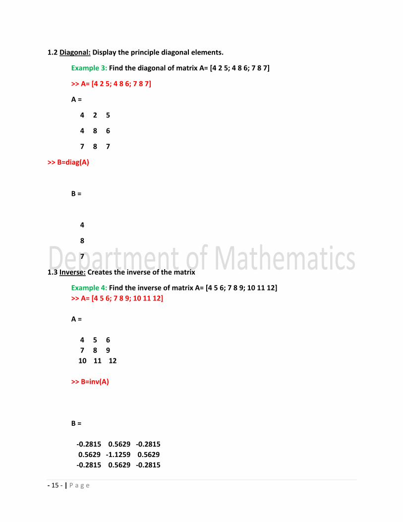
1.2 Diagonal: Display the principle diagonal elements.
Example 3: Find the diagonal of matrix A= [4 2 5; 4 8 6; 7 8 7]
>> A= [4 2 5; 4 8 6; 7 8 7]
A =
4 2 5
4 8 6
7 8 7
>> B=diag(A)
B =
4
8
7
1.3 Inverse: Creates the inverse of the matrix
Example 4: Find the inverse of matrix A= [4 5 6; 7 8 9; 10 11 12]
>> A= [4 5 6; 7 8 9; 10 11 12]
A =
4 5 6
7 8 9
10 11 12
>> B=inv(A)
B =
-0.2815 0.5629 -0.2815
0.5629 -1.1259 0.5629
-0.2815 0.5629 -0.2815

- 16 - | P a g e
1.4 Identity Matrix: Matrix with principle diagonal element as unity.
Example 5: Create an identity matrix of 3*3 elements
>> A= eye(3,3)
>> A= eye(3,3)
A =
1 0 0
0 1 0
0 0 1
Example 6: Create an identity matrix of 4*4 elements
>> A= eye(4,4)
A =
1 0 0 0
0 1 0 0
0 0 1 0
0 0 0 1
1.5 Unit Matrix: Matrix with all elements as unity.
Example 6: Create an unit matrix of 3*3 elements
>> A= ones(3,3)
>> A= ones(3,3)
A =
1 1 1
1 1 1
1 1 1

- 17 - | P a g e
Example 7: Create an unit matrix of 4*4 elements
>> A= ones(4,4)
A =
1 1 1 1
1 1 1 1
1 1 1 1
1 1 1 1
1.6 Magic Matrix: Matrix with all elements sum as same number.
Example 8: Create a magic matrix of 3*3 elements
>> A= magic(3)
A =
8 1 6
3 5 7
4 9 2
Example 9: Create a magic matrix of 4*4 elements
>> A= magic(4)
A =
16 2 3 13
5 11 10 8
9 7 6 12
4 14 15 1
1.7 Determinant of a Matrix: Calculates the determinant value of a matrix.
Example 10: Calculate the determinant value of a matrix A= [4 5 6; 7 8 9; 10 11 12] .
>> A= [4 5 6; 7 8 9; 10 11 12]

- 18 - | P a g e
A =
4 5 6
7 8 9
10 11 12
>> B=det(A)
B =
1.0658e-14
Example 11: Calculate the determinant value of a matrix A= [1 2 3; 7 8 9; 1 1 1] .
>>A= [1 2 3; 7 8 9; 1 1 1]
A =
1 2 3
7 8 9
1 1 1
Assignments
If a=[10 20 30; 40 50 60; 70 80 90], b= [3 5 7; 6 7 7; 9 10 12], c=[1 2 3; 4 5 6; 7 8 9] then
find
1. Determinant of a,b,c
2. Find inverse of a,b,c
3. Create a unity matrix and identity matrix of 3*3 elements.
- 19 - | P a g e
CHAPTER 6
2D-PLOT
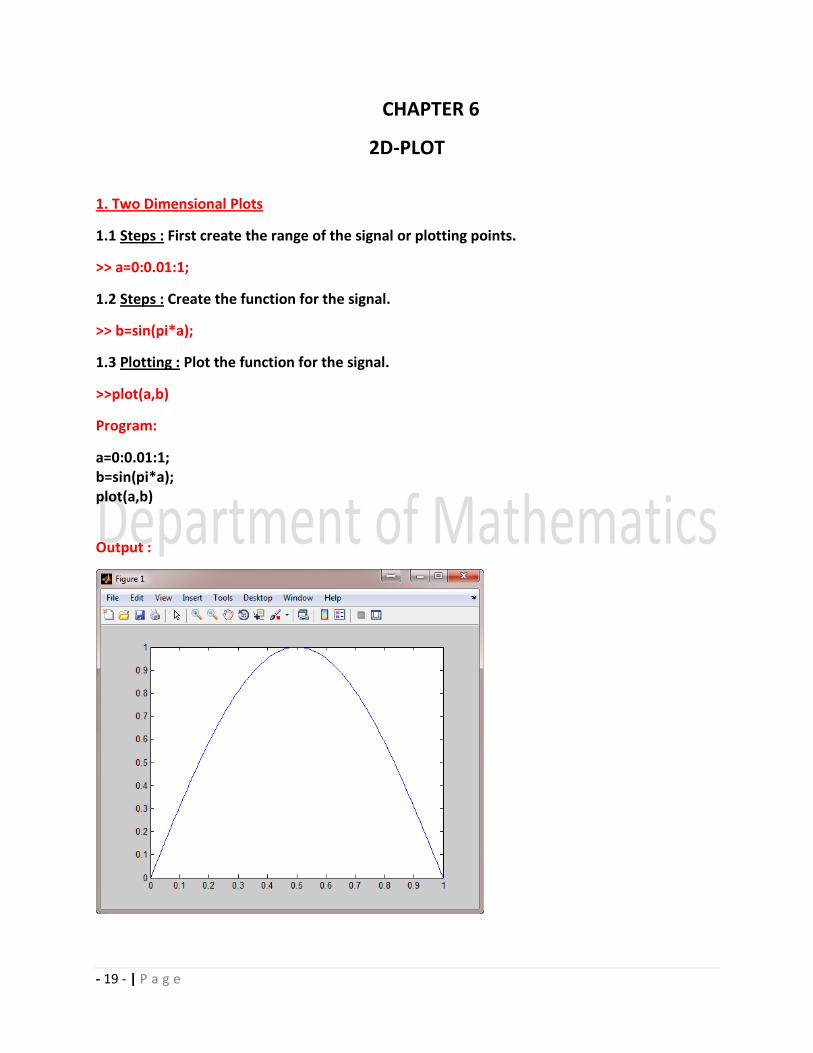
1. Two Dimensional Plots
1.1 Steps : First create the range of the signal or plotting points.
>> a=0:0.01:1;
1.2 Steps : Create the function for the signal.
>> b=sin(pi*a);
1.3 Plotting : Plot the function for the signal.
>>plot(a,b)
Program:
a=0:0.01:1; b=sin(pi*a); plot(a,b)
Output :

- 20 - | P a g e
Example 1: Create a sine wave with range 0 to 1 and the phase shift of (2*pi).
Program:
a=0:0.01:1; b=sin(2*pi*a); plot(a,b)
Output :
Note :Commands for different trigonometric functions
1. SINE: sin 4. COSEC: csc
2. COSINE: cos5. SEC: sec
3. TAN: tan 6. COT: cot
Assignments
1. Create a sine wave with range 0 to 1 and the phase shift of (2*pi).
2. Create a cosine wave with range 0 to 1 and the phase shift of (3*pi).
3. Create a tan wave with range 0 to 1 and the phase shift of (5*pi).
4. Create a cosec wave with range 0 to 2 and the phase shift of (2*pi).
5. Create a sec wave with range 0 to 3 and the phase shift of (2*pi).
6. Create a cot wave with range 0 to 2 and the phase shift of (5*pi).

- 21 - | P a g e
7. CHAPTER 7
2D-PLOT-DESIGNING
1. LABEL
1.1 Steps : First create the range of the signal or plotting points.
>> a=0:0.01:1;
1.2 Steps : Create the function for the signal.
>> b=sin(2*pi*a);
1.3 Plotting : Plot the function for the signal.
>>plot(a,b)
1.4 Steps : Create the label of x axis.
>>xlabel(‘X Axis’)
1.5 Steps : Create the label of y axis.
>>ylabel(‘Y Axis’)
Program:
a=0:0.01:1; b=sin(2*pi*a); plot(a,b) xlabel('X Axis') ylabel('Y Axis')
Output :
- 22 - | P a g e
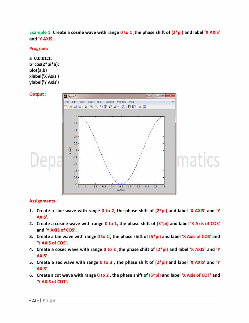
Example 1: Create a cosine wave with range 0 to 1 ,the phase shift of (2*pi) and label ‘X AXIS’
and ‘Y AXIS’.
Program:
a=0:0.01:1; b=cos(2*pi*a); plot(a,b) xlabel('X Axis') ylabel('Y Axis') Output :
Assignments
1. Create a sine wave with range 0 to 2, the phase shift of (2*pi) and label ‘X AXIS’ and ‘Y
AXIS’.
2. Create a cosine wave with range 0 to 1, the phase shift of (3*pi) and label ‘X Axis of COS’
and ‘Y AXIS of COS’.
3. Create a tan wave with range 0 to 1 , the phase shift of (5*pi) and label ‘X Axis of COS’ and
‘Y AXIS of COS’.
4. Create a cosec wave with range 0 to 2 ,the phase shift of (2*pi) and label ‘X AXIS’ and ‘Y
AXIS’.
5. Create a sec wave with range 0 to 3 , the phase shift of (2*pi) and label ‘X AXIS’ and ‘Y
AXIS’.
6. Create a cot wave with range 0 to 2 , the phase shift of (5*pi) and label ‘X Axis of COT’ and
‘Y AXIS of COT’.

- 23 - | P a g e
2. TITLE
1.1 Steps : First create the range of the signal or plotting points.
>> a=0:0.01:1;
1.2 Steps : Create the function for the signal.
>> b=sin(2*pi*a);
1.3 Plotting : Plot the function for the signal.
>>plot(a,b)
1.4 Steps : Create the label of x axis.
>>xlabel(‘X Axis’)
1.5 Steps : Create the label of y axis.
>>ylabel(‘Y Axis’)
1.6 Steps : Create the TITLE of wave.
>>title(‘SIN Wave’)
Program:
a=0:0.01:1; b=sin(2*pi*a); plot(a,b) xlabel('X Axis') ylabel('Y Axis') title(‘SIN Wave’) Output :

- 24 - | P a g e
Example 2: Create a cosine wave with range 0 to 1 ,the phase shift of (2*pi) , label ‘X AXIS’ , ‘Y
AXIS’ and title ‘Cos Wave’.
Program:
a=0:0.01:1; b=cos(2*pi*a); plot(a,b) xlabel('X Axis') ylabel('Y Axis') title(‘Cos Wave’)
Output :
3. LEGEND
1.1 Steps : First create the range of the signal or plotting points.
>> a=0:0.01:1;
1.2 Steps : Create the function for the signal.
>> b=sin(2*pi*a);
1.3 Plotting : Plot the function for the signal.
>>plot(a,b)
1.4 Steps : Create the label of x axis.

- 25 - | P a g e
>>xlabel(‘X Axis’)
1.5 Steps : Create the label of y axis.
>>ylabel(‘Y Axis’)
1.6 Steps : Create the TITLE of wave.
>>title(‘SIN Wave’)
1.7 Steps : Create the LEGEND of wave.
>>legend(‘SIN Wave’)
Program:
a=0:0.01:1; b=sin(2*pi*a); plot(a,b) xlabel('X Axis') ylabel('Y Axis') title(‘SIN Wave’) legend(‘SIN Wave’) Output:

- 26 - | P a g e
Example 3: Create a cosine wave with range 0 to 1 ,the phase shift of (2*pi) , label ‘X AXIS’ , ‘Y
AXIS’ ,title ‘Cos Wave’ and legend (‘COS Wave’).
Program:
a=0:0.01:1; b=cos(2*pi*a); plot(a,b) xlabel('X Axis') ylabel('Y Axis') title(‘Cos Wave’) legend(‘Cos Wave’)
Output :
Assignments
1. Create a sine wave and cosine wave with range 0 to 1 and the phase shift of (2*pi)
,add them (sin+cos) give label and titles.
Label : X Axis,YAxis
Title= Sin+Cos
Legend = Sin+Cos
- 27 - | P a g e
2. Create a sine wave and cosine wave with range 0 to 1 and the phase shift of (2*pi)
and subtract them (sin-cos) give label and titles.
Label : X Axis,YAxis
Title= Sin-Cos
Legend = Sin-Cos
3. Create a cosine wave and tan wave with range 0 to 1 and the phase shift of (3*pi)
and add them (cos+tan) give label and titles.
Label : X Axis,YAxis
Title= Cos+Tan
Legend = Cos+Tan
4. Create a cosine wave and tan wave with range 0 to 1 and the phase shift of (3*pi)
and subtract them (cos-tan) give label and titles.
Label : X Axis,YAxis
Title= Cos-Tan
Legend = Cos-Tan
5. Create a tan wave and cot wave with range 0 to 1 and the phase shift of (5*pi) and
add them (tan+cot) give label and titles.
Label : X Axis,YAxis
Title= Tan+Cot
Legend = Tan+Cot
6. Create a tan wave and cot wave with range 0 to 1 and the phase shift of (5*pi) and
subtract them (tan-cot) give label and titles.
Label : X Axis,YAxis
Title= Tan+Cot
Legend = Tan+Cot
7. Create a cot wave and cosec wave with range 0 to 1 and the phase shift of (5*pi)
and add them (cot+csc) give label and titles.
Label : X Axis,YAxis
Title= Cot+Cosec
Legend = Cot+Cosec
8. Create a cot wave and cosec wave with range 0 to 1 and the phase shift of (7*pi)
and subtract them (cot-csc) give label and titles.
Label : X Axis,YAxis
Title= Cot-Cosec
Legend = Cot-Cosec

- 28 - | P a g e
CHAPTER 8
2D-PLOT-Fig. & Subplot
1. Figure Plot
1.1 Step: First create the program for sine function.
a=0:0.01:1; b=sin(2*pi*a); plot(a,b) xlabel('X Axis') ylabel('Y Axis')
1.2 Step :Write the program for cos wave.
a=0:0.01:1; b=cos(2*pi*a); plot(a,b) xlabel('X Axis') ylabel('Y Axis')

- 29 - | P a g e
1.4 Step : Combine the codes.
a=0:0.01:1; b=sin(2*pi*a); c=cos(2*pi*a); figure(1) plot(a,b) xlabel('X Axis') ylabel('Y Axis') figure(2) plot(a,c) xlabel('X Axis') ylabel('Y Axis')
Output :
1.4 Step : Add the title and legend.
a=0:0.01:1; b=sin(2*pi*a); c=cos(2*pi*a); figure(1) plot(a,b) xlabel('X Axis') ylabel('Y Axis') title(‘Sin Wave’) legend(‘Sin Wave’) figure(2) plot(a,c) xlabel('X Axis')
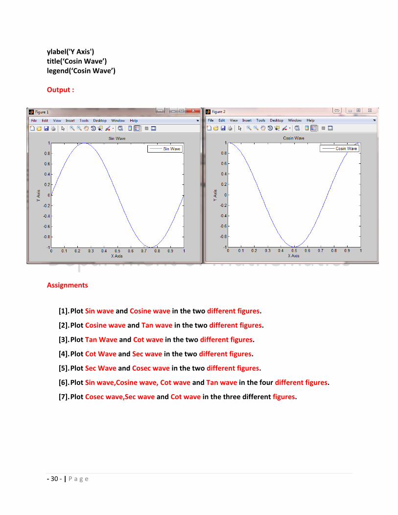
- 30 - | P a g e
ylabel('Y Axis') title(‘Cosin Wave’) legend(‘Cosin Wave’) Output :
Assignments
[1]. Plot Sin wave and Cosine wave in the two different figures.
[2]. Plot Cosine wave and Tan wave in the two different figures.
[3]. Plot Tan Wave and Cot wave in the two different figures.
[4]. Plot Cot Wave and Sec wave in the two different figures.
[5]. Plot Sec Wave and Cosec wave in the two different figures.
[6]. Plot Sin wave,Cosine wave, Cot wave and Tan wave in the four different figures.
[7]. Plot Cosec wave,Sec wave and Cot wave in the three different figures.

- 31 - | P a g e
2. Sub Plot
1.1 Step: First create the program for sine function.
a=0:0.01:1; b=sin(2*pi*a); plot(a,b) xlabel('X Axis') ylabel('Y Axis')
1.2 Step :Write the program for cos wave.
a=0:0.01:1; b=cos(2*pi*a); plot(a,b) xlabel('X Axis') ylabel('Y Axis')
1.4 Step : Combine the codes.
a=0:0.01:1; b=sin(2*pi*a); c=cos(2*pi*a); subplot(1,2,1) plot(a,b) xlabel('X Axis') ylabel('Y Axis') subplot(1,2,2) plot(a,c) xlabel('X Axis') ylabel('Y Axis')

- 32 - | P a g e
1.4 Step : Add the title and legend.
a=0:0.01:1; b=sin(2*pi*a); c=cos(2*pi*a); subplot(1,2,1) plot(a,b) xlabel('X Axis') ylabel('Y Axis') title(‘Sin Wave’) legend(‘Sin Wave’) subplot(1,2,2) plot(a,c) xlabel('X Axis') ylabel('Y Axis') title(‘Cosin Wave’) legend(‘Cosin Wave’)
Assignments
1. Subplot Sin wave and Cosine wave.
2. Subplot Cosine wave and Tan wave.
3. Subplot Tan Wave and Cot wave.
4. Subplot Cot Wave and Sec wave.
5. Subplot Sec Wave and Cosec wave.
6. Subplot Sin wave,Cosine wave, Cot wave and Tan wave.
7. Subplot Cosec wave,Sec wave and Cot wave.

- 33 - | P a g e
CHAPTER 9
3D PLOT
3D PLOT
1.1 Step: First create the program for sine function.
a=0:0.01:1; b=sin(2*pi*a); plot(a,b) xlabel('X Axis') ylabel('Y Axis') OUTPUT

- 34 - | P a g e
1.2 Step :Change the program to get 3D plot.
a=0:0.01:1; b=sin(2*pi*a); c=b’*b; surf(c) xlabel('X Axis') ylabel('Y Axis') zlabel('Z Axis') legend(‘Sin 3D Plot’) OUTPUT
- 35 - | P a g e
Assignments
3-D Figure Plot
1. Plot 3-D Sin wave and Cosine wave in the two different figures.
2. Plot 3-D Cosine wave and Tan wave in the two different figures.
3. Plot 3-D Tan Wave and Cot wave in the two different figures.
4. Plot 3-DCot Wave and Sec wave in the two different figures.
5. Plot 3-DSec Wave and Cosec wave in the two different figures.
6. Plot 3-DSin wave,Cosine wave, Cot wave and Tan wave in the four different figures.
7. Plot 3-DCosec wave,Sec wave and Cot wave in the three different figures.
8. Subplot Sin wave and Cosine wave.
9. Subplot Cosine wave and Tan wave.
3-D Subplot
1. Subplot 3-D Tan Wave and Cot wave.
2. Subplot 3-D Cot Wave and Sec wave.
3. Subplot 3-D Sec Wave and Cosec wave.
4. Subplot 3-D Sin wave,Cosine wave, Cot wave and Tan wave.
5. Subplot 3-DCosec wave,Sec wave and Cot wave
- 36 - | P a g e
CHAPTER 10
INPUT VALUES
SINGLE INPUT VALUES (2 D)
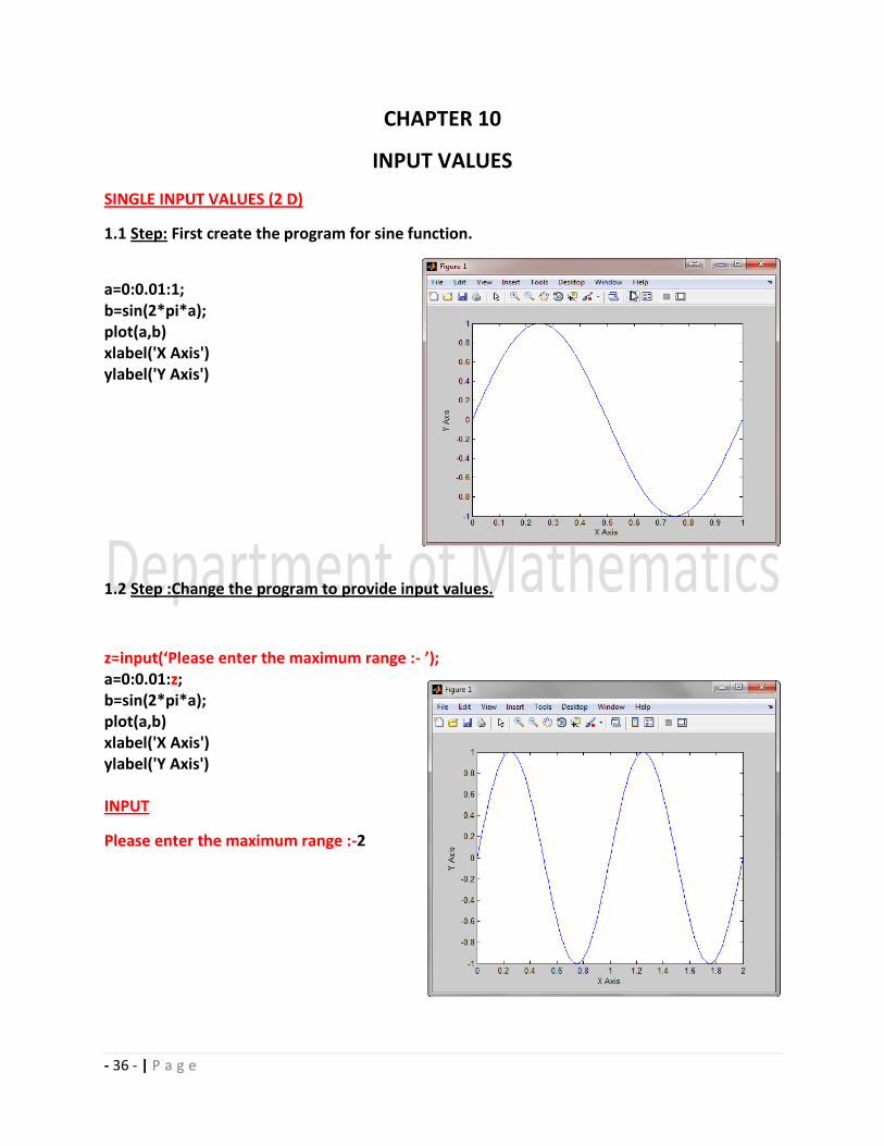
1.1 Step: First create the program for sine function.
a=0:0.01:1; b=sin(2*pi*a); plot(a,b) xlabel('X Axis') ylabel('Y Axis')
1.2 Step :Change the program to provide input values.
z=input(‘Please enter the maximum range :- ’); a=0:0.01:z; b=sin(2*pi*a); plot(a,b) xlabel('X Axis') ylabel('Y Axis') INPUT
Please enter the maximum range :-2

- 37 - | P a g e
DOUBLE INPUT VALUES (2 D)
1.1 Step: First create the program for sine function.
a=0:0.01:1; b=sin(2*pi*a); plot(a,b) xlabel('X Axis') ylabel('Y Axis')
1.2 Step :Change the program to provide input values.
y=input(‘Please enter the maximum range :- ’); z=input(‘Please enter the minimum range :- ’); a=z:0.01:y; b=sin(2*pi*a); plot(a,b) xlabel('X Axis') ylabel('Y Axis') INPUT
Please enter the maximum range: - 2
Please enter the minimum range: - 2

- 38 - | P a g e
INPUT VALUES (3 D)
1.1 Step: First create the program for sine function.
a=0:0.01:1; b=sin(2*pi*a); plot(a,b) xlabel('X Axis') ylabel('Y Axis') OUTPUT
1.2 Step :Change the program to provide input values.
z=input(‘Please enter the maximum range :- ’); y=input(‘Please enter the minimum range :- ’); a=y:0.01:z; b=sin(2*pi*a); c=b’*b; surf(c) xlabel('X Axis') ylabel('Y Axis') zlabel('Z Axis') legend(‘Sin 3D Plot’) INPUT
Please enter the maximum range :-2
Please enter the maximum range :-0

- 39 - | P a g e
INPUT VALUES (3 D)
Assignments
3-D Figure Plot
10. Plot 3-D Sin wave in the two different figures and provide any 1 input.
11. Plot 3-D Cosine wave in the two different figures and provide any 1 input.
12. Plot 3-D Tan Wave in the two different figures and provide any 1 input.
13. Plot 3-DCot Wave and Sec wave in the two different figures and provide any 1 input.
14. Plot 3-DSec Wave and Cosec wave in the two different figures and provide any 1
input.
15. Plot 3-DSin wave,Cosine wave, Cot wave and Tan wave in the four different figures
and provide any 2 input.
16. Plot 3-DCosec wave,Sec wave and Cot wave in the three different figures and
provide any 2 input.