Mathieu Rodriguez, Emmanuel de Langre, and Bruno Moulia

1523

American Journal of Botany 95(12): 1523–1537. 2008.

Wind – tree interaction is a major concern for the management of forest and urban trees because windthrow and windbreak re-sult in substantial economical costs and potential human risks ( Gardiner and Quine, 2000 ; James et al., 2006 ). Moreover, mechanosensing by trees of wind-induced strains ( Coutand and Moulia, 2000 ) and induced thigmomorphogenetic responses are fundamental issues in understanding how trees can control their susceptibility to wind hazard ( Moulia et al., 2006 ) and ac-climate to their wind climate ( Br ü chert and Gardiner, 2006 ). Pioneer work on wind – tree interactions only considered static deformations under wind load (see review in Moulia and Fournier-Djimbi, 1997). Over the last decades, time-dependent dynamic effects have been found to play a major part in wind deformations and windbreaks (e.g., Mayer, 1987 ; Gardiner et al., 2000 ). However, the dynamic interactions between wind and trees are complex issues ( Niklas, 1992 ). Wind velocity has a large spectrum of eddy size and frequency, as well as mean vertical profi les ( de Langre, 2008 ). Most trees also have a branched architecture with different modes of branching (mo-nopodial vs. sympodial) depending on species, up to 11 orders of axes, and reiterated patterns of various sizes and positions

( Barthelemy and Caraglio, 2007 ). Therefore, the development of mechanical models for wind – tree interactions is necessary in addition to experiments, and the simplest relevant model is to be sought (see review in de Langre, 2008 ). A central question to be investigated is then obviously the infl uence of branched ar-chitecture and tree geometry on the dynamics of trees and the potential biological control of tree resistance to wind through the morphological development of the tree.

The mechanical response of a tree to turbulent wind results from the interaction of three components: (1) the fl uctuating excitation load by wind drag, (2) the dynamic elastic behavior of the system, and (3) the damping processes (e.g., Moore and Maguire, 2008 ). The load is the input of mechanical energy in the system. The oscillatory elastic behavior of the structure is driven by the conservative exchange between two forms of the internal mechanical energy: (1) kinetic energy (the sum over all the material elements of the tree of the products of their masses times their square velocity) and (2) elastic-strain potential en-ergy ( Gerardin and Rixen, 1994 ). These internal energetic ex-changes can be characterized by considering the natural free-motion dynamics of the isolated system (i.e., with sup-pressed energy input and negligible dissipative losses) and by studying the resonance frequencies, which characterize the ex-change rate between these two forms of energy. Last, the damp-ing processes dissipate a part of the mechanical energy out of the structure, thus resulting in the decay of the amplitude of the oscillation. This dissipation involves (1) the production of small-scale turbulence in the wake through aerodynamic drag at the level of the leaf – air and branch – air interfaces and (2) to a lesser extent in most cases, the production of heat through inter-nal viscosity (i.e., internal friction) in the wood ( Niklas, 1992 ).

All these components are complex spatiotemporal pro-cesses. However, a very effi cient approach to tackle this com-plexity is to focus fi rst on the oscillatory elastic behavior of the structure (for examples in trees, see Sellier et al., 2006 ; Moore and Maguire, 2008 ). Indeed, the oscillatory elastic

1 Manuscript received 7 May 2008; revision accepted 9 September 2008.

The authors dedicate this article to the late Dr. H. Sinoquet, who pioneered the use of 3D digitizing and virtual plants for physical issues related to plant biology and who left us too early. They thank Drs. H. Sinoquet and D. Sellier for access to the digitized tree databases and N. Dones for teaching the basics of MTG handling and of tree architecture. Thanks also to Dr. B. Roman for pointing out the similarities in the frequency ranges of very distinct trees and the two anonymous reviewers and Dr. B. E. Hazen for providing helpful suggestions to revise the manuscript and improve the English. This work was supported by ANR grant ANR-06-BLAN-0210-02 “ Ch ê ne-Roseau ” .

4 Author for correspondence (e-mail: [email protected])

doi:10.3732/ajb.0800161

A SCALING LAW FOR THE EFFECTS OF ARCHITECTURE

AND ALLOMETRY ON TREE VIBRATION MODES SUGGESTS A

BIOLOGICAL TUNING TO MODAL COMPARTMENTALIZATION1

Mathieu Rodriguez, 2,3 Emmanuel de Langre, 2 and Bruno Moulia 3,4

2 Department of Mechanics, LadHyX, Ecole Polytechnique-CNRS, 91128 Palaiseau, France; and 3 UMR547 PIAF, INRA,

Univ Blaise Pascal, F-63100 Clermont Ferrand

Wind is a major ecological factor for plants and a major economical factor for forestry. Mechanical analyses have revealed that

the multimodal dynamic behavior of trees is central to wind – tree interactions. Moreover, the trunk and branches infl uence dynamic

modes, both in frequency and location. Because of the complexity of tree architecture, fi nite element models (FEMs) have been

used to analyze such dynamics. However, these models require detailed geometric and architectural data and are tree-specifi c — -

two major restraints for their use in most ecological or biological studies. In this work, closed-form scaling laws for modal char-

acteristics were derived from the dimensional analysis of idealized fractal trees that sketched the major architectural and allometrical

regularities of real trees. These scaling laws were compared to three-dimensional FEM modal analyses of two completely digitized

trees with maximal architectural contrast. Despite their simplifying hypotheses, the models explained most of the spatiotemporal

characteristics of modes that involved the trunk and branches, especially for sympodial trees. These scaling laws reduce the tree

to (1) a fundamental frequency and (2) one architectural and three biometrical parameters. They also give quantitative insights into

the possible biological control of wind excitability of trees through architecture and allometries.

Key words: allometry; biomechanics; dimensional analysis; dynamics; frequency; model; scaling; tree architecture; vibra-

tional properties; wind.

1524 American Journal of Botany [Vol. 95

studies of complex branched architecture and that only simula-tion studies can be done ( Sellier et al., 2006 ; Moore and Magu-ire, 2008 ). Such simulation studies require a specifi c model for each individual tree, with intensive 3D descriptions of tree ar-chitecture ( Sinoquet and Rivet, 1997 ; Moore and Maguire, 2008 ), while providing a limited perspective for generality and for the analysis of possible biological control. The geometry of trees, however, has in most cases some architectural symmetry related to the branching pattern (monopodial vs. sympodial growth) and spatial biometrical regularities — such as the allom-etry law for slenderness, which relates length and diameter of segments ( McMahon and Kronauer, 1976 ; Niklas, 1994 ; Moulia and Fournier-Djimbi, 1997). The geometry of a tree can thus be approximately summarized using a few parameters. Moreover, the setting of some of these parameters is controlled through thigmomorphogenetic processes ( Moulia et al., 2006 ). But the issue of whether such regularities can be refl ected in general scaling laws for modal characteristics of sympodial and mo-nopodial angiosperm and/or conifer trees has not been ad-dressed yet. The hypothesis here is that simple scaling laws should occur. If they were to exist, these laws would make the studies of tree dynamics easier (methodological aspect) and give insights into the possible biological control of the overall tree dynamics excitability through genetic or thigmomorphoge-netic changes in their parameters.

The aims of the present paper are thus (1) to explore the re-spective role of the architecture and allometry parameters on modal characteristics by combining FEM modeling and dimen-sional analysis of an angiosperm tree and a conifer tree with highly contrasting sizes and architectures and (2) to assess whether more generic scaling laws relating tree multimodal dy-namics and architectural and geometrical parameters can be defi ned and to discuss their biological signifi cance.

In the fi rst section, the modal characteristics of two 3D mod-els of extensively digitized trees with very distinct architec-tures — one sympodial angiosperm (walnut) and one monopodial conifer (pine) — are analyzed. Then in the second section, ideal-ized fractal tree models are defi ned to explore the infl uence of biometrical regularities and branching patterns on the modal characteristics of a tree. Scaling laws between the successive modes of a tree based on the global parameters characterizing architecture and slenderness are then derived in these idealized trees. Finally, in the third section, we show that walnut and pine modal characteristics can be approximated using these scaling laws, so that the general multimodal behavior of trees can be reduced as a fi rst approximation to (1) the fi rst mode and to (2) general scaling laws for higher modes.

MODAL ANALYSIS OF A WALNUT AND A PINE TREE

MATERIALS AND METHODS

3D descriptive data — Two real trees with highly contrasting sizes and archi-tectures were considered ( Fig. 1 ). The fi rst tree, Fig. 1A , is a 20-yr-old walnut tree ( Juglans regia L.) described in Sinoquet et al. (1997) . It was 7.9 m high, 18 cm in diameter at breast height (dbh), and had a sympodial branching pattern and eight orders of branching. The second tree, Fig. 1B , is a 4-yr-old pine tree (Pinus pinaster Ait.) described in Sellier and Fourcaud (2005) . It was 2.6 m high, 5.6 cm in diameter at 13 cm height, and had a monopodial branching pat-tern and three orders of branching.

The geometries of these two trees (positions, orientations, diameters of the stem segments, and the topology of branching points) are known in great detail through 3D magnetic digitizing ( Sinoquet and Rivet, 1997 ) and are organized

behavior of the tree represents its intrinsic mechanical excit-ability ( Gerardin and Rixen, 1994 ). Moreover, this oscillatory elastic behavior can be analyzed as the superposition of dis-tinct modes of deformation through modal analysis, a stan-dard tool in mechanical engineering. Each mode, numbered j,is an eigen way of oscillatory exchange between kinetic en-ergy and elastic-strain potential energy ( Gerardin and Rixen, 1994 ) in the absence of any damping or external load. The mode j is defi ned by the modal deformation Φ j (the displace-ment vector fi eld defi ning the shape of the deformed tree), modal frequency fj , and modal mass mj (which characterizes the inertia of the mode). Such modal analysis has two advan-tages. Modes can be ranked according to their contribution to the overall movement, so that simplifi ed models casting to a limited number of modes can be defi ned objectively. Addi-tionally, both the excitation load and the dissipation processes can be projected onto the set of modes (the modal basis) and thereby analyzed. For example, some modes will be more ex-cited than others by a given load if this load applies to places where the modal deformation induces large displacements, even more if this excitation occurs at frequencies close to the corresponding natural modal frequencies. Such increased ex-citation is due to the phenomenon of resonance that results in a rapid uptake of the energy by the oscillating system with at-tendant amplifi cation of the amplitude of the corresponding mode. By the same token, if large and fast movements of the branch tips occur in these modes, they will be more damped than others through aerodynamic damping. Modal analysis is thus a useful prerequisite to a more complete dynamic model-ing of wind – tree interactions.

A few authors have used modal analysis on trees (e.g., Fournier et al., 1993 ; Sellier et al., 2006 ; Moore and Maguire, 2008 ). All have concluded that modes involving signifi cant branch deformation could rank in between modes deforming mainly the trunk ( Fournier et al., 1993 ; Sellier et al., 2006 ). Experiments from Moore and Maguire (2005) and Sellier and Fourcaud (2005) confi rmed the excitation of several modes in conifer trees under wind load, with again some of the modes having their deformation mainly located on branches. Al-though not using modal analysis, James et al. (2006) also showed that the measured frequency spectra of the responses under wind excitation of four trees with different architectures,including conifers, two eucalypts and a palm tree, were also signifi cantly dependent on the branching system. Moreover, James et al. (2006) and Spatz et al. (2007) argued that such multimodal dynamics including branch deformation could be benefi cial to the tree by enhancing aerodynamic dissipation through a mechanism called multiple resonance damping or multiple mass damping. All these works contrasted clearly with previous works in which the dynamic contribution of branches and foliage was reduced to that of lumped masses fi xed on a fl exible beamlike trunk (e.g., Gardiner, 1992 ; Spatz and Zebrowski, 2001 ) and where only the fi rst and eventually second modes of deformations of the trunk (i.e., fi rst-order axis) were considered, both theoretically and experimentally. Note, however, that only monopodial architectures ( Gillison, 1994 ; Barthelemy and Caraglio, 2007 ) were considered in all these studies about branch dynamics and that the only nonconi-fer trees were eucalypts. A comparison with sympodial trees would be interesting before generalizations are made.

In view of such complex effects, it may seem that only de-tailed fi nite element models (FEM) of the three-dimensional (3D) architecture of trees can be used for wind – tree interaction

1525Rodriguez et al. — Tree vibration modesDecember 2008]

ergy, they can thus be studied without considering gravity effects and are defi ned under the assumption of linear transformation (small displacements, small strains).

RESULTS

In the walnut tree model ( Fig. 2A ), the fi rst 25 modes were found in the range between 1.4 and 2.6 Hz. A small but clear frequency gap (~ +0.4 Hz) occurred between the fi rst two modes and the following ones. Then modal frequencies continued to increase with mode number but at a smaller rate.

in databases using the Multiscale Tree Graph MTG structure ( Godin et al., 1999 ). Because our central concern was on the effects of branch architecture and allometry, these two trees were analyzed in this study without considering leaves or needles.

FEM modeling and computation of modal characteristics — In slender structures such as trees, the beam theory applies ( Niklas, 1992 ), and modal deformations involve mainly bending and torsion. The mechanical model used for both trees were thus based on representing each branch segment as a beam, described by its fl exural stiffness and inertia, using the Euler theory of linear elastic beams ( Gerardin and Rixen, 1994 ). Beam sections were as-sumed to be circular, with a variable diameter along the beam (taper) when available. Connections between branch segments were set as rigid. The root anchorage was modeled as a perfect clamping condition at the tree basis. The green-wood material properties (density , Young modulus E , and Poisson ratio ) were assumed to be uniform over all branches of each tree. Their values ( Table 1 ) were taken from the measurements in Sellier et al. (2006) for the pine tree, while for the walnut tree, their values were estimated using Eq. 1 in Fournier et al. (2005) . For each tree, a fi nite element representation was built using the CASTEM v. 3M software ( Verpeaux et al., 1988 ). The stiff-ness and the mass matrices of the fi nite element formulation were then com-puted. By solving the equations for free motions using these matrices, we can fully defi ne the modes (frequency, shapes, and mass) (see also Fournier et al., 1993 ; Moore and Maguire, 2005 ; Sellier et al., 2006 ). Because modes of free motion only involve exchange between kinetic energy and elastic strain en-

Fig. 1. Geometries of (A, C) a walnut tree (from Sinoquet et al., 1997 ) and (B, D) a pine tree (from Sellier and Fourcaud, 2005 ).

Table 1. Geometrical and mechanical characteristics of the two analyzed trees (walnut, Juglans regia ; pine, Pinus pinaster) .

SpeciesAge (yr)

Height (m) Diameter (m) [kg m − 3 ] E [GPa]

J. regia 20 7.9 18.0 (dbh) 0.805 10 3 11.3 0.38P. pinaster 4 2.6 5.6 (at 13 cm) 1.3 10 3 1.12 0.38

Notes: , wood density; E , Young modulus; , Poisson ratio


ones. The group of the fi rst two modes, labeled I, had frequen-cies at 1.08 Hz, identical to computational results from Sellier et al. (2006) on the same tree ( Table 2 ). Bending deformations of these modes are mainly located in the trunk with displace-ments in the whole branching system. A second group of modes, labeled I , involved signifi cant deformation in the trunk, but dis-played higher modal frequencies around 2.41 Hz (modes 17 and 18, Fig. 2B ). This group corresponded to the second bend-ing modes of the trunk with bending deformations spread over the whole tree ( Fig. 2D ). As in the walnut tree, the two other groups of modes, labeled II and III, were associated with defor-mations located mainly on second- and third-order branches, respectively.

For both trees, modal frequencies were concentrated in a small frequency range. With frequencies of 1 Hz order of mag-nitude and ~10 modes per Hz, the frequency spacing of the modes was typically 0.1 Hz. Such a high density of modal fre-quencies is consistent with the conclusions of James et al. (2006) and Spatz et al. (2007) .

Note, however, that the organization of modes groups differs between the two trees: the sequence is I / II / III for the walnut and I / II / I / II for the pine tree.

These modes can be classifi ed according to their modal de-formation Φ j ( Fig. 2C ). The fi rst group of modes, labeled I, displayed a bending deformation mainly in the trunk basis. This resulted in a lateral displacement of the upper part of the bole mostly through rigid-body rotational effect, as sketched in Fig. 2C . In other words, deformations occurred mostly in the trunk up to the crotch, and the branches swayed like rigid bodies. Group I included two modes, corresponded to the bending in the x and y direction, respectively, with identical frequencies of ~1.4 Hz. The second group, labeled II, corre-sponded to deformations mainly located on fi rst-order branches, with mostly rigid-body displacements of the branches of higher orders. Because there were six main branches bending in the x and y directions, respectively, this second group included 12 distinct modes, each one with dif-ferent contributions of the deformation of these branches (modes 3 – 14). The third group, labeled III, corresponded to modes 15 – 25 with deformations mainly localized on third-order branches.

In the case of the pine tree ( Fig. 2B ), the fi rst 25 modes were found in the range between 1 and 2.8 Hz with, here again, a clear small gap between the fi rst two modes and the following

Fig. 2. (A) Mode frequencies of the walnut tree classifi ed in terms of main localization of bending deformations: I, in the trunk; II, in second-order branches; III, in third-order branches. (B) Mode frequencies of the pine tree classifi ed in terms of main localization of deformations: I, fi rst bending mode of the trunk; I , second bending modes of the trunk; II, bending modes in second order branches. (C) Sketches of the mode deformations in the case of the walnut tree. (D) Sketches of the mode shapes in the case of the pine tree.


computed using Eq. 2B for a sympodial tree or Eqs. 2A and 2B for a monopodial tree; and (4) their spatial inclination is con-trolled by the angle of divergence from the actual inclination angle of the parent axis and equal azimuthal spacing. For each branch, the process is iterated from step (1). In a theoretical fractal, this recursive iteration is infi nite. Note however that this algorithm for tree construction is not a proper description of the real architectural development and axis growth of real trees ( Barthelemy and Caraglio, 2007 ). For example, in real botani-cal trees, axes (e.g., branches) can usually be defi ned as a suc-cession of segments (starting at a given branching point [ N , P ]) that are integrated by cambial growth ( Barthelemy and Cara-glio, 2007 ). These idealized trees are just designed as a tool to sketch some of the major symmetries and possible scalings of trees and to test them against real trees.

In the recursive process of construction of the idealized trees, the size of the successive segments depends on the segment slenderness allometric coeffi cient, the mode of branching (sym-podial vs. monopodial), and the coeffi cients of area reduction at a branching point.

For the sympodial, idealized tree model ( Fig. 4A ), the rela-tion between successive segments is

L LN N+ =1

12λ β and D DN N+ =1

12λ , so that

L LN

N

1

12=

−( )λ β and D DN

N

1

12=

−( )λ . (3)

An axis length, lN , is defi ned as the sum of the lengths of the segment LN and all successive segments following a path of lat-eral branching, giving

l L LN N

N N

N= =−′

′=

∞

∑ 1

1 1 2λ β . (4)

According to Eq. 4, the slenderness coeffi cient, , linking a seg-ment length to its diameter, also links an axis length to its diam-eter: D k L k lN N N= =1 2

β β . In the case of the model tree of monopodial type ( Fig. 4B ),

the scale of a segment depends on the position of the parent seg-ment in the central monopodial axis. If N – 1 is the number of lateral branching and P – 1 is the number of axial branching, the relation between diameters is given by

L LN P

N P

, ,1 1

12

12= µ

−( ) −( )λ β β

and

D DN P

N P

, ,1 1

12

12= µ

− −λ . (5)

Due to the slenderness allometry, the reduction in segment length and segment diameter are thus linked by r rL D=

1β .

Axis length, lN,P , is defi ned as the sum of the lengths of the segment LN,P and all its “ son segments ” through axial branch-ing, giving

l L LN P N P

P P

N P, , ,= =− µ′

′=

∞

∑ 1

1 1 2β . (6)

According to Eq. 6, the slenderness coeffi cient, , linking a seg-ment length to its diameter, also links the axis length to its basal diameter: D k L k lN P N P N P, , ,= =1 2

β β .

THEORETICAL CONSIDERATIONS:

SCALING LAWS IN IDEALIZED TREES

Idealized fractal trees — To explore the respective effects of tree architecture and allometry on modal characteristics, we de-fi ned idealized fractal trees. Although not completely realistic (e.g., very short internodes are neglected so that several branches can be inserted at the same branching point, and no axis differ-entiation is considered), fractal tree construction is the simplest way of generating a reiterated architecture, with self-similar re-iterations differing only by scaling coeffi cients ( Prusinkiewicz and Lindenmayer, 1996 ). Two different fractal models were built, representing two extreme botanical branching patterns in the existing architectural models of plants ( Barthelemy and Caraglio, 2007 ) The fi rst model tree is inspired from the Leeu-wenberg architectural model (e.g., cassava) and will be referred to as “ the sympodial tree ” in the following. At each branching point, the sympodial tree has symmetric lateral segments and no axial segment ( Fig. 3 ). The second model tree is a highly hierarchical tree inspired from the Rauh architectural model (e.g., pine) and will be referred to as monopodial. It has an axial segment and lateral segments at each branching point ( Fig. 3B ). In both idealized models, lateral segments have equally spaced azimuthal directions.

Tree branches were indexed using the numbers of lateral and axial branching upstream in the direction of the tree base ( Fig. 3 ). A branch segment in a monopodial tree is indexed [ N , P ] if this segment has N – 1 lateral and P – 1 axial upstream (i.e., more basal) branch segments. In the sympodial idealized tree, the same system holds, but P is constant and equal to 1. Thus a single index can be used and a branch segment of a sympodial tree is indexed N when it has N – 1 lateral upstream branch segments.

Segments sizes were defi ned using three parameters ( Fig. 3 ): (1) the slenderness coeffi cient , corresponding to an allometric law for branch segments ( Fig. 3C ); (2) the lateral and axial branching ratios and , which defi ne, respectively, the ratio between cross-sectional areas of segments after and before branching ( Fig. 3D ); and (3) the angle of divergence of lateral branches from the axial direction of the parent segment ( Fig. 3E ).

The mean slenderness of the population of branch segments of both trees was thus described using an allometric law that relates the length L and the diameter D of each segment ( Mc-Mahon and Kronauer, 1976 ), in the form

D ~ L , (1),

whereas the successive diameters at branching points were

D DN P N P( , ) ( , )+ = µ1 (2A)

and D DN P N P( , ) ( , )+ =1 λ . (2B)

Note also that the particular case where 2 + = 1 (i.e., the total section before and after branching are identical) corresponds to Da Vinci ’ s surface conservation law ( Prusinkiewicz and Lin-denmayer, 1996 ), but this was not specially assumed hereafter.

The algorithm for generating a fractal tree as in Fig. 3 was the following: (1) the most basal diameter and the initial growth direction is given; (2) using the segment slenderness allometry (Eq. 1), the length of the fi rst segment is computed; (3) a fi rst “ branching ” occurs, and the diameter of each lateral branch is


respective dimensions of these four variables ( f ~ Time − 1 , d2 ~ Mass Length − 1 , Ed4 ~ Mass Length 3 Time − 2), the dimensional equation corresponding to Eq. 7 reads

, (8)T L M L M L T L M Tab c

a b c b c c− − − − + + −= ⋅( ) ⋅ ⋅( ) = ⋅ ⋅1 1 3 2 3 2

yielding c = 1/2, b = – 1/2, a = – 2. All four variables may thus be combined in a dimensionless

parameter:

fl d Ed2 21 2

41 2

ρ( ) ( )−/ /

, (9)

implying that the relation expressed in Eq. 7 is of the form

fl d Ed2 21 2

41 2

ρ( ) ( ) =−/ /

constant. (10)

Or equivalently,

f l d Ed l dE

~ ~− − −( ) ( ) ⋅ ⋅

2 21 2

41 2

2

1 2

ρρ

/ //

. (11)

Assuming that the modal mass m depends on the mass per unit length, scaled by d2 , and the length, scaled by l , the dimen-sional analysis yields m ~ ld2 .

Similarly, the modal stiffness, k , defi ned from 2π f k m= , scales as k ~ l – 3d4.

In a given tree, where an allometric law relates length and diameter of each segment, d/l = constant, i.e., d ~ l . Then,

Finally, in the idealized fractal trees, self-similar subsets of the tree starting from any branch bifurcation may be iden-tifi ed, as illustrated in Fig. 4 . These subsets can thus follow the same index as their basal segment (i.e., N or N , P ). Be-cause of the assumption of the reiterated self-similar branch-ing law, a given subset is identical to the whole tree, except for its main axis length scale, lN or lN,P , and its diameter scale dN or dN,P .

General scaling laws for modal characteristics— In a me-chanical model of a system in which segments are represented as beams of circular sections, two length scales exist. The fi rst one, l , fi xes the scale of coordinates of these segments. A sec-ond one, d , which scales the diameters of these segments, is needed. In general, these two scales are not related because a given geometry of segments may correspond to several charac-teristic diameters d . Moreover, we can assume that material properties of the wood (density , Young modulus E , and Pois-son ratio ) are constant within the tree and that their possible dependence on l and d can be neglected.

The relation between modal frequencies and these two scales may then be assessed by standard dimensional analysis. A modal frequency f depends on lengths, scaled by l, on masses per unit length, scaled by d2 , and on the bending stiffness k , scaled by Ed4 , and is written as

f F l d Ed= ( ), ,ρ 2 4 . (7)

But, because a physical law is by nature independent of units, this relation must be expressed in terms of dimensionless pa-rameters ( Niklas, 1994 ; Chakrabarti, 2002 ). Considering the

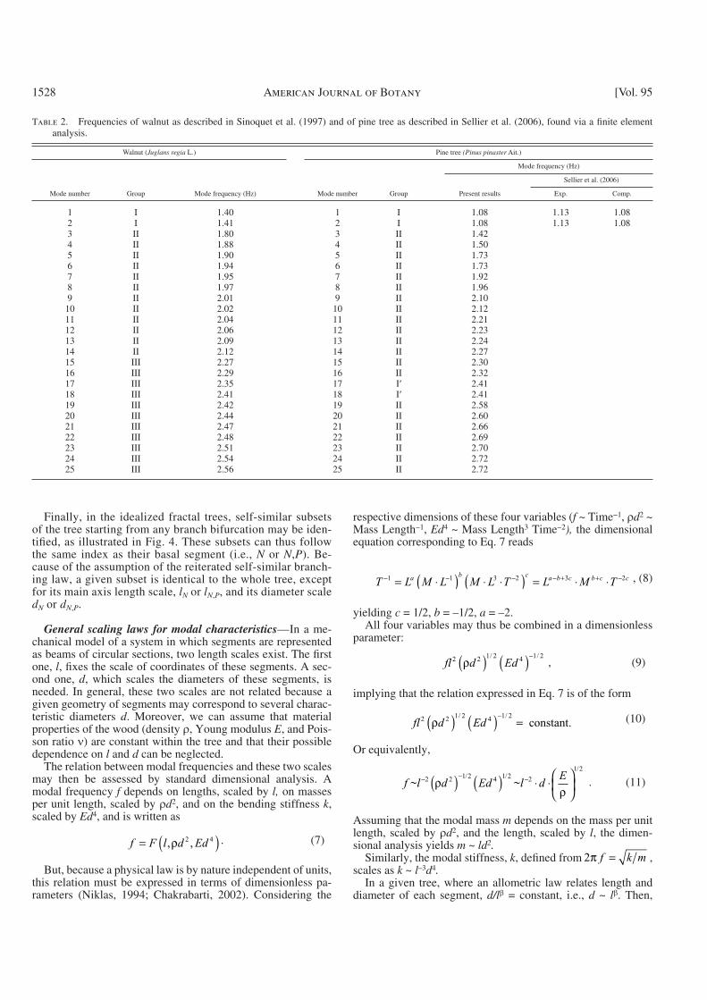
Table 2. Frequencies of walnut as described in Sinoquet et al. (1997) and of pine tree as described in Sellier et al. (2006) , found via a fi nite element analysis.

Walnut ( Juglans regia L . ) Pine tree (Pinus pinaster Ait.)

Mode number Group Mode frequency (Hz) Mode number Group

Mode frequency (Hz)

Present results

Sellier et al. (2006)

Exp. Comp.

1 I 1.40 1 I 1.08 1.13 1.082 I 1.41 2 I 1.08 1.13 1.083 II 1.80 3 II 1.424 II 1.88 4 II 1.505 II 1.90 5 II 1.736 II 1.94 6 II 1.737 II 1.95 7 II 1.928 II 1.97 8 II 1.969 II 2.01 9 II 2.10

10 II 2.02 10 II 2.1211 II 2.04 11 II 2.2112 II 2.06 12 II 2.2313 II 2.09 13 II 2.2414 II 2.12 14 II 2.2715 III 2.27 15 II 2.3016 III 2.29 16 II 2.3217 III 2.35 17 I 2.4118 III 2.41 18 I 2.4119 III 2.42 19 II 2.5820 III 2.44 20 II 2.6021 III 2.47 21 II 2.6622 III 2.48 22 II 2.6923 III 2.51 23 II 2.7024 III 2.54 24 II 2.7225 III 2.56 25 II 2.72


sidering only modes of symmetric deformations of subsets. As the general biometrical laws apply to subsets, the hypothesis to be tested is that the scaling laws derived from symmetric modes will capture the dimensional behavior of the whole group of modes involving the deformation of all the subsets of a given scale.

For a sympodial, idealized tree ( Fig. 5A ), the modal deforma-tions of three groups of symmetric modes (I, II, and III) can eas-ily be deduced from one to the other. Because of the symmetry of the branching pattern, a mode of group II is associated with the deformation of a subset with a fi xed part at its base. There-fore, the modal frequency of the group II of the whole tree can be considered as the frequency of a mode of group I of the subset if it is isolated. The dependence of fII on lII and dII should therefore be identical to the dependence of fI on lI and dI , hence yielding:

f

f

d l

d l

d

d

II

I

II II

I I

II

I

= =

−

−

−2

2

2ββ . (14)

Using the relation between successive diameters in a fractal sympodial tree, Eq. 3 yields

f

f

II

I

=−

λβ

β2

2 . (15)

Similarly, the frequency of modes in the group of order N is given by

f

f

N

I

N

=−( ) −( )

λβ

β

1 2

2 . (16)

Therefore, all frequencies can be deduced from the fi rst one, given the allometric parameter , and the area reduction param-eter at branching .

In the case of the model tree of monopodial type ( Fig. 5B ), the scale of a subset [N,P] depends on its central axis length and diameter, lN,P and dN,P . Introducing the relation between diam-eters and between lengths from Eq. 5 in Eq. 12, the correspond-ing frequency ratio can be defi ned as

f

f

N P N P,

I,I

= µ − −

−

λβ

β1 12

2 . (17)

from Eq. 11, the frequencies of modes are expected to depend on the scale of length and of diameter as follows:

f l d~ ~β

ββ−−

2

2 (12)

and similarly for the modal mass and stiffness:

m l d k l d~ ~ ~ ~1 2

1 2

4 3

4 3

++

−−

b

b

b b

b

b,. (13)

Relation between frequencies for a fractal tree— Due to the symmetries of the fractal structure, groups of modes can be de-duced and classifi ed according to their modal deformation ( Fig. 5 ). Some modes involve trunk deformation (group I in sympodial tree [ Fig. 5A ], group I,I in the monopodial tree [ Fig. 5B ]). Other modes involve mainly the bending deformation of the basal branch of all subsets of the same order (e.g., modes II for N = 2 subsets, modes III for N = 3 subsets in the sympodial tree [ Fig. 5A ], mode II,I for [2,1] subsets and II,II for [2,2] subsets in the monopodial tree [ Fig. 5B ]) with negligible deformation of up-stream segments. The deformation of upstream segments is strictly zero when the mode involves the symmetric deformation of two symmetric subsets as in Fig. 5 . In the modes where sym-metric subsets are deformed antisymmetrically, the lower part of the tree is slightly bent. But the elastic strain energy stored in this slight bending of the lower part of the tree is negligible compared to the energy stored in this same part due to modes with lower index. Consequently, scaling laws will be derived thereafter con-

Fig. 3. Examples of model fractal trees and parameters defi ning model trees. (A) Sympodial case, = 12.5 , and (B) monopodial case, = 30 ; (C) Branch slenderness coeffi cient, ; (D) branching ratios, and ; and (E) angle of branching connections, , illustrated here in the case of two lateral branches.

Fig. 4. Identifi cation of subsets in (A) the sympodial and (B) the mo-nopodial model trees. Subsets are circled in black or gray.


Numerical illustration of scaling laws on idealized frac-tal trees— The scaling laws derived in the preceding section were applied to two particular occurrences of the idealized trees, one sympodial and one monopodial. The allometric and geometrical parameters defi ning their geometry are given in Table 3 .

Modal frequencies— Instantiating the values of the allomet-ric and geometrical parameters in Eqs. 16 and 17 using Table 3 , the series of frequencies for the sympodial [ N ] and monopodial [N , P ] idealized trees read, respectively, as

f

f

N

N

I

=−

21

6 , f

f

N PN

P

,

I,I

=

−−

63

2

1

6

1

6 . (23)

These series of frequencies are illustrated in Fig. 6A and 6B . In the case of the sympodial [ N ] idealized tree in Fig. 6A , frequen-cies of group of modes are seen to increase progressively. Con-versely, for the monopodial [ N , P ] idealized tree in Fig. 6B , sets of frequencies corresponding to the double-indexed branching pattern can be observed. For a given value of N (i.e., for sequen-tial subtrees along a given monopodial axis, e.g., N = 2), fre-quencies increased progressively with P . For a given P (i.e., for series of lateral subtrees, e.g., P = 1), frequencies also increased with N . From Eq. 23, it appears that fN,P values from different groups intercalate, e.g., f2,5 < f3,1 < f2,6 . In the two cases, how-ever, the organization of frequencies is clearly dependent on the architecture, through the parameters and of area reduction at branching, and on the slenderness allometry, through the pa-rameter .

By the same token, the modal mass reads

m

m

NN

I

=− −( )

24

31

, m

m

N PN

P

,

I,I

=− −( )

− −( )6

3

2

4

31

4

31

. (24)

Localization of modal mass and modal stiffness— The lo-calization in height of the centers of bending energy and the centers of kinetic energy for the modes in each idealized tree were determined from Eqs. 21 and 22 using the values for pa-rameters from Table 3 , then plotted as a function of the corre-sponding modal frequency ( Fig. 6C, D ). In both trees, the distance between the center of bending energy and the center of kinetic energy is a decreasing function of the modal frequency. Modes thus tended to be more local as their modal frequency increased.

In the sympodial tree in Fig. 6C , modes localized higher in the tree as the modal frequency increased. In the monopodial tree in Fig. 6D , the mixed axial and lateral branching pattern

Through similar arguments, the modal mass of the groups of order N and [ N , P ] for a sympodial tree and a monopodial tree read, respectively, as

m

m

N

N

I

=−( ) +( )

λβ

β

1 1 2

2 , m

m

N P N P,

I,I

= µ − −

+

λβ

β1 11 2

2 . (18)

Center of bending energy and center of kinetic energy— Com-paring the spatial distributions of modal displacements Φ j along the tree is not straightforward. To summarize the localization of displacement associated with a given mode, one may defi ne two geometrical points: the center of kinetic energy of the mode and the center of elastic bending strain energy of the mode.

The modal center of kinetic energy is located at an elevation zK such that

z S d S z dK ⋅ ⋅ = ⋅ ⋅∫ ∫ρ ρΦ Φ Ω Φ Φ ΩΩ Ω

. (19)

Similarly, the modal center of bending strain energy, zB , is de-fi ned by a vertical position

z EI d EI z dB ⋅ ⋅ = ⋅ ⋅∫ ∫γ γ γ γΩ ΩΩ Ω

, (20)

where γ is the curvature associated with the modal displace-ment Φ and where integration is performed over the whole tree ( ).

These two parameters scale, respectively, as zK ~ l ~ d1/ and zB ~ l ~ d1/ . Exploiting again the assumption of reiterated trees, the position of the centers for a mode [ N , P ] reads

z z zN P N P

P N

, ,

/ cosK

I,I

K= + µ ( )−−( ) −

1

1 2 1 21β βλ α , (21)

z z zN P N P

P N

, ,

/ cosB

I,I

B= + µ ( )−−( ) −

1

1 2 1 21β βλ α , (22)

where zN,P is the elevation of the branching bifurcation (see Ap-pendix 1 for the geometrical derivation).

Fig. 5. (A) Modes of groups I, II, and III of the sympodial model tree. (B) Modes [I,I], [II,I] and [II,II] of the monopodial model tree. ( ) and ( ) represent the centers of bending energy and kinetic energy respectively.

Table 3. Slenderness coeffi cients , lateral and axial branching ratios and , respectively, and branching angles used to illustrate

the two idealized trees. A slenderness coeffi cient equal to 3/2 has frequently been used in the literature (see McMahon and Kronauer, 1976 ; Moulia and Fournier-Djimbi, 1997), and branching ratios were chosen to follow Da Vinci ’ s surface conservation law ( Prusinkiewicz and Lindenmayer, 1996 ).

Idealized tree

Sympodial 3/2 1/2 0 20 Monopodial 3/2 1/6 2/3 30


TEST OF THE SCALING LAWS ON MODELS OF REAL

TREES

The scaling laws for modal frequencies (Eqs. 16 and 17) and localization of the centers of kinetic and bending energy (Eqs. 21 and 22) were then applied to the two “ real ” tree models (i.e., the sympodial walnut and the monopodial pine, Fig. 1 ). The results were then compared with the modal characteristics com-puted using 3D fi nite element models (see section Modal analy-sis of a walnut and a pine tree ; Fig. 2 ).

resulted in the centers of bending energy and the centers of ki-netic energy being scattered all along the trunk. Modes related to group of subtrees localized at a constant number of lateral branching (fi xed N , changing P ) were found to be localized higher in the tree as the modal frequency increased. But the in-tercalation of modes both in terms of spatial localization and frequency is obvious. The modal analysis of idealized trees thus suggests that the localization of modes in the structure depends of the tree architecture via its branching pattern (sympodial vs. monopdial).

Fig. 6. Vibration modes of the sympodial and monopodial idealized trees. Modal frequencies, relative to the fi rst one, as a function of the index of the corresponding subsets in the case of the (A) sympodial and (C) monopodial trees, respectively. Vertical position of the centers of bending energy ( - ) and of the centers of kinetic energy ( - ) as a function of the frequency, respectively in the (C) sympodial and (D) monopodial trees.


defi ned in the section Modal analysis of a walnut and a pine tree ( Fig. 8 ).

Case of the walnut — Figure 8A displays the frequencies of the three groups of modes (I, II, and III, see Fig. 2A, C and section Modal analysis of a walnut and a pine tree ) estimated using the 3D FEM vs. the group number N . On the same graph, the dotted lines show the frequencies predicted using Eq. 16 with the 90% confi dence range of parameters as in Table 4 . The same comparison is held for the values for the height of the bending and kinetic energy centers (using Eqs. 21 and 22), in Fig. 8B and C . Though the geometry of the real walnut is much more complex than that of the idealized frac-tal sympodial tree, the prediction using the scaling laws quite closely brackets the range of modal characteristics of the FEM model. The positions of the centers of bending and ki-netic energy are particularly well estimated, with the excep-tion of two points.

Case of the pine — As emphasized previously, the case of the monopodial tree is much more complex, due to the dou-ble index dependence related to the two kinds of branching, axial and lateral. We will focus on the characteristics of the modes labeled II in the section Modal analysis of a walnut and a pine tree (see Fig. 2B, D ), corresponding to the motion of lateral subsets. In terms of the double index reference, these are modes involving [2, P ] subsets. The scatter of modal characteristics is higher in the pine tree than in the walnut tree ( Fig. 8D – F ). The scaling law derived from idealized fractal monopodial tree still brackets from 60 to 75% of the outputs of the FEM model. But half of the confi dence inter-vals from the scaling laws does not contain any output of the FEM model.

Moreover, modes of group I cannot be predicted, using the scaling laws applied to subsets of the tree because the corre-sponding deformation cannot be defi ned as the deformation of a subset. For instance, the frequencies of I are in the order of 2.4 Hz for the pine tree, while those corresponding to subset [1,2] are about 1.16 Hz.

DISCUSSION

An approach of the complex oscillatory behavior of trees through modal and scaling analyses — Despite its standard use in mechanical engineering ( Gerardin and Rixen, 1994 ), modal analysis has only been used in a few studies to analyze the dy-namic characteristics of trees in relation to their 3D architecture ( Fournier et al., 1993 ; Moore and Maguire, 2005 ; Sellier et al., 2006 ). Compared to the analysis of the vibrational behavior of separated elements of the tree such as trunk, branches (e.g., Mc-Mahon and Kronauer, 1976 ; Spatz et al, 2007 ), modal analysis takes into account the additional fact that as a whole, the tree is a mechanical structure. As a consequence, elastic strain energy is almost instantaneously distributed over the whole tree struc-ture, and vibrations involving the whole tree can occur. Such vibrations can involve several parts of the tree together and can thus be more complex than that of isolated parts. Indeed, models connecting a large number of small damped oscillators con-nected together — each oscillator modeling a branch subsys-tem — have been proposed recently ( James et al., 2006 ). However, such models are not parsimonious, and their behavior may be diffi cult to analyze quantitatively. Under the classical assumption

Determination of biometrical parameters for the scaling law— Orthogonal regressions (SAS version 9.1, procedure In-sight Fit) were applied to estimate slenderness allometric coef-fi cients, , and branching ratios, and , from the MTG tree databases of the walnut and pine geometries. Slenderness coef-fi cients, , were estimated from the linear orthogonal regression log(d ) = log( l ) + k ( Niklas, 1994 ). Lateral branching ratios, , were estimated from linear orthogonal regression ( dN ) 2 = (d N-

1 ) 2 and axial branching ratio, (in monopodial tree), from ( d1,P ) 2

= ( d1,P-1 ) 2 . Regression coeffi cients, root mean square errors,

coeffi cients of determination, and 90% confi dence intervals (Dagnelie, 2006) are reported in Table 4 .

Case of the walnut tree— Parameters were estimated using data from the fi rst three order branches with diameters and lengths larger than 1 cm and 1 m, respectively ( Fig. 7A, B ). A highly signifi cant, tight allometric relation was found between land d ( Fig. 7A ), capturing 87% of the total variance, with only two outlying points corresponding to the trunk and to a cut branch. The relation between dN+1 and dN was a little bit more biased, but still a highly signifi cant could be defi ned. The sympodial branching pattern of the walnut implies an axial branching ratio equal to 0. The angle of branching has been found to vary between 0 and 40 , a mean angle of branching,

= 20 , was retained.

Case of the pine tree— Parameters were estimated using data from the fi rst two order branches ( Fig. 7C – E ). The slenderness

( Fig. 7C ) and the longitudinal area reduction ( Fig. 7E ) were statistically signifi cant. The axial branching ratio ( Fig. 7D ) was also signifi cantly different from zero, but the relation be-tween the cross-sectional area of the parent segment and of lat-eral branches was very poor [the slope of the regression model with the intercept is not signifi cantly different from zero with probability p ( > F ) = 0.13] . The mean angle of branching was

= 30 .

Application of scaling laws— Using the parameters corre-sponding to the two real trees ( Table 4) , we applied the scaling laws derived in the Theoretical considerations section to the case of each real tree, then compared the results to the modal characteristics computed using the 3D fi nite element models

Table 4. Slenderness coeffi cients , lateral and axial branching ratios and , respectively, and branching angles estimated from walnut and pine tree geometries (orthogonal regression coeffi cients, confi dence intervals at 90% level [CI), coeffi cients of determination [ R2 ], and root mean square of the residual errors [ res ]). Tree geometries are from Sinoquet et al. (1997) and Sellier and Fourcaud (2005) , respectively. Note that for and , the regressions were obtained with no intercept so that the R2 value cannot be compared directly with that related to a standard linear regression, and signifi cance levels are to be related to a null hypothesis where the dependant variable is equal to zero (for a more detailed discussion, see Freund and Littel, 1991 ).

Tree

Walnut 1.37 0.25 0 20 CI 1.25 < < 1.49 0.22 < < 0.29 R2 0.87 0.74 res 0.2 0.008Pine 1.38 0.038 0.74 30 CI 1.25 < < 1.52 0.032 < < 0.044 0.71 < < 0.79 R2 0.85 0.59 0.97 res 0.086 11.92 5.33


its strict defi nition, modal analysis only deals with small displace-ments, as is the case for trees submitted to moderate winds. But with large winds, large displacements occur, and geometric non-linearities such as strong streamlining or branch collisions have to be taken into account ( de Langre, 2008 ). Such nonlinear be-haviors are still a very active area of research in the mechanics of fl uid – structure interactions ( de Langre and Axisa, 2004 ). How-ever, some numerical methods for predicting fl ow-induced vibra-tions in nonlinear cases still involve modal analysis ( Axisa et al., 1988 ), meaning that modal analysis is still a robust starting point for the analysis of the dynamic excitability under strong winds.

Branches are important to the tree dynamics — The detailed FEM modal analysis of entirely digitized trees with a very large contrast in their mechanical architecture and modal behavior confi rmed and extended previous reports: modes involving sig-nifi cant branch deformation could have frequencies very close to — and even rank in between — modes deforming mainly the trunk ( Fournier et al., 1993 ; Moore and Maguire, 2005 ; Sellier and Fourcaud, 2005 ; James et al., 2006 ; Sellier et al., 2006 ). As many as 25 modes could be found with frequencies between one and two times the most basal mode involving the trunk and

of relatively small displacements, this complex behavior can be analyzed as the superposition of a (large) set of much simpler free-vibration modes with characteristic modal frequency and modal deformation and modal inertial mass. These modes are mechanical attributes of the whole tree structure, its intrinsic dy-namical characteristics independent of any particular load. They characterize the vibrational excitability of a given tree. A given load, say, a turbulent wind with specifi c frequencies and spatial distributions, will excite only the modes with compatible fre-quencies and modal shapes. Becausee universal wind spectra have been obtained showing that mechanically active wind loads in trees typically occur in the 0 – 10 Hz band ( Stull, 1988 ), and the drag mainly applies to the leaf-bearing terminal segments, it is possible to focus on the subset of modes in this frequency band and with modal deformations involving signifi cant dis-placements of the branch tips, as done in this study.

Because they are based on very detailed and extensive archi-tectural and mechanical data, modal analyses can also provide guidelines for defi ning simpler models, as illustrated through scaling analysis (and discussed later).

Before discussing the major insights on tree mechanics ob-tained through this method, we should discuss its limitations. In

Fig. 7. Biometrical relations in the walnut and the pine trees. (A, C) Allometric relations between length and diameter of branches in (A) the walnut and (C) the pine tree. ( — ) Orthogonal regression D ~ L , with = 1.37 (A) and = 1.38 (C). (B, D) Branches cross-sectional areas before and after a lateral branching in (B) the walnut and (D) the pine tree. ( — ) Orthogonal regression ( dN ) 2 = ( dN-1 )

2 , with (B) = 0.25 and (D) = 0.038. (E) Cross-sectional areas of the trunk before and after a branching in the case of the monopodial pine tree. ( — ) Orthogonal regression ( d1,P ) 2 = ( d1,P-1 )

2 , = 0.74. Gray areas in the graphs correspond to the 90% confi dence level (see Table 4 ). ( ) measured data from Sinoquet et al. (1997) and Sellier and Fourcaud (2005) .


Scaling laws can be defi ned — As hypothesized, and despite the aforementioned complexity of the 3D architecture and modal structure of real trees, scaling laws based on the assump-tions of (1) idealized allometric fractal trees and (2) symmetric modes of branches, are able to explain a large part of the spatial and temporal characteristics of the modes involving the succes-sive orders of branches relative to the fi rst mode deforming the trunk ( Fig. 8 ). The distribution of modal characteristics was particularly well predicted in the case of the tree with highest modal density and where the branch modes are the most salient, i.e., the sympodial walnut tree. Moreover, in both trees, scaling laws were able to predict correctly the relative ranking of the different types of modes ( Fig. 8A ), validating the hypothesis that the dimensional analysis of the symmetric modes of ideal-ized fractal trees can capture a large part of the scaling of modal settings in real trees (frequencies and localization of bending and kinetic energy), although more advanced analysis may be conducted for monopodial trees.

Such scaling law has two major uses. From a methodological and practical point of view, the overall dynamics of a complex tree can be reduced to (1) the measurement or estimation of the most basal mode, which is the easiest to characterize and has been studied or modeled in numerous studies (e.g., Gardiner, 1992 ; Spatz and Zebrowski, 2001 ); (2) a standard description of the branching mode, i.e., sympodial vs monopodial mode

with a typical modal spacing as low as 0.1 Hz, consistent with the results of James et al. (2006) and Spatz et al. (2007) .

Although these modes are complex, they can be classifi ed using their frequencies and modal deformation. In this study, no modes involving an infl ection in their modal deformation, I (i.e., second modes of the trunk, I in our labeling), could be observed within the 25 fi rst modes in the walnut tree, whereas for the pine tree, I only rank 17th and 18th (i.e., 14 modes II involving fi rst order branches ranked in between the fundamen-tal mode of the trunk I and its I mode). This is quite in contrast with claims from the literature, mostly about adult conifer trees, on which only fi rst I and second I bending modes of the trunk have been reported (e.g., White et al., 1976 ; Mayer, 1987 ; Has-sinen et al., 1998 ; Kerzenmacher and Gardiner, 1998 ). How-ever, in these studies only the strains in the trunk were measured or modeled; therefore, only modes involving signifi cant defor-mation of the trunk could be recorded. Indeed, when analyzing the vibration modes of an adult maritime pine ( Pinus pinaster ) using fi nite element analysis, Fournier et al. (1993) also found that modes concentrated in frequency and that modes of the second group ranked between the fi rst and the second bending modes of the trunk. Branch deformation is thus an important aspect of trees dynamics whatever the architectures and size (see also Fournier et al., 1993 ; Sellier and Fourcaud, 2005 ; Moore and Maguire, 2005 ; Spatz et al., 2007 ).

Fig. 8. Comparison of the prediction from the scaling laws with the fi nite element results on the true tree geometry: (A) frequencies, (B) centers of kinetic energy ( ), (C) centers of bending energy ( ) of modes of the walnut tree, and (D) frequencies, (E) centers of kinetic energy ( ), (F) centers of bending energy ( ) of modes [2, P ] of the pine tree. ( and ) are results from the FEM on true tree geometries; gray areas are predictions from the scaling laws, Eqs. 12, 13, 18, and 19, using idealized tree models.


trees during their architectural development. This specifi c bio-mechanical design of the trees requires a consistent tuning of both (1) branching symmetries within the architecture and (2) the secondary growth balance between parent and axillary branches (as reported by Watt et al., 2005. Moreover, this con-sistent tuning should be effi cient in highly different architec-tural patterns (monopods vs. sympods) and is thus very likely to have resulted from adaptation.

These structural compartmentalization and scaling similari-ties are probably important in making the overall biological control over the multimodal dynamics of the tree more tracta-ble, whatever its size. Assessing how this gain in control may be benefi cial for species adaptation and individual acclimation to wind should be the matter of specifi c future investigations. Indeed, scaling laws give only approximations, and clear differ-ences were found in the modal spatial patterning between mo-nopodial and sympodial trees. Moreover, trees in a forest stand may have more signifi cant shoot abrasion or crown asymmetry. At last, competition for resources and photomorphogenetic re-sponses to shade may interact with the mechanoperceptive ac-climation to wind ( Fournier et al., 2005 ). But some elements affecting the biomechanical signifi cance of multimodal scaling of trees to the response to wind load can already be directly discussed from our results.

Signifi cance of multimodal dynamics and scaling laws to the responses of trees to wind— Wind excites trees through the drag force applied to the constitutive elements of the trees, branches, and possibly leaves or needles. From surface area considerations, most of the drag thus occurs at in the distal, pos-sibly leafy, segments of the tree. All the modes in this study have a common characteristic: their larger displacements sits on the extremities of the tree. Therefore, they should recipro-cally all be excited by a force applied at the extremities, such as the wind-drag force ( Gerardin and Rixen, 1994 ). Moreover, be-cause wind spectra usually have a large frequency band ( Rau-pach et al., 1996 ) overlying most of the modal frequencies of the considered modes, several modes may be excited directly by highly fl uctuating winds. As a consequence, the two types of tree architectures studied here should have a dense multimodal response to gusts involving a very signifi cant contribution of branches of all the orders.

James et al. (2006) and Spatz et al. (2007) have argued that dynamics including branch deformation with close modal fre-quencies could be benefi cial to the tree by enhancing aerody-namic dissipation through a mechanism called multiple resonance damping or multiple mass damping. A prerequisite for this mechanism to occur is a multimodal behavior of the tree, with high modal density in the frequency range and signifi -cant branch deformations, exactly what was found here for trees with contrasting architectures. This dense multimodal dynam-ics, a consequence of the branched structure, can then be inter-preted as a strategy to prevent the trunk from bending excessively until the rupture. It should be noted, however, that the high modal density observed in our two trees did not reach the al-most perfect tuning in the modal frequencies of branches larger than 0.5 m reported by Spatz et al. (2007) for a (monopodial) Pseudostuga menziesii tree. A similar result in our study would have meant either and = 1 or = 2, which can be rejected statistically in our two trees ( Table 4 ). However in our study, possible variations in the longitudinal Young ’ s modulus along the branch (that have been reported by Spatz) were not considered. It would be interesting to further investigate if the distribution

( Barthelemy and Caraglio, 2007 ); and (3) three simple biomet-rical parameters that have been measured in many biomechani-cal and ecological studies (e.g., McMahon and Kronauer, 1976 ). This compact description of the overall dynamics of a complex tree is to be compared with the extensive work on detailed 3D digitizing ( Sinoquet and Rivet, 1997 ) followed by complete modal analysis. It would be interesting though to test these scal-ing laws in trees of other species and other sizes, so that the accuracy in the prevision through these simplifi ed laws could be assessed more completely.

From a more fundamental perspective, these scaling laws give direct insights into the signifi cance of tree architecture and geometry for its modal behavior and thus to its excitability to wind and its possible mechanoperceptive control, as discussed next.

Effects of architecture and biometrical characteristics on modal content: Tuning and compartmentalization— Both area reduction ratios and the slenderness coeffi cient affect the rela-tive frequency and the location of modes (see Eqs. 16 and 21), whereas the branching angle only affects the spatial localiza-tion of the modes. In all the cases, the effects of the parameters are nonlinear and mixed.

For example, in the case of the sympodial tree, variations in and both infl uence the value of the frequency of a given

group of modes. In the natural ranges estimated from our data ( Table 4 ), a decreasing (i.e., a higher reduction in the cross-sectional area at branching) increases the relative frequency of a given group of mode. A decreasing (i.e., a tree with higher slenderness) also increases the relative frequency of a given group of mode. It should be noted here that both and have been reported to be under similar control of wind mechano-perception through thigmomorphogenetic secondary growth responses ( Telewski, 2006 ; Watt et al., 2005 ). Thus, thigmo-morphogenetic responses may be able to tune the multimodal frequencies range of the whole tree, whatever the genetic spe-cifi c traits of its architecture. It is, moreover, striking that two trees as geometrically different as an old walnut tree and a young pine tree could present fundamental modes in the range of 1 – 1.5 Hz with a large number of their branch modes in the 2.5 – 3 Hz band, consistent with many reports in the literature (B. Roman, Ecole Superieure de Physique et Chimie Industri-elles de Paris (ESPCI), personal communication). This similar-ity in modal frequencies may point toward some modal tuning controlling the biometrical parameters of the trees (and thus of the scaling laws). The effectiveness of this acclimation process remains to be studied, but the current study provides useful tools to do so.

Last but not least, a very unexpected salient conclusion that is captured by the scaling laws is that branching and secondary growth are tuned so that the reduction of cross sectional area at branching points ( and eventually in monopods), induce a clear structural compartmentalization of the modal spatial dis-tribution and a scaling similarity between successive modes. Whatever the architecture, modes have been found to be more and more local as their modal frequency increases. And both their modal frequencies and modal mass are scaled recursively to that of the fi rst mode of the whole tree. These compartmen-talization and scaling similarity are not mechanical necessities. As previously stated, the elastic strain energy underlying modal behavior is distributed almost instantaneously over the whole structure; so that structural compartmentalization and scaling similarities result from a specifi c biomechanical design of the


Gardiner, B. A., and C. P. Quine . 2000 . Management of forests to re-duce the risk of abiotic damage – A review with particular reference to the effects of strong winds. Forest Ecology and Management 135 : 261 – 277 .

Gerardin, M., and D. Rixen . 1994 . Mechanical vibrations: Theory and application to structural dynamics. Wiley, Chichester, UK.

Gillison, A. N. 1994 . Woodlands. In R. H. Groves [ed.], Australian veg-etation, 2nd ed., 227 – 255. Cambridge University Press, Cambridge, UK.

Godin, C., E. Costes, and H. Sinoquet . 1999 . A method for describing plant architecture which integrates topology and geometry. Annals of

Botany 84 : 343 – 357 . Hassinen, A., M. Lemettinen, H. Peltola, S. Kellomaki, and B.

Gardiner . 1998 . A prism-based system for monitoring the swaying of trees under wind loading. Agricultural and Forest Meteorology 90 : 187 – 194 .

James, K. R., N. Haritos, and P. K. Ades . 2006 . Mechanical stability of trees under dynamic loads. American Journal of Botany 93 : 1522 – 1530 .

Kerzenmacher, T., and B. A. Gardiner . 1998 . A mathematical model to describe the dynamic response of a spruce tree to the wind. Trees —

Structure and Function 12 : 385 – 394 . Mayer, H. 1987 . Wind-induced tree sways. Trees — Structure and

Function 1 : 195 – 206 . McMahon, T. A., and R. E. Kronauer . 1976 . Tree structures: Deducing

the principle of mechanical design. Journal of Theoretical Biology

59 : 443 – 466 . Meinzer, F. C., M. J. Clearwater, and G. Goldstein . 2001 . Water trans-

port in trees: Current perspectives, new insights and some controver-sies. Environmental and Experimental Botany 45 : 239 – 262 .

Moore, J. R., and D. A. Maguire . 2005 . Natural sway frequencies and damping ratios of trees: Infl uence of crown structure. Trees — Structure

and Function 19 : 363 – 373 . Moore, J. R., and D. A. Maguire . 2008 . Simulating the dynamic behavior

of Douglas-fi r trees under applied loads by the fi nite element method. Tree Physiology 28 : 75 – 83 .

Moulia, B., C. Coutand, and C. Lenne . 2006 . Posture control and skeletal mechanical acclimation in terrestrial plants: implications for mechani-cal modeling of plant architecture. American Journal of Botany 93 : 1477 – 1489 .

Moulia, B., and M. Fournier-Djimbi . 1997 . Optimal mechanical design of plant stems: The models behind the allometric power laws. In G. Jeronimidis and J. F. V. Vincent [eds.], Plant biomechanics, 43 – 55. Centre for Biomimetics, University of Reading, Reading, UK.

Niklas, K. J. 1992 . Plant biomechanics: An engineering approach to plant form and function. University of Chicago Press, Chicago, Illinois, USA.

Niklas, K. J. 1994 . Plant allometry: The scaling of form and process. University of Chicago Press, Chicago, Illinois, USA.

Prusinkiewicz, P., and A. Lindenmayer . 1996 . The algorithmic beauty of plants, 2nd ed. Springer-Verlag, New York, New York, USA.

Raupach, M. R., J. J. Finnigan, and Y. Brunet . 1996 . Coherent ed-dies and turbulence in vegetation canopies: The mixing-layer analogy. Boundary-Layer Meteorology 78 : 351 – 382 .

Sellier, D., and T. Fourcaud . 2005 . A mechanical analysis of the relation-ship between free oscillations of Pinus pinaster Ait. saplings and their aerial architecture. Journal of Experimental Botany 56 : 1563 – 1573 .

Sellier, D., T. Fourcaud, and P. Lac . 2006 . A fi nite element model for investigating effects of aerial architecture on tree oscillations. Tree

Physiology 26 : 799 – 806 . Shigo, A. 1986 . A new tree biology. Shigo and Trees, Associates,

Durham, New Hampshire, USA. Sinoquet, H., and P. Rivet . 1997 . Measurement and visualization of the

architecture of an adult tree based on a three-dimensional digitising device. Trees — Structure and Function 10 : 265 – 270 .

Sinoquet, H., P. Rivet, and C. Godin . 1997 . Assessment of the three-dimensional architecture of walnut trees using digitising. Silva

Fennica 31 : 265 – 273 . Spatz, H.-C., F. Br ü chert, and J. Pfisterer . 2007 . Multiple resonance

damping or how do trees escape dangerously large oscillations? American Journal of Botany 94 : 1603 – 1611 .

of wood stiffness along branches could be controlled to further enhance the modal density.

Modes can also be characterized in terms of the localization of their bending centers, i.e., the zone of signifi cant bending of the tree. The fi rst bending modes result in deformation on the trunk, while higher frequency modes result in deformations lo-calized in higher orders of branching in the tree, with a different spatial pattern in monopodial and sympodial trees. This com-partmentalization may have consequences for windbreaks. In-deed, some studies have reported branch breaks occurring before trunk or roots breaks, with obvious benefi t for wind re-sistance ( Cullen, 2002 ; Watt et al., 2005 ). Such mechanical modal compartmentalization of the wind hazards would then present analogies with compartmentalization strategies in front of hydric stresses ( Meinzer et al., 2001 ) and perhaps pathogens ( Shigo, 1986 ). But this mechanical modal compartmentaliza-tion of the wind hazards remains to be confi rmed experimen-tally over a larger range of situations and species.

LITERATURE CITED

Axisa, F., J. Antunes, and B. Villard . 1988 . Overview of numerical methods for predicting fl ow-induced vibrations. Journal of Pressure

Vessel Technology 110 : 6 – 14 . Barthelemy, D., and Y. Caraglio . 2007 . Plant architecture: A dynamic,

multilevel and comprehensive approach to plant form, structure and ontogeny. Annals of Botany 99 : 375 – 407 .

Br ü chert, F., and B. A. Gardiner . 2006 . The effect of wind ex-posure on the tree aerial architecture and biomechanics of Sitka spruce ( Picea sitchensis , Pinaceae). American Journal of Botany

93 : 1512 – 1521 . Chakrabarti, S. 2002 . The theory and practice of hydrodynamics and

vibration. World Scientifi c, Singapore, Singapore. Coutand, C., and B. Moulia . 2000 . A biomechanical study of the effect

of a controlled bending on tomato stem elongation. II. local mechani-cal analysis and spatial integration of the mechanosensing. Journal of

Experimental Botany 51 : 1825 – 1842 . Cullen , S. 2002 . Tree and wind: Wind scales and speeds. Journal of

Arboriculture 28: 237 – 242. Dagnelie, P. 2006 . Statistique th é orique et appliqu é e. Tome 2. Inf é rence

statistique à une et à deux dimensions. De Boeck et Larcier, Brussells, Belgium.

De Langre, E. 2008 . Effects of wind on plants. Annual Review of Fluid

Mechanics 40 : 141 – 168 . De Langre, E., and F. Axisa [eds.]. 2004. Proceedings of the 8th

International Conference on Flow-Induced Vibration, Paris, France, 2004 . Ecole Polytechnique, Paris, France.

Fournier, M., P. Rogier, E. Costes, and M. Jaeger . 1993 . Mod é lisation m é canique des vibrations propres d ’ un arbre soumis aux vents, en fonction de sa morphologie. Annales des Sciences Forestieres 50 : 401 – 412 .

Fournier, M., A. Stokes, C. Coutand, T. Fourcaud, and B. Moulia . 2005 . Tree biomechanics and growth strategies in the context of for-est functional ecology. In A. Herrel, T. Speck, and N. Rowe [eds.], Ecology and biomechanics: A biomechanical approach of the ecol-ogy of animals and plants, 1 – 33. CRC Taylor & Francis, Boca Raton, Florida, USA.

Freund, R. J., and R. C. Littel . 1991 . SAS, System for regression, 2nd ed. SAS series in statistical applications. SAS Institute, Cary, North Carolina, USA.

Gardiner, B., H. Peltola, and S. Kellomaki . 2000 . Comparison of two models for predicting the critical wind speeds required to damage co-niferous trees. Ecological Modelling 129 : 1 – 23 .

Gardiner, B. A. 1992 . Mathematical modelling of the static and dynamic characteristics of plantation trees. In J. Franke and A. Roeder [eds.], Mathematical modelling of forest ecosystems, 40 – 61. Sauerl ä nder, Frankfurt/Main, Germany.


Spatz, H.-C., and J. Zebrowski . 2001 . Oscillation frequencies of plant stems with apical loads. Planta 214 : 215 – 219 .

Stull, R. B. 1988 . An introduction to boundary layer meteorology. Kluwer, Dordrecht, Netherlands.

Telewski, F. W. 2006 . An unifi ed hypothesis of mechanoperception in plants. American Journal of Botany 93 : 1466 – 1476 .

Verpeaux, P., T. Charras, and A. Millard . 1988 . CASTEM 2000, une approche moderne du calcul des structures. In J. M. Fouet, P.

Ladev è ze, and R. Ohayon [eds.], Calcul des structures et intelligence artifi cielle, 261 – 271, Pluralis, Paris, France.

Watt, M. S., J. R. Moore, and B. McKinlay . 2005 . The infl uence of wind on branch characteristics of Pinus radiata. Trees (Berlin)

19 : 58 – 65 . White, R. G., M. F. White, and G. J. Mayhead . 1976 . Measurement of the

motion of trees in two dimensions. Technical Report 86. Institute of Sound and Vibration Research, University of Southampton, Southampton, UK.

Appendix 1.

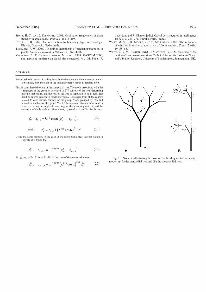
Because the derivation of scaling laws for the bending and kinetic energy centers are similar, only the case of the bending energy center is detailed here.

First is considered the case of the sympodial tree. The mode associated with the subgroups of the group N is related to 2 N-1 subsets of the tree, deforming like the fi rst mode, and the rest of the tree is supposed to be at rest. The bending energy center of a mode of group N is assessed from all the centers related to each subset. Subsets of the group N are grouped by two and related to a subset of the group N – 1. The relation between these centers is derived using the angle of branching, , the branching ratio, , and the elevation of the branching bifurcations, zN , see sketch on Fig. 9A . It reads

z z z zN N N N

B B− = −( )− − −1

1 2

1 2λ αβ cos , (24)

so that z z zN N

NB B= + ( )−

−

1

1 21

1λ αβ cos . (25)

Using the same process, in the case of the monopodial tree, see the sketch in Fig. 9B , it is found that

z z z zN P N P

P

N N, , , ,

B B− = µ −( )−−( )

−1

1 2

1 1 1

β , (26)

this gives, as Eq. 21 is still valid in the case of the monopodial tree

z z zN P N P

P N

, , ,cosB B= + µ ( )−−( ) −

1

1 2 1 21

1 1

β βλ α . (27)

Fig. 9. Sketches illustrating the positions of bending centers of several modes in (A) the sympodial tree and (B) the monopodial tree.

Documents

Mathieu Rodriguez, Emmanuel de Langre, and Bruno Moulia