Embed Size (px)
Citation preview

Mathematics of Machine LearningRajen D. Shah [email protected]
1 Introduction
Consider a pair of random variables (X, Y ) ∈ X × Y with joint distribution P0, where Xis to be thought of as an input or vector of predictors, and Y as an output or response.For instance X may represent a collection of disease risk factors (e.g. BMI, age, geneticindicators etc.) for a subject randomly selected from a population and Y may representtheir disease status; or X could represent the number or bedrooms and other facilities ina randomly selected house, and Y could be its price. In the former case we may takeY = {−1, 1}, and this setting, known as the (two-class) classification setting, will be ofprimary interest to us in this course. The latter case where Y ∈ R is an instance of aregression setting. We will take X = Rp unless otherwise specified.
It is of interest to predict the random Y from X; we may attempt to do this via a(measurable) function h : X → Y , known as a hypothesis. To measure the quality of sucha prediction we will introduce a loss function
` : Y × Y → R.
In the classification setting we typically take ` to be the misclassification error
`(h(x), y) =
{0 if h(x) = y,
1 otherwise.
In this context h is also referred to as a classifier. In regression settings the squared error`(h(x), y) = (h(x)− y)2 is common. We will aim to pick a hypothesis h such that the risk
R(h) :=
∫(x,y)∈X×Y
`(h(x), y) dP0(x, y)
is small. For a deterministic h, R(h) = E`(h(X), Y ). In what follows we will take ` and Rto be the misclassification loss and risk respectively, unless otherwise stated.
A classifier h0 that minimises the misclassification risk is known as a Bayes classifier,and its risk is called the Bayes risk. Define the regression function η by
η(x) := P(Y = 1 |X = x).
Proposition 1. A Bayes classifier h0 is given by1
h0(x) =
{1 if η(x) > 1/2
−1 otherwise.1When η(x) = 1/2, we can equally well take h0(x) = ±1 and achieve the same misclassification error.
1

In most settings of interest, the joint distribution P0 of (X, Y ), which determines the op-timal h, will be unknown. Instead we will suppose we have i.i.d. copies (X1, Y1), . . . , (Xn, Yn)of the pair (X, Y ), known as training data. Our task is to use this data to construct aclassifier h such that R(h) is small.Important point: R(h) is a random variable depending on the random training data:
R(h) = E(`(h(X), Y ) |X1, Y1, . . . , Xn, Yn).
A (classical) statistics approach to classification may attempt to model P0 up to someunknown parameters, estimate these parameters (e.g. by maximum likelihood), and therebyobtain an estimate of the regression function (or the conditional expectation in the caseof least squares—see below). We will take a different approach and assume that we aregiven a class H of hypotheses from which to pick our h. Possible choices of H include forinstance
� H = {h : h(x) = sgn(µ+ xTβ) where µ ∈ R, β ∈ Rp};
� H ={h : h(x) = sgn
(µ+
∑dj=1 ϕj(x)βj
)where µ ∈ R, β ∈ Rd
}for a given dictio-
nary of functions ϕ1, . . . , ϕd : X → R.
� H ={h : h(x) = sgn
(∑dj=1wjϕj(x)
)where w ∈ Rd, ϕj ∈ B
}for a given class B of
functions f : X → R.
Technical note: In this course we will take sgn(0) = −1. (It does not matter muchwhether we take sgn(0) = ±1, but we need to specify a choice in order that the h definedabove are classifiers.)
Non-examinable material is enclosed in *stars*.
1.1 Brief review of conditional expectation
For many of the mathematical arguments in this course we will need to manipulate condi-tional expectations.
Recall that if Z ∈ R and W ∈ Rd are random variables with joint probability densityfunction (pdf) fZ,W then the conditional pdf fZ|W of Z given W satisfies
fZ|W (z|w) =
{fZ,W (z, w)/fW (w) if fW (w) 6= 0
0 otherwise,
where fW is the marginal pdf of W . When one or more of Z and W are discrete wetypically work with probability mass functions.
Suppose E|Z| < ∞. Then the conditional expectation function E(Z |W = w) is givenby
g(w) := E(Z |W = w) =
∫zfZ|W (z|w)dz. (1.1)
2

We write E(Z |W ) for the random variable g(W ) (note this is a function of W , not Z).This is not a fully general definition of conditional expectation (for that see the Stochas-
tic Financial Models course) and we will not use it. We will however make frequent use ofthe following properties of conditional expectation.
(i) Role of independence: If Z and W are independent, then E(Z |W ) = EZ. (Recall:Z and W being independent means P(Z ∈ A,W ∈ B) = P(Z ∈ A)P(W ∈ B) for allmeasurable A ⊆ R, B ⊆ Rd)
(ii) Tower property: Let f : Rd → Rm be a (measurable) function. Then
E{E(Z |W ) | f(W )} = E{Z | f(W )}.
In particular, E{E(Z |W ) |W1, . . . ,Wm} = E(Z|W1, . . . ,Wm) for m ≤ d. Takingf ≡ c ∈ R and using (i) gives us that E{E(Z |W )} = E(Z) (as f(W ) is a constant itis independent of any random variable).
(iii) Taking out what is known: If EZ2 <∞ and f : Rd → R is such that E[{f(W )}2] <∞ then E{f(W )Z |W} = f(W )E(Z |W ).
(iv) Best least squares predictor: With the conditions in (iii) above, we have
E(Z − f(W ))2 = E{Z − E(Z |W )}2 + E{E(Z |W )− f(W )}2. (1.2)
Indeed, using the tower property,
E(Z − f(W ))2 = E(Z − E(Z |W ) + E(Z |W )− f(W ))2
= E{Z − E(Z |W )}2 + E{E(Z |W )− f(W )}2
+ 2EE[{Z − E(Z |W )}{E(Z |W )− f(W )} |W ],
but by ‘taking out what is known’, half the final term is
E[{E(Z |W )− f(W )}E{Z − E(Z |W ) |W}︸ ︷︷ ︸=0
] = 0.
Property (iv) shows that the h : X → R minimising R(h) under squared loss is h0(x) =E(Y |X = x).
Probabilistic results can be ‘applied conditionally’, for example:
Conditional Jensen. Recall that f : R→ R is a convex function if
tf(x) + (1− t)f(y) ≥ f(tx+ (1− t)y
)for all x, y ∈ R and t ∈ (0, 1).
The conditional version of Jensen’s inequality states that if f : R → R is convex andrandom variable Z has E|f(Z)| <∞, then
E(f(Z) |W
)≥ f
(E(Z |W )
).
3

1.2 Bayes risk
Proof of Proposition 1. We have R(h) = P(Y 6= h(X)) = EP(Y 6= h(X) |X), so h0(x)must minimise over h(x)
P(Y 6= h(X) |X = x) = P(Y = 1, h(x) = −1 |X = x) + P(Y = −1, h(x) = 1 |X = x)
= P(Y = 1 |X = x)1{h(x)=−1} + P(Y = −1 |X = x)1{h(x)=1}
= 1{h(x)=−1}η(x) + 1{h(x)=1}(1− η(x)).
When η(x) > 1 − η(x) and so η(x) > 1/2, we must have h0(x) = 1, and similarly whenη(x) < 1/2, we must have h0(x) = −1. If η(x) = 1/2, then the above is constant so anyh(x) minimises this.
1.3 Empirical risk minimisation
Empirical risk minimisation replaces the expectation over the unknown P0 in the definitionof the risk with the empirical distribution, and seeks to minimise the resulting objectiveover h ∈ H:
R(h) :=1
n
n∑i=1
`(h(Xi), Yi), h ∈ arg minh∈H
R(h).
R(h) is the empirical risk or training error of h.
Example. Consider the regression setting with Y = R, squared error loss and H = {x 7→µ + xTβ for µ ∈ R, β ∈ Rp}. Then empirical risk minimisation is equivalent to ordinaryleast squares, i.e. we have
h(x) = µ+ βTx where (µ, β) ∈ arg min(µ,β)∈R×Rp
1
n
n∑i=1
(Yi − µ−XTi β)2.
4
A good choice for the class H will result in a low generalisation error R(h). This is ameasure of how well we can expect the empirical risk minimiser (ERM) h to predict a newdata point (Xnew, Ynew) ∼ P0 given only knowledge of Xnew. Define h∗ ∈ arg min
h∈HR(h)2
and consider the decomposition
R(h)−R(h0) = R(h)−R(h∗)︸ ︷︷ ︸stochastic error
+R(h∗)−R(h0)︸ ︷︷ ︸approximation error
.
Clearly a richer class H will decrease the approximation error. However, it will tend toincrease the stochastic error as empirical risk minimisation will fit to the realised Y1, . . . , Yn
2If there is no h∗ that achieves the associated infimum, we can consider an approximate minimiser withR(h∗) < infh∈HR(h) + ε for arbitrary ε > 0 and all our analysis will carry through. Similar reasoning is
applicable to h.
4

too closely and result in poor generalisation. There is thus a tradeoff between the stochasticerror due to the complexity of the class H, and its approximation error.
We will primarily study the stochastic term or excess risk 3, and aim to provide boundson this in terms of the complexity of H. Recall that whilst for a fixed h ∈ H, R(h) isdeterministic, R(h) is a random variable. The bounds we obtain will be of the form “withprobability at least 1− δ,
R(h)−R(h∗) ≤ ε.”
2 Statistical learning theory
Consider the following decomposition of the excess risk:
R(h)−R(h∗) = R(h)− R(h)︸ ︷︷ ︸concentration
+ R(h)− R(h∗)︸ ︷︷ ︸≤0
+ R(h∗)−R(h∗)︸ ︷︷ ︸concentration
≤ R(h)− R(h) + R(h∗)−R(h∗).
Note that R(h∗) is an average of n i.i.d. random variables, each with expectation R(h∗).To bound R(h∗) − R(h∗) we will consider the general problem of how random variablesconcentrate around their expectation, a problem which is the topic of an important areaof probability theory concerning concentration inequalities. The term R(h)− R(h) is morecomplicated as R(h) is not a sum of i.i.d. random variables, but we will see how extensionsof techniques for the simpler case may be used to tackle this.
2.1 Sub-Gaussianity and Hoeffding’s inequality
We begin our discussion of concentration inequalities with the simplest tail bound, Markov’sinequality. Let W be a non-negative random variable. Taking expectations of both sidesof t1{W≥t} ≤ W for t > 0, we obtain after dividing through by t
P(W ≥ t) ≤ E(W )
t.
This immediately implies that given a strictly increasing function ϕ : R→ [0,∞) and anyrandom variable W ,
P(W ≥ t) = P(ϕ(W ) ≥ ϕ(t)
)≤ E(ϕ(W ))
ϕ(t).
Applying this with ϕ(t) = eαt (α > 0) yields the so-called Chernoff bound :
P(W ≥ t) ≤ infα>0
e−αtEeαW .3Sometimes “excess risk” is used for R(h)−R(h0). However since we are considering H to be fixed in
advance for much of the course, we will use excess risk to refer to the risk relative to that of h∗.
5

Example. Consider the case when W ∼ N(0, σ2). Recall that
EeαW = eα2σ2/2. (2.1)
Thus for t ≥ 0,
P(W ≥ t) ≤ infα>0
eα2σ2/2−αt = e−t
2/(2σ2). (2.2)
4
Note that to arrive at this bound, all we required was (an upper bound on) the momentgenerating function (mgf) of W (2.1). This motivates the following definition.
Definition 1. We say a random variable W is sub-Gaussian with parameter σ > 0 if
Eeα(W−EW ) ≤ eα2σ2/2 for all α ∈ R.
From (2.2) we immediately have the following result.
Proposition 2. If W is sub-Gaussian with parameter σ > 0, then
P(W − EW ≥ t) ≤ e−t2/(2σ2) for all t ≥ 0.
Note that if W is sub-Gaussian with parameter σ > 0, then
� it is also sub-Gaussian with parameter σ′ for any σ′ ≥ σ;
� −W is also sub-Gaussian with parameter σ > 0. This means we have from (2.2) that
P(|W − EW | ≥ t) ≤ P(W − EW ≥ t) + P(−(W − EW ) ≥ t) ≤ 2e−t2/(2σ2).
� Also W − c is sub-Gaussian with parameter σ for any deterministic c ∈ R.
Gaussian random variables are sub-Gaussian, but the sub-Gaussian class is much broaderthan this.
Example. A Rademacher random variable ε takes values {−1, 1} with equal probability.It is sub-Gaussian with parameter σ = 1:
Eeαε =1
2(e−α + eα) =
1
2
( ∞∑k=0
(−α)k
k!+∞∑k=0
αk
k!
)=∞∑k=0
α2k
(2k)!
≤∞∑k=0
α2k
2kk!= eα
2/2 (using (2k)! ≥ 2kk!). (2.3)
4
6

Recall that we are interested in the concentration properties of 1{h(Xi)6=Yi}−P(h(Xi) 6=Yi), which in particular is bounded.
Lemma 3 (Hoeffding’s lemma). If W takes values in [a, b], then W is sub-Gaussian withparameter σ = (b− a)/2.
Proof. Wlog we may assume EW = 0. We will prove a weaker result here with σ = b− a;see the Example sheet for a proof with σ = (b− a)/2. Let W ′ be an independent copy ofW . We have
EeαW = Eeα(W−EW ′)
= EeE{α(W−W ′) |W} using E(W ′) = E(W ′ |W ) and E(W |W ) = W
≤ Eeα(W−W ′) (Jensen conditional on W and tower prop.).
Now W −W ′ d= −(W −W ′)d= ε(W −W ′) where ε ∼ Rademacher with ε independent of
(W,W ′). (Here “d=” means “equal in distribution”.) Thus
EeαW ≤ Eeαε(W−W ′) = E{E(eαε(W−W′) |W,W ′)}.
We now apply our previous result (2.3) conditionally on (W −W ′) to obtain
EeαW ≤ Eeα2(W−W ′)2/2 ≤ Eeα2(b−a)2/2
as |W −W ′| ≤ b− a.
The introduction of an independent copy W ′ and a Rademacher random variable hereis an example of a symmetrisation argument ; we will make use of this technique again laterin the course.
The following proposition shows that somewhat analogously to how a linear combina-tion of jointly Gaussian random variables is Gaussian, a linear combination of independentsub-Gaussian random variables is also sub-Gaussian.
Proposition 4. Suppose W1, . . . ,Wn are independent and each Wi is sub-Gaussian with
parameter σi. Then for γ ∈ Rn, γTW is sub-Gaussian with parameter(∑
i γ2i σ
2i
)1/2
.
Proof. Wlog we may assume EWi = 0.
E exp(α
n∑i=1
γiWi
)=
n∏i=1
E exp(αγiWi)
≤n∏i=1
exp(α2γ2i σ
2i /2)
= exp(α2
n∑i=1
γ2i σ
2i /2).
7

As an application of the results above, suppose W1, . . . ,Wn are independent, and ai ≤Wi ≤ bi almost surely for all i. Then
P
(1
n
n∑i=1
(Wi − EWi) ≥ t
)≤ exp
(− 2n2t2∑n
i=1(bi − ai)2
)for t ≥ 0, (2.4)
which is known as Hoeffding’s inequality.As well as implying concentration around the mean, the bound on the mgf satisfied
by sub-Gaussian random variables also offers a bound on the expected maximum of dsub-Gaussians. We do not need the following result at this stage, but will make use of itlater.
Proposition 5. Suppose W1, . . . ,Wd are all mean-zero and sub-Gaussian with parameterσ > 0 (but are not necessarily independent). Then
EmaxjWj ≤ σ
√2 log(d).
Proof. Let α > 0. By convexity of x 7→ exp(αx) and Jensen’s inequality we have
exp(αEmaxjWj) ≤ E exp(αmax
jWj) = Emax
jexp(αWj).
Now
E maxj=1,...,d
exp(αWj) ≤d∑j=1
E exp(αWj) ≤ deα2σ2/2.
Thus
EmaxjWj ≤
log(d)
α+ασ2
2.
Optimising over α > 0 yields the result.
2.2 Finite hypothesis classes
Theorem 6. Suppose H is finite and ` takes values in [0,M ]. Then with probability atleast 1− δ, the ERM h satisfies
R(h)−R(h∗) ≤M
√2(log |H|+ log(1/δ))
n.
The assumption on ` includes as a special case misclassification loss. However the extragenerality will prove helpful later in the course.
Proof. Recall that
R(h)−R(h∗) = R(h)− R(h) + R(h)− R(h∗)︸ ︷︷ ︸≤0
+R(h∗)−R(h∗).
8

Now for each h, R(h) is an average of mean-zero i.i.d. quantities of the form `(h(Xi), Yi)taking values in [0,M ]. For t > 0,
P(R(h)−R(h∗) > t) = P(R(h)−R(h∗) > t, h 6= h∗)
≤ P(R(h)− R(h) > t/2, h 6= h∗) + P(R(h∗)−R(h∗) > t/2).
We can immediately apply Hoeffding’s inequality to the second term to obtain
P(R(h∗)−R(h∗) ≥ t/2) ≤ exp(−nt2/(2M2)).
However the complicated dependence among the summands in R(h) prevents this line ofattack for bounding the first term. To tackle this issue, we note that when h 6= h∗,
R(h)− R(h) ≤ maxh∈H−
R(h)− R(h),
where H− := H \ {h∗}. We then have using a union bound,
P(maxh∈H−
R(h)− R(h) ≥ t/2) = P(∪h∈H−R(h)− R(h) ≥ t/2)
≤∑h∈H−
P(R(h)− R(h) ≥ t/2)
≤ |H−| exp(−nt2/(2M2)).
ThusP(R(h)−R(h∗) > t) ≤ |H| exp(−nt2/(2M2)).
Writing δ := |H| exp(−nt2/(2M2)) and then expressing t in terms of δ gives the result.
Example. Consider a simple classification setting with Xi ∈ [0, 1)2. Let us divide [0, 1)2
intom2 disjoint squares R1, . . . , Rm2 ⊂ [0, 1)2 of the form [r/m, (r+1)/m)×[s/m, (s+1)/m)for r, s = 0, . . . ,m− 1. Let
Yj = sgn
( ∑i:Xi∈Rj
Yi
)and define
hhist(x) =m2∑j=1
Yj1Rj(x).
Then hhist is equivalent to the ERM over hypothesis class H consisting of the 2m2
clas-sifiers each corresponding to a way of assigning labels in {−1, 1} to each of the regionsR1, . . . , Rm2 . The result above tells us that the generalisation error (with misclassificationloss) of hhist is at most
R(hhist)−R(h∗) ≤ m
√2(log 2 + log(1/δ)/m2)
n≤ m
√2(log 2 + log(1/δ))
n.
[In fact it can be shown that the approximation error R(h∗) − R(h0) → 0 if m → ∞ forany given P0. Combining with the above, we then see that choosing e.g. m = n1/3 we canapproach the Bayes risk for n sufficiently large.] 4
9
Whilst a union bound and Hoeffding’s inequality sufficed to give us a bound in the casewhere H is finite, to handle the more common setting where H is infinite, we will needmore sophisticated techniques. Our approach will be to view the key quantity
G(X1, Y1, . . . , Xn, Yn) := suph∈H{R(h)− R(h)}
as a function G of the i.i.d. random variables (X1, Y1), . . . , (Xn, Yn). We currently only haveat our disposal concentration inequalities where g takes the form of an average; however Gwill in general clearly be much more complex. Intuitively though, the key property of theempirical average that results in concentration is that the individual contributions of eachof the random variables is not too large. Can we show that our G would, despite having anintractable form, nevertheless share this property in common with the empirical average?
Given data (x1, y1), . . . (xn, yn) and ε > 0, let h ∈ H be such that
G(x1, y1, . . . , xn, yn) < R(h)− R(h) + ε.
Now consider perturbing (wlog) the first pair of arguments of G. We have
G(x1, y1, . . . , xn, yn)−G(x′1, y′1, x2, y2, . . . , xn, yn)
<R(h)− 1
n
n∑i=1
`(yi, h(xi))− suph∈H
(R(h)− 1
n`(y′1, h(x′1))− 1
n
n∑i=2
`(yi, h(xi))
)+ ε
≤ 1
n{`(y′1, h(x′1))− `(y1, h(x1))}+ ε.
As ε was arbitrary, if ` takes values in [0,M ] we have
G(x1, y1, . . . , xn, yn)−G(x′1, y′1, x2, y2, . . . , xn, yn) ≤M/n.
We thus seek a concentration inequality for multivariate functions where arbitrary pertur-bations of a single argument change the output by a bounded amount.
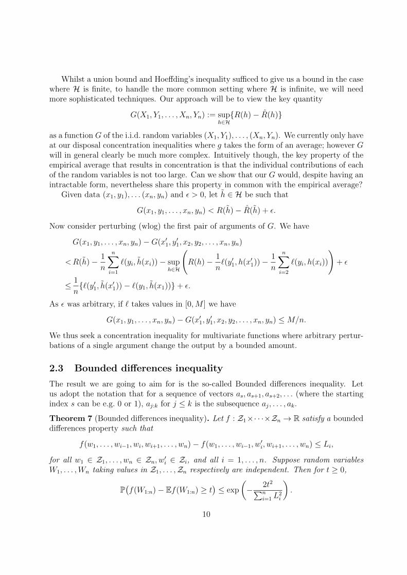
2.3 Bounded differences inequality
The result we are going to aim for is the so-called Bounded differences inequality. Letus adopt the notation that for a sequence of vectors as, as+1, as+2, . . . (where the startingindex s can be e.g. 0 or 1), aj:k for j ≤ k is the subsequence aj, . . . , ak.
Theorem 7 (Bounded differences inequality). Let f : Z1×· · ·×Zn → R satisfy a boundeddifferences property such that
f(w1, . . . , wi−1, wi, wi+1, . . . , wn)− f(w1, . . . , wi−1, w′i, wi+1, . . . , wn) ≤ Li,
for all w1 ∈ Z1, . . . , wn ∈ Zn, w′i ∈ Zi, and all i = 1, . . . , n. Suppose random variablesW1, . . . ,Wn taking values in Z1, . . . ,Zn respectively are independent. Then for t ≥ 0,
P(f(W1:n)− Ef(W1:n) ≥ t
)≤ exp
(− 2t2∑n
i=1 L2i
).
10

Note that when Zi = [ai, bi], taking f(W1:n) =∑
i{Wi −E(Wi)}/n, we recover Hoeffd-ing’s inequality.
To motivate the proof, consider the sequence of random variables given by Z0 =Ef(W1:n), Zn = f(W1:n) and
Zi = E(f(W1:n) |W1:i
)for i = 1, . . . , n− 1.
Note that in the special case where f(W1:n) =∑
iWi and EWi = 0, we have Zk − Z0 =∑ki=1 Wi. Our approach centres on the telescoping decomposition
f(W1:n)− Ef(W1:n) = Zn − Z0 =n∑i=1
(Zi − Zi−1)︸ ︷︷ ︸Di
; (2.5)
the differences Di play an analogous role to the individual independent random variablesin the case of bounding sums. In fact, they are an example of a martingale differencesequence4:
Definition 2. A sequence of random variables D1, . . . , Dn ∈ R is a martingale differencesequence with respect to another sequence of random variables W0, . . . ,Wn, if for i =1, . . . , n,
(i) E|Di| <∞,
(ii) Di is a function of W0:i,
(iii) E(Di |W0:(i−1)) = 0.
Example. If D1, . . . , Dn are independent, mean zero, and satisfy (i), the sequence is amartingale difference sequence with respect to c,D1, . . . , Dn, for arbitrary constant c. 4
Example. The sequence D1, . . . , Dn defined in (2.5) is a martingale difference sequencewith respect to c,W1, . . . ,Wn for arbitrary constant c. That (ii) holds is clear. (i) certainlyholds when f is bounded. That (iii) holds follows from the tower property of conditionalexpectation. 4
We are now in a position to prove a generalisation of Proposition 4 applicable to(weighted) averages of martingale differences.
Lemma 8. Let D1, . . . , Dn be a martingale difference sequence with respect to W0, . . . ,Wn
such thatE(eαDi |W0:(i−1)) ≤ eα
2σ2i /2 i = 1, . . . , n.
Let γ ∈ Rn and write D = (D1, . . . , Dn)T . Then γTD is sub-Gaussian with parameter
(∑
i γ2i σ
2i )
1/2.
4For a more general and formal definition, see Part II Stochastic Financial Models.
11

Proof. We have
E exp(α
n∑i=1
γiDi
)= EE
{exp
(α
n∑i=1
γiDi
) ∣∣W0:(n−1)
}= E
{exp
(α
n−1∑i=1
γiDi
)E(eαγnDn |W0:(n−1))
}≤ eα
2γ2nσ2n/2E exp
(αn−1∑i=1
γiDi
)≤ exp
(α2
2
n∑i=1
γ2i σ
2i
)(arguing inductively).
The Azuma-Hoeffding inequality specialises the above result to the case of boundedrandom variables.
Theorem 9 (Azuma–Hoeffding). Let D1, . . . , Dn be a martingale difference sequence withrespect to W0, . . . ,Wn. Suppose that the following holds for each i = 1, . . . , n: there existrandom variables Ai and Bi that are functions of W0:(i−1) such that Ai ≤ Di ≤ Bi, andBi − Ai ≤ Li for a constant Li. Then for t ≥ 0,
P
(n∑i=1
Di ≥ t
)≤ exp
(− 2t2∑n
i=1 L2i
). (2.6)
Proof. Conditional on W0:(i−1), Ai and Bi are constant. Thus we may apply Hoeffding’slemma (Lemma 3) conditionally on W0:(i−1) to obtain
E(eαDi |W0:(i−1)) ≤ eα2(Li/2)2/2 almost surely.
The martingale difference sequence thus satisfies the hypotheses of Lemma 8. The sum∑iDi is sub-Gaussian with parameter σ = (
∑i L
2i )
1/2/2. The result then follows from the
sub-Gaussian tail bound (Proposition 2).
We are finally ready to prove the Bounded differences inequality.
Proof of Theorem 7. It is convenient to introduce W0 ≡ w0 for an arbitrary constant w0
and treat f as a function f : Z0 × · · · × Zn where Z0 = {w0}.Let D1, . . . , Dn be as in (2.5), so for i = 1, . . . , n
Di = E(f(W0:n) |W0:i
)− E
(f(W0:n) |W0:(i−1)
).
Recall that f(W0:n)− Ef(W0:n) =∑n
i=1Di.Using the Azuma–Hoeffding inequality, it suffices to prove that Ai ≤ Di ≤ Bi almost
surely where Ai and Bi are functions of W0:(i−1) satisfying Bi−Ai ≤ Li for all i, which wenow do.
12

Let us define for each i = 1, . . . , n, functions
Fi : Z0 × · · · × Zi → R(w0, . . . , wi) 7→ E(f(W0:n) |W0 = w0, . . . ,Wi = wi),
so Di = Fi(W0:i)− Fi−1(W0:(i−1)). Then define the random variables
Ai := infwi∈Zi
Fi(W0:(i−1), wi)− Fi−1(W0:(i−1))
Bi := supwi∈Zi
Fi(W0:(i−1), wi)− Fi−1(W0:(i−1)),
so Ai and Bi are functions of W0:(i−1). Then
Di − Ai = Fi(W0:i)− infwi∈Zi
Fi(W0:(i−1), wi) ≥ 0
Di −Bi = Fi(W0:i)− supwi∈Zi
Fi(W0:(i−1), wi) ≤ 0,
so Ai ≤ Di ≤ Bi. Also
Bi − Ai = supwi∈Zi
Fi(W0:(i−1), wi)− infwi∈Zi
Fi(W0:(i−1), wi)
= supwi,w′i∈Zi
{Fi(W0:(i−1), wi)− Fi(W0:(i−1), w′i)}
= supwi,w′i∈Zi
{E(f(W0:(i−1), wi,W(i+1):n) |W0:(i−1),Wi = wi
)− E
(f(W0:(i−1), w
′i,W(i+1):n) |W0:(i−1),Wi = w′i
)}.
Now as the W0:n are independent, the distribution of W(i+1):n conditional on W0:(i−1) andthat conditional on W0:i are identical, so
Bi − Ai = supwi,w′i∈Zi
[E{f(W0:(i−1), wi,W(i+1):n)− f(W0:(i−1), w
′i,W(i+1):n)︸ ︷︷ ︸
≤Li
|W0:(i−1)
}]≤ Li.
We have verified all the conditions of the Azuma–Hoeffding inequality which may now beapplied to give the result.
Note that from the proof above and that of the Azuma–Hoeffding inequality, we seethat f(W0:n) is a sub-Gaussian random variable with parameter σ = (
∑i L
2i )
1/2/2.
2.4 Rademacher complexity
Recall our setup: H is a (now possibly infinite) hypothesis class, ` takes values in [0,M ]are we are aiming to bound the right-hand side of
R(h)−R(h∗) ≤ G+ R(h∗)−R(h∗).
13
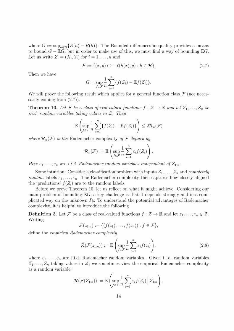
where G := suph∈H{R(h) − R(h)}. The Bounded differences inequality provides a meansto bound G− EG, but in order to make use of this, we must find a way of bounding EG.Let us write Zi = (Xi, Yi) for i = 1, . . . , n and
F := {(x, y) 7→ −`(h(x), y) : h ∈ H}. (2.7)
Then we have
G = supf∈F
1
n
n∑i=1
{f(Zi)− Ef(Zi)}.
We will prove the following result which applies for a general function class F (not neces-sarily coming from (2.7)).
Theorem 10. Let F be a class of real-valued functions f : Z → R and let Z1, . . . , Zn bei.i.d. random variables taking values in Z. Then
E
(supf∈F
1
n
n∑i=1
{f(Zi)− Ef(Zi)}
)≤ 2Rn(F)
where Rn(F) is the Rademacher complexity of F defined by
Rn(F) := E
(supf∈F
1
n
n∑i=1
εif(Zi)
).
Here ε1, . . . , εn are i.i.d. Rademacher random variables independent of Z1:n.
Some intuition: Consider a classification problem with inputs Z1, . . . , Zn and completelyrandom labels ε1, . . . , εn. The Rademacher complexity then captures how closely alignedthe ‘predictions’ f(Zi) are to the random labels.
Before we prove Theorem 10, let us reflect on what it might achieve. Considering ourmain problem of bounding EG, a key challenge is that it depends strongly and in a com-plicated way on the unknown P0. To understand the potential advantages of Rademachercomplexity, it is helpful to introduce the following.
Definition 3. Let F be a class of real-valued functions f : Z → R and let z1, . . . , zn ∈ Z.Writing
F(z1:n) := {(f(z1), . . . , f(zn)) : f ∈ F},define the empirical Rademacher complexity
R(F(z1:n)) := E
(supf∈F
1
n
n∑i=1
εif(zi)
), (2.8)
where ε1, . . . , εn are i.i.d. Rademacher random variables. Given i.i.d. random variablesZ1, . . . , Zn taking values in Z, we sometimes view the empirical Rademacher complexityas a random variable:
R(F(Z1:n)) := E
(supf∈F
1
n
n∑i=1
εif(Zi)∣∣∣Z1:n
).
14

Note that R(F(z1:n)) is well-defined in that the right-hand side of (2.8) only dependson F(z1:n), the ‘behaviours’ of the functions in F on the fixed set of points z1:n.
Key point: R(F(z1:n)) does not depend on P0. It is conceivable that we could obtainuseful upper bounds of R(F(z1:n)) that are uniform in z1:n ∈ Zn. We then immediatelyget a bound on Rn(F) = E{R(F(Z1:n))} that is independent of P0.
Below we summarise some useful properties of Rademacher complexity. Let F1, . . . ,Fm beclasses of functions f : Z → D ⊆ R.
(i) If G = {f1 + f2 : f1 ∈ F1, f2 ∈ F2}, then Rn(G) = Rn(F1) +Rn(F2).
(ii) If D = [0,M ], then Rn(∪mj=1Fj) ≤ maxj=1,...,mRn(Fj) +M√
2 log(m)/n.
We now turn to the proof of Theorem 10, which uses a symmetrisation technique.
Proof of Theorem 10. Let us introduce an independent copy (Z ′1, . . . , Z′n) of (Z1, . . . , Zn).
We have
supf∈F
1
n
n∑i=1
{f(Zi)− Ef(Zi)} = supf∈F
1
n
n∑i=1
E{f(Zi)− f(Z ′i) |Z1:n} (independence of Z1:n and Z ′1:n)
≤ E
(supf∈F
1
n
n∑i=1
{f(Zi)− f(Z ′i)}∣∣∣∣Z1:n
).
Note we have used the fact that for any collection of random variables Vt, supt′ EVt′ ≤E supt Vt; this may easily be verified by removing the supremum over t′ and noting thatthe resulting inequality must hold for all t′. Now let ε1, . . . , εn be i.i.d. Rademacher randomvariables, independent of Z1:n and Z ′1:n. Then
supf∈F
1
n
n∑i=1
{f(Zi)− f(Z ′i)}d= sup
f∈F
1
n
n∑i=1
εi{f(Zi)− f(Z ′i)}
≤ supf∈F
1
n
n∑i=1
εif(Zi) + supg∈F
1
n
n∑i=1
{−εig(Zi)}.
Noting that ε1:nd= −ε1:n, we have
E
(supf∈F
1
n
n∑i=1
{f(Zi)− f(Z ′i)}
)≤ E
(supf∈F
2
n
n∑i=1
εif(Zi)
)= 2Rn(F).
Theorem 11 (Generalisation bound based on Rademacher complexity). Let F := {(x, y) 7→`(h(x), y) : h ∈ H} and suppose ` takes values in [0,M ]. With probability at least 1− δ,
R(h)−R(h∗) ≤ 2Rn(F) +M
√2 log(2/δ)
n.
15

Proof. Let G := suph∈H{R(h)− R(h)} and recall that
R(h)−R(h∗) ≤ G+ R(h∗)−R(h∗) = (G− EG) + EG+ R(h∗)−R(h∗).
Further recall that viewing G as a function of Z1, . . . , Zn where Zi = (Xi, Yi), it satisfiesa bounded differences property with constants Li = M/n. Thus the Bounded differencesinequality gives us that
P(G− EG ≥ t/2) ≤ exp(−t2n/(2M2)).
Hoeffding’s inequality (or Bounded differences with the average function) also gives P(R(h∗)−R(h∗) ≥ t/2) ≤ exp(−t2n/(2M2)). Also, noting thatRn(F) = Rn(−F), from Theorem 10,EG ≤ 2Rn(F). Thus taking t = M
√2 log(2/δ)/n gives the result.
2.5 VC dimension
All we need to do in order to bound the generalisation error is to obtain bounds on theRademacher complexity. There are various ways of tackling this problem in general. Here,we will explore an approach suited to the classification setting with misclassification lossand F := {(x, y) 7→ `(h(x), y) : h ∈ H}. Our bounds will be in terms of the number ofbehaviours |F(z1:n)| of the function class F on n points z1:n. Observe first that |F(z1:n)| =|H(x1:n)| where zi = (xi, yi).
Lemma 12. We have R(F(z1:n)) ≤√
2 log(|F(z1:n)|)/n =√
2 log(|H(x1:n)|)/n.
Proof. Let d = |F(z1:n)| and let F ′ := {f1, . . . , fd} be such that F(z1:n) = F ′(z1:n) (so eachfj has a unique behaviour on z1:n). For j = 1, . . . , d, let
Wj =1
n
n∑i=1
εifj(zi),
where ε1:n are i.i.d. Rademacher random variables. Then R(F(z1:n)) = EmaxjWj. ByLemma 3 and Proposition 4, each Wj is sub-Gaussian with parameter 1/
√n. Thus we may
apply Proposition 5 on the expected maximum of sub-Gaussian random variables to givethe result.
As each h(xi) ∈ {−1, 1}, we always have |H(x1:n)| ≤ 2n. Considering the result above,an interesting case then is when |H(x1:n)| is growing slower than exponentially in n, e.g.growing polynomially in n.
Definition 4. Let F be a class of functions f : X → {a, b} with a 6= b (e.g. {a, b} ={−1, 1}) with |F| ≥ 2.
� We say F shatters x1:n ∈ X n if |F(x1:n)| = 2n.
� Define also s(F , n) := maxx1:n∈Xn |F(x1:n)|; this is known as the shattering coefficient.
16

� The VC dimension VC(F) is the largest integer n such that some x1:n is shatteredby F , or ∞ if no such n exists. Equivalently, VC(F) = sup{n ∈ N : s(F , n) = 2n}.
Example. Let X = R and consider F = {fa,b : fa,b(x) = 1[a,b)(x) : a, b,∈ R}. Con-sider n distinct points x1, . . . , xn. These divide up the real line into n + 1 intervals(−∞, x1], (x1, x2], . . . , (xn−1, xn], (xn,∞). Now if a and a′ are in the same interval, andb and b′ are in the same interval, then (fa,b(xi))
ni=1 = (fa′,b′(xi))
ni=1. Thus every possible
behaviour (fa,b(xi))ni=1 can be obtained by picking one of the n + 1 intervals for each of a
and b, sos(F , n) ≤ (n+ 1)2.
Now consider VC(F). Any x1:2 can be shattered, but with three points x1 < x2 < x3, wecan never have f(x1) = f(x3) = 1 but f(x2) = 0. Thus VC(F) = 2. 4
It is a bit tedious to determine the shattering coefficient individually for each F andsee whether it grows polynomially; we would like a more streamlined approach. Observethat in the previous example, we have s(F , n) ≤ (n + 1)VC(F). The usefulness of the VCdimension, named after its inventors Vladmir Vapnik and Alexey Chervonenkis, is due tothe remarkable fact that this is true more generally. The result below is known as theSauer–Shelah lemma.
Lemma 13 (Sauer–Shelah). Let F be a class with finite VC dimension d. Then
s(F , n) ≤d∑i=0
(n
i
)≤ (n+ 1)d.
What is striking about this result is that whilst we know from the definition that for alln > d, s(F , n) < 2n, it is not immediately obvious that we cannot have s(F , n) = 2n − 1,or s(F , n) = 1.8n for n > d. The result shows that beyond d the growth of s(F , n) isradically different in that it is polynomial. The important consequence of this is that fromLemma 12 we have
Rn(F) ≤√
2VC(F) log(n+ 1)
n.
*Proof of Lemma 13*. We will prove the following stronger result. Fix x1:n ∈ X n and let xQfor any non-empty Q = {i1, . . . , i|Q|} ⊆ {1, . . . , n} be (xi1 , . . . , xi|Q|). Then we claim that thereare at least |F(x1:n)| − 1 non-empty sets Q ⊆ {1, . . . , n} such that F shatters xQ.
That this implies the statement of the lemma may be seen from the following reasoning. Takex1:n to be such that |F(x1:n)| = s(F , n). As VC(F) = d, by definition no xQ with |Q| > d canbe shattered, so from the claim,
|F(x1:n)| − 1 ≤ (# of shattered sets xQ) ≤d∑i=1
(n
i
).
It remains to prove the claim, which we do by induction on |F(x1:n)|. Wlog assume thefunctions in F map to {−1, 1}. The claim when |F(x1:n)| = 1 is clearly true (the statement
17

is vacuous in this case). Now take k ≥ 1 and suppose the result is true for all n ∈ N andx1:n ∈ X n and F with |F(x1:n)| ≤ k. We will show the result holds at k + 1. Take any n ∈ N,x1:n ∈ X n and F with |F(x1:n)| = k + 1. Let xj be such that F+ := {f ∈ F : f(xj) = 1} andF− := {f ∈ F : f(xj) = −1} are both non-empty (which is possible as |F(x1:n)| ≥ 2). Then
|F+(x1:n)|+ |F−(x1:n)| = |F(x1:n)| = k + 1.
Let X− and X+ be the sets of subvectors xQ that are shattered by F− and F+ respectively.By the induction hypothesis, |X−|+ |X+| ≥ k− 1. Clearly if xQ ∈ X− ∪X+, xQ can be shatteredby F ⊃ F1,F+. Now none of the subvectors in X− ∪ X+ can have xj as a component as thenthe subvector could not be shattered (each subfamily of hypotheses has all f(xj) taking the samevalue). But then when xQ ∈ X− ∩ X+, it must be the case that both xQ and xQ∪{j} (which aredistinct) can be shattered by F . Also xj itself is shattered by F . Thus we see that the numberof sets shattered by F is at least
1 + |X− ∪ X+|+ |X− ∩ X+| = 1 + |X−|+ |X+| ≥ 1 + (k − 1) = k,
thereby completing the induction step.
Example. Let X = Rp and consider F = {1A : A ∈ A} where A ={∏p
j=1(−∞, aj] :
a1, . . . , ap ∈ R}
. To compute VC(F), first note that the set of standard basis vectorse1, . . . , ep ∈ Rp is shattered as for any I ⊆ {1, . . . , p}, we may take aj = 1 if j ∈ I andaj = 0 otherwise; then
ej ∈p∏
k=1
(−∞, ak] ⇔ j ∈ I.
Next take x1, . . . , xp+1 ∈ Rp. For each coordinate j = 1, . . . , p, let Jj = {k : xkj =maxl xlj}. Then there must be some xk∗ such that k∗ is not a unique element of one ofthe Jj. But then for each j = 1, . . . , p, there exists some xkj such that xkjj ≥ xk∗j, so forf ∈ F we can never have f(xk∗) = 0 and f(xk) = 1 for all k 6= k∗. Thus VC(F) = p. 4
An important class of hypotheses H is based on functions that form a vector space.Let F be a vector space of functions f : X → R, e.g. consider X = Rp and
F = {x 7→ xTβ : β ∈ Rp}.
From F form a class of hypotheses
H = {h : h(x) = sgn(f(x)) where f ∈ F}. (2.9)
The following Proposition bounds the VC dimension of H.
Proposition 14. Consider hypothesis class H given by (2.9) where F is a vector space offunctions. Then
VC(H) ≤ dim(F).
18

Proof. Let d = dim(F) + 1 and take x1:d ∈ X d. We need to show that x1:d cannot beshattered by H. Consider the linear map L : F → Rd given by
L(f) = (f(x1), . . . , f(xd)) ∈ Rd.
The rank of L is at most dim(F) = d−1 < d. Therefore, there must exist non-zero γ ∈ Rd
orthogonal to everything in the image L(F) i.e.∑i:γi>0
γif(xi) +∑i:γi≤0
γif(xi) = 0 for all f ∈ F , (2.10)
where wlog at least one component of γ is strictly positive. Let I+ = {i : γi > 0} andI− = {i : γi ≤ 0}. Then it is not possible to have
h(xi) = 1⇒ f(xi) > 0 for all i ∈ I+,
h(xi) = −1⇒ f(xi) ≤ 0 for all i ∈ I−,
(recall we are taking sgn(0) := −1) as otherwise the LHS of (2.10) would be strictlypositive. Thus x1:d cannot be shattered so VC(H) ≤ d− 1 as required.
3 Computation for empirical risk minimisation
The results of the previous section have given us a good understanding of the theoreticalproperties of the ERM h corresponding to a given hypothesis class. We have not yetdiscussed whether h can be computed in practice, and how to do so; these questions arethe topic of this chapter.
For a general hypothesis class H, computation of the ERM h can be arbitrarily hard.Things simplify greatly if computing h may be equivalently phrased in terms of minimisinga convex function over a convex set.
3.1 Basic properties of convex sets
Recall that a set C ⊆ Rd is convex if
x, y ∈ C ⇒ (1− t)x+ ty ∈ C for all t ∈ (0, 1).
The intersection of an arbitrary collection of convex sets is convex, so if for each α ∈ I,the set Cα ∈ Rd is convex, then ∩α∈ICα is convex (see Example Sheet 2).
Definition 5. .
� For a set S ⊆ Rd, the convex hull convS is the intersection of all convex sets con-taining S.
19

� A point v ∈ Rd is a convex combination of v1, . . . , vm ∈ Rd if
v = α1v1 + · · ·+ αmvm
where α1, . . . , αm ≥ 0 and∑m
j=1 αj = 1.
Lemma 15. For S ⊆ Rd, v ∈ convS if and only if v is a convex combination of some setof points in S.
Proof. Let D be the set of all convex combinations of sets of points from S. We want toshow D ⊇ convS and D ⊆ convS. Showing the former is a task on Example Sheet 2; weshow the latter relation D ⊆ convS.
Now intersections of convex sets are convex, so convS is convex. Thus clearly a convexcombination of any v1, v2 ∈ S is in convS. Suppose then that for m ≥ 2, any convexcombination of m points from S is in convS. Take v1, . . . , vm+1 ∈ S and α1, . . . , αm+1 ≥ 0with
∑m+1j=1 αj = 1. Consider v =
∑m+1j=1 vjαj. If αm+1 = 1, v = vm+1 ∈ S ⊆ convS.
Otherwise, writing t =∑m
j=1 αj, we have t > 0 and αm+1 = 1− t so
v = t( α1
tv1 + · · ·+ αm
tvm︸ ︷︷ ︸
∈ convS by theinduction hypothesis
)+ (1− t)vm+1 ∈ convS.
Lemma 16. Let S ⊆ Rd. For any linear map L : Rd → Rn, convL(S) = L(convS).
Proof. u ∈ convL(S) iff. there exist v1, . . . , vm ∈ S and α1, . . . , αm ≥ 0 such that∑m
j=1 αj =1 and
u =∑j
αjL(vj).
But the RHS is L(∑
j αjvj
)∈ L(convS) and u ∈ L(convS) iff. u takes this form.
3.2 Basic properties of convex functions
In the following, let C ⊆ Rd be a convex set. A function f : C → R is convex if
f((1− t)x+ ty
)≤ (1− t)f(x) + tf(y) for all x, y ∈ C and t ∈ (0, 1).
Then −f is a concave function. It is strictly convex if the inequality is strict for all x, y ∈ C,x 6= y and t ∈ (0, 1).
Convex functions exhibit a “local to global phenomenon”: for example local minimaare necessarily global minima. Indeed, if x ∈ C is a local minimum, so for all y ∈ C,f((1− t)x+ ty) ≥ f(x) for all t sufficiently small, then by convexity
f(x) ≤ f((1− t)x+ ty) ≤ (1− t)f(x) + tf(y),
20

so f(x) ≤ f(y) for all y ∈ C. On the other hand, non-convex functions can have manylocal minima whose objective values are far from the global minimum, which can makethem very hard to optimise.
We collect together several useful properties of convex functions in the following propo-sition.
Proposition 17. In the following, let C ⊆ Rd be a convex set and let f : C → R be aconvex function, unless specified otherwise.
New convex functions from old:
(i) Let g : C → R be a (strictly) convex function. Then if a, b > 0, af + bg is a (strictly)convex function.
(ii) Let A ∈ Rd×m and b ∈ Rd and take C = Rd. Then g : Rm → R given by g(x) =f(Ax− b) is a convex function.
(iii) Suppose fα : C → R is convex for all α ∈ I where I is some index set, and defineg(x) := supα∈I fα(x). Then
(a) D := {x ∈ C : g(x) <∞} is convex and
(b) function g restricted to D is convex.
Consequences of convexity:
(iv) If f is differentiable at x ∈ int(C) then f(y) ≥ f(x) +∇f(x)T (y − x) for all y ∈ C.In particular, ∇f(x) = 0⇒ x minimises f .
(v) If f is a strictly convex function, then any minimiser is unique.
(vi) If C = convD, then supx∈C f(x) = supx∈D f(x).
Checking convexity:
(vii) If f : Rd → R is twice continuously differentiable then
(a) f is convex iff. its Hessian matrix H(x) at x is positive semi-definite for all x,
(b) f is strictly convex if H(x) is positive definite for all x.
3.3 Convex surrogates
In the classification setting, one problem with using misclassification loss is that the ERMoptimisation can be intractable for many hypothesis classes. For example, taking H basedon half-spaces, the ERM problem minimises over β ∈ Rp the following objective:
n∑i=1
1{sgn(XTi β)6=Yi} ≈
n∑i=1
1(−∞,0](YiXTi β)
21

−1.5 −1.0 −0.5 0.0 0.5 1.0 1.5
0.0
0.5
1.0
1.5
2.0
2.5
3.0
u
φ(u
)
0−1 losshinge losslogistic lossexponential loss
(ignoring when XTi β = 0). The RHS is not convex and in fact not continuous due to
the indicator function. If 1(−∞,0] above were somehow replaced with a convex function,we know from Proposition 17 (i) & (ii) that the resulting objective would be a convexfunction of β. The minimising β may still be able to deliver classification performance viax 7→ sgn(xT β) that is comparable to that of the ERM provided the convex function is asufficiently good approximation to an indicator function.
These considerations motivate the following changes to the classification frameworkthat we have been studying thus far.
� Rather than performing ERM over a set of classifiers, let us consider a family H offunctions h : X → R. Each h ∈ H determines a classifier via x 7→ sgn(h(x)).
� We will consider loss functions ` : R× R→ [0,∞) of the form
`(h(x), y) = φ(yh(x))
and φ : R → [0,∞) is convex. We will refer to the corresponding risk as the φ-riskand denote it by Rφ. Note formally we will be taking Y = R (even though the data(Yi)
ni=1 are in {−1, 1}).
Common choices of φ include the following:
� Hinge loss: φ(u) = max(1− u, 0).
� Exponential loss: φ(u) = e−u.
� Logistic loss: φ(u) = log2(1 + e−u) = log(1 + e−u)/ log(2).
For the strategy of using a surrogate loss to be useful, ERM with the surrogate loss shouldhopefully mimic using misclassification loss. For example, we would ideally like the hφ,0that minimises Rφ (assuming it exists) to be such that x 7→ sgn(hφ,0(x)) is (equivalent to)
22

the Bayes classifier x 7→ sgn(η(x)−1/2). To understand when this is the case, we introducethe following definitions.
The conditional φ-risk of h is
E(φ(Y h(X))|X = x) = η(x)φ(h(x)) + (1− η(x))φ(−h(x)),
where recall η(x) = P(Y = 1|X = x). It will be helpful to consider this in terms of a genericconditional probability η ∈ [0, 1] and generic value α ∈ R of h(x). We thus introduce
Cη(α) := ηφ(α) + (1− η)φ(−α).
The following definition encapsulates our idea of sgn ◦ hφ,0 achieving the optimal Bayesmisclassification risk, but also allows for the possibility that infhRφ(h) is not attained.
Definition 6. We say φ : R → [0,∞) is classification calibrated if for any η ∈ [0, 1] withη 6= 1/2,
infα∈R
Cη(α) < infα:α(2η−1)≤0
Cη(α).
In words, the equation above says that the infimal generic conditional φ-risk is strictlyless than the infimum where α (playing the role of h(x)) is forced to disagree in sign withthe Bayes classifier. The following result tells us when the favourable case of classificationcalibration occurs for convex φ.
Theorem 18. Let φ be convex. Then φ : R → [0,∞) is classification calibrated if it isdifferentiable at 0 and φ′(0) < 0.
Proof. Note that Cη is convex and differentiable at 0 with
C ′η(0) = (2η − 1)φ′(0).
Suppose η > 1/2, so C ′η(0) < 0. Then from Proposition 17 (iv),
Cη(α) ≥ Cη(0) + C ′η(0)α ≥ Cη(0)
for α ≤ 0. Also as
0 > C ′η(0) = limα↓0
Cη(α)− Cη(0)
α,
for some α∗ > 0 we have Cη(α∗) < Cη(0). Similarly when η < 1/2, there exists some α∗ < 0
with Cη(α∗) < Cη(0). Thus in both cases infα∈RCη(α) ≤ Cη(α
∗) < infα:α(2η−1)≤0Cη(α).
We thus see that the popular choices of φ above are all classification calibrated.
23

3.4 Rademacher complexity revisited
One remaining issue is whether we can obtain guarantees on when the generalisation er-ror measured in terms of φ-risk is small. Theorem 11 gives us a bound in terms of theRademacher complexity of
F = {(x, y) 7→ φ(yh(x)) : h ∈ H}.
Our bounds for Rn(F) involving shattering coefficients and VC dimension relied heavilyon the use of misclassification loss. We will need a different approach here. One useful stepwould be to relate Rn(F) to Rn(H) which is potentially simpler to handle. The followingresult, which is sometimes known as the contraction lemma, helps in this regard.
Lemma 19 (Contraction lemma). Let r = supx∈X ,h∈H |h(x)|. Suppose there exists L ≥ 0with |φ(u)− φ(u′)| ≤ L|u− u′| for all u, u′ ∈ [−r, r], so φ is Lipschitz with constant L on[−r, r]. Then Rn(F) ≤ LRn(H).
*Proof*. Let (x1, y1), . . . , (xn, yn) ∈ X×{−1, 1} and let ε1, . . . , εn be a sequence of i.i.d. Rademacherrandom variables. Then writing zi = (xi, yi), we have
R(F(z1:n)) = E
(suph∈H
1
n
n∑i=1
εiφ(yih(xi))
).
Let us consider z1:n as fixed and, for any i, write ε−i for the sequence ε1:n with εi removed. Weclaim that for any (suitable) function A : H× {−1, 1}n−1,
E suph∈H
(1
nεiφ(yih(xi)) +A(h, ε−i)
)≤ E sup
h∈H
(L
nεih(xi) +A(h, ε−i)
). (3.1)
Applying this with i = 1 and
A(h, ε−1) =1
n
n∑i=2
εiφ(yih(xi)),
we get
E suph∈H
(1
nε1φ(y1h(x1)) +
1
n
n∑i=2
εiφ(yih(xi))
)≤ E sup
h∈H
(L
nε1h(x1) +
1
n
n∑i=2
εiφ(yih(xi))
). (3.2)
Next applying (3.1) with i = 2 and
A(h, ε−2) =1
n
n∑i=3
εiφ(yih(xi)) +L
nε1h(x1),
we get that the RHS of (3.2) is at most
E suph∈H
(L
n
2∑i=1
εih(xi) +1
n
n∑i=3
εiφ(yih(xi))
).
24

Continuing this argument yields the result. It remains to prove the claim, which we do now. Wehave
E suph∈H
(1
nεiφ(yih(xi)) +A(h, ε−i)
∣∣∣ ε−i)=
1
2n
[suph∈H{φ(yih(xi)) + nA(h, ε−i)}+ sup
h∈H{−φ(yih(xi)) + nA(h, ε−i)}
]=
1
2n
[suph,g∈H
{φ(yih(xi))− φ(yig(xi))︸ ︷︷ ︸≤L|h(xi)−g(xi)|
+nA(h, ε−i) + nA(g, ε−i)}].
But by symmetry,
suph,g∈H
{L|h(xi)− g(xi)|+ nA(h, ε−i) + nA(g, ε−i)}
= suph,g∈H
[L{h(xi)− g(xi)}+ nA(h, ε−i) + nA(g, ε−i)]
= suph∈H{Lh(xi) + nA(h, ε−i)}+ sup
h∈H{−Lh(xi) + nA(h, ε−i)}.
Hence
E suph∈H
(1
nεiφ(yih(xi)) +A(h, ε−i)
∣∣∣ ε−i) ≤ E suph∈H
(L
nεih(xi) +A(h, ε−i)
∣∣∣ ε−i)Taking expectations proves the claim.
Corollary 20. Consider the setup of Lemma 19 and suppose r is finite. Suppose φ isnon-increasing and let M = φ(−r). Then with probability at least 1− δ,
Rφ(h)−Rφ(h∗) ≤ 2LRn(H) +M
√2 log(2/δ)
n.
In order for the result above to be applicable when φ is e.g. one of the convex surrogatesdiscussed earlier, we need H to be such that r is finite so M is finite. This will not holdfor our example where X = Rp of
H = {x 7→ xTβ : β ∈ Rp}.
However, if we constrain the norm of the β and X is a bounded subset of Rp, we canachieve this.
3.5 `2-constraint
Suppose X = {x ∈ Rp : ‖x‖2 ≤ C} and consider
H = {x 7→ xTβ : β ∈ Rp and ‖β‖2 ≤ λ} (3.3)
25

for λ > 0. Then we have that for any x1:n ∈ X n,
R(H(x1:n)) =1
nE
(sup
β:‖β‖2≤λ
n∑i=1
εixTi β
)
≤ λ
nE∥∥∥ n∑i=1
εixi
∥∥∥2
(Cauchy–Schwarz)
≤ λ
n
(E∥∥∥ n∑i=1
εixi
∥∥∥2
2
)1/2
,
where the last inequality follows due to concavity of√· and Jensen’s inequality. Now for
i 6= j, E(εixTi xjεj) = 0, so
E∥∥∥ n∑i=1
εixi
∥∥∥2
2=
n∑i=1
‖xi‖22 ≤ nC2.
ThusR(H(x1:n)) ≤ λC/
√n
Furthermore
supx∈X ,h∈H
|h(x)| = supx:‖x‖2≤C,β:‖β‖2≤λ
xTβ = λC.
Example. Take φ to be the hinge loss and H given by (3.3). Then from Corollary 20,with probability at least 1− δ,
Rφ(h)−Rφ(h∗) ≤ 2λC√n
+ (λC + 1)
√2 log(2/δ)
n.
4
3.6 *Kernel machines*
Consider the optimisation problem solved by the empirical risk minimiser with hypothesis class
H =
{x 7→
d∑j=1
βjϕj(x) : β ∈ Rd and ‖β‖2 ≤ λ}
and data (Xi, Yi)ni=1. Consider now a Lagrangian formulation of the objective, given by
arg minβ:β∈Rd
1
n`(Yi, (Φβ)i) + γ‖β‖22. (3.4)
Here γ > 0 is a Lagrange multiplier, and matrix Φ ∈ Rn×d has Φij = ϕj(xi) (note we have squaredthe `2-norm in the original constraint). If d is large, this can be a challenging optimisation problemto solve.
26

Consider however the projection P ∈ Rd×d onto the row space of Φ, and note that Φβ = ΦPβ.Meanwhile, we have that
‖β‖22 = ‖Pβ‖22 + ‖(I − P )β‖22.We conclude that any minimiser, β, of (3.4) must satisfy β = P β, that is β must be in therow space of Φ. This means that we may write β = ΦT α for some α ∈ Rn. Now let functionk : X × X → R be given by
k(x, x′) =
d∑j=1
ϕj(x)ϕj(x′), (3.5)
and let K ∈ Rn×n be the matrix with ijth entry Kij = k(xi, xj), so K = ΦΦT . Substitutingβ = ΦTα into (3.4), we see that α minimises
1
n`(Yi, (Kα)i) + γαTKα (3.6)
over α ∈ Rn. Note that the empirical risk minimiser evaluated at a point x ∈ X is given by
d∑j=1
ϕj(x)βj =
d∑j=1
ϕj(x)(ΦT α)j =
n∑i=1
k(x, xi)αi.
What is remarkable is that whilst the optimisation in (3.4) involves d variables, we have shownthis is equivalent to (3.6) which involves n variables: this is a substantial simplification if d� n.In fact, these arguments can be generalised to the case where d =∞.5
The function k in (3.5) is known as a (positive-definite) kernel. For certain families of functions(ϕj)
dj=1, this can be computed very fast. For example, consider X ∈ Rp and
(ϕ1(x), . . . , ϕd(x)) = (x1, . . . , xp,
x1x1, . . . , x1xp,
x2x1, . . . , x2xp,
xpx1, . . . , xpxp),
so d = p + p2; note that some functions ϕj occur twice. Naive computation of the resultingk(x, x′) would require summing over O(p2) terms. However note that
k(x, x′) =
p∑j=1
xjx′j +
p∑j=1
p∑k=1
xjxkx′jx′k =
( p∑j=1
xjx′j +
1
2
)2
− 1
4,
which may be found using O(p) computational operations.
3.7 `1-constraint
The `1-norm of a vector u is ‖u‖1 :=∑
i |ui| and the `∞-norm is ‖u‖∞ := maxi |ui|.Suppose now that X = {x ∈ Rp : ‖x‖∞ ≤ C} and consider
H = {x 7→ xTβ : β ∈ Rp and ‖β‖1 ≤ λ}.
To compute the Rademacher complexity of H, we make use of the following.
5This section just scratches the surface of the topic known as kernel machines: see the Part III courseModern Statistical Methods to learn more.
27

Lemma 21. For any A ⊆ Rn, R(A) = R(convA).
Proof. See example sheet.
To use this, observe that if β has ‖β‖1 = λ, then writing
β = λ
p∑j=1
|βj|λ
sgn(βj)ej,
we see that β ∈ convS where S = ∪pj=1{λej,−λej} and ej is the jth standard basis vector.Next if ‖β‖1 ≤ λ, then
β =λ+ ‖β‖1
2λ
λ
‖β‖1
β︸ ︷︷ ︸∈convS
+λ− ‖β‖1
2λ
(−λ)
‖β‖1
β︸ ︷︷ ︸∈convS
∈ convS
as convS is convex. Then given x1, . . . , xn, let L : Rp → Rn be the linear map given by
L(β) = (xT1 β, . . . , xTnβ)T .
Then H(x1:n) = L(convS) = convL(S) from Lemma 16. Thus from Lemma 21 we have
R(H(x1:n)) = R(L(S))
=λ
nE(
maxj=1,...,p
∣∣∣ n∑i=1
εixij
∣∣∣)where ε1, . . . , εn are i.i.d. Rademacher random variables. Now each ±
∑i εixij is sub-
Gaussian with parameter( n∑i=1
x2ij
)1/2
≤ C√n (Proposition 4).
Thus from Proposition 5 we have
R(H(x1:n)) ≤ λ
n× C√n×
√2 log |S| = λC√
n
√2 log(2p).
Also
supx∈X ,h∈H
|h(x)| = supx:‖x‖∞≤C,β:‖β‖1≤λ
xTβ = λC.
Example. Take φ to be the hinge loss and H as above. Suppose X = [−1, 1]p. Then fromCorollary 20, with probability at least 1− δ,
Rφ(h)−Rφ(h∗) ≤ 2λ
√2 log(2p)
n+ (λ+ 1)
√2 log(2/δ)
n.
In contrast, withH given by the `2-constraint (3.3) we would have a bound of order λ√p/n.
Some notable differences are as follows.
28

� The dimension p contributes a factor of order√
log(p) in the `1 constraint case versus√p is the `2 constraint case.
� Write H1 and H2 for the `1 and `2 constrained hypothesis classes with norm con-straints λ1 and λ2 respectively. Suppose that β0 ∈ Rp is such that h0 : x 7→ xTβ0
minimises Rφ over {x 7→ xTβ : β ∈ Rp}.
– If
β0 =
(1√p, . . . ,
1√p
)T,
in order that β0 ∈ H1,H2, we require λ1 ≤√p and λ2 ≥ 1. These choices give
excess risk bounds of order (treating δ as a constant)
`1 :
√p log p
n, `2 :
√p
n.
– If
β0 =( 1√
s, . . . ,
1√s︸ ︷︷ ︸
s of these
, 0, . . . , 0)T,
the corresponding risk bounds would be
`1 :
√s log p
n, `2 :
√p
n.
Conclusion: If every predictor is equally important, the `2 hypothesis class willtend to perform better. If only the s predictors are important and s is small, the `1
approach can perform well.
4
3.8 Projections on to convex sets
Empirical risk minimisation (with a convex surrogate) over the `2 and `1 constraint classesdiscussed above involves minimising a convex function subject to the minimiser being in aconvex set. In order to perform this optimisation it will be helpful to project points on toconvex constraint sets.
Proposition 22. Let C ⊆ Rd be a closed convex set. Then for each x ∈ Rd, the minimiserof ‖x− z‖2 over z ∈ C exists and is unique. Moreover writing
πC(x) = argminz∈C‖x− z‖2,
we have that for all x ∈ Rd,
(x− πC(x))T (z − πC(x)) ≤ 0 for all z ∈ C, (3.7)
‖πC(x)− πC(z)‖2 ≤ ‖x− z‖2 for all z ∈ Rd. (3.8)
29

Proof. Existence: Let µ = infz∈C ‖x− z‖2. Write B = {w : ‖w − x‖2 ≤ µ+ 1}. Then
infz∈C‖x− z‖2 = inf
z∈C∩B‖x− z‖2,
and the RHS is an infimum of a continuous function on a closed and bounded set, so theinfimum is achieved at π = πC(x), say.Uniqueness: For each fixed x, z 7→ ‖x−z‖2
2 is a strictly convex function, so any minimiserover the convex set C must be unique (see example sheet).(3.7): We have (1− t)π + tz ∈ C for all t ∈ [0, 1], so
‖x− π‖22 ≤ ‖x− π + t(π − z)‖2
2
= ‖x− π‖22 − 2t(x− π)T (z − π) + t2‖π − z‖2
2,
whence
(x− π)T (z − π) ≤ t
2‖π − z‖2
2 for all t ∈ (0, 1].
Letting t→ 0 shows (3.7).(3.8): From (3.7) we have
(x− πC(x))T (πC(z)− πC(x)) ≤ 0
(z − πC(z))T (πC(x)− πC(z)) ≤ 0.
Adding these we have
‖πC(x)− πC(z)‖22 ≤ (πC(x)− πC(z))T (x− z)
≤ ‖πC(x)− πC(z)‖2‖z − x‖2 (Cauchy–Schwarz).
Dividing both sides by ‖πC(x)− πC(z)‖2 thus gives the result.
Definition 7. We call πC(x) above the projection of x on C.
3.9 Subgradients
For a convex function f : Rd → R differentiable at x ∈ Rd, we have that
f(z) ≥ f(x) +∇f(x)T (z − x) for all z ∈ Rd,
so in particular there is a hyperplane passing through (x, f(x)) that lies below the function.This also holds true more generally at points where f may not be differentiable with ∇f(x)above replaced by a subgradient.
Definition 8. A vector g ∈ Rd is a subgradient of a convex function f : Rd → R at x if
f(z) ≥ f(x) + gT (z − x) for all z ∈ Rd.
The set of subgradients of f at x is called the subdifferential of f at x and denoted ∂f(x).
30

Proposition 23. If f : Rd → R is convex, ∂f(x) is non-empty for all x ∈ Rd.
*Proof*. The set C = {(z, y) ∈ Rd × R : y ≥ f(z)} (known as the epigraph of f) is closed andconvex. Take a sequence w1, w2, . . . ∈ Rd+1 such that wk /∈ C for each k and wk → (x, f(x)) ask →∞. Then for each k, there exists vk ∈ Rd+1 where
vTk w < vTk wk for all w ∈ C. (3.9)
Indeed taking vk = wk−πC(wk), from Proposition 22, we have that vTk (w−πC(wk)) ≤ 0, so then
vTk w ≤ vTk πC(wk) = vkwk − ‖vk‖22 < vkwk.
We can rescale the vk such that ‖vk‖2 = 1, and (3.9) will be maintained. With this modification,we have that the sequence vk lies in the closed unit ball. Thus by the Bolzano–Weierstrasstheorem, there exists a convergent subsequence vkj → v = (−g, α) as j →∞. Then in particular
−gT z + αy ≤ −gTx+ αf(x) for all (z, y) ∈ C.
Clearly this is only possible if α < 0, so dividing by −α and setting g = g/α and y = f(z) weobtain
f(z) + gT z ≥ f(x) + gTx for all z.
To compute subgradients, the following facts will be helpful.
Proposition 24. Let f : Rd → R be convex, and suppose f is differentiable at x. Then∂f(x) = {∇f(x)}.
Proof. Suppose g ∈ Rd is a subgradient of f at x. Then, for any z ∈ Rd, we have
∇f(x)T z = limt↓0
f(x+ tz)− f(x)
t≥ gT z.
In particular, taking z = g−∇f(x), we have ‖∇f(x)− g‖22 ≤ 0, so we must have ∇f(x) =
g.
Proposition 25 (Subgradient calculus). Let f, f1, f2 : Rd → R be convex. Then
(i) ∂(αf)(x) = {αg : g ∈ ∂f(x)} for α > 0,
(ii) ∂(f1 + f2)(x) = {g1 + g2 : g1 ∈ ∂f1(x), g2 ∈ ∂f2(x)}.
Also if h : Rm → R is given by h(x) = f(Ax+ b) where A ∈ Rd×m and b ∈ Rd, then
(iii) ∂h(x) = AT∂f(Ax+ b).
Example. Consider
f(β) =1
n
n∑i=1
max(1− yixTi β, 0).
31

Let φ(u) = max(1− u, 0). Then
∂φ(u) =
{0} if u > 1,
[−1, 0] if u = 1,
{−1} if u < 1.
By Proposition 25 (iii) writing hi(β) = max(1− yixTi β, 0), we have ∂hi(β) = {−yixit : t ∈[0, 1]} when yix
Ti β = 1. From Proposition 25 (i) and (ii), we see that ∂f(β) consists of
sums of the form − 1n
∑ni=1 yixiti where each ti may be 0, 1 or anything in [0, 1] depending
on the value of yixTi β. 4
3.10 Gradient descent
Suppose we wish to minimise a function f that is differentiable at a point β with gradientg = ∇f(β). A first-order Taylor expansion gives f(z) ≈ f(β) + gT (z − β), so for smallη > 0,
minδ:‖δ‖2=1
f(β + ηδ) ≈ f(β) + η minδ:‖δ‖2=1
gT δ.
Thus to minimise the linear approximation of f at β, one should move in the direction ofthe negative gradient.
The procedure of (projected) gradient descent for minimising f over a closed convex setC uses this intuition to produce a sequence of iterates β1, β2, . . . aiming have f(βs) closeto a minimum f(β) for large s.
Algorithm 1 Gradient descent
Input: β1 ∈ C; number of iterations k ∈ N; sequence of positive step sizes (ηs)k−1s=1
for s = 1 to k − 1 doCompute gs ∈ ∂f(βs)zs+1 = βs − ηsgsβs+1 = πC(zs+1)
end forreturn β = 1
k
∑ks=1 βs
Theorem 26. Suppose β is a minimiser of convex function f : Rp → R over a closedconvex set C ⊆ Rp. Suppose supβ∈C ‖β‖2 ≤ R <∞ and supβ∈C supg∈∂f(β) ‖g‖2 ≤ L <∞.
Then if ηs ≡ η = 2R/(L√k), the output β of the gradient descent algorithm above satisfies
f(β)− f(β) ≤ 2LR√k.
32

Proof. We have
f(βs)− f(β) ≤ gTs (βs − β) (definition of subgradient)
= −1
η(zs+1 − βs)T (βs − β)
=1
2η{‖βs − zs+1‖2
2 + ‖βs − β‖22 − ‖zs+1 − β‖2
2}. (3.10)
From Proposition 22, ‖πC(z)− πC(x)‖2 ≤ ‖z − x‖2, so in particular
‖zs+1 − β‖22 ≥ ‖βs+1 − β‖2
2.
Using this and (3.10),
f(βs)− f(β) ≤ 1
2η{η2‖gs‖2
2 + ‖βs − β‖22 − ‖βs+1 − β‖2
2}. (3.11)
Now ‖gs‖2 ≤ L. Also β1 ∈ C, so by the triangle inequality, ‖β1 − β‖22 ≤ 4R2. Thus
summing we get
1
k
k∑s=1
f(βs)− f(β) ≤ ηL2
2+
1
2ηk
(‖β1 − β‖2
2 − ‖βk+1 − β‖22
)≤ ηL2
2+
2R2
ηk.
Taking the minimising η = 2R/(L√k) and using Jensen’s inequality to give f(β) ≤
1k
∑ks=1 f(βs), we get the result.
Example. Consider ERM with hinge loss, X = {x ∈ Rp : ‖x‖2 ≤ C} and the `2-constrained hypothesis class H = {x 7→ xTβ : ‖β‖2 ≤ λ}. Then a subgradient of theobjective function f at β takes the form
g = − 1
n
n∑i=1
yixiti where ti ∈ [0, 1].
Thus ‖g‖2 ≤ C by the triangle inequality. From Theorem 26 we see that the output ofgradient descent with step size η = 2λ/(C
√k) satisfies f(β)− f(β) ≤ 2Cλ/
√k. 4
3.11 Stochastic gradient descent
One issue with gradient descent is that the gradients themselves may be computationallyexpensive to compute: in the case of ERM the gradient is a sum of n terms correspondingto each data point, and so computing the gradient typically involves a sweep over the entiredataset at each iteration.
Stochastic gradient descent can circumvent this issue in the case of minimising convexfunctions of the form f(β) = Ef(β;U), where
33
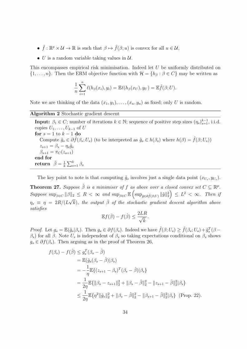
� f : Rp × U → R is such that β 7→ f(β;u) is convex for all u ∈ U ,
� U is a random variable taking values in U .
This encompasses empirical risk minimisation. Indeed let U be uniformly distributed on{1, . . . , n}. Then the ERM objective function with H = {hβ : β ∈ C} may be written as
1
n
n∑i=1
`(hβ(xi), yi) = E`(hβ(xU), yU) = Ef(β;U).
Note we are thinking of the data (x1, y1), . . . , (xn, yn) as fixed; only U is random.
Algorithm 2 Stochastic gradient descent
Input: β1 ∈ C; number of iterations k ∈ N; sequence of positive step sizes (ηs)k−1s=1 , i.i.d.
copies U1, . . . , Uk−1 of Ufor s = 1 to k − 1 do
Compute gs ∈ ∂f(βs;Us) (to be interpreted as gs ∈ h(βs) where h(β) = f(β;Us))zs+1 = βs − ηsgsβs+1 = πC(zs+1)
end forreturn β = 1
k
∑ks=1 βs
The key point to note is that computing gs involves just a single data point (xUs , yUs).
Theorem 27. Suppose β is a minimiser of f as above over a closed convex set C ⊆ Rp.
Suppose supβ∈C ‖β‖2 ≤ R < ∞ and supβ∈C E(
supg∈∂f(β;U) ‖g‖22
)≤ L2 < ∞. Then if
ηs ≡ η = 2R/(L√k), the output β of the stochastic gradient descent algorithm above
satisfies
Ef(β)− f(β) ≤ 2LR√k.
Proof. Let gs = E(gs|βs). Then gs ∈ ∂f(βs). Indeed we have f(β;Us) ≥ f(βs;Us)+ gTs (β−βs) for all β. Note Us is independent of βs so taking expectations conditional on βs showsgs ∈ ∂f(βs). Then arguing as in the proof of Theorem 26,
f(βs)− f(β) ≤ gTs (βs − β)
= E(gs(βs − β)|βs)
= −1
ηE{(zs+1 − βs)T (βs − β)|βs}
=1
2ηE{‖βs − zs+1‖2
2 + ‖βs − β‖22 − ‖zs+1 − β‖2
2|βs}
≤ 1
2ηE{η2‖gs‖2
2 + ‖βs − β‖22 − ‖βs+1 − β‖2
2|βs} (Prop. 22).
34

Taking expectations and summing we get
E
(1
k
k∑s=1
f(βs)
)− f(β) ≤ ηL2
2+
2R2
ηk.
Taking η = 2R/(L√k) and using Jensen’s inequality we get the result.
4 Popular machine learning methods
In the course so far, we have developed a coherent framework giving statistical and compu-tational guarantees for a variety of procedures. However many popular machine learningmethods do not fall precisely within this framework. In this last part of the course, we willbriefly describe a selection of such methods in routine use today. We begin by discussingan important technique for selecting tuning parameters for machine learning methods (e.g.the λ in the cases of `1 and `2-constrained hypotheses), or more generally selecting a goodclassifier or regression method from among a number of competing methods.
4.1 Cross-validation
Let H1, . . . , Hm be a collection of machine learning methods: each Hj takes as its argumenti.i.d. training data (Xi, Yi)
ni=1 =: D and outputs a hypothesis, so Hj
D : X → R. Given aloss function `, we may ideally want to pick a j such that
E{`(HjD(X), Y )|D} (4.1)
is minimised. Here (X, Y ) ∈ X × Y is independent of D and has the same distributionas (X1, Y1). This j is such that conditional on the original training data, it minimises theexpected loss on a new observation drawn from the same distribution as the training data.
A less ambitious goal is to find a j to minimise
E[E{`(HjD(X), Y )|D}] (4.2)
where compared with (4.1), we have taken a further expectation over the training data D.We still have no way of computing (4.2) directly, but we can attempt to estimate it.
The idea of v-fold cross-validation is to split the data into v groups or folds of roughlyequal size. Let D−k be all the data except that in the kth fold, and let Ak ⊂ {1, . . . , n}be the observation indices corresponding to the kth fold. For each j we apply Hj to dataD−k to obtain hypothesis Hj
−k := HjD−k
. We choose the value of j that minimises
CV(j) :=1
n
v∑k=1
∑i∈Ak
`(Hj−k(Xi), Yi). (4.3)
Writing j for the minimiser, we may take final selected hypothesis to be H jD.
35

Note that for each i ∈ Ak,
E`(Hj−k(Xi), Yi) = E[E{`(Hj
−k(Xi), Yi)|D−k}]. (4.4)
This is precisely the expected loss in (4.2) but with training data D replaced with a trainingdata set of smaller size. If all the folds have the same size, then CV(j) is an average ofn identically distributed quantities, each with expected value as in (4.4). However, thequantities being averaged are not independent as they share the same data.
Thus cross-validation gives a biased estimate of the expected prediction error. Theamount of the bias depends on the size of the folds, the case when the v = n giving theleast bias—this is known as leave-one-out cross-validation. The quality of the estimate,though, may be worse as the quantities being averaged in (4.3) will be highly positivelycorrelated. Typical choices of v are 5 or 10.
4.1.1 *Stacking*
Cross-validation aims to allow us to choose the single best machine learning method; we couldinstead aim to find the best weighted combination of methods. To do this, we can attempt tominimise
1
n
v∑k=1
∑i∈Ak
`
m∑j=1
wjHj−k(Xi), Yi
over w in the convex set
{u ∈ Rm : uj ≥ 0 for all j}.
Additional `1 or `2 constraints may be added to the set. This sort of idea is known as stacking
and it can often outperform cross-validation.
4.2 Adaboost
Empirical risk minimisation is a technique for finding a single good hypothesis from a givenhypothesis class. In an analogy with stacking, we could alternatively attempt to find agood weighted combination of hypotheses. Specifically, given an initial set B of classifiersh : X → {−1, 1} such that h ∈ B ⇒ −h ∈ B, consider the class
H =
{M∑m=1
βmhm : βm ≥ 0, hm ∈ B for m = 1, . . . ,M
}.
The class H is clearly richer than B, and the construction above turns out to be useful wayof creating a more complex hypothesis class from a simpler one, with the tuning parameterM controlling the complexity. Performing ERM over H, however, can be computationallychallenging. The Adaboost algorithm can be motivated as a greedy empirical risk min-imisation procedure with exponential loss. As we shall see, one attractive feature of thealgorithm is that it only relies on being able to perform ERM over the simpler class Bgiven different weighted versions of the data.
36

Adaboost first sets f0 to be the function x 7→ 0 and then performs the following form = 1, . . . ,M :
(βm, hm) = arg minβ≥0,h∈B
1
n
n∑i=1
exp[−Yi{fm−1(Xi) + βh(Xi)}]
fm = fm−1 + βmhm.
The final classification is performed according to sgn◦fM . Let us examine the minimisationabove in more detail. Set w
(m)i = n−1 exp(−Yifm−1(Xi)). Then
1
n
n∑i=1
exp[−Yi{fm−1(Xi) + βh(Xi)}] = eβn∑i=1
w(m)i 1{h(Xi)6=Yi} + e−β
n∑i=1
w(m)i 1{h(Xi)=Yi}
= (eβ − e−β)n∑i=1
w(m)i 1{h(Xi)6=Yi} + e−β
n∑i=1
w(m)i .
Provided no h ∈ B perfectly classifies the data so
errm(h) :=
∑ni=1w
(m)i 1{h(Xi)6=Yi}∑ni=1w
(m)i
> 0 for all h ∈ B,
we have thathm = arg min
h∈Berrm(h),
and βm satisfies (eβm + e−βm)errm(hm) = e−βm . Letting x = eβm and a = errm(hm), wehave
(x2 + 1)a = 1
so x =√
1/a− 1
i.e. βm =1
2log
(1− errm(hm)
errm(hm)
).
If M is large, the weighted empirical risk minimisation step to produce the hm must beperformed many times. In order for this approach to be practical, we need B to be suchthat this optimisations can be done very fast. More generally, the hm need not be formedthrough ERM but may be the output of some machine learning method.
Example. Let X = Rp and consider the class of decision stumps
B = {ha,j,1(x) = sgn(xj − a), ha,j,2(x) = sgn(a− xj) : a ∈ R, j = 1, . . . , p}.
To perform weighted ERM with weights w1, . . . , wn > 0 (we have dropped the superscriptm), for each j = 1, . . . , p, first sort {Xij}ni=1 so X(1)j < · · · < X(n)j (we assume these are
37

distinct for simplicity). Fixing j, wlog we may assume X(i)j = Xij = xi. Now observe that(dropping the subscript m),
err(hxk+1,j,1)− err(hxk,j,1) = Yk+1wk+1
/∑l
wl.
Thus picking the optimal ha,j,1 (for fixed j) amounts to picking the minimum across asequence of cumulative sums, and similarly for ha,j,2. This needs to be performed for eachj = 1, . . . , p. Assuming the sorting is performed as part of pre-processing, the weightedempirical risk minimisation has O(np) computational complexity. 4
4.3 Gradient boosting
Consider the following thought experiment. Let us imagine applying gradient descentdirectly to minimise R(h) = E`(h(X), Y ). This would involve the following steps.
1. Start with an initial guess f0 : X → R.
2. For m = 1, . . . ,M , iteratively compute
gm(x) =∂E(`(θ, Y )|X = x)
∂θ
∣∣∣∣fm−1(x)
= E(∂`(θ, Y )
∂θ
∣∣∣fm−1(x)
∣∣∣∣X = x
)assuming sufficient regularity conditions.
3. Update fm = fm−1 − ηgm, where η > 0 is a small step length.
If we want to create a version of the ‘algorithm’ above that works with finite data(X1, Y1), . . . , (Xn, Yn), we need to find a way of approximating the conditional expectationfunction
x 7→ E(∂`(θ, Y )
∂θ
∣∣∣fm−1(x)
∣∣∣∣X = x
).
Recall from (iv) on page 3, that this minimises
E(∂`(θ, Y )
∂θ
∣∣∣fm−1(X)
− h(X)
)2
(4.5)
among all (measurable) functions h : X → R under suitable conditions. This observationmotivates the following algorithm known as gradient boosting, where we try to minimisean empirical version of (4.5) using regression, thereby approximating the conditional ex-pectation. This regression is performed using some base regression method H that takesas its argument some training data D and outputs a hypothesis HD : X → R. In whatfollows, the loss ` may correspond to a convex surrogate or least squares loss for example.
38
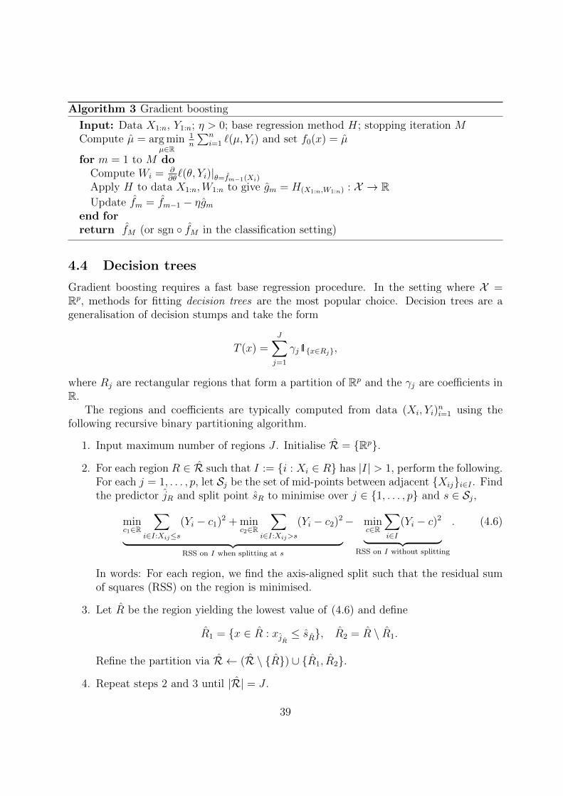
Algorithm 3 Gradient boosting
Input: Data X1:n, Y1:n; η > 0; base regression method H; stopping iteration MCompute µ = arg min
µ∈R
1n
∑ni=1 `(µ, Yi) and set f0(x) = µ
for m = 1 to M doCompute Wi = ∂
∂θ`(θ, Yi)|θ=fm−1(Xi)
Apply H to data X1:n,W1:n to give gm = H(X1:n,W1:n) : X → RUpdate fm = fm−1 − ηgm
end forreturn fM (or sgn ◦ fM in the classification setting)
4.4 Decision trees
Gradient boosting requires a fast base regression procedure. In the setting where X =Rp, methods for fitting decision trees are the most popular choice. Decision trees are ageneralisation of decision stumps and take the form
T (x) =J∑j=1
γj1{x∈Rj},
where Rj are rectangular regions that form a partition of Rp and the γj are coefficients inR.
The regions and coefficients are typically computed from data (Xi, Yi)ni=1 using the
following recursive binary partitioning algorithm.
1. Input maximum number of regions J . Initialise R = {Rp}.
2. For each region R ∈ R such that I := {i : Xi ∈ R} has |I| > 1, perform the following.For each j = 1, . . . , p, let Sj be the set of mid-points between adjacent {Xij}i∈I . Findthe predictor jR and split point sR to minimise over j ∈ {1, . . . , p} and s ∈ Sj,
minc1∈R
∑i∈I:Xij≤s
(Yi − c1)2 + minc2∈R
∑i∈I:Xij>s
(Yi − c2)2
︸ ︷︷ ︸RSS on I when splitting at s
− minc∈R
∑i∈I
(Yi − c)2
︸ ︷︷ ︸RSS on I without splitting
. (4.6)
In words: For each region, we find the axis-aligned split such that the residual sumof squares (RSS) on the region is minimised.
3. Let R be the region yielding the lowest value of (4.6) and define
R1 = {x ∈ R : xjR≤ sR}, R2 = R \ R1.
Refine the partition via R ← (R \ {R}) ∪ {R1, R2}.
4. Repeat steps 2 and 3 until |R| = J .
39
5. Writing R = {R1, . . . , RJ}, let Ij = {i : Xi ∈ Rj} and
γj =1
|Ij|
∑i∈Ij
Yi.
Output T : Rp → R such that T (x) =∑J
j=1 γj1{x∈Rj}.
4.5 Random forests
Whilst decision trees as above are a useful machine learning method in their own right,they are most useful for prediction when used in conjunction with gradient boosting orwithin the Random forest procedure which we now describe.
Consider the regression setting where Yi ∈ R and we are using squared error loss. LetTD be a decision tree trained on data D := (Xi, Yi)
ni=1. Also let T = ETD and let (X, Y ) be
independent of D with (X, Y )d= (X1, Y1). Recall property (iv) on page 3, that for random
variables Z,W ∈ R×W and f :W → R, we have
E{Z − f(W )}2 = E{Z − E(Z |W )}2 + E{E(Z |W )− f(W )}2.
Using this, we have the following decomposition of the expected risk of TD:
ER(TD) = E[{Y − TD(X)}2]
= E{Y − E(Y |X,D)︸ ︷︷ ︸=E(Y |X)
}2 + E{E(Y |X)− TD(X)}2
= EVar(Y |X) + E{TD(X)− E(TD(X) |X)︸ ︷︷ ︸=T (X)
}2 + E{E(Y |X)− T (X)}2
= E{E(Y |X)− T (X)}2︸ ︷︷ ︸squared bias
+EVar(TD(X) |X)︸ ︷︷ ︸variance of the tree
+ EVar(Y |X)︸ ︷︷ ︸irreducible variance
.
If the number of regions J used by TD is large, some of these regions will contain onlysmall numbers of observations in them so the corresponding coefficients γj will by highly
variable and consequently EVar(TD(X) |X) will tend to be large. On the other hand, thesquared bias above and hence R(T ) may be low as a large J would allow T to approximatex 7→ E(Y |X = x) well.
Random forest effectively attempts to ‘estimate’ T and so improve upon the varianceof a single tree. If we had multiple independent datasets D1, . . . , DB, we could form anunbiased estimate via
∑Bb=1 TDb
. Random forest samples the data D with replacement toform new datasets D∗1, . . . , D
∗B and performs the following.
1. For each b = 1, . . . , B, grow a decision tree T (b) := TD∗b but when searching forthe best predictor to split on, randomly sample (without replacement) mtry of the ppredictors and choose the best split from among these variables.
40

2. Output frf = 1B
∑Bb=1 T
(b).
The reason for sampling predictors is to try to make the T (b) more independent. To see whythis would be useful, suppose for b1 6= b2 and some x ∈ Rp that Corr(T (b1)(x), T (b2)(x)) =ρ ≥ 0. Then
Var(frf(x)) =1
BVar(T (1)(x)) +
ρB(B − 1)
B2Var(T (1)(x))
=1− ρB
Var(T (1)(x)) + ρVar(T (1)(x)).
Whilst the first term can be made small for large B, the second term does not dependon B, so we would like ρ to be small. The extra randomisation in the form of samplingpredictors can help to achieve this, and we would expect Var(frf(x)) to decrease with mtry.On the other hand, we would expect the squared bias to increase as mtry is decreased.
4.6 Feedforward neural networks
In recent years, (artificial) neural networks have been shown to be very successful for avariety of learning tasks. The class of feedforward neural networks are based around aparticular class of hypotheses h : X = Rp → R with general form
h(x) = A(d) ◦ g ◦ A(d−1) ◦ g ◦ · · · ◦ g ◦ A(2) ◦ g ◦ A(1)(x)
where
� d is known as the depth of the network;
� A(k)(v) = β(k)v + µ(k) where v ∈ Rmk , β(k) ∈ Rmk+1×mk , µ(k) ∈ Rmk+1 with m1 = pand md+1 = 1;
� g : Rm → Rm applies (for any given m) a so-called activation function ψ : R → Relementwise i.e. for v = (v1, . . . , vm)T , g(v) = (ψ(v1), . . . , ψ(vm))T . The activationfunction is nonlinear and typical choices include
(i) u 7→ max(u, 0) (known as a rectified linear unit (ReLU))
(ii) u 7→ 1/(1 + e−u) (sigmoid).
This cascade of alternating linear and nonlinear compositions can be visualised in the formof a graph. Here we have set h(0) := x and for k = 1, . . . , d − 1, x(k) = A(k)(h(k−1)),h(k) = g(x(k)). The intermediate outputs h(1), . . . , h(d−1) are known as hidden layers andx(d) = A(d)(h(d−1)) = h(x) is sometimes known as the output layer. The parameters(β(k), µ(k))dk=1 are typically fitted to data (x1, y1), . . . , (xn, yn) ∈ Rp × {−1, 1} with empir-ical risk minimisation using a surrogate loss φ. Despite the resulting optimisation beinghighly nonconvex, stochastic gradient descent has been shown empirically to be extremelyeffective in selecting good parameters. A key factor in their success has been the fact that
41

the gradients involved can be computed quickly due to the compositional nature of thehypotheses using the chain rule.
Suppose φ and ψ are differentiable. At an observation (x, y) = (xUs , yUs) we first com-pute all the intermediate quantities h(l) and x(l) given the current values of the parameters.Let z = φ(yh(x)) = φ(yx(d)). We then compute, in order
∂z
x(d)= yφ′(yx(d))
∂z
∂µ(d)=
∂z
x(d),
∂z
∂β(d)1k
=∂z
x(d)h
(d−1)k (4.7)
∂z
∂h(d−1)j
=∂z
∂x(d)β
(d)1j
∂z
∂x(d−1)j
=∂z
∂h(d−1)j
ψ′(x(d−1)j )
∂z
∂µ(d−1)j
=∂z
∂x(d−1)j
,∂z
∂β(d−1)jk
=∂z
∂x(d−1)j
h(d−2)k (4.8)
∂z
∂h(d−2)j
=
md∑k=1
∂z
∂x(d−1)k
β(d−1)kj ,
....
This process is known as back propogation. Note only (4.7) and (4.8) out of the equationspresented above are directly used in the SGD update step; the remaining equations simplyfacilitate computation of the gradient with respect to the (β(k), µ(k))dk=1.
42