Embed Size (px)
Citation preview

mathematics for
economic analysis
BA ECONOMICSII Semester
(2011 Admission)
COMPLEMENTARY COURSE
UNIVERSITY OF CALICUTSCHOOL OF DISTANCE EDUCATION
CALICUT UNIVERSITY.P.O., MALAPPURAM, KERALA, INDIA – 673 635
385
mathematics for
economic analysis
BA ECONOMICSII Semester
(2011 Admission)
COMPLEMENTARY COURSE
UNIVERSITY OF CALICUTSCHOOL OF DISTANCE EDUCATION
CALICUT UNIVERSITY.P.O., MALAPPURAM, KERALA, INDIA – 673 635
385
mathematics for
economic analysis
BA ECONOMICSII Semester
(2011 Admission)
COMPLEMENTARY COURSE
UNIVERSITY OF CALICUTSCHOOL OF DISTANCE EDUCATION
CALICUT UNIVERSITY.P.O., MALAPPURAM, KERALA, INDIA – 673 635
385

School of Distance Education
Mathematics for Economic Analysis-I Page 2
UNIVERSITY OF CALICUT
SCHOOL OF DISTANCE EDUCATION
STUDY MATERIAL
BA ECONOMICS
II Semester (2011 Admission)
COMPLEMENTARY COURSE
MATHEMATICS FOR ECONOMIC ANALYSIS-I
Prepared by:
Module I & IV : Ibrahim.Y.C,Associate Professor in Economics,Govt.College, Kodenchery,Kozhikode – 673 580.
Module II & III: Shabeer.K.P,Assistant Professor in Economics,Govt.College, Kodenchery,Kozhikode – 673 580.
Module V : Rahul.K,Assistant Professorin Economics,N.M.S.M. Government College,Kalpetta, Wayanad – 673 121.
Edited and Scrutinised by
Dr. C.Krishnan,Associate Professor in Economics,Govt.College, Kodenchery,Kozhikode – 673 580.
Layout & Settings
Computer Section, SDE
©
Reserved
School of Distance Education
Mathematics for Economic Analysis-I Page 3
CONTENTS
CHAPTER I THEORY OF SETS 05-16
CHAPTER II FUNDAMENTAL OF LINEAR ALGEBRA-MATRICES 17-28
CHAPTER III MATRIX INVERSION 29-43
CHAPTER IV BASIC MATHEMATICAL CONCEPTS 44-57
CHAPTER V ECONOMIC APPLICATIONS OF GRAPHS & EQUATIONS 58-62

School of Distance Education
Mathematics for Economic Analysis-I Page 4

School of Distance Education
Mathematics for Economic Analysis-I Page 5
CHAPTER ITHEORY OF SETSSet theory plays a vital role in all branches of modern Mathematics and is increasinglyusing in Economics also. The set theory was developed by George Cantor (1845 -1918).A Set is a collection of definite and well distinguished objects. There exist, a rule withthe help of which we are able to say whether a particular object ‘belong to’ the set or ‘doesnot belong to’ the set.Eg:- The Students in a classDays in a monthA team of foot ball playersThe set of positive integersElementsThe Objects in a set or the constituent members of a set are called elements of that set.A set is known by its elements. A set is well defined if and only if it can be decidedthat a given object is an element of the set.Ex: A = {3,5,7,9} is a set of odd numbers 3, 5, 7 and 9, we can say that A is a set of allodd numbers between 1 and 10 or 3, 5, 7, 9 are the elements of A.NotationsIt is convention to denote sets by capital letters A, B, C …………, X, Y, Z …………….. andElements by small letters a, b, c, ………. x, y, z………..If ‘a’ is an element of a set ‘S’, then we denote it as‘a’ is an element of S a ∈ s‘a’ is not an element of S a ∉ sThe symbol ∈ (Epsilon) between ‘a’ and ‘s’ indicates‘a’ is an element of set S‘a’ ‘belong to’ S‘a’ ‘is contained’ in S‘a’ ‘is a member of’ SSimilarly ∉ symbol shows ‘a’ is not an element of set S.Ex. If A = {2, 4, 6, 8} is a set of even number between 1 and 9, then for the element 4, we write4 ∈{2, 4, 6, 8}3∉ {2, 4, 6, 8}

School of Distance Education
Mathematics for Economic Analysis-I Page 6
The element of the sets are separated by commas and written in Braces of FloweredBrackets i.e. {}. An element is never listed twice or more in a set. i.e. repeated elements beingdeleted.Ex. Set of letters in the word ‘good’ is {g, o, d} though ‘good’ has two ‘o’s, only one ‘o’appears in set notation.Method of Representing SetA set can be represented symbolically by three different methods.A. Roster Method or Tabulation Method or Enumeration MethodIf all the elements of a set are known and they are few in numbers we can use RosterMethod for denoting a set. In this method, the elements of the set are written in flowered brackets.Examples:1. A = {a, e, i, o, u}2. B = {2, 4, 8, 16}3. C = { 1, 2, 3, 4, 5}B. Rule Method or Set Builder FormThis method is used when elements of a set have a specific property ‘P’ and if anyobject satisfying the property, x is the element of the set.If ‘x’ is any element of a set ‘A’ having the property ‘p’, then A is denoted asA = {x/x has the property ‘p’}or A = {x:x has the property ‘p’}Hence the vertical line ‘/’ or ‘:’ is read as “such that”Examples:(1) Let ‘A’ be the set of all odd numbers, then it can be expressed asA = {x/x is odd}(2) Set of add numbers less than ‘10’ can be expressed asA = {x:x is an odd number <10}If we express the same thing in Tabular Form we get A = {1, 3, 5, 7, 9}C. Descriptive Phrase MethodThis is a method of expressing a set of elements by stating in words what its elements areExamples:(1) A is a set of first five even numbers(2) The set of first five natural numbersExamples of different methods of representing a setA = {2, 4, 6, 8, 10} Tabular formA = { x:x is an even numbers less than 11} – Set Builder Form.A is a set of first five even numbers – Descriptive Phrase Method

School of Distance Education
Mathematics for Economic Analysis-I Page 7
1.1 KINDS OF SETSA. Finite SetsA set is said to be finite if it consists of a specific numbers or finite number ofelements. The elements of such a set can be counted by a finite numberEx. (1) A = { 1, 2, 3, 4, 5}(2) Set of even numbers between 10 and 20.B. Infinite SetsIf a set contain infinite number of elements, it is a infinite set. The elements of such aset cannot be counted by a finite number.Ex. (1) Set of odd numbers(2) A = { x:x is a number between 0 and 1}C. Null set of Empty set or Zero setA set which does not contain any element is called a null set or empty set.Null set is denoted by ϕ of {}Examples (1) A = {x/x is real number whose square is negative}(2) B = {x/x is a negative number greater than 0}(3) C = {x/x is a child having an age of 70}D. Singleton Set or Unit SetA set containing only one element is called Unit set or singleton set.Ex. (1) Set of Positive integers less than 2(2) A = {5}(3) A = {0}E. Equal Sets or Identical Sets or Equality of SetsTwo sets A and B are equal sets or identical sets if and only if they contain the sameelements i.e. A = B.Ex. (1) If A = {2, 3, 4, 5} B = {4, 2, 5, 3} then A = B(2) A = set of even numbers between 1 and 9B = { 2, 4, 6, 8} the A = BF. SubsetsSubset of a set B is a set which consists of some or all of the elements of B. A set ‘A’ isa ‘sub set’ of set ‘B’ if and only if each element of set ‘A’ is also an element of the set B.We denote it as A⊆B which is read as “A is a subset of B”. a ∈ A implies a∈B or ‘a’contained in B.If A is not a subset of B, we denote this by A⊈B.

School of Distance Education
Mathematics for Economic Analysis-I Page 8
G. Super SetIf A is a subset of B, then we say that B is a ‘Super Set’ of A. We denote this relation as B⊇A.Ex. A = { 2, 3, 4, 5}, B = {1, 2, 3, 4, 5, 6, 7} the A⊆B and B⊆A.H. Proper SubsetSet A is a ‘Proper Subset’ of a set ‘B’, if an only if each element of the set A is anelement of the set B and at least one element of the set B is not an element of the set A. Wedenote this as A⊂B. If A is not a proper subset of B, we denote this by A⊄B.Ex. Let A = {1, 3, 5, 7, 9} B = {1, 2, 3, 4, 5, 6, 7 8, 9}Hence all the elements of set A one also the elements of set B and the elements of the set B i.e.2, 4, 6, 8, are not the elements of set A, so A⊂B.1. Improper SubsetA set ‘A’ is called an ‘Improper Subset of set B’ if and only if A=B i.e. every set is“Improper subset of itself”Ex. A = {1, 2, 3, 4} B = {4, 3, 2, 1}. Hence A=B, therefore A is improper subset of B.J. Universal SetAny set under discussion can be treated as a subset of a big set. This big set is theuniverse of the set under consideration. That is when we are considering a set ’A’ we assumethe existence of another set ‘X’ or U and form the set ‘A’ by selecting either all elements orsome of the elements of ‘X’. Such a set ‘X’ or ‘U’ is called ‘Universal set’ or “Master set”. It isdenoted by ‘U’ or ‘X’.Example: While considering the set of all girls students of a college, the universal setconsults of all students of the college.K. Power SetIf A be a given set then the family of sets each of whose elements is a subset of thegiven set A is called the power set of the set A. We denote this power set of a set A by P(A).P(A) = {x:x is a subset of A}If ‘n’ is the number of elements in a set, then the total number of subsets will be 2n. Soit is called power set.Ex. (1) If A = {1, 2} thenP(A) = [ϕ, {1}, {2}, {1, 2}] i.e. 22 = 4 subsets.(2) If B = {a, b, c}P(B) = [ϕ, {a}, {b}, {c}, {a, b}, {b, c}, {a, c}, {a, b, c}] i.e. 23 = 8 subsets.L. Disjoint setsIf two sets A and B have no common elements then we say that A and B are ‘Disjoint Sets’Ex. If A = {1, 2, 3} and B = {4, 5, 6}Hence A and B are disjoint sets because there is no common elements in A and B. Theintersection of disjoint matrix is a null matrix.
School of Distance Education
Mathematics for Economic Analysis-I Page 9
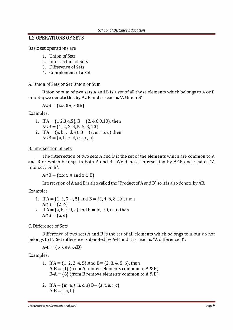
1.2 OPERATIONS OF SETSBasic set operations are1. Union of Sets2. Intersection of Sets3. Difference of Sets4. Complement of a SetA. Union of Sets or Set Union or SumUnion or sum of two sets A and B is a set of all those elements which belongs to A or Bor both; we denote this by A∪B and is read as ‘A Union B’A∪B = {x:x ∈A, x ∈B}Examples:1. If A = {1,2,3,4,5}, B = {2, 4,6,8,10}, thenA∪B = {1, 2, 3, 4, 5, 6, 8, 10}2. If A = {a, b, c, d, e}, B = {a, e, i, o, u} thenA∪B = {a, b, c, d, e, i, o, u}B. Intersection of SetsThe intersection of two sets A and B is the set of the elements which are common to Aand B or which belongs to both A and B. We denote ‘intersection by A∩B and read as “AIntersection B”.A∩B = {x:x ∈ A and x ∈ B}Intersection of A and B is also called the “Product of A and B” so it is also denote by AB.Examples1. If A = {1, 2, 3, 4, 5} and B = {2, 4, 6, 8 10}, thenA∩B = {2, 4}2. If A = {a, b, c, d, e} and B = {a, e, i, o, u} thenA∩B = {a, e}C. Difference of SetsDifference of two sets A and B is the set of all elements which belongs to A but do notbelongs to B. Set difference is denoted by A-B and it is read as “A difference B”.A-B = { x:x ∈A x∉B}Examples:1. If A = {1, 2, 3, 4, 5} And B= {2, 3, 4, 5, 6}, thenA-B = {1} (from A remove elements common to A & B)B-A = {6} (from B remove elements common to A & B)2. If A = {m, a, t, h, c, s} B= {s, t, a, i, c}A-B = {m, h}
School of Distance Education
Mathematics for Economic Analysis-I Page 10
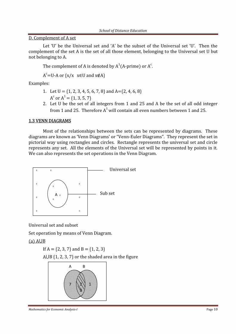
D. Complement of A setLet ‘U’ be the Universal set and ‘A’ be the subset of the Universal set ‘U’. Then thecomplement of the set A is the set of all those element, belonging to the Universal set U butnot belonging to A.The complement of A is denoted by A1(A-prime) or Ac.Ac=U-A or {x/x x∈U and x∉A}Examples:1. Let U = {1, 2, 3, 4, 5, 6, 7, 8} and A={2, 4, 6, 8}Ac or A1 = {1, 3, 5, 7}2. Let U be the set of all integers from 1 and 25 and A be the set of all odd integerfrom 1 and 25. Therefore A1 will contain all even numbers between 1 and 25.1.3 VENN DIAGRAMSMost of the relationships between the sets can be represented by diagrams. Thesediagrams are known as ‘Venn Diagrams’ or “Venn-Euler Diagrams”. They represent the set inpictorial way using rectangles and circles. Rectangle represents the universal set and circlerepresents any set. All the elements of the Universal set will be represented by points in it.We can also represents the set operations in the Venn Diagram.Universal set
Sub setUniversal set and subsetSet operation by means of Venn Diagram.(a) A⋃BIf A = {2, 3, 7} and B = {1, 2, 3}A⋃B {1, 2, 3, 7} or the shaded area in the figure
A B
7 2 13
0 0
0 0
0 0
0 0
0
A 0
0
0

School of Distance Education
Mathematics for Economic Analysis-I Page 11
(b) A⋂BIf A = {2, 3, 7} and B = {1, 2, 3} thenA⋂B = {2, 3} or shaded area in the figure
(c) Disjoint SetsIf A = {4, 5, 6} and B = {10, 11, 12} then A and B are ‘Disjoint sets” (no commonelement) They are shown as
(d) Difference of Sets (A-B)If A = {1, 2, 3, 4, 5} and B = {2, 4, 6, 8} thenA-B = {1, 3, 5} or the shaded area in the figure
(e) Complement of the set (Ac or A1)If U = {1, 2, 3, 4, 5, 6, 7, 8, 9, 10} andA = {2, 4, 6, 8, 10} then complement of A isAc = {1, 3, 5, 7, 9} or shaded area in the figure.
135
2 64 8
A B
4
5 6
10
11 12
A B
7 2 13

School of Distance Education
Mathematics for Economic Analysis-I Page 12
Important Laws of Set Operations1. Commutative Law(a) A⋃B = B⋃A(b) A⋂B = B⋂A2. Associate Law(a) A⋃(B⋃C) = (A⋃B) ⋃C(b) A⋂(B⋂C) = (A⋂B)⋂C3. Distributive Law(a) A⋃(B⋂C) = (A⋃B) ⋂ (A⋃C)(b) A⋂(B⋃C) = (A⋂B) ⋃ (A⋂C)4. De Morgan’s Law(a) (A⋃B)1 = A1⋂B1(b) (A⋂B)1 = A1⋃B1Examples:1. Using the following sets, verify that A⋃(B⋃C) = (A⋃B) ⋃CA = {1, 2, 3} B= {2, 4, 6} C= {3, 4, 5}B⋃C = {2, 3, 4, 5, 6}A⋃(B⋃C) = {1, 2, 3, 4, 5, 6}A⋃B = {1, 2, 3, 4, 5, 6}(A⋃B) ⋃C = {1, 2, 3, 4, 5, 6}∴ A⋃(B⋃C)= (A⋃B) ⋃C2. Using the following sets, verify that A⋂(B⋂C) = (A⋂B) ⋂C is A = {1, 2, 3, 4, 5, 6} ifA = {1, 2, 3, 4, 5, 6}B = {2, 4, 6} C = {3, 6, 9}B⋂C = {6} A⋂(B⋃C) = {6}(A⋂B) = {2, 4, 6}, (A⋂B) ⋂C = {6}∴ A⋂ (B⋂C)= (A⋂B) ⋂C.
1 AC 3
7
5 9
2 4A
6 810

School of Distance Education
Mathematics for Economic Analysis-I Page 13
3. Using the following sets verify that(a) A⋃(B⋂C) = (A⋃B) ⋂ (A⋃C)(b) A⋂ (B⋃C)= (A⋂B) ⋃ (A⋂C) if A = {1, 2, 3}B = {2, 3, 4} C= {3, 4, 5}(a) B⋂C = {3, 4}, A⋃(B⋂C) = {1, 2, 3, 4}A⋃B = {1, 2, 3, 4}, A⋃C = (1, 2, 3, 4, 5}(A⋃B) ⋂ (A⋃C) = {1, 2, 3, 4}(b) B⋃C = {2, 3, 4, 5}A⋂ (B⋃C)= {2, 3}A⋂B = {2, 3}, A⋂C = {3}(A⋂B) ⋃ (A⋂C) = {2, 3}∴ A⋂ (B⋃C)= (A⋂B) ⋃(A⋂C)4. If U = {0, 2, 3, 4, 5, 6, 7, 8}, A = {0, 2, 3} B={2, 4, 5} verify that (a) (A⋃B)1 = A1⋂B1 (b)(A⋂B)1 = A1⋃B1(a) A⋃B = {0, 2, 3, 4, 5}(A⋃B)1 ={6, 7, 8}A1 = {4, 5, 6, 7, 8}B1 = {0, 3, 6, 7, 8}A1⋂B1 = {6, 7, 8}∴(A⋃B)1 = A1⋂B1(b) A⋂B = {2}(A⋂B)1 = {0, 3, 4, 5, 6, 7, 8}A1 = {4, 5, 6, 7, 8}B1 = {0, 3, 6, 7, 8}A1⋃B1 = {0, 3, 4, 5, 6, 7, 8}∴(A⋂B)1 = A1⋃B1ORDERED PAIRSAn ordered pair consists of two elements say ‘a’ and ‘b’ such that one of them say ‘a’ isdesignated as the first element and the other ‘b’ is designated as the second element.An ordered pair is represented by (a, b)If (a, b) and (c, d) are two ordered pairs then, (a, b) = (c, d) if and only if a=c andb=d. Thus, the ordered pairs (a, b)≠(b, a) because a≠b and b≠a.1.4 CARTESIAN PRODUCTSLet A and B be any two non-empty sets, then the Cartesian product of these two non-empty set A and B, is the set of all possible ordered pairs (a, b) where a∈A and b∈B. Cartesianproduct is denoted by A X B (read as A cross B).A X B = {(a, b)/a∈A and b∈B}

School of Distance Education
Mathematics for Economic Analysis-I Page 14
In the Cartesian Product the first element belongs to the first set and the secondelement belongs to the second set.Examples:1. If A = {1, 2, 3} and B = {4, 5} find A X B and B X A. Are they equal?A X B = {(1, 4), (1, 5), (2, 4), (2, 5), (3, 4), (3, 5)}B X B = {(4, 1), (4, 2), (4, 3), (5, 1), (5, 2), (5, 3)}∴A X B ≠ B X A2. If A = {4, 5}, B = {1, 2} C= {3, 4} find (a) A x (B⋃C) (b) (A X B) ⋂ (A X C)(c) A X A(a) B⋃C = {1, 2, 3, 4}A X (B⋃C) = {(4, 1) (4, 2), (4, 3), (4, 4), (5, 1), (5, 2), (5, 3), (5, 4)}(b) A X B = {(4, 1), (4, 2), (5, 1), (5, 2)}A X C = {(4, 3), (4, 4), (5, 3), (5, 4)}(A X B) ⋂ (A X C) = { }(c) A X A = {(4, 4), (4, 5), (5, 4), (5, 5)}1.5 RELATIONSA relation is an association between two or more things. It may or may not be true.They are classified according to the number of elements associated(a) Binary or Dyadic RelationWhen a relation suggests a correspondence or an association between the elements oftwo sets it is called Binary or Dyadic Relation.(b) Ternary or Triadic RelationWhen a relation suggests a correspondence or an association between the elements ofthree sets it is called Ternary or Triadic relation.Most of the relations in mathematics are binary for example, Equality, Identity,equivalence greater than or less than etc.Example.1 x y1 42 83 124 16…………..…………..x 4xIn this the relation is y = 4x.
School of Distance Education
Mathematics for Economic Analysis-I Page 15
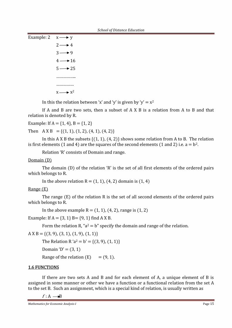
Example: 2 x y2 43 94 165 25……………..……………x x2In this the relation between ‘x’ and ‘y’ is given by ‘y’ = x2If A and B are two sets, then a subset of A X B is a relation from A to B and thatrelation is denoted by R.Example: If A = {1, 4}, B = {1, 2}Then A X B = {(1, 1), (1, 2), (4, 1), (4, 2)}In this A X B the subsets {(1, 1), (4, 2)} shows some relation from A to B. The relationis first elements (1 and 4) are the squares of the second elements (1 and 2) i.e. a = b2.Relation ‘R’ consists of Domain and range.Domain (D)The domain (D) of the relation ‘R’ is the set of all first elements of the ordered pairswhich belongs to R.In the above relation R = (1, 1), (4, 2) domain is (1, 4)Range (E)The range (E) of the relation R is the set of all second elements of the ordered pairswhich belongs to R.In the above example R = (1, 1), (4, 2), range is (1, 2)Example: If A = {3, 1} B= {9, 1} find A X B.Form the relation R, “a2 = b” specify the domain and range of the relation.A X B = {(3, 9), (3, 1), (1, 9), (1, 1)}The Relation R ‘a2 = b’ = {(3, 9), (1, 1)}Domain ‘D’ = (3, 1)Range of the relation (E) = (9, 1).1.6 FUNCTIONSIf there are two sets A and B and for each element of A, a unique element of B isassigned in some manner or other we have a function or a functional relation from the set Ato the set B. Such an assignment, which is a special kind of relation, is usually written asf : A B

School of Distance Education
Mathematics for Economic Analysis-I Page 16
or ‘f ’ is a function of A into BIt implies that if (x, y) ∈ f and (x, z) ∈ f,then y = zi.e. for each x ∈ A there is almost one y ∈ B with (x, y) ∈ f.We define a function from the set X into the set y as a set of ordered pairs (x, y) where‘x’ is an element of X and y is an element of Y such that for each x in X there is only oneordered pair (x, y) in the function P.The notation used isf : X Y or y = f (x) or x f (x)or y = f (x)A function is a mapping or transformation of ‘x’ into ‘y’ or f (x). The variable ‘x’presents elements of the ‘Domain’ and is called the independent variable. The variable ‘y’represent elements of the ‘Range’ is called the dependent variable.Domain Range
The function y = f (x) is often called a ‘single valued function’ because there is aunique ‘y’ in the range for each specified x.A function whose domain and range are sets of real number is called a real valuedfunction of a real variable.If the range consists of a single element it is called constant function. It may bewritten as y = k or f (x) = k. Where ‘k’ is constant.
x y = f (x)

School of Distance Education
Mathematics for Economic Analysis-I Page 17
CHAPTER 2FUNDAMENTAL OF LINEAR ALGEBRA-MATRICES
2.1 The Role of Linear AlgebraIn the function, Y = f(x), if both variables appear to the first power, then it can berepresented by a straight line and is known as linear function. In other words, a function ofthe form Y = + is a linear function and represented graphically by a straight line.The following are the role of linear algebra(a) It permits the expression of a complicated system of equations in a simplified form.(b) It provides a shorthand method to determine whether a solution exists before it isattempted.(c) It furnishes the means of solving the equation system.However, linear algebra can be applied only to systems of linear equations. Since manyeconomic relationships can be approximated by linear equations and other can be convertedto linear relationships, this limitation generally presents no serious problem.2.2 The Matrices : Definitions and TermsA matrix is a rectangular array of numbers, parameters or variables, each of which hasa carefully ordered place within the matrix. The numbers (parameters or variables) arereferred to as elements of the matrix and are usually enclosed in brackets. A matrix can bewritten in the following form.A =Matrices, like sets, are denoted by capital letters and the elements of the matrix areusually represented by small letters. The members in the horizondal line are called rows andmembers in the vertical line are called columns. The number of rows and the number ofcolumns in a matrix together define the dimensions or order of matrix. If a matrix contains‘m’ rows and ‘n’ columns, it is said to be diamension of m × n (read as ‘m by n’). The rownumber always precedes the column number. In that sence, the above matrix A is ofdimension 3×3. Similarly,B = 5 74 3 ×C= [9 5] ×D = 608 ×E = 0483
−20423517 ×The following are important types of matrices

School of Distance Education
Mathematics for Economic Analysis-I Page 18
(a) Square MatrixA matrix with equal number of rows and columns is called square matrix. Thus, it is a specialcase where m = n. For example4 75 2 is a square matrix of order 25 2 74 0 12 8 9 is a square matrix of order 3(b)Row vector or Row MatrixA matrix having only one row is called row vector or row matrix. A row vector will have adiamension of 1× n. For example,A = [4 8] ×B = [3 0 2] ×C = [0 4 8 1] ×(c) Column Vector or Column MatrixA matrix having only one column is called column vector or column matrix. A column vectorwill have a diamension of m × 1. For example,A = 52 ×B = 042 ×C = 4796 ×are column vectors(d) Diagonal MatrixIn a square matrix, the elements lie on the leading diagonal from left top to the rightbottom are called diagonal elements. For example in the following square matrix,A = 5 83 6The elements 5 and 6 are diagonal elements. A square matrix in which all theelements except those in the diagonal are zero is called diagonal matrix. The following areexamples of diagonal matrix.A = 8 00 5 ×B = 6 0 00 4 00 0 9 ×

School of Distance Education
Mathematics for Economic Analysis-I Page 19
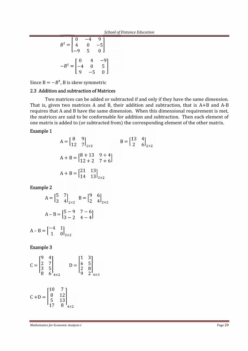
(e)Triangular MatrixIf every element above or below the leading diagonal is zero, the matrix is calledtriangular matrix. A triangular matrix may be upper triangular or lower triangular. In theupper triangular matrix, all elements below the leading diagonal are zero. The followingmatrix A is a upper triangular matrix.A = 4 7 30 8 60 0 5 ×In the lower triangular matrix, all elements above the leading diagonal are zero. Thefollowing matrix B is an example of lower triangular matrix.B = 5 0 09 3 04 8 7 ×(f) Symmetric MatrixThe matrix obtained from any given matrix A, by interchanging its rows and columnsis called its transpose and is denoted as or . If matrix A is m × n matrix, then A’ will beof n×m matrix. Any square matrix A is said to be symmetric if it is equal to its transpose.That is A is symmetric if A = . For example,A = 5 77 3 = 5 77 3Since A = , A is symmetric matrix.B = 2 3 93 6 49 4 8= 2 3 93 6 49 4 8Since B = , B is symmetric(g) Skew symmetric MatrixAny square matrix A is said to be skew symmetric if it is equal to its negativetranspose. That is, if A =− , then matrix A is skew symmetric. For example,A = 0 5−5 0= 0 −55 0− = 0 5−5 0Since A = − , A is skew symmetricB = 0 4 −9−4 0 59 −5 0
School of Distance Education
Mathematics for Economic Analysis-I Page 20
= 0 −4 94 0 −5−9 5 0− = 0 4 −9−4 0 59 −5 0Since B = − , B is skew symmetric2.3 Addition and subtraction of MatricesTwo matrices can be added or subtracted if and only if they have the same dimension.That is, given two matrices A and B, their addition and subtraction, that is A+B and A-Brequires that A and B have the same dimension. When this dimensional requirement is met,the matrices are said to be conformable for addition and subtraction. Then each element ofone matrix is added to (or subtracted from) the corresponding element of the other matrix.Example 1 A = 8 912 7 × B = 13 42 6 ×A + B = 8 + 13 9 + 412 + 2 7 + 6A + B = 21 1314 13 ×Example 2A = 5 73 4 × B = 9 62 4 ×A – B = 5 − 9 7 − 63 − 2 4 − 4A – B = −4 11 0 ×Example 3
C = 92384756 × D = 1629
3582 ×C +D = 108517
712138 ×

School of Distance Education
Mathematics for Economic Analysis-I Page 21
Example 4A = 2 2 21 1 −31 0 4 × B = 3 3 33 0 56 9 −1 × C = 4 4 45 −1 02 3 1 ×A + B – C = 1 1 1−1 2 25 6 2 ×2.4 Scalar MultiplicationIn the matrix algebra, a simple number such as 1,2, -2, -1 or 0.5 is called a scalar.Multiplication of a matrix by a scalar or a number involves multiplication of every element ofthe matrix by the number. The process is called scalar multiplication.Let ‘A’ by any matrix and ‘K’ any scalar, then the matrix obtained by multiplying everyelement of A by K and is said to be scalar multiple of A by K because it scales the matrix up ordown according to the size of the scalar.Example 1K = 8 and A = 6 92 78 4KA = 8 6 92 78 4KA = 8 × 6 8 × 98 × 2 8 × 78 × 8 8 × 4KA = 48 7216 5664 32Example 2
K = 7 and A = 2 2 22 1 −31 0 4KA = 14 14 1414 7 −217 0 28Example 3A = 6 7 43 −1 02 4 5 and K = 5

School of Distance Education
Mathematics for Economic Analysis-I Page 22
KA = 5 6 7 43 −1 02 4 5KA = 30 35 2015 −5 010 20 25Example 4K = -2 and A = 3 −42 −9KA = -2 3 −42 −9KA = −6 8−4 182.5 Vector MultiplicationMultiplication of a row vector ‘A’ by a column vector B requires that each vector haveprecisely the same number of elements. The product is then found by multiplying theindividual elements of the row vector by their corresponding elements in the column vectorand summing the products. For example, ifA = [ ] ×andB = ×AB = (ad) + (bc) + (cf)Thus, the product of row-column multiplication will be a single number or scalar.Row-column vector multiplication is very important because it serves the basis for all matrixmultiplications.Example 1A = [4 2] × B = 35 ×AB = [(4 × 3) + (2 × 5)]AB = 22Example 2A = [5 1 3] × B = 263 ×AB = [(5 × 2) + (1 × 6) + (3 × 3)]AB = 25

School of Distance Education
Mathematics for Economic Analysis-I Page 23
Example 3A = [12 −5 6 11] × B = 32−86AB = [(12 × 3) + (−5 × 2) + (6 × −8) + (11 × 6)]AB = 44Example 4A = [9 6 2 0 −5] × B = ⎣⎢⎢⎢
⎡ 213581 ⎦⎥⎥⎥⎤
AB = [(9 × 3) + (6 × 13) + (2 × 5) + (0 × 8) + (−5 × 1)]AB = 1012.6 Multiplication of MatricesThe matrices A and B are said to be conformable for multiplication if and only if thenumber of columns in the matrix A is equal to the number of rows in matrix B. That is, tofind the product AB, conformity condition for multiplication requires that the columndimension of A (the lead matrix in the expression AB) must be equal to the row dimension ofB (the lag matrix).In general, if A is of order m × n, then B should be of the order n×p and dimension ofAB will be m×p. That is, if dimension of A is 1×2 and dimension of B is 2×3, then AB will beof 1×3 dimension. The procedure of multiplication is that take each row and multiply it witheac column. The row-column products, called ‘inner products’ are then used as elements inthe formation of the product matrix.Example 1A = 6 125 1013 2 × B = 1 7 82 4 3 ×Since matrix A is of 3×2 dimension and B is of 2×3 diamension, the matrices areconformable for multiplication and the product AB will be of 3×3 dimension.AB = 6 × 1 + 12 × 2 6 × 7 + 12 × 4 6 × 8 + 12 × 35 × 1 + 10 × 2 5 × 7 + 10 × 4 5 × 8 + 10 × 313 × 1 + 2 × 2 13 × 7 + 2 × 4 13 × 8 + 2 × 3AB = 30 90 8425 75 7017 99 110 ×Example 2A = 12 1420 5 × B = 3 90 2 ×

School of Distance Education
Mathematics for Economic Analysis-I Page 24
AB = 12 × 3 + 14 × 0 12 × 9 + 14 × 220 × 3 + 5 × 0 20 × 9 + 5 × 2AB = 36 13660 190 ×Example 3 A = 4 79 1 × B = 3 8 52 6 7 ×AB = 4 × 3 + 7 × 2 4 × 8 + 7 × 6 4 × 5 + 7 × 79 × 3 + 1 × 2 9 × 8 + 1 × 6 9 × 5 + 1 × 7AB = 26 74 6929 78 52 ×Example 4If A = 6 19 4 compute= A × A = 6 19 4 6 19 4= 6 × 6 + 1 × 9 6 × 1 + 1 × 49 × 6 + 4 × 9 9 × 1 + 4 × 4= 45 1090 252.7 Commutative, Associative and Distributive Laws in AlgebraIn ordinary algebra, the additive, subtractive and multiplicative operations obeycommutative, associative and distributive laws. Most, but not all, of these laws also apply tomatrix operations.(a) Matrix Addition and SubtractionMatrix addition and subtraction is commutative.Commutative law of addition states that A + B = B+ACommutative law of subtraction states that A –B = -B + AAssociative law of addition states that (A+B)+C = A +(B+C)Associative law of subtraction states that (A +B)-C = A +(B-C)(b)Matrix MultiplicationMatrix multiplication, with few exception is not commutative. That is AB≠BA. Oneexception is a case when A is a square matrix and B is on identity matrix. At the sametime,scalar multiplication is commutative. That is KA =AK, where K is a scalar. But matrixmultiplication is a associative. That (AB)C = A(BC). If matrices are conformable, the matrixmultiplication is also distributive. Distributive law states that A(B+C) = AB +AC.Example 1Given A = 3 10 2 and B = 6 23 4 prove that matrix addition and subtraction is commutative.

School of Distance Education
Mathematics for Economic Analysis-I Page 25
Commutative law of addition states that A+B = B + AA + B = 9 33 6B + A = 9 33 6A + B = B + A ∴ matrix subtraction is commutativeExample 2Given A = 6 2 79 5 3 B = 9 1 34 2 6 C = 7 5 110 3 8 prove that matrix addition satisfyassociative law.Associative law of addition (A+B)+C = A + (B+C)A+B = 15 3 1013 7 9(A+B)+C = 22 8 1123 10 17B + C = 16 6 414 5 14A + (B +C) = 22 8 1123 10 17(A+B) +C = A + (B+C) ∴ matrix addition satisfy associative lawExample 3Given A = 1 23 4 B = 0 −16 7 prove that AB ≠ BAAB = 12 1324 25BA = −3 −427 40∴ AB ≠ BAExample 4Given A = [7 1 5] B = 6 52 43 8 C = 9 43 10Prove that matrix multiplication is associative.Associative law of multiplication (AB)C = A(BC)AB = [59 79](AB)C = [768 1026]BC = 69 7430 4851 92A(BC) = [768 1026](AB)C = A(BC) ∴ matrix multiplication is associative.

School of Distance Education
Mathematics for Economic Analysis-I Page 26
2.8 Identity and Null MatricesA diagonal matrix in which each of the diagonal element is unity is said to be aidentity or unit matrix and is denoted by I. when a subscript is used, as , n denotes thedimension of the matrix (n × n). The identity matrix is similar to the number 1 in algebrasince multiplication of a matrix by an identity matrix leaves the original matrix unchanged.That is, AI = IA=A. Multiplication of an identity matrix by itself leaves the identity matrixunchanged. That is , I × I= = I. The identity matrix is symmetric and idempotent.Following are examples of identity matrix.I = 1 00 1 ×I = 1 0 00 1 00 0 1 ×On the other hand, a matrix in which every element is zero is called null matrix orzero matrix. Null matrix can be of any dimension. It is not necessarily square. Addition orsubtraction of the null matrix leaves the original matrix unchanged. Multiplication by a nullmatrix produces a null matrix. Following are examples of null matrix.0 0 00 0 0 × 0 00 00 0 ×0 00 0 ×
2.9 Matrix Expression of a system of Linear EquationsMatrix algebra permits concise expression of a system of linear equation. Given thefollowing system of linear equations.+ =+ =can be expressed in the matrix form asAx=Bwhere,A = ×X = ×B = ×Here ‘A’ is the coefficient matrix, ‘x’ is the solution vector and B is the vector ofconstant terms. X and B will always be column vectors. Since A is 2 × 2 matrix and X is 2 × 1vector, they are conformable for multiplication and the product matrix will be 2 × 1.

School of Distance Education
Mathematics for Economic Analysis-I Page 27
Example 1Given, 7 + 3 = 454 + 5 = 29In matrix form AX = B7 34 5 × × = 4529 ×Example 2Given, 7 + 8 = 1206 + 9 = 92In matrix form AX = B7 86 9 × × = 12092 ×Example 3Given, 2 + 4 + 9 = 1432 + 8 + 7 = 2045 + 6 + 3 = 168In matrix form AX = B2 4 92 8 75 6 3 × × = 143204168 ×Example 4Given, 8w + 12x – 7y + 2z = 1393w – 13x + 4y + 9z = 242In matrix form AX = B8 12 −7 23 −13 4 9 × × = 139242 ×2.10 Row OperationsRow operations involve the application of simple algebraic operations to the rows of amatrix. With no change in the linear relationship, we have three basic row operations. Theyare

School of Distance Education
Mathematics for Economic Analysis-I Page 28
1. Any two rows of a matrix to be interchanged.2. Any row or rows to be multiplied by a constant provided the constant does not equalto zero.3. Any multiple of a row to be added to or subtracted from any other row.For example, given 5x + 2y = 168x + 4y = 28Without any change in the linear relationship, we may(1) Interchange the two rows8x + 4y = 285x + 2y = 16(2) Multiply any row by a constant, say first row by2x + y = 75x + 2y = 16(3) Subtract 2 times of first row from the second row, that is2[(2 + ) = 7] ⇒ 4x + 2y = 145x + 2y = 16 -14x + 2y = 14--------------------x = 2
REFERENCE(1) Edward .T. Dowling : “ Introduction to Mathematical Economics”Second Edition . Schaum’s outline series(2) Alpha C. chiang: Fundamental Methods of Mathematical Economics,MC Graw Hill(3) Manmohan Gupta : Mathematics for Business and Economics

School of Distance Education
Mathematics for Economic Analysis-I Page 29
CHAPTER 3MATRIX INVERSION3.1 Determinants and NonsingularityThe determinant is a single number or scalar associated with a square matrix.Determinants are defined only for square matrix. In other words, the determinant of asquare matrix A denoted as |A| is a uniquely defined number or scalar associated with thatmatrix.It the determinant of a square matrix is equal to zero, the determinant is said tovanish and the matrix is termed as “singular”. That is, a singular matrix is the one in whichthere exists a linear relationship or dependence between atleast two rows or columns. If |A|≠ 0, matrix A is called “nonsingular” and all its rows and columns are linearly independent.3.2 DeterminantsIf A = [ ] is a 1 1 matrix, then the determinant of A, that is |A| is a11 itself. If A is 2 2matrix, likeThen |A| is derived by taking the product of the two elements on the principal diagonal andsubtracting form it the product of the elements off principal diagonal. That is,|A| = ( )- ( )Thus, |A| is obtained by cross multiplication of the elements. The determinant of a 22 square matrix is called second order determinant.The determinant of order three is associated w ith a 3 3 matrix. Given.A =Then |A| = - +|A| = a Scalar
Thus, the third order determinant is the summation of three products. To derive thethree products;1. Take the first element of the first row, that is, by the determinant of the remainingelement.2. Take the second element of the first row, ie, and mentally delete the row andcolumn in which it appears. Then multiply by -1 times the determinant of theremaining element.3. Take the third element of first row, ie, and mentally delete the row and column inwhich it appears. Then multiply by the determinant of the remaining element.

School of Distance Education
Mathematics for Economic Analysis-I Page 30
In the like manner, determinant of a 4 4 matrix is the sum of four products. Thedeterminant of a 5 5 matrix is the sum five products and so on.Example 1 A = 2 33 6|A| = (2 6) – (3 3)|A| = 3Example 2 B = 2 1−3 2|B| = (2 2) – (-3 1)|B| = 7Example 3 C = −3 6 21 5 44 −8 2|C| = −3 5 4−8 2 -6 1 44 2 + 2 1 54 −8|C| = -98Example 4D = 1 3 20 2 −14 1 5|D| = 1 2 −11 5 -3 0 −14 5 + 2 0 24 1|C| = -173.3 Properties of a DeterminantThe following are important proportion of a determinant.(1) The value of the determinant does not change, if the rows and columns of it areinterchanged. That is, the determinant of a matrix equals the determinant of itstranspose. Thus, |A| = |A |If A = 6 47 9|A| = (6 9) – (4 7) = 26|A | = 6 47 9|A | = (6 9) – (4 7) = 26∴ | A| = |A |=======

School of Distance Education
Mathematics for Economic Analysis-I Page 31
(2) The inter change of any two rows or any two columns will alter the sign, but not thenumerical value of the determinant.A = 3 1 07 5 21 0 3 = |A| = 26Now interchanging first and third column, forming BB = 0 1 32 5 73 0 1 = |B| = -26 = - |A|
(3) If any two rows or columns of a matrix are identical or proportional, that is, lineallydependent, the determinant is zero.If A = 2 3 14 1 02 3 1 = |A| = 0, Since first and third row are identical.(4) The multiplication of any one row or one column by a scalar or constant, say ‘K’ willchange the value of the determinant K fold. That is, multiplying a single row orcolumn of a matrix by a scalar will cause the value of the determinant to bemultiplied by the scalar.If A = 3 5 72 1 44 2 3 = |A| = 35
Now, forming a new matrix B, by multiplying the first row of a by scalar 2, we haveB = 6 10 142 1 44 2 3 |B| = 70 , that is 2 |A|
(5) The determinant of a triangular matrix is equal to the product of the elements onprincipal diagonal. For the following lower triangular matrix, A, whereA = −3 0 02 −5 06 2 3 |A| = 60 , that is -3 -5 4(6) If all the elements of any row or column are zero then determinant is also zero.
If A = 3 8 49 2 10 0 0 |A| = 0, Since all the elements of third row is zero.(7) Addition or subtraction of a non-zero multiple of any one row or column from anotherrow or column does not change the value of determinant.If A = 20 310 2 = |A| = 10Subtracting two times of column two from column one and forming a new matrix B,B = 14 36 2 |B| = 10

School of Distance Education
Mathematics for Economic Analysis-I Page 32
(8) If every element in a row or column of a matrix is the sum of two numbers, then thegiven determinant can be expressed as sum of two determinant.A = 2 + 3 14 + 1 5 |A| = 20That is, A = 2 14 5 + A = 3 11 5 = |A | = 6|A | = 14|A | + |A | = 20 which is |A| itself3.4 Minors and cofactorsEvery element of a square matrix has a minor. It is the value of determinant formedwith elements obtained when the row and the column in which the element lies are deleted.Thus, a minor Mij is the determinant of the sub matrix formed by deleting the ith row and jthcolumn of the matrix.For example, if A =Minor of Minor of Minor ofSimilarly
Since all the minors have two rows and columns, it is also called minor of order K = 2or second order minor of determinant of A.A cofactor (Cij) is a minor with a prescribed sign. Cofactor of an element is obtainedby multiplying the minor of the element with (-1)i + j , where ‘i’ is the number of row and j isthe number of column.That is Cij = (-1)i + j MijIn the previous matrix ACofactor of ( ) ( ) and so on.Cofactor matrix is a matrix in which every element of Cij is replaced with its cofactorsCij.

School of Distance Education
Mathematics for Economic Analysis-I Page 33
Example 1If A = 6 712 9Cofactor of 6 = (−1) 9“ 7 = (−1) 12“ 12 = (−1) 7“ 9 = (−1) 6∴ Cij = 9 −12−7 6Example2B = −2 −14 6Cofactor of -2 = (−1) 6“ -1= (−1) 4“ 4= (−1) -1“ 6= (−1) -2∴ Cij = 6 −41 −2Example 3A = 6 2 75 4 93 3 1Matrix of cofactors Cij = −23 22 319 −15 −12−10 −19 14Example 4A = 2 3 14 1 25 3 4Matrix of cofactors Cij = −2 −6 7−9 3 95 0 −103.5 Cofactor and Adjoint MatrixAn adjoint matrix is the transpose of cofactor matrix. That is adjoint of a given squarematrix is the transpose of the matrix formed by cofactors of the elements of a given squarematrix, taken in order. In other words, adjoint ofA = [Cij]

School of Distance Education
Mathematics for Economic Analysis-I Page 34
Example 1 A = 7 124 3Matrix of cofactors Cij = 3 −4−12 7Adj A = [Cij] = 3 −12−4 7Example 2 A = 9 −16−20 7Matrix of cofactors Cij = 7 2016 9Adj A = [Cij] = 7 1620 9Example 3 A = 1 1 11 2 −32 −1 3Matrix of cofactors Cij = 3 −9 −5−4 1 3−5 4 1Adj A = [Cij] = 3 −4 −5−9 1 4−5 3 1Example 4A = 13 −2 8−9 6 −4−3 2 −1Matrix of cofactors Cij = 2 3 014 11 −20−40 −20 60Adj A = [Cij] = 2 14 −403 11 −200 −20 603.6 Inverse MatricesFor a square matrix A, if there exist another square matrix B such thatAB = BA = I, then B is said to be inverse matrix of A and is denoted as A-1.That is, AA-1 = A-1A = IMultiplying a matrix by its inverse reduces it to an identity matrix. For a given matrixA, there exist inverse only if (1) A is a square matrix.(2) A is non singular |A| ≠ 0

School of Distance Education
Mathematics for Economic Analysis-I Page 35
Again, if B is the inverse of A, then A is inverse of B. The formula for deriving theinverse is A = .| |Example 1 A = 24 158 7|A| = (24 7) – (8 15) = 48Matrix of cofactors Cij = 7 −8−15 24Adj . A = [Cij] = 7 −15−8 24A = .| | =A =
Example 2 A = −7 16−9 13|A| = 53Matrix of cofactors Cij = 13 9−16 −7Adj. A = CijT = 13 −169 −7A = .| | =A =
Example 3A = 0 1 11 2 03 −1 4|A| = -11
Matrix of cofactors Cij = 8 −4 −7−5 −3 3−2 1 −1

School of Distance Education
Mathematics for Economic Analysis-I Page 36
Adj. A = CijT = 8 −5 −2−4 −3 1−7 3 −1A = .| | = ⎣⎢⎢⎢
⎡⎦⎥⎥⎥⎤
Example 4A = 14 0 69 5 00 11 8|A| = 1154
Matrix of cofactors Cij = 40 −72 9966 112 −154−30 54 70Adj. A = CijT = 40 66 −30−72 112 54−99 −154 70A = .| | = ⎣⎢⎢⎢
⎡⎦⎥⎥⎥⎤
3.7 Solving linear Equations with the InverseAn inverse matrix can be used to solve linear equations. Consider the following set ofequations + =+ =Now settingA = X = B =In matrix form, the system of equation isAX = BIn matrix A is nonsingular so that A-1 exist, then multiplication of both sides by A-1A-1AX = A-1BIX = A-1 BX = A-1 B

School of Distance Education
Mathematics for Economic Analysis-I Page 37
This gives the solution of above equation. Thus, the solving of equation is given bythe product of inverse matrix of the coefficient matrix (A-1) and the column vector ofconstants B.Example 1 4 + 3 = 282 + 5 = 42In matrix form AX = B4 32 5 = 2842X = A-1BX = A-1 BA = .| ||A| = (4 5) – (2 3) = 14Matrix of cofactors Cij = 5 −2−3 4Adj. A = CijT = 5 −3−2 4A = .| | =X = A-1 B = 2842X = 18∴ x1 = 1 x2 = 8Example 2 6 + 7 = 562 + 3 = 44AX = B6 72 3 = 5644X = A-1BA = .| |
School of Distance Education
Mathematics for Economic Analysis-I Page 38
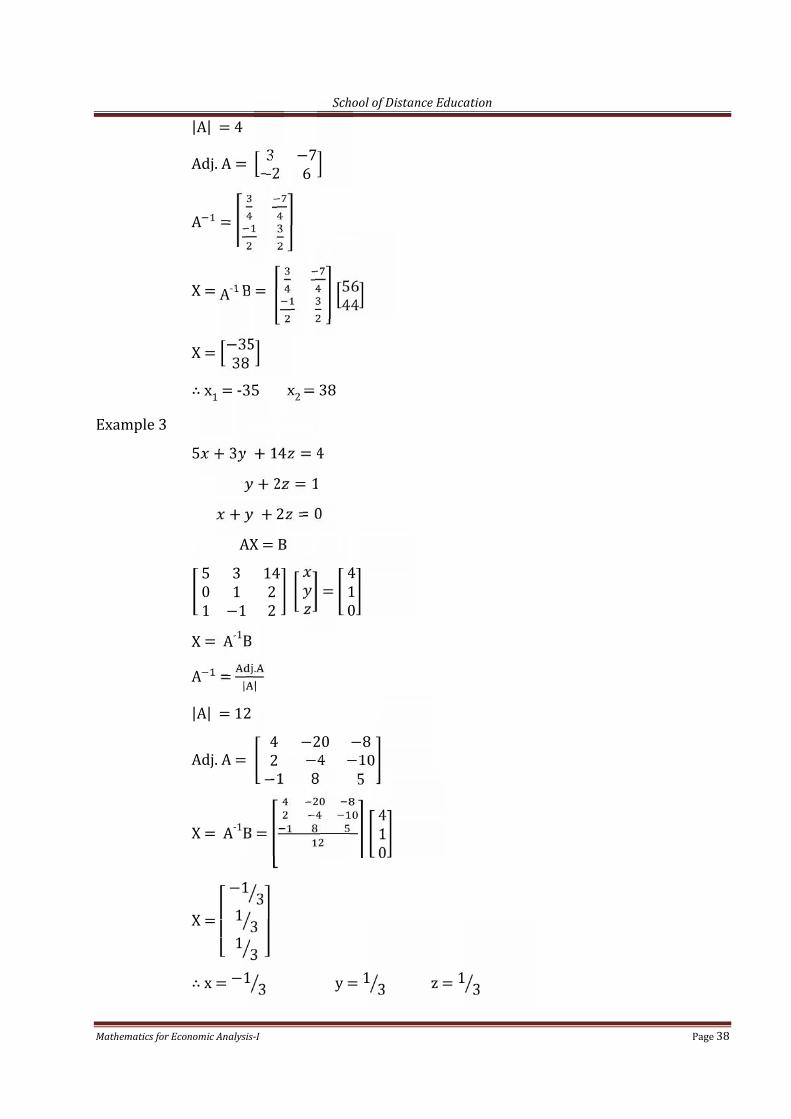
|A| = 4Adj. A = 3 −7−2 6A =X = A-1 B = 5644X = −3538∴ x1 = -35 x2 = 38Example 3 5 + 3 + 14 = 4+ 2 = 1+ + 2 = 0AX = B5 3 140 1 21 −1 2 = 410X = A-1BA = .| ||A| = 12Adj. A = 4 −20 −82 −4 −10−1 8 5X = A-1B = 410X = ⎣⎢⎢
⎡ −1 31 31 3 ⎦⎥⎥⎤
∴ x = −1 3 y = 1 3 z = 1 3
School of Distance Education
Mathematics for Economic Analysis-I Page 39
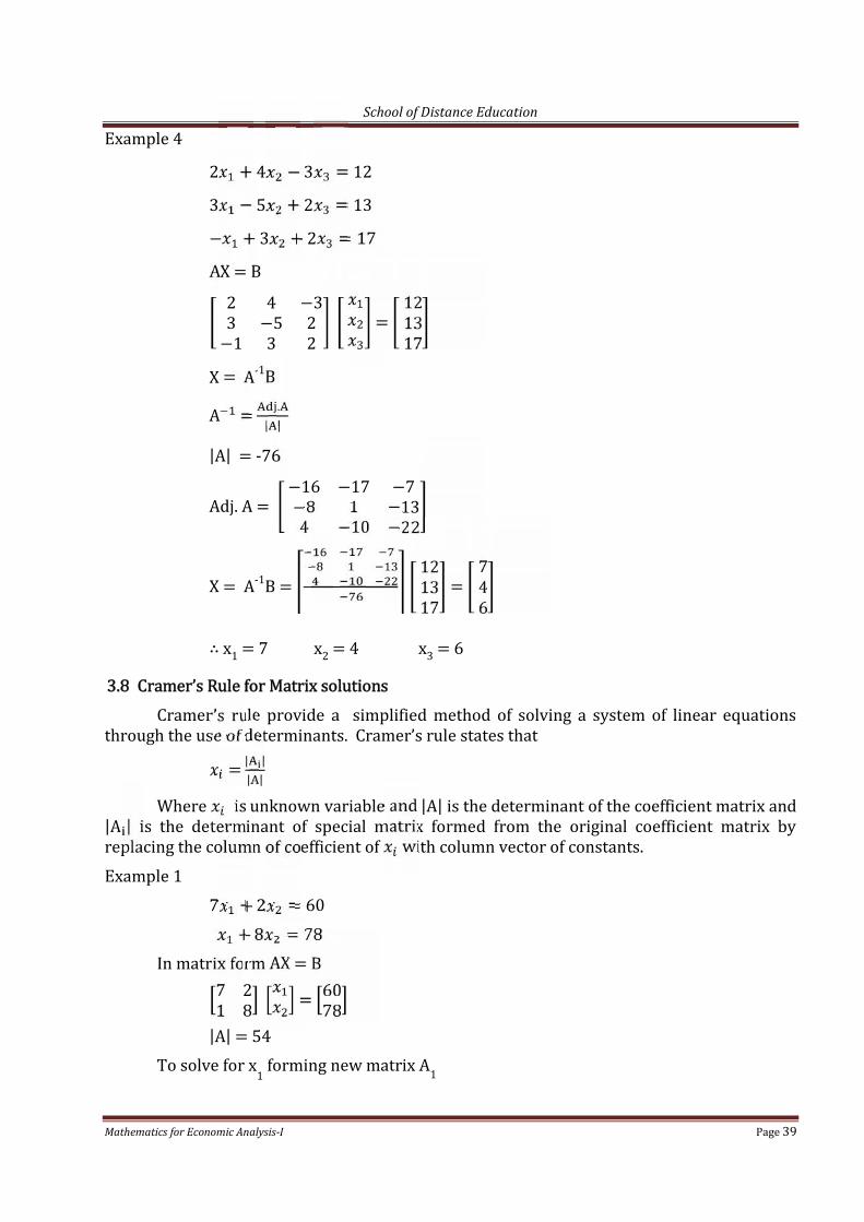
Example 4 2 + 4 − 3 = 123 − 5 + 2 = 13− + 3 + 2 = 17AX = B2 4 −33 −5 2−1 3 2 = 121317X = A-1BA = .| ||A| = -76Adj. A = −16 −17 −7−8 1 −134 −10 −22X = A-1B = 121317 = 746∴ x1 = 7 x2 = 4 x3 = 63.8 Cramer’s Rule for Matrix solutionsCramer’s rule provide a simplified method of solving a system of linear equationsthrough the use of determinants. Cramer’s rule states that= | || |Where is unknown variable and |A| is the determinant of the coefficient matrix and|A | is the determinant of special matrix formed from the original coefficient matrix byreplacing the column of coefficient of with column vector of constants.Example 1 7 + 2 = 60+ 8 = 78In matrix form AX = B7 21 8 = 6078|A| = 54To solve for x1 forming new matrix A1
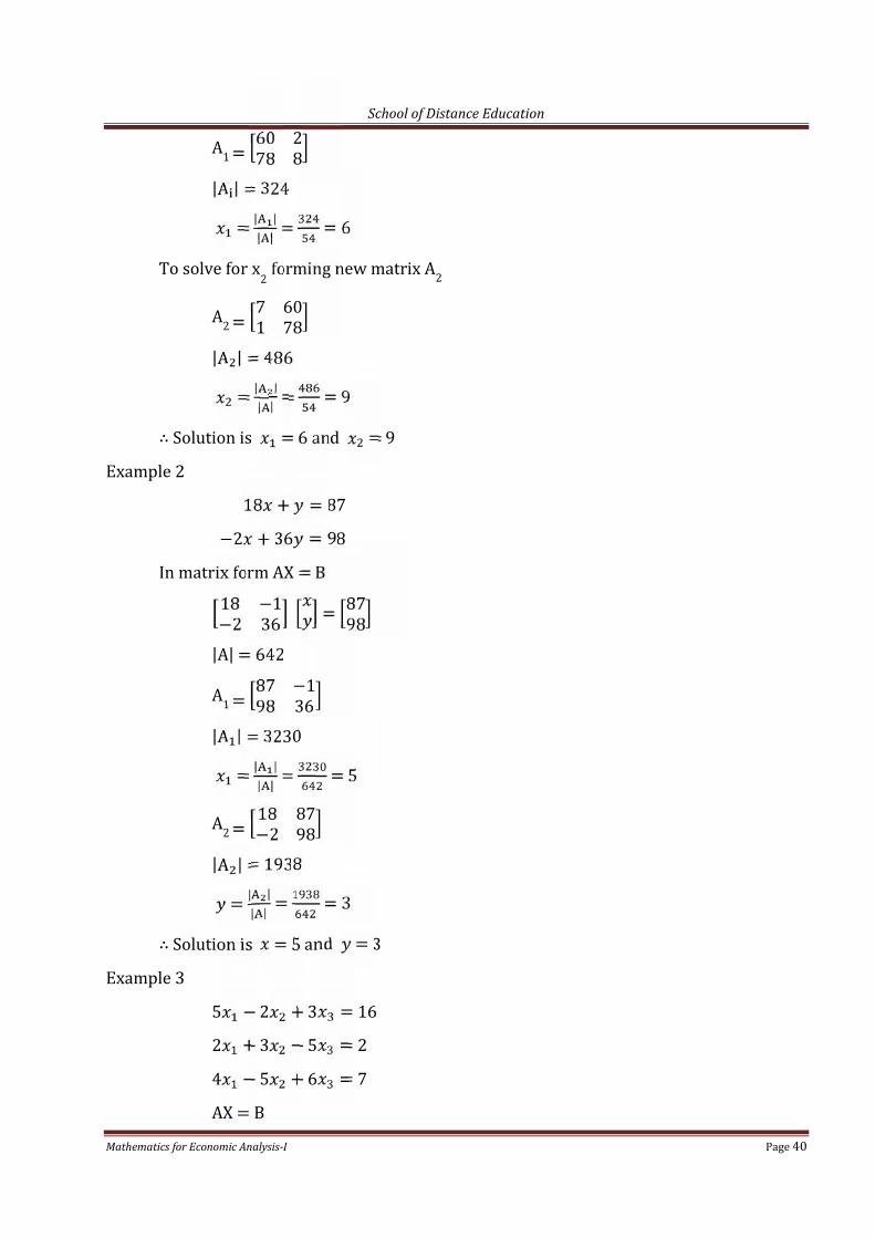
School of Distance Education
Mathematics for Economic Analysis-I Page 40
A1 = 60 278 8|A | = 324= | || | = = 6To solve for x2 forming new matrix A2A2 = 7 601 78|A | = 486= | || | = = 9∴ Solution is = 6 and = 9Example 2 18 + = 87−2 + 36 = 98In matrix form AX = B18 −1−2 36 = 8798|A| = 642A1 = 87 −198 36|A | = 3230= | || | = = 5A2 = 18 87−2 98|A | = 1938= | || | = = 3∴ Solution is = 5 and = 3Example 3 5 − 2 + 3 = 162 + 3 − 5 = 24 − 5 + 6 = 7AX = B

School of Distance Education
Mathematics for Economic Analysis-I Page 41
5 −2 32 3 −54 −5 6 = 1627|A| = -37A1 = 16 −2 32 3 −57 −5 6|A | = -111= | || | = = 3A2 = 5 16 32 2 −54 7 6|A | = -259x2 = | || | = = 3A3 = 5 −2 162 3 24 −5 7|A | = -185X3 = | || | = = 5∴ Solution is = 3, = 7 and = 5Example 4 11p − p − p = 31−p + 6p − 2p = 26−p − 2p + 7p = 24AX = B11 −1 −1−1 6 −2−1 −2 7 ppp = 312624|A| = 401A1 = 31 −1 −126 6 −224 −2 7|A | = 1604p = | || | = = 4

School of Distance Education
Mathematics for Economic Analysis-I Page 42
A2 = 11 31 −1−1 26 −2−1 24 7|A | = 2807p2 = | || | = = 7A3 = 11 −1 31−1 6 26−1 −2 24|A | = 2406p3 = | || | = = 6∴ Solution is p = 4, p = 7 and p = 63.9 Rank of a matrixThe rank of matrix of A, denoted as P(A) is defined as the maximum number oflinearly independent rows or columns. If square matrix A is non singular, such that |A| ≠ 0,then rank of A will be the order of the matrix itself and rows and columns are linearlyindependent.Example 1 A = 2 33 6|A| = 3Since A is non singular P(A) = 2Example 2 B = 4 28 4|B| = 0B is singular and hence P(B) = 1Example 3 C = −3 6 21 5 44 −8 2|C| = -98C is non singular P(C) = 3Example 4 D = 1 2 33 6 92 4 6|D| = 0

School of Distance Education
Mathematics for Economic Analysis-I Page 43
Since D = 0, D is singular and P(D) ≠ 3. Now trying various 2 2 sub matrices,starting from upper left corner.1 23 6 = 6 - 6 = 02 36 9 = 18 - 18 = 03 62 4 = 12 - 12 = 06 94 6 = 36 - 36 = 0With all the determinants of different 2 2 submatrices are equal to zero, non of twoor columns are independent. Hence P(D) ≠ 2 and P (D) = 1.Reference:(1) Edward R Dowling : Introduction to Mathematical Economics SecondEdition, Schaum’s outline series.(2) Alpha C Chiang : Fundamental Methods of Mathematical Economics,MC Graw Hill.(3) G.S. Monga : Mathematics and Statics for Economics VikadPublishing House Pvt. Ltd.

School of Distance Education
Mathematics for Economic Analysis-I Page 44
CHAPTER IVBASIC MATHEMATICAL CONCEPTS4. 1: EXPONENTSIn the expression an the base is ‘a’ and ‘n’ is the power or the exponent or the index.The value is obtained by multiplying ‘a’ by itself ‘n’ times. The expression an is calledexponential expression. The theory that deals with the expressions of the type an is calledtheory of indices.Some Basic Concepts1. Positive Integral PowerIf n is a positive integer, an is defined as the product of n factors each of which is ‘a’i.e., an = a x a x a ………………….. (n factors)Eg: 25 = 2 x 2 x 2 x 2 x 2 = 3253 = 5 x 5 x 5 = 1252. Zero Power (Zero Exponent)Any number other than zero raised to zero = 1i.e. a0 = 1 if a ≠ 0Eg: (1) 50 = 1(2) ( ½)0 = 13. Negative Integral PowerIf n is a positive integer, then a-n = , where a ≠ 0Eg: (1) 2-4 = =(2) 5-2 = =Here a-n is the reciprocal of an.4. Root of the Number(a) Square rootSquare root of a number ‘a’ is another number ‘b’ whose square is ‘a’.If a2 = b, then ‘a’ is the square root of ‘b’i.e. a= √ or a = b½Eg: If 102 = 100 then 10 = √100 or 100½(b) nth Root ofIf an = b, then ‘a’ is the nth root of ‘b’ and it is written as √ or b1/nEg: 34 = 81 then 3 = √81 = 81¼

School of Distance Education
Mathematics for Economic Analysis-I Page 45
5. Positive Fractional PowerIf ‘m’ and ‘n’ are positive integers, then is defined as the nth root of mthpower of a.= √ mEg: (1) (32) = √32 3 = 23 = 8(2) (−64) = √−64 4 = -44 = 2566. Negative Factional PowerIf ‘m’ and ‘n’ are positive integers, then is defined asEg: (1) (32) = ( ) = √ = =(2) (−64) = ( ) = √ = =
Laws of Indices (Rules of Exponent)1. am . an = am+n2. = am-n3. ( ) = amn4. ( )n = xn . yn5. n =6. =Examples1. Find the values of (a) 100 (b) 5-3 (c) 125 (d) (−8)(a) 100 = 1(b) 5 = =(c) 125 = √125 = 5(d) (−8) = √−8 2 = (-2)2 = 42. Simplify the following(a) (0.0001) (b) 9 . 243 . 729(c) [(−8)2]2 ÷ (-4)4 (d) xa-b. xb-c . xc-a

School of Distance Education
Mathematics for Economic Analysis-I Page 46
(a) (0.0001) = 0.1 x 0.1 x 0.1 x 0.1 = (0.1)4(0.0001) = [(0.1)4]1/4 = 0.1 = 0.1=====(b) 9 . 243 . 729 = √9 3 x √243 4 x √729 5= 33 x 34 x 35 = 3 3+4+5 = 312= 531441=======(c) [(−8)2]2 ÷ (-4)4(-8)2 = [(−23)2]2 = (−23)4 = (−2)12 = (−22)6 = (22)6 = 46[(−8)2]2 ÷ (-4)4 = = 4 = 42 = 16=======(d) xa-b. xb-c . xc-a = xa-b+b-c+c-a = x0 = 1======4.2 POLYNOMIALSIn the expression such as 10x2, x is called the variable because it can assume anynumber of different values, and 10 is reffered to as the coefficient of ‘x’.The expressions consisting simply of a real number or a coefficient times one or morevariables raised to the power of a positive integer one called monomials. A monomial canalso be a variable, like ‘x’ or ‘y’. It can also be a combination of these.Ex: (1) 4x5 (2) 3y2 (3) 10xyzA polynomial is an algebraic expression with a finite number of terms. Monomials canbe added or subtracted to form polynomials. Each of the monomials comprising apolynomial is called a term. Terms that have the same variables and exponents are calledlike terms. Like terms in polynomials can be added or subtracted by adding theircoefficients. Unlike items cannot be so added or subtracted.Ex: (1) 10x2 + 4x2 = 14x2(2) 25xy + 5xy – 20xy = 10xy(3) (6x5 + 5x4 – 10x) + (4x5 + 3x4 + 8x) = 10x5 + 8x4 – 2x(4) (2x2 + 4y) + (4x2 + 3z) = 6x2 + 4y + 3zLike and unlike terms can be multiplied or divided by multiplying or dividing both thecoefficient and variables.Ex: (1) (5x) (10y2) = 50xy2(2) (5x2y3) (6x4y2) = 30x6y5(3) = 5x2yz
School of Distance Education
Mathematics for Economic Analysis-I Page 47
Multiplication of two polynomialsIn multiplying two polynomials, each term in the first polynomial must be multipliedby each term in the second and their product is added.Ex: (1) (5x + 6y) (4x + 2y)= (5x)(4x) + (5x)(2y) + (6y)(4x) + (6y)(2y)= 20x2 + 10xy + 24xy + 12y2= 20x2 + 34xy + 12y2====================(2) (6x – 4y) (3x – 5y)= (6x)(3x) + (6x)(-5y) – (4y)(3x) – (4y)(-5y)= 18x2 – 30xy – 12xy + 20y2= 18x2 – 42xy + 20y2===================Problems (1) (2x + 3y)(8x – 5y -7z) [Ans: 16x2 + 14xy – 14xz – 21yz – 15y2](2) (x + y) (x – y) [Ans: x2 – y2]4.3 FACTORINGFactoring polynomial expressions is not quite the same as factoring numbers. But theconcept of factoring is very similar in both cases. When factoring numbers or polynomials,we are finding numbers or polynomials that divide out evently from the original numbers orpolynomials. But in the case of polynomials, we are dividing numbers and variables out ofexpressions, not just dividing number out of numbers.Ex: 2x + 6 = 2(x) + 2(3) = 2(x + 3)Factoring means “dividing out and putting in front of the parentheses”. (Here nothing“disappears” when we factor, but the things are merely rearranged.)Ex: Factor 4x + 12In the above example the only thing common between the two terms (i.e. the onlything that can be divided out of each term and then moved up front) is ‘4’.Therefore 4x + 12 = 4 ( )When we divide the ‘4’ out of the 4x, we get ‘x’. So we have to put that ‘x’ as the firstterm inside the parentheses.i.e. 4x + 12 = 3 (x )When we divide the ‘4’ out of the +12 we get ‘4’. So we have to put it as the secondterm inside the parentheses.4x + 12 = 3(x + 4)

School of Distance Education
Mathematics for Economic Analysis-I Page 48
Ex: (2) Factor 5x – 35Ans: 5(x – 7)(3) Factor 8x2 – 5xAns: x(8x – 5)(4) Factor x2y3 + xyAns: xy(xy2 + 1)(5) Factor 3x3 + 6x2 – 15xAns: Here ‘3’ and ‘x’ are common. So we can factor a ‘3’ and ‘x’out of each term.3x3 = 3x(x2)6x2 = 3x(2x)-15x = 3x (-5)3x3 + 6x2 – 15x = 3x(x2 + 2x -5)(6) 2(x-y) – b(x – y)Ans: (x – y)(2 – b)(7) Factor x(x-2) + 3(2 – x)Ans: (x – 2)(x – 3)(8) Factor xy – 5y – 2x + 10Here there is no common factor in all four terms. So, we have to factor “in pairs”. Forthis split this expression into two pairs of terms and then factor the pairs separately.xy – 5y – 2x + 10 = y(x – 5) – 2x + 10 = y(x – 5) – 2(x – 5)Here (x - 5) is common.(x – 5)(y – 2)(9) Factor x2 + 4x – x – 4Ans: x(x + 4) – 1(x + 4)Here (x + 4) is common(x + 4)(x – 1)===========(10) x2 – 5x – 6Ans: Here to get two pairs we have to split up the expression‘-5x’ into -6x+1x then the function will become.x2 – 6x + 1x – 6 = x (x – 6) + 1 (x – 6)]= (x – 6) (x + 1)===========(11) Factor 6x2 – 13x + 6Ans: 6x2 – 9x – 4x + 6 = 3x(2x – 3) – 2(2x – 3)= (2x – 3)(3x – 2)============

School of Distance Education
Mathematics for Economic Analysis-I Page 49
4.4 EQUATIONS : LINEAR AND QUADRATICA mathematical statement setting two algebraic expressions equal to each other iscalled an equation.(a) Linear EquationsAn equation in which all variables are raised to the first power is known as linearequation. It can be solved by moving the unknown variable to the left handside of theequal sign and all the other terms to the right-hand side.Ex. (1) 8x + 4 = 10x – 4Solution : 8x – 10x = -4 -4-2x = -8x = −8 −2 = 4=======Ex. (2) 9(3x + 4) – 2x = 11 + 5(4x – 1)Ans: 27x + 36 – 2x = 11 + 20x – 527x – 2x – 20x = 11 – 5 – 365x = -30x = −30 −5 = -6========Ex. (3) - 4 = + 3Ans: - = 3 + 4 = 7- = 7Multiplying with ‘40’ on both side to avoid fractional expression we get40( - ) = 7 x 40- = 2804x – 5x = 280-x = 280x = -280======Quadratic EquationAn equation in the form of ax2 + bx + c = 0 where a, b and c are constants and a ≠ 0 iscalled quadratic equation. It can be solved by factoring method, completing the squaremethod or by using the quadratic formula.

School of Distance Education
Mathematics for Economic Analysis-I Page 50
(i) Factoring MethodFactoring is the easiest way to solve a quadratic equation, provided the factors areeasily recognized integers.Ex 1: x2 + 3x + 30 = 0(x + 3)x + (x + 3)10 = 0(x + 3)(x + 10) = 0The equation is true only if either (x + 3) = 0 or (x + 10) = 0If (x + 3) = 0 x = -3If (x + 10) = 0 x = -10Ex: 2 x2 – 6x + 6 = 0(x – 2)(x – 4) = 0x = 2 or x = 4(ii) Quadratic FormulaOne of the commonly used methods for finding the root values of quadraticequations is quadratic formula. In the quadratic formula the unknown value of x is= ±√Ex 1: x2 + 13x + 30 = 0Ans: Here a = 1, b = 13, c = 30Substituting the values of a, b and c in the equation we get= ±√
= ±√= ±√ = ±= or= = -3 or = -10x = -3 or -10==============
Ex 2: Solve the following quadratic equations using the quadratic formula.5x2 + 23x + 12 = 0 (Ans: x = -0.6 or -4)

School of Distance Education
Mathematics for Economic Analysis-I Page 51
4.4 COMPLETING THE SQUARE(Shridhar’s Method)This is a method for obtaining the root values of the quadratic equations. Here useconvert the equation into a complete square form, then into a simple linear equation andsolve it.Ex. 1 Solve 4x2 – 12x + 9 = 0Ans: (2x – 3)2 = 0Since (2x – 3)2 = 0, (2x – 3) = 02x = 3, x = 3 2 = 1.5====Ex. 1 Solve 4x2 – 16x + 16 = 0Ans: (2x – 4)2 = 02x – 4 = 02x = 4, x = 4 2 = 2====4.6 SIMULATANEOUS EQUATIONSSimultaneous equations are a set of equations containing multiple variables. This setis often referred to as a system of equations.Among the system of equations, the systems of linear equations are speciallyimportant.(a) Simultaneous Equations of first degree in two unknownEx. Solve 4x + 2y = 65x + y = 6Here we can use diminations method. We can eliminate either ‘x’ or ‘y’. Foreliminating ‘x’ make the coefficient of ‘x’ in both the equations same or coefficient of ‘y’ inboth equations same.Ans: 4x + 2y = 6 ---------- (1)5x + y = 6 ---------- (2)For eliminating ‘x’ multiplying equation (1) by 5 and the (2) by 420x + 10y = 30 ----------- (3)20x + 4y = 24 ----------- (4)Substracting (4) from (3) we get

School of Distance Education
Mathematics for Economic Analysis-I Page 52
6y = 6y = 6 6 = 1Substituting y = 1 in the first equation 4x + 2y = 6 we get4x + 2(1) = 64x = 6 – 2 = 4x = 4 4 = 1Solutions x = 1 and y = 1===============Ex. 2: Solve 2x – 5 = 53x – 4y = 10 (Ans: x = -2, y = -1)Ex. 3: Solve -10x + 8y = 524x – 6y = -32 (Ans: x = -2, y = 4)(b) Simultaneous Equations containing three unknownIn the three unknown case there will be three equation. In order to solve suchsimultaneous equations using elimination method, at first take one pair of equations theneliminate one unknown. From another pair eliminate the same unknown. The twoequations thus obtained contain only two unknown. So they can be solved. The values oftwo unknowns obtained may be substituted in one of the given equations so as to get thevalue of the third unknown.Ex.1: Solve 9x + 3y – 4z = 35x + y - z = 42x – 5y – 4z = -48Ans: 9x + 3y – 4z = 35 --------- (1)x + y - z = 4 ------------- (2)2x – 5y – 4z = -48 ---------- (3)(2) x 9 = 9x + 9y – 9z = 36 -------- (4)Subtracting (4) from (1) we get-6y + 5z = -1 ---------- (5)Equation (2) x 2 = 2x + 2y – 2z = 8 ---------- (6)(6) – (3) = 7y + 2z = 56 ---------- (7)==================Equation (5) x 7 = -42y + 35z = -7 -------- (8)(7) x 6 = 42y + 12z = 336 ------- (9)--------------------------------------(8) + (9) = 42z = 329z = 329 42 = 7=====

School of Distance Education
Mathematics for Economic Analysis-I Page 53
Substituting in (7) we get7y + 2z = 567y + 2 x 7 = 567y + 14 = 567y = 56 – 14 = 42y = 42 7 = 6Substitute in (2) x + y – z = 4i.e. x + 6 – 7 = 4x = 4 – 6 + 7 = -2 + 7 = 5x = 5=====Solution is x = 5, y = 6, z = 7Ex.2 : Solve the following simultaneous equations2x – y + z = 3x + 3y – 2z = 113x – 2y + z = 4 (Ans: x = 3, y = 2, z = -1)Note: Simultaneous Equations can also be solved by matrix inversion method andCrammer’s Rule.4.7 FUNCTIONSThe term function describes the manner in which one variable changes in relation tothe changes in the other related variables. Therefore a function is a relation which associatesany given variable with other variables. It is the rule or a formula that given the value of onevariable if the value of the other variable is specified.Ex: If ‘x’ and ‘y’ are the two variables such that y = 2x2 shows every value of ‘y’ is obtainedby squaring the corresponding value of x and multiplying with ‘2’. So we can say that ‘y’ is afunction of x. i.e. y = f(x).If x = 2 y = 2 x 22 = 8If x = 3 y = 2 x 32 = 18Ex. 1: Given f(x) = 3x2 + 5x – 10 find f(4) and f(-4)Substituting (4) for each occurrence of ‘x’ in the function we get.= 3(4)2 + 5(4) – 10 = 3 x 16 + 20 – 10 = 48 + 20 – 10 = 58Substituting (-4) for each occurrence of ‘x’ in the function we get.= 3(-4)2 + 5(-4) – 10= 3 x 16 - 20 – 10= 48 - 30 = 18=======
School of Distance Education
Mathematics for Economic Analysis-I Page 54
Ex.2 : Given y = 2x3 – 15x2 + 2x – 10 find f(2) and f(-1) [Ans: f(2) = -58 f(-1) = -29]Ex.3 : Check whether the following equations are functions or not and why?(a) y = 5x + 10This is a function because for each value of ‘x’ there is one and only one value of ‘y’.(b) y2 = xHere y = ± √ . This is not a function because for each value of ‘x’ there are twovalues for ‘y’.(c) x2 + y2 = 64This is not a function because if x = 0, y2 became 64. Therefore y = √64 = ±8. Twovalues.(d) x = 4This is not a function because at x = 4, y has many values.(e) y = 5x2This is a function because there is a unique value for ‘y’ at each value of x.Important functions used in Economics are:-(1) Linear Functionsfx = mx + c(2) Quadratic Functionsf(x) = ax2 + bx + c (a ≠ 0)(3) Polynomial Functions of degree nf(x) = anxn + an-1 xn-1 + ………………… + a0(n = non-negative, an ≠ 0)(4) Rational Functionsf(x) = ( )( )Where g(x) and f(x) are both polynomials and h(x) ≠ 0(5) Power Functionsf(x) = axn (n = any real number)4.8 GRAPHS, SLOPES AND INTERCEPTSFor graphing a function such as y = f(x), the independent variable ‘x’ is placed on thehorizontal axis and dependent variable ‘y’ is placed on the vertical axis. The graph of a linearfunction is a straight line. The slope of a line measures the change of ‘y’ divided by a changein x i.e. . Slope indicates the steepness and directions of a line. A line will be moresteeper if the absolute value of the slope is more and flatter if the absolute value of the slopeis low. Slope of a horizontal line for which = 0 is zero became slope if ie. 0 = 0.For a vertical line for which = 0 the slope is undefined. i.e. slope is = = .

School of Distance Education
Mathematics for Economic Analysis-I Page 55
InterceptsThere are two intercepts for a straight line i.e. x intercept and y intercepts.The ‘x’ intercept is the point where the line intersects the ‘x’ axis; it occurs when y = 0.The ‘y’ intercept is the point where the line intersects the ‘y’ axis; it occurs when x = 0.Ex.1: Graph the following linear equations and obtain the slope and x and y intercepts fory = -1 3x+5Ans: First of all we have to put some convenient values of x and find the corresponding valueof ‘y’. When x = 0, we have y = 2When x = 15, y will be zero.Similarly we have to put some more values for x and get corresponding values of y.x 0 3 -3 6 -6 15y 5 4 8 3 7 0Since the equation y = -1 3x+5 is a linear equation we need only two points whichsatisfy the equation and correct them by a straight line. Since the graph of a linear function isa straight line, all the points satisfying the equation must be on the line.5 -4 –3 –2 –1 -
Here slope is −1 3 i.e. = −1 3For a line passing through (x1, y1) and (x2, y2) the slope ‘m’ is calculated asm = = , x1 ≠ x2The slope is also the coefficient of ‘x’ is the y on x equation.Since the equation is y = -1 3x + 5
0 1 2 3 4 5 6 7 8 9 10 11 12 13 14 15
(3, 4)
(6, 3)

School of Distance Education
Mathematics for Economic Analysis-I Page 56
Slope is -1 3The vertical intercept (y intercept) is obtained by setting x = 0Hence ‘y’ intercept is 5.The horizontal intercept (x intercept) is obtained by setting y = 0Here ‘x’ intercept is 15.Ex.2: Graphs the following equations and indicate their respective slopes and intercepts.(a) 3y + 15x = 30 (Ans: Slope m = -5, ‘y’ intercept = 5, x intercept = 2)(b) 8y – 2x + 16 = 0 (Ans: Slop m = ¼ , y intercept = -2, x intercept = 8)4.9 GRAPHS OF NON-LINEAR FUNCTIONSWe can draw the graphs of non-linear function such as quadratic functions, rationalfunctions by preparing the schedule showing the values of ‘x’ and ‘y’ from the function andplotting the points and joining them.Ex.1: Draw the graph of the function y =Ans: Schedule showing values of x and yx 0 -1 1 -2 2 -4 4y 0 0.25 0.25 1 1 4 4
-4 -3 -2 -1 (0, 0) 1 2 3 4
4
3
2
1
(-4, 4)
* (-2, 1)
(4, 4)
* (2, 1)

School of Distance Education
Mathematics for Economic Analysis-I Page 57
Ex.2: Graph the rational function y = 2x y = 2 Points-4 - ½ (-4, -½)-2 -1 (-2, -1)-1 -2 (-1, -2)-½ -4 (- ½, -4)½ 4 ( ½, 4)1 2 (1, 2)2 1 (2, 1)4 ½ (4, ½)
-4 -3 -2 -1 0 1 2 3 4
4
3
2
1
-1
-2
-3
-4

School of Distance Education
Mathematics for Economic Analysis-I Page 58
CHAPTER VECONOMIC APPLICATIONS OF GRAPHS & EQUATIONS5.1 ISOCOST LINESAn isocost line represents the different combinations of two inputs or factors ofproduction that can be purchased with a given sum of money. If we assume that there areonly two inputs, say capital (K) and labour(L), then the general formula for isocost line canbe written asP L + P K = EWhere K and L are capital and labour, P and P their respective prices, and E the amountallotted to expenditures. In isocost analysis the individual prices and the expenditure areinitially held constant, only the combinations of inputs are allowed to change. The functioncan then be graphed by expressing one variable in terms of the other That is,Given P L + P K = EP K = E - P LK =K = −This is the familiar linear function, where is the vertifical intercept and (− ) isthe slop. If graphically expressed, we get a straight line or shown in figure 5.1 .KE/Pk Slope = −
O LFigure 5.1
From the equation and graph, the effects of a change in any one of the parameters are easilydiscernible. An increase in the expenditure from E to ‘E’ will increase the vertical interceptand cause the isocost line to shift out to the right parallel to the old line as shown in figure5.2(a)

School of Distance Education
Mathematics for Economic Analysis-I Page 59
KE1/ PkE/Pk
O L(a)
KE/Pk
O L(b)Figure 5.2
KE1/ PkE/Pk
O L(c)
The slope is unaffected because the slope depends on the relative prices(− P P⁄ ) and prices are not affected by expenditure changes. A charge in P will alter theslope of the line but leave the vertical intercept unchanged (figure 5.2 (b)). A change inP will alter the slope and the vertical intercept (figure 5.2 (C1) )5.2 SUPPLY AND DEMAND ANALYSIS(a) Demand functions and curves.Consider the amount of a definite group of consumers. In order to obtain a simplerepresentation of the demand for X, we must assume that(i) the number of consumers in the group.(ii) the taster or preferences of each individual consumers for all goods on themarket.(iii) the income of each individual consumer, and(iv) the prices of all goods other than X itself.are fixed and known. The amount of X each consumer will take can then be considered asuniquely dependent on the price of X ruling on the market. By addition, it follows that thetotal amount of X demanded by the market depends uniquely on the market price of X Thedemand for X can only change if its market price varies.This expression of market conditions can be translated at once into symbolic form.Let P denote the market price of X, and let x denote the amount of X demanded by themarket. The x is a single valued function of P, which can be written asX = f (P)the demand function for X.The variables x and p take only positive values.

School of Distance Education
Mathematics for Economic Analysis-I Page 60
For normal goods, demand is a negative function of price. The generally used demandfunctions are Downward sloping straight line.(i) P= a – b x(ii) P = ( − )or Parabola (to be taken in the positive quadrant only)P = a − bx(iii) ( p + c) ( x + b) = a Rectangular hyperbola with centre at x = -b, p = - cThe demand function can be represented as a demand curve in a plane referred toaxes Op and Ox a long which prices and demands are respectively measured. It is clearlyconvenient, for theoretical purposes, to assume that the demand function and curve arecontinuous, that demand varies continuously with price figure 5.3 illustrates a hypotheticalfitting of a continuous demand curve.P
O XFigure 5.3The continuity assumption is made for purpose of mathematical convenience, it canbe given up, if necessary, at the cost of considerable complication in the theory.(b) Supply functions and curves.The demand and supply functions are exactly similar. Supply means the quantities of acommodity that is available for sale in the market, at different prices during a given period oftime. If all factors other than the price of the good concerned are fixed, the total supply ofcommodity in the market depends directly on the market price. Thus there is a functionalrelationship between the price of a commodity and its supply, which can expressed asQs = g(p)Where Qs is the quantity supplied and P is the price.Since the supply and price are directly related, supply curve is positively sloping.Figure 5.4 illustrates a hypothetical fitting of a continuous supply curve.

School of Distance Education
Mathematics for Economic Analysis-I Page 61
P
O QThe positive sloping supply curve shows that as the price rises the quantity supplied of thecommodity will also increase.( C) EquilibriumEquilibrium in supply and demand analysis occurs when quantity supplied equalsquantity demanded. Tha isQ = QBy equating the supply and demand functions, the equilibrium price and quantity can bedetermined.Example.Given Qs = -5 + 3 p Q = 10 - 2pIn equilibrium Q = QSolving for P, −5 + 3P = 10 − 2P5P = 15P = 3Substituting P = 3 in either of the equations,Q = −5 + 3P = −5 + 3(3) = 4 = QThus equilibrium price = 3 andequilibrium quantity = 45.3 PRODUCTION POSSIBILITY FRONTIERSAssume that a firm produces two good X and Y under given technical conditions andmaking use of fixed supplies of certain factors of production. The total cost of production isnow given and the interest lies entirely in the varying amounts of the two good that can beproduced. If a given amount x of the good X is produced, then the fixed resources of the firm

School of Distance Education
Mathematics for Economic Analysis-I Page 62
can be adjusted so as to produce the largest amount y of the other good Y compatible withthe given production of X. Here y is a single – valued function of x which can be taken ascontinuous and monotonic decreasing, the larger the amount of x required, the smaller is theamount of y obtainable. Conversely, if x is the largest amount of X that can be producedjointly with a given amount y of Y, then x is a single-valued, continuous and decreasingfunction of y. The two function must be inverse to each other, that is, two aspects of a singlerelation between the amounts of X and Y produced, a relation imposed by the condition ofgiven resources. In symbols, we can write the relation.F ( x, y) = 0,giving y = f(x) and x = g(y),where f and g are single – valued and decreasing functions to be interpreted in the waydescribed. The relation, F(x,y) = 0, can be called the transformation function of the firm andit serves to show the alternative productive possibilities of the given supplies of the factors.The corresponding transformation curve in the plane O is cut by parallels to either axis inonly single points and is downward sloping to both O and O . The curve is also calledproduction possibility factors. Further, it can be taken, in the “normal” case, that theproduction of Y decreases at an increasing rate as the production of X is increased, andconversely. The transformation curve is thus concave to the origin. Figure 5.5 shows anormal transformation curve in the hypothetical case of a firm producing two good, givenresources and technology.y
o xFigure 5.5
The transformation curve forms the outer boundary of the productive possibilities.Any point within the curve corresponds to productions of X and Y possible with the givenresources, while productions represented by points outside the curve cannot be obtained nomatter what adjustments of the given resources are made.@@@@