Embed Size (px)
Citation preview

Using BioInteractive Resources to Teach Mathematics and Statistics in Biology Pg. 1
Using BioInteractive Resources to Teach
Mathematics and Statistics in
Biology
Paul Strode, PhD Fairview High School
Boulder, Colorado
Ann Brokaw Rocky River High School
Rocky River, Ohio
Version: October 2015
2015
Using BioInteractive Resources to Teach Mathematics and Statistics in Biology Pg. 2
Using BioInteractive Resources to Teach
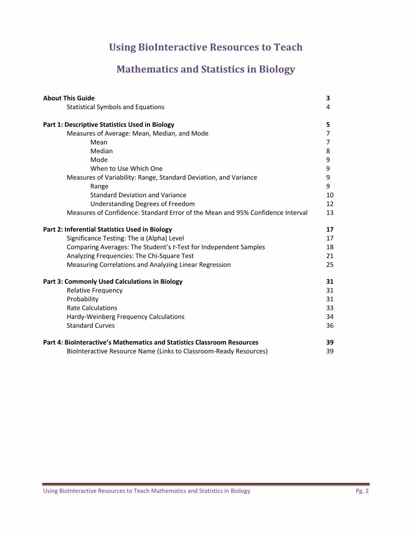
Mathematics and Statistics in Biology About This Guide 3 Statistical Symbols and Equations 4 Part 1: Descriptive Statistics Used in Biology 5
Measures of Average: Mean, Median, and Mode 7 Mean 7 Median 8 Mode 9 When to Use Which One 9 Measures of Variability: Range, Standard Deviation, and Variance 9 Range 9 Standard Deviation and Variance 10 Understanding Degrees of Freedom 12 Measures of Confidence: Standard Error of the Mean and 95% Confidence Interval 13 Part 2: Inferential Statistics Used in Biology 17 Significance Testing: The α (Alpha) Level 17 Comparing Averages: The Student’s t-Test for Independent Samples 18
Analyzing Frequencies: The Chi-Square Test 21 Measuring Correlations and Analyzing Linear Regression 25 Part 3: Commonly Used Calculations in Biology 31 Relative Frequency 31
Probability 31 Rate Calculations 33 Hardy-Weinberg Frequency Calculations 34 Standard Curves 36 Part 4: BioInteractive’s Mathematics and Statistics Classroom Resources 39 BioInteractive Resource Name (Links to Classroom-Ready Resources) 39
Using BioInteractive Resources to Teach Mathematics and Statistics in Biology Pg. 3
About This Guide Many state science standards encourage the use of mathematics and statistics in biology education, including the newly designed AP Biology course, IB Biology, Next Generation Science Standards, and the Common Core. Several resources on the BioInteractive website (www.biointeractive.org), which are listed in the table at the end of this document, make use of math and statistics to analyze research data. This guide is meant to help educators use these BioInteractive resources in the classroom by providing further background on the statistical tests used and step-by-step instructions for doing the calculations. Although most of the example data sets included in this guide are not real and are simply provided to illustrate how the calculations are done, the data sets on which the BioInteractive resources are based represent actual research data.
This guide is not meant to be a textbook on statistics; it only covers topics most relevant to high school biology, focusing on methods and examples rather than theory. It is organized in four parts:
x Part 1 covers descriptive statistics, methods used to organize, summarize, and describe quantifiable
data. The methods include ways to describe the typical or average value of the data and the spread of the data.
x Part 2 covers statistical methods used to draw inferences about populations on the basis of
observations made on smaller samples or groups of the population—a branch of statistics known as inferential statistics.
x Part 3 describes other mathematical methods commonly taught in high school biology, including
frequency and rate calculations, Hardy-Weinberg calculations, probability, and standard curves.
x Part 4 provides a chart of activities on the BioInteractive website that use math and statistics methods. A first draft of the guide was published in July 2014. It has been revised based on user feedback and expert review, and this version was published in October 2015. The guide will continue to be updated with new content and based on ongoing feedback and review.
For a more comprehensive discussion of statistical methods and additional classroom examples, refer to John McDonald’s Handbook of Biological Statistics, http://www.biostathandbook.com, and the College Board’s AP Biology Quantitative Skills: A Guide for Teachers, http://apcentral.collegeboard.com/apc/public/repository/AP_Bio_Quantitative_Skills_Guide-2012.pdf.

Using BioInteractive Resources to Teach Mathematics and Statistics in Biology Pg. 4
Statistical Symbols and Equations
Listed below are the universal statistical symbols and equations used in this guide. The calculations can all be
done using scientific calculators or the formula function in spreadsheet programs.
𝑁: Total number of individuals in a population (i.e., the total number of butterflies of a particular species)
𝑛: Total number of individuals in a sample of a population (i.e., the number of butterflies in a net)
df: The number of measurements in a sample that are free to vary once the sample mean has been
calculated; in a single sample, df = 𝑛 – 1
𝑥 : A single measurement
𝑖: The 𝑖th observation in a sample
6: Summation
�̅�: Sample mean �̅� = ∑
𝑠 : Sample variance 𝑠 = ∑ ( ̅)
𝑠: Sample standard deviation 𝑠 = √𝑠
SEx : Sample standard error, or standard error of the mean (SEM) SE = √
95% CI: 95% confidence interval 95% CI = .√
t-test: tobs = | ̅ ̅ |
Chi-square test (𝑋 ): 𝑋 = ∑ ( )
Linear regression test: 𝑟 = ∑
Hardy-Weinberg principle: p2 + 2pq + q2 = 1.0
Using BioInteractive Resources to Teach Mathematics and Statistics in Biology Pg. 5
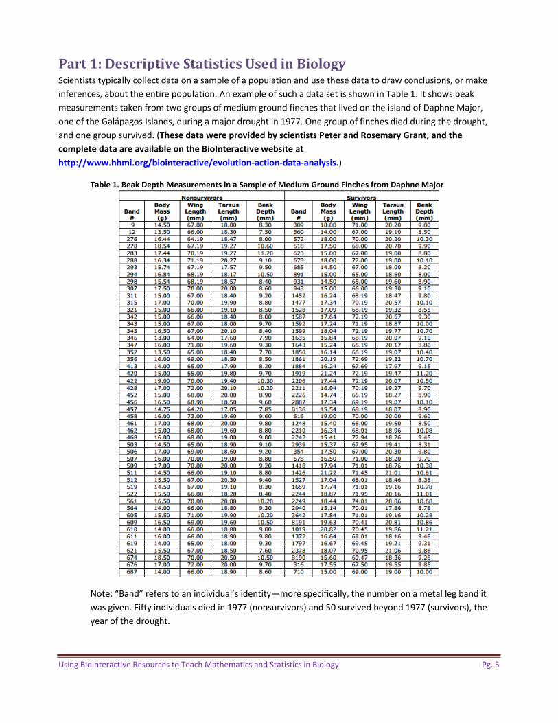
Part 1: Descriptive Statistics Used in Biology Scientists typically collect data on a sample of a population and use these data to draw conclusions, or make inferences, about the entire population. An example of such a data set is shown in Table 1. It shows beak measurements taken from two groups of medium ground finches that lived on the island of Daphne Major, one of the Galápagos Islands, during a major drought in 1977. One group of finches died during the drought, and one group survived. (These data were provided by scientists Peter and Rosemary Grant, and the
complete data are available on the BioInteractive website at
http://www.hhmi.org/biointeractive/evolution-action-data-analysis.)
Table 1. Beak Depth Measurements in a Sample of Medium Ground Finches from Daphne Major
Note: “Band” refers to an individual’s identity—more specifically, the number on a metal leg band it was given. Fifty individuals died in 1977 (nonsurvivors) and 50 survived beyond 1977 (survivors), the year of the drought.

Using BioInteractive Resources to Teach Mathematics and Statistics in Biology Pg. 6
How would you describe the data in Table 1, and what does it tell you about the populations of medium
ground finches of Daphne Major? These are difficult questions to answer by looking at a table of numbers.
One of the first steps in analyzing a small data set like the one shown in Table 1 is to graph the data and examine the distribution. Figure 1 shows two graphs of beak measurements. The graph on the top shows beak
measurements of finches that died during the drought. The graph on the bottom shows beak measurements of
finches that survived the drought.
Be a k D e p ths of 50 Me diu m Groun d Finch es Th a t Did N ot Surviv e th e Droug h t
Be a k D e p ths of 50 Me diu m Groun d Finch es Th a t Surviv e d t h e Droug h t
Figure 1. Distributions of Beak Depth Measurements in Two Groups of Medium Ground Finches Notice that the measurements tend to be more or less symmetrically distributed across a range, with most
measurements around the center of the distribution. This is a characteristic of a normal distribution. Most
statistical methods covered in this guide apply to data that are normally distributed, like the beak
measurements above; other types of distributions require either different kinds of statistics or transforming
data to make them normally distributed.
How would you describe these two graphs? How are they the same or different? Descriptive statistics allows
you to describe and quantify these differences. The rest of Part 1 of this guide provides step-by-step
instructions for calculating mean, standard deviation, standard error, and other descriptive statistics.
Using BioInteractive Resources to Teach Mathematics and Statistics in Biology Pg. 7
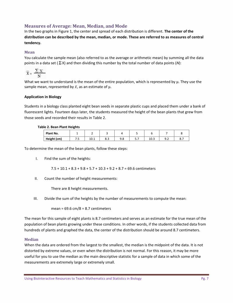
Measures of Average: Mean, Median, and Mode In the two graphs in Figure 1, the center and spread of each distribution is different. The center of the distribution can be described by the mean, median, or mode. These are referred to as measures of central tendency.
Mean You calculate the sample mean (also referred to as the average or arithmetic mean) by summing all the data points in a data set (ΣX) and then dividing this number by the total number of data points (N):
What we want to understand is the mean of the entire population, which is represented by µμ. They use the sample mean, represented by �̅�, as an estimate of µμ.
Application in Biology
Students in a biology class planted eight bean seeds in separate plastic cups and placed them under a bank of
fluorescent lights. Fourteen days later, the students measured the height of the bean plants that grew from
those seeds and recorded their results in Table 2.
Table 2. Bean Plant Heights
Plant No. 1 2 3 4 5 6 7 8
Height (cm) 7.5 10.1 8.3 9.8 5.7 10.3 9.2 8.7
To determine the mean of the bean plants, follow these steps:
I. Find the sum of the heights:
7.5 + 10.1 + 8.3 + 9.8 + 5.7 + 10.3 + 9.2 + 8.7 = 69.6 centimeters
II. Count the number of height measurements: There are 8 height measurements.
III. Divide the sum of the heights by the number of measurements to compute the mean:
mean = 69.6 cm/8 = 8.7 centimeters
The mean for this sample of eight plants is 8.7 centimeters and serves as an estimate for the true mean of the
population of bean plants growing under these conditions. In other words, if the students collected data from
hundreds of plants and graphed the data, the center of the distribution should be around 8.7 centimeters.
Median When the data are ordered from the largest to the smallest, the median is the midpoint of the data. It is not
distorted by extreme values, or even when the distribution is not normal. For this reason, it may be more
useful for you to use the median as the main descriptive statistic for a sample of data in which some of the
measurements are extremely large or extremely small.
Using BioInteractive Resources to Teach Mathematics and Statistics in Biology Pg. 8
To determine the median of a set of values, you first arrange them in numerical order from lowest to highest. The middle value in the list is the median. If there is an even number of values in the list, then the median is the mean of the middle two values.
Application in Biology
A researcher studying mouse behavior recorded in Table 3 the time (in seconds) it took 13 different mice to locate food in a maze.
Table 3. Length of Time for Mice to Locate Food in a Maze
Mouse No. 1 2 3 4 5 6 7 8 9 10 11 12 13
Time (sec.) 31 33 163 33 28 29 33 27 27 34 35 28 32 To determine the median time that the mice spent searching for food, follow these steps:
I. Arrange the time values in numerical order from lowest to highest:
27, 27, 28, 28, 29, 31, 32, 33, 33, 33, 34, 35, 163
II. Find the middle value. This value is the median:
median = 32 seconds In this case, the median is 32 seconds, but the mean is 41 seconds, which is longer than all but one of the mice took to search for food. In this case, the mean would not be a good measure of central tendency unless the really slow mouse is excluded from the data set.
Mode The mode is another measure of the average. It is the value that appears most often in a sample of data. In the example shown in Table 3, the mode is 33 seconds.
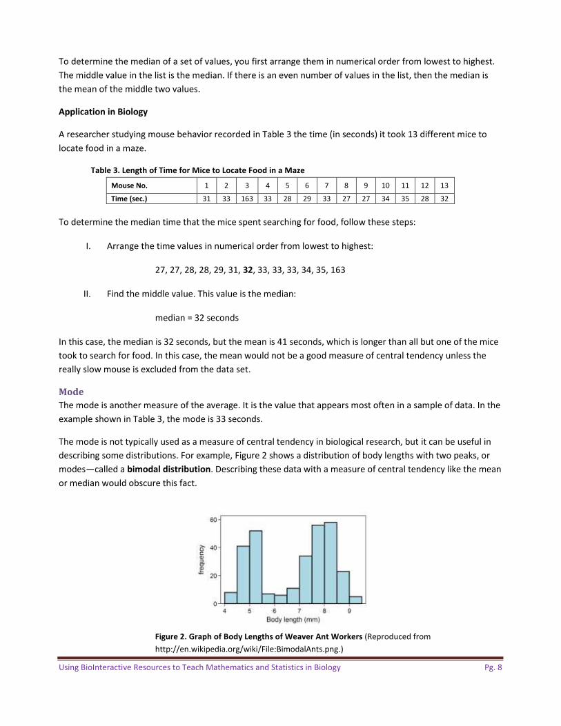
The mode is not typically used as a measure of central tendency in biological research, but it can be useful in describing some distributions. For example, Figure 2 shows a distribution of body lengths with two peaks, or modes—called a bimodal distribution. Describing these data with a measure of central tendency like the mean or median would obscure this fact.
Figure 2. Graph of Body Lengths of Weaver Ant Workers (Reproduced from http://en.wikipedia.org/wiki/File:BimodalAnts.png.)

Using BioInteractive Resources to Teach Mathematics and Statistics in Biology Pg. 9
When to Use Which One The purpose of these statistics is to characterize “typical” data from a data set. You use the mean most often
for this purpose, but it becomes less useful if the data in the data set are not normally distributed. When the
data are not normally distributed, then other descriptive statistics can give a better idea about the typical
value of the data set. The median, for example, is a useful number if the distribution is heavily skewed. For
example, you might use the median to describe a data set of top running speeds of four-legged animals, most
of which are relatively slow and a few, like cheetahs, are very fast. The mode is not used very frequently in
biology, but it may be useful in describing some types of distributions—for example, ones with more than one
peak.
Measures of Variability: Range, Standard Deviation, and Variance Variability describes the extent to which numbers in a data set diverge from the central tendency. It is a
measure of how “spread out” the data are. The most common measures of variability are range, standard deviation, and variance.
Range The simplest measure of variability in a sample of normally distributed data is the range, which is the
difference between the largest and smallest values in a set of data.
Application in Biology
Students in a biology class measured the width in centimeters of eight leaves from eight different maple trees
and recorded their results in Table 4.
Table 4. Width of Maple Tree Leaves
Plant No. 1 2 3 4 5 6 7 8
Width (cm) 7.5 10.1 8.3 9.8 5.7 10.3 9.2 8.7
To determine the range of leaf widths, follow these steps:
I. Identify the largest and smallest values in the data set:
largest = 10.3 centimeters, smallest = 5.7 centimeters
II. To determine the range, subtract the smallest value from the largest value:
range = 10.3 centimeters – 5.7 centimeters = 4.6 centimeters
A larger range value indicates a greater spread of the data—in other words, the larger the range, the greater
the variability. However, an extremely large or small value in the data set will make the variability appear high.
For example, if the maple leaf sample had not included the very small leaf number 5, the range would have
been only 2.8 centimeters. The standard deviation provides a more reliable measure of the “true” spread of
the data.
Using BioInteractive Resources to Teach Mathematics and Statistics in Biology Pg. 10
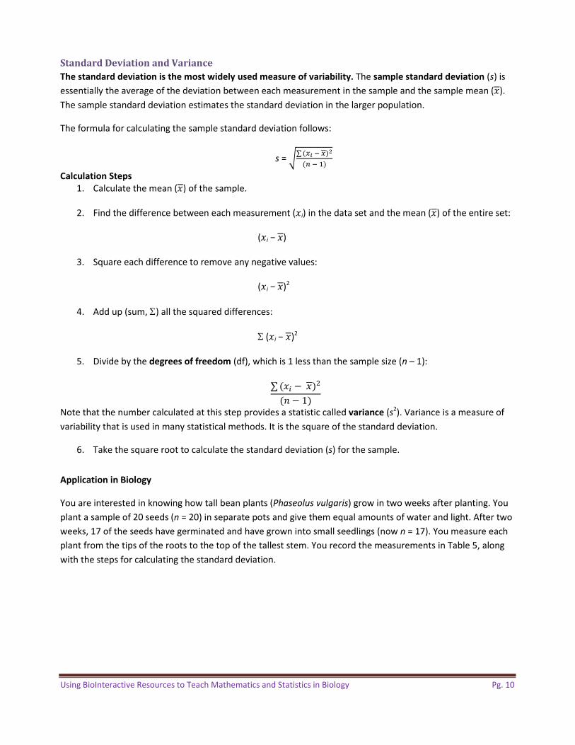
Standard Deviation and Variance The standard deviation is the most widely used measure of variability. The sample standard deviation (s) is essentially the average of the deviation between each measurement in the sample and the sample mean (𝑥). The sample standard deviation estimates the standard deviation in the larger population.
The formula for calculating the sample standard deviation follows:
s = ∑ ( )( )
Calculation Steps 1. Calculate the mean (𝑥) of the sample.
2. Find the difference between each measurement (𝑥i) in the data set and the mean (𝑥) of the entire set:
(𝑥i − 𝑥) 3. Square each difference to remove any negative values:
(𝑥i − 𝑥)2 4. Add up (sum, 6) all the squared differences:
6 (𝑥i − 𝑥)2 5. Divide by the degrees of freedom (df), which is 1 less than the sample size (n – 1):
∑ (𝑥 − 𝑥)(𝑛 − 1)
Note that the number calculated at this step provides a statistic called variance (s2). Variance is a measure of variability that is used in many statistical methods. It is the square of the standard deviation.
6. Take the square root to calculate the standard deviation (s) for the sample.
Application in Biology
You are interested in knowing how tall bean plants (Phaseolus vulgaris) grow in two weeks after planting. You plant a sample of 20 seeds (n = 20) in separate pots and give them equal amounts of water and light. After two weeks, 17 of the seeds have germinated and have grown into small seedlings (now n = 17). You measure each plant from the tips of the roots to the top of the tallest stem. You record the measurements in Table 5, along with the steps for calculating the standard deviation.

Using BioInteractive Resources to Teach Mathematics and Statistics in Biology Pg. 11
Table 5. Plant Measurements and Steps for Calculating the Standard Deviation Plant No. Plant Height (mm) Step 2: (𝑥i − 𝑥)
(mm) Step 3: (𝑥i − 𝑥)2
(mm2) 1 112 (112 – 103) = 9 92 = 81 2 102 (102 – 103) = (−1) (−1)2 = 1
3 106 (106 – 103) = 3 32 = 9
4 120 (120 – 103) = 17 172 = 289
5 98 (98 – 103) = (−5) (−5)2 = 25
6 106 (106 – 103) = 3 32 = 9
7 80 (80 – 103) = (−23) (−23)2 = 529
8 105 (105 – 103) = 2 22 = 4
9 106 (106 – 103) = 3 32 = 9
10 110 (110 – 103) = 7 72 = 49
11 95 (95 – 103) = (−8) (−8)2 = 64
12 98 (98 – 103) = (−5) (−5)2 = 25
13 74 (74 – 103) = (−29) (−29)2 = 841
14 112 (112 – 103) = 9 92 = 81
15 115 (115 – 103) = 12 122 = 144
16 109 (109 – 103) = 6 62 = 36
17 100 (100 – 103) = (−3) (−3)2 = 9 Step 1: Calculate mean. 𝑥 = 103 mm Step 4: ∑ (𝑥i − 𝑥)2
= 2,205
Variance, s2 𝑆𝑡𝑒𝑝 5: ∑ (𝑥i − 𝑥)2/(n – 1) = 2,205/16 = 138
Standard Deviation, s Step 6: √𝑠 = √138 = 11.7 mm
Note: The units for variance are squared units, which make variance less useful as a measure of dispersion.
The mean height of the bean plants in this sample is 103 millimeters ±11.7 millimeters. What does this tell us? In a data set with a large number of measurements that are normally distributed, 68.3% (or roughly two-thirds) of the measurements are expected to fall within 1 standard deviation of the mean and 95.4% of all data points lie within 2 standard deviations of the mean on either side (Figure 3). Thus, in this example, if you assume that this sample of 17 observations is drawn from a population of measurements that are normally distributed, 68.3% of the measurements in the population should fall between 91.3 and 114.7 millimeters and
95.4% of the measurements should fall between 80.1 millimeters and 125.9 millimeters.
Figure 3. Theoretical Distribution of Plant Heights. For normally distributed data, 68.3% of data points lie between ±1 standard deviation of the mean and 95.4% of data points lie between ±2 standard deviations of the mean.

Using BioInteractive Resources to Teach Mathematics and Statistics in Biology Pg. 12
We can graph the mean and the standard deviation of this sample of bean plants using a bar graph with error
bars (Figure 4). Standard deviation bars summarize the variation in the data—the more spread out the individual measurements are, the larger the standard deviation. On the other hand, error bars based on the
standard error of the mean or the 95% confidence interval reveal the uncertainty in the sample mean. They
depend on how spread out the measurements are and on the sample size. (These statistics are discussed
further in “Measures of Confidence: Standard Error of the Mean and 95% Confidence Interval”.)
Figure 4. Mean Plant Height of a Sample of Bean Plants and an Error Bar Representing ±1 Standard Deviation. Roughly two-thirds
of the measurements in this population would be expected to fall
in the range indicated by the bar.
A common misconception is that standard deviation decreases with increasing sample size. As you increase the sample size, standard deviation can either increase or decrease depending on the measurements in the sample. However, with a larger sample size, standard deviation will become a more accurate estimate of the
standard deviation of the population.
Understanding Degrees of Freedom Calculations of sample estimates, such as the standard deviation and variance, use degrees of freedom instead
of sample size. The way you calculate degrees of freedom depends on the statistical method you are using, but
for calculating the standard deviation, it is defined as 1 less than the sample size (n − 1).
To illustrate what this number means, consider the following example. Biologists are interested in the variation
in leg sizes among grasshoppers. They catch five grasshoppers (𝑛 = 5) in a net and prepare to measure the left
legs. As the scientists pull grasshoppers one at a time from the net, they have no way of knowing the leg
lengths until they measure them all. In other words, all five leg lengths are “free” to vary within some general
range for this particular species. The scientists measure all five leg lengths and then calculate the mean to be x
= 10 millimeters. They then place the grasshoppers back in the net and decide to pull them out one at a time
to measure them again. This time, since the biologists already know the mean to be 10, only the first four
measurements are free to vary within a given range. If the first four measurements are 8, 9, 10, and 12
millimeters, then there is no freedom for the fifth measurement to vary; it has to be 11. Thus, once they know
the sample mean, the number of degrees of freedom is 1 less than the sample size, df = 4.

Using BioInteractive Resources to Teach Mathematics and Statistics in Biology Pg. 13
Measures of Confidence: Standard Error of the Mean and 95% Confidence Interval The standard deviation provides a measure of the spread of the data from the mean. A different type of statistic reveals the uncertainty in the calculation of the mean.
The sample mean is not necessarily identical to the mean of the entire population. In fact, every time you take a sample and calculate a sample mean, you would expect a slightly different value. In other words, the sample means themselves have variability. This variability can be expressed by calculating the standard error of the mean (abbreviated as SE ̅ or SEM).
To illustrate this point, assume that there is a population of a species of anole lizards living on an island of the Caribbean. If you were able to measure the length of the hind limbs of every individual in this population and then calculate the mean, you would know the value of the population mean. However, there are thousands of individuals, so you take a sample of 10 anoles and calculate the mean hind limb length for that sample. Another researcher working on that island might catch another sample of 10 anoles and calculate the mean hind limb length for this sample, and so on. The sample means of many different samples would be normally distributed. The standard error of the mean represents the standard deviation of such a distribution and estimates how close the sample mean is to the population mean.
The greater each sample size (i.e., 50 rather than 10 anoles), the more closely the sample mean will estimate the population mean, and therefore the standard error of the mean becomes smaller.
To calculate SE ̅ or SEM divide the standard deviation by the square root of the sample size:
𝑠 = ∑( )( )
SE ̅ = √
What the standard error of the mean tells you is that about two-thirds (68.3%) of the sample means would be within ±1 standard error of the population mean and 95.4% would be within ±2 standard errors.
Another more precise measure of the uncertainty in the mean is the 95% confidence interval (95% CI). For large sample sizes, 95% CI can be calculated using this formula: .
√ , which is typically rounded to √ for ease of calculation. In other words, 95% CI is about twice the standard error of the mean. The actual formula for calculating 95% CI uses a statistic called the t-value for a significance level of 0.05, which is explained in Table 8 in Part 2. For large sample sizes, this t-value is 1.96. Since t-values are not typically covered in high school biology, in this guide we estimate the 95% CI by using 2 x SEM, but note that this is just an approximation. Note about Error Bars: Many bar graphs include error bars, which may represent standard deviation, SEM, or 95% CI. When the bars represent SEM, you know that if you took many samples only about two-thirds of the error bars would include the population mean. This is very different from standard deviation bars, which show how much variation there is among individual observations in a sample. When the error bars represent 95% confidence intervals in a graph, you know that in about 95% of cases the error bars include the population

Using BioInteractive Resources to Teach Mathematics and Statistics in Biology Pg. 14
mean. If a graph shows error bars that represent SEM, you can estimate the 95% confidence interval by making
the bars twice as big—this is a fairly accurate approximation for large sample sizes, but for small samples the
95% confidence intervals are actually more than twice as big as the SEMs.
Application in Biology—Example 1
Seeds of many weed species germinate best in recently disturbed soil that lacks a light-blocking canopy of
vegetation. Students in a biology class hypothesized that weed seeds germinate best when exposed to light. To
test this hypothesis, the students placed a seed from crofton weed (Ageratina adenophora, an invasive species
on several continents) in each of 20 petri dishes and covered the seeds with distilled water. They placed half
the petri dishes in the dark and half in the light. After one week, the students measured the combined lengths
in millimeters of the radicles and shoots extending from the seeds in each dish. Table 6 shows the data and
calculations of variance, standard deviation, standard error of the mean, and 95% confidence interval. The
students plotted the data as two bar graphs showing the standard error of the mean and 95% confidence
interval (Figure 5).
Table 6. Combined Lengths of Crofton Weed Radicles and Shoots after One Week in the Dark and the Light
Petri Dishes Dark (𝒙𝟏) (mm)
Light (𝒙𝟐) (mm)
Dark (𝒙𝒊 − 𝒙𝟏)2
(mm2) Light (𝒙𝒊 − 𝒙𝟐)2
(mm2) 1 and 2 12 18 (12 – 9.6)2 = 5.8 (18 – 18.4)2 = 0.16
3 and 4 8 22 (8 – 9.6)2 = 2.6 (22 – 18.4)2 = 12.96
5 and 6 15 17 (15 – 9.6)2 = 29.1 (17 – 18.4)2 = 1.96
7 and 8 13 23 (13 – 9.6)2 = 11.5 (23 – 18.4)2 = 21.16
9 and 10 6 16 (6 – 9.6)2 = 13.0 (16 – 18.4)2 = 5.76
11 and 12 4 18 (4 – 9.6)2 = 31.4 (18 – 18.4)2 = 0.16
13 and 14 13 22 (13 – 9.6)2 = 11.6 (22 – 18.4)2 = 12.96
15 and 16 14 12 (14 – 9.6)2 = 19.3 (12 – 18.4)2 = 40.96
17 and 18 5 19 (5 – 9.6)2 = 21.1 (19 – 18.4)2 = 0.36
19 and 20 6 17 (6 – 9.6)2 = 13.0 (17 – 18.4)2 = 1.96
∑ (𝑥 − �̅� )2 = 158.4 ∑ (𝑥 − �̅� )2 = 98.4
Mean (�̅�) �̅� = 9.6 (10)
mm �̅� = 18.4 (18)
mm ∑ ( )( ) =
.
∑ ( )( ) =
.
Variance (𝑠 ) 𝑠 = 17.6 𝑠 = 10.93
Standard Deviation, 𝑠 =∑ ( )( ) 𝑠 = 4.20 mm 𝑠 = 3.31 mm
Standard Error of the Mean, SE ̅ = √ SE ̅ = .√ = 1.33 SE ̅ =
.√ = 1.05
95% CI = 𝟐𝒔√𝒏 95% CI = ( . )√ = 2.7 95% CI =
( . )√ = 2.1
Note: The number of replicates (i.e., sample size, n) = 10. Means in parentheses, that is, (10) and (18), are to the nearest millimeter.

Using BioInteractive Resources to Teach Mathematics and Statistics in Biology Pg. 15
Figure 5. Mean Length of Crofton Seedlings after One Week in the Dark or in the Light. The standard error of the mean graph shows the 𝐒𝐄𝒙 as error bars, and the 95% confidence interval graph shows the 𝟗𝟓% 𝐂𝐈 as error bars. (Note that in these calculations we approximated 95% CI as about twice the SEM.) The calculations in Table 6 show that although the students don’t know the actual mean combined radicle and shoot length of the entire population of crofton plants in the dark, it is likely to be a number around the sample mean of 9.6 millimeters ± 1.3 millimeters. For the light treatment it is likely to be 18.4 millimeters ± 1 millimeter. The students can be even more certain that the population mean would be 9.6 millimeters ±2.6 millimeters for the dark treatment and 18.4 millimeters ± 2.1 millimeters for the light treatment.
Note: By looking at the bar graphs, you can see that the means for the light and dark treatments are different. Because the 95% confidence interval error bars do not overlap, this suggests that the true population means are also different. However, in order to determine whether this difference is significant, you will need to conduct another statistical test, the Student’s t-test, which is covered in ”Comparing Averages” in Part 2 of this guide.
Application in Biology—Example 2
A teacher had five students write their names on the board, first with their dominant hands and then with their nondominant hands. The rest of the class observed that the students wrote more slowly and with less precision with the nondominant hand than with the dominant hand. The teacher then asked the class to explain their observations by developing testable hypotheses. They hypothesized that the dominant hand was better at performing fine motor movements than the nondominant hand. The class tested this hypothesis by timing (in seconds) how long it took each student to break 20 toothpicks with each hand. The results of the experiment and the calculations of variance, standard deviation, standard error of the mean, and 95% confidence interval are presented in Table 7. The students then illustrated the data and uncertainty with two bar graphs, one showing the standard error of the mean and the other showing the 95% confidence interval (Figure 6).
Standard Error of the Mean 95% Confidence Interval

Using BioInteractive Resources to Teach Mathematics and Statistics in Biology Pg. 16
Table 7. Number of Seconds It Took for Students to Break 20 Toothpicks with Their Nondominant (ND) and Dominant (D) Hands (number of replicates [n] = 14)
Students ND (𝒙𝟏) (sec.)
D (𝒙𝟐) (sec.)
ND (𝒙𝒊 − 𝒙𝟏)2 D (𝒙𝒊 − 𝒙𝟐)2
Josh 33 37 (33 – 33)2 = 0 (37 – 35)2 = 4
Bobby 24 22 (24 – 33)2 = 81 (22 – 35)2 = 169
Qing 35 37 (35 – 33)2 = 4 (37 – 35)2 = 4
Julie 33 28 (33 – 33)2 = 0 (28 – 35)2 = 49
Lisa 42 50 (42 – 33)2 = 81 (50 – 35)2 = 225
Akash 36 36 (36 – 33)2 = 9 (36 – 35)2 = 1
Hector 31 36 (31 – 33)2 = 4 (36 – 35)2 = 1
Viviana 40 46 (40 – 33)2 = 49 (46 – 35)2 = 121
Brenda 28 26 (28 – 33)2 = 25 (26 – 35)2 = 81
Jane 24 28 (24 – 33)2 = 81 (28 – 35)2 = 49
Asa 23 22 (23 – 33)2 = 100 (22 – 35)2 = 169
Eli 44 52 (44 – 33)2 = 121 (52 – 35)2 = 289
Adee 35 29 (35 – 33)2 = 4 (29 – 35)2 = 36
Jenny 36 37 (36 – 33)2 = 9 (37 – 35)2 = 4
∑ (𝑥 − �̅� )2 = 568 ∑ (𝑥 − �̅� )2 = 1,200
Mean (�̅�) �̅� = 33 �̅� = 35 ∑ ( ̅ ) = ∑ ( ̅ )
= ,
Variance, 𝑠 𝑠 = 44 𝑠 = 92
Standard Deviation, 𝑠 = ∑ ( )( ) 𝑠 = 6.6 sec. 𝑠 = 9.6 sec.
Standard Error of the Mean, SE ̅ = 𝒔√𝒏 SE ̅ = .√ = 1.8 sec. SE ̅ = .
√ = 2.6 sec.
95% CI = 𝟐𝒔√𝒏 95% CI = ( . )√ = 3.5 95% CI = ( . )
√ = 5.1
Figure 6. Mean Number of Seconds for Students to Break 20 Toothpicks with their Nondominant Hands (ND) and Dominant Hands (D). The standard error of the mean graph shows the 𝐒𝐄𝒙 as error bars, and the 95% confidence interval graph shows the 𝟗𝟓% 𝐂𝐈 as error bars.
Standard Error of the Mean 95% Confidence Interval

Using BioInteractive Resources to Teach Mathematics and Statistics in Biology Pg. 17
The calculations indicate that it takes about 31.2 seconds (33 − 1.8) to 34.8 seconds (33 + 1.8) for the
nondominant hand to break toothpicks and about 32.4 to 37.6 seconds for the dominant hand. You can be
more certain that the average for the nondominant hand would fall somewhere between 29.5 seconds (33 –
3.5) and 36.5 seconds (33 + 3.5) and for the dominant hands falls somewhere between 29.9 seconds (35 – 5.1)
and 40.1 seconds (35 + 5.1).
This ends the part on descriptive statistics. Going back to the finch data set in Table 1 and Figure 1 of Part 1,
how would you calculate the sample means for beak sizes of the survivors and nonsurvivors? Is there more
variability among survivors or nonsurvivors? What is the uncertainty in your sample mean estimates? To
find the answers to these questions, see the “Evolution in Action: Data Analysis” activities at
http://www.hhmi.org/biointeractive/evolution-action-data-analysis.
Part 2: Inferential Statistics Used in Biology Inferential statistics tests statistical hypotheses, which are different from experimental hypotheses. To
understand what this means, assume that you do an experiment to test whether “nitrogen promotes plant
growth.” This is an experimental hypothesis because it tells you something about the biology of plant growth.
To test this hypothesis, you grow 10 bean plants in dirt with added nitrogen and 10 bean plants in dirt without
added nitrogen. You find out that the means of these two samples are 13.2 centimeters and 11.9 centimeters,
respectively. Does this result indicate that there is a difference between the two populations and that nitrogen
might promote plant growth? Or is the difference in the two means merely due to chance? A statistical test is
required to discriminate between these possibilities.
Statistical tests evaluate statistical hypotheses. The statistical null hypothesis (symbolized by H0 and
pronounced H-naught) is a statement that you want to test. In this case, if you grow 10 plants with nitrogen
and 10 without, the null hypothesis is that there is no difference in the mean heights of the two groups and
any observed difference between the two groups would have occurred purely by chance. The alternative
hypothesis to H0 is symbolized by H1 and usually simply states that there is a difference between the
populations.
The statistical null and alternative hypotheses are statements about the data that should follow from the
experimental hypothesis.
Significance Testing: The D (Alpha) Level Before you perform a statistical test on the plant growth data, you should determine an acceptable
significance level of the null statistical hypothesis. That is, ask, when do I think my results and thus my test
statistic are so unusual that I no longer think the differences observed in my data are simply due to chance?
This significance level is also known as “alpha” and is symbolized by D.
The significance level is the probability of getting a test statistic rare enough that you are comfortable
rejecting the null hypothesis (H0). (See the “Probability” section of Part 3 for further discussion of probability.)
The widely accepted significance level in biology is 0.05. If the probability (p) value is less than 0.05, you reject
the null hypothesis; if p is greater than or equal to 0.05, you don’t reject the null hypothesis.

Using BioInteractive Resources to Teach Mathematics and Statistics in Biology Pg. 18
Comparing Averages: The Student’s t-Test for Independent Samples The Student’s t-test is used to compare the means of two samples to determine whether they are statistically different. For example, you calculated the sample means of survivor and nonsurvivor finches from
Table 1 and you got different numbers. What is the probability of getting this difference in means, if the
population means are really the same?
The t-test assesses the probability of getting a result more different than the observed result (i.e., the values
you calculated for the means shown in Figure 1) if the null statistical hypothesis (H0) is true. Typically, the null
statistical hypothesis in a t-test is that the mean of the population from which sample 1 came (i.e., the mean
beak size of survivors) is equal to the mean of the population from which sample 2 came (i.e., the mean beak
size of the nonsurvivors), or 𝜇1 = 𝜇2. Rejecting H0 supports the alternative hypothesis, H1, that the means are
significantly different (𝜇1 z 𝜇2). In the finch example, the t-test determines whether any observed differences
between the means of the two groups of finches (9.67 millimeters versus 9.11 millimeters) are statistically
significant or have likely occurred simply by chance.
A t-test calculates a single statistic, t, or tobs, which is compared to a critical t-statistic (tcrit):
tobs = | ̅ ̅ |
To calculate the standard error (SE) specific for the t-test, we calculate the sample means and the variance (s2)
for the two samples being compared—the sample size (n) for each sample must be known:
SE = +
Thus, the complete equation for the t-test is
tobs = | ̅ ̅ |
Calculation Steps 1. Calculate the mean of each sample population and subtract one from the other. Take the absolute
value of this difference.
2. Calculate the standard error, SE. To compute it, calculate the variance of each sample (s2), and divide it
by the number of measured values in that sample (n, the sample size). Add these two values and then
take the square root.
3. Divide the difference between the means by the standard error to get a value for t. Compare the
calculated value to the appropriate critical t-value in Table 8. Table 8 shows tcrit for different degrees of
freedom for a significance value of 0.05. The degrees of freedom is calculated by adding the number of data points in the two groups combined, minus 2. Note that you do not have to have the same
number of data points in each group.
4. If the calculated t-value is greater than the appropriate critical t-value, this indicates that you have
enough evidence to support the hypothesis that the means of the two samples are significantly
different at the probability value listed (in this case, 0.05). If the calculated t is smaller, then you
cannot reject the null hypothesis that there is no significant difference.

Using BioInteractive Resources to Teach Mathematics and Statistics in Biology Pg. 19
Table 8. Critical t-Values for a Significance Level D = 0.05
Degrees of Freedom (df) tcrit (D = 0.05) 1 12.71 2 4.30 3 3.18 4 2.78 5 2.57 6 2.45 7 2.36 8 2.31 9 2.26 10 2.23 11 2.20 12 2.18 13 2.16 14 2.14 15 2.13 16 2.12 17 2.11 18 2.10 19 2.09 20 2.09 21 2.08 22 2.07 23 2.07 24 2.06 25 2.06 26 2.06 27 2.05 28 2.05 29 2.04 30 2.04 40 2.02 60 2.00 120 1.98 Infinity 1.96
Note: There are two basic versions of the t-test. The version presented here assumes that each sample was
taken from a different population, and so the samples are therefore independent of one another. For example,
the survivor and nonsurvivor finches are different individuals, independent of one another, and therefore
considered unpaired. If we were comparing the lengths of right and left wings on all the finches, the samples
would be classified as paired. Paired samples require a different version of the t-test known as a paired t-test,
a version to which many statistical programs default. The paired t-test is not discussed in this guide.
Application in Biology
After a small population of crayfish was accidentally released into a shallow pond, biologists noticed that the
crayfish had consumed nearly all of the underwater plant population; aquatic invertebrates, such as the water
flea (Daphnia sp.), had also declined. The biologists knew that the main predator of Daphnia is the goldfish,
and they hypothesized that the underwater plants protected the Daphnia from the goldfish by providing hiding
places. The Daphnia lost their protection as the underwater plants disappeared. The biologists designed an

Using BioInteractive Resources to Teach Mathematics and Statistics in Biology Pg. 20
experiment to test their hypothesis. They placed goldfish and Daphnia together in a tank with underwater
plants, and an equal number of goldfish and Daphnia in another tank without underwater plants. They then
counted the number of Daphnia eaten by the goldfish in 30 minutes. They replicated this experiment in nine
additional pairs of tanks (i.e., sample size = 10, or n = 10, per group). The results of their experiment and their
calculations of experimental error (variance, s2) are in Table 9.
Experimental hypothesis: The underwater plants protect Daphnia from goldfish by providing hiding places. Experimental prediction: By placing Daphnia and goldfish in tanks with and without plants, you should see a
difference in the survival of Daphnia in the two tanks.
Statistical null hypothesis: There is no difference in the number of Daphnia in tanks with plants compared to tanks without plants: any difference between the two groups occurs simply by chance.
Statistical alternative hypothesis: There is a difference in the number of Daphnia in tanks with plants
compared to tanks without plants.
Table 9. Number of Daphnia Eaten by Goldfish in 30 Minutes in Tanks with or without Underwater Plants Tanks Plants
(sample1) No Plants (sample2)
Plants (𝒙𝒊 − 𝒙𝟏)2
No Plants (𝒙𝒊 − 𝒙𝟐)2
1 and 2 13 14 (9.6 – 13)2 = 11.56 (14.4 – 14)2 = 0.16
3 and 4 9 12 (9.6 – 9)2 = 0.36 (14.4 – 12)2 = 5.876
5 and 6 10 15 (9.6 – 10)2 = 0.16 (14.4 – 15)2 = 0.436
7 and 8 10 14 (9.6 – 10)2 = 0.16 (14.4 – 14)2 = 0.16
9 and 10 7 17 (9.6 – 7)2 = 6.76 (14.4 – 17)2 = 6.76
11 and 12 5 10 (9.6 – 5)2 = 21.16 (14.4 – 10)2 = 19.37
13 and 14 10 15 (9.6 – 10)2 = 0.16 (14.4 – 15)2 = 0.36
15 and 16 14 15 (9.6 – 14)2 = 19.34 (14.4 – 15)2 = 0.36
17 and 18 9 18 (9.6 – 9)2 = 0.36 (14.4 – 18)2 = 12.96
19 and 20 9 14 (9.6 – 9)2 = 0.36 (14.4 – 14)2 = 0.16
∑ (𝑥 − �̅� )2 = 60.4 ∑ (𝑥 − �̅� )2 = 46.4
Mean, �̅� �̅� = 9.6 �̅� = 14.4 ∑ ( ̅ ) =
.
∑ ( ̅ ) =
.
Variance, 𝑠 𝑠 = 6.71 𝑠 = 5.16
To determine whether the difference between the two groups was significant, the biologists calculated a t-test
statistic, as shown below:
SE = + = . + .
= 1.089
The mean difference (absolute value) = |�̅� − �̅� | = |9.6 − 14.4| = 4.8
t = | ̅ ̅ |
= .
. = 4.41
There are (10 + 10 − 2) = 18 degrees of freedom, so the critical value for p = 0.05 is 2.10 from Table 8. The
calculated t-value of 4.41 is greater than 2.10, so the students can reject the null hypothesis that the
differences in the numbers of Daphnia eaten in the presence or absence of underwater plants were accidental.

Using BioInteractive Resources to Teach Mathematics and Statistics in Biology Pg. 21
So what can they conclude? It is possible that the goldfish ate significantly more Daphnia in the absence of
underwater plants than in the presence of the plants.
Analyzing Frequencies: The Chi-Square Test The t-test is used to compare the sample means of two sets of data. The chi-square test is used to determine
how the observed results compare to an expected or theoretical result.
For example, you decide to flip a coin 50 times. You expect a proportion of 50% heads and 50% tails. Based on
a 50:50 probability, you predict 25 heads and 25 tails. These are the expected values. You would rarely get
exactly 25 and 25, but how far off can these numbers be without the results being significantly different from
what you expected? After you conduct your experiment, you get 21 heads and 29 tails (the observed values). Is
the difference between observed and expected results purely due to chance? Or could it be due to something
else, such as something might be wrong with the coin? The chi-square test can help you answer this question.
The statistical null hypothesis is that the observed counts will be equal to that expected, and the alternative
hypothesis is that the observed numbers are different from the expected.
Note that this test must be used on raw categorical data. Values need to be simple counts, not percentages or
proportions. The size of the sample is an important aspect of the chi-square test—it is more difficult to detect
a statistically significant difference between experimental and observed results in a small sample than in a
large sample. Two common applications of this test in biology are in analyzing the outcomes of a genetic cross
and the distribution of organisms in response to an environmental factor of interest.
To calculate the chi-square test statistic (χ2), you use the equation
𝜒 = ∑ ( )
o = observed values e = expected values
χ2 = chi-square value
6 = summation Calculation Steps
1. Calculate the chi-square value. The columns in Table 10 outline the steps required to calculate the chi-square value and test the null hypothesis, using the coin-flipping example discussed above. The equations for calculating a chi-square value are provided in each column heading.
Table 10. Coin-Toss Chi-Square Value Calculations
Side of Coin Observed (o) Expected (e) (o − e) (o − e)2 (o − e)2/e Heads 21 25 (−4) 16 0.64
Tails 29 25 4 16 0.64
χ2 = ∑ (o − e)2/e → χ2
= 1.28
2. Determine the degrees of freedom value as follows:
df = number of categories − 1
In the example above, there are two categories (heads and tails):
df = (2 − 1) = 1

Using BioInteractive Resources to Teach Mathematics and Statistics in Biology Pg. 22
3. Use the critical values table (Table 11) to determine the probability (p) value. A p-value of 0.05 (which is shown in red in Table 11) means there is only a 5% probability of getting the observed difference between observed and expected values by chance, if the null hypothesis is true (i.e., there is no real difference).
For example, for df = 1, there is a 5% probability (p-value = 0.05) of obtaining a χ2-value of 3.841 or larger by
chance. If the χ2-value obtained was 4.5, then you can reject the null hypothesis that there is no real difference
between observed and expected data. The difference between observed and expected data is likely real and is
considered statistically significant.
If the χ2-value was 3.1, then you cannot reject the null hypothesis. The difference between observed and
expected data may be accidental and is not statistically significant.
Significance testing in biology typically uses a p-value of 0.05, which is also referred to as the alpha value (see
“Significance Testing: The α (Alpha) Level” in Part 2). A result with the p-value of 0.05 or lower is deemed a statistically significant result.
To use the critical values table (Table 11), locate the calculated χ2-value in the row corresponding to the
appropriate number of degrees of freedom. For the coin-flipping example, locate the calculated χ2-value in the
df = 1 row. The χ2-value obtained was 1.28, which falls between 0.455 and 2.706 and is smaller than 3.841 (the
χ2-value at the p = 0.05 cutoff); in other words, the result was likely to happen between 10% and 50% of time.
Therefore, you cannot reject the null hypothesis that the results have likely occurred simply by chance, at an
acceptable significance level.
Table 11. Critical Values Table for Different Significance Levels and Degrees of Freedom
Application in Biology—Example 1
Students just learned in their biology class that pill bugs use gill-like structures to breathe oxygen. The students
hypothesized that the pill bugs’ gills require them to live in wet environments for their survival. To test the
hypothesis, they wanted to determine whether pill bugs show a preference for living in wet or dry
environments.
The students placed 15 pill bugs on the dry side of a two-sided choice chamber, and 15 pill bugs on the wet
side of the chamber. Fifteen minutes later, 26 pill bugs were on the wet side and 4 on the dry side. The data
are shown in Table 12.
Table 12. Pill Bug Locations on Two-Sided Chamber Elapsed Time (min.) Pill Bugs on Wet Side (no.) Pill Bugs on Dry Side (no.)
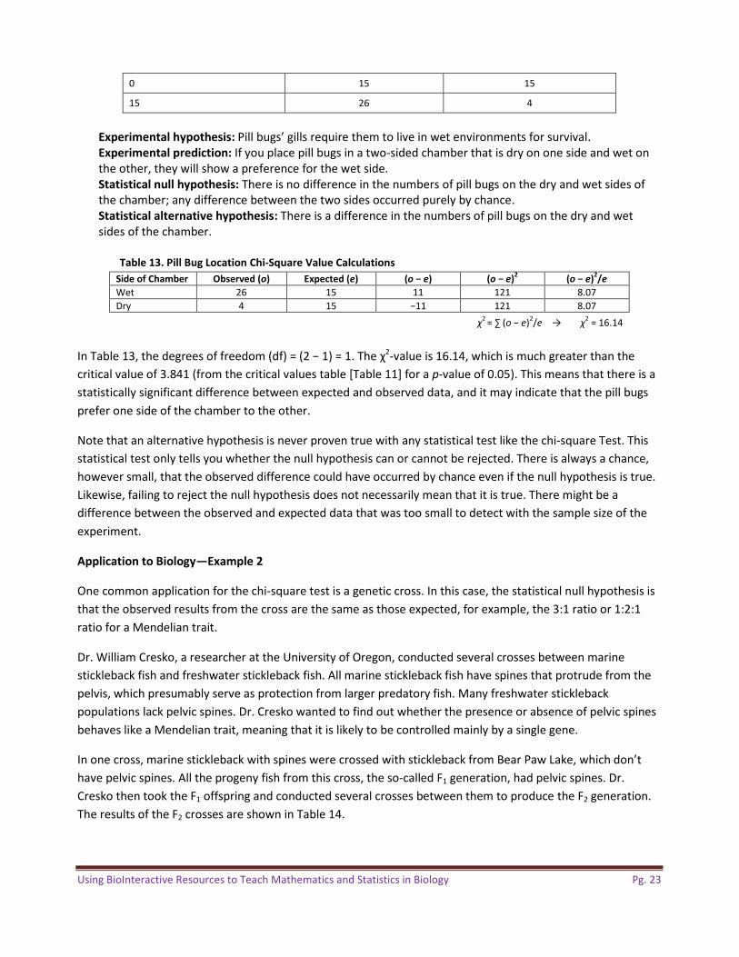
Using BioInteractive Resources to Teach Mathematics and Statistics in Biology Pg. 23
0 15 15
15 26 4
Experimental hypothesis: Pill bugs’ gills require them to live in wet environments for survival. Experimental prediction: If you place pill bugs in a two-sided chamber that is dry on one side and wet on the other, they will show a preference for the wet side. Statistical null hypothesis: There is no difference in the numbers of pill bugs on the dry and wet sides of the chamber; any difference between the two sides occurred purely by chance. Statistical alternative hypothesis: There is a difference in the numbers of pill bugs on the dry and wet sides of the chamber.
Table 13. Pill Bug Location Chi-Square Value Calculations Side of Chamber Observed (o) Expected (e) (o − e) (o − e)2 (o − e)2/e Wet 26 15 11 121 8.07 Dry 4 15 −11 121 8.07
χ2 = ∑ (o − e)2/e → χ2 = 16.14
In Table 13, the degrees of freedom (df) = (2 − 1) = 1. The χ2-value is 16.14, which is much greater than the
critical value of 3.841 (from the critical values table [Table 11] for a p-value of 0.05). This means that there is a
statistically significant difference between expected and observed data, and it may indicate that the pill bugs
prefer one side of the chamber to the other.
Note that an alternative hypothesis is never proven true with any statistical test like the chi-square Test. This
statistical test only tells you whether the null hypothesis can or cannot be rejected. There is always a chance,
however small, that the observed difference could have occurred by chance even if the null hypothesis is true.
Likewise, failing to reject the null hypothesis does not necessarily mean that it is true. There might be a
difference between the observed and expected data that was too small to detect with the sample size of the
experiment.
Application to Biology—Example 2
One common application for the chi-square test is a genetic cross. In this case, the statistical null hypothesis is
that the observed results from the cross are the same as those expected, for example, the 3:1 ratio or 1:2:1
ratio for a Mendelian trait.
Dr. William Cresko, a researcher at the University of Oregon, conducted several crosses between marine
stickleback fish and freshwater stickleback fish. All marine stickleback fish have spines that protrude from the
pelvis, which presumably serve as protection from larger predatory fish. Many freshwater stickleback
populations lack pelvic spines. Dr. Cresko wanted to find out whether the presence or absence of pelvic spines
behaves like a Mendelian trait, meaning that it is likely to be controlled mainly by a single gene.
In one cross, marine stickleback with spines were crossed with stickleback from Bear Paw Lake, which don’t have pelvic spines. All the progeny fish from this cross, the so-called F1 generation, had pelvic spines. Dr.
Cresko then took the F1 offspring and conducted several crosses between them to produce the F2 generation.
The results of the F2 crosses are shown in Table 14.

Using BioInteractive Resources to Teach Mathematics and Statistics in Biology Pg. 24
Table 14. F2 Generation: Cross of F1 Generation Individuals Cross Nu mb er Tot al N um b er of F2 Fish F2 Fish wit h Spines F2 Fish wit hout Spin es 1 98 71 27 2 79 62 17 3 62 49 13 4 34 28 6 5 29 24 5 6 23 17 6 7 21 17 4 8 19 18 1 9 15 11 4 10 12 10 2 11 12 10 2 12 4 3 1 Total 408 320 88
Source: Cresko, William A., A. Amores, C. Wilson, J. Murphy, M. Currey, P. Phillips, M. Bell, C. Kimmel,
and J. Postlethwait. “Parallel Genetic Basis for Repeated Evolution of Armor Loss in Alaskan Threespine
Stickleback Populations.” Proceedings of the National Academy of Sciences of the United States of America 101 (2004): 6050–6055.
If the presence of pelvic spines is controlled by a single gene and the presence of pelvic spines is the dominant
trait as suggested by the F1 results, you would expect a ratio of 3:1 for fish with pelvic spines to fish without
pelvic spines in the F2 generation. For a total of 408 fish, the expected results would be 306:102. The results
from Dr. Cresko’s crosses are 320:88.
The null hypothesis is that there is no real difference between the expected results and the observed results,
and that the difference that we see occurred purely by chance. The statistical alternative hypothesis is that
there is a real difference between observed and expected results.
Table 15. Stickleback Spine Chi-Square Value Calculations Phenotype Observed (o) Expected (e) (o − e) (o − e)2 (o − e)2/e Spines present 320 306 14 196 0.64
Spines absent 88 102 −14 196 0.64
χ2 = ∑ (o − e)2/e → χ2
= 1.28
The χ2-value is 1.28, which is less than the critical value of 3.841 (from the critical values table [Table 11] for a
p-value of 0.05 and a df of 1). This means that the difference between expected and observed data is not
statistically significant. Based on this calculation, we cannot reject the null hypothesis and conclude that any
difference between observed and expected results may have occurred simply by chance.
The chi-square example above is provided in the BioInteractive activity “Using Genetic Crosses to Analyze a
Stickleback Trait,” http://www.hhmi.org/biointeractive/using-genetic-crosses-analyze-stickleback-trait.
Another application of chi-square to genetics is available in the activity “Mapping Genes to Traits in Dogs Using SNPs,” http://www.hhmi.org/biointeractive/mapping-traits-in-dogs.