Mathematics and Mechanics of Solids Stress-driven solution

Article

Stress-driven solution torate-independent elasto-plasticitywith damage at small strains and itscomputer implementation

Mathematics and Mechanics of Solids1–21© The Author(s) 2016Reprints and permissions:sagepub.co.uk/journalsPermissions.navDOI: 10.1177/1081286515627674mms.sagepub.com

Tomáš RoubícekMathematical Institute, Charles University, Prague, Czech RepublicInstitute of Thermomechanics, Czech Academy of Sciences, Prague, Czech RepublicInstitute of Information Theory and Automation, Czech Academy of Sciences, Prague, Czech Republic

Jan ValdmanInstitute of Information Theory and Automation, Czech Academy of Sciences, Prague, Czech RepublicInstitute of Mathematics and Biomathematics, Faculty of Science, University of South Bohemia, CzechRepublic

Received 03 June 2015; accepted 16 December 2015

AbstractQuasistatic rate-independent damage combined with linearized plasticity with hardening at small strains is investigated.Fractional-step time discretization is devised with the purpose of obtaining a numerically efficient scheme, possibly con-verging to a physically relevant stress-driven solution, which however is to be verified a posteriori using a suitableintegrated variant of the maximum-dissipation principle. Gradient theories both for damage and for plasticity are con-sidered to make the scheme numerically stable with guaranteed convergence within the class of weak solutions. Afterfinite-element approximation, this scheme is computationally implemented and illustrative 2-dimensional simulations areperformed.

KeywordsRate-independent systems, nonsmooth continuum mechanics, incomplete ductile damage, linearized plasticity withhardening, quasistatic rate-independent evolution, local solutions, maximum dissipation principle, fractional-step timediscretization, quadratic programming

1. IntroductionA combination of plasticity and damage, also called ductile damage, opens colorful scenarios with importantapplications in civil or mechanical engineering. These have interesting mathematical problems, in particularwhen compared with plasticity or damage alone. Often, both plastification and damage processes are muchfaster than the rate of applied load and, in a basic scenario, any internal time scale is neglected and the mentionedinelastic processes are considered to be rate independent. The goal of this article is to devise a model togetherwith its efficient computational approximation that would lead to a numerical stable and convergent scheme

Corresponding author:Tomáš Roubícek, Mathematical Institute, Charles University, Sokolovska, 83 Prague CZ-18675, Czech Republic.Email: [email protected]

at TULANE UNIV on April 11, 2016mms.sagepub.comDownloaded from

http://mms.sagepub.com/

2 Mathematics and Mechanics of Solids

and, at least in particular situations, calculate physically relevant solutions of a stress-driven type, verifiable aposteriori by checking a suitable version of the maximum-dissipation principle.

We use the very standard linearized, associative, plasticity at small strain as presented in [1]. Simultaneously,we use also a rather standard scalar (i.e. isotropic) damage as presented in [2]. We have primarily in minda conventional engineering model with unidirectional evolution of damage; in fact, healing will be allowedfor analytical reasons, although is expected to be ineffective in the usual applications, see Remark 2.1 below.All rate-dependent phenomena (as inertia or heat conduction and thermo-coupling) are neglected; this meansthe problem is considered to be quasistatic and fully rate-independent. To avoid serious mathematical andcomputational difficulties, we have in mind an incomplete damage.

The aforementioned modeling simplification leading to a quasistatic rate-independent system, which reflectscertain well-motivated asymptotics, brings serious questions and difficulties. This is because the class of rea-sonably general solutions is very wide if the governing energy is not convex (as necessary here) and involvessolutions of a very different nature, some of which are physically not relevant [3,4]. In particular, to avoid theunwanted effects of unrealistically easy damage under subcritical stress, one cannot require energy conserva-tion and thus cannot consider so-called energetic solutions [5]. This concept is, however, occasionally used fordamage with plasticity in purely mathematically-focused literature [6–8]. This is related to the discussion onwhether energy or stress is responsible for governing the evolution of rate-independent systems [9].

In contrast to the aforementioned energetic solutions (which allow for simpler analysis without consideringgradient plasticity, but lead to recursive global-minimization problems which are difficult to realize and mayslide to scenarios of unrealistic early damage), we will focus here on solutions that are stress-driven and that canbe efficiently obtained numerically. We will rely on careful usage of a suitable integral-version of the maximum-dissipation principle, as devised in [10] and used, rather heuristically, in engineering models of damage withplasticity and hardening, see [11]. This brings specific difficulties with convergence (which requires the use ofgradient plasticity) and specific a posteriori verification of a suitable approximate version of the aforementionedmaximum-dissipation principle. This was suggested in [10, Remark 4.6] for damage itself, and is modifiedhere for the combination of damage and plasticity (analogous to [12]) for a surface variant of the elasto-plasto-damage model. If the maximum-dissipation principle holds (at least with a good accuracy) we can claim thatthe numerically obtained solution is physically relevant as stress-driven (with a good accuracy).

A more physically justified and better motivated approach would be to involve a small viscosity to thedamage variable or to the elastic and plastic strains, and then to pass these viscosities to zero. The limits obtainedin this way are called vanishing-viscosity solutions to the original rate-independent system, and both theiranalysis and computer implementation are very difficult: for models without plasticity [13], for viscosity indamage or for viscosity in elastic strain [14].

In principle, there are two basic scenarios for how the material might respond to an increasing loading:either it will first plasticize and then go into damage due to hardening effects, or it will first go into damage andthen plasticize; of course, various intermediate scenarios are possible too. The latter scenario needs a damage-influenced yield stress and must allow for no hardening (and in particular perfect plasticity), see [15]. Let usonly remark that a damage-dependence of the yield stress in the fully rate-independent setting would make thedissipation state-dependent, which brings serious difficulties as seen in [4, Section 3.2] and, for the particularelasto-plasto-damage model, in [6–8]. In this paper, we will concern ourselves exclusively with the formerscenario, in particular that damage does not influence the yield stress. Moreover, we will consider only kinematichardening, although all the considerations could easily be augmented by isotropic hardening, too. Anotheressential difference from reference [15] is that, as already explained, the energy is intentionally not conservedhere.

The plan of the paper is as follows: in Section 2 we devise the model in its classical formulation and then,in Section 3, its suitable weak formulation by discussing stress-driven solutions and the role of the maximum-dissipation principle. In Section 4, we propose a constructive time discretization method and prove its numericalstability (i.e. a priori estimates) and convergence towards weak solutions. After a further finite-element dis-cretization outlined in Section 5, this allows for efficient computer implementation of the model, which isdemonstrated on illustrative 2-dimensional examples in Section 6.

2. The model and its weak formulationHereafter, we suppose that the damageable elasto-plastic body occupies a bounded Lipschitz domain � ⊂ R

d,d = 2 or 3. We denote �n the outward unit normal to ∂�. We further suppose that the boundary of � splits as

∂� := � = �D ∪ �N ,



Roubícek and Valdman 3

Table 1. Summary of the basic notation used through the paper.

d = 2, 3 dimension of the problem, eel : Q → Rd×dsym elastic strain,

Rd×dsym := {A ∈ R

d×d ; A = A�}, e = e(u) = eel+π = 12∇u�+ 1

2∇u totalR

d×ddev := {A ∈ R

d×dsym ; tr A = 0}, small-strain tensor,

u : Q → Rd displacement, C : [0, 1] → R

34elasticity tensor (dependent on ζ ),

π : Q → Rd×ddev plastic strain, H ∈ R

34hardening tensor (independent of ζ ),

ζ : Q → [0, 1] damage variable, S ⊂ Rd×ddev the elastic domain (convex, int S 0),

a > 0 activation energy for damage, wD : �D → Rd prescribed boundary displacement,

f :�N → Rd applied traction force, κ1 > 0 scale coefficient of the gradient of plasticity,

g:Q → Rd applied bulk force (as gravity), κ2 > 0 scale coefficient of the gradient of damage,

σel : Q → Rd×dsym elastic stress, b > 0 activation energy for possible healing.

with �D and �N open subsets in the relative topology of ∂�, disjoint one from each other and, up to (d−1)-dimensional zero measure, covering ∂�. Later, the Dirichlet or the Neumann boundary conditions will beprescribed on �D and �N, respectively. Considering T > 0 a fixed time horizon, we set

I := [0, T], Q := (0, T)×�, � := I×�, �D := I×�D, �N := I×�N.

Further, Rd×dsym and R

d×ddev will denote the set of symmetric or symmetric trace-free (= deviatoric) (d×d)-matrices,

respectively. For readers’ convenience, let us summarize the basic notation used in Table 1.The state is formed by the triple q := (u, π , ζ ). The governing equation/inclusions read as

div σel + g = 0 with σel = C(ζ )eel and eel = e(u)−π , (momentum equilibrium) (2.1a)

∂δ∗S (

.π) dev σel − Hπ + κ1�π , (plastic flow rule) (2.1b)

∂δ∗[−a,b](

.ζ ) −1

2C

′(ζ )eel : eel + κ2 div(|∇ζ |r−2∇ζ

) − N[0,1](ζ ), (damage flow rule) (2.1c)

with δS the indicator function to S and δ∗S its convex conjugate and with “dev” denoting the deviatoric part of a

tensor, i.e. dev A := A − tr A/d. Here, [C(ζ )e]ij means∑d

k,l=1 Cijkl(ζ )ekl.Of course, (2.1) is to be completed by appropriate boundary conditions, e.g.

u = wD on �D, (2.2a)

σel·�n = f on �N, (2.2b)

∇π�n = 0 and ∇ζ ·�n = 0 on � (2.2c)

with �n denoting the unit outward normal to �. We will consider an initial-value problem for equations (2.1)–(2.2) by asking for

u(0) = u0, π(0) = π0, and ζ (0) = ζ0. (2.3)

In fact, as.u does not occur in equation (2.1), u0 is rather formal and its only qualification is to make

E (0, u0, π0, ζ0) finite not to degrade the energy balance in equation (3.1d) on [0, t].Let us note that the homogeneous Neumann condition (2.2a) for both π and ζ is a standard first choice,

reflecting the usual situation that the coefficients κ1 > 0 and κ2 > 0 are small and not reliably known, and shouldprimarily determine the length scale inside the specimen (while even less is known about the surface). As fordamage, prescribing a flux jdam = κ2|∇ζ |r−2∇ζ ·�n on � is sometimes considered as a model for some erosiondue to the influence of the outer severe environment. Alternatively, a Dirichlet condition ζ = 1 on � wouldreflect that the damage may occur only inside while the surface is damage-free by some special technologicaltreatment. Both modifications do not make particular difficulties for analysis or numerical implementation, thelatter one making some aspects even simpler.




After considering an extension uD = uD(t) of wD(t) from equation (2.2a) on the whole domain �, it isconvenient to make a substitution of u + uD instead of u into equations (2.1)–(2.2), and we arrive at the problemwith time-constant (even homogeneous) Dirichlet boundary conditions. More specifically,

eel in equation (2.1b) replaced by eel = e(u+uD)−π , and (2.4a)

wD in equation (2.2a) replaced by 0. (2.4b)

Assuming (C(ζ )e(uD)·�n = 0 on �N for any admissible ζ , this transformation will keep f in equation (2.2b)unchanged.

Actually, equation (2.1b) represents the thermodynamical force-balance governing damage evolution, whilethe corresponding flow rule is written in the (equivalent) form

.π ∈ NS

(dev σel − Hπ − κ1�π

)with σel = C(ζ )eel (2.5)

with NS denoting the set-valued normal-cone mapping to the convex set S. An analogous remark applies toequation (2.1c). The system (2.1) with the boundary conditions (2.2) has, in its weak formulation, the structureof an abstract Biot-type equation (or rather, here, inclusion, e.g. [4, 16, 17]):

∂ .qR(

.q) + ∂qE (t, q) 0 (2.6)

with suitable time-dependent stored-energy functional E and the state-dependent potential of dissipative forcesR. Equally, as already used in equation (2.5), one can write equation (2.6) as a generalized gradient flow

.q ∈ ∂ξR

∗( − ∂E (t, q))

(2.7)

where R∗ denotes the conjugate functional. The governing functionals corresponding to equations (2.1)–(2.2)after the transformation (2.4) are

E (t, u, π , ζ ) :=∫

�

1

2C(ζ )

(e(u+uD(t))−π

):(e(u+uD(t))−π

) + 1

2Hπ : π

+ κ1

2|∇π |2+ κ2

r|∇ζ |r+ δ[0,1](ζ ) − g(t)·u dx −

∫�N

f (t)·u dS, (2.8a)

R(.π ,

.ζ ) ≡ R1(

.π) + R2(

.ζ ) :=

∫�

δ∗S (

.π) + a

.ζ− + b

.ζ+ dx (2.8b)

where z+ := max(z, 0) and z− := max(−z, 0) ≥ 0. Note that the damage does not affect the hardening, whichreflects the idea that, on the microscopic level, damage in the material that underwent hardening develops byevolving microcracks and even a completely damaged material consists of micro-pieces that bear the hardeningenergy 1

2Hπ : π stored before. This model preserves coercivity of hardening even under complete damage,however the analysis below admits only incomplete damage. If ζ �→ C(ζ )e:e is strictly convex for any e �= 0,we speak about a cohesive damage which exhibits a certain hardening effect so that the required driving forceincreases when damage is to be accomplished. We can thus model quite a realistic response to various loadingexperiments, as shown schematically in Figure 1 for the case of a possible complete damage (whose analysisremains open, however). Note that, due to the “incompressibility” constraint tr π = 0, no plastification istriggered under a pure tension or compression loading.

Let us further note that (u, π) �→ E (t, u, π , ζ ) is smooth so that ∂qE = {E ′u} × {E ′

π } × ∂ζE with E ′u and E ′

π

denoting the respective partial Gâteaux derivatives. Equation (2.6) can thus be written more specifically as thesystem

E ′u(t, u, π , ζ ) = 0, (2.9a)

∂R1(.π) + E ′

π (t, u, π , ζ ) 0, (2.9b)

∂R2(.ζ ) + ∂ζE (t, u, π , ζ ) 0. (2.9c)




Figure 1. Schematic response of the stress σel to the total strain e during a “one-dimensional” tension (left) or shear (right) loadingexperiment under a stress-driven scenario. The former option does not exhibit any plastification because the trace-free plastic strain(valued in R

d×ddev ) ignores tension/compression. The latter option combines plasticity with eventual complete damage. Dashed lines

outline a response to unloading, C = C(ζ ) refers to the Young’s modulus (left) or the shear modulus (right).

Remark 2.1 (Irreversible damage in engineering models). Usual engineering models consider b = ∞, i.e. nohealing is allowed. In fact, due to an essentially missing driving force for healing, our modification b < ∞would not have any influence on the evolution if it were not any ∇ζ -term in the stored energy. Thus, if thehealing threshold b is big and the gradient-term coefficient κ2 > 0 is small, we expect to have essentially(usually desired) unidirectional evolution as far as the damage concerns.

Remark 2.2 (Surface variant of the damage/plasticity). A similar scenario distinguishing tension (which leadsto damage without plastification) and shear (with plastifying the material before damage) as in Figure 1 wasused in a surface variant to model an adhesive contact distinguishing delamination in the opening and in theshearing modes, devised in [18, 19] and later implemented by the fractional-step discretization with checkingthe approximate maximum-dissipation principle in [12, 20, 21]. An additional analytical difference is that, incontrast to our bulk model here, the surface variant allows for irreversible damage that does not need anygradient.

Remark 2.3 (Other material models). A separately convex stored energy E (t, ·) occurs also in other models.For example, some phenomenological models for phase transformations in (polycrystalline) shape-memorymaterials [22] gives ζ the meaning of a volume fraction (instead of damage) and π a transformation strain (ora combination of the plastic and the transformation strains). The total strain decomposes as e(u) = eel + ζπrather than that seen in equation (2.1a), or makes π dependent on ζ (which is then vector-valued). Consideringthe degree-1 homogeneous dissipation potential, most of the considerations in this paper can be applied to sucha model, too; in fact, the only difference would be the nonsmoothness of E with respect to the π variable. Asimilar (in general non-convex) model has been considered in [5, 23–26], although sometimes special choices ofelastic moduli (leading to convex) were particularly under focus while the dissipation was made state-dependent.

3. Local solutionsWe will use the standard notation W 1,p(�) for the Sobolev space of functions having the gradient in the Lebesguespace Lp(�; R

d). If valued in Rn with n ≥ 2, we will write W 1,p(�; R

n), and furthermore we use the shorthandnotation H1(�; R

n) = W 1,2(�; Rn). We also use the notation of “ · ” and “ : ” for a scalar product of vectors and

2nd-order tensors, respectively, and later also “... ” for 3rd-order tensors. For a Banach space X , Lp(I ; X ) will

denote the Bochner space of X -valued Bochner measurable functions u : I → X with its norm ‖u(·)‖ in Lp(I),here ‖ · ‖ stands for the norm in X . Further, W 1,p(I ; X ) denotes the Banach space of mappings u : I → X whosedistributional time derivative is in Lp(I ; X ), while BV(I ; X ) will denote the space of mappings u : I → X with abounded variations, i.e. sup0≤t0<t1<...<tn−1<tn≤T

∑ni=1 ‖u(ti)−u(ti−1)‖ < ∞ where the supremum is taken over all

finite partitions of the interval I = [0, T]. By B(I ; X ) we denote the space of bounded measurable (everywheredefined) mappings I → X .

The concept of local solutions has been introduced for a special crack problem in [27] and independentlyalso in [28], and further generally investigated in [3]. Here, we additionally combine it with the concept ofsemi-stability as invented in [29]. We adapt the general definition directly to our specific problem, which willlead to two semi-stability conditions for ζ and π , respectively:




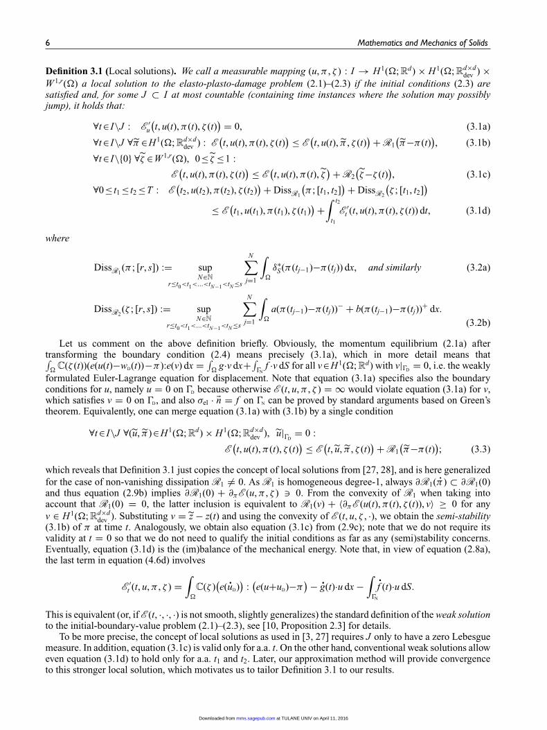
Definition 3.1 (Local solutions). We call a measurable mapping (u, π , ζ ) : I → H1(�; Rd) × H1(�; R

d×ddev ) ×

W 1,r(�) a local solution to the elasto-plasto-damage problem (2.1)–(2.3) if the initial conditions (2.3) aresatisfied and, for some J ⊂ I at most countable (containing time instances where the solution may possiblyjump), it holds that:

∀t∈ I\J : E ′u

(t, u(t), π(t), ζ (t)

) = 0, (3.1a)

∀t∈ I\J ∀π ∈H1(�; Rd×ddev ) : E

(t, u(t), π(t), ζ (t)

) ≤ E(t, u(t), π , ζ (t)

) + R1

(π−π(t)

), (3.1b)

∀t∈ I\{0} ∀ζ ∈W 1,r(�), 0≤ ζ ≤1 :

E(t, u(t), π(t), ζ (t)

) ≤ E(t, u(t), π(t), ζ

) + R2

(ζ−ζ (t)

), (3.1c)

∀0≤ t1 ≤ t2 ≤T : E(t2, u(t2), π(t2), ζ (t2)

) + DissR1

(π ; [t1, t2]

) + DissR2

(ζ ; [t1, t2]

)≤ E

(t1, u(t1), π(t1), ζ (t1)

) +∫ t2

t1

E ′t (t, u(t), π(t), ζ (t)) dt, (3.1d)

where

DissR1(π ; [r, s]) := sup

N∈N

r≤t0<t1<...<tN−1<tN ≤s

N∑j=1

∫�

δ∗S (π(tj−1)−π(tj)) dx, and similarly (3.2a)

DissR2(ζ ; [r, s]) := sup

N∈N

r≤t0<t1<...<tN−1<tN ≤s

N∑j=1

∫�

a(π(tj−1)−π(tj))− + b(π(tj−1)−π(tj))

+ dx.

(3.2b)

Let us comment on the above definition briefly. Obviously, the momentum equilibrium (2.1a) aftertransforming the boundary condition (2.4) means precisely (3.1a), which in more detail means that∫�

C(ζ (t))(e(u(t)−wD(t))−π):e(v) dx = ∫�

g·v dx+∫�N

f ·v dS for all v∈H1(�; Rd) with v|�D

= 0, i.e. the weaklyformulated Euler-Lagrange equation for displacement. Note that equation (3.1a) specifies also the boundaryconditions for u, namely u = 0 on �D because otherwise E (t, u, π , ζ ) = ∞ would violate equation (3.1a) for v,which satisfies v = 0 on �D, and also σel · �n = f on �N can be proved by standard arguments based on Green’stheorem. Equivalently, one can merge equation (3.1a) with (3.1b) by a single condition

∀t∈ I\J ∀(u, π )∈H1(�; Rd) × H1(�; R

d×ddev ), u|�D

= 0 :

E(t, u(t), π(t), ζ (t)

) ≤ E(t, u, π , ζ (t)

) + R1

(π−π(t)

); (3.3)

which reveals that Definition 3.1 just copies the concept of local solutions from [27, 28], and is here generalizedfor the case of non-vanishing dissipation R1 �= 0. As R1 is homogeneous degree-1, always ∂R1(

.π) ⊂ ∂R1(0)

and thus equation (2.9b) implies ∂R1(0) + ∂πE (u, π , ζ ) 0. From the convexity of R1 when taking intoaccount that R1(0) = 0, the latter inclusion is equivalent to R1(v) + 〈∂πE (u(t), π(t), ζ (t)), v〉 ≥ 0 for anyv ∈ H1(�; R

d×ddev ). Substituting v = z − z(t) and using the convexity of E (t, u, ζ , ·), we obtain the semi-stability

(3.1b) of π at time t. Analogously, we obtain also equation (3.1c) from (2.9c); note that we do not require itsvalidity at t = 0 so that we do not need to qualify the initial conditions as far as any (semi)stability concerns.Eventually, equation (3.1d) is the (im)balance of the mechanical energy. Note that, in view of equation (2.8a),the last term in equation (4.6d) involves

E ′t (t, u, π , ζ ) =

∫�

C(ζ )(e(

.uD)

):(e(u+uD)−π

) − .g(t)·u dx −

∫�N

.f (t)·u dS.

This is equivalent (or, if E (t, ·, ·, ·) is not smooth, slightly generalizes) the standard definition of the weak solutionto the initial-boundary-value problem (2.1)–(2.3), see [10, Proposition 2.3] for details.

To be more precise, the concept of local solutions as used in [3, 27] requires J only to have a zero Lebesguemeasure. In addition, equation (3.1c) is valid only for a.a. t. On the other hand, conventional weak solutions alloweven equation (3.1d) to hold only for a.a. t1 and t2. Later, our approximation method will provide convergenceto this stronger local solution, which motivates us to tailor Definition 3.1 to our results.




Actually, local solutions form essentially the largest reasonable class of solutions for rate-independent sys-tems as (2.1)–(2.3) considered here. It includes the mentioned energetic solutions [3, 5], the vanishing-viscositysolutions, the balanced-viscosity (so-called BV) solutions, parametrized solutions (see [3, 4] for a survey), alsostress-driven-like solutions obeying the maximum-dissipation principle in some sense, see Remark 3.2. Theenergetic solutions often have a tendency to undergo damage unphysically early, see [21] for a comparison onseveral computational experiments on a similar type of problem. The approximation method we will use in thisarticle leads rather to the stress-driven option, see Remarks 3.2 and 4.3 below.

Remark 3.2 (Maximum-dissipation principle). The degree-1 homogeneity of R1 and R2 defined in equation(2.8b) allows for further interpretation of the flow rules (2.9b) and (2.9c). Using maximal-monotonicity of thesubdifferential, equation (2.9b) means that 〈ξ − ξplast, v − .

π〉 ≥ 0 for any v and any ξ ∈ ∂R1(v) with the drivingforce ξplast = −E ′

π (t, u, π , ζ ). In particular, for v = 0, defining the convex “elastic domain” K1 = ∂R1(0), oneobtains ⟨

ξplast(t),.π (t)

⟩ = maxξ∈K1

⟨ξ ,

.π (t)

⟩with some ξplast(t) = −E ′

π (t, u(t), π(t), ζ (t)). (3.4a)

To derive it, we have used that ξplast ∈ ∂R1(.π) ⊂ ∂R1(0) = K1 thanks to the degree-0 homogeneity of ∂R1,

so that 〈ξplast,.π〉 ≤ maxξ∈K1

〈ξ ,.π〉. The identity (3.4a) says that the dissipation due to the driving force ξplast

is maximal provided that the order-parameter rate.π is kept fixed, while the vector of possible driving forces

ξ varies freely over all admissible driving force from K1. This just resembles the so-called Hill’s maximum-dissipation principle articulated just for plasticity in [30]. Also it says that the rates are orthogonal to the elasticdomain K1, known as an orthogonality principle [31]. Hill et al. [30] used it for a situation where E (t, ·) is convexwhile, in a general nonconvex case (as also here when damage is considered), it holds only along absolutelycontinuous paths (i.e. in stick or slip regimes) that are sufficiently regular (in the sense that

.π is valued not only

in L1(�; Rd×ddev ) but also in H1(�; R

d×ddev )∗, while it does not need to hold during jumps). Analogously it holds

also for ζ , defining K2 := ∂R2(0), that

⟨ξdam(t),

.ζ (t)

⟩ = maxξ∈K2

⟨ξ ,

.ζ (t)

⟩with some ξdam(t) ∈ −∂ζE (t, u(t), π(t), ζ (t)). (3.4b)

Here, ∂ζE (t, u, π , ζ ) is set-valued and its elements should be understood as “available” driving forces notnecessarily falling into K2, while ξdam ∈ K2 is in a position of an “actual” driving force realized duringthe actual evolution. As E (t, u, ·, ζ ) is smooth, the maximum-dissipation relation (3.4a) written in the form〈−E ′

π (t, u(t), π(t), ζ (t)),.π(t)〉 = max〈K1,

.π(t)〉 = R1(

.π(t)) summed with the semistability (3.1b) which can be

written in the form R1(π ) + 〈E ′π (t, u(t), π(t), ζ (t)), π〉 ≥ 0 thanks to the convexity of E (t, u, ·, ζ ) yields

R1(π) + 〈E ′π (t, u(t), π(t), ζ (t)), π − .

π (t)〉 ≥ R1(.π(t)) (3.5)

for any π , which just means that ξplast(t) = −E ′π (t, u(t), π(t), ζ (t)) ∈ ∂R1(

.π (t)), see equation (2.9b). This means

that the evolution of π is governed by a thermodynamical driving force ξplast (we say that it is “stress-driven”) andit reveals the role of the maximum-dissipation principle in combination with semistability. Using the convexityof E (t, u, π , ·), a similar argument can be applied for equation (3.4b) in combination with semistability (3.1c)even if E (t, u, π , ·) is not smooth.

Remark 3.3 (Integrated maximum-dissipation principle). Let us emphasize that, in general,.π and

.ζ are mea-

sures possibly having singular parts concentrated at times when rupture occurs and the solution and also the

driving forces need not be continuous. Even if.π and

.ζ are absolutely continuous, in our infinite-dimensional

case the driving forces need not be in duality with them, as already mentioned in Remark 3.2. So, equation(3.4) is analytically not justified in any sense. For this reason, an integrated version of the maximum-dissipationprinciple (IMDP) was devised in [10] for a simpler case involving only one maximum-dissipation relation.

Realizing that maxξ∈K1〈ξ ,

.π〉 = R1(

.π) and similarly maxξ∈K2

〈ξ ,.ζ 〉 = R2(

.ζ ), the integrated version of equation




(3.4) reads here as∫ t2

t1

ξplast(t) dπ(t) =∫ t2

t1

R1(.π) dt with ξplast(t) = −E ′

π (t, u(t), π(t), ζ (t)), (3.6a)∫ t2

t1

ξdam(t) dζ (t) =∫ t2

t1

R2(.ζ ) dt with some ξdam(t)∈−∂ζE (t, u(t), π(t), ζ (t)) (3.6b)

to be valid for any 0 ≤ t1 < t2 ≤ T . This definition is inevitably a bit technical and, without sliding into too muchdetail, let us only mention that the left-hand-side integrals in equation (3.6) are the lower Riemann–Stieltjesintegrals which are suitably generalized, and defined by limit superior of lower Darboux sums, i.e.∫ s

rξ (t) dz(t) := lim sup

N∈N

r=t0<t1<...<tN−1<tN =s

N∑j=1

inft∈[tj−1,tj]

⟨ξ (t), z(tj)−z(tj−1)

⟩, (3.7)

relying on the values of ξ being in duality with the values of z (but not necessarily of.z) and on that the collection

of finite partitions of the interval [r, s] forms a directed set when ordered by inclusion so that “limsup” inequation (3.7) is well defined. Let us mention that the conventional definition uses “sup” instead of “limsup”but restricts only to scalar-valued ζ and z with z non-decreasing. The limit-construction (3.7) is called a (herelower) Moore–Pollard–Stieltjes integral [32,33] used here for vector-valued functions in duality, which is a veryspecial case of a so-called multilinear Stieltjes integral. As in the aforementioned classical scalar situation of thelower Riemann–Stieltjes integral using “sup” instead of “limsup”, the sub-additivity of the integral with respectto u and to v holds, in addition to additivity, which holds with respect to the domain.

The right-hand-side integrals in equation (3.6) are just the integrals of measures and equal toDissR1

(π ; [t1, t2]) and DissR2(ζ ; [t1, t2]), respectively. Equivalently, in view of the definition in equation(3.2),

they can be also written as∫ t2

t1R1 dπ(t) and

∫ t2t1

R2 dζ (t), where the integrals can again be understood as thelower Moore–Pollard–Stieltjes integrals (or here as the aforementioned lower Riemann–Stieltjes integrals) mod-ified for the case that the time-dependent linear functionals ξ are replaced by nonlinear but time-constant and1-homogeneous convex functionals R’s. Alternatively, though not equivalently, denoting the internal variablesz = (π , ζ ), the IMDP (3.6) can be written “more compactly” as∫ t2

t1

ξ (t) dz(t) =∫ t2

t1

R dz(t) with some ξ (t)∈−∂zE (t, u(t), z(t)). (3.8)

Both IMDP (3.6) or (3.8) are satisfied on any interval [t1, t2] where the solution to equation (2.9) is abso-lutely continuous with sufficiently regular time derivatives; then the integrals in equation (3.6) are the con-ventional Lebesgue integrals, in particular the left-hand sides in equation (3.6) are

∫ t2t1

〈ξplast(t),.π(t)〉 dt and∫ t2

t1〈ξdam(t),

.ζ (t)〉 dt, respectively. The particular importance of IMDP is especially seen at jumps, i.e. at times

when abrupt damage can happen. It is shown in [4, 10] in various finite-dimensional examples of “damageablesprings” that this IMDP can identify too early, rupturing local solutions when the driving force is obviouslyunphysically low (which occurs in particular within the energetic solutions of systems governed by nonconvexpotentials, as here); its satisfaction for left-continuous local solutions indicates that the evolution is stress driven,as explained in Remark 3.2. On the other hand, it does not need to be satisfied even in physically well justifiedstress-driven local solutions. For example, this happens if two springs with different fracture toughness orga-nized in parallel rupture at the same time, see [4, Example 4.3.40], although even in this situation our algorithm(4.2) below will give a correct approximate solution, see Figure 6. Therefore, even the IMDP (3.6) may serveonly as a sufficient a posteriori condition whose satisfaction verifies the obtained local solution as physicallyrelevant (in the sense that it is stress driven but its dissatisfaction does not mean anything). Eventually, let usrealize that, as a consequence of the mentioned definitions, we have∫ t2

t1

ξplast(t) dπ(t) +∫ t2

t1

ξdam(t) dζ (t) ≤∫ t2

t1

ξ (t) d(π , ζ )(t) and (3.9a)∫ t2

t1

R1 dπ(t) +∫ t2

t1

R2 dζ (t) =∫ t2

t1

(R1+R2

)d(π , ζ )(t). (3.9b)




As there is only inequality in equation (3.9a), the IMDP (3.8) is less selective than (3.6) in general. Moreover,we will rely rather on some approximation of IMDP, see Remarks 4.3 and 6.2.

4. Semi-implicit time discretization and its convergenceTo prove the existence of local solutions, we use a constructive method relying on a suitable time discretiza-tion and the weak compactness of level sets of the minimization problems arising at each time level. Whenfurther discretized in space, it will later in Section 5 yield a computer-implementable efficient algorithm. Let ussummarize the assumption on the data of the original continuous problem

C(·), H ∈ Rd×d×d×d positive definite, symmetric, C : [0, 1] → R

d×d×d×d continuous, (4.1a)

a, b, κ1, κ2 > 0, S ⊂ Rd×ddev convex, bounded, closed, int S 0, (4.1b)

wD ∈ W 1,1(I ; W 1/2,2(�D; Rd)), (4.1c)

g ∈ W 1,1(I ; Lp(�; Rd)) with p

{> 1 for d = 2,= 2d/(d+2) for d ≥ 3 (4.1d)

f ∈ W 1,1(I ; Lp(�N; Rd)) with p

{> 1 for d = 2,= 2−2/d for d ≥ 3, (4.1e)

(u0, π0, ζ0) ∈ H1(�; Rd)×H1(�; R

d×ddev )×W 1,r(�). (4.1f)

The qualification (4.1c) allows for an extension uD of wD which belongs to W 1,1(I ; H1(�; Rd)); in what follows,

we will consider some extension to this property.For the aforementioned time discretization, we use an equidistant partition of the time interval I = [0, T]

with a time step τ > 0, assuming T/τ ∈ N, and denote {ukτ }T/τ

k=0 an approximation of the desired values u(kτ ),and similarly ζ k

τ is to approximate ζ (kτ ), etc.We use a decoupled semi-implicit time discretization with the fractional steps based on the splitting of the

state variables governed by the separately-convex character of E (t, ·, ·, ·). This will make the numerics consid-erably easier than any other splitting and simultaneously may lead to a physically relevant solution governedrather by stresses (if the maximum-dissipation principle holds at least approximately in the sense of Remark 4.3below) than by energies and will prevent too-early debonding (as explained in Section 3). More specifically,

exploiting the convexity of both E (t, ·, ·, ζ ) and E (t, u, π , ·) and the additivity R = R1(.π) + R2(

.ζ ), this split-

ting will be considered as (u, π) and ζ . This yields alternating convex minimization. Thus, for (π k−1τ , ζ k−1

τ )given, we obtain two minimization problems

minimize E kτ (u, π , ζ k−1

τ ) + R1(π−π k−1τ )

subject to (u, π) ∈ H1(�; Rd) × H1(�; R

d×ddev ), u|�D

= 0,

}(4.2a)

with E kτ := E (kτ , ·, ·, ·) and, denoting the unique solution as (uk

τ , π kτ )

minimize E kτ (uk

τ , π kτ , ζ ) + R2(ζ−ζ k−1

τ )subject to ζ ∈ W 1,r(�), 0 ≤ ζ ≤ 1,

}(4.2b)

and denote its (possibly not unique) solution by ζ kτ . Existence of the discrete solutions (uk

τ , π kτ , ζ k

τ ) isstraightforward by the aforementioned compactness arguments.

We define the piecewise-constant interpolants

uτ (t) = ukτ & uτ (t) = uk−1

τ ,πτ (t) = π k

τ & πτ (t) = π k−1τ ,

ζ τ (t) = ζ kτ & ζ

τ(t) = ζ k−1

τ ,

Eτ (t, u, π , ζ ) = E kτ (u, π , ζ )

⎫⎪⎪⎪⎬⎪⎪⎪⎭ for (k−1)τ < t ≤ kτ . (4.3)




Later in Remark 4.3, we will also use the piecewise affine interpolants

πτ (t) = t−(k−1)ττ

π kτ + kτ−t

τπ k−1

τ ,

ζτ (t) = t−(k−1)ττ

ζ kτ + kτ−t

τζ k−1τ

}for (k−1)τ < t ≤ kτ . (4.4)

The important attribute of the discretization (4.2) is also its numerical stability and satisfaction of a suitablediscrete analog of (3.1), namely:

Proposition 4.1 (Stability of the time discretization). Let equation (4.1) hold and, in terms of the interpolants(4.3), (uτ , πτ , ζ τ ) be an approximate solution obtained by equation (4.2). Then, the following a priori estimateshold ∥∥uτ

∥∥L∞(I;H1(�;Rd))

≤ C, (4.5a)∥∥πτ

∥∥L∞(I;H1(�;Rd×d

dev ))∩BV(I;L1(�;Rd×ddev ))

≤ C, (4.5b)∥∥ζ τ

∥∥L∞(�)∩BV(I;L1(�))

≤ C. (4.5c)

Moreover, the obtained approximate solution satisfies for any t ∈ I\{0} the (weakly formulated) Euler-Lagrangeequation for the displacement

E ′u

(tτ , uτ (t), πτ (t), ζ

τ(t)

) = 0, (4.6a)

with tτ := min{kτ ≥ t; k ∈N}, two separate semi-stability conditions for ζ τ and πτ

∀π ∈H1(�; Rd×ddev ) : E

(tτ , uτ (t), πτ (t), ζ

τ(t)

) ≤ E(tτ , uτ (t), π , ζ

τ(t)

) + R1

(π−πτ (t)

), (4.6b)

∀ζ ∈W 1,r(�), 0≤ ζ ≤1 :

E(tτ , uτ (t), πτ (t), ζ τ (t)

) ≤ E(tτ , uτ (t), πτ (t), ζ

) + R2

(ζ−ζ τ (t)

), (4.6c)

and, for all 0 ≤ t1 < t2 ≤ T of the form ti = kiτ for some ki ∈N, the energy (im)balance

E(t2, uτ (t2), πτ (t2), ζ τ (t2)

) + DissR1

(πτ ; [t1, t2]

) + DissR2

(ζ τ ; [t1, t2]

)≤ E

(t1, uτ (t1), πτ (t1), ζ τ (t1)

) +∫ t2

t1

E ′t

(t, uτ (t), π (t), ζ (t)) dt. (4.6d)

Sketch of the proof. Writing the optimality condition for equation (4.2a) in terms of u, one arrives at equation(4.6a), and by comparing the value of equation (4.2a) at (uk

τ , π kτ ) with its value at (uk

τ , π ) and using the degree-1homogeneity of R1, one arrives at equation (4.6b).

By comparing the value of equation (4.2b) at ζ kτ with its value at ζ and using the degree-1 homogeneity of

R2, one arrives at equation (4.6c).In obtaining equation (4.6d), we compare the value of equation (4.2a) at the minimizer (uk

τ , π kτ ) with the

value at (uk−1τ , π k−1

τ ), and also the value of equation (4.2b) at the minimizer ζ kτ with the value at ζ k−1

τ . Webenefit from the cancellation of the terms ±E (kτ , uk

τ , π kτ , ζ k−1

τ ). We also use the discrete by-part integration(= summation) for the E ′

t -term.Then, using equation (4.6d) for t1 = 0 and the coercivity of E (t, ·, ·, ·) due to the assumptions (4.1), we

obtain also the a priori estimates (4.5). �The cancellation effect mentioned in the above proof is typical in fractional-step methods, see for example

[34, Remark 8.25]. Further, note that equation (4.6) is of a similar form as equation (3.1) and is thus preparedto make a limit passage for τ → 0:

Proposition 4.2 (Convergence towards local solutions). Let (4.1) hold and let (uτ , πτ , ζ τ ) be an approximatesolution obtained by the semi-implicit formula (4.2). Then there exists a subsequence (indexed again by τ for




notational simplicity) and u ∈ B([0, T]; H1(�; Rd)) and π ∈ B([0, T]; H1(�; R

d×ddev )) ∩ BV([0, T]; L1(�; R

d×ddev ))

and ζ ∈ B([0, T]; W 1,r(�)) ∩ BV([0, T]; L1(�)) such that

uτ (t) → u(t) in H1(�; Rd) for all t ∈ [0, T], (4.7a)

πτ (t) → π(t) in H1(�; Rd×ddev ) for all t ∈ [0, T], (4.7b)

ζ τ (t) → ζ (t) in W 1,r(�) for all t ∈ [0, T]. (4.7c)

Moreover, any (u, π , ζ ) obtained by this way is a local solution to the damage/plasticity problem in the sense ofDefinition 3.1.

Proof. By a (generalized) Helly’s selection principle, see [3, 4], we choose a subsequence and π ∈B([0, T]; H1(�; R

d×ddev )) ∩ BV([0, T]; L1(�; R

d×ddev )) and ζ , ζ∗ ∈ B([0, T]; W 1,r(�)) ∩ BV([0, T]; L1(�)) so that

πτ (t) ⇀ π(t) in H1(�; Rd×ddev ) for all t∈ [0, T], (4.8a)

ζ τ (t) ⇀ ζ (t) & ζτ(t) ⇀ ζ∗(t) in W 1,r(�) for all t∈ [0, T]. (4.8b)

Now, for a fixed t ∈ [0, T], by Banach’s selection principle, we select (for a moment) a further subsequence sothat

uτ (t) ⇀ u(t) in H1(�; Rd). (4.9)

We further use that uτ (t) minimizes E (tτ , ·, πτ (t), ζτ(t)) with tτ := min{kτ ≥ t; k ∈ N}. Obviously, tτ → t

for τ → 0 and, by the weak-lower-semicontinuity argument, we can easily see that u(t) minimizes the strictlyconvex functional E (t, ·, ζ∗(t), π(t)); this is indeed simple to prove due to the compactness in both π and ζdue to the gradient theories involved. Thus u(t) is determined uniquely so that, in fact, we did not need tomake further selection of a subsequence, and this procedure can be performed for any t by using the samesubsequence already selected for equation (4.8). Also, u : [0, T] → H1(�; R

d) is measurable because π and ζ∗are measurable, and E ′

u(t, u(t), π(t), ζ∗(t))=0 for all t.The key ingredient is improvement of the weak convergence (4.8) and (4.9) for the strong convergence. For

the strong convergence in u and π , we use the uniform convexity of the quadratic form induced by C(ζ ), H, andκ1 with the information we have at disposal from (4.6b) leading, when using the abbreviation eel = e(u−uD)−πand eel,τ = e(uτ−uD,τ ) − πτ , to the estimate∫

�

C(ζτ(t))

(eel,τ (t)−eel(t)

):(eel,τ (t)−eel(t)

)+ H

(πτ (t)−π(t)

):(πτ (t)−π(t)

) + κ1

2

∣∣∇πτ (t)−∇π(t)∣∣2

dx

≤∫

�

−C(ζτ(t))eel(t) :

(eel,τ (t)−eel(t)

) − (Hπ(t)−ξ τ (t)

):(πτ (t)−π(t)

)+ κ1

2∇π(t) : ∇(

πτ (t)−π(t)) − f τ (t)·(uτ (t)−u(t)) dx −

∫�N

gτ (t)·(uτ (t)−u(t)) dS → 0

where we use some ξ τ (t) ∈ ∂δ∗S (πτ (t)) which solves at time t in the weak sense the discrete plastic flow-rule

ξ τ + Hπτ − dev σ τ = κ1�πτ with σ τ = C(ζτ)eel,τ . Thus we proved

eel,τ (t) → eel(t) strongly in L2(�; Rd×dsym )

together with equation (4.7b). Realizing that e(uτ (t)) = e(uD,τ (t)) + πτ (t) + eel,τ (t), we obtain also e(uτ (t)) →e(u(t)) strongly in L2(�; R

d×dsym ), and thus also (4.7a). Note that we exploited the gradient theory for plasticity

which ensures that the sequence (ξ τ )τ>0, which is bounded in L∞(�; Rd×ddev ) because the plastic domain S ⊂

Rd×ddev is bounded, is relatively compact in H1(�; R

d×ddev )∗ so that the term

∫�

ξτ (t) : (πτ (t)−π(t)) dx indeedconverges to zero because πτ (t) ⇀ π(t) in H1(�; R

d×ddev ).




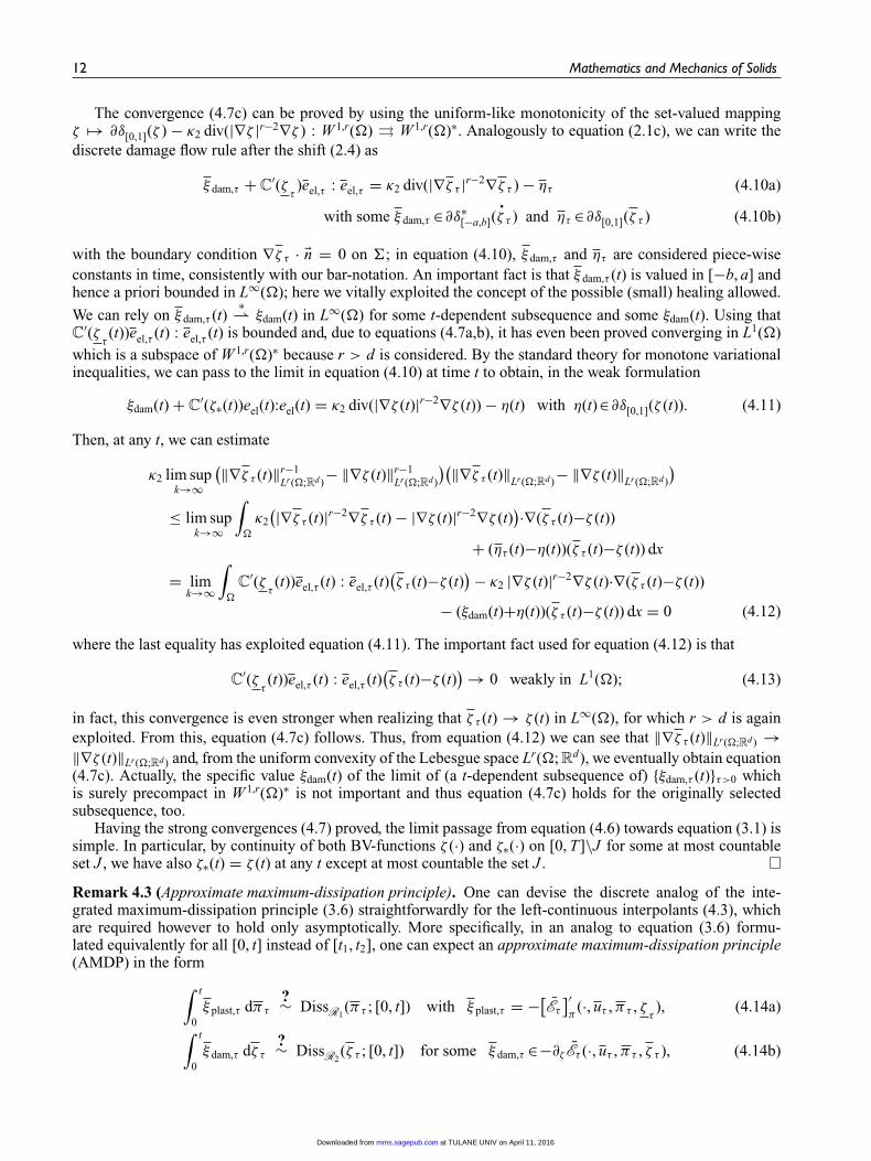
The convergence (4.7c) can be proved by using the uniform-like monotonicity of the set-valued mappingζ �→ ∂δ[0,1](ζ ) − κ2 div(|∇ζ |r−2∇ζ ) : W 1,r(�) ⇒ W 1,r(�)∗. Analogously to equation (2.1c), we can write thediscrete damage flow rule after the shift (2.4) as

ξ dam,τ + C′(ζ

τ)eel,τ : eel,τ = κ2 div(|∇ζ τ |r−2∇ζ τ ) − ητ (4.10a)

with some ξ dam,τ ∈∂δ∗[−a,b](

.ζ τ ) and ητ ∈∂δ[0,1](ζ τ ) (4.10b)

with the boundary condition ∇ζ τ · �n = 0 on �; in equation (4.10), ξ dam,τ and ητ are considered piece-wiseconstants in time, consistently with our bar-notation. An important fact is that ξ dam,τ (t) is valued in [−b, a] andhence a priori bounded in L∞(�); here we vitally exploited the concept of the possible (small) healing allowed.

We can rely on ξ dam,τ (t)∗

⇀ ξdam(t) in L∞(�) for some t-dependent subsequence and some ξdam(t). Using thatC

′(ζτ(t))eel,τ (t) : eel,τ (t) is bounded and, due to equations (4.7a,b), it has even been proved converging in L1(�)

which is a subspace of W 1,r(�)∗ because r > d is considered. By the standard theory for monotone variationalinequalities, we can pass to the limit in equation (4.10) at time t to obtain, in the weak formulation

ξdam(t) + C′(ζ∗(t))eel(t):eel(t) = κ2 div(|∇ζ (t)|r−2∇ζ (t)) − η(t) with η(t)∈∂δ[0,1](ζ (t)). (4.11)

Then, at any t, we can estimate

κ2 lim supk→∞

(‖∇ζ τ (t)‖r−1Lr(�;Rd)

− ‖∇ζ (t)‖r−1Lr(�;Rd)

)(‖∇ζ τ (t)‖Lr(�;Rd)− ‖∇ζ (t)‖Lr(�;Rd)

)≤ lim sup

k→∞

∫�

κ2

(|∇ζ τ (t)|r−2∇ζ τ (t) − |∇ζ (t)|r−2∇ζ (t))·∇(ζ τ (t)−ζ (t))

+ (ητ (t)−η(t))(ζ τ (t)−ζ (t)) dx

= limk→∞

∫�

C′(ζ

τ(t))eel,τ (t) : eel,τ (t)

(ζ τ (t)−ζ (t)

) − κ2 |∇ζ (t)|r−2∇ζ (t)·∇(ζ τ (t)−ζ (t))

− (ξdam(t)+η(t))(ζ τ (t)−ζ (t)) dx = 0 (4.12)

where the last equality has exploited equation (4.11). The important fact used for equation (4.12) is that

C′(ζ

τ(t))eel,τ (t) : eel,τ (t)

(ζ τ (t)−ζ (t)

) → 0 weakly in L1(�); (4.13)

in fact, this convergence is even stronger when realizing that ζ τ (t) → ζ (t) in L∞(�), for which r > d is againexploited. From this, equation (4.7c) follows. Thus, from equation (4.12) we can see that ‖∇ζ τ (t)‖Lr(�;Rd) →‖∇ζ (t)‖Lr(�;Rd) and, from the uniform convexity of the Lebesgue space Lr(�; R

d), we eventually obtain equation(4.7c). Actually, the specific value ξdam(t) of the limit of (a t-dependent subsequence of) {ξdam,τ (t)}τ>0 whichis surely precompact in W 1,r(�)∗ is not important and thus equation (4.7c) holds for the originally selectedsubsequence, too.

Having the strong convergences (4.7) proved, the limit passage from equation (4.6) towards equation (3.1) issimple. In particular, by continuity of both BV-functions ζ (·) and ζ∗(·) on [0, T]\J for some at most countableset J , we have also ζ∗(t) = ζ (t) at any t except at most countable the set J .

Remark 4.3 (Approximate maximum-dissipation principle). One can devise the discrete analog of the inte-grated maximum-dissipation principle (3.6) straightforwardly for the left-continuous interpolants (4.3), whichare required however to hold only asymptotically. More specifically, in an analog to equation (3.6) formu-lated equivalently for all [0, t] instead of [t1, t2], one can expect an approximate maximum-dissipation principle(AMDP) in the form∫ t

0ξ plast,τ dπτ

?∼ DissR1(πτ ; [0, t]) with ξ plast,τ = −[

Eτ

]′π

(·, uτ , πτ , ζτ), (4.14a)∫ t

0ξ dam,τ dζ τ

?∼ DissR2(ζ τ ; [0, t]) for some ξ dam,τ ∈−∂ζ Eτ (·, uτ , πτ , ζ τ ), (4.14b)




or, analogously to equation (3.8)∫ t

0ξ τ dzτ

?∼ DissR(zτ ; [0, t]) with some ξ τ ∈ {−[Eτ

]′π

(·, uτ , πτ , ζτ)} × −∂ζ Eτ (·, uτ , πτ , ζ τ ), (4.15)

where the integrals are again the lower Moore–Pollard–Stieltjes integrals as in equation (3.6) and whereEτ (·, u, π , ζ ) is the left-continuous piecewise-constant interpolant of the values E (kτ , u, π , ζ ), k = 0, 1, ..., T/τ .

Moreover, ”?∼” in equation (4.14) means that the equality holds possibly only asymptotically for τ → 0, but

even this is only desirable and not always valid. Loadings which, under the given geometry of the specimen, leadto rate-independent slides where the solution is absolutely continuous will always comply with AMDP (4.14).Also, some finite-dimensional examples of “damageable springs” in [4, 10] show that this AMDP can detectrupturing local solutions too early (in particular the energetic ones), while it generically holds for solutionsobtained by the algorithm (4.2). Generally speaking, equation (4.14) should be checked a posteriori to justifythe (otherwise not physically based) simple and numerically efficient fractional-step-type semi-implicit algo-rithm (4.2) from the perspective of the stress-driven solutions in particular situations, and possibly to providevaluable information that can be exploited to adapt time or space discretization towards better accuracy in equa-tion (4.14) (and thus close towards the stress-driven scenario). Actually, for the piecewise-constant interpolants,we can simply evaluate the integrals explicitly, so that AMDP (4.15) reads

K∑k=1

∫�

δ∗S (π(tj−1)−π(tj)) + a

(ζ kτ −ζ k−1

τ

)−+ b(ζ kτ −ζ k−1

τ

)+dx⟨

ξ k−1plast,τ , π k

τ −π k−1τ

⟩ − ⟨ξ k−1

dam,τ , ζ kτ −ζ k−1

τ

⟩ =: ετ

?↘ 0 (4.16)

where ξ kplast,τ = −[

E kτ

]′π

(ukτ , π k

τ , ζ k−1τ ) and ξ k

dam,τ ∈ −∂ζEkτ (uk

τ , π kτ , ζ k

τ )

where K = max{k ∈ N; kτ ≤ t} and the notation “?↘ ” means that it is only a desired but not granted

convergence. Notably, in contrast to equations (3.6) and (3.8), the AMDP (4.14) and (4.15) are equivalent toeach other as the limsup’s (see definition (3.7)) in all involved integrals is attained on the equidistant partitionswith the time step τ , and the “inf” in the Darboux sums is redundant. Evaluating the dualities, the residuum ετ

in equation (4.16) can be written more explicitly as ετ = ∫�

RKτ dx ≥ 0 with the local residuum

RKτ :=

K∑k=1

(δ∗

S (π(tj−1)−π(tj)) + a(ζ kτ −ζ k−1

τ

)−+ b(ζ kτ −ζ k−1

τ

)+

−(C(ζ k−2

τ )(π k−1

τ − e(uk−1τ +uk−1

D,τ )) + Hπ k−1

τ

):(π k

τ −π k−1τ

)−

(1

2C

′(ζ k−1τ )

(e(uk−1

τ +uk−1D,τ )−π k−1

τ

):(e(uk−1

τ +uk−1D,τ )−π k−1

τ

) + ξ k−1const,τ

)(ζ kτ −ζ k−1

τ

)− κ1∇π k−1

τ

... ∇(π k

τ −π k−1τ

) − κ2

∣∣∇ζ k−1τ

∣∣r−2∇ζ k−1τ ·∇(

ζ kτ −ζ k−1

τ

))(4.17)

with some multiplier ξ kconst,τ ∈N[0,1](ζ

kτ ) and with ζ k−2

τ for k = 1 equal to ζ0. Note that RKτ cannot be guaranteed

to be non-negative pointwise on �, only their integrals over � are non-negative. One can check the residua aposteriori depending on t or possibly also on space, see also [12, 21] for a surface variant of such a model orFigures 4–7 below.

5. Implementation of the discrete modelTo implement the model computationally, we need to make a spatial discretization of the variables from thesemi-implicit time discretization of Section 4. Essentially, we apply conformal Galerkin (also called Ritz)method to the minimization problems (4.2a) and (4.2b) which are then restricted to the corresponding finite-dimensional subspaces. These subspaces are constructed by the finite-element method (FEM), and the solutionthus obtained is denoted by

qkτh := (

ukτh, π k

τh, ζ kτh

),




with h > 0 denoting the mesh size of the triangulation, let us denote it by Th, of the domain � consideredpolyhedral here; later in Section 6 we consider d = 2 and henceforth a polyhedral domain. In this way, weobtain also the piecewise constant and the piecewise affine interpolants in time, denoted respectively by uτh

and uτh, πτh and πτh, and eventually ζ τh and ζτh. The simplest option is to consider the lowest-order conformalFEM, i.e. P1-elements for u, ζ , and π . In Section 6, only the case d = 2 will be treated, so the previous analyticalparts have required r > 2 and we make an (indeed small) shortcut by considering r = 2. Moreover, we will notconsider the loading on �N, so f = 0.

The material is assumed to be isotropic with properties linearly dependent on damage. The isotropicelasticity tensor is assumed to be

Cijkl(ζ ) := [(λ1−λ0)ζ + λ0

]δijδkl + [

(μ1−μ0)ζ + μ0

](δikδjl+δilδjk

)(5.1)

where λ1, μ1 and λ0, μ0 are two sets of Lamé parameters satisfying λ1 ≥ λ0 ≥ 0 and μ1 ≥ μ0 > 0. Here, δdenotes the Kronecker symbol. This choice implies that the elastic-moduli tensor is positively-definite-valued(and therefore is invertible). The elastic domain S is assumed to satisfy

S = {σ ∈ R

d×ddev ; |σ | ≤ σ

Y

}, (5.2)

where σY

> 0 is a given plastic yield stress. More specifically, the minimization problems (4.2) after spatialdiscretization can be rewritten as

(ukτh, π k

τh) = argminu∈W1,∞(�;Rd)

π∈W1,∞(�;Rd×ddev )

u,π elementwise affine on Th

∫�

(1

2C(ζ k−1

τh )(e(u+uk

D,τh)−π)

:(e(u+uk

D,τh)−π)

+ 1

2Hπ :π + κ1

2|∇π |2− gk

τh·u + σY|π−π k−1

τh |)

dx, (5.3a)

ζ kτh = argmin

ζ∈W1,∞(�)0≤ζ≤1 on �

ζ elementwise affine on Th

∫�

(1

2C(ζ )

(e(uk

τh+ukD,τh)−π k

τh

):(e(uk

τh+ukD,τh)−π k

τh

)+ κ2

2|∇ζ |2+ a(ζ−ζ k−1

τh )− + b(ζ−ζ k−1τh )+

)dx. (5.3b)

The damage problem (5.3b) represents a minimization of a nonsmooth but strictly convex functional. Tofacilitate its numerical solution, we still modify it a bit, namely

argminζ , ζ� , ζ�∈W1,∞(�)

0≤ζ≤1 on �

ζ ,ζ� ,ζ� elementwise affine on Th

∫�

(1

2C(ζ )

(e(uk

τh+ukD,τh)−π k

τh

):(e(uk

τh+ukD,τh)−π k

τh

)+ κ2

2|∇ζ |2 + aζ� + bζ�

)dx, (5.4a)

where ζ� = (ζ−ζ k−1τh )+ and ζ� = (ζ−ζ k−1

τh )− at all nodal points. (5.4b)

We used additional auxiliary ‘update’ variables ζ� and ζ� which are also considered as P1-functions. This mod-ification can also be understood as a certain specific numerical integration applied to the original minimizationproblem (5.3b). It should be noted that ζ and ζ k−1

τh are P1-functions and, if we would require equation (5.4b)to be valid everywhere on �, ζ� and ζ� could not be P1-functions in general on elements where nodal valuesof ζ−ζ k−1

τh alternate signs. The important advantage of equation (5.4b) required only at nodal points (while atremaining points it is fulfilled only approximately (depending on h)) is that equation (5.4a) actually representsa conventional quadratic-programming problem (QP) involving the linear and the box constraints

ζ = ζ k−1τh + ζ� − ζ�, 0 ≤ ζ� ≤ 1 − ζ k−1

τh , 0 ≤ ζ� ≤ ζ k−1τh . (5.5)

A convex quadratic cost functional of this QP problem has only a positive-semidefinite Jacobian, since thereare no Dirichlet boundary conditions on the damage variable ζ . Note that the optimal pair (ζ�, ζ�) must satisfyζ�ζ�=0 in all nodes, i.e. both variables cannot be positive. This can be easily seen by contradiction: If ζ�ζ�>0in some node, then a different pair (ζ�− min{ζ�, ζ�}, ζ�− min{ζ�, ζ�}) would again satisfy the constraints(5.5) but would provide a smaller energy value in (5.4a).




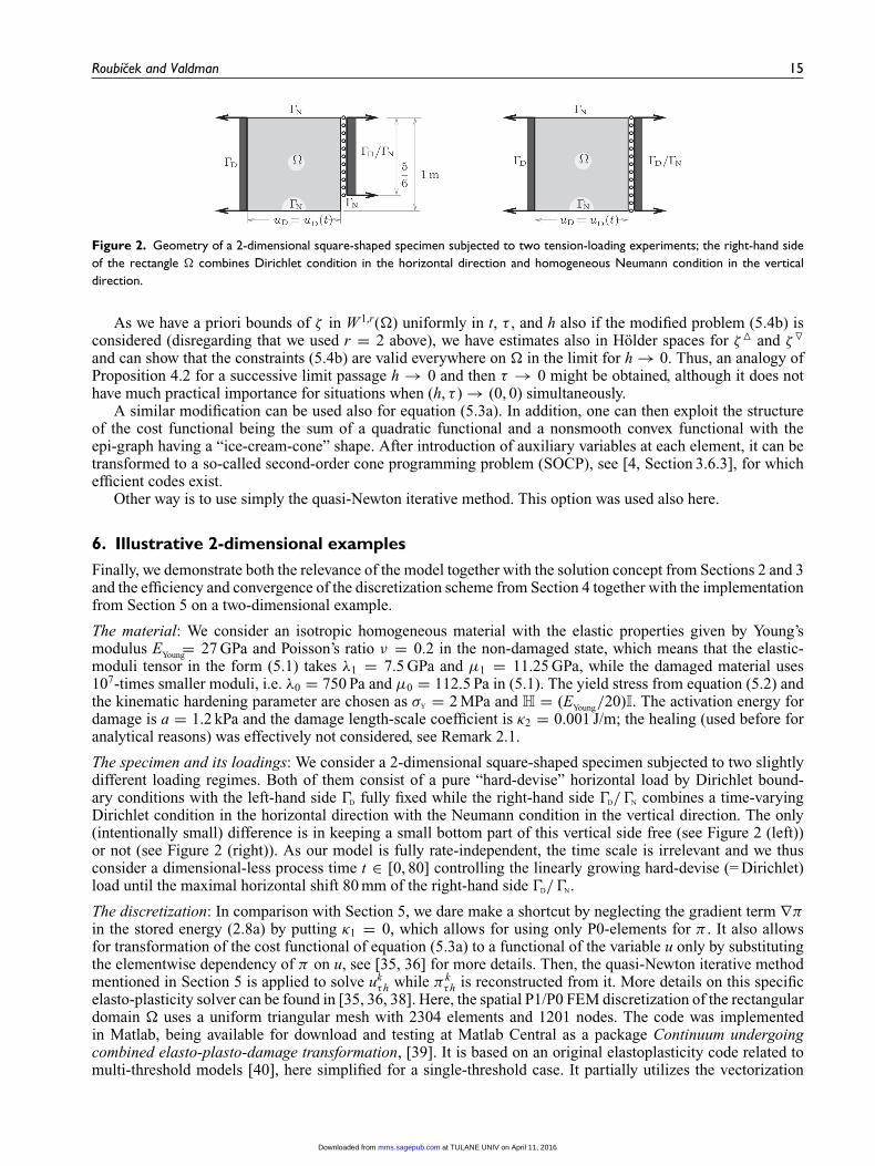
Figure 2. Geometry of a 2-dimensional square-shaped specimen subjected to two tension-loading experiments; the right-hand sideof the rectangle � combines Dirichlet condition in the horizontal direction and homogeneous Neumann condition in the verticaldirection.

As we have a priori bounds of ζ in W 1,r(�) uniformly in t, τ , and h also if the modified problem (5.4b) isconsidered (disregarding that we used r = 2 above), we have estimates also in Hölder spaces for ζ� and ζ�and can show that the constraints (5.4b) are valid everywhere on � in the limit for h → 0. Thus, an analogy ofProposition 4.2 for a successive limit passage h → 0 and then τ → 0 might be obtained, although it does nothave much practical importance for situations when (h, τ ) → (0, 0) simultaneously.

A similar modification can be used also for equation (5.3a). In addition, one can then exploit the structureof the cost functional being the sum of a quadratic functional and a nonsmooth convex functional with theepi-graph having a “ice-cream-cone” shape. After introduction of auxiliary variables at each element, it can betransformed to a so-called second-order cone programming problem (SOCP), see [4, Section 3.6.3], for whichefficient codes exist.

Other way is to use simply the quasi-Newton iterative method. This option was used also here.

6. Illustrative 2-dimensional examplesFinally, we demonstrate both the relevance of the model together with the solution concept from Sections 2 and 3and the efficiency and convergence of the discretization scheme from Section 4 together with the implementationfrom Section 5 on a two-dimensional example.

The material: We consider an isotropic homogeneous material with the elastic properties given by Young’smodulus EYoung= 27 GPa and Poisson’s ratio ν = 0.2 in the non-damaged state, which means that the elastic-moduli tensor in the form (5.1) takes λ1 = 7.5 GPa and μ1 = 11.25 GPa, while the damaged material uses107-times smaller moduli, i.e. λ0 = 750 Pa and μ0 = 112.5 Pa in (5.1). The yield stress from equation (5.2) andthe kinematic hardening parameter are chosen as σY = 2 MPa and H = (EYoung/20)I. The activation energy fordamage is a = 1.2 kPa and the damage length-scale coefficient is κ2 = 0.001 J/m; the healing (used before foranalytical reasons) was effectively not considered, see Remark 2.1.

The specimen and its loadings: We consider a 2-dimensional square-shaped specimen subjected to two slightlydifferent loading regimes. Both of them consist of a pure “hard-devise” horizontal load by Dirichlet bound-ary conditions with the left-hand side �D fully fixed while the right-hand side �D/�N combines a time-varyingDirichlet condition in the horizontal direction with the Neumann condition in the vertical direction. The only(intentionally small) difference is in keeping a small bottom part of this vertical side free (see Figure 2 (left))or not (see Figure 2 (right)). As our model is fully rate-independent, the time scale is irrelevant and we thusconsider a dimensional-less process time t ∈ [0, 80] controlling the linearly growing hard-devise (= Dirichlet)load until the maximal horizontal shift 80 mm of the right-hand side �D/�N.

The discretization: In comparison with Section 5, we dare make a shortcut by neglecting the gradient term ∇πin the stored energy (2.8a) by putting κ1 = 0, which allows for using only P0-elements for π . It also allowsfor transformation of the cost functional of equation (5.3a) to a functional of the variable u only by substitutingthe elementwise dependency of π on u, see [35, 36] for more details. Then, the quasi-Newton iterative methodmentioned in Section 5 is applied to solve uk

τh while π kτh is reconstructed from it. More details on this specific

elasto-plasticity solver can be found in [35, 36, 38]. Here, the spatial P1/P0 FEM discretization of the rectangulardomain � uses a uniform triangular mesh with 2304 elements and 1201 nodes. The code was implementedin Matlab, being available for download and testing at Matlab Central as a package Continuum undergoingcombined elasto-plasto-damage transformation, [39]. It is based on an original elastoplasticity code related tomulti-threshold models [40], here simplified for a single-threshold case. It partially utilizes the vectorization




Figure 3. Evolution of averaged elastic von Mises stresses∫� | dev σel| dx over time for the two experiments from Figure 2 for three

different time discretizations. The left experiment ruptures earlier under less stretch and leaving less plastification and remainingstress comparing to the right experiment. In both experiments, the convergence theoretically supported by Proposition 4.2 is welldocumented.

techniques of [41] and works reasonably fast also for finer triangular meshes. In contrast to the fixed spatialdiscretization, we consider three time discretization to document the convergence (theoretically stated only forunspecified subsequences in Proposition 4.2) on particular computational experiments. More specifically, weused three time steps τ = 1, 0.1, or 0.01, i.e. the equidistant partition of the time interval [0, 80] to 80, 800, or8000 time steps, respectively.

Simulation results: The averaged stress/strain (or rather force/stretch) response is depicted in Figure 3. Notably,after damage is completed, some stress still remains (as is nearly independent on further stretch because theelastic moduli λ0 and μ0 are considered very small). These remaining stresses are caused by non-uniformplastification of the specimen during the previous phases of the loading. One can also note that Figure 3 (right)imitates quite well the scenario from Figure 1 (right) while Figure 3 (left) is rather a mixture of both regimesfrom Figure 1 and, interestingly, the rupture proceeds in three stages. The respective spacial distribution ofthe evolving state variable is depicted at few selected instants on Figures 4 and 5. It is seen how a relativelysmall variation of geometry in Figure 2 dramatically changes the spatial scenario and triggers damage in verydifferent spots of the specimen. This is an expected notch-effect causing stress concentration and relativelyearly initiation of cracks at such spots, i.e. here such a notch is the point of the transition �N to �D/�N in Figure 2(left). The AMDP suggested in Remark 4.3 is depicted in Figures 6 and 7. It should be emphasized that themaximum-dissipation principle (as devised originally by Hill [30]) is reliably satisfied only for convex storedenergies as occurs during a mere plastification phase, as also seen in Figure 7. In general it does not need tobe satisfied even in obviously physically relevant stress-driven evolutions, as already mentioned in Remark 3.3,and which can be expected even here during massive fast rupture of a wider region (in spite of this, Figure 6shows a good satisfaction of AMDP even during such rupture phases and in some sense demonstrates a goodapplicability of the model and solution concept and its algorithmic realization).

Remark 6.1 (Symmetry issue). Actually, one could understand the square 1 × 1 in Figure 2 as one half of arectangle with sides 2 × 1, with the right-hand side of the 1 × 1 square being the symmetry axis of the 2 × 1rectangle, which is then loaded from the vertical sides fully symmetrically. Engineers actually routinely assumethat a symmetry of this geometry would be inherited by all (or at least by one) solution(s), and therefore woulduse the reduced geometries on Figure 2 for calculations of the full 2 × 1-rectangle. We intentionally did not usethis interpretation because, in fact, one can only say that the set of all solutions inherits the (possible) symmetryof the specimen and its loading but not particular solutions. It may be that there is no solution inheriting thissymmetry or that experimental evidence shows preferences for nonsymmetric solutions, see the discussion in[42, 43]. In addition, the geometry in Figure 2 (left) would lead to a 2 × 1 rectangle with a partial “cut” in themid-bottom side, which is not a Lipschitz domain.




Figure 4. Evolution of the spatial distribution of the state (u, π , ζ ) with the von Mises stress and the residuum R from equation (4.17)at (equidistantly) selected instants for the asymmetric geometry from Figure 2 (left). The deformation is visualized by a displacementu magnified by 250 ×, with τ = 0.1 used. Damage occurs relatively early on in the right-hand side due to the stress concentration,and propagates in several partial steps, see Figure 3 (left).

Remark 6.2 (Recovery of the integrated maximum-dissipation principle IMDP). It should be emphasized that,even if the intuitively straightforward AMDP is asymptotically satisfied, the recovery of even the less-selectiveIMDP (3.8) for τ → 0 is not clear. This is obviously related to the instability of IMDP under data perturbationif E (t, ·) is not convex. Here, to recover the IMDP on I , it would suffice to show that for all ε > 0 there is τε > 0such that for any 0 < τ ≤ τε it holds

T/τ∑k=1

inft∈[kτ−τ ,kτ ]

⟨ξ (t), z(kτ )−z(kτ−τ )

⟩ − R(z(kτ )−z(kτ−τ )

) ≥ −ε (6.1)

for some selection ξ (t) ∈ −∂zE (t, u(t), z(t)), see definition (3.7). The equi-distant partitions are cofinal in allpartitions of I . This can be guaranteed only under rather strong conditions, namely if, for all ε > 0, there is




Figure 5. Evolution of spatial distribution of the state (u, π , ζ ) with the von Mises stress and the residuum R from equation (4.17)at selected instants for the symmetric geometry from Figure 2 (right). The deformation is visualized by a displacement u magnifiedby 250 ×, where τ = 0.1 was used. The process inherits the symmetry of the specimen and loading. In contrast to Figure 4, damageoccurs rather later on in the left-bottom corner and propagates quickly, hence the snapshots are not selected in an equidistant wayhere.

τε > 0 such that for any 0 < τ ≤ τε, the following strengthened version of the AMDP

T/τε∑k=1

R(zτ (tk) − zτ (tk−1)

) − ⟨ξ τ (t), zτ (tk) − zτ (tk−1)

⟩ ≤ ε (6.2)




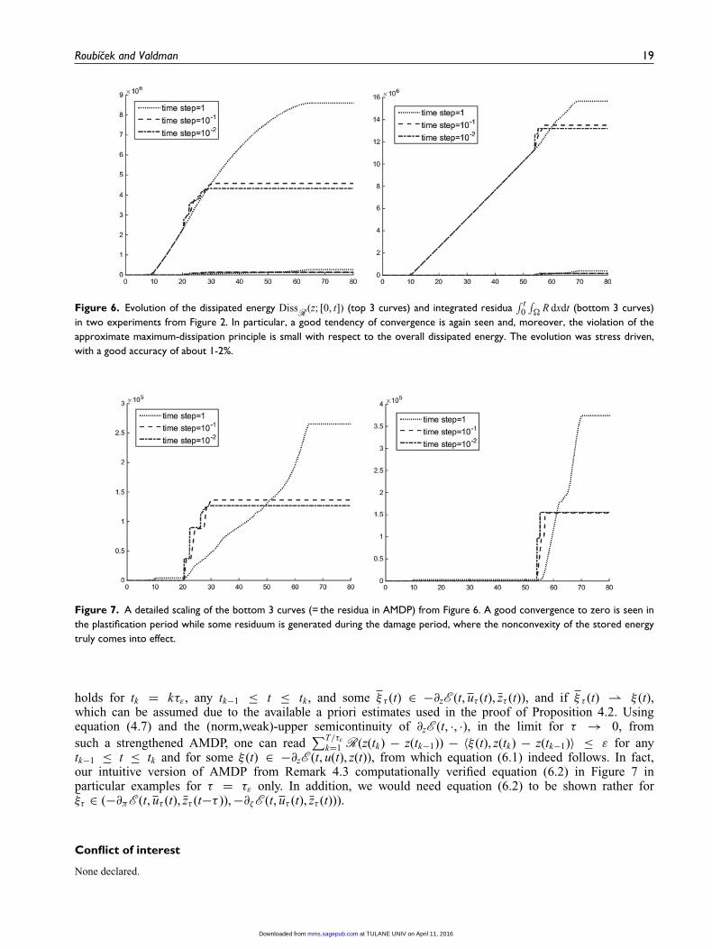
Figure 6. Evolution of the dissipated energy DissR (z; [0, t]) (top 3 curves) and integrated residua∫ t

0∫� R dxdt (bottom 3 curves)

in two experiments from Figure 2. In particular, a good tendency of convergence is again seen and, moreover, the violation of theapproximate maximum-dissipation principle is small with respect to the overall dissipated energy. The evolution was stress driven,with a good accuracy of about 1-2%.

Figure 7. A detailed scaling of the bottom 3 curves (= the residua in AMDP) from Figure 6. A good convergence to zero is seen inthe plastification period while some residuum is generated during the damage period, where the nonconvexity of the stored energytruly comes into effect.

holds for tk = kτε, any tk−1 ≤ t ≤ tk , and some ξ τ (t) ∈ −∂zE (t, uτ (t), zτ (t)), and if ξ τ (t) ⇀ ξ (t),which can be assumed due to the available a priori estimates used in the proof of Proposition 4.2. Usingequation (4.7) and the (norm,weak)-upper semicontinuity of ∂zE (t, ·, ·), in the limit for τ → 0, fromsuch a strengthened AMDP, one can read

∑T/τε

k=1 R(z(tk) − z(tk−1)) − 〈ξ (t), z(tk) − z(tk−1)〉 ≤ ε for anytk−1 ≤ t ≤ tk and for some ξ (t) ∈ −∂zE (t, u(t), z(t)), from which equation (6.1) indeed follows. In fact,our intuitive version of AMDP from Remark 4.3 computationally verified equation (6.2) in Figure 7 inparticular examples for τ = τε only. In addition, we would need equation (6.2) to be shown rather forξτ ∈ (−∂πE (t, uτ (t), zτ (t−τ )), −∂ζE (t, uτ (t), zτ (t))).

Conflict of interest

None declared.




Funding

The author(s) disclosed receipt of the following financial support for the research, authorship, and/or publication of this article: Thisresearch has been supported by GA CR through the projects 13-18652S “Computational modeling of damage and transport processesin quasi-brittle materials” and 14-15264S “Experimentally justified multiscale modelling of shape memory alloys” with also the alsoinstitutional support RVO:61388998 (CR).

References

[1] Han, W and Reddy, BD. Plasticity (Mathematical Theory and Numerical Analysis). New York: Springer-Verlag, 1999.[2] Frémond, M. Non-Smooth Thermomechanics. Berlin: Springer-Verlag, 2002.[3] Mielke, A. Differential, energetic, and metric formulations for rate-independent processes. In: Ambrosio, L, and Savaré, G (eds)

Nonlinear PDEs and Applications (CIME Summer School, Cetraro, Italy 2008, Lecture Notes Math. Volume 2028). Heidelberg:Springer, 2011, 87–170.

[4] Mielke, A, and Roubícek, T. Rate Independent Systems - Theory and Application. New York: Springer, 2015.[5] Mielke, A, and Theil, F. On rate-independent hysteresis models. NoDEA-Nonlinear Diff 2004; 11: 151–189.[6] Alessi, R, Marigo, JJ, and Vidoli, S. Gradient damage models coupled with plasticity and nucleation of cohesive cracks. Arch

Ration Mech An 2014; 214: 575–615.[7] Alessi, R, Marigo, JJ, and Vidoli, S. Gradient damage models coupled with plasticity: Variational formulation and main

properties. Mech Mater 2015; 80 B: 351–367.[8] Crismale, V. Globally stable quasistatic evolution for a coupled elastoplastic-damage model. ESAIM: Control Optim Calc Var,

2014. DOI: 10.1051/cocv/2015037.[9] Leguillon, D. Strength or toughness? A criterion for crack onset at a notch. Eur J Mech A-Solid 2002; 21: 61–72.[10] Roubícek, T. Maximally-dissipative local solutions to rate-independent systems and application to damage and delamination

problems. Nonlin Anal Theor 2015; 113: 33–50.[11] Contrafatto, L and Cuomo, M. A new thermodynamically consistent continuum model for hardening plasticity coupled with

damage. Int J Solids Struct, submitted.[12] Roubícek, T, Panagiotopoulos, CG, and Mantic, V. Local-solution approach to quasistatic rate-independent mixed-mode

delamination. Math Mod Meth Appl S 2015; 25: 1337–1364.[13] Knees, D, Rossi, R and Zanini, C. A vanishing viscosity approach to a rate-independent damage model. Math Models Meth Appl

Sci 2013; 23: 565–616.[14] Roubícek, T, Panagiotopoulos, CG, and Mantic, V. Quasistatic adhesive contact of visco-elastic bodies and its numerical treatment

for very small viscosity. Z Angew Math Mech 2013; 93: 823–840.[15] Roubícek, T, and Valdman, J. Perfect plasticity with damage and healing at small strains, its modelling, analysis, and computer

implementation (Preprint arXiv no.1505.01018). SIAM J Appl Math, accepted.[16] Biot, MA. Mechanics of Incremental Deformations. New York: Wiley, 1965.[17] Nguyen, QS. Some remarks on standard gradient models and gradient plasticity. Math Mech Solids 2015; 20: 760–769.[18] Roubícek, T, Kružík, M, and Zeman, J. Delamination and adhesive contact models and their mathematical analysis and numerical

treatment. In: Mantic, V (ed) Math Methods & Models in Composites. Covent Garden, London: Imperial College Press, 2013,349–400.

[19] Roubícek, T, Mantic, V, and Panagiotopoulos, CG. Quasistatic mixed-mode delamination model. Discr Cont Dyn Syst Ser S2013; 6: 591–610.

[20] Panagiotopoulos, CG, Mantic, V, and Roubícek, T. Two adhesive-contact models for quasistatic mixed-mode delaminationproblems. Math Comput Simulat 2014; Submitted.

[21] Vodicka, R, Mantic, V and Roubícek, T. Energetic versus maximally-dissipative local solutions of a quasi-static rate-independentmixed-mode delamination model. Meccanica 2014; 49: 2933–2963.

[22] Sadjadpour, A, and Bhattacharya, K. A micromechanics inspired constitutive model for shape-memory alloys. Smart MaterStruct 2007; 16: 1751–1765.

[23] Bonetti, E, Frémond, M, and Lexcellent, C. Global existence and uniqueness for a thermomechanical model for shape memoryalloys with partition of the strain. Math Mech Solids 2006; 11: 251–275.

[24] Frost, M, Benešová, B and Sedlák, P. A microscopically motivated constitutive model for shape memory alloys: Formulation,analysis and computations. Math Mech Solids. Epub ahead of print 20 February 2014. DOI: 10.1177/1081286514522474.

[25] Krejcí, P, and Stefanelli, U. Existence and non-existence for the full thermomechanical Souza-Auricchio model of shape memorywires. Math Mech Solids 2011; 16: 349–365.

[26] Sedlák, P, Frost, M, Benešová, B, et al. Thermomechanical model for NiTi-based shape memory alloys including R-phase andmaterial anisotropy under multi-axial loadings. Int J Plasticity 2012; 39: 132–151.

[27] Toader, R, and Zanini, C. An artificial viscosity approach to quasistatic crack growth. B Unione Mat Ital 2009; 2: 1–36.[28] Stefanelli, U. A variational characterization of rate-independent evolution. Math Nachr 2009; 282: 1492–1512.[29] Roubícek, T. Rate independent processes in viscous solids at small strains. Math Method Appl Sci 2009; 32: 825–862.[30] Hill, R. A variational principle of maximum plastic work in classical plasticity. Q J Mech Appl Math 1948; 1: 18–28.




[31] Ziegler, H. An attempt to generalize Onsager’s principle, and its significance for rheological problems. Z Angew Math Phys 1958;9: 748–763.

[32] Moore, EH. Definition of limit in general integral analysis. P Natl Acad Sci USA 1915; 1: 628–632.[33] Pollard, S. The Stieltjes’ integral and its generalizations. Quart J of Pure and Appl Math 1923; 49: 73–138.[34] Roubícek, T. Nonlinear Partial Differential Equations with Applications, 2nd edition. Basel: Birkhäuser, 2013.[35] Cermák, M, Kozubek, T, Sysala, S, et al. A TFETI domain decomposition solver for elastoplastic problems. Appl Math Comput

2014; 231: 634–653.[36] Alberty, J, Carstensen, C, and Zarrabi, D. Adaptive numerical analysis in primal elastoplasticity with hardening. Comput Method

Appl M 1999; 171: 175–204.[37] Gruber, P, Knees, D, Nesenenko, S, et al. Analytical and numerical aspects of time-dependent models with internal variables.

Z Angew Math Mech 2010; 90: 861–902.[38] Gruber, P, and Valdman, J. Solution of one-time-step problems in elastoplasticity by a Slant Newton Method. SIAM J Sci Comput

2009; 31: 1558–1580.[39] Valdman, J. Continuum undergoing combined elasto-plasto-damage. Matlab package. Available at: http://www.mathworks.com/

matlabcentral/profile/authors/822529 (accessed 26 January 2016).[40] Brokate, M, Carstensen, C, and Valdman, J. A quasi-static boundary value problem in multi-surface elastoplasticity. II: Numerical

solution. Math Method Appl Sci 2005; 28: 881–901.[41] Rahman, T, and Valdman, J. Fast MATLAB assembly of FEM matrices in 2D and 3D: Nodal elements. Appl Math Comput 2013;

219: 7151–7158.[42] García, IG, Mantic, V, and Graciani, E. Debonding at the fibre-matrix interface under remote transverse tension. One debond or

two symmetric debonds? Eur J Mech A-Solid 2015; 53: 75–88.[43] Panagiotopoulos, CG, and Mantic, V. Symmetric and nonsymmetric debonds at fiber-matrix interface under transverse loads. an

application of energetic approaches using collocation BEM. Anales de Mecánica de la Fractura 2013; 30: 125–130.



Documents

Mathematics and Mechanics of Solids Stress-driven solution