Embed Size (px)
Citation preview

Expansion in lifts of graphs
submitted in partial ful�llment of the requirements
for the degree of Bachelor of Arts with Honors in
Mathematics and Computer Science
Advisor: Professor Salil Vadhan
Aleksandar Makelov
Harvard University
March 31 2015

To N, who let me go.

Acknowledgements
First, I’d like to thank my family for their love and encouragement, without which I wouldn’t have
been able to follow my passion for mathematics. Any success I’ve had is rooted in the e�ort they invested
in my upbringing.
Next, this thesis would not have been possible without the support of my advisor, Professor Salil
Vadhan, who pointed me to the topic, and spent many hours discussing the problems with me and guiding
me through the research process. He has been an amazingly clear and dedicated teacher of mathematics
and computer science, and an overall inspirational �gure for me for the past three years.
I would also like to thank all my teachers in mathematics and computer science – both here at Har-
vard, for teaching me an immense amount of those sciences, and during high school, for sparking my
interest in competitive math and combinatorics. Special thanks go to Konstantin Matveev, Professors
Curtis McMullen and Yum-Tong Siu, and Dr. Emily Riehl.
Finally, I’d like to thank my friends and mentors in math and beyond, who have been an integral
part of my undergraduate experience and have in�uenced me a great deal. Special thanks go to Arpon
Raksit, for teaching me the value of abstraction, and to him and Joy Zheng for providing feedback on
this thesis; and to my teachers in English, especially Peli Grietzer and Stephen Burt, who got me excited
about science �ction, and Damon Krukowski, who got me excited about music.
More formally, I’d like to thank my thesis readers, Professors Dennis Gaitsgory and Leslie Valiant,
and the following people for our brief conversations related to this thesis: Karthekeyan Chandrasekaran,
Ameya Velingker, Curtis McMullen, Alexandra Kolla, Jonathan Kelner, Nikhil Srivastava, Avi Wigderson,
and Je� Erickson.
Abstract1
The central goal of this thesis is to better understand, and explicitly construct, expanding towers
G1,G2, . . ., which are expander families with the additional constraint that Gn+1 is a lift of Gn . A lift
G of H is a graph that locally looks like H , but may be globally di�erent; lifts have been proposed as a
more structured setting for elementary explicit constructions of expanders, and there have recently been
promising results in this direction by Marcus, Spielman and Srivastava [MSS13], Bilu and Linial [BL06],
and Rozenman, Shalev and Wigderson [RSW06]; besides that, expansion in lifts is related to the Unique
Games Conjecture (e.g., Arora et al [AKK+08]).
We develop the basic theory of spectral expanders and lifts in the generality of directed multigraphs,
and give some examples of their applications. We then derive some group-theoretic structural properties
of towers, and show that a large class of commonly used graph operations ‘respect’ lifts. These two
insights allow us to give a di�erent perspective on an existing construction [RSW06], show that standard
iterative constructions of expanders can be adjusted to give expander towers almost ‘for free’, and give
a new elementary construction, along the lines of Ben-Aroya and Ta-Shma [BATS11], of a fully-explicit
expanding tower of almost optimal spectral expanders.
1As required by the Computer Science concentration thesis guidelines.
3

Contents
Acknowledgements 3
Chapter 1. Introduction 5
1.1. Why expander graphs? 6
1.2. Why lifts? 8
1.3. This thesis 9
Chapter 2. Expanders: a �rst encounter 11
2.1. A taste of the magic 11
2.2. Digraphs 13
2.3. Lifts 14
2.4. Spectral expansion 16
2.5. Basic expansion properties of lifts 18
2.6. Lower bounds on spectral expansion via lifts 19
Chapter 3. Voltage assignments 21
3.1. Terminology and basic properties 21
3.2. Signing matrices for all lifts 23
3.3. Voltage groups for towers of lifts 25
Chapter 4. Lifting graph operations 29
4.1. Rotation maps and their lifts 29
4.2. Powering 31
4.3. Tensoring 33
4.4. The backward-forward square and undirecting 34
4.5. Zig-zag product and generalized zig-zag product 36
4.6. Derandomized squaring 40
4.7. Categories? 40
Chapter 5. Applications 43
5.1. A technique for elementary explicit constructions of expanding towers 43
5.2. Bipartite Ramanujan Schreier graphs for iterated wreath products of Z/2Z 48
5.3. Translation results for classical constructions 51
5.4. Conclusions and future work 51
List of some notation 52
Bibliography 53
Appendix A. Deferred proofs 55
4

CHAPTER 1
Introduction
Consider the problem of noise in communication. Suppose we have an unreliable channel that can
damage the messages we send over it, but we know it’s very unlikely to damage them too much; many
channels in the real world have this property. Intuitively, by introducing redundancy in our messages,
error-free communication should be feasible in this setting. It seems plausible that, with extreme redun-
dancy, this task will become easy – but then the e�ciency of our channel will be poor, as our messages
will have to be very long, and it will thus take us more time and resources to deliver them! So, is there a
clever way to achieve good results without greatly impairing the e�ciency of communication?
�estion 1.1. How do we introduce redundancy e�ciently?
In the world of algorithms, randomness has been very useful - there are many practical tasks we
don’t know how to solve feasibly without it, and it is indispensable in cryptography, where it’s not even
clear how to de�ne a secret without randomness. The software random number generators used by
most computers are not truly random; they are based on complex, yet deterministic, functions, which are
subject to attacks. So it is desirable to be able to extract ‘real’ randomness from unpredictable physical
processes, like quantum phenomena. This is the motivation behind hardware random generators. But
they can only generate a limited amount of randomness per unit time!
�estion 1.2. Can we somehow reduce the amount of pure randomness our algorithms require
while preserving performance?
For many important computational problems, we know how to e�ciently recognize a solution, but
we don’t have an algorithm to e�ciently �nd one, and in fact most researchers believe such algorithms
don’t exist; this is the famous P versus NP question. Naturally, we can hope that by relaxing the problem
and looking for an approximate solution instead, we can avoid that hardness; and indeed approximate
solutions are often almost as useful in practice. But this approach also has limitations: it turns out that,
for some problems, we encounter the same sort of infeasibility barrier when we try to approximate them
too well!
�estion 1.3. What are the limits of the power of approximation?
♠
Somewhat surprisingly, it turns out that we can give non-trivial answers to the above questions – as
well as to many others – from the perspective of a single class of mathematical objects called expander
graphs, or expanders for short. They can be de�ned in many ways; one is as graphs that share important
properties with random graphs. Yet, we know how to construct them without any use of randomness!
This already sounds like the beginning of an answer to Question 1.2.
And while we know much more about expanders than we did several decades ago, they are still
an active area of research, and there is more to be explored. The central problem has been constructing
expanders explicitly, which is vital for most applications. And while we have very good explicit construc-
tions of expanders, they have relied on deep mathematical results; it seems that elementary constructions
should exist, and should give us a better understanding of expansion.
In this thesis, we begin by developing the basics of the story of expanders and describing some of their
exciting applications. Then we move on to the question of constructions. We will focus on a beautiful
5

1.1. WHY EXPANDER GRAPHS? 6
technique, lifts of graphs, that was proposed by researchers in the early 2000s as a new way towards
elementary constructions. We will discuss how lifts connect various lines of work on expanders, give
a new perspective on an existing construction involving lifts, and, drawing inspiration from the latter,
describe a general iterative technique for expander constructions that are lifts.
1.1. Why expander graphs?
Graphs are everywhere, and for a reason – they are the simplest abstractions of discrete, local in-
teractions in a global domain, and many real-world systems and reductionist models we invent are un-
derstood through such interactions. Speci�cally, we see this in statistical physics (on the scale of atoms),
computer science (communication networks), the social sciences (social networks such as Facebook), and
engineering (chip design) to name a few areas. As mathematical objects, they are correspondingly fun-
damental to combinatorics, and graph theory has rich connections to many other subjects, like group
theory (Cayley graphs) and topology (as 1-dimensional complexes) to name a few.
The last several decades have taught us that the world of large graphs – with which we are more and
more often faced in applications – can look very mind-bendingly di�erent from the small pictures we
can draw and comprehend1. Among non-trivial asymptotic properties of graphs, expansion – the quality
of being sparse yet very well connected – is one of the most ubiquitous. Here’s one innocent-looking
de�nition:
Definition 1.4 (Vertex expanders). Ford a constant, an in�nite family ofd-regular graphsG1,G2, . . .with |V (Gn ) | → ∞ is called an expander family if there exists a constant α > 1 such that for n and all
S ⊂ V (Gn ) with |S | ≤ |V (Gn ) |/2 we have |Γ(S ) | ≥ α |S |, where Γ(S ) is the set of vertices that have a
neighbor in S .
So, in an expander family, we have a uniform bound – which is why we say expansion is an asymptotic
property – of how much neighborhoods of sets that are not too big grow, or ‘expand’, relative to their
size. The bigger α is, the better the expansion is. Why are expanders so ubiquitous? A possible hint is
that there are many ways to de�ne them:
• combinatorial: graphs that are sparse, but well-connected - as in the de�nition we just gave,
and several equivalent ones. It turns out that this is a fundamental extremal property.
• spectral: sparse graphs with small second eigenvalue – and in this sense, sparse spectral ap-
proximations of the complete graph.
• probabilistic: graphs that ‘look random’, and also ones on which the standard random walk
behaves similarly to independent random samples from the set vertices, and converges rapidly
to the uniform distribution.
• representation-theoretic: quotients of a Cayley graph of a group with Kazhdan property (T).
• geometric : graphs that are hardest to metrically embed in Euclidean space without too much
distortion. Intuitively, one reason for that is the similarity between our De�nition 1.4 and hy-
perbolic space, where the volume of a ball is exponential rather than polynomial in the radius.
This richness of perspectives brings a richness of results and applications. And while the existence,
and in fact abundance, of high-quality expanders can easily be established by probabilistic arguments
– and indeed we have simple probability spaces where almost all random graphs are expanders – ex-
plicit constructions matching this quality have been di�cult and have often relied on deep mathematical
theory. Today, there are still open problems in the area, and there remains a lot to be understood.
“It’s not �nding a needle in a haystack, but �nding hay in a haystack.” – Avi Wigderson
1For example, Szemeredi’s regularity lemma says that given any k , any large enough graph can be split into at least k subsets
of approximately equal size such that the edges between them behave almost like random edges! As another example, for every cand д, there exist (large) graphs that cannot be colored with fewer than c colors, and don’t contain cycles with fewer than д edges.
Notice that the ball of radius д/2 at any vertex in such a graph looks like a tree, which can easily be colored in only two colors;
yet the entire graph is very far from being 2-colorable!

1.1. WHY EXPANDER GRAPHS? 7
What have expanders been good for?
1.1.1. For the working computer scientist... expander graphs are combinatorial objects that �nd
diverse applications in complexity, cryptography, sampling, and algorithm design. Explicitness is fun-
damental to computation, and thus almost all applications demand explicit constructions of expanders.
In general, the better the expansion is – e.g., the larger α is in De�nition 1.4, and the smaller the second
eigenvalue is – the stronger results we get in applications, and some applications require very strong
expansion.
In pseudorandomness – the study of objects that ‘look’ random but can be constructed using little
or no randomness – expanders are central objects. The main question of pseudorandomness is whether
P = BPP, which essentially asks, ‘If we can e�ciently solve a problem using randomness, can we also do
so without randomness?’. While expanders are not directly relevant to this question, they give us results
on randomness reduction, that is, ways to reduce the use of randomness by a randomized algorithm
in a way that preserves e�ciency. This gives an answer to Question 1.2, and we shall see an example
application of that idea in Subsection 2.1.1.
In complexity theory - the study of e�cient computation – one striking result that came out of the
study of expanders is the collapse L = SL of the complexity classes symmetric logspace and logspace
by Reingold [Rei08]; another is Dinur’s new proof of the PCP theorem [Din07]. The PCP theorem,
considered one of the most important results in complexity, is the cornerstone of the theory of hardness
of approximation, thus of key importance to Question 1.3.
The extremal combinatorial properties of expanders lead to explicit constructions of nice combi-
natorial objects across computer science. A major example is the construction of error-correcting codes
(for example, by Parvaresh and Vardy [PV05]). This provides an answer to Question 1.1. Of course, we
can’t hope to cover everything here – and there is much more; the book [HLW06] by Hoory, Linial and
Wigderson is an excellent survey of applications to theoretical computer science.
1.1.2. For the working mathematician... the original explicit constructions of expanders involved
some deep machinery from representation theory and number theory, such as Kazhdan property (T) and
the Ramanujan conjectures, which were used by Lubotzky, Phillips and Sarnak in [LPS88] to construct
optimal spectral expanders. Expanders have more recently become the focus of some exciting applications
to group theory, number theory and geometry; see the excellent survey by Lubotzky [Lub12].
1.1.3. For the student... the study of expander graphs is a great way to be exposed to, and learn, a lot
of mathematics and computer science in a more motivated, focused and problem-driven way. It is amaz-
ing how broad the span of expanders is in terms of mathematical sophistication, diversity of subjects, and
range of applications. This gives the student great �exibility in the choice of topic, level of di�culty and
real-world problem that are most suitable to her current progress as a mathematician/computer scientist!
1.1.4. History. A property equivalent to expansion seems to have been �rst studied by Kolmogorov
and Barzdin [KB67], who used it to analyze embeddings of thick graphs in three dimensions. Pinsker
[Pin73] de�ned expanders as we know them, invented the name, and pioneered their application to
problems about telegraphic networks. The �rst application of expanders to theoretical computer science
was by Valiant [Val76], who used superconcentrators to give lower bounds for certain computational
models.
Before the 2000s, the explicit constructions of expanders were dominated by algebraic techniques and
deep mathematical results; we discuss this a bit in Section 5.3. Then Reingold, Vadhan, and Wigderson
introduced the zig-zag product of graphs (which we will also use), that allowed them to give an ele-
mentary explicit construction of expander families. Since then, the zig-zag product has been applied in
various contexts to give interesting families of expanders; one we will study closely in Section 5.1 is by
Rozenman, Shalev and Wigderson [RSW06]; it turns out to be an instance of an expander construction
based on lifts.

1.2. WHY LIFTS? 8
1.2. Why lifts?
The interaction between local and global properties is key to graph theory, and lifting is a beautiful
way to preserve aspects of the local structure of a graph while introducing freedom to change the global
structure. A lift of a graph G, also called a cover of G, is a graph H that looks locally like G, but globally
may be di�erent. Lifts turn out to allow us to build upon a given graph in a precise way: various nice
statements can be made relating the combinatorics and spectra of a graph and its lifts. For this section,
we focus on undirected simple graphs, as that makes the intuition clearer.
Covering spaces of topological spaces, and of graphs in particular, were �rst studied in algebraic
topology, where they were related to the computation of fundamental groups; since then, they have
found other applications across the subject. Here is the standard topological de�nition:
Definition 1.5 (Topological covering). A covering space of a space B is a space E with a contin-
uous map p : E → B such that for every x ∈ B, there exists a neighborhood x ∈ U such that p−1(U ) is a
disjoint union of open sets, each of which is mapped homeomorphically to U by p.
For those who are familiar with algebraic topology, keeping this de�nition in mind will be helpful, as
many of our combinatorial results are special cases of general facts about covering spaces. We obtain the
de�nition of a lift of a graph G when we let B in the above de�nition be the topological realization of Gas a 1-dimensional simplicial complex. However, topological considerations have little direct relevance
to the current work – in topology, one is usually concerned with spaces up to homotopy equivalence,
which is too weak to capture the properties we want to study. So, we end with the formal discussion of
topology here, and refer the interested reader to the wonderful book by Hatcher [Hat02].
What a covering amounts to combinatorially is more useful. Recall that for graphs G and H , a graph
homomorphism f , denoted f : G → H , is a pair of maps fV : V (G ) → V (H ) and fE : E (G ) → E (H ) that
respect incidence, that is, whenever v ∈ V (G ) is incident to e ∈ E (G ), fV (v ) is incident to fE (e ).
Definition 1.6 (Combinatorial covering). A lift of a graphG is a graph H with a surjective graph
homomorphism (adjacency preserving map) p : H → G which is locally an isomorphism, i.e. such that
for every v ∈ V (H ), the edges incident to v are mapped bijectively to the edges incident to p (v ).
x
t z
y
(y , 0)
(x , 1) (t , 1) (z , 1)
(z , 0) (t , 0) (x , 0)
(y , 1)
In the example above, we see how the cube graphC covers the tetrahedron graphT ; the names of the
vertices tell us what the map is: for i ∈ {0, 1}, (x , i ) maps to x , (y , i ) maps to y, and so on. We see that, if
we forget the second coordinates of the vertices on C , the neighborhood of every vertex looks the same
as the neighborhood of the vertex with the same name in T .
It may not seem from the outset that lifts are the right way to build a big graph using a small graph
as a ‘foundation’ , but we will see that they have a range of beautiful and useful properties. Over the

1.3. THIS THESIS 9
last decade, lifts have turned out to be a meaningful model of random regular graphs2
with interesting
parameters, as shown by Alon, Linial and Matousek [ALM], Amit and Linial [AL06], and Linial and
Rozenman [LR05] – and especially ones related to expansion, as shown by Friedman [F+03], Bilu and
Linial [BL06], Linial and Puder [LP10], Marcus, Spielman, and Srivastava [MSS13], and Agarwal, Kolla
and Madan [AKM13]. An idea that emerged from this line of work is to construct expander families by
starting with a ‘good’ graph, and repeatedly lifting it in a way that preserves expansion, thus obtaining
an in�nite ‘tower’ of expanders. The papers we mentioned tell us that random lifts of good expanders
tend to be good expanders as well, and that spectrally optimal expanders can be realized as such towers
of lifts. As an application to the theory of expanders itself, lifts can be used to derive lower bounds on
expansion, as we’ll see in Section 2.6.
Finally, a major motivation behind the study of lifts is researchers’ belief they will lead to explicit
constructions by elementary means, in contrast to the deep classical constructions, and thus improve our
understanding of expansion. Here, the picture is not nearly as complete as in the probabilistic world,
and there have been two main explicit constructions that involve lifts, by Bilu and Linial [BL06], and by
Rozenman, Shalev and Wigderson [RSW06]; jump to the introduction of Chapter 5 for context.
Thus, the questions one usually asks in this context are: given a graph G, do there exist lifts of G that
achieve very good expansion? how can we explicitly construct such lifts? which graphs G have expanding
lifts?
1.3. This thesis
...the sea advances insensibly in silence, nothing seems to happen, nothing moves, the water is so far o� you
hardly hear it...yet it �nally surrounds the resistant substance. [Grothendieck 1985-1987, pp. 552-3]
[McL03]
An expander tower is an expander family G1,G2, . . . where there is a covering map Gn+1 → Gn for
every n. The central goal of the thesis is to understand expander towers better, and obtain constructions
and existence results about them.
We begin by developing the basic theory of spectral expanders in the generality of directed multi-
graphs, digraphs for short; this requires more e�ort than the undirected simple case, but pays o� later.
In this setting, we describe some abstract properties of covering maps related to existing themes in
the theory of expanders, namely the study of spectra of lifts, constructions based on graph operations,
and group-theoretic constructions involving Cayley/Schreier graphs. Every individual proof feels almost
trivial, but little by little they accumulate to the main contribution: a perspective that gives us clearer
understanding of a somewhat ‘mysterious’ existing construction based on lifts, and ways to generalize
it and simplify it.
In Chapter 2, we establish the basics. We...
• give an example application of expanders to answer Question 1.2, following Hoory, Linial and
Wigderson [HLW06].
• develop the basics of spectral expanders, mostly following Vadhan [Vad12].
• de�ne covering maps of digraphs, and study their well-known spectral properties; we also
present an approach for lower bounds on expansion via lifts, following Friedman and Tillich
[FT05].
In Chapter 3, we establish some algebraic properties of expanding towers. We...
• present a formalism, the voltage assignments of Gross and Tucker [GT87], for describing re-
stricted classes of coverings. Lifting a graph G can be thought of as assigning a permuta-
tion from Sym(n) to every edge, and replacing this edge by a perfect matching {1, . . . ,n} →2The old workhorse of the theory of random graphs, the Erdős-Rényi model, has given us some great results, but it is not
clear how to adapt it to a model of regular graphs!

1.3. THIS THESIS 10
{1, . . . ,n} given by this permutation. Voltage assignments describe lifts where we restrict the
permutations to a subgroup G ⊂ Sym(n).• present a representation-theoretic description of the spectrum of a lift obtained via voltage
assignment; the proof is following Mizuno and Sato[MS95]. This generalizes the existing in the
expander literature descriptions discovered by Bilu and Linial [BL06] and Agarwal, Kolla and
Madan [AKM13], which turn out to correspond to voltage assignments in cyclic groups3.
• show that the e�ect of repeated lifting on the group in a voltage assignment is a nice group
operation, the wreath product, which is a special case of the semidirect product.
In Chapter 4, we establish relationships between coverings and various graph operations. We...
• show that a large class of graph operations typically used in iterative constructions of ex-
panders, including powering, tensor products, the zig-zag product, and the derandomized square,
respect covering maps. That is, whenever we have a covering p : G → H , and α is one of the
above operations that can be applied to both G and H , we get a covering p : α (G ) → α (H ).We note that the fact about the zig-zag product was independently observed by [CDP06]; the
other results seem to be missing from the literature, but the proofs are easy.
• introduce two simple operations, the backward-forward square and undirecting (the latter fol-
lowing Ben-Aroya and Ta-Shma [BATS11]), that allow us to obtain expander towers of undi-
rected graphs from expander towers of digraphs without losing too much spectral expansion.
This shows that constructing expander towers of directed graphs is about as interesting as
constructing such towers of undirected graphs.
• develop basic language from category theory, which allows us to express the niceness of graph
operations with respect to coverings more concisely using functors.
In Chapter 5, we bring together the insights from the previous chapters, and apply them to show
constructibility and existence of certain new expanding towers. We...
• apply the insights from Chapters 3 and 4 to provide a more abstract view of the Rozenman-
Shalev-Wigderson [RSW06] construction of expanding towers of Schreier graphs of iterated
wreath products.
• describe the main contribution: a general technique, inspired by the construction of Rozenman,
Shalev and Wigderson, to explicitly construct expander towers using graph operations. While
in [RSW06] they use some nontrivial properties of wreath products to guarantee explicitness,
if we implement our technique ‘right’, we’re able to use a simpler argument instead. We then
proceed to use the technique to show the existence of fully explicit towers of almost optimal
spectral expanders. It seems this has not been observed before in an elementary way.
• show that an existence result about spectrally optimal bipartite4
expander towers of undirected
simple graphs by Marcus, Spielman and Srivastava [MSS13] generalizes to undirected multi-
graphs, using our description of the spectrum of a lift from Chapter 3. Then using the e�ect
of repeated lifting on the voltage assignment group, we get the existence of bipartite Schreier
expanders of Z/2; again, this seems to not have been known in an ‘elementary’ way (though
one can argue how elementary the paper [MSS13] is) .
• outline how one can get expander towers from the classical constructions of expanders, and
how one can get new towers from these towers.
The background we assume is basic linear algebra, group theory, graph theory, probability, and com-
plexity theory; the aim is for the exposition to be accessible to mathematicians and computer scientists
alike.
3It seems that researchers in expanders and researchers in voltage assignments don’t talk much to each other and ended up
solving the same problems twice :)
4Bipartite expanders are weaker than expanders, but still useful for some applications.

CHAPTER 2
Expanders: a �rst encounter
2.1. A taste of the magic
In an attempt to seize the attention of even the most apathetic reader for the rest of this thesis, here
we outline one application of expanders; this was more or less the �rst encounter of the author with
these objects, and the one that made him so enthusiastic about the topic in the �rst place.
2.1.1. The problem: derandomization in RP. One of the main achievements of theoretical com-
puter science is the theory of randomized algorithms. For many important problems, we have e�cient
randomized algorithms, while the best known deterministic-time algorithms take prohibitively long to
�nish; and in cases when we have deterministic algorithms of matching complexity, the randomized ones
tend to be simpler. There are whole �elds which have no foundation without randomness, such as cryp-
tography, where it’s not even clear how to de�ne a ‘secret’ if one is not allowed to randomize. Yet, history
has taught us that often after an e�cient randomized solution to a problem is found, a deterministic one
is around the corner. A central question, related to our motivating Question 1.2, is whether randomness
is as useful as it seems, and in fact most researchers believe that we can dispense of it altogether; recall
that formally this says that P = BPP. Here P is the class of decision problems1
solvable in polynomial-
time, which intuitively captures properties we can e�ciently decide deterministically. BPP is the class
of decision problems solvable by a randomized algorithm in polynomial-time with high probability and
two sided error; that is, whatever the real answer to the decision problem is, a BPP algorithm is allowed
to make a mistake with some small probability. Intuitively, BPP captures properties we can e�ciently
decide with randomness.
But, perhaps most intriguingly, the study of pseudorandomness is also linked to purely determinis-
tic fundamental problems. For example, there is an equivalence between pseudorandom generators and
hardness results (e.g., Nisan and Wigderson [NW94]). Outside of computer science, attempts to dispense
of randomness lead to explicit constructions of interesting combinatorial objects. We refer the curious
about pseudorandomness reader to the wonderful monograph by Vadhan [Vad12].
In this setting, reductions in the use of randomness can have interesting implications! Here, we’ll
present a classical application of expanders to give a partial answer to Question 1.2. We’ll focus on a
cousin of BPP, the class of decision problems that can be e�ciently solved with one-sided error:
Definition 2.1. RP is the class of decision problems L such that there exists a polynomial-time
randomized algorithm A using a string r of r (n) random bits on inputs of length n, and a constant
1 > ε > 0 such that
x < L =⇒ Prr [A (x , r ) = 0] = 1 and x ∈ L =⇒ Prr [A (x , r ) = 0] ≤ ε
Problem 2.2. Suppose we’re handed a black box that implements an RP algorithmA for the decision
problem L that uses r (n) random bits on inputs of size n, and fails with probability ≤ 1/6. How many
more random bits do we need to reduce the failure probability to any given ε?
1A decision problem requires from us to give an algorithm that decides membership in some language L ⊂ {0 , 1}∗; for
example, we can encode boolean formulas using 0s and 1s, and let L be the language of all satis�able boolean formulas.
11

2.1. A TASTE OF THE MAGIC 12
2.1.2. A solution following Hoory-Linial-Wigderson [HLW06]. One natural thing to do is inde-
pendent repetitions: we can run the algorithm about k = log21/ε times with independent random bits
to bring down the error probability to 1/2k = ε ; but this requires kr (n) random bits. Can we do better
than that?
It turns out that if we’re willing to wait longer, we can solve the problem with no additional random
bits beyond the r (n) required by the algorithm! More precisely, we will show how to bring the failure
probability to O (1/d ) for any given constant d using d repetitions. We will use a single r (n)-bit random
string to obtain many dependent random strings, and run the algorithm with each; but our dependent
strings will be chosen in a very special way.
Definition 2.3. We say that a bipartite graph G = (L, R , E) with |L| = |R | = n where each vertex
in the left part L has d neighbors is an (n,d , α , β )–expander if for every S ⊂ L with |S | ≤ nαd we have
|Γ(S ) | > βd |S |.
Now believe us that for every d ≥ 200, we can take a Gn = (Ln , Rn , En ) which is a (2r (n) ,d , 3, 1/2)-expander for all n large enough, and moreover, we can compute the neighbors of l ∈ Ln in time polynomial
in log |Ln |. The existence of such graphs follows by a simple counting argument; a very similar one is
presented in [HLW06], to which we refer the interested reader. If you believe us, you’re ready to go into
the next proof:
Proposition 2.4 (Error reduction in RP). In the terminology of 2.2, for every d ≥ 200, there is anRP algorithm that uses r (n) random bits, runs A d times on x , and has error probability ≤ 1
3d .
Proof. With Gn as above, our strategy is simple: using r (n) random bits, pick a uniformly random
l ∈ Ln , let r1, . . . , rd be its neighbors in Rn , and return
∨di=1A (x , ri ).
What’s the probability of failure? We know there is a set BR ⊂ Rn with |BR | ≤ |Rn |/6 of ‘bad’ random
strings that fool the algorithm. Thus a string l ∈ Ln will fail i� all its neighbors are in B. So let
BL ={l ∈ Ln
∣∣∣ Γ(l ) ⊂ BR}
be the set of bad strings on the left. The key point is that the expansion property forces BL to be smaller
than BR! Indeed, suppose that |BL | >|Ln |3d . Then we have
|Rn |/6 ≥ |BR | ≥ |Γ(BL) | ≥ |Γ(B′L) | >
1
2d|Ln |
3d= |Ln |/6
where B′L is any subset of BL of sizen3d . But this is a contradiction! Thus, the failure probability is
|BL |/|Ln | ≤ 1/3d . �
2.1.3. Discussion. This might seem like magic, but we cheated a bit – how do we ‘take’ a graph
on 2r (n) vertices? We can’t hope to store it in memory! But what we really needed from the graph was,
given a vertex name, a list of that vertex’s neighbors. This is not that obviously infeasible, since vertex
names are r (n) bits long.
In fact, it turns out that this level of explicitness is achievable! Moreover, in some applications of
expanders, exponentially-sized graphs are not an issue. This motivates the following terminology:
Definition 2.5 (Explicitness). An expander family (Gn )n∈N is mildly explicit if we can construct
Gn in time poly( |V (Gn ) |), and fully explicit if we can compute the i-th neighbor of a vertex v ∈ V (Gn )in time polylog( |V (Gn ) |).
Explicitness has merits beyond coping with huge graphs; for many applications of expanders (like the
one we just saw), the purpose is to reduce the use of randomness – so even though a typical graph is an
expander, picking one at random defeats the point. Moreover, being able to write down new expanders
explicitly feels like we understand expansion better.

2.2. DIGRAPHS 13
The other important aspect of expansion this application illustrates is that it is an asymptotic notion;
this requirement came very naturally from the fact that we quantify computational resources asymp-
totically in complexity theory. Most applications outside complexity also require a uniform bound on
expansion for larger and larger graphs – and it’s not interesting to say that a single graph is an ‘ex-
pander’, because any graph will have some expansion as long as it’s connected (Proposition 2.15); when
we say that, we usually mean it has ‘small’ spectral expansion in the current context.
Finally, we remark that our example doesn’t illustrate the full power of expanders: an analogous
error reduction result can be achieved by limited independence techniques - see Motwani & Raghavan
[Mot95]. But it is possible, using a k-step random walk on an expander (instead of the one-step walk we
used in this application) to achieve error ≤ 1/2k with r (n) + k random bits! We don’t know how to do
that without expanders; see Vadhan [Vad12].
2.2. Digraphs
In this section, we lay out some of the more speci�c terminology we’ll be using to describe graphs.
Many of our results are true for �nite directed multigraphs, or digraphs for short, so to keep things
general, this will be our default notion of a graph unless otherwise speci�ed. This will introduce some more
complicated notation, but what we gain from the additional abstraction far outweighs the e�ort we put
into setting it up:
(1) Certain multigraphs, like the bouquet of circles, will be of key importance in our constructions;
(2) For many special cases, like Cayley and Schreier graphs, it is far more natural to work with
directed graphs;
(3) For the most part, the theory of directed expanders and their covering properties is a proper
generalization of the theory of undirected ones, so we don’t lose much from the story of undi-
rected expanders either. Moreover, we’ll show how to get undirected expanding towers from
directed ones.
Still, sometimes we’ll restrict to undirected and/or simple graphs. A directed graph carries one-way
orientations on its edges that walks on the graph must respect; in an undirected graph, edges can be
traversed in both directions. A multigraph is allowed to have multiple edges and self-loops; a simple
graph is not.
We will usually denote digraphs as G = (V (G ), E (G )), where V (G ) is the set of vertices and E (G ) is
the set of edges. We will write ue−−−→ v for a directed edge e oriented from u to v . For an edge u
e−−−→ v ,
we denote the tail (also called source) of e by e− = u, and the head (also called target) of e by e+ = v . We
will treat undirected graphs as special cases of digraphs where for every edge u −−→ v with u , v there
is a corresponding edge v −−→ u; we will call such a digraph together with the pairing of its edges an
undirected digraph. Given such a digraph, the corresponding undirected graph is obtained by collapsing
pairs of opposite edges into single undirected edges, and forgetting the direction of loops. The theory of
directed expanders usually descends to the theory of undirected ones under this correspondence, with
the occasional additional assumptions we’ll need to make.
The in-degree of a vertexv is the number of edges with headv , and the out-degree ofv is the number
of edges with tail v . In particular, loops contribute 1 to both the in-degree and out-degree. A digraph is d-regular if each vertex has in-degree and out-degree d . In this thesis, all digraphs are assumed regular
unless otherwise speci�ed.
A common theme when de�ning graph operations is that we care about bijections between various
sets to keep track of edge names; so it is somewhat cleaner to work with abstract sets instead of numbers.
For example, it will be convenient to consider graphs where the out-edges at every vertex are in bijection
with a set S , and similarly the in-edges at every vertex are in bijection with S ; such a digraph will be
called S-regular.
2.3. LIFTS 14
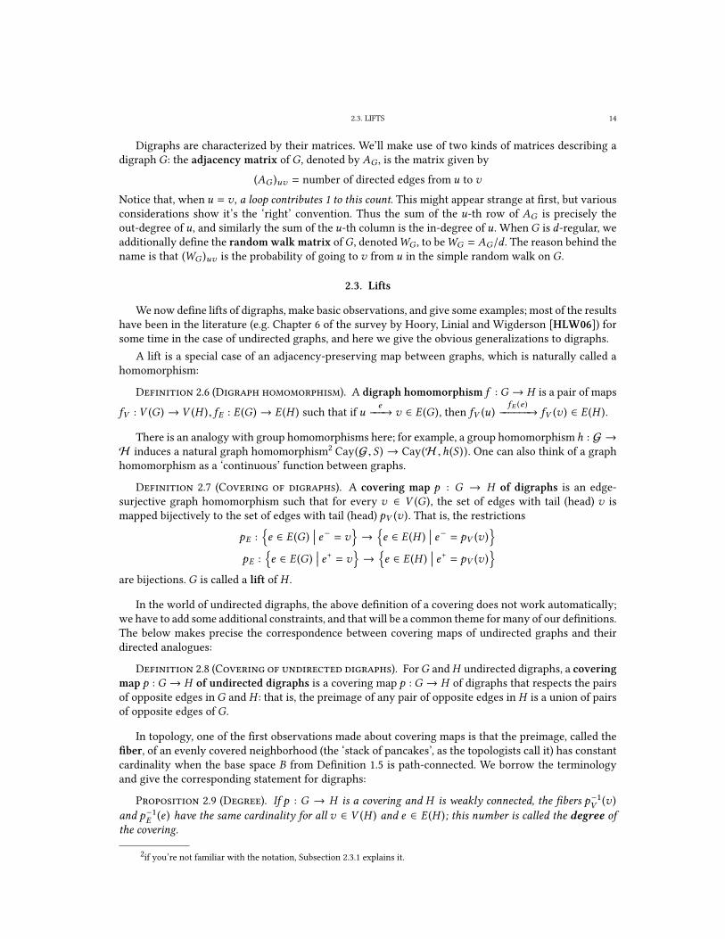
Digraphs are characterized by their matrices. We’ll make use of two kinds of matrices describing a
digraph G: the adjacency matrix of G, denoted by AG , is the matrix given by
(AG )uv = number of directed edges from u to v
Notice that, when u = v , a loop contributes 1 to this count. This might appear strange at �rst, but various
considerations show it’s the ‘right’ convention. Thus the sum of the u-th row of AG is precisely the
out-degree of u, and similarly the sum of the u-th column is the in-degree of u. When G is d-regular, we
additionally de�ne the random walk matrix ofG, denotedWG , to beWG = AG/d . The reason behind the
name is that (WG )uv is the probability of going to v from u in the simple random walk on G.
2.3. Lifts
We now de�ne lifts of digraphs, make basic observations, and give some examples; most of the results
have been in the literature (e.g. Chapter 6 of the survey by Hoory, Linial and Wigderson [HLW06]) for
some time in the case of undirected graphs, and here we give the obvious generalizations to digraphs.
A lift is a special case of an adjacency-preserving map between graphs, which is naturally called a
homomorphism:
Definition 2.6 (Digraph homomorphism). A digraph homomorphism f : G → H is a pair of maps
fV : V (G ) → V (H ), fE : E (G ) → E (H ) such that if ue−−−→ v ∈ E (G ), then fV (u)
fE (e )−−−−−−→ fV (v ) ∈ E (H ).
There is an analogy with group homomorphisms here; for example, a group homomorphism h : G →
H induces a natural graph homomorphism2Cay(G , S ) → Cay(H ,h(S )). One can also think of a graph
homomorphism as a ‘continuous’ function between graphs.
Definition 2.7 (Covering of digraphs). A covering map p : G → H of digraphs is an edge-
surjective graph homomorphism such that for every v ∈ V (G ), the set of edges with tail (head) v is
mapped bijectively to the set of edges with tail (head) pV (v ). That is, the restrictions
pE :
{e ∈ E (G )
∣∣∣ e− = v} → {e ∈ E (H )
∣∣∣ e− = pV (v )}pE :
{e ∈ E (G )
∣∣∣ e+ = v} → {e ∈ E (H )
∣∣∣ e+ = pV (v )}are bijections. G is called a lift of H .
In the world of undirected digraphs, the above de�nition of a covering does not work automatically;
we have to add some additional constraints, and that will be a common theme for many of our de�nitions.
The below makes precise the correspondence between covering maps of undirected graphs and their
directed analogues:
Definition 2.8 (Covering of undirected digraphs). ForG and H undirected digraphs, a covering
map p : G → H of undirected digraphs is a covering map p : G → H of digraphs that respects the pairs
of opposite edges in G and H : that is, the preimage of any pair of opposite edges in H is a union of pairs
of opposite edges of G.
In topology, one of the �rst observations made about covering maps is that the preimage, called the
�ber, of an evenly covered neighborhood (the ‘stack of pancakes’, as the topologists call it) has constant
cardinality when the base space B from De�nition 1.5 is path-connected. We borrow the terminology
and give the corresponding statement for digraphs:
Proposition 2.9 (Degree). If p : G → H is a covering and H is weakly connected, the �bers p−1V (v )
and p−1E (e ) have the same cardinality for all v ∈ V (H ) and e ∈ E (H ); this number is called the degree ofthe covering.
2if you’re not familiar with the notation, Subsection 2.3.1 explains it.

2.3. LIFTS 15
Proof. Suppose we have an edge e = (u ,v ) ∈ E (H ) with u , v . Let Fu = p−1(u), Fv = p−1(v ) and
Fe = p−1(e ) be the �bers. For every x ∈ Fu , since p maps the out-edges of x bijectively to the out-edges
of u, there is exactly one out-edge with image e . Moreover, the tail of every edge in Fe is in Fu because pis a homomorphism. This gives a function f : Fu → Fe which is injective and surjective, so a bijection.
We similarly get a bijection between Fe and Fv , showing that all three sets have the same cardinality.
Reapplying this argument shows that whenever two vertices/edges are connected by a path (ignoring
directions), their �bers have the same cardinality. By connectedness, we conclude the statement of the
proposition. �
Our current view of coverings is not very constructive; it seems hard to give an explicit combinatorial
description of all coverings of a given graph, or to think about them in concrete terms. But the above
proof points to something more useful:
Proposition 2.10 (Covers by permutations on edges). Suppose H is a digraph and S is a set. Then
all lifts3G ofH with degree |S | can be obtained by lettingV (G ) = V (H )×S , and picking bijections fe : S → S
for every e ∈ E (H ), so that the edges of G are precisely es = ((e− , s ), (e+ , fe (s ))) as s ranges over S and eranges over E (H ).
Proof. As we established in the proof of 2.9, ifG → H is a covering, then for any edge e = (u ,v ) ∈E (H ), the �ber Fe gives a perfect matching from Fu to Fv . So a covering certainly �ts the above descrip-
tion. Conversely, given a graph G as in the proposition, we can de�ne a natural map p : G → H by
(v , s ) 7→ v and es = ((e− , s ), (e+ , fe (s ))) 7→ (e− , e+) which is readily seen to be a covering. �
In this thesis we call s a lift coordinate. Given a covering p : G → H of degree d , we will call G a
d-lift, also called a d-cover, of H . Similarly, given a covering p : G → H of the form from the above
proposition, so that V (G ) is identi�ed with V (H ) × S , we will call G an S-lift, also called an S-cover, of
H .
Example 2.11 (Bipartite double cover). For any digraph H , we can de�ne a special {1, 2}-liftG of
H called the bipartite double cover, by assigning to every edge ue−−−→ v of H the transposition (1 2).
It’s then easy to see that G is a bipartite digraph, with the two parts beingV (H ) × {1} andV (H ) × {2}.
As an example, the bipartite double cover of a bouquet of n loops is the graph on two vertices u and v ,
with n directed edges u −−→ v , and n directed edges v −−→ u.
Proposition 2.10 is a fairly trivial observation, but shifting the perspective to edges allows us to con-
struct and think of coverings in very reductionist terms, which will help us a great deal.
Remark 2.12. We remark that if we want to restrict ourselves to undirected digraphs, we have to
make sure that we lift every pair of opposite edges e , e ′ with inverse permutations fe = f −1e ′ .
Finally, the following is immediate by composing the bijections from the de�nition of a covering:
If p : G → H and q : H → K are covering maps, then the composition q ◦ p : G → K is also a
covering map. This allows us to talk about towers of lifts, where we have a sequence of covering maps
Gnpn→ Gn−1
pn−1→ . . . → G1
p1→ G0, and Gi is a lift of G j whenever i > j; this will be our setting for
constructing expander families from lifts.
2.3.1. Cayley and Schreier graphs. An important example of covering maps comes from Cayley
and Schreier graphs, so we’ll devote some time to them. We keep the names ‘Cayley graph’ and ‘Schreier
graph’ used in the literature, but in this thesis all Cayley and Schreier graphs are implicitly digraphs.
Here is the digraph structure:
3This description is redundant, in the sense that there will be many isomorphic lifts obtained through this process. It’s not
hard to see that we can assign the identity permutation to the edges in any tree, and still get all lifts using the remaining freedom;
see [GT87]

2.4. SPECTRAL EXPANSION 16
Definition 2.13 (Cayley and Schreier graphs). For a group G and a multiset S of elements of G,
the Cayley graph Cay(G , S ) is the digraph with vertex set the underlying set of G, and edges д −−→ sдfor every д ∈ G and every s ∈ S . If we’re additionally given a subgroup H ⊂ G, we can also form the
Schreier coset graph Sch(G ,H , S ) with vertex set the left cosets G/H , and edges дH −−→ sдH for
every coset дH and every s ∈ S . Finally, given a set X with a left G-action, we can de�ne the Schreier
graph Sch(G ,X , S ) to be the graph with vertex set X and an edges x −−→ sx for every x ∈ E and s ∈ S .
Clearly, a Cayley graph is a Schreier coset graph where H = id, and a Schreier coset graph is a
Schreier graph for the action of G on left cosets; so a Schreier graph is the most general notion of the
three.
Since in the theory of expanders we often work with undirected graphs, it is desirable to get natural
undirected versions of Cayley/Schreier graphs. This is done by making S a symmetric generating set, so
that S = T ∪T −1 as multisets, where inversion is elementwise. Then we have the natural pairs of opposite
edges u −−→ tu and tu −−→ t −1tu = u, which make Sch(G ,X , S ) into an undirected digraph.
Finally, observe that any Schreier graph Sch(G ,X , S ) covers the bouquet of circles BS , which is the
digraph with one vertex and directed loops in bijection with S : just map every edge coming from the
element s ∈ S to the s-th loop. Since every x ∈ X has exactly one out-edge x −−→ sx labeled by sand exactly one in-edge s−1x −−→ x labeled by s , this gives a covering map. This example will be very
important for us later on.
2.4. Spectral expansion
There are many qualitatively equivalent measures of expansion – De�nition 1.4 is one of them, called
vertex expansion – and we can transition from one to another, losing some quantity along the way;
we refer the reader to Hoory et al [HLW06] and Vadhan [Vad12] for a more comprehensive account.
There is no ‘best’ measure of expansion – the transition functions deteriorate near certain values of the
parameters, and di�erent measures are needed for di�erent applications. In this thesis, we will use the
spectral expansion, which is amenable to algebraic methods:
Definition 2.14 (Spectral expansion). For a digraph G, we de�ne the spectral expansion of G by
λ(G ) = max
x⊥uG
‖WGx ‖
‖x ‖
whereuG is the uniform probability distribution overV (G ), and the maximum4
is over all nonzero vectors
x ∈ RV (G )orthogonal to uG .
The distribution WGπ represents taking a random step backwards in G; a forward step would be
represented by W TG π . The reason for the unusual convention is that we prefer all our actions to be on
the left in this thesis. But this doesn’t matter, since λ(G ) is the second singular value of WG , which is
invariant under matrix transposition – see Proposition 2.18!
We want λ(G ) to be small. Intuitively, λ(G ) is the factor by which the distance from uniformity of
a probability distribution on V (G ) shrinks after taking a single step in the random walk on G; so it’s
not surprising that it tells us a lot about the random walk on G. Alternatively, we can think of x ⊥ uGas a function on the vertices of G that has expectation zero, and of our graph as of trying to estimate
that expectation via ‘sampling’ by the adjacency operatorWG ; how good the estimate is, as measured by
λ(G ), tells us something about how sampling via the random walk looks like random sampling.
In the undirected case, the eigenvalues tell us a lot about the connectivity properties of the graph,
and we can give a more familiar de�nition of λ(G ):
4Note that the use of max instead of sup is justi�ed. By normalization it su�ces to restrict our attention to ‖x ‖ = 1. Orthog-
onal complements are closed in �nite dimensional vector spaces, thus intersecting u⊥ with the sphere gives a closed compact set,
where the continuous function ‖WGx ‖ achieves its supremum.

2.4. SPECTRAL EXPANSION 17
Proposition 2.15 (Undirected spectral graph theory basics). For an undirected d-regular di-graph G = (V , E),
(1) WG has real eigenvalues λ1 ≥ λ2 ≥ . . . ≥ λn with |λi | ≤ 1 and λ1 = 1;(2) 1 is an eigenvalue of multiplicity > 1 i� G is disconnected;
(3) λ(G ) = max {|λ2(G ) |, |λn (G ) |}.Proof. (1) For undirected G, the adjacency matrix and thus the random walk matrix are
symmetric, so we can apply the spectral theorem to get an orthonormal basis of eigenvectors
e1, e2, . . . , en with respective eigenvalues λ1 ≥ λ2 ≥ . . . ≥ λn . Since G is d-regular, we have
WGuG = AGuG/d = duG/d = uG , so the uniform distribution is an eigenvector of eigenvalue
1. Next, we observe thatWG is a contraction in l1 norm, and in particular if f is an eigenvector
with eigenvalue λ, we have
|λ | × ‖f ‖1 = ‖WGf ‖14,≤
∑v∈V
∑u∈V
(WG )vu |fu | =∑u∈V
|fv |∑v∈V
(WG )uv =∑u∈V
|fv | = ‖f ‖1
Since eigenvectors are nontrivial, we conclude that |λ | ≤ 1.
(2) If G is disconnected, pick two connected components Ci and vectors vi constant on Ci and
zero otherwise; then vi are independent eigenvectors of WG with eigenvalue 1. Conversely,
if we have two independent eigenvectors of eigenvalue 1, it’s easy to see by considering the
maximum coordinate that each is constant on connected components; by independence, these
components have to be di�erent!
(3) Observe that for x ⊥ uG , if we decompose x =∑
i αiei along the basis, the e1 = uG component
is 〈x ,uG〉 = 0, so
‖WGx ‖ =n∑i=2
λ2i α2
i ≤ max{|λ2 |, |λn |}2n∑i=2
α 2
i = max{|λ2 |, |λn |}2‖x ‖�
For directed digraphs, we can do something very similar, using the singular value decomposition, a
generalization of the spectral theorem; so here’s a linear-algebraic detour devoted to that:
Definition 2.16. For a matrix A, the singular values of A are the square roots of the eigenvalues of
the symmetric matrix ATA.
It’s easy to see the eigenvalues ofATA are non-negative, so the above de�nition makes sense: suppose
ATAv = λv ; then ‖Av ‖ = vTATAv = vT (λv ) = λ‖vTv ‖ = λ‖v ‖ and hence λ ≥ 0. The singular values
provide something of an analogue of the eigenvalues when the matrix in question is not symmetric:
Theorem 2.17 (Singular value decomposition for real sqare matrices). Any square real n × nmatrix A admits a factorization of the form A = U ΣV T
where:
(1) U andV are n × n orthogonal matrices, and Σ is an n × n diagonal matrix with the singular values
σ1 ≥ . . . ≥ σn on the diagonal.
(2) The columns v1, . . . ,vn of V and the columns u1, . . . ,un of U , called left- and right-singularvectors of A, satisfy
Avi = σiui and ATui = σivi
(3) We are free to choose the columns of V to be any orthonormal basis of eigenvectors for ATA.
Proposition 2.18 (Spectral expansion = second singular value). For a regular digraph G, thesingular values ofWG are 1 = σ1 ≥ σ2 ≥ . . . ≥ 0, and λ(G ) = σ2.

2.5. BASIC EXPANSION PROPERTIES OF LIFTS 18
Proof. This is a generalization of Proposition 2.15, where we made use of the eigenvalue decompo-
sition for symmetric matrices, so here we naturally use the singular value decomposition. First observe
that, since G is both in- and out-regular,W TGWGuG =W
TGuG = uG , and the proof from Proposition 2.15
thatWG is a contraction in l1 norm carries over toW TG to give
‖W TGWGx ‖1 ≤ ‖WGx ‖1 ≤ ‖x ‖1
for any x , hence W TGWG is also a contraction in l1. Thus, the eigenvalues of W T
GWG lie in [0, 1]. Next,
pick any x ⊥ uG , and pick a spectral decompositionWG = U ΣV Twhere the �rst column of V is uG , as
provided by 2.17. Decompose x =∑n
i=1αivi in the basis of right-singular vectors; then α1 = 〈x ,uG〉 = 0,
so using the orthonormality of the u1, . . . ,un we compute
‖WGx ‖ =
∥∥∥∥∥∥∥n∑i=2
αiσiui
∥∥∥∥∥∥∥ =√√ n∑
i=2
α 2
i σ2
i ≤ σ2
√√ n∑i=2
α 2
i = σ2‖x ‖
with equality when x is a multiple of v2. �
In analogy with De�nition 1.4, we de�ne the objects we want to construct, hopefully fully explicitly.
Definition 2.19 (Expander families and expander towers). An in�nite family of d-regular di-
graphs G1,G2, . . . with |V (Gn ) | → ∞ is called an expander family if there is a constant λ < 1 such that
λ(Gn ) ≤ λ for all n. It is called an expander tower if, additionally, there are covering maps Gn+1 → Gnfor all n ∈ N.
2.5. Basic expansion properties of lifts
We will think of vectors as functions, so that for example for a set S the vector space CS is identi�ed
with the vector space of functions S → C; this makes the notation more natural. We will identify the
adjacency matrix AG of a graph G with the linear operator on CV (G )given by multiplication on the left:
v 7→ AGv .
The following proposition is the basis of the niceness of coverings with respect to expansion:
Proposition 2.20. If p : G → H is a covering of �nite graphs, and F is any �eld, there is a natural
induced linear transformation Lp : FV (H ) → FV (G )given by f 7→ f ◦ pV which �ts in the following
commutative diagram of vector spaces:
FV (G ) AG // FV (G )
FV (H ) AH //
Lp
OO
FV (H )
Lp
OO
Proof. Denote the standard bases for FV (H )and FV (G )
by (fv )v∈V (H ) and (fv ,s )(v ,s )∈V (G ) . By lin-
earity, it su�ces to prove that for all fv we have AGLpfv = LpAH fv . So �x v and observe that
LpAH fv = Lp
∑e:u→v
fu
=∑s
∑e:u→v
fu ,s
and
AGLpfv = AG
∑s
fv ,s
=∑s
AGfv ,s =∑s
∑e:(u ,s ′)→(v ,s )
fu ,s ′

2.6. LOWER BOUNDS ON SPECTRAL EXPANSION VIA LIFTS 19
In the �rst sum, the coe�cient of fu ,s for arbitrary u and s is precisely the number5
of edges from u to vin H ; in the second sum, the coe�cient of fu ,s is the size of
S ={e ∈ E (G )
∣∣∣ e− = (u , s ) and e+ = (v , s ′) for some s ′}
Since pE maps the edges with tail (u , s ) bijectively to the edges with tailu, and any edge with head (v , s ′)for some s ′ is mapped to an edge with headv , it follows that pE also maps S bijectively to the set of edges
with tail u and head v . Thus, the coe�cients of fu ,s in the two sums are the same. �
We will only need this for R or C. The undirected analogues of the following consequences have long
been known in the literature on lifts (e.g. Bilu and Linial [BL06]):
Corollary 2.21 (Covers can’t expand better). If p : G → H is a covering of digraphs, then:
1. If f : V (H ) → C is an eigenvector of H with eigenvalue λ, then f ◦ pV : V (G ) → C is an eigenvector
of G with eigenvalue λ. Similarly, if f ,д : V (H ) → C are a pair of left- and right-singular vectors with
singular value σ , so are f ◦ pV ,д ◦ pV .2. λ(G ) ≥ λ(H ).
Proof. From Proposition 2.20, it follows that
AG (f ◦ p) = AG (Lpf ) = LpAH f = Lp (λf ) = λ(Lpf ) = λ(f ◦ p)
as we wanted; the analogous argument works for singular vectors. The second part now follows from
the interpretation of λ(G ) as the second singular value/eigenvalue.
�
Thus, whenever we have a covering p : G → H ,G inherits all eigenvalues of H – the old eigenvalues
– and also has new eigenvalues that we want to bound; similarly for singular values.
2.6. Lower bounds on spectral expansion via lifts
How good can spectral expansion be? It’s easy to observe that for any d-regular simple undirected
digraph G with two vertices u ,v a distance > 2 apart, we have λ(G ) ≥ 1/√d . Indeed, pick the vector
xuv = (0, . . . , 1, . . . , −1, . . . , 0) with a 1 in the u-th position and −1 in the v-th position; then λ(G ) ≥
‖WGx ‖/‖x ‖ =√2/d/√2 = 1/
√d . It turns out that this can be improved to 2
√d − 1/d − on (1) for an n-
vertex graph andd �xed. In this section, we will show how to use covering maps to give lower bounds for
λ(G ) of undirected digraphs; later on, we will (somewhat) reduce the directed case to the undirected one.
The following observations are the basis of lower bounds based on lifts; the idea of using the numbers
pvl (G ) is taken from Vadhan [Vad12]:
Notation 2.22. Given a digraph G, denote by pvl (G ) the probability that a random walk started at vcomes back to v after l steps.
Proposition 2.23. For an undirected d-regular digraph H = (V , E) on n vertices,
(1)
∑v∈V pvl (H ) ≤ 1 + (n − 1)λ(H )l
(2) If p : G → H is a covering of digraphs, pvl (H ) ≥ pxl (G ) for any x ∈ p−1(v ).
Proof. (1) It’s a standard calculation that pvl (H ) is the v-th diagonal entry of W lH , hence∑
v∈V pvl (H ) = trW lH . Since H is undirected, the eigenvalues of W l
H are the l-th powers of
the eigenvalues ofWH ; the largest of those is 1, and all others are bounded by λ(H )l , so the �rst
part follows.
5In the proof we implicitly assume charF = 0; the proof in the other case is analogous, though tedious to write.

2.6. LOWER BOUNDS ON SPECTRAL EXPANSION VIA LIFTS 20
(2) Consider a closed walk of length l in G starting at x ∈ p−1(v ); when we project it to H , we get
a closed walk of length l starting atv . Since for every edge ue−−−→ w in H and x ∈ p−1(u) there
is a unique edge xe ′−−−→ y with y ∈ p−1(w ) that is a lift of e , a step-by-step argument shows
that if two walks in G are sent to the same walk in H , they have to be the same in G as well!
Thus, there are fewer l-step closed walks at x in G than at v in H , which implies the result.
�
The point is that sometimes G is simpler to describe than H , so it’s easier to count closed walks in
G than in H . An analogous approach was used by Friedman in [FT05] to bound the second-largest (not
in absolute value) eigenvalue of expanders related to error-correcting codes. As an application, we now
show how the famous Alon-Boppana theorem follows from that approach:
Theorem 2.24 (Alon-Boppana). Given a family ofd-regular connected undirected digraphsG1,G2, . . .with |V (Gn ) | → ∞, we have
λ(Gn ) ≥ 2√d − 1/d − on (1)
Proof. Observe that the in�nite d-regular tree Td , realized as an undirected digraph, covers any
d-regular undirected connected digraph G. The proof is by a simple generalization of the argument for
undirected simple graphs, found in Section 6 of [HLW06]. Fix v0 ∈ V (G ), and de�ne the following
graph: the vertex set consists of all �nite walksw0
e0−−−−→ w1
e1−−−−→ . . .
ek−−−−→ ek+1 withw0 = v0 inG that
don’t backtrack: that is, en+1, en are never a pair of opposite edges inG for all n. There is a directed edge
between two such walks i� one is an extension of the other by one edge. It’s easy to see this de�nes a
d-regular undirected digraph such that the corresponding undirected graph is the in�nite d-regular tree.
The covering map sends a walk ending atw tow , and an edge e between two walks to the edge inG that
gave rise to e (or the opposite edge, if directions don’t match).
By symmetry, pxl (Td ) is independent of x ; so we have to lower bound the closed walks of length lon Td , which is a combinatorial problem. For l odd, that’s zero, but by a counting argument (see Hoory,
Linial and Wigderson [HLW06]) it turns out thatpx2l (Td ) ≥
(2ll
)(d−1) l
(l+1)d 2l ≥(2√d−1)2l
d 2l l 3/2 and hence λ(Gn )2l ≥
|V (Gn ) ||V (Gn ) |−1
(2√d−1)2l
d 2l l 3/2 −1
|V (Gn ) |−1. After taking 2l-th roots, we get our result. �
It turns out that explicit undirected families of expanders (Gn )n∈N that achieve this bound exist, in
the sense that λ(Gn ) ≤ 2√d − 1/d for all n; this was shown in the celebrated paper [LPS88] of Lubotzky,
Phillips and Sarnak, but only for very special degrees d = p + 1 for p prime. Such optimal spectral ex-
panders are called Ramanujan graphs, and recently an existence proof for bipartite Ramanujan graphs
of all degrees was given by Marcus, Spielman and Srivastava [MSS13], using a completely di�erent ap-
proach. We’ll discuss it and give some generalizations in Section 5.2.

CHAPTER 3
Voltage assignments
3.1. Terminology and basic properties
A tool, called a voltage assignment, for describing certain restricted lifts of graphs, was studied by
Gross and Tucker in their book [GT87], which we follow in this section. They used voltage assignments
to tackle the central problem of topological graph theory: given a graph and a topological surface, can
one draw the graph on the surface without edge intersections, and if so, how? In the process of answering
those questions, they found passing to covering surfaces to be useful, which led them to covering graphs
as well.
In short, a voltage assignment is simply an association of an element of some �xed permutation
group G to every edge of a digraph H . Then, as we saw in Proposition 2.10, we can de�ne a covering
map p : G → H where G is obtained using the permutations as matchings between �bers. It’s not
immediately obvious why restricting G to be a proper subgroup of the full permutation group would be
bene�cial at all – we expect that the more freedom to introduce ‘chaos’ we have, the easier it is to make
graphs that look random. Here are some reasons in favor of more abstraction:
• The case when G = Z/kZ has been studied in previous work, where it was shown that expand-
ing lifts do exist in this restricted case, and the representation-theoretic structure of Z/kZ was
used in the analysis [AKM13].
• The study of voltage assignments in the abstract sheds more light on the parallels between lifts
and Cayley/Schreier graphs. Indeed, we will obtain known characterizations of the spectra of
Cayley/Schreier graphs [HLW06] as special cases of the results in Section 3.2.
• Even when the permutations are not restricted to a proper subgroup, when we perform a se-
quence of several lifts, the permutations describing the top lift will be restricted; we will com-
pute exactly how. The short answer turns to be ‘iterated wreath products’, which will help us
understand the construction in [RSW06] better.
It seems that voltage assignments are absent from the recent developments in expansion in lifts;
consequently, we shall see that authors re-invented special cases of some results from the 90s, e.g. Bilu
and Linial and Agarwal, Kolla and Madan [BL06, AKM13]. We shall show how these generalize. We now
review the terminology of Gross and Tucker and some of their basic results, generalizing them in the
obvious manner to digraphs along the way.
Definition 3.1 (Ordinary voltage assignment). Given a digraph G and a group G, an ordinary
voltage assignment is a function α : E (G ) → G. The derived graph associated with α , denoted by Gα,
is the G-lift of G where the permutation on an edge e is the permutation on G given by the left action
α (e ) : д 7→ α (e )д.
Example 3.2. We obtain all Cayley graphs as a special case of derived graphs for ordinary voltage
assignments: if G = BS , and the image of α with multiplicity is S ⊂ G, Gαis exactly Cay(G , S ), as we
discussed in Subsection 2.3.1.
Definition 3.3 (Permutation voltage assignment). Given a digraphG and a group G, a permuta-
tion voltage assignment is a function α : E (G ) → Sym(S ) for some set S . The derived graph associated
with α , denoted by Gα, is the S-lift of G where the permutation on an edge e is α (e ).
21

3.1. TERMINOLOGY AND BASIC PROPERTIES 22
Clearly, since we can realize the left action of a groupG on itself as a subgroup of Sym(G), the derived
graph of an ordinary voltage assignment is a special case of the derived graph of a permutation voltage
assignment. Moreover, as we saw in Proposition 2.10, permutation voltage assignments are expressive
enough to describe all possible lifts. Ordinary voltage assignments, on the other hand, are not: they
correspond to a stronger notion of covering, called regular covering, where the bottom graph is a quotient
of the top graph under a free group action. Gross and Tucker considered one more kind of voltage
assignments:
Definition 3.4 (Relative voltage assignment). Given a graphG, a group G and a subgroupH ⊂
G, a relative voltage assignment is a function α : E (G ) → G. The derived graph associated with α ,
denoted Gα/H, is the lift of G where the permutation on an edge e is the permutation on G/H given by
the left action on cosets α (e ) : дH → α (e )дH .
Example 3.5. We obtain all Schreier coset graphs as a special case of relative derived graphs: ifG = BSand the image of α with multiplicity is S ⊂ G, we have thatGα/H
is exactly Sch(G , G/H , S ), as we saw
in Subsection 2.3.1.
So we arrive at the intuition that ordinary voltage assignments are to relative voltage assignments as
Cayley graphs are to Schreier graphs; we will come back to this several times later on. To specialize the
above notions to undirected digraphs, we simply require that, for a pair of opposite edges, the voltage
assignmentα assigns inverse group elements, in analogy with Remark 2.12. Relative voltage assignments,
while being more abstract, still capture all possible lifts:
Proposition 3.6 (From permutation voltages to relative voltages). If p : G → H is an S-covering of digraphs given by permutation voltages α : E (H ) → Sym(S ), G is isomorphic to the derived
graph H α/Hof the voltage assignment α relative toH = stabSym(S ) (s ) where s ∈ S is arbitrary.
Proof. It su�ces to show that the action of Sym(S ) on the left cosets of H is isomorphic to the
action of Sym(S ) on S by permutations. What do the cosets ofH look like? For t ∈ S , denote the trans-
position between s and t by (s t ) ∈ Sym(S ); then we claim that the cosets are precisely
{(s t )H
∣∣∣ t ∈ S}.
Indeed, any ϕ ∈ Sym(S ) such that ϕ (s ) = t can be written as ϕ = (s t ) (s t )ϕ = (s t ) ((s t )ϕ) and
(s t )ϕ (s ) = (s t ) (t ) = s , hence (s t )ϕ ∈ H , so the coset (s t )H consists of exactly those permutations that
send s to t .
Now it’s clear what to do: de�ne a bijection f : Sym(S )/H → S by (s t )H 7→ t . Suppose we have
ϕ ∈ Sym(S ) such that ϕ (t ) = u; then ϕ sends the coset (s t )H to the coset ϕ (s t )H which is the same as
the coset (s u)H , as ϕ (s t ) (s ) = ϕ (t ) = u. So f gives an isomorphism between the two actions. �
3.1.1. Basic expansion properties. Let’s think about the random walk on the derived graph Gα
for an ordinary voltage assignment α : E (G ) → Sym(n). A vertex in Gαis a pair (v , π ) where v is a
vertex of G and π is a permutation. In a random walk, the v coordinate performs a random walk on
G, and the π coordinate changes as π0, π1π0, . . . , πk . . . π1π0 where π1, . . . , πk are the permutations
assigned to the edges of the random walk in G. Convergence to uniformity means that both the random
walk on G converges to uniform, and the permutation πk . . . π1 converges to uniform. We can interpret
α : E (G ) → Sym(n) as a permutation voltage assignment as well: in this case, the second coordinate will
be a point instead of a permutation, and to approach uniformity we will need πk . . . π1(s ) to approach a
uniformly random point.
Clearly, πk . . . π1 approaching a uniform permutation is a stronger condition than πk . . . π1(s ) ap-
proaching a uniform point; thus, we expect the derived graph from the permutation voltages to be at
least as goon an expander as the one derived from the ordinary voltages. This intuition is matched and
generalized by the following observation:
Proposition 3.7 (Ordinary voltages expand less than relative ones). For a relative voltage
assignment α : E (G ) → G relative toH ⊂ G, there is a natural covering map p : Gα → Gα/H

3.2. SIGNING MATRICES FOR ALL LIFTS 23
Proof. We do the obvious thing: given a vertex (v ,д) ∈ Gα, we map it down to (v ,дH ); given an
edge (v ,д) → (u ,hд) where (v ,u) is lifted by the permutation h, we map it down to (v ,д) → (u ,hдH );this is easily seen to give a covering. �
As a corollary, we see that a Cayley graph covers any of its corresponding Schreier coset graphs – so
constructing Cayley expanders is harder than constructing Schreier expanders.
3.2. Signing matrices for all lifts
Intuitively, given a liftp : G → H , there is a way to block-diagonalize the adjacency matrix of a lift and
to separate the ‘old’ part of the matrix that comes from H from the interesting part. The motivation is to
have a nice algebraic object, which has been called the signing matrix, that captures the new eigenvalues
ofG; it is the block-diagonalized version of AG without the piece coming from H . The reason this works
is that any permutation action of the group G from which we draw the voltages can be ‘diagonalized’ in
a precise sense using the language of representation theory; by linearity, this diagonalization induces a
‘diagonalization’ of the adjacency matrix of G.
In the literature on expanders, this has been observed for simple graphs in very special cases of G by
Bilu and Linial and Agarwal, Kolla and Madan [BL06, AKM13]; in the literature on voltage assignments,
this has been observed for ordinary voltage assignments of simple graphs by Mizuno and Sato [MS95].
Here we use their manipulation to give the obvious generalization to relative voltage assignments and
digraphs, thus capturing all lifts.
3.2.1. Representation theory review. We will make use of some basic results from the represen-
tation theory of �nite groups. Representation theory aims to describe abstract groups by studying the
homomorphisms from such groups to the more concrete setting of linear operators on vector spaces1. A
representation of G is like a ‘manifestation’ of G as a group of linear operators, to which linear algebra
can be applied with the hope of understanding the structure of G better. Representation theory has been
an incredibly successful tool in many areas of mathematics, and, like expanders, is at the intersection of
several �elds; it occasionally makes its way into computer science as well!
We will work with unitary representations, where the setting is that of unitary operators over complex
vector spaces; for �nite groups, this is without loss of generality. Here we barely scratch the surface –
for a comprehensive introduction, we refer the reader to Artin [Art] (who we follow), and Serre [Ser77].
Definition 3.8 (Representation). For a �nite group G, a matrix representation of G is a homo-
morphism ρ : G → GL(V ) for some �nite dimensional complex vector spaceV . The dimension of ρ is
dimV .
Example 3.9. There are two extreme, trivial examples that show up frequently. The trivial represen-
tation hasV = C and ρ (д) = 1 for all д; this representation ‘forgets’ everything about G.
The (left) regular representation has V = CG and ρ (д) = Pд is the permutation matrix associated
to the left action of д on G by h 7→ дh; this representation ‘remembers’ everything about G, and such
representations are called faithful.
Between these two, it’s easy to spot some more representations: given a subgroupH ⊂ G, the (left)
permutation representation of G relative toH hasV = CG/H and ρ (д) = Pд is the permutation matrix
associated to the left action of д on G/H by hH 7→ дhH ; by takingH to be G or the trivial group, we
get the above examples.
1Any group G can be seen as a category with one element CG , and a homomorphism from G to a vector space is a functor
from CG to the category of vector spaces. Thus, representation theory is somewhat similar to algebraic topology, which considers
functors, like homology and homotopy, from the category of topological spaces to the category of groups. The main point is that
in both cases the target category is better understood in some sense. For more on categories, see Section 4.7

3.2. SIGNING MATRICES FOR ALL LIFTS 24
Example 3.10. Let’s consider a cyclic group Z/k/Z. We know that roots of unity behave like elements
of Z/kZ, and they feel like a ‘manifestation’ of Z/kZ. Can we get some representations out of that?
Indeed, we can: let ω be a primitive k-th root of unity, and for any t ∈ {0, . . . , k − 1}, de�ne the map
ft : Z/kZ→ C given by a 7→ ω ta. Then every ft gives us a 1-dimensional representation of Z/kZ.
In the world of �nite groups, any representation is conjugate to a restricted kind of representation
called a unitary representation:
Definition 3.11. For a �nite group G, a unitary representation of G is a homomorphism ρ : G →
U(V ) for some �nite dimensional Hermitian inner product spaceV .
Permutation representations are clearly unitary. The main fact we need about unitary representations
is that any such representation decomposes orthogonally into a direct sum of irreducible ones:
Definition 3.12 (Irreducible representation). For a representation ρ : G → GL(V ), a subspace
W ⊂ V is invariant under ρ if ρ (д)W ⊂ W for all д ∈ G. A representation is irreducible if it has no
proper invariant subspace.
Theorem 3.13 (Maschke). For any unitary representation ρ : G → U(V ), there is a unique, up to
isomorphism, orthogonal decompositionV =⊕
iVi where eachVi is invariant under ρ, and the restrictionρ : G → U(Vi ) is an irreducible unitary representation.
Example 3.14. For any permutation representation ρ : G → U(CG/H ), there is a one-dimensional
invariant subspace spanned by the all ones vector; this gives a copy of the trivial representation sitting
inside ρ.
For the symmetric group Sym(n), the standard representation is what’s left after we take out the
copy of the trivial representation from the permutation representation of Sym(n) on {1, . . . ,n}. The
standard representation is irreducible, but a proof of that is beyond the scope of this thesis.
Example 3.15. The representations of Z/kZ we found are unitary, as ω taω ta = 1, and are irreducible
by virtue of being 1-dimensional. In fact, it turns out that (see Artin [Art]) they are all irreducible repre-
sentations of Z/kZ, and the regular representation Z/kZ decomposes as a their direct sum!
3.2.2. Tensor product of matrices. We will also make use of the tensor product of matrices, which
has a number of nice properties we state without proof.
Definition 3.16. For matrices A and B, the tensor product A ⊗ B is de�ned by the block matrixa11B . . . a1mB...
. . ....
an1B . . . anmB
The following is a straightforward exercise in matrix manipulation:
Fact 3.17. The matrix tensor product has the following properties (whenever the corresponding matrix
dimensions match):
(1) Bilinearity: (A + B) ⊗ C = A ⊗ C + B ⊗ C , A ⊗ (B +C ) = A ⊗ B +A ⊗ C .(2) Associativity: (A ⊗ B) ⊗ C = A ⊗ (B ⊗ C ).(3) Mixed product: (A ⊗ B) (C ⊗ D) = (AC ) ⊗ (BD), in particular (A ⊗ B)−1 = A−1 ⊗ B−1.
3.2.3. The computation. In this section we use the trick of Mizuno and Sato [MS95] to compute
signing matrices for all lifts. In this section, for matrices Ai , let
⊕i Ai denote the block-diagonal matrix
with blocks Ai . Here is the main observation:
Theorem 3.18 (General signing matrices). Let α : E (G ) → G be a voltage assignment on an N -
vertex digraph G relative to H ⊂ G, and ρG/H the left permutation representation of G relative to H .
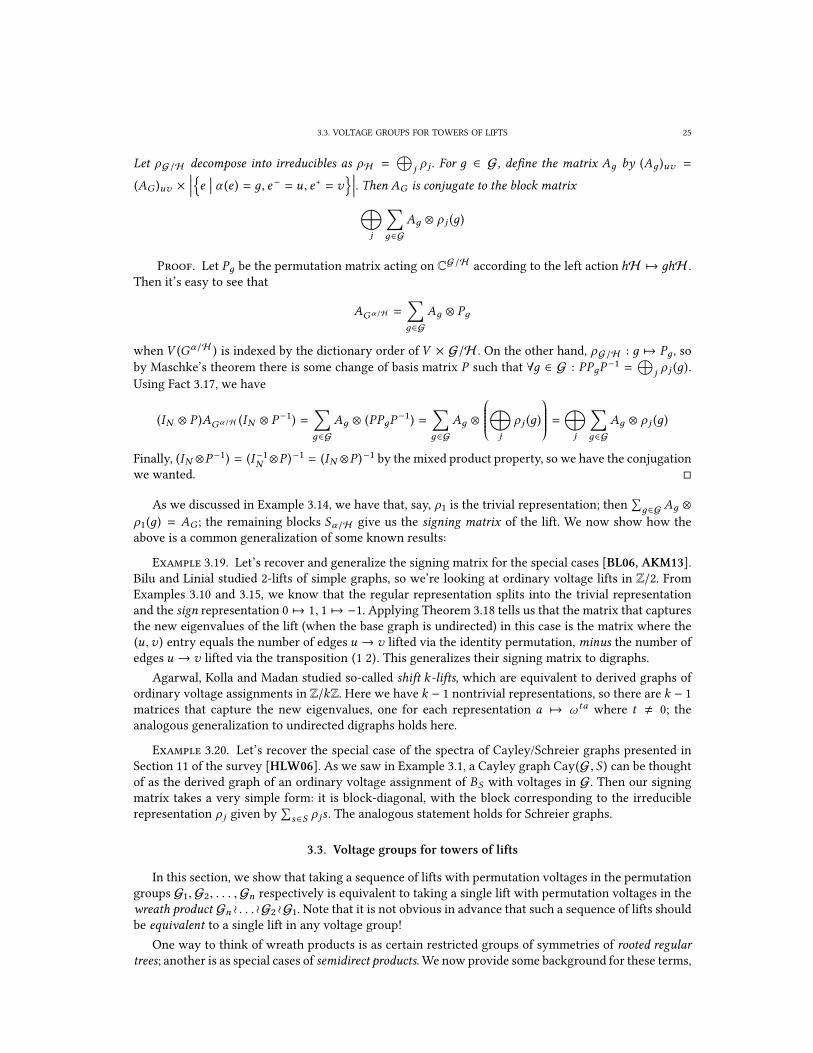
3.3. VOLTAGE GROUPS FOR TOWERS OF LIFTS 25
Let ρG/H decompose into irreducibles as ρH =⊕
j ρ j . For д ∈ G, de�ne the matrix Aд by (Aд )uv =
(AG )uv ×∣∣∣∣{e ∣∣∣ α (e ) = д, e− = u , e+ = v}∣∣∣∣. Then AG is conjugate to the block matrix⊕
j
∑д∈G
Aд ⊗ ρ j (д)
Proof. Let Pд be the permutation matrix acting on CG/H according to the left action hH 7→ дhH .
Then it’s easy to see that
AGα/H =∑д∈G
Aд ⊗ Pд
when V (Gα/H ) is indexed by the dictionary order of V × G/H . On the other hand, ρG/H : д 7→ Pд , so
by Maschke’s theorem there is some change of basis matrix P such that ∀д ∈ G : PPдP−1 =
⊕j ρ j (д).
Using Fact 3.17, we have
(IN ⊗ P )AGα/H (IN ⊗ P −1) =∑д∈G
Aд ⊗ (PPдP−1) =
∑д∈G
Aд ⊗
⊕j
ρ j (д)
=⊕j
∑д∈G
Aд ⊗ ρ j (д)
Finally, (IN ⊗P−1) = (I −1N ⊗P )
−1 = (IN ⊗P )−1
by the mixed product property, so we have the conjugation
we wanted. �
As we discussed in Example 3.14, we have that, say, ρ1 is the trivial representation; then
∑д∈G Aд ⊗
ρ1(д) = AG ; the remaining blocks Sα/H give us the signing matrix of the lift. We now show how the
above is a common generalization of some known results:
Example 3.19. Let’s recover and generalize the signing matrix for the special cases [BL06, AKM13].
Bilu and Linial studied 2-lifts of simple graphs, so we’re looking at ordinary voltage lifts in Z/2. From
Examples 3.10 and 3.15, we know that the regular representation splits into the trivial representation
and the sign representation 0 7→ 1, 1 7→ −1. Applying Theorem 3.18 tells us that the matrix that captures
the new eigenvalues of the lift (when the base graph is undirected) in this case is the matrix where the
(u ,v ) entry equals the number of edges u → v lifted via the identity permutation, minus the number of
edges u → v lifted via the transposition (1 2). This generalizes their signing matrix to digraphs.
Agarwal, Kolla and Madan studied so-called shift k-lifts, which are equivalent to derived graphs of
ordinary voltage assignments in Z/kZ. Here we have k − 1 nontrivial representations, so there are k − 1matrices that capture the new eigenvalues, one for each representation a 7→ ω ta
where t , 0; the
analogous generalization to undirected digraphs holds here.
Example 3.20. Let’s recover the special case of the spectra of Cayley/Schreier graphs presented in
Section 11 of the survey [HLW06]. As we saw in Example 3.1, a Cayley graph Cay(G , S ) can be thought
of as the derived graph of an ordinary voltage assignment of BS with voltages in G. Then our signing
matrix takes a very simple form: it is block-diagonal, with the block corresponding to the irreducible
representation ρ j given by
∑s∈S ρ js . The analogous statement holds for Schreier graphs.
3.3. Voltage groups for towers of lifts
In this section, we show that taking a sequence of lifts with permutation voltages in the permutation
groups G1, G2, . . . , Gn respectively is equivalent to taking a single lift with permutation voltages in the
wreath product Gn o . . . o G2 o G1. Note that it is not obvious in advance that such a sequence of lifts should
be equivalent to a single lift in any voltage group!
One way to think of wreath products is as certain restricted groups of symmetries of rooted regular
trees; another is as special cases of semidirect products. We now provide some background for these terms,

3.3. VOLTAGE GROUPS FOR TOWERS OF LIFTS 26
loosely following [RSW06]; the semidirect product will be useful again in our discussion of the zig-zag
product later on.
3.3.1. Semidirect products and wreath products. We know from group theory a natural way to
‘put two groups G and H together’: just take the direct product G × H , which treats the two groups
independently. When there is some interaction between the two groups, one can de�ne a generalization
of the direct product called the semidirect product. One motivation comes from solving the following
extension problem: suppose we have a short exact sequence of groups
1 // Gα // K
β // H // 1,
that is, α is an injective homomorphism, β is a surjective homomorphism, and imα = ker β . Suppose we
know G and H ; can we recover K ? Intuitively, the short exact sequence is telling us that K should be
in some sense ‘assembled’ from G and H . In the case of abelian groups, which comes up frequently in
homological algebra, if we require the existence of a homomorphism γ : H → K such that β ◦γ = idH ,
the sequence is said to split, andK = G ⊕H . For general groups however, failure of γ (H ) being normal
in K complicates things, and instead K is a semidirect product G o H 2. More concretely, one way to
de�ne the semidirect product which is convenient for us is
Definition 3.21. Suppose we have groups G andH , and that φ : H → Aut(G) is a homomorphism
to the right automorphism group of G, i.e. H acts on G on the right by automorphisms φh . Then the
semidirect product G oφ H with respect to φ is the group with underlying set G × H and group law3
(д1,h1) ◦ (д2,h2) = (φh2(д1)д2,h1h2)
It’s immediate that this indeed de�nes a group structure with identity element (idG , idH ). The wreath
product is a special case of the semidirect product for permutation groups:
Definition 3.22. Suppose G andH are �nite permutation groups acting on sets SG , SH respectively.
Then the wreath product G o H is the semidirect product GSH oH with the action of h ∈ H on GSH
is given by permuting the coordinates as φh : (д1,д2, . . .) 7→ (дh(1) ,дh(2) , . . .).
Note that it is somewhat confusing that this gives a right action on GSH , but you can easily verify for
yourself that it does! It turns out that the wreath product naturally inherits the structure of a permutation
group:
Proposition 3.23. The group G o H acts faithfully on the set SG × SH in a natural manner.
Proof. Given µ ∈ GSH and π ∈ H , we de�ne the action of (µ , π ) ∈ GoH on a point (s , t ) ∈ SG ×SHas (µ , π ) (s , t ) = (µt (s ), π (t )). We have to verify this is indeed an action of G o H . The identity element
has µ = (idG , . . . , idG ) and π = idH so it �xes every (s , t ). Next, for (µ ′, π ′) ∈ G o H , we have
(µ ′, π ′)[(µ , π ) (s , t )] = (µ ′, π ′) (µt (s ), π (t )) = (µ ′π (t )µt (s ), π′π (t ))
and
[(µ ′, π ′) ◦ (µ , π )](s , t ) = [φπ (µ′)µ , π ′π ](s , t ) = (µ ′π (t )µt (s ), π
′π (t ))
Finally, assuming (µ , π ) (s , t ) = (µ ′, π ′) (s , t ) for all (s , t ) gives us µt (s ) = µ ′t (s ) and π (t ) = π ′(t ) for all
s , t , from which µ = µ ′ and π = π ′ so the action is faithful. �
2A way to remember which factor goes on which side of the o is to keep in mind the short exact sequence: the order is the
same.
3The reason for the somewhat non-standard convention of using φh2
(д1)д2 instead of д1φh1 (д2) has to do with issues of
handedness in the discussion that follows: one of the actions that arise is more natural as a right action, and we’d rather keep in
mind one right action than keep dragging around inverses.

3.3. VOLTAGE GROUPS FOR TOWERS OF LIFTS 27
3.3.2. Automorphisms of regular rooted trees and iterated wreath products. Our central example
of wreath products comes from the automorphism groups of regular trees; in fact, they provide such a
convenient visualization of wreath products and make so many of their properties obvious that they are
arguably the ‘right’ way to think about wreath products.
Notation 3.24. Let TS1 , . . . ,Sn stand for the rooted tree of depth n in which every node at distance i < nfrom the root has children labelled by the elements of the set Si+1.
To describe a vertex in this tree, we can give the tuple of labels along the unique path from the root:
so the root is represented by the empty tuple () and in general (s1, s2, . . . , sn ) stands for the sn-th child
of the sn−1-th child of . . . of the s1-th child of the root. Any automorphism ofTS1 , . . . ,Sn must carry the set
of leaves bijectively to itself, and thus the set of nodes a distance one from a leaf bijectively to itself, and
so on, inductively we see that every level is carried to itself bijectively; moreover, nodes with a common
parent are carried to children of the image of that parent.
Thus, to describe an automorphism of TS1 , . . . ,Sn it su�ces to give, for each vertex (s1, . . . , si ) at dis-
tance i < n from the root, an element πs1 , . . . ,s i ∈ Sym(Si+1) according to which the children of that
vertex are permuted. Then the automorphism ϕ described by these permutations moves vertices by
ϕ : (s1, s2, . . . , si ) 7→ (π() (s1), πs1 (s2), . . . , πs1 , . . . ,s i−1 (si ))
This formula captures the similarity to the wreath product, and much more. Now consider the restricted
automorphism group of TS1 , . . . ,Sn with respect to the groups Gi ⊂ Sym(Si ), where a node at distance ifrom the root can permute its children only by elements of some permutation group Gi+1.
Proposition 3.25. The wreath product is associative, and in fact the restricted automorphism group of
TS1 , . . . ,Sn with respect to Gi ⊂ Sym(Si ) is Gn o . . . o G1, realized as a permutation group on the set of leaves
S1 × . . . × Sn .
Proof. The proof is by induction on n: the main point is that the automorphism group is completely
determined by the permutations it induces on the leaves! For n = 1 there is nothing to prove. For n = 2,
the automorphism that acts by π on the root and by µs on s ∈ S1 acts on S1 × S2 in the same way as
G2 o G1, and since the action is faithful, the automorphism group is isomorphic to G2 o G1.
For n > 2, assume for now right-associative notation for wreath products. DenoteTn = TS1 , . . . ,Sn and
Tn−1 := TS1 , . . . ,Sn−1 . We can imagine replacing the subtreeTn−1 by the depth-1 treeTS1× . . .×Sn−1 with the
same set of leaves. Since the restricted automorphism group ofTn−1 is Gn−1 o . . . o G1 by hypothesis, and
where the leaves can go depends only on where their parents can go and the group Gn , we see that the
leaves of Tn can be permuted in the same way by the restricted automorphism group of Tn and that of
TS1× . . .×Sn−1 ,Sn with respect to Gn−1 o . . . o G1 and Gn , By the case n = 2, the latter permutation group is
Gn o Gn−1 o . . . o G1, and it equals the group we wanted to �nd.
Finally, here’s a sketch proof of associativity: if we have a depth-3 tree T , there are two ways we
can split it into depth-1 and depth-2 trees; replacing the depth-2 trees by depth-1 trees as in the above
induction step gives us the restricted permutation groups (G3 o G2) o G1 and G3 o (G2 o G1) on the leaves of
T ; but these should both equal the restricted automorphism group of T with respect to G1, G2, G3! �
We also describe some common inclusions into the iterated wreath product that will be helpful in
Section 5.1:
Example 3.26. Given Gn o . . . o G1, there is a natural inclusion Gm o . . . o G1 ↪→ Gn o . . . o G1 whenever
m < n by mapping an automorphism of the �rst m levels to an automorpism on the �rst n levels that
acts by the identity permutation on every node below them-th level. There is the ‘orthogonal’ inclusion
(Gn o . . . o Gm+1)S1× . . .×Sm ↪→ Gn o . . . o G1 by acting on the �rst m levels trivially, and permuting the
children of the leaf (s1, . . . , sm ) ofTS1 , . . . ,Sm via the (s1, . . . , sm )-th coordinate. The special casesm = n−1andm = 1 will be useful in Section 5.1.

3.3. VOLTAGE GROUPS FOR TOWERS OF LIFTS 28
Example 3.27. For any Gn o . . . o G1, there is an inclusion G1 × . . . × Gn ↪→ Gn o . . . o G1 obtained by
sending (д1, . . . ,дn ) to the automorphism that acts by дi on every node at level i .
3.3.3. The computation. Here is the main observation4:
Proposition 3.28 (Voltage groups of towers). Suppose we have a sequence of covering mapsGnpn→
Gn−1pn−1→ . . . → G1
p1→ H , where pi is obtained by permutation voltages in the permutation group Gi acting
on the set Si . Then the composition p1◦ . . .◦pn : Gn → H is obtained by permutation voltages in Gn o . . . oG1.
Conversely, given any covering p : G → H with permutation voltages in Gn o . . . o G1, it corresponds toa tower of lifts of the above kind.
Proof. This is really all about the case n = 2; the rest is induction. So, we induct on n: for n = 1,
there is nothing to prove, and we will establish the n = 2 case later; now suppose that for some k ∈ N,
the assertion holds true with n = k . Let G̃k = Gk o . . . o G1 and S̃k = Sk × . . . × S1. For the �rst direction,
let p̃k = p1 ◦ . . . ◦ pk . Then we have coverings Gk+1pk+1→ Gk
p̃k→ H , and by the induction hypothesis p̃k
is obtained by permutation voltages in G̃k which acts on S̃k . Using the case n = 2, this means that the
composition p̃k ◦ pk+1 is obtained by permutation voltages in Gk+1 o G̃k = Gk+1 o . . . o G1 as we wanted.
For the other direction, we have a lift with voltages in Gk+1 o . . . o G1 = Gk+1 o G̃k . Using the case n = 2,
this means that we have a sequence of coverings Gk+1pk+1→ Gk
p̃k→ H where pk+1 has voltages in Gk+1,
and p̃k has voltages in G̃k . Applying the induction hypothesis to p̃k , we’re done.
It remains to establish the case n = 2; it su�ces to think about a single edge ue→ v in H , and what
permutations it can be assigned by our lifts. For the forward direction, let e be assigned π ∈ G1 byp1, thus
lifting to S1 edges; then let the one with tail (v , s ) be assigned µs ∈ G2 by p2. The resulting permutation
σ on S1 × S2 that is assigned to e by p1 ◦ p2 is then given by
σ (s1, s2) = (π (s1), µs1 (s2))
Now consider the depth-2 rooted tree T where the root has children labelled by S1, and each child has
leaves labelled by S2: then the leaves are in bijection with S1 × S2, and as we saw in Proposition 3.23, the
above formula means that σ is precisely an element of its restricted automorphism group G2 o G1.
For the reverse direction, given a covering p : G → H with permutation voltages in G2 o G1 and a
permutation σ ∈ G2 o G1 assigned to e , represent sigma as an element ((. . . , µs , . . .), π ) ∈ GS12o G1 of
the automorphism group ofT . Then reasoning analogously to the previous direction, we see that lifting
e according to π and then lifting the copy of e with tail (v , s ) according to µs gives us exactly G; the
intermediate lift K �ts into the diagram Gp2
→ Kp1→ H that we wanted to �nd.
�
4This is easy once one knows the answer; the proof we present here was optimized for conciseness. The way one comes up
with the result in the �rst place is by considering the case n = 2, realizing G1 and (G2)S1 as certain natural subgroups of the
conjectured voltage group of p1 ◦ p2, and then reasoning about their interaction to arrive at a semidirect product.
CHAPTER 4
Lifting graph operations
It turns out that several common graph operations that have useful e�ects on expansion respect cov-
ering maps, in the sense that, for an operation α , ifG → H is a covering, we get a covering α (G ) → α (H ).This is perhaps not so surprising for well-behaved operations with an ‘algebraic’ �avor, like powering
and tensoring, but it also works for the more ‘twisted’ derandomized graph products, namely the zig-zag
product of Reingold, Vadhan and Wigderson [RVW02] that is the cornerstone of elementary explicit
constructions of expanders, the generalized zig-zag product of Ben-Aroya and Ta-Shma [BATS11], and
the derandomized square of Rozenman and Vadhan [RV05] that is related to the zig-zag product and was
used to give an alternative proof that L = SL. It seems the reason all these results work is because these
graph operations are de�ned locally, and local structure is preserved by lifts. We remark that the result
on zig-zag products was independently observed by Cooper, Dotterrer and Prassidis [CDP06]. We also
introduce a graph product, called the backward-forward square, which can be used instead of the ordinary
square in iterative constructions where we desire undirected graphs, and which allows us to translate
expanding towers of directed graphs into expanding towers of undirected graphs without terrible losses
– so we don’t have to worry too much about issues of directedness!
We will use these operations’ compatibility with covering maps as the key step in a general technique
to iteratively construct expanding towers of coverings inspired by a construction by Rozenman, Shalev
and Wigderson [RSW06] in Section 5.1. Another implication of these results is that whenever we have
an expanding tower, we can apply any of our operations to all graphs in it to translate it to another
expanding tower. Since various classical explicit constructions of expanders can be tweaked to give an
expanding tower of Cayley/Schreier graphs, this gives us a way of producing some new expander families
from them.
The operations we introduce act in various ways on number of vertices, degree and expansion, so it’s
convenient to de�ne
Definition 4.1. An (n,d , λ)-graph is a d-regular digraph G on n vertices with λ(G ) ≤ λ; similarly,
an (N ,D , λ)-graph is a D-regular digraph G on vertex set N with λ(G ) ≤ λ.
4.1. Rotation maps and their lifts
A rotation map is a way of keeping track of edges in graphs by specifying labels to the edges incident
to each vertex and the way these labels interact. Rotation maps were initiated by Reingold, Vadhan
and Wigderson in [RVW02], where they were used to de�ne and study the zig-zag product. They were
further generalized by Rozenman and Vadhan in [RV05] to directed graphs; this is the source we follow
in this section (except when talking about lifts).
Rotation maps are useful when we want to reason about multigraphs where there might be many
edges between a pair of vertices, and when we want to reason about the explicitness of various operations
on graphs (which can be encoded in terms of their rotation maps). In this section, we state the de�nition
of a rotation map for directed and undirected digraphs, and prove some basic facts about the interaction
between rotation maps and coverings.
Definition 4.2. For a d-regular digraph G = (V , E), we de�ne a two-way labelling to be, for each
v ∈ V , a pair of bijections
{e ∈ E
∣∣∣ e− = v} → D and
{e ∈ E
∣∣∣ e+ = v} → D for some set D with |D | = d .
29

4.1. ROTATION MAPS AND THEIR LIFTS 30
In other words, giving a two-way labeling to a digraph is making it into a D-regular graph.
Notation 4.3. For a digraphG and a two-way labeling lG ofG, we will write (G; lG ) for the version of
G labeled by lG . We will use the (G; lG ) notation whenever there might be confusion about which labels a
digraph is given; if there is an obvious labeling from context, we just write G. Whenever we have an edge
ue−−−→ v with label i at u and j at v , we will denote it by u
i e j−−−−→ v to simplify notation. When the name
of the edge is not important, we omit it.
Definition 4.4. For a D-regular digraphG, de�ne the rotation map ofG with respect to the labeling
to be the function RotG : V (G ) × D → V (G ) × D given by
RotG (u , i ) = (v , j ) when ui j−−−→ v ∈ E (G )
Observe that the rotation map completely speci�es the graph and the two-way labelling, and it is a
permutation of V (G ) × D. We will very often encode a rotation RotG (u , i ) = (v , j ) by the more visually
appealing ui j−−−→ v ∈ E (G ). The corresponding notion for undirected graphs needs some additional
structure:
Definition 4.5. For an undirected digraphG, an (undirected) two-way labeling is a two-way label-
ing of G where we require that if ui e j−−−−→ v ∈ E (G ), the edge opposite to e is labeled as v
j e ′ i−−−−−→ u.
Another property of two-way labelings we will need later on is
Definition 4.6. A digraph G is called consistently two-way labeled if, for every edge, the label at
the tail is the same as the label at the head.
Given the ‘local’ view of a graph that rotation maps give us, it’s expected that given a covering of
graphs and a rotation map for the base graph, there is a natural way to de�ne a rotation map for the lift.
It is fortunate that the formula for the rotation map is the same in the directed and undirected cases: the
conventions from De�nition 4.5 and Remark 2.12 take care of this behind the scenes.
Proposition 4.7. Suppose p : G → H = (V , E) is a covering of directed (respectively undirected) d-regular digraphs via permutation voltage assignment π : E → Sym(S ), and H is a directed (respectively
undirected) two-way labeled digraph with rotation map RotH . Then there is a natural induced rotation map
on G given by
RotG ([v , s], i ) = ([u , πe (s )], j )
where (u , j ) = RotH (v , i ) and e is the i-th edge out of v . Moreover, if H is consistently labeled, G inherits
such a labeling.
Proof. This is a routine computation. First, let’s deal with directed digraphs. Observe that G in-
herits a two-way labeling by composing the labeling on H with the bijections
{e ∈ E (G )
∣∣∣ e± = v} pE→{
e ∈ E (H )∣∣∣ e± = pV (v )}. This induces a rotation map on G. Consider a vertex [v , s] ∈ V (G ), and let
vi e j−−−−→ u in H . Then, if es is the lift of e with tail [v , s], by the de�nition of the labelling in G we have
[v , s]i es j−−−−−→ [u , πes] which encodes the rotation map we wanted.
For undirected digraphs, we need to verify that G inherits an undirected two-way labeling from H .
So consider a pair of opposite edges vi e j−−−−→ u and u
j e ′ i−−−−−→ v in H . Let es be the lift of e with tail
[v , s] and e ′s the lift of e ′ with tail [u , πes]; since by convention we assign inverse permutations to pairs
of opposite edges, the head of e ′s is [v , π −1e πes] = [v , s]. So by the previous paragraph, in G we have the
pair of opposite edges [v , s]i es j−−−−−→ [u , πes] and [u , πes]
j e ′s i−−−−−→ [v , s], as needed. Finally, it’s obvious
from our de�nition of the two-way labeling on G that if H is consistently labeled, so is G. �

4.2. POWERING 31
The above result is in a particularly simple form: it says that to obtain the rotation map of the lift, we
simply need to ‘insert’ one more coordinate, a lift coordinate, in the rotation map of the base, and change
that coordinate according to the relevant permutation; moreover, it applies equally well to directed and
undirected graphs. It will be convenient to de�ne the following terms:
Definition 4.8. A labeled covering map p : (G; lG ) → (H ; lH ) of S-regular digraphs is a covering
map of digraphs p : G → H such that, when H is given labels lH , the labels induced on G by the process
from Proposition 4.7 are lG ; clearly the composition of labeled covering map is again a labeled covering
map.
Notation 4.9. For a cover p : G → H and an edge ui j−−−→ v ∈ E (H ), denote the permutation assigned
by p to that edge by πu ,i .
4.1.1. Graphs that cover BS . Later on, we will be very interested in which digraphs cover a bouquet
of circles. We provide two points of view: one via two-way labelings, the other via Schreier graphs:
Proposition 4.10. For an |S |-regular digraph G, the following are equivalent:
(1) There exists a covering map p : G → BS ;(2) There is a consistent two-way labeling of G;(3) G is a Schreier graph.
Proof. (1) ⇐⇒ (2): For the forward direction, if an edge ofG projects to the s-th loop of BS , label
that edge by s on the head and tail. Since p is a covering map, the out-labels at each vertex are in bijection
with S , and so are the in-labels at each vertex. For the backward direction, given such a labeling, project
an edge us s−−−−→ v to the s-th loop; since the labeling is valid, it gives a covering map.
(2) ⇐⇒ (3): The method used here is similar to the one Gross used [Gro77] to show that any
connected undirected regular digraph of even degree is a Schreier coset graph. For the forward direction,
observe that, for every s ∈ S , the map πs : V (G ) → V (G ) given by v 7→ u where vs s−−−−→ u ∈ E (G ) is a
permutation, since every u has a unique in-edge and out-edge labeled by s at u. Letting G ⊂ Sym(V (G ))
be the group of permutations generated by T ={πs
∣∣∣ s ∈ S}, we see that G is exactly Sch(G ,V (G ),T ).
For the reverse direction, notice that in an |S |-regular Schreier digraph, every edge us−−−→ v has a
natural name given by the generator s that gives rise to it. Then labeling it as us s s−−−−→ v gives us a
consistent two-way labeling. �
Example 4.11. SupposeG is an undirected digraph of even degree 2d . Then Gross [Gro77] (notice that
the paper works in the generality of undirected multigraphs) tells us1
that every connected component of
G can be realized as the Schreier coset graph of some groupG with respect to some symmetric generating
set S = T ∪T −1. Thus we have a covering map from every component of G to B2d , which when joined
together give us a covering map G → B2d . Notice that, however, it’s not obvious how to compute a
Schreier structure on G e�ciently!
4.2. Powering
4.2.1. De�nition and expansion properties. Powering is a basic graph operation that takes a graph
and forms another graph on the same vertex set where the edges correspond to length k walks in the
original graph. Formally,
Definition 4.12. For a digraph G, the k-th powerGkof G is the graph with vertices V (Gk ) = V (G )
and edges given by all k-step walks on G:
E (Gk ) ={(e1, . . . , ek )
∣∣∣ ei ∈ E (G ) and e+i = e−i+1}
1Also see the discussion after Theorem 11.16 in Hoory et al [HLW06].

4.2. POWERING 32
with (e1, . . . , ek )− = e−
1and (e1, . . . , ek )
+ = e+k . When G is two-way labeled, the standard choice of
rotation map is
RotGk (w0, (l1, l2, . . . , lk )) = (wk , (rk , rk−1, . . . , r1))
where the right side is de�ned inductively by wi−1l i r i−−−−−→ wi ∈ E (G ).
Moreover, this preserves undirected graphs: if G comes with an undirected two-way labeling, the
above rotation map is easily seen to induce an undirected two-way labeling on Gk.
The random walk onGkis a random walk onG that takes k steps at a time, so we can think of it as a
‘k times faster’ copy of the random walk onG. Correspondingly, we expect it to converge to the uniform
distribution k times faster! Since in our bounds time is in the exponent of λ2, we expect the spectral
expansion of Gkto be λ(G )k . Indeed, a standard calculation gives AGk = (AG )
k, and thus
Proposition 4.13. For an (n,d , λ)-digraph G, Gkis an (n,dk , λk )-digraph.
Proof. When walking a d-regular digraph, there are d choices at each step for the next edge to take;
thus the number of k-step walks out of any given vertex is dk . Similarly, there are d edges to come from,
so the k-step walks that end at any given vertex are also dk . Next, sinceWG preserves the subspace uG ,
it preserves the orthogonal complement u⊥G , and thus for any x ⊥ uG we have
‖WGkx ‖ = ‖ (WG )kx ‖ = ‖WG (W
k−1G x )‖ ≤ λ‖ (WG )
k−1x ‖ ≤ . . . ≤ λk ‖x ‖
�
We remark that when G is undirected, using the eigenvalues this can be strengthened to say that in
fact λ(Gk ) = λ(G )k ; but for general digraphs, no such result holds (see footnote 5 in [RV05]).
4.2.2. Lifting properties. The main observation in this section is that graph powering ‘respects’
covering maps:
Proposition 4.14. If p : G → H is a labeled covering map, there is a natural labeled covering map
q : Gk → H kfor all k . Moreover, this is compatible with undirected graphs: if G → H is a covering of
undirected digraphs, so will be q.
Proof. Suppose we have an edge w0
(l1 , . . . ,lk ) (rk , . . . ,r1)−−−−−−−−−−−−−−−−−→ wk ∈ E (H
k ) coming from a walk
w0
l1 e1 r1−−−−−−−→ w1
l2 e2 r2−−−−−−−→ . . . −−→ wk−1
lk ek rk−−−−−−−→ wk
in H . Then every edge in that walk gives rise to edges in the lift G; in particular, we have edges
(w0, s )l1 r1−−−−−→ (w1, πe1s ) ∈ E (G ), (w1, πe1s )
l2 r2−−−−−→ (w2, πe2πe1s ) ∈ E (G ),
. . . , (wk−1, πek−1 . . . πe1s )lk rk−−−−−→ (wk , πekπek−1 . . . πe1s ) ∈ E (G )
These in turn de�ne an edge in E (Gk ):
(w0, s )(l1 , . . . ,lk ) (rk , . . . ,r1)−−−−−−−−−−−−−−−−−→ (wk , πekπek−1 . . . πe1s ) ∈ E (G
k )
Since the permutation πek−1 . . . πe1 is uniquely determined by w0 and l1, . . . , lk , this means that Gk
is exactly the labeled cover of H kwhere the (l1, . . . , lk )-th edge out of w0 lifts via the permutation
πek . . . πe1!
To deal with undirected graphs, observe that if p : G → H is a covering of undirected digraphs, then
the permutations assigned to opposite edges in H kare πek . . . πe1 and π −1e1 . . . π
−1ek , which are inverses of
each other, so pk : Gk → H kis a covering of undirected digraphs as well! �

4.3. TENSORING 33
4.3. Tensoring
4.3.1. De�nition and expansion properties. The tensor product of two graphs, as the name sug-
gests, is the tensor product of their corresponding adjacency matrices:
Definition 4.15. For digraphs G and H , the tensor product G ⊗ H is the digraph with adjacency
matrix AG⊗H = AG ⊗ AH .
The adjacency matrix hides some of the information if we care about the labels; but there is a natural
way to track which edge of G ⊗ H comes from which edges of G and H , and so we can give a de�nition
in terms of rotation maps:
Definition 4.16. For two-way labeled regular digraphs G and H , the tensor product G ⊗ H is the
regular digraph with vertex set V (G ) × V (H ), and rotation map
RotG⊗H ((u ,u′), (l , l ′)) = ((v ,v ′), (r , r ′))
where ul r−−−−→ v ∈ E (G ) and u ′
l ′ r ′−−−−−→ v ′ ∈ E (H ).
It’s easy to check this gives the same digraph. Thus, we can think of the random walk on the tensor
productG ⊗H as two simultaneous, independent copies of the random walks onG and H . Each of these
approach uniformity at some rate, so we would expect the combined walk to approach uniformity at
the rate of the walk that approaches uniformity more slowly; for example, imagine that the H walk
takes longer to approach uniformity, and consider a walk on G ⊗ H that starts out as uniform on each
V (G ) × {v}: then it’s easy to see this walk is a ‘blown-up’ version of the random walk on H .
This is indeed the case, but before we can prove that, we will need the following
Fact 4.17. For square matrices A and B with singular values σ1, . . . , σn and µ1, . . . , µm , the singularvalues of A ⊗ B are {
σiµ j∣∣∣ 1 ≤ i ≤ n, 1 ≤ j ≤ m
}With this, we easily prove our intuition is right:
Corollary 4.18. λ(G1 ⊗G2) = max{λ(G1), λ(G2)}, so in particular, ifG1 is an (n1,d1, λ1) graph, andG2 is an (n2,d2, λ2) graph, then G1 ⊗ G2 is an (n1n2,d1d2,max{λ1, λ2})-graph.
Proof. We know thatWG1,WG2
have singular values 1 ≥ σ2 ≥ . . . ≥ 0 and 1 ≥ µ2 ≥ . . . ≥ 0; hence
the second singular value ofWG1⊗WG2
is the larger of σ2 × 1 and 1 × µ2. �
4.3.2. Lifting properties. It turns out that tensoring is also compatible with lifts. Some intuition for
that comes from the observation that the tensor product G ⊗ H when H is d-regular can be thought of
as a special lift of the graph obtained by replacing each edge of G by d identical copies of itself. This is
not surprising if we recall the proof of Theorem 3.18 where we made heavy use of tensors! Here is the
general statement:
Proposition 4.19. If p1 : G1 → H1 and p2 : G2 → H2 are respectively a labeled S1- and labeled S2-covering of digraphs, there is a natural induced S1 × S2-covering map q : G1 ⊗G2 → H1 ⊗ H2. Moreover, if
pi are coverings of undirected digraphs, so is q.
Proof. Let’s have edges uil i e i r i−−−−−−→ vi ∈ E (Hi ). These give rise to the edge (u1,u2)
(l1 ,l2) (r1 ,r2)−−−−−−−−−−−−→
(v1,v2) ∈ E (H1 ⊗ H2). We can now de�ne an S1 × S2 lift of H1 ⊗ H2 by lifting the latter edge via the
product permutation of S1 × S2 that acts independently on the factors by π (i )(u i ,l i )
; that is, the rotation
map of the lift is encoded by
[(u1,u2), (s1, s2)](l1 ,l2) (r1 ,r2)−−−−−−−−−−−−→
[(v1,v2),
(π (1)u1 ,l1
(s1), π(2)u2 ,l2
(s2))]

4.4. THE BACKWARD-FORWARD SQUARE AND UNDIRECTING 34
On the other hand, ei give rise to edges (ui , si )l i r i−−−−−→
(vi , π
(i )u i ,l i
si)∈ E (Gi ) in the respective lifts.
These combine to give an edge
[(u1, s1), (u2, s2)](l1 ,l2) (r1 ,r2)−−−−−−−−−−−−→
[(v1, π
(1)u1 ,l1
s1),(v2, π
(2)u2 ,l2
s2)]∈ E (G1 ⊗ G2)
We see that this is the same rotation map as that of the S1×S2 lift we de�ned – only the order in which we
give the coordinates of a vertex are di�erent. The covering map is obtained by mapping [(u1, s1), (u2, s2)]down to (u1,u2), and so on.
Finally, compatibility with undirected digraphs is a straightforward exercise; the key is that the in-
verse of the product permutation is the component-wise inverse. �
Remark 4.20. Notice that this covering map is not exactly of the form p : G → H where V (G ) =V (H ) × S : the two lift coordinates s1 and s2 are ‘split’. But it is equivalent to such a covering map up
to a natural isomorphism of the vertex set of G1 ⊗ G2 – namely, the one that permutes the factors of
V (H1) × S1 × V (H2) × S2 to get toV (H1) × V (H2) × S1 × S2. This will happen again in our next proofs.
Proposition 4.19 seems to be a fairly general statement, and it’s worth considering several special
cases. For example, it’s easy to check that we obtain a well-known result about Cayley/Schreier graphs
as a special case when the coverings p1,p2 are of bouquets, as in Examples 3.2, 3.5:
Corollary 4.21. We have Cay(G1, S1) ⊗ Cay(G2, S2) = Cay(G1 × G2, S1 × S2), and more generally
Sch(G1,A1, S1)⊗Sch(G2,A2, S2) = Sch(G1 × G2,A1 ×A2, S1 × S2) where the action of G1 × G2 onA1 ×A2
is the product action (д1,д2) (a1, a2) = (д1a1,д2a2).
Another special case is obtained by using a trivial covering for p2:
Corollary 4.22. If p : G → H is a labeled covering of S-regular digraphs, and K is any digraph, there
is an induced covering map q : G ⊗ K → H ⊗ K .
Then making the graph K from the latter Corollary a bouquet we recover another familiar operation:
Definition 4.23. For a digraphG with a two-way labeling and a numberd , de�ne the edge duplicated
graph dG to be the two-way labeled digraph obtained fromG by duplicating every edge d times, so that
the d copies of an edge ui j−−−→ v are labeled as u
(i ,k ) ( j ,k )−−−−−−−−−→ v for k ranging over {1, . . . ,d}.
The e�ect on the adjacency matrix of G is multiplication by d : AdG = dAG , hence λ(dG ) = λ(G ). It’s
easy to see that edge duplication is compatible with covering:
Corollary 4.24. If p : G → H is a labeled covering of regular digraphs, and Bd is the bouquet of dloops where the head and tail of the i-th loop is labeled by i , we have a labeled covering q : G ⊗ Bd = dG →dH = H ⊗ Bd .
4.4. The backward-forward square and undirecting
Here we de�ne two natural graph operations that allow us to translate results about directed ex-
panders to results about undirected ones in a way compatible with covering maps. Given G, our �rst
operation is given by simply superimposing G with the graph obtained from G by reversing all edges,
following Ben-Aroya and Ta-Shma [BATS11]; this has a natural structure of an undirected digraph. Our
second operation is like the square, but instead of two forward steps we do a backward step followed by a
forward step; the motivation is that the adjacency matrix will beATGAG , which is symmetric and naturally
related to λ(G ) by Proposition 2.18. Thus the e�ect on expansion is like squaring, with the additional ben-
e�t that we get undirected graphs! We will use this backward-forward square to give a directed analogue
of the Alon-Boppana Theorem 2.24, and to get undirected expanding towers from directed ones.

4.4. THE BACKWARD-FORWARD SQUARE AND UNDIRECTING 35
4.4.1. De�nition and expansion properties.
Definition 4.25. For a D-regular digraph G, the undirection of G is the D × {−1, 1}-regular undi-
rected digraph G† with an opposite pair of edges u(i ,1) ( j ,1)−−−−−−−−→ v ,v
( j ,−1) (i ,−1)−−−−−−−−−−−→ u ∈ E (G†) for every
edge ui j−−−→ v ∈ E (G ). The backward-forward square of G, denoted GTG, is the D2
-regular digraph
with vertex set V (G ), and rotation map
RotGTG[v , (i′, j )] = [w , (j ′, i )]
whenever we have the following edges:
ui i ′−−−−→ v ∈ E (G ), u
j j ′−−−−→ w ∈ E (G ).
As promised, we have2
Proposition 4.26. For any D-regular two-way labeled digraph G, G† is an undirected D × {−1, 1}-regular digraph that inherits an undirected two-way labeling, has adjacency matrixAG +AT
G , and λ(G†) ≤
λ(G ). Similarly, GTG is an undirected D2-regular digraph that inherits an undirected two-way labeling,
has adjacency matrix ATGAG , and λ(G
TG ) = λ(G )2.
Proof. For the undirection, everything is obvious except spectral expansion; for this observe that
since G† is 2|D |-regular,WG† = 1/2(WG +W TG ). Then for any x ⊥ uG , we have ‖WG†x ‖ ≤ 1/2(‖WGx ‖ +
‖W TG x ‖) ≤ 1/2(λ(G ) + λ(G )) = λ(G ), as singular values are invariant under transposition. Next, by the
de�nition of the backward-forward square, for an edgev(i ′ , j ) ( j ′ ,i )−−−−−−−−−→ w ∈ E (GTG ), we also have an edge
w( j ′ ,i ) (i ′ , j )−−−−−−−−−→ v , and it’s natural to pair these two to giveGTG the structure of an undirected digraph. As
the labels of the two edges at bothv andw match, and moreover any loop this is an undirected two-way
labeling. Next, we count
(AGTG )vw =∑
u∈V (G )
(AG )uv (AG )uw =∑
u∈V (G )
(ATG )vu (AG )uw = (AT
GAG )vw
By regularity, this means WGTG = W TGWG . As we saw in ??, λ(G ) is the second singular value of WG ,
which is exactly the square root of the second eigenvalue ofW TGWG , and we’re done. �
Corollary 4.27 (Lower bounds on λ(G ) for directed graphs). Given a family of d-regular di-
graphs G1,G2, . . . with |V (Gn ) | → ∞, λ(Gn ) ≥√2√d − 1/d − on (1).
To see this, just apply Theorem 2.24 to GT1G1,G
T2G2, . . ., or G†
1,G†
2, . . .
4.4.2. Lifting properties.
Proposition 4.28. Suppose p : G → H is a labeled S-covering of D-regular digraphs. Then there are
natural labeled covering maps q : GTG → HTH , r : G† → H † of undirected digraphs.
Proof. Let’s have an edge v(i ′ , j ) ( j ′ ,i )−−−−−−−−−→ w ∈ E (HTH ) coming from the two edges
ui i ′−−−−→ v ∈ E (H ), u
j j ′−−−−→ w ∈ E (H )
For any s ∈ S , these two de�ne edges in the lift:
(u , s )i i ′−−−−→ (v , πu ,is ) ∈ E (G ), (u , s )
j j ′−−−−→ (w , πu , js ) ∈ E (G )
2It transpired after submission of this thesis that compatibility with lifts fails for the backward-forwards square because we
weren’t careful enough with loops; it turns out that our correspondence between undirected graphs and digraphs has to allocate
pairs of opposite edges for loops as well! After this change, the proposition still works for undirecting under a slight change in the
de�nition of the rotation map.

4.5. ZIG-ZAG PRODUCT AND GENERALIZED ZIG-ZAG PRODUCT 36
which in turn mean we have the edge (v , πu ,is )(i ′ , j ) ( j ′ ,i )−−−−−−−−−→ (w , πu , js ) ∈ E (G
TG ). Relabeling S according
to π −1u ,i , this gives
∀s ∈ S : (v , s )(i ′ , j ) ( j ′ ,i )−−−−−−−−−→
(w , πu , jπ
−1u ,is
)∈ E (GTG )
and hence GTG is the lift of HTH where the (i ′, j )-th edge out of (v , s ) is assigned the permutation
πu , jπ−1u ,i . The permutation assigned to the reverse edgew
( j ′ ,i ) (i ′ , j )−−−−−−−−−→ v is then πu ,iπ
−1u , j = (πu , jπ
−1u ,i )
−1;
thus, pairs of opposite edges inHTH lift to pairs of opposite edges inGTG, as we wanted. The veri�cation
for the undirection follows an analogous idea. �
4.5. Zig-zag product and generalized zig-zag product
The zig-zag product of Reingold, Vadhan and Wigderson [RVW02] marks a turning point in the work
on explicit constructions of expanders, as it demonstrated how to construct good expander families by
an elementary and intuitive combinatorial argument.
4.5.1. De�nition and expansion properties.
Definition 4.29. For two-way labeled regular digraphsG and H withG aV (H )-regular digraph and
H a D-regular digraph, the zig-zag productG z©H is the D2-regular graph with vertex set V (G ) × V (H )
and rotation map
RotG z©H [(v , k ), (i , j )] = [(w , l ), (j ′, i ′)]
whenever we have the following edges:
ki i ′−−−−→ k ′ ∈ E (H ), v
k ′ l ′−−−−−→ w ∈ E (G ), l ′
j j ′−−−−→ l ∈ E (H )
This seems very complicated! Here’s an intuitive idea: let’s think of the setV (G ) ×V (H ) as a version
ofV (G ) where every vertex was blown up to a cloud in bijection withV (H ). Starting at the k ∈ V (H )-thvertex of the cloud of v ∈ V (G ), a single step under the label (i , j ) in the zig-zag product can be thought
of as:
• a step within the v-cloud following label i , arriving at the k ′-th vertex in the cloud;
• a step between clouds, guided by k ′ interpreted as an edge label inG, to thew cloud. The in-label
l ′ of the v → w edge tells us at which vertex of the w cloud we land;
• a step within the w-cloud following label j.
Example 4.30. It will be convenient to keep some (half-)trivial examples in mind. Consider the zig-zag
productBS z©K of a bouquet of circlesBS on one vertex ∗with any |S |-regular digraphK , and suppose that
BS is consistently labeled. We can ignore the ∗ and think of it as a graph on the set V (H ). To determine
RotBS z©K [k , (i , j )], we look at the edges
ki i ′−−−−→ k ′ ∈ E (K ), ∗
k ′ k ′−−−−−→ ∗ ∈ E (BS ), k
′j j ′−−−−→ l ∈ E (K )
and conclude that the result is [l , (j ′, i ′)], hence BS z©K = K 2.
The amazing thing about the zig-zag product is that it essentially inherits spectral expansion from
both G and H , but degree only from H ! This is the what makes the zig-zag product so successful in the
spectral setting. Amazingly, the proof of the following Theorem uses only basic linear algebra!
Theorem 4.31 (Vadhan [Vad12]; Reingold-Vadhan-Wigderson [RVW02]). If G is an (n,m, λG )-digraph andH is an (m,d , λH )-digraph, then for any two-way labeling ofG andH ,G z©H is an (nm,d2, λG+2λH )-digraph; furthermore, if G and H are undirected, G z©H is an undirected (nm,d2, λG + λH )-digraph.

4.5. ZIG-ZAG PRODUCT AND GENERALIZED ZIG-ZAG PRODUCT 37
This was used by Reingold, Vadhan and Wigderson in [RVW02] to give an elementary, combinatorial
fully-explicit construction of expanders by an iterative process. The considerations behind this construc-
tion will be important for us later on, when we make constructions of expanding towers based on these
ideas.
Example 4.32 (Fully explicit expanders from the zig-zag product). Intuitively, we want to start
with some good expander, and perform a sequence of operations (one of them being the zig-zag product)
that gives us back a bigger graph with bounded expansion and the same degree.
One idea is to start with H being a (d 4 ,d , λ)-digraph, and inductively de�ne
Gn+1 = G2
n z©H , G1 = H 2
Then it’s easy to see that Gn has d 4nvertices, and as long as λ is a small enough constant (which is
achievable by, say, brute-force search), (Gn )n∈N will be an expander family of d2-regular graphs. How-
ever, here we only get mild explicitness; the reason is that to evaluate the rotation map ofGn+1, we need
to make two calls to the rotation map of H , but also two calls to the rotation map of Gn . Since the depth
of the recursion is n, this leads to exponentially many in n = O (log(d 4n )) queries at the bottom!
To remedy this, Reingold, Vadhan and Wigderson used the following trick to make the recursion
shallower: for H a (d8,d , λ)-digraph, let G1 = H 2,G2 = H ⊗ H , and then
Gn+1 =(G d n
2e ⊗ G b n
2c
) 2z©H
Then Gn will be a d2-regular digraph on d8n
vertices with bounded expansion if λ is small. But the time
T (n) to compute a rotation map in Gn is now about T (n) ≈ 4T (n/2) + c , because we need two rotations
fromG d n2e , two rotations fromG b n
2c , and two rotations from H . The recursion solves to a polynomial in
n = O (log(d8n )).
We remark that constructions based on the zig-zag product can achieve λ = O (d3/4/d ) (andO (d2/3/d )with some extra work), which is better than constant, but still not as good as Ramanujan graphs.
4.5.2. Relationship to the semidirect product. Alon, Lubotzky and Wigderson [ALW01] found
that, somewhat surprisingly, the zigzag product of Cayley graphs is a Cayley graph of the semidirect
product with a suitable choice of generators:
Fact 4.33 (Zig-zag product and semidirect product). For groups G and H with H acting on G,
Cay(G , S ) z©Cay(H ,T ) is a Cayley graph Cay(G oH ,U ) of the semidirect product when the generating
sets S and T are chosen suitably; for example, when S is a single T -orbit.
This is suspiciously similar to the wreath products from Chapter 3. It is natural to ask if this can
be used as a basis for a construction of expanding towers, and indeed, we shall see in Subsection 5.1.1
how this idea was used by Rozenman, Shalev and Wigderson to construct expanding towers via the
relationship between coverings and the wreath product!
Another reason this is intriguing is that it feels very similar to Corollary 4.21; so there are reasons to
believe that Fact 4.33 can be a special instance of a much more general phenomenon. Thus, an immediate
question for future work is the following:
�estion 4.34. How do we generalize Fact 4.33 in the same way that Proposition 4.19 generalizes
Corollary 4.21?
4.5.3. Lifting properties. It turns out that there is a simpler relationship between zig-zag products
and coverings that is somewhat surprising: given a labeled covering G → H , we get a labeled covering
G z©K → H z©K . Intuitively, one reason for that is that every edge in H z©K comes from a unique edge in
H (the edge between clouds). Using the permutation on this edge induced by the covering map G → H ,
we can de�ne a lift of H z©K ; this lift turns out to be naturally isomorphic to G z©K !
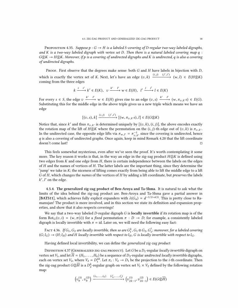
4.5. ZIG-ZAG PRODUCT AND GENERALIZED ZIG-ZAG PRODUCT 38
Proposition 4.35. Suppose p : G → H is a labeled S-covering of D-regular two-way labeled digraphs,
and K is a two-way labeled digraph with vertex set D. Then there is a natural labeled covering map q :
G z©K → H z©K . Moreover, if p is a covering of undirected digraphs and K is undirected, q is also a covering
of undirected digraphs.
Proof. First observe that the degrees make sense: both G and H have labels in bijection with D,
which is exactly the vertex set of K . Next, let’s have an edge (v , k )(i , j ) ( j ′ ,i ′)−−−−−−−−−→ (w , l ) ∈ E (H z©K )
coming from the three edges
ki i ′−−−−→ k ′ ∈ E (K ), v
k ′ l ′−−−−−→ w ∈ E (H ), l ′
j j ′−−−−→ l ∈ E (K )
For every s ∈ S , the edge vk ′ l ′−−−−−→ w ∈ E (H ) gives rise to an edge (v , s )
k ′ l ′−−−−−→ (w , πv ,k ′s ) ∈ E (G ).
Substituting this for the middle edge in the above triple gives us a new triple which means we have an
edge
[(v , s ), k](i , j ) ( j ′ ,i ′)−−−−−−−−−→ [(w , πv ,k ′s ), l] ∈ E (G z©K )
Notice that, since k ′ and thus πv ,k ′ is determined uniquely by [(v , k ), (i , j )], the above encodes exactly
the rotation map of the lift of H z©K where the permutation on the (i , j )-th edge out of (v , k ) is πv ,k ′ .In the undirected case, the opposite edge lifts via πw ,l ′ = π
−1v ,k ′ since the covering is undirected, hence
q is also a covering of undirected graphs. Once again, keep in mind Remark 4.20 that the lift coordinate
doesn’t come last! �
This feels somewhat mysterious, even after we’ve seen the proof. It’s worth contemplating it some
more. The key reason it works is that, in the way an edge in the zig-zag product H z©K is de�ned using
two edges from K and one edge from H , there is certain independence between the labels on the edges
of H and the names of vertices of H . The latter labels are the important thing, since they determine the
‘jump’ we take in K ; the niceness of lifting comes exactly from being able to lift the middle edge to a lift
G of H , which changes the names of the vertices of H by adding a lift coordinate, but preserves the labels
k ′, l ′ on the edge.
4.5.4. The generalized zig-zag product of Ben-Aroya and Ta-Shma. It is natural to ask what the
limits of the idea behind the zig-zag product are. Ben-Aroya and Ta-Shma gave a partial answer in
[BATS11], which achieves fully explicit expanders with λ(Gn ) = d−1/2+o(1) . This is pretty close to Ra-
manujan! The product is more involved, and in this section we state its de�nition and expansion prop-
erties, and show that it also respects coverings!
We say that a two-way labeled D-regular digraph G is locally invertible if its rotation map is of the
form RotG (v , i ) = (w , π (i )) for a �xed permutation π : D → D; for example, a consistently labeled
digraph is locally invertible with π = id. Later on, we will need the following easy fact:
Fact 4.36. IfG1,G2 are locally invertible, then so areGk1,G1 ⊗G2,G
†
1; moreover, for a labeled covering
(G; lG ) → (H ; lH ) and H locally invertible with respect to lH , G is locally invertible with respect to lG .
Having de�ned local invertibility, we can de�ne the generalized zig-zag product:
Definition 4.37 (Generalized zig-zag product). LetG be aD1-regular locally invertible digraph on
vertex setV1, and letH = (H1, . . . ,Hk ) be a sequence of D2-regular undirected locally invertible digraphs,
each on vertex set V2, where V2 = D4k1
. Let πi : V2 → D1 be the projection to the i-th coordinate. Then
the zig-zag product G z©H is a Dk2-regular graph on vertex set V1 × V2 de�ned by the following rotation
map: (v (1)0,v (2)
0
) (i1 , . . . ,ik ) (i ′k , . . . ,i′1)
−−−−−−−−−−−−−−−−−→(v (1)2k−1,v
(2)2k−1
)∈ E (G z©H )

4.6. DERANDOMIZED SQUARING 39
whenever we have the following sequence of edges, for j = 1, 2, . . . , 2k − 1:
v (1)j−1 = v
(1)j and v (2)
j−1
i t i ′t−−−−−→ v (2)
j ∈ E (Ht ) whenever j = 1 (mod 2) where t = (j + 1)/2
v (1)j−1
π1(v (2)j−1
)π1
(v (2)j
)−−−−−−−−−−−−−−−→ v (1)
j ∈ E (G ) whenever j = 0 (mod 2), and
v (2)j is additionally determined by πi (v
(2)j ) = πi (v
(2)j−1) for all 1 < i ≤ 4k
As Ben-Aroya and Ta-Shma show, G z©H will also be locally invertible – but it is possibly a directed
graph, sinceHk might be di�erent fromH1! Guaranteeing expansion is not that straightforward anymore:
it relies on a probabilistic argument for the existence of a good H . Fortunately, it can be shown that a
good H exists for all D1-regular locally invertible graphsG! This was noticed by the anonymous referee
of [BATS11], and will be important for us in Subsection 5.1.53
With this, we have
Theorem 4.38 (Theorem 2 and Theorem 7 from Ben-Aroya and Ta-Shma [BATS11]). Suppose
G is a locally invertible (V1,D1, λ1)-digraph, and H = (H1, . . . ,Hk ) a sequence of undirected (V2 =
D4k1,D2, λ2)-digraphs that is ε-good with respect to every D1-regular graph and satis�es λ2 ≤ 1/2. Then
G z©H is an (V1 × V2,Dk2, λk−1
2+ 2(ε + λ1) + λ
k2)-digraph. Moreover, for large enough D1 and D2, ε-good H
exist with ε = D−k2
and λ2 = 2√|D2 | − 1/|D2 | + ε .
Finally, we arrive at the lifting property for the generalized zig-zag product; the philosophy behind
why it works turns out to be the same as for the ordinary zig-zag product.
Proposition 4.39. Suppose p : K → G is a labeled S-covering of D1-regular locally invertible graphs,G
has vertex set V1, and H = (H1, . . . ,Hk ) is a sequence of D2-regular locally invertible undirected digraphs,
each on vertex set V2 = D4k1. Then there is a natural labeled covering map q : K z©H → G z©H .
Proof. First, clearly the zig-zag products can be taken, and both result in Dk2-regular graphs. Next,
suppose we have an edge
(v (1)0,v (2)
0
) (i1 , . . . ,ik ) (i ′k , . . . ,i′1)
−−−−−−−−−−−−−−−−−→(v (1)2k−1,v
(2)2k−1
)∈ E (G z©H ) arising from edges
in G and H as in the de�nition above. Then the edges in G give rise to edges in the lift:
∀s ∈ S , j ≡ 0 (mod 2) : (v (1)j−1, s )
π1(v (2)j−1
)π1
(v (2)j
)−−−−−−−−−−−−−−−→
(v (1)j , πv (1)
j−1 ,π1(v (2)j−1
)s) ∈ E (K )
and in particular, letting µ j−1 = πv (1)j−1 ,π1
(v (2)j−1
)whenever j is even and choosing the values for s induc-
tively, we have (with the convention µ−1 = id)
∀s ∈ S , j ≡ 0 (mod 2) : (v (1)j−1, µ j−3 . . . µ1s )
π1(v (2)j−1
)π1
(v (2)j
)−−−−−−−−−−−−−−−→
(v (1)j , µ j−1µ j−3 . . . µ1s
)∈ E (K )
Combining these edges with the edges from H , we get the existence of an edge
∀s ∈ S : (v (1)0, s ,v (2)
0)
(i1 , . . . ,ik ) (i ′k , . . . ,i′1)
−−−−−−−−−−−−−−−−−→ (v (1)2k−1, µ2k−1 . . . µ1s ,v
(2)2k−1) ∈ E (K z©H )
As usual, since the permutations µi are completely determined by v (1)0,v (2)
0and (i1, . . . , it ), this encodes
the rotation map of a cover of G z©H such that the covering map respects the labels. �
4.6. Derandomized squaring
4.6.1. De�nition and expansion properties. The derandomized square is a close cousin of the zig-
zag product, and is also a sort of derandomized graph product: for a d-regular digraphG, the derandom-
ized square ofG has degree linear in d , but spectral expansion only slightly worse than the expansion of
G2(hence the name)!
3Thus, I’d like to thank the anonymous referee, whoever they are! :)

4.7. CATEGORIES? 40
Definition 4.40. For two-way labeled digraphs G and H with G a V (H )-regular graph and H a T -
regular graph, the derandomized square G s©H of G with respect to H is the V (H ) × D-regular graph
with vertex set V (G ) and rotation map
RotG s©H [v , (k , i )] = [w , (k ′, i ′)]
when we have the following edges:
vk l−−−−→ u ∈ E (G ), l
i i ′−−−−→ l ′ ∈ E (H ), u
l ′ k ′−−−−−→ w ∈ E (G )
As with the zig-zag product, this is somewhat complicated. The intuition is that we �rst take a step in
G freely, but the next step is restricted by the small graph H . And here is the promised spectral expansion
bound:
Theorem 4.41 (Rozenman and Vadhan, [RV05]). If G is an (n,m, λ)-digraph and H is an (m,d , µ )-digraph, then for any choice of two-way labelings, G s©H is a (n,md , λ2 + µ )-digraph.
4.6.2. Lifting properties. The derandomized square enjoys a lifting property analogous to the one
for the zig-zag product; it is similarly somewhat mysterious, but it works for the same reason the zig-zag
one worked. The proof is very similar, so it’s deferred to the appendix: see Proposition A.2.
Proposition 4.42. Suppose p : G → H is a labeled S-covering of T -regular two-way labeled digraphs,
andK is a two-way labeled digraph on vertex setT . Then there is a natural labeled coveringmapq : G s©K →H s©K .
4.7. Categories?
In this section, which can be skipped in a �rst reading, we remark that a simple way to state most of
the results in this chapter is via category theory. The language of categories allows us to formulate and
think about the results in this chapter in a clearer way, and points us to possible generalizations.
Category theory is a sort of metamathematics that studies common patters in mathematical struc-
tures; for example, algebraic topology – which is where category theory originated – is based on common
patterns in the world of topological spaces and groups. Category theory provides us, via functors and
natural transformations, with a way to translate the world of topological spaces to that of groups in a
highly consistent manner. The bene�t is that the world of algebra seems to be easier to understand than
that of topology, and this approach has been very successful in giving us topological - and sometimes
algebraic - insights. Beyond that, category theory helps us generalize various concepts in mathematics,
and give a common perspective on many of them; we refer the interested reader to the classical book by
Mac Lane [ML71]; here we only scratch the surface.
Definition 4.43. A category C is a collection4
of objects obC and a collection of morphisms homC,
such that every morphism f ∈ homC has a sourceX ∈ obC and target Y ∈ obC, denoted as f : X → Y .
Moreover, every object X has a designated identity morphism idX , and for any two morphisms f : X →Y ,д : Y → Z , there is a composite morphism д ◦ f : X → Z . Furthermore, we require that:
• For any f : X → Y , f idX = f = idY f ;
• For any f : X → Y ,д : Y → Z ,h : Z → T , we have h ◦ (д ◦ f ) = (h ◦ д) ◦ f .
Example 4.44. Topological spaces with morphisms being continuous maps form the category Spaces;
groups with morphisms being group homomorphisms form Groups; sets with morphisms being total
functions form Sets, . . .
4We run into set-theoretic issues if we use ‘set’ instead of collection, because we want to talk about e.g. the category of sets,
which cannot be a set because of Russell’s paradox. But don’t worry, because "...the whole concept of a category is essentially
an auxiliary one; our basic concepts are essentially those of a functor and of a natural transformation . ...The idea of a category
is required only by the precept that every function should have a de�nite class as domain and a de�nite class as range, for the
categories are provided as the domains and ranges of functors."[EM45]

4.7. CATEGORIES? 41
This will be the important example for us:
Example 4.45. The collection of all (not necessarily �nite) S-regular two-way labeled digraphs for
S a �nite set can be given the structure of a category GraphsS by taking the morphisms to be labeled
covering maps; as we’ve seen, they compose nicely, and the identity is just the identity covering map.
We stress that in this section, all our digraphs will be objects of such categories, and thus carry
implicit two-way labelings! Also, the condition of a labeled covering is very strong: if p : G → H is a
labeled covering of weakly connected digraphs, it’s easy to see that knowing the image of one vertex of
G in H forces the rest of the covering.
Interesting statements about categories are often represented by commutative diagrams, which are
diagrams of objects and morphisms such that, whenever there are two di�erent ways to follow the mor-
phisms from one object to another, the composite morphisms are equal. For example, suppose we have
morphisms p1 : G1 → H1 in GraphsS and p2 : G2 → H2 in GraphsT . Then, by applying Proposition 4.19
several times and using the identity coverings, it can be seen that we get a commutative diagram
G1 ⊗ G2
yy %%G1 ⊗ H2
%%
H1 ⊗ G2
yyH1 ⊗ H2
in GraphsS ×T .
Almost all of the results from this chapter can be stated in terms of functors between some two cate-
gories GraphsS and GraphsT . A functor can be thought of as a way to translate commutative diagrams
from one category to another:
Definition 4.46. A functor F : C → D between two categories consists of an object FX ∈ obD for
each object X ∈ obC, and a morphism Ff : FX → FY for each morphism f : X → Y in C, such that
• F idX = id FX for every object X in C;
• whenever we have f : X → Y ,д : Y → Z in C, F (д ◦ f ) = Fд ◦ Ff .
So, for example, the following requires a closer look at the proof of Proposition 4.35, but no new
ideas; we defer the proof to Proposition A.1.
Proposition 4.47. Given a D-regular graph K on vertex set S , de�ne the following correspondence
between objects and morphisms of GraphsS to objects and morphisms of GraphsT ×T :
G 7→ G z©K , (p : G → H ) 7→ (q : G z©K → H z©K ) given by Proposition 4.35
Then this de�nes a functor GraphsS → GraphsT ×T .
Somewhat related to this line of reasoning, a categorical approach to graphs was taken by Cooper,
Dotterrer, and Prassidis in [CDP06] to vastly generalize the zig-zag product (though its expansion prop-
erties don’t generalize), and show (like we did in Proposition 4.35 for the ordinary zig-zag product) that
it preserves covering maps – though they didn’t explicitly describe this property as a functor.
It would be interesting to see if the formalism of categories can help us come up with more general
statements than the ones in this chapter! For example, it would be interesting to see if we can say some-
thing nice about the limit (in the categorical sense) of a tower of labeled coverings, which is intuitively
the ‘smallest’ graph that covers all graphs in the tower compatibly with the covering maps in the tower.

CHAPTER 5
Applications
In this chapter, we bring together the theory developed in Chapters 3 and 4, and apply it in several
contexts.
5.1. A technique for elementary explicit constructions of expanding towers
In the world of elementary explicit constructions of expander towers, there have been two major re-
sults, by Bilu and Linial [BL06] and Rozenman, Shalev and Wigderson [RSW06]. The �rst paper showed
that any simple, undirected d-regular graph has a 2-lift where all new eigenvalues are bounded by
O (log3/2 /d1/2); the construction is only mildly explicit - the 2-lift can be computed in time polynomial
in the size of the base graph.
In the second paper, Rozenman, Shalev and Wigderson gave an elementary, iterative explicit con-
struction of Cayley expanders for iterated wreath products of alternating groups oi Alt(n) for n large
enough. The key ingredient for expansion was the group-theoretic interpretation of the zig-zag product
(Fact 4.33); the key ingredient for explicitness was an algorithmic version of the fact that every element
of oi Alt(d ) is a commutator [Nik04], which allows e�cient computation in iterated wreath products.
In the same paper, they gave an elementary iterative fully-explicit construction of an expanding tower
of Schreier graphs for iterated wreath products (oni=1K )n∈N given a Schreier graph of K with λ < 1/4. The
expansion is constant, but can be brought down to O (d3/4/d ) with the appropriate base case. Again, the
key step for expansion is the zig-zag product, and explicitness relies on the commutator property. It is
interesting that they arrived at the wreath product not from the direction of lifts, as we did!
Abstractly, the proof works by starting with a base graphG = K 4, and then performing the sequence
of operations G 7→ tG 7→ (tG ) z©K 7→ ((tG ) z©K )2 for appropriate t (recall the notation from Corollary
4.24). The latter graph turns out to be a lift ofG (what did just happen?!), and then everything is repeated
with this lift.
This feels very magical, precisely because we somehow get that lift out of ‘nothing’. Perhaps part of
the mystery is that there are two general ideas that heavily interact behind the scenes - one is that the
voltage groups of towers are iterated wreath products (Proposition 3.28), and the other is the generaliza-
tion of the construction that we will describe later (Proposition 5.2), which makes no explicit reference
to the group structure (but the structure is implicitly still there). It seems that separating these two ideas
is part of what allows us to give a simpler account of the construction and generalize it.
5.1.1. The Rosenman-Shalev-Wigderson expanding tower. But �rst, let’s describe the construc-
tion. Keep in mind that in the original it uses undirected Schreier graphs, but of course everything can be
translated to undirected Schreier digraphs as we discussed in Subsection 2.3.1. Here’s the statement, and
a sketch of the proof:
Theorem 5.1 (Rosenman-Shalev-Wigderson [RSW06]). Let En be the set of leaves at distancen fromthe root in the in�nite rooted tree Td were every node has d children, K1 ⊂ Sym(E1) and Kn = o
ni=1K1. If
there is a generating set Q1 of K1 with λ(K1, E1,Q1) ≤ 1/4 and |Q1| ≤ d1/4/2, there exist generating sets
Qn ⊂ Kn such that |Qn | = |Q |4, λ(Kn , En ,Qn ) ≤ 1/4, and Qn can be computed in time polylog( |En |).
42

5.1. A TECHNIQUE FOR ELEMENTARY EXPLICIT CONSTRUCTIONS OF EXPANDING TOWERS 43
Proof sketch. Assume |Q |4 divides d - this makes the proof much simpler to explain, but is not
essential. We will proceed by induction; the �rst graph is G1 = Sch(K1, E1,Q4). Now assume we have
Gn = Sch(Kn , En ,Qn ) with λ(Gn ) ≤ 1/4. Then we perform the following sequence of operations on Gn :
(1) Let x be an element of QE1
n where each element of Qn appears exactly d/|Q |4 times. Using
the inclusions K ↪→ Kn+1 and Kdn ↪→ Kn+1 (remember Example 3.26), de�ne the set Un+1 ={
yxz∣∣∣ y , z ∈ Q}
⊂ Kn+1. Let Q̃n be the multiset obtained by the list of elements of x ; then we
can consider G ′n = Sch(Kn , En , Q̃n ), which is just Gn with every edge duplicated d/|Q |4 times.
(2) Since x gives us a map from elements of E1 to elements of Q̃n , which in turn are the labels of
edges ofG ′n , we have a well-de�ned zig-zag productG ′′n = G′n z© Sch(K1, E1,Q ). It turns out that
G ′′n = Sch(Kn+1, En+1,Un+1), because of our choice of Un+1 and by analogy with Fact 4.33; the
proof is a simple application of the de�nition of the zig-zag product.
(3) Let Gn+1 = (G ′′n )2., i.e. Qn+1 = U 2
n+1. It turns out that Gn+1 is a cover of Gn . This follows be-
cause the set Qn+1 is consistent with the set Qn , in the sense that the restriction homomor-
phism Kn+1 → Kn maps Qn+1 to Qn as multisets. The intuition behind that is that we can
associate a word of length 4 in Q to every generator in Qn . For Q1 = Q 4, this is done in the
obvious way; for higher Qn , this can be shown by induction, using the fact that Qn+1 = U2
n+1 ={yxzy ′xz ′
∣∣∣ y , z ,y ′, z ′ ∈ Q}, so that we can associateyxzy ′xz ′ toyzy ′z ′ ∈ Q 4
; as a sanity check,
one easily sees that since x is embedded in the n bottom levels of the tree with leaves En+1, it
doesn’t a�ect multiplication on the �rst level, so the restriction homomorphism to the �rst level
sends yxzy ′xz ′ to yzy ′z ′.The explicitness comes from the algorithmic version of the commutator property, which
guarantees that we can compute e�ciently in wreath products, so that if we can compute (the
constant-size set)Qn e�ciently, we can �nd neighbors inGn e�ciently, and also computeQn+1recursively from Qn ; for the details, see [RSW06]. Notice that the naive approach of comput-
ing neighbors recursively won’t work, because to compute a neighbor in Gn , we have to call
the neighbor algorithm on Gn−1 twice, since x appears twice in yxzy ′xz ′. This will make the
running time exponential in n. This is essentially the same problem we encountered in Exam-
ple 4.32 with the �rst construction of expanders from the zig-zag product that was based on
squaring!
�
5.1.2. A generalization. How much can we abstract about the above construction of an expanding
tower? Ignoring explicitness for now, the broad idea behind it is to start with a graphG0, and apply some
operations that have a nice e�ect on expansion to get to a graph G1 that miraculously turns out to be a
cover of G0; we then repeat the process with the new graph G1. But how does the miracle happen?
Here’s an idea: what if we start with G0 being a very simple graph - like a bouquet of circles - then,
as we saw in Subsection 4.1.1, many graphs will cover G0, so we have a higher chance of success; in the
undirected case, any even degree graph su�ces by Example 4.11! Now suppose we have our sequence
of operations α such that α (G0) coversG0. The other main idea we need is exactly the theory developed
in Chapter 4: if every individual operation in α is one of the operations we proved are compatible with
covering maps, the covering α (G0) → G0 will imply a covering α (α (G0)) → α (G0) - so letting G2 =
α (G1), this is exactly a covering G2 → G1! This is the essence of the magic.
Since the operations that are interesting for expansion depend on the rotation maps, we have to worry
about that too; but it turns out that we can inductively de�ne the labels in a way that makes the above
idea work. The point is, when we get a covering α (Gn ) → α (Gn−1) = Gn , to discard the labels on α (Gn )that come from α and the labels on Gn , and adopt the labels that are induced from the labels on Gn , and
the covering α (Gn ) → Gn . The interplay between the labels is somewhat subtle, so pay close attention!
Finally, when we compose several operations, we have to keep in mind the implicit re-orderings of the
factors in the vertex sets of our graphs induced by these operations, as explained in Remark 4.20.

5.1. A TECHNIQUE FOR ELEMENTARY EXPLICIT CONSTRUCTIONS OF EXPANDING TOWERS 44
Proposition 5.2. Suppose α is a sequence of operations on two-way labeled digraphs, where each op-
eration is of the following form:
• G 7→ Gkor G 7→ G⊗k for some k ;
• G 7→ G ⊗ H or G 7→ G z©H or G 7→ G s©H for some digraph H ;
• G 7→ GTG or G 7→ G†.• G 7→ G z©H whenever the generalized zig-zag product is de�ned.
such that wheneverG is an |S |-regular digraph, α (G ) is also an |S |-regular digraph. Moreover, suppose that
for some two-way labeling l0 ofG0 := BS , the result of α (G0; l0) satis�es any of the conditions in Proposition4.10. Then there is a sequence of graphsG0,G1, . . . and two-way labelings l0, l1, . . . such that for all n ≥ 0,Gn+1 = α (Gn ; ln ), and there is a labeled covering map (Gn+1; ln+1) → (Gn ; ln ).
Proof. We will de�ne the sequence inductively; the base case comes by lettingG1 = α (G0; l0), since
by Proposition 4.10 α (G0) covers G0. Note that in general there is no reason for this covering map to be
‘compatible’ in any way with the labels l0 and the labels inherited by G1 from α and l0! Now set l1 to be
the labels induced on G1 from the covering G1 → (G0; l0). This completes the base case.
For the step, assume that we have a labeling ln−1 such that Gn = α (Gn−1; ln−1), and that we have a
labeled covering map pn : (Gn ; ln ) → (Gn−1; ln−1). Since each individual operation of α preserves the
labeled covering as we proved in Chapter 4, we get a covering pn+1 : α (Gn ; ln ) → α (Gn−1; ln−1) = Gn ;
now let Gn+1 = α (Gn ; ln ), and let ln+1 be induced from the covering Gn+1 → Gn we just found, when Gnis given labels ln . �
This gives a mildly explicit construction of expanding towers - we can simply simulate the inductive
proof, and build up all the graphs up toGn . However, observe that we keep changing the labels and don’t
stick with the ones inherited from the operation α .
5.1.3. Rosenman-Shalev-Wigderson revisited. Going back to the Rozenman-Shalev-Wigderson con-
struction, we can now spot an implicit bouquet of |Q |4 circles G0 as the bottom graph, and get a much
clearer idea of what’s going on. As we saw in the proof outline 5.1, the sequence of operations here is
Gn 7→d
|Q |4Gn 7→
((d
|Q |4Gn
)z© Sch(K1, E1,Q )
)7→
((d
|Q |4Gn
)z© Sch(K1, E1,Q )
) 2= Gn+1
All operations respect coverings. Duplicating edges is not quite one of our operations, but let’s implicitly
interpret it as a tensor product with a consistently labeled bouquet of circles (recall Example 4.24). It
remains to establish the base case. Give a two-way labeling of the bouquet G0 = BQ 4 that is consistent,
i.e. every loop has the same label at the tail and the head. Thend|Q |4G0 is also consistently labeled, so as
we saw in Example 4.30,
(d|Q |4G0
)z© Sch(K1, E1,Q ) = (Sch(K1, E1,Q ))2 = Sch(K1, E1,Q
2). The square is
Sch(K1, E1,Q4), which is exactly G1; since G1 is a Schreier graph, the base case of Proposition 5.2 holds!
Thus, we were able to show expansion and covering without explicit reference to the wreath product
structure, and only using the fact that our �rst graph is a Schreier graph.
But iterated wreath products will be implicit in any expanding tower based on Proposition 5.2. Indeed,
this happens because
• Any lift of a bouquet with permutation voltages in G is a Schreier graph of G;
• All our operations transform a covering map with voltages in some permutation group G to
another covering map with voltages in either G, or some direct power Gdin the case of the
tensor power; but as we saw in Example 3.27, Gd ⊂ odi=1G;
• The top of a tower of lifts with voltages in groups oiG is a lift of the base graph with voltages in
some oiG, by Proposition 3.28. Since our base graph is a bouquet, this means that the top graph
will be a Schreier graph of oiG.

5.1. A TECHNIQUE FOR ELEMENTARY EXPLICIT CONSTRUCTIONS OF EXPANDING TOWERS 45
5.1.4. Adding the tensor trick. It is desirable to give a fully explicit construction along the lines
of Rozenman-Shalev-Wigderson where the use of the commutator property is avoided. Intuitively, the
trouble with the naive approach of recursively computing the action of the generating set comes from
the fact that we use squaring, which is similar to when we tried to make fully explicit expanders with
the zig-zag product in Example 4.32. So we want to use some form of the tensor trick; but it doesn’t seem
to be of the form of Proposition 5.2.
Fortunately, it turns out that our technique is applicable to the tensor trick construction as well!
To make the base case work, we switch around the order of squaring and zig-zagging, but otherwise
everything is very similar.
Proposition 5.3 (Fully explicit towers without the commutator property). LetG0 = BS with|S | = |D4 |, andH be a two-way labeled (D8,D , λ) digraphwhich satis�es any of the conditions of Proposition4.10. Then there is a sequence of graphsG0,G1, . . . and two-way labelings l0, l1, . . . such that for all 0 < k ,
Gk =
(((Gd k−1
2e; ld k−1
2e
)⊗
(Gb k−1
2c; lb k−1
2c
))z©H
) 2and there is a labeled covering map (Gk ; lk ) → (Gk−1; lk−1). Moreover, the graphs form a fully explicit
family of expanders.
Proof. We split the proof in three parts: proving the covering relations, proving expansion, and
proving explicitness.
Covering.We proceed by induction on the length of the sequence of graphs and labelings constructed
so far. For the base case n = 1, let l0 be a labeling of G0 which is consistent, so that the head and tail of
every loop get the same label. Then, (G0; l0)⊗ (G0; l0) inherits a consistent labeling as well, and we de�ne
G1 = ((G0; l0) ⊗ (G0; l0) z©H )2 = (H 2)2 = H 4, from Example 4.30. By assumption, H is a Schreier graph,
hence H 4is also a Schreier graph, thus there is a covering map G1 → G0 we can compute in constant
time. Finally let l1 be the labeling induced from that covering map and l0. This completes the base case!
Now for the inductive step: suppose we have a sequence of digraphs G0,G1, . . . ,Gn and two-way
labelings l0, . . . , ln with the wanted properties. We have two analogous cases, so we only deal with
n = 2k . Here d n+1−12e = b n+1−1
2c = k . From the labeled covering map (Gk ; lk ) → (Gk−1; lk−1) and the
identity covering map (Gk ; lk ) → (Gk ; lk ), it successively follows that we have labeled covering maps
(Gk ; lk ) ⊗ (Gk ; lk ) → (Gk ; lk ) ⊗ (Gk−1; lk−1)
((Gk ; lk ) ⊗ (Gk ; lk )) z©H → ((Gk ; lk ) ⊗ (Gk−1; lk−1)) z©H
(((Gk ; lk ) ⊗ (Gk ; lk )) z©H )2 → (((Gk ; lk ) ⊗ (Gk−1; lk−1)) z©H )2 = Gn
We now let Gn+1 = (((Gk ; lk ) ⊗ (Gk ; lk )) z©H )2, and ln+1 be the labeling induced by the covering map
Gn+1 → Gn when Gn is given labels ln .
Expansion. One can show by induction that Gn is an (D8n ,D4)-digraph. By the properties of our
operations, λ(Gk ) ≤ (max{λ(G1), . . . , λ(Gk−1)} + λ)2 and λ(G1) = λ4 , λ(G0) = 0. We can show by
induction that λ(Gk ) ≤ λ2+ cλ3 for some appropriately chosen c as long as λ is a small constant. Hence,
if we start with a Ramanujan, even-degree, undirected H (which is known to exist, and can be found by
brute-force search), we get a family of t-regular graphs with λ(Gn ) ≤ O (t −1/4).
Explicitness. We reason inductively. We start by computing a covering map H 4 → G0 if we’re not
given a Schreier structure on H ; this can be done in time constant in n, say by brute-force search. Next,
let tn+1 be the labeling by elements of D4on Gn+1 induced from the operations
Gn+1 =(((
G d n2e ; l d n
2e
)⊗
(G b n
2c ; l b n
2c
))z©H
) 2Observe that, inductively assuming an algorithm for computing rotations with respect to l0, l1, . . . , ln ,
we can easily compute rotations under tn+1. The complication is that we need the rotation under ln+1!The key is that we can go ‘all the way down’ with the D4
labels, and then come back ‘all the way up’

5.1. A TECHNIQUE FOR ELEMENTARY EXPLICIT CONSTRUCTIONS OF EXPANDING TOWERS 46
with the S labels. Without loss of generality, when n = 2k is even, we have the tower of labeled covering
maps (Gn+1; ln+1) → (Gn ; ln ) → . . . → (G1; l1); by the Covering portion of the proof, ignoring labels,
this tower is the same as the tower of labeled coverings
(((Gk ; lk ) ⊗ (Gk ; lk )) z©H )2 → (((Gk ; lk ) ⊗ (Gk−1; lk−1)) z©H )2
→ (((Gk−1; lk−1) ⊗ (Gk−1; lk−1)) z©H )2 → (((Gk−1; lk−1) ⊗ (Gk−2; lk−2)) z©H )2
→ . . . → (((G0; l0) ⊗ (G0; l0)) z©H )2 = G1
Suppose we want to compute Rot(Gn+1;ln+1) (u , s ), that is, determine s ′ and v in the edge us s ′−−−−→ v ∈
E (Gn+1; ln+1) given u ∈ V (Gn+1) and s ∈ S . Let p : Gn+1 → G1 be the composed covering map; then we
have an edge p (u)s s ′−−−−→ p (v ) ∈ E (G1; l1). This same edge has some labeling
p (u)(d1 ,d2 ,d3 ,d4 ) (d ′
1,d ′
2,d ′
3,d ′
4)
−−−−−−−−−−−−−−−−−−−−−−−→ p (v ) ∈ E (G1; t1)
which comes from the choice of covering map G1 → G0 we made in the base case. Lifting back, this
means there is an edge u(d1 ,d2 ,d3 ,d4 ) (d ′
1,d ′
2,d ′
3,d ′
4)
−−−−−−−−−−−−−−−−−−−−−−−→ v ∈ E (Gn+1; tn+1), so we’ve reduced the problem to
computing a single rotation in (Gn+1; tn+1).
How much time does it take to run the above computation? Givenu, we know whatp (u) is by keeping
track of how our operations change the vertex sets of our graphs. The vertex set of Gn is V (H )n , and
one of these n coordinates is a lift coordinate for the covering map Gn → Gn−1. Let fn be the index of
the lift coordinate; we will show how to compute it inductively. Clearly f1 = 1, and if n = 2k is even, as
we saw above, the covering Gn+1 → Gn comes from tensoring the coverings Gk → Gk and Gk → Gk−1,
and then zig-zagging with H . The resulting vertex set isV (Gk ) × V (Gk ) × V (H ), and the lift coordinate
is the fk -th factor of the second copy of V (Gk ) = V (H )k . The case n = 2k − 1 is analogous, and we get
the recursion
fn+1 =
k + fk , if n = 2k
fk , if n = 2k − 1
Following this, fn can be computed in polynomial (in fact polylogarithmic) time in n. To get to p (u),we peel the lift coordinates one by one, which again takes some polynomial O (nc ) in total, for example
O (n3) is easily seen to work. When we get to p (u), we look up RotG1(p (u), s ) and recover s ′. Getting to
(d1,d2,d3,d4) can be done in constant time by consulting the correspondence between the labelings l1and t1, sinceG1 is a constant-size graph. Then it remains to apply the rotation map for (Gn+1; tn+1) to get
v , by accessing the rotation maps for
(Gd k−1
2e; ld k−1
2e
)and
(Gb k−1
2c; lb k−1
2c
)twice each (roughly 4T (n/2)
time), and the rotation map of H four times (constant time). Overall, the running time to compute a
rotation of (Gn+1; ln+1) is T (n + 1) ≈ 4T (n/2) + O (nc ) + C for some constants c ,C , which by standard
bounds means T (n) = poly(n), and we have full explicitness. �
5.1.5. Adding the generalized zig-zag product. Ben-Aroya and Ta-Shma use their generalized zig-
zag product (Subsection 4.5.4) to give a fully explicit construction of almost Ramanujan expanders that
is analogous to the construction using the zig-zag product, but can achieve λ(G ) = O (d1/2+δ/d ) for any
δ > 0; it turns out that it can also be made compatible with lifts in the spirit of Proposition 5.3:
Proposition 5.4 (Fully explicit almost Ramanujan towers). LetD2 be a set of even size,D = Dk2×
{−1, 1} and G0 = BD . Let H = (H1, . . . ,Hk ) be a sequence of undirected locally invertible (D16k ,D2, λ2)-digraphs that is ε-good with respect to all D4
-regular locally invertible graphs for ε = |D2 |−k
and λ2 =2√|D2 | − 1/|D2 | + ε (which exists by Theorem 4.38). Then there is a sequence of undirected (D16kt ,D , λ)-
digraphs G0,G1, . . . for λ = 2λk−12
and two-way labelings l0, l1, . . . such that for all 0 < k ,
Gk =
(((Gd k−1
2e; ld k−1
2e
)⊗
(Gb k−1
2c; lb k−1
2c
)) 2z©H
)†

5.2. BIPARTITE RAMANUJAN SCHREIER GRAPHS FOR ITERATED WREATH PRODUCTS OF Z/2Z 47
and there is a labeled covering map (Gk , lk ) → (Gk−1, lk−1). Moreover, the labels lk makeGk into a consis-
tently labeled digraph, and the graphs form a fully explicit expander family.
Proof. As before, we let l0 be the consistent two-way labeling of G0 = BD . Let G1 = (((G0; l0) ⊗
(G0; l0))2
z©H )†; the application of the generalized zig-zag is possible, since the big graph is a consistently
labeled BD4 . SinceG1 is an even degree undirected graph, following Example 4.11 there is an undirected
Schreier graph structure on it; using this structure, we get a covering mapG1 → G0 which induces labels
l1 on G1. As (G0; l0) is consistently labeled, this is also true of G1. This completes the base case!
The inductive step is analogous to the covering step in Proposition 5.3, since all the operations we’re
using respect coverings, as shown in Chapter 4. Here are the modi�cations:
• we have to be careful that we apply the generalized zig-zag product to locally invertible graphs.
But by induction, both
(Gd k−1
2e; ld k−1
2e
)and
(Gb k−1
2c; lb k−1
2c
)are consistently labeled, and since
consistent labeling is a special case of local invertibility, Fact 4.36 tells us that the square of
their tensor product is also locally invertible.
• We have to show the next labeling we get is consistent. As before, we get to a covering map
Gn+1 → Gn and we induce labels ln+1 onGn+1 from the labels ln fromGn . By induction ln gives
a consistent labeling, hence Fact 4.36 tells us that so does ln+1.
For expansion, the analysis of Ben-Aroya and Ta-Shma applies here to give bounds on expansion; the
only di�erence is that we have di�erent base cases, so it su�ces to show that λ(G1), λ(G2) ≤ λ, after
which their induction applies to give us λ(Gn ) ≤ λ. Using Theorem 4.38 and the e�ect of the other
operations on expansion, we have λ(G1) ≤ λk−12
+ 2/|D2 |k+ λk
2≤ λ as long as the Hi have diameter
> 2 (recall Section 2.6) and λ2 ≤ 1/2, in which case we can use the bound λ2 ≥ 1/√|D2 |. Then λ(G2) ≤
λk−12
+ 2/|D2 |k+ 2λ(G1)
2+ λk
2≤ λ by using analogous bounds.
Finally, full explicitness follows in analogy with the Explicitness portion of the proof of Proposition
5.3. The di�erence is that the running time will be a polynomial of degree depending on k , as we take
many steps in the big graph in the generalized zig-zag product.1 �
5.1.6. Making the [RSW06] tower denser. The towers produced by Rozenman, Shalev and Wigder-
son are of quite large degree (that is, |V (Gn+1) | is much larger than |V (Gn ) |); this is because we require
that d > |Q |4. Here we sketch a way to make the tower denser, ignoring explicitness.
Suppose we start our construction with a Schreier graph Sch(oiZ/2Z;E1;Q4) that is itself of a wreath
product. Then, by Proposition 3.28 and Example Example 3.5 it follows that our expanders will be Schreier
graphs of groups oj oi Z/2Z; by associativity, this is just an iterated wreath product oiZ/2Z. By Proposition
3.28 and by the consistency of the generators, this means that we in fact have a tower of 2-lifts!
This is of course provided that we have a base case Sch(oni=1Z/2Z;E1;Q ) for n a large constant which
is a good expander with |Q |4 < |E1|. As we know from Example 3.27, the direct product (Z/2Z)n lives
inside the wreath product, and it’s easy to see that the problem of �nding such an expanding Schreier
graph reduces to the problem of �nding an expanding Cayley graph for (Z/2Z)n , at which point classical
results by Alon and Roichman [AR94] give probabilistic constructions. In the next section, we show in a
di�erent way that in the bipartite setting, such Schreier expanders (and in fact much better ones) exist.
5.2. Bipartite Ramanujan Schreier graphs for iterated wreath products of Z/2Z
In 2013, Marcus, Spielman and Srivastava published a breakthrough paper [MSS13] that showed the
existence of bipartite Ramanujan expanders of all degrees d > 2, following an approach proposed by
1We remark that, upon a closer look at the proof, the goodness of H with respect to all D4
locally-invertible graphs is not
necessary! The reason is that the graphs we apply the zig-zag product to, also being a tower of lifts, have the same local inversion
function, and it is in fact with respect to the local inversion function that goodness is measured; see the paper by Ben-Aroya and
Ta-Shma [BATS11]. This means we have a lot more freedom to choose H , and thus a lot more freedom to choose G1.

5.2. BIPARTITE RAMANUJAN SCHREIER GRAPHS FOR ITERATED WREATH PRODUCTS OF Z/2Z 48
Bilu and Linial [BL06] of taking successive two-lifts. Bipartite expanders are a relaxation of undirected
expanders where we care about the largest in absolute value eigenvalue, ignoring the largest and the
smallest eigenvalues; the reason is that in a d-regular bipartite graph, the smallest eigenvalue of WG is
−1. Such expander families are still interesting, since for some applications (as we saw in Subsection
2.1.1), bipartite expanders su�ce.
In this section, we sketch the main points of the construction, and remark that it generalizes to multi-
graphs in a straightforward way, which we can use to show existence of bipartite Ramanujan Schreier
graphs of iterated wreath products of Z/2. The plan of attack is the following: we want to show that for
every bipartite Ramanujan graph there is a 2-lift that is also Ramanujan. Since lifts of bipartite graphs
are bipartite, we can repeat the argument. So we need to show a good 2-lift exists, which means that a
good signing matrix (as in Example 3.19) exists. It turns out that:
• if we average the characteristic polynomials of the signing matrices corresponding to all pos-
sible 2-lifts, we get a nice real-rooted polynomial, called the matching polynomial, which has
all roots bounded in absolute value by 2√d − 1.
• These characteristic polynomials satisfy a special property, called interlacing, that guarantees
that (this is the magic moment of the paper) the largest root of some of them is at most the
largest root of their average!
Since for a bipartite graph the eigenvalues are symmetric about 0, this automatically takes care of
the negative eigenvalues as well. The generalization to multigraphs has three main steps:
• the signing matrix generalizes, as we saw in Example 3.19;
• the bound on the roots of the average characteristic polynomial was in fact originally proved
in the generality of multigraphs;
• the interlacing property generalizes as well, since it comes from a ‘linear’ argument, which is
compatible with our signing matrix.
5.2.1. Interlacing families. The basis of the result is a new probabilistic argument for bounding
roots of polynomials. A polynomial f is said to interlace a polynomial д if both are real-rooted, deg f =degд + 1, and if the roots of f are α1, α2, . . . , αn+1 and the roots of д are β1, . . . , βn , we have
α1 ≤ β1 ≤ α2 ≤ . . . ≤ αn ≤ βn ≤ αn+1
We say that polynomials f1, . . . , fm have a common interlacing if there is a polynomial д that interlaces
each of them. Here’s the prototype of the probabilistic result:
Fact 5.5 (Interlacing families: prototype). Suppose f1, . . . , fm are polynomials with positive lead-
ing coe�cients that have a common interlacing. Then there exists some i such that the largest root of
f∅ =∑m
i=1 fi is ≥ the largest root of fi .
This is an elementary exercise; drawing some pictures of the polynomials will help you see how easy
the proof is! From this innocent-looking statement, we can inductively generalize to the following:
Definition 5.6 (Interlacing families). Let S1, . . . , Sm be �nite sets, and let us have, for every
(s1, . . . , sm ) ∈ S1, . . . , Sm , a polynomial fs1 , . . . ,sm with positive leading coe�cient. For 1 ≤ k ≤ m, de�ne
the partial sums
fs1 , . . . ,sk =∑
sk+1∈Sk+1 , . . . ,sm ∈Sm
fs1 , . . . ,sk ,sk+1 , . . . ,sm
and let f∅ =∑
s1 , . . . ,sm fs1 , . . . ,sm . We say that
{fs1 , . . . ,sm
∣∣∣ (s1, . . . , sm ) ∈ S1 × . . . × Sm}
form an interlac-
ing family if
{fs1 , . . . ,sk ,t
∣∣∣ t ∈ Sk+1} have a common interlacing for all 0 ≤ k < m and all s1, . . . , sk .
Of course, the common interlacing property forces the polynomials to have real roots and the same
degree. The main fact about interlacing families easily follows from the prototype 5.5 by induction:

5.2. BIPARTITE RAMANUJAN SCHREIER GRAPHS FOR ITERATED WREATH PRODUCTS OF Z/2Z 49
Fact 5.7. For {fs1 , . . . ,sm} an interlacing family as above, there exist s1, . . . , sm such that the largest root
of fs1 , . . . ,sm is at most the largest root of f∅.
So we came up with that strange, special condition which guarantees us a sort of probabilistic method
for roots of polynomials. But so what? The key is that – and this is still being used to produce new results
– many natural families of combinatorial polynomials are interlacing families!
5.2.2. The matching polynomial. For an undirected graph G, de�ne the matching polynomial to
be µG (x ) =∑
i≥0 xn−2i (−1)imi where mi is the number of matchings in G that consist of i edges, and
m0 = 1. If there are multiple edges between two vertices, only one of them can be included in a matching,
but it matters for the count which one, so that for example in the graph
u v w z
there are 6 matchings of 2 edges, and 5 matchings of one edge. This corresponds to counting matchings
in simple weighted graphs, where a matching on edges with weights w1, . . . ,wi contributes w1 . . .wi to
the count. It is in this context that the matching polynomial was studied by Heilmann and Lieb [HL04].
The MSS paper used the specialization of this to simple graphs, but it is true more generally. The proof
is just a careful reading of Heilman and Lieb, so we defer it to Proposition A.3:
Proposition 5.8 (from Theorems 4.2 and 4.3 in [HL04]). For a multigraphG with maximum degree
at most d , all roots of µG (x ) are real and have absolute value ≤ 2√d − 1.
5.2.3. The expected characteristic polynomial of the signing. It turns out that the average of the
characteristic polynomials of the signing matrices (as de�ned in Example 3.19) for all 2-lifts of a multi-
graph is the matching polynomial of the multigraph; again, this is very similar to the corresponding
proof for simple graphs, so we defer it to Proposition A.4:
Proposition 5.9 (from Theorem 3.6 in [MSS13]). Let us be given a multigraph G, and let s be therandom variable which gives a uniformly random signing: that is, every edge gets independently 2-lifted by
the identity permutation or the transposition (1 2) with uniform probability. Let As be the singing matrix
(also a random variable); then Es [det(xI − As )] = µG (x ).
5.2.4. Putting it all together. At this point, Marcus, Spielman, and Srivastava �nish the problem
by showing that, when we take m = |E (G ) | and S1 = . . . = Sm = {1, −1}, the polynomials fs =det(xI − As ) as s ranges over all signings {1, −1}m are an interlacing family. From Fact 5.7, this means
that there is some signing s ′ = (s1, . . . , sm ) such that the largest root of fs ′ is at most the largest root of
Es [det(xI − As )]; from 5.9, this equals the largest root of µG (x ); and from Proposition 5.8, this is at most
2√d − 1.
We have generalized all the steps to multigraphs, except for the interlacing property. In the paper, this
follows in roughly two steps: �rst, interlacing is characterized by the real-rootedness of certain families
of polynomials; then, the theory of real stable polynomials is used to show these polynomials indeed have
real roots. The key steps are the following:
Fact 5.10 ([MSS13], Theorem 5.2). If for any reals p1, . . . ,pm ∈ [0, 1], the polynomial
R (x ) =∑
s∈{±1}m
∏i:s i=1
pi
∏i:s i=−1
(1 − pi )
det(xI − As )
is real rooted, the polynomials {fs}s∈{±1}m form an interlacing family.
Fact 5.11 ([MSS13], Theorem 6.6.). Let a1, . . . , am and b1, . . . ,bm be vectors in Rn , and let p1, . . . ,pmbe reals in [0, 1], and D a positive semide�nite matrix. Then every univariate polynomial of the form
P (x ) =∑
S⊂[m]
∏i∈S
pi
∏i<S
1 − pi
detxI + D +
∑i∈S
aiaTi +
∑i<S
bibTi

5.4. CONCLUSIONS AND FUTURE WORK 50
is real-rooted.
The point is that we can get the above determinant to be det(xI + dI − As ), by picking ai = eu − evand bi = eu + ev whenever i is an edge between u and v , where eu , ev are characteristic vectors of the
vertices u and v respectively. But this works just as well for multigraphs! This real-rootedness su�ces,
since then the roots of P (x ) will be the roots of R (x ) shifted by d , so real-rootedness of P (x ) implies
real-rootedness of R (x ). This completes the generalization.
5.2.5. Bipartite Ramanujan Schreier graphs for oiZ/2Z. Let G0 = Bd be the bouquet of d ≥ 3loops, and take the bipartite double cover G0 (Example 2.11) of Bd . Then make it into an undirected
multigraph of degree d ; this is our base case. It’s immediate that the spectrum of G1 is {−d ,d}, so it’s
a bipartite Ramanujan graph. By what we just proved, there exists a tower of 2-lifts G1,G2,G3, . . . over
G1 that form a family of Bipartite Ramanujan expanders. SinceG1 is itself a 2-lift of BS , we have a tower
of 2-lifts over BS , which by Proposition 3.28 means that Gn is a lift of BS with permutation voltages in
oni=1Z/2Z, which by Example 3.5 means that Gn is a Schreier graph of oni=1Z/2Z.
5.3. Translation results for classical constructions
In the ‘classical’ constructions based on a group G with property (T), which is a certain condition on
the unitary representations of G, the way one usually constructs expanders was by considering a ‘nice’
Cayley graph of G with a �nite generating set, and then ‘projecting’ it to a Cayley graph of a quotient by
a �nite index subgroupHn of G; as we vary the index [G : Hn], we get graphs of increasing sizes with
uniformly bounded spectral expansion. If we pick the subgroups the right way, we get an expanding
tower! Here, we follow Lubotzky [Lub12] to outline this idea:
Fact 5.12 (Proposition 2.2, [Lub12]). Let G be a group with property (T) generated by a �nite sym-
metric set S , and let N ={N
∣∣∣ N is a normal subgroup of G with [G : N ] < ∞}. Then there exists λ < 1
such that λ(Cay(G/N , S )) < λ for all N .
It’s easy to see that if N2 ⊂ N1, Cay(G/N2, S ) covers Cay(G/N1, S ) by the natural mapping given
by labels from S ; usually, it’s not hard to �nd an in�nite sequence . . . ⊂ N2 ⊂ N1 of normal subgroups;
then we get an expanding tower! At this point, many of the results from Chapter 4 can be applied to
this tower to translate it to another expanding tower, over a di�erent base graph! For example, since the
tower of Cayley graphs is over the bouquet BS which is labeled consistently with the generators S , when
we zig-zag the entire tower with some S-regular graph H , we get a new tower over H 2. This can tell us
more about which graphs have good lifts!
5.4. Conclusions and future work
The main insight we seem to have gained from the theory developed in this thesis is that, if we
take the approach of explicit constructions of expanders by iteratively applying graph operations like
powering, tensoring and zig-zag products, imposing the additional condition that our expander families
form towers comes almost ‘for free’ – for example, in the undirected setting, if we start with an even-
degree bouquet of circles.
Along the way, we explored many beautiful properties of coverings, and it feels like there is a lot
more to be understood. As we saw, somewhat surprisingly, explicitly working with multigraphs and
voltage assignments can be bene�cial to our understanding of coverings and expansion! It is also in-
teresting what the most general form of a construction along the lines of Propositions 5.2, 5.3 and 5.4
is, what the categorical framework can give us, what translation results between towers we can give,
and to see whether the parallel between the worlds of Cayley/Schreier graphs on the one hand, and
ordinary/relative voltage assignments on the other, can be extended further.

List of some notation
G ,H ,K Usually a graph/digraph
S ,T ,V ,D , E Usually a set
d ,n,m Usually a natural number
G ,H , . . . A group
Γ(S ) The set of vertices with a neighbor in S ⊂ V (G ) for a graph G
poly(n) Polynomial time: number of steps bounded by Cnk for some constants C , k
polylog(n) Polylogarithmic time: number of steps bounded by C (logn)k for some constants C , k .
o(f (n)), on (f ) A function д : N→ N such that limn→∞ д(n)/f (n) = 0
O (f (n)),On (f ) A function д : N→ N such that д(n) ≤ f (n) for some constant C∨ni=1bi The logical disjunction of b1, . . . ,bn
Cay(G , S ) The Cayley graph of the group G with respect to the multiset S ⊂ G
EX [f (X )] The expectation of the function f (X ) with respect to the random variable X
PrX [E (X )] The probability of the event E (X ) with respect to the random variable X
‖v ‖ The l2 norm of the vector v
‖v ‖1 The l1 norm of the vector v
e− The tail, i.e. the source vertex, of the edge e
e+ The head, i.e. the targe vertex, of the edge e
BS A digraph: the bouquet of loops in bijection with a set S .
Bd A digraph: the bouquet of loops in bijection with {1, . . . ,d}G/H The left cosets ofH in G.
GL(V ) The group of invertible linear operators on the vector spaceV
U(V ) The group of unitary linear operators on the complex vector spaceV .
V⊥ The orthogonal complement of a vector spaceV .
Sym(S ), Sym(n) The symmetric group on the set S / on n elements.
Alt(S ),Alt(n) The alternating group on the set S / on n elements.
uG The uniform probability distribution on the set V (G ) for a digraph G.
51

Bibliography
[AKK+08] Sanjeev Arora, Subhash A Khot, Alexandra Kolla, David Steurer, Madhur Tulsiani, and Nisheeth K Vishnoi. Unique
games on expanding constraint graphs are easy. In Proceedings of the fortieth annual ACM symposium on Theory of
computing, pages 21–28. ACM, 2008.
[AKM13] Naman Agarwal, Alexandra Kolla, and Vivek Madan. Small lifts of expander graphs are expanding. arXiv preprint
arXiv:1311.3268, 2013.
[AKS83] Miklós Ajtai, János Komlós, and Endre Szemerédi. An 0 (n log n) sorting network. In Proceedings of the �fteenth annual
ACM symposium on Theory of computing, pages 1–9. ACM, 1983.
[AL06] Alon Amit and Nathan Linial. Random lifts of graphs: edge expansion. Combinatorics, Probability and Computing,
15(03):317–332, 2006.
[ALM] Alon Amit, Nathan Linial, and journal=Random Structures & Algorithms volume=20 number=1 pages=1–22
year=2002 publisher=Wiley Online Library Matousek, Jir. Random lifts of graphs: independence and chromatic number.
[ALMR01] Alon Amit, Nathan Linial, Jir Matousek, and Eyal Rozenman. Random lifts of graphs. In Proceedings of the twelfth
annual ACM-SIAM symposium on Discrete algorithms, pages 883–894. Society for Industrial and Applied Mathematics,
2001.
[ALW01] Noga Alon, Alexander Lubotzky, and Avi Wigderson. Semi-direct product in groups and zig-zag product in graphs:
connections and applications. In Foundations of Computer Science, 2001. Proceedings. 42nd IEEE Symposium on, pages
630–637. IEEE, 2001.
[AR94] Noga Alon and Yuval Roichman. Random cayley graphs and expanders. Random Structures & Algorithms, 5(2):271–284,
1994.
[Art] Michael Artin. Algebra.
[BATS11] Avraham Ben-Aroya and Amnon Ta-Shma. A combinatorial construction of almost-ramanujan graphs using the zig-zag
product. SIAM Journal on Computing, 40(2):267–290, 2011.
[BL06] Yonatan Bilu and Nathan Linial. Lifts, discrepancy and nearly optimal spectral gap*. Combinatorica, 26(5):495–519, 2006.
[CDP06] Samuel Cooper, Dominic Dotterrer, and Stratos Prassidis. Properties of the generalized zig-zag product of graphs. arXiv
preprint math/0607352, 2006.
[Din07] Irit Dinur. The pcp theorem by gap ampli�cation. Journal of the ACM (JACM), 54(3):12, 2007.
[EM45] Samuel Eilenberg and Saunders MacLane. General theory of natural equivalences. Transactions of the American Math-
ematical Society, pages 231–294, 1945.
[F+03] Joel Friedman et al. Relative expanders or weakly relatively ramanujan graphs. Duke Mathematical Journal, 118(1):19–
35, 2003.
[FT05] Joel Friedman and Jean-Pierre Tillich. Generalized alon–boppana theorems and error-correcting codes. SIAM Journal
on Discrete Mathematics, 19(3):700–718, 2005.
[Gro77] Jonathan L Gross. Every connected regular graph of even degree is a schreier coset graph. Journal of Combinatorial
Theory, Series B, 22(3):227–232, 1977.
[GT87] Jonathan L Gross and Thomas W Tucker. Topological graph theory. Courier Dover Publications, 1987.
[Hat02] Allen Hatcher. Algebraic topology. Cambridge University Press, 2002.
[HL04] Ole J Heilmann and Elliott H Lieb. Theory of monomer-dimer systems. In Statistical Mechanics, pages 45–87. Springer,
2004.
[HLW06] Shlomo Hoory, Nathan Linial, and Avi Wigderson. Expander graphs and their applications. Bulletin of the American
Mathematical Society, 43(4):439–561, 2006.
[KB67] AN Kolmogorov and Ya M Barzdin. About realization of sets in 3-dimensional space. Problems in Cybernetics, 8(261-
268):259–260, 1967.
[LP10] Nati Linial and Doron Puder. Word maps and spectra of random graph lifts. Random Structures & Algorithms, 37(1):100–
135, 2010.
[LPS88] Alexander Lubotzky, Ralph Phillips, and Peter Sarnak. Ramanujan graphs. Combinatorica, 8(3):261–277, 1988.
[LR05] Nathan Linial and Eyal Rozenman. Random lifts of graphs: perfect matchings. Combinatorica, 25(4):407–424, 2005.
[Lub94] Alexander Lubotzky. Discrete groups, expanding graphs and invariant measures, volume 125. Springer, 1994.
[Lub12] Alexander Lubotzky. Expander graphs in pure and applied mathematics. Bulletin of the American Mathematical Society,
49(1):113–162, 2012.
52

BIBLIOGRAPHY 53
[McL03] Colin McLarty. The rising sea: Grothendieck on simplicity and generality. na, 2003.
[ML71] Saunders Mac Lane. Category theory for the working mathematician, 1971.
[Mot95] Rajeev Motwani. Randomized algorithms. Cambridge university press, 1995.
[MS95] Hirobumi Mizuno and Iwao Sato. Characteristic polynomials of some graph coverings.Discretemathematics, 142(1):295–
298, 1995.
[MSS13] Adam Marcus, Daniel A Spielman, and Nikhil Srivastava. Interlacing families i: Bipartite ramanujan graphs of all de-
grees. In Foundations of Computer Science (FOCS), 2013 IEEE 54th Annual Symposium on, pages 529–537. IEEE, 2013.
[Nik04] Nikolay Nikolov. On the commutator width of perfect groups. Bulletin of the London Mathematical Society, 36(01):30–36,
2004.
[NW94] Noam Nisan and Avi Wigderson. Hardness vs randomness. Journal of Computer and System Sciences, 49(2):149–167,
1994.
[Pin73] Mark S Pinsker. On the complexity of a concentrator. In 7th International Telegra�c Conference, volume 4, pages 1–318.
Citeseer, 1973.
[Pud12] Doron Puder. Expansion of random graphs: New proofs, new results. arXiv preprint arXiv:1212.5216, 2012.
[PV05] Farzad Parvaresh and Alexander Vardy. Correcting errors beyond the guruswami-sudan radius in polynomial time. In
Foundations of Computer Science, 2005. FOCS 2005. 46th Annual IEEE Symposium on, pages 285–294. IEEE, 2005.
[Rei08] Omer Reingold. Undirected connectivity in log-space. Journal of the ACM (JACM), 55(4):17, 2008.
[RSW06] Eyal Rozenman, Aner Shalev, and Avi Wigderson. Iterative construction of cayley expander graphs. Theory OF Com-
puting, 2(1):91–120, 2006.
[RV05] Eyal Rozenman and Salil Vadhan. Derandomized squaring of graphs. In Approximation, Randomization and Combina-
torial Optimization. Algorithms and Techniques, pages 436–447. Springer, 2005.
[RVW02] Omer Reingold, Salil Vadhan, and Avi Wigderson. Entropy waves, the zig-zag graph product, and new constant-degree
expanders. Annals of Mathematics, pages 157–187, 2002.
[Ser77] Jean-Pierre Serre. Linear representations of �nite groups. New York, 1977.
[Vad12] Salil P Vadhan. Pseudorandomness. Now, 2012.
[Val76] Leslie G Valiant. Graph-theoretic properties in computational complexity. Journal of Computer and System Sciences,
13(3):278–285, 1976.

APPENDIX A
Deferred proofs
Proposition A.1. Given aT -regular graphK on vertex set S , de�ne the following mapping from objects
and morphisms of GraphsS to objects and morphisms of GraphsT ×T :
G 7→ G z©K , (p : G → H ) 7→ (q : G z©K → H z©K ) given by Proposition 4.35
Then this de�nes a functor GraphsS → GraphsT ×T .
Proof. Clearly, the identity covering map is carried to itself by Proposition 4.35; so it remains to
show that our supposed functor respects composition. Suppose we have an S-covering p : G → H and
a R-covering q : L → G, where permutations on the edges e of H induced by p are denoted by π , and
permutations on the edges of G induced by q are denoted by µ. As before, we start with three edges of
the following form:
ki i ′−−−−→ k ′ ∈ E (K ), v
k ′ l ′−−−−−→ w ∈ E (H ), l ′
j j ′−−−−→ l ∈ E (K )
Then the covering p induces the edge (v , s )k ′ l ′−−−−−→ (w , πv ,k ′s ) ∈ E (G ). From this, the covering q induces
the edge (v , s , r )k ′ l ′−−−−−→ (w , πv ,k ′s , µ (v ,s ) ,k ′r ) ∈ E (L).
Now consider the image of p ◦q under our mapping; that is, the covering map L z©K → H z©K which
Proposition 4.35 gives us from p◦q. As we saw in the proof of the proposition, the permutation it induces
on the edge (v , k )(i , j ) ( j ′ ,i ′)−−−−−−−−−→ (w , l ) ∈ E (H z©K ) is the permutation on S × R that p ◦ q induces on the
k ′-th edge out of v ; as we just saw, this is exactly the permutation (s , r ) 7→ (πv ,k ′s , µ (v ,s ) ,k ′r ).
So we want to show that the permutation assigned on (v , k )(i , j ) e ( j ′ ,i ′)−−−−−−−−−−→ (w , l ) ∈ E (H z©K ) by
composing the lifts we get from p and q individually is the same. Using the same observation as in the
previous paragraph, p induces πv ,k ′ ; this gets us to the edge [(v , s ), k](i , j ) ( j ′ ,i ′)−−−−−−−−−→ [(w , πv ,k ′s ), l] ∈
E (H z©K ). Then, q induces the permutation µ (v ,s ) ,k ′ on this edge. The end result is that the edge e is
lifted by (s , r ) 7→ (πv ,k ′s , µ (v ,s ) ,l ′ ). Hence, the two lifts of H z©K are the same! �
Proposition A.2. Suppose p : G → H is a labeled S-covering of T -regular two-way labeled digraphs,
andK is a two-way labeled digraph on vertex setT . Then there is a natural labeled coveringmapq : G s©K →H s©K .
Proof. Let’s have an edge v(k ,i ) (k ′ ,i ′)−−−−−−−−−−→ w ∈ E (H s©K ) coming from the three edges
vk l−−−−→ u ∈ E (H ), l
i i ′−−−−→ l ′ ∈ E (K ), u
l ′ k ′−−−−−→ w ∈ E (H )
Then for every s ∈ S we have the lifts of the �rst edge (v , s )k l−−−−→ (u , πv ,ks ) ∈ E (G ) and third edge
(u , πv ,ks )l ′ k ′−−−−−→ (w , πu ,l ′πv ,ks ) ∈ E (G ). But this means that we have an edge
(v , s )(k ,i ) (k ′ ,i ′)−−−−−−−−−−→ (w , πu ,l ′πv ,ks ) ∈ E (G s©K )
The permutation πu ,l ′πv ,k is determined uniquely by [(v , s ), (k , i )], hence the above encodes the rotation
map of the lift of H s©K where the permutation on the (k , i )-th edge out of v is πu ,l ′πv ,k . �
54

A. DEFERRED PROOFS 55
Proposition A.3. For a multigraphG with maximum degree at most d , all roots of µG (x ) are real and
have absolute value ≤ 2√d − 1.
Proof. We follow Heilmann and Lieb [HL04] closely, and translate their terminology in our lan-
guage. They work with weighted simple graphs, so given a multigraph G, interpret it as a weighted
simple graph where the weight of the edge (u ,v ) is the number of edges between u and v .
LetW (u ,v ) be the weight on the edge betweenu andv ;W (u ,v ) ≥ 0 always, and is positive whenever
there is an edge between u and v . A dimer arrangement D is a matching on G; the weight of a dimer
arrangement is
W (D) =∏
(i , j )∈D
W (i , j )
which is the same as the contribution of the corresponding matching. Then the d-dimer partition func-
tion is
Zd =∑|D |=d
W (D),
i.e. the sum of the weights of all dimers on d edges, with the convention Z0 = 1. This is exactly md for
G. Using this, Heilmann and Lieb de�ne the polynomial (equations (2.5a) and (2.7) in [HL04])
Q (G;x ) = i−NbN/2c∑d=0
Zd (xi )N −2d =
bN/2c∑d=0
(−1)dZdxN −2d
which is exactly µG (x ). Now, for every vertex u, de�ne
Wu =∑v,u
W (v ,u) − min{W (v ,u)∣∣∣ v ∈ G ,W (v ,u) > 0}
and let B′1= maxWu , B
′′1= 1
4maxW (u ,v ), B1 = max{B′
1, B′′
1}. Then Theorems 4.2 and 4.3 from [HL04]
tells us that Q (G;x ) is real-rooted, with all roots having absolute value at most 2√B1.
To �nish the proof, we need to show that B1 ≤ d − 1. By construction of G,
∑v,uW (v ,u) ≤ d
for every u, and min{W (v ,u)∣∣∣ v ∈ G ,W (v ,u) > 0} ≥ 1 because our edge weights are integers; thus
B′1≤ d − 1. Moreover, B′′
1≤ d/4, so B1 ≤ d − 1, and we’re done. �
Proposition A.4.
Proof. We get to
Es [det(xI − As )] =n∑
k=0
xn−k∑
S⊂V (G ) , |S |=k
∑π ∈Sym(S )
Es
(−1) |π |∏i∈S
(As )i ,π (i )
by linearity of expectation, exactly as in the original proof. Here π is a permutation whose �xed points
are precisely V (G ) − S . But now, (As )i ,π (i ) is a sum of Ai ,π (i ) independent uniformly random signs. By
elementary probability this implies
Es[si ,π (i )
]= 0 and Es
[s2i ,π (i )
]= Ai ,π (i )
Consequently, by independence the only terms that survive the expectation are the permutations on Sin which all orbits are of size 2. The contribution of such a term is then the product of the Ai ,π (i ) , which
is precisely the number of matchings using the edges {(i , π (i ))}i∈S - so we get the matching polynomial
again. �


![Parikshit Gopalan Salil Vadhan Yuan Zhou September 13 ... · arXiv:1308.5158v1 [cs.CC] 23 Aug 2013 Locally Testable Codes and Cayley Graphs Parikshit Gopalan∗ Salil Vadhan† Yuan](https://img.dokumen.tips/doc/110x75/602dd2cfc747b1018f18c5bc/parikshit-gopalan-salil-vadhan-yuan-zhou-september-13-arxiv13085158v1-cscc.jpg)