Mathematical Programming:Modelling and Software

Leo Liberti

LIX, Ecole Polytechnique, France

INF572 2009/10 – p. 1

The courseTitle: Mathematical Programming: Modelling and Software

Code: INF572 (DIX)

Teacher: Leo Liberti (liberti@lix.polytechnique.fr )

Assistants: Sonia Cafieri (cafieri@lix.polytechnique.fr )

Timetable INF572: wed 16,23,30/9, 7,14,21/10, 4,25/11, 2/12

0830-1000 (PC20), 1015-1215 (SI34)

URL INF572: http://www.lix.polytechnique.fr/~liberti/

teaching/inf572-09

INF572 2009/10 – p. 2

Contents

1. Introduction

2. AMPL basics

3. AMPL grammar

4. Solvers

5. Mathematical Programming

6. Sudoku

7. Kissing Number Problem

8. Some useful MP theory

9. Reformulations

10. Symmetry

11. The final attack on the KNP

INF572 2009/10 – p. 3

Introduction

INF572 2009/10 – p. 4

Example: Set coveringThere are 12 possible geographical positions A1, . . . , A12 where somedischarge water filtering plants can be built. These plants are supposed toservice 5 cities C1, . . . , C5; building a plant at site j (j ∈ 1, . . . , 12) hascost cj and filtering capacity (in kg/year) fj ; the total amount of dischargewater produced by all cities is 1.2× 1011 kg/year. A plant built on site j canserve city i if the corresponding (i, j)-th entry is marked by a ‘*’ in thetable below.

A1 A2 A3 A4 A5 A6 A7 A8 A9 A10 A11 A12

C1 * * * * * *C2 * * * * * *C3 * * * * *C4 * * * * * *C5 * * * * * * *

cj 7 9 12 3 4 4 5 11 8 6 7 16

fj 15 39 26 31 34 24 51 19 18 36 41 34

What is the best placement for the plants?

INF572 2009/10 – p. 5

Example: Sudoku

Given the Sudoku grid below, find a solution or prove thatno solution exists

2 14 1 9 2 8 6

5 8 2 7

5 1 39

7 8 6

3 2 6 4 91 9 4 5 2 8

8 6

INF572 2009/10 – p. 6

Example: Kissing Number

How many unit balls with disjoint interior can be placedadjacent to a central unit ball in Rd?

In R2

2 1 0 -1 -2210-1-2

-2

-1

0

1

2

In R3

(D = 3: problem proposed by Newton in 1694, settled by[Schütte and van der Waerden 1953] and [Leech 1956])

INF572 2009/10 – p. 7

Mathematical programming

The above three problems seemingly have nothing incommon!

Yet, there is a formal language that can be used todescribe all three: mathematical programming (MP)

Moreover, the MP language comes with a rich supply ofsolution algorithms so that problems can be solved rightaway

Problemformulationin MP

→Reformulationand choice of so-lution algorithm

→ Solution process

AMPL → Human intelligence

(for now)→ Solver

INF572 2009/10 – p. 8

MP language implementationsSoftware packages implementing (sub/supersets of the) MP language:

AMPL (our software of choice, mixture of MP and near-C langua ge)

commercial, but student version limited to 300 vars/constrs isavailable from www.ampl.com

quite a lot of solvers are hooked to AMPL

GNU MathProg (subset of AMPL)

free, but only the GLPK solver (for LPs and MILPs) can be used

it is a significant subset of AMPL but not complete

GAMS (can do everything AMPL can, but looks like COBOL — ugh!)

commercial, limited demo available from www.gams.com

quite a lot of solvers are hooked to GAMS

Zimpl (free, C++ interface, linear modelling only)

LINDO, MPL, . . . (other commercial modelling/solution packages)

INF572 2009/10 – p. 9

How to modelAsking yourself the following questions should help you get started withyour MP model

The given problem is usually a particular instance of aproblem class; you should model the whole class, not justthe instance (replace given numbers by parametersymbols)

What are the decisions to be taken? Are they logical,integer or continuous?

What is the objective function? Is it to be minimized ormaximized?

What constraints are there in the problem? Beware —some constraints may be “hidden” in the problem text

If expressing objective and constraints is overly difficult, goback and change your variable definitions

INF572 2009/10 – p. 10

Set covering 1

Let us now consider the Set Covering problem

What is the problem class?

We replace the number 12 by the parameter symbol n,the number 5 by m and the number 1.2× 1011 by d

We already have symbols for costs (cj) and capacities(fj), where j ≤ n and i ≤ m

We represent the asterisks by a 0-1 matrix A = (aij)

where aij = 1 if there is an asterisk at row i, column j ofthe table, and 0 otherwise

INF572 2009/10 – p. 11

Set covering 2What are the decisions to be taken?

The crucial text in the problem is what is the best placementfor the plants?; i.e. we need to place each plant at somelocation

1. geographical placement on a plane? (continuousvariables)

2. yes/no placement? (“should the j-th plant be placedhere?” — logical 0-1 variables)

Because the text also says there are n possible geographicalpositions. . . , it means that for each position we have todecide whether or not to build a plant there

For each of geographical position, introduce a binaryvariable (taking 0-1 values):

∀j ≤ n xj ∈ 0, 1INF572 2009/10 – p. 12

Set covering 3

What is the objective function?

In this case we only have the indication best placement inthe text

Given our data, two possibilities exist: cost(minimization) and filtering capacity (maximization)

However, because of the presence of the parameter d, itwouldn’t make sense to have more aggregated filteringcapacity than d kg/year

Hence, the objective function is the cost, which shouldbe minimized:

min∑

j≤n

cjxj

INF572 2009/10 – p. 13

Set covering 4

What are the constraints?

The total filtering capacity must be at least d:∑

j≤n

fjxj ≥ d

Each city must be served by at least one plant:

∀i ≤ m∑

j≤n

aijxj ≥ 1

Because there are no more constraints in the text, thisconcludes the first modelling phase

INF572 2009/10 – p. 14

Analysis

What category does this mathematical program belongto?

Linear Programming (LP)Mixed-Integer Linear Programming (MILP)Nonlinear Programming (NLP)Mixed-Integer Nonlinear Programming (MINLP)

Does it have any notable mathematical property?If an NLP, are the functions/constraints convex?If a MILP, is the constraint matrix Totally Unimodular(TUM)?Does it have any apparent symmetry?

Can it be reformulated to a form for which a fast solver isavailable?

INF572 2009/10 – p. 15

Set covering 5The objective function and all constraints are linear forms

All the decision variables are binary

Hence the problem is a MILP (actually, a BLP)

Good solutions can be obtained via heuristics (e.g. local branching,feasibility pump, VNS, Tabu Search)

Exact solution via Branch-and-Bound (solver: CPLEX)

No need for reformulation: CPLEX is a fast enough solver

CPLEX 11.0.1 solution: x4 = x7 = x11 = 1, all the rest 0 (i.e. buildplants at positions 4,7,11)

Notice the paradigm model & solver→ solution

Since there are many solvers already available,solving the problem reduces to modelling the problem

INF572 2009/10 – p. 16

AMPL Basics

INF572 2009/10 – p. 17

AMPL

AMPL means “A Mathematical ProgrammingLanguage”

AMPL is an implementation of the MathematicalProgramming language

Many solvers can work with AMPL

AMPL works as follows:1. translates a user-defined model to a low-level

formulation (called flat form) that can be understoodby a solver

2. passes the flat form to the solver3. reads a solution back from the solver and interprets

it within the higher-level model (called structured form)

INF572 2009/10 – p. 18

Model, data, runAMPL usually requires three files:

the model file (extension .mod ) holding the MP formulation

the data file (extension .dat ), which lists the values to beassigned to each parameter symbol

the run file (extension .run ), which contains the (imperative)commands necessary to solve the problem

The model file is written in the MP language

The data file simply contains numerical data together with thecorresponding parameter symbols

The run file is written in an imperative C-like language (many notabledifferences from C, however)

Sometimes, MP language and imperative language commands canbe mixed in the same file (usually the run file)

To run AMPL, type ampl < problem.run from the command line

INF572 2009/10 – p. 19

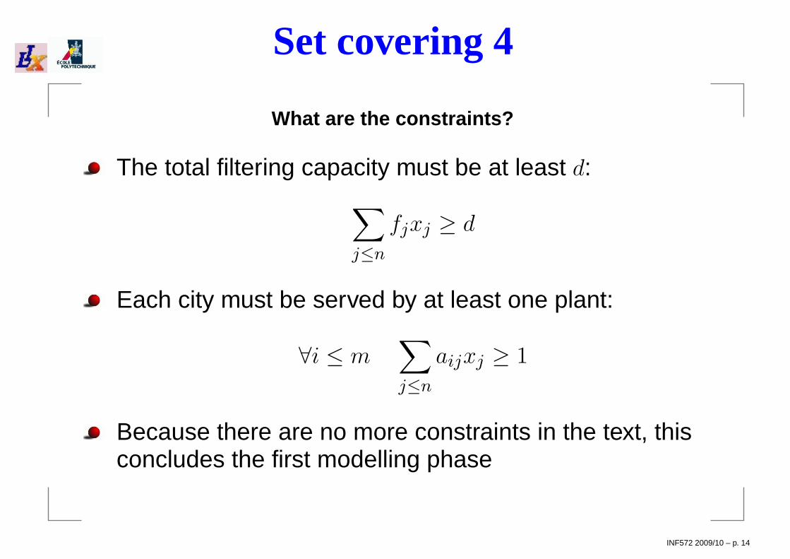
An elementary run file

Consider the set covering problem, suppose we havecoded the model file (setcovering.mod ) and the datafile (setcovering.dat ), and that the CPLEX solver isinstalled on the system

Then the following is a basic setcovering.run file

# basic run file for setcovering problemmodel setcovering.mod; # specify model filedata setcovering.dat; # specify data fileoption solver cplex; # specify solversolve; # solve the problemdisplay cost; # display opt. costdisplay x; # display opt. soln.

INF572 2009/10 – p. 20

Set covering model file# setcovering.mod

param m integer, >= 0;

param n integer, >= 0;

set M := 1..m;

set N := 1..n;

param cN >= 0;

param aM,N binary;

param fN >= 0;

param d >= 0;

var xj in N binary;

minimize cost: sumj in N c[j] * x[j];

subject to capacity: sumj in N f[j] * x[j] >= d;

subject to coveringi in M: sumj in N a[i,j] * x[j] >= 1;

INF572 2009/10 – p. 21

Set covering data fileparam m := 5;

param n := 12;

param : c f :=

1 7 15

2 9 39

3 12 26

4 3 31

5 4 34

6 4 24

7 5 51

8 11 19

9 8 18

10 6 36

11 7 41

12 16 34 ;

param a: 1 2 3 4 5 6 7 8 9 10 11 12 :=

1 1 0 1 0 1 0 1 1 0 0 0 0

2 0 1 1 0 0 1 0 0 1 0 1 1

3 1 1 0 0 0 1 1 0 0 1 0 0

4 0 1 0 1 0 0 1 1 0 1 0 1

5 0 0 0 1 1 1 0 0 1 1 1 1 ;

param d := 120; INF572 2009/10 – p. 22

AMPL+CPLEX solutionliberti@nox$ cat setcovering.run | ampl

ILOG CPLEX 11.010, options: e m b q use=2

CPLEX 11.0.1: optimal integer solution; objective 15

3 MIP simplex iterations

0 branch-and-bound nodes

cost = 15

x [ * ] :=

1 0

2 0

3 0

4 1

5 0

6 0

7 1

8 0

9 0

10 0

11 1

12 0

;

INF572 2009/10 – p. 23

AMPL Grammar

INF572 2009/10 – p. 24

AMPL MP LanguageThere are 5 main entities: sets, parameters, variables, objectives andconstraints

In AMPL, each entity has a name and can be quantified

set name [quantifier] attributes ;

param name [quantifier] attributes ;

var name [quantifier] attributes ;

minimize | maximize name [quantifier]: iexpr ;

subject to name [quantifier]: iexpr <= | = | >= iexpr ;

Attributes on sets and parameters is used to validate values readfrom data files

Attributes on vars specify integrality (binary , integer ) and limitconstraints (>= lower , <= upper )

Entities indices: square brackets (e.g. y[1] , x[i,k] )

The above is the basic syntax — there are some advanced options

INF572 2009/10 – p. 25

AMPL data specification

In general, syntax is in map-like form; a

param p i in S integer;

is a map S → Z, and each pair (domain, codomain) must bespecified:

param p :=1 42 -33 0;

The grammar is simple but tedious, best way islearning by example or trial and error

INF572 2009/10 – p. 26

AMPL imperative languagemodel model filename.mod ;

data data filename.dat ;

option option name literal string, ... ;

solve ;

display [quantifier] iexpr ; / printf (syntax similar to C)

let [quantifier] ivar := number;

if ( condition list) then commands [else commands]for quantifier commands / break; / continue;

shell ’ command line’; / exit number; / quit;

cd dir name; / remove file name;

In all output commands, screen output can be redirected to a file byappending > output filename.txt before the semicolon

These are basic commands, there are some advanced ones

INF572 2009/10 – p. 27

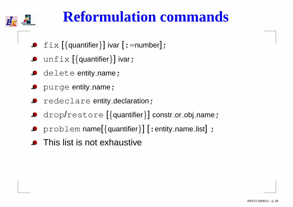
Reformulation commands

fix [quantifier] ivar [:= number];

unfix [quantifier] ivar;

delete entity name;

purge entity name;

redeclare entity declaration;

drop /restore [quantifier] constr or obj name;

problem name[quantifier] [: entity name list] ;

This list is not exhaustive

INF572 2009/10 – p. 28

Solvers

INF572 2009/10 – p. 29

SolversIn order of solver reliability / effectiveness:

1. LPs : use an LP solver (O(106) vars/constrs, fast, e.g. CPLEX, CLP,GLPK)

2. MILPs : use a MILP solver (O(104) vars/constrs, can be slow,e.g. CPLEX, Symphony, GLPK)

3. NLPs : use a local NLP solver to get a local optimum (O(104)

vars/constrs, quite fast, e.g. SNOPT, MINOS, IPOPT)

4. NLPs/MINLPs : use a heuristic solver to get a good local optimum(O(103), quite fast, e.g. BONMIN, MINLP_BB)

5. NLPs : use a global NLP solver to get an (approximated) globaloptimum (O(103) vars/constrs, can be slow, e.g. COUENNE, BARON)

6. MINLPs : use a global MINLP solver to get an (approximated) globaloptimum (O(103) vars/constrs, can be slow, e.g. COUENNE, BARON)

Not all these solvers are available via AMPL

INF572 2009/10 – p. 30

Solution algorithms (linear)

LPs : (convex)

1. simplex algorithm (non-polynomial complexity butvery fast in practice, reliable)

2. interior point algorithms (polynomial complexity,quite fast, fairly reliable)

MILPs : (nonconvex because of integrality)

1. Local (heuristics): Local Branching, Feasibility Pump[Fischetti&Lodi 05], VNS [Hansen et al. 06] (quitefast, reliable)

2. Global: Branch-and-Bound (exact algorithm,non-polynomial complexity but often quite fast,heuristic if early termination, reliable)

INF572 2009/10 – p. 31

Solution algorithms (nonlinear)

NLPs : (may be convex or nonconvex)

1. Local: Sequential Linear Programming (SLP), SequentialQuadratic Programming (SQP), interior point methods(linear/polynomial convergence, often quite fast, unreliable)

2. Global: spatial Branch-and-Bound [Smith&Pantelides 99](ε-approximate, nonpolynomial complexity, often quite slow,heuristic if early termination, unreliable)

MINLPs : (nonconvex because of integrality and terms)

1. Local (heuristics): Branching explorations [Fletcher&Leyffer 99],Outer approximation [Grossmann 86], Feasibility pump [Bonamiet al. 06] (nonpolynomial complexity, often quite fast, unreliable)

2. Global: spatial Branch-and-Bound [Sahinidis&Tawarmalani 05](ε-approximate, nonpolynomial complexity, often quite slow,heuristic if early termination, unreliable)

INF572 2009/10 – p. 32

Canonical MP formulation

minx f(x)

s.t. l ≤ g(x) ≤ u

xL ≤ x ≤ xU

∀i ∈ Z ⊆ 1, . . . , n xi ∈ Z

[P ] (1)

where x, xL, xU ∈ Rn; l, u ∈ Rm; f : Rn → R; g : Rn → Rm

A point x∗ is feasible in P if l ≤ g(x∗) ≤ u, xL ≤ x∗ ≤ xU and∀i ∈ Z (x∗

i ∈ Z); F (P ) = set of feasible points of P

If gi(x∗) = l or = u for some i, gi is active at x∗

A feasible x∗ is a local minimum if ∃B(x∗, ε) s.t. ∀x ∈ F (P ) ∩B(x∗, ε)

we have f(x∗) ≤ f(x)

A feasible x∗ is a global minimum if ∀x ∈ F (P ) we have f(x∗) ≤ f(x)

INF572 2009/10 – p. 33

Feasibility and optimality

F (P ) = feasible region of P , L(P ) = set of local optima,G(P ) = set of global optima

Nonconvexity⇒ G(P ) ( L(P )

minx∈[−3,6]

14x + sin(x) −3

60 x

INF572 2009/10 – p. 34

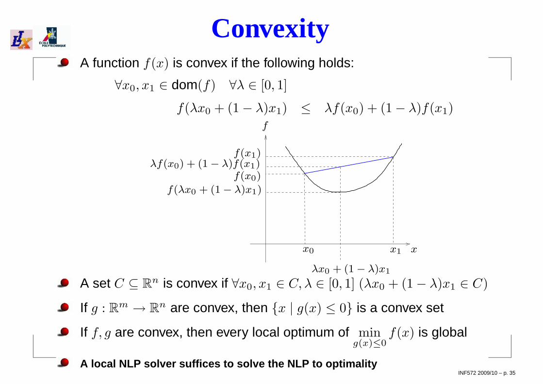
ConvexityA function f(x) is convex if the following holds:

∀x0, x1 ∈ dom(f) ∀λ ∈ [0, 1]

f(λx0 + (1− λ)x1) ≤ λf(x0) + (1− λ)f(x1)

x

f

x0 x1

f(x0)

f(x1)

λx0 + (1 − λ)x1

f(λx0 + (1 − λ)x1)

λf(x0) + (1 − λ)f(x1)

A set C ⊆ Rn is convex if ∀x0, x1 ∈ C, λ ∈ [0, 1] (λx0 + (1− λ)x1 ∈ C)

If g : Rm → Rn are convex, then x | g(x) ≤ 0 is a convex set

If f, g are convex, then every local optimum of ming(x)≤0

f(x) is global

A local NLP solver suffices to solve the NLP to optimalityINF572 2009/10 – p. 35

Canonical form

P is a linear programming problem (LP) if f : Rn → R,g : Rn → Rm are linear forms

LP in canonical form:

minx cTx

s.t. Ax ≤ b

x ≥ 0

[C] (2)

Can reformulate inequalities to equations by adding anon-negative slack variable xn+1 ≥ 0:

n∑

j=1

ajxj ≤ b ⇒n∑

j=1

ajxj + xn+1 = b ∧ xn+1 ≥ 0

INF572 2009/10 – p. 36

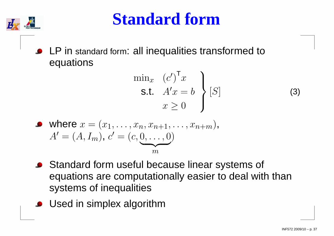
Standard form

LP in standard form: all inequalities transformed toequations

minx (c′)Tx

s.t. A′x = b

x ≥ 0

[S] (3)

where x = (x1, . . . , xn, xn+1, . . . , xn+m),A′ = (A, Im), c′ = (c, 0, . . . , 0

︸ ︷︷ ︸

m

)

Standard form useful because linear systems ofequations are computationally easier to deal with thansystems of inequalities

Used in simplex algorithm

INF572 2009/10 – p. 37

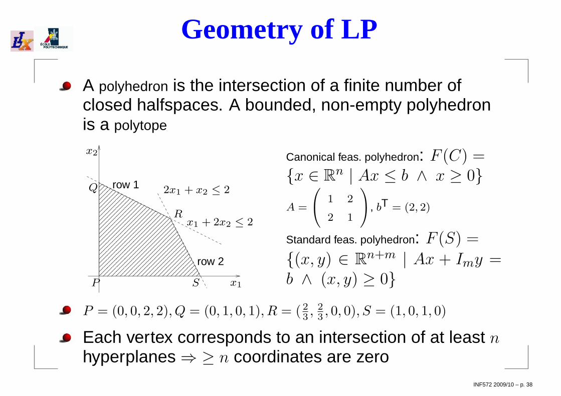
Geometry of LP

A polyhedron is the intersection of a finite number ofclosed halfspaces. A bounded, non-empty polyhedronis a polytope

x1

x2

x1 + 2x2 ≤ 2

2x1 + x2 ≤ 2

P

Q

R

S

row 1

row 2

Canonical feas. polyhedron: F (C) =x ∈ Rn | Ax ≤ b ∧ x ≥ 0A =

0

@

1 2

2 1

1

A, bT = (2, 2)

Standard feas. polyhedron: F (S) =

(x, y) ∈ Rn+m | Ax + Imy =b ∧ (x, y) ≥ 0

P = (0, 0, 2, 2), Q = (0, 1, 0, 1), R = (23 , 2

3 , 0, 0), S = (1, 0, 1, 0)

Each vertex corresponds to an intersection of at least nhyperplanes⇒ ≥ n coordinates are zero

INF572 2009/10 – p. 38

Basic feasible solutions

Consider polyhedron in “equation form”K = x ∈ Rn | Ax = b ∧ x ≥ 0. A is m× n of rank m(N.B. n here is like n + m in last slide!)

A subset of m linearly independent columns of A is abasis of A

If β is the set of column indices of a basis of A,variables xi are basic for i ∈ β and nonbasic for i 6∈ β

Partition A in a square m×m nonsingular matrix B(columns indexed by β) and an (n−m)×m matrix N

Write A = (B|N), xB ∈ Rm basics, xN ∈ Rn−m nonbasics

Given a basis (B|N) of A, the vector x = (xB, xN ) is abasic feasible solution (bfs) of K with respect to the givenbasis if Ax = b, xB ≥ 0 and xN = 0

INF572 2009/10 – p. 39

Fundamental Theorem of LP

Given a non-empty polyhedron K in “equation form”,there is a surjective mapping between bfs and verticesof K

For any c ∈ Rn, either there is at least one bfs thatsolves the LP mincTx |x ∈ K, or the problem isunbounded

Proofs not difficult but long (see lecture notes orPapadimitriou and Steiglitz)

Important correspondence between bfs’s and verticessuggests geometric solution method based on exploringvertices of K

INF572 2009/10 – p. 40

Simplex Algorithm: Summary

Solves LPs in form minx∈K

cTx where K = Ax = b ∧ x ≥ 0

Starts from any vertex x

Moves to an adjacent improving vertex x′

(i.e. x′ is s.t. ∃ edge x, x′ in K and cTx′ ≤ cTx)

Two bfs’s with basic vars indexed by sets β, β′

correspond to adjacent vertices if |β ∩ β′| = m− 1

Stops when no such x′ exists

Detects unboundedness and prevents cycling⇒convergence

K convex⇒ global optimality follows from localoptimality at termination

INF572 2009/10 – p. 41

Simplex Algorithm I

Let x = (x1, . . . , xn) be the current bfs, write Ax = b asBxB + NxN = b

Express basics in terms of nonbasics:xB = B−1b−B−1NxN (this system is a dictionary)

Express objective function in terms of nonbasics:cTx = cT

BxB + cTNxN = cT

B(B−1b−B−1NxN ) + cTNxN ⇒

⇒ cTx = cTBB−1b + cT

NxN

(cTN = cT

N − cTBB−1N are the reduced costs)

Select an improving direction: choose a nonbasicvariable xh with negative reduced cost; increasing itsvalue will decrease the objective function value

If no such h exists, no improving direction, localminimum⇒ global minimum⇒ termination

INF572 2009/10 – p. 42

Simplex Algorithm II

Iteration start: xh is out of basis⇒ its value is zero

We want to increase its value to strictly positive todecrease objective function value

. . . corresponds to “moving along an edge”

We stop when we reach another (improving) vertex

. . . corresponds to setting a basic variable xl to zero

x1

x2

P

Q

R: optimum

S

P = (0, 0, 2, 2)

row 2

increase x1

x1

x2

P

Q

R: optimum

S

row 1

S = (1, 0, 1, 0)

x1 enters, x4 exits

xh enters the basis, xl exits the basisINF572 2009/10 – p. 43

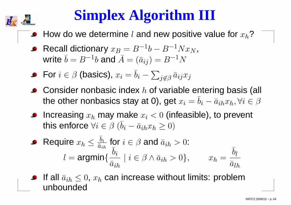
Simplex Algorithm IIIHow do we determine l and new positive value for xh?

Recall dictionary xB = B−1b−B−1NxN ,write b = B−1b and A = (aij) = B−1N

For i ∈ β (basics), xi = bi −∑

j 6∈β aijxj

Consider nonbasic index h of variable entering basis (allthe other nonbasics stay at 0), get xi = bi − aihxh,∀i ∈ β

Increasing xh may make xi < 0 (infeasible), to preventthis enforce ∀i ∈ β (bi − aihxh ≥ 0)

Require xh ≤ bi

aihfor i ∈ β and aih > 0:

l = argmin bi

aih| i ∈ β ∧ aih > 0, xh =

bl

alh

If all aih ≤ 0, xh can increase without limits: problemunbounded

INF572 2009/10 – p. 44

Simplex Algorithm IV

Suppose > n hyperplanes cross at vtx R (degenerate)

May get improving direction s.t. adjacent vertex is still R

Objective function value does not change

Seq. of improving dirs. may fail to move away from R

⇒ simplex algorithm cycles indefinitely

Use Bland’s rule: among candidate entering / exitingvariables, choose that with least index

x1

x2

x1 + 2x2 ≤ 2

2x1 + x2 ≤ 2

3x1 + 3x2 ≤ 4

P

Q

R: crossing of three lines

S

INF572 2009/10 – p. 45

Example: FormulationConsider problem:

maxx1,x2

x1 + x2

s.t. x1 + 2x2 ≤ 2

2x1 + x2 ≤ 2

x ≥ 0

Standard form:

−minx −x1 − x2

s.t. x1 + 2x2 + x3 = 2

2x1 + x2 + x4 = 2

x ≥ 0

Obj. fun.: max f = −min−f , simply solve for min−fINF572 2009/10 – p. 46

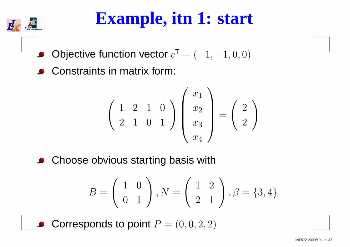
Example, itn 1: start

Objective function vector cT = (−1,−1, 0, 0)

Constraints in matrix form:

(

1 2 1 0

2 1 0 1

)

x1

x2

x3

x4

=

(

2

2

)

Choose obvious starting basis with

B =

(

1 0

0 1

)

, N =

(

1 2

2 1

)

, β = 3, 4

Corresponds to point P = (0, 0, 2, 2)

INF572 2009/10 – p. 47

Example, itn 1: dictionary

Start the simplex algorithm with basis in P

row 1

row 2

x1

x2

x1 + 2x2 ≤ 2

2x1 + x2 ≤ 2

P

Q

R

S

−∇f

Compute dictionary xB = B−1b−B−1NxN = b− AxN ,where

b =

(

2

2

)

; A =

(

1 2

2 1

)

INF572 2009/10 – p. 48

Example, itn 1: entering var

Compute reduced costs cN = cTN − cT

BA:

(c1, c2) = (−1,−1)− (0, 0)A = (−1,−1)

All nonbasic variables x1, x2 have negative reducedcost, can choose whichever to enter the basis

Bland’s rule: choose entering nonbasic with least indexin x1, x2, i.e. pick h = 1 (move along edge PS)

row 1

row 2

x1

x2

x1 + 2x2 ≤ 2

2x1 + x2 ≤ 2

P

Q

R

S

−∇f

x1 enters the basisINF572 2009/10 – p. 49

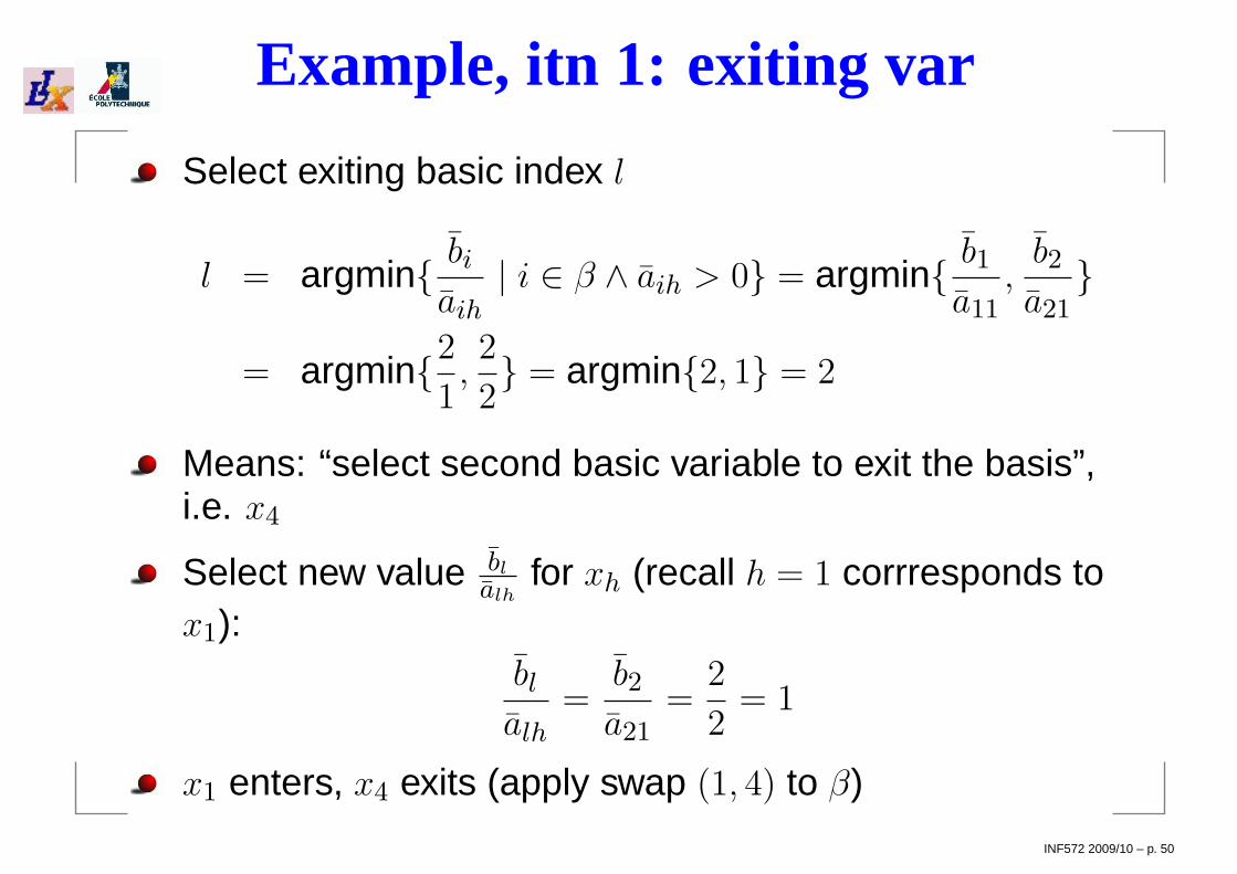
Example, itn 1: exiting var

Select exiting basic index l

l = argmin bi

aih| i ∈ β ∧ aih > 0 = argmin b1

a11,

b2

a21

= argmin21,2

2 = argmin2, 1 = 2

Means: “select second basic variable to exit the basis”,i.e. x4

Select new value bl

alhfor xh (recall h = 1 corrresponds to

x1):bl

alh=

b2

a21=

2

2= 1

x1 enters, x4 exits (apply swap (1, 4) to β)

INF572 2009/10 – p. 50

Example, itn 2: start

Start of new iteration: basis is β = 1, 3

B =

(

1 1

2 0

)

; B−1 =

(

0 12

1 −12

)

xB = (x1, x3) = B−1b = (1, 1), thus current bfs is(1, 0, 1, 0) = S

row 1

row 2

x1

x2

x1 + 2x2 ≤ 2

2x1 + x2 ≤ 2

P

Q

R

S

−∇f

INF572 2009/10 – p. 51

Example, itn 2: entering var

Compute dictionary: b = B−1b = (1, 1)T,

A = B−1N =

(

0 12

1 −12

)(

2 0

1 1

)

=

(12

12

32 −1

2

)

Compute reduced costs:(c2, c4) = (−1, 0)− (−1, 0)A = (−1/2, 1/2)

Pick h = 1 (corresponds to x2 entering the basis)

row 1

x1

x2

x1 + 2x2 ≤ 2

2x1 + x2 ≤ 2

P

Q

R

S

x2 enters basis

−∇f

INF572 2009/10 – p. 52

Example, itn 2: exiting var

Compute l and new value for x2:

l = argmin b1

a11,

b2

a21 = argmin 1

1/2,

1

3/2 =

= argmin2, 2/3 = 2

l = 2 corresponds to second basic variable x3

New value for x2 entering basis: 23

x2 enters, x3 exits (apply swap (2, 3) to β)

INF572 2009/10 – p. 53

Example, itn 3: start

Start of new iteration: basis is β = 1, 2

B =

(

1 2

2 1

)

; B−1 =

(

−13

23

23 −1

3

)

xB = (x1, x2) = B−1b = (23 , 2

3), thus current bfs is(23 , 2

3 , 0, 0) = R

row 1

row 2

x1

x2

x1 + 2x2 ≤ 2

2x1 + x2 ≤ 2

P

Q

R

S

−∇f

INF572 2009/10 – p. 54

Example, itn 3: termination

Compute dictionary: b = B−1b = (2/3, 2/3)T,

A = B−1N =

(

−13

23

23 −1

3

)(

1 0

0 1

)

=

(

−13

23

23 −1

3

)

Compute reduced costs:(c3, c4) = (0, 0)− (−1,−1)A = (1/3, 1/3)

No negative reduced cost: algorithm terminates

Optimal basis: 1, 2Optimal solution: R = (2

3 , 23)

Optimal objective function value f(R) = −43

Permutation to apply to initial basis 3, 4: (1, 4)(2, 3)

INF572 2009/10 – p. 55

Interior point methodsSimplex algorithm is practically efficient but nobody everfound a pivot choice rule that proves that it haspolynomial worst-case running time

Nobody ever managed to prove that such a rule doesnot exist

With current pivoting rules, simplex worst-case runningtime is exponential

Kachiyan managed to prove in 1979 that LP ∈ P using apolynomial algorithm called ellipsoid method(http://www.stanford.edu/class/msande310/ellip.pdf )

Ellipsoid method has polynomial worst-case runningtime but performs badly in practice

Barrier interior point methods for LP have bothpolynomial running time and good practicalperformances

INF572 2009/10 – p. 56

IPM I: Preliminaries

Consider LP P in standard form:mincTx | Ax = b ∧ x ≥ 0.Reformulate by introducing “logarithmic barriers”:

P (β) : mincTx− β

n∑

j=1

log xj | Ax = b

−β log(x)

x

decreasing β

The term −β log(xj) is a“penalty” that ensures thatxj > 0; the “limit” of thisreformulation for β → 0 shouldensure that xj ≥ 0 as desired

Notice P (β) is convex ∀β > 0

INF572 2009/10 – p. 57

IPM II: Central path

Let x∗(β) the optimal solution of P (β) and x∗ the optimalsolution of P

The set x∗(β) | β > 0 is called the central path

Idea: determine the central path bysolving a sequence of convexproblems P (β) for some decreasingsequence of values of β and showthat x∗(β)→ x∗ as β → 0

Since for β > 0, −β log(xj) → +∞for xj → 0, x∗(β) will never be on theboundary of the feasible polyhedronx ≥ 0 | Ax = b; thus the name “inte-rior point method”

0 0.5 1 1.5 2 2.5 30

0.2

0.4

0.6

0.8

1

1.2

1.4

1.6

1.8

2

INF572 2009/10 – p. 58

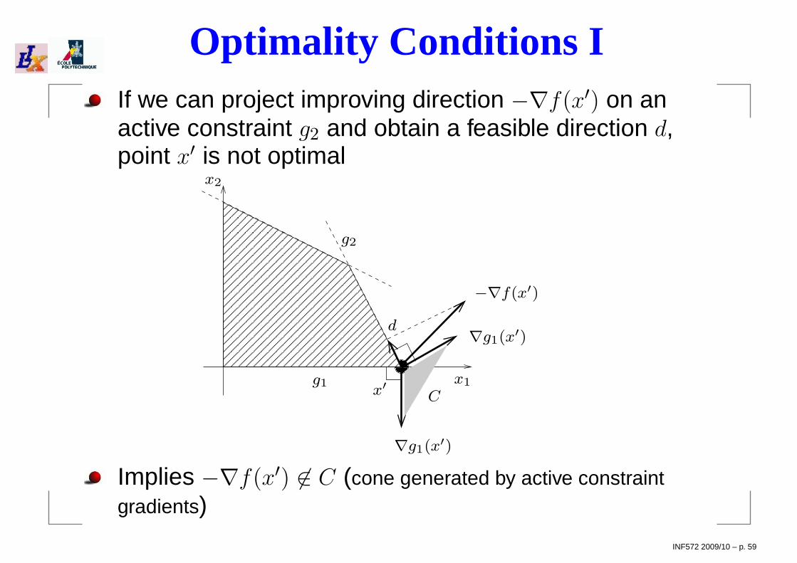
Optimality Conditions IIf we can project improving direction −∇f(x′) on anactive constraint g2 and obtain a feasible direction d,point x′ is not optimal

x1

x2

x′g1

g2

∇g1(x′)

∇g1(x′)

−∇f(x′)

C

d

Implies −∇f(x′) 6∈ C (cone generated by active constraintgradients)

INF572 2009/10 – p. 59

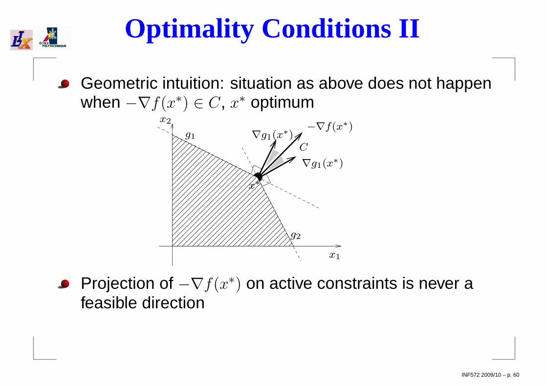
Optimality Conditions II

Geometric intuition: situation as above does not happenwhen −∇f(x∗) ∈ C, x∗ optimum

x1

x2

x∗

g1

g2

∇g1(x∗)

∇g1(x∗)

−∇f(x∗)

C

Projection of −∇f(x∗) on active constraints is never afeasible direction

INF572 2009/10 – p. 60

Optimality Conditions III

If:1. x∗ is a local minimum of problem

P ≡ minf(x) | g(x) ≤ 0,2. I is the index set of the active constraints at x∗,

i.e. ∀i ∈ I (gi(x∗) = 0)

3. ∇gI(x∗) = ∇gi(x

∗) | i ∈ I is a linearly independentset of vectors

then −∇f(x∗) is a conic combination of ∇gI(x∗),

i.e. ∃y ∈ R|I| such that

∇f(x∗) +∑

i∈I

yi∇gi(x∗) = 0

∀i ∈ I yi ≥ 0

INF572 2009/10 – p. 61

Karush-Kuhn-Tucker Conditions

Define

L(x, y) = f(x) +m∑

i=1

yigi(x)

as the Lagrangian of problem P

KKT: If x∗ is a local minimum of problem P and ∇g(x∗)is a linearly independent set of vectors, ∃y ∈ Rm s.t.

∇x∗L(x, y) = 0

∀i ≤ m (yigi(x∗) = 0)

∀i ≤ m (yi ≥ 0)

INF572 2009/10 – p. 62

Weak dualityThm.Let L(y) = min

x∈F (P )L(x, y) and x∗ be the global optimum

of P . Then ∀y ≥ 0 L(y) ≤ f(x∗).

ProofSince y ≥ 0, if x ∈ F (P ) then yigi(x) ≤ 0, henceL(x, y) ≤ f(x); result follows as we are taking the mini-mum over all x ∈ F (P ).

Important point: L(y) is a lower bound for P for all y ≥ 0

The problem of finding the tightest Lagrangian lowerbound

maxy≥0

minx∈F (P )

L(x, y)

is the Lagrangian dual of problem P

INF572 2009/10 – p. 63

Dual of an LP I

Consider LP P in form: mincTx | Ax ≥ b ∧ x ≥ 0L(x, s, y) = cTx− sTx + yT(b− Ax) where s ∈ Rn, y ∈ Rm

Lagrangian dual:

maxs,y≥0

minx∈F (P )

(yb + (cT − s− yA)x)

KKT: for a point x to be optimal,

cT − s− yA = 0 (KKT1)∀j ≤ n (sjxj = 0), ∀i ≤ m (yi(bi − Aix) = 0) (KKT2)

s, y ≥ 0 (KKT3)

Consider Lagrangian dual s.t. (KKT1), (KKT3):

INF572 2009/10 – p. 64

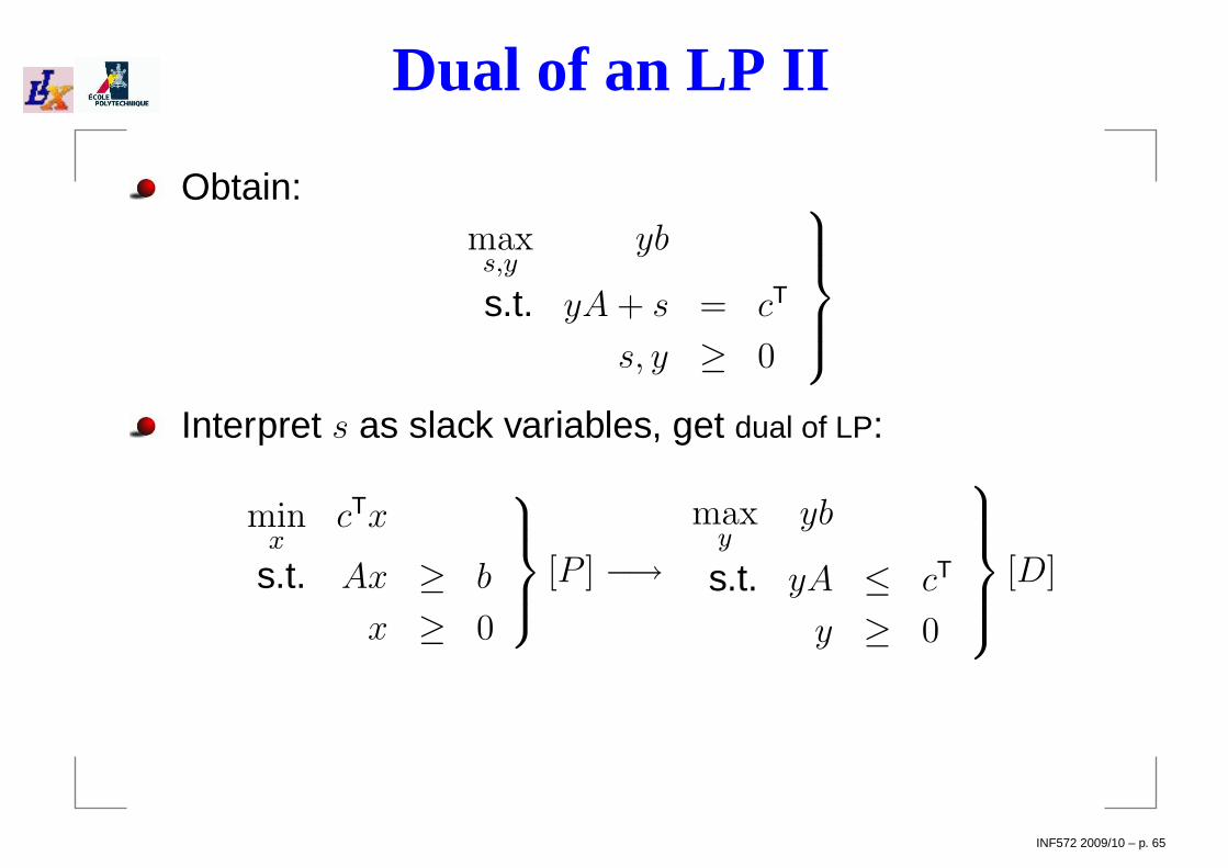
Dual of an LP II

Obtain:maxs,y

yb

s.t. yA + s = cT

s, y ≥ 0

Interpret s as slack variables, get dual of LP:

minx

cTx

s.t. Ax ≥ b

x ≥ 0

[P ] −→max

yyb

s.t. yA ≤ cT

y ≥ 0

[D]

INF572 2009/10 – p. 65

Alternative derivation of LP dual

Lagrangian dual⇒ find tightest lower bound for LPmin cTx s.t. Ax ≥ b and x ≥ 0

Multiply constraints Ax ≥ b by coefficients y1, . . . , ym toobtain the inequalities yiAx ≥ yib, valid provided y ≥ 0

Sum over i:∑

i yiAx ≥∑i yib = yAx ≥ yb

Look for y such that obtained inequalities are asstringent as possible whilst still a lower bound for cTx

⇒ yb ≤ yAx and yb ≤ cTx

Suggests setting yA = cT and maximizing yb

Obtain LP dual: max yb s.t. yA = cT and y ≥ 0.

INF572 2009/10 – p. 66

Strong Duality for LP

Thm.If x is optimum of a linear problem and y is the optimumof its dual, primal and dual objective functions attain thesame values at x and respectively y.Proof

Assume x optimum, KKT conditions hold

Recall (KKT2) ∀j ≤ n(sixi = 0),∀i ≤ m (yi(bi − Aix) = 0)

Get y(b− Ax) = sx⇒ yb = (yA + s)x

By (KKT1) yA + s = cT

Obtain yb = cTx

INF572 2009/10 – p. 67

Strong Duality for convex NLPs ITheory of KKT conditions derived for generic NLPmin f(x) s.t. g(x) ≤ 0, independent of linearity of f, g

Derive strong duality results for convex NLPs

Slater condition ∃x′ ∈ F (P ) (g(x′) < 0) requiresnon-empty interior of F (P )

Let f∗ = minx:g(x)≤0 f(x) be the optimal objectivefunction value of the primal problem P

Let p∗ = maxy≥0 minx∈F (P ) L(x, y) be the optimalobjective function value of the Lagrangian dual

Thm.If f, g are convex functions and Slater’s condition holds,then f∗ = p∗.

INF572 2009/10 – p. 68

Strong Duality for convex NLPs IIProof- Let A = (λ, t) | ∃x (λ ≥ g(x) ∧ t ≥ f(x)), B = (0, t) | t < f∗

- A =set of values taken byconstraints and objectives

- A ∩ B = ∅ for otherwise f∗ notoptimal

- P is convex⇒ A,B convex

- ⇒ ∃ separating hyperplaneuλ + µt = α s.t.

∀(λ, t) ∈ A (uλ + µt ≥ α) (4)

∀(λ, t) ∈ B (uλ + µt ≤ α) (5)

- Since λ, t may increase indefinitely, (4) bounded below⇒ u ≥ 0, µ ≥ 0

INF572 2009/10 – p. 69

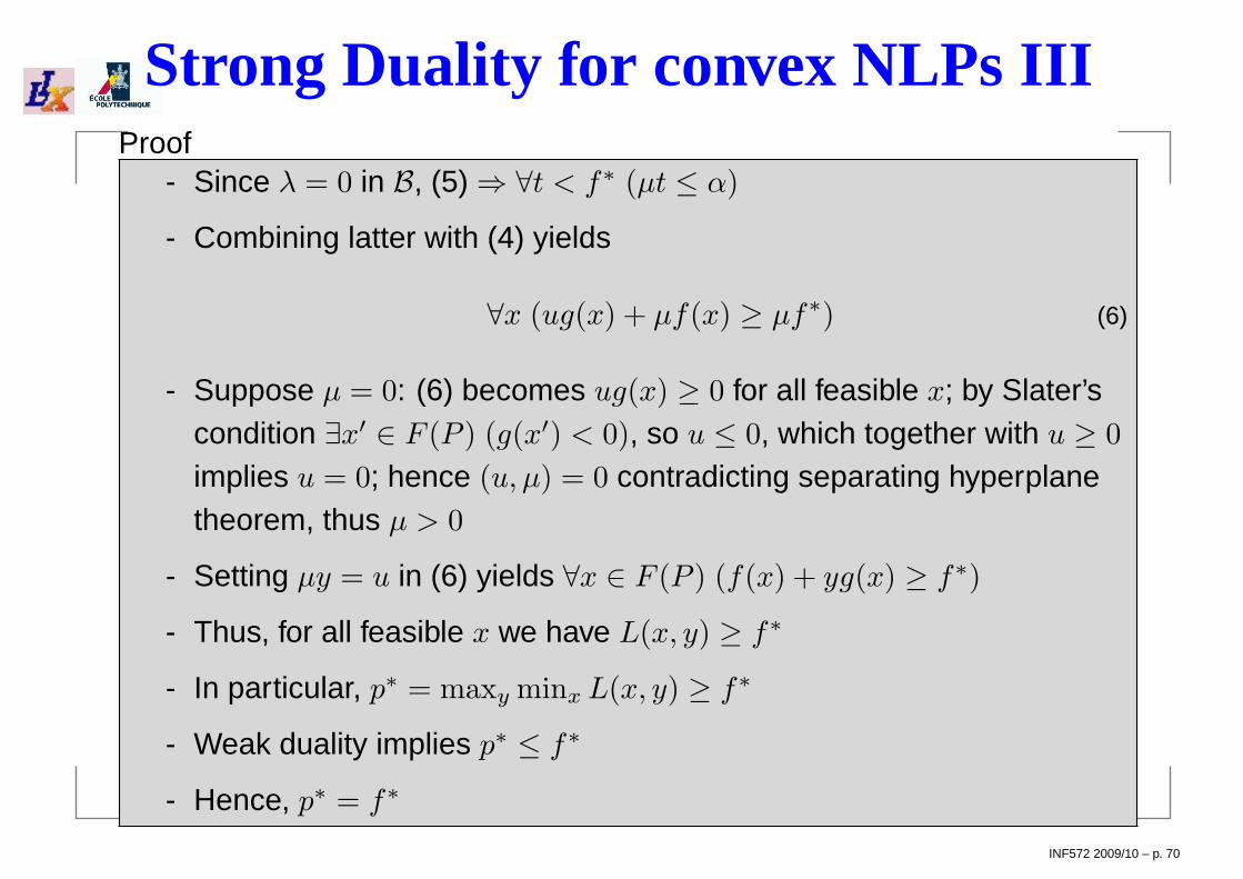
Strong Duality for convex NLPs IIIProof

- Since λ = 0 in B, (5)⇒ ∀t < f∗ (µt ≤ α)

- Combining latter with (4) yields

∀x (ug(x) + µf(x) ≥ µf∗) (6)

- Suppose µ = 0: (6) becomes ug(x) ≥ 0 for all feasible x; by Slater’scondition ∃x′ ∈ F (P ) (g(x′) < 0), so u ≤ 0, which together with u ≥ 0

implies u = 0; hence (u, µ) = 0 contradicting separating hyperplanetheorem, thus µ > 0

- Setting µy = u in (6) yields ∀x ∈ F (P ) (f(x) + yg(x) ≥ f∗)

- Thus, for all feasible x we have L(x, y) ≥ f∗

- In particular, p∗ = maxy minx L(x, y) ≥ f∗

- Weak duality implies p∗ ≤ f∗

- Hence, p∗ = f∗

INF572 2009/10 – p. 70

Rules for LP dualPrimal Dual

min max

variables x constraints

constraints variables y

objective coefficients c constraint right hand sides c

constraint right hand sides b objective coefficients b

Aix ≥ bi yi ≥ 0

Aix ≤ bi yi ≤ 0

Aix = bi yi unconstrainedxj ≥ 0 yAj ≤ cj

xj ≤ 0 yAj ≥ cj

xj unconstrained yAj = cj

Ai: i-th row of A Aj : j-th column of AINF572 2009/10 – p. 71

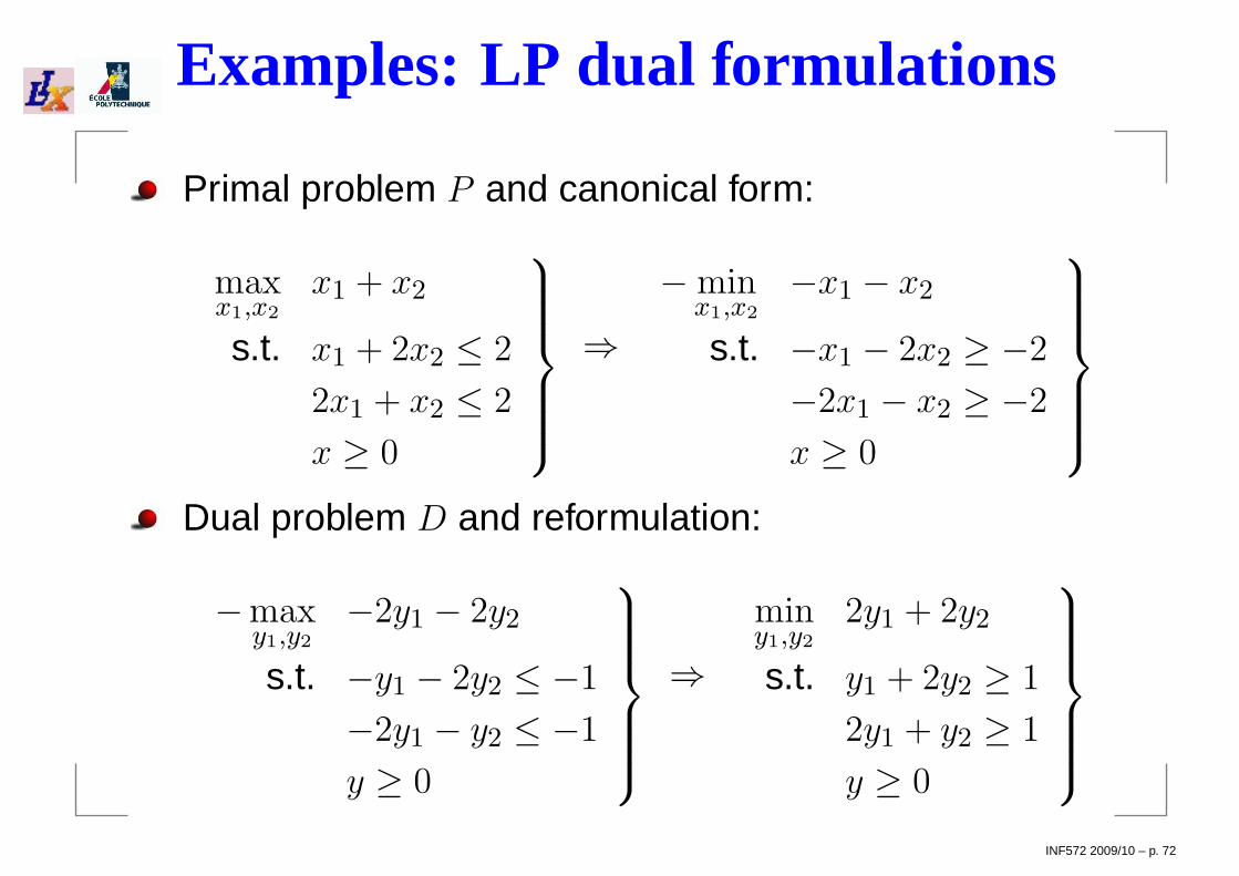
Examples: LP dual formulations

Primal problem P and canonical form:

maxx1,x2

x1 + x2

s.t. x1 + 2x2 ≤ 2

2x1 + x2 ≤ 2

x ≥ 0

⇒−min

x1,x2

−x1 − x2

s.t. −x1 − 2x2 ≥ −2

−2x1 − x2 ≥ −2

x ≥ 0

Dual problem D and reformulation:

−maxy1,y2

−2y1 − 2y2

s.t. −y1 − 2y2 ≤ −1

−2y1 − y2 ≤ −1

y ≥ 0

⇒miny1,y2

2y1 + 2y2

s.t. y1 + 2y2 ≥ 1

2y1 + y2 ≥ 1

y ≥ 0

INF572 2009/10 – p. 72

Example: Shortest Path ProblemSHORTEST PATH PROBLEM.Input: weighted digraph G =(V,A, c), and s, t ∈ V .Output: a minimum-weight pathin G from s to t. 1

2

2

2

6

41

11

1

5

0

3

s

t

minx≥0

∑

(u,v)∈A

cuvxuv

∀ v ∈ V∑

(v,u)∈A

xvu −∑

(u,v)∈A

xuv =

1 v = s

−1 v = t

0 othw.

[P ]

maxy

ys − yt

∀ (u, v) ∈ A yv − yu ≤ cuv

[D]

INF572 2009/10 – p. 73

Shortest Path Dual

2

2

4

1

2

3

4

cols (1,2) (1,3) . . . (4,1) . . .rows\c 2 2 . . . 4 . . . b

1 1 1 . . . -1 . . . 0 y1

2 -1 0 . . . 0 . . . 0 y2

3 0 -1 . . . 0 . . . 0 y3

4 0 0 . . . 1 . . . 0 y4...

......

......

...s 0 0 . . . 0 . . . 1 ys

......

......

......

t 0 0 . . . 0 . . . -1 yt

......

......

......

x12 x13 . . . x41 . . .

INF572 2009/10 – p. 74

SP Mechanical Algorithm

12

3

ysytmin yt max ys

st

≤ c13

1 2

3

ysyt

st= c1t

= c21 = cs2

xuv = 1

KKT2 on [D] ⇒ ∀(u, v) ∈ A (xuv(yv − yu − cuv) = 0)⇒∀(u, v) ∈ A (xuv = 1→ yv − yu = cuv)

INF572 2009/10 – p. 75

exAMPLes

INF572 2009/10 – p. 76

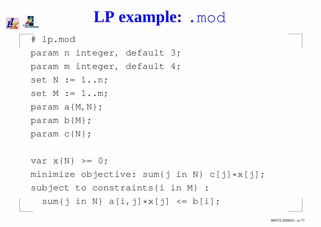
LP example: .mod# lp.mod

param n integer, default 3;

param m integer, default 4;

set N := 1..n;

set M := 1..m;

param aM,N;

param bM;

param cN;

var xN >= 0;

minimize objective: sumj in N c[j] * x[j];

subject to constraintsi in M :

sumj in N a[i,j] * x[j] <= b[i];

INF572 2009/10 – p. 77

LP example: .dat# lp.dat

param n := 3; param m := 4;

param c :=

1 1

2 -3

3 -2.2 ;

param b :=

1 -1

2 1.1

3 2.4

4 0.8 ;

param a : 1 2 3 :=

1 0.1 0 -3.1

2 2.7 -5.2 1.3

3 1 0 -1

4 1 1 0 ;

INF572 2009/10 – p. 78

LP example: .run

# lp.run

model lp.mod;data lp.dat;option solver cplex;solve;display x;

INF572 2009/10 – p. 79

LP example: output

CPLEX 11.0.1: optimal solution; objective -11.301538460 dual simplex iterations (0 in phase I)x [ * ] :=1 02 0.83 4.04615;

INF572 2009/10 – p. 80

MILP example: .mod# milp.mod

param n integer, default 3;

param m integer, default 4;

set N := 1..n;

set M := 1..m;

param aM,N;

param bM;

param cN;

var xN >= 0, <= 3, integer;

var y >= 0;

minimize objective: sumj in N c[j] * x[j];

subject to constraintsi in M :

sumj in N a[i,j] * x[j] - y <= b[i];INF572 2009/10 – p. 81

MILP example: .run

# milp.run

model milp.mod;data lp.dat;option solver cplex;solve;display x;display y;

INF572 2009/10 – p. 82

MILP example: output

CPLEX 11.0.1: optimal integer solution; objective -15.60 MIP simplex iterations0 branch-and-bound nodesx [ * ] :=1 02 33 3;y = 2.2

INF572 2009/10 – p. 83

NLP example: .mod

# nlp.mod

param n integer, default 3;

param m integer, default 4;

set N := 1..n;

set M := 1..m;

param aM,N;

param bM;

param cN;

var xN >= 0.1, <= 4;

minimize objective:

c[1] * x[1] * x[2] + c[2] * x[3]ˆ2 + c[3] * x[1] * x[2]/x[3];

subject to constraintsi in M diff 4 :

sumj in N a[i,j] * x[j] <= b[i]/x[i];

subject to constraint4 : prodj in N x[j] <= b[4];

INF572 2009/10 – p. 84

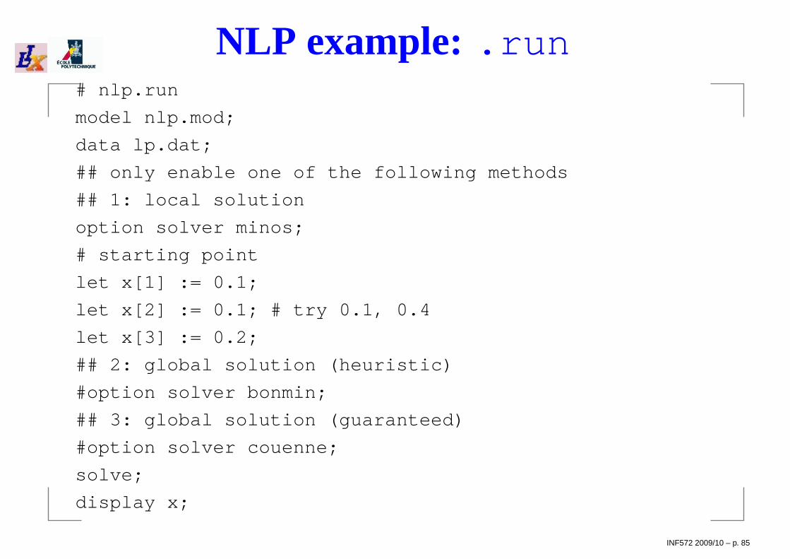
NLP example: .run# nlp.run

model nlp.mod;

data lp.dat;

## only enable one of the following methods

## 1: local solution

option solver minos;

# starting point

let x[1] := 0.1;

let x[2] := 0.1; # try 0.1, 0.4

let x[3] := 0.2;

## 2: global solution (heuristic)

#option solver bonmin;

## 3: global solution (guaranteed)

#option solver couenne;

solve;

display x;

INF572 2009/10 – p. 85

NLP example: output

MINOS 5.51: optimal solution found.140 iterations, objective -47.9955Nonlin evals: obj = 358, grad = 357, constrs = 358,x [ * ] :=1 0.12 0.13 4;

With x2 = 0.4 we get 47 iterations, objective −38.03000929and x = (2.84106, 1.37232, 0.205189).

INF572 2009/10 – p. 86

MINLP example: .mod# minlp.mod

param n integer, default 3;

param m integer, default 4;

set N := 1..n;

set M := 1..m;

param aM,N;

param bM;

param cN;

param epsilon := 0.1;

var xN >= 0, <= 4, integer;

minimize objective:

c[1] * x[1] * x[2] + c[2] * x[3]ˆ2 + c[3] * x[1] * x[2]/x[3] +

x[1] * x[3]ˆ3;

subject to constraintsi in M diff 4 :

sumj in N a[i,j] * x[j] <= b[i]/(x[i] + epsilon);

subject to constraint4 : prodj in N x[j] <= b[4];

INF572 2009/10 – p. 87

MINLP example: .run# minlp.run

model minlp.mod;

data lp.dat;

## only enable one of the following methods:

## 1: global solution (heuristic)

#option solver bonmin;

## 2: global solution (guaranteed)

option solver couenne;

solve;

display x;

INF572 2009/10 – p. 88

MINLP example: output

bonmin: Optimalx [ * ] :=1 02 43 4;

INF572 2009/10 – p. 89

Sudoku

INF572 2009/10 – p. 90

Sudoku: problem class

What is the problem class?

The class of all sudoku grids

Replace 1, . . . , 9 with a set K

Will need a set H = 1, 2, 3 to define 3× 3 sub-grids

An “instance” is a partial assignment of integers tocases in the sudoku grid

We model an empty sudoku grid, and then fix certainvariables at the appropriate values

INF572 2009/10 – p. 91

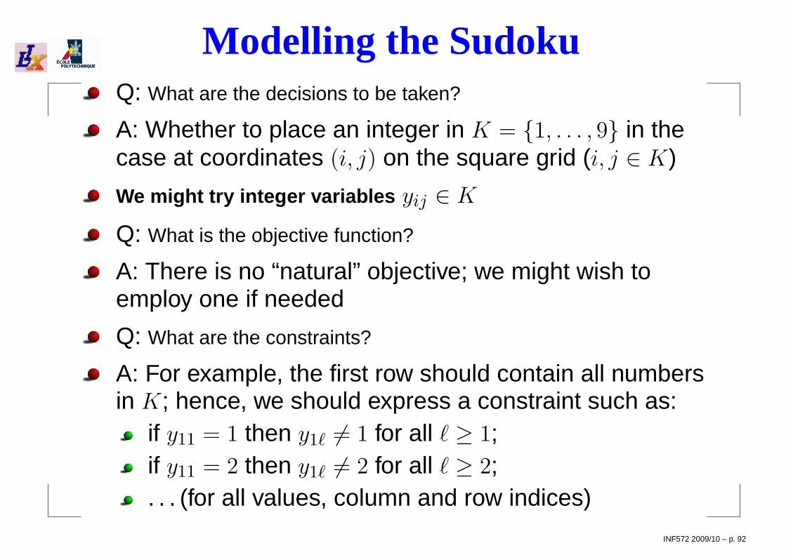
Modelling the SudokuQ: What are the decisions to be taken?

A: Whether to place an integer in K = 1, . . . , 9 in thecase at coordinates (i, j) on the square grid (i, j ∈ K)

We might try integer variables yij ∈ K

Q: What is the objective function?

A: There is no “natural” objective; we might wish toemploy one if needed

Q: What are the constraints?

A: For example, the first row should contain all numbersin K; hence, we should express a constraint such as:

if y11 = 1 then y1ℓ 6= 1 for all ℓ ≥ 1;if y11 = 2 then y1ℓ 6= 2 for all ℓ ≥ 2;. . . (for all values, column and row indices)

INF572 2009/10 – p. 92

Sudoku constraints 1In other words,

∀i, j, k ∈ K, ℓ 6= j (yij = k → yiℓ 6= k)

Put it another way: a constraint that says “all values shouldbe different”

In constraint programming (a discipline related to MP) thereis a constraint

∀i ∈ K AllDiff(yij | j ∈ K)

that asserts that all variables in its argument takedifferent values: we can attempt to implement it in MP

A set of distinct values has the pairwise distinctness property:∀i, p, q ∈ K yip 6= yiq, which can also be written as:

∀i, p < q ∈ K |yip − yiq| ≥ 1

INF572 2009/10 – p. 93

Sudoku constraints 2We also need the same constraints in each column:

∀j, p < q ∈ K |ypj − yqj | ≥ 1

. . . and in some appropriate 3× 3 sub-grids:1. let H = 1, . . . , 3 and α = |K|/|H|; for all h ∈ H

define Rh = i ∈ K | i > (h− 1)α ∧ i ≤ hα andCh = j ∈ K | j > (h− 1)α ∧ j ≤ hα

2. show that for all (h, l) ∈ H ×H, the set Rh × Cl

contains the case coordinates of the (h, l)-th 3× 3sudoku sub-grid

Thus, the following constraints must hold:

∀h, l ∈ H, i < p ∈ Rh, j < q ∈ Cl |yij − ypq| ≥ 1

INF572 2009/10 – p. 94

The Sudoku MINLP

The whole model is as follows:min 0

∀i, p < q ∈ K |yip − yiq| ≥ 1

∀j, p < q ∈ K |ypj − yqj | ≥ 1

∀h, l ∈ H, i < p ∈ Rh, j < q ∈ Cl |yij − ypq| ≥ 1

∀i ∈ K, j ∈ K yij ≥ 1

∀i ∈ K, j ∈ K yij ≤ 9

∀i ∈ K, j ∈ K yij ∈ Z

This is a nondifferentiable MINLP

MINLP solvers (BONMIN, MINLP_BB, COUENNE) can’tsolve it

INF572 2009/10 – p. 95

Absolute value reformulationThis MINLP, however, can be linearized:

|a− b| >= 1 ⇐⇒ a− b >= 1 ∨ b− a >= 1

For each i, j, p, q ∈ K we introduce a binary variablewpq

ij = 1 if yij − ypq ≥ 1 and 0 if ypq − yij ≥ 1

For all i, j, p, q ∈ K we add constraints1. yij − ypq ≥ 1−M(1− wpq

ij )

2. ypq − yij ≥ 1−Mwpqij

where M = |K|+ 1

This means: if wpqij = 1 then constraint 1 is active and 2

is always inactive (as ypq − yij is always greater than−|K|); if wpq

ij = 0 then 2 is active and 1 inactive

Transforms problematic absolute value terms intoadded binary variables and linear constraints

INF572 2009/10 – p. 96

The reformulated modelThe reformulated model is a MILP:

min 0

∀i, p < q ∈ K yip − yiq ≥ 1−M(1− wiqip)

∀i, p < q ∈ K yiq − yip ≥ 1−Mwiqip

∀j, p < q ∈ K ypj − yqj ≥ 1−M(1− wqjpj)

∀j, p < q ∈ K yqj − ypj ≥ 1−Mwqjpj

∀h, l ∈ H, i < p ∈ Rh, j < q ∈ Cl yij − ypq ≥ 1−M(1− wpqij )

∀h, l ∈ H, i < p ∈ Rh, j < q ∈ Cl ypq − yij ≥ 1−Mwpqij

∀i ∈ K, j ∈ K yij ≥ 1

∀i ∈ K, j ∈ K yij ≤ 9

∀i ∈ K, j ∈ K yij ∈ Z

It can be solved by CPLEX; however, it has O(|K|4) binary variableson a |K|2 cases grid with |K| values per case (O(|K|3) in total) —often an effect of bad modelling

INF572 2009/10 – p. 97

A better modelIn such cases, we have to go back to variable definitions

One other possibility is to define binary variables∀i, j, k ∈ K (xijk = 1) if the (i, j)-th case has value k, and 0otherwise

Each case must contain exactly one value

∀i, j ∈ K∑

k∈K

xijk = 1

For each row and value, there is precisely one columnthat contains that value, and likewise for cols

∀i, k ∈ K∑

j∈K

xijk = 1 ∧ ∀j, k ∈ K∑

i∈K

xijk = 1

Similarly for each Rh × Ch sub-square

∀h, l ∈ H, k ∈ K∑

i∈Rh,j∈Cl

xijk = 1

INF572 2009/10 – p. 98

The Sudoku MILPThe whole model is as follows:

min 0

∀i ∈ K, j ∈ K∑

k∈K

xijk = 1

∀i ∈ K, k ∈ K∑

j∈K

xijk = 1

∀j ∈ K, k ∈ K∑

i∈K

xijk = 1

∀h ∈ H, l ∈ H, k ∈ K∑

i∈Rh,j∈Cl

xijk = 1

∀i ∈ K, j ∈ K, k ∈ K xijk ∈ 0, 1

This is a MILP with O(|K|3) variables

Notice that there is a relation ∀i, j ∈ K yij =∑

k∈K

kxijk between the

MINLP and the MILP

The MILP variables have been derived by the MINLP ones by “disaggregation”

INF572 2009/10 – p. 99

Sudoku model fileparam Kcard integer, >= 1, default 9;

param Hcard integer, >= 1, default 3;

set K := 1..Kcard;

set H := 1..Hcard;

set RH;

set CH;

param alpha := card(K) / card(H);

param Instance K,K integer, >= 0, default 0;

let h in H R[h] := i in K : i > (h-1) * alpha and i <= h * alpha;

let h in H C[h] := j in K : j > (h-1) * alpha and j <= h * alpha;

var xK,K,K binary;

minimize nothing: 0;

subject to assignment i in K, j in K : sumk in K x[i,j,k] = 1;

subject to rows i in K, k in K : sumj in K x[i,j,k] = 1;

subject to columns j in K, k in K : sumi in K x[i,j,k] = 1;

subject to squares h in H, l in H, k in K :

sumi in R[h], j in C[l] x[i,j,k] = 1;

INF572 2009/10 – p. 100

Sudoku data file

param Instance :=

1 1 2 1 9 1 2 2 4 2 3 1 2 4 9

2 6 2 2 7 8 2 8 6 3 1 5 3 2 8

3 8 2 3 9 7 4 4 5 4 5 1 4 6 3

5 5 9 6 4 7 6 5 8 6 6 6 7 1 3

7 2 2 7 3 6 7 8 4 7 9 9 8 2 1

8 3 9 8 4 4 8 6 5 8 7 2 8 8 8

9 1 8 9 9 6 ;

INF572 2009/10 – p. 101

Sudoku run file

# sudoku

# replace "/dev/null" with "nul" if using Windows

option randseed 0;

option presolve 0;

option solver_msg 0;

model sudoku.mod;

data sudoku-feas.dat;

let i in K, j in K : Instance[i,j] > 0 x[i,j,Instance[i,j]] : = 1;

fix i in K, j in K : Instance[i,j] > 0 x[i,j,Instance[i,j]];

display Instance;

option solver cplex;

solve > /dev/null;

param Solution K, K;

if (solve_result = "infeasible") then

printf "instance is infeasible\n";

else

let i in K, j in K Solution[i,j] := sumk in K k * x[i,j,k];

display Solution;

INF572 2009/10 – p. 102

Sudoku AMPL output

liberti@nox$ cat sudoku.run | ampl

Instance [ * , * ]

: 1 2 3 4 5 6 7 8 9 :=

1 2 0 0 0 0 0 0 0 1

2 0 4 1 9 0 2 8 6 0

3 5 8 0 0 0 0 0 2 7

4 0 0 0 5 1 3 0 0 0

5 0 0 0 0 9 0 0 0 0

6 0 0 0 7 8 6 0 0 0

7 3 2 6 0 0 0 0 4 9

8 0 1 9 4 0 5 2 8 0

9 8 0 0 0 0 0 0 0 6

;

instance is infeasible

INF572 2009/10 – p. 103

Sudoku data file 2

But with a different data file. . .param Instance :=

1 1 2 1 9 1 2 2 4 2 3 1 2 4 9

2 6 2 2 7 8 2 8 6 3 1 5 3 2 8

3 8 2 3 9 7 4 4 5 4 5 1 4 6 3

5 5 9 6 4 7 6 5 8 6 6 6 7 1 3

7 2 2 7 8 4 7 9 9 8 2 1

8 3 9 8 4 4 8 6 5 8 7 2 8 8 8

9 1 8 9 9 6 ;

INF572 2009/10 – p. 104

Sudoku data file 2 grid

. . . corresponding to the grid below. . .

2 14 1 9 2 8 6

5 8 2 7

5 1 39

7 8 6

3 2 4 91 9 4 5 2 8

8 6

INF572 2009/10 – p. 105

Sudoku AMPL output 2

. . . we find a solution!liberti@nox$ cat sudoku.run | ampl

Solution [ * , * ]

: 1 2 3 4 5 6 7 8 9 :=

1 2 9 6 8 5 7 4 3 1

2 7 4 1 9 3 2 8 6 5

3 5 8 3 6 4 1 9 2 7

4 4 7 8 5 1 3 6 9 2

5 1 6 5 2 9 4 3 7 8

6 9 3 2 7 8 6 1 5 4

7 3 2 7 1 6 8 5 4 9

8 6 1 9 4 7 5 2 8 3

9 8 5 4 3 2 9 7 1 6

;

INF572 2009/10 – p. 106

Kissing Number Problem

INF572 2009/10 – p. 107

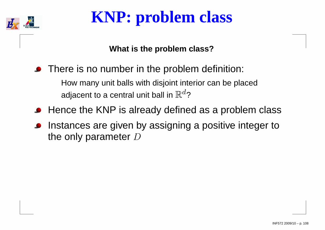
KNP: problem class

What is the problem class?

There is no number in the problem definition:How many unit balls with disjoint interior can be placed

adjacent to a central unit ball in Rd?

Hence the KNP is already defined as a problem class

Instances are given by assigning a positive integer tothe only parameter D

INF572 2009/10 – p. 108

Modelling the KNPQ: What are the decisions to be taken?

A: How many spheres to place, and where to place them

For each sphere, two types of variables

1. a logical one: yi = 1 if sphere i is present, and 0 otherwise

2. a D-vector of continuous ones: xi = (xi1, . . . , xiD), position ofi-th sphere center

Q: What is the objective function?

A: Maximize the number of spheres

Q: What are the constraints?

A: Two types of constraints

1. the i-th center must be at distance 2 from the central sphere if thei-th sphere is placed (center constraints)

2. for all distinct (and placed) spheres i, j, for their interior to bedisjoint their centers must be at distance ≥ 2 (distance constraints)

INF572 2009/10 – p. 109

Assumptions1. Logical variables y

Since the objective function counts the number of placedspheres, it must be something like

∑

i yi

What set N does the index i range over?

Denote k∗(d) the optimal solution to the KNP in Rd

Since k∗(d) is unknown a priori, we cannot know N a priori;however, without N , we cannot express the objective function

Assume we know an upper bound k to k∗(d); then we can defineN = 1, . . . , k (and D = 1, . . . , d)

2. Continuous variables x

Since any sphere placement is invariant by translation, we assume

that the central sphere is placed at the origin

Thus, each continuous variable xik (i ∈ N, k ∈ D) cannot attainvalues outside [−2, 2] (why?)

Limit continuous variables: −2 ≤ xik ≤ 2INF572 2009/10 – p. 110

Problem restatement

The above assumptions lead to a problem restatement

Given a positive integer k, what is the maximumnumber (smaller than k) of unit spheres with dis-joint interior that can be placed adjacent to a unit

sphere centered at the origin of Rd?

Each time assumptions are made for the sake of modelling, onemust always keep track of the corresponding changes to theproblem definition

The Objective function can now be written as:

max∑

i∈N

yi

INF572 2009/10 – p. 111

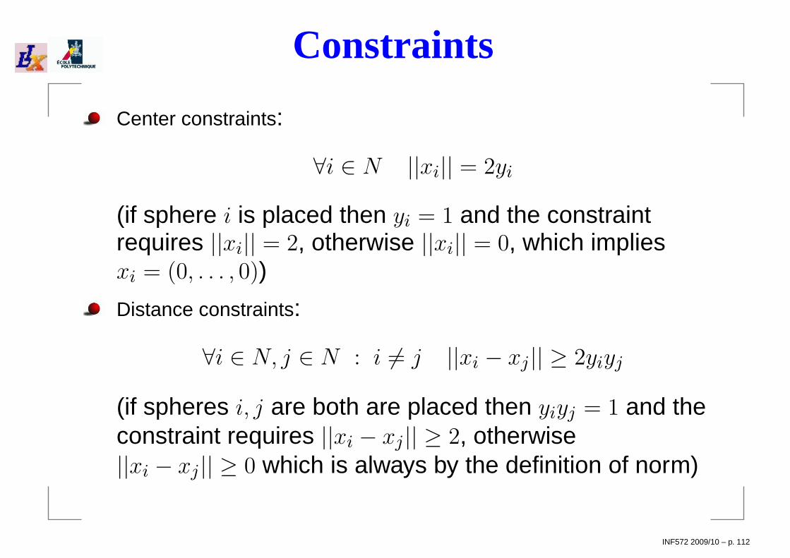
Constraints

Center constraints:

∀i ∈ N ||xi|| = 2yi

(if sphere i is placed then yi = 1 and the constraintrequires ||xi|| = 2, otherwise ||xi|| = 0, which impliesxi = (0, . . . , 0))

Distance constraints:

∀i ∈ N, j ∈ N : i 6= j ||xi − xj || ≥ 2yiyj

(if spheres i, j are both are placed then yiyj = 1 and theconstraint requires ||xi − xj || ≥ 2, otherwise||xi − xj || ≥ 0 which is always by the definition of norm)

INF572 2009/10 – p. 112

KNP model

max∑

i∈N

yi

∀i ∈ N√∑

k∈D

x2ik = 2yi

∀i ∈ N, j ∈ N : i 6= j√∑

k∈D

(xik − xjk)2 ≥ 2yiyj

∀i ∈ N yi ≥ 0

∀i ∈ N yi ≤ 1

∀i ∈ N, k ∈ D xik ≥ −2

∀i ∈ N, k ∈ D xik ≤ 2

∀i ∈ N yi ∈ Z

For brevity, we shall write yi ∈ 0, 1 and xik ∈ [−2, 2]

INF572 2009/10 – p. 113

Reformulation 1

Solution times for NLP/MINLP solvers often alsodepends on the number of nonlinear terms

We square both sides of the nonlinear constraints, andnotice that since yi are binary variables, y2

i = yi for alli ∈ N ; we get:

∀i ∈ N∑

k∈D

x2ik = 4yi

∀i 6= j ∈ N∑

k∈D

(xik − xjk)2 ≥ 4yiyj

which has fewer nonlinear terms than the originalproblem

INF572 2009/10 – p. 114

Reformulation 2Distance constraints are called reverse convex (because ifwe replace ≥ with ≤ the constraints become convex);these constraints often cause solution times to lengthenconsiderably

Notice that distance constraints are repeated when i, jare swapped

Change the quantifier to i ∈ N, j ∈ N : i < j reduces thenumber of reverse convex constraints in the problem;get:

∀i ∈ N∑

k∈D

x2ik = 4yi

∀i < j ∈ N∑

k∈D

(xik − xjk)2 ≥ 4yiyj

INF572 2009/10 – p. 115

KNP model revisited

max∑

i∈N

yi

∀i ∈ N∑

k∈D

x2ik = 4yi

∀i ∈ N, j ∈ N : i < j∑

k∈D

(xik − xjk)2 ≥ 4yiyj

∀i ∈ N, k ∈ D xik ∈ [−2, 2]

∀i ∈ N yi ∈ 0, 1

This formulation is a (nonconvex) MINLP

INF572 2009/10 – p. 116

KNP model file

# knp.mod

param d default 2;

param kbar default 7;

set D := 1..d;

set N := 1..kbar;

var yi in N binary;

var xi in N, k in D >= -2, <= 2;

maximize kstar : sumi in N y[i];

subject to centeri in N : sumk in D x[i,k]ˆ2 = 4 * y[i];

subject to distancei in N, j in N : i < j :

sumk in D (x[i,k] - x[j,k])ˆ2 >= 4 * y[i] * y[j];

INF572 2009/10 – p. 117

KNP data file

Since the only data are the parameters d and k (twoscalars), for simplicity we do not use a data file at all, andassign values in the model file instead

INF572 2009/10 – p. 118

KNP run file

# knp.runmodel knp.mod;option solver boncouenne;solve;display x,y;display kstar;

INF572 2009/10 – p. 119

KNP solution (?)

We tackle the easiest possible KNP instance (d = 2),and give it an upper bound k = 7

It is easy to see that k∗(2) = 6 (place 6 circles adjacentto another circle in an exagonal lattice)

Yet, after several minutes of CPU time COUENNE has notmade any progress from the trivial feasible solutiony = 0, x = 0

Likewise, heuristic solvers such as BONMIN andMINLP BB only find the trivial zero solution and exit

INF572 2009/10 – p. 120

What do we do next?

In order to solve the KNP and deal with other difficultMINLPs, we need more advanced techniques

INF572 2009/10 – p. 121

Some useful MP theory

INF572 2009/10 – p. 122

Open sets

In general, MP cannot directly model problems involvingsets which are not closed in the usual topology (such ase.g. open intervals)

The reason is that the minimum/maximum of anon-closed set might not exist

E.g. what is minx∈(0,1)

x? Since (0, 1) has no minimum (for

each δ ∈ (0, 1), δ2 < δ and is in (0, 1)), the question has

no answer

This is why the MP language does not allow writing constraints thatinvolve the <, > and 6= relations

Sometimes, problems involving open sets can bereformulated exactly to problems involving closed sets

INF572 2009/10 – p. 123

Best fit hyperplane 1Consider the following problem:

Given m points p1, . . . , pm ∈ Rn, find the hyperplanew1x1 + · · ·+ wnxn = w0 minimizing the piecewise linear formf(p, w) =

∑

i∈P

| ∑j∈N

wjpij − w0|

Mathematical programming formulation:

1. Sets : P = 1, . . . , m, N = 1, . . . , n2. Parameters: ∀i ∈ P pi ∈ Rn

3. Decision variables : ∀j ∈ N wj ∈ R, w0 ∈ R

4. Objective : minw f(p, w)

5. Constraints : none

Trouble: w = 0 is the obvious, trivial solution of no interest

We need to enforce a constraint (w1, . . . , wn, w0) 6= (0, . . . , 0)

Bad news: Rn+1 r (0, . . . , 0) is not a closed set

INF572 2009/10 – p. 124

Best fit hyperplane 2We can implicitly impose such a constraint by transforming theobjective function to minw

f(p,w)||w|| (for some norm || · ||)

This implies that w is nonzero but the feasible region is Rn+1, whichis both open and closed

Obtain fractional objective — difficult to solve

Suppose w∗ = (w∗, w∗

0) ∈ Rn+1 is an optimal solution to the aboveproblem

Then for all d > 0, f(dw∗, p) = df(w∗, p)

Hence, it suffices to determine the optimal direction of w∗, because theactual vector length simply scales the objective function value

Can impose constraint ||w|| = 1 and recover original objective

Solve reformulated problem:

minf(w, p) | ||w|| = 1

INF572 2009/10 – p. 125

Best fit hyperplane 3The constraint ||w|| = 1 is a constraint schema: we mustspecify the norm

Some norms can be reformulated to linear constraints,some cannot

max-norm (l∞) 2-sphere (square), Euclidean norm (l2)2-sphere (circle), abs-norm (l1) 2-sphere (rhombus)

max- and abs-norms are piecewise linear, they can belinearized exactly by using binary variables (see later)

INF572 2009/10 – p. 126

Convexity in practiceRecognizing whether an arbitrary function is convex isan undecidable problem

For some functions, however, this is possibleCertain functions are known to be convex (such as allaffine functions, cx2n for n ∈ N and c ≥ 0, exp(x),− log(x))Norms are convex functionsThe sum of two convex functions is convex

Application of the above rules repeatedly sometimesworks (for more information, see Disciplined ConvexProgramming [Grant et al. 2006])

Warning: problems involving integer variables are in general notconvex; however, if the objective function and constraints are convex

forms, we talk of convex MINLPs

INF572 2009/10 – p. 127

Recognizing convexity 1

Consider the following mathematical program

minx,y∈[0,10]

8x2 − 17xy + 10y2

x− y ≥ 1

xy ≤ 1

x

Objective function and constraints contain nonconvexterm xy

Constraint 2 is ≤ 1x ; the function 1

x is convex (in thepositive orthant) but constraint sense makes itnonconvex

Is this problem convex or not?

INF572 2009/10 – p. 128

Recognizing convexity 2The objective function can be written as (x, y)TQ(x, y)

where Q =

(

8 −8

−9 10

)

The eigenvalues of Q are 9±√

73 (both positive), hencethe Hessian of the objective is positive definite, hencethe objective function is convex

The affine constraint x− y ≥ 1 is convex by definition

xy ≤ 1x can be reformulated as follows:

1. Take logarithms of both sides: log xy ≤ log 1x

2. Implies log x + log y ≥ − log x⇒ −2 log x− log y ≤ 0

3. − log is a convex function, sum of convex functions isconvex, convex ≤ affine is a convex constraint

Thus, the constraint is convexINF572 2009/10 – p. 129

Recognizing convexity 3model; param eps=1e-6;

var x <= 10, >= -10;

var y <= 10, >= -10;

minimize f: 8 * xˆ2 -17 * x* y + 10 * yˆ2;

subject to c1: x-y >= 1;

subject to c2: x * y <= 1/(x+eps);

option solver_msg 0;

printf "solving with sBB (couenne)\n";

option solver couenne;

solve > /dev/null;

display x,y;

printf "solving with local NLP solver (ipopt)\n";

option solver ipopt; let x := 0; let y := 0;

solve > /dev/null; display x,y;

Get approx. same solution (1.46, 0.46) from COUENNE and IPOPT

INF572 2009/10 – p. 130

Total Unimodularity

A matrix A is Totally Unimodular (TUM) if all invertiblesquare submatrices of A have determinant ±1Thm.If A is TUM, then all vertices of the polyhedron

x ≥ 0 | Ax ≤ b

have integral components

Consequence: if the constraint matrix of a given MILP isTUM, then it suffices to solve the relaxed LP to get asolution for the original MILP

An LP solver suffices to solve the MILP to optimality

INF572 2009/10 – p. 131

TUM in practice 1

If A is TUM, AT and (A|I) are TUM

TUM Sufficient conditions. An m× n matrix A is TUM if:1. for all i ≤ m, j ≤ n we have aij ∈ 0, 1,−1;2. each column of A contains at most 2 nonzero

coefficients;3. there is a partition R1, R2 of the set of rows such that

for each column j,∑

i∈R1aij −

∑

i∈R2aij = 0.

Example: take R1 = 1, 3, 4, R2 = 2

1 0 1 1 0 0

0 −1 0 1 −1 1

−1 −1 0 0 0 1

0 0 −1 0 −1 0

INF572 2009/10 – p. 132

TUM in practice 2

Consider digraph G = (V,A) with nonnegative variablesxij ∈ R+ defined on each arc

Flow constraints ∀i ∈ V∑

(i,j)∈A

xij −∑

(j,i)∈A

xji = bi yield a

TUM matrix (partition: R1 = all rows, R2 = ∅— prove it)

Maximum flow problems can be solved to integrality bysimply solving the continuous relaxation with an LPsolver

The constraints of the set covering problem do not form a TUM. Toprove this, you just need to find a counterexample

INF572 2009/10 – p. 133

Maximum flow problem

Given a network on a directed graph G = (V,A) with asource node s, a destination node t, and integer capacitiesuij on each arc (i, j). We have to determine the maximumintegral amount of material flow that can circulate on thenetwork from s to t. The variables xij ∈ Z, defined for eacharc (i, j) in the graph, denote the number of flow units.

maxx

∑

(s,i)∈A

xsi

∀ i ≤ V,i 6= s

i 6= t

∑

(i,j)∈A

xij =∑

(j,i)∈A

xji

∀(i, j) ∈ A 0 ≤ xij ≤ uij

∀(i, j) ∈ A xij ∈ Z

31

4

i

xji

xij

INF572 2009/10 – p. 134

Max Flow Example 1

1 2 3

4 5 6 7

4

5

21

7

6

5

1

13

2

7

arc capacities as shown in italics: find the maximum flowbetween node s = 1 and t = 7

INF572 2009/10 – p. 135

Max Flow: MILP formulation

Sets : V = 1, . . . , n, A ⊆ V × V

Parameters : s, t ∈ V , u : A→ R+

Variables : x : A→ Z+

Objective : max∑

(s,i)∈A

xsi

Constraints : ∀i ∈ V r s, t ∑

(i,j)∈A

xij =∑

(j,i)∈A

xji

INF572 2009/10 – p. 136

Max Flow: .mod file# maxflow.modparam n integer, > 0, default 7;param s integer, > 0, default 1;param t integer, > 0, default n;set V := 1..n;set A within V,V;param uA >= 0;

var x(i,j) in A >= 0, <= u[i,j], integer;

maximize flow : sum(s,i) in A x[s,i];

subject to flowconsi in V diff s,t :sum(i,j) in A x[i,j] = sum(j,i) in A x[j,i];

INF572 2009/10 – p. 137

Max Flow: .dat file

# maxflow.datparam : A : u :=

1 2 51 4 41 5 12 4 23 2 13 4 13 7 24 5 75 3 65 6 56 2 36 7 7 ;

INF572 2009/10 – p. 138

Max Flow: .run file

# maxflow.runmodel maxflow.mod;data maxflow.dat;option solver_msg 0;option solver cplex;solve;for (i,j) in A : x[i,j] > 0

printf "x[%d,%d] = %g\n", i,j,x[i,j];display flow;

INF572 2009/10 – p. 139

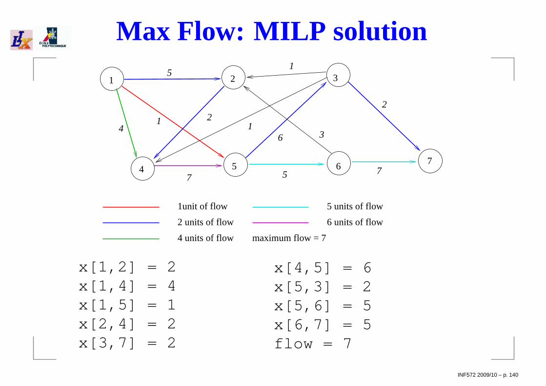
Max Flow: MILP solution

5 units of flow

6 units of flow

1 2 3

4 5 6 7

4

5

21

7

6

5

1

13

2

7

1unit of flow

2 units of flow

4 units of flow maximum flow = 7

x[1,2] = 2x[1,4] = 4x[1,5] = 1x[2,4] = 2x[3,7] = 2

x[4,5] = 6x[5,3] = 2x[5,6] = 5x[6,7] = 5flow = 7

INF572 2009/10 – p. 140

Max Flow: LP solution

Relax integrality constraints (take away integer keyword)

5 units of flow

6 units of flow

1 2 3

4 5 6 7

4

5

21

7

6

5

1

13

2

7

1unit of flow

2 units of flow

4 units of flow maximum flow = 7

Get the same solution

INF572 2009/10 – p. 141

Reformulations

INF572 2009/10 – p. 142

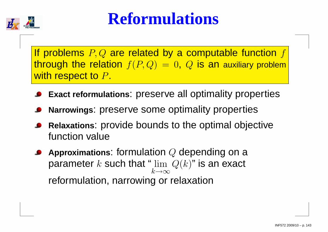
Reformulations

If problems P,Q are related by a computable function fthrough the relation f(P,Q) = 0, Q is an auxiliary problemwith respect to P .

Exact reformulations : preserve all optimality properties

Narrowings : preserve some optimality properties

Relaxations : provide bounds to the optimal objectivefunction value

Approximations : formulation Q depending on aparameter k such that “ lim

k→∞Q(k)” is an exact

reformulation, narrowing or relaxation

INF572 2009/10 – p. 143

Exact reformulationsP

Q

F

F LL

GG

φ

φ|L

φ|G

Main idea: if we find an optimum of Q, we can map it back to the sametype of optimum of P , and for all optima of P , there is a correspond-ing optimum in Q. Also known as exact reformulation

INF572 2009/10 – p. 144

NarrowingsP

Q

F

F

G

G

φ

φ|G

Main idea: if we find a global optimum of Q, we can mapit back to a global optimum of P . There may be optimaof P without a corresponding optimum in Q.

INF572 2009/10 – p. 145

Relaxations

A problem Q is a relaxation of P if the globally optimalvalue of the objective function min fQ of Q is a lowerbound to that of P .

INF572 2009/10 – p. 146

ApproximationsQ is an approximation of P if there exist: (a) an auxiliary problemQ∗ of P ; (b) a sequence Qk of problems; (c) an integer ℓ > 0;such that:

1. Q = Qℓ

2. ∀ objective f∗ in Q∗ there is a sequence of objectives fk of Qk

converging uniformly to f∗;

3. ∀ constraint l∗i ≤ g∗i (x) ≤ u∗i of Q∗ there is a sequence of constraints

lki ≤ gki (x) ≤ uk

i of Qk such that gki converges uniformly to g∗i , lki

converges to l∗i and uki to u∗

i

There can be approximations to exact reformulations, narrowings,relaxations.

Q1, Q2, Q3, Qℓ, Q∗ P. . .. . .

approximation of P

〈auxiliary problem of〉

INF572 2009/10 – p. 147

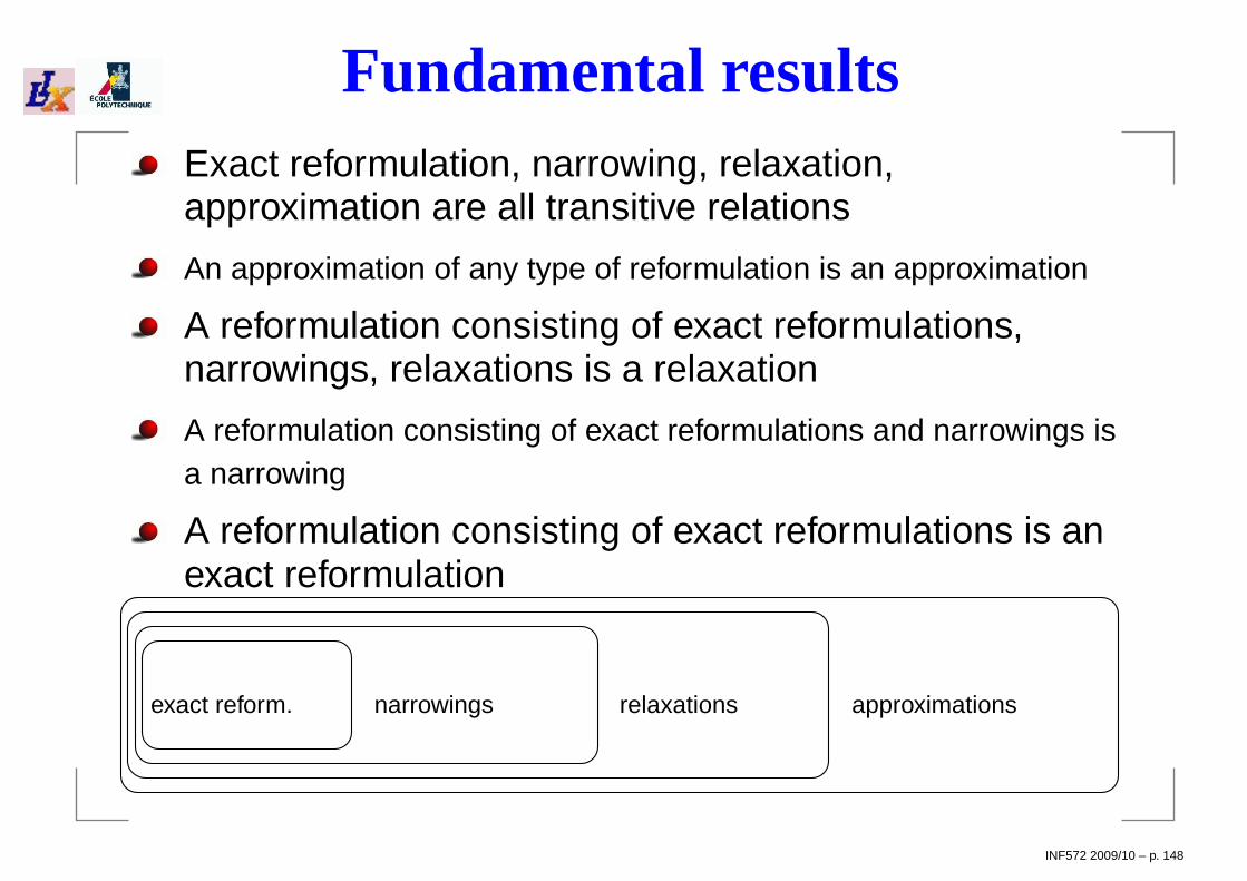
Fundamental resultsExact reformulation, narrowing, relaxation,approximation are all transitive relations

An approximation of any type of reformulation is an approximation

A reformulation consisting of exact reformulations,narrowings, relaxations is a relaxation

A reformulation consisting of exact reformulations and narrowings isa narrowing

A reformulation consisting of exact reformulations is anexact reformulation

exact reform. narrowings relaxations approximations

INF572 2009/10 – p. 148

Reformulations in practice

Reformulations are used to transform problems intoequivalent (or related) formulations which are somehow“better”

Basic reformulation operations :

1. change parameter values2. add / remove variables3. adjoin / remove constraints4. replace a term with another term (e.g. a product xy

with a new variable w)

INF572 2009/10 – p. 149

Product of binary variablesConsider binary variables x, y and a cost c to be addedto the objective function only of xy = 1

⇒ Add term cxy to objective

Problem becomes mixed-integer (some variables arebinary) and nonlinear

Reformulate “xy” to MILP form (PRODBIN reform.):

replace xy by z

add z ≤ y , z ≤ x

z ≥ 0, z ≥ x + y − 1

x, y ∈ 0, 1 ⇒z = xy

INF572 2009/10 – p. 150

Application to the KNPIn the RHS of the KNP’s distance constraints we have 4yiyj , whereyi, yj are binary variables

We apply PRODBIN (call the added variable wij):

minP

i∈N

yi

∀i ∈ NP

k∈D

x2ik

= 4yi

∀i ∈ N, j ∈ N : i < jP

k∈D

(xik − xjk)2 ≥ 4wij

∀i ∈ N, j ∈ N : i < j wij ≤ yi

∀i ∈ N, j ∈ N : i < j wij ≤ yj

∀i ∈ N, j ∈ N : i < j wij ≥ yi + yj − 1

∀i ∈ N, j ∈ N : i < j wij ∈ [0, 1]

∀i ∈ N, k ∈ D xik ∈ [−2, 2]

∀i ∈ N yi ∈ 0, 1

9

>

>

>

>

>

>

>

>

>

>

>

>

>

>

>

>

>

>

>

>

>

>

=

>

>

>

>

>

>

>

>

>

>

>

>

>

>

>

>

>

>

>

>

>

>

;

Still a MINLP, but fewer nonlinear terms

Still numerically difficult (2h CPU time to find k∗(2) ≥ 5)INF572 2009/10 – p. 151

Product of bin. and cont. vars.PRODBINCONT reformulation

Consider a binary variable x and a continuous variabley ∈ [yL, yU ], and assume product xy is in the problem

Replace xy by an added variable w

Add constraints:

w ≤ yUx

w ≥ yLx

w ≤ y + yL(1− x)

w ≥ y − yU (1− x)

Exercise 1 : show that PRODBINCONT is an exact reformulation

Exercise 2 : show that if y ∈ 0, 1 then PRODBINCONT is equivalent toPRODBIN

INF572 2009/10 – p. 152

Prod. cont. vars.: approximationBILINAPPROX approximation

Consider x ∈ [xL, xU ], y ∈ [yL, yU ] and product xy

Suppose xU − xL ≤ yU − yL, consider an integer d > 0

Replace [xL, xU ] by a finite set

D = xL + (i− 1)γ | 1 ≤ i ≤ d, where γ = xU−xL

d−1

→

INF572 2009/10 – p. 153

BILINAPPROX

Replace the product xy by a variable w

Add binary variables zi for i ≤ d

Add assignment constraint for zi’s

∑

i≤d

zi = 1

Add definition constraint for x:

x =∑

i≤d

(xL + (i− 1)γ)zi

(x takes exactly one value in D)

Add definition constraint for w

w =∑

i≤d

(xL + (i− 1)γ)ziy (7)

Reformulate the products ziy via PRODBINCONT

INF572 2009/10 – p. 154

BILINAPPROX2

BILINAPPROX2 : problem P has a term xy where x ∈[xL, xU ], y ∈ [yL, yU ] are continuous; assume xU −xL ≤ yU − yL

1. choose integer k > 0; add q = qi | 0 ≤ i ≤ kto P so that q0 = xL, qk = xU , qi < qi+1 for all i

2. add continuous variable w ∈ [wL, wU ] (com-puted from ranges of x, y by interval arithmetic)and replace term xy by w

3. add binary variables zi for 1 ≤ i ≤ k and con-straint

∑

i≤k zi = 1

4. for all 1 ≤ i ≤ k add constraints:

k → ∞: get iden-tity (exact) reformu-lation

k∑

j=1

qj−1zj ≤ xi ≤k∑

j=1

qjzj

qi+qi−1

2 y − (wU − wL)(1− zi) ≤ w ≤ qi+qi−1

2 y + (wU − wL)(1− zi),

INF572 2009/10 – p. 155

Relaxing bilinear termsRRLTRELAX : quadratic problem P with terms xixj (i < j) and constrs

Ax = b (x can be bin, int, cont); perform exact reformulation RRLT

first:

1. add continuous variables wij (let wi = (wi1, . . . , w1n))

2. replace product xixj with wij (for all i, j)

3. add the reduced RLT (RRLT) system ∀k Awk − bxk = 0

4. find a partition (B, N) of basic/nonbasic variables of ∀k Awk = 0

such that B corresponds to variables with smallest range

5. for all (i, j) ∈ N add constraints wij = xixj (†)then replace nonlinear constraints (†) with McCormick’s envelopes

wij ≥ maxxLi xj + xL

j xi − xLi xL

j , xUi xj + xU

j xi − xUi xU

j

wij ≤ minxUi xj + xL

j xi − xUi xL

j , xLi xj + xU

j xi − xLi xU

j A

BC

D

−1−0.5

0 0.5

1 −1−0.5

0 0.5

1−1

−0.5

0

0.5

1

The effect of RRLT is that of using information in Ax = b to eliminatesome of the problematic product terms (those with indices in B) INF572 2009/10 – p. 156

Linearizing the l∞ norm

INFNORM [Coniglio et al., MSc Thesis, 2007]. P hasvars x ∈ [−1, 1]d and constr. ||x||∞ = 1,s.t. x∗ ∈ F(P )↔ −x∗ ∈ F(P ) and f(x∗) = f(−x∗).1. ∀k ≤ d add binary var uk

2. delete constraint ||x||∞ = 1

3. add constraints:

∀k ≤ d xk ≥ 2uk − 1∑

k≤d

uk = 1.

Narrowing INFNORM(P ) cuts away all optima havingmaxk |xk| = 1 with xk < 1 for all k ≤ d

INF572 2009/10 – p. 157

Approximating squaresINNERAPPROXSQ : P has a continuous variable

x ∈ [xL, xU ] and a term x2 appearing as aconvex term in an objective or constraint

1. add parameters n ∈ N, ε = xU−xL

n−1 ,xi = xL + (i− 1)ε for i ≤ n

2. add a continuous variable w ∈ [wL, wU ],where wL = 0 if xLxU ≤ 0 ormin((xL)2, (xU )2) otherwise andwU = max((xL)2, (xU )2)

3. replace all occurrences of term x2 with w

4. add constraints∀i ≤ n w ≥ (xi + xi−1)x− xixi−1.

Replace convex term by piecewise linear ap-proximation

x

s

n → ∞: getidentity (exact)reformulation

INF572 2009/10 – p. 158

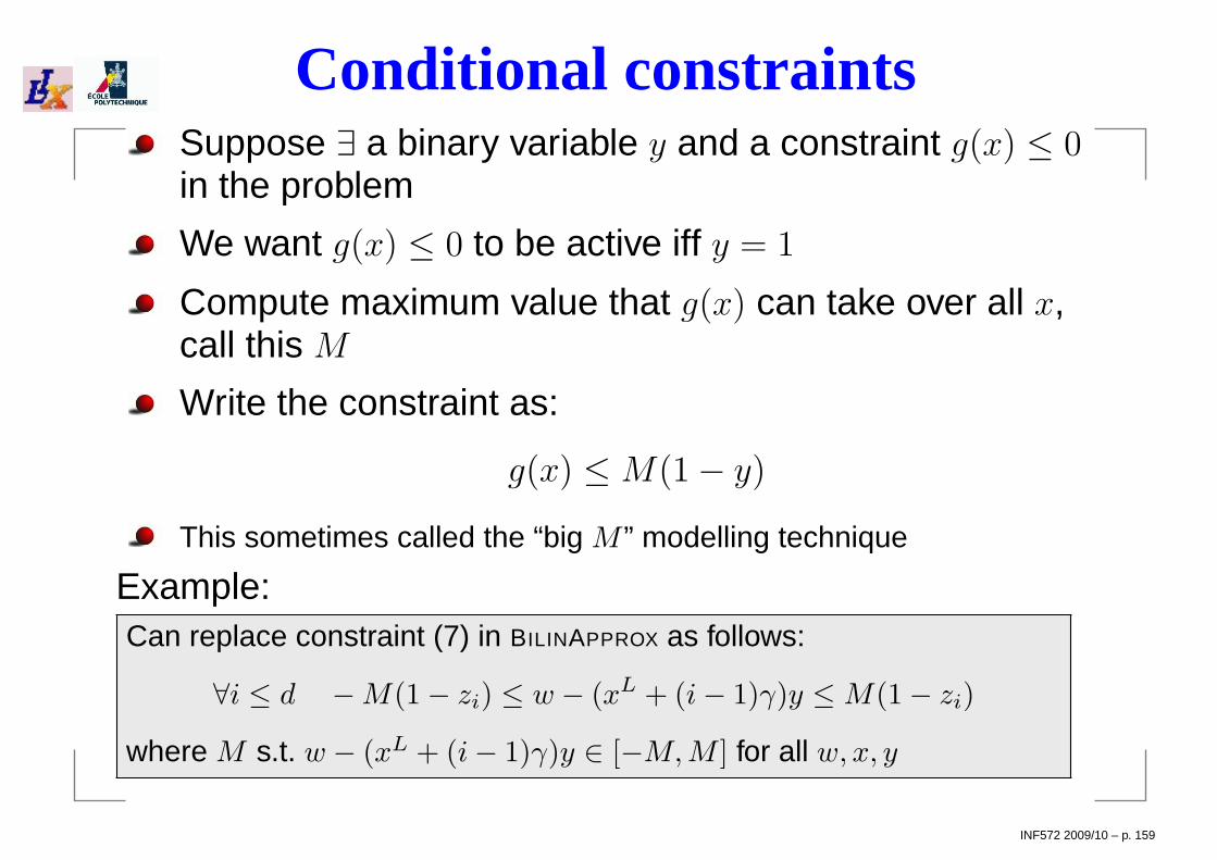
Conditional constraintsSuppose ∃ a binary variable y and a constraint g(x) ≤ 0in the problem

We want g(x) ≤ 0 to be active iff y = 1

Compute maximum value that g(x) can take over all x,call this M

Write the constraint as:

g(x) ≤M(1− y)

This sometimes called the “big M ” modelling technique

Example:Can replace constraint (7) in BILINAPPROX as follows:

∀i ≤ d −M(1− zi) ≤ w − (xL + (i− 1)γ)y ≤M(1− zi)

where M s.t. w − (xL + (i− 1)γ)y ∈ [−M, M ] for all w, x, y

INF572 2009/10 – p. 159

Symmetry

INF572 2009/10 – p. 160

ExampleConsider the problem

min x1 + x2

3x1 + 2x2 ≥ 1

2x1 + 3x2 ≥ 1

x1, x2 ∈ 0, 1

AMPL code:set J := 1..2;

var xJ binary;

minimize f: sumj in J x[j];

subject to c1: 3 * x[1] + 2 * x[2] >= 1;

subject to c2: 2 * x[1] + 3 * x[2] >= 1;

option solver cplex;

solve;

display x;

The solution (given byCPLEX) is x1 = 1, x2 = 0

If you swap x1 with x2, you

obtain the same problem, with

swapped constraints

Hence, x1 = 0, x2 = 1 isalso an optimal solution!

INF572 2009/10 – p. 161

Permutations

We can represent permutations by maps N→ N

The permutation of our example is0

@

1 2↓ ↓2 1

1

A

Permutations are usually written as cycles: e.g. for a

permutation0

@

1 2 3↓ ↓ ↓3 1 2

1

A, which sends 1→ 3, 3→ 2 and

2→ 1, we write (1, 3, 2) to mean 1→ 3→ 2(→ 1)

The permutation of our example is (1, 2) — a cycle oflength 2 (also called a transposition, or swap)

INF572 2009/10 – p. 162

CyclesCycles can be multiplied together, but the multiplicationis not commutative: (1, 2, 3)(1, 2) = (1, 3) and(1, 2)(1, 2, 3) = (2, 3)

The identity permutation e fixes all N

Notice (1, 2)(1, 2) = e and (1, 2, 3)(1, 3, 2) = e, so(1, 2) = (1, 2)−1 and (1, 3, 2) = (1, 2, 3)−1

Cycles are disjoint when they have no common element

Thm. Disjoint cycles commute

Thm. Every permutation can be written uniquely (up toorder) as a product of disjoint cycles

For each permutation π, let Γ(π) be the set of its disjointcycles

INF572 2009/10 – p. 163

GroupsA group is a set G together with a multiplicationoperation, an inverse operation, and an identity elemente ∈ G, such that:1. ∀g, h ∈ G (gh ∈ G) (multiplication closure)

2. ∀g ∈ G (g−1 ∈ G) (inverse closure)3. ∀f, g, h ∈ G ((fg)h = f(gh)) (associativity)4. ∀g ∈ G (eg = g) (identity )

5. ∀g ∈ G (g−1g = e) (inverse)

The set e is a group (denoted by 1) called the trivialgroup

The set of all permutations over 1, . . . , n is a group,called the symmetric group of order n, and denoted by Sn

For all B ⊆ 1, . . . , n define SB as the symmetric groupover the symbols of B

INF572 2009/10 – p. 164

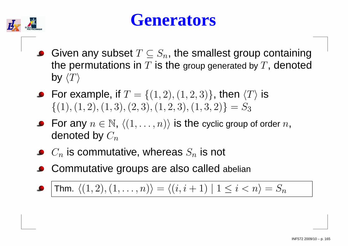
Generators

Given any subset T ⊆ Sn, the smallest group containingthe permutations in T is the group generated by T , denotedby 〈T 〉For example, if T = (1, 2), (1, 2, 3), then 〈T 〉 is(1), (1, 2), (1, 3), (2, 3), (1, 2, 3), (1, 3, 2) = S3

For any n ∈ N, 〈(1, . . . , n)〉 is the cyclic group of order n,denoted by Cn

Cn is commutative, whereas Sn is not

Commutative groups are also called abelian

Thm. 〈(1, 2), (1, . . . , n)〉 = 〈(i, i + 1) | 1 ≤ i < n〉 = Sn

INF572 2009/10 – p. 165

Subgroups and homomorphisms

A subgroup of a group G is a subset H of G which is also a group(denoted by H ≤ G); e.g. C3 = e, (1, 2, 3), (1, 3, 2) is a subgroup ofS3

Given two groups G, H, a map φ : G→ H such that∀f, g ∈ G ( φ(fg) = φ(f)φ(g) ) is a homomorphism

Kerφ = g ∈ G | φ(g) = e is the kernel of φ (Kerφ ≤ G)

Imφ = h ∈ H | ∃g ∈ G (h = φ(g)) is the image of φ (Imφ ≤ H)

If φ is injective and surjective (i.e. if Kerφ = 1 and Imφ = H), then φ isan isomorphism, denoted by G ∼= H

Thm.[Lagrange] For all groups G and H ≤ G, |H| divides |G|

Thm.[Cayley] Every finite group is isomorphic to a subgroup of Sn forsome n ∈ N

INF572 2009/10 – p. 166

Normal subgroups

Let H ≤ G; for all g ∈ G, gH = gh | h ∈ H andHg = hg | h ∈ H are in general subsets (notnecessarily subgroups) of G, and in general gH 6= Hg

If ∀g ∈ G (gH = Hg) then H is a normal subgroup of G,denoted by H ⊳ G (e.g. C3 ⊳ S3)

If H ⊳ G, then gH | g ∈ G is denoted by G/H and hasa group structure with multiplication (fH)(gH) = (fg)H,inverse (gH)−1 = (g−1)H and identity eH = H

For every group homomorphism φ, Kerφ ⊳ G andG/Kerφ ∼= Imφ

INF572 2009/10 – p. 167

Group actions

Given a group G and a set X, the action of G on X is aset of mappings αg : X → X for all g ∈ G, such thatαg(x) = (gx) ∈ X for all x ∈ X

Essentially, the action of G on X is the definition of whathappens to x ∈ X when g is applied to it

For example, if X = Rn and G = Sn, a possible action ofG on X is given by gx being the vector x withcomponents permuted according to g (e.g. ifx = (0.1,−2,

√2) and g = (1, 2), then gx = (−2, 0.1,

√2))

Convention: left multiplication if x is a column vector(αg(x) = gx), right if x is a row vector (αg(x) = xg): treatg as a matrix

INF572 2009/10 – p. 168

OrbitsIf G acts on X ⊆ Rn, for all x ∈ X, Gx = gx | g ∈ Gis the orbit of x w.r.t. G

1

2

1 2

2

1

x = (2, 1, 0)

gx=(1,2,0)g=(1,2)

gx=(0,2,1)g=(1,2,3)

gx=(0,1,2)g=(1,3)

gx=(1,0,2)g=(1,3,2)

gx=(2,0,1)g=(2,3)

S3(2, 1, 0)T

INF572 2009/10 – p. 169

Stabilizers

Given Y ⊆ X, the point-wise stabilizer of Y w.r.t. G is asubgroup H ≤ G such that hy = y for all h ∈ H, y ∈ Y

pointwise

y1y1 y2y2

y3y3

y4y4

h

Y

X

setwise

y1y1 y2y2

y3y3

y4y4

h

Y

X

The set-wise stabilizer of Y w.r.t. G is a subgroup H ≤ Gsuch that HY = Y (denote H by stab(Y,G))

Let π ∈ Sn with disjoint cycle product σ1 · · ·σk andN ⊆ 1 . . . , nπ[N ] =

∏

j≤k

σj∈stab(N,Sn)

σj: restriction of π to N

INF572 2009/10 – p. 170

Groups and graphsGiven a digraph G = (V,A) with V = v1, . . . , vn, theaction of π ∈ Sn on G is the natural action of π on V

π is a graph automorphism if ∀(i, j) ∈ A (π(i), π(j)) ∈ A

For example:

G1

1 2

34G2

3 2

14G3

4 1

23

G2 = (1, 3)G1 is a graph automorphism of G1

G3 = (1, 2, 3, 4)G1 is not an automorphism of G1: e.g. (4, 2) ∈ A but(π(4), π(2)) = (1, 3) 6∈ A

The automorphism group of G1 is 〈e, (1, 3)〉 ∼= C2 (denotedby Aut(G1))

INF572 2009/10 – p. 171

Back to MP: Symmetries and BB

Symmetries are bad for Branch-and-Bound techniques:many branches will contain (symmetric) optimalsolutions and therefore will not be pruned by bounding⇒ deep and large BB trees

-Inf

1.5 2

2 2

← BB tree for symmetricproblem

BB tree for “problemmodulo symmetries”→

-Inf

2 2

How do we write a “mathematical programming formu-lation modulo symmetries”?

INF572 2009/10 – p. 172

Solution symmetriesThe set of solutions of the following problem:

min x11 +x12 +x13 +x21 +x22 +x23

x11 +x12 +x13 ≥ 1

x21 +x22 +x23 ≥ 1

x11 +x21 ≥ 1

x12 +x22 ≥ 1

x13 +x23 ≥ 1

is G(P ) =(0, 1, 1, 1, 0, 0), (1, 0, 0, 0, 1, 1), (0, 0, 1, 1, 1, 0),

(1, 1, 0, 0, 0, 1), (1, 0, 1, 0, 1, 0), (0, 1, 0, 1, 0, 1)

G∗ = stab(G(P ), Sn) is the solution group (variable permutations keeping

G(P ) fixed)

For the above problem, G∗ is〈(2, 3)(5, 6), (1, 2)(4, 5), (1, 4)(2, 5)(3, 6)〉 ∼= D12

For all x∗ ∈ G(P ), G∗x∗ = G(P )⇒ ∃ only 1 orbit⇒ ∃ only one

solution in G(P ) (modulo symmetries)

How do we find G∗ before solving P?

INF572 2009/10 – p. 173

Formulation symmetriesCost vector c = (1, 1, 1, 1, 1, 1): cS6 = cRHS vector b = (1, 1, 1, 1, 1): S5b = bConstraint matrix A (constraint order independence⇒ canalways permute rows arbitrarily):

1 1 1 0 0 00 0 0 1 1 11 0 0 1 0 00 1 0 0 1 00 0 1 0 0 1

(1,2) (4,5)

0 0 0 1 1 1

0 0 1 0 0 1

1 1 1 0 0 0

1 0 0 1 0 00 1 0 0 1 0

1 1 1 0 0 00 0 0 1 1 1

0 0 1 0 0 10 1 0 0 1 01 0 0 1 0 0(3,4)

=

⇒ (3, 4)A(1, 2)(4, 5) = A

For general LPs with data A, b, c, if∃π ∈ Sn, σ ∈ Sm (cπ = c ∧ σb = b ∧ σ(Aπ) = A) then πfixes the formulation of the LP

INF572 2009/10 – p. 174

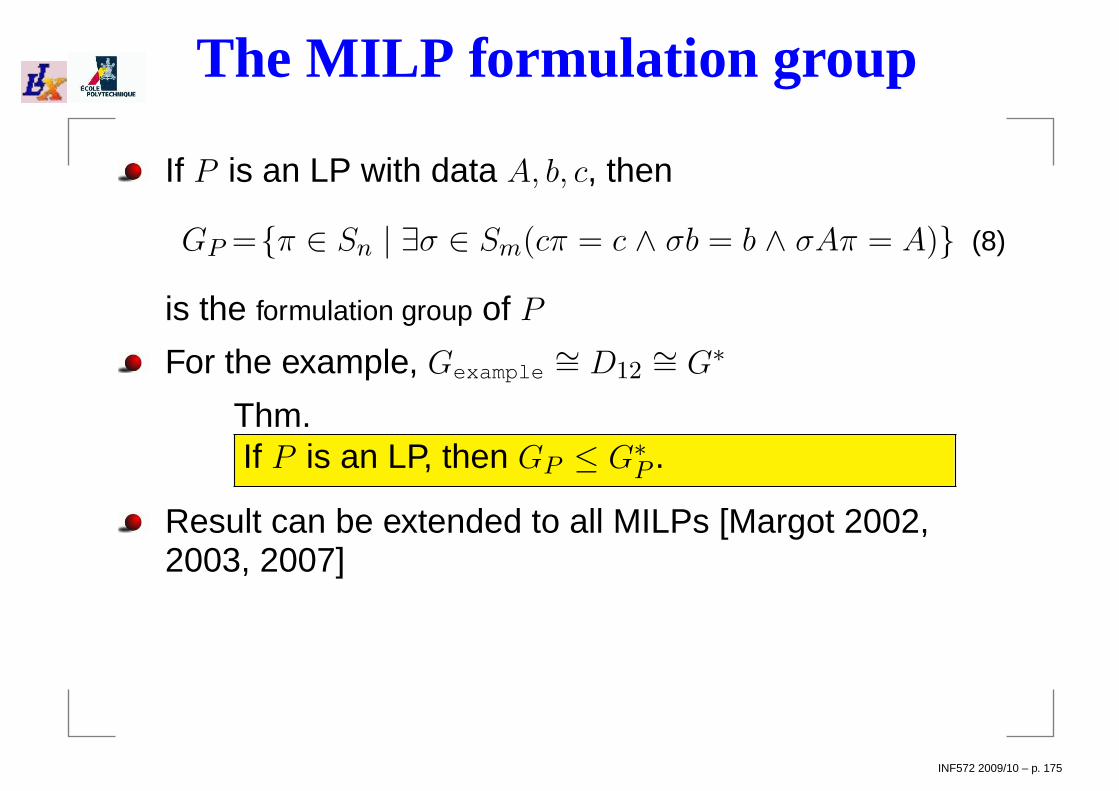
The MILP formulation group

If P is an LP with data A, b, c, then

GP =π ∈ Sn | ∃σ ∈ Sm(cπ = c ∧ σb = b ∧ σAπ = A) (8)

is the formulation group of P

For the example, Gexample∼= D12

∼= G∗

Thm.If P is an LP, then GP ≤ G∗

P .

Result can be extended to all MILPs [Margot 2002,2003, 2007]

INF572 2009/10 – p. 175

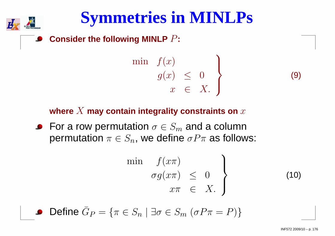
Symmetries in MINLPsConsider the following MINLP P :

min f(x)

g(x) ≤ 0

x ∈ X.

(9)

where X may contain integrality constraints on x

For a row permutation σ ∈ Sm and a columnpermutation π ∈ Sn, we define σPπ as follows:

min f(xπ)

σg(xπ) ≤ 0

xπ ∈ X.

(10)

Define GP = π ∈ Sn | ∃σ ∈ Sm (σPπ = P )INF572 2009/10 – p. 176

A computable definitionEstablishing whether ∀x (σAxπ = Ax) is easy, just look atcomponents of A and σAπ

In general, the statement ∀x (σg(xπ) = g(x) ∧ f(xπ) = f(x)) isundecidable

Assume we have a computable “equality oracle” equal (h1, h2) sothat:

if equal (h1, h2) =true , then ∀x (h1(x) = h2(x))

The converse may not hold

Define GP as GP with = replaced by equal returning true

Can show GP ≤ GP ≤ G∗P

Decision problems:FORMULATION SYMMETRY. Given formulations P, Q and the oracle equal, arethere permutations σ, π such that P = σQπ?

FORMULATION GROUP. Given P and equal, find generators for GP

INF572 2009/10 – p. 177

Equality oracle

Consider the expression DAG representation of g

3∑

i=1xiyi − log(x3/y3)

List of expressions ≡expression DAG sharingvariable leaf nodes

−

+ log

÷×× ×

x1 x2 x3y1 y2 y3

Every function g : Rn → Rm is represented by a DAG whose leafnodes are variables and constants and whose intermediate nodesare mathematical operators

equal (g(x), σg(xπ)) =true if and only if the DAGs rep-resenting g(x) and σg(xπ) are isomorphic

Reduces the FORMULATION SYMMETRY problem to theGRAPH ISOMORPHISM problem

INF572 2009/10 – p. 178

GRAPH ISOMORPHISM

Citation: Babai, Automorphism groups, ismorphism,reconstruction, in Graham, Grötschel, Lovász (eds.),Handbook of Combinatorics, vol. 2

GI is in NP

It is unknown whether it is in P or NP-complete

Solving GI on rooted DAGs is as hard as solving it ongeneral graphs

Solving GI on trees has linear complexity

Our DAGs are “close” to trees, can hope they are nottoo hard for GI testing

INF572 2009/10 – p. 179

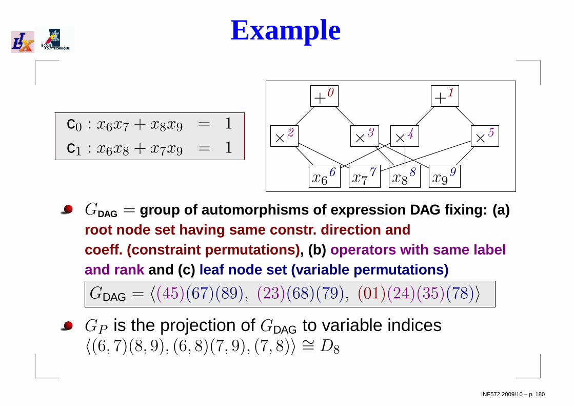
Example

c0 : x6x7 + x8x9 = 1

c1 : x6x8 + x7x9 = 1

x66 x7

7 x88 x9

9

+0

×2 ×3

+1

×4 ×5

GDAG = group of automorphisms of expression DAG fixing: (a)root node set having same constr. direction andcoeff. (constraint permutations) , (b) operators with same labeland rank and (c) leaf node set (variable permutations)

GDAG = 〈(45)(67)(89), (23)(68)(79), (01)(24)(35)(78)〉GP is the projection of GDAG to variable indices〈(6, 7)(8, 9), (6, 8)(7, 9), (7, 8)〉 ∼= D8

INF572 2009/10 – p. 180

Node colorsLet DP = (V,A) be the union of all objective and constraint DAGs inthe MINLP (a.k.a the DAG of P )Colors on the DAG nodes V are used to identify those subsets of nodes which can

be permuted (e.g. variable and operator nodes can’t be permuted)1. Root nodes (i.e. constraints) can be permuted if they have th e same RHS

2. Operator nodes (including root nodes) can be permuted if the y have the

same DAG rank and label; if an operator node is non-commutati ve, then

the order of the children node must be maintained

3. Constant nodes can be permuted if they have the same DAG rank l evel

and value

4. Variable nodes can be permuted if they have the same bounds an d inte-

grality constraints

The relation (u ∼ v ⇐⇒ u, v have the same color) is an equivalence

relation on V (reflexive, symmetric, transitive)∼ partitions V into a disjoint union V/ ∼ of equivalence classes V1, . . . , Vp

INF572 2009/10 – p. 181

MINLP formulation groupsLet P be a MINLP and D = (V ,A) be the DAG of P

Let GDAG be the group of automorphisms of D that fixeach color class in V/ ∼Define φ : GDAG → Sn by φ(π) =projection of π onvariable indices; thenThm.φ is a group homomorphism and Imφ ∼= GP

Hence can find GP by computing Imφ

Although the complexity status (P/NP-complete) of theGRAPH ISOMORPHISM problem is currently unknown,nauty is a practically efficient software for computingGDAG

So now we have GP , how do we write “ P modulo GP ”?

INF572 2009/10 – p. 182

Symmetry-breaking reformulationConsider our first example P :

min x1 + x2

3x1 + 2x2 ≥ 12x1 + 3x2 ≥ 1

x1, x2 ∈ 0, 1

P has G(P ) = (0, 1), (1, 0), G∗ = 〈(1, 2)〉 ∼= C2 andGP = G∗

The orbit GP(0, 1) is the whole of G(P )

We look for a reformulation of P where at least onerepresentative of each orbit is feasible

Let Q be the reformulation of P consisting of P with theadded constraint x1 ≤ x2

We have G(Q) = (0, 1) and G∗ = GQ = 1INF572 2009/10 – p. 183

Breaking orbital symmetries 1Every group G ≤ Sn acting on the variable indices N = 1, . . . , npartitions N into disjoint orbits (all subsets of N )

This follows from the equiv. rel. i ∼ j ⇔ ∃g ∈ G (g(i) = j)

Let Ω be the set of nontrivial orbits (ω ∈ Ω ⇐⇒ |ω| > 1)

Thm. G acts transitively on each of its orbits

This means that ∀ω ∈ Ω ∀i 6= j ∈ ω ∃g ∈ G (g(i) = j)

Applied to MP, if i, j are distinct variable indices belonging to the same orbit

of GP acting on N , then there is π ∈ GP sending xi to xj

Pick x ∈ G(P ); if P is bounded, for all ω ∈ Ω ∃i ∈ ω s.t. xi is acomponent having minimum value over all components of x

By theorem above, ∃π ∈ GP sending xi to xmin ω

Hence x = xπ is s.t. xmin ω is minimum over all other components ofx, and since GP ≤ G∗, x ∈ G(P )

INF572 2009/10 – p. 184

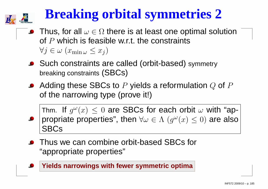
Breaking orbital symmetries 2Thus, for all ω ∈ Ω there is at least one optimal solutionof P which is feasible w.r.t. the constraints∀j ∈ ω (xmin ω ≤ xj)

Such constraints are called (orbit-based) symmetrybreaking constraints (SBCs)

Adding these SBCs to P yields a reformulation Q of Pof the narrowing type (prove it!)

Thm. If gω(x) ≤ 0 are SBCs for each orbit ω with “ap-propriate properties”, then ∀ω ∈ Λ (gω(x) ≤ 0) are alsoSBCs

Thus we can combine orbit-based SBCs for“appropriate properties”

Yields narrowings with fewer symmetric optima

INF572 2009/10 – p. 185

“Appropriate properties”

Notation : g[B](x) ≤ 0 if g(x) only involve variable indices in B

Conditions allowing adjunctions of many SBCs

Thm.Let ω, θ ⊆ 1, . . . , n be such that ω ∩ θ = ∅. Consider ρ, σ ∈GP , and let g[ω](x) ≤ 0 be SBCs w.r.t. ρ,G(P ) and h[θ](x) ≤ 0be SBCs w.r.t. σ,G(P ). If ρ[ω], σ[θ] ∈ GP [ω∪θ] then the systemof constraints g[ω](x) ≤ 0, h[θ](x) ≤ 0 is an SBC system forρσ.

INF572 2009/10 – p. 186

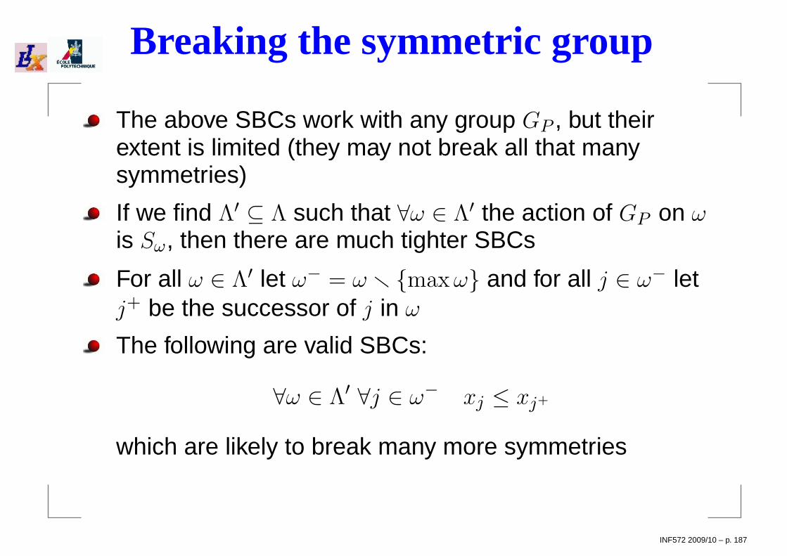
Breaking the symmetric group

The above SBCs work with any group GP , but theirextent is limited (they may not break all that manysymmetries)

If we find Λ′ ⊆ Λ such that ∀ω ∈ Λ′ the action of GP on ωis Sω, then there are much tighter SBCs

For all ω ∈ Λ′ let ω− = ω r max ω and for all j ∈ ω− letj+ be the successor of j in ω

The following are valid SBCs:

∀ω ∈ Λ′ ∀j ∈ ω− xj ≤ xj+

which are likely to break many more symmetries

INF572 2009/10 – p. 187

The final attack on the KNP

INF572 2009/10 – p. 188

Decision KNP

Recall the binary KNP variables are used to count thenumber of spheres

Suggests simply considering whether a fixed number ofspheres can be placed around a central sphere in akissing configuration, or not

This is the decision version of the KNP (dKNP):Given positive integers n, d, can n unit spheres with disjointinterior be placed adjacent to a unit sphere centered at the

origin of Rd?

Should eliminate binary variables, yielding a(nonconvex) NLP, simpler than the original MINLP

In order to find the maximum value for n, we proceed bybisection on n and solve the dKNP repeatedly

INF572 2009/10 – p. 189

The dKNP formulation

Let N = 1, . . . , n; the following formulation P correctlymodels the dKNP:

max 0

∀i ∈ N∑

k∈D

x2ik = 4

∀i ∈ N, j ∈ N : i < j∑

k∈D

(xik − xjk)2 ≥ 4

∀i ∈ N, k ∈ D xik ∈ [−2, 2]

If F(P ) 6= ∅ then the answer to the dKNP is YES,otherwise it is NO

However, solving nonconvex feasibility NLPs isnumerically extremely difficult

INF572 2009/10 – p. 190

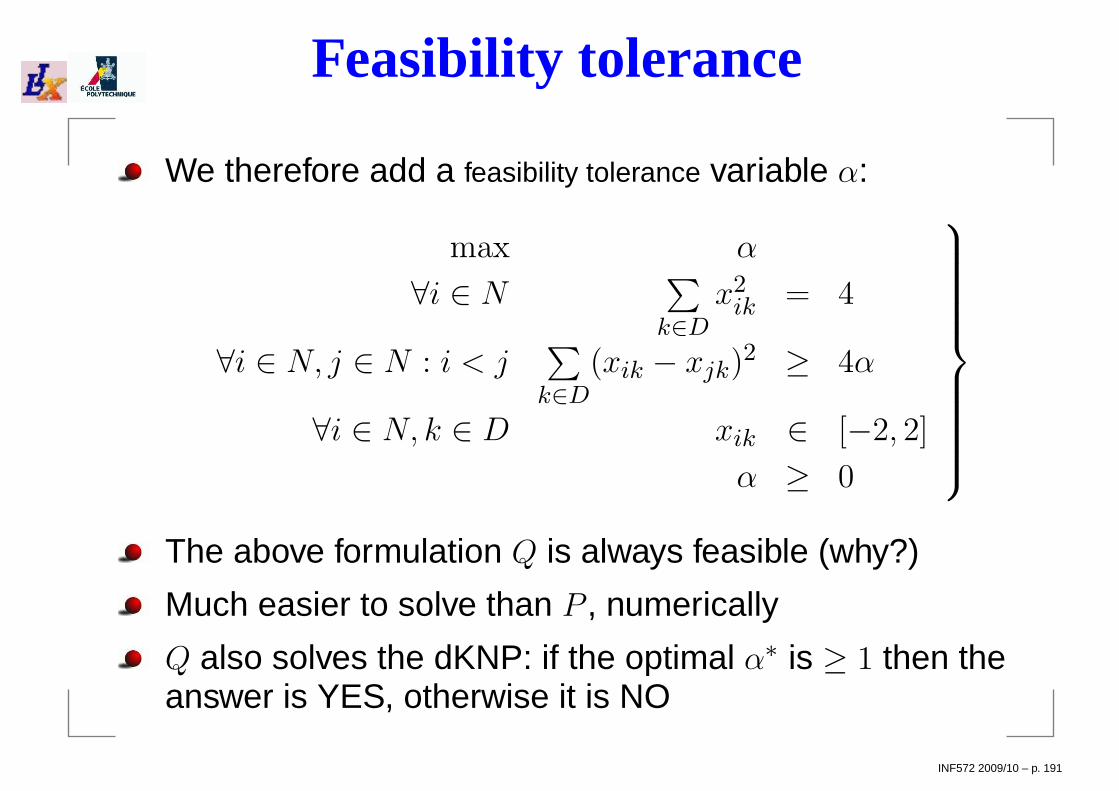
Feasibility tolerance

We therefore add a feasibility tolerance variable α:

max α

∀i ∈ N∑

k∈D

x2ik = 4

∀i ∈ N, j ∈ N : i < j∑

k∈D

(xik − xjk)2 ≥ 4α

∀i ∈ N, k ∈ D xik ∈ [−2, 2]

α ≥ 0

The above formulation Q is always feasible (why?)

Much easier to solve than P , numerically

Q also solves the dKNP: if the optimal α∗ is ≥ 1 then theanswer is YES, otherwise it is NO

INF572 2009/10 – p. 191

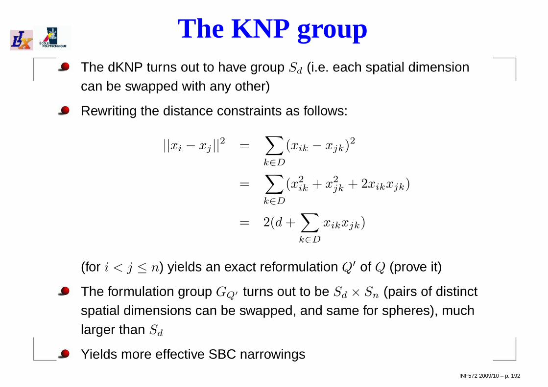
The KNP groupThe dKNP turns out to have group Sd (i.e. each spatial dimensioncan be swapped with any other)

Rewriting the distance constraints as follows:

||xi − xj ||2 =∑

k∈D

(xik − xjk)2

=∑

k∈D

(x2ik + x2

jk + 2xikxjk)

= 2(d +∑

k∈D

xikxjk)

(for i < j ≤ n) yields an exact reformulation Q′ of Q (prove it)

The formulation group GQ′ turns out to be Sd × Sn (pairs of distinctspatial dimensions can be swapped, and same for spheres), muchlarger than Sd

Yields more effective SBC narrowingsINF572 2009/10 – p. 192

Results

Instance Solver Without SBC With SBCD N Time Nodes OI Gap Time Nodes OI Gap

2 6 Couenne 4920.16 516000110150

1 0.04% 100.19 14672 1 0%

2 6 BARON 1200∗ 452596015

1 10% 59.63 2785 131 0%

2 7 Couenne 7200† 465500127220

1 41.8% 7200† 46978038693

1 17.9%

2 7 BARON 10800 25980074419

442 83.2% 16632 693162 208 0%

OI: Iteration where optimum was found†: default Couenne CPU time limit∗: default BARON CPU time limitnodes: total nodes

still on tree

Thus, we finally established by MP that k∗(2) = 6

Actually, solutions for k∗(3) and k∗(4) can be found by using MINLPheuristics (VNS)

INF572 2009/10 – p. 193

The end

INF572 2009/10 – p. 194