Mathematical models of population distribution within a culture group

MATHEMATICAL

COMPUTER MODELLING

PERGAMON Mathematical and Computer Modelling 29 (1999) 57-67

Mathematical Models of Population Distribution Within a Culture Group

H. I. FREEDMAN* Department of Mathematical Sciences, University of Alberta

Edmonton, Alberta, Canada T6G 2Gl

M. SINGH AND A. K. EASTON School of Mathematical Sciences, Swinburne University of Technology

Hawthorn, Victoria, Australia, 3122

I. BAGGS Department of Mathematical Sciences, University of Alberta

Edmonton, Alberta, Canada T6G 2Gl

(Received March 1998; accepted April 1998)

Abstract-Models for the distribution and movement of populations within a culture group are proposed for two and three subcultures. Questions of equilibria, periodic solutions, stability, and persistence versus extinction are considered. @ 1999 Elsevier Science Ltd. All rights reserved.

Keywords-culture group, Equilibria, Logistic, Persistence, Stability.

1. INTRODUCTION

In some previous work [1,2], Baggs and Freedman published several models for the interaction

between several linguistic groups. In these papers, criteria for persistence or extinction of these

groups were obtained.

Bilingualism is a particular aspect of biculturalism. However, biculturalism in general has

certain aspects of complication that are not found in bilingualism. For instance, each cultural

group may have various sects or subcultures associated with it. This is rather common if the

culture is defined by religion. As well, an individual may belong to more than one culture.

There are common perceptions of what defines a cultural group. Some of these are religion,

ethnic background, and geography. One could adopt a general definition of common tradition

(see [3]) as defining such a culture. Having defined cultural group in some manner, for the

purpose of modelling, one could consider a fixed population or a varying population. However

in [4], Dumond argues that growth influences both long term cultural development and change

in social organisation. Hence, our models include varying populations.

Since, to the best of our knowledge, this paper is the first to deal with deterministic cultural

models, we devote this work to the population flow and distribution within a single cultural

group consisting of two or three subcultures, which in the first case one may label as “orthodox”

and “liberal”, and in the second case as “orthodox”, “conservative”, and “liberal”. We leave to

*Author to whom all correspondence should be addressed. This author’s research wss partially supported by the

Natural Sciences and Engineering Research Council of Canada, Grant NSERC A4823.

0895-7177/99/$ - see front matter @ 1999 Elsevier Science Ltd. All rights reserved.

PII: SO8957177(98)00178-Z

Typeset by &&W

58 H. I. FREEDMAN et al.

future work models of a more general makeup within a cultural group and models of interaction

between cultural groups.

In the next section, we will consider the two-subculture model, and in Section 3, the three-

subculture model. In each of these we develop the model, search for equilibria, and discuss

their stabilities. We then touch on the question of whether or not periodic solutions exist and

finally obtain criteria for persistence or nonpersistence (related to extinction) of all subcultures.

Persistence can be given a mathematical formulation (see [S-7]). A population N(t) is said to

(strongly) persist if N(0) > 0 implies that liminf tdoo N(t) > 0. It further uniformly persists if

there exists S > 0 such that liminf tdoo N(t) 2 6, where 6 is independent of N(0) > 0. We use

these definitions throughout the remainder of the paper.

2. THE TWO-SUBCULTURE MODEL

2.1. The Model

We take as our model of twd subcultures interacting with each other and with the population

at large within a given culture to be

fl = wTl(Q) - ~2flh) + Zlfi(Z2) + ClZlr Q(O) = 510 2 0,

22 = z292(z2) - Zlfi(Z2) + ZZfl(4 + E222, zz(O) = z20 L 0, (1)

where . = $. Here xl(t) is the concentration of the liberal subculture and zz(t) is the concentra-

tion of the orthodox subculture at time t > 0. gi(zi) is the specific growth rate of population xi.

Such a growth is deemed necessary in the light of comments in [4]. According to Keyfitz [8],

logistic growth is a reasonable approximation to human population change over a reasonable

length of time. Hence, we suppose that gi(zi) is a generalized form of the logistic (also see [9]).

This translates into the following assumptions on gi(zi):

WI gi(0) > 0, F < 0, there exists Ki > 0

such that gi(Ki) = 0,’ lim gi(si) = -00, i = 1,2. CCi+oo

Ki is the carrying capacity of the environment for the ith population. The last assumption

indicates the consequences (large death rate) of extreme overpopulation.

In any culture, there are forces and influences which one subcultural group exerts on members

of the other to switch subcultures. This is particularly true where there are philosophical or

religious differences between subcultures. This is incorporated in the model by the terms of the

form xifj(xj), i, j = 1,2, i # j. Of course, if any subculture is void of population, there can be

no influence exerted, and the larger the population, the larger the influence. This leads to the

assumptions on fi(zi) that

U-W fi(O) = 0, y > 0, i = 1,2. E

Further, although individuals may switch from liberal to orthodox, there is evidence that a

higher percentage switch from orthodox to liberal. Such evidence is from statistics showing

a general trend of declining church and religious school attendance as well as an increase in

intermarriage in religious cultural groups, for example [IO-121. A s a consequence, we assume

0-3 f2(') > fl(.>.

Finally, there is the matter of the interactions of the subcultures with the community at large.

Individuals may leave or join the cultural group, or in the case of complete isolation (geographic

Population Distribution 59

or cultural) may not interact with the general community at all. The terms of the form c;xi represent this interaction. If ei > 0, there is a net gain to the ith subculture from the general community; if ei < 0, there is a net loss to the general community; if ei = 0, there is no such gain or loss. One usually thinks of the gain or loss as arising from the liberal subculture, but gains and losses are also possible for the other subcultures. For example, the converted may be the greatest zealots.

Finally, so that our model may be treated as a dynamical system, we assume that all functions are so smooth that all solutions to (1) exist, are unique and continuable for all positive time.

Since fi(0) = 0, it is sometimes convenient to write

fi(Xi) = Xihi(Xi)

and assume

P-Y hi(O) 2 07 - h(G) , o

dxi - ’ i = 1,2, h2(.) > h(.).

Then system (1) takes the form

kl = X191(X1) - XlX2h(Xl) + XlX2h2(X2) + 61X1, Xl(O) = X10 > 0,

k2 = X292(X2) - XlX2h2(X2) + XlX2h(Xl) + E2X2r x2(0) = x20 2 0. (2)

Note that solutions with positive initial conditions must remain positive. We now show that the system is dissipative. First note that if we let x = xi + x2, then

i = Xlch(Xl) +x292(22) + ElXl + 6222

= -X +X1(91(X1) + Cl + 1) +x2(92(22) + 62 + 1).

Since limzi,, gi(Xi) = -00, 0 C kfi = SUPo<zi<~ xi(gi(xi)+ei+l) exists. Then if A4 = Mi+M2, we get i L -x + M. Using standard comparison theory gives that

O I Xl(t) + X2(t) I (510 + x20 - M)eet + M,

proving the dissipativity.

2.2. Equilibria

There are four possible equilibria. Clearly, Ee : (0,O) is an equilibrium. To obtain the next two equilibria, we denote by Li, i = 1,2, the unique solutions of

gi(Li) + Ei = 0.

Clearly, Li exist uniquely since gi(O) > 0 and gi(xi) strictly decrease to -oo as xi --) 00. Note that if ei > 0, then Li > Ki; if ci = 0, then Li = Ki; if -gi(O) < ci < 0, then 0 < Li < Ki. From the above, we see that Ei : (LI, 0) and EZ : (0, L2) are equilibria.

There may or may not exist an interior equilibrium which we denote by fi : (&, g2). If fi exists, it must be the solution of the algebraic equations

Xlin(X1) - XlX2h(Xl) + XlX2h2(X2) + ClXl = 0,

X292(X2) - XlX2h2(X2) + XlX2hl(Xl) + E2X2 = 0. (3)

By adding the two equations of (3) and using the second equation, we get the equivalent system

X1&(X1) + ElXl +x292(22) + E2X2 = 0, (4

92(X2) - Xlh2(X2) + Xlh(X1) + f2 = 0. (5)


Figure 1.

Let l? be the curve represented by equation (4). Then r is a closed convex curve which passes

through (0, O), (Ll, O), (0, Lz), and (Ll, L2) (see Figure 1). Let r2 be the curve represented by equation (5). Then fi exists if and only if I?2 intersects I’ at some positive values of (21, ~2).

Consider l72. It also passes through (0, Lz). We now compute

dxs G (O&z)

for both r and r2. We assume throughout that gi(0) + Q > 0. On r,

dxz 91(O) + El !71(0> + El - dx =- > 0,

1 Kwz) g2(L2) + L2&L2> + c2 = - L2@2)

since g:(zi) < 0. On r2,

dxz

z (O&a) =

h2@2) - hi(O) < o

g@2) ’

since hz(L2) > hz(0) > hl(0). H ence, for small positive 21, r2 lies interior to r. If on r2, z2 > 0 for all x1 > 0, then l?z must intersect I’1 and _8? exists. Suppose that there exists zlc > 0 so that

(zlc, 0) lies on l?2. Then if zlc > L1, fi must exist. Further from (5) we have that zlc satisfies

92(O) - %hz(O) + %hl(Zlc) + e2 = 0. (6)

Note that if ,?? exists, then it is unique, for in order to have multiple positive intersections of l?

and r2, we must have by the convexity of I’ that l?z doubles back on itself. But

dx2 hz(s2) - hlZ1) - zlh:bl) - =

dz1 rz ggsz> - ZlMZ2) ’

and, since the denominator is always negative and hence never zero, this cannot occur.

From the above, we have proved the following theorem.

THEOREM 1. Let equation (6) have either

(i) no positive solution zlc, or

(ii) a positive solution zlc such that zlc > Ll.

Then a unique l? exists.


2.3. Periodic Solutions

We now use Dulac’s theorem (see [l]) to show that system (2) has no periodic solutions lying

in the positive quadrant. For completeness we state Dulac’s theorem as Proposition 1.

PROPOSITION 1. Consider the system

kl = &(n, 22),

f2 = F2(m,22). (7)

Let ‘D be a simply connected domain and let F~(z~,Q), i = 1,2 and B(zl,zz) E C2(D). Define

the Dulac function D(q) ~2) by

D(n,zz) = & (B(z1,3~2)J’1(21,~2)) + & (B(zl,z2)J72(Z1,22)) *

Then if D(xl, x2) does not change sign and is not zero on a set of positive measure in D, there

can be no closed path solution of (7) lying entirely in 2).

THEOREM 2. There are no closed path (and hence no periodic) solutions of system (2) lying in

the first quadrant.

PROOF. Let 6 > 0 and let V = {(x1,x2) : XI > 6, 22 > a}. Let

Fl(Zl,XZ) = x191(x1) - XlX2h(Q) + x1zzhz(s2) + ElXl,

F2(21,22) = 2292(22) - qzzh2(s2) + nxzh(x1) + f2X2,

and let

Then,

B(Xl, x2) = x;lx;l.

Dh,x2) = &Wl) + &(BFa)

= x21d(x1) - h’,(a) + $g;(x2) - &(x2).

Since g; < 0, gi < 0, h’, > 0, and hb > 0, D(zI,x~) < 0. Hence, since 6 > 0 is arbitrary, by

Dulac’s theorem the result follows.

2.4. Stability

In order to compute the stability of the various equilibria of system (l), we let M be the

variational matrix about the point (x1,22). Then

wJ’1(~1) +91(x1) --A(%) +4(x2)

-xczfi(51) + f2(52) + El

M= -fi(X2) + x2f&) ~2$7~(~2) + 92(22)

-&(x2) + fl(X1) + E2 1.

Computing M at & : (O,O), we get

M _ go(O) +El 1 0

O- 0 1 gz(O)+ez *

By our assumption gi(Li) + Q = 0, both eigenvalues are positive, and hence, this equilibrium is

unstable.


Computing M at El : (LI, 0), we have that

Mi = Jk?:(Jh) + g1(&) + El -fl(b) + -M(O)

0 I !?2(0)-w~(O)+fl(Jh)+~2 .

Hence,

Mi = h:(b) --h(h) + wgo) . 0 92(O) - Jw#4 + fl@l) + c2 1

The first eigenvalue is negative since Lig:(Li) < 0. Now, consider the second eigenvalue for El. If 92(O) -Li_f~(O)+fi(Li)+cs > 0, then (Li,O) is

a hyperbolic saddle point. If gs(O)-Lrfi(O)+fi(Li)+cs < 0, then (Li,O) is a stable equilibrium.

Computing M at Es : (0, L2) gives

M _ 2-

[

91(O) - J52fi(O) + fi(J52) + Cl 0 * -fi(J52) + Laf;(O) L29@2) + g2(L2) + E2 1 Hence,

M = L?l(O) - J52fi(O) + fi(L2) + 61 0

2

1 -fi(J52) + J52fi(O) L2L$(L2) 1 and the second eigenvalue Lsgi(Ls) is negative.

Now, consider the first eigenvalue for Es, gi(0) - L&(O) + fs(L2) + ~1. By definition, gi(0)

+ ~1 > 0. Also, fs(Ls) - f;(O) > 0. Hence this eigenvalue is positive and so Es : (0, L2) is a

hyperbolic saddle point.

In the case that both El and E2 are saddle points, there must exist an internal equilibrium

which must be unique. Since the system is dissipative, if E exists it must then be globally

asymptotically stable with respect to solutions such that 210 > 0, ~20 > 0.

Note that if xic exists, xic is independent of LI, but does depend on Lp. This implies that if

L1 is sufficiently large for fixed Ls, then E will not exist, El will be asymptotically stable, and

52 will go extinct (see Figure 1).

3. THE THREE SUBCULTURE MODEL

3.1. The Model

In this section, we consider the case where the culture is composed of three subcultures, “or-

thodox”, “conservative”, and “liberal”. This leads to the model

51 = Wl(~1) - z2f1(571) + Qfil(Z2) + ~1x1,

k2 = x292(22) - zlfil(z2) + 22fl(xl) - 23f23(22) + 22f3@3) f c222, (8)

k3 = x393(23) - x2f3(23) + 23f23(22) + ‘53x3,

Xi(O) = ZgJ > 0, i = 1,2,3,

where xi(t) is the concentration of the liberal subculture, 22(t) is the concentration of the conser-

vative subculture, and x3(t) is the concentration of the orthodox subculture. The functions and

constraints in system (8) have analogous interpretations and properties as in system (1). Hence

we assume that

(H5) gi(o) > 0, y < 0, there exists Ki > 0

0 such that gi(Ki) = 0, lim gi(xci) = -00, i = 1,2,3,

zi-‘oo


VW fi(O) = 0, qg > 0, fij(O) = 0, -

42jk2) > 0

dx2 ’ i, j = 1,3,

z

fl(‘) < fil(‘), f23(‘) < f3(*)*

Further, setting

fi(xi) = xih(xi), fij(X2) = X2h2j(x2), i, j = 1,3,

we assume

(H7) hi(O) 2 0, +w - > dXi 0 - ’ h2J0) 2 0 dham 7 > dx2 0 = - ’ i, j 1,3,

hl(.) < h21(*), h23(‘) < h3(‘).

Each ei could be positive, negative, or zero, representing the net interaction of each subculture with the community at large.

3.2. Equilibria and Stability

There is always an equilibrium at the origin Eo : (O,O, 0) and three axial equilibria El :

(LI, O,O), & : (0, L2,0), and E3 : (O,O,L3). There is at least one and up to three planar equilibria. El3 : (Lr , 0, L 3 must exist. El2 : (&,&,O) and E23 : (O,&,fif3) may or may not )

exist. Finally, there may be a positive interior equilibrium of the form E* : (zz, zz,xz). Criteria

for El2 to exist were given in the previous section and similar criteria apply to E23. *

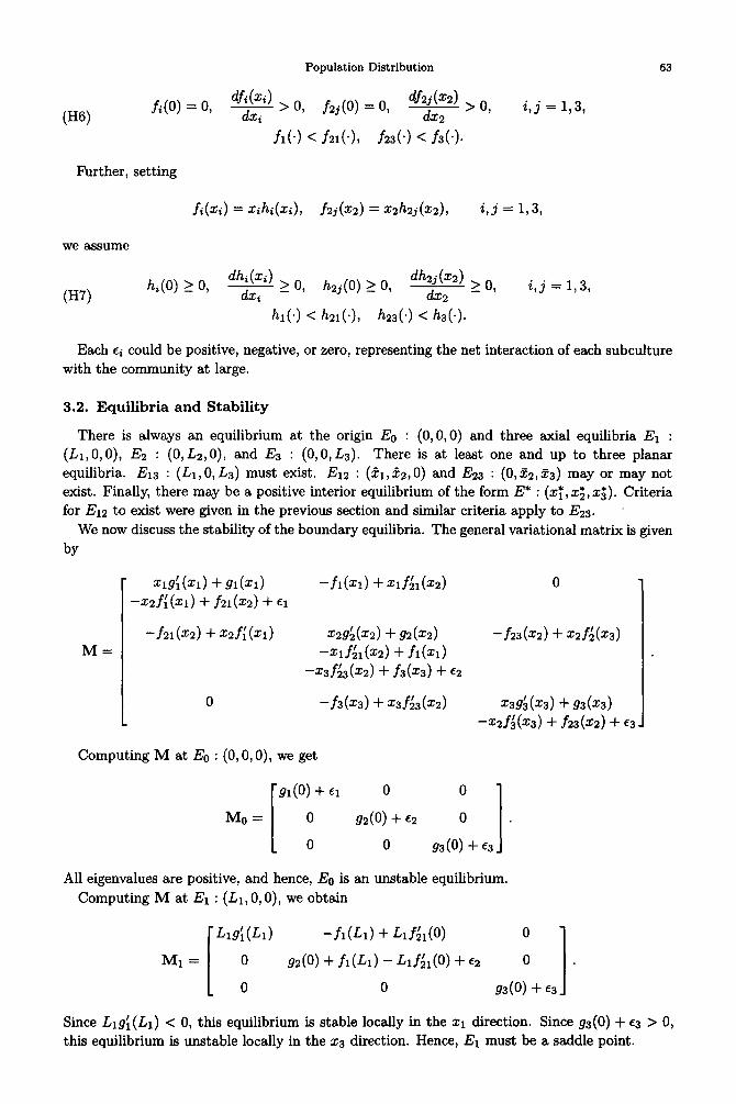
We now discuss the stability of the boundary equilibria. The general variational matrix is given

M=

Xl!d(Xl) +91(x1)

-52t: (Xl) + fil(X2) + El

-f21 (x2) + x2fi (Xl)

0

-h(x1) +x&(x2) 0

x2!$?(x2) +92(x2) -f23(x2) + xZf;(x3)

-x&(x2) + fl(X1)

-x3f;3(x2) + j-3(x3) + c2

-f3(x3) + x3f;3(x2) x39$(x3) +93(x3)

-x2f;(x3) + f23(x2) + c3

Computing M at Eo : (O,O, 0), we get

Mc=

I

91(O) + Cl 0 0

0 92(O) + e2 0 .

0 0 93(O) + 453 1 All eigenvalues are positive, and hence, Es is an unstable equilibrium.

Computing M at El : (Ll,O,O), we obtain

-f1&) + Will(O) 0

92(O) + fl(L1) - W~l(O) + E2 0 .

0 93(O) + e3 I

Since Llgi(LI) < 0, this equilibrium is stable locally in the 21 direction. Since gs(0) + e3 > 0, this equilibrium is unstable locally in the 2s direction. Hence, El must be a saddle point.


Computing M at EZ : (0, Lz, 0), one obtains

- 91(O) - J52fi (0) 0 0

+f21(J52) + El

M2 = -f21(L2) + Lzf;(o) L2!&L2) -f23&2) + Lzf;(o) .

0 0 93(O) - J%(O)

+f23(L2) + ‘53 _

One eigenvalue is Lsgh(L2) < 0. Since Lzg;(Ls) < 0, E2 is stable locally in the 22 direction.

Since 91(O) - L2fi(O) + f21(~52) + ~1 > 0, it is unstable locally in the 51 direction and E2 is a

saddle point.

Computing M at E3 : (O,O, L3), one has

[

91(O) + El 0 0

M3= 0 92(O) - J53f;3(0) + f3(L3) + E2 0 ’

0 -f3(L3) + =53fi3(0) L3gi(L3) I

Since L3g$(L3) < 0, this equilibrium is stable locally in the 2s direction. Since gr(0) + ~1 > 0, it

is unstable locally in the zr direction. Hence, E3 must be a saddle point.

Computing M at El2 : (fr,&,O), we get

&g:(h) + g1(&) --h(h) + C&1(22) 0

-22.f; (21) + fil(22) + 61

-f21(fz) + ?zfi(h) ~29@2) + g2(22) -f23@2) + f2&(0)

M12 = -5&(~2) + h(h)

-23f;3(22) + f3(23) + c2

0

Computing M at El3 : (Ll, 0, Ls), one has

0 93 (0) - 52fi (0)

+f23(*2) + ‘53 4

‘Llg;(Ll) + 57l(Llf + Cl -h(L1) + Ll&(O) 0 7

0 92(O) - We, 0

M13 = +f1(h) - L3fi3(0)

+f3(J53) + E2

0 -f3(L3) + L3fi3(0) L3!A(L3) + L393(L3) + 63-

Computing M at E23 : (0, ~2, ji3), we have

- 91(O) - Z2fiP) 0 0

+f21@2) + El

M23 = -f21(32) + 52fi(O) 32g@2) + g2(f2) -.f23(12) + zZf@3)

--z3f;3@2) + f3(53) + E2

0 -f3(33) + z3f;3@2) ~39@3) + 93(33)

-52f;@3) + f23@2) + ‘53

Setting fi(rci) = zihi(zi), fij(zi) = z$ij(zi), we examine the eigenvalues

(12 = 93(o) - i2h3(0) + 22h23(*2) + f39

&3 = 92(o) - L&21(0) + Llh(&) - L3h23(0) + L3h3(L3) + E2~

<23 = 91(o) - 52h(o) + 52h21@2) + c1.

We note that, 623 > 0 if cl > 0. El2 determines the stability or instability locally in the ~3

direction of E12, t13 locally in the x2 direction of E13, and l& locally in the 21 direction of ET%


3.3. Persistence and Extinction

In general, one may not be able to analyse in detail the dynamics of system (8), or even

determine criteria for the existence of E* by solving the set of algebraic equations obtained by

setting the right-hand side of the equations (8) equal to zero. However, a more fundamental

question can be addressed, namely, when will all three subcultures persist or when will one or

more of them go extinct? Then having addressed this question, a byproduct will be criteria

for E* to exist. In the next theorem we address the persistence versus extinction question.

THEOREM 3.

(a) If any of the following hold:

(i) if El2 exists then [is < 0,

(ii) 613 < 0,

(iii) if E23 exists then 523 < 0,

then system (8) exhibits nonpersistence, i.e., there exists a set of positive measure lying

interior to Rz such that for solutions initiating in this set approach the coordinate plane.

(b) If all of the following hold:

(i) if El2 exists then & > 0,

(ii) 113 > 0,

(iii) if E23 exists then (23 > 0,

then system (8) exhibits persistence.

PROOF OF (a). The proof is immediate since in either case a planar equilibrium is locally stable

in the interior direction.

OUTLINE OF PROOF OF (b). The proof is similar to proofs found in many three-species systems

in ecological modelling (see, for example, [7,13,14]). One first shows, using the Butler-McGehee

Lemma [13], that for solutions with positive initial conditions the origin cannot be part of the

omega limit set. Then one shows the same to be true for the axial equilibria and then finally for

the planar equilibria. Finally, since the only closed, compact invariant sets on the boundary are

equilibria, all solutions are bounded away from the coordinate planes, proving the theorem.

Now we are able to obtain a simple criterion for the existence of E”.

THEOREM 4. If system (8) is persistent, the E’ exists.

PROOF. By the hyperbolicity, isolatedness, and acyclicity of the boundary equilibria, from the

main theorem of [5], system (8) is uniformly persistent. Then from [5], E* must exist.

Note that the above result does not say anything about the uniqueness or stability of E’, nor

does it address the question of periodic solutions.

4. EXAMPLES

To illustrate our results, we take gi(zi) = 1 - xi and hi(~) = hi, hsj(x2) = h2j. Then

system (8) becomes

?I = x1(1 - xl) + (ha - hl)xlxz + ~1~1,

32 = x2(1 - x2) - (h21- h)xlx2 + (h3 - h23)x2x3 + ~2x2,

33 = x3(1 - x3) - (h23 - h3)x2x3 + ~3x3,

xi(o) = xi0 > 0, i = 1,2,3.

From the definition of Li, we see that


which implies that

ci > -1.

The equilibria are as follows. Es : (O,O, 0), El : (1 +ci, O,O), E2 : (O,l+c2,0), E3 : (O,O, l+cs),

and Ers : (1 + cl, 0,l + ~3) are immediate. El2 and E23 may be obtained by solving the two algebraic systems

1+ El - 21 + (h21 - h&2 = 0,

1+ E2 - (hz1 - h&l - z2 = 0,

and

1 + c2 - 22 + (h3 - h23)23 = 0,

1 + E3 - (h23 - h3)Z2 - 23 = 0,

respectively, giving

1+ ei + (h21 - hl)(l + E2) 1+ f2 - (h21 - h)(1+ Cl)

1+ (h21 - h)2 ’ 1+ (h21 - h)2 ,o

>

and

E23 = 0, 1 + 62 + (h3 - h23)(1 + E3) 1 + c3 - @3 - h23)(1 + c2)

1+(h3-h23)2 ’ 1 + (h3 - h23)2 > ’

so that El2 exists if and only if (hzi - hi)(l + ~1) < 1 + 62, and E23 exists if and only if

(ha - h23)( 1 + ~2) < 1 + ~3. Now we compute Eij when they exist, namely,

‘52 = 1 + ‘53 - (h23 - h3) 1 + f2 - (h21 - h)(l + El)

1+ (h21 - h1)2 1 ’ (13 = 1 + e2 - (h21 - h)(l + cl) + (h3 - h23)(1 + f3),

<23 = 1 + cl + (h21 - hl) 1 + 62 f (h3 - h23)(1 + E3)

1 + (h3 - h23)2 1 ’ To illustrate many of the various cases, we take hsr - hi = 1 and h3 - h23 = 1. Then Eis

exists if and only if ~1 < ~2 and E23 exists if and only if ~2 < ~3. Further, if they exist

1 1 cEl2 = 1+ -61 - -Q + 63,

2 2

t13 = 1 - 61 + 62 + E3,

523 2 1 1

= + Cl + -62 + --e3. 2 2

(i> (ii)

(iii)

~1 < ~2 < ~3, both El2 and E23 exist and since ci > -1, all <ij > 0 giving persistence.

cl < ~2 and ~2 > es. Then E23 and hence <23 do not exist. Then if ei = ~3 = 1, ~2 = 0.2,

512 > 0 giving persistence. However, if ei = 0.2, ~2 = 2, es = -0.4, then (12 < 0 causing

2s to locally become extinct.

~1 > ~2 > 63. Then only El3 and 513 exist. If ei = 0.3, ~2 = 0.2, es = 0.1, then (13 > 0 giving persistence. If er = 0.3, ~2 = -0.4, ~3 = -0.5, then 513 < 0 giving extinction of all

populations.


5. DISCUSSION

In this paper, we have made a first attempt to model the distribution of populations within a

given cultural group with two or three interacting subcultures. We have looked at questions of

equilibria, stability, and persistence or extinction of the subcultures.

The persistence versus extinction question to a given cultural group may be the one of particu-

lar interest. The criteria for persistence or extinction are interpretable in terms of the interaction

coefficients and the birth and death parameters. Some of the conclusions are obvious. If birth

rates are high or if the subcultures prove sufficiently attractive to the population at large, persis-

tence is guaranteed. On the other hand, if a given subculture becomes very unpopular so that the

rate of net loss to other subcultures or the community at large exceeds the birth rate, extinction

will occur.

In both our models, persistence of all subcultures implies the existence of a positive steady

state. In the two-subculture model, this steady state was shown to be globally asymptotically

stable. We can make no such claim about the steady state in the three-subculture model. There

may even exist periodic solutions in this case.

In future work, we will attempt to extend our results to an n-subculture model and attempt to

account for spatial distributions its well as temporal. As well, we will re-examine the persistence

question in the light of several interacting cultures, each with various subcultures.

REFERENCES

1. I. Baggs and H.I. Freedman, A mathematical model for the dynamical interaction between a unilingual and bilingual population: Persistence versus extinction, J. Math. Biology 16, 51-75 (1990).

2. I. Baggs and H.I. Freedman, Can the speakers of a dominated language survive as unilinguals?: A mathematical model for bilingualism, Ma&l. Comput. Modelling 18 (5), 9-18 (1993).

3. J.A. Soares, A reformulation of the concept of tradition, In Rethinlcing the Sociology of Culture, (Edited by J.H. Stanfield, II); Int. J. Sociology and Social Policy 17, 6-21 (1997).

4. D.E. Dumond, Population growth and real culture change, In Introductory Readings on Sociological Con- cepts, Methods, and Data, (Edited by M. Abrahamson), pp. 118-137, Van Nostrand, New York, (1969).

5. G.J. Butler, H.I. F’reedman and P. Waltman, Uniformly persistent systems, Proc. Amer. Math. Sot. 96, 425-429 (1986).

6. H.I. Reedman and P. Moson, Persistence definitions and their connections, Proc. Amer. Math. Sot. 109, 1025-1033 (1990).

7. H.I. needman and P. Waltman, Persistence in a model of three competitive populations, Math. Biosci. 73, 89-101 (1985).

8. N. Keyfitz, Introduction to the Mathematics of Populations with Revisions, Addison-Wesley, (1977). 9. H.I. Freedman, Deterministic Mathematical Models in Population Ecology, Marcel Dekker, New York,

(1980). 10. G.C. Oosthuizen, J.C. Goetzee, J.W. de Gruchy, J.H. Hofmeyr and B.C. Lategan, Religion, Intergroup

Relations and Social Change in South Africa, Greenwood Press, New York, (1988). 11. D.M. Kelley, Why Conservative Churches are Growing, Mercer University Press, Macon, GA, (1986). 12. H. Mol, Religion in Australia, Thomas Nelson, Sydney, (1971).

13. H.I. F’reedman and P. Waltman, Persistence in models of three interacting predator-prey populations, Math. Biosci. 68, 213-231 (1984).

14. R. Kumar and H.I. Freedman, A mathematical model of facultative mutualism with populations interacting in a food chain, Math. Biosci. 97, 235-261 (1989).

Documents

Mathematical models of population distribution within a culture group