Mathematical Models And Statistical Analysis of Credit ... · Mathematical Models And Statistical Analysis of Credit Risk Management Tianfeng Hou Mathematical Institute, Universiteit

Mathematical Models And Statistical Analysis ofCredit Risk Management

THESIS

submitted in partial fulfillment of therequirements for the degree of

MASTER OF SCIENCEin

MATHEMATICS AND SCIENCE BASED BUSINESS

Author : Tianfeng HouSupervisor : Dr.Onno Van Gaans2nd corrector : Prof.Richard Gill3nd corrector : Dr.Flora Spieksma

Leiden, The Netherlands, August 27, 2014

Mathematical Models And Statistical Analysis ofCredit Risk Management

Tianfeng Hou

Mathematical Institute, Universiteit LeidenP.O. Box 9500, 2300 RA Leiden, The Netherlands

August 27, 2014

Abstract

This thesis concerns mathematical models and statistical analysisof management of default risk for markets, individual obligors,and portfolios. Firstly, we consider to use CPV model to estimatedefault rate of both Chinese and Dutch credit market. It turns outthat our CPV model gives good predictions. Secondly, we studythe KMV model, and estimate default risk of both Chinese andDutch companies based on it. At last, we use two mathemati-cal models to predict the default risk of investors’ entire portfolioof loans. In particular we consider the influence of correlations.Our models show that correlation in a portfolio may lead to muchhigher risks of great losses.

Contents

1 Introduction 11.1 How to define the loss . . . . . . . . . . . . . . . . . . . . . . 1

1.1.1 The loss variable . . . . . . . . . . . . . . . . . . . . . 11.1.2 The expected loss . . . . . . . . . . . . . . . . . . . . . 21.1.3 The unexpected losses . . . . . . . . . . . . . . . . . . 21.1.4 The economic capital . . . . . . . . . . . . . . . . . . . 3

2 How To Model The Default Probability 52.1 General statistical models . . . . . . . . . . . . . . . . . . . . 5

2.1.1 The Bernoulli Model . . . . . . . . . . . . . . . . . . . 52.1.2 The Poisson Model . . . . . . . . . . . . . . . . . . . . 6

2.2 The CPV Model and KMV Model . . . . . . . . . . . . . . . . 72.2.1 Credit Portfolio View . . . . . . . . . . . . . . . . . . 72.2.2 The KMV-Model . . . . . . . . . . . . . . . . . . . . . 8

3 Use CPV model to estimate default rate of Chinese and Dutchcredit market 153.1 Use CPV model to estimate default rate of Chinese credit

market . . . . . . . . . . . . . . . . . . . . . . . . . . . . . . . 153.1.1 Macroeconomic factors and data . . . . . . . . . . . . 153.1.2 Model building . . . . . . . . . . . . . . . . . . . . . . 193.1.3 Calculating the default rate . . . . . . . . . . . . . . . 25

3.2 Use CPV model to estimate default rate of Dutch credit market 263.2.1 Macroeconomic factors and data . . . . . . . . . . . . 263.2.2 Model building . . . . . . . . . . . . . . . . . . . . . . 263.2.3 Calculating the default rate . . . . . . . . . . . . . . . 32

4 Estimation Default Risk of Both Chinese and Dutch Compa-nies Based on KMV Model 334.1 Use KMV model to evaluate default risk for CNPC and Sinopec

Group . . . . . . . . . . . . . . . . . . . . . . . . . . . . . . . . 33

iv

Version of August 27, 2014– Created August 27, 2014 -

CONTENTS v

4.2 Use KMV model to evaluate default risk for Royal DutchShell and Royal Philips . . . . . . . . . . . . . . . . . . . . . . 40

5 Prediction of default risk of a portfolio 435.1 Two models . . . . . . . . . . . . . . . . . . . . . . . . . . . . 43

5.1.1 The Uniform Bernoulli Model . . . . . . . . . . . . . . 445.1.2 Factor Model . . . . . . . . . . . . . . . . . . . . . . . . 44

5.2 Computer simulation . . . . . . . . . . . . . . . . . . . . . . . 495.2.1 Simulation of the Uniform Bernoulli Model . . . . . . 495.2.2 Simulation of the Factor Model . . . . . . . . . . . . . 51


v

Chapter 1Introduction

Credit risk management is becoming more and more important in today’sbanking activity. It is the practice of mitigating losses by understandingthe adequacy of both a bank’s capital and loan loss reserves to any giventime. In simple words, the financial engineers in the bank need to createa capital cushion for covering losses arising from defaulted loans. Thiscapital cushion is also called expected loss reserve[2]. It is important fora bank to have good predictions for its excepted loss. If a bank keepsreserves that are too high, than it misses profits that could have been madeby using the money for other purposes. If the reserve is too low, the bankmust unexpectedly sell assets or attract capital, probably leading to a lossor higher costs. Mathematical models are used to predict expected losses.Before we discuss various ways of credit risk modeling we will first lookat several definitions.

1.1 How to define the loss

1.1.1 The loss variable

Let us first look at one obligor. By definition, the potential loss of anobligor is defined by a loss random variable

L = EAD× LGD× L with L = 1D, P(D) = DP,

where the exposure at default (EAD) stands for the amount of the loan’sexposure in the considered time period, the loss given default (LGD) is


1

2 Introduction

a percentage, and stands for the fraction of the investment the bank willlose if default happens.(DP) stands for the default probability.D denotesthe event that the obligor defaults in a certain period of time(most oftenone year),and P(D)denotes the probability of the event D.Default rate is the rate at which debt holders default on the amount ofmoney that they owe. It is often used by credit card companies whensetting interest rates, but also refers to the rate at which corporations de-fault on their loans. Default rates tend to rise during economic downturns,since investors and businesses see a decline in income and sales while stillrequired to pay off the same amount of debt. So If we invest in debt wewant to know or minimize the risk of default.

1.1.2 The expected loss

The expected loss (EL) is the expectation of the loss variable L. The defini-tion is

EL = E[L] If EAD and LGD are constants= EAD× LGD×P(D)

= EAD× LGD× DP

This formula also holds if EAD and LGD are the expectations of some un-derlying random variables that are independent of D.

1.1.3 The unexpected losses

Then we turn to portfolio loss. As we discussed before the financial en-gineers in the bank need to create a capital cushion for covering lossesarising from defaulted loans.A cushion at the level of the expected losswill often not cover all the losses. Therefore the bank needs to prepare forcovering losses higher than the expected losses, sometimes called the un-expected losses.A simple measure for unexpected losses is the standard deviation of theloss variable L.

UL =√

V[L] =√

V[EAD× SEV × L]

2


1.1 How to define the loss 3

Where, the SEV is the severity of loss which can be considered as a randomvariable with expectation given by the LGD.

1.1.4 The economic capital

It is not the best way to measure the unexpected loss for the risk capital bythe standard deviation of the loss variable, especially if an economic crisishappens. It is very easy that the losses will go far beyond the portfolio’sexpected loss by just one standard deviation of the portfolio’s loss.It is better to take into account the entire distribution of the portfolio loss.Banks always estimate the so-called economic capital.For instance, if a bank wants to cover 95 percent of the portfolio loss, theeconomic capital equals the 0.95 th quantile of the distribution of the port-folio loss, where the qth quantile of a random variable LPF is defined as

qα = inf{q > 0 | P[LPF ≤ q] ≥ α}.

The economic capital (EC) is defined as the α - quantile of the portfolio lossLPF minus the expect loss of the portfolio,

ECα = qα − ELPF.

So if the bank wants to cover 95 percent of the portfolio loss, and the levelof confidence is set to α =0.95, then the economic capital ECα can coverunexpected losses in 9,500 out of 10,000 years, if we assume a planninghorizon of one year.


3

Chapter 2How To Model The DefaultProbability

2.1 General statistical models

2.1.1 The Bernoulli Model

In statistics, if an experiment only has two future scenarios, A or A, thenwe call it a Bernoulli experiment. In our default-only case,every coun-terparty either defaults or survives. This can be expressed by Bernoullivariables

Li ∼ B(1; pi), i.e., Li =

{1 with probability pi,0 with probability 1− pi.

Next, we assume the loss statistics variables L1, ..., Lm are independent, andregard the loss probabilities as random variables P = (P1, ..., Pm) ∼ F withsome distribution function F with support in[0,1]m,

Li | Pi = pi ∼ B(1; pi), (Li | P = p)i=1,...,m independent.

The joint distribution of the Li is then determined by the probabilities

P[L1 = l1, ..., Lm = lm] =∫[0,1]m ∏n

i=1 plii (1− pi)

1−li dF(p1, ..., pm),


5

6 How To Model The Default Probability

where li ∈ {0,1}. The expectation and variance are given by

E[Li] = E[Pi], V[Li] = E[Pi](1−E[Pi]) (i = 1, ...,m).

The covariance between single losses obviously equals

Cov[Li, Lj] = E[Li, Lj]−E[Li]E[Lj] = Cov[Pi, Pj].

The correlation in this model is

Corr[Li, Lj] =Cov[Pi,Pj]√

E[Pi](1−E[Pi])√

E[Pj](1−E[Pj]).

2.1.2 The Poisson Model

An interpretation if the loss statistics for this model can be that there arem groups of obligors, such that the obligors in each group have the samedefault rate. L′i is the number of obligors in default in group i. This can beexpressed by Possion Model.The Poisson frequency function with parameter λ(λ > 0) is

P{X = k} = λke−λ

k! , k = 0,1,2, ....

Now the loss statistics vecotr L′ = (L′1, ..., L′m) of Poisson random variablesL′i ∼ Pois(Λi), where Λ = (Λ1, ...,Λm) is a random vector with some distri-bution fuction F with support in[0,1]m,

Li | Λi = λi ∼ Pois(λi), (L′i | Λ = λ)i=1,...,m independent.

The joint distribution of the L′i is then determined by the probabilities

P[L′1 = l′1, ..., L′m = l′m] =∫[0,∞]m e−(λ1+...+λm) ∏m

i=1λ

l′ii

l′i !dF(p1, ..., pm),

where li ∈ {0,1,2...}. The expectation and variance are given by

E[L′i] = E[Λi], V[L′i] = V[Λi] + E[Λi]. (i = 1, ...,m).

The covariance Cov[L′i, L′j] = Cov[Λi,Λj]. And the correlation between de-faults is

Corr[L′i, L′j] =Cov[Λi,Λj]√

V[Λi]+E[Λi]√

V[Λj]+E[Λj].

6


2.2 The CPV Model and KMV Model 7

2.2 The CPV Model and KMV Model

2.2.1 Credit Portfolio View

Credit Portfolio View(CPV)[3] is based upon the argument that defaultand migration probabilities are not independent of the business cycle. CPVcalls any migration matrix observed in a particular year a conditional mi-gration matrix, and the average of conditional migration matrices in a lotof years will give us an unconditional migration matrix. The idea is thatthe migration probabilities are conditional on the economic situation inthat particular year. The economic situation is assumed to be approxi-mately cyclic and therefore its effect is averaged out over a lot of years.During boom times default probabilities run lower than the long termaverage that is reflected in the unconditional migration matrix; and con-versely during recessions default probabilities and downward migrationprobabilities run higher than the longer term average. This effect is moreamplified for speculative grade credits than for investment grade as thelatter are more stable even in tougher economic situations.This adjustment to the migration matrix is done by multiplying the uncon-ditional migration matrix by a factor that reflects the state of the economy.If M be the unconditional transition matrix, then Mt = (rt − 1)A + M isthe Conditional transition matrix. How do we derive the factor rt?Here A = aij is a suitable matrix st. aij ≥ 0 for i < j and aij ≤ 0 for i > jThe factor rt is just chosen to be the conditional probability of default inperiod t divided by the unconditional (or historical) probability of default.This is expressed as follows:

rt =PtP ,

where Pt is the conditional probability of default in period t, and P is theunconditional probability.Now Pt itself is modelled as a logistic function of an index value Yt,

11+exp(−Yt)

The index Yt is derived using a multi-factor regression model that consid-ers a number of macro economic factors,

Yt = w0 + ∑Kk=1 wkXk,t + εt,


7


where Xk,t are the macroeconomics factors at time t, wk are coefficients ofthe corresponded macroeconomics factors, w0 is the intercept of the linearmodel, and εt is the residual random fluctuation of Yt

2.2.2 The KMV-Model

The KMV-Model is a well-known industry models.[1] The idea of it isbased on whether the firm’s asset values will fall below a certain criticalthreshold or not. Let Ai

t denote the asset value of firm i ∈ 1, ,m If after aperiod of time T the firm’s asset value Ai

T is below this threshold Ci thenwe say the firm is in default. Otherwise the firm survived the consideredtime period. We can represent this model in a Bernoulli type model. In-deed, consider the random variable Li defined by

Li = 1{A(i)T <Ci}

. This random variable has a Bernoulli distribution.

B(1;P[A(i)T < Ci]) (i = 1, ...,m)

The classic Black-Scholes-Merton models[9] gives a model for the firm’sasset value.

A(t) = Cexpαt+θW(t),

Where C > 0 is constant, α,θ are constant and W is a Brownian motion.The logarithmic return over time T is then:

logA(T)− logA(0)= logC + αT + θW(T)− (logC + 0)= αT + θW(T).

Where θW(T) ∼ N(0, T)The term θT is deterministic and can be absorbed in the threshold, so with-out loss of generality we can take α = 0. Further, we will think of therandom part as consisting if two separate parts: one determined by theeconomic situation and on being specific for the individual obligor. Thuswe arrive at the following formula for the (logarithmic) asset return at timeT:

ri = βiφi + εi (i = 1, ...m).

8



Here,φi is called the composite factor of firm i which is a standard nor-mally distributed random variable describing the state of the economicenvironment of the firm. βi is the sensitivity coefficient, which capturesthe linear correlation of ri and φi.The normal random variable εi standsfor the residual part of ri, it means that the return ri differs from the pre-diction βiφi based on the economic situation by an error εi, which is calledthe idiosyncratic part of the return.

We rescale the (logarithmic) asset value return to become a standard nor-mal random variable,

ri =ri−E[ri]

V[ri](i = 1, ...m).

With the coefficient Ri defined by

R2i =

β2i V[φi]

V[ri](i = 1, ...m)

and with the same sign as βi we get a representation

ri = Riφi + εi (i = 1, ...m).

Here Ri is given above,φi means the company’s composite factor,and εi isthe idiosyncratic part of the company’s asset value log-return.Observe that

ri ∼ N(0,1), Φi ∼ N(0,1), and εi ∼ N(0,1− Ri2).

As in the Bernoulli Model, the joint distribution of the Li is then deter-mined by the probabilities

P[L1 = l1, ..., Lm = lm] =∫[0,1]m ∏n

i=1 plii (1− pi)

1−li dF(p1, ..., pm).

Here what we should get clear is the distribution function F which is stilla degree of freedom in the model. The event of default of firm i at time Tcorresponds to ri < ci. This is equivalent to

εi < ci − Riφi.


9


Denoting the one-year default probability of obligor i by pi,we havepi =P[ri < ci]. As ri ∼ N(0,1),we get

ci = N−1[ pi] (i = 1, ...m),

Here N[�] denotes the CDF(cumulative distribution function) of the stan-dard normal distribution. We can easily replace εi by a standardized nor-mal random variable εi by means of

εi <N−1[ pi]−RiΦi√

1−Ri2

, εi ∼ N(0,1).

Because of εi ∼ N(0,1), the one-year default probability of obligor i condi-tional on the factor Φi can be represented

pi(φi) = N[N−1[ pi]−Riφi√1−Ri

2] (i = 1, ...m),

Finally, If we assume that the distribution function F is that of a multivari-ate normal distribution, then we can express it as

F(p1, ..., pm) = Nm[p1−1( p1), ..., pm

−1( pm);Γ],

Where Nm[�;Γ] denotes the cumulative centered Gaussian distribution withcorrelation matrix Γ, and Γ means the asset correlation matrix of the log-returns ri.In the computations above, we have assumed that firm i is in default attime T precisely when its asset value at time T is below a certain thresh-old. If T is the maturity time of the debt, it is more realistic to assume thatfirm i is in default at time T if at some moment t between 0 and T its assetvalue has been below the threshold. In that case, one can use the theoryof option pricing for the classic Black-Scholes-Merton mode, as is brieflyreviewed next.

The process of KMV model

The process of KMV model can be divided into 4 steps.The first step is: Estimate the company’s asset value and its volatility fromthe company’s stock market, value of volatility of stock price and liabili-ties book value. Generally, since equity can be viewed as a call potion onthe firm’s assets and the volatility of a firm’s equity value will reflect the

10



leverage adjusted volatility of its underlying assets, we have in generalform:

E = f (V, B, r,σv, τ)

and,σs = g(σv)

Here,E is the asset value of the firm,V is the market value of the company,Bis the price for the loan,r is the interest rate,σv is the volatility of assetvalue.τ is put option expiration date.N(d) is the Cumulative distributionprobability function. The bars denote values that are directly measurable.Since we have two equations and to unknowns(V,σv), σs is the volatilityof market value. We may expect to be able to solve the equations.More specifically, According to the relationship between the classic Black-Scholes-Merton model, put option valuation models and default options,

E = V × N(d1)− B× e−rt × N(d2)

d1 =ln(V

B ) + (r + 12 × σ2

v )τ

σv√(τ)

d2 = d1 − σv

√(τ)

According to the relationship between the observable fluctuations in themarket value of the corporate and non-observable fluctuations in the valueof assets of the company we have equations:

σs = (V × N(d1)× σv

E)

We use a continuous iterative method will be able to find V and σv.The second step: Find the default point.The default happens when the value of the firm falls below”default point”.According to the studies of the KMV, some of the companies will not de-fault while their firm’s asset reach the level of total liabilities due to thedifferent debt structure. Thus DPT is somewhere between total liabilitiesand current liabilities, as below:

DPT = SL + αLL,06 α6 1

Under a large of empirical investigation, KMV found violations occurredmost frequently if a company’s value is greater than the critical point if the


11


critical point is taken to be equal to the short-term liabilities plus half oflong-term liabilities[10].

DPT = SL + 0.5LL

HereDPT is the default point,SL is the short-term liabilities, LL is the long-term liabilities.The Third step: find the default-distance(DD).The default-distance(DD) is the number of standard deviations betweenthe mean of asset value’s distribution,and the default point. After we getthe implied V, σv and the default point, the default-distance DD can becomputed as follows:

DD =E(V)− DPE(V)× σv

The Fourth step: Estimate the company’s expected default probability(EDF)The Expected default probability (EDF) is determined by mapping thedefault distance (DD) with the expected default frequency.As the firm’s asset value of Merton model is normally distributed, expecta-tion the E(V) is V0 expu t, which is log-normally distributed. Thus the DDexpressed in unit of asset return standard deviation at the time horizon Tis

DD =ln( VA0

DPTT) + (µ− 0.5σ2

A)T

σv√

T

Here VA0 is the current market value of the assets, DPTT is the defaultpoint at time horizon T, µ is the expected annual return on the firm’sassets,σA is the annualized asset volatility.So the corresponding theoretical implied default frequency (EDF) at oneyear interval is

EDFTheoretical = N(−ln( VA0

DPTT) + (µ− 0.5σ2

A)T

σv√

T) = N(−DD).

12



The asset value is not exactly normally distributed in practice. Based onthe one-to-one mapping relations between the default distancesDD andthe expected default frequency(EDF), the length of the distance to a cer-tain extent reflects the company’s credit status,and thus evaluates the levelof competitiveness of the enterprise.


13

Chapter 3Use CPV model to estimate defaultrate of Chinese and Dutch creditmarket

In this chapter I want to use the CPV model as described in Section 2.2.1 toestimate the default rate(DR) of Chinese and of the Dutch credit market. Iwill use real world data of the Chinese joint-equity commercial bank andthe Dutch national bank.

3.1 Use CPV model to estimate default rate ofChinese credit market

3.1.1 Macroeconomic factors and data

In CPV model macroeconomic factors drive the default rate. Typical candi-dates for macroeconomic factors are Consumer Price Index(CPI),financialexpenditure, urban disposable incomes, Business Climate Index,interestrate, Gross Domestic Product(GDP),and other variables reflecting the macroe-conomy of a country.

In my case study I choose Consumer Price Index(CPI), unemploymentrate, financial expenditure, urban disposable incomes, Fixed asset invest-ment price index, money supply, Business Climate Index,interest rate, GrossDomestic Product(GDP), and the growth rate of GDP to be the macroeco-nomic factors.


15

16 Use CPV model to estimate default rate of Chinese and Dutch credit market

A consumer price index (CPI) measures changes in the price level of a mar-ket basket of consumer goods and services purchased by households.Theannual percentage change in a CPI is used as a measure of inflation.. Inmost countries, the CPI is one of the most closely watched national eco-nomic statistics.

Unemployment (or joblessness) occurs when people are without work andactively seeking work. The unemployment rate(UR) is a measure of theprevalence of unemployment and it is calculated as a percentage by divid-ing the number of unemployed individuals by all individuals currently inthe labor force. During periods of recession, an economy usually experi-ences a relatively high unemployment rate.

In National Income Accounting, government spending, financial expen-diture(FE), or government spending on goods and services includes allgovernment consumption and investment but excludes transfer paymentsmade by a state. It can reflect the strength of the government finance andthe future direction of the national economy.

Disposable income(DI) is total personal income minus personal currenttaxes.

Fixed asset investment price index(FAIPI) reflects the trend and degreeof changes in prices of investment in fixed assets. It is calculated as theweighted arithmetic mean of the price indices of the three components ofinvestment in fixed assets (the investment in construction and installation,the investment in purchases of equipment and instrument,and the invest-ment in other items).

Money supply(MS) is the total amount of monetary assets available in aneconomy at a specific time.

Business climate index(BSI) is the index of general economic environmentcomprising of the attitude of the government and lending institutions to-ward businesses and business activity, attitude of labor unions toward em-ployers, current taxation regimen, inflation rate, and such.

Interest rate is the rate at which interest is paid by a borrower (debtor)for the use of money that they borrow from a lender (creditor).

Grpss domestic product is defined by OECD as ”an aggregate measure

16


3.1 Use CPV model to estimate default rate of Chinese credit market 17

of production equal to the sum of the gross values added of all residentinstitutional units engaged in production (plus any taxes, and minus anysubsidies, on products not included in the value of their outputs.

MY Preliminary dataI using time series data on a quarter base over the years 2009-2013. TheChinese joint-equity commercial bank do not have the united definition ofdefault, instead they uses five-category assets classification for the mainmethod for risk management. Comparing the definition of the probabil-ity of the non-performing loan in five-category assets classification andthe default rate,they are similar. So I choose the probability of the non-performing loan to be the default rate. The data of probability of the non-performing loan is from the official website of China Banking RegulatoryCommission,(http://www.cbrc.gov.cn/index.html)[15].The data of all the macroeconomic factors is from the official website ofNational Bureau Of Statistics Of China,(http://www.stats.gov.cn/)[14].

Table 3.1: All of the required data

DR CPI GDP Growth UR FE DI FAIPI APR MS BSI1.17% 100.03 69816.92 6.6% 4.3% 12810.90 4833.90 98.80 2.3% 502156.67 105.601.03% 99.06 78386.68 7.5% 4.3% 16091.70 4022.00 96.10 2.3% 552553.64 115.900.99% 98.83 83099.73 8.2% 4.3% 16300.20 4117.40 96.40 2.3% 578402.38 124.400.95% 99.10 109599.48 9.2% 4.3% 31097.13 4201.40 99.00 2.3% 597157.51 130.600.86% 101.90 82613.39 12.1% 4.1% 14330.00 5308.00 101.90 2.3% 637209.67 132.900.80% 102.50 92265.44 11.2% 4.1% 19481.40 4449.10 103.60 2.3% 652611.44 135.900.76% 102.80 97747.91 10.7% 4.1% 20693.60 4576.70 103.50 2.5% 686009.97 137.900.70% 103.16 128886.06 10.4% 4.1% 35070.00 4775.60 105.40 2.5% 711989.19 138.000.70% 104.93 97479.54 9.8% 4.1% 18053.60 5962.80 106.50 3.0% 742715.52 140.300.60% 105.23 109008.57 9.7% 4.1% 26381.50 5078.70 106.70 2.9% 767204.88 137.900.60% 105.60 115856.56 9.5% 4.1% 25045.50 5259.40 107.30 3.5% 780394.05 135.600.60% 105.50 150759.38 9.3% 4.1% 39521.40 5508.90 105.70 3.3% 831304.67 127.800.63% 104.07 108471.97 7.9% 4.1% 24118.10 6796.30 102.30 3.3% 872878.60 127.300.65% 103.50 119531.12 7.7% 4.1% 29774.90 5712.20 101.60 3.3% 904881.34 126.900.70% 102.93 125738.46 7.6% 4.1% 30226.30 5918.10 100.20 3.0% 929218.58 122.800.72% 102.67 165728.55 7.7% 4.1% 41592.70 6138.10 100.30 3.0% 951798.71 124.400.77% 102.33 118862.08 7.7% 4.1% 27036.70 7427.30 100.20 3.0% 1008862.82 125.600.80% 102.40 129162.37 7.6% 4.1% 32677.30 6221.80 99.90 3.0% 1043041.58 120.600.83% 102.47 139075.79 7.7% 4.1% 31818.30 6519.90 100.10 3.0% 1063615.98 121.500.86% 102.60 181744.97 7.7% 4.1% 48211.70 6786.00 100.90 3.0% 1085336.12 119.50

Data adjusted by CPI Index and after seasonal adjustmentIn the data table above ,financial expenditure, urban disposable incomes,money supply, Gross Domestic Product(GDP),will influence by the CPIIndex.So If we want to analysis these data, we will calculate the CPI Indexfirst,and adjusted these factors by it.For calculating the CPI Index,we use the CPI of 1 quarter 2009 as base.(theCPI Index of 1 quarter 2009 is 1)

CPIIn = CPIn × CPIn−1 × ...× CPIbase


17


After the data adjusted by CPI Index, we found that several macroeco-nomic factors such as financial expenditure, urban disposable incomes,Fixed asset investment price index, Gross Domestic Product(GDP), havestrong seasonal component. So we will use seasonal adjustment[13] for re-moving them. In my case study, I use Eviews 6,seasonal Adjustment,X12method to adjust the data.Then as the CPV model,Pt =

11+e−Yt

,we can get Yt for every quarter.The re-sults in the table below.

Table 3.2: Data adjusted by CPI Index and after seasonal adjustment

DR Y CPI Index GDP Growth UR FE DI FAIPI APR MS BSI1.17% -4.4364 1.0003 1 86349.97 6.6% 4.3% 12810.9 4203.28 98.8 2.25% 501697 105.61.03% -4.56526 0.9906 0.99 84377.67 7.5% 4.3% 16254.2 4314.364 96.1 2.25% 554012 115.90.99% -4.60527 0.9883 0.98 83932.6 8.2% 4.3% 16632.9 4432.455 96.4 2.25% 593866.9 124.40.95% -4.64692 0.991 0.97 88650.05 9.2% 4.3% 32058.9 4509.752 99 2.25% 617139.6 130.60.86% -4.74736 1.019 0.99 103787.6 12.1% 4.1% 14474.7 4662.155 101.9 2.25% 642757.2 132.90.80% -4.82028 1.025 1.01 96279.8 11.2% 4.1% 19288.5 4678.001 103.6 2.25% 641601.8 135.90.76% -4.87198 1.028 1.04 94658.52 10.7% 4.1% 19897.7 4642.651 103.5 2.50% 663523.6 137.90.70% -4.95482 1.0316 1.075 98248.59 10.4% 4.1% 32623.3 4625.407 105.4 2.50% 664308.8 1380.70% -4.95482 1.0493 1.13 108100.5 9.8% 4.1% 15976.6 4588.409 106.5 3.00% 655794.3 140.30.60% -5.10998 1.0523 1.19 107107.3 9.7% 4.1% 22169.3 4532.268 106.7 2.85% 640626 137.90.60% -5.10998 1.056 1.25 107543.7 9.5% 4.1% 20036.4 4438.88 107.3 3.50% 627696.3 135.60.60% -5.10998 1.055 1.32 107297.1 9.3% 4.1% 29940.5 4345.317 105.7 3.25% 632086.4 127.80.63% -5.06089 1.0407 1.38 98874.12 7.9% 4.1% 17476.9 4282.374 102.3 3.25% 630482.1 127.30.65% -5.02943 1.035 1.42 111357.5 7.7% 4.1% 20968.2 4271.938 101.6 3.25% 633623.9 126.90.70% -4.95482 1.0293 1.47 115196.6 7.6% 4.1% 20562.1 4247.294 100.2 3.00% 635568.9 122.80.72% -4.92645 1.0267 1.5 116462.1 7.7% 4.1% 27728.5 4260.626 100.3 3.00% 636913 124.40.77% -4.85881 1.0233 1.54 97544.06 7.7% 4.1% 17556.3 4193.732 100.2 3.00% 652641.5 125.60.80% -4.82028 1.024 1.58 114382 7.6% 4.1% 20681.8 4181.852 99.9 3.00% 656637 120.60.83% -4.78317 1.0247 1.62 124180.1 7.7% 4.1% 19640.9 4245.933 100.1 3.00% 660139.6 121.50.86% -4.74736 1.026 1.66 123550.7 7.7% 4.1% 29043.2 4256.337 100.9 3.00% 656301.1 119.5

18



3.1.2 Model building

In CPV model,Yj,t is an index value derived using a multi-factor regressionmodel[5] that considers a number of macro economic factors, j represent-ing the industry and t the time period.

Yt = w0 + ∑Kk=1 wkXk,t + εt,

So In my case study

Yt = βt0 + βt1CPI + βt2 GDP + βt3 Growth + βt4UR + βt5 FE + βt6 DI +βt7 FAIPI + βt8 APR + βt9 MS + βt10BSI

Table 3.3: The regression results

Coefficients Std. Error t value Pr(>| t |)Intercept 3.52E-01 4.09E+00 4.09E+00 0.93324data1$CPI -1.37E+01 3.27E+00 3.27E+00 0.00236data1$GDP 1.79E-06 1.67E-06 1.67E-06 0.31177data1$Growth -1.10E-02 2.22E-02 2.22E-02 0.63154data1$UR 5.34E+01 4.65E+01 4.65E+01 0.28021data1$FE -8.73E-06 1.88E-06 1.88E-06 0.00119data1$DI 3.62E-04 3.62E-04 3.62E-04 0.34319data1$FAIPI 6.27E-02 1.44E-02 1.44E-02 0.00186data1$APR 2.58E-01 9.24E+00 9.24E+00 0.97834data1$MS 2.29E-06 8.87E-07 8.87E-07 0.0297data1$BSI -2.14E-02 5.68E-03 5.68E-03 0.00442Multiple R-squared 9.84E-01 Adjusted R-squared 9.67E-01F-statistic 56.53 p-value 6.81E-07Residual standard error 0.03488

In this regression results table below, the R-squared is 0.984, AdjustedR-squared is 0.967, F-statistic is 56.53. P-value is 6.81× 10−7, it means thatH0 :” all regression coefficients zero” is strongly rejected,there is explana-tory power in this model . But in several individual t-tests the p-values arelarge. The reason is multi-collinearity,t-test measures effect of a regressor,partial to all other regressors.Due to correlation between regressor, an in-dividual regressors is not contributing a lot of extra information.The method I will use next are The backward elimination procedure andincremental F-test for selecting the regressors.


19


Backward elimination procedure

Table 3.4: backward elimination procedure table

Start AIC=-128.2 Df Sum of Sq RSS AICAPR 1 0.0000009 0.01095 -130.2

Growth 1 0.0002997 0.011249 -129.66none 1 0.010949 -128.2

DI 1 0.0012179 0.012167 -128.09GDP 1 0.0013972 0.012347 -127.8

UR 1 0.0016059 0.012555 -127.47MS 1 0.0080977 0.019047 -119.13BSI 1 0.0172868 0.028236 -111.26CPI 1 0.0213017 0.032251 -108.6

FAIPI 1 0.0229941 0.033944 -107.58FE 1 0.0263803 0.03733 -105.67

Step:AIC=-130.2Df Sum of Sq RSS AIC

Growth 1 0.0003048 0.011255 -131.65none 0.01095 -130.2

DI 1 0.0016712 0.012622 -129.36GDP 1 0.0019104 0.012861 -128.99

UR 1 0.0020643 0.013015 -128.75MS 1 0.0081016 0.019052 -121.13BSI 1 0.0234519 0.034402 -109.31CPI 1 0.0239093 0.03486 -109.04

FAIPI 1 0.0266847 0.037635 -107.51FE 1 0.0275626 0.038513 -107.05


none 0.011255 -131.65DI 1 0.0020819 0.013337 -130.26

GDP 1 0.0023044 0.01356 -129.93UR 1 0.0025917 0.013847 -129.51MS 1 0.0078706 0.019126 -123.05BSI 1 0.0235256 0.034781 -111.09CPI 1 0.0239376 0.035193 -110.85

FAIPI 1 0.0270197 0.038275 -109.17FE 1 0.0278528 0.039108 -108.74

The AIC is used for backward elimination. AIC = 2 log(likelihood) +2p with p the number of parameters in the model, smaller values point tobetter fitting models. Each variable is removed from the model in turn,

20



and the resulting AIC’s are reported. For 8 regressors the AIC deteriorates(becomes larger) by removal, so these variables are important. For 2 re-gressors removal makes the AIC smaller (better), so these regressors arecandidates for removal. After we remove them the model is Yt = βt0 +βt1CPI + βt2 GDP+ βt3UR+ βt4 FE+ βt5 DI + βt6 FAIPI + βt7 MS+ βt8 BSIThe regression results is in the table below

Table 3.5: regression results after removing Growth and APR

Coefficients Std. Error t value Pr(>| t |)(Intercept) 3.96E-01 3.96E-01 0.112 0.91297data1$CPI -1.37E+01 -1.37E+01 -5.217 0.000287

data1$GDP 1.97E-06 1.97E-06 1.426 0.18151data1$UR 6.01E+01 6.01E+01 1.592 0.139804data1$FE -8.78E-06 -8.78E-06 -5.139 0.000324data1$DI 2.55E-04 2.55E-04 1.501 0.161572

data1$FAIPI 6.28E-02 6.28E-02 4.795 0.000558data1$MS 2.24E-06 2.24E-06 2.773 0.018114data1$BSI -2.08E-02 -2.08E-02 -4.837 0.000522

Multiple R-squared: 9.84E-01 Adjusted R-squared 0.9722F-statistic: 83.99 p-value 9.12E-09

In this regression results table below, the R-squared is 0.984, AdjustedR-squared is 0.9722, F-statistic is 83.99. P-value is 9.12× 10−9, it also meansH0 :” all regression coefficients zero” is strongly rejected,there is explana-tory power in this model . But for the individual t-tests:the p-values ofGross Domestic Product(GDP), unemployment rate(UR),and urban dis-posable incomes(DI),are still big.


21


Incremental F-testAfter the Backward elimination procedure,I will use incremental F-test tonull test hypotheses,comparing Full and Reduced Models. I fit a series ofmodels and construct the F-test, using Anova function from the car pack-age (type II SS).

Table 3.6: Anova Table (Type II tests)

Response: data1$YSum Sq Df F value Pr(>| F |)

data1$CPI 0.0278528 1 27.2211 0.0002867data1$GDP 0.0020819 1 2.0346 0.1815098

data1$UR 0.0025917 1 2.5329 0.139804data1$FE 0.0270197 1 26.4069 0.0003239data1$DI 0.0023044 1 2.2522 0.1615722

data1$FAIPI 0.0235256 1 22.9921 0.0005578data1$MS 0.0078706 1 7.6921 0.0181142data1$BSI 0.0239376 1 23.3948 0.0005216

Multiple R-squared: 0.9839 Adjusted R-squared 0.9722Residuals 0.0112553 11

In the anova table we can also see the p-values of F-tests: Gross Do-mestic Product(GDP), unemployment rate(UR),and urban disposable in-comes(DI),are large. So in the final I will remove these regressors. Thefinal model is

Yt = βt0 + βt1CPI + βt2 FE + βt3 FAIPI + βt4 MS + βt5 BSI

Table 3.7: The regression results of final model

Coefficients Std. Error t value Pr(>| t |)(Intercept) 5.99E+00 5.71E-01 10.491 5.14E-08data1$CPI -1.68E+01 1.40E+00 -11.978 9.58E-09data1$FE -8.20E-06 1.67E-06 -4.898 0.000235

data1$FAIPI 7.50E-02 1.06E-02 7.083 5.48E-06data1$MS 1.83E-06 4.26E-07 4.298 0.000737data1$BSI -1.78E-02 2.49E-03 -7.156 4.89E-06

Multiple R-squared: 0.9733 Adjusted R-squared 0.9637F-statistic 102 p-value 1.67E-10

According to the table of The regression results of final model,we canget the model of Yt

22



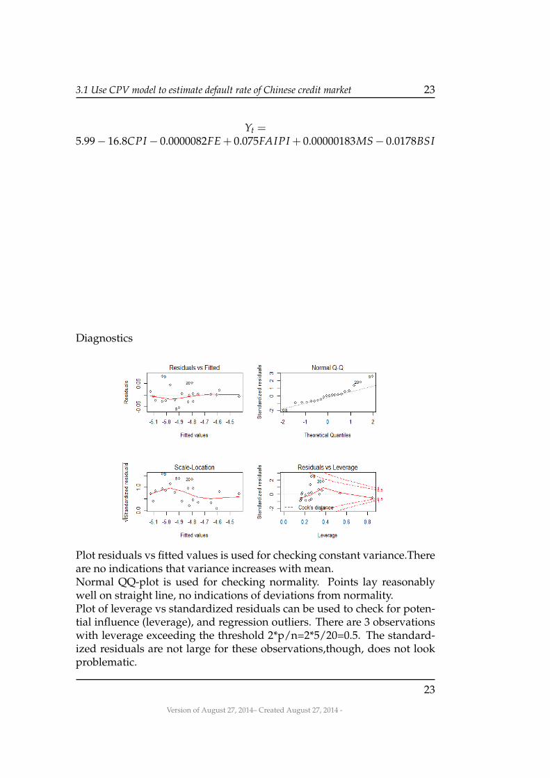
Yt =5.99− 16.8CPI− 0.0000082FE+ 0.075FAIPI + 0.00000183MS− 0.0178BSI

Diagnostics

Plot residuals vs fitted values is used for checking constant variance.Thereare no indications that variance increases with mean.Normal QQ-plot is used for checking normality. Points lay reasonablywell on straight line, no indications of deviations from normality.Plot of leverage vs standardized residuals can be used to check for poten-tial influence (leverage), and regression outliers. There are 3 observationswith leverage exceeding the threshold 2*p/n=2*5/20=0.5. The standard-ized residuals are not large for these observations,though, does not lookproblematic.


23


Table 3.8: comparing with real default rate and estimate default rate

Real Default Rate Estimate Default Rate0.0117 0.0112990.0103 0.0096890.0099 0.0094960.0095 0.0090850.0086 0.0082050.008 0.007668

0.0076 0.0072360.007 0.0070750.007 0.0061880.006 0.0057650.006 0.0058670.006 0.005652

0.0063 0.0062020.0065 0.0063730.007 0.006837

0.0072 0.0066120.0077 0.0076020.008 0.007881

0.0083 0.0078980.0086 0.007818

24



3.1.3 Calculating the default rate

0 5 10 15 20

0.00

00.

005

0.01

00.

015

0.02

00.

025

years

Def

ault

Rat

e

Trend about percentage of obligors in default

Default Raterealestimate


25


3.2 Use CPV model to estimate default rate ofDutch credit market

3.2.1 Macroeconomic factors and data

Comparing with the default rate of Chinese joint-equity commercial bank,I use GDP,GDP Growth,CPI,financial expenditure,unemployment rate,interestrate,value of exports,value of shares,exchange rate(dollar),and disposableincome to be the macroeconomic factors.I also use time series data on a quarter base over the years 2009-2013.AndI also choose the probability of the non-performing loan to be the defaultrate.The data of the non-performing loan is from the official website of Decentrale bank van Nederland[17],(http://www.dnb.nl/home/index.jsp),andthe data of all the macroeconomic factors is from the official website ofCentraal Bureau voor de Statistiek(http://www.cbs.nl/en-GB/menu/home/default.htm)[16]. Also as theCPV model,Pj,t =

11+e−Yj,t

,we can get Yj,t for every quarter.The results in

the table below.In the table all the data is adjusted by seasonal adjustment and CPI index.

Table 3.9: All of the required data

DR Y GDP CPI Growth UR FE IR VE ER VS DI0.0183 -3.98 136125 107.38 -0.020838 2.2 71107 3.74 45413.75 1.61 255493 573270.0244 -3.69 134183 107.39 -0.01427 2.5 74446 3.86 45853.63 1.65 291680 797230.0269 -3.59 135242 106.46 0.007892 2.6 71926 3.65 50718.59 1.67 351963 583090.0320 -3.41 135794 105.82 0.004082 2.9 77303 3.5 53809.24 1.7 383486 635130.0319 -3.41 136537 108.08 0.005472 3.3 73092 3.4 54976.71 1.68 400607 573620.0276 -3.56 136999 107.64 0.003384 3.1 79490 3.08 52906.83 1.71 382359 795650.0257 -3.64 137197 107.96 0.001445 2.7 71289 2.65 55473.88 1.76 399374 617420.0282 -3.54 138552 107.77 0.009876 2.6 77413 2.84 60210.07 1.67 423867 636110.0273 -3.57 139360 110.08 0.005832 2.9 72761 3.35 63797.67 1.68 438484 599040.0268 -3.59 139148 110.12 -0.00152 2.6 78241 3.44 66546.33 1.6 408607 825530.0272 -3.58 138698 111.15 -0.00323 2.6 71338 2.73 66371.52 1.53 356411 605550.0271 -3.58 137696 110.48 -0.00722 2.8 76375 2.43 62060.34 1.57 393273 646340.0294 -3.50 137315 113.26 -0.00277 3.2 73558 2.23 64217.45 1.67 411636 600750.0312 -3.43 137929 112.87 0.004471 3.1 79117 2.06 63202.37 1.68 400283 810770.0306 -3.45 136731 113.98 -0.00869 3.1 71953 1.78 61126.92 1.8 427506 615040.0310 -3.44 135919 114.2 -0.00594 3.3 77461 1.66 63279.58 1.62 438103 648120.0278 -3.55 135414 116.88 -0.00372 4 70224 1.74 65103.45 1.51 456433 597520.0300 -3.48 135191 116.44 -0.00165 4.1 79366 1.78 63306.37 1.51 459106 802320.0295 -3.49 135929 116.7 0.005459 4.1 72934 1.66 64655.91 1.57 492268 626610.0323 -3.40 136887 115.81 0.007048 4.7 77505 1.74 64989.57 1.69 507518 67544

3.2.2 Model building

In CPV model,Yj,t is an index value derived using a multi-factor regressionmodel that considers a number of macro economic factors, j representingthe industry and t the time period.

26


3.2 Use CPV model to estimate default rate of Dutch credit market 27

Yj,t = ws,0 + ∑Kk=1 ws,kXs,k,t + εs,t,

So In this case study

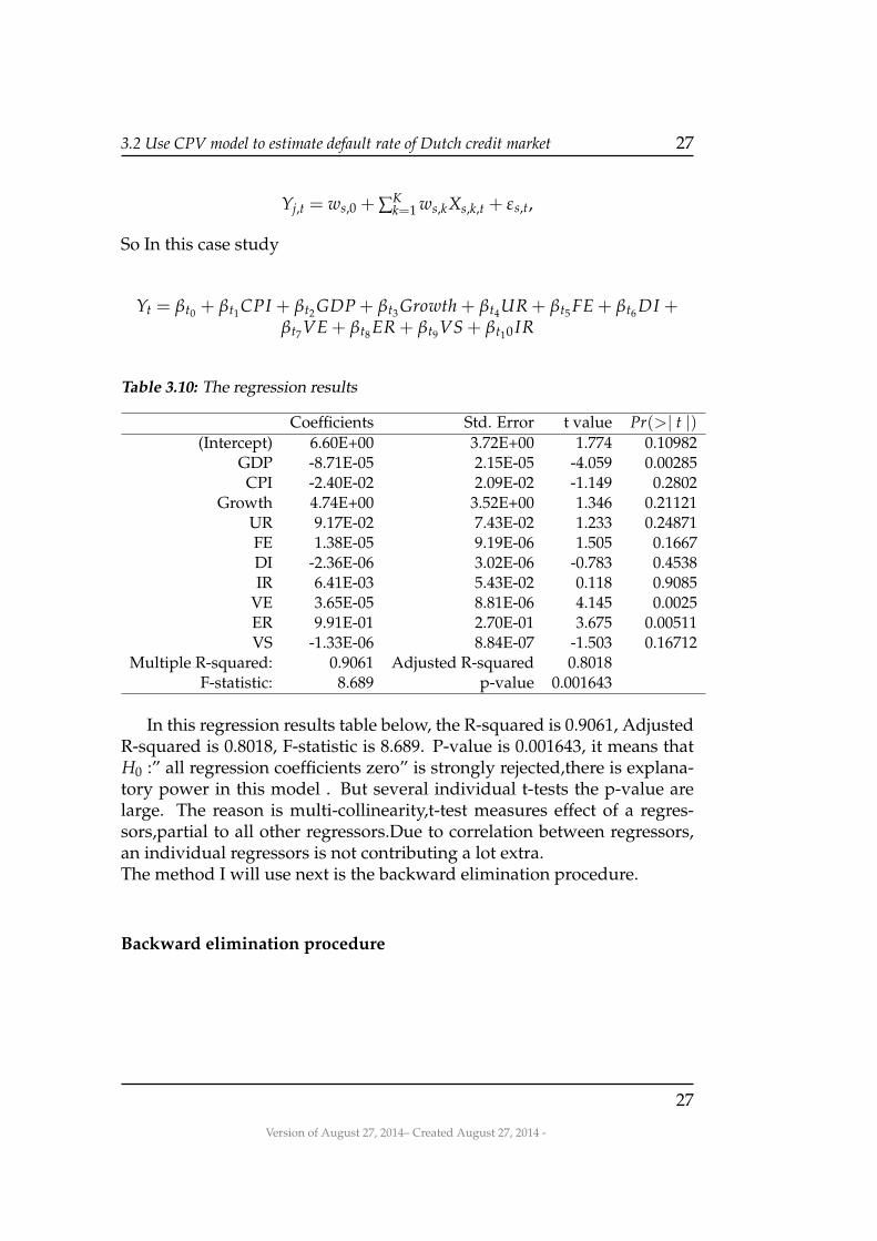
Yt = βt0 + βt1CPI + βt2 GDP + βt3 Growth + βt4UR + βt5 FE + βt6 DI +βt7VE + βt8 ER + βt9VS + βt10 IR

Table 3.10: The regression results

Coefficients Std. Error t value Pr(>| t |)(Intercept) 6.60E+00 3.72E+00 1.774 0.10982

GDP -8.71E-05 2.15E-05 -4.059 0.00285CPI -2.40E-02 2.09E-02 -1.149 0.2802

Growth 4.74E+00 3.52E+00 1.346 0.21121UR 9.17E-02 7.43E-02 1.233 0.24871FE 1.38E-05 9.19E-06 1.505 0.1667DI -2.36E-06 3.02E-06 -0.783 0.4538IR 6.41E-03 5.43E-02 0.118 0.9085

VE 3.65E-05 8.81E-06 4.145 0.0025ER 9.91E-01 2.70E-01 3.675 0.00511VS -1.33E-06 8.84E-07 -1.503 0.16712

Multiple R-squared: 0.9061 Adjusted R-squared 0.8018F-statistic: 8.689 p-value 0.001643

In this regression results table below, the R-squared is 0.9061, AdjustedR-squared is 0.8018, F-statistic is 8.689. P-value is 0.001643, it means thatH0 :” all regression coefficients zero” is strongly rejected,there is explana-tory power in this model . But several individual t-tests the p-value arelarge. The reason is multi-collinearity,t-test measures effect of a regres-sors,partial to all other regressors.Due to correlation between regressors,an individual regressors is not contributing a lot extra.The method I will use next is the backward elimination procedure.

Backward elimination procedure


27


Table 3.11: Backward elimination procedure table

Start AIC=-107.61 Df Sum of Sq RSS AICIR 1 0.000048 0.030711 -109.578DI 1 0.002088 0.032751 -108.291

none 1 0.030663 -107.609CPI 1 0.004497 0.03516 -106.871UR 1 0.005182 0.035845 -106.486

Growth 1 0.006173 0.036836 -105.94VS 1 0.007695 0.038358 -105.13FE 1 0.007712 0.038375 -105.122ER 1 0.046019 0.076682 -91.276

GDP 1 0.056131 0.086794 -88.799VE 1 0.058523 0.089186 -88.255


DI 1 0.002328 0.033038 -110.116none 0.01095 -130.2

Growth 1 0.006138 0.036848 -107.933UR 1 0.006204 0.036914 -107.898VS 1 0.007801 0.038512 -107.05

CPI 1 0.0095 0.04021 -106.187FE 1 0.009567 0.040278 -106.154ER 1 0.05324 0.083951 -91.465

GDP 1 0.057926 0.088637 -90.379VE 1 0.058523 0.089234 -90.245


none 0.033038 -110.116Growth 1 0.005289 0.038328 -109.146

VS 1 0.006363 0.039401 -108.594UR 1 0.007125 0.040163 -108.211FE 1 0.010228 0.043267 -106.722

CPI 1 0.013641 0.04668 -105.204ER 1 0.052847 0.085885 -93.01

GDP 1 0.058459 0.091497 -91.744VE 1 0.060749 0.093788 -91.249

28



The AIC is used for backward elimination. AIC = 2 log(likelihood) +2p with p the number of parameters in the model, smaller values point tobetter fitting models. Each variable is removed from the model in turn,and the resulting AIC’s are reported. For 8 regressors the AIC deterio-rates (becomes larger) by removal, so these variables are important. For2 regressors removal makes the AIC smaller (better), so these regressorsare candidates for removal. After we remove them the model is Yt = βt0 +βt1CPI + βt2 GDP+ βt3 Growth+ βt4UR+ βt5 FE+ βt6VE+ βt7 ER+ βt8VSThe regression results is in the table below

Table 3.12: regression results after removing IR and DI

Coefficients Std. Error t value Pr(>| t |)(Intercept) 7.38E+00 3.13E+00 2.361 0.037751

data1$GDP -8.69E-05 1.97E-05 -4.412 0.001043data1$CPI -2.94E-02 1.38E-02 -2.131 0.056467

data1$Growth 4.31E+00 3.25E+00 1.327 0.211386data1$UR 1.01E-01 6.54E-02 1.54 0.151774data1$FE 7.93E-06 4.30E-06 1.845 0.09205data1$VE 3.71E-05 8.25E-06 4.497 0.000905data1$ER 9.75E-01 2.32E-01 4.195 0.001499data1$VS -1.18E-06 8.09E-07 -1.455 0.173475

Multiple R-squared: 0.8989 Adjusted R-squared 0.8253F-statistic: 12.22 p-value 0.0001778


29


In this regression results table below, the R-squared is 0.8989, AdjustedR-squared is0.8253, F-statistic is 12.22. P-value is 0.0001778, it also meansH0 :” all regression coefficients zero” is strongly rejected,there is explana-tory power in this model . But for the individual t-tests:the p-values ofGDP Growth,and value of shares,are still big.We try to remove them and build a new model.

Yt = βt0 + βt1CPI + βt2 GDP + βt3UR + βt4 FE + βt5VE + βt6 ER The re-gression results is in the table below

Table 3.13: regression results after removing IR,DI,Growth and VS

Coefficients Std. Error t value Pr(>| t |))(Intercept) 7.60E+00 3.03E+00 2.51 0.026102

data1$GDP -8.23E-05 1.97E-05 -4.179 0.00108data1$CPI -3.68E-02 9.60E-03 -3.83 0.002084data1$UR 8.08E-02 3.95E-02 2.046 0.06155data1$FE 7.63E-06 4.42E-06 1.729 0.10741data1$VE 3.36E-05 5.88E-06 5.707 7.21E-05data1$ER 8.41E-01 1.96E-01 4.298 0.000867

In the table we can also see the p-values of all the factors are not toolarge. So the final model is

Yt = βt0 + βt1CPI + βt2 GDP+ βt3UR+ βt4 FE+ βt5VE+ βt6 ER Accord-ing to the table of The regression results of final model,we can get themodel of Yt

Yt = 7.6− 0.000083GDP− 0.0368CPI + 0.081UR + 0.00000763FE +0.0000336VE + 0.841ER

30



Table 3.14: comparing with real default rate and estimate default rate

real default rate estimate default rate0.0183 0.0188560.0244 0.0242610.0269 0.0271650.0320 0.0321120.0319 0.0285380.0276 0.0276260.0257 0.0277660.0282 0.0282410.0273 0.0273270.0268 0.0289270.0272 0.0257830.0271 0.0270860.0294 0.0297470.0312 0.0289630.0306 0.0299440.0310 0.0310630.0278 0.028550.0300 0.030030.0295 0.0293490.0323 0.033919


31


3.2.3 Calculating the default rate

0 5 10 15 20

0.00

00.

005

0.01

00.

015

0.02

00.

025

0.03

00.

035

years

Def

ault

Rat

e


Default Raterealestimate

In the table above we can see that the real default rate and estimate defaultrate are similar, so it shows that our model is meaningful.

32


Chapter 4Estimation Default Risk of BothChinese and Dutch CompaniesBased on KMV Model

4.1 Use KMV model to evaluate default risk forCNPC and Sinopec Group

1.Data Source My study sample are the financial data of the largest twopetrochemical company of China(CNPC and Sinopec Group) from the sec-ond quarter of 2012 to the third quarter of 2013. The related data are:(interestrate,daily stock closing price,the market value,short-term liabilities andlong-term liabilities).Daily stock closing price only take available opendays prices.The data is from the website of the Netease Finance.[18] (http ://quotes.money.163.com)

2.The Market value: The market value of the two companies are shownin the table below

3.Default Point Calculation According to the KMV model the DP = STD+0.5LTD,the STD is short-term liabilities,and LTD is long-term liabilities.TheDP of the 2 companies are shown in the table below.


33

34Estimation Default Risk of Both Chinese and Dutch Companies Based on KMV Model

Table 4.1: The market value of CNPC and Sinopec Group

CNPC Sinopec Group2012Q3 1.66915E+12 5.42626E+112012Q4 1.60692E+12 5.20053E+112013Q1 1.65451E+12 6.04269E+112013Q2 1.39279E+12 4.97734E+112013Q3 1.43488E+12 5.1755E+11

34


4.1 Use KMV model to evaluate default risk for CNPC and Sinopec Group 35

Table 4.2: The default point of CNPC and Sinopec Group(Million Yuan)

CNPC Sinopec Group2012Q3 772965 5465732012Q4 781410 5948902013Q1 835995 6149022013Q2 863635 5986052013Q3 903328 586453

4.Asset value and Asset Value Fluctuation Ration Calculation We usehistorical stock closing price data to calculate the stock fluctuation ratioσs, assuming the historical data fit the log-normal distribution, the dailylogarithmic profit ratio is

ui = ln( SiSi−1

)

Where Si is the relative daily stock closing price.So the stock fluctuationrationFluctuation ratio in daily stock returns is:

S =

√√√√ 1n− 1

n−1

∑1(ui − u)

Where u is the mean of ui .Number of trading days quarterly of the stock isN , relationship between the quarterly fluctuation ratio σs and daily fluc-tuation ratio S is

σs = S√

N

The stock fluctuation ratio σs of the two companies are shown in the tablebelow.

Table 4.3: The stock fluctuation ratio σs of CNPC and Sinopec Group

CNPC Sinopec Group2012Q3 0.070034545 0.1150958492012Q4 0.069165841 0.0978944542013Q1 0.069165841 0.1159357522013Q2 0.068029746 0.3174940852013Q3 0.070759383 0.115512544


35


According to the formula above we can estimate the asset value and it’svolatility. I use matlab 2012b to solve the nonlinear equations, the code are

1 function F=KMVfun(EtoD,r,T,EquityTheta,x)2 d1=(log(x(1)∗EtoD)+(r+0.5∗x(2)ˆ2∗T))/x(2);3 d2=d1−x(2);4 F=[x(1)∗normcdf(d1)−exp(−r)∗normcdf(d2)/EtoD−1;normcdf(d1)∗x(1)∗x(2)5 −EquityTheta];6 end7 function [Va,AssetTheta]=KMVOptSearch(E,D,r,T,EquityTheta)8 EtoD=E/D;9 x0=[1,1];

10 VaThetax=fsolve(@(x)KMVfun(EtoD,r,T,EquityTheta,x),x0);11 Va=VaThetax(1)∗E;12 AssetTheta=VaThetax(2);13 end

The relative asset value and it’s volatility are shown in the table below.

Table 4.4: asset value of CNPC and Sinopec Group(Million Yuan)

CNPC Sinopec Group2012Q3 2420000 10700002012Q4 2370000 11000002013Q1 2470000 12000002013Q2 2230000 10800002013Q3 2310000 1090000

Table 4.5: The asset volatility of CNPC and Sinopec Group


5.Find the default distance(DD) At last,according to the formula above,wecan find DD of the three firms, I also use matlab 2012b to do the calcula-tion. The matlab code are:

36



1 function F=DDfun(Va,AssetTheta,D)2 F=[(Va−D)/(Va∗AssetTheta)];

The relative results are shown in the table below.

Table 4.6: The default distance of CNPC and Sinopec Group


We calculate the asset value, asset volatility and default distance in thesecond quarter of 2012 of CNPC as an example, the Matlab code are:

1 >> r=0.03;2 T=1;3 E=1.66915E+12;4 D=7.72965E+11;5 EquityTheta=0.070034545;6 [Va,AssetTheta]=KMVOptSearch(E,D,r,T,EquityTheta)7 [DD]=DDfun(Va,AssetTheta,D)8

9 Equation solved.10

11 fsolve completed because the vector of function values is near zero12 as measured by the default value of the function tolerance, and13 the problem appears regular as measured by the gradient.14

15 <stopping criteria details>16

17

18 Va =19

20 2.4193e+1221

22

23 AssetTheta =24

25 0.048326


37


27

28 DD =29

30 14.0832

The results of the code above shows that the asset value, asset volatil-ity and default distance of CNPC in the second quarter of 2012. We canchange the Initialize variables and repeat the procedure to calculate theasset value, asset volatility and default distance for other time period andcompanies.

6.Comparing the default distance with the total assets turnover The To-tal assets turnover of the two companies are shown in the table below.

Table 4.7: The Total assets turnover of CNPC and Sinopec Group


Comparison of Total assets turnover and default distance of CNPC

Comparison of Total assets turnover and default distance of SinopecGroup.

38




39


4.2 Use KMV model to evaluate default risk forRoyal Dutch Shell and Royal Philips

1.Data source My study sample are the financial data of the largest twoDutch companies,(Royal Dutch Shell and Royal Philips) from the secondquarter of 2012 to the third quarter of 2013. The related data are:( interestrate,daily stock closing price,the market value,short-term liabilities andlong-term liabilities),the data is from the official webset of the two compa-nies and YAHOO Fiance.(http://finance.yahoo.com/)[19]

2.The Market value: The market value of the two companies are shownin the table below

Table 4.8: Market Value of Royal Dutch Shell and Royal Philips

Royal Dutch Shell Royal Philips2012Q3 2.26E+11 2.18E+102012Q4 2.24E+11 2.43E+102013Q1 2.11E+11 2.70E+102013Q2 2.10E+11 2.46E+102013Q3 2.19E+11 2.95E+10

3.Default Point Calculation According to the KMV model the DP = STD+0.5LTD,the STD is short-term liabilities,and LTD is long-term liabilities.TheDP of the 2 companies are shown in the table below.

Table 4.9: Default Point of Royal Dutch Shell and Royal Philips

Royal Dutch Shell Royal Philips2012Q3 1.39698E+11 133845000002012Q4 1.33689E+11 139255000002013Q1 1.37688E+11 130810000002013Q2 1.29279E+11 131195000002013Q3 1.33995E+11 12752500000

4.Asset value and Asset Value Fluctuation Ration Calculation We use his-torical stock closing price data to calculate the stock fluctuation ratio σs,assuming the historical data fit the log-normal distribution, the daily log-

40


4.2 Use KMV model to evaluate default risk for Royal Dutch Shell and Royal Philips 41

arithmic profit ratio is

ui = ln( SiSi−1

)

Where Si is the relative daily stock closing price.Fluctuation ratio in daily stock returns is:

S =√

1n−1 ∑n−1

1 (ui − u)

Where u is the mean of ui .Number of trading days quarterly of the stock isN , relationship between the quarterly fluctuation ratio σs and daily fluc-tuation ratio S is

σs = S√

N

The stock fluctuation ratio σs of the two companies are shown in the tablebelow.

Table 4.10: The volatility of equity of Royal Dutch Shell and Royal Philips

Royal Dutch Shell Royal Philips2012Q3 0.062748481 0.098514472012Q4 0.073478442 0.1021245532013Q1 0.056810285 0.125470932013Q2 0.069778976 0.0888400432013Q3 0.077046101 0.09262708

According to the formula above we can find the asset value and it’svolatility. I use matlab 2012b to solve the nonlinear equations, the relativeasset value and it’s volatility are shown in the table below.

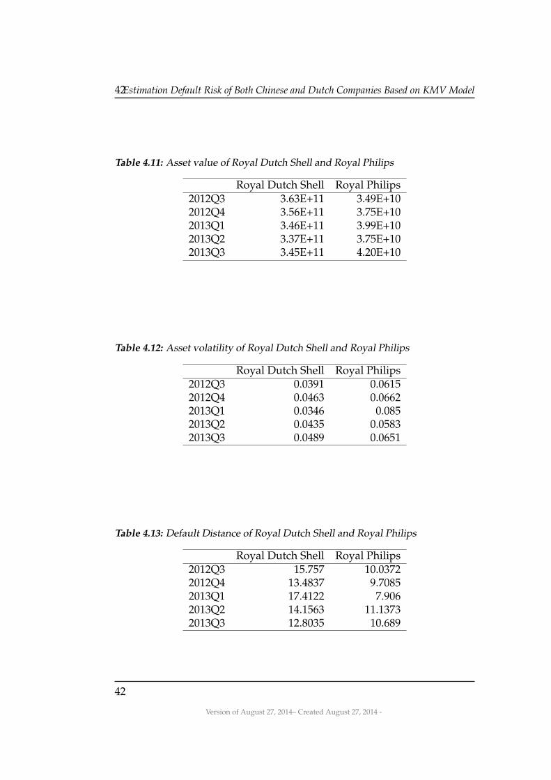
5.Find the default distance(DD) At last,according to the formula above,wecan find DD of the three firms, I also use matlab 2012b to do the calcula-tion. The relative results are shown in the table below.


41


Table 4.11: Asset value of Royal Dutch Shell and Royal Philips

Royal Dutch Shell Royal Philips2012Q3 3.63E+11 3.49E+102012Q4 3.56E+11 3.75E+102013Q1 3.46E+11 3.99E+102013Q2 3.37E+11 3.75E+102013Q3 3.45E+11 4.20E+10

Table 4.12: Asset volatility of Royal Dutch Shell and Royal Philips


Table 4.13: Default Distance of Royal Dutch Shell and Royal Philips


42


Chapter 5Prediction of default risk of aportfolio

The previous chapters discuss various ways to model and estimate thedefault risk of a single company. Most investors, in particular banks andinsurance companies, lend money to many companies and individuals. Itis important for them to understand the risk profile of their entire portfo-lio of loans. This risk profile is determined by the risks of the individualobligors and their correlations. In this chapter we study the influence ofcorrelations between obligors on the default risk of a portfolio.

5.1 Two models

Consider a bank with a portfolio of loans. Let N be the number of obligorsand let Li be the amount of the loan of obligor i, i = 1, · · · , N.For the bank it is important to understand the average expected loss dueto defaults as well as the risk of big losses. For instance,1. How much do we expect to loose next year.2. What is the probability that we will loose more than 10 percent of theportfolio next year?In order to answer these questions the bank will use models and historicdata to fit the parameters in the model. The historic data contains for eachobligor for many past months whether he was in default or not. We willfocus on two models: one without correlations and one with correlations.We will investigate how these models can be used for risk predictions andhow the choice of models affects the predicted risk.


43

44 Prediction of default risk of a portfolio

5.1.1 The Uniform Bernoulli Model

If we assume1.All loans are the same amount, which we scale to be 1.2.All obligors have same default probability p per year.3.All obligors are independent,the model becomes a Uniform Bernoulli Model.

Li ∼ B(1; p), i.e., Li =

{1 with probability p,0 with probability 1− p,

Li, i = 1, ..., N independent.

Note that the expected number of defaults is p ∗ NAccording to the Maximum Likelihood Estimator we can estimate p bymeans of the historic data,

pi =nmber of defaults in year i

Ni = 1, ..., T

p = 1/T( p1 + .... + pT)

where T is the number of years in historic data.

5.1.2 Factor Model

The assumption from that all obligors are independent is not very realis-tic. It may be expected that the financial strength of obligor depends oncertain factors in the economy. If a group of obligors depends of the samefactor, they will be correlated through that factor. The factor model cap-tures this feature.Assume that the set of obligors is divided into two groups:1, . . . , N = I1 ∪ I2 ∪ . . .∪ Ik, where Ii ∪ Ik =∅. We view the setIi as all oblig-ors of factor type i. We also assume all obligors of type i have the defaultprobability pi, and all obligors are independent.Then we can use Factor model to estimate the default probability.

44


5.1 Two models 45

In each year obligor i has a log asset value:

ri = RiΦ + εi

whereRi ∈ [−1,1],Φ ∼ N(0,1), εi ∼ N(0,1− (Ri)

2), Φ and εi independent.Then

RiΦ ∼ N(0, R2i )

SoEri = RiEΦ + Eεi = 0

And,

V = E(ri)2 = E(RiΦ + εi)

2

= E(RiΦ)2 + 2ERiΦεi + E(εi)2

= R2i + (1− R2

i ) = 1.

Sori ∼ N(0,1)

Obligor i is default if ri < −c, this happen with probability

P(ri < −c) = F(−c) = p

where

F(x) =1√2π

∫ x

−∞exp(−y2

2)dy

If all Ri = 0, then all of the obligors are independent.If all Ri = 1, then all of the obligors are in default or not.

Estimate the Ri and −c from the historic data

Now we need to estimate the Riand− c from the historic data. The bankdoes not observe ri, but only ri < −c or not.For estimate -c,we have

P(ri < −c) = p


45


And we can estimate p by using

p =Number of default obligors

Total number of obligors

So -c is the ”quantile” of the normal distribution corresponding to proba-bility p.

Next we consider estimating the coefficients Ri. We will use the esti-mator V for E[number of defaults2] given by V = (Number of default)2.We have

P (obligor 1 and obligor 2 both default)= P(r1 < −c and r2 < −c)= E[P(R1Φ + ε1 < −c and R2Φ + ε2 < −c|Φ = S)],

P(ε1 < −c− R1S and ε2 < −c− R2S)= P(ε1 < −c− R1S)P(ε2 < −c− R2S)

= P(ε1√

1− R21

<−c− R1S√

1− R21

)P(ε2√

1− R22

<−c− R2S√

1− R22

)

= F(−c− R1S√

1− R21

)F(−c− R2S√

1− R22

).

As P(r1 < −c and r2 < −c)= EP[R1Φ + ε1 < −c and R2Φ + ε2 < −c | Φ = S]

= E[F(−c− R1Φ√

1− R21

)F(−c− R2Φ√

1− R22

)].

Let us make one more assumption to simplify the model. We will assumethat all obligors have the same coefficient of dependence of Φ. In otherwords, all the Ri are the same, so Ri = R

46


5.1 Two models 47

Then,

E F(−c− R1Φ√

1− R21

)F(−c− R2Φ√

1− R22

)

= EF(−c− RΦ√

1− R2)F(−c− RΦ√

1− R2)

=∫

RF(−c− RS√

1− R2)F(−c− RS√

1− R2)

1√2π

exp(−S2

2)dS

Consider one year situation:

Li =

{1 ri < −c,obligor i in default0 ri ≥ −c,obligor i not in default

We have

E[(L1 + · · ·+ LN)2] = E

N

∑i=1

N

∑j=1

LiLj =N

∑i=1

N

∑j=1

ELiLj

For i 6= j we have

ELiLj = E1ri<−c1rj<−c = E1ri<−c andrj<−c

And

P (ri < −c andrj < −c)

=∫

RF(−c− R1S√

1− R21

)2 1√2π

exp(−S2

2)ds

For i=j we haveELiLj = EL2

i = p

HenceE[(L1 + · · ·+ LN)

2] = N(N − 1)Hc(R) + Np

Where,

Hc(R) =∫

RF(−c− R1S√

1− R21

)2 1√2π

exp(−S2

2)ds

SinceE[(L1 + · · ·+ LN)2] is estimated byV, and c by c, we obtain the fol-

lowing estimate for R:So

R = H−1C

(V − Np

N(N − 1))


47


Computing more than 10 percent of the portfolio defaults next year

The probability that exactly k of N obligors in default is

P (exactly k of N obligors in default)= EP(exactly k of N obligors in default | Φ = S)

Given thatΦ = S,

Obligor 1 is in default precisely when

r1 < −c

SoRS + ε1 < −c,

which is equivalent to

ε1√1− R2

<−c− RS√

1− R2

Hence,

P(obligor 1 in default | Φ = S) = F(−c− RS√

1− R2)

Since,ε1√

1− R2for i=1,...N are independent N(0,1) variable we find

P (exactly k of N obligors in default | Φ = S)

=

(Nk

)F(−c− RS√

1− R2)k(1− F(

−c− RS√1− R2

))N−k

Thus, taking expectation over the values S,

P (exactly k of N obligors in default)

=

(Nk

)∫R

F(−c− RS√

1− R2)k(1− F(

−c− RS√1− R2

))N−k 1√2π

exp( − S2

2)dS

So,

P (more than 10 percent of obligors in default)

= 1−P(less thanN10− 1 obligors in default)

= 1−N10−1

∑k=0

(Nk

)∫R

F(−c− RS√

1− R2)k(1− F(

−c− RS√1− R2

))N−k 1√2π

exp( − S2

2)dS

48


5.2 Computer simulation 49

5.2 Computer simulation

According to the models we want to use computer to test1. How dose the default change if we change the model.2.In the factor model, how does the the number of default obligors change,if we change the sensitivity coefficient R.

5.2.1 Simulation of the Uniform Bernoulli Model

The simulation procedure of the Uniform Bernoulli Model are:1. Data ProductionWe take the number of obligors N = 1000, time duration T = 20(years),default probability for each obligor is p = 0.05. Because this is UniformBernoulli Model, we assume each obligor has the same default probabil-ity. So for each year, we generate N independent Bernoulli variables withparameter p.2. Estimate the next time period default probability.We use maximum likelihood estimator to estimate the default probabilitypfor each obligor. Using p to estimate the probability that more than q% ofthe obligors will in default for q running from 0.1% to 10% for the nexttime period.

R code for Uniform Bernoulli Model Simulation

1 sam1<−replicate(20,sample(c(0,1),size=1000,replace = TRUE,prob=c(0.95,0.05)))2

3

4

5 phat1<−length(sam1[sam1==1])/length(sam1)6

7 p1<−1−pbinom(0.05∗1000,1000,phat1)8

9 prob<−c()10 for(i in 1:100){11

12 prob[i]<−1−pbinom(i,N,phat1)13 }14 xrange <− range(0,0.1)15


49


16 yrange <− range(0,1)17

18 percentage<−c(seq(0,0.1,length=100))19

20 probabilty<−prob21

22 plot(yrange˜xrange, type="n", xlab="percentage of obligors in default",23 ylab="probability" )24

25 lines(probabilty˜percentage, lwd=1.5,type="o",26 col="blue")

0.00 0.02 0.04 0.06 0.08 0.10

0.0

0.2

0.4

0.6

0.8

1.0

percentage of obligors in default

prob

abili

ty

The picture shows that the probability that more than q% of the obligor isin default equals 1 if q = o, as expected, and goes down to 0 as q goes to100%. The steapest decay is around 0.05(5%), which is the default proba-bility for each obligor.

50



5.2.2 Simulation of the Factor Model

The simulation procedure of the Factor Model are:1. Data ProductionWe take the number of obligors N = 1000, time duration T = 20(years), andwe let the sensitivity coefficient R vary in the range(0.2,0.4,0.6,0.8). If thelog of obligor’s asset value ri < −c, means obligori in default. We chooseagain the default probability p equal to 0.05. So −c = Q(0.05), where Qis the quantile function of standard normal distribution, Φ is the compos-ite factor of obligors, and Φ ∼ N(0,1). We generate 20 N(0,1) randomvariable for Φ each corresponding to one of the 20 years. Moreover wegenerate 20×N N(0, (1− R2)) independent random variables for εi. Withthese values we compute for each of the 20 years the values

ri = RΦ + εi, 1 = 1, ...N.

For each of the 20 years we compute Li,i = 1, ...N, by Li = 1 if ri < −c andLi = 0 otherwise.2. Estimate the next time period default probability.We use maximum likelihood estimator to estimate the default probabilityp.We estimate V, c, and R by means of the formulas in section 5.12, averagedover the 20 years. for each obligor. Computing the probability that morethan (0%,10%) of the obligors will in default in the next time period. Wedo the whole procedure for each of the sensitivity coefficients R.

R code for Factor Model Simulation

1 N<−10002

3 R<−0.24

5 c<−−qnorm(0.3)6

7 theta<−rnorm(20,mean=0,sd=1)8

9 epsilon<−replicate(20,rnorm(1000,0,1−Rˆ2))10

11 r<−epsilon12 for(i in 1:20){13 r[,i]<− R∗theta[i]+epsilon[,i]14 }


51


15

16 sam2<− apply(r,2,function(x) as.numeric(x<=−c))17

18

19

20 phat2<−length(sam2[sam2==1])/length(sam2)21

22 chat<−−qnorm(phat2)23

24 Vhat<−1/20∗(sum(sam2[,1])ˆ2+sum(sam2[,2])ˆ2+sum(sam2[,3])ˆ225 +sum(sam2[,4])ˆ2+sum(sam2[,5])ˆ226 +sum(sam2[,6])ˆ2+sum(sam2[,7])ˆ2+sum(sam2[,8])ˆ227 +sum(sam2[,9])ˆ2+sum(sam2[,10])ˆ228 +sum(sam2[,11])ˆ2+sum(sam2[,12])ˆ229 +sum(sam2[,13])ˆ2+sum(sam2[,14])ˆ230 +sum(sam2[,15])ˆ2+sum(sam2[,16])ˆ231 +sum(sam2[,17])ˆ2+sum(sam2[,18])ˆ232 +sum(sam2[,19])ˆ2+sum(sam2[,20])ˆ233 )34

35

36

37 a<−NULL38

39

40

41 g<−function(a){42 integrate(function(x){43 (pnorm((−chat−a∗x)/sqrt(1−aˆ2)))ˆ2∗(1/sqrt(2∗pi))∗exp((−xˆ2)/2)44 },−Inf,Inf)45

46 }47

48

49

50 h<−function(a){51 g(a)$value−(Vhat−N∗phat2)/(N∗(N−1))}52

53 Rhat<−uniroot(h,c(0,0.99999))54

55

56 prob0.2<−c()57

52



58 for(i in 1:1000){59

60 e<−function(s){61

62 pbinom(i,N,pnorm((−chat−Rhat$root∗s)/sqrt(1−Rhat$rootˆ2)))∗dnorm(s)63 }64

65 prob0.2[i]<1−integrate(e,−Inf,Inf)$value66 }67

68

69 #Change R from 0.2 to 0.4,0.6,0.8, run pervious code again70 #we can get the corresponding default probability (prob0.4,prob0.6,prob0.8).71

72

73

74 Default<−data.frame(R=rep(c(0.2,0.4,0.6,0.8),each=100),75 Probabilty=c(prob0.2,prob0.4,prob0.6,prob0.8),76 percentage=c(seq(0,0.1,length=100),seq(0,0.1,length=100),77 seq(0,0.1,length=100),seq(0,0.1,length=100)))78

79

80

81

82 # Create Line Chart83

84 # convert factor to numeric for convenience85 Default$R <− as.numeric(Default$R)86 nR <− max(Default$R)87

88 # get the range for the x and y axis89 xrange <− range(0,0.1)90 yrange <− range(0,1)91

92 # set up the plot93 plot(yrange˜xrange, type="n", xlab="percentage of obligors in default",94 ylab="probability" )95 colors <− rainbow(4)96 linetype <− c(1:4)97 plotchar <− seq(18,18+4,1)98

99 # add lines100 for (i in 1:4) {


53


101 R <− subset(Default, R==as.numeric(levels(as.factor(Default$R)))[i])102 lines(R$Probabilty˜R$percentage, lwd=1.5,type="o",103 lty=linetype[i], col=colors[i], pch=plotchar[i])104 }105

106 # add a title and subtitle107 title("Trend about percentage of obligors in default ")108

109 # add a legend110 legend("bottomleft",xrange[1], c(0.2,0.4,0.6,0.8), cex=0.8, col=colors,111 pch=plotchar, lty=linetype, title="R")

0.0 0.2 0.4 0.6 0.8 1.0

0.0

0.2

0.4

0.6

0.8

1.0


prob

abili

ty


R0.20.40.60.8

With the default probability 0.3. We see from the picture that the curves

54



decrease from 1 to 0, as expected. The curves become less and less step ifthe factor R increases. Since R is the coefficient describing the dependenceof the joint factor Φ, it is expected that the default correlation get higher ifR increases. We see in the picture that this indeed happens. In therms ofcredit risk management, this means that the probability of a large loss getsconsiderably higher for higher values of R, where the default probabilityis still the same value.

0.00 0.02 0.04 0.06 0.08 0.10

0.0

0.2

0.4

0.6

0.8

1.0


prob

abili

ty


R0.20.40.60.8

Lower default probability(0.05): More or less the same situation, butthe decay of the curve now take place for lower percentage. This is asexpected, since for a lower default rate the probability that more than 10%of the obligors are in default will be much lower.


55

References

[1] Anthony, S., Marcia, C. (2010).Financial Institu-tions Management: A Risk Management Approach,McGraw-Hill/Irwin; 7 edition.

[2] Bluhm, C., Overbeck, L., Wagner, C. (2002). An intro-duction to credit risk modeling. CRC Press.

[3] Chan-juan,C and Hai-bo Z. ”Toward the Application ofCPV Model in the Calculation of Loan Default Proba-bility [J].” Modern Economic Science 5 (2009): 006.

[4] Du, Y., Suo, W. (2003). Assessing Credit Qualityfrom Equity Markets: Is Structural Model a Better Ap-proach?. Available at SSRN 470701.

[5] Faraway (2006). Extending the linear model with R.Generalized linear, mixed effects and nonparametric re-gression models. Chapman Hall/CRC

[6] Gordy, M. B. (2003). A risk-factor model foundation forratings-based bank capital rules. Journal of financial in-termediation, 12(3), 199-232.

[7] Gelman, A., Hill, J. (2006). Data analysis using regres-sion and multilevel/hierarchical models. CambridgeUniversity Press.

[8] Jiang, L. (2005). Mathematical modeling and methodsof option pricing. Singapore: World Scientific.

[9] Junxian L., Maureen Olsson L(2009). ”CREDIT RISKMANAGEMENT OF THE CHINESE BANKS BASEDON THE KMV MODEL ” Master’s Degree Thesis.


57

58 References

[10] Korablev, I., Dwyer, D. (2007). Power and level vali-dation of Moody’s KMV EDF credit measures in NorthAmerica, Europe, and Asia, Technical Paper, Moody’sKMV Company. Page 7.

[11] Kupiec, P. H. (2008). A generalized single common fac-tor model of portfolio credit risk. The Journal of Deriva-tives, 15(3), 25-40.

[12] Peter, C., Ahmet, K. (2003). MODELING DEFAULTRISK . Technical Paper, Moody’s KMV Company.

[13] Thorp, J. (2003). Change of seasonal adjustment methodto X-12-ARIMA. Monetary and Financial Statistics, 4-8.

[14] Website of National Bureau Of Statistics OfChina,(http://www.stats.gov.cn/).

[15] Website of China Banking Regulatory Commis-sion,(http://www.cbrc.gov.cn/index.html).

[16] Website of Centraal Bureau voorde Statistiek,(http://www.cbs.nl/en-GB/menu/home/default.htm).

[17] Website of De centrale bank van Neder-land,(http://www.dnb.nl/home/index.jsp).

[18] Website of the Netease Fi-nance,(http://quotes.money.163.com).

[19] Website of YAHOO Fi-ance,(http://finance.yahoo.com/).

[20] Xiaohong,C., Xiaoding, W, and Desheng, Wu. ”Creditrisk measurement and early warning of SMEs: An em-pirical study of listed SMEs in China.” Decision Sup-port Systems 49, no. 3 (2010): 301-310.

58


Documents

Mathematical Models And Statistical Analysis of Credit ... · Mathematical Models And Statistical Analysis of Credit Risk Management Tianfeng Hou Mathematical Institute, Universiteit