Embed Size (px)
Citation preview

HAL Id: tel-01867754https://tel.archives-ouvertes.fr/tel-01867754
Submitted on 4 Sep 2018
HAL is a multi-disciplinary open accessarchive for the deposit and dissemination of sci-entific research documents, whether they are pub-lished or not. The documents may come fromteaching and research institutions in France orabroad, or from public or private research centers.
L’archive ouverte pluridisciplinaire HAL, estdestinée au dépôt et à la diffusion de documentsscientifiques de niveau recherche, publiés ou non,émanant des établissements d’enseignement et derecherche français ou étrangers, des laboratoirespublics ou privés.
Mathematical modelling of the chitosan fiber formationby wet-spinning
Alexandru Alin Enache
To cite this version:Alexandru Alin Enache. Mathematical modelling of the chitosan fiber formation by wet-spinning.Chemical engineering. Université de Lyon; Universitatea politehnica (Bucarest), 2018. English.�NNT : 2018LYSE1100�. �tel-01867754�

N°d’ordre NNT : 2018LYSE1100
THESE de DOCTORAT DE L’UNIVERSITE DE LYON opérée au sein de
l’Université Claude Bernard Lyon 1 en cotutelle avec L’Université « Politehnica » De Bucarest,
Roumanie
Ecole Doctorale N° 34 Ecole doctorale Matériaux de Lyon
Spécialité de doctorat : GÉNIE CHIMIQUE
Soutenue publiquement le 21/06/2018, par : ALEXANDRU ALIN ENACHE
MATHEMATICAL MODELLING OF THE
CHITOSAN FIBER FORMATION BY WET-SPINNING
MODELISATION DU PROCEDE D’ELABORATION DE FIBRES DE
CHITOSANE Devant le jury composé de :
M. Dănuț- Ionel VĂIREANU Professeur, Université Politehnica de Bucarest President
M. Jacques FAGES Professeur, École Nationale Supérieure des Mines d’Albi-Carmaux (IMT Mines Albi)
Rapporteur
M. Teodor TODINCĂ Professeur, Université Politehnica de Timișoara
Rapporteur
Mme. Annelise FAIVRE Professeure, Université de Montpellier Examinatrice Mme. Sanda VELEA Directeur de recherche, ICECHIM Bucarest Examinatrice M. Laurent DAVID Professeur, Université Claude-Bernard Lyon 1 Examinateur
M. Jean-Pierre PUAUX Professeur, Université Claude-Bernard Lyon 1 Co-directeur de thèse
M. Grigore BOZGA Professeur, Université Politehnica de Bucarest Co-directeur de thèse

Mathematical Modelling of the Chitosan Fiber Formation by Wet-Spinning
2
UNIVERSITE CLAUDE BERNARD - LYON 1 Président de l’Université
Président du Conseil Académique
Vice-président du Conseil d’Administration
Vice-président du Conseil Formation et Vie Universitaire
Vice-président de la Commission Recherche
Directrice Générale des Services
M. le Professeur Frédéric FLEURY
M. le Professeur Hamda BEN HADID
M. le Professeur Didier REVEL
M. le Professeur Philippe CHEVALIER
M. Fabrice VALLÉE
Mme Dominique MARCHAND
COMPOSANTES SANTE Faculté de Médecine Lyon Est – Claude Bernard Directeur : M. le Professeur G.RODE
Faculté de Médecine et de Maïeutique Lyon Sud – Charles Mérieux
Directeur : Mme la Professeure C. BURILLON
Faculté d’Odontologie Directeur : M. le Professeur D. BOURGEOIS
Institut des Sciences Pharmaceutiques et Biologiques
Directeur : Mme la Professeure C. VINCIGUERRA
Institut des Sciences et Techniques de la Réadaptation
Directeur : M. X. PERROT
Département de formation et Centre de Recherche en Biologie Humaine
Directeur : Mme la Professeure A-M. SCHOTT
COMPOSANTES ET DEPARTEMENTS DE SCIENCES ET TECHNOLOGIE
Faculté des Sciences et Technologies
Département Biologie
Département Chimie Biochimie
Département GEP
Département Informatique
Département Mathématiques
Département Mécanique
Département Physique
UFR Sciences et Techniques des Activités Physiques et Sportives
Observatoire des Sciences de l’Univers de Lyon
Polytech Lyon
Ecole Supérieure de Chimie Physique Electronique
Institut Universitaire de Technologie de Lyon 1
Ecole Supérieure du Professorat et de l’Education
Institut de Science Financière et d'Assurances
Directeur : M. F. DE MARCHI
Directeur : M. le Professeur F. THEVENARD
Directeur : Mme C. FELIX
Directeur : M. Hassan HAMMOURI
Directeur : M. le Professeur S. AKKOUCHE
Directeur : M. le Professeur G. TOMANOV
Directeur : M. le Professeur H. BEN HADID
Directeur : M. le Professeur J-C PLENET
Directeur : M. Y.VANPOULLE
Directeur : M. B. GUIDERDONI
Directeur : M. le Professeur E.PERRIN
Directeur : M. G. PIGNAULT
Directeur : M. le Professeur C. VITON
Directeur : M. le Professeur A. MOUGNIOTTE
Directeur : M. N. LEBOISNE

Alin Alexandru ENACHE
3
ACKNOWLEDGEMENTS
This work was performed in the frame of a cooperation between the Department of Chemical
and Biochemical Engineering, University Politehnica of Bucharest, Romania and the
laboratory of Ingénierie des Matériaux Polymères (IMP), Univ Lyon, Université Lyon 1,
France. Firstly, I would like to thank Prof. Phillipe Cassagnau, the laboratory director, to
give me this opportunity to execute a part to my doctoral research in Lyon.
My greatest and sincerest gratitude goes to my Romanian supervisor Prof. Grigore BOZGA
who expertly guided me through my Ph.D. study. His constant support, patience, transfer of
knowledge and trust made this thesis possible.
My sincere thanks to my French supervisor Prof. Jean-Pierre PUAUX who made possible
my two stages in France and gave me all the advices regarding the research study. Thank
you for gave me the possibility to take contact with French culture.
My honest thanks go to Prof. Laurent DAVID for his numerous valuable advices regarding
the orientation and development of my research. Thanks a lot for his encouragements. I
thank you for your travel in Romania in order to present me the subject of my Ph.D. thesis.
I would like to thank Prof. Teodor TODINCĂ (University of Politehnica Timisoara,
Romania) and Prof. Jacques FAGES (École Nationale Supérieure des Mines d’Albi-
Carmaux (IMT Mines Albi)) kindly accepted to examine this work as reporters and members
of the jury. I warmly thank them for their helpful advices and observations.
I am eager to express my gratitude to members of the jury that they accepted to judge this
work: Prof. Laurent DAVID (Universite Claude Bernard, Lyon 1), Prof. Annelise FAIVRE
(Université de Montpellier II) and Chercheure Sanda VELEA (Institut National de
Recherche et Développement en Chimie et Pétrochimie –ICECHIM Bucuresti).
I would like to thank Prof. Dănuț- Ionel VĂIREANU, for his kindly acceptance to be the
president of the jury and for his advices regarding the experimental studies.
I would thank to conf. Gheorghe Bumbac for his constant support, patience, transfer of
knowledge.

Mathematical Modelling of the Chitosan Fiber Formation by Wet-Spinning
4
I would thank to Ionut BANU who gave me all the information needed before my travel in
France (he was the first at IMP from our department). Also, I would thank you to Prof. Vasile
LAVRIC, the Romanian doctoral school director, for all advices. Many thanks to Prof.
Tanase DOBRE who sponsored me to participate to RICCCE conference.
I thank all the Permanent staff of the Laboratory of Polymers Materials Engineering Lyon 1
for these beautiful moments spent in your company, especially to Agnès Crépet for her
expertise and assistance in molar mass determination by size exclusion chromatography
(SEC) measurements, Thierry Tamet, Flavien Melis, Ali Adan who assisted me during the
spinning study and for morning coffees, Olivier Gain, Pierre Alcouffe for his kind assistance
in microscopy, Florian Doucet and Laurent Cavetier who gave me all the mechanical and
electrical tools. Thanks to Sabine Sainte-Marie for the good times spent together and for the
wine bottles.
I am also thankful to the fellow graduate students, past and present, and the friends who
supported me and made my life better during my doctoral stage in France. My firstly special
‘thank you’ goes to my Tunisian brother, Imed, who shared with me the microscope and his
apartment for two weeks during my second stage in France. Also, I would thank to Julie and
Jihane because they integrated me in the France laboratory life. A special thank goes to
Nicolas who initiated me in the chitosan purification and hydrogel preparation, it was a
pleasure to work with him. Other fellows, Alice Galais who used to help me out in NMR
spectra data analysis; Mélanie who shared the spinning plant. Many thanks Perrine who was
the first person from the laboratory I told that I will have a baby. I also grateful to IMP team
members who have always been willing to help me in whatever way possible, have been a
joy to work with: Kévin, Mamoudou, Gautier, Célia, Marwa, Gautier, Nicola, Margarita,
Fabien, Antoine, Christophe (“le touriste”). I cannot name them all and thank them all for
accompanying me in the lab.
I would like to thank to Mircea UDREA, the general manager of Apel Laser, who
encouraged me to finish the Ph.D. thesis.
Finally, and most importantly, I am grateful for the unwavering support and unconditional
love from my wife who supported me during these five years. Again, a few words will not
suffice to express all my feelings about you, but I would just say this: I am the proudest and
most fortunate man to have you as wife. I want to thank to my little daughter, Patricia, who

Alin Alexandru ENACHE
5
done my days beautiful and I’m sorry for neglected you during the writing of this thesis.
Also, I would thank to my mother and my father for all support. Not least to my parents in
law who encouraged me to finish this work.
This work was financed by the Romanian Government, by Campus France (Eiffel-Doctorat
research grant), and by Erasmus grant.

Mathematical Modelling of the Chitosan Fiber Formation by Wet-Spinning
6
In memory of my brother

Alin Alexandru ENACHE
7
RÉSUMÉ
Le chitosane est un polymère naturel obtenu par deacétylation de la chitine. Ce
polysaccharide est bien connu pour ses propriétés biologiques exceptionnelles : il est
biocompatible et biorésorbable. De plus, il présente des propriétés naturelles antiseptiques
(fongistatiques et bactériostatiques). Au contraire de la chitine, il est soluble en solution
aqueuse acide en dessous de pH 6.
On peut donc réaliser des solutions aqueuses ce de polymère, en milieux légèrement acide.
En solution, le chitosane est un polymère cationique. La coagulation de ces solutions par
élévation du pH conduit à des hydrogels, le séchage de ces hydrogels conduit à des formes
solides. Le chitosane peut donc être extrudé puis coagulé dans un bain de soude, puis lavé
et séché pour former des fibres. Le laboratoire IMP possède plusieurs pilotes de filage du
chitosane.
Les fibres de chitosane peuvent être utilisées en chirurgie, par exemple pour des fils de
suture, ou encore comme implant tissé tressé ou tricoté. On peut aussi utiliser des fibres
creuses où un principe actif a été inséré.
L’objectif de cette thèse est d’étudier les phénomènes physico-chimiques mis en jeu, de
développer un modèle du procédé, afin d’optimiser le procédé de filage mis au point au
laboratoire.
Après une revue de la littérature dans le premier chapitre, les techniques expérimentales
d’obtention, de purification, et de caractérisation du chitosane sont décrits dans le deuxième
chapitre. Une étude de la structure du chitosane obtenu est présentée. C’est l’un des résultats
originaux de ce travail.
Le principe du procédé étant par coagulation en solution, il est essentiel de déterminer dans
quelle condition celle-ci s’effectue, et quel est le paramètre déterminant. Les études
précédentes ont montré que celui-ci est le coefficient de diffusion de la soude dans le milieu.
A cet effet, des mesures ont été effectuées, dans des géométries différentes (linéaire et
cylindrique), par suivi du pH, donc de la quantité de soude. Si la méthode est simple, elle
manque de précision dans certaines conditions. Cette étude constitue le travail présenté dans
le chapitre trois.

Mathematical Modelling of the Chitosan Fiber Formation by Wet-Spinning
8
Dans le chapitre quatre est présentée une technique consistant à suivre au moyen d’un
microscope l’avancée du front de coagulation. La précision obtenue est bien meilleure.
Simultanément, les clichés ont montré l’apparition de canaux à proximité du front de
coagulation.
Cette technique a permis de déterminer précisément le coefficient de diffusion, de discuter
de façon approfondie la validité de ces mesures, ainsi que de modéliser le phénomène.
Le dernier et cinquième chapitre a consisté à élaborer des fibres au moyen d’un banc que
possède le laboratoire (IMP, UMR 5223, Université Claude Bernard-Lyon 1). L’étape ultime
de ce travail a été de modéliser le procédé, de prévoir les diamètres intérieur et extérieur des
fibres obtenues, et de comparer le résultat de la modélisation aux résultats expérimentaux.

Alin Alexandru ENACHE
9
TABLE OF CONTENTS
INTRODUCTION 13
LITERATURE VIEW 18
1.1 Chitosan 19 1.1.1 Definition, sources and structure 19 1.1.2 Chitosan preparation methods 22 1.1.2.1 Purification of chitin as a pre-process to prepare the raw material for chitosan 22 1.1.2.1.1 Chemical method 22 1.1.2.1.2 Biological method 23 1.1.2.2 Enzymatic treatment of the raw chitin 24 1.1.2.3 Chemical treatment of the raw chitin 24 1.1.3 Characterization of the structural parameters of chitosan 25 1.1.3.1 Determination of the degree of acetylation 25 1.1.3.2 Determination of the average molar weight (Mw) 26 1.1.4 Chitosan behavior in solution 27 1.1.4.1 Solubilization 27 1.1.4.2 Aggregation phenomena 28 1.1.5 Biological properties of chitosan 29 1.1.5.1 Biodegradability 29 1.1.5.2 Biocompatibility 29 1.1.5.2.1 Non-toxicity 29 1.1.5.2.2 Hemocompatibility 30 1.1.5.2.3 Cytocompatibility 30 1.1.5.3 Bacteriological and fungistatic properties 30 1.1.6 Chitosan applications 31
1.2 Chitosan Hydrogels 33 1.2.1 Definition of a hydrogel 33 1.2.2 Classification of hydrogels 33 1.2.3 Chemical and physical hydrogels of chitosan 34 1.2.4 Formation of physical hydrogels based on chitosan 35 1.2.4.1 Ionically crosslinked chitosan hydrogels 35 1.2.4.2 Formation of polyelectrolyte complexes (PEC) 37 1.2.4.3 Formation of hydrophobic physical hydrogels 37 1.2.5 Gelation from an aqueous solution 38 1.2.5.1 Gelation from an acid aqueous solution 38 1.2.5.2 Thermal gelation of chitosan in an aqueous alkali–urea solution 39
1.3 Chitosan fibers 40 1.3.1 Overview of fiber 40 1.3.1.1 Definition 40

Mathematical Modelling of the Chitosan Fiber Formation by Wet-Spinning
10
1.3.1.2 Classification 41 1.3.2 Production of chitosan fibers 42 1.3.2.1 Wet spinning of chitosan 42 1.3.2.2 Dry-jet wet spinning of chitosan 44 1.3.2.3 Electrospinning of chitosan 45
1.4 Diffusion in polymer solutions and hydrogels 46 1.4.1 Introduction 46 1.4.1.1 Fickian diffusion 47 1.4.1.2 Non-Fickian diffusion 47 1.4.2 Diffusion models and theories 48 1.4.2.1 Theory of the free volume 48 1.4.2.1.1 Fujita’s model 48 1.4.2.1.2 The model of Yasuda et al. 49 1.4.2.1.3 The model proposed by Vrentas and Duda 49 1.4.2.2 Models based on the obstruction effects 50 1.4.2.2.1 The Maxwell–Fricke model 51 1.4.2.2.2 The model of Mackie and Meares 51 1.4.2.2.3 The model of Wang 51 1.4.2.2.4 The model of Ogston et al. 52 1.4.2.2.5 Hard sphere theory 52 1.4.2.3 Hydrodynamic theories 53
EXPERIMENTAL METHODS USED IN THE CHITOSAN HYDROGELS PREPARATION AND CHARACTERIZATION 55
2.1 Chitosan purification 56 2.2 Chitosan characterization 56 2.2.1 Determination of the degree of acetylation 56 2.2.2 The average molar weight (mw) 57 2.2.3 Water content 58
2.3 Preparation of the chitosan solution 59 2.4 Determination of the chitosan solutions viscosity 62 2.5 Physical chitosan hydrogels preparation 64 2.5.1 Chitosan coagulation 64 2.5.2 Chitosan hydrogel with disk geometry 65 2.5.3 Chitosan hydrogel with cylindrical geometry 66
2.6 Characterization of the mechanical properties of the chitosan hydrogels 67
2.7 Study of the hydrogels microstructures by confocal laser scanning microscopy (CLSM) 70 2.7.1 Effect of the chitosan concentration on the hydrogel microstructure 72 2.7.2 Effect of the coagulant (NaOH) concentration on the appearance of the chitosan hydrogel microstructure 73
2.8 Study of the hydrogels microstructures by scanning electron microscopy (SEM) 75

Alin Alexandru ENACHE
11
STUDY OF NaOH DIFFUSION IN HYDROGELS BY NaOH RELEASE FROM HYDROGEL SAMPLES 78
3.1 Methods 79 3.1.1 The diffusion experiments with disk hydrogel samples 79 3.1.2 The diffusion experiments with cylindrical hydrogel samples 80
3.2 Mathematical modeling of the process of NaOH release from chitosan hydrogel. The procedure used for the calculation of NaOH diffusion coefficient in chitosan hydrogel 82 3.2.1 Mathematical model of the NaOH release from disk shaped hydrogel 82 3.2.1.1 The NaOH balance in the gel phase of the system 82 3.2.1.2 The NaOH balance in liquid phase of the system 86 3.2.1.3 Results and discussion 86 3.2.2 Mathematical model of the NaOH release from hydrogels having infinite cylinder geometry (radial diffusion) 92 3.2.2.1 The NaOH balance in gel phase of the system 93 3.2.2.2 The NaOH balance in liquid phase of the system 97 3.2.2.3 Results and discussion 97
STUDY OF THE CHITOSAN COAGULATION KINETICS BY EXPERIMENTS IMPLYING LINEAR DIFFUSION 103
4.1 Materials and Methods 104 4.2 Mathematical model of the coagulation process 105 4.3 Results and discussion 109 4.3.1 Experimental results 109 4.3.2 Simulation of the linear coagulation 114
EXPERIMENTAL AND MODELING STUDY OF THE COAGULATION STEP IN THE CHITOSAN WET-SPINNING PROCESS 120
5.1 Study of the chitosan coagulation kinetics by experiments with radial diffusion 121 5.1.1 Experimental study 121 5.1.1.1 Method 121 5.1.1.2 Experimental results 122 5.1.2 Modeling of the chitosan coagulation process in cylindrical geometry 125 5.1.2.1 Mathematical model 125 5.1.2.2 Process simulation and calculation of the diffusion coefficient 130
5.2 Experimental study and mathematical modelling of the coagulation step of a wet-spinning laboratory plant ERROR! BOOKMARK NOT DEFINED. 5.2.1 The wet spinning laboratory plant 132 5.2.2 Mathematical model of the fiber formation by chitosan coagulation 135 5.2.3 Results and conclusion 136
GENERAL CONCLUSIONS AND PERSPECTIVES 139
REFERENCES 144

Mathematical Modelling of the Chitosan Fiber Formation by Wet-Spinning
12
LIST OF PUBLISHED WORKS 159

Alin Alexandru ENACHE
13
INTRODUCTION

Mathematical Modelling of the Chitosan Fiber Formation by Wet-Spinning
14
Among the natural polymers, the chitosans are substances of high practical interest,
combining a unique set of properties such as biocompatibility and biodegradability,
antimicrobial activity, low immunogenicity and low toxicity. Since they are soluble in acidic
aqueous media, chitosans can be processed in a variety of physical forms such as solutions,
hydrogels, membranes or multimembrane hydrogels, micro and nanoparticles and finally
solid forms as nanofibers, films, yarns, scaffolds lyophilizates, etc.
In the last decades there were published many studies regarding the practical uses of
the chitosan, of which the medical ones predominate (such as drug and gene delivery,
scaffold materials for tissue engineering in vivo or in vitro, skin regeneration, wound healing
or cartilage repair). Many of these applications are based on the usage of chitosan in the
physical state of gel (hydrogels). As will be shown, the chitosan gels are usually prepared
by coagulation (gelation) of its aqueous solutions. The practice evidenced that the kinetics
of the gelation step controls the gel properties, appearing the possibility to modulate the
mechanical and biological properties of chitosan hydrogels by an appropriate modulation of
the neutralization kinetics.
In practice, a convenient method for chitosan hydrogels preparation consists in the
dissolution of a chitosan (with given degree of acetylation, and molar weight distribution)
into an aqueous acid solution (e.g. acetic acid or hydrochloric acid), followed by a
coagulation step, using a liquid or gaseous base as coagulation agent (sodium or potassium
hydroxide solutions at various concentrations, ammonia solution or ammonia vapors etc.).
This technique was found particularly adequate for wound dressing hydrogels or in the
preparation of chitosan fibers.
The physical (e.g. transport), mechanical and biological (resorption rate and
resorption mechanisms) properties of chitosan physical hydrogels are determined, for a large
part, by the gelation conditions. Thus, a precise modeling of the gelation kinetics is essential
for the design and property control of such hydrogels. The gelation is usually controlled by
the diffusion of the coagulation agent through the formed hydrogel, even if the diffusion
coefficients in hydrogel media, water and polyelectrolyte solutions are frequently
hypothesized to be identical.
Very useful in the treatment of wounds are the chitosan fibers, which can be used as
such, or woven as textile materials. Practically, the chitosan fibers are obtained by spinning
of relatively concentrated and viscous solutions, most frequently by wet spinning. This

Alin Alexandru ENACHE
15
technique is applicable when the Newtonian viscosity of aqueous or hydro-alcoholic
chitosan solutions is high (ηo > 900 Pa·s), thus ensuring the ability to form continuous and
stable gelated macro-filaments. Note that the method of melt spinning is not applicable in
the case of chitosan due to its thermal degradation.
The majority of the above presented utilizations suppose a preparation stage of the
chitosan hydrogels from its solutions, by controlled neutralization. In the design of the
coagulation processes, it was proved that an important factor is the coagulant transport inside
the hydrogel’s structure. This transport occurs predominantly by diffusion mechanism,
which is expected to be influenced by the presence of the chitosan macromolecules in
structure of the gel.
In spite of its practical importance, the diffusion inside the chitosan gels is poorly
investigated. The main objective of this work was the investigation, by experiments and
mathematical modelling, of the chitosan coagulation kinetics and particularly the coagulant
diffusion in the chitosan hydrogels. In all the studies presented, there were considered
chitosan hydrogels obtained from acid aqueous solutions, using the sodium hydroxide
(NaOH) as coagulant.
The results of the experimental and theoretical investigations, on the chitosan
coagulation and coagulant diffusion in chitosan hydrogels, were used in the study of the
chitosan wet-spinning process. The experiments were carried out on a laboratory scale plant
existing in the Polymer Engineering Laboratory, University Claude Bernard Lyon 1.
This thesis is structured in five chapters, an introduction section and a section
presenting the general conclusions of the research.
In the Chapter 1 is presented a literature review regarding the chitosan sources and
its purification, the determination of the chitosan’s physical properties and the chitosan’s
applications. Also, in this chapter are presented information and data regarding the gel
preparation and properties, as well as the main methods of chitosan spinning. Finally, there
are presented the main theories and models describing the mass transport by diffusion in
hydrogels.
The Chapter 2 presents the experimental techniques used in this work for
characterization of chitosan (determination of the average molar weight, water content of
chitosan, chitosan degree of acetylation), the method used for the chitosan hydrogels
Mathematical Modelling of the Chitosan Fiber Formation by Wet-Spinning
16
preparation in disk and cylindrical forms, as well as the techniques for chitosan hydrogels
characterization (rheological analysis, confocal laser scanning microscopy (CLSM) and
scanning electron microscopy (SEM)).
In the Chapter 3 is described a study of the sodium hydroxide diffusion in chitosan
hydrogels, using hydrogel samples having disk geometry (linear diffusion) and cylindrical
geometry (radial diffusion). In this aim there were performed experiments of NaOH release
from chitosan hydrogels impregnated with NaOH aqueous solutions. This was accomplished
by immersing the hydrogel samples in distilled water under mixing and measuring the time
evolution of NaOH concentration in the resulted water solution (by the pH-metric method).
A mathematical model, obtained from NaOH balance equations inside the hydrogel sample
and external aqueous solution respectively, permitted to calculate the time evolutions of
NaOH concentration in the system. In the description of the NaOH transport inside the gel,
it was used the Fick’s law. A mass transfer coefficient was assumed to describe the resistance
opposed to the coagulant transfer from the hydrogel sample to the external liquid. The values
of the diffusion coefficient in hydrogel and of the external mass transfer coefficient were
estimated by the least square method combined with repetitive process simulations. The
accuracy of the results obtained by this method was not fully satisfactory, mainly due to
different factors (inherent errors in the pH measurements, the possible changes in the gel
structure during the interval between their preparation and their use in experiments, the
errors in the measurement of disk thickness, the changes in the NaOH concentration in the
solution due to the absorption of carbon dioxide from air etc.). However, these results
represented a good starting point for the diffusion coefficient determination in coagulation
studies, described in the next chapters.
In the Chapter 4 is presented the study of the chitosan coagulation and the
determination of coagulant diffusion coefficient, from better controlled linear diffusion
experiments. In this aim it was used a special diffusion cell and a microscope connected on-
line to a computer. The time evolutions of the hydrogel thickness, measured by the
microscope and stored with a selected frequency, permitted to calculate more accurately the
NaOH diffusion coefficient. The calculations were based on a process mathematical model
similar with the one described in the previous chapter. The process simulations revealed
interesting results regarding the time and space evolutions of NaOH concentration as well
as their dependencies on the chitosan and NaOH concentration.

Alin Alexandru ENACHE
17
Chapter 5 presents the study of the chitosan coagulation in cylindrical geometry
(involving essentially radial diffusion of NaOH), with application in the manufacture of the
chitosan fibers. In the first part of the study, there were determined the diffusion coefficients
of the sodium hydroxide through chitosan hydrogel samples having cylindrical geometry. A
comparison between diffusion coefficient values observed in linear and radial diffusion
evidenced that the measured values from radial diffusion are smaller. This observation is in
accord with other published results and is attributed to both process geometry and hydrogel
physical structure. The second part of this study approached the wet-spinning process
modelling and is based on experiments performed in a small scale plant existing in the
Laboratory of Polymer Materials Engineering of the University Claude-Bernard Lyon. The
diffusion coefficient measured in the first part of the study was used in the spinning process
simulation, based on the developed mathematical model. The good concordance between
the calculated and experimental fiber thickness values confirmed the adequacy of the
approach.
The thesis ends with a section presenting the general conclusions.

Mathematical Modelling of the Chitosan Fiber Formation by Wet-Spinning
18
LITERATURE REVIEW

Alin Alexandru ENACHE
19
1.1 Chitosan
1.1.1 Definition, sources and structure
The chitosan is a polysaccharide derived from chitin. After the cellulose, the chitin
is considered the second most abundant polysaccharide in the world. The chitin was isolated
for the first time in 1811, by the French botanist Braconnot, from fungi and it was named
“fungine”. A similar material was isolated, by Oldier, from the exoskeleton of insects and it
was named “chitine” (Hudson and Jenkins, 2002).
The chitin can be found in the exoskeletons of arthropods (e.g. insects, crevettes,
crabs etc.) in the endoskeletons of cephalopods (e.g. squid, cuttlefish etc.), in the cell walls
and the extracellular matrix of certain fungi, yeasts and algae (Muzzarelli and Muzzarelli,
2005) (see Figure 1.1).
The insects and crustaceans produce chitin in their shell such as the plants produce
cellulose in the cells walls. The role of the chitin and cellulose is to insure structural integrity
and protection to the animals and plants, respectively (Muzzarelli et al., 1986).
Figure 1.1. Chitin in nature.

Mathematical Modelling of the Chitosan Fiber Formation by Wet-Spinning
20
The chitin and chitosan are polysaccharides composed of 2-acetamido-2-deoxy-β-D-
glucopyranose (GlcNAc) and 2-amino-2-deoxy-β-D-glucopyranose (GlcN) units linked by
a β-(1→4) glycoside bond (figures 1.2). The chitosan molecule can be considered as derived
of cellulose molecule by replacing a hydroxyl group with an amino group at position C-2
(Figure 1.3) (Pillai et al., 2009).
Figure 1.2. Chemical structure of chitin and chitosan; GlcNAc represent glucopyranose acetamido unit and GlcN is glucopyranose amino unit; DA is the degree of acetylation.
Figure 1.3. Structural formulas of glucosamine (unit of chitosan) and glucose (unit of
cellulose) respectively (Pillai et al., 2009).
A comparison between the structure of chitin, chitosan and cellulose is presented in
Figure 1.4.

Alin Alexandru ENACHE
21
Figure 1.4. Structure of chitin, chitosan and cellulose.
In contrast to chitin, chitosan is rarely found in nature. However, it is possible to find
it in small quantities in dimorphic fungi such as Mucor rouxii where it is formed by the
action of the enzyme deacetylase on chitin (Hudson and Jenkins, 2002). However, the main
source for the market of chitosan is the chemical modification of chitin. The chitin and the
chitosan have the same generic structure but are differentiated by the mole fraction of acetyl
residues in the copolymer. This parameter is called degree of acetylation (DA) and is defined
by the relation (1.1).
100GlcNAc
GlcNAc GlcN
nDAn n
(1.1)
nGlcNAc - mole fraction of glucopyranose acetamido unit;
nGlcN - mole fraction of glucopyranose amino unit.
A difference between chitin and chitosan consists in the possibility of solubilizing in
diluted acid medium, where the chitin is insoluble, while the chitosan is soluble. The border
between chitin and chitosan can be traced around a degree of acetylation level of 60%

Mathematical Modelling of the Chitosan Fiber Formation by Wet-Spinning
22
(Domard and Domard, 2001a) (Figure 1.2). Other authors consider this border situated at a
DA of 50%. A polymer with a DA less than 50% is called chitosan and a polymer with DA
greater than 50% is called chitin (Khor, 2001). However, this border is influenced also by
several parameters such as the degree of polymerization, the copolymer obtaining process
(Ottoy et al., 1996a; Sannan et al., 1975 and Sannan et al., 1976), the distribution of acetyl
units (Aiba, 1992), the pH and the ionic force of the solution (Anthonsen et al., 1994).
Usually, the term chitosan denotes a group of polymers derived from chitin, obtained by
deacetylation, rather than a well-defined compound (Aiba, 1991).
1.1.2 Chitosan preparation methods
The only way to obtain chitosan is to deacetylate the chitin by chemical and
enzymatic methods. The raw chitin can be extracted from natural sources by chemical and
biological methods. The practice evidenced that the chemical, physical and biological
properties of the obtained chitosan are depending, in an important measure, on the used
method.
1.1.2.1 Purification of chitin as a pre-process to prepare the raw material for chitosan
The chitin is usually extracted from the shells of crustaceans (crabs and shrimps)),
carotenoids and lipids from the muscle residues, where it is associated with minerals and
proteins (Roberts, 1997; Kjartansson et al., 2006). The removal of these substances is a
necessary step to obtain a pure product, and thus allows accessibility to the polymer for N-
deacetylation of chitin.
The recovery of the chitin can be performed by using a chemical method or a
biological method (Figure 1.5).
1.1.2.1.1 Chemical method
Chitin purification by chemical method is performed in three steps: deproteinization,
demineralization and discoloration.
Deproteinization in the presence of the sodium hydroxide (NaOH 1M) for a time
between 1h and 72 h at a temperature of 100 °C. After this step all the protein residues are
removed. Further, the demineralization process (removing the inorganic salts) is performed

Alin Alexandru ENACHE
23
by treatment with hydrochloric acid 0.275-2.0 M for 1-48 hours at 0-100 °C. The last step
is discoloration and bleaching using an organic mixture of chloroform, methanol and water
in the weight ratio 1:2:4 at 25 °C.
Figure 1.5. Chitin recovery by biological and chemical methods (Arbia et al., 2013).
1.1.2.1.2 Biological method
The biological method is an alternative way to avoid problems induced by the use of
chemicals (impact on the environment and corrosion of equipment). The alkali treatment is
replaced by the use of protease-producing bacteria (Jung et al., 2007). By this treatment is
obtained a liquid mixture rich in astaxanthin, minerals and proteins and a solid phase
containing the chitin. The liquid can be used for animal feed or such as human food
supplement (Rao et al., 2000).
The demineralization is realized by using alcalase enzyme (Synowiecki et Al-
Khateeb., 2000), or a natural probiotic (Prameela et al., 2010). The demineralization and

Mathematical Modelling of the Chitosan Fiber Formation by Wet-Spinning
24
deproteinization processes, occurring concurrently, are usually incomplete (Jung et al.,
2007).
1.1.2.2 Enzymatic treatment of the raw chitin
The enzyme used to remove the chitin acetyl group is the deacetylase. Teng was the
first who found this enzyme in Mucor rouxii in 1794 (Teng, 2011). The disadvantages of
using this enzyme are the low yield of deacetylase production strains, low enzyme activity
and complicated fermentation requirements. A new method is to replace the fungal strains
with chitin deacetylase-producing bacteria. The use of the bacteria in large scale
fermentation systems is easier and faster than using fungi (Kaur et al., 2012).
1.1.2.3 Chemical treatment of the raw chitin
The chemical treatment of the chitin involves the hydrolyzation of the amide bond
in acid or basic medium. Using the basic medium is more interesting because it better
preserves the structure of the polymer by limiting hydrolysis (Roberts, 1997). The acetamide
group of chitin is indeed relatively resistant to alkaline hydrolysis, but its kinetics is much
faster than that of glyosidic bond hydrolysis. The result is a limited degradation
(depolymerization) of the polymer, which depends on the alkaline treatment applied for the
deacetylation (Vârum and Simdsrod, 2004).
The raw chitin obtained is mixed with 40-50 % NaOH, obtaining chitosans with
different degrees of deacetylation. The degree of deacetylation is influenced by the working
conditions such as reaction temperature, time and the concentration of the NaOH solution
(Yuan et al., 2011).
There are different strategies for the chitosan’s preparation from chitin. In the
heterogeneous deacetylation process, the chitin is dispersed in concentrated sodium
hydroxide 40-50 %, at temperatures above 90 °C, for a reaction time higher than one hour
(Domard and Domard, 2001; Sarhan et al., 2009). The obtained degree of acetylation is
around 15% (Domard and Domard, 2001; Klaveness et al., 2004). In order to obtain a lower
DA, it is necessary to repeat the deacetylation cycle. During this process, the polymer molar
weight decreases, due the aggressive conditions of reaction. In order to limit this
inconvenient, the deacetylation reaction is carried out under inert atmosphere (N2 or Ar).

Alin Alexandru ENACHE
25
Other reported method is a heterogeneous deacetylation, where the chitin is dissolved
in a hot sodium hydroxide solution (40 %) (Klaveness et al., 2004).
A chitosan with a low DA can also be acetylated, in order to obtain a chitosan with
a greater DA. The acetylation process can be performed in homogeneous (when the polymer
is dissolved in widely acid water) or heterogeneous conditions (the polymer is dispersed in
methanol) (Hirano et al., 2000). In both cases, a solvent is added.
1.1.3 Characterization of the structural parameters of chitosan
The chitosan is characterized by several structural parameters, specific for
copolymers: degree of acetylation, the distribution of the acetylated units inside the polymer
macromolecule, the average molar weight and the polydispersity index. All these parameters
influence the biological, mechanical and physicochemical chitosan properties.
1.1.3.1 Determination of the degree of acetylation
There are several proposed analytical techniques, to determine the chitosan degree
of acetylation (DA), such as potentiometric titration (Dos Santos et al., 2009; Jiang et al.,
2003), elemental analysis (Muñoz et al., 2015), Fourier transform infrared spectrometry
(FTIR) (Urreaga and De la Orden, 2006; Nwe et al., 2008; Kasaai, 2008; Sajomsang et al.,
2009) and nuclear magnetic resonance (NMR) spectroscopy (Hirai et al., 1991; Heux et al.,
2000; Lavertu et al., 2003).
Today the most used method is 1H nuclear magnetic resonance spectroscopy analysis
because it does not require calibration and good results can be obtained by using small
amount of product. The method consists in comparing the intensity of the resonance signal
of the three protons of the methyl groups of the N-acetyl-glucosamine unit (2 ppm) to the
resonance signal of the six protons of the ring (H2, to H6), between 3 and 4 ppm (Figure 1.6).
The DA can be calculated by using the equation (1.2).
3
2 6
13% 1001
6
CH
H H
IDA
I (1.2)

Mathematical Modelling of the Chitosan Fiber Formation by Wet-Spinning
26
Figure 1.6. (a) 400 MHz 1H NMR spectrum of chitosan (DA=3%), in CD3COOD/D2O, at 70 °C; (b) Magnification of spectrum in the vicinity of 2.00-2.13 ppm (Hirai et al., 1991).
1.1.3.2 Determination of the average molar weight (Mw)
The molar weight of chitosan is difficult to determine with precision, therefore, only
an average molar weight (Mw) and a dispersity index (index of polymolecularity) are usually
determined. Various methods can be used for the determination of Mw, such as capillary
viscometry (Rinaudo, 2006; Kasaai, 2007), light scattering (LS) (Elias, 2008), size exclusion
chromatography (SEC) (Vârum and Smidsrød, 2004) and recently a new method, using the
atomic force microscopy (Zhang et al., 2016).
The most used method is the size exclusion chromatography coupled with light
scattering. The use of a MALLS (multi-angle laser light scattering) detector in addition to
the SEC refractometer, give information regarding the Mw, the index of polymolecularity
and the real polymer concentration. The analysis of polyelectrolytes, such as chitosan, is
particularly delicate because of the effects of the charges between the poly-ion, the eluent
and the stationary phase. It is therefore necessary to place under adequate conditions of
solvent, pH and ionic strength, in order to avoid the interactions between the mobile phase
and the stationary phase and to limit the electrostatic interactions induced by the
polyelectrolyte. In order to limit the occurrence of hydrogen bonds between the polymer and
the stationary phase, a 0.2 M acetic acid / 0.15 M ammonium acetate buffer (pH ~ 4.5) as
eluent is used (Ottoy et al., 1996b).

Alin Alexandru ENACHE
27
1.1.4 Chitosan behavior in solution
1.1.4.1 Solubilization
The complex chemical structure of chitosan, characterized by formation of hydrogen
bonds as well as hydrophobic interactions between the chain segments (hydroxyl, amino,
acetamido, ether and carbon skeleton), makes it insoluble in water. In a slightly acidic
aqueous medium (with the exception of sulfuric acid), the protonation of the amine functions
provides sufficient electrostatic (repulsive) energy to destroy these intra- and interchain
interactions and to allow solvation of the chains (Roberts, 1991). Thus, the chitosan forms
an amphiphilic cationic polyelectrolyte in dilute acid solutions.
The solubilization of chitosan is influenced by its structural parameters (DA, Mw)
and by the environment parameters such as the pH, the ionic force and the dielectric constant
(Domard and Domard, 2002).
Because of its acid-base properties, chitosan is considered soluble in aqueous
solutions having pH between 1 and 6. This pH range widens as DA increases.
The ionic strength is another external parameter affecting solubility, by its influence
on the electrostatic potential. This effect is illustrated by the precipitation of chitosan in
saline form, for pH less than 2 (Domard, 1997). Indeed, an ionic strength that is too high
produces the screening of charges, which favors the polymer/polymer interactions. In this
way is explained the insolubility of chitosan (in the free amine form) in strong acids at room
temperature such as HCl and H2SO4. Nevertheless, Yamaguchi (1978), has demonstrated
the possibility of solubilizing chitosan in an aqueous solution of H2SO4 at relatively high
temperatures (around 80-85 °C) as well as the possibility of forming ionic gels at low pH,
by cooling this solution. Hayes (1977) demonstrated that there were four classes of solvents
(Table 1.1.). Those in category 2 would lead to solutions with pseudo-plastic behavior. Only
very small amounts of chitosan would be soluble in category 3 solvents and chitosan would
be insoluble in those in category 4. Finally, only category 1 solvents are used for chitosan
solubilization.
Recently, several authors reported that the chitosan can be dissolved also in alkali
medium. Li et al. (2014), dissolved the chitosan in an aqueous solution containing NaOH:
urea: H2O in the weight ratio 7:12:81 and deposited in a refrigerator during one night at -
20°C. This new solvent was developed by Cai and Zhang (2005, 2006) to dissolve cellulose.

Mathematical Modelling of the Chitosan Fiber Formation by Wet-Spinning
28
The solvent used by Duan et al. (2015), to dissolve chitosan, was a mixing between
LiOH/KOH/urea/H2O in the weight ratio of 4.5:7:8:80.5.
Table 1.1. Categories of solvents used for chitosan (Hayes et al., 1978).
Category 1 (2 M solution
(aq.)) Category 2 Category 3
Category 4 (2 M solution
(aq.)) Acetic acid 2M dichloroacetic
acid0.041 M benzoic acid Dimethylformamide
Citric acid 10 % oxalic acid 0.36 M Salicylic acid Dimethyl sulfoxide
Formic acid 0.0252 M Sulfanilic acid Ethylamine
Glycolic acid Glycine
Lactic acid Methylamine
Maleic acid Nitrilotriacetic acid
Malic acid Iso-propylamine
Malonic acid Pyridine
Pyruvic acid Salicylic acid
Tartaric acid Trichloracetic acid
Urea
2M Benzoic acid in ethanol
So, the preparation of a chitosan solution can be performed in aqueous acid solution
or in aqueous alkali solution. The chosen way to solubilize the chitosan will influence the
mechanical properties of the obtained material, whether it is a hydrogel or a fiber.
1.1.4.2 Aggregation phenomena
Like most polysaccharides, the chitosan tends to form aggregates in solution, due to
its intra- and intermolecular hydrogen bonds. Several authors have highlighted this behavior.
Anthonsen et al. (1994) and Terbojevich et al. (1989) observe self-association phenomena
that they attribute to the presence of acetyl residue blocks. Amiji (1995) shows that the
hydrophobic interactions between acetylated units promote the formation of aggregates.
Sorlier et al. (2001) confirms the presence of aggregates in semi-dilute solutions of chitosan
(Mw = 350 000 g/mole), stabilized by hydrogen bonding interactions for low DA (0% -
20%), and hydrophobic for higher DA. Finally, Schatz et al. (2003) observes a significant
increase in the radius of gyration for a DA of 71% (Mw ~ 140,000 g/mole). In this case,

Alin Alexandru ENACHE
29
because of the high proportion of acetylated residues, hydrophobic interactions occur, which
lead to the formation of aggregates.
1.1.5 Biological properties of chitosan
The chitosan presents interesting biological properties such as biocompatibility,
biodegradability, non-toxicity, hemostasis, healing, antibacterial, and bacteriological and
fungi static properties. All those properties make the chitosan an important supplier for
materials used in biomedical applications in vivo and in vitro.
1.1.5.1 Biodegradability
The degradation of chitosan in vivo was performed by lysozyme a nonspecific
proteolytic enzyme (Hirano et al., 1989; Varum et al., 1997). In order to be recognized by
the enzyme, the chitosan must have three consecutive acetyl units (Domard and Domard,
2002). In vivo and in vitro studies show that the chitosan biodegradability rate increases with
the increase of the acetylation degree (Lee et al., 1995). A chitosan with a low DA (<15%)
will be more slowly biodegraded than a chitosan with a higher DA. The biodegradability
mechanism is not very well known, but it is certain that the chitosan will be metabolized by
the cells organism (Hon, 1996).
Also, the chitin and the chitosan can be degraded by the specific enzymes such as chitinase
and chitosanase, which are components of the cell walls of fungi and exoskeletal elements
of some animals.
1.1.5.2 Biocompatibility
The biocompatibility of the chitosan can be appreciated by his non-toxicity,
hemocompatibility and cytocompatibility properties.
1.1.5.2.1 Non-toxicity
The non-toxicity of chitosan has been demonstrated in mice, rats and humans for
dietary and cosmetic applications (Domard and Domard, 2002; Baldrick, 2010). Tablets
containing chitosan have been marketed since 1990 as a dietary supplement to capture fat
and reduce their absorption by the body. In general, chitosan is well tolerated for proper

Mathematical Modelling of the Chitosan Fiber Formation by Wet-Spinning
30
administered doses (Kean and Thanou, 2010). In the mouse, the lethal dose 50 (LD50) was
determined for different modes of administration. Orally, the LD50 is 16 g/kg/day, a dose
greater than of sucrose (12 g/kg/day) (Dumitriu, 2001). For subcutaneous administrations
the values of 10 g/kg/day and for intraperitoneal administrations 3 g/kg/day were
determined.
1.1.5.2.2 Hemocompatibility
The chitosan has the ability to induce the hemostasis of an animal with bleeding
disorders. The bleeding time of a heparinized rabbit is reduced in the presence of the chitosan
(Klokkevold et al., 1999). The mechanism of chitosan-induced hemostasis is not very well
known, but it would be provoked by the electrostatic interactions between the charges of the
polymer and the charges present on the surface of erythrocytes (Rao and Sharma, 1997).
1.1.5.2.3 Cytocompatibility
The cytocompatibility of chitosan against a wide variety of cell types, such as
fibroblasts, keratinocytes, chondrocytes, and osteoblasts, has been demonstrated by in vitro
studies for various physical forms of the polymer: films (Chatelet et al., 2001), fibrous
scaffold (Lahiji et al., 2000), hydrogels (Montembault et al., 2006) and polyelectrolyte
complex (Denuziere et al., 1996).
The influence of DA on cytocompatibility, proliferation and cell adhesion, has been
studied by Chatelet (2000) in the case of fibroblasts and keratinocytes. The chitosan films
were cytocompatible irrespective of the DA (2.5% <DA <47%).
In general, chitosan is considered biocompatible. Many researchers have studied the
biological response when implanting chitosan-based implants into living tissue (Muzzarelli,
1998; Suh and Matthew, 2000). In most cases, no allergic reaction was detected. These
materials induce a minimal inflammatory reaction related to the presence of this foreign
body and cause few immunological reactions.
1.1.5.3 Bacteriological and fungistatic properties
Chitosan is known to inhibit the growth of many bacteria (Escherichia, Jarry et al.,
2001), Pseudomonas (Mi et al., 2000), Staphylococcus (Shin et al., 1999; Strand et al., 2001)

Alin Alexandru ENACHE
31
and fungi (such as Candida, Jarry et al., 2001), Fusarium, Saccharomyces (Domard and
Domard, 2002). The antimicrobial activity of chitosan comes from its ability to agglutinate
the microbial cells (Rabea et al., 2003). However, although the antibacterial and antifungal
properties of chitosan have been widely studied and proven, the exact mechanism of action
is still unknown (Rabea et al., 2003). The antimicrobial activity of chitosan is complex and
depends on many intrinsic parameters of the polymer (e.g. DA, Mw) and environmental (pH
of the medium, concentration of active specie), different mechanisms being proposed in the
literature (Helander et al., 2001).
1.1.6 Chitosan applications
The chitosan and its derivatives are used today, or envisaged to be used, in many
fields of applications: agriculture (Hadwiger, 2013), packaging (Van Den Broek et al.,
2015), adhesives (Patel, 2015), textile industry (Mohammad, 2013), cosmetic products
(Jimtaisong and Saewan, 2014), separation technologies (Wan Ngah et al., 2011) and
biomedical (Dash et al., 2011; Jayakumar et al., 2010). In the biomedical field, chitosan can
be used for tissue engineering (Muzzarelli, 2009; Croisier and Jerome, 2013; Patrulea et al.,
2015), vectorization of the active principles (Bhattarai et al., 2010; Casettari and Illum,
2014; Bernkop-Schnürch and Dünnhaupt, 2012) or for other technologies such as bio
imaging (Agrawal et al., 2010) or biosensors (Suginta et al., 2012). The chitosan’s
applications are summarized in Table 1.2.
The list of biomaterials developed from physical chitosan hydrogels for tissue
engineering applications is quite broad, several systems proving a real potential, with
particular bioactive properties.
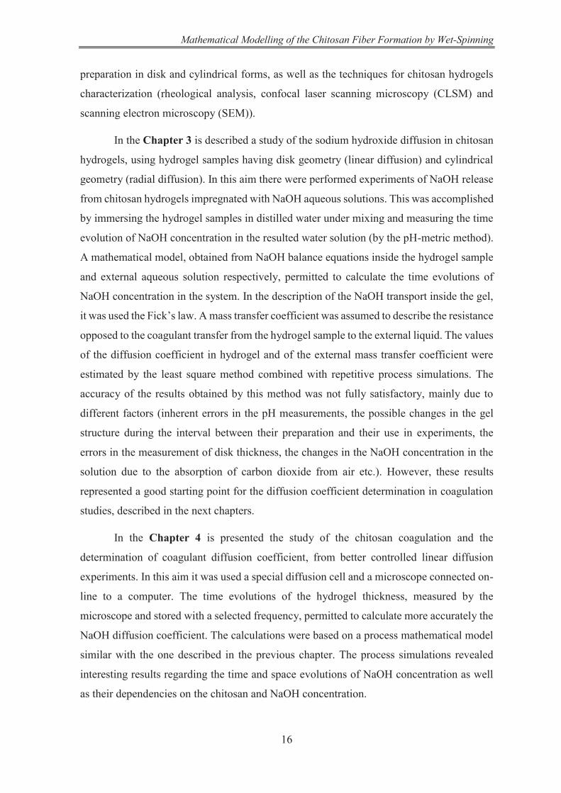
As was presented, the chitosan can be used in many fields due its biological
properties, but the main one remains the biomedical domain, as a generator of chitosan
biomaterials. The processing alternatives of the chitin and chitosan are presented in Figure
1.7.
Mathematical Modelling of the Chitosan Fiber Formation by Wet-Spinning
32
Table 1.2. Application of the chitosan (Regiel and Kyzioł, 2013).
Pharmaceutics
Gels, hydrogels (controlled drug release; Kofuji et al., 2004; Bhattarai et al., 2010) Films (drug release; Bhattarai et al., 2010) Emulsions (microspheres, microcapsules), (sustained drug release, increased
bioavailability, mucoadhesion; Dudhani and Kosaraju, 2010) Targeted cancer therapy (retention and accumulation of drug in tumor; Ta et al., 2008) Systems for controlled delivery / release of peptide drug (Prego et al., 2006), vaccines
(Illum et al., 2001), genes (Saranya et al., 2010) Medicine and biomedicine
Wound dressings, wound treatment, bandages (Atiyeh et al., 2007) Sutures, surgical implants (Bumgardner et al., 2003) Hemodialysis membranes, biomedical devices coatings (Radhakumary et al., 2012) Hemostatic (Wedmore et al., 2006), anticoagulants (Vongchan et al., 2002)
Tissue engineering Scaffolds for tissue engineering, artificial skin grafts (Ravi Kumar, 2000)
Other
Agriculture, food industry (Arora and Padua, 2010), textile industry (Raafat and Sahl, 2009), wastewater treatment (Ravi Kumar, 2000)
Figure 1.7. Alternatives of chitin and chitosan processing (Anitha, 2014).

Alin Alexandru ENACHE
33
1.2 Chitosan Hydrogels
1.2.1 Definition of a hydrogel
The first synthetic hydrogel was prepared in 1960, by Wichterie and Lim, from poly
(2-hydroxyethyl methacrylate) (PHEMA) for use as soft lenses (Kishida and Ikada, 2002).
Subsequently, new hydrogels were developed for very wide applications, especially in the
biomedical sector.
Peppas (1986), defined a gel as a “network consisting of hydrophilic polymers
capable of swelling in water or in an aqueous solution”. Guenet (1992), proposed a similar
definition: “a gel is a network consisting of interconnected polymer chains and swollen by
a solvent whose concentration is greater than 90%”.
The new definition of a gel is given by Aleman et al. (2007): “A gel is a polymer
network or a non-fluid colloidal network that is expanded throughout its whole volume by a
fluid. A hydrogel is a gel in which the swelling agent is water”.
These general definitions of the "hydrogel" term make it possible to include in this category
many materials with very different structures, physicochemical and biological properties. A
hydrogel can be defined more precisely depending on several parameters.
1.2.2 Classification of hydrogels
The hydrogels can be classified depending on the preparation methods
(homopolymers, copolymers and interpenetrating polymers), ionic charges (nonionic
hydrogels, cationic hydrogels, anionic hydrogels, ampholytic hydrogels), source (natural
hydrogels, hybrid hydrogels, synthetic hydrogels), physical properties (smart hydrogels,
conventional hydrogels), biodegradability (biodegradable hydrogels, non-biodegradable
hydrogels), crosslinking (physical crosslinked hydrogels, chemical crosslinked hydrogels).
The classification is better shown in Figure 1.8.
The chitosan hydrogels are nonionic, natural and conventional ones, which can be of
two types, following the preparation method: chemical hydrogels (crosslinked) and physical
hydrogels.

Mathematical Modelling of the Chitosan Fiber Formation by Wet-Spinning
34
Figure 1.8. Classification of hydrogels (Patel and Mequanint, 2011).
1.2.3 Chemical and physical hydrogels of chitosan
In the chemical hydrogels, the macromolecules are interlinked by covalent bonds.
The repeating units have functional groups to form the nodes or crosslinking points in
reacting with a crosslinking agent (Ross-Murphy, 1991). The crosslinking agents most
studied and used for crosslinking between chitosan chains are: glutaraldehyde, glyoxal,
diethyl squarate, oxalic acid and genipin (Berger et al., 2004a). Polymers unfunctionalized
are also used for the formation of hybrid chemical hydrogels (synthetic / natural) with
chitosan: poly (ethylene glycol) (PEG) diacrylate (Kim et al., 1995), telechelic-PVA
polymers (Crescenzi et al., 1997), or dialdehydes derived from PEG (Dal Pozzo et al., 2000),

Alin Alexandru ENACHE
35
scleroglucan (Crescenzi et al., 1995), oxidized b-cyclodextrin (Crescenzi et al., 1997) or
oxidized starch (Serrero et al., 2009).
The physical hydrogels are created by weak and partially reversible bonds. The
microstructure of the hydrogel can be stabilized by several types of reversible interactions
that are localized on "junction zones", possibly multifunctional, which can extend over a
distance between 0.1 and 1μm (Ross-Murphy, 1991). In some cases, the reversible
interactions are of high relative energy, such as the ionic bonds. In other cases, the
interactions are of low energy such as hydrogen or Van de Waals bonds, hydrophobic
interactions (Domard and Vachoud, 2001). In contrast to the covalent bonds, these bonds
are not stable because they have a certain life time. Their number and spatial distribution
fluctuate with time and temperature (Ross-Murphy, 1991). At room temperature, these
bonds have binding energy comparable to those of the group kT (Joanny, 1989). For this
reason, a reversible transition between a liquid and a gel as a function of temperature, solvent
or pH can be observed.
The chemical way for the hydrogels elaboration as a biomaterial is not a
recommended option, because it implies a structure denaturation of the chitosan and the
crosslinked agent are often toxic. Due this reason, the only way to obtain hydrogels in order
to be used as a biomaterial is the physical hydrogels from a chitosan solution without
crosslinked agent.
1.2.4 Formation of physical hydrogels based on chitosan
The physical hydrogels result from the more or less reversible interactions, coming
from: (a) ionic interactions such as ionic crosslinking and polyelectrolyte complex (PEC)
formation, or (b) weak bonds of the hydrophobic interaction and hydrogen bond type.
Depending on the type of interactions, there are different methods of preparation for physical
hydrogels. The types of the crosslinking chitosan hydrogels are presented in Figure 1.9.
1.2.4.1 Ionically crosslinked chitosan hydrogels
The crosslinker agents used in the preparation of the covalent crosslinked hydrogel,
can be found in traces and may be toxic. The preparation of the hydrogel by using the ionic
crosslinking avoid the supplementary steps of purification and verification necessary for the
hydrogels obtained by covalent crosslinking.

Mathematical Modelling of the Chitosan Fiber Formation by Wet-Spinning
36
The crosslinking implies the interaction between protonated amino units (-NH3+) and
negatively charged ions or molecules, leading to a network with ionic bridges between
polymer chains.
The ionic crosslinking is determined by the size of the crosslinking agent, as well as
the overall charge density of chitosan and of the crosslinking agent, during the reaction. The
pH during the coagulation has values between the pKa of the chitosan and the pKa of the
crosslinking agent (Berger et al., 2004a).
Figure 1.9. Structure of chitosan hydrogels; , covalent bonds; + positive groups in chitosan macromolecule; , chitosan; , additional polymer; , negative groups in
the crosslinker; , symbol for the ionic bonds (Berger et al., 2004a).
The most common application of this crosslinking technique is the formation of
nanoparticles, which are very useful for the vectorization or the release for the active
ingredients (drug delivery) (Bodmeier et al., 1989; Berthold et al., 1996; Mi et al., 1999; Shu
and Zhu, 2002). Indeed, the implementation is simple because it involves the addition drop
by drop, of the crosslinking agent using a syringe in an aqueous solution of chitosan.

Alin Alexandru ENACHE
37
1.2.4.2 Formation of polyelectrolyte complexes (PEC)
The electrostatic attraction between amino units (-NH3+) from chitosan and the
anionic moieties of other polyelectrolytes represents the principal interaction leading to the
PEC formation (Berger et al., 2004b). The complexation reaction is essentially controlled
by the entropic gain related to the release of the initially associated counter-ions to
polyelectrolytes. Tsuchida and Abe (1986), points out that there is a competition between
ionic condensation of the counter-ions and of the polyelectrolytes, but the last ones prevail
through to the cooperative interactions. This means that hydrogen bonds and hydrophobic
groups’ interactions participate also to the formation of PEC. For the preparation of a PEC,
it is not necessary to use catalysts or initiators because the reaction is carried out in an
aqueous solution; this represents an important advantage in comparison with the covalent
networks (Berger et al., 2004b). In this way the biocompatibility and bioactivity of the
material is preserved. In addition, this avoids certain purification steps before use. The most
important physicochemical factor to control is the pH of the solution which is strongly
related to the pKa of the two polyelectrolytes, but the temperature, the ionic strength (Lee et
al., 1997) and the order of the mixing are also important.
The polyanions most used with chitosan are polysaccharides which include a
carboxylic group (COO-) such as alginates (Kim et al., 1999), pectin (Yao et al., 1997),
xanthan (Dumitriu and Chornet, 2000), hyaluronic acid (Rusu-Balaita et al., 2003) and all
polysaccharides having a group sulfate such as chitosan-dextran sulfate (Schatz et al., 2004;
Drogoz et al., 2007)).
1.2.4.3 Formation of hydrophobic physical hydrogels
The gelation of chitosan is obtained by the evaporation of a hydro alcoholic solution
containing an aqueous solution of chitosan and 1,2-propanediol initially in equivalent
amounts (50:50). The mixture’s dielectric constant decreases, by the addition of the alcohol
and then by the elimination of water by evaporation, which allows to modify the dissociation
constant of the acid (acetic or hydrochloric acid) and thus hydrophilic / hydrophobic balance
of the solution. The disruption of the chain environment promotes the formation of low
energy bonds (hydrophobic interactions and hydrogen bonds) which ultimately leads to the
gelation of chitosan, by formation of an alcogel. After evaporation, these alcogels have a
positive charge of NH3+ group which is neutralized with an alkaline agent (NaOH or

Mathematical Modelling of the Chitosan Fiber Formation by Wet-Spinning
38
ammonia gas) in order to form a neutral and stable hydrogel in a hydrated medium. Physical
hydrogels obtained after neutralization and washing contain only water and chitosan. The
gels prepared by this way are rigid, translucent and transparent.
1.2.5 Gelation from an aqueous solution
1.2.5.1 Gelation from an acid aqueous solution
The gelation of chitosan from an aqueous solution consists in contacting a
concentrated polymer chitosan solution, having the concentration (cp) higher than the
critical concentration of chain entanglements (c*) with a base such ammonia (NH3) gas
vapors. In this case, the gelation takes place by the modification of the polymer ionization
state: when NH3 dissolves in the chitosan solution, it contributes to the neutralization of the
-NH3+ groups, and consequently, the reduction of the charge density of chitosan
macromolecules. The gels obtained are flexible and opaque.
Montembault et al. (2005) evidenced the existence of a second critical polymer
concentration, c**, corresponding to a molecular reorganization of the solution. As shown
in Figure 1.10, when c* < cp < c**, the solution is composed of entangled strings, whereas
for cp > c**, the strings come together to form nanoclusters. These would favor a faster
construction of the three-dimensional gel network. The authors described a similar final
morphology of the gel, when using an initial solution of polymer concentration less than
c**. The nano-objects previously described are the similar objects formed from hydrophobic
interactions and hydrogen bonds. In reality, the concentration c** is not an absolute constant
but it corresponds to a critical state reflecting the balance H / H and depending in practice
by many physicochemical parameters (DA, pH, T, etc.).
As already mentioned, the chitosan physical hydrogels prepared from aqueous
solutions are interesting because they do not contain additive that should be eliminated later.
In addition, they have the distinction of being much simpler to develop than the gels formed
in a hydro alcoholic environment.

Alin Alexandru ENACHE
39
Figure 1.10. Schematic representation of the mechanism of physical hydrogels formation
from an aqueous solution (DA = 36.7%) by neutralization with ammonia vapors (Montembault A., 2005).
1.2.5.2 Thermal gelation of chitosan in an aqueous alkali–urea solution
As mentioned in a previously paragraph, the chitosan can be dissolved in aqueous
alkali–urea solutions, due to the forming of a complex between chitosan, urea and NaOH.
The gelation occurs when the recipient filled with chitosan solution is placed in a vessel with
hot water at temperature higher than 40 °C (Duan et al., 2015). The formed complex starts
to decompose due the increase of the temperature in the chitosan solution and the chitosan
chains lose their solubility. Therefore, the chains start to associate with each other, resulting
a physical network (Li et al., 2014). The hydrogels obtained in this way are usually opaque.
Nie et al. (2016), compared the chitosan hydrogels prepared by using acid and
alkaline solvents respectively. The author found that the hydrogels via alkaline solvent are
harder than the hydrogel obtained via acid solvent. With the increasing of the hydrogel
thickness via acid solvent, the structure become rough and finally may show a fibrous

Mathematical Modelling of the Chitosan Fiber Formation by Wet-Spinning
40
structure. Significantly different from the acidic system, alkaline system evolves in its
entirety (Figure 1.11).
Figure 1.11. Observation of the gelation process by confocal laser scanning fluorescence microscope (CLSM). (a) via acidic solvent, scale bar - 50 μm; (b) via alkaline solvent,
scale bar-100 μm; c(CS) = 2 wt.% (Nie et al., 2016).
1.3 Chitosan fibers
1.3.1 Overview of fiber
1.3.1.1 Definition
A textile fiber is defined as a solid having a preferred dimension in one direction and
for which a length and a diameter can be defined. Specifically, a fiber is characterized by a
length to diameter ratio higher than 100 (Hagège, 2004).
The fiber should be distinguished from the wire, which can be in the following forms:
1. a number of fibers twisted together (spun);
2. a number of filaments held together with or without twisting (non-twisted yarn);
3. a single filament with or without torsion (a monofilament);

Alin Alexandru ENACHE
41
4. a narrow ribbon of material, such as paper, synthetic polymer filaments, or metal sheets,
with or without twist, for textile construction.
A representation of fibrous exoskeleton material structure is presented in Figure
1.12.
Figure 1.12. Exoskeleton material structure (Rabbe et al., 2005).
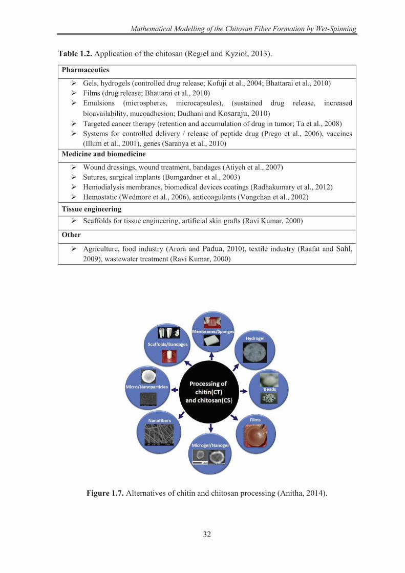
1.3.1.2 Classification
There are many possible criteria for textile fibers classification: their origin, their
method of manufacture, their chemical constitution or their areas of use. First, textile fibers
can be classified into two groups according to their origin and their method of production
(Cook, 1968): natural fibers and hand-man-made fibers. The natural fibers are subdivided
into three large groups according to their origin: plant (cotton, kapok, flax, hemp, jute, ramie,
sisal etc.), animal (hair, silk etc.) or mineral (asbestos, glass, carbon etc.). The hand-man-
made fibers can be subdivided into two classes: fibers derived from a natural polymer, such
as cellulose, chitin or chitosan or from proteins (called “artificial fibers”) and fibers made
from a synthetic polymer, such as polyesters or polyamides. The classification of the fibers,
proposed by Cook (1968) is presented in Figure 1.13.
Their chemical constitution can be another classification criterion (Hagège, 2004).
According with this criterion the fibers can be divided in organic and inorganic fibers.
The organic fibers include: the family of natural polymers (wool, cotton, silk, chitin,
cellulose derivatives etc.); the family of "conventional" synthetic polymers (polyamides,
Mathematical Modelling of the Chitosan Fiber Formation by Wet-Spinning
42
PET and other polyesters, acrylics, polyolefins, PTFE or polyurethanes); the family of new
synthetic polymers (polyether ether ketones (PEEK), polyimides or polybenzimidazole).
Figure 1.13. Classification of the fibers (Cook, 1968).
The inorganic fibers consist of glass, carbon, ceramics (other than glass and similar),
metals etc.
The chitosan fibers are called “artificial natural” fibers because those are obtained
from a natural polymer by using a spinning process.
1.3.2 Production of chitosan fibers
The chitosan fibers can be obtained by three technologies: wet spinning, dry-jet wet
spinning and electrospinning. A short description of each method is presented below.
1.3.2.1 Wet spinning of chitosan
The first studies for the chitosan spinning was made by Rigby (1936), who dissolved
3.8% (w/w) of the polymer in 1.2% aqueous solution of acetic acid. The fibers were obtained
by extrusion of the collodion (chitosan solution) so prepared, in a coagulation bath consisting
of 93% water, 4.6% of sodium acetate, 2% sodium hydroxide and 0.2% sodium dodecyl

Alin Alexandru ENACHE
43
sulfate, followed by washing and drying under tension. The fibers are described as being
tough, flexible and brilliant, without any result of mechanical properties being specified.
Other spinning tests have been reported by Ming (1960), who dissolved the 0.5%
solution of acetic acid in order to obtain a collodion with 5-6 % (w/v). The coagulation bath
contained 100 parts water, 2 to 2.5 parts NaOH, 15 parts glycerin and an undescribed amount
of sodium sulfate. He added to the collodion 2 parts of zinc acetate, 4 of glycerin and 0.5 of
alcohol to improve its stability.
Mitsubishi Rayon (Ootani et al., 1981), published a patent describing the following
method: the collodion, containing 3% chitosan dissolved in a 0.5% aqueous acetic acid
solution, is extruded in a bath, containing a 5% aqueous solution in NaOH.
In Table 1.3 are illustrated the solvents and the coagulating agents used in the studies
of chitosan wet-spinning before 1990.
Since 1990, the authors have tried to optimize the different parameters of spinning
(composition of the collodion, coagulation bath, stretching, post-treatment) for the purpose
to improve the mechanical properties of the chitosan fibers obtained.
A scheme of the chitosan wet spinning process is presented in Figure 1.14.
Figure 1.14. A scheme of the chitosan wet spinning process (Knaul, 1998).
The chitosan wet spinning process implies several stages. The first is the
solubilization of the chitosan (the obtained solution is also called “collodion”) followed by
passing of the collodion through a spinneret immersed in the coagulation bath. The spinning

Mathematical Modelling of the Chitosan Fiber Formation by Wet-Spinning
44
collodion starts to gelate in contact with the coagulation agent, during its passage through
the coagulation bath. The next step is the washing (removing the coagulation agent) of the
filament followed by the drying of the filament in order to eliminate the contained liquid.
Finally, the fiber is winding on a reel.
Table 1.3. First trials of chitosan wet spinning
Year Reference Solvent Coagulation bath
1936 Rigby (1936) 1.2 % acetic acid aqueous
solution
4.6% sodium acetate 2% sodium hydroxide
0.2% sodium dodecyl sulfate
1960 Ming (1960)
0.5 % acetic acid aqueous solution
2 parts of zinc acetate, 4 parts of glycerin and
0.5 parts of alcohol
100 parts water 2 to 2.5 parts NaOH,
15 parts glycerin X parts of sodium sulfate
1980 Ootani et al.
(MitsubishiRayon) (1980)
0.5 % acetic acid aqueous solution 5% NaOH aqueous solution
1981 Ootani et al.
(Mitsubishi Rayon) (1981)
1% acetic acid aqueous solution
2% dodecyl sulfate de sodium aqueous solution
1984 Tokura and Seo (Fuji Spinning)
(1984)
dichloroacetic acid aqueous solution
CuCO3-NH4OH aqueous solution
1985 Kurahashi and Seo I.
(Fuji Spinning) (1985)
dichloroacetic acid aqueous solution
5 to 20 % sodium hydroxide aqueous solution
+ NaOH/methanol
1987 Tokura et al. (1987). 2-4 % acetic acid aqueous solution
1) 2M CuSO4: NH4OH (1: 1 v/v)
2) mixture 5% NaOH: 70:30 v / v ethanol
3) 2M CuSO4: 1M H2SO4 + other treatments:
1) and 3) 50% ethanol aqueous solution + 0.2M EDTA • 4Na
2) 50% ethanol aqueous solution
1.3.2.2 Dry-jet wet spinning of chitosan
This method was used for the spinning of the cellulose in N-oxide hydrates of N-
methyl morpholine (Kim et al., 2002) or in polyamic acid solutions (Park, 2001), but was
less used for chitosan spinning.

Alin Alexandru ENACHE
45
The dry-jet wet spinning is a mixing between the wet spinning and dry spinning. In
this case the collodion is not extruded directly in the coagulation bath, but it passes a distance
in air before entering in the coagulation bath. The solution state is therefore maintained on
a certain length (usually few centimeters) on which important internal restructuring can take
place.
Kwon et al. (1999) and Lee (2000), emphasized the importance of the length of the
air gap between the spinneret and the coagulation bath and the "dry-jet ratio". From a
collodion of chitosan acetate at 5% by mass and an air atmosphere length of up to 5 cm, they
succeed in obtaining fibers of tenacity equal to 2.11 g / denier with an elongation at break
between 8 and 13%. It seems that stretching at the outlet of the spinneret before coagulation
also makes it possible to improve the mechanical properties since the tenacity of the fibers
is one of the highest values found in the literature. Agboh and Qin (1992), mentioned that
the stretched chitosan fibers obtained by this method generally have a very high degree of
orientation but no details are provided on the degree of crystallinity of the fibers.
1.3.2.3 Electrospinning of chitosan
The electrospinning (Li and Xia., 2004) is a particular method using electrostatic
forces to form polymer nanofibers. A classic electrospinning setup consists of 3 major
components: a metal spinneret, a metal collector (plate) and a high voltage generator (Figure
1.15). The principle of the method consists in applying an electric field at the outlet of the
spinneret to create electrically charged polymer solution jets which are then collected on the
receiving screen placed at about fifteen centimeters from the spinneret exit in the form of a
nonwoven web. During the process, the liquid jet is continuously stretched, the solvent
evaporates and the fiber diameter can be reduced from several hundred microns to about ten
nanometers. The properties of the fibers obtained by the electrospinning method are
depending both on working conditions (voltage, distance between the spinneret and
collectors, solution feed rate etc.) and chitosan solution properties (viscosity, average molar
weight, conductivity and surface tension) (Geng et al., 2005).

Mathematical Modelling of the Chitosan Fiber Formation by Wet-Spinning
46
Figure 1.15. Schema of electrospinning technology (Terada et al., 2012).
A number of studies report innovations and results in the chitosan electrospinning
(Bhattarai et al., 2005; Geng et al., 2005; Pillai and Sharma, 2009). However, this method
only makes it possible to obtain chitosan nanofibers in the form of a nonwoven and thus
limits the possible applications of these fibers. Presently, investigations regarding the
development and applications of woven or knitted chitosan textiles are in progress.
1.4 Diffusion in polymer solutions and hydrogels
1.4.1 Introduction
The diffusion is the movement process of a substance from a region (rich in this
substance) to another part of the system (poor in the substance) (Crank, 1975). The
movement is due the random molecular motions. The diffusion depends on temperature,
pressure, viscosity and solute size. The diffusion is fast in gaseous phase, slower (several
hundred times) in liquid phase and much slower in solid phase (Cussler, 1997). In polymers
and hydrogels, the diffusion process is complex and its rate is placed between the rates in
liquid and solid.
In the study of the diffusion processes, very often is used the Fick's first law,
quantitatively described by the Equation (1.3).
(1.3) zCDj

Alin Alexandru ENACHE
47
Alfrey et al. (1966) observed and reported two types of solvent diffusional transport
in polymers: Fickian diffusion (Type I) and non-Fickian diffusion (Type II and the
anomalous) respectively. These types are distinguished by taking as criteria the intensity of
solvent diffusion and relaxation rate of the polymer. Generally, the mass of the solvent
absorbed into a polymer, during the time t, reported to the unit of area, is given by the
expression (Massaro and Zhu, 1999):
ntM kt (1.4)
where k is a constant, t is time and n is a parameter depending on the diffusion mechanism,
which takes values between 0.5 and 1.
1.4.1.1 Fickian diffusion
The Fickian diffusion occurs in a polymer, when this is in rubbery state (the
temperature is higher than the glass transition value, Tg), the polymer chains having a higher
mobility, allowing the solvent to penetrate easier the polymer network (Grinsted R. A.,
1992). The diffusion rate is slower than the polymer relaxation rate (Rdiffusion << Rrelaxation).
The diffusion distance is proportional to the square-root of time, in equation (1.4), n=1/2,
this taking the form (1.5) (Quin W., 1993). The Fickian diffusion occurs also in polymer
networks below Tg, in the presence of plasticizers.
1/2tM kt (1.5)
1.4.1.2 Non-Fickian diffusion
The Non-Fickian diffusion occurs in polymer networks, when the polymer chains
are not sufficiently mobile (the temperature is below the glass transition temperature Tg) and
the solvent diffuse slowly. The Non-Fickian diffusion includes the Type II diffusion
(diffusion rate is quicker than the polymer relaxation Rdiffusion >> Rrelaxation) and the so called
‘anomalous diffusion’ (diffusion rate has the same order with the polymer relaxation process
Rdiffusion ~ Rrelaxation). If, in relation (1.4), n=1, the process is considered Case II diffusion and
if ½ < n < 1 the diffusion process is considered an anomalous diffusion.
The usual experimental techniques used to study the diffusion processes in polymers
are the gravimetric method (Langdon and Thomas, 1971), the membrane permeation

Mathematical Modelling of the Chitosan Fiber Formation by Wet-Spinning
48
(Griffiths et al., 1995), fluorescence (Mackie and Meares, 1955) and dynamic light scattering
(Nyström et al., 1981).
1.4.2 Diffusion models and theories
There were proposed several theories and physical models to describe the diffusion
process in polymer solutions and gels: free volume models, obstruction effects models,
hydrodynamic theories, combined obstruction and hydrodynamic effects etc.
1.4.2.1 Theory of the free volume
These models were firstly proposed by Cohen and Turnbull (1959). The solute
diffusion takes place by jumps between the void spaces appeared by the redistribution of
free volume within the liquid (in the hypothesis that the free volume redistribution is not
accompanied by any change of energy). These holes are then refilled by an opposite process
(Vrentas and Duda, 1977).
1.4.2.1.1 Fujita’s model
Fujita was the first who proposed a diffusion model for polymers, based on the free
volume theory (Fujita, 1961). He studied the diffusion of a plasticizer molecule in a system
including the solvent and the polymer. Fujita used the theory of Cohen, which defines the
probability, P(υ*), to find in a liquid, holes of volume υ*, for identical molecules of
plasticizer.
expV
bP Af
(1.6)
A - a constant parameter; b - numerical factor (~1); fV - the average free volume per
molecule.
The diffusion model proposed by Fujita is founded on the following hypothesis:
(1) the diffusion phenomenon takes place due to the free volume rearrangement within the
polymer structure;
(2) the reorganization of the free volume spaces occurs without change of energy;

Alin Alexandru ENACHE
49
(3) the diffusion phenomenon occurs only if the free volume exceeds a minimum value, υ*;
(4) for a diffusing molecule, the diffusion intensity is directly proportional to the probability
P(υ*), to find a space having a minimum volume υ*.
The mobility is defined by the Equation (1.7) (Massaro and Zhu, 1999):
expefV
BD ARTf
(1.7)
T – temperature; A – a preexponential constant; R – ideal gas constant; B – parameter
depending on the diffusing molecule dimension.
The model of Fujita is recommended for processes of small molecules diffusion in
small concentration polymer solutions and gels (typically organic substances).
1.4.2.1.2 The model of Yasuda et al.
Yasuda et al. (1968) studied the diffusion process of NaCl in various hydrophilic
polymer systems by using the free volume theory, formulating the expression:
0
1exp 11
ef
V P
D BD f
(1.8)
D0 - solute diffusion coefficient in liquid without polymer; fV* - free volume of the solvent
in polymer solution; φp – polymer fraction (vol.) in solution; B – parameter depending on
the diffusing molecule dimension.
As the model of Fujita, the Yasuda’s model is recommended for processes of small
molecules diffusion in small concentration polymer solutions and gels.
1.4.2.1.3 The model proposed by Vrentas and Duda
A more complicated model based on the free volume theory is that formulated by
Vrentas and Duda (see Massaro and Zhu, 1999). This model describes the diffusion
coefficient dependencies in respect with physical properties of the diffusing system: working
temperature, the activation energy of the diffusion process, the concentration of the polymer,
the dimension of the solvent molecule and the properties of diffusant molecule. In accord

Mathematical Modelling of the Chitosan Fiber Formation by Wet-Spinning
50
with Vrentas and Duda, the diffusion coefficient in the polymer solution is defined by the
expression:
1 1 2 201
11 1 21 1 12 2 22 2
1 2
ˆ ˆexp expef
g g
V VED DRT K K T T K K T T
(1.9)
D01 – represents the solvent self-diffusion coefficient in liquid solution, in absence of
polymer; E – diffusion activation energy; - characteristic volumes; ω1, ω2 - mass
fractions; γ1, γ2 - overlapping factors; ξ - volume ratio of the jumping units (solvent to
polymer), Tg1, Tg2 - glass transition temperatures; K11, K21, K12, K22 – free volume
parameters;
K11 and K21 are calculated from the Equations (1.10) and (1.11).
011 1 1 1 1 1
ˆ 1 Gg H cK V T f (1.10)
121
1 1 11
GH
GH c
fKf
(1.11)
α1 and αc1 - thermal dilatation coefficients for solvent and for the ensembles of occupied and
free volumes respectively; - free volume occupied by the solvent at 0 K; - average
fractional hole free volume. The model of Fujita appeared as a special case of the more
complicated model proposed by Vrentas and Duda.
The model of Vrentas and Duda can be applied on the diffusion of organic solvents
in polymer solutions. However, its utilization is demanding the values of an important
number of specific parameters.
1.4.2.2 Models based on the obstruction effects
The models of this class are hypothesizing that the polymer chains in polymer
solutions or gels are impenetrable and have static positions in respect with the diffusing
molecules. As result it is appearing an increase of the trajectory traveled by the diffusing
molecules, forced to bypass the polymer ones (Amsden, 2002).
* *1 2ˆ ˆ,V V
01̂V G
Hf 1

Alin Alexandru ENACHE
51
1.4.2.2.1 The Maxwell–Fricke model
In accord with this model, the diffusion coefficient is calculated by the Equation
(1.12):
0
1 1 ''1
efDD
(1.12)
Def - effective diffusion coefficient; D0 - diffusion coefficient in solvent without polymer; φ
- polymer volume fraction; φ’ - volume fraction of the polymer plus non-diffusing solvent
bound to the polymer; χ – shape factor of solvent (1.5 for rods and 2.0 for spheres).
The Maxwell–Fricke model is recommended for the diffusion systems involving
small molecules in polymer solutions having small polymer concentrations.
1.4.2.2.2 The model of Mackie and Meares
The authors of this model used the theory formulated by Fricke for the electrolytes
diffusion in resin membranes. They hypothesized that the polymer mobility is negligible in
respect with those of ions and water. As mentioned above, during the diffusion in a polymer
solution, the presence of polymer macromolecules, acting as obstacles, are inducing an
increase of the distance travelled by the diffusing particles. According to this model, the
effective diffusion coefficient of a relatively small particle, can be evaluated by the Equation
(1.13):
2
0
11
efDD
(1.13)
In this expression, the notations have the same significances as in the expression (1.12).
1.4.2.2.3 The model of Wang
A first equation for prediction of diffusion coefficients in gels was proposed by
Wang (Lauffer, 1961; Westrin et al., 1994), assuming that the decrease of diffusion

Mathematical Modelling of the Chitosan Fiber Formation by Wet-Spinning
52
coefficient in a gel, as compared to that in the free solution, is proportional to the volume
fraction of the polymer in the gel:
0
1efDD
(1.14)
Def, D0 and φ have the same significances as in previous relations; α – shape parameter (1.5
for prolate; 3 for oblate ellipsoids; 1.67 for randomly oriented rods (Lauffer, 1961; Massaro
and Zhu, 1999).
1.4.2.2.4 The model of Ogston et al.
The authors considered the polymer macromolecules as obstacles similar with a
fascicle of randomly distributed fibers of molecular size. Accordingly, the effective
diffusion coefficient for a diffusant molecule will depend on the characteristics of these
obstacles, as well as on the properties of the diffusant and can be calculated by the Equation
1.15 (Massaro and Zhu, 1999).
1/2
0
expef hD RD
(1.15)
φ - polymer volume fraction in the solution; Rh - hydrodynamic radius of the diffusing
molecule; ρ- radius of the cylindrical fiber.
1.4.2.2.5 Hard sphere theory
This theory was formulated by Johansson et al. (1991) assuming spherical shaped
solute particles in polymer solutions and gels. The main hypotheses of the proposed model
are the following:
(1) in the diffusing medium, the diminution of solute diffusion coefficient is due to the steric
hindrance, the hydrodynamic interferences being unimportant;
(2) the steric hindrance is generated only by the polymer macromolecules motionless grid;
(3) the diffusing grid is structured as a set of cylindrical spaces (cells).
Based on these assumptions, the expression deduced for the calculation of the
diffusion coefficient has the form:

Alin Alexandru ENACHE
53
21
0
2efDe e E
D (1.16)
α - parameter calculated by the relation: 2
2hR
(1.17)
φ - polymer volume fraction; ρ - polymer radius; Rh – hydrodynamic radius of the diffusing
molecule. E1 is the exponential integral having the expression:
1
u
x
eE x duu
(1.18)
1.4.2.3 Hydrodynamic theories
The models of this class are founded using the Stokes-Einstein theory of diffusivity.
The main assumptions regard the shape of the solute molecule, considered as a hard sphere
much larger than the solvent molecules where it is moving. Also, it is assumed that the solute
moving, into the solvent medium, occurs with a constant velocity and is struggled by a
frictional force (Amsden, 2002). The main relations for calculus of diffusion coefficient
deduced by this type of models are given in Table 1.4.
Table 1.4. Main relations for calculus of diffusion coefficient deduced using hydrodynamic theories.
Model Expression Model name
Cukier’s model 0
1efh
DkR
D Cukier (1984)
Model of Altenberger
and Tirrell 1/2
0 expefD D c Altenberger and Tirrell
(1984)
Phillies’ model 0 expefD D c Massaro and Zhu (1999)
As a conclusion, it can be stated that the diffusion process in polymers and hydrogels
was studied by many authors. There exist many models and theories aiming to describe the
diffusion process. Some models take into account the physical properties of the studied
system other take into account the interaction between the components of the system. All
the models have the applicability and restraints and it is necessary to take into account these

Mathematical Modelling of the Chitosan Fiber Formation by Wet-Spinning
54
when a model is used. A model which can be used for all systems and for all concentration
ranges does not exist, but all these have been obtained starting from the Fick’s first law.

Alin Alexandru ENACHE
55
EXPERIMENTAL METHODS USED IN
THE CHITOSAN HYDROGELS PREPARATION
AND CHARACTERIZATION

Mathematical Modelling of the Chitosan Fiber Formation by Wet-Spinning
56
Introduction
In this chapter are described the experimental techniques and procedures used in the
thesis: the chitosan’s purification, chitosan characterization (determination of the average
molar weight, the degree of acetylation, the water content in dry chitosan), preparation of
the chitosan solutions, determination of the real concentration of chitosan solutions,
determination of the viscosity of chitosan solutions, methods of obtaining the chitosan
hydrogel in disk and cylindrical forms and some analysis made on chitosan hydrogels
(characterization of the mechanical properties of the chitosan hydrogels using the rheology,
confocal laser scanning microscopy (CLSM) and scanning electron microscopy (SEM)).
2.1 Chitosan purification
The necessary amount of chitosan was dissolved (concentration around 0.5 wt. %)
in an aqueous solution of acetic acid (providing a stoichiometric amount of acetic acid
necessary to protonate the chitosan amino groups). The solution was kept under mixing
during one night to ensure that all chitosan was dissolved. Further, the solution was
consecutively filtered on three cellulose acetate membranes having the pore dimensions 3
μm, 0.80 μm and 0.45 μm respectively, using a column with compressed air, working at 3
bars. Next, ammonia solution was added up until the pH was 9, in order to precipitate all
the chitosan. Then repeatedly washed with deionized water and centrifuged until the pH was
neutral. Finally, the chitosan precipitate was immersed in freezer for one night and then
immersed and left for three days in dry freezer. During this stage, the chitosan is freeze
drying.
2.2 Chitosan characterization
2.2.1 Determination of the degree of acetylation
The degree of acetylation was determined using the 1H nuclear magnetic resonance
(NMR) spectroscopy analysis. The analysis sample was prepared by dissolving 1.67 mg
chitosan in 2 mL solution of deuterated water, containing hydrochloric acid (0.5 % w/w).
The sample was analyzed in a Bruker 250 spectrometer at 25°C. An example of spectra is
presented in Figure 2.1. According to Hirai et al. (1991), the degree of acetylation was
calculated from the recorded spectra, using the equation (2.1). This is the ratio of the area of

Alin Alexandru ENACHE
57
the methyl protons of the N-acetyl glucosamine residues to that of all of the H2 to H6 protons
of both glucosamine and N-acetyl glucosamine. In this way, the DA value for the used
chitosan was found to be approximately 2.8%.
3
2 6
1 1 0.0903 3100 100 2.82%1 1 0.6385
6 6
CH
H H
IDA
I (2.1)
Figure 2.1. The chitosan spectra recorded by Bruker 250 spectrometer.
2.2.2 The average molar weight (Mw)
The average molar weight was determined by using the size exclusion
chromatography (SEC) coupled with LC pump (Spectra Physics) feeding the Protein Pack
glass 200 SW and TSK gel 6000 PW columns. The solution was obtained by dissolving 4
mg chitosan in 4 mg acid solution (pH 4.5). Before injection, this was filtered, using a 0.45
μm pore size membrane. The spectrum obtained is presented in Figure 2.2. The value of
average molar weight for the chitosan determined by this method was Mw = 5.446·105 (± 10
000) g/mol.

Mathematical Modelling of the Chitosan Fiber Formation by Wet-Spinning
58
Figure 2.2. The elution diagram obtained from the size exclusion chromatography (SEC).
2.2.3 Water content
The water content of chitosan was determined by Thermogravimetric Analysis. In
this aim it was used a thermogravimetric analyzer, DuPont Instrument 2950. The
temperature was increased from 30°C to 210°C with a ramp of temperature of 4°C/min. The
chitosan thermogravimetric diagram is presented in Figure 2.3. The water content of
chitosan was found to be approximately 7%.
Figure 2.3. Thermogravimetry diagram for a chitosan lyophilizate

Alin Alexandru ENACHE
59
2.3 Preparation of the chitosan solution
In order to obtain a final chitosan solution having a chitosan concentration around w
% (in weight), w g of chitosan was weighed and added to 120 mL water into a vessel
provided with mechanical mixing (theoretically, the volume of water should be ~100 mL
but in order to compensate the water evaporation during the mixing, it is necessarily to add
~ 20 % volumetric extra water). Finally, a stoichiometric volume of glacial acetic acid was
added (659 μL, calculated using the equations (2.2) and (2.3)) in order to protonate the amino
sites in accordance with the degree of acetylation. The solution was kept at room temperature
under mixing (50 rpm) over the night (approximately 18 hours). Next, the obtained chitosan
solution (collodion) was centrifuged for 10 minutes at 5000 rpm, in order to eliminate the
air bubbles. In Table 2.1 are presented the properties of the chitosan used in this study.
Table 2.1. Chitosan characteristics.
Number-average molar weight of chitosan ( ) 397 +/- 10 kg/mol
Weight-average molar weight of chitosan ( ) 547 kg/ mol +/- 10 kg/mol
Solid chitosan density 1200 kg/m3
Water content in chitosan powder 7 +/- 0.5 wt. %
Degree of acetylation 2.82 +/-0.5 %
Number of ‘amino’ groups per chitosan chain ( ) 2340 groups /molecule
1 1chitosan water AcOHAcOH
av
m DA H Mm
M (2.2)
(2.3)
1av GlcNAc GlcNM M DA M DA (2.4)
mAcOH - mass of acetic acid (g);
mchitosan – mass of chitosan (in the considered example, 2 g);
DA – degree of acetylation of chitosan (as a fraction);
Hwater – water concentration in chitosan (mass fraction);
MAcOH – Molar weight of acetic acid (60.06 g / mol);
Mav – an averaged molar weight of the two units in the chitosan macromolecule (2-
acetamido-2-deoxy-d-glucopyranose and 2-amino-2-deoxy-d-glucopyranose) (g / mol);
nM
wM
+3NH
n
AcOH
AcOHAcOH
mV

Mathematical Modelling of the Chitosan Fiber Formation by Wet-Spinning
60
MGlcNAc – Molar weight of the 2-acetamido-2-deoxy-d-glucopyranose
MGlcN – Molar weight of the 2-amino-2-deoxy-d-glucopyranose.
As it was presented above, the volume of water was in excess in order to compensate
the water evaporation during the mixing. The real concentration of the chitosan solution is
unknown so it is necessary to be determined precisely. A thermogravimetric method was
again used in order to measure the real concentration in the lyophilizate prepared from the
solution (collodion). Four chitosan solutions (1.5 %, 2%, 2.5% and 3%) were prepared using
10 % volumetric extra water. The Petri dishes were weighted and filled with chitosan
solutions. The ensemble Petri dish and chitosan solution was reweighted. The weights of the
chitosan solutions were determined as the differences between the weights of the ensembles
and those of empty Petri dishes. Subsequently, the filled Petri dishes were placed in freeze
dryer for three days in order to remove the water content. Finally, the ensemble Petri dish
and dry chitosan was reweighted and the amount of the dry chitosan was determined. The
results are shown in Table 2.2.
Table 2.2. Determination of real concentrations of the prepared chitosan solutions.
Envisaged conc.
[wt %]
Dish, [g]
Ensemble, [g]
Chitosan solution, [g]
Dry ensemble [g]
Dry chitosan,
[g]
Real conc. [wt %]
3 1.945
1 5.9724 4.0273 2.0842 0.1294 3.21
2.5 1.944
7 5.4012 3.4565 2.0461 0.0943 2.73
2 1.940
2 8.2745 6.3343 2.0911 0.1403 2.22
1.5 1.902
3 8.0541 6.1518 2.0104 0.1005 1.63
In the processes of fiber and cylindrical hydrogel formation, it was observed a
difference between the diameter of the spinneret orifice (the device through which is forced
to pass the chitosan solution in order to obtain a fiber) and the resulted cylindrical hydrogel
diameter. When the aqueous acetate chitosan solution leaves the spinneret, a swelling
phenomenon occurs due the high viscosity of the spinning solution. The aim of this
paragraph was to determine the influence of the spinneret diameter and the injection’s
pressure in final fiber’s diameter. In order to analyze this phenomenon, three spinnerets

Alin Alexandru ENACHE
61
0.023” (0.5842 mm), 0.033” (0.8382 mm) and 0.063” (1.6002 mm) in internal diameter were
used. The spinneret was attached to a syringe that contained aqueous acetate chitosan
solution and all the ensemble was immersed into a beaker filled with 1M sodium hydroxide
solution (coagulation bath). The working injection pressure was set up (1.5 bar, 1.75 bar and
2 bars) and the injection was carried out using a foot lever. After a given time
(approximatively 5 minutes), the chitosan fiber was removed from the coagulation bath and
the external diameter was measured under Leica M205A stereo microscope. The results are
presented in Figures 2.4 and 2.5.
Figure 2.4. The influence of the spinneret diameter on the final fiber’s diameter.
Figure 2.5. The influence of the injection pressure on the final fiber’s diameter.
0
0.5
1
1.5
2
2.5
3
0.5 0.7 0.9 1.1 1.3 1.5 1.7
fiber
dia
met
er,
mm
spinneret diameter, mm
1.5 bar 1.75 bar 2 bar
0
0.5
1
1.5
2
2.5
3
1.3 1.5 1.7 1.9 2.1
fiber
dia
met
er, m
m
pressure, bar
0.5842 mm (0.023") 0.8382 mm (0.033") 1.6002 mm (0.063")

Mathematical Modelling of the Chitosan Fiber Formation by Wet-Spinning
62
In Figure 2.4, approximately a linear dependence between the spinneret diameter and
the final fiber diameter can be observed. Also, in Figure 2.5 approximately a linear
dependence between the injection pressure and the final fiber diameter can be observed as
well.
2.4 Determination of the chitosan solutions viscosity
The viscosities of the chitosan solutions were measured in continuous mode, using a
rheometer AR2000Ex (TA Instruments), with cone-plane geometry. The measurements
were performed at 20 °C in the shear rates interval 0.01 - 100 s-1. The results were analyzed
in TRIOS software by TA Instruments. The Cross model (Equation 2.5) was used in order
to determine the zero-rate viscosity of the chitosan solutions.
011 m
c1 m (2.5)
where η is the viscosity, η0 the viscosity at zero shear rate, γ̇ the shear rate, α the relaxation
time (consistency) of the polymer chains in the solution and the parameter characterizes
the pseudo plasticity of the material (here it is connected to the disentanglement of chitosan
chains) (Krieger, 2014).
Like other polysaccharide solutions, the chitosan solutions are pseudo plastic (Picout
and Ross-Murphy, 2003): at low shear rates, the viscosity is not depending on shear
(Newtonian plateau), the chitosan solution exhibiting a Newtonian behavior; but at high
shear rates (higher than a critical value 1/ c), the viscosity decreases significantly (Figure
2.6). An example of the determination of the viscosity at zero-rate is shown in Figure 2.6.
The viscosity of the solution on the Newtonian plateau (viscosity at zero shear rate, η0) and
the critical shear rate γ̇ will depend on the polymer concentration, its molar weight,
temperature, the nature of the solvent and the ionic strength (Desbrieres, 2002; Cho et al.,
2006).
The fitted function using the Cross model was used to determine the viscosity at zero
share rate, by using the TRIOS software.
The dependence of the viscosity at zero shear rate (η0) on the chitosan concentration
(Cp) is given in Table 2.3 and illustrated graphically in Figure 2.7.

Alin Alexandru ENACHE
63
Figure 2.6. Viscosity rate (η) of a chitosan solution (2.5 wt. %) versus the shear rate (γ̇); the points (●) represents the experimental values; - the continuous line represents the
prediction by the Cross model.
Figure 2.7. Viscosity at zero shear rate (η0) versus the chitosan concentration (Cp, wt. %).
0
100
200
300
400
500
600
700
800
0 0.5 1 1.5 2 2.5 3 3.5 4
η 0(P
a.s)
Cp (%)

Mathematical Modelling of the Chitosan Fiber Formation by Wet-Spinning
64
Table 2.3. The zero-rate viscosity of the aqueous acetate chitosan solutions.
Chitosan concentration, % Viscosity η, Pa·s Consistency αc, s 1.00 1.71 0.040
1.50 13.30 0.162
2.00 69.27 0.595
2.50 179.21 1.55
3.00 365.52 4.67
3.50 710.80 7.95
2.5 Physical chitosan hydrogels preparation
2.5.1 Chitosan coagulation
As already shown, the chitosan is soluble in acid solutions. The most used
solubilization agent is the acetic acid. In order to prepare a chitosan solution, the acid is
added in stoichiometric amount in order to protonate all the amino groups of the chitosan
molecules. According to Rinaudo (1999) the pH of the acid polymer solution should be
between 4.5 and 5. Chenite et al. (1999) reported that the chitosan remains in solution until
the pH is under 6.2, over this pH, the first precipitates (chitosan aggregates or chitosan
crystals) starting to appear. The range of pH necessary for neutralization of -NH3+ groups is
between 6.2 and 7.4. The most used base for chitosan coagulating is sodium hydroxide. The
chemical mechanism of chitosan solubilization and coagulation can be resumed as in Figure
2.8.
Figure 2.8. The mechanism of chitosan coagulation (Ch a chitosan molecule).
The overall mechanism of chitosan coagulation is complex and not fully proven. It
results from the diffusion of the base, the neutralization of chains and their association
forming the gel. This involves many parameters such as polymer concentration, degree of
acetylation, average molar weight, the nature of coagulation agent, concentration of
coagulation agent, temperature of the coagulation bath.

Alin Alexandru ENACHE
65
2.5.2 Chitosan hydrogel with disk geometry
The chitosan hydrogels in disk form (necessary in diffusion study described in
Chapter 3) are obtained by using Petri dishes with 30 mm diameter. The Petri dishes were
filled with the chitosan solution prepared as described above. The Petri dishes were
immersed into a Berzelius glass containing sodium hydroxide aqueous solution and left a
set time so that a chitosan hydrogel is obtained. After the desired coagulating time, the Petri
dish was removed from the sodium hydroxide solution. The uncoagulated chitosan solution
was removed and the hydrogel was placed into a Berzelius glass with deionized water in
order to wash out the sodium hydroxide. The washing was carried out until the pH of the
hydrogel supernatant was neutral. The block diagram of the hydrogel preparation process is
presented in Figure 2.9. The process is also shown in Figure 2.10.
Figure 2.9. The block diagram of the hydrogel preparation process.

Mathematical Modelling of the Chitosan Fiber Formation by Wet-Spinning
66
Figure 2.10. Scheme of hydrogel chitosan formation in disk form after partial neutralization of chitosan solutions.
2.5.3 Chitosan hydrogel with cylindrical geometry
An amount of chitosan acidic solution was introduced into a syringe pump connected
to a compressed air device. The device has the possibility to modify the flow rate of the
chitosan solution by tuning the pressure of the output air. The syringe pump was immersed
into a Berzelius glass containing sodium hydroxide aqueous solution. Further, the chitosan
solution was injected through the spinneret into the liquid coagulation bath. When attained
the desired length of the sample, the pumping was stopped and the coagulation continued.
After a given coagulation time, sufficiently long to insure the complete coagulation
(approximately 10 minutes), the cylindrical chitosan gel so obtained was extracted from the
solution and cut with the aid of scissors. In order to homogenize the concentration of sodium
hydroxide into the vessel, a magnetic stirrer, set up at 400 rpm, was used.
Finally, the hydrogel cylinder was removed from the coagulating bath and washed
to neutral pH, with deionized water. The scheme of the coagulation process is shown in
Figure 2.11.

Alin Alexandru ENACHE
67
Figure 2.11. Scheme showing the hydrogel chitosan preparation in cylindrical form.
2.6 Characterization of the mechanical properties of the chitosan hydrogels
The measurements were carried using disk shape chitosan hydrogel samples. All the samples
had the same thickness (500 μm) and diameter (25 mm). A uniform thickness was insured
by using the same chitosan solution amount placed in a Petri dish. The residence time was
enough to coagulate all the chitosan solution. In order to have hydrogels with the same
diameter, a cutting punch with 25 mm in diameter was used.
The measurements were performed at 20 ° C, by using a rheometer AR2000Ex (TA
Instruments) with plane-plane geometry. To avoid the water evaporation from the hydrogel
during the experiment, an anti-evaporation system and a solvent trap plate (superior) filled
with deionized water were used (Figure 2.12).
Figure 2.12. Setup of the AR2000Ex Rheometer with a solvent trap and anti-evaporation system.

Mathematical Modelling of the Chitosan Fiber Formation by Wet-Spinning
68
The first step was to determine the linear viscoelastic region. A strain sweep test
using a constant frequency (1 Hz) was performed. Typically, at low deformation values, the
elastic modulus is constant and is not depending on the deformation applied to the sample
(linear viscoelastic region). Outside the linear viscoelastic region, the elastic modulus
decreases with the increase of the deformation (Figure 2.13).
Figure 2.13. Example of the storage and loss modulus curves of a physical chitosan
hydrogel (elaboration conditions: Cp = 2.5 % (w / w), [NaOH] = 4 M) strain amplitude sweep test with constant frequency (1 Hz).
The elastic modulus at equilibrium, noted by Ge was determined from the linear
viscoelastic region at small angular frequency values < 1 rad.s-1 (Figure 2.14). In Figure 2.15
the influence of the chitosan mass fraction contained by the hydrogel on the elastic modulus
at equilibrium is presented. The value of the modulus Ge (i.e. the material strength) increases
with the increase of polymer concentration (or chitosan mass fraction). This may imply that
two chitosan hydrogels obtained in the same conditions, but containing different polymer
mass fractions, will present different diffusivities of coagulant (sodium hydroxide). The
diffusion coefficient for a hydrogel containing 3.5 % chitosan should exhibit a lower
diffusion coefficient than a chitosan hydrogel which contains 1 % chitosan. The viscoelastic
characterization experiments were performed by using the highest deformation value placed
in linear viscoelastic region (0.5%) to obtain the best precision of the measurements.

Alin Alexandru ENACHE
69
Figure 2.14. Example of the storage and loss modulus curves of a physical chitosan
hydrogel (elaboration conditions: Cp = 2.0% (w / w), [NaOH] = 1 M) angular frequency scan test with constant deformation (0.5%).
In Figure 2.14 is shown that the tan (δ) values, defined as the ratio between the
storage modulus and the loss modulus, has the values much less than 1, this implying that
the hydrogel behavior is dominated by an elastic behavior as expected.
In Figure 2.15 is illustrated the influence of the NaOH concentration in the solution
used in coagulation process, on the elastic modulus, Ge, of chitosan hydrogel, at equilibrium.
As observed from this diagram, the modulus Ge increases with the increase of the NaOH
concentration, over all the domain of chitosan concentrations.

Mathematical Modelling of the Chitosan Fiber Formation by Wet-Spinning
70
Figure 2.15. Influence of the chitosan concentration (wt. %) on the hydrogel elastic
modulus.
Consequently, it is expected that two chitosan hydrogels containing the same
polymer mass fraction but obtained by using different concentrations of sodium hydroxide,
to have different values of the diffusion coefficient of sodium hydroxide. For example, the
diffusion coefficient for a hydrogel coagulated with a solution 7M NaOH should have a
lower diffusion coefficient than a chitosan hydrogel coagulated with a solution 1 M NaOH.
2.7 Study of the hydrogels microstructures by confocal laser scanning
microscopy (CLSM)
The hydrogel’s microstructures were investigated by using confocal laser scanning
microscopy (CLSM) in reflected light or fluorescence, which is an alternative and
complementary method of the cryo-scanning electronic microscopy (cryo-SEM)
(Vermonden et al., 2012). By using this technique, the structure of a chitosan hydrogel can
be observed directly in its hydrated state and any supplementary sample preparation steps is
not necessary.
Nie et al. (2015), found that a chitosan hydrogel can be divided in three regions. The
first region is that close to the front (diffusion) interface (NaOH solution / chitosan hydrogel
interface) which presents a more compact structure. This region corresponds to the highest
diffusion resistance and has a thickness between 0 and 0.1 mm. The second region has an
0
20
40
60
80
100
120
0.0 0.5 1.0 1.5 2.0 2.5 3.0 3.5 4.0
Ge (k
Pa)
Cp (wt %)
1M 4M 7M

Alin Alexandru ENACHE
71
oriented structure and corresponds to the thickness between 0.1 and 2 mm. This region
appears due the decrease of the diffusion rate. The third region can also be distinguished still
with a finer porous structure (Figure 2.16).
Figure 2.16. Layered structured chitosan hydrogel and its formation. (a) compact region, oriented region and porous region, respectively (Nie et al., 2015).
In the second region, the chitosan dope solution in contact with OH- ions becomes
heterogeneous with micro-regions rich in chitosan and micro-region rich in water forming
orientated micro-structure (Nie et al., 2015). The appearance of the micro-structures is very
important because it may influence the diffusion rate through the material, as well as other
properties. As in the rheology study, in this study the chitosan hydrogels had the same
thickness (350 μm) and the same diameter (cutting by using a punch with 5 mm in diameter).
The inversed confocal laser scanning microscope was a Zeiss LSM 510 coupled with
an argon laser such as light source. The samples excitation was done at 488 nm wavelength.
The object used was an oil immersion 40x lens with 1.3 numerical aperture.
The hydrogel chitosan disk has two flat external surfaces, one which was in contact
with the bulk NaOH solution (called front interface) and another one which represented the
interface between the hydrogel and the chitosan dope solution (called coagulation interface).
The scanning micrographs for the two external surfaces evidenced important differences,
due to the heterogeneities described above. On the front interface, there were not observed
variable microstructures, the surface being homogeneous (Figure 2.17), this observation
being in concordance with Nie’s observations (Nie et al., 2015). However, on the other
surface there are observed clear microstructure heterogeneities (Figure 2.18).

Mathematical Modelling of the Chitosan Fiber Formation by Wet-Spinning
72
Figure 2.17. The chitosan’s hydrogel surface in contact with the bulk NaOH solution (front interface).
Figure 2.18. CLSM micrograph of the chitosan hydrogel and surface in contact with the chitosan solution (coagulation surface) measured 350 μm from the gel’s top; chitosan
concentration 1.0 wt. % and 1 M NaOH coagulating solution.
2.7.1 Effect of the chitosan concentration on the hydrogel microstructure
To investigate the influence of the chitosan concentration on the hydrogel
microstructure, six chitosan concentrations between 1 % and 3.5 % were considered. The
results are presented in Figure 2.19. For the considered hydrogel thickness (350 μm) the

Alin Alexandru ENACHE
73
microstructures were observed for the 1%, 1.5 % and 2% chitosan concentrations and were
not observed for the other chitosan concentrations. In order to observe the microstructure
for the hydrogels prepared with higher polymer concentrations, it is necessary to use
hydrogels with high thickness. In this case it was observed that the number of the capillaries
in such microstructures decreases with the increase of the polymer concentration.
Figure 2.19. CLSM micrographs of physical chitosan hydrogels measured 350 μm from the gel’s top and prepared from aqueous chitosan solutions with polymer concentrations
(A) 1.0 % (w/w), (B) 1.5 % (w/w), (C) 2 % (w/w), (D) at 2.5 % (w/w), (E) 3 % (w/w), (F) 3.5 % (w/w) and neutralized using 1 M sodium hydroxide solution.
2.7.2 Effect of the coagulant (NaOH) concentration on the appearance of the chitosan
hydrogel microstructure
Three coagulant concentrations (1M, 4M and 7M) were used in order to investigate
the influence of the base concentration on the appearance of the chitosan hydrogel
microstructures.

Mathematical Modelling of the Chitosan Fiber Formation by Wet-Spinning
74
In Figure 2.20 is illustrated the influence of the coagulant (NaOH) concentration.
The number of the microstructures decreases with the increase of the base concertation. For
the hydrogel obtained using a 2% chitosan concentration and neutralized with 7 M base
concentration, the microstructures were not observed at this hydrogel thickness (Fig. 2.20F).
Figure 2.20. CLSM micrographs of physical chitosan hydrogels measured 350 μm from the gel’s top and prepared using base concentrations (A) 1 M, (B) 4 M, (C) 7 M and 1 % (w/w) chitosan concentration; Neutralized using base concentration (D) at 1 M, (E) 4 M,
(F) 7 M and 2% chitosan concentration.
At the same time, the microstructures can be observed along the diffusion axis
direction. The coagulation of chitosan was performed into an optical cell and the
displacement of the coagulation front was analyzed under a microscope (Figure. 2.21). The
process is described in Chapter 4. In Figure 2.21 are highlighted the first two zones observed
by Nie et al. (2015), but in longitudinal section. Sereni et al. (2017) studied how the polymer
concentration and coagulant concentration influence the thickness of the zone I. The results
are presented in Table 2.4.
(A) (B) (C)
(D) (E) (F)

Alin Alexandru ENACHE
75
Figure 2.21. Microscope image obtained from the coagulation process of a chitosan
solution 1.5 % (w/w) concentrated and neutralized with 1 M sodium hydroxide.
Table 2.4. The influence of the sodium hydroxide concentration on the thickness of the zone.
Cp (% w/w) [NaOH] = 1 M Thickness zone I (μm)
[NaOH] = 4 M Thickness zone I (μm)
[NaOH] = 7 M Thickness zone I (μm)
1.00 90 ± 10 120 ± 10 150 ± 20
1.50 190 ± 20 300 ± 10 360 ± 20
2.00 190 ± 20 400 ± 20 490 ± 10
2.50 310 ± 30 660 ± 10 720 ± 10
3.00 480 ± 20 840 ± 20 1000 ± 10
3.50 620 ± 40 1020 ± 20 1200 ± 20
4.00 760 ± 60 1470 ± 40 2640 ± 40
Consequently, the study of the microstructure appearance of the chitosan hydrogel
evidenced that the two external surfaces present different microstructures and consequently,
different diffusion properties. Through the superficial zone (homogeneous gel), the diffusion
is expected to be slower than that through the zones II and III, the latter presenting
heterogeneous microstructures (pores of various sizes).
2.8 Study of the hydrogels microstructures by scanning electron microscopy
(SEM)
In order to have an idea regarding the internal structure of the chitosan hydrogels,
we also used the scanning electron microscopy (SEM not cryo-SEM). Normally, for
hydrogels, cryo-SEM is recommended. However, the resulted water crystals in cryo-SEM,
can also deform the structure of the material. In our analyses, we used a FEI Quanta Inspect

Mathematical Modelling of the Chitosan Fiber Formation by Wet-Spinning
76
F with a field emission gun microscope having a 1.2 nm resolution, equipped with an energy-
dispersive spectrometer (EDS) and a resolution at MnK of 133 eV. The information obtained
is only qualitative, as the structure of the material was inevitable transformed, due to the
drying of the hydrogel in a high vacuum environment (before coating with gold, as
demanded by the technique). Even if the structure found was not precisely that of the native
hydrogel, a difference between the hydrogels obtained in different conditions can still be
observed. The results are presented in Figure 2.22.
In Figure 2.22 (A) and (B) the influence of the base concentration is presented. The
hydrogel obtained with 1M sodium hydroxide (A) presents larger pore capillary
microstructures than the hydrogel obtained with 7 M NaOH (B). The number of the capillary
channels decreases with the increase of the polymer concentration (Figure 2.22 (A) and (C);
Figure 2.22 (B) and (D)) and disappears for hydrogel prepared from 3.5 % (w/w) chitosan
concentration, neutralized with 7 M NaOH.
Figure 2.22. SEM graphs of chitosan hydrogel: (A) 1.5 % (w/w) chitosan and 1 M
NaOH for gelation; (B) 1.5 % (w/w) chitosan and 7 M NaOH for gelation; (C) 3.5 % (w/w) chitosan and 1 M NaOH for gelation; (D) 3.5 % (w/w) chitosan and 7 M NaOH for
gelation.

Alin Alexandru ENACHE
77
In Figure 2.23 is presented a microstructure’s section observed on SEM analyses of
a hydrogel performed from 3.5 % (w/w) chitosan concentration and neutralized with 1 M
NaOH.
Figure 2.23. SEM graph for a hydrogel with 3.5 % (w/w) chitosan (1 M NaOH for gelation)
Even if this technique does not give accurate information regarding the dimension of
the microstructures, due to the hydrogel contraction, it is demonstrating also the appearance
of the microstructures inside the chitosan hydrogels.

Mathematical Modelling of the Chitosan Fiber Formation by Wet-Spinning
78
STUDY OF NaOH DIFFUSION IN
HYDROGELS BY NaOH RELEASE FROM
HYDROGEL SAMPLES

Alin Alexandru ENACHE
79
Introduction
In this chapter are presented a first set of experimental and theoretical studies having
as objective to determine the diffusion coefficient of sodium hydroxide (NaOH) in chitosan
hydrogels. The principle followed in the experimental study was to measure the rate of
NaOH release from gel samples impregnated initially with an aqueous NaOH solution. The
impregnated hydrogel samples, having disk or cylindrical geometry, were immersed in a
volume of distilled water under stirring. The NaOH diffusion coefficient in the gel was
calculated from the measured time evolution of NaOH concentration released from the gel
in the external aqueous medium.
3.1 Methods
The preparation technique of the hydrogel samples having disk and cylindrical form
is described in the paragraph 2.5. A fresh hydrogel disk or cylinder, was fully impregnated
with a sodium hydroxide solution of known concentration. Then, the impregnated hydrogel
sample was immersed in a known volume of distilled water, subsequently recording its pH
variation in time. The measured pH value permits to directly calculate the hydroxyl (HO-)
concentration knowing the ionic product of water at the working temperature.
3.1.1 The diffusion experiments with disk hydrogel samples
For this study, hydrogels having chitosan concentrations between 1 % and 3.5 % (in
weight) and sodium hydroxide solutions of concentrations of 1M, 4M and 7M were used.
All the hydrogels were cut using a matrix with 25 mm diameter in order to have the same
diameter for all samples. The pieces of prepared hydrogels were immersed into the sodium
hydroxide solution and kept during a night. The sample was wiped out with an absorbent
paper in order to remove the sodium hydroxide from the external surface. The thickness was
then measured using an electronic caliper and then was put into a support (a steal tea
strainer). The role of this support was to protect the gel disk by avoiding its contact with the
magnetic stirring bar. A volume of 600 mL deionized water was added in a Berzelius glass.
Afterwards the mixer was switched on and the pH sensor was immersed in the liquid.
Finally, the support containing the sample was also immersed in the liquid and was started
the pH measurement and recording. This was performed on-line using a PC and specialized
software, with a measurement frequency of 1 s, during 20 minutes, a sufficient time for pH

Mathematical Modelling of the Chitosan Fiber Formation by Wet-Spinning
80
stabilization in the system. The experimental setup used in the study is presented in Figure
3.1.
Figure 3.1. Experimental setup used for studying the diffusion coefficient in chitosan
hydrogels (disk geometry)
3.1.2 The diffusion experiments with cylindrical hydrogel samples
For this type of experiments, there were used samples of chitosan hydrogels having
the chitosan concentrations between 1.5 % and 3.5 %. This because the viscosity of chitosan
solution at 1 % was too low to permit the formation of cylindrical hydrogels. The method
was the same as in the disk hydrogel with the exception of the hydrogel support. In this case
two bars were used as support, provided with clamps for fixing the gel sample. The setup
used in the experiment is shown in Figure 3.2.
Curves describing the variation of the pH in time (see the Figure 3.3) were obtained
from the experiments. The concentration of hydroxyl ions (NaOH) was determined from the
definition of pH and the ionic product of water (equations 3.1) at the working temperature
(25 oC):

Alin Alexandru ENACHE
81
14
14
10
log 14
log 14
10 pH
H HO
H HO
HO pH
HO
(3.1)
Figure 3.2. Experimental assembly used for the measurement of the diffusion coefficient in chitosan hydrogels with cylindrical geometry.
Figure 3.3. An example of concentration-time experimental curve (chitosan concentration in hydrogel 2.5 wt. %; impregnation with NaOH solution 1M).
0.000
0.002
0.004
0.006
0.008
0 200 400 600 800 1000 1200
[HO
- ], m
ol/L
time, s

Mathematical Modelling of the Chitosan Fiber Formation by Wet-Spinning
82
3.2 Mathematical modeling of the process of NaOH release from chitosan
hydrogel. The procedure used for the calculation of NaOH diffusion
coefficient in chitosan hydrogel
3.2.1 Mathematical model of the NaOH release from disk shaped hydrogel
The NaOH releasing process consists of two steps, the first consisting in the NaOH
transport by diffusion, from the center towards the external surface of the gel sample and the
second consisting in the NaOH transfer from the external surface of the gel toward the bulk
liquid solution. The following assumptions were used in order to characterize quantitatively
the sodium hydroxide diffusion process, during an experiment:
1. As the thickness of the disk gel is much smaller than the disk gel diameter, the NaOH
transport is considered only through the two circular surfaces, neglecting the
transport through marginal (edge) surfaces.
2. The process of sodium hydroxide transport inside the hydrogel disk is symmetrical.
Therefore, only a half of hydrogel disk thickness was considered.
3. The flux is null in the center of disk.
4. An equilibrium state is instantaneously established at the hydrogel-liquid interface,
between the concentrations of sodium hydroxide in the external liquid and chitosan
gel respectively.
5. The mass transfer between the gel and the external liquid is described by the film
theory. A mass transfer coefficient, kL, is considered to define the intensity of mass
transfer between the gel and the liquid solution.
6. Initially, the NaOH concentration is the same in all points of disk, equal to the
concentration of impregnating solution.
7. The liquid solution outside the hydrogel is perfectly mixed.
The coexistence of two phases (hydrogel and liquid), implies the necessity to write the
NaOH balance for the both phases.
3.2.1.1 The NaOH balance in the gel phase of the system
Since the only phenomenon occurring inside the gel is an unsteady state sodium
hydroxide transport by diffusion, the space and time variations of NaOH concentration is
described by the second law of Fick:

Alin Alexandru ENACHE
83
2
21 efC CDt x
(3.2)
where C is the liquid NaOH concentration inside the gel, ε is the polymer fraction inside the
gel and Def is the NaOH effective diffusion coefficient.
The boundary conditions associated to the differential equation (3.2) are established
in two points, the solution interface (x = L) and the center of the disk (x = 0).
On the gel interface is assumed an equilibrium between the NaOH concentrations in
the two phases (Ci(t) in liquid and C(L,t) in the gel), characterized by the relation defining
the partition coefficient (K):
,
i
C L tK
C t (3.3)
On the gel-solution interface (x=L), the mass flux continuity is assumed, expressed
by the equation:
t >0, x=L, L i liq efCk C C Dx
(3.4)
where kL is the mass transfer coefficient in the liquid film adjacent to gel interface.
The flux in the disk center is null:
t > 0, x = 0, 0Cx
(3.5)
Initially (at the beginning of experiment), the sodium hydroxide concentration across
the gel is constant:
t = 0, 0 ≤ x ≤ L, ,0, 0 gelC x C (3.6)
The equation (3.2) was solved numerically by the method of lines (Kiusalaas, 2005).
In this aim, the half of the gel disk was divided in (N-1) identical intervals, Δx (N
discretization points), as shown in Figure 3.4. In the notation of the NaOH concentration
values at the division points so obtained, it will be used the index j, with j=1 corresponding
to x=0 (disk center) and j=N corresponding to x=L (the interface between gel and liquid).

Mathematical Modelling of the Chitosan Fiber Formation by Wet-Spinning
84
Figure 3.4. Discretization of a one half of hydrogel disk.
The second order derivative is approximated by the expression:
221 1
2 2 2
2j j j jC C C CCx x x
(3.7)
With this approximation, in a point xj, the differential equation (3.2) becomes:
1 12 21
j efj j j
C DC C C
t x, j=2,..N-1 (3.8)
This equation is written for all the spatial points between j = 2 and j = N-1,
obtaining a system of N-2 differential equations in respect with the time. This was used to
calculate the time variations of concentrations C2, C3…CN-1. The others two concentrations
in j = 1 (C1) and j = N (CN) were obtained from the boundary conditions (3.4) and (3.5).
In order to calculate the concentration derivative appearing in the boundary condition
(3.4), it was used a Lagrange polynomial interpolation of the last three points CN-1, CN-2 and
CN-3:
1 2 2 12 1
2 1 2 1 2 1 2 1
N N N N N NN N N
N N N N N N N N N N N N
x x x x x x x x x x x xC x C C C
x x x x x x x x x x x x (3.9)
where 1 2N Nx x x , 2 2N Nx x x , 1N Nx x x (3.10)
The concentration derivative, at x=L=xN, becomes:
2 11 1 32
2 2N
N N Nx x
C C C Cx x
(3.11)
And replacing in the boundary equation at x=L:
C

Alin Alexandru ENACHE
85
2 11 1 32
2 2N
L liq ef N N NCk C D C C CK x
(3.12)
Finally, the recurrence relation for the calculation of CN is:
2 11 2
2L
N liq N Nef
kC C C CbD b x b x
(3.13)
where 3
2L
ef
kbKD x
(3.14)
The value of C1 was determined in the same way, by interpolation, but using the first
three points (C1, C2 and C3):
2 3 1 3 1 21 2 3
1 2 1 3 2 1 2 3 3 1 3 2
x x x x x x x x x x x xC x C C C
x x x x x x x x x x x x (3.15)
where 2 1x x x , 3 1 2x x x , 3 2x x x (3.16)
The concentration derivative at x=x1, becomes:
1
1 2 31 3 4
2x x
C C C Cx x
(3.17)
But in center of disk the flux is null, 1
0x x
Cx
. This condition is leading to the
expression:
1 2 34 13 3
C C C (3.18)
After all replacements, the NaOH concentration in the gel is calculated using the relations:
1 12 21
j efj j j
C DC C C
t x, j=2,..N-1 (3.19)
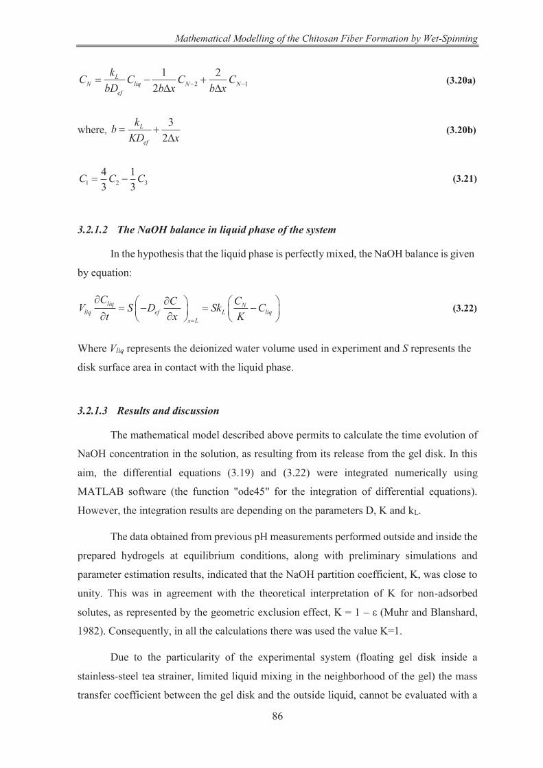
Mathematical Modelling of the Chitosan Fiber Formation by Wet-Spinning
86
2 11 2
2L
N liq N Nef
kC C C CbD b x b x
(3.20a)
where, 3
2L
ef
kbKD x
(3.20b)
1 2 34 13 3
C C C (3.21)
3.2.1.2 The NaOH balance in liquid phase of the system
In the hypothesis that the liquid phase is perfectly mixed, the NaOH balance is given
by equation:
liq Nliq ef L liq
x L
C CCV S D Sk Ct x K
(3.22)
Where Vliq represents the deionized water volume used in experiment and S represents the
disk surface area in contact with the liquid phase.
3.2.1.3 Results and discussion
The mathematical model described above permits to calculate the time evolution of
NaOH concentration in the solution, as resulting from its release from the gel disk. In this
aim, the differential equations (3.19) and (3.22) were integrated numerically using
MATLAB software (the function "ode45" for the integration of differential equations).
However, the integration results are depending on the parameters D, K and kL.
The data obtained from previous pH measurements performed outside and inside the
prepared hydrogels at equilibrium conditions, along with preliminary simulations and
parameter estimation results, indicated that the NaOH partition coefficient, K, was close to
unity. This was in agreement with the theoretical interpretation of K for non-adsorbed
solutes, as represented by the geometric exclusion effect, K = 1 – ε (Muhr and Blanshard,
1982). Consequently, in all the calculations there was used the value K=1.
Due to the particularity of the experimental system (floating gel disk inside a
stainless-steel tea strainer, limited liquid mixing in the neighborhood of the gel) the mass
transfer coefficient between the gel disk and the outside liquid, cannot be evaluated with a

Alin Alexandru ENACHE
87
reasonable reliability from the published correlations. However, the published correlations
could indicate, at least as the order of magnitude, its value. In the case we are investigating,
the mass transfer phenomenon is in some similarity with that occurring between a rotating
disk (with fixed spatial position) and a liquid. For this system it was proposed the correlation
(Cussler, 2007, Table 8.3-3):
1/2 1/30.62ReLk d ScD
;2
Re d; Sc
D (3.22)
d- dimeter of the disk;
D- NaOH diffusion coefficient in solution;
ω – rotation speed of the disk;
, - density and dynamic viscosity of the solution.
Considering the physical properties of the liquid water: =1000 kg/m3; =10-3 kg/(ms),
D=1.75∙10-9 m2/s (Farry, 1966) and ω =0.3 rot/s, one obtains: kL=2.2 10-5 m/s.
Another approximation of the diffusion coefficient can be obtained by its definition
in accord with the film theory:
LL
Dk , ( L- liquid film thickness) (3.23)
Considering a typical value for the liquid film thickness, L =0.1 mm=10-4 m (Cussler,
2007), one obtains: kL=1.75∙10-5 m/s.
The values of the effective NaOH diffusion coefficient in the gel, Def, could be
evaluated using the relations presented in Chapter 1. The difficulty in the use of these
relations comes from the unsteady-state character of the process (variation of NaOH
concentration in the system) and the lack of data regarding the dependence of NaOH
diffusion coefficient on the solution concentration. Nevertheless, for the diffusion
coefficient value given above, by using the relations (1.12). (1.13) and (1.14), there were
obtained the values presented in Table 3.1. Using these values of D, combined with the
approximated values for kL, in the simulation of the experiments described above, the
agreement between the calculated and experimental results was inadequate.

Mathematical Modelling of the Chitosan Fiber Formation by Wet-Spinning
88
Table 3.1. The diffusion coefficient value found by using the relations (1.12). (1.13) and (1.14). Chitosan concentration (wt. %) 1.0 1.5 2.0 2.5 3.0 3.5 4
Def ·10-9, m2·s-1
(1.12) 1.740 1.734 1.731 1.726 1.721 1.716 1.712
(1.13) 1.693 1.664 1.637 1.610 1.583 1.556 1.530
(1.14) 1.726 1.713 1.701 1.689 1.677 1.664 1.652
As no reliable data are available for the calculation of the parameters D and kL, their
values were estimated from the measured time evolutions of pH in the solutions outside the
gel samples, as explained in previous paragraphs. The estimation calculations were
performed by the least square method, using the "lsqcurvefit" function of MATLAB.
Considering the overall accuracy of the measurements and its averaging character,
we neglected the variation of mass transfer coefficient with the concentration of the
impregnating solution, using the same value of kL in all the estimations. The best estimated
value obtained in this way, was kL=1.85 10-5 m/s, which is in a rather good agreement with
the theoretical evaluations presented above. So, finally the values of the Def were estimated
using this value.
Examples of calculation results are given in Figures 3.5 and 3.6. Figure 3.5 presents
a comparison between the experimentally measured and calculated evolution of the NaOH
concentration outside the gel disk, using estimated parameters for D and kL. The time
evolutions of NaOH concentration inside the gel are presented in Figure 3.6. As expected,
due to the symmetry hypothesis, all the curves present a maximum in the center of the gel.
As observed from the Figure 3.6, the intensity of NaOH release is decreasing in time, due to
the decrease of the concentration gradient in the gel. So, the maximum NaOH concentration
decreased from 4 mol/L to ~2.3 mol/L (by 1.7 mol/L) in the first 147 s, whereas in the last
interval of time, a decrease from 2.3 mol/L to ~0.3 mol/L is achieved in 443 s.
The experiments were repeated with gels having different chitosan concentrations,
gels obtained by coagulation with different coagulant concentrations and gels impregnated
with NaOH solutions having different concentrations. In figures 3.7-3.10 are presented the
diffusion coefficient values estimated from data obtained by keeping constant each one of
these parameters.
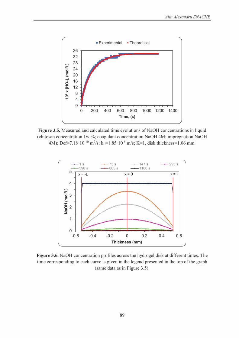
Alin Alexandru ENACHE
89
Figure 3.5. Measured and calculated time evolutions of NaOH concentrations in liquid (chitosan concentration 1wt%; coagulant concentration NaOH 4M; impregnation NaOH
4M); Def=7.18·10-10 m2/s; kL=1.85·10-5 m/s; K=1, disk thickness=1.06 mm.
Figure 3.6. NaOH concentration profiles across the hydrogel disk at different times. The time corresponding to each curve is given in the legend presented in the top of the graph
(same data as in Figure 3.5).
048
12162024283236
0 200 400 600 800 1000 1200 1400
104
x [H
O-],
(mol
/L)
Time, (s)
Experimental Theoretical
0
1
2
3
4
5
-0.6 -0.4 -0.2 0 0.2 0.4 0.6
NaO
H (m
ol/L
)
Thickness (mm)
1 s 73 s 147 s 295 s590 s 885 s 1180 s
x = 0x = -L x = L

Mathematical Modelling of the Chitosan Fiber Formation by Wet-Spinning
90
Figure 3.7. The calculated values of NaOH diffusion coefficient in hydrogels of disk shape, with different chitosan concentrations and different concentrations of the
impregnating NaOH solution (all hydrogels were prepared with NaOH 7M as coagulant).
Figure 3.8. The calculated values of NaOH diffusion coefficient in hydrogels of disk shape, with different chitosan concentrations, obtained with different concentrations of the coagulating NaOH solution (all hydrogels were impregnated with a NaOH solution 7M).
0.0
0.5
1.0
1.5
2.0
2.5
3.0
0 0.5 1 1.5 2 2.5 3 3.5 4
109
x D
ef, (
m2 /s
)
Cp (%)
1M NaOH impregnation 4M NaOH impregnation 7M NaOH impregnation
0.0
0.5
1.0
1.5
2.0
2.5
3.0
0 0.5 1 1.5 2 2.5 3 3.5 4
109
x D
ef, (
m2 /s
)
Cp (%)
1M NaOH coagulation 4M NaOH coagulation 7M NaOH coagulation
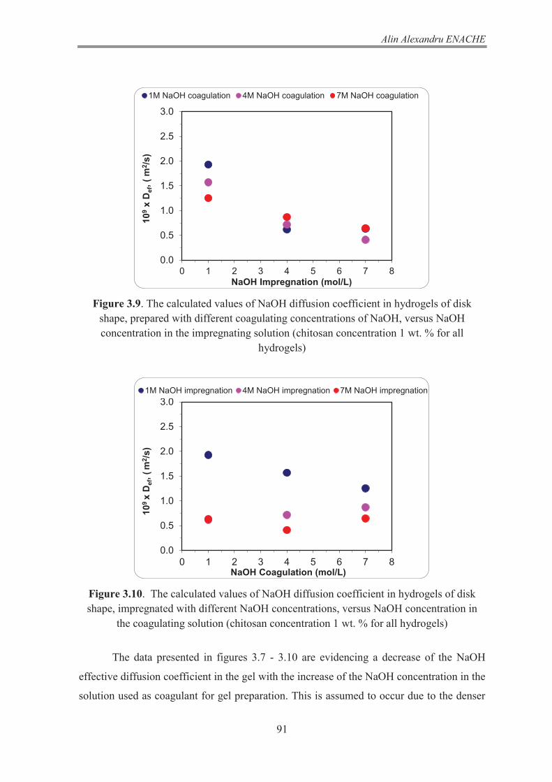
Alin Alexandru ENACHE
91
Figure 3.9. The calculated values of NaOH diffusion coefficient in hydrogels of disk shape, prepared with different coagulating concentrations of NaOH, versus NaOH concentration in the impregnating solution (chitosan concentration 1 wt. % for all
hydrogels)
Figure 3.10. The calculated values of NaOH diffusion coefficient in hydrogels of disk shape, impregnated with different NaOH concentrations, versus NaOH concentration in
the coagulating solution (chitosan concentration 1 wt. % for all hydrogels)
The data presented in figures 3.7 - 3.10 are evidencing a decrease of the NaOH
effective diffusion coefficient in the gel with the increase of the NaOH concentration in the
solution used as coagulant for gel preparation. This is assumed to occur due to the denser
0.0
0.5
1.0
1.5
2.0
2.5
3.0
0 1 2 3 4 5 6 7 8
109
x D
ef, (
m2 /s
)
NaOH Impregnation (mol/L)
1M NaOH coagulation 4M NaOH coagulation 7M NaOH coagulation
0.0
0.5
1.0
1.5
2.0
2.5
3.0
0 1 2 3 4 5 6 7 8
109
x D
ef, (
m2 /s
)
NaOH Coagulation (mol/L)
1M NaOH impregnation 4M NaOH impregnation 7M NaOH impregnation

Mathematical Modelling of the Chitosan Fiber Formation by Wet-Spinning
92
structure of the gel, formed at higher coagulant concentrations (see chapter 2). In the same
time, the diffusion coefficient is increasing with the decrease of the NaOH concentration in
the impregnating solution. Presumably, this is the effect of the increase of NaOH diffusivity
in aqueous solutions with the decrease of NaOH concentration (Farry, 1966). However, the
results presented in the first two figures do not evidence a clear dependence of the effective
diffusion coefficient in respect with the chitosan concentration in the gel. This suspicious
results could be explained by multiple factors: the experimental error in the measurement of
the pH, the unsteady character of the process, the limited mixing of the liquid, the non-
homogeneities occurring in the gel structure appearing during the coagulation process (see
chapter 2), the possible changes in the gel structure during the interval between their
preparation and their use in experiments, the errors in the measurement of disk thickness,
the changes in the NaOH concentration in the solution due to the absorption of carbon
dioxide from air etc.
3.2.2 Mathematical model of the NaOH release from hydrogels having infinite
cylinder geometry (radial diffusion)
The principle of determination of NaOH diffusion coefficient in hydrogels having
cylindrical shape is the same as in the hydrogel disk, the equation of diffusion (the second
law of Fick) being written for cylindrical geometry. So, both the experimental and
theoretical (modelling) treatment is very similar to the one described in the preceding
paragraph. However, the procedure is described completely without references to the
previous paragraph, in order to be easier followed and analyzed.
The following assumptions were used in order to characterize quantitatively the
sodium hydroxide diffusion process, during an experiment:
1. The process of sodium hydroxide transport inside the hydrogel cylinder is radial, the
axial diffusion is negligible (high length to radius ratio).
2. The flux is null in the center of cylinder.
3. An equilibrium state was established between the two phases at the hydrogel-liquid
interface (existence of a relation between the concentrations of sodium hydroxide in
the external liquid and chitosan hydrogel, on the interface).
4. Initially, the NaOH concentration is the same in all points of cylinder and it is equal
to the impregnating solution concentration.

Alin Alexandru ENACHE
93
As in the previous study, the mathematical model of the process will be obtained from
the NaOH balance equation in the gel sample and in external liquid respectively.
3.2.2.1 The NaOH balance in gel phase of the system
The only phenomenon occurring inside the hydrogel is an unsteady state sodium
hydroxide transport by diffusion. The space and time variations of NaOH concentration
inside the disk is given by the second law of Fick written in cylindrical coordinates:
11 efC CrDt r r r
(3.23)
where C - NaOH concentration inside the hydrogel, reported to the volume of inner liquid;
ε - polymer fraction inside the cylinder; Def is the effective diffusion coefficient.
The boundary conditions associated to the differential Equation 3.22 are involved at two
levels, at solution interface (r = R) and the center of the cylinder (r = 0).
A discontinuity is assumed on the gel interface between the equilibrium
concentrations of two phases (Ci(t) in liquid and C(R,t) in the gel), characterized by the
partition coefficient, K, and defined by the relation:
,
i
C R tK
C t (3.24)
A mass flux continuity is assumed on the gel-solution interface (r = R), expressed by
the following equation:
t > 0, r = R, ,
L i liq ef
C r tk C C D
r (3.25)
where kL is the mass transfer coefficient in the liquid phase film adjacent to gel interface.
The flux in the disk center is null and is described by the following equation:
t > 0, r = 0, ,
0C r t
r (3.26)
Initially (at the beginning of experiment), the sodium hydroxide concentration across
the hydrogel is constant:

Mathematical Modelling of the Chitosan Fiber Formation by Wet-Spinning
94
t = 0, 0 ≤ r ≤R ,0, 0 gelC r C (3.27)
If Def is constant during the process, the diffusion equation becomes:
2
211 ef
C C CD rt r r r
(3.28)
Further, the dimensionless radius was defined by the relation:
rR
(3.29)
By replacing, the equation (3.28) becomes:
2
2 211 ef
C C CDt R
(3.30)
The initial and in boundary conditions becomes:
t >0, ϕ=1, ,ef
L i liq
D C tk C C
R (3.31)
t >0, ϕ=0, ,
0C t
(3.32)
t=0, 0 ≤ ϕ ≤ 1, ,0, 0 gelC C (3.33)
The mass balance equation (3.29) was solved numerically, dividing the gel radius in
a number of N-1 uniform intervals, Δr (or ) i.e. N discretization points (Figure 3.11).
Using the notation j for a discretization point, with j = 1 corresponding to r = 0 or = 0
(cylinder center) and j = N to r = R or = 1 (the interface between hydrogel and liquid), the
spatial derivatives in the point j, can be approximated by the relations (3.34 and 3.35).
1 1
2j jC CC
(3.34)
21 1
22
2j j jC C CC (3.35)

Alin Alexandru ENACHE
95
Figure 3.11. Discretization of the chitosan hydrogel according to radius.
By replacing, the diffusion equation (3.30) becomes:
1 1 1 122
21
2j ef j j j j jC D C C C C C
t R (3.36)
Or equivalently,
1 122
11 2 4 22
j efj j j
C DC C C
t R (3.37)
By introducing the notations:
1 22
1 22 1
AR
(3.38)
2 22
21
AR
(3.39)
3 22
1 22 1
AR
, (3.40)
The differential equation (3.37) becomes
1 1 2 3 1( )jef j j j
CD AC A C A C
t (3.41)
This equation is written for all the spatial points between j = 2 and j = N-1,
obtaining (a system of N-2 differential equations in respect with the time. These can be used
to calculate the time variations of concentrations C2, C3…CN-1. The other two concentrations

Mathematical Modelling of the Chitosan Fiber Formation by Wet-Spinning
96
in j = 1 (C1) and j = N (CN) were obtained from the boundary conditions, in the same way as
for the diffusion in the disk. The derivative for =1 has the expression:
2 11
1 1 322 2N N N
C C C C (3.42)
By replacing (3.42) in the boundary equation (3.31), that becomes:
2 11 1 32
2 2efN
L liq N N N
DCk C C C CK R
(3.43)
Finally, it is found the recurrence relation of CN:
2 11 2
2L
N liq N Nef
kC C C CbD bR bR
(3.44)
32
L
ef
kbKD R
. (3.45)
The relation for the calculation of C1 was determined in the same way but using the
first three points (C1, C2 and C3):
1 2 30
1 3 42
C C C C (3.46)
At the center of the disk the flux is null, 0C
, so it is obtained:
1 2 34 13 3
C C C (3.47)
After all replacements, the balance of sodium hydroxide in solid phase is calculated
using the following mathematical model:
1 1 2 3 1j
ef j ef j ef j
CA D C A D C A D C
t, j=2,3…N-1 (3.48)

Alin Alexandru ENACHE
97
t > 0, ϕ = 0, 1 2 34 13 3
C C C
t > 0, ϕ = 1, 2 11 2
2L
N liq N Nef
kC C C CbD bR bR
(3.49)
t = 0, ,0,0 gelC C
3.2.2.2 The NaOH balance in liquid phase of the system
By assuming that the liquid phase is perfectly mixed, the NaOH balance is given by
equation:
1
liq N Nliq ef L liq
C C CV S D Sk Ct K
(3.50)
where Vliq represents the deionized volume water and S represents the external surface of
the cylinder.
3.2.2.3 Results and discussion
The mathematical model was solved using MATLAB software in the same way as
for the diffusion in the disk-shaped gels. The partition coefficient was taken K=1, from the
reasons presented in the preceding section. The mass transfer coefficient was calculated
using the equations presented in the paragraph 5.1.2 and its average value found was
1.85·10-5 m/s.
In Figures 3.12 and 3.13 are presented examples of calculated versus experimental
concentration evolutions in time and radial concentration profiles inside the gel
respectively. The process characteristics are similar with those evidenced in the analysis of
the diffusion in the disk geometry.
In Figures 3.14-3.17 are presented the values of the effective diffusion coefficient
determined at different concentrations of the impregnating solution, chitosan concentrations
in the gel and NaOH concentrations used for the gel preparation.
The values are delimited in the interval 10-9 to 1.310-9 m2/s. From the figures 3.14
and 3.15 is observed a slight decreasing trend of the diffusion coefficient with the increase

Mathematical Modelling of the Chitosan Fiber Formation by Wet-Spinning
98
of chitosan concentration, not observed in the case of disk geometry. The dependences in
respect with the NaOH concentrations in the coagulating solution and impregnating solution
respectively are less evident but seem to be present.
Figure 3.12. Experimental and calculated time evolutions of NaOH concentration in liquid for a hydrogel having infinite cylinder geometry; chitosan concentration 2.5 wt. %,
coagulated with NaOH 4M. The hydrogel was impregnated with NaOH 4M; Def=1.07·10-9 m2/s; kL=1.85·10-5 m/s; K=1.
Figure 3.13. Radial NaOH concentration profiles inside the hydrogel having infinite cylinder geometry; chitosan concentration 2.5 % coagulated with NaOH 4M. The hydrogel
was impregnated with NaOH 4M (same data as in Figure 3.12).
0.00
2.00
4.00
6.00
8.00
10.00
0 200 400 600 800 1000 1200 1400
10-4
x [H
O- ],
(mol
/L)
Time, (s)
Experimental Theoretical
00.5
11.5
22.5
33.5
44.5
5
-1.0 -0.8 -0.6 -0.4 -0.2 0.0 0.2 0.4 0.6 0.8 1.0
NaO
H, (
mol
/L)
Thickness, (mm)
1 s 73 s 146 s 293 s586 s 880 s 1173 s
r = 0r = -R r = R

Alin Alexandru ENACHE
99
Figure 3.14. The diffusion coefficient values for the sodium hydroxide through the chitosan hydrogels having infinite cylinder geometry at different chitosan concentrations
(Cp) impregnated with NaOH 7M. The legend indicates the coagulating NaOH concentrations.
Figure 3.15. The diffusion coefficient values for the sodium hydroxide through the chitosan hydrogels having infinite cylinder geometry, at different chitosan concentrations
(Cp) coagulated with NaOH 7M. The legend indicates the impregnating NaOH concentration.
0.8
1.0
1.2
1.4
1.6
0 0.5 1 1.5 2 2.5 3 3.5 4
109
x D
ef, (
m2 /s
)
Cp, (%)
1M NaOH coagulation 4M NaOH coagulation 7M NaOH coagulation
0.8
1.0
1.2
1.4
1.6
0 0.5 1 1.5 2 2.5 3 3.5 4
109
x D
ef, (
m2 /s
)
Cp, (%)
1M NaOH impregnation 4M NaOH impregnation 7M NaOH impregnation

Mathematical Modelling of the Chitosan Fiber Formation by Wet-Spinning
100
Figure 3.16. The diffusion coefficient values for the sodium hydroxide through the chitosan hydrogels having infinite cylinder geometry versus the concentration of
impregnating solution; chitosan concentration 2.5 wt. %. The legend indicates the NaOH concentration used in the coagulation.
Figure 3.17. The NaOH diffusion coefficient values through the chitosan hydrogels having infinite cylinder geometry versus the NaOH concentration used for coagulation; chitosan
concentration 2.5 wt. %. The legend indicates the NaOH concentration in the impregnating solution.
A comparison between the results obtained in the two set of experiments is
presented in the parity diagram, given in Fig. 3.18. The points in the diagram represent pairs
of diffusion coefficient values, obtained in identical working conditions, in the two types
of experiments.
0.8
1.0
1.2
1.4
1.6
0 1 2 3 4 5 6 7 8
109
x D
ef, (
m2 /s
)
NaOH Impregnation (mol/L)
1M NaOH coagulation 4M NaOH coagulation 7M NaOH coagulation
0.8
1.0
1.2
1.4
1.6
0 1 2 3 4 5 6 7 8
109
x D
ef, (
m2 /s
)
NaOH Coagulation (mol/L)
1M NaOH impregnation 4M NaOH impregnation 7M NaOH impregnation

Alin Alexandru ENACHE
101
Figure 3.18. Comparison between the averages values of Def in disk and in cylinder assuming K=1 and kL=1.85 x 10⁻⁵ m/s.
As observed from this figure, the dispersion of the results for the experiments
conducted in the disk geometry is very important, much higher than those obtained from
cylindrical geometry. So, the values determined from the experiments with cylindrical
samples seem to be more reliable. The points in figure, are grouped in the three sets,
according to the magnitude and sign of the differences. The group (a) includes the points
representing diffusion coefficients smaller for disk geometry, whereas the group (b)
contains the points representing values higher for disk geometry. The group (c) includes the
points placed furthest from the first bisector, i.e. the points indicating the biggest
differences. The rather high values of the effective diffusion coefficient measured for the
disk geometry in this group, higher than those reported for the diffusion coefficient in
solution, make them less reliable. Therefore, we can consider that the most reliable values
are in the groups (a) and (b), including the higher number of points. From these two groups
it can be inferred an overall averaged value for the NaOH diffusion coefficient in chitosan
gels, determined in the working conditions, of 1.2 10-9 m2/s.
Unfortunately, the experimental results obtained do not permit a systematic and
general valid conclusion concerning the dependences of the diffusion coefficient on the
concentration of chitosan in the gel and on the concentration of NaOH in the solutions used
for coagulation or for impregnation. The sources of errors are presented in the previous
section. Therefore, other more accurate method should be applied, in order to obtain more
reliable information regarding the values of the effective diffusion coefficient and its
0.00
0.50
1.00
1.50
2.00
2.50
3.00
0.00 0.50 1.00 1.50 2.00 2.50 3.00
109
x D
disk
(109
m2 /s
)
109 x Dcylinder (m2/s)
1M - 1M
1M - 4M
1M - 7M
4M - 1M
4M - 4M
4M - 7M
7M - 1M
7M - 4M
7M - 7M
(b)
(a)
(c)

Mathematical Modelling of the Chitosan Fiber Formation by Wet-Spinning
102
dependence on the gel characteristics. In the next two chapters are presented the
experimental studies and theoretical calculations based on the coagulation experiments,
eliminating some of the sources of errors appearing in the presented study.
Alin Alexandru ENACHE
103
STUDY OF THE CHITOSAN
COAGULATION KINETICS BY EXPERIMENTS
IMPLYING LINEAR DIFFUSION

Mathematical Modelling of the Chitosan Fiber Formation by Wet-Spinning
104
Introduction
The objectives of this chapter are to investigate the kinetics of chitosan hydrogels
formation from aqueous chitosan solutions, using sodium hydroxide (NaOH) as coagulant
and simultaneously to determine the values of NaOH diffusion coefficient in chitosan gels,
by a more accurate method, as compared with that presented in previous chapter. The
experiments were performed in a transparent parallelepiped shaped cell that implies
unidirectional chitosan coagulation and NaOH diffusion. As mentioned in the previous
chapters, the coagulation occurs by neutralization of protonated amino groups (–NH3+)
present in the solubilized chitosan chains, the kinetics being controlled by NaOH transport
towards the coagulation zone. The study confirmed the appropriateness of Fick’s second law
to describe the NaOH transport, considering instantaneous reaction between the NaOH and
-NH3+ groups. The experimental data were used to determine the NaOH diffusion coefficient
in gels having different chitosan concentrations.
4.1 Materials and Methods
The materials used and the preparation of the chitosan solution (i.e. collodions or
dopes) are described in the paragraph 2.3. The coagulation experiments were performed with
chitosan solutions having the concentrations ranging between 1 % and 4% (wt.) and sodium
hydroxide solutions with concentrations between 1M and 7M, as coagulation agent.
The coagulation experiments were performed in a transparent quartz cell (volume 350
μL) manufactured by Hellma Analytics (type 100 QS/100-1-40), having the outer
dimensions 45x12.5x3.5 mm, light path of 1 mm and inner width 9.5 mm. This was carefully
filled with chitosan solution and was immobilized (by a double-sided tape) on the bottom of
a Petri dish (100 mm in diameter), filled thereafter with a volume of 80 mL aqueous solution
of NaOH. The kinetics of coagulation was investigated by measuring the time evolution of
the hydrogel volume inside the transparent cell. In this aim, there were registered images of
the hydrogel layer, at different coagulation times, by an optical microscope Olympus BX41
(4x objective), coupled with an Olympus DP26 camera, connected on-line to a PC, using
Olympus cellSens software (Figure 4.1). All the experiments were conducted at room
temperature (25 oC).

Alin Alexandru ENACHE
105
Figure 4.1. Image of the experimental setup for the study of linear coagulation kinetics.
The aqueous NaOH solution was not stirred, due to technical difficulties (lack of
space, due to the volume occupied by the microscope).
The time evolution of the hydrogel layer thickness, inside the cell, was obtained from
the images registered at different coagulation times. In what follows, the interface between
the NaOH aqueous solution and the chitosan hydrogel will be named front interface, whereas
the interface between the gel and the chitosan solution will be referred to as coagulation
interface (Figure 4.2). Also, the terms hydrogel and gel will be used interchangeably.
4.2 Mathematical model of the coagulation process
In order to build a mathematical model of the coagulation process, we adopted the
following hypotheses:
- the reaction between the -NH3+ moieties and NaOH is much faster than the NaOH effective
diffusion through the gel, so it will be considered instantaneous (Knaul, 1997). This
assumption is supported by the distinct boundary observed experimentally between the
hydrogel and the chitosan solution;
- the transport of NaOH through the hydrogel occurs only by diffusion, in a single direction,
along the cell axis (perpendicular to the hydrogel/dope interface) or in radial direction (in
the cylinder geometry experiments);
- NaOH diffusion coefficient is constant across the chitosan hydrogel and in time;

Mathematical Modelling of the Chitosan Fiber Formation by Wet-Spinning
106
- NaOH concentration in the aqueous solution outside the gel is considered constant during
coagulation, due to the large excess of NaOH;
- on the front interface there is fulfilled the condition of NaOH flux continuity;
- NaOH concentration at the hydrogel/dope interface (coagulation interface) is negligible
small, with a fast pH variation across the coagulation interface (Venault et al., 2012).
Figure 4.2. Representation of the coagulation system in coagulation/optical cell with
notations for the coagulation interface location and concentrations in the different boundaries
According to these hypotheses, the overall process kinetics is controlled by the
transport of NaOH from the aqueous solution toward the coagulation zone.
The NaOH balance equation inside the chitosan hydrogel (second Fick’s law) has
the general form:
2
21 efC CDt x
(4.1)
where C is the NaOH concentration in the hydrogel. The variable x represents the transport
coordinate, having the origin on the front interface.
The left-hand side term of equation (4.1) represents the overall NaOH accumulation
in the assessable unit volume of chitosan gel, as result of diffusion, the only mechanism of
mass transport considered inside the gel.

Alin Alexandru ENACHE
107
The initial and boundary conditions associated to Equation (4.1) are (see Figure 4.2):
i) The condition of NaOH absence in the dope at the initial time (t=0):
t = 0, 0 ≤ x ≤ L, , 0 0C x (4.2)
ii) The NaOH flux continuity on the front interface, i.e. the equality between the flux
transferred from the bulk liquid NaOH solution toward gel surface and the flux diffusing
from the surface, through the gel.
According to Cussler (1997), the NaOH flux from the bulk liquid NaOH solution
toward gel surface can be expressed alternatively, by using diffusion coefficients or mass
transfer coefficients. However, when the diffusion occurs across an interface, it is
customarily to use mass transfer coefficient approach. According to this recommendation,
on the front interface we used the boundary condition:
x = 0, t > 0, L sol i efCk C C Dx
(4.3)
where Csol is the NaOH concentration in the bulk aqueous solution and Ci is the NaOH
concentration in the aqueous solution at the front interface. In this approach, the liquid phase
resistance to NaOH transport is expressed quantitatively by the inverse of the mass transfer
coefficient, kL.
iii) The condition of null NaOH concentration at the coagulation interface (the consumption
of NaOH is much faster than its transport by diffusion) or null NaOH flux, when coagulation
is completed:
x = δ < L, t > 0, , 0C t (4.4a)
x = δ = L, t > 0, 0Cx
(4.4b)
The time evolution of hydrogel thickness is calculated considering the stoichiometric
relation existing between the molar fluxes of NaOH and –NH3+ groups consumed on the
coagulation interface (x= ), defined by the equation:
x = δ, t > 0, 3
,ef NH
C tD C
x t (4.5a)
or:

Mathematical Modelling of the Chitosan Fiber Formation by Wet-Spinning
108
3
,ef
NH
D C tt C x
(4.5b)
The model defined above was solved numerically by the method of lines, presented in
Chapter 3. To this aim, the x axis (inner cell length) of initial chitosan solution was divided
into N-1 intervals, of width x. The spatial derivative, appearing in equation (4.1), was
approximated by finite differences and following the procedures presented in the previous
chapter, one obtains the system of ordinary differential equations:
1 12 21
j efj j j
C DC C C
t x, j=2,…N-1 (4.6)
In these equations, Cj represents the NaOH concentration at point xj=(j-1)· x. The time
evolutions of the concentrations Cj in the discretization points have been calculated by
numerical integration of equations system (4.6), simultaneously with the Equation (4.5b),
describing the evolution of hydrogel thickness. The integration was performed by using the
‘ode45’ function of the Matlab® scientific package. On the hydrogel front interface, it is
assumed an equilibrium state between the NaOH concentrations in the two phases, i.e. in the
liquid at the surface of the gel (Ci) and within the gel at x=0, where the NaOH concentration
is C(0,t)=C1. This equilibrium is characterized by the partition coefficient, K, defined by the
relation:
10,
i i
C t CKC C
(4.7)
The concentration gradients, ∂C(0,t)/∂x and ∂C( ,t)/∂x appearing in the boundary
condition (4.3) and equations (4.5), were calculated from the second order polynomial
interpolations of the concentration variations with spatial coordinate x, using the calculated
values of C for several discretization points in the neighborhoods of x=0 and x=
respectively.
A difficulty in the numerical integration of these equations resides in the
initialization of the concentration profile inside the hydrogel (obtaining an initial NaOH
concentration profile in a given hydrogel thickness, formed in a known coagulation time).
The adopted procedure is based on the hypothesis that NaOH concentration inside the
hydrogel at the (front) interface with the NaOH solution (C1) is constant over a rather short

Alin Alexandru ENACHE
109
time interval (5 - 10 s), at the beginning of the coagulation process. For a constant NaOH
concentration on the hydrogel surface, the Equation (4.1) has the analytical solution given
by expression (4.8) (Paul, 1968; Liu et al., 1989).
1
2, 1
2
ef
ef
xerfD t
C x t C
erfD t
, 0
2 yerf y e d (4.8)
By calculating the NaOH concentration gradient at the hydrogel/chitosan solution
interface, from expression (4.8), and substituting in (4.5b), one obtains the time variation of
the hydrogel thickness:
3
2
1 exp4
2
efef
NHef
ef
CD tD
t CD t erf
D t
(4.9)
Once an initializing profile was obtained from equations (4.8) and (4.9), the process
evolution was calculated by numerical integration of equations (4.5b) and (4.6), considering
the time variation of NaOH concentration C1(t) at the interface between the gel and NaOH
solution.
4.3 Results and discussion
4.3.1 Experimental results
As already described, the chitosan coagulation mechanism involves the reaction of
the protonated amino -groups (-NH3+), of the dissolved chitosan macromolecules, with
hydroxyl ions (HO-) of coagulant, conducting to the neutralization of chitosan chains. This
in turn favors macromolecular interactions (hydrogen bonds, hydrophobic interactions,
crystallites and entrapped entanglements), giving rise to the hydrogel layer. Further, the
sodium hydroxide is diffusing through the chitosan hydrogel so formed, toward the
hydrogel-chitosan dope interface, continuing to neutralize and to increase the hydrogel
stratum thickness.

Mathematical Modelling of the Chitosan Fiber Formation by Wet-Spinning
110
The coagulation experiments were performed with chitosan solutions having the
concentrations between 1 wt. % and 3.9 wt. % (corresponding to concentrations of the
repeating unit of polymer, between 60 and 240 mol/m3) and sodium hydroxide solutions 1M
and 7M. As mentioned, no significant swelling or syneresis effects were observed during
the experiments, the gel volume being the same with the volume of gelated chitosan solution.
Figure 4.3 presents a snapshot of the hydrogel layer between the two solutions,
during the experiment. As can be observed from this figure, the hydrogel and the chitosan
dope are separated by a distinct boundary (also observed by Rivas Araiza et al., 2010),
indicating a very tinny reaction zone of NaOH with solubilized chitosan molecules,
consequence of the fast-ionic reaction.
Another feature observed from Figure 4.3 is a nonhomogeneous morphology of the
hydrogel. This presents a homogeneous zone only in the proximity of the front interface and
a fascicle of capillaries, closer the coagulation interface. The formation of this capillary
fascicle is explained by the high concentration gradients appearing at the proximity of
coagulation front and the local hydrodynamic phenomena induced by the collapse of
chitosan chains from the solution to the gel (Rivas Araiza et al., 2010; Sereni et al., 2017).
The coagulant diffusion throughout the two structural zones of the gel is
characterized by different resistances and consequently different diffusion intensities.
Therefore, the diffusion coefficient value, inferred from experimental data, is an ‘effective’
or ‘apparent’ one, representing an average over the whole structure of the gel. The measured
evolutions of hydrogel thickness with coagulation time, for chitosan solutions of different
concentrations, are presented in Figure 4.4 and Figure 4.5 for NaOH concentrations 1M and
7M respectively. As expected, the increase of the gel thickness is faster on the first part of
coagulation process, due to the smaller diffusion distance of coagulant between the front
interface and the coagulation interface. At longer gelation times, the transport distance inside
the gel is larger and the growth rate of the hydrogel is decreasing, becoming almost constant
at the end of the coagulation process, where the curves have approximately linear shapes.

Alin Alexandru ENACHE
111
Figure 4.3. A snapshot of the coagulation process.
As seen from the Figures 4.4 and Figure 4.5, the rate of chitosan coagulation from
its aqueous solutions (defined here as the speed of coagulation front) increases with the
decrease of chitosan concentration and the increase of coagulation agent concentration.
The decrease of the coagulation front speed with the increase of chitosan
concentration is explained by the increased number of -NH3+ moieties to be neutralized,
combined with a slightly higher resistance opposed by solid phase to coagulant diffusion
(lower value of NaOH diffusion coefficient in the gel). However, the dependence of
coagulation front speed on chitosan concentration is not linear.
At a given coagulation agent concentration and coagulation time, the ratio of the gel
thicknesses obtained for two chitosan concentrations is smaller than the reversed chitosan
concentrations ratio.
As an example, consider the gels thicknesses calculated for a coagulation time of
2000 s, as resulting from Figure 4.4. The gel thickness is 5.8 mm for the chitosan solution 1
% and 4 mm for the chitosan solution 3.9 %. Even if the NaOH diffusion coefficient values
in the two gels are comparable, the gel thicknesses ratio is around 1.45 for a ratio of chitosan
concentrations around 4. The explanation resides in the increase of NaOH concentration
gradient in the gel with chitosan concentration, i.e. a steeper decrease of NaOH
concentration in a more concentrated gel, due to a higher density of neutralized -NH3+
groups. This is inducing an acceleration of the diffusion, leading to a higher NaOH flux on
the coagulation interface (Figure 4.6). A similar conclusion can be drawn regarding the
influence of coagulant concentration on the gel thickness. As can be observed from Figure

Mathematical Modelling of the Chitosan Fiber Formation by Wet-Spinning
112
4.4 and Figure 4.5, for a chitosan concentration of 1 %, by increasing the coagulant
concentration from 1M to 7M the gel thickness obtained in 3600 s is increasing from 7.8
mm to 9.6 mm. So, a seven-fold increase of NaOH concentration leads to only a 1.24-fold
increase of gel thickness.
Figure 4.4. Measured and calculated hydrogel thickness versus gelation time, for different chitosan concentrations; symbols- measured values; solid lines- calculated values (NaOH
solution 1M). The legend gives the polymer concentration of the solutions (in wt. %).
Figure 4.5. Measured and calculated hydrogel thickness versus gelation time, for different chitosan concentrations; symbols- measured values; solid lines- calculated values (NaOH
solution 7 M). The legend gives the polymer concentration of the solutions (in wt. %).
0
1
2
3
4
5
6
7
8
0 1000 2000 3000 4000
Thick
ness
(mm
)
Gelation Time (s)
1% 1.5% 2% 2.5% 2.8% 3.5% 3.9%
0123456789
10
0 1000 2000 3000 4000
Thic
knes
s (m
m)
Gelation Time (s)
1% 1.5% 2% 2.5% 2.8% 3.5% 3.9%

Alin Alexandru ENACHE
113
Figure 4.6. Time evolutions of NaOH flux on the coagulation interface (N( ,t)).
In order to evidence the explanation of this result, we consider the mass balance of
NaOH during the coagulation time, tc, defined by the equation:
mf = ma + mr (4.10)
30 0 0
0, ; , ; ,c ct t
f a c r NHm S N t dt m S C x t dx m S N t dt S C (4.11)
where mf, ma and mr are the the amounts of NaOH fed into the gel, accumulated into the gel
and neutralized respectively.
The NaOH quantity consumed in the coagulation process, mr, is depending on the
NaOH flux at the coagulation front, N( ,t), which is decreasing in time, due to the increase
of resistance opposed to the NaOH transport (Figure 4.6). Similarly, the fed quantity of
NaOH into the gel, mf, is depending on the input flux at the front interface, N(0,t), which is
decreasing with time, due to the decrease of concentration gradient on the front interface, as
result of NaOH accumulation into the gel (Figure 4.7). The effect of NaOH concentration
growth from 1M to 7M, keeping the chitosan concentration constant at 1 %, is a significant
increase of mass flux on the front interface and a less important increase of the flux on the
coagulation interface (Figure 4.6 and Figure 4.7).

Mathematical Modelling of the Chitosan Fiber Formation by Wet-Spinning
114
Figure 4.7. Time evolutions of NaOH flux on the front interface (N(0,t)).
The flux on the coagulation interface, when using NaOH solution 7M, is only slightly
superior to that corresponding to the solution 1M (Figure 4.6), thus explaining the value of
gel thickness, not very different of that obtained with the coagulant concentration 1M.
Nevertheless, the amount of NaOH accumulated inside the gel is superior to the
amount consumed in the coagulation reaction, the ratio between the two quantities rising
with the NaOH concentration in the solution used for coagulation.
4.3.2 Simulation of the linear coagulation
The numerical solution of the coagulation process model was calculated by the
procedure described previously. The integration was initialized by using an approximate
solution defined by relations (4.8) and (4.9), for a duration of 5 to 10 s.
The main parameters of the coagulation process model defined above are the NaOH
diffusion coefficient inside the chitosan hydrogel, Def, the liquid-solid (hydrogel) NaOH
mass transfer coefficient at the front surface, kL, and the partition coefficient K.
Our preliminary parameter estimations, including K as an unknown parameter,
together with pH measurements performed in immerged NaOH aqueous solutions inside
the prepared hydrogels, indicated that the NaOH partition coefficient between NaOH
solution and chitosan hydrogel was close to unity. This is in agreement with the theoretical
interpretation of the partition coefficient for non-adsorbed solutes (in the hypothesis of

Alin Alexandru ENACHE
115
weak interactions between Na+, HO- and chitosan), as representing the geometric exclusion
effect, K=1-ε (Muhr et Blanchard, 1982). This corresponds, in our working conditions, to
values of K between 0.96 and 0.99.
The influence of the partition coefficient, K, on the calculated time evolution of gel
thickness is presented in Figure 4.8. This diagram shows that, on the domain 0.95 - 1, the
value of K does not influence significantly the time evolution of gel thickness.
Consequently, in this study we fixed the value K=1.
In preliminary simulations we tested the values of NaOH diffusion coefficient in the
gel (Def), calculated from the relations (1.12), (1.13) and (1.14), using estimated or published
values for the diffusion coefficient in the solution (D), as will be described below. However,
the results were significantly different from experimental observations (significant errors in
the calculation of gel thickness).
Figure 4.8. Influence of the partition coefficient, K, on the calculated time evolution of gel
thickness (1 % chitosan; NaOH solution 7M; Def=1.65·10-9 m2∙s-1; kL=7.5·10-6 m·s-1).
Similarly, as pointed up by different authors, no general and reliable data are available for
the calculation of liquid-solid mass transfer for limiting cases of slow flow or stagnant
liquids (Bird et al., 2002).
Therefore, we used a fitting procedure to determine the values of both kL and Def,
based on the experimental measurements presented above. The value of the volume fraction
of chitosan in the hydrogel, was calculated from the chitosan mass fraction, w, by the
relation:

Mathematical Modelling of the Chitosan Fiber Formation by Wet-Spinning
116
1
1 2
// /
ww w
(4.12)
It was approximated by the chitosan volume fraction in the dope, since no syneresis
could be evidenced at the walls of the diffusion cell.
By applying the least square method, we obtained the value of the mass transfer
coefficient, kL=7.5∙10-6 m·s-1 and the values of Def presented in Table 4.1, dependent on the
chitosan and NaOH concentrations. Our calculations indicated that the influence of kL on
the gel thickness is weaker than the influence of Def; therefore, we used the same value of
kL for both NaOH solutions.
The estimated diffusion coefficient values, presented in Table 4.1, are indicating a
significant decrease of sodium hydroxide diffusivity in the hydrogel, with the increase of
chitosan concentration, most probably due to an increased resistance induced by an
increased “solid” volume fraction. In the same time, it can be observed a decrease of the
diffusion coefficient with the increase of sodium hydroxide concentration from 1M to 7M,
possibly due to the increase of solution viscosity and the impact of neutralization conditions
on the morphology of the gels and their diffusive resistance. These values are higher than
the one estimated by Rivas Araiza et al. (2010), Def =0.4∙10-9 m2/s, for a gel obtained from
a dope solution containing 5 % (wt.) chitosan. This difference could be explained by a higher
chitosan concentration in the gel (inducing a higher resistance to diffusion) and the disregard
of the external resistance (to the liquid-gel transfer) in the calculation of Rivas Araiza et al.
(2010) (thus the reported value of Def is including also the external resistance).
Table 4.1. Estimated diffusion coefficient values (kL =7.5∙10-6 m·s-1).
Chitosan concentration, (wt. %)
1 1.4 2 2.5 2.8 3.3 3.9
Def ∙109, m2·s-1 1M 1.80 1.75 1.70 1.65 1.55 1.50 1.45
7M 1.65 1.60 1.55 1.50 1.45 1.40 1.35
The value of diffusion coefficient of NaOH in dilute aqueous solutions can be
estimated by averaging the diffusivities of the ions Na+ and HO- (DNa+ and DHO-). Using the
ions diffusivities and the averaging formula published by Cussler (1997).
1 2 2 1
1 2
z z z zD D D
(4.13)

Alin Alexandru ENACHE
117
where D1= DNa+=1.33∙10-9 m2·s-1; D2= DHO- =5.28∙10-9 m2·s-1, z1=+1 and z2 =-1, one
obtains the NaOH diffusion coefficient, D=2.125 ∙10-9 m2·s-1. Similar values of NaOH
diffusion coefficient in aqueous solutions were published by Fary (1996). For a NaOH
concentration of 1M, at room temperature, this author reports a value D=1.75∙10-9 m2·s-1.
The values of NaOH diffusion coefficients in the two solutions, 1M and 7M
respectively, free of chitosan, can be predicted by graphical extrapolation. Constructing the
graphs diffusion coefficient - chitosan concentration and extrapolating to null chitosan
concentration, there are obtained the values 1.9∙10-9 m2∙s-1 for the solution 1M and 1.76∙10-
9 m2∙s-1 for the 7M solution (Figure 4.9). The value of the NaOH diffusion coefficient in the
solution 1M is enclosed in the interval between that reported by Fary (1996) and the one
estimated by the relation (4.13). A decrease of the diffusion coefficient with the increase of
NaOH concentration in aqueous solutions was also reported by Fary (1996).
In Figure 4.10 is presented a comparison between the values of diffusion coefficients
calculated by relations (1.14), (1.12) and (1.13) presented in Chapter 1, and those estimated
from experimental data, for coagulant solution 1M.
Figure 4.9. Graphical extrapolations for NaOH diffusion coefficient.
In the relation (1.14) we used the value α=1.67 and in relation (1.13) we approximated ’= .
As can be observed, the prediction error increases with the chitosan concentration in the gel.
The diffusion coefficient values calculated by relation (1.12) proved to be the closest
to experimental data. The average error for the relation (1.12) is 8.02 % for the data obtained
with the NaOH solution 1M and 8.53 % for the data obtained with the solution 7M. The
0 1 2 3 41,3
1,4
1,5
1,6
1,7
1,8
1,9
2,0
Def (1
09 m2 /s
)
Cp (%)
1M 7M

Mathematical Modelling of the Chitosan Fiber Formation by Wet-Spinning
118
average error associated with the other relations are around 13.5 % for relation (1.14) and
around 16 % for the relation (1.13).
Figure 4.10. Comparison between the predicted values of NaOH diffusion coefficient in chitosan gel using relations (1.14 noted Rel (1) in graph), (1.12, noted Rel (2) in graph)
and (1.13, noted Rel (3) in graph) presented in Chapter 1, and the measured values using the diffusion cell.
In order to check also the reliability of the estimated value of kL, we appraised it
theoretically by several models published in chemical engineering literature. They use the
dimensionless numbers Sherwood (Sh) (the ratio between the rate of convective mass
transfer through the liquid film to the rate of diffusive mass transport in the liquid) and Biot
(Bi) (the ratio between the rate of convective mass transfer through the liquid film to the rate
of diffusive mass transport inside the gel). Different authors identified asymptotic values for
Sh number, characterizing the mass transfer between a solid particle and a surrounding fluid
with small or null velocity. A classical value frequently reported for a spherical particle is
Sh = 2. A limiting value Sh = 4 was also found theoretically for regular packing, if based on
the local difference between interfacial and bulk concentrations (Bird et al., 2002).
Besides, there are reported values for the Bi number characterizing the mass transfer
between stagnant liquid zones and solid porous particles in packed beds. Iliuta et al. (1999)
found, by tracer experiments, Bi values between 1 and 11. In the expression of Sh and Bi
numbers we used the equivalent diameter, defined as the diameter of a sphere having the
same external surface area (S) as the active (open) surface area of the coagulation cell:
pd

Alin Alexandru ENACHE
119
;
2
L p L p
ef
p p
k d k rSh Bi
D D
Sd r
(4.14)
Using the cell dimensions of the cell used in our experiments, Sh = 2 and
D = 1.83∙10-9 m2·s-1 (an average value), one obtains a mass transfer coefficient value,
kL = 2.1∙10-6 m·s-1. On the other side, the values of Bi between 1 and 11 lead to values of kL
between 1.6∙10-6 m·s-1 and 2.33∙10-5 m·s-1. Therefore, we appreciate that the value
kL = 7.5∙10-6 m·s-1 is well estimated within the published data ranges.
The comparisons between the calculated and experimental hydrogel thickness
values, presented in Figure 4.4 and Figure 4.5, are evidencing a good phenomenological
quality of the modeling approach, which, along with the reliability of mass transport
parameters values, are demonstrating the suitability of the proposed mathematical model.
Typical NaOH concentration profiles inside the hydrogel, calculated at different coagulation
times are given in Figure 4.11. As can be observed, the NaOH concentration at the front
interface is not constant, presenting an increasing evolution in time.
Figure 4.11. NaOH concentration profiles inside the hydrogel (1 wt. % chitosan and 7M NaOH).
This is the result of the increase of gel resistance to the NaOH transport toward the
coagulation interface, due to the increase of gel thickness. The growing resistance of the gel
stratus is inducing a decrease of NaOH flux and an increased NaOH concentration in the gel
volume, i.e. a decreasing concentration gradient and an increasing interface concentration
(see relation (4.3)).

Mathematical Modelling of the Chitosan Fiber Formation by Wet-Spinning
120
EXPERIMENTAL AND MODELING
STUDY OF THE COAGULATION STEP IN THE
CHITOSAN WET-SPINNING PROCESS

Alin Alexandru ENACHE
121
Introduction
This chapter presents the studies of the chitosan fiber formation process by wet
spinning of the chitosan acid solution. There were performed experimental studies aiming
to determine the NaOH diffusion coefficient in cylindrical coagulation (radial diffusion of
coagulant) and chitosan wet spinning experiments on a laboratory scale unit. The
experimental results were used in a theoretical study aimed to develop a mathematical model
useful in the analysis and design calculations of the wet-spinning process. As shown in the
previous chapter, the main parameter of the coagulation model is the coagulant diffusion
coefficient in the gel. The published studies are evidencing differences between the diffusion
coefficient’s values calculated from linear diffusion experiments, as compared with radial
diffusion. Consequently, a first study presented in this chapter regards the determination of
the NaOH diffusion coefficient in chitosan gel samples having cylindrical geometry. The
diffusion coefficient values so obtained were used in the wet spinning process modelling
and simulations study, described in the second part of this chapter.
5.1 Study of the chitosan coagulation kinetics by experiments with radial
diffusion
5.1.1 Experimental study
5.1.1.1 Method
The materials used and the preparation of the chitosan solution are described in the
paragraph 2.3. The coagulation experiments were performed with chitosan solutions having
the concentrations between 2% and 4% w/w and sodium hydroxide solutions 1M, 4M and
7M.
In order to investigate experimentally the coagulating kinetics of chitosan solution
(dope) having cylindrical shape (radial diffusion of sodium hydroxide), the chitosan dope
samples having cylindrical geometry (filaments) were exposed to coagulating times between
15 s and 5 minutes, keeping constant the working conditions (the same chitosan
concentration, temperature and NaOH concentration in the coagulating bath). After a given
coagulation time, the chitosan gel tube was removed from the coagulation bath, wiped with
filter paper and cut at both ends. Further, the non-coagulated chitosan solution was removed
by using compressed air and finally, the tube was sampled in small pieces and passed to

Mathematical Modelling of the Chitosan Fiber Formation by Wet-Spinning
122
microscopy, where the thickness of coagulated chitosan membrane so obtained was
measured (Figure 5.1). The microscope used was a Leica M205A stereo.
Figure 5.1. The process diagram: (1) coagulated bath; (2, 3) removing the non-coagulated
chitosan; (4) cutting the samples; (5) taking the images by using a microscope; (6) measuring the thickness of the coagulated chitosan.
5.1.1.2 Experimental results
In Figure 5.2 is presented a sequence of registered images, illustrating the progress
of chitosan hydrogel thickness as a function of coagulation time.
The measured time evolutions of gel thickness, working with chitosan solutions of
different concentrations, are presented in Figures 5.3 to 5.5, for sodium hydroxide
concentrations 1M, 4M and 7M respectively. As seen from these figures, the rate of chitosan
coagulation from its aqueous solutions (the speed of coagulation front displacement)
increases with the decrease of chitosan concentration, and the increase of coagulation agent
concentration. The explanation of this result stems in the diffusion control of the coagulation
kinetics and a higher solid volume fraction of the gels formed from more concentrated
chitosan solutions, inducing a stronger hindrance to the sodium hydroxide transport by
diffusion.

Alin Alexandru ENACHE
123
Figure 5.2. The propagation of the gel front for 2% (w/w) chitosan coagulated with 7M NaOH: a) 60 s; b) 120 s; c) 180 s; d) 240 s; e) 300 s.
Figure 5.3. Measured and calculated increase of hydrogel thickness as a function of
gelation time for different chitosan concentrations; points - measured values; solid lines - calculated values (NaOH solution 1M). The legend gives the polymer concentration (in wt.
%).
0.00
0.50
1.00
1.50
2.00
0 100 200 300 400
Thic
knes
s (m
m)
Gelation Time (s)
2% 2.5% 3% 3.5% 4%

Mathematical Modelling of the Chitosan Fiber Formation by Wet-Spinning
124
Figure 5.4. Measured and calculated increase of hydrogel thickness as a function of
gelation time (for different chitosan concentrations; symbols - measured values; solid lines - calculated values (NaOH solution 4M). The legend gives the polymer concentration (in
wt. %).
Figure 5.5. Measured and calculated increase of hydrogel thickness as a function of
gelation time for different chitosan concentrations; symbols-measured values; solid lines- calculated values (NaOH solution 7M). The legend gives the polymer concentration (in wt.
%).
0.00
0.50
1.00
1.50
2.00
0 100 200 300 400
Thic
knes
s (m
m)
Gelation Time (s)
2%1M exp 2.5 % EXP 3% EXP 3.5% exp 4% exp
0.00
0.50
1.00
1.50
2.00
2.50
0 100 200 300 400
Thic
knes
s (m
m)
Gelation Time (s)
2%1M exp 2.5 % EXP 3% EXP 3.5% exp 4% exp

Alin Alexandru ENACHE
125
5.1.2 Modeling of the chitosan coagulation process in cylindrical geometry
5.1.2.1 Mathematical model
In order to obtain a mathematical model of the coagulation process, the following
hypothesis were adopted:
the neutralization reaction between the groups and NaOH is instantaneous
(Knaul, 1997), so that the step controlling the coagulation kinetics is the diffusion of
NaOH trough the gel;
the NaOH concentration at the gel / chitosan solution interface is negligible small;
the concentration of sodium hydroxide inside the chitosan solution is null;
the NaOH concentration in coagulation solution is approximated constant in time.
This hypothesis is supported by the very high excess of NaOH into the aqueous
solution;
the NaOH diffusion coefficient is constant inside chitosan hydrogel.
Figure 5.6. The chitosan gel formation in cylindrical geometry coagulation
The sodium hydroxide balance inside the chitosan gel is given by Fick’s second law
expression:
3NH

Mathematical Modelling of the Chitosan Fiber Formation by Wet-Spinning
126
11 efC CrDt r r r
(5.1)
with the initial condition:
t = 0, 0 ≤ r ≤ R, ,0 0C r (5.2)
and the boundary conditions (Figure 5.6):
t = 0, r = R, L sol i efCk C C Dr
(5.3)
t > 0, r = R – δ, , 0C r t (5.4)
The time evolution of gel thickness is calculated considering the stoichiometric
relationship between the molar fluxes of NaOH and –NH3+ groups consumed at the
coagulation interface, r=R-δ, defined by the equation:
t > 0, r = R – δ, 2
,ef p NH
C r tD C n
r t (5.5)
In the above equations:
Def - diffusion coefficient of NaOH through the chitosan hydrogel;
C - NaOH concentration in hydrogel;
Csol - NaOH concentration in bulk NaOH solution;
Ci -NaOH concentration in liquid on the gel-solution interface
Cp - chitosan concentration in chitosan solution;
K- NaOH partition coefficient;
nNH2 - the number of –NH3+ groups/mole chitosan;
ε – solid fraction
δ - the hydrogel thickness.
The coagulation model so defined was solved by using the method of lines. In this
aim, the cylinder radius was divided into N-1 intervals, r. The spatial derivatives, appearing
in equation (5.1), were discretized by the relations (Kiusalaas, 2005):
1 1
2j j jC C C
r r (5.6)

Alin Alexandru ENACHE
127
21 1
2 2
2j j j jC C C Cr r
(5.7)
Thus, the diffusion equation in the radial point rj becomes:
1 2 1 3 12jj j j
CA A C C A C
t (5.8)
1 ,1j
Rr R j r rN
(5.9)
With the notations:
1 21efD
Ar
(5.10)
211
2A
N j (5.11)
311
2A
N j (5.12)
In these equations, Cj, (j=1,2…N, represent the NaOH concentrations at points rj,
their time evolutions being calculated by numerical integration of Equation (5.8),
simultaneously with the equation (5.5), describing the evolution of hydrogel thickness and
using the boundary conditions (5.3) and (5.4). The integration was performed by using the
‘ode45’ function of the Matlab® scientific package.
A discontinuity is assumed on the gel interface between the equilibrium
concentrations of NaOH in the two phases (C1 and Ci), characterized by the partition
coefficient defined by the relation:
1
i
CKC
(5.13)
As observed from our previous studies, the partition coefficient between NaOH
solution and chitosan hydrogel is very close to unity, so we considered K 1 (see the
paragraph 3.2.1.a, p.86)

Mathematical Modelling of the Chitosan Fiber Formation by Wet-Spinning
128
The value of NaOH concentration in the gel at r=R, C1, was calculated from the
boundary condition (5.3), where the derivative was approximated by the relation:
1 20,C t C Cr r
(5.14)
By substituting the equations (5.13) and (5.14) in the boundary condition (5.3), one
obtains the equation:
2
1
1
efsol
L
ef
L
DC C
r kC Dr k
(5.15)
The derivative ,C r t
rat r=R- , appearing in equation (5.5) can be calculated by
knowing a sequence of values Cn, Cn-1, Cn-2…at the points rn, rn-1, rn-2.., by using a polynomial
interpolation method. This sequence is so chosen that ϵ [rn,rn-1). We used a second order
polynomial interpolation over four points vicinal with the coagulation interface, Cn, Cn-1, Cn-
2, Cn-3.
The difficulty in numerical solving of these equations resides in its initialization
(obtaining of an initial NaOH concentration profile in a gel thickness of known value formed
in a known coagulation time).
The adopted procedure is based on the hypothesis that the NaOH concentration in
the gel interface with the NaOH solution is constant over a rather short time interval
(approximatively 10 seconds) at the beginning of the process and using the numerical
method for the rest of the time. In these conditions, the NaOH concentration across the gel
is approximated by the expression (Liu et al., 1989):
1
2, 1
2
ef
ef
xerfD t
C x t C
erfD t
, x = R – r;0
2 yerf y e d (5.16)
With this approximation, the variation of the hydrogel thickness in time is given by the
equation:

Alin Alexandru ENACHE
129
2
2
1 exp4
2
efef
p NH
efef
CD tD
t C nD t erf
D t
(5.17)
Once an initializing profile was obtained from equations (5.16) and (5.17), the
process evolution was calculated by numerical integration of equations (5.5) and (5.8),
considering the time variation of NaOH concentration C1, at the interface between the gel
and NaOH solution.
The only parameter of these equations is the effective sodium hydroxide diffusion
coefficient inside the chitosan hydrogel, Def, because the mass transfer coefficient was
determined using the relation proposed by Geankoplis (1993).
According to Geankoplis (1993), the mass transfer coefficient can be calculated
using the equation (5.18):
0.4870.6ReDJ (5.18)
where the Chilton-Colburn number for mass transport have the expression:
1/3ReDShJSc
(5.19)
The dimensionless numbers Sherwood (Sh), Reynolds (Re) and Schmidt (Sc) are
defined by the expressions:
Re , , Lk LuL Sc ShD D
(5.20)
where: u - the liquid speed, η - the viscosity of NaOH, ρ - the density of NaOH, D - the
diffusion coefficient of NaOH in liquid, kL - the mass transfer coefficient, L - the length of
magnetic bar used for the liquid stirring.
The rotation speed of magnetic bar (n=400 rot/minute) is known, so that it can be
calculated the liquid speed:
u n L (5.21)
Using the definitions presented above for the dimensionless numbers and replacing
in equation 5.19, is obtained:

Mathematical Modelling of the Chitosan Fiber Formation by Wet-Spinning
130
2/3LD
kJ Scu
(5.22)
From the last equation, the mass transfer coefficient can be calculated.
2/3D
LuJkSc
(5.23)
5.1.2.2 Process simulation and calculation of the diffusion coefficient
In our previous investigations, we identified values of NaOH diffusion coefficients
in the chitosan gel, between 10-9 and 1.85∙10-9 m2/s. Starting from these results, we selected
the values of the diffusion coefficient corresponding to the best fit of experimental points
for each pair of chitosan and sodium hydroxide concentrations. The results for different
chitosan and NaOH concentrations are presented in Table 5.1. All these values were
calculated using a mass transfer coefficient value, kL=1.88·10-5 m/s, obtained by using the
equations presented above.
The diffusion coefficient values presented in Table 5.1 are evidencing a small
decrease of sodium hydroxide diffusivity in the hydrogel, with the increase of chitosan
concentration, presumably due to higher obstructions generated by the increase of solid
volume fraction in the gel. In the same time, it was observed a decrease of diffusion
coefficient with the increase of sodium hydroxide concentration from 1 M to 7 M, probably
due to the increase of solution viscosity.
Table 5.1. Calculated diffusion coefficient values
Chitosan concentration, (wt.
%)
2.00 2.50 3.00 3.50 4.00
Def ∙109, m2·s-1
1M 1.10 1.05 1.00 0.95 0.90
4M 1.05 1.00 0.95 0.90 0.85
7M 1.00 0.95 0.90 0.85 0.80
The calculated time evolutions of gel thickness are presented, comparatively with
the measured ones, in Figures 5.3, 5.4 and 5.5. An example of the corresponding evolutions
of NaOH concentrations inside the gel at different coagulation times are illustrated in Figure
5.7.

Alin Alexandru ENACHE
131
Figure 5.7. The concentration profiles of sodium hydroxide inside the gel (2% chitosan and 1M NaOH).
The results presented in Figure 5.3, 5.4 and 5.5 are evidencing a good agreement
between the calculated and experimental hydrogel thickness values on all the working
domain, demonstrating the adequacy of the proposed mathematical model. As expected, as
in the case of linear diffusion, the increase of the gel thickness is faster on the first part of
coagulation process, due to the smaller diffusion distance of coagulant between the front
interface and the coagulation interface. At longer gelation times, the transport distance inside
the gel is larger and the growth rate of the hydrogel is decreasing, becoming almost constant
at the end of the coagulation process, where the curves have approximately linear shapes.
Several values of diffusion coefficients, calculated from linear and radial coagulation
experiments, in identical working conditions, are given in Table 5.2. As observed, the
diffusion coefficient values estimated from radial (cylindrical) coagulation experiments, are
smaller, the differences between the two sets of values amounting between 35 and 40 %.
Similar results were reported by Hermans (1947) in one of the pioneering studies of
diffusion-reaction processes with mobile boundary, and confirmed later on by Liu (Liu et
al., 1989).
These differences are believed to occur due to the particularities of the diffusion
transport in the radial (cylindrical) coagulation, where the transport surface area is
continuously shrinking. Additionally, in the case of chitosan coagulation, the structural
heterogeneity evidenced in paragraph 4.3.1 (Figure 4.3), could also be a factor accenting the
0.00
0.20
0.40
0.60
0.80
1.00
1.20
0 500 1000 1500 2000
Conc
entr
atio
n N
aOH,
km
ol/m
3
hydrogel thickness, μm
1s 6s 50s 120s 360s

Mathematical Modelling of the Chitosan Fiber Formation by Wet-Spinning
132
difference between the rates of linear and radial diffusion. The denser zone of the gel has a
higher volume fraction in the case of radial diffusion, this slowing the coagulation rate and
leading to lower effective diffusion coefficients.
Table 5.2. Comparison of diffusion coefficient values calculated from linear and cylindrical (radial) coagulation data (109 Def, m2/s).
Chitosan conc. (wt. %)
2 % 2.5 % 2.8 % 3.3 % 3.9 %
NaOH solution 1M Linear 1.7 1.65 1.55 1.50 1.45 Cylindrical 1.10 1.05 1.10 0.95 0.90
NaOH solution 7M Linear 1.55 1.50 1.45 1.40 1.35 Cylindrical 1.0 0. 95 0.90 0.85 0.80
These results are suggesting that in the accurate calculation of the wet spinning
processes, there should be used diffusion coefficient values determined from experiments
conducted in cylindrical coagulation systems.
5.2 Experimental study and mathematical modelling of the coagulation step of
a wet-spinning laboratory plant
5.2.1 The wet spinning laboratory plant
The aim of this study was to investigate, mainly from modelling point of view, the
process of chitosan fibers formation by coagulation from aqueous solution using sodium
hydroxide solution as coagulant (wet spinning). The experimental data were obtained using
a spinning plant existing at the Laboratory “Ingénierie des Matériaux Polymères” (IMP),
University Claude Bernard Lyon I. An overview of the plant is presented in Figure 5.8.
The main components of the spinning plant are the injection module, the
coagulation module, the washing module (two baths connected in series), the drying
module (fans and furnace) and the spooling module. The plant is provided with
instrumentation and control devices, connected to the control panel. The structural scheme
of the spinning plant is shown in Figure 5.9. The dimensions of the coagulation bath and the

Alin Alexandru ENACHE
133
washing baths are 150 cm length, 20 cm height and 13 cm width. At the output of coagulation
bath, a pulling roller system serves to draw the fiber from the bath.
Figure 5.8. Chitosan spinning plant overview.
The control panel allows the commands for different process variables of the plant,
making the manipulation possible by a single technician, by limiting and facilitating the
handling, as well as the errors. It is possible to setup the rotation speed of the mechanical
pump the pulling rollers between the coagulation bath and the washer bath, between the two
washer baths and between the washer bath and the furnace. Also, the control panel
instrumentation allows to setup the furnace temperature.
Figure 5.9. Block scheme of the spinning plant.
The injection system consists of a piston which descends into chitosan vessel
forcing the chitosan dope solution to pass through a silicon hose, followed by a mechanical
pump necessary to feed the spinneret at constant feed rate. On the dope chitosan solution
pathway towards the mechanical pump, there are provided purge pneumatic valves, for the

Mathematical Modelling of the Chitosan Fiber Formation by Wet-Spinning
134
elimination of the air bubbles. This operation is very important because the air bubbles can
cause the breaking of the fiber in the coagulation bath.
Due the high viscosity of the chitosan for its transport, a mechanical pump was used.
At the exit of the pump a stainless-steel pipe is connected, which is immersed in the
coagulation bath. At the end of the pipe a spinneret such as conical tube can be attached or
just a silicon house for a fiber with big diameter. When the dope solution leaves the
spinneret, it starts to coagulate and a hydrogel cylinder is formed. The cylinder is caught
with a tweezer and passed over a roller, in order to increase the residence time in the
coagulation bath.
The pulling roller system consists of two rollers which turn with a fixed speed
drawing the chitosan thread (fiber) from the coagulation bath and immersing it in the first
washing bath. Further, a second pulling roller system is used to draw the thread from this
bath and to immerse it in the second washing bath. The washed hydrogel thread is drawn
from the second washing bath using two rollers, which are heated by two funs. Then the
fiber so formed is passed through a furnace in order to eliminate the water. The furnace
temperature is 110 °C. The spinning plant is finished with the spooling module which
recovers the fiber on a spool. The aim of the tension system is to avoid the fiber breaking
when is varying the spool’s speed. When the fiber’s tension is low the spool turns faster,
whereas when the tension is high the spool turns slower. A laser sensor is used to detect the
moment when the spool is full.
The aim of this study was to investigate only the coagulation step of the wet spinning
process. Consequently, the experiments were stopped when the fiber leaved the coagulation
bath, so the other components of the plant (washer module, drying module and spooling
system) were not used. The concentration of the dope chitosan solution was 2.5 % (w/w)
and the NaOH solution volume was close to 40 L and 1.5 M concentration. The fiber was
drawn by a pulling roller with constant velocity of 300 rph. The diameter of the roller was 6
cm. The coagulation time (the residence time of the fiber in the coagulation bath) was varied
by modifying the fiber path inside the bath (as illustrated in Figure 5.10). The samples were
taken in the point where the thread was leaving the coagulation bath, by cutting the cylinder
with a scissor. Further, the non-coagulate chitosan solution from the sample was removed
by using the compressed air. Finally, the chitosan thickness was measured using a
microscope Olympus BX41, coupled with Olympus DP26 camera connected on-line at a

Alin Alexandru ENACHE
135
PC.
Figure 5.10. Different fiber paths used to vary the coagulation time: (1) spinneret; (2) roll; (3) chitosan fiber; (4) pulling roller. The arrows indicate the displacement direction of the
fiber.
5.2.2 Mathematical model of the fiber formation by chitosan coagulation
The mathematical model used was the same as the model used for the study of the
chitosan coagulation in cylindrical geometry (equations 5.8, 5.2, 5.3, 5.4 and 5.5), where the
coagulation time was considered equal to the residence time in the bath.
The mass transfer coefficient of NaOH between the liquid and the chitosan fiber was
determined using the Rotte correlation (Rotte et al., 1969). This correlation was obtained
from mass transfer experiments occurring between a liquid and a continuous wire of nickel
passing through a vertical recipient filled with Fe(CN)2. As characteristic length in the
definitions of the Sh and Pe number was chosen the height of the liquid in the recipient. The
experimental data were correlated as the dependence between Sherwood number and the
square root of Peclet number given by the equation 5.24:
3 41.13 4 10 4 10 700Sh Pe for Pe and Sc (5.24)
ULPeD
; Lk LShD
(5.25)
U - fiber velocity;
L - characteristic length (in our case is the distance between two pulling rollers in the
coagulation bath (~ 20 cm), see the Figure 5.11;

Mathematical Modelling of the Chitosan Fiber Formation by Wet-Spinning
136
D - diffusion coefficient of NaOH in liquid;
kL- mass transfer coefficient;
The diffusion coefficient of the sodium hydroxide in liquid was considered 1.83·10-
9 m2/s (see the paragraph 4.3.2).
Figure 5.11. The characteristic length (L) used for calculus of the two dimensionless numbers.
5.2.3 Results and conclusion
The solutions of the equations (5.8) and (5.5) were obtained by the numerical method
described in the paragraph 5.1.2.2. The coagulation time, i.e. the residence time of the fiber
in the bath was calculated from the length of its trajectory and the rotation speed of the
pooling roller. The length of the fiber trajectory was measured using a twine, at the end of
the experiments. The gel thickness obtained in coagulation bath was measured, following
the same procedure as in the experiments described in the paragraph 5.1.1.1 using a
microscope Olympus BX41. The results are presented in Table 5.3.
The effective NaOH diffusion coefficient inside the chitosan hydrogel, Def, used in
the calculations, was calculated by interpolation of the values presented in Table 5.1 and
was approximately 1.04·10-9 m2/s. This was necessary, because the NaOH concentration in
the coagulating solution used in the spinning plant (1.5 M) is intermediary between those
considered in the radial diffusion experiments.
The value of the mass transfer coefficient, calculated from the relations (5.24) and
(5.25) was approximately 1.49·10-5 m/s.
The experimental data (the points) and the theoretical curves (solid lines) are comparatively
presented in Fig. 5.12, where the theoretical line was obtained for the diffusion coefficient
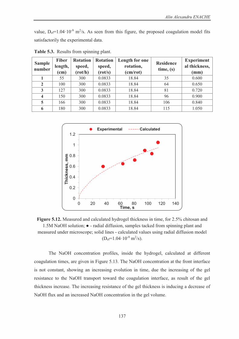
Alin Alexandru ENACHE
137
value, Def=1.04·10-9 m2/s. As seen from this figure, the proposed coagulation model fits
satisfactorily the experimental data.
Table 5.3. Results from spinning plant.
Sample number
Fiber length, (cm)
Rotation speed, (rot/h)
Rotation speed, (rot/s)
Length for one rotation, (cm/rot)
Residence time, (s)
Experimental thickness,
(mm) 1 55 300 0.0833 18.84 35 0.600 2 100 300 0.0833 18.84 64 0.650 3 127 300 0.0833 18.84 81 0.720 4 150 300 0.0833 18.84 96 0.900 5 166 300 0.0833 18.84 106 0.840 6 180 300 0.0833 18.84 115 1.050
Figure 5.12. Measured and calculated hydrogel thickness in time, for 2.5% chitosan and 1.5M NaOH solution; ● - radial diffusion, samples tacked from spinning plant and
measured under microscope; solid lines - calculated values using radial diffusion model (Def=1.04·10-9 m2/s).
The NaOH concentration profiles, inside the hydrogel, calculated at different
coagulation times, are given in Figure 5.13. The NaOH concentration at the front interface
is not constant, showing an increasing evolution in time, due the increasing of the gel
resistance to the NaOH transport toward the coagulation interface, as result of the gel
thickness increase. The increasing resistance of the gel thickness is inducing a decrease of
NaOH flux and an increased NaOH concentration in the gel volume.
0
0.2
0.4
0.6
0.8
1
1.2
0 20 40 60 80 100 120 140
Thic
knes
s, m
m
Time, s
Experimental Calculated

Mathematical Modelling of the Chitosan Fiber Formation by Wet-Spinning
138
The modelling and simulation study of the chitosan hydrogel wet-spinning described
in this paragraph, evidenced an acceptable agreement between the calculated and the
measured data on a laboratory wet-spinning unit. This is proving that the proposed model,
based on the Second Fick Law, associated to the hypothesis of instantaneous reaction
between the NaOH and chitosan –NH3+ moieties is adequate in the calculation of fiber
coagulation step of the wet-spinning process.
Figure 5.13 NaOH concentration profiles inside the hydrogel (2.5 wt. % chitosan and 1.5M NaOH).
0.00
0.30
0.60
0.90
1.20
1.50
0.00 0.20 0.40 0.60 0.80 1.00
CN
aOH
, (m
ol/L
)
r, (mm)
t = 35 s t = 64 s t = 81 st = 96 s t = 106 s t = 115 s

Alin Alexandru ENACHE
139
GENERAL CONCLUSIONS AND PERSPECTIVES

Mathematical Modelling of the Chitosan Fiber Formation by Wet-Spinning
140
The chitosan is a biomaterial that has been proved to be very useful in practical
applications, so that its processing, properties and utilizations are the subject of a large
number of published studies. Among the chitosan physical states used in practice, the
hydrogels present a particular importance. These are usually prepared by coagulation of
aqueous chitosan solutions. The experimental studies evidenced that, among the factors
influencing the hydrogel properties, an important one is the coagulation kinetics.
In spite of its importance, the number of publications investigating the coagulant
transport in chitosan hydrogels is relatively low. The present work brings some contributions
to the enrichment of data regarding the engineering process of chitosan hydrogels and
chitosan fibers manufacturing.
The principal conclusions of the experimental and theoretical investigations
described in the previous chapters are the following:
1) The rheological study of chitosan hydrogels evidenced that the hydrogel hardness
increases with the increase of the chitosan concentration and with the increase of the sodium
hydroxide concentration. This involves that two chitosan hydrogels, obtained in the same
conditions but containing different polymer mass fractions, will have different resistances
to mass transport by diffusion (in particular, different values of the coagulant diffusion
coefficient, during coagulation process).
2) The hydrogel structure images obtained by confocal laser scanning microscopy
and scanning electron microscopy highlighted the appearance of some microstructure with
non-homogeneities inside the hydrogels in the diffusion direction. These microstructures are
influencing the diffusion properties of the hydrogel. The gel zone in the vicinity of the
surface in contact with the sodium hydroxide (front interface) is denser and opposes a higher
resistance to diffusion, as compared with the gel zone in the neighborhood of (ending) gel
surface in contact with chitosan (dope) solution (coagulation interface). Therefore, the value
of the coagulant diffusion coefficient is variable across the gel thickness and is expected to
increase, during the coagulation process, from the front interface toward the coagulation
interface.
3) A first set of NaOH diffusion coefficient values were determined from
experiments consisting in the NaOH release from gel samples impregnated with different
concentrations of sodium hydroxide, immersed in a volume of distilled water under stirring.
The diffusion NaOH coefficient in the gel was calculated from the measured time evolution

Alin Alexandru ENACHE
141
of NaOH concentration released from the gel (by the intermediate of the measured pH of the
solution).
Nevertheless, the quality of the obtained results is rather modest, these presenting a
significant dispersion and a poor reproducibility. These is explained by several factors: the
experimental error in the measurement of the pH, the unsteady character of the process, the
limited mixing of the liquid, the non-homogeneities occurring in the gel structure appearing
during the coagulation process (see chapter 2), the possible changes in the gel structure
during the interval between their preparation and their use in experiments, the errors in the
measurement of disk thickness, the changes in the NaOH concentration in the solution due
to the absorption of carbon dioxide from air etc. These results were considered rather
uncertain, so more accurate methods were adopted, based on the kinetics of chitosan
coagulation process.
4) A second set of experiments used in the determination of coagulant diffusion
coefficient were performed by a more accurate method, using a parallelepiped shaped,
transparent diffusion cell and an optical microscope provided with on-line computer
interface. By coagulation experiments with the coagulant transport along the cell (linear
diffusion), several important kinetic specificities of the chitosan coagulation from acid
aqueous solutions were evidenced. The coagulation kinetics (displacement speed of the
coagulation front) was found to be faster at lower chitosan concentrations and higher
coagulation agent (base) concentrations.
5) The decrease of the coagulation front speed with the increase of chitosan
concentration is explained by the increased number of NH3+ moieties to be neutralized,
combined with a slightly higher resistance opposed by solid phase to coagulant diffusion
(lower value of NaOH diffusion coefficient in the gel). However, the dependence of
coagulation front speed on chitosan concentration is not linear. At a given coagulation agent
concentration and coagulation time, the ratio of the gel thicknesses obtained for two chitosan
concentrations is smaller than the reversed chitosan concentrations ratio.
6) The effect of NaOH concentration growth in the solution used as coagulation
agent, from 1M to 7M, keeping the chitosan concentration constant at 1 %, is a significant
increase of mass flux on the front interface and a less important increase of the flux on the
coagulation interface. The flux on the coagulation interface, when using NaOH solution 7M,
is only slightly superior to that corresponding to the solution 1M, thus explaining the value

Mathematical Modelling of the Chitosan Fiber Formation by Wet-Spinning
142
of gel thickness, not very different of that obtained with the coagulant concentration 1M.
The difference between the NaOH fluxes on the two hydrogel extremities appears due to the
amount of NaOH accumulated inside the gel, which is superior to the amount consumed in
the coagulation reaction, the ratio between the two quantities rising with the NaOH
concentration in the solution used for coagulation.
All these observations occur as consequence of the controlling effect of the coagulant
transport in the gel, toward the coagulation interface, on the overall process kinetics.
7) The experimental data evidenced that the increase of the gel thickness is faster on
the first interval of coagulation process, due to the smaller diffusion distance of coagulant
between the front interface and the coagulation interface. At longer coagulation times, the
transport distance inside the gel is larger, the resistance opposed to coagulant transport
increases and the growth rate of the hydrogel is decreasing, becoming almost constant at the
end of the coagulation process, where the curves have approximately linear shapes.
8) The modeling and simulation studies confirmed that the chitosan coagulation
process is adequately described by the second law of Fick, associated with the hypothesis of
instantaneous reaction between NaOH and NH3+ groups of the chitosan chains in the dope.
The proposed mathematical model of the coagulation process includes the resistances to the
NaOH transport, appearing both in the liquid phase (NaOH solution) at the gel vicinity and
inside the growing hydrogel stratus.
9) The parameter estimation studies, together with pH measurements performed in
immerged NaOH aqueous solutions inside the prepared hydrogels, indicated that the NaOH
partition coefficient, K, between NaOH solution and chitosan hydrogel is close to unity, so
in this modeling and simulation study the value K=1 was assumed. This is in agreement with
the theoretical interpretation of the partition coefficient for non-adsorbed solutes and was
supported by a weak sensitivity of the gel thickness evolution in respect with K, in the
vicinity of the value K=1, evidenced by process simulations.
10) The obtained NaOH diffusion coefficient values in the chitosan gel are in an
acceptable agreement with published data and the theoretical predictions by published
correlations. Constructing the graphs diffusion coefficient - chitosan concentration and
extrapolating to null chitosan concentration, there were obtained the values 1.9 10-9 m2∙s-1
for the solution 1M and 1.76∙10-9 m2∙s-1 for the 7M solution. These are in a reasonable
agreement with the value of the NaOH diffusion coefficient in the solution 1M reported in

Alin Alexandru ENACHE
143
literature (1.75∙10-9 m2·s-1) and the one estimated from published values of ions diffusivities
(2.125∙10-9 m2·s-1).
11) Among the published relations proposed for the estimation of the diffusion
coefficients in the gels, based on the obstruction theory, the most appropriate for the NaOH
diffusion in chitosan hydrogel, proved to be the one formulated by Mackie and Mears, which
is approaching our data with a difference between 8 and 9 %.
12) The study of the chitosan coagulation in cylindrical geometry (radial diffusion
of sodium hydroxide) evidenced that diffusion coefficient values determined from radial
coagulation experiments are lower than those obtained from linear coagulation, a result
reported also by other authors. We believe that this occurs due to combined influences of
transport geometry and structural non-homogeneity of chitosan gel, evidenced
experimentally. Thus, in the calculations of the cylindrical coagulation, it is recommended
to use diffusion coefficient values obtained from specific experiments performed with
systems having the same geometry.
13) The modelling and simulation study of the chitosan hydrogel wet-spinning
conducted to results in an acceptable concordance with the measured data on a laboratory
unit. This is proving that the proposed model can be used in the calculation of the coagulation
step of the fiber formation process by wet spinning.
The investigations developed in this work could be continued with further researches
regarding:
(1) The influence of the chitosan properties (acetylation degree, average molecular weight)
and temperature on the coagulation kinetics.
(2) More detailed modelling of coagulation process by taking into consideration the
structural heterogeneity of the gels.
(3) New research regarding the prediction of the diffusion coefficient in the chitosan
hydrogel by free volume theory and hydrodynamic theories respectively (by determination
using molecular analysis of the parameters involved in this theoretical models).
(4) Further studies of the wet spinning process. Experimental and theoretical investigations
aiming to obtain more accurate prediction of the coagulant mass transfer coefficients
between the liquid solution and the gel filament, during the wet-spinning process.

Mathematical Modelling of the Chitosan Fiber Formation by Wet-Spinning
144
REFERENCES Agboh O. C., Qin Y., (1997), Chitin and chitosan fibers, Polymers for Advanced Technologies, vol. 8, pp. 355-365. Agrawal P., Strijkers G. J., Nicolay K., (2010), Chitosan-based systems for molecular imaging, Adv. Drug Deliv. Rev., vol. 62, pp. 42–58. Aiba S., (1991), Studies on chitosan: 3. Evidence for the presence of random and block copolymer structures in partially N-acetylated chitosans, Int. J. Biol. Macromol, vol. 13, pp. 40-44. Aiba S., (1992), Studies on chitosan: 4. Lysozymic hydrolysis of partially N-acetylated chitosans, Int. J. Biol. Macromol, vol. 14, pp. 225-228. Aleman J. et al., (2007), Definitions of terms relating to the structure and processing of sols, gels, networks, and inorganic-organic hybrid materials, Pure Appl. Chem., vol. 79, pp. 1801–1829. Alfrey Jr. T., Gurnee E. F., Lloyd W. G., (1966), Diffusion in Glassy Polymers, Journal of Polymer Science Part C: Polymer Symposia, vol.12, pp. 249-261, Altenberger A. R., Tirrell M., (1984), On the Theory of Self‐Diffusion in A Polymer Gel, The Journal of Chemical Physics, vol. 80, pg. 2208. Amiji M.M., (1995), Pyrene fluorescence study of chitosan self-association in aqueous solution, Carbohyd Polym, vol. 26, pp. 211-213. Amsden B., (1998a), Solute Diffusion in Hydrogels: An Examination of The Retardation Effect, Polymer Gels and Networks, vol. 6, pp. 13-43. Amsden B., (1998b), Solute Diffusion within Hydrogels. Mechanisms and Models, Macromolecules, vol. 31, pp. 8382-8395. Amsden B., (2002), Modeling solute diffusion in aqueous polymer solutions, Polymer, vol. 43, pp. 1623-1630. Anitha A., Sowmya S., Kumar S.P.T., Deepthi S., Chennazhi K.P., Ehrlich H., Tsurkan M., Jayakumar R., (2014), Chitin and chitosan in selected biomedical applications, Progress in Polymer Science, vol. 39, Issue 9, pp. 1644-1667. Anthonsen M. W., Vårum K. M. Hermansson A. M., Smidsrød O., Brant D. A., (1994), Aggregates in acidic solutions of chitosans detected by static laser light scattering, Carbohydr. Polym., vol. 25 (1), pp. 13-23. Arbia W. et al., (2013), Chitin Recovery Using Biological Methods, Food Technol. Biotechnol., vol. 51 (1), pp. 12–25.

Alin Alexandru ENACHE
145
Arora A., Padua G. W., (2010) Review: Nanocomposites in Food Packaging, Journal of Food Science, vol. 75 (1), pp. 43-49. Atiyeh B. S., Costagliola M., Hayek S. N., Dibo S. A., (2007), Effect of silver on burn wound infection control and healing: Review of the literature, Burns, vol. 33 (2), pp. 139-148. Baldrick, P., (2010), The safety of chitosan as a pharmaceutical excipient. Regulatory Toxicology and Pharmacology, vol. 56, pp. 290-299. Berger J., Reist M., Mayer J. M., Felt O., Peppas N. A., Gurny R., (2004a), Structure and interactions in covalently and ionically crosslinked chitosan hydrogels for biomedical applications, Eur. J. Pharm. Biopharm., vol. 57 (1), pp. 19-34. Berger J., Reist M., Mayer J. M., Felt O., Gurny R., (2004b), Structure and interactions in chitosan hydrogels formed by complexation or aggregation for biomedical applications, Eur. J. Pharm. Biopharm., vol. 57 (1), pp. 35-52. Bernkop-Schnürch A., Dünnhaupt S., (2012), Chitosan-based drug delivery systems, Eur. J. Pharm. Biopharm., vol. 81, pp. 463–469. Berthold A., Cremer K., Kreuter J., (1996), Preparation and characterization of chitosan microspheres as drug carrier for prednisolone sodium phosphate as model for anti-inflammatory drugs, Journal of Controlled Release, vol. 39 (1), pp. 17-25. Bhattarai N., Edmondson D., Veiseh O., Matsen F. A., Zhang M. Q., (2005), Electrospun chitosan-based nanofibers and their cellular compatibility, Biomaterials, vol. 26, pp. 6176-6184. Bhattarai N., Gunn J., Zhang M., (2010), Chitosan-based hydrogels for controlled, localized drug delivery. Advanced Drug Delivery Reviews, vol. 62, pp. 83–99. Bird R. B., Stewart W. E., Lightfoot E. N., (2002), Transport Phenomena, John Wiley & Sons, p. 686 Bodmeier R., Chen H., Paeratakul O., (1989), A Novel Approach to the Oral Delivery of Micro- or Nanoparticles, Pharmaceutical Research, vol. 6 (5), pp. 413-417. Bumgardner J. D., Wiser R., Gerard P. D., Bergin P., Chestnutt B., Marini M., Ramsey V., Elder S.H., Gilbert J.A., (2003), Chitosan: potential use as a bioactive coating for orthopaedic and craniofacial/dental implants. Journal of Biomaterials Science, Polymer Edition 2003, vol. 14 (5), pp. 423-438. Cai J., Zhang L., (2005), Rapid Dissolution of Cellulose in LiOH/Urea and NaOH/Urea Aqueous Solutions, Macromol. Biosci., vol. 5, pp. 539–548. Cai J., Zhang L., (2006), Unique Gelation Behavior of Cellulose in NaOH/Urea Aqueous Solution, Biomacromolecules, vol. 7, pp. 183–189. Casettari L., Illum L., (2014), Chitosan in nasal delivery systems for therapeutic drugs, J. Control. Release, vol. 190, pp. 189–200.

Mathematical Modelling of the Chitosan Fiber Formation by Wet-Spinning
146
Chatelet C., Damour O., Domard A., (2001), Influence of the degree of acetylation on some biological properties of chitosan films, Biomaterials, vol. 22, pp. 261-268. Chenite A., Buschmann M., Wang D., Chaput C., Kandani N., (2001), Rheological characterisation of thermogelling chitosan/glycerol-poshphate solution, in Carbohydrate Polymers, vol. 46, pp. 39-47. Cho J., Heuzey M. C., Bégin A., Carreau P. J., (2006), Viscoelastic properties of chitosan solutions: Effect of concentration and ionic strength, J. Food Eng., vol. 74, pp. 500-515. Clague D. S. and Phillips R. J., (1996), Hindered diffusion of spherical macromolecules through dilute fibrous media, Phys. Fluids, vol. 8 (7), pp. 1720-1731. Cohen M. H., Turnbull D. J., (1959), Molecular Transport in Liquids and Glasses, Chem. Phys., vol. 31, pg. 1164. Cook G. J., (1968), Handbook of textiles fibres. 1. Naturel Fibres, Fourth edition - Merrow Publishing Co.LTD, England Crank J., (1975), The Mathematics of Diffusion, 2nd, New York, ed. Oxford: Clarendon Press. Crescenzi V., Imbriaco D., Velasquez C. L., Dentini M., Ciferri A., (1995), Novel types of polysaccharidic assemblies, Macromol. Chem. Phys., vol. 196, pp. 2873–2880. Crescenzi V., Paradossi G., Desideri P., Dentini, M., Cavalieri F., Amici E., Lisi R., (1997), New hydrogels based on carbohydrate and on carbohydrate-synthetic polymer networks, Polym. Gels Netw., vol. 5, pp. 225–239. Croisier F., Jerome C., (2013), Chitosan-based biomaterials for tissue engineering, Eur. Polym. J., vol. 49, pp. 780–792. Cukier R. I., (1984), Diffusion of Brownian spheres in semidilute polymer solutions, Macromolecules, vol. 17, pp. 252-255. Cussler E.L., (1997), Diffusion, Mass Transfer in Fluids Systems, 2nd ed., Cambridge, Cambridge University Press, p.162, 166 and 237. Dal Pozzo A., Vanini L., Fagnoni M., Guerrini M., De Benedittis A., Muzzarelli R., (2000), Preparation and characterization of poly(ethylene glycol)-crosslinked reacetylated chitosans, Carbohydr. Polym., vol. 42, pp. 201–206. Dash M., Chiellini F., Ottenbrite R. M., Chiellini E., (2011), Chitosan - A versatile semi-synthetic polymer in biomedical applications, Prog. Polym. Sci., vol. 36, pp. 981–1014. Denuziere A., Ferrier D., Domard, A., (1996) Chitosan-chondroitin sulfate and chitosanhyaluronate polyelectrolyte complexes. Physico-chemical aspects, Carbohydrate Polymers, vol. 29, pp. 317-323.

Alin Alexandru ENACHE
147
Desbrieres J., (2002), Viscosity of semiflexible chitosan solutions: Influence of concentration, temperature, and role of intermolecular interactions, Biomacromolecules, vol. 3, pp. 342-349. Domard A., Domard M., (2001a), Chitosan: Structure–Properties Relationship and Biomedical Applications. In Biomaterials, Dimitriu, S., New York, Ed. M. Dekker Press, pg. 187. Domard A., (1997), Chitosan interactions, In Domard, A.; Robert, G. A.; Varum, K. M., Advances in chitin science II, Lyon, Eds. Jacques André. Domard A., Domard M., (2002), Chitosane: Structure-Properties Relationship and Biomedical Applications, In Dumitriu, S. (ed.) Polymeric Biomaterials, New York, Marcel Dekker pp. 187-212. Domard A., Vachoud L., (2001b), In Uragami, T., Kurita, K., and Fukamizo, T., EDs., Chitin and Chitosan in Life Science, Tokyo, Kodansha Sci. Ltd, pp. 12-19. Dos Santos Z. M., Caroni A. L., Pereira M. R., Da Silva D. R., Fonseca J. L., (2009), Determination of deacetylation degree of chitosan: a comparison between conductometric titration and CHN elemental analysis, Carbohydrate Research., vol. 344 (18), pp. 2591–2595. Drogoz A., David, L., Rochas C., Domard A., Delair T., (2007), Polyelectrolyte Complexes from Polysaccharides: Formation and Stoichiometry Monitoring, Langmuir, vol. 23 (22), pp. 10950-10958. Duan J., Liang X., Cao Y., Wang S., Zhang L., (2015), High Strength Chitosan Hydrogels with Biocompatibility via New Avenue Based on Constructing Nanofibrous Architecture, Macromolecules, vol. 48, pp. 2706−2714. Dudhani A. R., Kosaraju S. L., (2010), Bioadhesive chitosan nanoparticles: Preparation and characterization, Carbohydrate Polymers., vol. 81 (2), pp. 243-251. Dumitriu S., Chornet E., (1996), Polyionic hydogels as supports for enzyme immobilization, In. Muzzarelli R. A. A (Ed.), Chitin Enzymology, vol. 2, Italy, Atec Edizioni, pp. 527–542. Dumitriu S., Chornet E., (2000), Polyonic hydrogels as support for enzyme immobilization, Chitin. Enzymol, vol. 2, pp. 527-542. Dumitriu S. (2001), In Severian Dumitriu (ed.), Polymeric Biomaterials, 2nd,New York, CRC Press. Elias H. G., (2008), Macromolecules: Volume 3: Physical Structures and Properties, Wiley-VCH, p 699. Enache A. A., David L., Puaux J.-P., Banu I., Bozga G., (2018a), “Kinetics of chitosan coagulation from aqueous solutions”, in Journal of Applied Polymer Science, vol. 135 (16), DOI:10.1002/app.46062.
Mathematical Modelling of the Chitosan Fiber Formation by Wet-Spinning
148
Enache A. A., David L., Puaux J.-P, Banu I., Bozga G., (2018b), „A modelling study of chitosan wet spinning process”, Bull UPB, ACCEPTED. Fary A.D., (1996), The Diffusional Properties of Sodium Hydroxide, Doctor’s Dissertation, The Institute of Paper Chemistry, Appleton, Wisconsin. Fick A., (1855), Ueber Diffusion, Annalen der Physik, vol. 170, pp. 59-86. Fricke H. A., (1924), Mathematical Treatment of the Electric Conductivity and Capacity of Disperse Systems I. The Electric Conductivity of a Suspension of Homogeneous Spheroids, Phys. Rev., vol. 24, pp. 575. Fujita H., (1961), Diffusion in polymer-diluent systems, Adv. Polym. Sci., Bd. 3, S. 1-47. Geankoplis C. J., (1993), Transport Processes and Unit Operations, 3rd Edition, New Jersey, Prentice-Hall Englewood Cliffs, pag 450. Geng X. Y., Kwon O. H., Jang J. H., (2005), Electrospinning of chitosan dissolved in concentrated acetic acid solution, Biomaterials, vol. 26, pp. 5427-5432. Griffiths P. C., Stilbs P., Chowdhry B. Z., Snowden M. J., (1995), PGSE-NMR Studies of Solvent Diffusion in Poly(N-Isopropylacrylamide) Colloidal Microgels, Colloid and Polymer Science, vol. 273, pp. 405-411. Grinsted R. A., Clark L., Koenig J. L., (1992), Study Of Cyclic Sorption-Desorption Into Poly(Methyl Methacrilate) Rods Using NMR Imaging Macromolecules, Macromolecules, vol. 25, pp. 1235-1241. Guenet J. M., (1992), Thermoreversible gelation of polymers and biopolymers. 2 ed., London, Academic Press, p 280. Hadwiger L. A., (2013), Plant science review: Multiple effects of chitosan on plant systems: Solid science or hype. Plant Sci., vol. 208, pp. 42–49. Hagège R., (2004), Fibres à usage techniques. Fibres, fils et tissus textiles. Techniques de l'Ingénieur, Plastiques et Composites A 3 980. Hayes E. R., Davies D. H., Munroe V. G., (1978), Organic acid solvent systems for chitosan., editors. In: Muzzarelli RAA, Pariser ER editors. Proceedings of the 1st International Conference on Chitin and Chitosan, Cambridge, Massachesetts, pp. 103-106. Helander I. M., Nurmiaho-Lassila E. L., Ahvenainen R., Rhoades J., Roller S., (2001), Chitosan disrupts the barrier properties of the outer membrane of Gram-negative bacteria, International Journal of Food Microbiology, vol. 71, pp. 235-244. Hermans J. J., (1947), Diffusion with Discontinuous Boundary, Journal of Colloid Science, vol. 2 (4), pp. 387–398. Heux L., Brugnerotto J., Desbrières J., Versal M. F., Rinaudo M., (2000), Solid state NMR for determination of degree of acetylation of chitin and chitosan, Biomacromolecules, vol. 1 (4), pp. 746–751.

Alin Alexandru ENACHE
149
Hirai A., Odani H., Nakajima A., (1991), Determination of degree of deacetylation of chitosan by 1H NMR spectroscopy, Polymer Bulletin, vol. 26 (1), pp. 87–94. Hirano S., Tsuchida H., Nagao N., (1989), N-Acetylation in Chitosan and the Rate of Its Enzymic-Hydrolysis, Biomaterials, vol. 10, pp. 574-576. Hirano S., Zhang M., Chung B. G., Kim S. K., (2000), The N-acylation of chitosan fibre and the N-deacetylation of chitin fibre and chitin–cellulose blended fibre at a solid state, Carbohydr. Polym., vol. 41 (2), pp. 175-179. Hon D. N. S., (1996), In: Dimitriu S. (ed.), Polysaccharides in medical applications., New York, Marcek Dekker Inc., p. 637. Hudson S. M., Jenkins D. W., (2002), Chitin and Chitosan. Encyclopedia of Polymer Science and Technology. 1, John Wiley & Sons Inc. Iliuta I., Larachi F., Grandjean B. P. A., (1999), Residence time, mass transfer and back-mixing of the liquid in trickle flow reactors containing porous particles, Chem. Eng. Sci., vol. 54, pp. 4099-4109. Illum L., Jabbal-Gill I., Hinchcliffe M., Fisher A.N., Davis S.S. (2001), Chitosan as a novel nasal delivery system for vaccines, Advanced Drug Delivery Reviews, vol. 51, pp. 81-96. Jayakumar R., Menon D., Manzoor K., Nair S. V., Tamura H., (2010), Biomedical applications of chitin and chitosan based nanomaterials - A short review, Carbohydr. Polym., vol. 82, pp. 227–232. Jarry C. et al., (2001), Effects of steam sterilization on thermogelling chitosan-based gels, Journal of Biomedical Materials Research, vol. 58, pp. 127-135. Jiang X., Chen L., Zhong W., (2003), A new linear potentiometric titration method for the determination of deacetylation degree of chitosan, Carbohydrate Polymers, vol. 54 (4), pp. 457–463. Jimtaisong A., Saewan N., (2014), Utilization of carboxymethyl chitosan in cosmetics, Int. J. Cosmet. Sci., vol. 36, pp. 12–21. Joanny J. F., (1989), The sol-gel transition, Physica B: Condensed Matter, vol. 156-157, pp. 381-385. Johansson L, Elvingson C, Lo¨froth J. E., (1991), Diffusion and interaction in gels and solutions. 3. Theoretical results on the obstruction effect, Macromolecules, vol. 24, pp. 6024-6029. Johnson E. M., Berk D. A., Jain, R. K., Deen W. M., (1996), Hindered diffusion in agarose gels: test of effective medium model, Biophys. J., vol. 70 (2), pp. 1017-1023.

Mathematical Modelling of the Chitosan Fiber Formation by Wet-Spinning
150
Jung W. J., Jo G. H, Kuk J. H., Kim Y. J., Oh K. T., Park R. D., (2007), Production of chitin from red crab shell waste by successive fermentation with Lactobacillus paracasei KCTC-3074 and Serratia marcescens FS-3, Carbohydr. Polym., vol. 68, pp 746–750. Kasaai M. R., (2008), A review of several reported procedures to determine the degree of N-acetylation for chitin and chitosan using infrared spectroscopy, Carbohydrate Polymers, vol. 71 (4), pp. 497–508. Kasaai M.R., (2007), Calculation of mark–houwink–sakurada (MHS) equation viscometric constants for chitosan in any solvent–temperature system using experimental reported viscometric constants data, Carbohydrate Polymers, vol. 68 (3), pp. 477–488. Kaur K., Dattajirao V., Shrivastava V., Bhardwaj U., (2012), Isolation and characterization of chitosan-producing bacteria from Beaches of Chennai, India. Enzyme Research, vol. 2012. Kean T., Thanou M., (2010), Biodegradation, biodistribution and toxicity of chitosan, Advanced Drug Delivery Reviews, vol. 62, pp. 3-11. Kim H. J., Lee H. C., Oh J. S., Shin B. A., Oh C. S., Park R. D., Yang K. S., Cho C. S., (1999), Polyelectrolyte complex composed of chitosan and sodium alginate for wound dressing application, J. Biomater. Sci. Polym., vol. 10, pp. 543-556. Kim S. S., Lee Y.M., Cho C. S., (1995), Synthesis and properties of semi-interpenetrating polymer networks composed of β-chitin and poly(ethylene glycol) macromer, Polymer, vol. 36, pp. 4497-4501. Kim D.B., Lee M.L., Lee W.S., Jo S.M., Kim B.C., (2002), Double crystallization behaviour in dry-jet wet spinning of cellulose/N-methylmorpholine-N-oxide hydrate solutions, European Polymer Journal, vol. 38 (1), pp. 109-119. Kiusalaas J., (2005), Numerical Methods in Engineering with Matlab, Cambridge, Cambridge University Press. Kishida A., Ikada Y., (2002), Hydrogels for biomedical and pharmaceutical applications, In Dumitriu, S., Ed, Polymeric biomaterials, 2nd, New York, CRC Press, pp 133-145. Khor E., (2001), Chitin: fulfilling a biomaterials promise, Amsterdam, Elsevier Science. Kjartansson G.T., Zivanovic S., Kristbergsson K., Weiss J., (2006), Sonication-assisted extraction of chitin from North Atlantic shrimps (Pandalus borealis), J. Agric. Food Chem., vol. 54, pp. 5894–5902. Klaveness J. N., Brudeli B. N., Smidsrod O. N., Varum K., Morten N.O., Mustaparta, E. N., (2004), Pharmaceutical compositions comprising an active agent and chitosan for sustained drug release of mucoadhesion, US20060293216 A1. Klokkevold P. R., Fukayama H., Sung E. C., Bertolami C. N., (1999), The effect of chitosan (poly-N-acetyl glucosamine) on lingual haemostasis in heparinized rabbits, J. Oral Maxillofac. Surg., vol. 57, pp. 49-52.

Alin Alexandru ENACHE
151
Knaul J. Z., Creber K A. M., (1997), Coagulation Rate Studies of Spinnable Chitosan Solutions, Journal of Applied Polymer Science, vol. pp. 66, 117–127. Knaul J. Z., (1998), Improved mechanical properties of chitosan fibers with applications to degradable radar countermeasure chaff, PhD Thesis, Royal Military College of Canada, Kingston, Ontario, Canada. Kofuji K., Akamine H., Qian C. J., Watanabe K., Togan Y., Nishimura M., Sugiyama I., Murata Y., Kawashima S., (2004), Therapeutic efficacy of sustained drug release from chitosan gel on local inflammation, International Journal of Pharmaceutics, vol. 272, pp. 65-78. Krieger T., (2014), Flow and Functional Models for Rheological Properties of Fluid Foods, In: Rao A., Rheology of fluid, Semisolid, and Solid Foods, Principles and Applications, 3 nd, Springer US. Kwon P. H., Lee S. H., Lee S. M., Park S. J., (1999), High strength fibers from chitosan derivatives, Kichin, Kitosan Kenkyu vol. 5, pp. 178-179. Kurahashi I., Seo H., (1985), Production of chitosan fiber, Fuji Spinning Co.Ltd. (Japanese Patent 60059123). Lahiji A., Sohrabi A., Hungerford D. S., Frondoza, C. G., (2000), Chitosan supports the expression of extracellular matrix proteins in human osteoblasts and chondrocytes, Journal of Biomedical Materials Research, vol. 51, pp. 586-595. Lauffer M. A., (1961), Theory of Diffusion in Gels, Biophys J., vol. 1, pp. 205-213. Langdon A. G, Thomas H. C., (1971), Self-Diffusion Studies of Gel Hydration and The Obstruction Effect, The Journal of Physical Chemistry, vol. 76, pp. 1821-1826. Lavertu M., Xia Z., Serreqi A. N., Berrada M., Rodrigues A., Wang D., Buschmann M. D., et al., (2003), A validated 1H NMR method for the determination of the degree of deacetylation of chitosan, Journal of Pharmaceutical and Biomedical Analysis, vol. 32 (6), pp. 1149–1158. Lee K. Y., Ha W. S., Park W. H., (1995), Blood Compatibility and Biodegradability of Partially N-Acylated Chitosan Derivatives, Biomaterials, vol. 16, pp. 1211-1216. Lee K. Y., Park W. H., Ha W. S., (1997), Polyelectrolyte complexes of sodium alginate with chitosan or its derivatives for microcapsules, J. Appl. Polym. Sci., vol. 63 (4), pp. 425-432. Lee S. H., (2000), The mechanism and characteristics of dry-jet wet spinning of chitosan fibers, Journal of the Korean Fiber Society, vol. 37, pp. 374-381. Li C., Han Q., Guan Y., Zhang Y., (2014), Thermal gelation of chitosan in an aqueous alkali-urea solution, Soft Matter, vol. 10, pp. 8245–8253.

Mathematical Modelling of the Chitosan Fiber Formation by Wet-Spinning
152
Li D., Xia Y. N., (2004), Electrospinning of nanofibers: Reinventing the wheel?, Advanced Materials, vol. 16, pp. 1151-1170. Liu C. K., Cuculo J. A., Smith B., (1989), Coagulation Studies for Cellulose in the Ammonia / Ammonium Thiocyanate (NH3 / NH4SCN) Direct Solvent System, J. Polym. Sci. Polym. Phys. Part B., vol. 27 (12), pp. 2493-2511. Lustig S. R., Peppas N. A., (1988), Solute diffusion in swollen membranes. IX. Scaling laws for solute diffusion in gels, J. Appl. Polym. Sci., vol. 36 (4), pp. 735-747. Mackie J. S., Meares P., (1955), The Diffusion of Electrolytes in A Cation-Exchange Resin Membrane, The Royal Society London A, vol. 232, pp. 498-509. Massaro L., Zhu X.X., (1999), Physical models of diffusion for polymer solutions, gels and solids, Prog. Polym. Sci., vol. 24, pp. 731–775. Mi F. L. et al., (2000), Fabrication and characterization of a sponge-like assymetric chitosan membrane as a wound dressing, Biomaterials, vol. 22, pp. 165-173.
Mi F. L., Shyu S. S., Wong T. B., Jang S. F., Lee S. T., Lu K. T., (1999), Chitosan–polyelectrolyte complexation for the preparation of gel beads and controlled release of anticancer drug. II. Effect of pH-dependent ionic crosslinking or interpolymer complex using tripolyphosphate or polyphosphate as reagent, J. Appl. Polym. Sci., vol. 74 (5), pp. 1093-1107. Ming B. C., (1960), Chitinfasern und chitosandruck, Faserforsh Textiltech, vol. 11, pp. 320-326. Mohammad F., (2013), Green Chemistry Approaches to Develop Antimicrobial Textiles Based on Sustainable Biopolymers-A Review, Ind. Eng. Res., vol. 52, pp. 5245–5260. Montembault A., Viton, C., Domard, A., (2005), Rheometric Study of the Gelation of Chitosan in Aqueous Solution without Cross-Linking Agent, Biomacromolecules, vol. 6 (2), pp. 653-662. Montembault A. et al., (2006), A material decoy of biological media based on chitosan physical hydrogels: application to cartilage tissue engineering, Biochimie, vol. 88, pp. 551-564. Muhr A. H., Blanshard J.M.V., (1982), Diffusion in gels, Polymer, vol. 23, pp. 1012-1026. Muñoz G., Valencia C., Valderruten N., Ruiz-Durántez E., Zuluaga F. (2015), Extraction of chitosan from Aspergillus niger mycelium and synthesis of hydrogels for controlled release of betahistine, Reactive and Functional Polymers, vol. 91–92, pp. 1–10. Muzzarelli R. A. A, Jeuniaux C., Gooday G. W., (1986), Chitin in nature and technology. New York, Plenum, p. 385. Muzzarelli R. A. A., (1998), Chitin and the human body. Advances in chitin science vol. 1,

Alin Alexandru ENACHE
153
Muzzarelli R. A. A., Muzzarelli C., (2005), Chitosan chemistry: Relevance to the biomedical sciences, In: Heinze T. (eds), Polysaccharides I. Advances in Polymer Science, vol 186. Springer, Berlin, Heidelberg. Muzzarelli R. A. A., (2009), Chitins and chitosans for the repair of wounded skin, nerve, cartilage and bone, Carbohydr. Polym., vol. 76, pp. 167–182. Nie J. et al., (2015), Orientation in multi-layer chitosan: morphology, mechanism and design principle, Sci. Rep., vol. 5, pp. 1-7. Nie J., Wang Z., Hu Q., (2016), Difference between Chitosan Hydrogels via Alkaline and Acidic Solvent Systems, Scientific Reports. Nwe N., Stevens W.F., Tokura S., Tamura H., (2008), Characterization of chitosan and chitosan– glucan complex extracted from the cell wall of fungus Gongronella butleri USDB 0201 by enzymatic method. Enzyme and Microbial Technology, vol. 42 (3), pp. 242–251. Nyström B, Moseley ME, Brown W, Roots J., (1981), Molecular Motion of Small Molecules in Cellulose Gels Studied By NMR, Journal of Applied Polymer Science, vol. 26, pp. 3385-3393. Ogston A. G., (1958), The spaces in a uniform random suspension of fibres, Trans. Faraday Soc., vol. 54, pp. 1754-1757. Ootani T., Yoneyama H., Kamo J., (1980), Production of formed product of chitosan. Mitsubishi Rayon Co. Japanese Patent 6106901. Ootani T., Yoneyama H. & Kamo J., (1981), Preparation of chitosan molded product. Mitsubishi Rayon Co. (Japanese Patent 56112937). Ottoy M. H., Vårum K. M., Smidsrød O., (1996a), Compositional heterogeneity of heterogeneously deacetylated chitosans, Carbohydrate Polymers, vol. 29 (1), pp. 17-24. Ottoy M. H., Varum K. M., Christensen B. E., Anthonsen M. W., Smidsrod, O., (1996b), Preparative and analytical size-exclusion chromatography of chitosans, Carbohydrate Polymers, vol. 31, pp. 253-261. Park S.K., (2001), Dry-jet wet spinning of aromatic polyamic acid fiber using chemical imidization, Polymer, vol. 42 (26), pp. 10087–10093. Patel A. K., (2015), Chitosan: Emergence as potent candidate for green adhesive market, Biochem. Eng. J., vol. 102, pp. 74–81. Patel A., Mequanint K., (2011), Hydrogel Biomaterials, Biomedical Engineering - Frontiers and Challenges, Prof. Reza Fazel (Ed.), InTech, DOI: 10.5772/24856. Available from: https://www.intechopen.com/books/biomedical-engineering-frontiers-and-challenges/hydrogel-biomaterials; accessed December 2017. Patrulea V., Ostafe V., Borchard G., Jordan O., (2015), Chitosan as a starting material for wound healing applications, Eur. J. Pharm. Biopharm., vol. 97, pp. 417–426.

Mathematical Modelling of the Chitosan Fiber Formation by Wet-Spinning
154
Paul D.R., (1968), Diffusion during the coagulation step of wet-spinning, J. Appl. Polym. Sci., vol. 12, pp. 383-402. Peppas N. A., (1986), Preface. In Peppas, N. A., Hydrogels in Medicine and Pharmacy: Vol. 1. Fundamentals, Boca Raton, FL, Ed. CRC Press. Phillips R. J., Deen W. M., Brady J. F., (1989), Hindered transport of spherical macromolecules in fibrous membranes and gels, AIChE J., vol. 35 (11), pp. 1761-1769. Picout D. R., Ross-Murphy S. B., (2003), Rheology of Biopolymer Solutions and Gels, Sci. World J., vol. 3, pp. 105-121. Pillai C. K. S., Paul W., Sharma C. P., (2009), Chitin and chitosan polymers: Chemistry, solubility and fiber formation, Progress in Polymer Science, vol. 34 (7), pp 641-678. Pillai C.K.S., Sharma C. P. (2009), Electrospinning of Chitin and Chitosan Nanofibres, Trends in Biomater. Artif. Organs, vol. 20, pp. 179-201. Prameela K., Mohan C. M., Smitha P. V., Hemalatha K. P. J., (2010), Bioremediation of shrimp biowaste by using natural probiotic for chitin and carotenoid production an alternative method to hazardous chemical method, IJABPT, vol. 1, ppp. 903–910. Prego C., Torres D., Fernandez-Megia E., Novoa-Carballal R., Qui E., Alonso M.J., (2006), Chitosan-PEG nanocapsules as new carriers for oral peptide delivery: Effect of chitosan pegylation degree, Journal of Controlled Release, vol. 111 (3), pp. 299-308. Qin W., Shen Y., Fei L., (1993), NMR Imaging of acetone diffusion process in polycarbonate, Chinese Journal of Polymer Science, vol.11, pp. 358-363. Rabbe D. et al., (2005), The crustacean exoskeleton as an example of a structurally and mechanically graded biological nanocomposite material, Acta Materialia, vol. 53, pp. 4281-4292. Raafat D., Sahl H. G. (2009), Chitosan and its antimicrobial potential? a critical literature survey, Microbial Biotechnology, vol. 2 (2), pp. 186-201. Radhakumary C., Nair P. D., Reghunadhan Nair C. P., Mathew S., (2012), Chitosan-graft-poly(vinyl acetate) for hemodialysis applications, Journal of Applied Polymer Science, vol. 125 (3), pp. 2022-2033. Ravi Kumar M. N. V. (2000), A review of chitin and chitosan applications. Reactive and Functional Polymers, vol. 46 (1), pp. 1–27. Regiel A., Kyzioł A., (2013), Chitosan-silver nanocomposites – modern antibacterial materials, CHEMIK, vol. 67 (8), pp. 683–692. Rabea E. I., Badawy M. E. T., Stevens C. V., Smagghe G., Steurbaut W., (2003), Chitosan as antimicrobial agent: Applications and mode of action, Biomacromolecules, vol. 4, pp. 1457-1465.

Alin Alexandru ENACHE
155
Rao M.S., Muñoz J., Stevens W.F., (2000), Critical factors in chitin production by fermentation of shrimp biowaste, Appl. Microbiol. Biotechnol., vol. 54, pp. 808–813. Rao S. B, Sharma C. P., (1997), Use of chitosan as a biomaterial: studies on its safety and hemostatic potential, J. Biomed. Mater. Res., vol. 34, pp. 21-28. Rigby G. W., (1936), Process for the preparation of films and filaments and products thereof, US Patent 2 040 880. Rinaudo M., (2006), Chitin and chitosan: properties and applications, Prog. Polym. Sci., vol. 31, pp. 603–632. Rivas Araiza R. N., Alcouffe P., Rochas C., Montembault A., David L., (2010), Micron Range Morphology of Physical Chitosan Hydrogels, Langmuir, vol. 26, pp. 17495–17504 Roberts G. A. F., (1992), Chitin Chemistry, 1st ed, London, MacMillan. Roberts G. A. F. (1997), In: Domard, A., Roberts, G.A.F., Vårum, K.M., Chitosan production routes and their role in determining the structure and properties of the product, 7th ICCC, Lyon, France, pp 22-31. Rotte J. W., Tummers G. L. J., Dekker J. L., (1969), Mass transfer to a moving continuous cylinder, Chemical Engineering Science, vol. 24, pp. 1009-1015. Ross-Murphy S. B., (1991), Physical gelation of synthetic and biological macromolecules, In: D.DeRossi, K. K., Y. Osada and A. Yamauchi, Polymer Gels; Fundamentals and Biomedical Applications, New York, Plenum Press, pp 21-40. Rusu-Balaita L., Desbrières J., Rinaudo M., (2003), Formation of a biocompatible polyelectrolyte complex: chitosan-hyaluronan complex stability, Polymer bulletin, vol. 50 (1-2), pp. 91-98. Sajomsang W., Ruktanonchai U. R., Gonil P., Nuchuchua O., (2009), Mucoadhesive property and biocompatibility of methylated N-aryl chitosan derivatives, Carbohydrate Polymers, vol. 78 (4), pp. 945–952. Sannan T., Kurita K., Iwakura Y., (1975), Studies on chitin, 1. Solubility change by alkaline treatment and film casting, Die Makromolekulare Chemie, vol. 176 (4), pp. 1191-1195. Sannan T., Kurita K., Iwakura Y., (1976), Studies on chitin, 2. Effect of deacetylation on solubility, Macromolecular Chemistry and Physics, vol. 177 (12), pp 3589-3600. Saranya N., Moorthi A., Saravanan S., Devi M. P., Selvamurugan N., (2010), Chitosan and its derivatives for gene delivery, International Journal of Biological Macromolecule, vol. 48 (2), pp. 234-238. Sarhan A. A. et al. (2009), Phase transfer catalyzed heterogeneous N-deacetylation of chitin in alkaline solution, Reactive & Functional Polymers, vol. 69, pp. 358-363.

Mathematical Modelling of the Chitosan Fiber Formation by Wet-Spinning
156
Schatz C., Pichot C., Delair T., Viton C., Domard A., (2003), Static Light Scattering Studies on Chitosan Solutions: From Macromolecular Chains to Colloidal Dispersions, Langmuir, vol. 19, pp. 9896-9903. Schatz C., Lucas J. M., Viton C., Domard A., Picho, C., Delair T., (2004), Formation and Properties of Positively Charged Colloids Based on Polyelectrolyte Complexes of Biopolymers, Langmuir, vol. 20, pp. 7766-7778. Sereni N., Enache A., Sudre G., Montembault A., Rochas C., Durand P., Perrard M.H., Bozga G., Puaux J.-P., Delair T., David L., (2017). Dynamic structuration of physical chitosan hydrogels, Langmuir, vol. 33 (44), pp 12697–12707. Serrero A., Bayon Y., David L., Domard A., Gravagna P., Montanari S., Trombotto S., (2009), Polysaccharides-based adhesives for biological applications, In: Adhesion Society. Meeting, Proceedings, 32nd Annual Meeting of the Adhesion Society, Inc: February 15 - 18, 2009, Savannah, GA, Shin Y., Yoo D. I., Min K., (1999), Antimicrobial finishing of polypropylene nonwoven fabric by treatment with chitosan oligomer, Journal of Applied Polymer Science, vol. 74, pp. 2911- 2916. Sorlier P., Denuzière A., Viton C., Domard A., (2001), Relation between the degree of acetylation and the electrostatic properties of chitin and chitosan, Biomacromolecules, vol. 2, pp 765–772. Strand S. P., Vandvik M. S., Varum K. M., Ostgaard K., (2001), Screening of chitosans and conditions for bacterial flocculation, Biomacromolecules, vol. 2, pp. 126-133. Suginta W., Khunkaewla P., Schulte A., (2012), Electrochemical Biosensor Applications of Polysaccharides Chitin and Chitosan, Chem. Rev., vol. 113, pp. 5458–5479. Suh J. K. F., Matthew H. W. T., (2000), Application of chitosan-based polysaccharide biomaterials in cartilage tissue engineering: a review, Biomaterials, vol. 21, pp. 2589-2598.
Shu X. Z., Zhu K. J., (2000), A novel approach to prepare tripolyphosphate/chitosan complex beads for controlled release drug delivery, International Journal of Pharmaceutics, vol. 201 (1), pp. 51-58. Shu X. Z., Zhu K. J., (2002), Controlled drug release properties of ionically cross-linked chitosan beads: the influence of anion structure, International Journal of Pharmaceutics, vol. 233 (1-2), pp. 217-225. Synowiecki J., Al-Khateeb N. A. A. Q., (2000), The recovery of protein hydrolysate during enzymatic isolation of chitin from shrimp Crangon crangon processing discards – Commercial uses and potential application, Food Chem., vol. 68, pp. 147–152. Ta H. T., Dass C. R., Dunstan D. E., (2008), Injectable chitosan hydrogels for localised cancer therapy, Journal of Controlled Release, vol. 126 (3), pp. 205-216.

Alin Alexandru ENACHE
157
Teng D., (2011), From chitin to chitosan, In: K. Yao, J. Li, F. Yao, Y. Yin (Eds.), Chitosan- based hydrogels: Functions and application, Boca Raton, Florida: CRC Press, pp. 233. Terada D., Kobayashi H., Zhang K., Tiwari A., Yoshikawa C., Hanagata N., (2012), Transient charge-masking effect of applied voltage on electrospinning of pure chitosan nanofibers from aqueous solutions, Science and Technology of Advanced Materials, vol. 13, number 1. Terbojevich M., Carraro C., Cosani A., (1989), Solution studies of chitosan 6-O-sulfate, Makromol. Chem., vol. 190, pp. 2847-2855 Tokura S., Seo H., (1984), Manufacture of chitosan fiber and film. Fuji Spinning Co.Ltd. (Japanese Patent 59116418). Tokura S. et al., (1987), Preparation and some properties of variously deacetylated chitin fibers. Sen'i Gakkaishi, vol. 43, pp. 288-293. Tsai D. S., Strieder W., (1985), Effective conductivities of random fiber beds, Chem. Eng. Commun., vol. 40, pp. 207-218. Tsuchida E., Abe K. (1986) Polyelectrolyte complexes. In: Wilson, A D and Prosser, H J (Eds.) Development in ionic polymers-2, Elsevier Applied Science Publishers, London and New York, Chapter 5; pp. 191–263. Urreaga J. M., De la Orden M. U., (2006), Chemical interactions and yellowing in chitosan-treated cellulose, European Polymer Journal, vol. 42 (10), pp. 2606–2616. Van Den Broek L. A. M., Knoop, R. J. I., Kappen, F. H. J., Boeriu, C. G., (2015), Chitosan films and blends for packaging material, Carbohydr. Polym., vol. 116, pp. 237–242. Vârum K. M., Myhr M. M., Hjerde R. J. N., Smidsrod O., (1997), In vitro degradation rates of partially N-acetylated chitosans in human serum, Carbohydrate Research, vol. 299, pp. 99-101. Vârum K. M., Smidsrød O., (2004) Structure-Property Realtionship in Chitosan, In: Dumitriu S., Polysaccharides: Structural Diversity and Functional Versality, Sherbrooke, Ed. Marcel Dekker, 2004. Venault A., Bouyer D., Pochat-Bohatier C., Vachoud L., Faur C., (2012), Investigation of chitosan gelation mechanisms by a modeling approach coupled to local experimental measurement, AIChE J., vol. 58, pp. 2226-2240 Vermonden T., Censi R., Hennink W. E., (2012), Hydrogels for protein delivery, Chem. Rev., vol. 112, pp. 2853-2888. Vongchan P., Sajomsang W., Subyen D., Kongtawelert P., (2002), Anticoagulant activity of a sulfated chitosan, Carbohydrate Research., vol. 337 (13), pp. 1239-1242. Vrentas J. S., Duda J. L. J., (1977), Diffusion in polymer—solvent systems. I. Reexamination of the free-volume theory, Polym. Sci., vol. 15, pp. 403-416.
Mathematical Modelling of the Chitosan Fiber Formation by Wet-Spinning
158
Wan Ngah W. S., Teong L. C., Hanafiah M. A. K. M., (2011), Adsorption of dyes and heavy metal ions by chitosan composites: A review, Carbohydr. Polym., vol. 83, pp. 1446–1456. Wedmore I., McManus J.G., Pusateri A.E., Holcomb J.B., (2006), A special report on the chitosan-based hemostatic dressing: experience in current combat operations, J. Trauma, vol. 60 (3), pp. 655-658. Westrin B. A., Axelsson A., Zacchi G., (1994), Diffusion measurement in gels, J. Control Release, vol. 30, pp. 189-199. Yamaguchi R. Hirano S., Arai Y., Ito T., (1978), Chitosan Salt Gels Thermally Reversible Gelation of Chitosan, Agricultural and Biological Chemistry, vol.42 (10), pp. 1981-1982. Yao K. D., Tu H., Cheng F., Zhang J. W., Liu, J., (1997), pH-sensitivity of the swelling of a chitosan-pectin polyelectrolyte complex, Die Angewandte Makromolekulare Chemie, vol. 245 (1), pp. 63-72. Yasuda H., Lamaze C. E., Ikenberry L. D., (1968), Permeability of solutes through hydrated polymer membranes. Part I. Diffusion of sodium chloride, Die Makro Chem., vol. 118, pp. 19-35. Yuan Y., Chesnutt B. M., Haggard W. O., Bumgardner J. D., (2011). Deacetylation of chitosan: material characterization and in vitro evaluation via albumin adsorption and pre-osteoblastic cell cultures, Materials, vol. 4, pp. 1399-1416. Sajomsang W., Ruktanonchai U. R., Gonil P., Nuchuchua O., (2009), Mucoadhesive property and biocompatibility of methylated N-aryl chitosan derivatives, Carbohydrate Polymers, vol.78 (4), pp. 945–952. Zhang H., Li Y., Zhang X., Liu B., Zhao H., et al., (2016) Directly determining the molecular weight of chitosanwith atomic force microscopy, Front Nanosci Nanotech, vol. 2 (3), pp. 123-127.

Alin Alexandru ENACHE
159
LIST OF PUBLISHED WORKS
- Enache A. A., David L., Puaux J.-P., Banu I., Bozga G., “Kinetics of chitosan coagulation from aqueous solutions”, in Journal of Applied Polymer Science, vol. 135, no. 16, 2018, DOI:10.1002/app.46062, Impact Factor: 1.86.
- Sereni N., Enache A. A., Sudre G., Montembault A., Rochas C., Durand P., Perrard M.H., Bozga G., Puaux J.-P., Delair T., David L., (2017). „Dynamic structuration of physical chitosan hydrogels”, Langmuir, vol. 33 (44), pp 12697–12707, Impact Factor: 3.833.
- Enache A. A., David L., Puaux J.-P., Banu I., Bozga G., (2018), „A modelling study of chitosan wet spinning process”, U.P.B. Sci. Bull., Series B, Vol. 80, Iss. 2, pp. 13-26.
- Enache A.A., David L., Puaux J.-P, Banu I., Bozga G., “A Kinetic Study of Chitosan Coagulation from Aqueous Solutions”, Conferinta RICCCE 20, Poiana Brasov, Sept. 2017.


![Cytocompatibility of Chitosan and Collagen-Chitosan ...forms the highly porous structure of the scaffolds[13] Two percent (w/v) of chitosan was prepared by dissolving chitosan in 0.2](https://img.dokumen.tips/doc/110x75/5e3f1725786dcc56c068fc16/cytocompatibility-of-chitosan-and-collagen-chitosan-forms-the-highly-porous.jpg)