Mathematical Modeling of Controlled Longitudinal Motion of a Paraglider

Computational Mathematics and Modeling, Vol. 24, No. 3, July, 2013

MATHEMATICAL MODELING OF CONTROLLED LONGITUDINAL MOTIONOF A PARAGLIDER

A. M. Formal’skii and P. V. Zaitsev

A paraglider consists of a harness and a wing. Both bodies are assumed perfectly rigid. They are con-nected by suspension lines, which are regarded as perfectly rigid weightless rods. These rods are rigidlyattached to the harness and to the wing. The paraglider model is thus a single rigid body with threedegrees of freedom. A propeller motor is rigidly attached to the harness. The thrust developed by the pro-peller is applied to the harness. The thrust vector maintains constant orientation relative to the harness.We develop a mathematical model of a paraglider moving in the longitudinal plane. Stationary motionregimes are identified assuming constant thrust. A thrust control is proposed that stabilizes the paragliderflight at a given altitude. Regions of asymptotic stability of paraglider motion at a constant altitude areconstructed in the plane of feedback coefficients (allowing for delay). Regions ensuring a given stabilitymargin are also constructed in this plane. Simulation results are presented for paraglider flight.

Introduction

The development of remote-controlled and pilotless aircraft is a topical direction in modern aviation [1, 2].The paraglider is one of such promising aircraft. In this article we investigate the paraglider dynamics and designa paraglider control by considering a mathematical model of planar longitudinal motion of the aircraft.

The single-link paraglider model investigated in this article consists of a wing and a harness. Both bodies areassumed perfectly rigid; they are connected by suspension lines, which are modeled by perfectly rigid rods rigidlyconnected to both the harness and the wing. Our mechanical model of a paraglider is thus a single rigid body,which has three degrees of freedom in planar longitudinal motion.

A motor rigidly fixed to the harness develops thrust by means of a propeller. The thrust vector developed bythis propeller maintains a constant orientation relative to the harness.

The wing, and thus the entire apparatus, is subjected to a lift force and aerodynamic drag. These forces, as wellas the thrust and the harness drag, create moments relative to the center of mass, which balance one another understationary flight conditions. Given a certain thrust under stationary conditions, the paraglider moves horizontally,i.e., at a constant altitude. This constant-thrust horizontal flight, however, is not asymptotically stable in relation toaltitude. It may be stabilized by controlling the magnitude of the thrust vector.

Initially, during takeoff, the paraglider harness moves on the ground (rolling on wheels). Having attaineda certain sufficiently high velocity, the apparatus lifts off, because the lift force now exceeds the weight. Thesystem is thus subject to a one-sided constraint in the takeoff section, which is incorporated in the mathematicalmodel.

We develop a computer simulation program for the longitudinal motion of a paraglider, including options forflight animation.

Research Institute of Mechanics, Lomonosov Moscow State University, Moscow, Russia

Translated from Nelineinaya Dinamika i Upravlenie, No. 7, pp. 383–396, 2010.

418 1046-283X/13/2403–0418 c© 2013 Springer Science+Business Media New York

MATHEMATICAL MODELING OF CONTROLLED LONGITUDINAL MOTION OF A PARAGLIDER 419

1. Mathematical Model of Paraglider

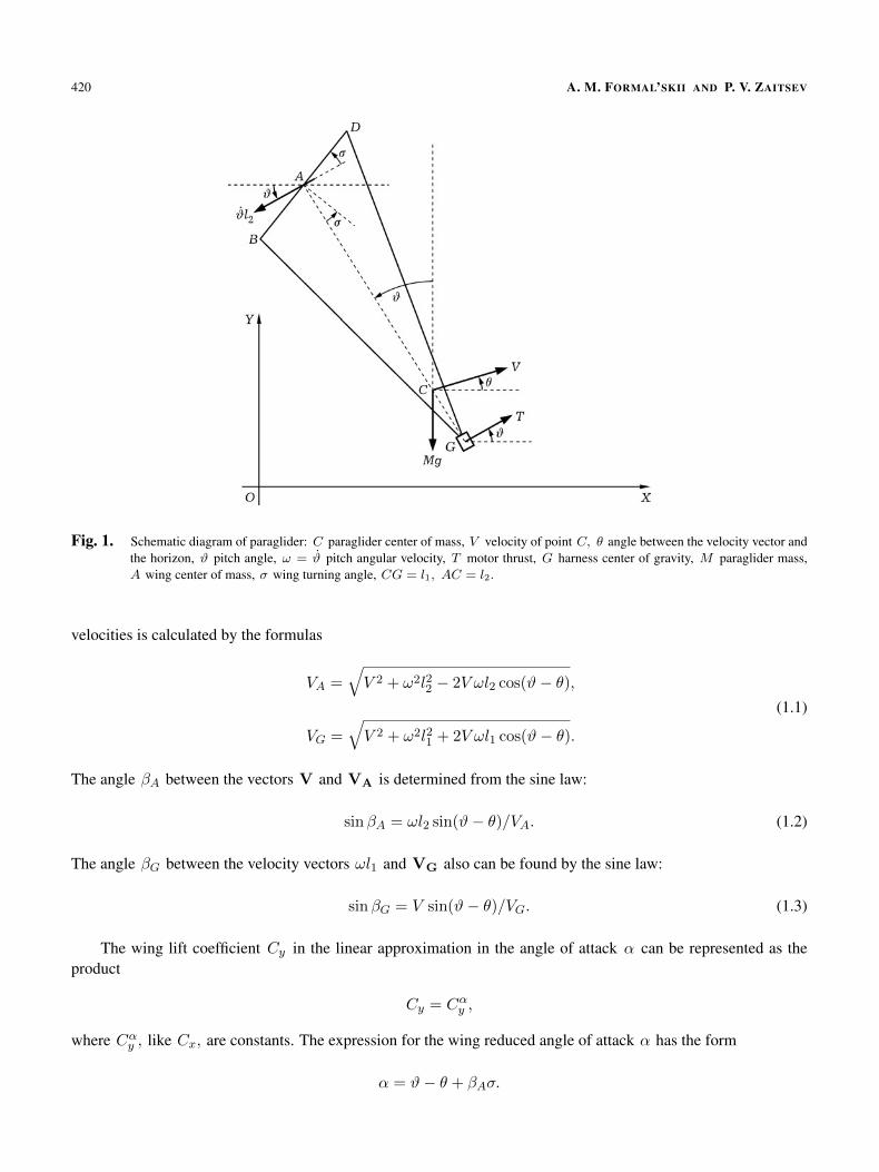
Figure 1 is a schematic diagram of a paraglider. The wing in this diagram is shown as the straight-line segmentBD centered at the point A (lateral view). Assume that the point A is the center of mass of the wing. We assumethat the wing lift

P = Cy1

2ρV 2

AS,

and the wing drag

Q = Cx1

2ρV 2

AS

are both applied at the center A of the plate. The quantities Cy and Cx are the lift and drag coefficients [3, 4];

the quantity1

2ρV 2

AS is the dynamic pressure, with ρ the air density, VA the velocity of the point A relative to theoncoming stream, S the wing area.

The point where the lift P and the drag Q are applied naturally changes with the velocity and the orientationof the wing. We ignore this factor in our model, because the moment of these forces relative to the paraglider centerof mass “weakly” depends on the application point if the distance CA between the center of mass and the wing islarge relative to the wing size BD.

Denote by G the center of mass of the harness. The distance GA is denoted by L. Let m1 be the mass of theharness, m2 the mass of the wing, and m1 +m2 = M. Then the distance l1 from the paraglider center of mass Cto the point G is

l1 =m2L

m1 +m2=m2L

M.

Denote by l2 the distance CA, equal to L = l1. If the wing mass m2 is substantially less than the harness massm1, then the distance l1 is substantially less than the distance l2 : l1 << l2. The center of mass of the entireparaglider C is thus close to the harness G. By T we denote the thrust developed by the motor. We assume thatthe thrust T is applied at the harness center of mass G and its vector always remains perpendicular to the straightline GA.

Denote by J he paraglider moment of inertia relative to its center of mass C, by g the free fall acceleration.If the suspensions lines are of different lengths, then the angle between the wing and the straight line AG is not aright angle; we denote by σ the angle between the perpendicular to the wing and the straight line AG (see Fig. 1).The turning of the wing in the longitudinal plane through some angle σ may be exploited to adjust the lift. In ourmodel the angle σ is assumed constant.

We introduce a coordinate system XOY fixed relative to the earth; the OX axis points horizontally in thedirection of paraglider motion and the OY axis points vertically up. Let x and y be the coordinates of theparaglider center of mass C, V the velocity of the center of mass, θ the angle between the center of mass velocityvector and the positive direction of the OX axis. The pitch angle, i.e., the angle between the vertical axis OYand the straight line CA measured counterclockwise, is denoted by ϑ (see Fig. 1). The pitch angular velocity ϑ isdenoted by ω.

If the paraglider turns around its center of mass in flight, the absolute velocity VA of the center of the wing Aand also the absolute velocity VG of the harness center of mass G are not equal to the velocity V of the paraglidercenter of mass C.

The velocity vectors VA and VG of the points A and G are the sum of the velocity vector of the paraglidercenter of mass and the velocity vectors of the points A and G relative to the center of mass. The magnitude of these

420 A. M. FORMAL’SKII AND P. V. ZAITSEV

Fig. 1. Schematic diagram of paraglider: C paraglider center of mass, V velocity of point C, θ angle between the velocity vector andthe horizon, ϑ pitch angle, ω = ϑ pitch angular velocity, T motor thrust, G harness center of gravity, M paraglider mass,A wing center of mass, σ wing turning angle, CG = l1, AC = l2.

velocities is calculated by the formulas

VA =√V 2 + ω2l22 − 2V ωl2 cos(ϑ− θ),

VG =√V 2 + ω2l21 + 2V ωl1 cos(ϑ− θ).

(1.1)

The angle βA between the vectors V and VA is determined from the sine law:

sinβA = ωl2 sin(ϑ− θ)/VA. (1.2)

The angle βG between the velocity vectors ωl1 and VG also can be found by the sine law:

sinβG = V sin(ϑ− θ)/VG. (1.3)

The wing lift coefficient Cy in the linear approximation in the angle of attack α can be represented as theproduct

Cy = Cαy ,

where Cαy , like Cx, are constants. The expression for the wing reduced angle of attack α has the form

α = ϑ− θ + βAσ.


The term βA in this sum arises due to the changes in the direction of the incident stream velocity as the wing rotatesabout the paraglider center of mass C. The sine of this angle (see (1.2)) is proportional to the pitch angular velocityω and the distance l2 from the point A to the center of mass C if the velocity VA is close to the velocity V.

At each point of the wing there is naturally its own “local” angle of attack, but it does not differ much fromthe angle ϑ − θ + βA + σ if the wing span BD is small compared with the distance l2. The distance l2 in turnincreases as the suspension lines become longer and the paraglider center of mass comes closer to the harness.In this article we assume that at all points of the wing the angle of attack is given by

α = ϑ− θ + βAσ.

To allow for the nonlinear dependence of the lift and drag coefficients on the angle of attack, we need to knowthe polar that relates the coefficients Cy and Cx for different angles of attack [3, 4].

In the equations of motion that follow we allow for the harness drag

QG = CxG1

2ρV 2

GS,

where CxG = const is the harness drag coefficient. The harness lift is assumed zero.Let us derive the differential equations describing planar longitudinal motion of the paraglider. To this end we

apply the general theorems of the dynamics of a system of point masses the theorem on the motion of the center ofmass and the theorem of the variation of the moment of momentum of the system relative to the center of mass [5].

The equation of motion of the paraglider center of mass C projected on the tangent to its trajectory has theform

MV = −Mg sin θ + T cos(ϑ− θ) + Cαy (ϑ− θ + βA + σ)1

2ρV 2

AS sinβA

− Cx1

2ρV 2

AS cosβA − CxG1

2ρS cos(ϑ− θ − βG) +Ry sin θ −Rx cos θ. (1.4)

The first term in the right-hand side of Eq. (1.4) describes the projection of the paraglider force of gravity Mg

onto the tangent to the trajectory; the second term describes the projection of the thrust T on the tangent; the thirdterm describes the projection of the lift; the fourth and fifth terms describe the projections on the tangent of thedrag applied to the wing and the harness respectively. Ry is the vertical component of the reaction of the supportsurface, which is nonzero on the takeoff section of paraglider motion, i.e., when it accelerates for takeoff and theharness is rolling on wheels on the ground. Rx is the horizontal component of the force applied by the groundto the harness — it describes the resistance to the rolling motion of the harness on the ground. The force Ry isassumed positive if it points vertically up. In numerical simulation we assume that the paraglider lifts off the groundas soon as this quantity changes its sign and becomes negative. Once the paraglider has lifted off the ground,

Ry = Rx = 0.

The equation of motion of the paraglider center of mass C projected on the normal to the trajectory has the form

MV θ = −Mg cos θ + T sin(ϑ− θ) + Cαy (ϑ− θ + βA + σ)1

2ρV 2

AS cosβA

+ Cx1

2ρV 2

AS sinβA − CxG1

2ρS sin(ϑ− θ − βG) +Ry cos θ +Ry cos θ +Rx sin θ. (1.5)


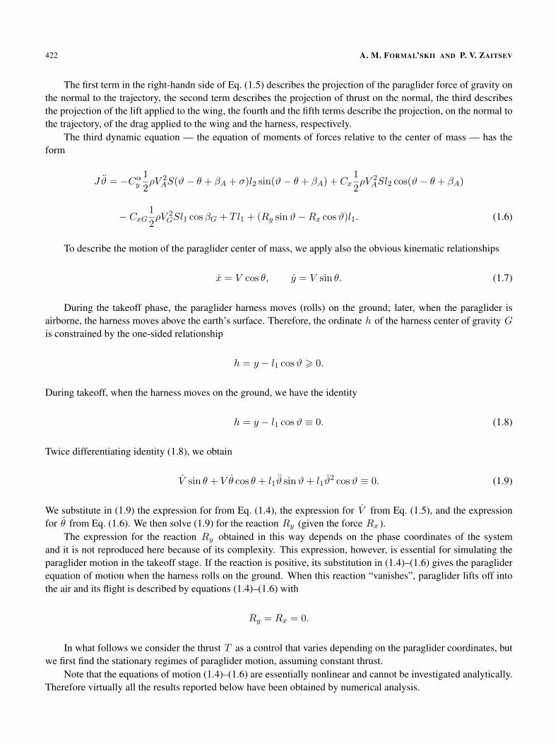
The first term in the right-handn side of Eq. (1.5) describes the projection of the paraglider force of gravity onthe normal to the trajectory, the second term describes the projection of thrust on the normal, the third describesthe projection of the lift applied to the wing, the fourth and the fifth terms describe the projection, on the normal tothe trajectory, of the drag applied to the wing and the harness, respectively.

The third dynamic equation — the equation of moments of forces relative to the center of mass — has theform

Jϑ = −Cαy1

2ρV 2

AS(ϑ− θ + βA + σ)l2 sin(ϑ− θ + βA) + Cx1

2ρV 2

ASl2 cos(ϑ− θ + βA)

− CxG1

2ρV 2

GSl1 cosβG + T l1 + (Ry sinϑ−Rx cosϑ)l1. (1.6)

To describe the motion of the paraglider center of mass, we apply also the obvious kinematic relationships

x = V cos θ, y = V sin θ. (1.7)

During the takeoff phase, the paraglider harness moves (rolls) on the ground; later, when the paraglider isairborne, the harness moves above the earth’s surface. Therefore, the ordinate h of the harness center of gravity Gis constrained by the one-sided relationship

h = y − l1 cosϑ > 0.

During takeoff, when the harness moves on the ground, we have the identity

h = y − l1 cosϑ ≡ 0. (1.8)

Twice differentiating identity (1.8), we obtain

V sin θ + V θ cos θ + l1ϑ sinϑ+ l1ϑ2 cosϑ ≡ 0. (1.9)

We substitute in (1.9) the expression for from Eq. (1.4), the expression for V from Eq. (1.5), and the expressionfor θ from Eq. (1.6). We then solve (1.9) for the reaction Ry (given the force Rx ).

The expression for the reaction Ry obtained in this way depends on the phase coordinates of the systemand it is not reproduced here because of its complexity. This expression, however, is essential for simulating theparaglider motion in the takeoff stage. If the reaction is positive, its substitution in (1.4)–(1.6) gives the paragliderequation of motion when the harness rolls on the ground. When this reaction “vanishes”, paraglider lifts off intothe air and its flight is described by equations (1.4)–(1.6) with

Ry = Rx = 0.

In what follows we consider the thrust T as a control that varies depending on the paraglider coordinates, butwe first find the stationary regimes of paraglider motion, assuming constant thrust.

Note that the equations of motion (1.4)–(1.6) are essentially nonlinear and cannot be investigated analytically.Therefore virtually all the results reported below have been obtained by numerical analysis.


2. Stationary Uncontrolled Flight (with Constant Thrust)

Let us find the stationary motion of the paraglider with constant motor thrust T = const .

Applying the dynamic equations (1.4)–(1.6), we seek the stationary flight regime in the form

V ≡ const,

ϑ ≡ const,

θ ≡ const.

(2.1)

The stationary regime (2.1), if it exists, represents uniform translational motion of the paraglider along a straightline that makes an angle θ with the horizontal axis OX. Under conditions (2.1) we have

V = 0,

ϑ = ω = 0,

θ = 0.

(2.2)

From expressions (1.1)–(1.3) it follows that, with ω = 0

VA = V,

VG = V,

βA = 0,

βG = ϑ− θ.

(2.3)

Substituting (2.2), (2.3) in Eq. (1.4), we obtain the following relationships linking the thrust T, the angles ϑ, θ,and the velocity V in the stationary regime (recall that in flight Ry = Rx = 0):

−Mg sin θ + T cos(ϑ− θ)− (Cx + CxG)1

2ρV 2S = 0. (2.4)

From equality (2.4) we obtain

1

2ρV 2S =

T cos(ϑ− θ)−Mg sin θ

Cx + CxG

or (2.5)

1

2ρT =

(Cx + CxG)ρV 2S + 2Mg sin θ

2 cos(ϑ− θ).

Substituting (2.2), (2.3) in Eq. (1.5), we obtain

−Mg cos θ + T sin(ϑ− θ) + Cαy (ϑ− θ + σ)1

2ρV 2S = 0. (2.6)


Under conditions (2.2), (2.3) Eq. (1.6) takes the form

1

2ρV 2S

[Cxl2 cos(ϑ− θ)− CxGl1 cos(ϑ− θ)− Cyα(ϑ− θ + σ)l2 sin(ϑ− θ)

]= 0. (2.7)

Equations (2.5)–(2.7) are relatively easy to solve if we seek the stationary flight regime at constant altitude,i.e., when θ ≡ 0. Given θ ≡ 0 and using relationships (2.5), we obtain from Eq. (2.7) an equation for the pitchangle ϑ : (

1− CxGl1Cxl2

)cos2 ϑ+

(1 +

CxGCx

)l1l2−CαyCx

(ϑ+ σ) sinϑ cosϑ = 0. (2.8)

From relationships (2.8) it follows that the stationary value of the pitch angle ϑ depends on three ratiosCxG/Cx, C

αy /Cx, l1/l2 and the wing orientation angle σ, while being independent of the thrust T or the veloc-

ity V.Equation (2.8) cannot be solved analytically for the unknown pitch angle ϑ. However, the root of this equa-

tion can be found numerically, by constructing the dependence of the left-hand side of Eq. (2.8) on ϑ for givenparaglider parameters.

Setting θ = 0 in (2.5), (2.6), we can apply these relationships with the known value of ϑ to compute the thrustT when the paraglider flies horizontally, i.e., at a constant altitude:

T =Mg

CαyCx

(1 +

CxGCx

)−1

(ϑ+ σ) cosϑ+ sinϑ

. (2.9)

Given the pitch angle ϑ, expression (2.5) determines the relationship between thrust and velocity. Having com-puted the thrust from (2.9), we can then apply the first relationship in (2.5) to calculate the corresponding veloc-ity V.

Relationships (2.5)–(2.7) also produce stationary flight regimes with velocity vector angle θ 6= 0. To this end,it is better to solve Eqs. (2.5)–(2.7) “backward”. Specifying some angle θ, we substitute it in Eqs. (2.5)–(2.7).Then these three equations contain three unknowns: the pitch angle ϑ, the velocity V, and the thrust T, which

we assume unknown for the given angle θ. Then the dynamic pressure1

2ρV 2S from the first relationship (2.5) is

substituted in the two equations (2.6)–(2.7).Only two unknowns remain in these two equations: the pitch angle ϑ and the thrust T. The thrust T enters

these equations linearly and is therefore easily eliminated. The one nonlinear equation obtained after eliminatingthe thrust contains a single unknown — the pitch angle ϑ. This nonlinear equation can be solved numerically.Having determined the angle ϑ, we can find the thrust T previously eliminated from both equations and thenapply the first formula (2.5) to find the velocity V.

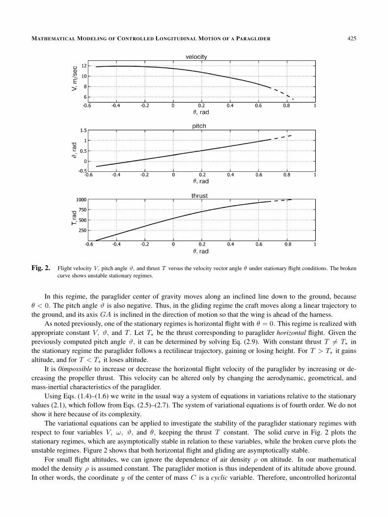
Figure 2 plots for stationary regimes the dependence of the flight velocity V, the pitch angle ϑ, and the thrustT on the velocity vector angle θ. The graphs have been constructed for σ = 0 and some hypothetical paragliderparameters (m1 = 100 kg, m2 = 7 kg, L = 7.3 m, S = 30 m2, Cαy = 1.2, Cx = 0.1, CxG = 0.1).

We see from Fig. 2 that as the thrust T increases the stationary angle θ becomes larger, but the paraglidervelocity V decreases. This decrease of paraglider velocity may be explained as follows: the increase of the angleθ increases the projection of the paraglider force of gravity on the tangent to the trajectory Mg sin θ, which isdirected opposite to the velocity (see Eq. (1.4) and the first relationship in (2.5)). For T = 0 there exists a stationarygliding regime with constant values of velocity V, pitch angle ϑ, and velocity vector angle θ (see Fig. 2).


Fig. 2. Flight velocity V, pitch angle ϑ, and thrust T versus the velocity vector angle θ under stationary flight conditions. The brokencurve shows unstable stationary regimes.

In this regime, the paraglider center of gravity moves along an inclined line down to the ground, becauseθ < 0. The pitch angle ϑ is also negative. Thus, in the gliding regime the craft moves along a linear trajectory tothe ground, and its axis GA is inclined in the direction of motion so that the wing is ahead of the harness.

As noted previously, one of the stationary regimes is horizontal flight with θ = 0. This regime is realized withappropriate constant V, ϑ, and T. Let T∗ be the thrust corresponding to paraglider horizontal flight. Given thepreviously computed pitch angle ϑ, it can be determined by solving Eq. (2.9). With constant thrust T 6= T∗ inthe stationary regime the paraglider follows a rectilinear trajectory, gaining or losing height. For T > T∗ it gainsaltitude, and for T < T∗ it loses altitude.

It is 0impossible to increase or decrease the horizontal flight velocity of the paraglider by increasing or de-creasing the propeller thrust. This velocity can be altered only by changing the aerodynamic, geometrical, andmass-inertial characteristics of the paraglider.

Using Eqs. (1.4)–(1.6) we write in the usual way a system of equations in variations relative to the stationaryvalues (2.1), which follow from Eqs. (2.5)–(2.7). The system of variational equations is of fourth order. We do notshow it here because of its complexity.

The variational equations can be applied to investigate the stability of the paraglider stationary regimes withrespect to four variables V, ω, ϑ, and θ, keeping the thrust T constant. The solid curve in Fig. 2 plots thestationary regimes, which are asymptotically stable in relation to these variables, while the broken curve plots theunstable regimes. Figure 2 shows that both horizontal flight and gliding are asymptotically stable.

For small flight altitudes, we can ignore the dependence of air density ρ on altitude. In our mathematicalmodel the density ρ is assumed constant. The paraglider motion is thus independent of its altitude above ground.In other words, the coordinate y of the center of mass C is a cyclic variable. Therefore, uncontrolled horizontal


motion (with T = T∗ = const) is indifferent to the coordinate y and is thus not asymptotically stable in relationto flight altitude.

3. Controlling Flight AltitudeStability of paraglider flight at the desired altitude can be ensured by controlling the motor thrust. Thrust

control stabilizing the paraglider flight at a given altitude is constructed as feedback in the deviations of the altitudeh of the harness G from the desired (specified) altitude and the velocity vector angle θ :

T = Ts − kh(h− hd)− kθθ. (3.1)

Here Tx is the given constant thrust, equal to T∗ or close to this value,

h = y − l1 cosϑ, (3.2)

hd is the desired flight altitude of the harness G above the ground, kh, kθ are the constant feedback coefficients.The coefficient kh should be positive (this follows from physical considerations). Indeed, if the flight altitudeexceeds the desired altitude, the thrust should be reduced; if the altitude is less than desired, the thrust should beincreased. The numerical analysis described below constructs the asymptotic stability regions and confirms thisconclusion. It follows from the second relationship in (1.7) that for small angles θ the derivative of the altitude yof the paraglider center of mass C above ground (the ascent velocity) is

y ≈ V θ,

i.e., it is proportional to the velocity vector angle θ. Thus, the last term in the control law (3.1) for small values ofthe angle θ is proportional to the vertical component y of the velocity of the center of mass C.

Under the control (3.1) the system (1.4)–(1.7), (3.2) has the stationary flight regime

V ≡ const, θ ≡ const,

ϑ ≡ const, ω ≡ 0,

y ≡ const, h ≡ const,

T ≡ const .

(3.3)

The values ϑ, T, and V are successively determined from relationships (2.8), (2.9), and (2.5). In horizontal flightthe stationary thrust is T.

It follows from equality (3.1) that the harness stationary altitude h is determined by the relationship

h = hd +1

kh(Ts − T∗). (3.4)

From (3.4) we obtain that the error

∆h = |h− hd|

in tracking the specified altitude hd decreases as the difference |Ts − T∗| approaches zero and (or) as the alti-tude feedback coefficient kh increases. We know from control theory [6], however, that if the position feedbackcoefficient kh (kh > 0) is chosen too large, the stationary regime (3.3) may become unstable.


Fig. 3. Asymptotic stability region and regions with stability margin 0, 1, 0, 2, or 0, 3 constructed in the plane of the feedback coeffi-cients kh, kθ.

Examination of the stability regions constructed below also confirms this assertion. The error

∆h = |h− hd| = 0,

if and only if Ts = T∗. If Ts > T∗, then it follows from expression (3.4) that the paraglider flight altitude in thestationary regime is greater than the specified hd ; conversely, if Ts < T∗ the altitude h is less than the specified hd.

Note that since the paraglider characteristics are known only approximately, the thrust T∗ when the craft flieshorizontally can be determined only approximately. Therefore Ts in the control law (3.1) cannot be specifiedexactly equal to the altitude of paraglider’s horizontal flight.

Using Eqs. (1.4)–(1.6), the second kinematic equation (1.7), and relationships (3.1), (3.2) we can write theequations in variations with respect to the stationary regime (3.3). The system of variational equations is of fifthorder. It includes variational equations used to analyze the stability of the stationary horitonal flight without feed-back (3.1) — when

T = T∗ = const.

This system is too complex to be given here in full.The variational equations can be applied to investigate the stability of the paraglider stationary regime with

respect to the five variables V, ω, ϑ, θ, and h. Figure 3 shows the region of asymptotic stability in relation tothese variables; it has been constructed numerically from the variational equations in the plane of the feedbackcoefficients kh, kθ. We see from the figure, in particular, that the positive coefficient kh is bounded from abovefor each value of the coefficient kθ.

Figure 3 also shows the boundaries of the regions with given stability margins 0, 1, 0, 2, and 0, 3. These arethe regions where the system eigenvalues λi (i = 1, . . . , 5) are distant from the imaginary axis by at least 0, 1,

0, 2, or 0, 3 to the left. As the desired value of the stability margin increases, the corresponding region naturallyshrinks.

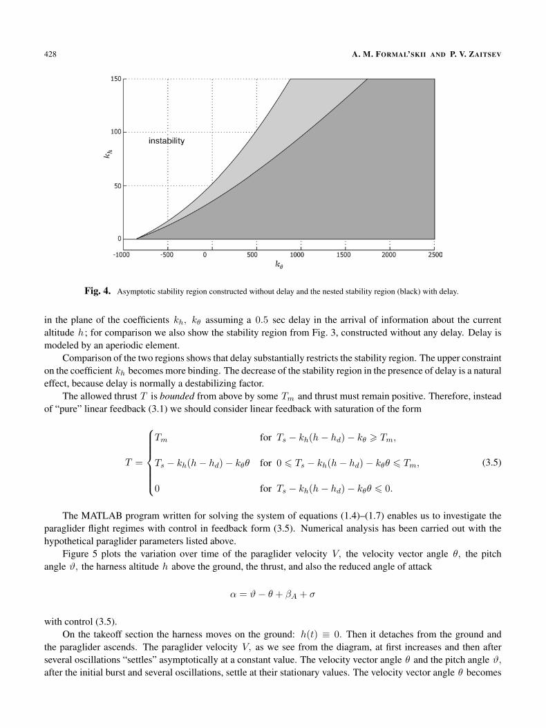
The control law (3.1) ignores the possible delay in the arrival of information about the current altitude h and(or) the velocity vector angle θ in the feedback loop. Figure 4 shows the asymptotic stability region constructed


Fig. 4. Asymptotic stability region constructed without delay and the nested stability region (black) with delay.

in the plane of the coefficients kh, kθ assuming a 0.5 sec delay in the arrival of information about the currentaltitude h ; for comparison we also show the stability region from Fig. 3, constructed without any delay. Delay ismodeled by an aperiodic element.

Comparison of the two regions shows that delay substantially restricts the stability region. The upper constrainton the coefficient kh becomes more binding. The decrease of the stability region in the presence of delay is a naturaleffect, because delay is normally a destabilizing factor.

The allowed thrust T is bounded from above by some Tm and thrust must remain positive. Therefore, insteadof “pure” linear feedback (3.1) we should consider linear feedback with saturation of the form

T =

Tm for Ts − kh(h− hd)− kθ > Tm,

Ts − kh(h− hd)− kθθ for 0 6 Ts − kh(h− hd)− kθθ 6 Tm,

0 for Ts − kh(h− hd)− kθθ 6 0.

(3.5)

The MATLAB program written for solving the system of equations (1.4)–(1.7) enables us to investigate theparaglider flight regimes with control in feedback form (3.5). Numerical analysis has been carried out with thehypothetical paraglider parameters listed above.

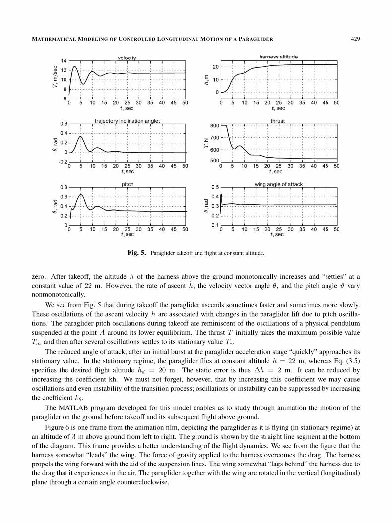
Figure 5 plots the variation over time of the paraglider velocity V, the velocity vector angle θ, the pitchangle ϑ, the harness altitude h above the ground, the thrust, and also the reduced angle of attack

α = ϑ− θ + βA + σ

with control (3.5).On the takeoff section the harness moves on the ground: h(t) ≡ 0. Then it detaches from the ground and

the paraglider ascends. The paraglider velocity V, as we see from the diagram, at first increases and then afterseveral oscillations “settles” asymptotically at a constant value. The velocity vector angle θ and the pitch angle ϑ,after the initial burst and several oscillations, settle at their stationary values. The velocity vector angle θ becomes


Fig. 5. Paraglider takeoff and flight at constant altitude.

zero. After takeoff, the altitude h of the harness above the ground monotonically increases and “settles” at aconstant value of 22 m. However, the rate of ascent h, the velocity vector angle θ, and the pitch angle ϑ varynonmonotonically.

We see from Fig. 5 that during takeoff the paraglider ascends sometimes faster and sometimes more slowly.These oscillations of the ascent velocity h are associated with changes in the paraglider lift due to pitch oscilla-tions. The paraglider pitch oscillations during takeoff are reminiscent of the oscillations of a physical pendulumsuspended at the point A around its lower equilibrium. The thrust T initially takes the maximum possible valueTm and then after several oscillations settles to its stationary value T∗.

The reduced angle of attack, after an initial burst at the paraglider acceleration stage “quickly” approaches itsstationary value. In the stationary regime, the paraglider flies at constant altitude h = 22 m, whereas Eq. (3.5)specifies the desired flight altitude hd = 20 m. The static error is thus ∆h = 2 m. It can be reduced byincreasing the coefficient kh. We must not forget, however, that by increasing this coefficient we may causeoscillations and even instability of the transition process; oscillations or instability can be suppressed by increasingthe coefficient kθ.

The MATLAB program developed for this model enables us to study through animation the motion of theparaglider on the ground before takeoff and its subsequent flight above ground.

Figure 6 is one frame from the animation film, depicting the paraglider as it is flying (in stationary regime) atan altitude of 3 m above ground from left to right. The ground is shown by the straight line segment at the bottomof the diagram. This frame provides a better understanding of the flight dynamics. We see from the figure that theharness somewhat “leads” the wing. The force of gravity applied to the harness overcomes the drag. The harnesspropels the wing forward with the aid of the suspension lines. The wing somewhat “lags behind” the harness due tothe drag that it experiences in the air. The paraglider together with the wing are rotated in the vertical (longitudinal)plane through a certain angle counterclockwise.


Fig. 6. A frame from the animation film.

This rotation produces the wing angle of attack and thus a lift that drives the wing upward. The suspensionlines apply this force to the harness, keeping it aloft.

Our mathematical model does not apply to the description of the paraglider motion on the ground, as it beginsmoving from rest. Simulation also shows that with small initial paraglider velocity V (0) the reduced angle ofattack

α = ϑ− θ + βA + σ

initially takes “large” values, so that linearization of the lift coefficient Cy by the angle of attack (Cy = Cαy α) isinappropriate.

The mathematical model is well-posed starting with the instant when the paraglider has already acceleratedto a sufficient velocity and its further motion on the ground is free from large oscillations in the pitch angle. Theparaglider flight at the specified altitude can be stabilized not only by the control (3.5), but also by feedback usingthe altitude h and its derivative h :

T =

Tm for Ts − kh(h− hd)− khh > Tm,

Ts − kh(h− hd)− khh for 0 6 Ts − kh(h− hd)− khh 6 Tm,

0 for Ts − kh(h− hd)− khh 6 0.

(3.6)

Expression (3.6) describes feedback using paraglider position and its derivative, which corresponds to a so-called PD (proportional-differential) controller. To realize the control law (3.6) we have to observe both the alti-tude of the harness above the ground (with an altimeter) and the rate of change of this altitude. It follows fromexpressions (1.7), (3.2) that for small angles θ, ϑ and small angular velocity ω the derivative h of the altitudeis proportional to the angle θ. The control laws (3.5) and (3.6) are thus close to each other. With accuracy toquantities of second order we may assume that the coefficients kh and kθ are related by a multiplier:

V : kh∼= V kθ.

Note that specifying hd as a function of time hd = hd(t) or range hd = hd(x) we can plan the takeofftrajectory, the marching regime, and the descent trajectory.


The altitude of an aircraft or a rocket is usually controlled by aerodynamic or fluid-dynamic elevators. Thealtitude of a paraglider, as we have shown above, can be effectively controlled by controlling the motor thrust.

This control option arises because the motor thrust is applied to the harness, while the lift is applied to thewing located above the harness. By changing the motor thrust we can alter the pitch angle and hence the lift actingon the wing, which in the end changes the paraglider flight altitude.

4. Conclusion

We have developed a mathematical model of the longitudinal motion of a paraglider. The stationary flightregimes have been obtained for constant thrust developed by the motor attached to the harness and their stabilityhas been investigated.

The thrust control has been constructed in feedback form, stabilizing the paraglider flight at the specifiedaltitude. Regions of asymptotic stability of the paraglider flying at constant altitude have been constructed in theplane of feedback coefficients. Results of paraglider flight simulations are reported.

The study has been supported by the Russian Foundation of Basic Research (grants 07-01-92167-NTsNI-a,09-01-00593-a, 10-07-00619-a).

REFERENCES

1. V. M. Lokhin, S. V. Man’ko, M. P. Romanov, I. B. Garnev, D. V. Evstigneev, and K. S. Kolyadin, “Promising systems and aggregatesbased on aircraft,” Perspektivnye Sistemy i Zadachi Upravleniya. Tematicheskii Vypusk, Izv. TRTU, No. 3, Izd. TRTU, Taganrog (2006).

2. G. V. Abramenko, D. V. Vasil’kov, and O. V. Voron’ko, Design of Complex Science-Based Technical Systems [in Russian], RFFI,Moscow (2006).

3. A. A. Lebedev and L. S. Chernobrovkin, Flight Dynamics of Pilotless Aircraft [in Russian], Mashinostroenie, Moscow (1973).4. S. M. Gorlin, Experimental Aeromechanics [in Russian], Vysshaya Shkola, Moscow (1970).5. N. V. Butenin, Ya. L. Luntz, and D. R. Merkin, A Course in Theoretical Mechanics. Dynamics [in Russian], Vol. 2, Nauka, Moscow

(1979).6. Ya. N. Roitenberg, Automatic Control [in Russian], Nauka, Moscow (1992).

Documents

Mathematical Modeling of Controlled Longitudinal Motion of a Paraglider