Cybernetics and Systems Analysis, Vol. 55, No. 6, November, 2019

MATHEMATICAL METHODS TO FIND OPTIMAL

CONTROL OF OSCILLATIONS OF A HINGED BEAM

(DETERMINISTIC CASE)�

G. Zrazhevsky,1

A. Golodnikov,2

and S. Uryasev3

UDC 519.9

Abstract. We consider several problem statements for the optimal controlled excitation of oscillations

of a hinged beam. Oscillations occur under the influence of several external periodic forces. In the

simplest statement, it is assumed that the structure of the beam is homogeneous. In a more complex

formulation, inhomogeneities (defects) on the beam are allowed. The goal of controlling

the oscillations of the beam is to provide a predetermined shape and a predetermined pointwise phase

of oscillations in a given frequency range. The problem is to determine the number of forces and their

characteristics (application, amplitude, and phase of oscillations), which provide the desired

waveform with a given accuracy. With the help of analytical mathematical methods, the problems

in question are reduced to simpler multiextremum problems of minimizing basic functionals, which can

be numerically solved using the multifunctional package AORDA PSG.

Keywords: vibrations, waveform, optimal actuation.

INTRODUCTION

Let us consider a problem about optimal controlled excitation of oscillations of a hinged beam. The problem is

a development of the approach proposed in [1]. By optimal control we understand providing a beam oscillation mode

such that the waveform is the most close to the desired one with respect to root mean square deviation. Oscillations are

subject to several external periodic forces. In the simplest problem statement, the beam structure is supposed to be

homogeneous. A more complex statement takes into account inhomogeneities (defects) on the beam. Full information

about parameters of the defect (its length, localization on the beam, and variation in the Young modulus) are assumed to

be known. The goal of controlling the oscillations of the beam is to provide a predetermined shape and a predetermined

pointwise phase of oscillations in a fixed frequency range.

1. CONTROL OF THE HOMOGENEOUS BEAM

Let us consider a simplified version of model problem about optimal controlled excitation of oscillations of a hinged

elastic homogeneous beam subject to periodic lumped forces. The problem is to find the number of forces and their characteristics

(application, amplitude, and phase of oscillations), which provide the desired waveform with a predetermined accuracy.

10091060-0396/19/5506-1009

©

2019 Springer Science+Business Media, LLC

�

The study was financially supported by the European Office of Aerospace Research and Development, grant

EOARD # 16IOE094/STCU # P695.

1

Taras Shevchenko National University of Kyiv, Kyiv, Ukraine, zgrig@univ.kiev.ua.2

V. M. Glushkov Institute of

Cybernetics, National Academy of Sciences of Ukraine, Kyiv, Ukraine.

3

University of Florida, Gainesville, FL, USA,

uryasev@ufl.edu. Translated from Kibernetika i Sistemnyi Analiz, No. 6, November–December, 2019, pp. 145–164.

Original article submitted December 20, 2018.

DOI 10.1007/s10559-019-00211-x

1.1. Constitutive Equations in Dimensionless Form. According to the Kirchhoff model, the problem of

excitation of a hinged elastic homogeneous beam with the use of I forces with complex amplitudes F i Ii , , ,�1 � , with

frequency � can be reduced to the following boundary-value problem [2, 3]:

�

�

�

�

�

�

�

�

�

�

�

�

� �

�

2

2

2

2

2

2

1

x

EDw

x

w

t

F e x x

i

I

i

i t

i� � ��

( ), �( , )0 L ,

(1)

w t w L t

w t

x

w L t

x

( , ) ( , ) ,

( , ) ( , )

,

0 0

0

0

2

2

2

2

� �

�

�

�

�

�

�

�

�

�

�

�

where E , D , and � are, respectively, Young modulus, moment of inertia of cross section, and density of the beam.

When considering forced oscillations, we assume that w x t w x ei t

( , ) ( )��, where w x( ) is the complex amplitude of

deflection.

Let us introduce the following dimensionless quantities:

�ww

w�

0

,�x

x

L� ,

�kEI

4

2

�

� �

�

,

�FF L

EIwi

i�

4

0

.

For convenience, we omit

�

and obtain the following dimensionless boundary-value problem:

w k F x i I xi i

i

I( )

( ), , , ; ( , ),

4 4 4

1

1 0 1� � � � �

�

� � �w �

(2)

w w

w w

( ) ( ) ,

( ) ( ) .

0 1 0

0 1 0

� �

�� � �� �

�

�

�

The value k �1 corresponds to the first waveform. We determine the solution of Eq. (2) as

w x F G xi i

i

I

( ) ( , )�

�

�

1

, (3)

where G x( , )� is the Green function for Eq. (2):

G k G x xx

( )

( ), ( , )

4 4 4

0 1� � � �� � � ,

(4)

G G x

G Gx x

( , ) ( , ) , ( , ),

( , ) ( , ) .

0 1 0 0 1

0 1 0

� �

� �

� � �

�� � �� �

�

�

�

1.2. Statement of the Control Problem. Let the required waveform

W x A x ei x

( ) ( )

( )

��

(5)

be specified for the residual R x w x W x A eR

i R( ) ( ) ( )� � �

�, where w x( ) is the solution of Eq. (2) for the given I Fi, ,

and � i , i I�1, ,� . Let I ( )� be a positive definite convex functional in space L2

, which is used as optimality

criterion in the following problems of control of the system.

Problem 1. For the given number of forces I and required waveformW x( ), find the values of parameters Fi and

� i , i I�1, ,� , for which the minimum value of the functional I R( ) is attained.

Problem 2. Find the minimum number of forces I and respective values of parameters Fi and � i , i I�1, ,� ,

for which I R( ) � �2

, where � is a given accuracy.

Statement 1. If

I f f f dx( ) ��

0

1

, (6)

then minimization of the functional I R( ) is equivalent to minimization of the residues of amplitude and phase

simultaneously.

1010

Proof. Let w rei

��

be the solution of problem (2), 0 � � �� �D . Then

I R RR dx r A rAD

dx( ) ( ) sin� � � �

��

�

�

�

�

�

�

�

�

�

� �

0

1

2 2

0

1

4

2

�

.

Since r and A are positive, the functional I R( ) is convex with respect to ( )r A� and ( )� �D .

Remark 1. In what follows, we will take expression (6) as the functional I R( ).

1.3. Necessary Conditions of the Minimum of Functional. It is obvious that functional I R( ) has the form

I R w dx wWdx W dx( ) | | | |� � �� � �

2

0

1

0

1

2

0

1

2Re . (7)

Statement 2. Let F u ij j j� � . Then

�

�

�

�

�

� ��

I

ui

IG w W dx

j j

j

2

0

1

( ) .

Proof. From expression (3) it follows that

�

�

� ��

I

uG w W dx

j

j2

0

1

Re ( ) ,

�

�

� ��

IG w W dx

j

j

2

0

1

Im ( ) ,

where G G xj j� ( , )� .

Hence, functional I R( ) is convex with respect to F j , j I�1, ,� . Since minimization of root-mean-square

functionals reduces to the Galerkin method [4, 5], the necessary optimality condition for the functional I R( ) with respect

to j is orthogonality of R and G j .

Let us introduce the following notation:

G G x K G G dx K b G Wdxj j ij i j ij i j

I

j j� � � �� ��

( , ), , { } ,

,

�

0

1

1

0

1

K ,

(8)

� �

b b F Fj j

I

j j

IT T

{ } { }� �� �1 1

, .

Then it is obvious that

�

�

� �

I R

F

F b( )

( )�

� �

2 K , (9)

where

�

�

�

�

��

�

�

�

�

�

�

�

�

�

�

��

�

�

�

��

�

I R

F

I R

uiI R

j jj

I

( ) ( ) ( )

�

T

1

.

When

�

�

�

I R

F

( )

�0 , (10)

the values of

�

F that minimize I R( ) can be calculated by the formula

� �

F b��

K1

.

(11)

Let us use the notation (8) and represent (7) as

I R F F F b W dx( ) ( ) | |� � ��

� � � �

T T

ReK 2

2

0

1

. (12)

Statement 3. Matrix K is real, symmetric, and positive definite.

1011

Proof. The first two properties of matrix K follow from (8). Let us prove that K is a positive definite matrix. From

the formula

w x t G x F ej j

i t

j

I

( , ) ( , )�

�

��

1

it follows that

�

�

� � �

�

w

tG x iuj j j

j

I

� � ( , ) ( )

1

.

Hence, kinetic energy of the beam, averaged over the period 2� � is

Tw

tdx dt

w

tdx�

�

�

�

�

�

�

�

�

�

� � �

1

2 4

2

0

1

0

22

0

1

�

�

� �

Re

� ��

� �

�

� �

�2

0

1

1

2

1

2 2

G x G x dx F F K ui j

i j

I

i j ij

i j

I

( , ) ( , ) (

, ,

i j i ju � ) .

Since T � 0 and Fi are arbitrary, then selecting i � 0, we get

i j

I

ij i jK u u

, �

�

1

0 for arbitrary ui .

Statement 4. If (10) holds, then expression (12) becomes

I R b b W dx( ) | |� � ��

�

� �

T

K1 2

0

1

. (13)

Proof. Let

� �

F b��

K1

(see (11)). Then

I R b b b b W dx( ) ( ) ( ) (( ) ) | |� � �� � �

�K KK K

1 1 1 2

0

1

2

� � � �

T T

Re .

Since K and K�1

are real and symmetric matrices, we get

I R b b W dx( ) | |� � ��

�

� �

T

K1 2

0

1

.

Statement 5. The formula is true

�

�

�

�

�

� �

�

�

� �

�

I R Ku u

Ku

j

ij

ji j

i j i j

jj

j

j j

( )

( ) ( )

� �

�

2

2 2

2 ub b

j

j

j

j

j

j

Re Im

�

�

�

�

�

�

�

�

�

�

�

�

�

�

�

�

�

�

�

�

�

�

. (14)

Proof. Formula (14) can be easily derived from (12) if we take into account that the equalities hold

�

�

�

Kki

j�

0 for any k i j, � and

�

�

�

�

�

K Kij

j

ji

j� �

for i j� .

Statement 6. If (10) holds, then

�

�

� �

�

�

�

�

�

�

�

�

� � � �I R b

b bb

b

j j j j

( )

� � � �

�

� �

�

�T

T T

K K KK

K1 1 1 1

�

b . (15)

Proof. Formula (15) can be easily derived from (13) if we take into account that

�

�

� �

�

�

�

� �KK

KK

1

1 1

� �j j

.

1012

1.4. Constructing the Green Function. Solution of Eq. (4) can be easily obtained if we present the Green

function as

G x G x G x( , ) ( , ) ( , )� � �� �1 2

,

where G x ii ( , ), ,� �1 2, is the solution of the equation

d G x

dx

k G xi

i

4

4

4 4

0

( , )

( , )

�

� �� � and G x1

( , )� at point x � � has

continuous derivatives with respect to x of orders 0, 1, 2, and 3; G x2

( , )� at point x � � has continuous derivatives with

respect to x of orders 0, 1, and 2, and

d G x

dxx

3

2

3

1

( , )�

�

�

�

!

"

#

#

�

�

. Moreover, function G xi ( , )� satisfies the homogeneous

boundary conditions (4). It can be easily seen that

G xg x x

g x x( , )

( , ), ,

( , ), ,

�

� �

� �

�

�

�

�

�

�

(16)

where

g xk x k k k x k k

( , )

sin sin ( ) ( ) sin

�

� � � � � � �

�

� � � � � � �1 1sh sh sh �

� � �2

3 3

k k ksin �sh

. (17)

2. CONTROL OF THE BEAM WITH A DEFECT

By a defect we will understand beam homogeneity violation (geometrical or physical). Let us consider the case

where E E x� ( ) and I � const . However, we can similarly consider that E � const and I I x� ( ).

2.1. Deriving the Equations. Assume the following:

(i) the beam is excited by one force of intensity F , which is applied at point �;

(ii) a defect of length 2� , which is localized at point � �� , is characterized by variation in the Young modulus $E .

Control of oscillations is described by the equation

d

dx

E x Id w

dx

w F x

2

2

2

2

2

( ) ( )

�

�

�

�

�

� � �� � � � , (18)

where

E x E Ef x( ) ( ( ))� �0

1 $ , (19)

f x H x H x( ) ( ( )) ( ( ))� � � � � �� �� � . (20)

Thus, we get

IE xd w

dx

w F x Id E

dx

d w

dx

IdE

dx

d w

dx

( ) ( )

4

4

2

2

2

2

2

3

2� � � � �� � � �

3

,

(21)

dE

dx

d w

dx

E E f w

d E

dx

d w

dx

E E f w

3

3

0

2

2

2

2

0

� � �

� �

�

�

$

$

' ' '

' ' ' ' .

,�

�

�

�

�

Here,

f x xx

k

k

k

k' � � � � � � �

�

�

%

� � � �

� �

( ( )) ( ( ))

( )

!

( )

� � �

0

�

�

� �

�

��

% �

�

� � � �( ) ( )

( )

!

( )

( )

( )!

kk k

k

kkx

k

x

k1 2

2 1

0

2 1

2 1

� �

k�

%

0

. (22)

Remark 2. The rows in (22) converge weakly. The following expression can be obtained similarly to (22):

fx

k

k

k

k'' �

�

�

�

�

%

�

2

2 1

2 2

0

2 1

� �( )

( )

( )!

� . (23)

1013

Carrying out obvious transformations of expression (23) and introducing dimensionless quantities yield

( ( )) ( , ) ( , ) ( )

( )

1

4 4 4

� � � �$E f x w x k w x F xx � � � � �

�

�

�

�

�

�

%

�

2

2 1

4

2 1

0

2 1 3

$ $Ew xx

kEwx

k

k

k

x' ' ( , )

( )

( )!

( )

(

�

� �

�

)

( )

( , )

( )

( )!

xx

k

k

k

k�

� �2 2

0

2 1

2 1

�

�

%

��

�

� ,

where x, �, �, and F are dimensionless quantities.

We will be finding the solution in the form w w w� �0

�, where

�( )w o w�

0

for $E ~ 0. We obtain

w x k w x F x

w x k w

x

x

0

4 4 4

0

4 4 4

( )

( )

( , ) ( , ) ( ),

�( , )

�

� � � � �

� �

� � �

� ( , ) (�) (

�)

( )

(

( ) ( )

( )

x E f w w w wx

kx x

k

�

� �

� � � �

�

�

�

$0

4

0

2

2 1

2

2 1)!

(�)

( )

( )!

( )

( )

k

k

x

k

w wx

k

�

%

�

�

�

�

�

��

� �

�

�

0

2 1

0

3

2 2

4

2 1

�

�

� �2 1

0

k

k

�

�

%

�

�

�

��

�

�

�

�

�

�

�

�

�

�

�

.

(24)

We will be finding�w in the form

�w w w� � �� �1 1 2 2

� , (25)

where � �i io�

�1

( ) for $E ~ 0. Note also that

�( ) ,�

�

�

� & ' �

�

�

�f f dx� �

�

�

, �( )

( )

( )!

( )

� ��

�

��

%

�

2

2 1

2

0

2 1

� �k

k

kx

k. (26)

Hence,

� � � �1 1

44 4

1 2 2

44 4

2

2 1

2

2

( ) ( )

(

( ) ( )

w k w w k w Ek

x x

k

� � � � �

�

�

�

�

$

1

0

0

42

)!

( ( )

( )( )

k

x

kw x

�

%

�� �

� � � � �� �

�

2 2

0

32 1

0

22 2

2 1

w x w x Ex

k

x

kk

( )( )

( )( )

( ) ( ))

(

� � � � $

�

2 1

0

kk

��

%

)!

( � � � � � �(( ) ( ) ( )

( ) ( ) ( ) (

� � � � � � �1 1 2 2

4 2

1 1 2 2

3

2w w x w wx

k

x� �

2 1kx

�

�)

( )�

� � � ��

( ) ( ))

( ) ( )

� � � �1 1 2 2

2 2 2

w w xx

k� , (27)

� i

iE

i�

�

�

2

2 1

2 1

� $

( )!

, i �1 2, ,� ,

w k w F x

w k w w

x

i x i x

i

0

44 4

0

44 4

0

42 2

( )

( ) ( )( )

( ),

(

� � �

� ��

� � �

� � x w x

w x i

x

i

x

i

� � �

� � �

�

� � �

� �

) ( )

( ), , , .

( )( )

( )( )

2

1 2

0

32 1

0

22

�

�

�

�

�

�

�

�

(28)

The right-hand side of Eqs. (28) for wi is a generalized function:

) � ��d

dx

x wi

x

2

2

2 2

0

2

( ( ) )

( )( )

� � .

Obviously, * �� + ([ ])a, b we get

d

dx

x w x x wi

x

i

x

2

2

2 2

0

22 2

0

2

( ( ) ), ( ) ( )

( )( )

( )( )

� � � � �� �

� � & � ,

( )

�2

'

1014

� & � ' � ��

�

�

� � � � �( )

( )( )

(

( ), ( ), (

2 2

0

22

2 2

2 2

0

i

x

i

ix

x w xd

dx

w2

2)

( )

)�

� �

�

�

�

�

�

�

d

dx

w x x C

i

ix

x

i

s

s

i( )

( )( )

( ( , ) ( ))

2 2

2 2

0

22

2 2

0

2

� �

�

22

2

0

2

2

�

�

�

�

�

�

�

�

��

�

�

�

��

d

dx

w xd

dx

x

i s

i s

s

s

x

( , ) ( )� �

�

.

Therefore,

) � ��

�

� �

�

�

�

Cd

dx

w x xi

s

s

i i s

i s

x

s

2 2

0

2 22

2

0

2

( , ) ( )

( )

� � �

�

. (29)

Hence, the Green function for the beam with a defect can be defined by the solutions of the boundary-value problems:

G x G x G x( , ) ( , ) ( , ) ,� � � �� � �0 1 1

�

G k G x

G G

G

x0

44 4

0

0 0

0

2

0 1 0

0

( )

( )

( ),

( , ) ( , ) ,

( , )

� � �

� �

�

� � �

� �

� G0

2

1 0

( )

( , ) ;� �

�

�

��

�

�

�

(30)

�

�

�

��

�

�

�

�

� ��

�

� �

� G k G C

d

dx

Gi x i i

s

s

i i s

i s

( )44 4

2 2

0

2 22

2

0

� ( , ) ( ),

( , ) ( , ) ,

( , )

( )

( )

x x

G G

G

x

s

i i

i x

� � �

� �

�

��

�

�

� �

�

2

2

0 1 0

0 G ii x

( )

( , ) , , , .

2

1 0 1 2� � � �

Note that G x0

( , )� is the Green function for the homogeneous beam (16), (17), the third derivative of this function at

point x � � has a jump (equal to one). Respectively, G x1

( , , )� � will have a jump of the first derivative at point x � �.

Thus, the solution of boundary-value problems (30) is a formal weakly converging series of generalized functions

and in some sense this series is not physical. It is expedient to consider the approximation

~

( , ) ( , )G x G x� ��0

� � �� � � � � �1 1

G x G xk k( , , ) ( , , )� as asymptotic one. In what follows, we assume that

G x G x G x( , ) ( , ) ( , , )� � � � �� �0 1 1

, (31)

where G0

is defined in (16), (17), �1

2� �$E , and G1

is defined as follows:

G k G G xx x1

44 4

1 0

2( ) ( )

( ) ( )� � �� � � � �, '' ,

(32)

G G

G Gx x

1 1

1

2

1

2

0 1 0

0 1

( , , ) ( , , ) ,

( , , ) ( , , )

( ) ( )

� � � �

� � � �

� �

� � 0.

�

�

�

��

Note that

d

dx

Gk

Gx

4

4

2

0

2

4 4

2

0

2

�

�

�

�

�

�

�

�

�

�

� �

�

�

�

� �'' ( ) .

Hence,

GG

x

G x

1

2

0

2

2

0

2

�

�

�

�

�

( , ) ( , )� � �

�

. (33)

The boundary conditions are satisfied automatically, for example,

GG

x

G

1

2

0

2

2

0

2

0

0

0( , , )

( , ) ( , )

� �

� � �

�

�

�

�

�

�

� ,

�

�

�

�

�

�

� �

�

2

1

2

2

0

2

4

0

2 2

0 0

0

G

x

G

x

G

x

( , , ) ( , ) ( , )� � � � �

�

.

1015

Since G x G x0 0

1 1( , ) ( , )� � �� � , the boundary conditions at point x �1 are satisfied as well.

2.2. Analyzing the Functional for the First Approximation. LetG x( , , )� � �G x G x0 1 1

( , ) ( , , )� � � �� , whereG0

is defined in (16), (17) andG1

is defined in (33). By analogy with (8), let us introduce the notation for K ��

{ }Kij i j

I

, 1

:

K G x G x dx G x G x Gij i j i j� � �� 0

0

1

0 1 0 1 0

( , ) ( , ) ( ( , ) ( , , )� � � � � � ( , ) ( , ))x G x dxj i� �1

0

1

�

� � � ��

� � � � �1

2

1 1

0

1

0

1

1

1

2 2

( ( , ) ( , ))G x G x dx K K Ki j ij ij ij . (34)

Remark 3. We cannot neglect the term of order �1

2

in (34) since positive definiteness of the matrix K is lost in

this case.

Statement 7. Matrix K is real, symmetric, and positive definite.

The proof is similar to the proof of Statement 3 with regard for Remark 3.

Thus, functional (12) is subject to minimization, where components of the matrix K are defined in (34) and

�

b can

be found as follows:

�

b b b G x w x dx G x wj j

I

j j j

T

{ }� � �� � �1

0

0

1

1

0

1

1

, ( , ) ( ) ( , , )� � � � ( ) .x dx b bj j� �0

1

1

� (35)

Since I R( ) is a convex functional, the necessary extremum existence condition coincides with (10), (11).

Let us present the computing formulas:

K G x G x dxij i j

0

0

0

1

0

��

( , ) ( , )� � , b G x w x dxj j

0

0

0

1

��

( , ) ( )� ,

KG

x

G xG x

dxij

j

i

1

2

0

2

0

2

0

2

0

1

�

�

�

�

�

��

( , )

( , )

( , )

� �

�

�

�

�

�

�

�

�

2

0

2

0

2

0

2

0

1

G

x

G xG x

dxi

j

( , )

( , )

( , )� �

�

�

�

, (36)

KG

x

G

x

G x

ij

j j2

2

0

2

2

0

2

2

0

2

�

�

�

�

�

�

�

�

�

�

�

�

( , ) ( , )

( , )

� � � � �

�

�

2

0

1

dx ,

bG

x

G xw x dxj

j1

2

0

2

2

0

2

2

0

1

�

�

�

�

�

�

�

�

�

�

�

( , )

( , )

( )

� � �

�

.

The gradients can be calculated immediately from (36).

2.3. Multiple Defects. Let us consider the case where there are K defects in the beam and the kth defect is located

at point �kand is characterized by the value �

1

2

( )k k kE� � $ . Due to problem’s linearity, formulas (10)–(12) do not

vary. Here,

K K� �

� �

( ) ( )

,k

k

K

k

K

kb b

� �

1 1

,

K K K K( )

( )

( )

( ) ( ) ( )

k k k k k k� � �

0

1

1

1

2 2

� � , (37)

� � �

b b bk k k k( )

( )

( )

( )

� �0

1

1

� .

1016

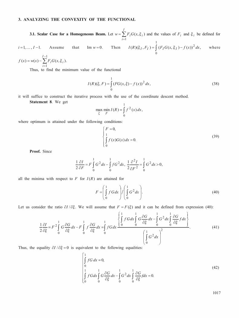
3. ANALYZING THE CONVEXITY OF THE FUNCTIONAL

3.1. Scalar Case for a Homogeneous Beam. Let w F G xi i

i

I

�

�

( , )�

1

and the values of Fi and � i be defined for

i I� �1 1, ,� . Assume that Im w � 0. Then I R F F G x f x dxI I I I( )( , ) ( ( , ) ( ))� �� ��

2

0

1

, where

f x w x F G xi i

i

I

( ) ( ) ( , )� �

�

�

�

1

1

.

Thus, to find the minimum value of the functional

I R F FG x f x dx( )( , ) ( ( , ) ( ))� �� ��

2

0

1

, (38)

it will suffice to construct the iterative process with the use of the coordinate descent method.

Statement 8. We get

max min ( ) ( )

� F

I R f x dx��

2

0

1

,

where optimum is attained under the following conditions:

F

f x G x dx

�

�

�

�

��

�

�

�

�

0

0

0

1

,

( ) ( ) .

(39)

Proof. Since

1

2

2

0

1

2

0

1

�

�

� �� �

I

FF G dx f G dx ,

1

2

0

2

2

2

0

1

�

�

� ��

I

F

G dx ,

all the minima with respect to F for I R( ) are attained for

F f Gdx G dx�

�

�

�

�

�

�

�

�

�

�

� �

0

1

2

0

1

/. (40)

Let us consider the ratio � �I / �. We will assume that F F� ( )� and it can be defined from expression (40):

1

2

2

0

1

0

1

0

1

0

1

�

�

�

�

�

�

�

�

�

�

�

�� �

�

IF G

Gdx F f

Gdx fGdx

f Gdx GG

� � �

� �

dx G dxG

f dx

G dx

0

1

2

0

1

0

1

2

0

1

2

� � �

�

�

�

�

�

�

�

��

�

�

�

��

�

�

�

�

�

. (41)

Thus, the equality � � �I / � 0 is equivalent to the following equalities:

fG dx

f Gdx GG

dx G dxG

fdx

0

1

0

1

2

0

1

0

1

0

1

0

0

�

� ���

�

�

�

�

�

�

�

�

�

,

.

� �

(42)

1017

The following relation holds:

1

2

2

2

0

0

1

2

0

1

0

1

�

��

� �

�

�

�

�

�

�

�

�

�

�

�

�

�

� �

I Gf dx G dx

fGdx� �

/

�

�

�

��

�

�

2

0.

Hence, if (40) holds, the condition fGdx F

0

1

0 0

�� �( ) guarantees that I R( ) attains minimum at point �.

Statement 9. The conditions of the Statement 8 are satisfied for an arbitrary function f x( ) for � � { }0 1, .

Proof. From (16) it follows that

f Gdx g x f x dx g x f x dx� �� ��

0

1 1

0

( , ) ( ) ( , ) ( )� �

�

�

.

Due to the continuity of g x( , )� with respect to �, the equality holds

0

0

0

�

�

��

�

�g x f x dx( , ) ( ) .

Here, g x( , )0 0� . Hence, the statement is proved.

Statement 10. Functional I R( ) has at least one minimum. All the local minima for I R( ) are defined by the

following necessary conditions:

F f Gdx G dx

F

fGdx GG

dx

�

�

�

�

�

�

�

�

�

�

�

�

�

�

�

� �

0

1

2

0

1

0

/

,

,

�

G dxG

fdx2

0

1

0

1

0

1

0

1

0

�

�

�

�

�

�

�

�

�

�

�

�

�

�

�����

(43)

and the corresponding values of

�

� are between points ��

, which are defined by the condition

f x G x dx( ( , )) ��

��

0

0

1

, (44)

and

�

( , )� � 0 1 .

Proof. According to Statement 9, when condition (40) is satisfied, there exist saddle points (minima with respect

to F and maxima with respect to �). Hence, taking into account continuous differentiability of the functional I R( ) with

respect to �, according to the Rolle theorem ( I R f dx

F

( )

,��

�

��0 1

0

2

0

1

) there exists at least one local minimum (with respect

to F and to �) for � �( , )0 1 .

If (44) holds at interior points [0, 1], then Statement 10 is true on each such interval.

The last expression in (43) is a necessary condition of the extremum I R( ) with respect to � when (40) holds.

3.2. Examples of Using the Obtained Results. Let us write the Green function by using homogeneous solutions:

G k G x x( )

( ), ( , )

4 4 4

0 1� � � �� � � ,

G G

G G

( , ) ( , ) ,

( , ) ( , ) ,

( ) ( )

0 1 0

0 1 0

2 2

� �

� �

� �

� �

�

�

�

��

where G x A nxn

n

( , ) sin� ��

�

%

1

.

1018

The boundary conditions are satisfied for an arbitrary An :

A n k nx xn

n�

%

� � �

1

4 4 4

� � � �( )sin ( ) (45)

or

1

2

1

4 4 4

A n k sn

n

sn

�

%

� �� � � �( ) sin .

Thus, As

s ks �

�

2

4 4 4

sin

( )

� �

�

,

G xn

n k

nx p n

n

n

n

( , )

sin

sin sin si�

�

� �

� � ��

�

� , �

�

%

�

%

2

4 4 4

1 1

n �nx , (46)

where p

n kn ,

�

def

2

4 4 4

� ( )

.

Let

f f nxn

n

�

�

%

1

sin � . (47)

Then condition (39) becomes

p f n nx rxdxn r

r n,

sin sin sin

�

%

�� �

1

0

1

0� � � �

or

Ff

n k

n

F

n

n

( ) sin ,

( ) .

� � �

�

�

�

�

�

�

�

�

�

�

%

4 4

1

0

(48)

From (48) it follows that minima of the functional I R( ) should be found between points ��

: F ( )��

� 0.

Let f n ns� � (i.e., f x sx( ) sin� � ). Then F

s k

s( ) sin� � ��

�

1

4 4

and �h n s�

� / , s S� 0, ,� . In this case, I R( ) has

at least S local minima.

Let us verify condition (43):

fGdx f p n

G dx p p n

n n

n

n r

n r

�

�

�

�

%

�

%

0

1

1

2

1

1

2

1

2

sin ,

sin

,

� �

� � � �

� �

�

%

�

%

�

sin sin

cos

� �� � �r p n

p p

hr n

n

n

n

n

1

2

1

4

2

2 2

1

0

1

2

1

2

� �

� �

� �

n

GG

dx G dx p h

n

n

�

%

�

�

�

��

�

�

�

��

�

�

�

�

�

�

1

2 2

1

2

1

8

2 2

,

sin n

Gfdx fGdx f p h n

n

n n

n

�

� �

�

� �

,

cos

�

%

�

%

��

�

�

�

�

�

�

1

0

1

0

1

1

0

1

2

��

�

�

�

�

�

�

�

�

�

�

�

�

�

�

�

�

�

�

�

0

1

.

(49)

1019

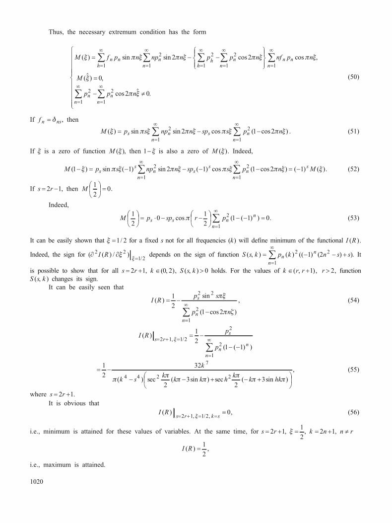
Thus, the necessary extremum condition has the form

M f p n np n p p nn n

h

n h

h

n( ) sin sin cos� � � � � �� � �

�

%

�

%

1

2 2

1

2

2 2 � � �

�

n

n n

nn

n

nf p n

M

p

�

%

�

%

�

%

�

�

�

��

�

�

�

��

�

�

1 11

2

0

cos ,

(

�

) ,

n

n

n

p n

�

%

�

%

�

�

�

�

�

��

�

�

�

�

�1

2

1

2 0cos

�

.� �

(50)

If f n ns� � , then

M p s np n sp s ps

n

n s

n

n( ) sin sin cos (� � � � � � �� � �

�

%

�

%

1

2

1

2

2 1 cos )2� �n . (51)

If � is a zero of function M ( )� , then 1� � is also a zero of M ( )� . Indeed,

M p s np n sp ss

s

n s

s

n

( ) sin ( ) sin ( ) cos1 1 2 1

2

1

� � � � �

�

%

� � � � � � � �

�

%

p nn

n

2

1

1 2( cos )� � � �( ) ( )1

sM � . (52)

If s r� �2 1, then M1

2

0

�

�

�

�

� .

Indeed,

M p sp r ps s

n

n

n1

2

0

1

2

1 1

1

2

�

�

�

�

� � � �

�

�

�

�

� � �

�

%

cos ( ( ) )� 0. (53)

It can be easily shown that � �1 2/ for a fixed s not for all frequencies (k) will define minimum of the functional I R( ).

Indeed, the sign for ( ( ) / )

/

� �

�

2 2

1 2

I R ��

depends on the sign of function S s k p k n s sn

n

n( , ) ( ) (( ) ( ) )� � � �

�

%

2

1

2

1 2 . It

is possible to show that for all s r� �2 1, k �( , )0 2 , S s k( , ) � 0 holds. For the values of k r r� �( , ),1 r � 2, function

S s k( , ) changes its sign.

It can be easily seen that

I Rp s

p n

s

n

n

( )

sin

( cos )

� �

�

�

%

1

2

1 2

2 2

2

1

��

� �

, (54)

I Rp

p

s r

s

n

n

n

( )

( ( ) )

, /� � �

�

%

� �

� �

2 1 1 2

2

2

1

1

2

1 1

�

� �

� � � � �

1

2

32

2

3

2

3

7

4 4 2 2

k

k sk

k k hk

k�

�

� �

�

�( ) ( sin ) ( ssec sec in )

,

hk��

�

�

�

(55)

where s r� �2 1.

It is obvious that

I Rs r k s

( )

, / ,� � � �

�

2 1 1 2

0

�

, (56)

i.e., minimum is attained for these values of variables. At the same time, for s r� � �2 1

1

2

, � , k n� �2 1, n r�

I R( ) �

1

2

,

i.e., maximum is attained.

1020

Let force F�

be applied at point � and force F1��

at point 1� �. In this case,

w F G x F G x� � ��� �

� �( , ) ( , )

1

1 .

From (46) it follows that

G x p n n xn

n

n

( , ) ( ) sin sin1 1

1

1

� � � ��

�

%

� �� � . (57)

Let us introduce the notation:

G xG x G x

p n nn1 2 1

1

2

2 1 2 1( , )

( , ) ( , )

sin( ) sin(�

� �

���

� �

� � � ��

) ,

( , )

( , ) ( , )

sin sin

�

�

� �

��

x

G xG x G x

p n n

n

n

�

%

�

� �

� �

1

2 2

1

2

2 2 �

� �

� �

x

F F F

F F F

n�

%

�

�

� �

� �

�

�

�

�

�

�

�

�

�

�

�

1

1 1

2 1

,

,

.

(58)

Then

I R F G F G w dx( ) ( )� � ��

0

1

1 1 2 2

2

. (59)

Conditions � � � �I F ii/ , ,0 1 2, reduce to the system of linear equations

�

�

�

��

�

�

�

�

�

� � �� �

�

,

�

} , } , {

,

K

K

� �

� �

F b

a F F bij i j

r

i i

r{ {

T T

1 1

�

,

, .

b

a G G dx b wG dx

i i

r

ij i j i i

}

�

� �� �

1

0

1

0

1

(60)

It can be easily seen that a a G G dx12 21 1

0

1

2

0� � ��

. Hence,

F wG dx G dx ii i i�

�

�

�

�

�

�

�

�

�

�

�� �

0

1

2

0

1

1 2

/, , . (61)

If w w h xh

h

�

�

1

sin � , then

F

w p n

p n

n n

n

n

n

1

2 1 2 1

1

2 1

2 2

1

2 1

2 1

�

�

�

� �

�

%

�

�

sin( )

sin ( )

��

��

%

�

�

%

�

%

�

�

�

�

�

�

�

,

sin

sin

.F

w p n

p n

n n

n

n

n

2

2 2 1

1

2

2 2

1

2

2

��

��

��

�

�

�

�

�

�

�

(62)

If wh hs� � , then for s k k N� � �2 1, , we get w n2 0� , and hence F F F2 1

0� ��

( )

� �.

In case of wh hs� � and s k k N� �2 , , we get w n2 1

0

�� and F F F

1 1

0� ��

( )

� �. The analysis is similar to that

considered above.

1021

4. RESULTS OF NUMERICAL EXPERIMENTS OF THE ANALYSIS OF MODELS

OF OPTIMAL CONTROL OF OSCILLATIONS OF THE HINGED BEAM

To determine the dependence of approximation accuracy of the given waveform on the number of forces and their

characteristics (application, amplitude and phase of oscillations), a series of numerical experiments was carried out with

the use of the multifunctional package PSG (Matlab Interface) provided by American Optimal Decision, USA [6].

Two cases were considered: oscillation of a homogeneous beam and oscillation of a beam with a defect.

4.1. Results of Modeling of Oscillation of a Homogeneous Beam. Let us present the results of numerical

solution of the problems of optimal control of oscillations of a homogeneous beam under different numbers of applied

forces and different frequencies (wave number k). The mathematical apparatus presented in Sec. 1 and the

multifunctional package PSG (Matlab Interface) were used.

As the objective function, we used root mean square deviation of the solution from the given waveform on the

frequency corresponding to the given wave number k . As is seen from Fig. 1, for any fixed frequency of oscillations,

increase in the number of applied forces reduces the approximation error. Moreover, for any fixed number of applied

forces, the approximation error increases with increase in the wave number k . For example, for any fixed number of

applied forces, approximation error corresponding to k � 1.8 is less than approximation error corresponding to greater

values of wave number k.

For wave numbers k � 1.8 and k � 4.6 and different numbers of forces, their optimal characteristics were

determined (applications, real and imaginary parts of amplitudes) that ensured the best approximation of the given form

and phase of oscillations of the homogeneous beam.

Figure 2 shows optimal characteristics of forces that correspond to wave number k � 1.8. As follows from the

figure, for any number of forces from the considered range, optimal amplitudes are regularly distributed. If the number of

applied forces does not exceed four, then the values of amplitudes are mutually commensurable. For five and more

forces, the values of the real parts of amplitudes of forces applied along beam’s edges are much greater than those for

forces applied to its interior points. The signs of imaginary parts of amplitudes (if) alternate when passing from one point

of application of forces to another. Prevailing values of imaginary parts of amplitudes correspond to extreme points of

application of forces on the beam.

Figure 3 shows optimal characteristics of forces corresponding to wave number k � 4.6. Optimal characteristics

of the forces applied to the beam for k � 4.6 substantially differ from those shown in Fig. 2 and corresponding to the case

k � 1.8. These graphs have sine curve shapes: the graph of imaginary part of amplitudes is associated with a full wave

sine curve, and the graph of real part with a semiperiodic sine curve.

1022

Fig. 1. Dependence of root mean square deviation (approximation error)

on the applied forces and frequency (wave number k ).

Number of Forces Applied

Approximation

Error(LogarithmicScale)

k � 1.8

k � 4.6

k � 4.2

k � 3.8

k � 3.4

k � 2.6

k � 2.4

k � 2.2

4.2. Results of Modeling of Oscillation of the Beam with a Defect. Let us consider the case of oscillation of

a beam with one defect, which is characterized by the following parameters: location on the beam at point �, geometrical

dimension 2� �(0, 0.1), and relative variation in the Young modulus $E. The defect can be at any section of the beam at

point � �( , )0 1 . Relative variation in the Young modulus $E can be within the interval (� 0.5, 0.5). The negative value

$E corresponds to strengthening of the cross section and positive to its weakening. The value $E � 0 means absence

of a defect. Parameter Delta E� �2 � $ is used as the characteristics of the defect.

On the assumption that all the information about defect’s parameters is known, a series of optimal control

problems for oscillations of a beam with one defect was solved for fixed values of the wave number 1.8 and four applied

forces under different values of the defect Delta and its location on the beam at point �. The mathematical apparatus

presented in Secs. 2.1 and 2.2 and the multifunctional package PSG (Matlab Interface) provided by American Optimal

Decision, USA [6] were used. As a result, for each fixed pair of values Delta and �, optimal characteristics of forces and

optimal (minimum) value of root mean square deviation (approximation error) corresponding to them were obtained.

In what follows, for simplicity, by approximation error we will mean the minimum value of approximation error obtained

as a result of solution of the optimization problem. The results are graphically presented in Figs. 4, 5. Each curve shown

in Fig. 4 describes the dependence of approximation error on the value of the defect Delta in case where the wave

number is equal to 1.8, the number of forces is four, and the unique defect on the beam is located at point �. In the case

under study, all the curves decrease on the interval � 0.05� �Delta 0 and increase on the interval 0� �Delta 0.05.

The minimum value of approximation error for all the curves equal to 1.0E�5 is attained when there are almost no

defects on the beam (| |Delta � 5.0E�6).

The behavior of the curve when the defect is located at beam’s center (� � 0.5) substantially differs from the

behavior of all other curves. In this case, the greatest value of the approximation error for Delta � � 0.05 is smaller than

for Delta � 0.05. In other cases, the greatest value of approximation error is attained for Delta � � 0.05, and the

maximum value equal to 5.2E� 4 is attained when the defect is located at point � � 0.2 or at point � � 0.8.

1023

Fig. 2. Optimal characteristics of the applied forces (application, real (rf)

and imaginary (if) parts of amplitudes) for k � 1.8: for two forces (a), three

forces (b), four forces (c), five forces (d), six forces (e), seven forces (f).

a b

dc

fe

Force Application Points Force Application Points

Amplitude

Amplitude

Amplitude

Since optimal value of the approximation error for fixed values of the parameters Delta and � corresponds to the

minimum of the objective function when the wave number is equal to 1.8, the number of forces is four, and the value of

the defect is Delta � � 0.05 and the defect is located at point � � 0.2 or at point � � 0.8, optimal value of the objective

function (approximation error) cannot be smaller than 5.2E� 4, which exceeds 52 times the optimal value of

approximation error in case of absence of defects on the beam.

Figure 5 shows four curves, each of them describing the dependence of approximation error on the value of the defect

( )Delta for a fixed location of the defect on the beam at point � � 0.2. Despite different rates of the curves, there is some

similarity. All of them attain their minimum values for Delta � 0 (when defects on the beam are absent). For any fixed value

1024

Fig. 3. Optimal characteristics of the applied forces (application, real (rf)

and imaginary (if) parts of amplitudes) for k � 4.6: for five forces (a), six

forces (b), seven forces (c), eight forces (d), nine forces (e); ten forces (f).

a b

dc

fe

Force Application Points

Force Application Points

Amplitude

Amplitude

Amplitude

Fig. 4. Dependence of approximation error on Delta for locations of the defect on

the beam � � 0.1, 0.2, 0.3, 0.4, 0.5 (a); � � 0.6, 0.7, 0.8, 0.9 (b) for the wave

number 1.8 and number of forces equal to 4.

a b

Delta

Approximation

Error

� � 0.1

� � 0.2

� � 0.4

� � 0.3

� � 0.5

� � 0.8

� � 0.6

� � 0.9

Delta

� � 0.7

of the defect (Delta ), the curve corresponding to the greater number of forces has smaller values of approximation error.

The greatest values of approximation error are shown by the curve corresponding to the least number of forces (two forces).

As follows from the results presented in Fig. 5, to reduce the optimal value of approximation error for fixed values

of Delta and �, it is necessary to increase the number of forces applied to the beam.

In Fig. 6a, we can see variation in the value of the real parts of the amplitudes as the value of the defect (Delta)

localized in the left-hand side of the beam (� � 0.4) increases from � 0.05 to 0.05. As one can see, for any value of Delta on

the interval (� 0.05, 0.05), the sign of these characteristics remains negative. The real (rf_1, rf_2) parts of the amplitudes of

forces applied to the left-hand side of the beam vary greater than respective components of the forces (rf_3, rf_4) applied

to its right-hand side. At the left end of the interval of values of the defect Delta, | | | |rf_1 rf_2� , and at the right end

| | | |rf_1 rf_2� . Here, | | | |rf_4 rf_3� for any value of Delta on the interval (� 0.05, 0.05). Hence, if the defect is located on

the left-hand part of the beam, variation in its value renders a greater influence on the forces applied on the same part of the

beam. The values of rf_1 and rf_3 increase on the intervals of variation of Delta (� 5E � 2, � 4.6E� 4) and (0, 5E� 2), and

the values of rf_2 and rf_4 decrease on these intervals. For Delta � 0, the real parts of all amplitudes attain their minimum,

which corresponds to oscillation of a defect-free beam. Figure 6b shows (in close up) variation of all the characteristics on

a small interval (� 0.001, 0.001) of the values of Delta near the minimum point.

Figure 7a shows variation in the value of imaginary parts of the amplitudes as the value of the defect (Delta)

localized in the left-hand side of the beam (� � 0.4) increases from � 0.05 to 0.05. As one can see, for any value of Delta

on the interval (� 0.05, 0.05), the sign of each characteristics does not vary. As well as in the case of no defects

(see Fig. 2), signs of imaginary parts of the amplitudes alternate when passing from one point of application of forces to

1025

Fig. 5. Dependence of approximation error on

Delta when two forces (1), four forces (2),

six forces (3), eight forces (4) are used, position

of the defect on the beam is fixed at point

� � 0.2, and wave number is 1.8.

Delta

Approximation

Error

1

2

4

3

Fig. 6. Dependence of the real parts of amplitudes of four applied forces

(rf_1, rf_2, rf_3, rf_4) on Delta for a fixed position of the defect on the beam

at point � � 0.4, wave number 1.8 in case of variation of Delta within the

limits (� 0.05, 0.05) (a), (� 0.001, 0.001) (b).

a

Delta

�140

�200

�150

�160

�170

�180

�190

Amplitude

�5.0E�2

4.5E�2

�3.9E�2

�2.9E�2

2.4E�3

�7.8E�3

�1.9E�2

1.4E�2

2.4E�2

3.4E�2

b

�185

�175

�165

�195

�155

rf_4

rf_3

rf_1

rf_2

7.3E�4

6.1E�4

.4.2E�4

�2.6E�4

�5.0E�6

2.0E�4

�5.4E�4

8.5.E�4

Delta

�9.9E�4

�7.9E�4

Amplitude

another. Imaginary parts of the amplitudes of forces (if_1, if_2) applied at points in the left-hand side of the beam vary

greater than respective components of forces (if_3, if_4) applied at points in its right-hand side. Figure 7b shows

(in close up) variation of all the characteristics on a small interval (� 0.001, 0.001) of the values of Delta.

CONCLUSIONS

We have considered the optimal control problem for oscillations of a hinged beam under the influence of external

periodic forces. We have analyzed two deterministic statements of this problem on the assumption that all the parameters

are known exactly. In the simplest statement of the problem, it is supposed that the beam structure is homogeneous.

In the more complex statement, presence of inhomogeneities (defects) on the beam is assumed. The problem is to find the

number of forces and their characteristics (application, amplitude and phase of oscillations) that ensure the required

waveform with a given accuracy. By means of analytical methods, we have reduced the problems under study to simpler

optimization problems. We have obtained analytical expressions for the objective functions and their gradients.

We have used the analytical results and carried out a series of numerical experiments in order to investigate the

dependence of the accuracy of approximation of the given waveform on the number of forces and their characteristics

(application, amplitude and phase of oscillations). We have established that in case of a homogeneous beam (no defects),

for any fixed frequency of oscillations, increase in the number of applied forces reduces the approximation error.

Moreover, for any fixed number of applied forces, the approximation error increases as wave number increases. We have

analyzed the dependences of optimal characteristics of applied forces on the number of applied forces. When modeling

the oscillation of the beam with a defect, we have analyzed the dependence of approximation error on the value of the

defect, its position on the beam, and numbers of forces applied to the beam. We have shown that for fixed parameters of

the defect, approximation error can be reduced by increasing the number of forces applied to the beam. We have also

shown that optimal characteristics of forces depend on location of the defect and parameters.

REFERENCES

1. G. M. Zrazhevsky, “Determination of the optimal parameters of the beam waveform actuation,” Bulletin of Taras

Shevchenko National University of Kyiv, Ser. Physics & Matematics, Issue 3 (2013), pp. 138–141. URL:

http://nbuv.gov.ua/ UJRN/VKNU_fiz_mat_2013_3_34.

2. L. H. Donnell, Beams, Plates, and Shells, McGraw-Hill Book Co., New York (1976).

3. S. Timoshenko and S. Woinowsky-Krieger, Theory of Plates and Shells, McGraw-Hill Book Co., New York (1959).

4. O. C. Zienkiewicz and R. L. Taylor, The Finite Element Method for Solid and Structural Mechanics,

Butterworth–Heinemann, Oxford (2005).

5. N. I. Akhiezer, Lectures on the Approximation Theory [in Russian], Nauka, Moscow (1965).

6. AORDA Portfolio Safeguard (PSG). URL: http://www.aorda.com/html/PSG_Help_HTML/index.html?bpoe.htm.

1026

Fig. 7. Dependence of the imaginary part of the amplitudes of four applied

forces (if_1, if_2, if_3, if_4) on Delta for a fixed position of a defect

on the beam at point � � 0.4, wave number 1.8 under variation of Delta

within the limits (� 0.05, 0.05) (a), (� 0.001, 0.001) (b).

a

Delta

90

�210

40

�10

�60

�110

�160

Amplitude

�5.0E�2

�3.9E�2

�2.8E�2

5.2E�3

�5.5E�3

�1.7E�2

1.7E�2

2.7E�2

3.9E�2

Amplitude

b

�55

�15

25

�95

rf_4

rf_3

rf_1

rf_2

7.3E�4

6.1E�4

.4.2E�4

�2.6E�4

�5.0E�6

2.0E�4

�5.4E�4

8.5.E�4

Delta

�9.9E�4

�7.9E�4

65