Embed Size (px)
Citation preview

Mathematical Methods for the Physical Sciences
Two Semester Course
Shawn D. Ryan, Ph.D.

Copyright c© 2015-2016 Dr. Shawn D. Ryan
PUBLISHED ONLINE
Special thanks to Mathias Legrand ([email protected]) with modifications by Vel([email protected]) for creating and modifying the template used for these lecture notes. Also,thank you to the students in the Mathematical Methods I-II class at Kent State University in the2015-2016 academic year including K. Bittinger, R. Dovishaw, T. Dubensky, M. Grose, K. Khanal,J. Krusinski, E. McMasters, J. Paltani, J. Sobieski, J. Taylor, C. Zickel, B. Zimmerman.
Licensed under the Creative Commons Attribution-NonCommercial 3.0 Unported License (the“License”). You may not use this file except in compliance with the License. You may obtain acopy of the License at http://creativecommons.org/licenses/by-nc/3.0. Unless requiredby applicable law or agreed to in writing, software distributed under the License is distributed on an“AS IS” BASIS, WITHOUT WARRANTIES OR CONDITIONS OF ANY KIND, either express or implied.See the License for the specific language governing permissions and limitations under the License.
First published online, February 2016

Contents
I Part One: Complex Numbers
1 Fundamentals of Complex Numbers . . . . . . . . . . . . . . . . . . . . . . . . . . . 11
1.1 Introduction 11
1.2 Real and Imaginary Parts of a Complex Number 14
1.3 The Complex Plane 151.3.1 Review of Unit Circle in Radians . . . . . . . . . . . . . . . . . . . . . . . . . . . . . . . . . . . . . 161.3.2 Going Deeper: Understanding Euler’s Identity . . . . . . . . . . . . . . . . . . . . . . . . . 19
1.4 Terminology and Notation 201.4.1 Complex Conjugation . . . . . . . . . . . . . . . . . . . . . . . . . . . . . . . . . . . . . . . . . . . . 22
1.5 Complex Algebra 241.5.1 Simplifying to Standard Form x+ iy . . . . . . . . . . . . . . . . . . . . . . . . . . . . . . . . . . . 241.5.2 Complex Conjugation of an Expression . . . . . . . . . . . . . . . . . . . . . . . . . . . . . . 291.5.3 Finding the Absolute Value |z| . . . . . . . . . . . . . . . . . . . . . . . . . . . . . . . . . . . . . . 301.5.4 Complex Equations . . . . . . . . . . . . . . . . . . . . . . . . . . . . . . . . . . . . . . . . . . . . . . 301.5.5 Graphs of Complex Equations . . . . . . . . . . . . . . . . . . . . . . . . . . . . . . . . . . . . . . 311.5.6 Physical Applications . . . . . . . . . . . . . . . . . . . . . . . . . . . . . . . . . . . . . . . . . . . . . 32
1.6 Complex Infinite Series 331.6.1 Review from Calculus: Tests for Convergence . . . . . . . . . . . . . . . . . . . . . . . . . . 341.6.2 Examples with Complex Series . . . . . . . . . . . . . . . . . . . . . . . . . . . . . . . . . . . . . 35
1.7 Complex Power Series and Disk of Convergence 35
1.8 Elementary Functions of Complex Numbers 37
1.9 Euler’s Formula 38
1.10 Powers and Roots of Complex Numbers 40

1.11 The Exponential and Trigonometric Functions 421.12 Hyperbolic Functions 44
II Part Two: Linear Algebra
2 Fundamentals of Linear Algebra . . . . . . . . . . . . . . . . . . . . . . . . . . . . . . . 47
2.1 Systems of Linear Equations 472.1.1 Matrix Notation . . . . . . . . . . . . . . . . . . . . . . . . . . . . . . . . . . . . . . . . . . . . . . . . . 482.1.2 Elementary Row Operations . . . . . . . . . . . . . . . . . . . . . . . . . . . . . . . . . . . . . . . 492.1.3 Fundamental Questions In Linear Algebra . . . . . . . . . . . . . . . . . . . . . . . . . . . . 49
2.2 Row Reduction and Echelon Forms 492.2.1 Solutions of Linear Systems . . . . . . . . . . . . . . . . . . . . . . . . . . . . . . . . . . . . . . . . . 50
2.3 Determinants and Cramer’s Rule 512.3.1 Special Case: Upper and Lower Triangular Matrices . . . . . . . . . . . . . . . . . . . . 532.3.2 Properties of Determinants . . . . . . . . . . . . . . . . . . . . . . . . . . . . . . . . . . . . . . . . 532.3.3 Cramer’s Rule . . . . . . . . . . . . . . . . . . . . . . . . . . . . . . . . . . . . . . . . . . . . . . . . . . 54
2.4 Vectors 552.4.1 Scalar Product . . . . . . . . . . . . . . . . . . . . . . . . . . . . . . . . . . . . . . . . . . . . . . . . . . 562.4.2 Vector (Cross) Product . . . . . . . . . . . . . . . . . . . . . . . . . . . . . . . . . . . . . . . . . . . . 572.4.3 Orthogonality . . . . . . . . . . . . . . . . . . . . . . . . . . . . . . . . . . . . . . . . . . . . . . . . . . 57
2.5 Lines, Planes, and Geometric Applications 582.6 Matrix Operations 622.6.1 Scalar Multiplication of Matrices . . . . . . . . . . . . . . . . . . . . . . . . . . . . . . . . . . . . 622.6.2 Addition and Subtraction of Matrices . . . . . . . . . . . . . . . . . . . . . . . . . . . . . . . . 622.6.3 Multiplication and Division of Matrices . . . . . . . . . . . . . . . . . . . . . . . . . . . . . . . 632.6.4 Matrix Equation . . . . . . . . . . . . . . . . . . . . . . . . . . . . . . . . . . . . . . . . . . . . . . . . . 642.6.5 Solution Sets of Linear Systems . . . . . . . . . . . . . . . . . . . . . . . . . . . . . . . . . . . . . . 642.6.6 Inverse Matrix . . . . . . . . . . . . . . . . . . . . . . . . . . . . . . . . . . . . . . . . . . . . . . . . . . . 672.6.7 Ways to Compute A−1 . . . . . . . . . . . . . . . . . . . . . . . . . . . . . . . . . . . . . . . . . . . . 672.6.8 Rotation Matrices . . . . . . . . . . . . . . . . . . . . . . . . . . . . . . . . . . . . . . . . . . . . . . . 682.6.9 Functions of Matrices . . . . . . . . . . . . . . . . . . . . . . . . . . . . . . . . . . . . . . . . . . . . . 68
2.7 Linear Combinations, Functions, and Operators 692.7.1 Linear Functions . . . . . . . . . . . . . . . . . . . . . . . . . . . . . . . . . . . . . . . . . . . . . . . . . 702.7.2 Linear Operators . . . . . . . . . . . . . . . . . . . . . . . . . . . . . . . . . . . . . . . . . . . . . . . . 71
2.8 Matrix Operations and Linear Transformations 722.9 Linear Dependence and Independence 732.9.1 Special Cases . . . . . . . . . . . . . . . . . . . . . . . . . . . . . . . . . . . . . . . . . . . . . . . . . . 742.9.2 Linear Independence of Functions . . . . . . . . . . . . . . . . . . . . . . . . . . . . . . . . . . 752.9.3 Basis Functions . . . . . . . . . . . . . . . . . . . . . . . . . . . . . . . . . . . . . . . . . . . . . . . . . . 75
2.10 Special Matrices 762.11 Eigenvalues and Eigenvectors 762.11.1 The Characteristic Equation: Finding Eigenvalues . . . . . . . . . . . . . . . . . . . . . . . 772.11.2 Similarity . . . . . . . . . . . . . . . . . . . . . . . . . . . . . . . . . . . . . . . . . . . . . . . . . . . . . . . 78
2.12 Diagonalization 792.12.1 Physical Interpretation of Eigenvalues, Eigenvectors, and Diagonalization . . . 83

III Part Three: Multivariable Calculus
3 Partial Differentiation . . . . . . . . . . . . . . . . . . . . . . . . . . . . . . . . . . . . . . . . . . 87
3.1 Introduction and Notation 873.1.1 Review of Product, Quotient, and Chain Rule . . . . . . . . . . . . . . . . . . . . . . . . . . 88
3.2 Power Series in Two Variables 903.3 Total Differentials 923.4 Approximations Using Differentials 933.5 Chain Rule or Differentiating a Function of a Function 953.6 Implicit Differentiation 973.7 More Chain Rule 993.7.1 Using Cramer’s Rule . . . . . . . . . . . . . . . . . . . . . . . . . . . . . . . . . . . . . . . . . . . . . 100
3.8 Maximum and Minimum Problems with Constraints 1013.9 Lagrange Multipliers 105
4 Multivariable Integration and Applications . . . . . . . . . . . . . . . . . . . . 111
4.1 Introduction 1114.2 Double Integrals Over General Regions 1144.2.1 Integrals Over Subregions . . . . . . . . . . . . . . . . . . . . . . . . . . . . . . . . . . . . . . . . 1174.2.2 Area Between Curves . . . . . . . . . . . . . . . . . . . . . . . . . . . . . . . . . . . . . . . . . . . 118
4.3 Triple Integrals 1184.3.1 Volume Between Surfaces . . . . . . . . . . . . . . . . . . . . . . . . . . . . . . . . . . . . . . . . 120
4.4 Applications of Integration 1204.4.1 Mass . . . . . . . . . . . . . . . . . . . . . . . . . . . . . . . . . . . . . . . . . . . . . . . . . . . . . . . . . 1204.4.2 Moments and Center of Mass . . . . . . . . . . . . . . . . . . . . . . . . . . . . . . . . . . . . . 1214.4.3 Moment of Inertia . . . . . . . . . . . . . . . . . . . . . . . . . . . . . . . . . . . . . . . . . . . . . . 1224.4.4 Generalization of Physical Quantities to 3D . . . . . . . . . . . . . . . . . . . . . . . . . . . 1234.4.5 Applications to Probability . . . . . . . . . . . . . . . . . . . . . . . . . . . . . . . . . . . . . . . . 123
4.5 Change of Variables in Integrals 1254.5.1 Changing to Polar Coordinates in a Double Integral . . . . . . . . . . . . . . . . . . . 1264.5.2 Arc Length in Polar Coordinates . . . . . . . . . . . . . . . . . . . . . . . . . . . . . . . . . . . 128
4.6 Cylindrical Coordinates 1284.7 Cylindrical Coordinates 1294.7.1 Jacobians . . . . . . . . . . . . . . . . . . . . . . . . . . . . . . . . . . . . . . . . . . . . . . . . . . . . 131
4.8 Surface Integrals 132
5 Vector Analysis . . . . . . . . . . . . . . . . . . . . . . . . . . . . . . . . . . . . . . . . . . . . . . 135
5.1 Applications of Vector Multiplication 1355.1.1 Dot and Cross Products . . . . . . . . . . . . . . . . . . . . . . . . . . . . . . . . . . . . . . . . . . 136
5.2 Triple Products 1375.2.1 Triple Scalar Product . . . . . . . . . . . . . . . . . . . . . . . . . . . . . . . . . . . . . . . . . . . . 1375.2.2 Triple Vector Product . . . . . . . . . . . . . . . . . . . . . . . . . . . . . . . . . . . . . . . . . . . . 1395.2.3 Applications of Triple Scalar Products . . . . . . . . . . . . . . . . . . . . . . . . . . . . . . . 1395.2.4 Application of Triple Vector Product . . . . . . . . . . . . . . . . . . . . . . . . . . . . . . . . 140

5.3 Fields 1405.4 Differentiation of Vectors 1435.4.1 Differentiation in Polar Coordinates . . . . . . . . . . . . . . . . . . . . . . . . . . . . . . . . . 144
5.5 Directional Derivative and Gradient 1455.5.1 Gradients in Other Coordinate Systems . . . . . . . . . . . . . . . . . . . . . . . . . . . . . 1475.5.2 Physical Significance . . . . . . . . . . . . . . . . . . . . . . . . . . . . . . . . . . . . . . . . . . . . 147
5.6 Some Other Expressions Involving ∇ 1485.6.1 Divergence, ∇ ·V . . . . . . . . . . . . . . . . . . . . . . . . . . . . . . . . . . . . . . . . . . . . . . . 1485.6.2 Physical Interpretation . . . . . . . . . . . . . . . . . . . . . . . . . . . . . . . . . . . . . . . . . . . 1495.6.3 Curl ∇×V . . . . . . . . . . . . . . . . . . . . . . . . . . . . . . . . . . . . . . . . . . . . . . . . . . . . . 1495.6.4 Solenoidal and Irrotational . . . . . . . . . . . . . . . . . . . . . . . . . . . . . . . . . . . . . . . 1515.6.5 Divergence and Laplacian in Other Coordinate Systems . . . . . . . . . . . . . . . . 152
5.7 Line Integrals 1525.7.1 Potentials . . . . . . . . . . . . . . . . . . . . . . . . . . . . . . . . . . . . . . . . . . . . . . . . . . . . . 1555.7.2 Alternate Approach to Finding Scalar Potential φ . . . . . . . . . . . . . . . . . . . . . . 156
5.8 Green’s Theorem in the Plane 1565.9 The Divergence (Gauss) Theorem 1605.9.1 Gauss Law for Electricity . . . . . . . . . . . . . . . . . . . . . . . . . . . . . . . . . . . . . . . . . 162
5.10 The Stokes (Curl) Theorem 1625.10.1 Ampere’s Law . . . . . . . . . . . . . . . . . . . . . . . . . . . . . . . . . . . . . . . . . . . . . . . . . 1645.10.2 Conservative Fields . . . . . . . . . . . . . . . . . . . . . . . . . . . . . . . . . . . . . . . . . . . . . 164
IV Part Four: Ordinary Differential Equations
6 Ordinary Differential Equations . . . . . . . . . . . . . . . . . . . . . . . . . . . . . . . 169
6.1 Introduction to ODEs 1696.1.1 Some Basic Mathematical Models; Direction Fields . . . . . . . . . . . . . . . . . . . . 1696.1.2 Solutions of Some Differential Equations . . . . . . . . . . . . . . . . . . . . . . . . . . . . . 1726.1.3 Classifications of Differential Equations . . . . . . . . . . . . . . . . . . . . . . . . . . . . . . 173
6.2 Separable Equations 1756.3 Linear First-Order Equations, Method of Integrating Factors 1786.3.1 REVIEW: Integration By Parts . . . . . . . . . . . . . . . . . . . . . . . . . . . . . . . . . . . . . . 1806.3.2 Modeling With First Order Equations . . . . . . . . . . . . . . . . . . . . . . . . . . . . . . . . 181
6.4 Existence and Uniqueness 1876.4.1 Linear Equations . . . . . . . . . . . . . . . . . . . . . . . . . . . . . . . . . . . . . . . . . . . . . . . . 1886.4.2 Nonlinear Equations . . . . . . . . . . . . . . . . . . . . . . . . . . . . . . . . . . . . . . . . . . . . . 189
6.5 Other Methods for First-Order Equations 1906.5.1 Autonomous Equations with Population Dynamics . . . . . . . . . . . . . . . . . . . . . 1906.5.2 Bernoulli Equations . . . . . . . . . . . . . . . . . . . . . . . . . . . . . . . . . . . . . . . . . . . . . . 1936.5.3 Exact Equations . . . . . . . . . . . . . . . . . . . . . . . . . . . . . . . . . . . . . . . . . . . . . . . . 1936.5.4 Homogeneous Equations . . . . . . . . . . . . . . . . . . . . . . . . . . . . . . . . . . . . . . . . 198
6.6 Second-Order Linear Equations with Constant Coefficients and Zero Right-Hand Side 198
6.6.1 Basic Concepts . . . . . . . . . . . . . . . . . . . . . . . . . . . . . . . . . . . . . . . . . . . . . . . . 1986.6.2 Homogeneous Equations With Constant Coefficients . . . . . . . . . . . . . . . . . . . 200

6.7 Complex Roots of the Characteristic Equation 2006.7.1 Review Real, Distinct Roots . . . . . . . . . . . . . . . . . . . . . . . . . . . . . . . . . . . . . . . 2006.7.2 Complex Roots . . . . . . . . . . . . . . . . . . . . . . . . . . . . . . . . . . . . . . . . . . . . . . . . 201
6.8 Repeated Roots of the Characteristic Equation and Reduction of Order 2046.8.1 Repeated Roots . . . . . . . . . . . . . . . . . . . . . . . . . . . . . . . . . . . . . . . . . . . . . . . . 2046.8.2 Reduction of Order . . . . . . . . . . . . . . . . . . . . . . . . . . . . . . . . . . . . . . . . . . . . . 207
6.9 Second-Order Linear Equations with Constant Coefficients and Non-zeroRight-Hand Side 209
6.9.1 Nonhomogeneous Equations . . . . . . . . . . . . . . . . . . . . . . . . . . . . . . . . . . . . . 2096.9.2 Undetermined Coefficients . . . . . . . . . . . . . . . . . . . . . . . . . . . . . . . . . . . . . . . 2106.9.3 The Basic Functions . . . . . . . . . . . . . . . . . . . . . . . . . . . . . . . . . . . . . . . . . . . . . 2106.9.4 Products . . . . . . . . . . . . . . . . . . . . . . . . . . . . . . . . . . . . . . . . . . . . . . . . . . . . . . 2136.9.5 Sums . . . . . . . . . . . . . . . . . . . . . . . . . . . . . . . . . . . . . . . . . . . . . . . . . . . . . . . . . 2156.9.6 Method of Undetermined Coefficients . . . . . . . . . . . . . . . . . . . . . . . . . . . . . . 218
6.10 Mechanical and Electrical Vibrations 2196.10.1 Applications . . . . . . . . . . . . . . . . . . . . . . . . . . . . . . . . . . . . . . . . . . . . . . . . . . . 2196.10.2 Free, Undamped Motion . . . . . . . . . . . . . . . . . . . . . . . . . . . . . . . . . . . . . . . . . 2216.10.3 Free, Damped Motion . . . . . . . . . . . . . . . . . . . . . . . . . . . . . . . . . . . . . . . . . . . 2246.10.4 Forced Vibrations . . . . . . . . . . . . . . . . . . . . . . . . . . . . . . . . . . . . . . . . . . . . . . . 227
6.11 Two-Point Boundary Value Problems and Eigenfunctions 2316.11.1 Boundary Conditions . . . . . . . . . . . . . . . . . . . . . . . . . . . . . . . . . . . . . . . . . . . . 2316.11.2 Eigenvalue Problems . . . . . . . . . . . . . . . . . . . . . . . . . . . . . . . . . . . . . . . . . . . . 233
6.12 Systems of Differential Equations 235
6.13 Homogeneous Linear Systems with Constant Coefficients 2366.13.1 The Phase Plane . . . . . . . . . . . . . . . . . . . . . . . . . . . . . . . . . . . . . . . . . . . . . . . 2376.13.2 Real, Distinct Eigenvalues . . . . . . . . . . . . . . . . . . . . . . . . . . . . . . . . . . . . . . . . 237
V Part Five: PDEs and Fourier Series
7 Fourier Series and Transforms . . . . . . . . . . . . . . . . . . . . . . . . . . . . . . . . . 247
7.1 Introduction to Fourier Series 2477.1.1 Simple Harmonic Motion . . . . . . . . . . . . . . . . . . . . . . . . . . . . . . . . . . . . . . . . . 247
7.2 Fourier Coefficients 249
7.3 Fourier Coefficients 2497.3.1 A Basic Example . . . . . . . . . . . . . . . . . . . . . . . . . . . . . . . . . . . . . . . . . . . . . . . 2517.3.2 Derivation of Euler Formulas . . . . . . . . . . . . . . . . . . . . . . . . . . . . . . . . . . . . . . . 252
7.4 Dirichlet Conditions 255
7.5 Convergence and Sum of a Fourier series 2557.5.1 Gibbs Phenomenon . . . . . . . . . . . . . . . . . . . . . . . . . . . . . . . . . . . . . . . . . . . . . 257
7.6 Complex Form of Fourier Series 257
7.7 Complex Fourier Series 2577.7.1 General Complex Fourier Series for Intervals (0,L) . . . . . . . . . . . . . . . . . . . . . . 259

7.8 General Fourier Series for Functions of Any Period p = 2L 2607.9 Even and Odd Functions 2657.10 Even and Odd Functions, Half-Range Expansions 2657.10.1 Half-Range Expansions . . . . . . . . . . . . . . . . . . . . . . . . . . . . . . . . . . . . . . . . . . 2687.10.2 Fourier Sine Series . . . . . . . . . . . . . . . . . . . . . . . . . . . . . . . . . . . . . . . . . . . . . . . 2697.10.3 Fourier Cosine Series . . . . . . . . . . . . . . . . . . . . . . . . . . . . . . . . . . . . . . . . . . . . 272
8 Partial Differential Equations . . . . . . . . . . . . . . . . . . . . . . . . . . . . . . . . . . 275
8.1 Introduction to Basic Classes of PDEs 2758.2 Introduction to PDEs 2758.2.1 Basics of Partial Differential Equations . . . . . . . . . . . . . . . . . . . . . . . . . . . . . . . 2758.2.2 Laplace’s Equation - Type: Elliptical . . . . . . . . . . . . . . . . . . . . . . . . . . . . . . . . 2768.2.3 Poisson’s Equation . . . . . . . . . . . . . . . . . . . . . . . . . . . . . . . . . . . . . . . . . . . . . . 2768.2.4 Diffusion/Heat Equation - Type: Parabolic . . . . . . . . . . . . . . . . . . . . . . . . . . . . 2768.2.5 Wave Equation - Type: Hyperbolic . . . . . . . . . . . . . . . . . . . . . . . . . . . . . . . . . 2768.2.6 Helmholtz Equation . . . . . . . . . . . . . . . . . . . . . . . . . . . . . . . . . . . . . . . . . . . . . 2768.2.7 Schrödinger Equation . . . . . . . . . . . . . . . . . . . . . . . . . . . . . . . . . . . . . . . . . . . 2768.2.8 Solutions to PDEs . . . . . . . . . . . . . . . . . . . . . . . . . . . . . . . . . . . . . . . . . . . . . . . 277
8.3 Laplace’s Equations and Steady State Temperature Problems 2778.3.1 Dirichlet Problem for a Rectangle . . . . . . . . . . . . . . . . . . . . . . . . . . . . . . . . . . 2788.3.2 Dirichlet Problem For A Circle . . . . . . . . . . . . . . . . . . . . . . . . . . . . . . . . . . . . . 279
8.4 Heat Equation and Schrödinger Equation 2818.4.1 Derivation of the Heat Equation . . . . . . . . . . . . . . . . . . . . . . . . . . . . . . . . . . . 282
8.5 Separation of Variables and Heat Equation IVPs 2838.5.1 Initial Value Problems . . . . . . . . . . . . . . . . . . . . . . . . . . . . . . . . . . . . . . . . . . . . 2838.5.2 Separation of Variables . . . . . . . . . . . . . . . . . . . . . . . . . . . . . . . . . . . . . . . . . . 2848.5.3 Neumann Boundary Conditions . . . . . . . . . . . . . . . . . . . . . . . . . . . . . . . . . . . 2868.5.4 Other Boundary Conditions . . . . . . . . . . . . . . . . . . . . . . . . . . . . . . . . . . . . . . . 287
8.6 Heat Equation Problems 2878.6.1 Examples . . . . . . . . . . . . . . . . . . . . . . . . . . . . . . . . . . . . . . . . . . . . . . . . . . . . . 289
8.7 Other Boundary Conditions 2918.7.1 Mixed Homogeneous Boundary Conditions . . . . . . . . . . . . . . . . . . . . . . . . . . 2918.7.2 Nonhomogeneous Dirichlet Conditions . . . . . . . . . . . . . . . . . . . . . . . . . . . . . 2928.7.3 Other Boundary Conditions . . . . . . . . . . . . . . . . . . . . . . . . . . . . . . . . . . . . . . . 295
8.8 The Schrödinger Equation 2958.9 Wave Equations and the Vibrating String 2968.9.1 Derivation of the Wave Equation . . . . . . . . . . . . . . . . . . . . . . . . . . . . . . . . . . 2968.9.2 The Homogeneous Dirichlet Problem . . . . . . . . . . . . . . . . . . . . . . . . . . . . . . . 2978.9.3 Examples . . . . . . . . . . . . . . . . . . . . . . . . . . . . . . . . . . . . . . . . . . . . . . . . . . . . . 2998.9.4 D’Alembert’s Solution of the Wave Equation, Characteristics . . . . . . . . . . . . 300
Index . . . . . . . . . . . . . . . . . . . . . . . . . . . . . . . . . . . . . . . . . . . . . . . . . . . . . . . 303

I
1 Fundamentals of Complex Numbers . . 111.1 Introduction1.2 Real and Imaginary Parts of a Complex Number1.3 The Complex Plane1.4 Terminology and Notation1.5 Complex Algebra1.6 Complex Infinite Series1.7 Complex Power Series and Disk of Convergence1.8 Elementary Functions of Complex Numbers1.9 Euler’s Formula1.10 Powers and Roots of Complex Numbers1.11 The Exponential and Trigonometric Functions1.12 Hyperbolic Functions
Part One: Complex Numbers


1. Fundamentals of Complex Numbers
1.1 Introduction
The two course sequence Mathematical Methods in the Physical Sciences I and II are designed tocondense many courses in higher level mathematics into the essential information needed to studyupper level physics undergraduate courses. Our main focus is to develop mathematical intuition forsolving real world problems while developing our tool box of useful methods. Topics in this courseare derived from five principle subjects in Mathematics
(i) Complex Numbers (Math 42048, Boas Ch. 2)→ Quantum Mechanics
(ii) Linear Algebra (Math 21001, Boas Ch. 3) → Transformations, Change of Coor.,Stability
(iii) Multivariable Calculus (Math 22005, Boas Ch. 4-6)→ Forces, Inertia, Volume, Area
(iv) Introduction to Ordinary Differential Equations (Math 32044, Boas Ch. 7-8) →Particle Motion, Dynamics
(v) Introduction to Partial Differential Equations (Math 42045, Boas Ch. 13)→ SignalAnalysis, Heat Conduction, Waves, Equilibrium Physics
Each class individually goes deeper into the subject, but we will cover the basic tools needed tohandle problems arising in physics, materials sciences, and the life sciences. Your upper levelcurses will introduce the physical motivation for the problems, but here we will develop the solutionmethods for solving those problems. In Math Methods 1 we will cover Chapters 2 - 5 or the firsthalf of our list.
Recall the first place you most likely saw a complex number: solving a quadratic equationax2 +bx+ c = 0 with the quadratic formula
x =−b±
√b2−4ac
2a.

12 Chapter 1. Fundamentals of Complex Numbers
When the so-called discriminant, b2− 4ac is negative the square root produces an imaginarynumber. For example if one wants to solve x2 +1 = 0 the quadratic formula gives ±
√(−1) =±i.
A quadratic equation must have two roots or solutions and the imaginary number i was introducedto handle such cases.
Consider some easy examples for how to handle negative square roots.
Example 1.1 i)√−64 = 8
√−1 = 8i
ii)√−5 =
√5√−1 =
√5i
iii) Powers of i: i =√−1, i2 =
√−1√−1 =−1, i3 = i2i =−i, i4 = i2i2 = 1. Any other power of i
can be found by dividing the exponent by 4 and only considering the remainder i53 = i4(13)i1 = i.
Just as a refresher solve the following quadratic equation using the quadratic formula
Example 1.2 Solve x2− x+1 = 0. The quadratic formula gives
x =1±√
1−42
=1±√−3
2=
12±√
32
i
We have this built up intuition from the past, but what exactly is a complex number. Let’smake an analogy with negative numbers (thanks Kalid Azad for the insight). Imagine a time beforenegative numbers were accepted around the 1700’s in Europe. Given two numbers 7 and 8 we caneasily write 8−7 = 1. Starting with 8 sheep, if I give you 7 I will only have one left. What about7−8? How can I have less than nothing? The problem is trying to think about this problem withconcrete objects. The easiest way to understand this is with money. If I owe you $50 and I am paidonly $10 to teach this course, then at the end of the day I have lost $40 hence the negative sign. Inthis case −40 represents a debt or something I owe. The negative sign was invented to keep trackof which direction I am (positive I earned money or negative I owe money).
Figure 1.1: Thanks to Kalid Azad for the figures
Now, how to we handle a square root of a number less than zero? Suppose we want to solvex2 = 9. This mean finding a number such that 1× x× x = 9. What can I apply to 1 twice so that Ireceive 9? The answers are 3 and −3. We can scale 1 by 3 and then scale by 3 again or we canscale 1 by negative 3 (scale by 3 and reflect it to negative side) and do the same again.
Now, try to solve x2 =−1, or 1× x× x =−1. What can we apply twice to turn 1 into -1? Wecannot multiply by a positive or negative number twice, because the result will be negative. What ifwe rotated it by 90 (see Figure‘1.1)? This works, but what does it mean. Summary:

1.1 Introduction 13
Figure 1.2: Thanks to Kalid Azad for the figures
1) i can be thought of as a “new dimension" to measure a number
2) Multiplying by i is a rotation of a number by 90 counter-clockwise
3) Multiplying by −i is a rotation of a number by 90 clockwise
Complex numbers are very similar to real numbers. Can we make sense of arithmetic operationsof complex number (e.g., +,−,×,÷)? What about functions of complex numbers such as ei orsin(iz) and cos(iz)?. Also, in the upcoming sections we will consider graphing, power series ofcomplex functions/radius of convergence, and distances or magnitudes of complex numbers.

14 Chapter 1. Fundamentals of Complex Numbers
1.2 Real and Imaginary Parts of a Complex NumberSo according to the last section numbers can be two-dimensional! Can a number be both real andimaginary? YES! Take for example the solution to x2− x+ 1
2 = 0, which is 1+ i. This number hasboth a real part 1 and a purely imaginary part i, but together they form a complex number of theform x+ yi.
Definition 1.2.1 A complex number is any number of the form z = x+ iy where x and y arereal numbers. x is called the real part and y is called the imaginary part.
R Notice the imaginary part y of a complex number z = x+ iy is in fact real! It is the realnumber coefficient for i.
Example 1.3 Find the real and imaginary parts of:
i) 5+6i, Re5+6i= 5 and Im5+6i= 6.
ii) −1+3i, Re−1+3i=−1 and Im−1+3i= 3.
iii) 6i, Re6i= 0 and Im6i= 6.
iii) 7, Re7= 7 and Im7= 0.
All real numbers are complex numbers with zero imaginary part. Therefore the real numbersare a subset of the complex numbers; however, there is a more useful observation. All complexnumbers can be written as z = x+ yi. If we associate this with the point (x,y) in two-dimensionalspace, then we can plot complex numbers (see Figure 1.3.2). In the next section we will investigategraphing complex numbers further.
Figure 1.3: Thanks to Kalid Azad for the figures

1.3 The Complex Plane 15
1.3 The Complex PlaneAs mentioned briefly before, the two-dimensional real space can be thought of as equivalentto the complex plane, R2 ' C. Any complex number can be associated to a point we can plotin the xy-plane with a traditional Cartesian coordinate system. Consider the complex numberz = 2+3i→ (2,3)
x
y
(2,3)•
Example 1.4 Plot 4+3i, 3i, 5, -1-i
x
y
(4,3)•(0,3)•
(5,0)•
(−1,−1)•
Recall from calculus another form on coordinates in two dimensions, polar coordinates(x,y) 7→ (r,θ). Can we use the same idea to identify complex numbers with their associatedpolar coordinates? Yes!
Definition 1.3.1 (Polar Coordinates of Complex Numbers) Any complex number z = x+ iy canbe written in polar form using the same relations from two dimensional Cartesian coordinates
r =√
x2 + y2
θ = tan−1(y/x)
or
x = r cos(θ)
y = r sin(θ).
Thus, z = x+ iy = rcos(θ)+ isin(θ) = r [cos(θ)+ isin(θ)]. NOTE: That all the quantitiesinvolved are real (e.g., x,y,r,θ )!

16 Chapter 1. Fundamentals of Complex Numbers
x
y
(x,y)
θ
r
x
y
•
We can actually simplify this expression further with the help of Euler’s Identity
Definition 1.3.2 (Euler’s Identity) The polar form of a complex number can be written as
eiθ = cos(θ)+ isin(θ). (1.1)
This will be taken as a fact for now and will be shown explicitly in a few sections when we studycomplex power series.
R Traditionally if asked for the polar form of a complex number z the expectation is that it iswritten z = reiθ .
Key idea: For solving a lot of problems with complex numbers the main task is to identifywhether it would be easier to tackle the problem in Cartesian (x,y) or polar (r,θ) coordinates.
1.3.1 Review of Unit Circle in Radians
You need to be very familiar with the standard right triangles, 45-45-90 and 30-60-90 in eachquadrant in order to effectively use the polar form of a complex number. Even though the unitcircle is familiar we must also be able to scale to any size right triangle of these two forms.

1.3 The Complex Plane 17
x
y
0
30
6090
120
150
180
210
240270
300
330
360
π
6
π
4
π
3
π
22π
33π
4
5π
6
π
7π
6
5π
44π
33π
2
5π
3
7π
4
11π
6
2π
(√3
2 , 12
)(√
22 ,√
22
)(
12 ,√
32
)
(−√
32 , 1
2
)(−√
22 ,√
22
)(−1
2 ,√
32
)
(−√
32 ,−1
2
)(−√
22 ,−
√2
2
)(−1
2 ,−√
32
)
(√3
2 ,−12
)(√
22 ,−
√2
2
)(
12 ,−
√3
2
)
(−1,0) (1,0)
(0,−1)
(0,1)
Example 1.5 For each of the following find the polar form and plot the result in two-dimensions.
i) z =−1+√
3i
Step 1: Find r =√
x2 + y2 =√
1+3 = 2.
Step 2: Find θ = tan−1(√
3/1). Recall that tangent is opposite over adjacent. Thus, we needa triangle where the opposite side has length
√3 and the adjacent side is along -1. If x < 0 and
y > 0 we are in quadrant II with a 30-60-90 right triangle. Therefore θ = 2π
3 .
Step 3: Write in polar form z = 2ei 2π
3 .
Step 4: Plot the result!

18 Chapter 1. Fundamentals of Complex Numbers
x
y(−1,
√3)
r
•
θ
ii) z = 1− i
Step 1: Find r =√
x2 + y2 =√
1+1 =√
2.
Step 2: Find θ = tan−1(−1/1). The tangent is opposite over adjacent. Thus, we need a tri-angle where the opposite side is along -1 and the adjacent side is along 1. If x > 0 and y < 0 we arein quadrant IV with a 45-45-90 right triangle. Therefore θ = 3π
4 or −π
4 . Note that it is important toobserve the sign of both x and y to be in the correct quadrant.
Step 3: Write in polar form z =√
2ei 7π
4 .
Step 4: Plot the result!
x
y
(−1,1)
r •
θ
iii) z = 3i
Step 1: Find r =√
x2 + y2 =√
0+9 = 3.
Step 2: Find θ = tan−1(5/0). We are looking for an angle whose tangent is ∞. Recall thattangent is sine over cosine. the tangent is infinite if cos(θ) = 0 or θ = π/2 or θ =−π/2. Sincey > 0, then θ = π/2.

1.3 The Complex Plane 19
Step 3: Write in polar form z = 3ei π
2 .
Step 4: Plot the result!
x
y
(0,3)•
θ
1.3.2 Going Deeper: Understanding Euler’s Identity
Figure 1.4: Thanks to Kalid Azad for the figures.
20 Chapter 1. Fundamentals of Complex Numbers
Euler’s Identity eiθ = cos(θ)+ isin(θ) is a formula, which explains how to move around theunit circle. Consider a point confined to the unit circle traveling x radians. The horizontal distancetraveled is cos(x) and the vertical distance traveled is sin(x). To take these two coordinates andcombine them into one number we make it complex! z = cos(x)+ isin(y). Thus, the right side ofEuler’s formula/identity describes motion on a circle.
The left-hand side of Euler’s Identity contains the exponential function e. In real number thefunction ex arises in problems involving growth or decay at a fast rate. Here what do we meanby imaginary growth (eiθ )?!? Imaginary growth is different than normal exponential growth. Thegrowth is in a different direction, instead of going forward we growth along the imaginary axis(y-direction or 90). Instead of speeding up or slowing down a point begins to rotate (multiplying anumber by i does not change its magnitude it only rotates it).
Figure 1.5: Thanks to Kalid Azad for the figures.
Thinking Question In real numbers the exponential function keeps growing larger and larger,so in the case of “imaginary growth" should we rotate faster and faster?
Since we are constrained to the unit circle instead of growing larger and larger, a point movesfurther along the circle. For example if we compare eiθ and e2iθ . The magnitude does not change(still 1), but we rotate twice as far (or travel twice as long if θ is thought of as time).
Interesting Case: Complex Growth What if the growth rate is complex ex+iy?
The real part ex grows like normal while the imaginary part eiy rotates. Thus, one can expecta spiral shape. This will be seen later when finding complex solutions to equations of motion!!
1.4 Terminology and NotationIn this class we will always use i to denote the complex (pure imaginary) number i :=
√−1. Be
aware that in many physics textbooks j is also used. Often this is seen when studying electricitywhere current is denoted as i to avoid confusion. An additional point regarding notation is that acomplex number z = x+ iy is one number so when labeling points in the complex plane usually asingle letter is used (e.g., A,B,P etc.).
Recall from the last lecture the polar from of a complex number using Euler’s identity.
z = x+ iy = r(cos(θ)+ isin(θ) = reiθ (1.2)

1.4 Terminology and Notation 21
Figure 1.6: Thanks to Kalid Azad for the figures.
where the real part of z, Rez = x, and the imaginary part of z, Imz = y. In addition, themagnitude or length associated with the complex number z is r = |z| =
√x2 + y2 and the angle
θ = tan−1(y/x).
Example 1.6 Write z =−√
3−3i in polar form and plot it.
Step 1: Find r =√
x2 + y2 =√
3+9 = 2√
3.
Step 2: Find θ = tan−1(−3/−√
3) = tan−1(−√
3/− 1). Recall that tangent is opposite overadjacent. Thus, we need a triangle where the opposite side along −
√3 and the adjacent side is
along -1. If x < 0 and y < 0 we are in quadrant III with a 30-60-90 right triangle. Therefore θ = 4π
3 .
Step 3: Write in polar form z = 2√
3ei 4π
3 .
Step 4: Plot the result!

22 Chapter 1. Fundamentals of Complex Numbers
x
y
(−√
3,−3)
θre f
r
•
θ
Note that due to periodicity the true answer for the angle is θ = 4π
3 +2πn where n is an integer.The first component, θprinciple := 4π
3 , is known as the principle angle and must be between thestandard interval of 0≤ θp < 2π . Another angle of importance is the reference angle, 0≤ θre f ≤ π
2 ,which gives the magnitudes of the sides of the 30-60-90 or 45-45-90 right triangle. Observe that thereference angle has nothing to do with the sign of each side of the triangle, because it is independentof the quadrant it is in.
Figure 1.7: Difference between principle angle θp (black) and the reference angle θre f (red).
R When working with complex numbers make sure that the angle θ you find is in the samequadrant as the complex number itself.
1.4.1 Complex ConjugationConsider two complex numbers z1 = x+ iy and z2 = x− iy. The only difference is the sign of theimaginary part, ±iy. These two complex numbers are known as complex conjugates. Specifically,z2 is the complex conjugate of z1 denoted by z2 = z1. Where the bar indicates “complex conjugate"(in some textbooks the notation of a ? is used, z2 = z?1. Given any complex number we can alwaysfind its conjugate by changing the sign of the imaginary part. You may have come across these pairs

1.4 Terminology and Notation 23
before when solving quadratic equations, because complex solutions to equations always come asconjugate pairs. In other words, if z = 2+3i is a solution, then z = 2−3i must also be a solution.
Example 1.7 Find the complex conjugate of each of the following complex numbers:
i) z = 1+ i, then z = 1− i
ii) z =−2−4i, then z =−3+4i
iii) z =−5i, then z = 5i
iv) z =−3, then z =−3
v) z = 0, then z = 0
It is easy to blindly remember to change the sign of the imaginary part, but let’s look at a pairof complex conjugates plotted on the same coordinate plane to see if there is any relationship. Letslook back at Example 3 i) and ii) .
x
y
(1,1)
(1,−1)
(−2,−4)
(−2,4)
•
•
•
•
The complex conjugate of a number is just its reflection across the x-axis (real axis).
Thinking Question: A complex conjugate is just a reflection across the x-axis so the changein (x,y) coordinates is simple y 7→ −y. How does a complex conjugate effect the polar form of acomplex number?
Answer: The magnitude of a complex number and its conjugate are identical so r remains the same.However, θ 7→ −θ . What does this mean in terms of the principle angle and the reference angle?The reference angle θre f remains unchanged, but the principle angle changes sign. So if θ = π
4 ,then θz =−π
4 or 7π
4 .

24 Chapter 1. Fundamentals of Complex Numbers
We can also directly see this from the polar form of a complex number
z= x+ iy= r [cos(θ)+ isin(θ)] = r [cos(−θ)+ isin(−θ)] = r [cos(θ)− isin(θ)] = x− iy. (1.3)
1.5 Complex Algebra
With real numbers we can perform various algebraic operations to combine them into somethingnew. These include, but are not limited to
i) Basic Operations: Addition +, Subtraction −, Multiplication ×, and Division ÷
ii) Magnitude and Distance | · |, v = |v|, or |a−b|.
iii) Solving Equations 4x = 6
Now we will consider the complex analogue of each of these as well as some physical applicationsfor complex numbers.
1.5.1 Simplifying to Standard Form x+ iy
As we have seen before complex numbers can be written in two equivalent forms z = x+ iy = reiθ .The first form is referred to as standard form and will be useful for the basic operations.
Addition of Complex Numbers
Definition 1.5.1 Given two complex numbers z1 = x1 + iy1 and z2 = x2 + iy2, their sum z1 + z2is defined as
(x1 + iy1)+(x2 + iy2) = (x1 + x2)+ i(y1 + y2) (1.4)
Just add the real parts and add the imaginary parts.
Example 1.8 i) (1+ i)+(2−3i) = (1+2)+ i(1+(−3)) = 3−2i
ii) (1+5i)+(−4i) = (1+0)+ i(5+(−4)) = 1+ i
iii) (1+0i)+(0+2i) = (1+0)+ i(0+2) = 1+2i
Now, let’s visualize Example 2i).

1.5 Complex Algebra 25
x
y
z1
z1 + z2
z2
z2 + z1
z1 + z2
This visualization shows two key ideas:
1. The addition of complex numbers behaves exactly as vector addition in two-dimensions (recallthe analogy between R2 ∼= C).
2. Addition of real numbers is commutative, a+b = b+a. Here we see the addition of complexnumbers is also commutative. In others words the order in which one adds them does not matter.
Subtraction of Complex Numbers
Definition 1.5.2 Given two complex numbers z1 = x1 + iy1 and z2 = x2 + iy2, their differencez1− z2 is defined as
(x1 + iy1)− (x2 + iy2) = (x1− x2)+ i(y1− y2) (1.5)
Just subtract the real parts and the imaginary parts.
Example 1.9 i) (1+ i)− (2−3i) = (1−2)+ i(1− (−3)) =−1+4i
ii) (1+5i)− (−4i) = (1−0)+ i(5− (−4)) = 1+9i
iii) (1+0i)− (0+2i) = (1−0)+ i(0−2) = 1−2i
Now, let’s visualize Example 4i).

26 Chapter 1. Fundamentals of Complex Numbers
x
y
z1
z1− z2
z2
z2− z1
z1− z2
z2− z1
This visualization shows two key ideas:
1. The subtraction of complex numbers behaves exactly as vector subtraction in two-dimensions.
2. Subtraction of real numbers is NOT commutative, a−b = b−a. The results are the same exceptfor the sign. Here we see also that the subtraction of complex numbers is NOT commutative. Inothers words the order in which one subtracts does matter!
Multiplication of Complex NumbersDefinition 1.5.3 Given two complex numbers z1 = x1 + iy1 and z2 = x2 + iy2, their product z1z2is defined as
(x1 + iy1)(x2 + iy2) = (x1x2− y1y2)+ i(x2y1 + x1y2) (1.6)
Just FOIL as you would any product of binomials! Once the four terms are found just combinethe two real numbers into x and the two imaginary numbers into y
R The most common mistake made is that one forgets i2 =−1 so when multiplying the twoimaginary parts you receive a real number and a sign change.
Example 1.10 ii) (2+3i)2 = (2+3i)(2+3i) 4+6i+6i−9 =−5+12i
ii) (1+ i)(2−3i) = 2−3i+2i+3 = 5+ i

1.5 Complex Algebra 27
iii) (1+5i)(−4i) = −4i−20i2 = 20−4i
iv) (1− i)2 = 1− i− i+ i2 =−2i
v) (1+ i)(1− i) = 1− i+ i− i2 = 2
vi) (1− i)(1+2i)(2− i) = [1+2i+ i+2i2](2− i) = [−1+3i](2− i) =−2+ i+6i−3i2 = 1+7i
Now, let’s visualize Example 7 v).
x
y
z1
z1z2
z2
This visualization shows two key ideas:
1. What is special about multiplying two complex conjugates? Example 7 v) shows that thisalways results in a real number
(x1 + iy1)(x1− iy1) = (x1x1 + y1y1)+ i(x1y1− x1y1) = x21 + y2
1 = r2 (1.7)
2. The multiplication of complex numbers behaves exactly as FOIL in the case of two binomials.
3. Multiplication of real numbers is commutative, ab = ba. Here we see also that the multi-plication of complex numbers is commutative. In others words the order in which one multiplies isnot important.
In some cases multiplication may be easier to carry out in polar form (while polar form isclearly not a good choice for addition/subtraction). To multiply two complex numbers in polar formwe simply multiply the magnitudes, r, and add the angles
z1z2 = r1eiθ1r2eiθ2 = r1r2ei(θ1+θ2). (1.8)
Thus, visually multiplication amounts to rotating the first complex number z1 by angle θ2 andextending its length by a factor of r2.
Example 1.11 i) (1− i)2 = (1− i)(1− i) = 1− i− i−1 =−2i
In Polar Form: (1− i) =√
2e−i π
4
(1− i)2 =√
2e−i π
4√
2e−i π
4 = 2e−i pi2 =−2i

28 Chapter 1. Fundamentals of Complex Numbers
x
y
z1
z1z2
θ2
(1,−1)
(0,−2)
Division of Complex NumbersDefinition 1.5.4 Given two complex numbers z1 = x1 + iy1 and z2 = x2 + iy2, their quotientz1/z2 is defined as
x1 + iy1
x2 + iy2(1.9)
To write this in standard form, x+ iy, one must follow two steps:
Step 1: Multiply the top and bottom by the complex conjugate of the denominator (re-sulting in a real number in the denominator).
Step 2: Separate the real and imaginary parts to find x and y in the standard form.
Example 1.12 i) 1+i2−3i =
1+i2−3i
2+3i2+3i =
2+3i+2i+3i24+6i−6i−9i2 =
2+5i−34+9 = −1+5i
13 =− 113 +
513 i
CHECK: (2−3i)(− 113 +
513 i) = − 2
13 +1013 i+ 3
13 i− 1513 i2 = 1+ i
ii) 1+5i−4i = 1+5i
−4i4i4i =
4i+20i2−16i2 = −20+4i
16 =−54 +
14 i
ii) 2−i2+i =
2−i2+i
2−i2−i =
4−2i−2i+i24+2i−2i−i2 =
3−4i5 = 3
5 −45 i
Unlike in multiplication, using the polar form is not a good choice unless the angle of both thenumerator and denominator are easy to find (e.g., 30−60−90 or 45−45−90 right triangle). Todivide two complex numbers in polar form we simply divide the magnitudes, r, and subtract theangle in the denominator from the angle in the numerator
z1/z2 =r1eiθ1
r2eiθ2=
r1
r2ei(θ1−θ2). (1.10)
Thus, visually division amounts to rotating the first complex number z1 by angle −θ2 and reducingits length by a factor of r2.
Example 1.13 i) 1−i1+i = Method 1: 1−i
1+i1−i1−i =
1−i−i+i21−i+i−i2 =
−2i2 =−i
Method 2:√
2e−i π4
√2ei π
4= ei(− π
4−π
4 ) = e−i π
2 = cos(−π
2 )+ isin(−π
2 ) =−i
1.5 Complex Algebra 29
x
y
z1
z2
z1/z2
z1z2θ1
θ2
(1,−1)
(1,1)
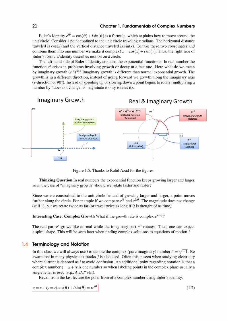
R Multiplication and Division amount to rotating complex numbers in one direction or anotherand scaling them. Most times it is useful to avoid the polar form and carry out these operationson the standard form. No matter which method is used the final answer should always bereported in standard form, x+ iy.
1.5.2 Complex Conjugation of an ExpressionDefinition 1.5.5 The conjugate of a sum of two complex numbers is the sum of the conjugates.Given z1 = x1 + iy1 and z2 = x2 + iy2, their sum
z1 + z2 =(x1 + x2)+ i(y1 + y2)= (x1+x2)−i(y1+y2)= (x1−iy1)+(x2−iy2)= z1+ z2. (1.11)
In addition, the conjugate of a difference, product, or quotient is equal to the difference, product,or quotient of the conjugates (e.g., z1− z2 = z1− z2, z1z2 = z1z2, and z1/z2 = z1/z2).
Example 1.14 i) (1+ i)(2−3i) = (1− i)(2+3i) = 2+3i−2i−3i2 = 2+ i+3 = 5+ iOR: 2−3i+2i−3i2 = 5− i = 5+ i.
ii) (1+ i)/(3−4i) = 1−i3+4i =
1−i3+4i
3−4i3−4i =
3−4i−3i+4i29+16 = −1−7i
25 =− 125 −
725 i
OR: 1+i3−4i
3+4i3+4i =
3+4i+3i+4i29+16 = −1+7i
25 = −125 + 7
25 i =− 125 −
725 i.
Notice z = f + ig where f ,g are complex numbers, then z = f + ig, NOT: f − ig.
Example 1.15 Let f = 1+ i or g = 2− i, then find z = f + ig.
Thus, z=(1+ i)+ i(2− i)= (1− i)− i(2+ i)= 2−3i. As a check find z=(1+ i)+ i(2− i)= 2+3i,then z = 2−3i 6= f − ig =−i.
Example 1.16 Show the conjugate of the quotient is the quotient of the conjugates.
Then z1z2= r1eiθ1
r2eiθ2= r1
r2ei(θ1−θ2) = r1
r2ei(θ2−θ1) = r1e−iθ1
r2eiθ1= z1
z2.
Observe that if it works for a sum then it automatically works for a difference A−B = A+(−B).If it works for a quotient, then it will work for a product A/B = A× (1/B).

30 Chapter 1. Fundamentals of Complex Numbers
1.5.3 Finding the Absolute Value |z|Definition 1.5.6 The magnitude or length of a complex number z is r = |z| =
√x2 + y2. We
take the positive square root since distance is positive.
Example 1.17 Given a complex number z = x+ iy find zz.
zz = (x+ iy)(x− iy) = x2− ixy+ ixy− i2y2 = x2 + y2 = r2 = |z|2 or in polar form zz = reiθ re−iθ =r2 = |z|2. Thus, |z|= r =
√zz.
Example 1.18 Find:
i) |1+ i|=√
12 +12 =√
2.
ii) |4i|=√
02 +42 =√
16 = 4.
iii) |1+2i|=√
12 +22 =√
5.
R The absolute value of a product or quotient is the product or quotient of the absolute values.
Example 1.19 i)∣∣1+i
1−i
∣∣= ∣∣1+i1−i
1+i1+i
∣∣= ∣∣∣1+i+i+i21+1
∣∣∣= ∣∣2i2
∣∣= |i|= 1
OR: |1+i||1−i| =
√12+12√
12+(−1)2=√
2√2= 1.
ii)∣∣2−3i
5+6i
∣∣= |2−3i||5+6i| =
√22+(−3)2√
52+62 =√
13√61
.
ii)∣∣2+4i
1+i
∣∣= |2+4i||1+i| =
√22+42√12+12 =
√20√2=√
10.
1.5.4 Complex EquationsThe main idea is to remember that a complex number is associated with a pair of real numbers (thereal and imaginary parts). Thus, a complex equation really contains two equations, one for the realparts and one for the imaginary parts.
Definition 1.5.7 Two complex numbers, z1 and z2, are equal if and only if x1 = x2 (real parts)and y1 = y2 (imaginary parts).
For example, 2+ i 6= 2− i. What does this say about complex equations? When solving acomplex equation we really need to solve two equations at once (for the real and imaginary parts).Knowing that an equations is complex gives a relationship between each part.
Example 1.20 Find z = x+ iy if z2 = 4i.
(x+ iy)2 = 4i
FOIL x2 +2ixy− y2 = 4i
Split into two equations Real: x2− y2 = 0, Imaginary: 2xy = 4.
Solving the first equation gives x2 = y2. Either x = −y or x = y. In the first case (x = −y), thesecond equation gives −2x2 = 4, which implies x =±=
√−2 =±2i, but we know x must be a
real number so this case cannot hold!
In the second case (x = y), the second equation gives 2x2 = 4 or x = ±√
2. Thus, the two so-lutions are (
√2,√
2) and (−√
2,−√
2).

1.5 Complex Algebra 31
Example 1.21 i) #39 Solve x+ iy = y+ ix.
Matching real and imaginary parts, this is always true if x = y. So there are infinitely manysolutions that lie on the line y = x in the complex plane.
ii) #44 Solve x+ iy = (1− i)2.
FOIL the left-hand side.
x+ iy = 1− i− i+ i2 = 1−2i−1 =−2i ⇒ x = 0, y =−2.
iii) #45 Solve (x+ iy)2 = (x− iy)2.
FOIL both sides.
x2 +2xyi− y2 = x2−2xyi− y2
2xyi =−2xyi
xy =−xy.
Thus, x =−x or y =−y. So either x = 0 or y = 0. Therefore, z = x or z = y.
Now for a harder example! If you can solve this you can handle most quadratic equations andhave demonstrated you follow all the necessary steps.
Example 1.22 x+iy+2+3ix+iy−3 = i+2. Let z = x+ iy and rewrite the equation as z+2+3i
z−3 = i+2.
z+2+3i = (i+2)(z−3)
z+2+3i = zi+−3i+2z−6
Rearrange terms with z: z− (2+ i)z =−3i−6− (2−3i)
(−1− i)z =−8−6i.
Thus, z = −8−6i−1−i = −8−6i
−1−i−1+i−1+i =
8−8i+6i−6i21+1 = 14−2i
2 = 7− i.
1.5.5 Graphs of Complex EquationsWhat is the curve made up of points in the complex plane satisfying |z|= 1?
In others words, find x and y such that x2 + y2 = 1. This is just the equation of a circle of ra-dius 1.
x
y

32 Chapter 1. Fundamentals of Complex Numbers
Example 1.23 Describe the plots of each of these complex equations:
i) |z− 3| = 4, square both sides |z− 3|2 = 16⇒ (x− 3)2 + y2 = 16. This is a circle centeredat (3,0) with radius 4.
ii) |z− 3| ≥ 4. This is the area outside the circle centered at (3,0) of radius 4 including thecircle boundary.
iii) |z−3|< 4. This is the interior of the circle centered at (3,0) of radius 4.
Recall the three basic conic sections and their equations
a) Circle centered at (a,b) of radius r (x−a)2 +(y−b)2 = r2
b) Ellipse centered at (a,b) with radius c in x and radius d in y(x−a)2
c2 +(y−b)2
d2 = 1
c) Hyperbola centers at (a,b)(x−a)2
c2 − (y−b)2
d2 = 1
Plot the solution to the equation θ = π/6
x
y
θ
Example 1.24 Plot each of the following:
i) Rez< 2
ii) Rez ≥ −1
iii) Imz ≥ 3.
1.5.6 Physical ApplicationsComplex Equations appear in all sorts of physical applications. Primarily adding analysis forproblems in two-dimensions. Classical examples are 2D fluid flow, superconductivity in a wire,among others. Understanding how complex equations work will provide the basis for learningadvanced methods. If interested further look up the techniques of conformal mapping or contourintegration, which are very useful in physics.
Example 1.25 A particle moves in the (x,y) plane so that its position as a function of time t is

1.6 Complex Infinite Series 33
given by
z = x+ iy =i+3tt−2i
.
Find the magnitudes of the velocity and the acceleration as a function of time.
Answer: First recall the definitions of position, velocity, and acceleration as well as their re-lationshipsPosition: z = x+ iyVelocity: dz
dt =dxdt + i dy
dt
Acceleration: d2zdt2 = d2x
dt2 + i d2ydt2
First find the velocity using the Quotient Rule, dzdt =
3(t−2i)−(i+3t)(t−2i)2)
= 3t−6i−i−3t(t−2i)2 = −7i
(t−2i)2 . We need to
find the magnitude so consider∣∣dz
dt
∣∣= |−7i||t2−4it−4| =
7√(t2−4)2+(4t)2
= 7√t4−8t2+16+16t2 =
7√t4+8t2+16
=
7√(t2+4)2
= 7t2+4 .
Now find the acceleration by taking one more derivative. d2zdt2 = 14i
(t−2i)3 . Last find its magnitude
a =
∣∣∣∣d2zdt2
∣∣∣∣=√
14i(t−2i)3
−14i(t +2i)3 =
14√(t3−6it2−12t +8i)(t3 +6it2−12t−8i)
,
then a = 14√(t2+4)3
= 14(t2+4)3/2 .
1.6 Complex Infinite Series
Recall that for a function of a real variable, f (x), we can find an approximation locally using aTaylor Expansion. Any function of one variable can be expanded about a point x = a as follows:
f (x+a) = f (a)+ f ′(a)(x−a)+f ′′(a)
2!(x−a)2 + ...+
f (k)(a)k!
(x−a)k + ...
Key Questions: Does this series converge? If so, then for what values of x is the expansion valid?We will explore these questions for complex Taylor Series.
Convergence in Section 2.6
Radius/Disk of Convergence in Section 2.7
For a real series we can define a partial sum of the first n terms, Sn := ∑nk=1 f (k)(a)(x−a)k. We
say the series converges if limn→∞ Sn = S where S is the sum.
R In future courses, you may see convergence defined different. Rigorously, a series is said toconverge if the partial sums get closer and closer together, |Sm−Sn| → 0 as m,n→ ∞.
Analogously, for complex numbers we say that the partial sum Sn = Xn + iYn consisting of asum in the real parts and a sum in the imaginary parts. The sum converges if both expressionsapproach some limit!
limn→∞
[Xn + iYn] = limn→∞
Xn + i limn→∞
Yn = X + iY.

34 Chapter 1. Fundamentals of Complex Numbers
Thus, Xn→ ∞ and Yn→ ∞. In other words, the real and imaginary parts of the series each convergeas a series of real numbers.
First, let’s review the definition of absolute convergence and convergence tests for series of realnumbers.
Definition 1.6.1 If the series of absolute values ∑∞n=1 |zn|<∞, then the series is called absolutely
convergence.
There is also a special type of series, which converges known as a geometric series.
Definition 1.6.2 A geometric series has the form: ∑∞i=1 ari. If |r| < 1 this series converges.
Useful formulas for the infinite sum and all partial sums are
n
∑i=1
ari = a(
1− rn
1− r
),
∞
∑i=1
ari =a
1− r.
1.6.1 Review from Calculus: Tests for ConvergenceFor more detail please consult Chapter 1 in the textbook by Boas.
Convergence TestIf the terms Xi 9 0, then the series must diverge.
Example 1.26 ∑∞i=1
ii+1 must diverge since each term Xi→ 1 6= 0.
Comparison TestConsider two series a1 +a2 +a3 + ... and b1 +b2 +b3 + .... If |an| ≤ |bn| for all n and the series∑bn converges, then the series for an is absolutely convergent OR if |an| ≥ dn and the series for dn
diverges, then the series for an diverges.
Example 1.27 ∑∞n=1
1n! = 1+ 1
2 +16 + .... Let bn =
12n , then |an| ≤ bn and ∑bn < ∞ (geometric
series). Thus an converges!
Integral TestIf 0 < an+1 ≤ an for n > N, then ∑
∞n=1 an converges/diverges if
∫∞
0 andn converges/diverges.
Example 1.28 ∑∞n=1
1n . Using the Integral Test:
∫∞
11n dn = ln(n)
∣∣∣∣∞1= ln(∞)− 0→ ∞. So the
original series diverges!
Ratio TestTake the ratio of two consecutive terms in the series: ρn =
∣∣∣an+1an
∣∣∣ and consider limn→∞ ρn. If:i) ρ < 1 the series convergesii) ρ > 1 the series divergesiii) ρ = 1 there is not enough info to conclude if the series converges or diverges.
Example 1.29 ∑∞n=1
1n! , then ρn =
∣∣∣ 1(n+1)!
n!1
∣∣∣ = n!(n+1)! =
1n+1 → 0. Thus, the original series
converges.
Root TestConsider the nth root of the summand L := limn→∞
n√|an|. If:
i) L < 1 the series is absolutely convergentii) L > 1 the series is divergentiii) L = 1 there is not enough info to conclude if the series converges or diverges.
Example 1.30 ∑∞n=0
(5n−3n3
7n3+2
)n, then L =
∣∣∣5n−3n3
7n3+2
∣∣∣= ∣∣−37
∣∣= 37 < 1. The series converges!

1.7 Complex Power Series and Disk of Convergence 35
Alternating SeriesAn alternating series is a series where the terms have the form an = (−1)nbn or an = (−1)n+1bn.An alternating series converges if the limit of the absolute value of the terms converges to zero andthe terms are decreasing: |an+1|< |an| and limn→∞ an = 0.
Example 1.31 1− 12 +
13 −
14 +
15 −
16 + ..., converges by the alternating series test.
Definition 1.6.3 If a series converges, but not absolutely, then it is said to be conditionallyconvergent. This is a weaker form of convergence. In particular, the terms in the sum can berearranged to form any total. In contrast, for a series that is absolutely convergent, rearrangingthe terms does not change the sum.
1.6.2 Examples with Complex Series
Example 1.32 i) 1+ (i+2)3 + (i+2)2
9 + (i+2)3
27 + ...+ (2+i)n
3n + ....
By the Ratio Test: limn→∞ |ρn| = limn→∞
∣∣∣ (2+i)n+1
3n+13n
(2+i)n
∣∣∣ = ∣∣2+i3
∣∣ = √22+12
3 =√
53 < 1. The se-
ries converges!
ii) ∑∞n=1
in√n .
Consider the Real Part: ∑∞n=1
(−1)n√
2nand Imaginary Part: ∑
∞n=0
(−1)n√
2n+1. Both series converge by
the alternating series test. Thus, the complex series converges!
iii) ∑∞n=0(z+1)n.
Using the Root Test: L := limn→∞ |z + 1| converges for |z + 1| < 1 or√
(x+1)2 + y2 < 1 or(x+1)2 + y2 < 1. Thus, the series converges for z inside the circle centered at (−1,0) of radius 1not including the boundary.
1.7 Complex Power Series and Disk of ConvergenceRecall from calculus a power series for a function of a real variable (centered at zero)
f (x) =∞
∑n=1
anxn =∞
∑n=1
f (n)(0)n!
xn,
or centered at point x = a
f (x) =∞
∑n=1
bn(x−a)n =∞
∑n=1
f (n)(a)n!
(x−a)n.
Definition 1.7.1 (Interval of Convergence) The values of x where the series converges.
Example 1.33 Given the power series ∑xn. By the ratio test ρ :=∣∣∣ xn+1
xn
∣∣∣= |x|. For convergencewe need ρ < 1. Thus, |x|< 1 is the interval of convergence.
Before defining a complex power series, let’s discuss some facts for real power series (reviewfrom Calculus):
1. A power series can be differentiated or integrated term by term. The resulting series con-verges to the derivative or integral of the original function within the same interval of convergence.

36 Chapter 1. Fundamentals of Complex Numbers
Example 1.34 Consider the function f (x) = ex, which has power series ∑∞n=0
xn
n! .
a) Differentiating term by term: ∑∞n=1
nxn−1
n! = ∑∞n=1
xn−1
(n−1)! →k:=n−1 ∑∞k=0
xk
k! = ex.
b) Integrating term by term: ∑∞n=0
xn+1
(n+1)! →k:=n+1 ∑∞k=1
xk
k! = ex−1. Note∫
ex = ex +C.
c) The Interval of Convergence (I.O.C.) can be found using the ratio test ρ :=∣∣∣∣ xn+1
(n+1)!xnn!
∣∣∣∣= limn→∞
∣∣ xn+1
∣∣→0. Thus, the interval of convergence is all real numbers.
2. Two power series can be added, subtracted, multiplied. The result converges in the commoninterval of convergence.
3. One series can be substituted into another if the substituted series values are in the inter-val of convergence of the series it is being plugged into.
4. The power series of a function is unique! Only one power series of the form ∑n anxn con-verges to a given function.
R Properties 1.-4. still hold for complex power series!
Definition 1.7.2 A complex power series has the form ∑n anzn where z = x+ iy. The realpower series just a special case of the complex power series when y = 0.
Example 1.35 i) 1+ z+ z2
2 + z3
6 + ...= ∑∞n=0
zn
n!
ii) 1− i(z+1)+ (i[z+1])2
2 + (i[z+1])3
6 + (i[z+1])4
24
iii) ∑∞n=0
(z−2+2i)n
6nn3 .
Definition 1.7.3 The complex analogue of the radius of convergence is the disk of convergence(in the 2D complex plane).
Example 1.36 Find the Disk of Convergence (D.O.C.) for each complex power series in theprevious example.
i) For ∑∞n=1
zn
n! , use the ratio test. ρ := limn→∞
∣∣∣ zn+1
(n+1)!n!zn
∣∣∣ = limn→∞
∣∣ zn+1
∣∣→ 0. Thus, the seriesconverges for all z in the complex plane. Therefore, the disk of convergence is the entire complexplane, C.
ii) For 1+∑∞n=1
(i[z+1])n(−1)n
n . By the ratio test ρ = limn→∞
∣∣∣ (i[z+1])n+1(−1)n+1
n+1n
(i[z+1])n(−1)n
∣∣∣= limn→∞
∣∣∣ i(z+1)(−1)nn+1
∣∣∣→|z+1|
1 . Thus, ρ < 1 if |z+1|< 1. Thus, the disk of convergence is the interior of the circle centeredat (−1,0) with radius 1.

1.8 Elementary Functions of Complex Numbers 37
x
y
(−1,0)(−2,0) ••
iii) ∑∞n=0
(z−2+2i)n
6nn3 . Use the ratio test, ρ = limn→∞
∣∣∣ (z−2+2i)n+1
6n+1(n+1)36nn3
(z−2+2i)n
∣∣∣= limn→∞
∣∣∣ (z−2+2i)n3
6(n+1)3
∣∣∣→∣∣ z−2+2i6
∣∣. Thus, the series converges if ρ < 1 or |z−2+2i|< 6. The disk of convergence is centeredat (2,−2) of radius
√6.
Example 1.37 iv) 1− z2
3! +z4
5! + .... General Form: ∑∞n=0
(−1)nz2n
(2n+1)! . Then by the ratio test,
ρ = limn→∞
∣∣∣ (−1)n+1z2(n+1)
[2(n+1)+1]!(2n+1)!(−1)nz2n
∣∣∣ = limn→∞
∣∣∣ (−1)z2
(2n+3)(2n+2)
∣∣∣→ 0. Thus, the disk of convergenceis the entire complex plane, C.
v) ∑∞n=0 2n+1(z+ i−3)2(n+1). Then by the ratio test, ρ = limn→∞
∣∣∣2n+1(z+i−3)2(n+1)
2n(z+i−3)2n
∣∣∣= limn→∞ |2(z+i−3)2|= |2(z+ i−3)2|. the disk of convergence is where |(z+ i−3)|2 < 1
2 or the disk centered at(3,−1) of radius 1/
√2.
1.8 Elementary Functions of Complex NumbersIn principle we can consider any function we have traditionally used (e.g., exponential, trig functions,polynomials). In the previous section we saw complex polynomials in the form of power series.We start this section with the next level of complexity, rational functions (ratios of polynomials):
f (z) =a0 +a1z+a2z2 + ...+aNzN
b0 +b1z+b2z2 + ...+bMzM .
Example 1.38 Given the complex function f (z) = z3−1z+2 , find f (i−1).
Step 1: Substitute value of z into the function
f (i−1) =(i−1)3−1(i−1)−2
.
Step 2: Simplifying
f (i−1) =(i−1)(i2−2i+1)−1
i+1=
(i−1)(−2i)−1i+1
=−2i2 +2i−1
i+1=
1+2ii+1
Step 3: Rationalize the denominator (Multiply by the complex conjugate over itself)
f (i−1) =1+2ii+1
1− i1− i
=1+2i− i−2i2
2=
32+
12
i
More Examples in Class!

38 Chapter 1. Fundamentals of Complex Numbers
Recall the power series for ex = ∑∞n=0
xn
n! in real numbers. Can we make a similar definition forthe complex exponential function?
Definition 1.8.1 Using the definition of the power series expansion of the exponential functionof real variables, replace x with z:
ez =∞
∑n=0
zn
n!(1.12)
Where does it converge (Disk of Convergence)?
By the Ratio Test: ρ = limn→∞
∣∣∣ zn+1
(n+1)!n!zn
∣∣∣ = limn→∞
∣∣ zn+1
∣∣ → 0. Thus, ρ > 1 for all z in theComplex Plane and the disk of convergence must be C.
Operations with Complex Exponential Functions
Example 1.39 i) ez1ez2 =[(1+ z1 +
z212 + ...)(1+ z2 +
z222 + ...)
]=[1+(z1 + z2)+
(z1+z2)2
2
]=
ez1+z2
ii) Note: ddz [z
n] = nzn (just like normal derivatives of real numbers!
ddz [e
z] = ddz
(1+ z+ z2
2 + ...+ zn
n! + ...)= 0+1+ z+ z2
2 + ...+ nzn−1
n! + ...
= 0+1+ z+ z2
2 + ...+ zn−1
(n−1)! + ...= ez
1.9 Euler’s FormulaRecall the Taylor expansion for the basic trig functions of one real variable
sin(x) = x− x3
3!+
x5
5!− x7
7!+ ...
cos(x) = 1− x2
2!+
x4
4!− x6
6!+ ...
Can we do something similar for complex trig functions? First, consider the complex Taylor seriesfor the exponential function
eiθ = 1+ iθ +(iθ)2
2!+
(iθ)3
3!+
(iθ)4
4!+
(iθ)5
5!+ ...
= 1+ iθ − θ 2
2!− i
θ 3
3!+
θ 4
4!+ i
θ 5
5!+ ...
=
[1− θ 2
2!+
θ 4
4!+ ...
]+ i[
θ − θ 3
3!+
θ 5
5!+ ...
]= cos(θ)+ isin(θ).
This result gives us Euler’s Formula!
eiθ = cos(θ)+ isin(θ) (1.13)
We have been using this formula since Section 3.2, but now we can see why it holds. We also haveverified
z = x+ iy = r(cos(θ)+ isin(θ) = reiθ . (1.14)

1.9 Euler’s Formula 39
Example 1.40 Find the values of 3eiπ/3,eiπ/2,2e−iπ/6,e2nπi.
i) 3eiπ/3⇒ r = 3,θ = π/3. Recall from polar coordinates x= r cos(θ) = 3cos(π/3) = 3(1
2
)= 3/2
and y = r sin(θ) = 3sin(π/3) = 3(√
32
)= 3
√3
2 . Thus, z = 32 +
3√
32 i.
ii) eiπ/2 ⇒ r = 1,θ = π/2. Recall from polar coordinates x = r cos(θ) = cos(π/2) = 0 andy = r sin(θ) = sin(π/2) = 1. Thus, z = i.
iii) 2e−iπ/6 ⇒ r = 2,θ = −π/6. Recall from polar coordinates x = r cos(θ) = 2cos(−π/6) =2cos(π/6) = 2
(√3
2
)=√
3 and y = r sin(θ) = 2sin(−π/6) =−2sin(π/6) = 2(−1
2
)=−1. Thus,
z =√
3− i.
iv) e2nπi⇒ r = 1,θ = 2nπ . Recall from polar coordinates x = r cos(θ) = 1 and y = r sin(θ) = 0.Thus, z = 1 for all n.
Recall that Euler’s Formula/Identity is especially useful for multiplying and dividing complexnumbers
z1z2 = r1eiθ1r2eiθ2 = r1r2ei(θ1+θ2)
z1/z2 =r1eiθ1
r2eiθ2=
r1
r2ei(θ1−θ2)
Example 1.41 Evaluate (1−i)2
1+i .
Step 1: Write in Polar Form: z1 = (1− i)2 =[√
2e−iπ/4]2
= 2e−iπ/2 and z2 = 1+ i =√
2eiπ/4.
Step 2: Carry out the multiplication or division:
z1
z2=
2e−iπ/2√
2eiπ/4=
2√2
ei(−π/2−π/4) =√
2ei3π/4.
Step 3: Write in Standard Form, z = x+ iy. z =√
2ei3π/4 =−1− i.
Example 1.42 Evaluate (2+2√
3i)(1+ i).
Step 1: Write in Polar Form: z1 = (2+2√
3i) = 4eiπ/3 and z2 = 1+ i =√
2eiπ/4.
Step 2: Carry out the multiplication or division:
z1z2 = 4√
2ei(π/3+π/4) = 4√
2ei7π/12.
Step 3: Write in Standard Form, z = x+ iy, if an easy angle (e.g., 30-60-90, 45-45-90). Here 7π/12is not an angle that can be handled easily by hand, so we will leave it in polar form.
Example 1.43 Evaluate (1+ i)(1− i).
Step 1: Write in Polar Form: z1 = 1+ i =√
2eiπ/4 and z2 = 1− i =√
2e−iπ/4.
Step 2: Carry out the multiplication or division:
z1z2 = 2ei(π/4−π/4) = 2ei0 = 2
Step 3: Write in Standard Form, z = x+ iy, if an easy angle (e.g., 30-60-90, 45-45-90). Notice(1+ i)(1− i) = 1+ i− i− i2 = 2.
40 Chapter 1. Fundamentals of Complex Numbers
1.10 Powers and Roots of Complex Numbers
We have clear definitions for powers and roots (fractional powers) of real numbers. Can we definethe analogous notions for complex numbers?
Given a complex number z, consider it raised to the nth power.
Definition 1.10.1 To raise a complex number to the nth power one needs to raise the modulus,r, to the nth power and multiply the angle by n.
zn =[reiθ]n
= rneinθ (1.15)
Another useful idea using this definition is Demoivre’s Theorem:
Theorem 1.10.1 (Demoivre’s Theorem) When r = 1, the nth power can be expressed int hefollowing way:(
eiθ)n
= (cos(θ)+ isin(θ))n = cos(nθ)+ isin)nθ). (1.16)
Example 1.44 Evaluate (1+ i)4.
Step 1: Write in Polar Form: 1+ i =√
2eiπ/4
Step 2: Carry out the calculation using the definition.
(1+ i)4 =[√
2eiπ/4]4
= (√
2)4eiπ = 4 [cos(π)+ isin(π)] = 4[−1+0] =−4. (1.17)
Now we want to consider taking the nth root. Recall that taking the nth root of a real numberis equivalent to raising that number to the 1
n power. Similarly, for a complex number, n√
z = z1/n.
Definition 1.10.2 To take the nth root of a complex number one needs to take the nth root ofthe modulus, r, and divide the angle by n.
n√
z = z1/n =[reiθ]1/n
= r1/neiθ/n = n√
r [cos(θ/n)+ isin(θ/n)] . (1.18)
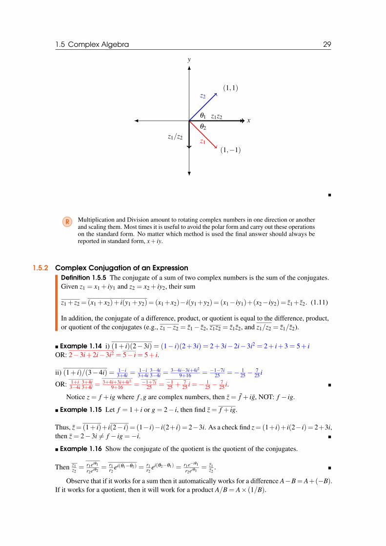
Example 1.45 Find the cube roots of 64. In other words, find z so that z3 = 64. Let’s at-tack this problem using the polar form of the complex number, z = 64. Thus, r = 64 andθ = 0,2π,4π, ...,2πn. Now, by the definition of the root: z1/3 = r1/3eiθ/3 = r1/3ei(2πn+θ)/3 ⇒r = 4,θ = 0,2π/3,4π/3,6π/3, .... Observe that 6π/3 = 2π = 0 (on the complex plane). Thus, thethree roots are: 4ei0 = 4,4ei2π/3,4e4π/3 or z = 4,−2+2
√3i,−2−2
√3i.
As a check: (−2+ 2√
3i)3 = (−2+ 2√
3i)(4− 8√
3i− 12) = (−2+ 2√
3i)(−8− 8√
3i) = (16+16√
3i−16√
3i+48) = 64.

1.10 Powers and Roots of Complex Numbers 41
x
y
(4,0)
(−2,2√
3)
(−2,−2√
3)
•
•
•
R Always remember that complex numbers always come in conjugate pairs!
Example 1.46 Find the 4th roots of -81. In other words, find z so that z4 =−81. Use the polarform of the complex number, z =−81. Thus, r = 81 and θ = π,3π,5π,7π, ...,π +2πn.
Now, by the definition of the root: z1/4 = r1/4eiθ/4 = r1/4ei(2πn+θ)/4⇒ r = 3,θ = π/4,3π/4,5π/4,7π/4, ....Observe that 9π/4 = π/4 (on the complex plane).
Thus, the four roots are: 3eiπ/4,3ei3π/4,3ei5π/4,3ei7π/4 or z = 3√
22 + i 3
√2
2 , 3√
22 − i 3
√2
2 ,−3√
22 +
i 3√
22 ,−3
√2
2 − i 3√
22 .
As a check: (3√
22 + i 3
√2
2 )4 = (184 + 36
4 i− 184 )(
184 + 36
4 i− 184 ) = (9i)(9i) =−81.
x
y
(3√
2/2,3√
2/2)
(3√
2/2,−3√
2/2)
(−3√
2/2,3√
2/2)
(−3√
2/2,−3√
2/2)
•
•
•
•

42 Chapter 1. Fundamentals of Complex Numbers
Example 1.47 Find and plot the values of 6√−64.
Thus, we need to find r,θ such that(reiθ)6
= −64. Consider the polar form of −64, wherer = 64 and θ = π,3π,5π,7π,9π,11π .
Now, by the definition of the root: z1/6 = r1/6eiθ/6 = r1/6ei(2πn+θ)/6⇒ r = 2,θ = π/6,π/2,5π/6,7π/6,3π/2,11π/6, ....Observe that 13π/6 = π/6 (on the complex plane).
Thus, the six roots are: 2eiπ/6,2eiπ/2,2ei5π/6,2ei7π/6,2ei3π/2,2ei11π/6 or z =√
3+ i,2i,−√
3+i,−√
3− i,−2i,√
3− i.
x
y
(√
3,1)
(0,2)
(−√
3,1)
(−√
3,−1)
(0,−2)
(√
3,−1)
•
•
•
•
•
•
1.11 The Exponential and Trigonometric Functions
Recall from a previous section the power series expansion for ez = 1+ z+ z2
2! + ... zn
n! + .... This canbe written in another form:
ez = ex+iy = exeiy = ex [cos(y)+ isin(y)] .
This new form using Euler’s Formula may be easier to use in some instances.
Example 1.48 i) e3+iπ/2 = e3eiπ/2 = e3 [cos(π/2)+ isin(π/2)] = e3 [0+ i] = e3i.
ii) e3ln3−iπ/2 = eln(27)e−iπ/2 = 27 [cos(−π/2)+ isin(−π/2)] = 27[0− i] =−27i.
Recall Euler’s Formula:
eiθ = cos(θ)+ isin(θ) (1.19)
e−iθ = cos(θ)− isin(θ) (1.20)

1.11 The Exponential and Trigonometric Functions 43
Subtracting (8.114) from (8.54):
eiθ − e−iθ = 2isin(θ) ⇒ sin(θ) =eiθ − e−iθ
2i.
Adding (8.54) to (8.114) gives:
eiθ + e−iθ = 2cos(θ) ⇒ cos(θ) =eiθ + e−iθ
2.
These expressions hold for real θ , but can be extended to all complex numbers, z, by replacingθ 7→ z.
Definition 1.11.1 (Complex Trigonometric Functions)
sin(z) =eiz− e−iz
2cos(z) =
eiz + e−iz
2. (1.21)
The remaining trigonometric functions can be derived using the usual relations:
tan(z) =sin(z)cos(z)
, cot(z) =cos(z)sin(z)
, csc(z) =1
sin(z), sec(z) =
1cos(z)
. (1.22)
Example 1.49 Find sin(i).
Using the definition:
sin(i) =ei2− e−i2
2i=
e−1− e1
2i≈ 1.1752i.
R One interesting difference from real numbers is the range for sine and cos. For real x,|sin(z),cos(z)| ≤ 1. This bound does not hold for the complex forms of sine and cosine asseen by the previous example.
We can recover some of the same calculus trig identities for the complex versions.
Example 1.50 Does sin2(z)+ cos2(z) = 1?
Check: sin2(z) =(
eiz−e−iz
2i
)2= e2iz−2+e−2iz
−4 .
Check: cos2(z) =(
eiz+e−iz
2i
)2= e2iz+2+e−2iz
4 .
So, sin2(z)+ cos2(z) = 44 = 1.
Example 1.51 Show the double angle formula: sin(2z) = 2cos(z)sin(z).
sin(2z) = e2iz−e−2iz
2i = (eiz+e−iz)(eiz−e−iz)2i = 2
[eiz+e−iz
2
][eiz−e−iz
2i
]= 2cos(z)sin(z).
What about the derivatives of the sine and cosine? Are they the same or very different?
Example 1.52 i) ddz sin(z) = d
dz
[eiz−e−iz
2i
]= ieiz+ie−iz
2i = eiz+e−iz
2 = cos(z). Same!
ii) ddz cos(z) = d
dz
[eiz+e−iz
2
]= ieiz−ie−iz
2 =−[
eiz−e−iz
2i
]=−sin(z). Same!

44 Chapter 1. Fundamentals of Complex Numbers
1.12 Hyperbolic FunctionsWhat do sine and cosine look like when a complex number is purely imaginary, z = iy?
sin(iy) =ei(iy)− e−i(iy)
2i=
e−y− ey
2i= i
ey− e−y
2
cos(iy) =ei(iy)+ e−i(iy)
2=
e−y + ey
2=
ey + e−y
2.
These are special functions and come up when solving dynamic problems (differential equations,more in Math Methods II!).
Definition 1.12.1 (Hyperbolic Trig Functions)
sinh(z) =ez− e−z
2cosh(z) =
ez + e−z
2. (1.23)
Similarly,
tanh(z) =sinh(z)cosh(z)
, coth(z) =cosh(z)sinh(z)
, sech(z) =1
cosh(z), csch(z) =
1sinh(z)
. (1.24)
Thus, observe that sin(iy) = isinh(y) and cos(iy) = cosh(y). Now consider some trig identitieswith hyperbolic trig functions.
Example 1.53 Show: cosh2(z)− sinh2(z) = 1
Using the definition, cosh2(z) =[
ez+e−z
2
]2= e2z+2+e−2z
4
Also, using the definition: sinh2(z) =[
ez−e−z
2
]2= e2z−2+e−2z
4 . So, cosh2(z)− sinh2(z) = 44 = 1.
We also can consider the derivatives of the hyperbolic trig functions:
Example 1.54 i) ddz sinh(z) = d
dz
[ez−e−z
2
]= ez+e−z
2 = cosh(z).
ii) ddz cosh(z) = d
dz
[ez+e−z
2
]= ez−e−z
2 = sinh(z).
R Observe that there is no sign change when taking the derivative of the hyperbolic cosine. Thisis in contrast to normal trig functions where d
dz cos(z) =−sin(z).
Exercise 1.1 Why are complex roots of quadratic equations always found in pairs?
Hint: Look at the Quadratic Formula, which is valid for any quadratic equation.

II
2 Fundamentals of Linear Algebra . . . . . . 472.1 Systems of Linear Equations2.2 Row Reduction and Echelon Forms2.3 Determinants and Cramer’s Rule2.4 Vectors2.5 Lines, Planes, and Geometric Applications2.6 Matrix Operations2.7 Linear Combinations, Functions, and Operators2.8 Matrix Operations and Linear Transformations2.9 Linear Dependence and Independence2.10 Special Matrices2.11 Eigenvalues and Eigenvectors2.12 Diagonalization
Part Two: Linear Algebra


2. Fundamentals of Linear Algebra
Linear Algebra basically refers to linear relationships between objects. Can we think of examplesof linear functions we have seen in the past?
Definition 2.0.2 A function f (x) is linear if:
1. f (x+ y) = f (x)+ f (y).
2. f (cx) = c f (x) for any real number c.
Linear algebra takes this idea to the next level of abstraction by introducing the idea of a linearoperation. The idea is to take a system of linear equations and solve them simultaneously usingobject called matrices. This section will start by introducing the relationship between matrices andsystems of linear equations. After the basic definitions are known we will begin to explore how towork with these objects to solve real problems.
2.1 Systems of Linear EquationsFirst we must define what is meant by a single Linear Equation.
Definition 2.1.1 (Linear Equation) A linear equation is any equation of the form
a1x1 +a2x2 + ...+anxn = b,
where a1, ...,an,b are constant real numbers and x1, ...,xn are the unknown variables.
Example 2.1 Are the following equations linear?
i) 4x1−5x2 +2 = x1
If we rearrange we find: 3x1−5x2 =−2, so yes!

48 Chapter 2. Fundamentals of Linear Algebra
ii) x2 = 2(√
6− x1)+ x3
If we rearrange we find: 2x1 + x2− x3 = 2√
6, so yes!
Sometime it is easier to see if an equation meets any of these easy cases for being nonlinear torule out linearity:
i) Products of Variables: x1x2 + x3 = 4 is Nonlinear
ii) Trig. Functions: sin(x1)+ x2 = 2 is Nonlinear
iii) Powers/Roots: x2,x1/2 are Nonlinear.
Definition 2.1.2 (A System of Linear Equations) A system of linear equations is a collection ofone or more linear equations involving the same set of variables (e.g., x1, ...,xn).
Definition 2.1.3 (Solution of a Linear System) A list (s1,s2, ...,sn) of numbers that makeseach equation in the system true when the values s1,s2, ...,sn are substituted for x1,x2, ...,xn
respectively.
Example 2.2 Possible solutions for two equations in two variables:
i) One Unique Solution (Consistent):
x1 + x2 = 10
−x1 + x2 = 0
ii) No Solution (Inconsistent):
x1−2x2 =−3
2x1−4x2 = 8
iii) Infinitely Many Solutions (Consistent):
x1 + x2 = 3
−2x1−2x2 =−6
Definition 2.1.4 (Equivalent Systems) Two linear systems with the same solution set.
2.1.1 Matrix NotationGiven a linear system in Standard Form:
x1−2x2 =−1
−x1 +3x2 = 3
we can define two associated matrices. The first is the coefficient matrix made up of the coefficientsof each variable:[
1 −2−1 3
],
and the augmented matrix that is composed of the coefficients and the righthand side[1 −2 −1−1 3 3
].

2.2 Row Reduction and Echelon Forms 49
2.1.2 Elementary Row OperationsThere are three basic operations we can perform on an augmented matrix without changing itssolution set:1. (Replacement) Add one row to a multiple of another row.2. (Interchange) Switch two rows.3. (Scaling) Multiply all entries in a row by a nonzero constant.
These three operations are your only valid tools in attacking problems involving matrices. Wewill learn more advanced methods throughout the course, but for now we will stick with these threerules.
Definition 2.1.5 (Row Equivalent Matrices) Two matrices where one matrix can be transformedinto the other matrix by a sequence of elementary row operations.
Fact: If the augmented matrices of two linear systems are row equivalent, then thetwo systems have the same solution set.
Definition 2.1.6 (Size of a Matrix) We say a matrix with m rows and n columns is an m× nmatrix. Thus, a 2×3 matrix has two rows and three columns. In fact the Matrix A is composedof elements (numbers) ai j where i corresponds to the row and j the column.
Example 2.3 Use the three elementary row operations to solve the following linear system:
x1−2x2 + x3 = 0
2x2−8x3 = 8
−4x1 +5x2 +9x3 =−9,
Step 1: Put the equations into Standard FormStep 2: Find the augmented matrix for the system of linear equationsStep 3: Row reduce using elementary row operationsStep 4: Back Substitute the values into the system to solve.
Solution: (29,16,3)
Final Step: Check by plugging the solution back into the original system.
2.1.3 Fundamental Questions In Linear Algebra1. Is the system consistent? (Does a solution exist?)
2. If a solution exists, is it unique? (Is there one and only one solution)?These questions are answered during the course of elementary row operations.
If the augmented matrix ever has a row with all zeros except the last element is nonzero, [00...0b],then the system is inconsistent and there is no solution!
More on uniqueness in the next section (hint: it will have to do with the concept of pivot variables).
2.2 Row Reduction and Echelon Forms

50 Chapter 2. Fundamentals of Linear Algebra
Definition 2.2.1 (Echelon Form). A matrix is in echelon form if:
1. All nonzero rows are above any rows of all zeros.2. Each leading entry (e.g., left most entry, also called pivot) of a row is in a column to the rightof the leading entry of the row above it.3. All entries in a column below a leading entry are zero.
Definition 2.2.2 (Reduced Echelon Form). A matrix is in reduced echelon form if in addition to1.-3.:
4. The leading entry in each nonzero row is 1.5. Each leading 1 is the only nonzero entry in its column.
Example 2.4 i) Row reduce the following matrix to echelon form and locate the pivot columns(columns which contain a pivot).
0 −3 −6 4 9−1 −2 −1 3 1−2 −3 0 3 −11 4 5 −9 −7
Row reduce to see that the pivot columns are 1, 2, and 4. There can be no more than 1 pivot in anyrow.
ii) Row reduce the following matrix to reduced echelon form. 0 −3 −6 6 4 −53 −7 8 −5 8 93 −9 12 −9 6 12
2.2.1 Solutions of Linear SystemsDefinition 2.2.3 A basic variable is any variable that corresponds to a pivot column in theaugmented matrix of a system.
A free variable is any variable that is not a basic variable.
The final step in solving any linear system is writing all the basic variables in terms of any freevariables.
Example 2.5
1 6 0 3 0 00 0 1 −8 50 0 0 0 1 7
⇒
x1 =−6x2−3x4
x2 is freex3 = 5+8x4
x4 is freex5 = 7.
2.3 Determinants and Cramer’s Rule 51
Definition 2.2.4 The general solution of a system of linear equations provides a parametricdescription of the solution set.
Thinking Question: The above example has infinitely many solutions. Why is it true?
Definition 2.2.5 The Transpose of a matrix denoted AT is the matrix formed when the rowsand columns of A are switched. (AT )i j = A ji, and thus the transpose of an m×n matrix is ann×m matrix.
Example 2.6 Given a matrix A =
[1 2 34 5 6
], find its transpose.
AT =
1 42 53 6
.
Definition 2.2.6 (Rank of a Matrix) The number of nonzero rows remaining when a matrix hasbeen row reduced is the rank of the matrix.
If we know the rank of a matrix we know how many solutions to expect based on the originalsize of the matrix, M is m×n and A is the row-reduced augmented matrix. Consider the generalproblem of solving m equations in n unknowns:1. If rank(M)< rank(A), the equations are inconsistent .2. If rank(M) = rank(A) = n (the number of unknowns), there is exactly one solution.3. If rank(M) = rank(A) = R < n, then there are R basic variables and n−R free variables resultingin infinitely many solutions.
2.3 Determinants and Cramer’s Rule
Recall in the last lecture we introduced the concept of a matrix to provide a convenient andorganized way to solve a system of linear equations. The main concepts from the last section werethe elementary row operations and deciding whether a matrix has none, one or infinitely manysolutions. An arbitrary m×n matrix is just a display of coefficients for m equations in n unknowns.Through this next section we focus on a special type of matrix called a square matrix. In this casethe matrix has the exact same number of rows and columns (e.g., n×n).
Now that we have these matrices we want to use them to do more advanced things then simplysolving linear systems. The first basic quantity associated to any square matrix that will be usefulgoing forward is the determinant. The determinant can be though of as a measure of volume insome sense (more to come on this later). The loose analog for real numbers is the absolute value,| · |.
Start with the simplest case of a 2×2 matrix of the form
A =
[a bc d
]. (2.1)
Definition 2.3.1 The determinant of a 2×2 matrix A, denoted |A|, is defined to be
|A|=∣∣∣∣ a b
c d
∣∣∣∣= ad−bc. (2.2)
Note that the determinant of a 1×1 matrix, A = a is a trivial extension of this idea |A|= a.

52 Chapter 2. Fundamentals of Linear Algebra
Example 2.7 i) Find the determinant of A =
[1 23 4
].
det(A) =∣∣∣∣ 1 2
3 4
∣∣∣∣= 1(4)−2(3) = 4−6 =−2.
ii) Find the determinant of A =
[1 22 4
].
det(A) =∣∣∣∣ 1 2
2 4
∣∣∣∣= 1(4)−2(2) = 4−4 = 0.
In order to introduce a formula for the determinant of an arbitrary n×n matrix we first mustintroduce some notation. Given a matrix A we can define a sub-matrix Ai j where the ith row andjth column have been deleted.
Example 2.8
A =
1 2 3 45 6 7 89 10 11 1213 14 15 16
, A23 =
1 2 49 10 1213 14 16
.
Definition 2.3.2 (Determinant of an n× n Matrix) For n ≥ 2, the determinant of an n× nmatrix A is given by
det(A) = a11det(A11)−a12det(A12)+ ...+(−1)1+na1ndet(A1n) =n
∑j=1
(−1)1+ ja1 jdet(A1 j).
(2.3)
This process is call Cofactor Expansion.
Thus, for an n×n matrix we keep applying cofactor expansion until all the remaining determi-nants are 2×2.
Example 2.9 i) Compute the determinant of A =
1 2 03 −1 22 0 1
Solution: 1
ii) Compute the determinant of A =
1 0 00 2 00 0 3
Solution: 6
R Cofactor expansion can actually be done about any row or column not just the first one
|A|= det(A) =
∑
nj=1(−1)i+ jai jdet(Ai j) Expand about row i
∑ni=1(−1)i+ jai jdet(Ai j) Expand about column j.
(2.4)
Example 2.10 i) Compute the determinant of A =
1 2 03 −1 22 0 1
using cofactor expansion
about the third column

2.3 Determinants and Cramer’s Rule 53
Solution: 1
ii) Compute the determinant of A =
1 2 3 40 2 1 50 0 2 10 0 3 5
Solution: 14
2.3.1 Special Case: Upper and Lower Triangular Matrices
Definition 2.3.3 An n×n matrix A is said to be upper triangular if all the elements below themain diagonal, ai j for i < j, are zero. An n×n matrix A is said to be lower triangular if all theelements above the main diagonal, ai j for i > j, are zero. Finally, a matrix is said to be diagonalif the only nonzero elements are in positions (i, i) for i = 1, ...,n.
FACT: If a matrix A is one of the three cases of triangular matrices (e.g., upper, lower, diagonal),then the determinant is just the product of the diagonal elements.
Example 2.11 i) Compute the determinant of A =
1 2 00 −1 20 0 1
Solution: -1
ii) Compute the determinant of A =
2 3 4 50 1 2 30 0 −3 50 0 0 4
Solution: -24
2.3.2 Properties of Determinants
Facts:1. If each element of one row or one column of a determinant is multiplied by a number k, the valueof the determinant is multiplied by k.
2. The value of a determinant is zero if one of the following occurs:(a) All elements of one row or column are zero.(b) Two rows or two columns are identical.(c) Two rows or two columns are proportional.
3. If two rows or two columns of a determinant are interchanged, the value of the determi-nant changes sign.
4. The value of a determinant is unchanged if:(a) Row are written as columns and columns as rows (e.g., det(A) = det(AT )).(b) We add to each element of one row, k times the corresponding element of another row, where kis any number (and a similar statement for columns).

54 Chapter 2. Fundamentals of Linear Algebra
Example 2.12 i) Find the determinant of A =
1 2 3 40 5 0 02 7 6 102 9 7 11
.
Solution: -10.
ii) Find the determinant of A =
2 4 65 6 77 6 10
.
Solution: -40.
iii) Find the determinant of A =
2 3 0 14 7 0 37 9 −2 41 2 0 4
.
Solution: -12.
Example 2.13 (Application) Find the equation of a plane through (0,0,0),(1,0,1),(1,2,0).Recall the equation of a plane has the form ax+by+ cz+d = 0. Treat a,b,c,d as the unknowns.We can setup the following determinant problems to find the equation of the plane
∣∣∣∣∣∣∣∣x y z 10 0 0 11 0 1 11 2 0 1
∣∣∣∣∣∣∣∣= 0. (2.5)
Using cofactor expansion about the first row and simplifying we find −2x+ y+ 2z = 0 is theequation for the plane.
2.3.3 Cramer’s Rule
Recall the original purpose of linear algebra was to solve linear systems more efficiently. Canwe use the determinant to solve a system of linear equations? The answer is yes and the solutionmethod is called Cramer’s Rule
Theorem 2.3.1 (Cramer’s Rule) Given the following linear system with n unknowns, x1, ...,xn
and coefficients ai j
a11x1 + ...+a1nxn = b1
...an1x1 + ...+annxn = bn.
Also, define D := det(A) is the determinant of the coefficient matrix consisting of the ai j andD j = det(A j) where A j is the matrix where the jth column is replaced by the righthand sideb1, ...,bn. Using these quantities we can find the solution:
x1 =D1
D, ...,x j =
D j
D, ...,xn =
Dn
D. (2.6)
Observe that if the determinant D = 0 there is no solution.

2.4 Vectors 55
Example 2.14 Use Cramer’s Rule to solve the following linear systems: i)
x+2y = 1
−x+3y = 4
Solution: x = 1, y =−1.
i)
x+ y+ z = 3
3y− z =−2
2x− z = 0
Solution: x = 1, y = 0, z = 2.
2.4 VectorsThis section should be a review from calculus or a brief introduction to vectors if you are unfamiliar.In terms of matrices, a vector is a matrix with only one column.
Definition 2.4.1 An n-dimensional vector has the form:
u =
u1u2...
un
.where ui is referred to as the ith component of the vector u.
A vector describes physical quantities such as velocity which require a magnitude and adirection.
Definition 2.4.2 The magnitude or norm of a vector is denoted by
|u|= ‖u‖=√
u21 + ...+u2
n.
Definition 2.4.3 (Unit Vector) There is a special kind of vector which will be useful in thecoming lectures that has length 1. Any vector with this property is called a unit vector. If avector does not have unit length it can easy be scaled to have length 1 by dividing each elementof the vector v by its norm, |v|, v = v/|v|.
In 2D, we have two basis vector from which all other vectors can be constructed,i = [1,0], j = [0,1]. In 3D, we have three basis vectors, i = [1,0,0], j = [0,1,0], k = [0,0,1].This idea can be extended to any dimension n, resulting in n basis vectors ei having a zero inevery component except for the ith component which is 1.
Definition 2.4.4 (Zero Vector) There is another special kind of vector which has magnitudezero. The zero vector 0 = [0,0, ...,0].
There are two basic operations among vectors:1. Vector addition, u+v = (u1 + v1,u2 + v2, ...,un + vn)
2. Scalar Multiplication, cu = (cu1,cu2, ...,cun).

56 Chapter 2. Fundamentals of Linear Algebra
R Vector addition is commutative, in other words u+v = v+u and associative u+(v+w) =(u+v)+w.
Example 2.15 Let u =
[12
]. Express u,2u, and −3
2 u on a graph.
2.4.1 Scalar Product
Unlike in the previous section on complex numbers, the notation of multiplication of vectors is notwell defined. Instead of a traditional product of vectors the useful notion of a scalar product wasintroduced.
Definition 2.4.5 (Scalar Product) Given two vectors of the same length, u,v, the scalar productis defined as
u ·v = u1v1 +u2v2 + ...+unvn.
The scalar product has the following properties:1. u · (v+w) = u ·v+u ·w2. (u+v) ·w = u ·w+v ·w.
Example 2.16 i) Let u = [1,2,3] and v = [−1,0,1]. Then u ·v = 1(−1)+2(0)+3(1) = 2.
ii) Let u = [1,4] and v = [−1,−2]. Then u ·v = 1(−1)+4(−2) =−9.
iii) In 3D, i · j = 1(0)+0(1)+0(0) = 0.
The scalar product is a very useful quantity we can give information about the angle betweenthe two vectors involved and the magnitude. This will be crucial for application that require one todetermine when vectors are parallel or perpendicular.
Theorem 2.4.1 Given two vectors of equal length u,v, then the scalar product can also beexpressed as
u ·v = |u|v|cos(θ), (2.7)
where θ is the angle between the two vectors. In particular we see that if the two vectors areparallel (e.g., θ = 0), then the scalar product is just the product of the magnitudes (and positive!).If the two vectors are perpendicular (e.g., θ = π/2), then the scalar product is zero.
Notice that in the previous example all the unit basis vectors in any dimension are perpendicular.
R If two vectors are parallel, then every component of one of the vectors is proportional to thesame component in the other vector (e.g., u1/v1 = u2/v2 = u3/v3). In other words, they arescalar multiples of each other. For example, u = [1,1] and v = [2,2].
Example 2.17 i) Take the scalar product of a vector with itself, v · v = |v|2 cos(0) = |v|2. Inparticular, we find an alternate definition for the norm of a vector: |v|=
√v ·v.
ii) Find the angle between u = [1,0] and v = [1,1]. Using the alternate definition of the scalarproduct u · v = |u||v|cos(θ). Plugging in the appropriate values we find 1 =
√2cos(θ). Thus,
cos(θ) = 1/√
2 and therefore θ = π/4.

2.4 Vectors 57
2.4.2 Vector (Cross) Product
In addition to the scalar product we can define another form of product that results in a vector.
Definition 2.4.6 (Cross Product) To find a vector which is perpendicular to two given threedimensional vectors, denoted w = u×v.
u×v =
∣∣∣∣∣∣i j k
ux uy uz
vx vy vz
∣∣∣∣∣∣= i(uyvz−uzby)+ j(uzvx−uxvz)+ k(uxvy−uyvx). (2.8)
Similar to the scalar product there is an alternate way to find the magnitude of the cross product|u×v|= |u||v|sin(θ) where θ is the angle between u and v.
The resulting vector w is perpendicular to the plane containing u and v. Its directionis determined by the “righthand rule".
Example 2.18 Let u = [0,1,0] and v = [1,0,0]. Find u×v.
Solution: u×v = [0,0,1].
There are a few special cases of the cross product we should highlight before moving on:1. If u×v = 0, the u and v are parallel or anti-parallel (opposite directions).2. u×u = |u|2 sin(θ) = 0, since θ = 0.3. u×v =−v×u.4. u× (v+w) = u×v+u×w.
Example 2.19 i) Let u = 2i− j+ k and v = 3j+ k. Find u×v.
Solution: [−4,−2,6].
ii) Let u = [0,3,−1] and v = [1,2,3]. Find u×v.
Solution: [11,−1,−3].
2.4.3 Orthogonality
Definition 2.4.7 (Orthogonal) If two vectors are perpendicular we say they are orthogonal.Orthogonal vectors are characterized by vectors whose scalar product is zero. If, in addition, thevectors have unit length then they are called orthonormal.
Next, we want to define the notion of distance between vectors.
Definition 2.4.8 The distance between u and v is:
dist(u,v) = ‖u−v‖=√
(u1− v1)2 + ...+(un− vn)2. (2.9)
In general, ‖u−v‖2 = ‖u‖2 +‖v‖2−2u ·v and ‖u+v‖2 = ‖u‖2 +‖v‖2 +2u ·v.
If ‖u−v‖2 = ‖u+v‖2 = ‖u‖2 +‖v‖2, then u ·v = 0 or the vectors are orthogonal.

58 Chapter 2. Fundamentals of Linear Algebra
Returning to MatricesNot all linear systems Ax = b have solutions. For example[
1 22 4
][x1x2
]=
[32
]. (2.10)
The solution to this system are multiples of[
12
]and the righthand side is not a multiple. Thus,
many times when we solve linear systems in physical applications we have to find the closestsolution to the real thing, x. This is defined to be the point whose distance from the solutions isminimized, ‖Ax−b‖.
In particular, the orthogonal projection of the righthand side onto the solution will be the bestapproximation.
Definition 2.4.9 (Orthogonal Projection) The projection of vector u onto v is
projvu =(u ·v)v ·v
v. (2.11)
Using the orthogonal projection, the closest right hand side which has a solution is [1.4,2.8]and the x which produces this is x = [1.4,0].
2.5 Lines, Planes, and Geometric ApplicationsA common problem in physics is finding the vector between two points. This can be done by takingthe difference of the vectors (the direction of the result will depend on which vector is subtracted).
Example 2.20 Find the vector from u = [1,2] to v = [1,0].
Solution: Compute v− u = [1− 1,0− 2] = [0,−2]. Notice u− v = [1− 1,2− 0] = [0,2], hasthe same magnitude, but the opposite sign. This indicated that it is the vector from v point toward u.
In two dimension another common problem is finding the line from a point (x0,y0) in thedirection of a given vector v = [a,b]. This general line has the form
x−x0 = i(x− x0)+ j(y− y0).
If the line must be parallel to the vector v, then the components of the line must be proportional tothe components of v (Recall from 3.3 if vectors are parallel their components are proportional).
x− x0
a=
y− y0
b⇒ y− y0
x− x0=
ba⇒ y =
ba(x− x0)+ y0. (2.12)
This is exactly the familiar slope intercept form of a line. Another way to write this is in parametricform where x−x0 is a scalar multiple of v
x−x0 = vt ⇒ x = x0 +vt. (2.13)
This form has a physical meaning: x0 is the starting point of a particle and x is the location of theparticle at time t if it moves with velocity v.
We can preform and analogous procedure in three dimensions. Find the line that passes throughx = (x0,y0,z0) in the direction of v = (a,b,c). Using the first approach of parallel vectors weknown the components are proportional:
x− x0
a=
y− y0
b=
z− z0
c(if a,b,c 6= 0). (2.14)

2.5 Lines, Planes, and Geometric Applications 59
For example, if c = 0 then z = z0. Using the second approach we can find the parametric form:
x = x0 +vt =
x = x0 +aty = y0 +btz = z0 + ct
. (2.15)
Example 2.21 Given the point (1,0,1) find the equation for the line through this point andparallel to (1,2,3).
x = x0 +vt =
x = 1+ ty = 2tz = 1+3t
. (2.16)
It possible to ask a similar question, given a point find the line through this point , but perpen-dicular to a vector v = (a,b). Recall, that two line are perpendicular (orthogonal) if their scalarproduct is zero
(x−x0) ·v = 0 ⇒ a(x− x0)+b(y− y0) = 0 ⇒ y =−ab(x− x0)+ y0. (2.17)
Example 2.22 Given the point (1,1) find the equation for the line through this point andorthogonal to (1,2).
y =−12(x−1)+1. (2.18)
In three dimensions, this can be used to find the equation of a plane (x−x0) ·v = a(x− x0)+b(y− y0)+ c(z− z0) = 0 or after rearranging ax+by+ cz = d = ax0 +by0 + cz0.
Example 2.23 Find the equation of the plane through u=(1,0,0), v=(1,1,1), and w=(0,1,1).
First we need to find a normal vector! To do this we find the vector from u to v, v−u = (0,1,1) andthe vector from u to w, w−u = (−1,1,1). Now that we have two vectors in the plane containingu,v,w we can compute the normal to this plane using the cross product.
N = (v−u)×(w−u) =
∣∣∣∣∣∣i j k0 1 1−1 1 1
∣∣∣∣∣∣= i(1−1)+ j(−1−0)+ k(0+1) = (0,−1,1). (2.19)
So the equation of the plane is
0(x− x0)−1(y− y0)+(z− z0) = 0. (2.20)
Plugging in one of the three points for (x0,y0,z0) (e.g., v) we find
−1(y−1)+(z−1) = 0 ⇒ −y+ z = 0. (2.21)
Example 2.24 Find the equation of the line through u = (−1,1,0), and orthogonal to the planein the previous example.

60 Chapter 2. Fundamentals of Linear Algebra
Since N = (0,−1,1) is perpendicular to the plane, then it must be parallel to the vector wewant. Thus, returning to the previous set of examples we need to find the equation for the linethrough u and parallel to N.
x = u+Nt =
x =−1y = 1− tz = t
. (2.22)
Example 2.25 Find the closest distance from a point P = (1,2,3) to the plane defined byx+2y+2z−1 = 0.
What we need to solve this problem is the normal vector n = (1,2,2) and a point on the plane (e.g.,Q = (1,0,0). We now construct the vector from Q to P, PQ = P−Q = (0,2,3). The distance isthen
dist =∣∣∣∣PQ · n
|n|
∣∣∣∣ . (2.23)
Now we find |n|=√
12 +22 +22 =√
9 = 3. Then n|n| = (1/3,2/3,2/3) and
dist =∣∣∣∣PQ · n
|n|
∣∣∣∣= |0(1/3)+(2)(2/3)+(3)2/3|= |4/3+6/3|= |10/3|= 10/3.
Or there is an alternative method using the cross product instead of the scalar product. The distancefrom a point to a plane will be the magnitude of the vector from the point P to the nearest spot onthe plane denoted R. Thus,
|PR|= |PQ|sin(θ) =∣∣∣∣PQ× v
|v|
∣∣∣∣ , (2.24)
where θ is the angle between PQ and RQ and v = RQ. To find R we must use the previous exampleto find the line through P, but orthogonal to the plane
x = P+nt =
x = 1+ ty = 2+2tz = 3+2t
. (2.25)
Now plug the expressions for x,y,z into the equation of the plane and solve for t
(1+ t)+2(2+2t)+2(3+2t)−1 = 0
9t +10 = 0
t =−10/9.
Substitution of this value of t into (6.202) gives R = (−1/9,−2/9,7/9), the point on the planethat is also on the line through P. Now RQ = R−Q = (−10/9,−2/9,7/9). To complete thecomputation we need to find
|PQ|sin(θ) =|PQ×RQ||RQ|
=|(20/9,−30/9,20/9)||(−10/9,−2/9.7/9)|
=109
√17
13
√17
=103.

2.5 Lines, Planes, and Geometric Applications 61
Example 2.26 Find the distance from the point P = (1,2,2) to the line joining Q = (1,0,0) andR = (−1,1,0).
Observe here that R is not necessarily the closest point to P so we will use the formula fromthe last part of (8.111). First, define v = R−Q = (−2,1,0). Then |v|=
√(−2)2 +12 +02 =
√5
and v/|v|= (−2/√
5,1/√
5,0). Also, PQ = P−Q = (0,2,2). Then from (8.111)
dist =∣∣∣∣PQ× v
|v|
∣∣∣∣= |(0,2,2)× (−2/√
5,1/√
5,0)|= 1√5|(0,2,2)× (−2,1,0)| (2.26)
=1√5|(−2,−4,4)|=
√(−2)2 +(−4)2 +42
√5
=
√36√5
=6√5=
6√
55
. (2.27)
Example 2.27 Find the distance between the lines x1 =−i+2j+(i− k)t and x2 = j−2k+(j−i)t.
Step 1: Write each line in the parametric form x = x0 +vt
x1 = x0,1 +v1t =
x1 =−1+ ty1 = 2z1 =−1t
x2 = x0,2 +v2t =
x2 =−ty2 = 1+ tz2 =−2
(2.28)
To use (2.23), we need to identify P, Q and n. First, P and Q are just x0,1 and x0,2 respectively.Thus, P = (−1,2,0) and Q = (0,1,−2) and PQ = P−Q = (1,−1,−2). To find the normal vectorn we use the only tool we have for finding a vector orthogonal to another ... the cross product
n = v1×v2 =
∣∣∣∣∣∣i j k1 0 −1−1 1 0
∣∣∣∣∣∣=−i+ j+ k = (−1,1,1), |n|=√
3. (2.29)
Therefore, using (2.23), we find
dist=∣∣∣∣PQ · n
|n|
∣∣∣∣= ∣∣∣(1,−1,−2) · (−1/√
3,1/√
3,1/√
3)∣∣∣= |−1/
√3−1/
√3−2/
√3|= |4/
√3|= 4√
3.
(2.30)
Example 2.28 i) Find the direction of the line of intersection of the two planes −x+2y+ z = 3and x+ y−3z = 1.
Since the intersection of the two planes must lie in both planes (by definition), then the linewe are looking for must be orthogonal/perpendicular to the normal vector for each plane
n1 = (−1,2,1) n2 = (1,1,−3).
So the direction of the line is
n1×n2 =
∣∣∣∣∣∣i j k−1 2 11 1 −3
∣∣∣∣∣∣=−7i+2j−3k = (−7,−2,−3). (2.31)

62 Chapter 2. Fundamentals of Linear Algebra
ii) Find the cosine of the angle between the two planes.
This is equivalent to finding the cosine of the angle between the normal vectors. Using thedefinition of the scalar product
n1 ·n2 = |n1||n2|cos(θ)
(−1,2,1) · (1,1,−3) =√
6√
11cos(θ)−2√
66= cos(θ).
2.6 Matrix OperationsIn this section we consider different ways of manipulating matrices to solve problems:• Matrix Equations, Ax = b• Matrix Algebra (+,−,×,÷)• Inverse of a Matrix, x = A−1b• Functions of Matrices (e.g., eA)
Definition 2.6.1 (Equal Matrices) Two matrices A and B are equal if and only if every singleelement is equal. In particular they must be the same size (e.g., both are m×n).
Example 2.29 Let A =
[x2−3 2
3 4
]and B =
[1 23 4
]. Find the values of x so that A = B.
Solution: By definition the two matrices are equal if all the elements are equal. So x2− 3 =1⇒ x2 = 4⇒ x =±2.
Can a 2×3 matrix equal a 3×2 matrix? No! the dimensions must be the same!
2.6.1 Scalar Multiplication of Matrices
For any real number c, the matrix cA =
ca11 ca12 · · · ca1n...
...can1 can2 · · · cann
. It is important to notice that
the scalar number c multiplies every entry.
Recall Section 3.3, and consider how the determinant is effected by scalar multiplication.
Example 2.30 Let A =
[1 23 4
], which has determinant det(A) = 1(4)−2(3) = 4−6 = −2.
Let c = 2 and find the determinant of cA.
Solution: First, compute cA =
[2 46 8
], then det(cA) = 2(8)−4(6) = 16−24 =−8. It turns out
in general det(cA) = cndet(A) where n is the size of the square matrix, A is n×n.
2.6.2 Addition and Subtraction of MatricesBefore considering any algebraic operations on matrices one must make sure they are the same size!Addition and Subtraction of two matrices are similar just add/subtract the matching components.
A+B =
[a11 a12a21 a22
]+
[b11 b12b21 b22
]=
[a11 +b11 a12 +b12a21 +b21 a22 +b22
]

2.6 Matrix Operations 63
Example 2.31 Let A =
[1 23 4
]and let B =
[0 −1−2 4
]. Find 5A, A+B, and A−B.
5A =
[5(1) 5(2)5(3) 5(4)
]=
[5 1015 20
]A+B =
[1+0 2+(−1)
3+(−2) 4+4
]=
[1 11 8
]A−B =
[1−0 2− (−1)
3− (−2) 4−4
]=
[1 35 0
]
Also, observe that 2A = A + A. In order for addition and subtraction to make sense thedimensions of the matrices must be the same.
2.6.3 Multiplication and Division of MatricesFirst, we must define what we mean by AB = C for matrices A,B, and C. Given two matrices
A =
[a bc d
]and B =
[e fg h
], then the product
AB =
[a bc d
][e fg h
]=
[ae+bg a f +dhce+dg c f +dh
]. (2.32)
The (i, j)th entry of the resulting matrix C is the scalar product of the ith row of A with the jthcolumn of B.
Example 2.32 Given two matrices A =
[1 02 3
]and B =
[0 −12 1
], then the product
AB =
[1(0)+0(2) 1(−1)+0(1)2(0)+3(2) 2(−1)+3(1)
]=
[0 −16 1
]. (2.33)
R Key Observation: In order for matrix multiplication to work, the number of columns ofmatrix A must be equal to the number of rows in matrix B (for the scalar products to bewell-defined). Thus, if A is m×n, then B must be n×d for multiplication to work! In addition,the resulting matrix will have dimension m×d.
So the inner dimensions of AB must be equal (e.g., n) and the outer dimensions give the sizeof the resulting matrix (m×d).
Example 2.33 Multiply
A =
4 −23 −50 −1
B =
[2 −36 −7
](2.34)
Step 1: Check that the dimensions are valid for matrix multiplication.
Matrix A is 3× 2 and matrix B is 2× 2. The inner dimensions agree (e.g., 2) so we can mul-tiply and the resulting matrix should be 3×2.

64 Chapter 2. Fundamentals of Linear Algebra
Thinking Question: What if we wanted to multiply BA? No! We cannot because the innerdimensions do not agree in this case (e.g., 3 6= 2).
Step 2: Carry Out the Multiplication
AB =
4(2)−2(6) 4(−3)−2(−7)3(2)−5(6) 3(−3)−5(−7)0(2)+1(6) 0(−3)+1(−7)
=
−4 2−24 26
6 −7
What is the determinant of a product of matrices?
det(AB) = det(A)det(B) = det(AB).
This is only valid for square (n×n matrices).
2.6.4 Matrix EquationA fundamental problem in Linear Algebra is finding a vector x such that Ax = b. Consider 1 2 3
1 −1 00 0 1
xyz
=
23−1
.This matrix equation represents the following system of linear equations.
x+2y+3z = 2x− y = 3z =−1
How can we solve this system using Matrix Operations.
2.6.5 Solution Sets of Linear SystemsThe most basic type of matrix equation to solve is that of a homogeneous linear system
Ax = 0.
Example 2.34 Solve the following linear system with row reduction
x1 +10x2 = 0
2x1 +20x2 = 0
corresponding to the matrix equation Ax = 0[1 102 20
][xy
]=
[00
]A homogeneous equation always has the zero or trivial solution x = [0,0]. A non-zero solution iscalled a non-trivial solution.
Do any non-trivial solutions exist for this problem?

2.6 Matrix Operations 65
After row reduction we see that[1 10 02 20 0
]→[
1 10 00 0 0
].
Using back substitution we find that x = x2
[−10
1
]where x2 is the free variable. Thus, there are
infinitely many solutions of this form.
R A homogeneous equation Ax= 0 has nontrivial solutions if and only if the system of equationshas at least one free variable.
Example 2.35 Determine if the following homogeneous system has nontrivial solutions and thendescribe the solution set
2x1 +4x2−6x3 = 0
4x1 +8x2−10x3 = 0
corresponding to the matrix equation Ax = 0[2 4 −64 8 −10
][xy
]=
[00
]Notice first that there must be at least one free variable. Why? There are more columns than
rows in the matrix A. Carry out the row reduction to find[2 4 −6 04 8 −10 0
]→[
1 2 0 00 0 1 0
].
Using back substitution we find that x = x2
−210
where x2 is the free variable. Thus, there are
infinitely many solutions of this form.
We can also use the determinant in an alternate method for determining the existence ofnontrivial solutions.
Theorem 2.6.1 A system of n homogeneous linear equations in n unknowns has a nontrivialsolution if and only if the determinant of the coefficient matrix, det(A) = 0.
We see from the first example (which is 2× 2) that det(A) = 1(20)− 2(10) = 0 and it hadnon-trivial solutions.
Example 2.36 For what values of λ do we have non-trivial solutions for the following linearsystem
(1−λ )x−3y = 03x+(1−λ )y = 0
To solve this problem consider the coefficient matrix A =
[1−λ −331−λ
]and compute its
determinant
0 = det(A) = (1−λ )(1−λ )−3(3) = λ2−2λ −8 = (λ +2)(λ −4).
So the system has non-trivial solutions when λ =−2,4. We will see problems like this again infuture sections when talking about eigenvalues, eigenvectors, and diagonalization of matrices!

66 Chapter 2. Fundamentals of Linear Algebra
Now that we understand how to solve homogeneous linear system what about non-homogeneousor inhomogeneous matrix equations?
Example 2.37 Determine the solution set of
2x1 +4x2−6x3 = 0
4x1 +8x2−10x3 = 4
Carry out the row reduction to find[2 4 −6 04 8 −10 4
]→[
1 2 0 60 0 1 2
].
Using back substitution we find
x =
602
+ x2
−210
So the solution set of the inhomogeneous equation is the homogeneous solution xc = x2[−2,1,0]added to a particular solution xp = [6,0,2]. If we change the righthand side in the original problemthe only thing that will change is the particular solution xp.
Summary: The solution to a matrix equation Ax = b is the sum of the homogeneous solutionxc (to Ax = 0) and a particular solution xp. One can think of the solution to the inhomogeneousequation as a translation of the solution set to the homogeneous equation by xp.
Theorem 2.6.2 Suppose the equation Ax = b is consistent for some given b, and let p be asolution. Then the solution set of Ax = b is the set of all vectors of the form x = p+xc where xc
is a solution to the homogeneous equation Ax = 0.
Example 2.38 Determine the solution set of
2x1 +−4x2−4x3 = 0
and compare it to the solution set of
2x1 +−4x2−4x3 = 6.
This is just one equation in three unknowns so there is no row reduction to be done. In both caseswe can solve for x1 in terms of the free variables x2,x3. For the first equation
x = x2
210
+ x3
201
,and for the first equation
x =
300
+ x2
210
+ x3
201
,So the inhomogeneous equation has a solution set composed of the homogeneous solution added toa particular solution xp = [3,0,0]. Solving another inhomogeneous system
2x1 +−4x2−4x3 = 4

2.6 Matrix Operations 67
we find
x =
200
+ x2
210
+ x3
201
,which has the same homogeneous part, but the particular solution is now xp = [2,0,0].
2.6.6 Inverse MatrixFirst, recall what we do for one equation and one unknown ax = b. We divide by a and find x = b/a.The matrix equivalent of this operation is to multiply both sides by the inverse Ax = b⇒ x = A−1b.So if we can develop an algorithm for finding the inverse of a matrix A, then we can easily solve asystem of linear equations by just multiplying both sides by the inverse A−1.
Definition 2.6.2 (Matrix Inverse) The inverse of a matrix only makes sense for a square n×nmatrix A. The inverse, denoted A−1, is the unique matrix such that AA−1 = In = A−1A. (Forcomparison to real numbers aa−1 = a/a = 1).
If a matrix A has an inverse, then it is said to be invertible or non-singular.
R Observe that 1 = det(I) = det(AA−1) = det(A)det(A−1). Thus, det(A−1) = 1det(A) . Also, if
det(A) = 0, then the matrix is singular and has no inverse.
2.6.7 Ways to Compute A−1
Case I: 2×2 Let A =
[a bc d
]. If the det(A) 6= 0 or ad−bc 6= 0, then
A−1 =1
ad−bc
[d −b−c a
]If det(A) = ad−bc = 0, the the matrix is not invertible.
Example 2.39 Let A =
[−7 35 −2
]. Find A−1.
Step 1: Find det(A) =−7(−2)−3(5) =−1.
Step 2: Use the formula for A−1
A−1 =1−1
[−2 −3−5 −7
]=
[2 35 7
].
Step 3: You can check your work, AA−1 = I2.
This formula works great for 2×2 matrices, but as soon as the dimension becomes n×n wheren≥ 3 the corresponding formula becomes unmanageable. Thus, we need to come up with a generalmethod for computing the inverse of a matrix.
Case II: n×n Given a matrix A we can setup the augmented matrix
[A|In] Row reduce A to I[In|A−1] .
As we apply the row operations to In the righthand side will transform into the inverse.

68 Chapter 2. Fundamentals of Linear Algebra
Example 2.40 Let A =
[−7 35 −2
]and check that we get the same answer as the formula.
Solution: In class!
Example 2.41 Solve the matrix equation 1 1 01 0 −20 −1 0
xyz
=
3−5−2
. (2.35)
by finding the inverse, A−1.
Solution: In class!
2.6.8 Rotation Matrices
Given a vector in two-dimensions r =[
xy
], we can rotate it about the origin by an angle θ using
a rotation matrix
R =
[cosθ −sinθ
sinθ cosθ
]. (2.36)
Then the new coordinates are
r′ = Rr =[
cosθ −sinθ
sinθ cosθ
][xy
]. (2.37)
Example 2.42 If r = [1,0] and we want to rotate it by θ = π/2, then
r′ = Rr =[
cosθ −sinθ
sinθ cosθ
][xy
]=
[0 −11 0
][10
]=
[01
]. (2.38)
This is a common example of a linear transformation. More on the definition and use of lineartransformations soon!
2.6.9 Functions of MatricesWe can take the power of a matrix. For example raising a square n×n matrix A to the kth power isequivalent to multiplying A to itself k times
Ak = AA...A 6=
ak11 · · · a1nk
......
akn1 · · ·ak
nn
. (2.39)
We cannot just raise each element to the kth power, the matrix multiplication must be performed.
Example 2.43 Let A =
[1 0−1 2
]. Find A2.
A2 =
[1 0−1 2
][1 0−1 2
]=
[1 0−3 4
]6=[
12 02
(−1)2 22
](2.40)

2.7 Linear Combinations, Functions, and Operators 69
What about an arbitrary function of a matrix, f (A). To get an idea of how these work we canexpand the function in a Taylor series.
ekA = 1+ kA+k2A2
2!+ ... (2.41)
Observe that both sides of this equation are matrices. So the exponential function of a matrix has ameaning.
Two other quick observations:
1. (A+B)2 = A2 +AB+BA+B2. The middle terms may not be the same since matrix mul-tiplications is not commutative! (In general AB 6= BA).
2. eA+B 6= eAeB.
2.7 Linear Combinations, Functions, and OperatorsIn this section we will study a more general class of operations that matrices are a particularexample of, Linear Transformations. However, we must first understand the basic definition oflinearity and different operations associated with this definition.
Definition 2.7.1 (Linear Combination) Given two vectors u and v as well as two scalars a,bthen a linear combination of u and v is any sum of the form
au+bv.
Example 2.44 Find 3u−v for u = [2,1] and v = [−2,2].
Solution: Using scalar multiplication of vectors and subtraction we find
3u−v =
[63
]−[−22
]=
[81
].
R Any position vector r = (x,y,z) = xi+ yj+ zk is a linear combination of the three unit basisvectors i, j, k.
Example 2.45 Determine if w = [−4,1] is a linear combination of u = [2,1] and v = [−2,2].
Need: To find scalars a,b so that au+bv = w. This can be rewritten as[u1 v1u2 v2
][ab
]=
[w1w2
]. (2.42)
So determining if some vector is a linear combination of other vectors is equivalent to solving(6.202). For our particular problem we can setup the augmented matrix and row reduce to solve[
2 −2 −41 2 1
].
After row reduction we find[2 −2 −40 3 3
].

70 Chapter 2. Fundamentals of Linear Algebra
Using back substitution we find that b = 1 and then 2a−2b =−4→ a =−1. Therefore, [−4,1] =−u+v.
Definition 2.7.2 (Span) Given a set of vectors v1, · · · ,vp in Rn, then the span denoted,spanv1, · · · ,vp is the set of all linear combinations of the vectors or equivalently it is allvectors that can be written as
u = a1v1 + · · ·+apvp.
Example 2.46 i) What is the span of the vector v = [1,2].
Solution: The span is any scalar multiple of this vector, u = c[1,2]. Visually this is a line intwo dimensions through the point (1,2) with slope m = y/x = 2/1 = 2.
ii) Find the span of v1 = [1,2] and v2 = [−1,0].
The span is all vectors of the form av1 + bv2. In two-dimensions this is the entire plane. Twovectors will always span the two-dimensional plane if they are not scalar multiples of each other,v1 = cv2. If this is the case, then we return to the i) where we have only a line.
2.7.1 Linear FunctionsDefinition 2.7.3 A function of a vector, f (v), is called linear if
f (v1 +v2) = f (v1)+ f (v2) and f (av1) = a f (v1)
for any scalar a.
Example 2.47 a. Let u = (1,2,3) and v = (x,y,z). Is f (v) = u ·v = x+2y+3z linear?
Check the properties:
i) f (v1+v2)= (x1+x2)+2(y1+y2)+3(z1+z2)= x1+2y1+3z1+x2+2y2+3z2 = f (v1)+ f (v2).
ii) f (av) = ax+2(ay)+3(az) = a(x+2y+3z) = a f (v). So yes it is linear!
b. Is f (v) = v ·v = x2 + y2 + z2 linear?
Check the properties:
i) f (v1 +v2) = (x1 + x2)2 +(y1 + y2)
2 +(z1 + z2)3 = x2
1 + y21 + z2
1 + x22 + y2
2 + z22 +2(x1x2 + y1y2 +
z1z2) = f (v1)+ f (v2)+2(x1x2 + y1y2 + z1z2) So no it is not linear.
The key to determine if a function is linear is to look for typical nonlinearities:i) Powers of variables, v ·v = |v|2.ii) Trig functions, sin(v).iii) Multiplication of different components, f (v) = [xy,y].
Question: What if the function is a vector (e.g., magnetic field B(x)).
Definition 2.7.4 F(x) is a linear vector function if:i) F(x1 +x2) = F(x1)+F(x2).

2.7 Linear Combinations, Functions, and Operators 71
ii) F(ax) = aF(x) for any scalar a.
Example 2.48 a. Is F(x) = 3x−v where v = [1,1,1] linear?
Check the properties:
i) F(x1 +x2) = 3(x1 +x2)−v = 3x1−v+3x2 = F(x1)+x2. No! Not linear.
b. Is F(x) = 3x linear?
Check the properties:
i) F(x1 +x2) = 3(x1 +x2) = 3x1 +3x2 = F(x1)+F(x2).
ii) F(ax) = 3(ax) = a(3x) = aF(x). Yes, linear!
Example 2.49 Consider a rotation by θ = π/2 in two dimensions. Recall the rotation matrix
R =
[cosθ −sinθ
sinθ cosθ
]=
[0 −11 0
]. Is F(x) = Rπ/2x =
[0 −11 0
][xy
]=
[−yx
]linear?
Check the properties:
i) F(x1 +x2) = Rπ/2(x1 +x2) = Rπ/2x1 +Rπ/2x2 = F(x1)+F(x2).
ii) F(ax) = Rπ/2(ax) = aRπ/2(x) = aF(x). Yes, linear!
A matrix applied to a vector is referred to as a linear operator.
2.7.2 Linear OperatorsDefinition 2.7.5 An operator is a rule or instruction for how to act on some scalar or vector. Anoperator L is linear if:i) L(u+v) = Lu+Lv.ii) L(cv) = cL(v) for any real scalar c.Here u and v can be scalars, vectors, matrices, functions, etc.
R Every example above that was shown to be linear is a linear operator.
Example 2.50 Important for Math Methods II, is differentiation d/dx a linear operator?
Check the properties:
i) ddx [ f (x)+g(x)] = d f
dx +dgdx .
ii) ddx [c f (x)] = c d f
dx . Yes, derivatives are linear operators!
Example 2.51 Is f (x) = x1/n a linear operator? If so, when (for what values of n)?
Solution: In general, n√
x+ y 6= n√
x+ n√
y unless n = 1. In this case f (x) = x for all other powersthis function is NOT a linear operator.

72 Chapter 2. Fundamentals of Linear Algebra
2.8 Matrix Operations and Linear TransformationsRecall the equivalence of a system of linear equations to a matrix equation, Ax = b:
ax+by = ecx+dy = f
or[
a bc d
][xy
]=
[ef
].
Every point x = [x,y] is moved to a new point [e, f ] (mapping/transformation). All the necessaryinformation is built into the matrix A. Observe that:i) A(x1 +x2) = Ax1 +Ax2ii) A(cx) = cAx.Both hold by general matrix properties, so all matrices are linear transformations.
Example 2.52 Let A =
[1 11 −1
]and x = [1,0]. Then Ax = x′ = [1,1]. So |x| = 1, but
|x′| =√
2. So lengths and distances are not preserved by this matrix, but it is still a lineartransformation.
R If a linear transformation does preserve lengths and distance then it is called orthogonal. Aclassic example of this is a rotation matrix, which clearly does not change the length of avector. A matrix of an orthogonal transformation is an orthogonal matrix and has the propertythat M−1 = MT .
Example 2.53 i) Let Rπ/2 =
[0 −11 0
]then one can check that R−1
π/2 = RTπ/2.
ii) This also holds for reflections S =
[−1 00 1
].
Observe also that if a matrix M is orthogonal, then I = M−1M = MT M and thus, 1 = det(I) =det(MT M) = det(M)2. This implies that det(M) =±1. If the determinant is positive it is a purerotation and if it is negative then the transformation involves some form of reflection.
R In 3D if you want to rotate an object you have to pick an axis to rotate about. The rotationmatrices about the x-axis, y-axis, and z-axis respectively are
Rx =
1 0 00 cosθ −sinθ
0 sinθ cosθ
Ry =
cosθ 0 −sinθ
0 1 0sinθ 0 cosθ
Rz =
cosθ −sinθ 0sinθ cosθ 0
0 0 1
.Are the 3D rotation matrices orthogonal? Yes! you can check by finding RT
i = R−1i .
Question: Are all matrices that have det(M) = 1 orthogonal?
Example 2.54
A =
[1 10 1
], AT =
[1 01 1
]6= A−1 =
[1 −10 1
]
Theorem 2.8.1 Every linear transformation can be expressed with a matrix.
One of the most useful techniques in linear algebra is to take a mapping or transformation andexpress it as a matrix in order to analyze it. A mapping T (x) : Rn 7→ Rm can be written as an m×nmatrix A where each column of A is the output of the set of unit basis vectors (e.g., i, j, k)
A =[T (i)T (j)T (k)
]. (2.43)

2.9 Linear Dependence and Independence 73
Example 2.55 Find the matrix associated to the transformation T (x) =
x+ y3yz
.
Step 1: First check that the transformation is indeed linear!
Step 2: Since we are in three dimensions, compute how it acts on the three basis vectors i, j, k:i) T (i) = [1,0,0]ii) T (j) = [1,3,0]iii) T (k) = [0,0,1].
Step 3: Each of these solutions is a column of A
A =
1 1 00 3 00 0 1
.Observe that if we want to know what point maps to b = [2,3,1] is equivalent to finding a pointx = A−1b. We can check that x = [1,1,1].
In a future section we can define one-to-one and onto linear transformations by looking at theircorresponding matrices.
2.9 Linear Dependence and IndependenceA homogeneous system such as 1 2 −3
3 5 95 9 3
x1x2x3
=
000
can be viewed as a linear combination of vectors
x1
135
+ x2
259
+ x3
−393
=
000
This equation has the trivial solution (x1 = 0,x2 = 0,x3 = 0), but is this the only solution?
Definition 2.9.1 A set of vectors v1,v2, ...,vp in Rn is said to be linearly independent if thevector equation
x1v1 + · · ·+ xpvp = 0, (2.44)
has only the trivial solution. The set v1,v2, ...,vp is said to be linearly dependent if thereexists weights c1, ...,cp not all zero such that
c1v1 + · · ·+ cpvp = 0. (2.45)
Example 2.56 Let v1 =
135
, v2 =
259
, v3 =
−393
.
a. Determine if v1,v2,v3 is linearly independent.

74 Chapter 2. Fundamentals of Linear Algebra
b. If possible, find a linear dependence relation.
Step 1: Set up an augmented matrix with columns v1,v2,v3 and righthand side 0.
Step 2: Row reduce the matrix to echelon form: 1 2 −3 03 5 9 05 9 3 0
→ 1 2 −3 0
0 −1 18 00 −1 18 0
.Step 3: See if there are any free variables. If there are then the vectors are linearly dependentand the dependence relation has coefficients c1 = x1 =−33x3,c2 = x2 = 18x3,c3 = x3 for any realnumber x3. One possible dependence relation is −33v1 +18v2 +v3 = 0 by choosing x3 = 1.
R The linear dependence relation among the columns of a matrix A corresponds to a nontrivialsolution to Ax = 0.
2.9.1 Special Cases1. Consider the set containing one nonzero vector v1. The only solution to x1v1 = 0 is x1 = 0.Thus, a set of only one vector is automatically linearly independent as long as it is not the zerovector v1 6= 0.
2. Consider a set of two vectors
u1 =
[21
],u2 =
[42
],v1 =
[21
],v2 =
[23
].
Notice that u2 = 2u1 and therefore
2u1 +(−1)u2 = 0.
Thus, the set u1,u2 is linearly dependent.
Since v2 is not a multiple of v1 a similar relationship cannot be found and the set v1,v2 must belinearly independent.
R A set of two vectors is linearly dependent if one of the vectors is a scalar multiple of the other.
A set of two vectors is linearly independent if and only if neither of the vectors is a multipleof the other.
3. Consider a set of vectors containing the zero vector, v1,v2, ...,vp−1,0. Then
0v1 +0v2 + ...+0vp−1 +10 = 0.
Thus, any set of vectors containing the zero vector, 0, must be linearly dependent.
4. “A set containing too many vectors".

2.9 Linear Dependence and Independence 75
Theorem 2.9.1 If a set contains more vectors than there are entries in each vector, then the setis linearly dependent (e.g.,any set v1, ...,vp in Rn where p > n).
2.9.2 Linear Independence of Functions
Consider a set of functions f1(x), f2(x), ..., fn(x). This set is linearly dependent if there existsconstants k1, ...,kn such that
k1 f1 + ...+ kn fn = 0.
Definition 2.9.2 If functions f1, ..., fn have derivatives up to order n−1 and
W ( f1, ..., fn) =
∣∣∣∣∣∣∣f1 · · · fn...
...f (n−1)1 · · · f (n−1)
n
∣∣∣∣∣∣∣ 6= 0,
then the functions are linearly independent. This determinant, W , is called the Wronskian of thefunctions (we will see this again when solving differential equations!).
Example 2.57 a) Is the set of functions cos(x),sin(x) linearly independent?
Solution: The Wronskian W = cos2(x)+ sin2(x) = 1 6= 0. Yes!
b) Is the set of functions 1,x,2+5x linearly independent?
Solution: The Wronskian W = 0. No!
c) Is the set of functions 1,cos(x),cos(2x) linearly independent?
Solution: The Wronskian W = 4sin(x)sin(2x)−2cos(x)sin(2x) 6= 0. Yes!
d) Is the set of functions 1,x2,cos(2x) linearly independent?Solution: W =−8xcos(2x)+4sin(2x) 6= 0.
2.9.3 Basis Functions
Recall the definition of the span of a set of vectors v1,v2, ...,vp is the set of all linear combinations.While to be linearly independent, the set of vectors must not contain any vector that can be made asa linear combination of the others.
Definition 2.9.3 A set of vectors v1,v2, ...,vp is called a basis for Rn if the set is linearlyindependent and the linear combinations of the vectors span all of Rn.
Example 2.58 The standard basis in R3, i, j, k.

76 Chapter 2. Fundamentals of Linear Algebra
2.10 Special Matrices
Matrix Symbol ConditionTranspose Matrix AT ai j = a ji
Conjugate Matrix A or A? ai j→ ai j
Hermitian (Self-adjoint) Matrix A† = AT ai j = a ji
Anti-Hermitian Matrix A =−AT ai j =−a ji
Inverse Matrix A−1 [A|I]→ [I|A−1]
Real Matrix A = A ai j = ai j
Imaginary Matrix A =−A ai j =−ai j
Symmetric Matrix A = AT ai j = a ji, A realSkew Symmetric A =−AT ai j =−a ji, A real
Orthogonal A−1 = AT
Unitary Matrix A−1 = AT
Normal Matrix AAT= AT A
2.11 Eigenvalues and Eigenvectors
The basic concepts here – eigenvalues and eigenvectors – are used through mathematics, physicsand chemistry.
Example 2.59 Let A =
[0 −2−4 2
], u =
[11
]and v =
[−11
]. Examine the images of u
and v under multiplication by A.
Au =
[0 −2−4 2
][11
]=
[−2−2
]=−2
[11
]=−2u
Av =
[0 −2−4 2
][−11
]=
[−26
]6= λv.
Here u is called an eigenvector of A. v is not an eigenvector of A since Av is not a multiple of v.
Definition 2.11.1 An eigenvector of an n×n matrix A is a nonzero vector x such that Ax = λxfor some scalar λ . A scalar λ is called an eigenvalue if there is a nontrivial solution x forAx = λx, such an x is called the eigenvector corresponding to λ .
Example 2.60 Show that 4 is an eigenvalue of A =
[0 −2−4 2
]and find the corresponding
eigenvectors.
Solution: The scalar 4 is an eigenvalue of A if and only if Ax = 4x has a nontrivial solution.This is equivalent to (A−4I)x = 0 having a nontrivial solution. To solve this problem, we first findA−4I:
A−4I =[
0 −2−4 2
]−[
4 00 4
]=
[−4 −2−4 −2
]. (2.46)
Now solve (A−4I)x = 0 using row reduction[−4 −2 0−4 −2 0
]→[
1 1/2 00 0 0
]. (2.47)

2.11 Eigenvalues and Eigenvectors 77
Thus, using back substitution we find x1 =−12 x2 or in vector form
x =
[x1x2
]= x2
[−1
21
]. (2.48)
Thus, each vector of the form x2
[−1
21
]is an eigenvector for the eigenvalue λ = 4.
R The method just used to find eigenvectors cannot be used to find eigenvalues. We must comeup with a procedure for finding each eigenvalue and then implement the above strategy forfinding the corresponding eigenvalues.
Example 2.61 Suppose that λ is an eigenvalue of A. Determine an eigenvalue of A2 and A3. Ingeneral, what is the eigenvalue of An.
Solution: Since λ is an eigenvalue of A, there is a nonzero vector x such that Ax = λx. Ap-ply A to both sides:
A2x = A(λx)
A2x = λAx
A2x = λ2x.
In general, λ n is an eigenvalue of An.
Theorem 2.11.1 The eigenvalues of a triangular matrix are the entries on the diagonal.
Theorem 2.11.2 If v1, ...,vr are eigenvectors that correspond to distinct eigenvalues λ1, ...,λr ofan n×n matrix A, then v1, ...,vr are linearly independent.
2.11.1 The Characteristic Equation: Finding EigenvaluesTo find eigenvectors we need to solve (A−λ I)x = 0 and find nontrivial solutions, but how do wefind the eigenvalues, λ? There are two ways to think about it:
1. (A−λ I)x= 0 must have nontrivial solutions. Then (A−λ I) is not invertible. Thus det(A−λ I) =0.
2. For there to be nontrivial solutions of (A−λ I)x = 0, Cramer’s rule must fail. It fails when thedet(A−λ I) = 0.
Definition 2.11.2 (Characteristic Equations) To find the eigenvalues of a matrix one must solvethe characteristic equation
det(A−λ I) = 0. (2.49)
Example 2.62 Find the eigenvalues of A =
[0 1−6 5
].
Solution: Since
A−λ I =[
0 1−6 5
]−[
λ 00 λ
]=
[−λ 1−6 5−λ
],

78 Chapter 2. Fundamentals of Linear Algebra
the characteristic equation becomes
−λ (5−λ )+6 = 0
λ2−5λ +6 = 0
(λ −2)(λ −3) = 0.
Thus, the eigenvalues are λ = 2 and λ = 3.
R For a 3×3 matrix or larger, recall that the determinant can be computed by cofactor expansion.
Example 2.63 Find the eigenvalues of A =
1 2 10 −5 01 8 1
.
Solution: Since
A−λ I =
1−λ 2 10 −5−λ 01 8 1−λ
.Then
det(A−λ I) = (−5−λ )
∣∣∣∣ 1−λ 11 1−λ
∣∣∣∣ .the characteristic equation becomes
(−5−λ )[(1−λ2)−1] = 0
(−5−λ )[λ 2−2λ ] = 0
(−5−λ )λ (λ −2) = 0.
Thus, the eigenvalues are λ =−5, λ = 0, and λ = 2.
Example 2.64 Find the eigenvalues of A =
3 2 30 6 100 0 2
.
Solution: Since
A−λ I =
3−λ 2 30 6−λ 100 0 2−λ
.Then
det(A−λ I) = (3−λ )(6−λ )(2−λ ) = 0.
Thus, the eigenvalues are λ = 3, λ = 6, and λ = 2.
2.11.2 SimilarityDefinition 2.11.3 For n×n matrices A and B, we say A is similar to B if there is an invertiblematrix P such that
P−1AP = B or A = PBP−1.

2.12 Diagonalization 79
Theorem 2.11.3 If n×n matrices A and B are similar, then they have the same characteristicpolynomial and hence the same eigenvalues!
Definition 2.11.4 A square matrix A is diagonalizable f A is similar to a diagonal matrix, i.e.if A = PDP−1 where P is invertible and D is diagonal.
R If we consider the matrix P a linear transformation, then diagonalizable matrices can betransformed from one coordinate system to another. In particular, working with D is muchsimpler than working with A.
2.12 Diagonalization
One of the goals of the section is to develop a useful factorization A = PDP−1, when A is n×n.We can use this to quickly find Ak quickly for large k. The matrix D is diagonal, and DK is trivialto compute (each element is raised to the kth power). Thus, Ak = (PDP−1)k = PDkP−1, which iseasier to compute. But how do we find the matrix P.
Theorem 2.12.1 (Diagonalization Theorem) An n×n matrix A is diagonalizable if and only ifA has n linearly independent eigenvectors. In fact, A = PDP−1 with D a diagonal matrix, if andonly if the columns of P are n linearly independent eigenvectors of A. In this case, the diagonalentries of D are eigenvalues of A that correspond, respectively, to the eigenvectors in P.
Example 2.65 Diagonalize the following matrix (if possible). A =
2 0 01 2 1−1 0 1
Step 1: Find the eigenvalues of A. Use the characteristic equation!
0 = det(A−λ I) =
∣∣∣∣∣∣2−λ 0 0
1 2−λ 1−1 0 1−λ
∣∣∣∣∣∣= (2−λ )2(1−λ ).
Thus, the eigenvalues are λ = 1 and λ = 2. Even though we do not have three unique eigenvalues,we hopefully will find three linearly independent eigenvectors.
Step 2: Find three linearly independent eigenvectors of A. To find the eigenvectors we mustsolve (A−λ I)x = 0, for each value of λ .
Case 1 (λ = 1): Solve (A− I)x = 0, by writing the augmented matrix a row-reducing 1 0 0 01 1 1 0−1 0 0 0
→ 1 0 0 0
0 1 1 00 0 0 0
.Thus, from back substitution, we see x2 + x3 = 0 or x2 =−x3 with x3 free. Also from the first row,
x1 = 0. So the eigenvector corresponding to λ = 1 has the form v1 = x3
0−11
.

80 Chapter 2. Fundamentals of Linear Algebra
Case 2 (λ = 2): Solve (A−2I)x = 0, by writing the augmented matrix a row-reducing 0 0 0 01 0 1 0−1 0 −1 0
→ 1 0 1 0
0 0 0 00 0 0 0
.Thus, from back substitution, we see x1 + x3 = 0 or x1 =−x3 with x2,x3 free. So the eigenvectors
corresponding to λ = 2 are v2 = x3
−101
and we must pick another linearly independent eigen-
vector, since x2 is free just change its value and pick x3 = 0, v3 =
010
.
Step 3: Construct P from the vectors in Step 2.
P =
0 0 −1−1 1 01 0 1
Step 4: Construct D from the corresponding eigenvalues.
D =
1 0 00 2 00 0 2
Note that the eigenvector in the first column of P must be associated to the eigenvalue in the firstcolumn of D.
Step 5: Check your work by verifying AP = PD. It is easier to check this then computingP−1.
Example 2.66 Diagonalize the following matrix (if possible). A =
2 4 60 2 20 0 4
Step 1: Find the eigenvalues of A. Use the characteristic equation!
0 = det(A−λ I) =
∣∣∣∣∣∣2−λ 4 6
0 2−λ 20 0 4−λ
∣∣∣∣∣∣= (2−λ )2(4−λ ).
Thus, the eigenvalues are λ = 4 and λ = 2. Even though we do not have three unique eigenvalues,we hopefully will find three linearly independent eigenvectors.
Step 2: Find three linearly independent eigenvectors of A. To find the eigenvectors we mustsolve (A−λ I)x = 0, for each value of λ .
Case 1 (λ = 4): Solve (A−4I)x = 0, by writing the augmented matrix a row-reducing −2 4 6 00 −2 2 00 0 0 0
.

2.12 Diagonalization 81
Thus, from back substitution, we see −2x2 +2x3 = 0 or x2 = x3 with x3 free. Also from the firstrow, −2x1 +4x2 +6x3 = 0 or x1 = 2x2 +3x3 = 5x3. So the eigenvector corresponding to λ = 4 has
the form v1 = x3
511
.
Case 2 (λ = 2): Solve (A−2I)x = 0, by writing the augmented matrix a row-reducing 0 4 6 00 0 2 00 0 2 0
→ 0 4 6 0
0 0 2 00 0 0 0
.Thus, from back substitution, we see x3 = 0. From the first equation 4x2 +6x3 = 0 or x2 = 0 with
x1 free. So the eigenvector corresponding to λ = 2 is v2 = x1
100
and we cannot find another
linearly independent eigenvector. Thus, A is not diagonalizable.
Example 2.67 Why is A =
2 0 02 6 03 2 1
diagonalizable?
First, find the eigenvalues with the characteristic equation
0 = det(A−λ I) =
∣∣∣∣∣∣2−λ 0 0
2 6−λ 03 2 1−λ
∣∣∣∣∣∣= (2−λ )(6−λ )(4−λ ).
Thus, the eigenvalues are λ = 4, λ = 6, and λ = 2. Since the eigenvalues are distinct, then they willeach have at least one linearly independent eigenvector. Thus, we are guaranteed to have enougheigenvectors to build the matrices P and D.
R In the special case that the matrix A is real and symmetric, then it can always be diagonalizedand the eigenvectors have an additional property. They are no longer just linearly independent,they are also orthogonal (e.g., v1 ·v2 = 0).
Example 2.68 Diagonalize the following matrix (if possible). A =
5 0 20 3 02 0 5
Step 1: Find the eigenvalues of A. Use the characteristic equation!
0= det(A−λ I)=
∣∣∣∣∣∣5−λ 0 2
0 3−λ 02 0 5−λ
∣∣∣∣∣∣=(3−λ )
∣∣∣∣ 5−λ 22 5−λ
∣∣∣∣=(3−λ )(3−λ )(7−λ ).
Thus, the eigenvalues are λ = 3 and λ = 7. Even though we do not have three unique eigenvalues,we hopefully will find three linearly independent eigenvectors.
Step 2: Find three linearly independent eigenvectors of A. To find the eigenvectors we mustsolve (A−λ I)x = 0, for each value of λ .
Case 1 (λ = 7): Solve (A−7I)x = 0, by writing the augmented matrix a row-reducing −2 0 2 00 −4 0 02 0 −2 0
→ −2 0 2 0
0 −4 0 00 0 0 0
.

82 Chapter 2. Fundamentals of Linear Algebra
Thus, from back substitution, we see −4x2 = 0 or x2 = 0. Also from the first row, −2x1 +2x3 = 0
or x1 = x3 with x3 free. So the eigenvector corresponding to λ = 7 has the form v1 = x3
101
.
Case 2 (λ = 3): Solve (A−3I)x = 0, by writing the augmented matrix a row-reducing 2 0 2 00 0 0 02 0 2 0
→ 2 0 2 0
0 0 0 00 0 0 0
.Thus, from back substitution, we see 2x1 +2x3 = 0 or x1 =−x3 with x2,x3 free. So the eigenvec-
tors corresponding to λ = 3 are v2 = x3
−101
and we must pick another linearly independent
eigenvector, since x2 is free just change its value and pick x3 = 0, v3 =
010
.
Step 3: Construct P from the vectors in Step 2.
P =
1 −1 00 0 11 1 0
Step 4: Construct D from the corresponding eigenvalues.
D =
7 0 00 3 00 0 3
Note that the eigenvector in the first column of P must be associated to the eigenvalue in the firstcolumn of D.
Observe that since the matrix was real an symmetric the eigenvalues are all orthogonal!
Example 2.69 Diagonalize the following matrix (if possible). A =
2 1 11 2 11 1 2
Step 1: Find the eigenvalues of A. Use the characteristic equation!
0 = det(A−λ I) =
∣∣∣∣∣∣2−λ 1 1
1 2−λ 11 1 2−λ
∣∣∣∣∣∣= · · ·= (1−λ )(1−λ )(4−λ ).
Thus, the eigenvalues are λ = 1 and λ = 4. Even though we do not have three unique eigenvalues,we hopefully will find three linearly independent eigenvectors.
Step 2: Find three linearly independent eigenvectors of A. To find the eigenvectors we mustsolve (A−λ I)x = 0, for each value of λ .
Case 1 (λ = 4): Solve (A−4I)x = 0, by writing the augmented matrix a row-reducing −2 1 1 01 −2 1 01 1 0 0
→ 1 −2 1 0
0 −3 3 00 0 0 0
.

2.12 Diagonalization 83
Thus, from back substitution, we see−3x2+3x3 = 0 or x2 = x3 with x3 free. Also from the first row,
x1−2x2+x3 = 0 or x1 = x3. So the eigenvector corresponding to λ = 4 has the form v1 = x3
111
.
Case 2 (λ = 1): Solve (A− I)x = 0, by writing the augmented matrix a row-reducing 1 1 1 01 1 1 01 1 1 0
→ 1 1 1 0
0 0 0 00 0 0 0
.Thus, from back substitution, we see x1 + x2 + x3 = 0 or x1 = −x2 − x3 with x2,x3 free. So
x = x2
−110
+ x3
−101
. So the eigenvectors corresponding to λ = 3 are v2 =
−110
and
v3 =
−101
.
Step 3: Construct P from the vectors in Step 2.
P =
1 −1 −11 1 01 0 1
Step 4: Construct D from the corresponding eigenvalues.
D =
4 0 00 1 00 0 1
Note that the eigenvector in the first column of P must be associated to the eigenvalue in the firstcolumn of D.
Observe that since the matrix was real an symmetric the eigenvalues are all orthogonal!
2.12.1 Physical Interpretation of Eigenvalues, Eigenvectors, and DiagonalizationIn physics it is important to track deformation of a material. To do so, we consider an initial positionat the point (x,y), then the system is stretched, rotated, reflected, etc. until the original point is at anew position (X ,Y ). This deformation can be described by a M.
The first natural question is if there exists such deformations that a vector just gets stretched orshrinks along the same direction. In other words[
XY
]= λ
[xy
].
Such vectors with this property are the eigenvectors of the transformation and the special values λ
are the eigenvalues of the transformation. If there exists a matrix P such that P−1MP = D, thenwe say that we have diagonalized M by a similarity transformation. Physically, this amounts to asimplification of the problem using a better choice of variables.
Now consider the physical meaning of P and D. Consider a set of two axes, the traditional (x,y)and a rotated set of axes (x′,y′) (by angle θ ). The relation of one coordinate system to another canbe expressed as a system of linear equations:
x = x′ cos(θ)+ y′ sin(θ)y = y′ sin(θ)+ y′ cos(θ).

84 Chapter 2. Fundamentals of Linear Algebra
or in matrix notation
r = Pr′, where P =
[cos(θ) −sin(θ)sin(θ) cos(θ)
].
Recall that M is the matrix that described the deformation in the (x,y)-plane. Then R = Mr showsthat the vector r becomes the vector R after the deformation.
Thinking Question: How can we describe the deformation in the (x′,y′) system? In other words,what matrix takes r′ to R′?
By using the above relations we find:
R = MrPR′ = MPr′
R′ = P−1MPr′.
Thus, D = P−1MP is the matrix which describes in the (x′,y′) system the same deformation that Mdescribes in the (x,y) system.
Thinking Question: What happens in the case that P is chosen to make D a diagonal matrix?
If this is the case then then new axes (x′,y′) are along the directions of the eigenvectors of M. If theeigenvectors are orthogonal, then the new axes will be orthogonal as well. In principle if P is not anorthogonal matrix (composed of orthogonal eigenvectors), then the new axes will not be orthogonal.The only case where we are guaranteed orthogonal eigenvectors is if the original deformation M isreal and symmetric.
When D is diagonal, in the (x′,y′) coordinate system the system is either stretched or shrunkalong the axes no matter how complicated the original deformation M was.
Definition 2.12.1 If two or more eigenvalues are the same, then this eigenvalue is calleddegenerate. Degeneracy means that two independent eigenvectors correspond the to sameeigenvalue.

III3 Partial Differentiation . . . . . . . . . . . . . . . . . 873.1 Introduction and Notation3.2 Power Series in Two Variables3.3 Total Differentials3.4 Approximations Using Differentials3.5 Chain Rule or Differentiating a Function of a Func-
tion3.6 Implicit Differentiation3.7 More Chain Rule3.8 Maximum and Minimum Problems with Constraints3.9 Lagrange Multipliers
4 Multivariable Integration and Applications111
4.1 Introduction4.2 Double Integrals Over General Regions4.3 Triple Integrals4.4 Applications of Integration4.5 Change of Variables in Integrals4.6 Cylindrical Coordinates4.7 Cylindrical Coordinates4.8 Surface Integrals
5 Vector Analysis . . . . . . . . . . . . . . . . . . . . . 1355.1 Applications of Vector Multiplication5.2 Triple Products5.3 Fields5.4 Differentiation of Vectors5.5 Directional Derivative and Gradient5.6 Some Other Expressions Involving ∇
5.7 Line Integrals5.8 Green’s Theorem in the Plane5.9 The Divergence (Gauss) Theorem5.10 The Stokes (Curl) Theorem
Part Three: MultivariableCalculus


3. Partial Differentiation
3.1 Introduction and Notation
In Calculus I-II we focus on functions of one variable y = f (x). In reality we need to be able to takederivatives in many dimensions (e.g., velocity, acceleration, etc.). Other applications of derivativeswe have seen before include:• Power Series Expansions (e.g., f (x) = f (0)+ f ′(0)x+ f ′′(0)
2 x2 + ...• Max/Min Problems, ExtremaWe start by considering functions of several real variables z = f (x,y) (we will stay in real space
for now so we can consider both two- and three-dimensions.
Example 3.1 The volume of a cylinder V (r,h) = πr2h depends on the radius and the height.
Example 3.2 Suppose z = f (x,y), but x = 5, then z = f (x,y) = f (y) is a 2D curve in a 3D areamade up of the intersection of the plane x = 5 with the function f (x,y).
Definition 3.1.1 (Level Curves) A level curve is made up of points (x,y) where f (x,y) = const.
Example 3.3 Let z = f (x,y) = x2 + y2, then the level curves have the form x2 + y2 = const andare circles!
In two dimensions the derivatives are simple. If y = f (x) = x2, then dydx = y′ = 2x and
d2ydx2 = y′′ = 2. Is there an analogue in three dimensions? z = f (x,y) = x2y
We have several options for a first derivative:
• Take the derivative with respect to x holding y constant (fixed), denoted ∂ f∂x = 2xy
• Take the derivative with respect to y holding x constant, denoted ∂ f∂y = x2.
• Take the gradient, a vector in the direction of the maximal change in both x and y composed
of the previous two examples, ∇ f =
[∂ f∂x∂ f∂y
]=
[2xyx2
].
88 Chapter 3. Partial Differentiation
R Notice that the partial derivative of f with respect to x is not the same as the total derivative,∂ f∂x 6=
d fdx . More on this later!
There are also many ways to take a second derivative:
• Take the derivative with respect to x a second time holding y constant (fixed), denoted∂ 2 f∂x2 = 2y
• Take the derivative with respect to y a second time holding x constant, denoted ∂ 2 f∂y2 = 0.
• Take one derivative of each (while holding the other fixed), denoted ∂ 2 f∂x∂y =
∂ 2 f∂y∂x = 2x. This
is called the “Mixed Derivative". Observe that we can switch the order and get the sameresult for “nice functions" (e.g., continuous, differentiable, etc. Clairaut’s Theorem)
R There are additional notation for partial derivatives. The partial derivative of z = f (x,y) withrespect to x can be denoted, zx, fx,
∂ f∂x , f1 among others.
3.1.1 Review of Product, Quotient, and Chain Rule
Definition 3.1.2 (Product Rule) Given two differentiable functions f (x) and g(x), the derivativeof the product
ddx
[ f (x)g(x)] = f ′(x)g(x)+g′(x) f (x).
Definition 3.1.3 (Quotient Rule) Given two differentiable functions f (x) and g(x), the derivativeof the quotient
ddx
[f (x)g(x)
]=
f ′(x)g(x)− f (x)g′(x)[g(x)]2
.
Definition 3.1.4 (Chain Rule) Given two differentiable functions f (x) and g(x), the derivativeof the composition g f is
ddx
[g( f (x))] = g′( f (x)) f ′(x).
Definition 3.1.5 (Derivatives with Log or Exp) Given a differentiable function f (x),
ddx
e f (x) = f ′(x)e f (x)
ddx
ln( f (x)) =f ′(x)f (x)
ddx
xy = xy ln(x)
Example 3.4 Let z = f (x,y) =−x2y3 + e−x2y. Find fx, fy, fxx, fyy, fxy = fyx.

3.1 Introduction and Notation 89
Solution:
fx =−2xy3−2xye−x2y
fy =−3x2y2− x2e−x2y
fxx =−2y3−2ye−x2y +4x2y2e−x2y
fyy =−6x2y+ x4e−x2y
fxy =−6xy2−2xe−x2y +2x3ye−x2y
Example 3.5 Let z = f (x,y) = 2x2y3x+1 and find fx, fy, fxy.
Solution:
fx =4xy(3x+1)−6x2y
(3x+1)2
fy =2x2
3x+1
fxy =4x(3x+1)−6x2
(3x+1)2 =6x2 +4x(3x+1)2 .
Example 3.6 Let z = f (x,y) = ln(3x+1) and find fx.
Solution:
fx =3
3x+1.
Example 3.7 If f (x,y) = sin(
x1+y
), find fx and fy.
Solution: Compute
fx =∂ f∂x
= cos(
x1+ y
)1
1+ y
fy =∂ f∂y
= cos(
x1+ y
)−x
(1+ y)2 .
Example 3.8 If f (x,y) = x3 + x2y3−2y2, find fx(2,1) and fy(2,1).
Solution: Compute
fx =∂ f∂x
∣∣∣∣(x,y)=(2,1)
= 3x2 +2xy3∣∣∣∣(x,y)=(2,1)
= 3(4)+2(2)(1) = 16
fy =∂ f∂y
∣∣∣∣(x,y)=(2,1)
= 3x2y2−4y∣∣∣∣(x,y)=(2,1)
= 3(4)(1)+4(1) = 8.

90 Chapter 3. Partial Differentiation
Example 3.9 If f (x,y) = 4− x2− y2, find fx(1,1) and fy(1,1).
Solution: Compute
fx =∂ f∂x
∣∣∣∣(x,y)=(1,1)
=−2x∣∣∣∣(x,y)=(1,1)
=−2
fy =∂ f∂y
∣∣∣∣(x,y)=(1,1)
=−4y∣∣∣∣(x,y)=(1,1)
=−4.
Example 3.10 If f (x,y,z) = exy ln(z), find fx, fy, and fz.
Solution: Compute
fx =∂ f∂x
= yexy ln(z)
fy =∂ f∂y
= xexy ln(z)
fz =∂ f∂ z
=exy
z.
We can even work in other coordinate systems such as polar (r,θ).
Example 3.11 If f (x,y) = 3x2− y2 = 3r2 cos2(θ)− r2 sin2(θ) = g(r,θ), find fr and fθ .
Solution: Compute
fr = 2r[3cos2(θ)− sin2(θ)
]fθ = r2 [−6cos(θ)sin(θ)−2sin(θ)cos(θ)]−8r2 sinθ cosθ .
There are several physical scalar quantities that are functions of more then one variables. Forexample the temperature in a material depends on space and time T = T (x,y,z, t). In Physics,these quantities have physical meaning. One way physicists denote taking derivative while otherparameters are left constant is
(∂T∂ p
)V
. This indicates that we take the derivative of the temperature,T , with respect to the pressure, p, leaving the volume V a fixed constant.
3.2 Power Series in Two VariablesRecall the power series for a function of one real variable
f (x−a) = f (a)+ f ′(a)(x−a)+f ′′(a)
2!(x−a)2 + ...+
f (k)(a)k!
(x−a)k + ...
Apply a similar idea to functions of multiple variables.
Case I: Separable A function of two variables, f (x,y), is separable if it can be written as aproduct of a function of x and a function of y, f (x,y) = g(x)h(y). In this case you can expand eachfunction in a power series in one variable and multiple to get the power series of f .

3.2 Power Series in Two Variables 91
Step 1: Expand each function in a 1D Taylor series.
Step 2: Multiply the terms and group by increasing total power α +β , xαyβ .
Example 3.12 Step 1:
f (x,y) = ex sin(y) =(
1+ x+x2
2+ ...
)(y− y3
3!+ ...
).
Step 2:
f (x,y) = ex sin(y) = y+ xy+x2y2− y3
3!+
xy3
3!+
x3y6
+ ...
Example 3.13 Step 1:
f (x,y) = cos(x)cos(y) =(
1− x2
2!+ ...
)(1− y2
2!+ ...
).
Step 2:
f (x,y) = cos(x)cos(y) = 1− x2
2− y2
2+
x2y2
4+ ...
Definition 3.2.1 The Taylor Series Expansion of f (x,y) about the point (a,b) uses powers of(x−a) and (y−b) in the form
f (x,y) = a00 +a10(x−a)+a01(y−b)+a20(x−a)2 +a11(x−a)(y−b)+a02(y−b)2 + ...
where f (a,b) = a00 and
fx = a10 +2a20(x−a)+a11(y−b)+ ... if x = a and y = b, then fx(a,b) = a10
fy = a01 +a11(x−a)+2a02(y−b)+ ... if x = a and y = b, then fy(a,b) = a01
fxx = 2a20 + ... if x = a and y = b, then fxx(a,b) = 2a20
fyy = 2a02 + ... if x = a and y = b, then fyy(a,b) = 2a02
fxy = fyx = a11 + ... if x = a and y = b, then fxy(a,b) = a11
Therefore.
f (x,y)= f (a,b)+ fx(a,b)(x−a)+ fy(a,b)(y−b)+fxx(a,b)
2!f (x−a)2+ fxy(a,b)(x−a)(y−b)+
fyy(a,b)2!
(y−b)2+...
If we let h = (x−a) and k = (y−b), then the second order terms have the form
12![
fxx(a,b)h2 +2 fxy(a,b)hk+ fyy(a,b)k2]= 12!
[h
∂
∂x+ k
∂
∂y
]2
f (a,b).

92 Chapter 3. Partial Differentiation
The Taylor Series Expansion can then be written in the general form
f (x,y) =∞
∑n=0
1n!
[h
∂
∂x+ k
∂
∂y
]n
f (a,b), (3.1)
where[h ∂
∂x + k ∂
∂y
]nare the binomial coefficients (see Pascal’s Triangle!).
R This is a Maclaurin Series if a = b = 0. This procedure works on all functions (not justseparable functions).
R Compare the series representation for the 2D series with that of the 1D series for a functionof one real variable
f (x) =∞
∑n=0
1n!
[h
∂
∂x
]n
f (a). (3.2)
Example 3.14 Find the Taylor Series Expansion of f (x,y) = ex+y:
ex+y = 1+ x+ y+12[x2 +2xy+ y2]+ ...
Example 3.15 Find the Taylor Series Expansion of f (x,y) = ex sin(y):
ex sin(y) = y+ xy+ ... matchs a previous example
Example 3.16 Find the Taylor Series Expansion of f (x,y) = sin(x− y):
sin(x− y) = x− y+ ...
3.3 Total DifferentialsDefinition 3.3.1 The differential dx of the independent variable x is: dx = ∆x, but dy 6= ∆y. Thechange in y, ∆y, is the actual change in the y value whereas dy is the change in y along a tangentat x+∆x.
R Of course, if dx is small, then ∆y≈ dy and dydx = lim∆x→0
∆y∆x . This follows from the fact that
y′ = dydx ⇒ dy = y′dx⇒ dy = ∂y
∂x dx.
In the case of a multi-variable function z = f (x,y) we see that
dz =∂ z∂x
dx+∂ z∂y
dy.
This is called the total differential of the function. Also, ∂ z∂x and ∂ z
∂y are the slops of the tangentlines in each direction. The total derivative is different from the partial derivative in that we longer

3.4 Approximations Using Differentials 93
assume the one of the variables is constant (fixed). Observe that if y is held constant then the dy = 0and the total differential reduces to dz = ∂ z
∂x dx⇒ dxdx =
∂ z∂x .
The total differential can always be taken no matter how many variables are present. Letu = f (x1,x2,x3,x4, ...,xn). Then the total differential is
du =∂ f∂x1
dx1 +∂ f∂x2
dx2 +∂ f∂x3
dx3 + ...∂ f∂xn
dxn.
Example 3.17 Recall the concept of Implicit Differentiation from Calculus I. If we are given afunction f (x,y) = x4+2y2 = 8 it is hard to solve for y′, so we use the idea of implicit differentiation
4x3 +4ydydx
= 0 ⇒ dydx
=−4x3
4y=−x3
y. (3.3)
The left hand side can be written as
1dx
[∂ f∂x
dx+∂ f∂y
dx]= 0.
The term inside the square brackets is the total differential of f . So even back in Calculus 1 wewere using this concept without knowing it.
3.4 Approximations Using Differentials
Example 3.18 Find the total differential of f (x,y) = 10x3−8x2y+4y3
Solution:
d f =∂ f∂x
dx+∂ f∂y
d =[30x2−16xy
]dx+
[−8x2 +12y2]dy.
Example 3.19 Find the approximate value of√.5+10−19 =
√.5 using total differentials.
Solution: Let f (x) = x1/2, the ∆ f = f (.5+ 10−19)− f (.5) ≈ d f . Here x = .5 and dx = 10−19.Thus,
d f =∂ f∂x
dx =12(.5)−1/2(10−19) =
12(1.41)(10−19) = 7×10⁻²⁰.
Example 3.20 Find the approximate value of 1(n+1)2 − 1
(n−1)2 using total differentials.
Solution: Let f (x) = 1(x+1)2 , the ∆ f = f (n)− f (n−2)≈ d f . Here x = n and dx =−2. Thus,
d f =∂ f∂x
dx =−2
(x+1)3 (−2) =4
(n+1)3 .
This has physical meaning. Two forces with decay n−2 can sum to produce something with extradecay n−3.
94 Chapter 3. Partial Differentiation
Example 3.21 Let z = f (x,y) = 2√
x2 + y2.a) Use the total differential to approximate ∆z when x changes from 3→ 2.98 and y changes from4→ 4.01.b) Calculate the actual change ∆z.
Solution: First, using the total differential
∆z≈ dz =∂ f∂x
dx+∂ f∂y
dy
=
[2x
(x2 + y2)−1/2
]dx+
[2y
(x2 + y2)−1/2
]dy
=2(3)
(32 +42)−1/2 (−.02)+2(4)
(32 +42)−1/2 (.01) =−.008
Next, compute the actual change
∆z = f (x+∆x,y+∆y)− f (x,y)
= f (2.98,4.01)− f (3,4) = 2√
2.982 +4.012−2√
32 +42 =−.007903.
R Observe that
f (x+∆x,y+∆y)− f (x,y) = f (x+∆x,y+∆y)− f (x+∆x,y)+ f (x+∆x,y)− f (x,y)
≈ ∂ f∂y
dy+∂ f∂x
dx.
Example 3.22 Find the approximate value of (1.922 +2.12)1/3 using total differentials.
Solution: Let z = f (x,y) = 3√
x2 + y2 = (x2 + y2)1/3. Here x = 2, y = 2, dx =−.08, and dy = .1.Thus,
d f =∂ f∂x
dx+∂ f∂y
dy
=
[2x
3(x2 + y2)2/3
]dx+
[2y
3(x2 + y2)2/3
]dy
=2(2)
3(22 +22)2/3 (−.08)+2(2)
3(22 +22)2/3 (.1) = .0067
So f (1.92,2.1)≈ f (2,2)+dz = 2+ .0067 = 2.0067, actual value: 2.008.
Example 3.23 Approximate the change in volume of a beverage can in the shape of a rightcircular cylinder as the radius changes from 3 to 2.5 and the height changes from 14 to 14.2.
Solution: Let V = f (r,h) = πr2h. Here r = 3, h = 14, dr =−.5, and dh = .2. Thus,
dV =∂ f∂ r
dr+∂ f∂h
dh
= [2πrh]dr+[πr2]dh
= 2π(3)(14)(−.5)+π(32)(.2) =−126.2920
Thus, decreasing the radius by .5 and increasing the height by .2 results in a decrease in the volumeby 126.29units2.

3.5 Chain Rule or Differentiating a Function of a Function 95
Example 3.24 Making a profit depends on the level of inventory x and the floor space y in thefollowing way (in thousands)
P(x,y) =−.02x2−15y2 + xy+39x+25y−20000.
Currently, we have 4,000,000 in inventory and 150,000 sq. feet. So x = 4000 and y = 150000.Find the expected change in profit if management decides to increase the inventory by 500,000 anddecrease the floor space by 10000 sq. feet.
Solution: Here x = 4000, y =−150, dx = 500, and dy =−10. Thus,
dP =∂P∂x
dx+∂P∂y
dy
= [−.04x+ y+39]dx+[−30y+ x+25]dy
= [−.04(4000)+150+39] (500)+ [−30(150)+4000+25] (−10) = $19250
Thus, management will have made a good decision that results in an increase in the profits!
Example 3.25 The reduced mass µ of a system of two bodies is µ−1 = 1m1
+ 1m2⇒ µ = m1m2
m1+m2.
From Newton’s 2nd Law: F21 = m1a1 and F12 = m2a2. From Newton’s 3rd Law: F21 =−F12⇒m1a1 =−m2a2⇒ a2 =
−m1m2
a1.
The relative acceleration arel = a1−a2 =(
1+ m1m2
)a1 =
m2+m1m1m2
m1a1 =F12mrel
. Thus, mrelarel = F12.
If m1 increases by 2% then what is the % change on m2 so that the relative mass µ remainsunchanged.
Solution: Using total derivatives with dm1 = .02m1 we see
0 =−m−21 dm1−m−2
2 dm2 ⇒ dm2
m22
=−dm1
m12 =−.02m1
m21
.
Thus,
dm2
m2=− .02dms
m1⇒ dm2 =−.02
m2
m1m2.
Therefore, the relative mass remains unchanged if m2 decreases by .2 m2m1
%.
3.5 Chain Rule or Differentiating a Function of a FunctionRecall the Chain Rule for functions of a single variable.
Example 3.26 If y = f (x) and x = g(t), then y(t) = f (g(t)). We then can take the derivative ofy with respect to t
dydt
=dydx
dxdt
= f ′(g(t))g′(t).
Now, recall the total differential for a multi-variable function z = f (x,y)
dz =∂ f∂x
dx+∂ f∂y
dy.

96 Chapter 3. Partial Differentiation
If x and y are functions of t, then divide by dt to find
dzdt
=∂ f∂x
dxdt
+∂ f∂y
dydt
(Chain Rule) (3.4)
Example 3.27 Let z = x2y+3xy4 where x = sin(2t) and y = cos(t). Find dzdt when t = 0.
Solution: By the Chain Rule
dzdt
=∂ f∂x
dxdt
+∂ f∂y
dydt
=[2xy+3y4] [2cos(2t)]+
[x2 +12xy3] [−sin(t)] .
Note that when t = 0, then x = 0,y = 1. Thus,
dzdt
∣∣∣∣t=0
= [0+3][2]+ [0+0][0] = 6.
This is interpreted as the rate of change of z as (x,y) moves along a curve C .
Example 3.28 Let z = x2 + y2 + xy where x = sin(t) and y = et . Find dzdt .
Solution: By the Chain Rule
dzdt
=∂ f∂x
dxdt
+∂ f∂y
dydt
= [2x+ y] [cos(t)]+[2y+ x][et]= 2sin(t)cos(t)+et cos(t)+2e2t +et sin(t).
Example 3.29 Let w = ln√
x2 + y2 + z2 = 12 ln(x2 + y2 + z2) where x = sin(t), y = cos(t), and
z = tan(t). Find dwdt .
Solution: By the Chain Rule
dwdt
=∂w∂x
dxdt
+∂w∂y
dydt
+∂w∂ z
dzdt
=
[2x
x2 + y2 + z2
][cos(t)]+
[y
x2 + y2 + z2
][−sin(t)]+
[z
x2 + y2 + z2
][sec2(t)
]=
cos(t)sin(t)− cos(t)sin(t)+ tan(t)sec2(t)1+ tan2(t)
=tan(t)sec2(t)
sec2(t)= tan(t).
Example 3.30 (Application) The pressure (kPa), volume V (L), and temperature (K) of a moleof ideal gas are related by the equation PV = 8.31T (Ideal Gas Law). Find the rate at which thepressure is changing when the temperature is 300K increasing at a rate of .1K/s and V = 100Lincreasing at a rate of .2L/s.
Solution: Here T = 300, dTdt = .1, V = 100, dV
dt = .2, and P = 8.31 TV . By the Chain Rule:
dPdt
=∂P∂T
dTdt
+∂P∂V
dVdt
=8.31V
dTdt− 8.31T
V 2dVdt
=8.31100
(.1)− 8.31(300)1002 (.2) =−0.04155

3.6 Implicit Differentiation 97
Question: What if x(t) and y(t) were functions of two variables x = x(t,s) and y = y(t,s)?
Then z = f (x(t,s),y(t,s)) and by the Chain Rule:
∂ z∂ s
=∂ f∂x
∂x∂ s
+∂ f∂y
∂y∂ s
∂ z∂ t
=∂ f∂x
∂x∂ t
+∂ f∂y
∂y∂ t
.
Example 3.31 Let z = ex sin(y) where x = st2 and y = s2t. Find ∂ z∂ s ,
∂ z∂ t .
Solution: Thus,
∂ z∂ s
=∂ f∂x
∂x∂ s
+∂ f∂y
∂y∂ s
= [ex siny][t2]+ [ex cosy][2st] = t2est2sin(s2t)+2stest2
cos(s2t)
∂ z∂ t
=∂ f∂x
∂x∂ t
+∂ f∂y
∂y∂ t
= [ex siny][2st]+ [ex cosy][s2] = 2stest2sin(s2t)+ s2est2
cos(s2t).
Example 3.32 Let z = ex+2y where x = st and y = t
s . Find ∂ z∂ s ,
∂ z∂ t .
Solution: Thus,
∂ z∂ s
=∂ f∂x
∂x∂ s
+∂ f∂y
∂y∂ s
= [ex+2y][1t]+ [2ex+2y][−−t
s2 ] = est +
2ts
[1t− 2t
s2
]∂ z∂ t
=∂ f∂x
∂x∂ t
+∂ f∂y
∂y∂ t
= [ex+2y][−st2 ]+ [2ex+2y][
1s] = e
st−
2ts
[− s
t2 −2s
].
3.6 Implicit Differentiation
Recall from Calculus that the method of Implicit Differentiation is a special case of the Chain Rule.The method is “implicit" due to the fact that often y cannot be solved as a function of x.
Example 3.33 Let x2 + y2 = 25⇒ y =±√
25− x2. Thus,
y′ =x√
25− x2or y′ =− x√
25− x2.
Implicit Differentiation lets one find the derivative of y WITHOUT writing y explicitly as a functionof x. Take the derivative of each side with respect to x
2x+2ydydx
= 0
2ydydx
=−2x
dydx
=−2x2y
=−xy
=−x
±√
25− x2.
This method is usually used when we want to know the value of the derivative at a point (x0,y0).

98 Chapter 3. Partial Differentiation
Example 3.34 x2 + sin(x) = t. Find dxdt .
Solution: This can be solved using total differentiation or implicit differentiation. First withTD we rewrite 0 = x2 + sin(x)− t = f (x,y).
0 =∂ f∂x
dxdt
+∂ f∂ t
dtdt
= [2x+ cos(x)]dxdt−1⇒ dx
dt=
12x+ cos(x)
.
To use implicit differentiation we think of x as a function of t, then by Chain Rule
2xdxdt
+ cos(x)dxdt
= 1 ⇒ dxdt
=1
2x+ cos(x).
For higher derivatives we do not use differentials! We only use implicit differentiation.
Example 3.35 x2 + sin(x) = t. Find d2xdt2 .
Solution: To use implicit differentiation we think of x as a function of t, then by Chain Ruleon the result of the prior example
2(
dxdt
)2
+2xd2xdt2 + cos(x)
d2
dt2 − sin(x)(
dxdt
)2
= 0
d2xdt2 [2x+ cos(x)]+
(dxdt
)2
[2− sin(x)] = 0
d2xdt2 =
−(dx
dt
)[2− sin(x)]
2x+ cos(x)d2xdt2 =
−(2− sin(x)(2x+ cos(x))3 .
Suppose we want the value of the derivative at a point. In the previous two examples, if wewant th values at x = π and t = 0, then from the implicit differentiation we find dx
dt =1
2π−1 andd2xdt2 = −2
(2π−1)3 .The most prevalent application for Implicit Differentiation is to find the equation of a tangent
lien to a curve, which also gives the slope at a point.
Example 3.36 Find the equation of the tangent line to the curve x2y3 + x3y2− y = 0 at the point(1,1).
Solution: Using Implicit Differentiation we find
2xy3 +3x2y2 dydx
+3xy2 +2x3ydydx− dy
dx= 0
dydx
[3x2y2 +2x3y−1
]=−2xy3 +3xy2
dydx
=−2xy3 +3xy2
3x2y2 +2x3y−1
Plug in (1,1)dydx
=14.
Thus, the equation for the tangent line has the form y = mx+b where m = y−y0x−x0
= y−1x−1 = 1
4 . Thus,y = 1
4(x−1)+1.

3.7 More Chain Rule 99
Example 3.37 Find the equation of the tangent line to the curve 3− x+√
x2 + y2 = 0 at thepoint (0,2).
Solution: Using Implicit Differentiation we find
−1+12(x2 + y2)(2x+2y
dydx
) = 0
x(x2 + y2)+ y(x2 + y2)dydx
= 1
dydx
=1− x(x2 + y2)
y(x2 + y2)
Plug in (0,2)dydx
=18.
Thus, the equation for the tangent line has the form y = mx+b where m = y−y0x−x0
= y−2x−0 = 1
8 . Thus,y = 1
8 x+2.
3.7 More Chain Rule
Continuing from the last section, we consider functions z = f (x,y) where x = x(s, t) and y = y(s, t).
Example 3.38 Let z = xy where x = sin(s+ t) and y = s− t. Find ∂ z∂ t ,
∂ z∂ s .
Solution: Using the Chain Rule we find
∂ z∂ t
=∂ z∂x
∂x∂ t
+∂ z∂y
∂y∂ t
= [y][cos(s+ t)]+ [x](−1) = ycos(s+ t)− x
∂ z∂ s
=∂ z∂x
∂x∂ s
+∂ z∂y
∂y∂ s
= [y][cos(s+ t)]+ [x](1) = ycos(s+ t)+ x
Example 3.39 Let u = x2 +2xy− y ln(z) where x = s+ t2, y = s− t2, and z = 2t. Find ∂u∂ s ,
∂u∂ t .
Solution: Using the Chain Rule we find
∂u∂ s
=∂u∂x
∂x∂ s
+∂u∂y
∂y∂ s
+∂u∂ z
∂ z∂ s
= [2x+2y](1)+ [2x− ln(z)](1)+ [−y/z](0) = 4x+2y− ln(z)
∂u∂ t
=∂u∂x
∂x∂ t
+∂u∂y
∂y∂ t
+∂u∂ z
∂ z∂ t
= [2x+2y][2t]+ [2x− ln(z)](−2t)+ [−y/z](2) = 4yt +2t ln(z)− 2yt.
Notation: Sometime it is useful to write the Chain Rule formulas in matrix form. If u = f (x,y,z)where x = x(s, t), y = y(s, t), and z = z(s, t). Recall from linear algebra
[∂u∂ s
∂u∂ t
]=
[∂u∂x
∂u∂y
∂u∂ z
] ∂x∂ s
∂x∂ t
∂y∂ s
∂y∂ t
∂ z∂ s
∂ z∂ t
. (3.5)
One recovers the Chain Rule through matrix multiplication.

100 Chapter 3. Partial Differentiation
3.7.1 Using Cramer’s RuleOne can use Cramer’s Rule to solve for dx,dy, etc.
Example 3.40 Find dzdt given that z = x− y where x and y are defined implicitly x2 + y2 = t2 and
xsin(t) = yey.
Solution: Here we cannot solve for x and y in terms of t explicitly! Instead find dx and dyfirst, then use the Chain Rule to get the desired derivative. From Total Differentiation we have
2xdx+2ydy = 2tdt
sin(t)dx+ xcos(t)dt = (yey + ey)dy.
Simplify and Rearrange:
xdx+ ydy = tdt
sin(t)dx− (y+1)eydy =−xcos(t)dt.
This can be written as a product of matrices:[x y
sin(t) −(y+1)ey
][dxdy
]=
[tdt
−xcos(t)dt
].
This is just a linear system of the form Ax = b. Recall from Cramer’s Rule that as long as thedeterminant of A is not zero, det(A) 6= 0, the the solution to Ax = b is x = det(Ax)
det(A) and y = det(Ay)det(A)
where Ax is A with the first column replaced by the righthand side b. Thus,
det(A) =∣∣∣∣ x y
sin(t) −(y+1)ey
∣∣∣∣=−x(y+1)ey− ysin(t)
det(Ax) =
∣∣∣∣ tdt y−xcos(t)dt −(y+1)ey
∣∣∣∣=−tdt(y+1)ey + xycos(t)dt
det(Ay) =
∣∣∣∣ x tdtsin(t) −xcos(t)dt
∣∣∣∣=−x2 cos(t)dt− tdt sin(t).
Therefore, Cramer’s Rule gives:
dx =−t(y+1)ey + xycos(t)
x(y+1)ey− ysin(t)dt
dy =−x2 cos(t)− t sin(t)x(y+1)ey− ysin(t)
dt
Thus, we can now compute the differential dz
dz =∂ z∂x
dx+∂ z∂y
dy = 1[−t(y+1)ey + xycos(t)
x(y+1)ey− ysin(t)
]dt +(−1)
[−xcos(t)− t sin(t)
x(y+1)ey− ycos(t)
]dt.
Now to find the derivative dzdt just divide the above expression by dt on both sides to find
dzdt
=∂ z∂x
dxdt
+∂ z∂y
dydt
= 1[−t(y+1)ey + xycos(t)
x(y+1)ey− ysin(t)
]+(−1)
[−xcos(t)− t sin(t)
x(y+1)ey− ycos(t)
].

3.8 Maximum and Minimum Problems with Constraints 101
3.8 Maximum and Minimum Problems with ConstraintsFinding maximum and minimum values of a function have wide-ranging physical applications. Forexample, a fundamental law of physics says that a system wants to be in the state that minimizesenergy. Maxima also have many applications such as a system wanting to be in a maximum stateof entropy (disorder). If we can view the function (through graphing) we observe local extrema(maxima and minima) in the form of peaks and valleys in the graph. But how can we determinewhich points (x,y) give rise to the maximum and minimum values without plotting them? The goalof this section is to develop a method to answer this question.
Definition 3.8.1 (Local Extrema) A function of two variables, z = f (x,y), has a local maximumat (a,b) if f (x,y)≤ f (a,b) when (x,y) is near (a,b). If f (x,y)≥ f (a,b) for all (x,y) near (a,b),then f (a,b) is a local minimum.
Definition 3.8.2 (Global Extrema) A function of two variables, z = f (x,y), has a global max-imum at (a,b) if f (x,y)≤ f (a,b) for every point (x,y). If f (x,y)≥ f (a,b) for all (x,y), thenf (a,b) is a global minimum.
Theorem 3.8.1 If a function f (x,y) has a local minimum/maximum at a point (a,b), thenthe first order partial derivatives ∂ f
∂x (a,b) = fx(a,b) = 0 and ∂ f∂y (a,b) = fy(a,b) = 0 . This is
analogous to the 1D case where f ′(x) = 0 at all extrema.
Definition 3.8.3 Any location (x,y) where fx(x,y) = fy(x,y) = 0 is called a critical point.
Example 3.41 Let f (x,y) = x2 + y2−2x−6y+14. Find the critical points.
Solution: All that must be done is take the first order partial derivatives fx, fy, set them equal tozero and solve for x,y.
0 = fx = 2x−2 ⇒ x = 1
0 = fy = 2y−6 ⇒ y = 3.
Thus, the only critical point is (1,3).
Example 3.42 Let f (x,y) = y2− x2. Find the critical points.
Solution: All that must be done is take the first order partial derivatives fx, fy, set them equal tozero and solve for x,y.
0 = fx =−2x ⇒ x = 0
0 = fy = 2y ⇒ y = 0.
Thus, the only critical point is (0,0).
Finding the critical points only gives us candidates for extrema. Being a critical point isnecessary for being a maximum or minimum, but it is not sufficient. Recall the three relevant casesfrom 1D and how we determine if we have a maximum, minimum, or point of inflection (all ofwhich are critical points with f ′(x) = 0).
Theorem 3.8.2 (Second Derivative Test) Suppose that the first order partial derivatives are zero,∂ f∂x (a,b) = 0 and ∂ f
∂y (a,b) = 0 (critical point at (a,b)). In addition, fxx, fxy, fyy exist. Define
D = D(a,b) = fxx(a,b) fyy(a,b)− [ fxy(a,b)]2 . (3.6)

102 Chapter 3. Partial Differentiation
Type of Critical Point Conditions NeededMaximum f ′(x) = 0 and f ′′(x)< 0Minimum f ′(x) = 0 and f ′′(x)> 0
Point of Inflection f ′(x) = 0 and f ′′(x) = 0
Then:a) If D > 0 and fxx > 0, then f (a,b) is a local minimum.b) If D > 0 and fxx < 0, then f (a,b) is a local maximum.c) If D < 0, then f (a,b) is a saddle point.d) If D = 0, then the second derivative test is inconclusive.
Is there a nice way to remember the formula for D? Yes! With determinants
D =
∣∣∣∣ fxx fxy
fyx fyy
∣∣∣∣= fxx fyy− f 2xy.
Example 3.43 Find the local maximum, minimum, and saddle points of f (x,y) = x4+y4−4xy+1.
Solution:Step 1: Find all possible critical points.
0 = fx = 4x3−4y ⇒ y = x3
0 = fy = 4y3−4x
By substituting the first expression into the second we find
0 = 4x9−4x = 4x(x8−1) = 4x(x4 +1)(x4−1) = 4x(x4 +1)(x2−1)(x2 +1).
Thus, the real roots are x = 0,1,−1. Using the relation that y = x3, then the three critical points are(0,0),(1,1),(−1,−1).
Step 2: Find the 2nd order partial derivatives
fxx = 12x2
fyy = 12y2
fxy = fyx =−4.
Step 3: Compute D(a,b) for each critical point.
D(x,y) = (12x2)(12y2)− (−4)2 = 144x2y2−16
For the critical point (0,0), D(0,0) = −16 < 0, so it is a saddle point. For the critical point(1,1), D(1,1) = 144− 16 > 0 and fxx(1,1) = 12 > 0, so it is a local minimum. Finally, for thecritical point (−1,−1), D(−1,−1) = 144−16 > 0 and Fyy(−1,−1) = 12 > 0, so it is also a localminimum.
Example 3.44 Find the shortest distance from the point (1,0,−2) to the plane x+2y+ z = 4.
Solution: Recall that the distance between a point (x,y,z) and (1,0,−2) is
d =√
(x−1)2 + y2 +(z+2)2.

3.8 Maximum and Minimum Problems with Constraints 103
Using the equation for the plane z = 4− x−2y and
d2 = (x−1)2 + y2 +(6− x−2y)2.
Observe that if we minimize d2 we will also minimize d.
Step 1: Find all possible critical points.
0 = fx = 2(x−1)+2(6− x−2y)(−1) =−14+4x+4y
0 = fy = 2y+2(6− x−2y)(−2) =−24+4x+10y
By solving this system we find that x = 11/6 and y = 5/3. Thus, the critical point as (11/6,5/3).
Step 2: Find the 2nd order partial derivatives
fxx = 4
fyy = 10
fxy = fyx = 4.
Step 3: Compute D(a,b) for each critical point.
D(x,y) = 4(10)− (4)2 = 24 > 0.
Since D > 0 and fxx > 0, then (11/6,5/3) is a local minimum. Plugging this point back into thedistance formula gives d = 5
6
√6.
Example 3.45 A cardboard box without a lid is to be made from 12m2 of cardboard. Find themaximum volume of such a box.
Solution: Recall the volume of a box
V = xyz
for a box with side lengths x,y,z.
Step 0: Express the desired function as a function of only two variables using another relation suchas the surface area A = xy+2xz+2yz = 12. Solving for z
z =12− xy2x+2y
, V = xyz =12xy− x2y2
2x+2y.
Step 1: Find all possible critical points.
0 =Vx =y2(12−2xy− x2)
2(x+ y)2 ⇒ 0 = y2(12−2xy− x2)
0 =Vy =x2(12−2xy− y2)
2(x+ y)2 ⇒ 0 = x2(12−2xy− y2)
Observe that if either x or y is zero, then we get the minimum volume, V = 0. Ignoring these caseswe find that either x = y or x =−y. In the real world, side lengths cannot be negative, so x = y. Bysubstitution we find x = 2 and y = 2. Thus, the critical point as (2,2).
Step 2: Find the 2nd order partial derivatives. In this case there is only one critical point left whichis not the minimum, so it must be a maximum. Therefore, Vmax = xyz = 2(2)(1) = 4.

104 Chapter 3. Partial Differentiation
Example 3.46 A cardboard box without a lid has a volume of 5m3. Find the minimum surfacearea of such a box.
Solution: Recall the volume of a box
V = xyz = 5
for a box with side lengths x,y,z. The surface area is A = xy+2xz+2yz
Step 0: Express the desired function as a function of only two variables using another relation.Solving for z
z =5xy
, A = xy+2xz+2yz = xy+10y+
10z.
Step 1: Find all possible critical points.
0 = Ax = y− 10x2 ⇒ y =
10x2
0 = Ay = x− 10y2
By substituting the first equation into the second we find 0 = x− 10x4
100 = x(1− 1
10 x3). Thus,
x = 101/3 and then y = 101/3.
Step 2: Find the 2nd order partial derivatives. Recall z = 5xy = 5
102/3 = 12 101/3. Thus the sur-
face area is minimized when the height is half the length x and width y.
Example 3.47 A trapezoidal gutter has an opening of 24cm. Find the angle of the sides θ so thatthe cross-sectional area is maximized.
Solution: Recall the area of a trapezoid (if x is the base and y is the side
A =x+ x+2ycos(θ)
2ycos(θ) = (x+ ycos(θ))ysin(θ).
We also know that the width is 24 = x+2y.
Step 0: Express the desired function as a function of only two variables using another relation.Solving for x
x = 24−2y, A = (24y−2y2 + y2 cos(θ))sin(θ).
Step 1: Find all possible critical points.
0 = Ax =−y2 sin2(θ)+24ycos(θ)−2y2 cos(θ)+ y2 cos2(θ)
=−y2 sin2(θ)+24ycos(θ)−2y2 cos(θ)+2y2 cos2(θ)− y2
0 = Ay = (24−4y+2ycos(θ))sin(θ)
From the first equation θ = 0 or 24−4y+2ycos(θ) = 0⇒ cos(θ) = −12+2yy . If θ = 0 we have a
minimum cross-sectional area, so disregard this case. Thus,
0 = ax =−y2(
1− 144−48y+4yy2
)+(24y2−2y2)(
−12+2yy
)+ y2(
144−48y+4y2
y2
)0 = 3y2−24y = 3y(y−8).

3.9 Lagrange Multipliers 105
Thus, y = 8. Then x = 24−2y = 8. Also, cos(θ) = −12+2yy = 4
8 = 12 ⇒ θ = π
3 . Thus, the maximalarea
A=(24y−2y2+y2 cos(θ))sin(θ)=((24(8)−2(64)+(64)cos(
π
3))
sin(π
3)= (192−128+32)
√3
2= 48√
3.
3.9 Lagrange MultipliersIn the last section we studied a problem of maximizing the volume V = xyz of a rectangular boxsubject to the constraint that the area of the surfaces A = xy+2xz+2yz = 12.
Before: We had to use substitution and solve multiple equations.
Now: Solve a max/min problem with a constraint simultaneously using Lagrange Multipliers.This method was developed long ago to solve a classical problem the so-called Milkmaid
Problem. Imagine you are on a farm and it is time to get milk. The maid has to get the day’smilk from the cow. The sun is setting and she has a date with a handsome shepherd and wants tocomplete the task as quickly as possible. Before she can get the milk she must rinse her bucket inthe nearby river. She wants to take the shortest possible path from her location, M, to the river tothe cow C.
Thinking Question: What point P along the river should she rinse her bucket?
This question can be restated as finding a point P for which the distance from M to P and from P toC is minimum. If she only needed to go to the cow the obvious solution is a straight line, but theproblem is not as simple with 3 points. We need to satisfy the constraint that P is on the river bank.
Suppose the shape of the river is described as a curve, g(x,y) = 0 where g(x,y) = y− x2
(parabola) or g(x,y) = x2 + y2− r2 (circle). We want to minimize the function
F(P) = dist(M,P)+dist(P,C) subject to g(P) = 0.
Graphically: For every point P on an ellipse the distance from a focus to P to the other focus isconstant. Take M,C as the foci of an ellipse, any point on increasing ellipses has the same distancefrom both. To find the point P, find the smallest ellipse that intersects the curve defining the river.This occurs when the smallest ellipse and river are tangent.
Algebraically: Usually to find a maximum or minimum we need to set derivatives equal to zero,∂ f∂x = ∂ f
∂y = 0 or ∇ f = 0, but we must pair this with our constraint. How to do this? Add a newvariable and define a new function!
F(P,λ ) := f (P)−λg(P).
To find the critical points we set all first derivatives equal to zero, ∇F = 0⇔ ∇ f = λ∇g
0 =∂ f∂x
(P)−λ∂g∂x
0 =∂ f∂y
(P)−λ∂g∂y
0 = g(P).
The first two equations are used to find the critical point and the last equation enforces the constraint.

106 Chapter 3. Partial Differentiation
The variable λ is a dummy variable used to get a system of equations, we really only care aboutx,y,z. Once you have found all the critical points where f you plug them into f to see which aremaxima and which are minima. Solving this system of equation can be hard! Some tricks:
1. Since we do not care what λ is, you can solve first for λ in terms of x,y,z to remove λ
from the equations.
2. Try first solving for one variable in terms of the others.
3. Remember when taking the square root to consider both the positive and negative root.
4. Remember when dividing an equation by some expression, you must be sure that the ex-pression is not zero. Often it is helpful to consider two cases: first solve the equations assumingthat a variable is 0, and then solve the equations assuming that it is not zero.
In physics, the Lagrange multiplier is te relative weight of the constraint on the problem. Ineconomics, it represents the fact that the maximum profit is subject to limited resources where λ isthe marginal value. This can also represent the rate at which the optimal value of f (P) changes ifyou change the constraint.
Example 3.48 Parabolic River. Assume the maid is at (0,5), the cow is at (8,0) and the rivercurve is g(x,y) = (y−2)− (x−4)2.
Solution: We want to minimize the distance functional
F(x,y,λ ) :=√
x2 +(y−5)2 +√
(x−8)2 + y2−λ[−(x−4)2 +(y−2)2] (3.7)
We can make the problem easier by replacing each distance (square root) with its square (if thesquare of the distance is minimized, then so is the distance).
F(x,y,λ ) := x2 +(y−5)2 +(x−8)2 + y2−λ[−(x−4)2 +(y−2)2]
We now take the gradient and set it equal to zero, ∇F = 0
0 =∂F∂x
= 2x+2(x−8)+2λ (x−4)
0 =∂F∂y
= 2(y−5)+2y−λ
0 =∂F∂λ
= (x−4)2− (y−2)
Step 1: Solve for λ in terms of x,y. Thus, λ = 4y−10.
Step 2: Plug this value into ∂F∂x = 0
0 =∂F∂x
= 4x−16+2(4y−10)(x−4)
= 4(x−4)(8y−16)
= 32(x−4)(y−2)Using the constraint: = 32(x−4)3
Thus, the critical point is x = 4. This implies (from the constraint) that y = 2 and λ = −2.Plugging this back into the original distance equation (6.202) gives F(4,2,−2) = 5+
√8 = 7.828.
Just to check that this is the minimal path try another point on the river (e.g., (2,6)⇒ λ = 14).F(2,6,14) = 6+
√5 = 8.2366 is a larger distance to travel.

3.9 Lagrange Multipliers 107
Definition 3.9.1 (Method of Lagrange Multipliers) to find the maximum or minimum values ofa function f (x,y,z) subject to the constraint g(x,y,z) = k.a) Find all values of x,y,z,λ such that
∇ f (x,y,z) = λ∇g(x,y,z), g(x,y,z) = k.
b) Evaluate f at all critical points from (a). The largest value is the maximum of f and thesmallest value is the minimum of f .
Let’s recall some examples solved in the last section.
Example 3.49 Maximize the volume V = xyz of a cardboard box subject to the constraint thatwe only have 12m2 of cardboard.
Solution: Solve using Lagrange Multipliers.Step 1: Define F(x,y,z,λ ) := f (x,y,z)−λg(x,y,z)
F(x,y,z,λ ) = xyz−λ [xy+2xz+2yz−12] .
Step 2: Find the partial derivatives
0 =∂F∂x
= yz−λ [y+2z]
0 =∂F∂y
= xz−λ [x+2z]
0 =∂F∂ z
= xy−λ [2x+2y]
0 =∂F∂λ
= xy+2xz+2yz−12.
We have to be a little clever to solve this problem! Multiply the first equation by x, the secondequation by y, and the third equation by z:
xyz = λ [xy+2xz]
xyz = λ [xy+2yz]
xyz = λ [2xz+2yz] .
Observe that λ 6= 0 or every equation would be false (since none of the three dimensions can bezero! Combining the equations we find
0 = λ [xy+2xz]−λ [xy+2yz] ⇒ xz = yz ⇒ x = y
0 = λ [xy+2yz]−λ [2xz+2yz] ⇒ xy = 2xz ⇒ y = 2z.
Thus, x = y = 2z. Plugging these into the constraint we find
0 = 4z2 +4z2 +4z2−12 ⇒ z2 = 1 ⇒ z = 1.
Therefore, x = y = 2. Matching the previous answer!
Example 3.50 Find the extremal values of the function f (x,y) = x2 +2y2 on the circle x2 +y2 =1.
Solution: Solve using Lagrange Multipliers.Step 1: Define F(x,y,z,λ ) := f (x,y,z)−λg(x,y,z)
F(x,y,z,λ ) = x2 +2y2−λ[x2 + y2−1
].

108 Chapter 3. Partial Differentiation
Step 2: Find the partial derivatives
0 =∂F∂x
= 2x−λ [2x]
0 =∂F∂y
= 4y−λ [2y]
0 =∂F∂λ
= x2 + y2−1.
From the first equation we see that either x = 0 or λ = 1. If x = 0, then y =±1. If λ = 1, then y = 0and x = ±1. So there are four critical points (0,1),(0,−1),(1,0),(−1,0). To find the extrema(maximum or minimum) plug in the critical points to f (x,y):
f (0,1) = 2
f (0,−1) = 2
f (1,0) = 1
f (−1,0) = 1.
Therefore, the max value is 2 occurring at (0,1) and (0,−1). The minimum value is 1 occurring at(1,0) and (−1,0).
Example 3.51 Find the points on the sphere x2 + y2 + z2 = 4 that are the closest and furthestfrom (3,1,−1).
Solution: Solve using Lagrange Multipliers. If the distance is minimized so is the distancesquared.Step 1: Define F(x,y,z,λ ) := f (x,y,z)−λg(x,y,z)
F(x,y,z,λ ) = (x−3)2 +(y−1)2 = (z+1)2−λ[x2 + y2 + z2−4
].
Step 2: Find the partial derivatives
0 =∂F∂x
= 2(x−3)−λ [2x] ⇒ x =3
1−λ
0 =∂F∂y
= 2(y−1)−λ [2y] ⇒ y =1
1−λ
0 =∂F∂ z
= 2(z+1)−λ [2z] ⇒ z =−1
1−λ
0 =∂F∂λ
= x2 + y2 + z2−4.
Plugging the values of x,y,z into the constraint gives λ = 1±√
112 . So there are two critical points
( 6√11, 2√
11, −2√
11) (max distance) and ( −6√
11, −2√
11, 2√
11) (min distance).
What happens if we have more than one constraint? Then we add all constraints on as differentLagrange Multipliers.
Definition 3.9.2 To maximize or minimize a function f (x,y,z) with two constraints g(x,y,z) =C1 and h(x,y,z) =C2 we set up the functional to minimize as
F(x,y,z,λ ,µ) := f (x,y,x)−λ [g(x,y,z)−C1]−µ [h(x,y,z)−C2] .
Then solve for unknowns (x,y,z,λ ,µ).

3.9 Lagrange Multipliers 109
Example 3.52 Find the maximum value of the function f (x,y,z) = x+2y+3z on the curve ofintersection of the plane x− y+ z = 1 and the cylinder x2 + y2 = 1.
Solution: Solve using Lagrange Multipliers.Step 1: Define F(x,y,z,λ ,µ) := f (x,y,x)−λ [g(x,y,z)−C1]−µ [h(x,y,z)−C2]
F(x,y,z,λ ,µ) := x+2y+3z−λ [x− y+ z−1]−µ[x2 + y2−1
].
Step 2: Find the partial derivatives
0 =∂F∂x
= 1−λ −2µx
0 =∂F∂y
= 2+λ −2µy
0 =∂F∂ z
= 3−λ ⇒ λ = 3
0 =∂F∂λ
= x− y+ z−1
0 =∂F∂ µ
= x2 + y2−1.
Since λ = 3, the first equation gives that x = −1µ
and the second equation gives that y = 52µ
. Using
these relations and the µ constraint we see that µ =±√
292 resulting in x =∓ 2√
29,y =± 5√
29. From
the constraint g we find that z = 1± 7√29
.
Step 3: Plug the critical points into f to determine the maximum and minimum,∓ 2√29+2(± 5√
29
)+
3(
1± 7√29
)= 3±
√29 (max with +).


4. Multivariable Integration and Applications
4.1 IntroductionRecall how integration works in one dimension. Given a function f (x) defined in the intervala≤ x≤ b, we can approximate the integral value via an Riemann sum. Divide the interval [a,b] inton sub-intervals [xi−1,xi] of equal width ∆x = b−a
n . Then we can multiply the width of the intervalby the height, f (x∗) to form the Riemann sum:
n
∑i=1
f (x∗i )∆x→∫ b
af (x)dx as ∆x→ 0,
where xi−1 ≤ x∗i ≤ xi is a point in the ith interval. The integral is obtained by taking the limit asn→ ∞ (∆x→ 0). Thus, the integral represents the “area under the curve" (see Fig. 4.1).
We can use a similar procedure to define integration in two dimensions. Instead of intervals[xi−1,xi] we have little rectangles, R = [a,b]× [c,d], with area ∆A = ∆x∆y. Approximate the volumeunder the surface by a sum of these boxes.
Figure 4.1: The typical way to envision integration is the sum of a bunch of tiny rectangles underthe desired curve.

112 Chapter 4. Multivariable Integration and Applications
Definition 4.1.1 (Double Integral) The volume under the curve f (x,y) is defined as
m
∑i=1
n
∑j=1
f (x∗i j,y∗i j)∆A→
∫∫R
f (x,y)dA as ∆A→ 0.
Figure 4.2: As in 1D we can approximate a curve by rectangles, only here. in 2D, we use rectangularprisms.
Properties of Double Integrals:
1. Additive:∫∫
[ f (x,y)+g(x,y)]dA =∫∫
R f (x,y)dA+∫∫
R g(x,y)dA.
2. Scalar Multiple:∫∫
R c f (x,y)dA = c∫∫
R f (x,y)dA.
3. Bounds: If f (x,y)≥ g(x,y) in a region R, then∫∫
R f (x,y)dA≥∫∫
R g(x,y)dA.Recall that in 1D we do not use the Riemann sums in practice, rather we use the Fundamental
Theorem of Calculus∫ b
af (x)dx = F(b)−F(a), (4.1)
where F is the indefinite integral of f or F ′(x) = f (x).In two dimensions, suppose f (x,y) is a function of two variables and is integrable on the
rectangle R = [a,b]× [c,d]. First, integrate in one of the variables (for example y first):
A(x) =∫ d
cf (x,y)dy.
Then integrate in the remaining variable:
V =∫ b
aA(x)dx =
∫ b
a
[∫ d
cf (x,y)dy
]dx =
∫ d
c
[∫ b
af (x,y)dy
]dx.
V is referred to as an iterated integral. The iterated integral implies that we integrate with respectto y treating x as a constant, then integrate the resulting function with respect to x.
R The fact that we can integrate in either variable first is the result of Fubini’s Theorem. Oncecan find many references online if interested.

4.1 Introduction 113
Example 4.1 Evaluate:∫ 3
0∫ 2
1 x2ydydx.
Solution: First, integrate in y, then x:
∫ 3
0
∫ 2
1x2ydydx =
∫ 3
0
[12
x2y2∣∣∣∣21
]dx =
∫ 3
02x2− 1
2x2dx
=∫ 3
0
32
x2dx =12
x3∣∣∣∣30=
12[27−0] =
272.
As a check recompute by first integrating in x, then y:
∫ 2
1
∫ 3
0x2ydydx =
∫ 2
1
[13
x3y∣∣∣∣30
]dy =
∫ 2
19y−0dy
=∫ 2
19ydy =
92
y2∣∣∣∣21=
362− 9
2=
272.
Example 4.2 Evaluate:∫∫
R(x−3y2)dA where R = [0,2]× [1,2].
Solution: First, integrate in y, then x:
∫ 2
0
∫ 2
1x−3y2dydx =
∫ 2
0
[xy− y3
∣∣∣∣21
]dx =
∫ 2
02x−8− x+1dx
=∫ 2
0x−7dx =
12
x2−7x∣∣∣∣20= 2−14 =−12.
Example 4.3 Evaluate:∫∫
R ysin(xy)dA where R = [1,2]× [0,π].
Solution: First, integrate in x, then y:
∫π
0
∫ 2
1ysin(xy)dydx =
∫π
0
[−cos(xy)
∣∣∣∣21
]dy =
∫π
0−cos(2y)+ cos(y)dy
=−12
sin(2y)+ sin(y)∣∣∣∣π0= 0.
Example 4.4 Find the volume of the solid S that is bounded by the elliptic parabloid x2 +2y2 +z = 16 and the planes x = 2,y = 2 as well as x = 0,y = 0,z = 0.
Solution: Set up the volume integral by finding the appropriate bounds. Also, we need to in-tegrate z as a function of x and y, z = 16− x2− y2:
V =∫ 2
0
∫ 2
0(16− x2− y2)dxdy =
∫ 2
0
[16x− 1
3x3−2y2x
∣∣∣∣20
]dy =
∫ 2
032− 8
3−4y2dy
=∫ 2
0
883−4y2dy =
883− 4
3y3∣∣∣∣20=
1443
= 48.

114 Chapter 4. Multivariable Integration and Applications
The double integral simplifies in the special case that the function z = f (x,y) is separable (e.g.,f (x,y) = g(x)h(y)).
∫ b
a
∫ d
cf (x,y)dydx =
∫ b
a
∫ d
cg(x)h(y)dydx =
∫ b
ag(x)
[∫ d
ch(y)dy
]dx =
∫ b
ag(x)dx
∫ d
ch(y)dy.
(4.2)
Example 4.5 Evaluate:∫∫
R sin(x)cos(y)dA where R = [0,π/2]× [0,π/2].
Solution: The function is separable, so split the integral:∫π/2
0
∫π/2
0sin(x)cos(y)dydx =
[∫π/2
0sin(x)dx
][∫π/2
0cos(y)dy
]=
[−cos(x)
∣∣∣∣π/2
0
][sin(y)
∣∣∣∣π/2
0
]= [0+1][1−0] = 1.
Example 4.6 Evaluate:∫ 1
0∫ 1
0√
s+ tdsdt.
Solution: First, integrate in s, then t:
∫ 1
0
∫ 1
0
√s+ tdsdt =
∫ 1
0
∫ 1
0(s+ t)1/2dsdt =
∫ 1
0
[23(s+ t)3/2
∣∣∣∣10
]dt =
∫ 1
0
23(1+ t)3/2− 2
3t3/2dt
=415
(1+ t)5/2− 415
t5/2∣∣∣∣10=
415
25/2 =8√
215
.
Example 4.7 Evaluate:∫ 1
0∫ 3
0 ex+3ydxdy.
Solution: First, integrate in x, then y:
∫ 1
0
∫ 3
0ex+3ydxdy =
∫ 1
0
[ex+3y
∣∣∣∣30
]dy =
∫ 1
0e3+3y− e3ydy
=∫ 1
0e3y [e3−1
]dy =
13
e3y [e3−1]∣∣∣∣1
0=
13[e3−1
]2.
4.2 Double Integrals Over General RegionsThere are two basic cases to consider: (i) area is between two functions of x or (ii) the area isbetween two functions of y.
Case I: A region D in between the graphs of two continuous functions of x:
D := (x,y) | a≤ x≤ b,g1(x)≤ y≤ g2(x) .
Thus, the integral over this region can be computed as∫∫D
f (x,y)dydx =∫ b
a
∫ g2(x)
g1(x)f (x,y)dydx.

4.2 Double Integrals Over General Regions 115
Case II: A region D in between the graphs of two continuous functions of y:
D := (x,y) | h1(y)≤ x≤ h2(y),c≤ y≤ d .
Thus, the integral over this region can be computed as
∫∫D
f (x,y)dydx =∫ d
c
∫ h2(y)
h1(y)f (x,y)dxdy.
Example 4.8 Evaluate:∫∫
D(x+2y)dA where D is bounded by y = 2x2 and y = 1+ x2.
Solution:Step 1: Determine the bounds of D by graphing the two given curves and finding the points ofintersection.
To find the points of intersection set the two curves equal to each other and solve for x
2x2 = 1+ x2 ⇒ x2−1 = 0 ⇒ x =±1.
If x = 1, then y = 2x2 = 2 and if x =−1, then y = 1+ x2 = 2.
Step 2: Set up the integral, then solve. Observe that it is very important to figure out whichcurve is on top!!
∫∫D(x+2y)dA =
∫ 1
−1
∫ 1+x2
2x2(x+2y)dydx =
∫ 1
−1
[xy+ y2
∣∣∣∣1+x2
2x2
]dx
=∫ 1
−1x(1+ x2)+(1+ x2)2−2x3−4x4dx =
∫ 1
−1x+ x3 +1+2x2 + x4−2x3−4x4dx
=∫ 1
−1−3x4− x3 +2x2 + x+1dx =−3
5x5− 1
4x4 +
23
x3 +12
x2 + x∣∣∣∣1−1
=3215
.
R You must draw a diagram to find the bound correctly! Question: What if you accidentallyswitch g1(x) and g2(x)? The magnitude of the answer will be the same, but with the wrongsign, (−) correct answer.
Example 4.9 Find the volume of the solid S that is bounded by the parabloid z = x2 + y2 andabove the region D bounded by y = 2x and y = x2.
Solution:Step 1: Determine the bounds of D by graphing the two given curves and finding the points ofintersection.
To find the points of intersection set the two curves equal to each other and solve for x
2x = x2 ⇒ x2−2x = 0 ⇒ x = 0,x = 2.

116 Chapter 4. Multivariable Integration and Applications
Step 2: Set up the integral, then solve. Observe that it is very important to figure out which curveis on top!!
∫∫D
x2 + y2dA =∫ 2
0
∫ 2x
x2x2 + y2dydx =
∫ 2
0
[x2y+
13
y3∣∣∣∣2x
x2
]dx
=∫ 2
02x3 +
83
x3− x4− 13
x6dx =∫ 2
0
143
x3− x4− 13
x6dx
=1412
x4− 15
x5− 121
x7∣∣∣∣20=
21635
.
R In the previous example, we could also write the domain D in terms of functions of y, x = y/2and x =
√y. Then the points of intersection are (0,0) and (2,4) with integral∫ 4
0
∫ y/2
√y
x2 + y2dxdy =21635
.
Example 4.10 Evaluate:∫∫
D xydA where D is bounded by y = x−1 and y2 = 2x+6.
Solution:Step 1: Determine the bounds of D by graphing the two given curves and finding the points ofintersection.
To find the points of intersection set the two curves equal to each other and solve for x
x = y+1 =12
y2−3 ⇒ y2−2y−8 = (y−4)(y+2) = 0 ⇒ y = 4,y =−2.
Step 2: Set up the integral, then solve. Observe that it is very important to figure out which curveis on top!!
∫∫D
xydA =∫ 4
−2
∫ y+1
12 y2−3
xydxdy =∫ 4
−2
[12
x2y∣∣∣∣y+1
12 y2−3
]dy
=∫ 4
−2−1
2(12
y2−3)2y+12(y+1)2ydy =
∫ 4
−2−1
8y5 +2y3 + y2−4ydy
=− 148
y6 +12
y4 +13
y3−2y2∣∣∣∣4−2
= 36.
R If we wanted to integrate the previous example in y and define the domain between twofunctions of x, first we would need to break the integral into two parts:∫∫
DxydA =
∫ −1
−3
∫ √2x+6
−√
2x+6xydxdy+
∫ 5
−1
∫ √2x+6
x−1xydxdy.
Example 4.11 Find the volume of a tetrahedron that is bounded by the planes x+2y+ z = 2,x = 2y, x = 0, and z = 0.

4.2 Double Integrals Over General Regions 117
Solution:Step 1: Determine the bounds of D by graphing the two given curves and finding the points ofintersection.
To find the points of intersection set the two curves equal to each other and solve for x
y = 1− x2=
x2
⇒ x = 1.
Step 2: Set up the integral, then solve. Observe that it is very important to figure out which curveis on top!!
∫∫D
zdA =∫ 1
0
∫ 1−x/2
x/2(2− x−2y)dydx =
∫ 1
0
[2y− xy− y2
∣∣∣∣1−x/2
x/2
]dx
=∫ 1
0x2−2x+1dx
=13
x3− x2 + x∣∣∣∣10=
13−1+1 =
13.
Example 4.12 Evaluate:∫ 1
0∫ 1
x sin(y2)dydx.
Solution: This would be too hard to evaluate as written. Instead, it may be easier to integrate as afunction of x first.
Step 1: Determine the bounds of D by graphing the two given curves and finding the pointsof intersection.
To find the points of intersection set the two curves equal to each other and solve for x
x = y = 1 ⇒ x = 1.
Step 2: Set up the integral, then solve. Observe that it is very important to figure out which curveis on top!!
∫ 1
0
∫ 1
xsin(y2)dydx =
∫ 1
0
∫ y
0sin(y2)dxdy =
∫ 1
0
[sin(y2)x
∣∣∣∣y0
]dy
=∫ 1
0sin(y2)ydy =−1
2cos(y2)
∣∣∣∣10=
12[cos(1)+1] .
4.2.1 Integrals Over Subregions
A double integral can always be broken into subregions. If D is broken into two pieces D1 and D2such that D = D1∪D2 and D1∩D2 = 0, then∫∫
Df (x,y)dA =
∫∫D1
f (x,y)dA+∫∫
D2
f (x,y)dA. (4.3)

118 Chapter 4. Multivariable Integration and Applications
4.2.2 Area Between CurvesWe can also calculate the area between two curves using a double integral∫∫
D1dA = Area(D). (4.4)
Example 4.13 Calculate the area of the circle x2 + y2 = 1.∫ 1
−1
∫ √1−x2
−√
1−x21dydx =
∫ 1
−1
√1− x2 +
√1− x2
= 2∫ 1
−1
√1− x2dx
Substitute x = sin(θ), dx = cos(θ)dθ : = 2∫
π/2
−π/2
√1− sin2(θ)(cos(θ))dθ
= 2∫
π/2
−π/2cos2(θ)dθ
= 2∫
π/2
−π/2
12+
12
cos(2θ)dθ
= 2
[12
θ +14
sin(2θ)
∣∣∣∣π/2
−π/2
]= 2
[π
4+0+
π
4+0]= π.
4.3 Triple IntegralsNow we consider integrating a function of three variables over three-dimensional space. Thisrequires defining the triple integral. Given a box
B := (x,y,z) | a≤ x≤ b,c≤ y≤ d,r ≤ z≤ s ,
the triple integral can be defined as∫∫∫∫B
f (x,y,z)dV =∫ s
r
∫ d
c
∫ b
af (x,y,z)dxdydz. (4.5)
Example 4.14 Evaluate the triple integral∫∫∫∫
B xyz2dV where B = 0≤ x≤ 1,−1≤ y≤ 2,0≤z≤ 3.
Solution: In 3D there are now 6 possible orders of integration! So it is important to choosethe one that seems to result int he easiest integrals to compute.∫ 3
0
∫ 2
−1
∫ 1
0xyz2dxdydz =
∫ 3
0
∫ 2
−1
12
x2yz2∣∣∣∣10dydz =
∫ 3
0
∫ 2
−1
12
yz2dydz
=∫ 3
0
14
y2z2∣∣∣∣2−1
dz =∫ 3
0z2− 1
4z2dz =
∫ 3
0
34
z2dz =14
z3∣∣∣∣30=
274.
R The Fubini Theorem still holds so we can take the three integrals in any order we see fit!

4.3 Triple Integrals 119
Definition 4.3.1 (Iterated Integrals) Suppose a region is bounded between two surfaces. Thenwe can compute the three-dimensional iterated integrals∫ b
a
∫ g2(x)
g1(x)
∫ u2(x,y)
u1(x,y)f (x,y,z)dzdydx or
∫ d
c
∫ h2(y)
h1(y)
∫ u2(x,y)
u1(x,y)f (x,y,z)dzdxdy. (4.6)
Example 4.15 Evaluate:∫∫∫∫
E zdV where E is a solid tetrahedron bounded by x = 0, y = 0,z = 0, x+ y+ z = 1.
Solution:
Step 1: Draw Two Diagrams! One for the 3D surfaces and one for the two-dimensional areaD we will integrate over. These will be helpful in finding the curves and points of intersection. Thepoints of intersection in the plane z = 0 are the lines y = 0 and y = 1− x.
Step 2: Setup the Iterated Integrals:
∫ 1
0
∫ 1−x
0
∫ 1−x−y
0zdzdydx =
∫ 1
0
∫ 1−x
0
12
z2∣∣∣∣1−x−y
0dydx
=∫ 1
0
∫ 1−x
0
12(1− x− y)2dydx
=∫ 1
0−1
6(1− x− y)3
∣∣∣∣1−x
0dx
=∫ 1
0
16(1− x)3dx
=− 124
(1− x)4∣∣∣∣10=
124
.
Example 4.16 Evaluate:∫∫∫∫
E 6xydV where E is a solid tetrahedron bounded by the planez = 1+ x+ y, the curve y =
√x, y = 0, x = 1.
Solution:
Step 1: Draw Two Diagrams! One for the 3D surfaces and one for the two-dimensional areaD we will integrate over. These will be helpful in finding the curves and points of intersection. Thepoints of intersection in the plane z = 0 are the lines y = 0 and y =
√x where x is from 0 to 1.

120 Chapter 4. Multivariable Integration and Applications
Step 2: Setup the Iterated Integrals:∫ 1
0
∫ √x
0
∫ 1+x+y
06xydzdydx =
∫ 1
0
∫ √x
06xy(1+ x+ y)dydx
=∫ 1
0
∫ √x
06xy+6x2y+6xy2dydx
=∫ 1
03xy2 +3x2y2 +2xy3
∣∣∣∣√
x
0dx
=∫ 1
03x2 +3x3 +2x5/2dx
= x3 +34
x4 +47
x7/2∣∣∣∣10=
6528
.
4.3.1 Volume Between SurfacesWe can also calculate the area between two curves using a double integral∫∫∫
B1dV = Volume(B). (4.7)
4.4 Applications of Integration
There are many real world physical applications that can found using double and triple integrals. Inthe previous section, we observed that these integrals can be used to compute the area A =
∫∫1dxdy
and volume V =∫∫∫
1dxdydz. Typical questions one may ask have the form: Given the curvey = x2− x from x = 0 to x = 1, finda) Area under the curveb) Mass of a sheet of material cut in the shape of this area with a given density ρ(x,y)c) Arc Length of the curved) Centroid of the areae) Centroid of the arcf) Moments of Inertia
We must first define these quantities.
4.4.1 MassSuppose a plate occupies a region D in the xy-plane with variable density ρ(x,y).
Definition 4.4.1 (Mass) In physics, the density is defined as the mass per unit of volume, ρ = mV .
We can define the pass even when the density is non-uniform ρ = ρ(x,y),
m =∫∫
Dρ(x,y)dxdy. (4.8)
Similarly, if an electric charge is distributed over a region D with a charge density (charge/area)given by σ(x,y), then the total charge is
Q :=∫∫
Dσ(x,y)dA.

4.4 Applications of Integration 121
Example 4.17 Suppose the charge is distributed over a triangular region D between x = 1, y = 1,y = 1− x so that the charge density at (x,y) is σ(x,y) = xy (C/m2). Find the charge Q.
Solution: As in the last section we need to find the points of intersection before defining thebounds of the integral. Here, the lines intersect at (1,0), (0,1), and (1,1).
Then we need to setup the appropriate integral
Q =∫∫
DxydA =
∫ 1
0
∫ 1
1−xxydydx =
∫ 1
0
12
xy2∣∣∣∣11−x
dx
=∫ 1
0
12
x− 12
x(1− x)2dx =∫ 1
0−1
2x3 + x2dx
=−18
x4 +13
x3∣∣∣∣10=−1
8+
13=
524
.
4.4.2 Moments and Center of MassIn physics, the moment of force (often referred to as just moment) is a measure of its tendency tocause a body to rotate about a specific point or axis.
Definition 4.4.2 (Moments) The moment of an object about an axis is the product of the massand the directed distance from the axis
Mx :=∫∫
Dyρ(x,y)dxdy, My :=
∫∫D
xρ(x,y)dxdy. (4.9)
In physics, the center of mass for a distribution of mass in space is the unique point where theweighted relative position of the distributed mass sums to zero. In other words, it is the point whereif a force is applied the object will move in direction of force without rotation.
Definition 4.4.3 (Centers of Mass) The center of mass of an object
x :=1m
∫∫D
xρ(x,y)dxdy =My
m, y :=
1m
∫∫D
yρ(x,y)dxdy =Mx
m, (4.10)
where the mass is m =∫∫
D ρ(x,y)dydx.
In mathematics and physics, the centroid or geometric center of a two-dimensional region (area)is the arithmetic mean ("average") position of all the points in the shape.
Definition 4.4.4 (Centroid) The centroid of an object is the point where it would balance on theend of the rod if the density were uniform.
xcent :=∫∫
D xρ(x,y)dxdy∫∫D ρ(x,y)dydx
=ρ=const.1A
∫∫D
xdA, ycent :=∫∫
D yρ(x,y)dxdy∫∫D ρ(x,y)dydx
=ρ=const.1A
∫∫D
ydA.
(4.11)
Example 4.18 Find the mass and the center of mass of a triangular plate with vertices (0,0),(1,0),(0,2)and density ρ(x,y) = 1+3x+ y.
Solution: First we need to find the boundary curves, in particular the line L forming the hy-potenuse of the triangular plate. Using point slope form: (y−2) = 2−0
0−1(x−0)⇒ y =−2x+2.

122 Chapter 4. Multivariable Integration and Applications
Now compute the total mass using the formula:
m =∫∫
Dρ(x,y)dA =
∫ 1
0
∫ −2x+2
01+3x+ ydydx =
∫ 1
0y+3xy+
12
y2∣∣∣∣−2x+2
0dx
=∫ 1
0−4x2 +4dx =−4
3x3 +4x
∣∣∣∣10=
83.
Now we must compute the centers of mass x, y.
x =1m
∫ 1
0
∫ −2x+2
0x(1+3x+ y)dydx =
38
∫ 1
0xy+3x2y+
12
xy2∣∣∣∣−2x+2
0dx
=38
∫ 1
0−4x3 +4xdx =
38
[−x4 +2x2
∣∣∣∣10
]=
38,
and
y =1m
∫ 1
0
∫ −2x+2
0y(1+3x+ y)dydx =
38
∫ 1
0
12
y2 +32
xy2 +13
y3∣∣∣∣−2x+2
0dx
=38
∫ 1
0−6x3−10x2 +2x+2+
13(−2x+2)3dx =
38
[32
x4− 103
x3 + x2 +2x− 124
(−2x+2)4∣∣∣∣10
]
=1116
.
In addition, let’s compute the centroid to show how it differs from the center of mass. First we mustcompute the area
A :=∫ 1
0
∫ −2x+2
01dydx =
∫ 1
0−2x+2dx =−x2 +2x
∣∣∣∣10= 1.
Now, compute xcent ,ycent :
xcent =∫ 1
0
∫ −2x+2
0xdydx =
∫ 1
0xy∣∣∣∣−2x+2
0dx =
∫ 1
0−2x2 +2xdx =−2
3x3 + x2
∣∣∣∣10=
13,
ycent =∫ 1
0
∫ −2x+2
0ydydx =
∫ 1
0
12
y2∣∣∣∣−2x+2
0dx =
∫ 1
02x2 +−4x+2dx =
23
x3−2x2 +2x∣∣∣∣10=
23.
4.4.3 Moment of InertiaThe moment of inertia, otherwise known as the angular mass or rotational inertia, of a rigid bodydetermines the torque needed for a desired angular acceleration about a rotational axis. It dependson the body’s mass distribution and the axis chosen, with larger moments requiring more torque tochange the body’s rotation. Typically the moment of inertia requires a mass and radius of rotation,I = mr2.
Definition 4.4.5 (Moment of Inertia)
Ix :=∫∫
Dy2
ρ(x,y)dA, Iy :=∫∫
Dx2
ρ(x,y)dA, In 3D Iz :=∫∫
D(x2+y2)ρ(x,y)dA.
(4.12)

4.4 Applications of Integration 123
Example 4.19 Find the moments of inertia Ix, Iy, Iz of a homogeneous rectangular plate withcorners (0,0),(0,1),(2,1),(2,0) and constant density ρ(x,y) = ρ .
Ix =∫ 2
0
∫ 1
0x2
ρdydx =∫ 2
0x2
ρdx =ρ
3x3∣∣∣∣20=
83
ρ,
Iy =∫ 2
0
∫ 1
0y2
ρdydx =∫ 2
0
ρ
3dx =
ρ
3x∣∣∣∣20=
23
ρ,
Iz =∫ 2
0
∫ 1
0(x2 + y2)ρdydx =
∫ 2
0(x2y+
13
y3)ρ
∣∣∣∣10dx =
∫ 2
0ρx2 +
ρ
3dx =
ρ
3x3 +
ρ
3x∣∣∣∣20=
103
ρ.
Notice along the way we proved the Perpendicular Axis Theorem giving a relation between themoments, Ix + Iy + Iz.
4.4.4 Generalization of Physical Quantities to 3D
Mass: m :=∫∫∫
Eρ(x,y,z)dV
Moments: Myz :=∫∫∫
Exρ(x,y,z)dV, Mxz :=
∫∫∫E
yρ(x,y,z)dV, Mxy :=∫∫∫
Ezρ(x,y,z)dV
Center of Mass: x :=Myz
m, y :=
Mxz
m, z :=
Mxy
m
Moments of Inertia: Ix :=∫∫∫
E(y2 + z2)ρ(x,y,z)dV,
Iy :=∫∫∫
E(x2 + z2)ρ(x,y,z)dV, Iz :=
∫∫∫E(x2 + y2)ρ(x,y,z)dV.
4.4.5 Applications to ProbabilityDefinition 4.4.6 (Prob. Density) A function f (x) can be taken as a probability density if itsatisfies
f (x)≥ 0 and∫
∞
−∞
f (x)dx = 1. (4.13)
In one dimension, the probability of finding a value in the interval [a,b] given a probabilitydensity f is
P(a≤ x≤ b) =∫ b
af (x)dx.
The analogous calculation in two-dimension refers to a joint probability density, f (x,y), in twovariables
P(a≤ x≤ b,c≤ y≤ d) =∫ b
a
∫ d
cf (x,y)dydx,
∫∞
−∞
∫∞
−∞
f (x,y)dydx = 1.
Example 4.20 The joint density function for X and Y is given by:
f (x,y) :=
C(x+2y), if 0≤ x≤ 10,0≤ yleq100m otherwise
.
a) Find the constant C such that f (x,y) is a probability density.

124 Chapter 4. Multivariable Integration and Applications
b) Find the probability that x≤ 7 and y≥ 2.
Solution: First, we must find C by integrating f in both variables from −∞ to ∞
1 =∫
∞
−∞
∫∞
−∞
f (x,y)dydx =∫ 10
0
∫ 10
0C(x+2y)dyd =
∫ 10
0Cxy+Cy2
∣∣∣∣10
0dx
=∫ 10
010Cx+100Cdx = 5Cx2 +100Cx
∣∣∣∣10
0= 1500C
Thus, C = 11500 .
Next, the probability that x≤ 7 and y≥ 2 can be computed:
P(x≤ 7,y≥ 2) =∫ 7
−∞
∫∞
2f (x,y)dydx =
∫ 7
0
∫ 10
2
11500
(x+2y)dydx =1
1500
∫ 2
0xy+ y2
∣∣∣∣10
2dx
=1
1500
∫ 7
08x+96dx =
11500
[4x2 +96x
∣∣∣∣70
]=
8681500
= .5787
Another widely used concept from probability is the concept of an expected value. This is thevalue of x and y one should expect to see on average if many trials are run.
Definition 4.4.7 (Expected Value) Given a joint probability density f (x,y), the expected values,µx,µy, can be computed as
µx :=∫∫
x f (x,y)dA = mx, µy :=∫∫
y f (x,y)dA = my. (4.14)
Observe the relationship between the expected values and the centers of mass defined earlier.
Example 4.21 Given the curve y = x− x2 from x = 0 to x = 1.a) Find the area under the curve.b) Find the mass of the plane sheet cut to fit this area with density ρ(x,y) = xy.c) Find the Center of Mass of the sheet.d) Find the Volume of Revolution.e) Find an expression for the Surface Area of Revolution.
Solution: a) First, compute the area under the curve:
A :=∫ 1
0
∫ x−x2
01dydx =
∫ 1
0y∣∣∣∣x−x2
0dx =
∫ 1
0x− x2dx
=12
x2− 13
x3∣∣∣∣10=
12− 1
3=
16.
b) Next, find the total mass of the sheet
m =∫∫
Dρ(x,y)dydx =
∫ 1
0
∫ x−x2
0xydydx =
∫ 1
0
12
xy2∣∣∣∣x−x2
0dx
=∫ 1
0
12
x5− x4 +12
x3dx =112
x6− 15
x5 +18
x4∣∣∣∣10=
1120
.

4.5 Change of Variables in Integrals 125
c) Next, find the center of mass
x =1m
∫∫D
xρ(x,y)dA = 120∫ 1
0
∫ x−x2
0x2ydydx = 120
∫ 1
0
12
x2y2∣∣∣∣x−x2
0dx
= 120∫ 1
0
12
x6− x5 +12
x4dx = 120
[114
x7− 16
x6 +1
10x5∣∣∣∣10
]=
47.
y =1m
∫∫D
yρ(x,y)dA = 120∫ 1
0
∫ x−x2
0xy2dydx = 120
∫ 1
0
13
xy3∣∣∣∣x−x2
0dx
= 120∫ 1
0−1
3x7 + x6− x5 +
13
x4dx = 120
[− 1
24x8 +
17
x7− 16
x6 +115
x5∣∣∣∣10
]=
17.
d) Find the volume of revolution. Recall volume of a cylinder is πr2, but here the curve y(x) isthe radius and the x interval [0,1] is the height
V =∫ 1
0πy2dx =
∫ 1
0π(x− x2)2dx = π
∫ 1
0x4−2x3 + x2dx
= π
[15
x5− 12
x4 +13
x3∣∣∣∣10
]=
π
30.
e) The expression for the Surface Area of Revolution is:
A :=∫ 1
02πyds =
∫ 1
02π(x− x2)
√1+(
dydx
)2
dx =∫ 1
02π(x− x2)
√1+(1−2x)2dx.
Example 4.22 Find the moments of inertia for the same density, but under the curve f (x) = x2
(see Book).
Solution: Compute the moments:
Ix =∫ 1
0
∫ x2
0xy3dydx =
∫ 1
0
14
xy4∣∣∣∣x2
0=∫ 1
0
14
x9dx =140
x10∣∣∣∣10=
140
,
Iy =∫ 1
0
∫ x2
0x3ydydx =
∫ 1
0
12
x3y2∣∣∣∣x2
0=∫ 1
0
12
x2dx =1
16x8∣∣∣∣10=
116
,
Iz =∫ 1
0
∫ x2
0(x2 + y2)xydydx =
∫ 1
0
∫ x2
0xy3dydx+
∫ 1
0
∫ x2
0x3ydydx =
140
+116
=7
80.
4.5 Change of Variables in IntegralsThe fundamental question in this section is can we study multiple integrals in other coordinatesystems. The three basic systems to consider are:• (2D) Polar Coordinates (r,θ)• (3D) Cylindrical Coordinates (r,θ ,z)• (3D) Spherical Coordinates (ρ,θ ,φ)A typical problem arises when we want to compute
∫∫R f (x,y)dA where R is a disk or a ring.
This is much easier in polar coordinates! Recall the definition of polar coordinates.

126 Chapter 4. Multivariable Integration and Applications
Definition 4.5.1 (Polar Coordinates) Recall the relationship between (x,y) and (r,θ):
r2 = x2 + y2, θ = tan−1(y/x)
x = r cos(θ), y = r sin(θ).
For normal integration in Cartesian coordinates, we divide the region into rectangles of areaA = dxdy, not so in polar coordinates! Instead we have a “polar rectangle" whose ares is not drdθ ,but A = rdrdθ since
Area: =12
r22∆θ − 1
2r2
1∆θ =12(r2
1− r22)∆θ
=12(r2− r1)(r2 + r1)∆θ = r∗∆r∆θ → rdrdθ
as ∆r→ 0,∆θ → 0.
4.5.1 Changing to Polar Coordinates in a Double Integral
Given a region r and a function f (x,y) we can convert the double integral to polar coordinates
∫∫R
f (x,y)dA =∫
β
α
∫ b
af (r cos(θ),r sin(θ))rdrdθ . (4.15)
Example 4.23 Evaluate∫∫
R2(3x+4y2)dA where R2 = 1≤ r ≤ 2,0≤ θ ≤ π.
Solution: Compute
∫∫R2
(3x+4y2)dA =∫
π
0
∫ 2
1[3r cos(θ)+4r2 sin2(θ)]rdrdθ =
∫π
0
∫ 2
13r2 cos(θ)+4r3 sin2(θ)drdθ
=∫
π
0r3 cos(θ)+ r4 sin2(θ)
∣∣∣∣21dθ =
∫π
07cos(θ)+15sin2(θ)dθ
=∫
π
07cos(θ)+
152− 15
2cos(2θ)dθ = 7sin(θ)+
152
θ − 154
sin(2θ)
∣∣∣∣π0=
15π
2.
Example 4.24 Find the volume of the solid bounded by the plane z = 0 and the parabloidz = 1− x2− y2.
Solution: Compute
V =∫∫
D(1− x2− y2)dydx =
∫ 2π
0
∫ 1
0(1− r2)rdrdθ =
∫ 2π
0
12
r2− 14
r4∣∣∣∣10dθ
=∫ 2π
0
14
dθ =θ
4
∣∣∣∣2π
0=
π
2.
Example 4.25 Given a semicircular sheet of material of radius a, θ ∈ [−π/2.π/2], and constantdensity ρ find (a) the center of mass, (b) Moments.

4.5 Change of Variables in Integrals 127
Solution: (a) By symmetry y = 0 and we must compute x:
x =∫∫
xρdA =∫
π/2
−π/2
∫ a
0r cos(θ)ρrdrdθ =
∫π/2
−π/2
∫ a
0r2 cos(θ)ρdrdθ
=∫
π/2
−π/2
13
ρr3 cos(θ)∣∣∣∣a0dθ =
∫π/2
−π/2ρ
a3
3cos(θ)dθ
= ρa3
3sin(θ)
∣∣∣∣π/2
−π/2=
2a3
3ρ.
(b) By symmetry Ix = 0 and the mass
m =∫∫
ρdA =∫
π/2
−π/2
∫0
ρrdrdθ =∫
π/2
−π/2
12
r2∣∣∣∣a0dθ =
∫π/2
−π/2
a2
2dθ =
πa2
2.
Then
Iy =ρ
m
∫∫x2dA =
ρ
m
∫π/2
−π/2
∫ a
0r2 cos2(θ)rdrdθ =
ρ
m
∫π/2
−π/2
∫ a
0r3 cos2(θ)drdθ
=ρ
m
∫π/2
−π/2
14
r4 cos2(θ)
∣∣∣∣a0drdθ =
ρ
m
∫π/2
−π/2
a4
8(1− sin(2θ))dθ
=ρ
m(a4
8(θ +
12
cos(2θ)))
∣∣∣∣π/2
−π/2=
ρ
mπa4
8= ρ
a2
4.
We can also compute double integrals for arbitrarily polar regions bounded by continuouscurves
∫∫R
f (x,y)dA =∫
β
α
∫ h2(θ)
h1(θ)f (r cos(θ),r sin(θ))rdrdθ . (4.16)
Example 4.26 Use the double integral to find the area of 1 loop of the 4 leaved rose r = cos(2θ).
Solution: The area can be found as
A(D) =∫∫
DdA =
∫π/4
−π/4
∫ cos(2θ)
0rdrdθ =
∫π/4
−π/4
12
r2∣∣∣∣cos(2θ)
0dθ
=∫
π/4
−π/4
12
cos2(2θ)dθ =14
∫π/4
−π/41+ cos(4θ)dθ =
14
[θ +
14
sin(4θ)
∣∣∣∣π/4
−π/4
]=
π
8.
Example 4.27 Find the value of a solid that lies under the parabloid z = x2 + y2, above thexy-plane and inside the cylinder x2 + y2 = 2x⇔ (x−1)2 + y2 = 1.
Solution: In polar coordinates x2 + y2−2x⇔ r = 2cos(θ) and z = x2 + y2 = r2. Then the volume

128 Chapter 4. Multivariable Integration and Applications
is
V =∫∫
D(x2 + y2)dA =
∫π/2
−π/2
∫ 2cos(θ)
0r3drdθ =
∫π/2
−π/2
14
r4∣∣∣∣2cos(θ)
0dθ −
∫π/2
−π/24cos4(θ)dθ
= 4∫
π/2
−π/2
(1+ cos(2θ)
2
)2
dθ
=∫
π/2
−π/21+2cos(2θ)+ cos2(2θ)dθ =
∫π/2
−π/21+2cos(2θ)+
12+
12
cos(4θ)dθ
= θ + sin(2θ)+θ
2+
18
sin(4θ)
∣∣∣∣π/2
−π/2=
3π
2.
4.5.2 Arc Length in Polar Coordinates
From the Pythagorean Theorem ds2 = dr2+r2dθ 2⇒ ds2
dθ 2 =dr2
dθ 2 +r2. Then ds=√( dr
dθ
)2+ r2dθ =√
1+ r2(dθ
dr
)2dr. As a check we compute the arclength of a known function such as a circle of
radius 1, x2 + y2 = 1
ds =∫ 2π
0
√r2dθ =
∫ 2π
0rdθ = rθ
∣∣∣∣2π
0= 2πr.
4.6 Cylindrical CoordinatesDefinition 4.6.1 (Cylindrical Coordinates) Recall the relationship between Cartesian (x,y,z)and Cylindrical Coordinates (r,θ ,z)
r2 = x2 + y2, θ = tan−1(y/x), z = z
x = r cos(θ), y = r sin(θ), z = z.
A typical volume element is dV = rdrdθdz and arc length ds2 = dr2 + r2dθ 2 +dz2.
Example 4.28 (a) Find the point (2, 2π
3 ,1) in Cartesian coordinates.
x = r cos(θ) = 2cos(2π
3) = 2(−1/2) =−1
y = r sin(θ) = 2sin(2π
3) = 2(
√3/2) =
√3
z = 1.
(b) Find the cylindrical coordinates of the point (3,−3,−7).
r =√
x2 + y2 =√
9+9 = 3√
2
tan(θ) =yx=−33
=−1 ⇒ θ =7π
4+2nπ
z =−7.

4.7 Cylindrical Coordinates 129
R Cylindrical coordinates are most useful in problems with symmetry about some axis (e.g., acylinder). In Cartesian coordinates a cylinder is x2 + y2 = c2 and in Cylindrical coordinatesr = c.
Example 4.29 Describe the surface with cylindrical coordinates z = r.
Solution: In Cartesian coordinates this is z2 = x2 + y2, which is concentric circles of radius zor a cone.
Definition 4.6.2 (Triple Integrals in Cylindrical Coordinates)∫∫∫E
f (x,y,z)dV =∫
β
α
∫ h2(θ)
h1(θ)
∫ u2(r cos(θ),r sin(θ))
u1(r cos(θ),r sin(θ))f (r cos(θ),r sin(θ),z)rdzdrdθ . (4.17)
Example 4.30 A solid E is inside the cylinder x2 + y2 = 1, below the plane z = 4, and above theparabloid z = 1− x2− y2. Find the mass of E given the density ρ(x,y,z) =
√x2 + y2.
Solution: Recall the formula for the mass:
m =∫∫∫
Eρ(x,y,z)dV =
∫ 2π
0
∫ 1
0
∫ 4
1−r2rrdzdrdθ =
∫ 2π
0
∫ 1
0r2z∣∣∣∣41−r2
drdθ =∫ 2π
0
∫ 1
0r2(4−1+ r2)drdθ
=∫ 2π
0
∫ 1
0r4 +3r2drdθ =
∫ 2π
0
15
r5 + r3∣∣∣∣10dθ −
∫ 2π
0
65
θ
∣∣∣∣2π
0=
12π
5.
Example 4.31 Evaluate∫ 2−2∫√4−x2
−√
4−x2
∫ 2√x2+y2(x
2 + y2)dzdydx.
Solution: Solve:∫ 2
−2
∫ √4−x2
−√
4−x2
∫ 2√
x2+y2(x2 + y2)dzdydx =
∫ 2π
0
∫ 2
0
∫ 2
rr2rdzdrdθ =
∫ 2π
0
∫ 2
0r3z∣∣∣∣2rdrdθ
=∫ 2π
0
∫ 2
0−r4 +2r3drdθ =
∫ 2π
0−1
5r5 +
12
r4∣∣∣∣20dθ
=∫ 2π
0−32
5+8dθ =
∫ 2π
0
85
dθ =16π
5.
4.7 Cylindrical CoordinatesDefinition 4.7.1 (Spherical Coordinates) Recall the relationship between Cartesian (x,y,z) andSpherical Coordinates (ρ,θ ,φ)
rho2 = x2 + y2 + z2, θ = cos−1(z/ρ), φ = cos−1(x/ρ sinθ)
x = ρ sin(θ)cos(φ), y = ρ sin(θ)sin(φ), z = ρ cos(θ).
A typical volume element is dV = ρ2 sin2(θ)dρdθdφ and arc length ds2 = dρ2 + ρ2dθ 2 +ρ2 sin2(θ)dφ 2.
There are many domains which are easier to describe in spherical coordinates such as (i) asphere ρ = const, (ii) the half-plane φ = c, the upper half cone θ = c for c < π
2 and lower half coneθ = c for c > π
2 .
130 Chapter 4. Multivariable Integration and Applications
Example 4.32 (a) Find the point (2, π
4 ,π
3 ) in Cartesian coordinates.
x = ρ sin(θ)cos(φ) = 2sin(π
3)cos(
π
4) = 2(
√3/2)(1/
√2) =
√3√2
y = ρ sin(θ)sin(φ) = 2cos(π
3)sin(
π
4) = 2(
√3/2)(1/
√2) =
√3√2
z = ρ cos(θ) = 2cos(π/3) = 2(1/2) = 1.
(b) Find the spherical coordinates of the point (0,2√
3,−2).
ρ =√
x2 + y2 + z2 =√
0+12+4 =√
16 = 4
cos(θ) =zρ=−24
=−12⇒ θ =
2π
3+2nπ
cos(φ) =x
ρ sin(θ)=
04sin(2π/3)
= 0.
Definition 4.7.2 (Triple Integrals in Spherical Coordinates)
∫∫∫E
f (x,y,z)dV =∫ d
c
∫β
α
∫ b
af (ρ sin(θ)cos(φ),ρ cos(θ)sin(φ),ρ cos(θ))ρ2 sin(θ)dρdφdθ .
(4.18)
Example 4.33 Evaluate∫∫∫
B e(x2+y2+z2)3/2
dV on the unit ball B = x2 + y2 + z2 ≤ 1.
Solution: Setup the appropriate integral∫∫∫B
e(x2+y2+z2)3/2
dV =∫
π
0
∫ 2π
0
∫ 1
0eρ3
ρ2 sin(θ)dρdφdθ =
∫π
0sin(θ)dθ
∫ 2π
0dφ
∫ 1
0ρ
2eρ3dρ
=
[−cos(θ)
∣∣∣∣π0
][φ
∣∣∣∣2π
0
][13
eρ3∣∣∣∣10
]= 2(2π)(
13
e− 13=
4π
3(e−1).
Example 4.34 “Ice Cream" Use spherical coordinates to find the volume of he solid that liesabove the cone z =
√x2 + y2 and below the sphere x2 + y2 + z2 = z.
Solution: first we observe that the equation for the sphere can be written as ρ2 = ρ cos(θ)⇒ ρ =cos(θ) and the equation of the cone becomes ρ cos(θ) = ρ2 sin2(θ)cos2(φ)+ρ2 sin2(θ)sin2(φ) =ρ sin(θ). Thus, θ = π/4.
V (E) =∫∫∫
EdV =
∫π/4
0
∫ 2π
0
∫ cos(θ)
0ρ
2 sin(θ)dρdφdθ =∫
π/4
0
∫ 2π
0
13
ρ3 sin(θ)
∣∣∣∣cos(θ)
0dφdθ
=∫
π/4
0
∫ 2π
0
13
cos3(θ)sin(θ)dφdθ = 2π
∫π/4
0
13
cos3(θ)sin(θ)dθ
=2π
3
[−1
4cos4(θ)
∣∣∣∣π/4
0
]=
2π
3
[− 1
16+
14
]=
2π
3
[316
]=
π
8.

4.7 Cylindrical Coordinates 131
4.7.1 JacobiansJacobians describe how a basic area element is scaled when changing coordinates. Consider atransformation T from the xy-plane to the uv-plane, T (x,y) = (u,v). The rectangular area elementin (x,y), dA = dxdy will becomes distorted in the uv-plane and have a new area. The scaling ofone are to another after a transformation is the Jacobian.
Definition 4.7.3 (2D Jacobian) In 2D, when we go from (x,y) to some new coordinates (s, t)we compute the Jacobian using partial derivatives and determinants
J = J(
x,ys, t
)=
∂ (x,y)∂ (s, t)
:=
∣∣∣∣∣ ∂x∂ s
∂x∂ t
∂y∂ s
∂y∂ t
∣∣∣∣∣ . (4.19)
The area element dA = dydx is replaced buy |J|dsdt. Notice the absolute value.
Example 4.35 (Polar Coordinates)
J(
x,yr,θ
):=
∣∣∣∣∣ ∂x∂ r
∂x∂θ
∂y∂ r
∂y∂θ
∣∣∣∣∣=∣∣∣∣ cos(θ) −r sin(θ)
sin(θ) r cos(θ)
∣∣∣∣= r cos2(θ)+ r sin2(θ) = r.
Definition 4.7.4 (3D Jacobian) In 3D, when we go from (x,y,z) to some new coordinates (r,s, t)we compute the Jacobian using partial derivatives and determinants
J = J(
x,y,zr,s, t
)=
∂ (x,y,z)∂ (r,s, t)
:=
∣∣∣∣∣∣∣∂x∂ r
∂x∂ s
∂x∂ t
∂y∂ r
∂y∂ s
∂y∂ t
∂ z∂ r
∂ z∂ s
∂ z∂ t
∣∣∣∣∣∣∣ . (4.20)
The area element dA = dzdydx is replaced buy |J|drdsdt. So∫∫∫
f (x,y,z)dxdydz =∫∫∫f (r,s, t)|J|drdsdt.
Example 4.36 (Cylindrical Coordinates)
J(
x,y,zr,θ ,z
):=
∣∣∣∣∣∣∣∂x∂ r
∂x∂θ
∂x∂ z
∂y∂ r
∂y∂θ
∂y∂ z
∂ z∂ r
∂ z∂θ
∂ z∂ z
∣∣∣∣∣∣∣=∣∣∣∣∣∣
cos(θ) −r sin(θ) 0sin(θ) r cos(θ) 0
0 0 1
∣∣∣∣∣∣= r cos2(θ)+ r sin2(θ) = r.
Example 4.37 (Spherical Coordinates)
J(
x,y,zρ,θ ,φ
):=
∣∣∣∣∣∣∣∂x∂ρ
∂x∂θ
∂x∂φ
∂y∂ρ
∂y∂θ
∂y∂φ
∂ z∂ρ
∂ z∂θ
∂ z∂φ
∣∣∣∣∣∣∣=∣∣∣∣∣∣
sin(θ)cos(φ) r cos(θ)cos(φ) −r sin(θ)sin(φ)sin(θ)sin(φ) r cos(θ)sin(φ) r sin(θ)cos(φ)
cos(θ) −r sin(θ) 0
∣∣∣∣∣∣= cos(θ)
[r2 cos2(φ)cos(θ)sin(θ)+ r2 sin2(φ)cos(θ)sin(θ)
]+ r sin(θ)
[r sin2(θ)cos2(φ)+ r sin2(θ)sin2(φ)
]= cos(θ)
[r2 cos(θ)sin(θ)
]+ r sin(θ)
[r sin2(θ)
]= r2 sin(θ).
R Express the velocity of a particle in spherical coordinates v2 =( ds
dt
)2=( dr
dt
)2+ r2
( dθ
dt
)2+
r2 sin2(θ)(
dφ
dt
)2.

132 Chapter 4. Multivariable Integration and Applications
4.8 Surface Integrals
Question: What if we want to compute the surface area of an arbitrary object (even if it is not asurface of revolution)?
Let S be a surface defined by z = f (x,y) where f has continuous partial derivatives. We take asmall area element defined by the vectors a,b each starting a point Pi j and lying along the sides ofa parallelogram with area ∆Ai j. Then
Area ∆Ai j = |a×b|a = ∆xi+ fx(xi,y j)∆xk
b = ∆yj+ fy(xi,y j)∆yk
where the partial derivatives are the slopes of the tangent lines through the point Pi j. Thus,
a×b =
∣∣∣∣∣∣i j k
∆x 0 fx∆x0 ∆y fy∆y
∣∣∣∣∣∣=− fx∆x∆yi− fy∆x∆yj+∆x∆yk. (4.21)
Therefore the area is
∆A = |a×b|=√
[ fx]2 +[ fy]2 +1∆x∆y (4.22)
Definition 4.8.1 (Area of Surface) The area of the surface with equation z= f (x,y) for (x,y)∈Dwhere fx, fy are continuous is
A =∫∫
D
√[ fx(x,y)]2 +[ fy(x,y)]2 +1dA =
∫∫D
√1+(
∂ z∂x
)2
+
(∂ z∂y
)2
dA . (4.23)
R The formula for the area of a surface is the 3d analogue of the formula for arclength
s =∫ b
a
√1+(
dydx
)2dx.
Example 4.38 Find the surface area of the part of the surface z = x2 + 2y that lies above thetriangular region in the xy-plane with vertices (0,0),(1,0),(1,1).
Solution: Find the necessary partial derivatives and use the formula for the area:
A =∫∫
D
√f 2x + f 2
y +1dA =∫ 1
0
∫ x
0
√(2x)2 +(2)2 +1dydx =
∫ 1
0
∫ x
0
√4x2 +5dydx
=∫ 1
0
√4x2 +5y
∣∣∣∣x0dx =
∫ 1
0x√
4x2 +5dx =∫ 9
5
18
u1/2du for u = 4x2 +5 and du = 8xdx
=112
u3/2∣∣∣∣95=
2712− 5√
512
=112
(27−5
√5).
Example 4.39 Find the area of the part of the paraboloid z = x2 + y2 from z = 0 to z = 9 (thissurface is above the disk D with center (0,0) and radius 3.

4.8 Surface Integrals 133
Solution: Find the necessary partial derivatives and use the formula for the area:
A =∫∫
D
√f 2x + f 2
y +1dA =∫∫
D
√(2x)2 +(2y)2 +1dA =
∫∫D
√4x2 +4y2 +1dA
=∫ 2π
0
∫ 3
0
√4r2 +1rdrdθ =
∫ 2π
0dθ
∫ 3
0
18(4r2 +1)1/28rdr
= 2π
[112
(4r2 +1)3/2∣∣∣∣30
]= 2π
[1
12(37)3/2− 1
12
]=
π
6
(37√
37−1).
Example 4.40 Find the area of the part of the plane z = 2+3x+4y that lies above the rectangle[0,5]× [1,4].
Solution: Find the necessary partial derivatives and use the formula for the area:
A =∫∫
D
√f 2x + f 2
y +1dA =∫∫
D
√32 +42 +1dA =
∫ 4
1
∫ 5
0dxdy
=∫ 4
1
√26x∣∣∣∣50dy =
∫ 4
15√
26dy = 20√
26.
Example 4.41 Find the area of the part of the surface z = 23
(x3/2 + y3/2
)that lies above the
rectangle [0,1]× [0,1].
Solution: Find the necessary partial derivatives and use the formula for the area:
A =∫∫
D
√f 2x + f 2
y +1dA =∫∫
D
√(x1/2)2 +(y1/2)2 +1dA =
∫ 1
0
∫ 1
0
√x+ y+1dydx
=∫ 1
0
∫ 1
0(x+ y+1)1/2dydx =
∫ 1
0
23(x+ y+1)3/2
∣∣∣∣10dx =
∫ 1
0
23(x+2)3/2− 2
3(x+1)3/2 dx
=415
(x+2)5/2− 415
(x+1)5/2∣∣∣∣10=
415
35/2− 415
25/2− 415
25/2 +4
15=
415
(9√
3−8√
2+1).
Example 4.42 Find the area of the part of the paraboloid z = 4− x2− y2 above the xy-plane.
Solution: Find the necessary partial derivatives and use the formula for the area:
A =∫∫
D
√f 2x + f 2
y +1dA =∫∫
D
√(−2x)2 +(−2y)2 +1dA =
∫∫D
√4x2 +4y2 +1dA
=∫ 2π
0
∫ 2
0
√4r2 +1rdrdθ =
∫ 2π
0
∫ 2
0
18(4r2 +1)1/28rdrdθ =
∫ 2π
0
112
(4r2 +1)3/2∣∣∣∣20dθ
=∫ 2π
0
[1
12(173/2−1)
]dθ =
π
6
(17√
17−1).


5. Vector Analysis
5.1 Applications of Vector MultiplicationBefore returning to applications of vectors to physical systems we first briefly summarize everythingwe know about vectors from Chapter 3.
A vector x = (x1,x2, ...,xn) is an ordered sequence of real numbers. The number xn is the nthcomponent of the vector x. The collection of all vectors is called a vector space or linear space.For concreteness consider two three dimensional vectors x = (x1,x2,x3) and y = (y1,y2,y3). Everyvector space has the following properties:
i) Vector Equality: If x = y, then xi = yi for all i.
ii) Vector Addition: x+y = z = y+x where zi = xi + yi (Commutative).
iii) Scalar Multiplication: αx = (αx1,αx2,αx3).
iv) Zero Vector: 0 = (0,0,0).
Figure 5.1: Illustration of vector addition with forces.

136 Chapter 5. Vector Analysis
v) Associative Addition: (x+y)+ z = x+(y+ z).
vi) Distributive Law for Scalar Mult.: α(x+y) = αx+αy.
vii) Associative Scalar Multiplication: (αβ )x = α(βx).
5.1.1 Dot and Cross ProductsAlso, we recall the definitions of the scalar (dot) product and the vector (cross) product:
• Scalar Product: x ·y = |x||y|cos(θ) = x1y1 + x2y2 + x3y3
• Cross Product: x×y =
∣∣∣∣∣∣i j k
x1 x2 x3y1 y2 y3
∣∣∣∣∣∣= i(x2y3− x3y3)+ j(x3y1− y1x3)+ k(x1y2− x2y1),
and |x×y|= |x||y|sin(θ).We now consider various applications of these vector quantities.
WorkA force does work if, when acting on a body, there is a displacement of the point of applicationin the direction of the force. In general force is work times displacement. If the force is appliedparallel to the displacement then the work is the magnitude of the force times the distance traveled,but what happens if the force and displacement are not parallel? In physics, we know the componentof the force perpendicular to the displacement does no work. So
W = |F||d|cos(θ) = F ·d.
If we want to study a dynamic problem we may need the work done by an applied force over aninfinitesimally small distance dW = F ·dr resulting in a total work W =
∫ ba F ·dr.
TorqueThe torque or moment is the tendency of a force to rotate an object about an axis. Think about a leverbalanced on a fulcrum at the origin. Here the torque is the force times the distance. Analogously invector quantities, the lever arm is the perpendicular distance from the origin to the point the force Fis applied. Since we need something perpendicular the torque is
τ := r×F, |τ|= |F||r|sin(θ).
The torque will act in the direction perpendicular to r and F as indicated by the righthand rule.
Angular VelocityThe angular velocity, ω , is defined as the rate of change of angular displacement. This is a vectorquantity acting in the direction along the axis of rotation (by the righthand rule). Consider a point Pin a rigid body rotating with angular velocity ω . The linear translational velocity v of the point P is
v = ω× r.
Shortest DistanceWhat is the shortest distance of a rocket traveling at a constant velocity v = (1,2,3) from anobserver at x0 = (2,1,3)? The rocket is launched at time t = 0 at the point x1 = (1,1,1).
Solution: The rocket (ignoring gravity and air resistance) will follow a straight line
x(t) = x0 +vt =
x(t) = 1+ ty(t) = 1+2tz(t) = 1+3t
. (5.1)

5.2 Triple Products 137
We now want to minimize the distance d = |x− x0| from the observer at x0 = (2,1,3) from thecurrent position of the rocket at time t, x(t). Equivalently we can minimize the square of thedistance (x−x0)
2. To minimize we differentiate the equation of motion with respect to t:
ddt(x−x0)
2 = 2(x−x0) · x = 2[x1−x0 + tv] ·v = 0, v = x. (5.2)
Since x = v is the tangent vector of the line, geometrically we say that the shortest distance vectorthrough a point x0 is perpendicular to the line. Now solving for the time t when the rocket is closestwe find
t =−(x1−x0) ·vv2 =
12.
Now substituting t back into (6.202) yields x(1/2) = (3/2,2,5/2) as the point the rocket is closest.So the shortest distance is d = |x0− (3/2,2,5/2)|= |(−1/2,1,−1/2)|=
√3/2.
Law of CosinesLet vector C = A+B and take a dot product with itself
C2 = C ·C = (A+B) · (A ·B) = A ·A+B ·B+2A ·B = A2 +B2 +2|A||B|cos(θ). (5.3)
This is exactly the Law of Cosines!
5.2 Triple ProductsIn the previous sections we reviewed the definitions of the scalar (dot) and vector (cross) products.Now we use these operations in combination to define two useful quantities:
i) Triple Scalar Product, A · (B×C)
ii) Triple Vector Product, A× (B×C)
The names come from the resulting quantity (scalar, vector respectively).
R Observe that the other possible quantities do not make sense: 1. (A ·B)×C (number× vector)and 2. (A ·B) ·C (number · vector).
5.2.1 Triple Scalar ProductFirst, we give a geometric interpretation of the triple scalar product A · (B×C) as the volume ofa parallelepiped with sides A,B,C. The area of the base is |B×C|= |B||C|sinθ and the height is|A|cosφ . Thus, the volume
V = |A||B||C|sinθ cosφ = |B×C||A|cosφ = A · (B×C). (5.4)
Observe that if two sides area parallel such that B×C = 0, then both the Triple Scalar Product andthe volume of the parallelepiped would be zero.
Observe that the quantities can be rearranged:
A · (B×C) = Ax(ByCz−BzCy)+Ay(BzCx−BxCz)+Az(BxCy−ByCx)
= Bx(CyAz−CzAy)+By(CzAx−CxAz)+Bz(CxAy−CyAx) = B · (C×A)
=Cx(AyBz−AzBy)+Cy(AzBx−AxBz)+Cz(AxBy−AyBx) =C · (A×B)
Since the cross product changes sign when the order is reversed, we can only rotate the threequantities A,B,C together clockwise or counter clockwise.

138 Chapter 5. Vector Analysis
Figure 5.2: Image from Weber et al. Essential Math Methods for Physicists
Example 5.1 A parallelepiped has sides A = i+2j− k, B = j+ k, C = i− j. Find the volume.
Solution: Using the Triple Scalar Product:
A · (B×C) = A ·
∣∣∣∣∣∣i j k0 1 11 −1 0
∣∣∣∣∣∣= A · [i(0− (−1))+ j(1−0)+ k(0−1)]
= (1,2,−1) · (1,1,−1) = 1(1)+2(1)−1(−1) = 4.
There is an alternate definition of the Triple Scalar Product one can use involving determinants(cf. Linear Algebra Ch. 3)
A · (B×C) =
∣∣∣∣∣∣Ax Ay Az
Bx By Bz
Cx Cy Cz
∣∣∣∣∣∣= Ax(ByCz−BxCy)+Ay(BzCx−BxCz)+Az(BxCy−ByCx). (5.5)
Example 5.2 Apply the alternate definition of the triple scalar product to the last example.
Solution: Using Cofactor Expansion (Laplace Development)
A · (B×C) =
∣∣∣∣∣∣1 2 −10 1 11 −1 0
∣∣∣∣∣∣= 1(−1)1+1∣∣∣∣ 1 1−1 0
∣∣∣∣+0+1(−1)3+1∣∣∣∣ 2 −1
1 1
∣∣∣∣= 1+3 = 4
Example 5.3 Find the volume of a parallelepiped defined by A = (0,1,2), B = (1,2,3), C =(−1,−1,−1).
Solution: Compute
A ·(B×C)=
∣∣∣∣∣∣0 1 21 2 3−1 −1 −1
∣∣∣∣∣∣= 0+1(−1)1+2∣∣∣∣ 1 3−1 −1
∣∣∣∣+2(−1)1+3∣∣∣∣ 1 2−1 −1
∣∣∣∣=−2+2= 0.
Wait! There is no volume? It turns out that A−B =C forming a linear combination. Thus, we donot have a basis and the three vectors A,B,C lie in the same plane giving a volume of zero.

5.2 Triple Products 139
Figure 5.3: Image from Weber et al. Essential Math Methods for Physicists
5.2.2 Triple Vector ProductWe now consider the Triple Vector product A× (B×C). The first thing to observe is that thelocation of the parentheses is important! For example,
0 = A× (B×B) 6= (A×B)×B.
Begin with the geometric interpretation of A× (B×C). What the quantity says is that B×C isperpendicular to both B and C. Thus the triple product must be perpendicular to A and the vectorB×C resulting in a vector perpendicular to A in the plane spanned by B,C.
So, A× (B×C) = αB+βC for constants α,β . Take a dot product of both sides with A to find:
0 = α(B ·A)+β (C ·A) ⇒ α = γ(C ·A),β =−γ(B ·A). (5.6)
Choosing γ = 1 gives A× (B×C) = B(A ·C)−C(A ·B). The so-called BAC-CAB Rule for theTriple Vector Product.
Example 5.4 Find A× (B×C) for A = (1,2,−1), B = (0,1,1), and C = (1,−1,0).
Solution: Thus,
A× (B×C) = A×
∣∣∣∣∣∣i j k0 1 11 −1 0
∣∣∣∣∣∣= A× (1,1,−1) =
∣∣∣∣∣∣i j k1 2 −11 1 −1
∣∣∣∣∣∣= (−1,0,−1).
Try to change the order of the parentheses
(A×B)×C =
∣∣∣∣∣∣i j k1 2 −10 1 1
∣∣∣∣∣∣×C = (3,−1,1)×C =
∣∣∣∣∣∣i j k3 −1 11 −1 0
∣∣∣∣∣∣= (−1,1,2).
5.2.3 Applications of Triple Scalar ProductsConsider the torque of a force about an axis τ = r×F where r,F are in a plane perpendicular tothe axis of rotation. The torque at the origin is just r×F
We want to find the torque produced by the force F about any axis L (line). Let r be the vec-tor from a point on line L to the force F. For simplicity let the line L = k (z-axis). Then the torqueabout the line L is:
τL := n · (r×F) (5.7)

140 Chapter 5. Vector Analysis
where n is the unit normal in the direction of L. We can think of this as the projection of the torquein the direction of L.
Can this be simplified further? Break the vectors r and F into components parallel to L andperpendicular to L. Then
r×F = (r‖+ r⊥)× (F‖+F⊥)= r‖×F‖+ r⊥×F‖+ r‖×F⊥+ r⊥×F⊥= 0+ r⊥×F‖+ r‖×F⊥+ r⊥×F⊥
Then we compute
n · (r×F) = n · (r⊥×F‖)+ n · (r‖×F⊥)+ n · (r⊥×F⊥)= n · (r⊥×F⊥).
The last line follows from the fact that r‖,F‖ are parallel to n so that n ·(r‖×·) = 0 and n ·(F‖×·) =0. Thus, the torque about the line L is the torque based on the components perpendicular to L.
Example 5.5 If a force F = i+2j− k acts at the point P = (1,2,3), find the torque of F aboutthe line x = 2i+ j+(i+2j+3k)t.
Solution: First, find the vector torque about a point on the line (observe x0 = (2,1,0),v = (1,2,3)).This is τ = r×F where r = P−x0 = (1,2,3)− (2,1,0) = (−1,1,3) and thus the torque is
τ = r×F =
∣∣∣∣∣∣i j k−1 1 31 2 −1
∣∣∣∣∣∣= (−7,2,−3).
Now we can compute the torque about the line L using the unit normal n= v/|v|=(1,2,3)/√
12 +22 +32 =1√14(1,2,3),
τL = n · (r×F) =1√14
(1,2,3) · (−7,2,−3) =1√14
(−7+4−9) =−12√
14.
Observe that the negative sign indicated that the torque acts in the direction −n.
5.2.4 Application of Triple Vector Product Example 5.6 Suppose a particle of mass m is at rest on a rotating rigid body. Then the angularmomentum L of the particle about the origin, O, is
L := r× (mv) = mr×v, (5.8)
where the linear velocity v = ω× r for angular velocity ω . Thus, the angular momentum becomes
L = mr× (ω× r) . (5.9)
Centripetal acceleration can also be defined likewise, a = ω× (ω× r).
5.3 FieldsA vector field is a physical quantity, which has a different value at each point in space. Commonexamples are temperature T or the gravitational force of a satellite on Earth |F|= Gm1m2
r2 .In each example, there is a physical quantity in some region

5.3 Fields 141
Figure 5.4: Images from Stewart Calculus.
i) If the physical quantity is a scalar, then we have a scalar field, e.g., Temperature T .
ii) If the physical quantity is a vector, then we have a vector field, e.g., Electric Field E,Magnetic Field B, Force F, velocity v.
Definition 5.3.1 Let D be a region in 2D. A vector field is a function F that assigns to eachpoint (x,y) in D a two-dimensional vector F(x,y) or in 3D F(x,y,z). To draw a vector field,place an arrow at equally spaced points (x,y) representing the force F(x,y).
R One can always write it in terms of component functions
F(x,y) = P(x,y)i+Q(x,y)j = (P(x,y),Q(x,y)) (5.10)
where P,Q are scalar functions of two variables, scalar fields. In 3D it can be written as
F(x,y,z) = P(x,y,z)i+Q(x,y,z)j+R(x,y,z)k = (P(x,y,z),Q(x,y,z),R(x,y,z)). (5.11)
Below are sample vector fields:
Example 5.7 A vector field in 2D is defined by F =−yi+ xj. Describe F by sketching some ofthe vectors in the vector field (in class). Each arrow is tangent to a circle with its center at the origin(Check: F ·x = 0 implying that the vector field F is perpendicular to the location x).
Example 5.8 Sketch the vector field in 3D given by F(x,y,z) = zk.
Example 5.9 Fluid flows along a pipe. Let V(x,y,z) be the velocity vector at a point. Then thevelocity field V assigns a vector to each point in a certain domain (interior of the pipe). Observethat the velocity spreads out and has a smaller magnitude when the pipe diameter is larger.

142 Chapter 5. Vector Analysis
Figure 5.5: Images from Stewart Calculus.
Example 5.10 Recall Newton’s Law of Gravitation |F| = GmMr2 . Assume a mass M is at the
origin and little mass m is at location (x,y,z). The gravitational field acts toward the direction ofthe unit vector − x
|x| with a force
F =−GmM|x|3
x =− GmM(x2 + y2 + z2)3/2 (x,y,z). (5.12)
Figure 5.6: Image from Stewart Calculus.
Example 5.11 Assume there is an electric charge, Q, at the origin. By Coulomb’s Law, theelectric force exerted by this charge on a charge q located at (x,y,z) is
F(x,y,z) =εqQ|x|3
x (5.13)

5.4 Differentiation of Vectors 143
where ε is a constant. For like charges qQ > 0 (repulsive) and for unlike charges qQ < 0 (attractive).
5.4 Differentiation of VectorsConsider the vector
v = vx i+ vyj+ vzk = (vx,vy,vz) (5.14)
where each component is a function of time, t. We denote the derivative in time
dvdt
:=(
dxdt
,dydt
,dzdt
). (5.15)
The derivative of the vector v is a vector whose components are the derivatives of the componentsof v.
Example 5.12 Let (x,y,z) be the coordinates of a particle at time t.
Displacement r = (x,y,z)
Velocity v =drdt
=
(dxdt
,dydt
,dzdt
)Acceleration z =
d2rdt2 =
dvdt
=
(d2xdt2 ,
d2ydt2 ,
d2zdt2
).
One can also show the following relations for a vector u = (ux,uy,uz) by working with compo-nents
i) ddt (au) = da
dt u+a dudt
ii) ddt (u ·v) =
dudt ·v+
dvdt ·u
iii) ddt (u×v) = du
dt ×v+u× dvdt
Example 5.13 The position vector of a particle is r = (4+3t)i+ t3j−5tk1. At what time does it pass through the point (1,−1,5).2. Find the velocity at this time.3. Find the equation of the line tangent to its path and plane normal to its path at (1,−1,5).
Solutions: 1. To find the time the particle passes through the point (1,−1,5) we set each ofthese values equal to the corresponding component of r(t) and solve for t. Thus,
4+3t = 1
t3 =−1
−5t = 5.
All the equations are satisfied when t =−1.
2. The velocity is v = drdt = (3,3t2,−5). At time t =−1, the velocity is (3,3,−5).
3. The line tangent has equation x = x0 + vt where x0 = (1,−1,5) and v = (3,3,−5). The

144 Chapter 5. Vector Analysis
plane normal has equation ax+by+ cz+d = 0 where (a,b,c) is the normal to the plane (parallelto the velocity v. Thus,
3x+3y−5z+d = 0 ⇒ Point on plane is (x,y,z) = (1,−1,5)⇒ d = 25. (5.16)
Example 5.14 The position of a particle is r(t) = (cos(t),sin(t), t). Show that the speed |v| andthe acceleration |a| are constant.
Solution: Compute the velocity and acceleration vectors:
v =drdt
= (−sin(t),cos(t),1) ⇒ |v|=√(−sin(t))2 +(cos(t))2 +1 =
√2
a =dr2
dt2 = (−cos(t),−sin(t),0) ⇒ |a|=√(−cos(t))2 +(−sin(t))2 +0 = 1.
5.4.1 Differentiation in Polar Coordinates
Observe that the unit vectors in polar coordinates are:
er = (cos(θ),sin(θ), eθ = (−sin(θ),cos(θ)). (5.17)
Thus, their corresponding velocities are:
der
dt= (−sinθ
dθ
dt,cos(θ)
dθ
dt) = eθ
dθ
dtdeθ
dt= (−cos(θ)
dθ
dt,−sin(θ)
dθ
dt) =−er
dθ
dt
Example 5.15 Express a vector u in polar coordinates u = urer +uθ eθ . Find dudt .
Solution: Take the time derivative and use the relationships above
dudt
= erdur
dt+ur
der
dt+ eθ
duθ
dt+uθ
deθ
dt= er
[dur
dt−uθ
dθ
dt
]+ eθ
[ur
dθ
dt+
duθ
dt
]. (5.18)
Example 5.16 Let r = rer. Find the velocity and acceleration.
Solution: Use the relations above to perform the computations:
v =drdt
= erdrdt
+ eθ rdθ
dt
a =d2rdt2 = er
[d2rdt2 − r
(dθ
dt
)2]+ eθ
[r
d2θ
dt2 +2drdt
dθ
dt
].

5.5 Directional Derivative and Gradient 145
5.5 Directional Derivative and Gradient
As discussed previously, temperature T (x,y,z) is a typical example of a scalar field. Suppose oneturns on a Jacuzzi with a heater in the center. We want to know how the temperature changes as wemove through the water. This depends greatly on the direction one moves. If we move toward thecenter it gets hotter and the temperature increases; however, if we move away from the center thetemperature will decrease.
This leads to two natural questions:
i) What is the temperature change in the specific direction one is heading, dTds ?
ii) Which direction produces the largest/smallest temperature change?
Since heat flows from hot to cold, the heat would follow the direction of the maximal rate ofdecrease.
Problem: Consider a scalar function φ(x,y,z) (e.g. Temperature). We want to find the derivativein the direction s, dφ
dt , at a given point (x0,y0,z0) in a given direction.
Suppose u = (a,b,c) is a unit vector in the s direction. Move a distance s in the direction ofu: (x,y,z) = (x0,y0,z0)+ s(a,b,c) = x0 + su. Along this line, one can think of x,y,z as functionsof only a single variable s. Thus, using the chain rule we find
dφ
ds=
∂φ
∂xdxds
+∂φ
∂ydyds
+∂φ
∂ zdzds
=∂φ
∂xa+
∂φ
∂yb+
∂φ
∂ zc
=
(∂φ
∂x,∂φ
∂y,∂φ
∂ z
)· (a,b,c)
= ∇φ ·u
Definition 5.5.1 The vector ∇φ =(
∂φ
∂x ,∂φ
∂y ,∂φ
∂ z
)is called the gradient of φ and may also be
denoted grad(φ).
∇φ :=∂φ
∂xi+
∂φ
∂yj+
∂φ
∂ zk (5.19)
Definition 5.5.2 The directional derivative in the direction u is
dφ
ds= ∇φ ·u (5.20)
R If ∇φ is in the direction of u, then it is maximized/minimized: ∇φ = au, then
dφ
ds= ∇φ ·u = au ·u = a|u|2 = a.
If the gradient is not in this direction (instead in direction of unit vector v), then
dφ
ds= ∇φ ·u = av ·u = a|v||u|cos(θ) = acos(θ)< a.

146 Chapter 5. Vector Analysis
Example 5.17 Find the directional derivative of φ = xy2 + 3yz at (1,0,2) in the directionv = (1,2,2).
Solution:Step 1: Obtain the unit vector u in the direction of v
u =v|v|
=1√
12 +22 +22(1,2,2) =
13(1,2,2)
Step 2: Compute the gradient
∇φ =
(∂φ
∂x,∂φ
∂y,∂φ
∂ z
)= (y2,2xy+3z,3y)
and evaluate at the point (1,0,2), ∇φ
∣∣∣∣(1,0,2)
= (0,6,0).
Step 3: Compute the directional derivative
dφ
ds= ∇φ ·u = (0,6,0) · 1
3(1,2,2) = 0+6(2/3)+0 = 4. (5.21)
The geometric or physical interpretation of the directional derivative requires knowledge ofthe dot product. The directional derivative dφ
ds = ∇φ ·u = |∇φ ||u|cos(θ). Thus, the directionalderivative is the projection of the gradient ∇φ onto the line in the direction of u. Obviously, theprojection is largest if ∇φ in the direction of u, just like the gradient is largest if it is in the directionof u.
Example 5.18 Suppose the temperature T (x,y,z) is given by T = z3− x3 + xyz+10. In whichdirection is the temperature change the greatest at (−1,1,2) and at what rate?
Solution: First, the greatest temperature change is in the direction of the gradient
∇T = (−3x2 + yz,xz,3z2 + xy)∣∣∣∣(−1,1,2)
= (−1,−2,11).
The rate of increase/decrease is
|∇T |=√(−1)2 +(−2)2 +112 =
√1+4+121 =
√126 = 3
√14.
Suppose u is tangent to the surface φ = const at the point P = (x0,y0,z0). Consider ∆φ
∆s forPA,PB,PC approaching u. Since φ = const, P,A,B,C are on the surface, ∆φ = 0. Thus,
∆φ
∆s= 0→∆s=0
dφ
ds= 0 ⇒ ∇φ ·u = 0 ⇒ ∇φ ⊥ u. (5.22)
Definition 5.5.3 The vector ∇φ is normal to the surface φ = const.
Since |∇φ | is the value of the directional derivative normal to the surface, then the normalderivative dφ
dn = |∇φ |. In temperature problems, the direction of largest change in temperature isnormal to the isothermal lines (constant temperature).

5.5 Directional Derivative and Gradient 147
Example 5.19 Given the surface xyz2 = 4, find the equation of the tangent plane and normal lineat the point (2,2,−1).
Solution: The level surface is w = xyz2, so the normal direction is in the direction of the gra-dient
∇w = (yz2,xz2,2xyz)∣∣∣∣(2,2,−1)
= (2,2,−8).
The tangent plane has the following equation (since the gradient is normal to the surface)
∂w∂x
x+∂w∂y
y+∂w∂ z
z+d = 0 ⇒ 2x+2y−8z+d = 0 ⇒ x+ y−4z = 8.
Found d by plugging in the point (x,y,z) = (2,2,−1). The normal line has equation
x−22
=y−2
2=
z+1−8
,
x = 2+2ty = 2+2tz =−1−8t
5.5.1 Gradients in Other Coordinate Systems
Cylindrical (Polar if z = 0) ∇ f =∂ f∂ r
er +1r
∂ f∂θ
eθ +∂ f∂ z
ez
Spherical ∇ f =∂ f∂ r
er +1r
∂ f∂θ
eθ +1
r sinφ
∂ f∂φ
eφ .
5.5.2 Physical SignificanceThe gradient of a scalar, ∇φ , is extremely important in physics and engineering. Given a potentialenergy U , the associated force is F = −∇U (e.g., gravity, electrostatics, etc.). If a force can bedescribed by a single scalar function U , we call U the potential.
R Since the force is the directional derivative of U , we can find U by integrating the force alonga path. The work of the force F along the dr is
W =∫
dU =∫
∇U ·dr =∫−F ·dr =
∫ r2
r1
dU =U(r2)−U(r1).
Definition 5.5.4 Such forces that behave in this way are call conservative. (More on this in thecoming sections).
Example 5.20 Find the gradient for a function of position r (Central Forces) r =√
x2 + y2 + z2.
Solution: Then ∂ r∂x =
x√x2+y2+z2
= xr . Then
∇ f (r) =∂ f∂x
i+∂ f∂y
j+∂ f∂ z
k
=∂ f∂ r
∂ r∂x
i+∂ f∂ r
∂ r∂y
j+∂ f∂ r
∂ r∂ z
k
=∂ f∂ r
[xr
i+yr
j+zr
k]=
r|r|
∂ f∂ r
,

148 Chapter 5. Vector Analysis
which is made up of the unit vector in the radial direction multiplied by the directional derivative inthe radial direction.
If a vector function depends on space (x,y,z) and time t, the from the total differential we see
dF =∂F∂x
dx+∂F∂y
dy+∂F∂ z
dz+∂F∂ t
dt = (dr ·∇)F +∂F∂ t
dt. (5.23)
Divide the result by dt to get the so-called material derivative
dFdt
=
(drdt·∇)
F +∂F∂ t
. (5.24)
This expression comes up a lot in physics, but most famously in the Navier-Stokes equations forfluid flow
dudt
=∂u∂ t
+(v ·∇)u (5.25)
where u is the fluid velocity and v = drdt is the velocity of an individual fluid particle.
5.6 Some Other Expressions Involving ∇
In this section we take a deeper look at the gradient operator and where else it can appear.
Definition 5.6.1 The symbol ∇ is used to represent a vector operator and is defined as
∇ = i∂
∂x+ j
∂
∂y+ k
∂
∂ z. (5.26)
This can be compared and contrasted with the scalar differential operator ddx .
So far we have considered the gradient of a scalar function, ∇φ . Here an operation is performedon the scalar φ resulting in a vector. Can the gradient operator, ∇, be applied to a vector?
Given a vector function V(x,y,z) = (Vx,Vy,Vz). Question: How can we now compute the vectoroperator ∇ applied to the vector V in different ways?
5.6.1 Divergence, ∇ ·VDefinition 5.6.2 The divergence of a vector is defined as the scalar quantity
∇ ·V =∂Vx
∂x+
∂Vy
∂y+
∂Vz
∂ z. (5.27)
This is represents the outward flow. If the divergence is positive there is a net outward flow, ifnegative there is a net inward flow. The special case where the divergence is zero the media isreferred to as incompressible or solenoidal.
Special Case: The divergence of a central force field. Let r be the position vector and φ ascalar function. Then
∇ · (rφ) =∂
∂x[xφ ]+
∂
∂y[yφ ]+
∂
∂ z[zφ ]
Product Rule = φ + x∂φ
∂x+φ +
∂φ
∂y+φ +
∂φ
∂ z= 3φ + r · (∇φ)

5.6 Some Other Expressions Involving ∇ 149
Definition 5.6.3 In general, we have the following “Product Rule for Divergence"
∇ · (φv) = ∇φ ·v+φ(∇ ·v). (5.28)
5.6.2 Physical InterpretationConsider the quantity ∇ ·(φv) where v is the fluid velocity and ρ is the density of the fluid. Considera small volume dxdydz as a rectangular prism ABCDEFGH. Then the total flow through the faceEFGH is
ρvx
∣∣∣∣x=0
dydz,
which is the tangential component of the force while ρvy,ρvz contribute nothing. The flow out theopposite face ABCD is
ρvx
∣∣∣∣x=dx
dydz =[
ρvx +∂
∂x(ρvx)dx
]∣∣∣∣x=0
dydz.
Thus, the net rate of flow in the x-direction is the flow in minus the flow out
ρvx
∣∣∣∣x=0
dydz−[
ρvx +∂
∂x(ρvx)dx
]∣∣∣∣x=0
dydz =− ∂
∂x(ρvx)dxdydz
Similarly we can find the net rate of flow in the y and z directions:
y-direction − ∂
∂y(ρvy)dxdydz
z-direction − ∂
∂ z(ρvz)dxdydz.
Therefore, the net flow per unit time is:
−[
∂
∂x(ρvx)+
∂
∂y(ρvy)+
∂
∂ z(ρvz)
]dxdydz =−∇ · (ρv)dxdydz.
A direct application of this idea results in the continuity equation
∂ρ
∂ t+∇ · (ρv) = 0. (5.29)
This equation says that the net flow out of a volume results in a decreased density inside thatvolume.
Example 5.21 If F = (xz,xyz,−y2). Find ∇ ·F = div(F).
Solution: Compute
div(F) =∂
∂x(xz)+
∂
∂y(xyz)+
∂
∂ z(−y2)
= z+ xz+0 = z+ xz.
5.6.3 Curl ∇×V

150 Chapter 5. Vector Analysis
Definition 5.6.4 The curl of a vector field is defined as
∇×V= curl(V) = i(
∂Vz
∂y−
∂Vy
∂ z
)+ j(
∂Vx
∂ z− ∂Vz
∂x
)+ k(
∂Vy
∂x− ∂Vx
∂y
)=
∣∣∣∣∣∣i j k∂
∂x∂
∂y∂
∂ zVx Vy Vz
∣∣∣∣∣∣ ,(5.30)
resulting in a vector.
Example 5.22 Find ∇×V where V = (xz,xyz,−y2).
∇×V =
∣∣∣∣∣∣i j k∂
∂x∂
∂y∂
∂ zVx Vy Vz
∣∣∣∣∣∣= (−2y− xy,x,yz).
Example 5.23 Compute the curl of a central force
∇× r =
∣∣∣∣∣∣i j k∂
∂x∂
∂y∂
∂ zx y z
∣∣∣∣∣∣= 0.
The physical significance can be seen by considering the circulation of a fluid around a rectangle inthe xy-plane with corners (x0,y0),(x0 +dx,y0),(x0 +dx,y0 +dy),(x0,y0 +dy).
Circ1234 = vx(x0,y0)dx+[
vy(x0,y0)+∂vy
∂xdx]
dy+[
vx(x0,y0)+∂vx
∂ydy](−dx)+ vy(x0,y0)(−dy)
=
(∂vy
∂x− ∂vx
∂y
)dxdy.
Divide by the area dxdy to find Circarea = ∇×v
∣∣∣∣z−component
.
Special Case: When the curl is zero ∇×v = 0 the flow is called irrotational or conservative.Physically this means that the fluid velocity only moves in the radial direction with no rotation.Examples of this include gravitational and electrostatic forces: v =C r
|r| where C =−Gm1m2 forgravitational forces and C = q1q2
4πε0for electrostatic Coulomb forces.
Consider the quantity ∇× (φv), then
∇× (φv) =
∣∣∣∣∣∣i j k∂
∂x∂
∂y∂
∂ zφvx φvy φvz
∣∣∣∣∣∣= i(
∂φ
∂yvz + f
∂vz
∂y− ∂φ
∂ zvy−φ
∂vy
∂ z
)+ j(
∂φ
∂ zvx + f
∂vx
∂ z− ∂φ
∂xvz−φ
∂vz
∂x
)+ k(
∂φ
∂xvy + f
∂vy
∂x− ∂φ
∂yvx−φ
∂vx
∂y
)= φ(∇×v)+(∇φ)×v.
The last line represents to so-called “Product Rule for Curl".

5.6 Some Other Expressions Involving ∇ 151
Example 5.24 Consider the vector potential of a constant B-field In electrodynamics, if ∇ ·B = 0,then the B-field can be represented as B = ∇×A where A is a vector potential. This is seen to betrue by doing the following computation:
∇ ·B = ∇ · (∇×A) = A · (∇×∇) = 0.
One possible form of A = 12(B× r). Thus,
2(∇×A) = ∇×(B×r) = B(∇ ·r)−(B ·∇)r = 3B−B = 2B ⇒ B = (∇×A). (5.31)
The other interesting observation is that the BAC−CAB Rule still holds when using the gradientoperator, ∇.
Example 5.25 Evaluate
∇× (∇×V) = ∇(∇ ·V)− (∇ ·∇)V = ∇(∇ ·V)−∇2V
Definition 5.6.5 (Laplacian) The Laplacian operator is defined as
∆ = ∇2 = (
∂ 2
∂x2 +∂ 2
∂y2 +∂ 2
∂ z2 ). (5.32)
The Laplacian of a scalar is ∆φ = ∂ 2φ
∂x2 +∂ 2φ
∂y2 +∂ 2φ
∂ z2 resulting in a scalar. If we apply the Laplacianto a vector
∆V = ∇2V =
(∂ 2Vx
∂x2 +∂ 2Vx
∂y2 +∂ 2Vx
∂ z2 ,∂ 2Vy
∂x2 +∂ 2Vy
∂y2 +∂ 2Vy
∂ z2 ,∂ 2Vz
∂x2 +∂ 2Vz
∂y2 +∂ 2Vz
∂ z2
),
the result is a vector with each component the Laplacian applied to each scalar component.
There are famous equations involving the Laplacian we will study in detail in Chapter 13:1. Laplace’s Equation ∆φ = 0 (Elasticity)2. Heat Equation ∆φ = 1
a2∂φ
∂ t (Temperature Distribution, Diffusion, Schrödinger)
3. Wave Equation ∆φ = 1a2
∂ 2φ
∂ t2 (Vibration, Waves).
5.6.4 Solenoidal and IrrotationalIf a vector v is solenoidal, then ∇ ·v = 0 and there exists a vector A such that v = ∇×A.
If a vector v is irrotational or conservative, then ∇× v = 0 and there exists a scalar functionφ such that v = ∇φ .
Some vectors always fit into one of these categories. For example, the curl of a vector curl(v) isalways solenoidal since ∇ · curl(v) = 0. Also, every vector can be written as a conservative vectorfield added to a solenoidal vector field. Given a vector F, then
F =−∇φ +∇×A
for some scalar φ and vector A.We can also combine these operations to get other useful relationship (no need to memorize):
∇(A ·B) = (B ·∇)A+(A ·∇)B+B× (∇×A)+A× (∇×B)A× (∇×B) = ∇(A ·B)− (A ·∇)BB× (∇×A) = ∇(A ·B)− (B ·∇)A.

152 Chapter 5. Vector Analysis
5.6.5 Divergence and Laplacian in Other Coordinate SystemsIn Cylindrical (r,θ ,z) coordinates we have
∇ ·v =1r
∂
∂ r(rvr)+
1r
∂
∂θ(vθ )+
∂
∂ zvz
∆ f =1r
∂
∂ r(r
∂ f∂ r
)+1r2
∂ 2 f∂θ 2 +
∂ 2 f∂ z2 .
In Spherical (rho,θ ,φ) coordinates we have
∇ ·v =1
ρ2∂
∂ρ(ρ2vρ)+
1ρ sinθ
∂
∂θ(vθ sinθ)+
1ρ sinθ
∂vφ
∂φ
∆ f =1
ρ2∂
∂ρ(ρ2 ∂ f
∂ρ)+
1ρ2 sinθ
∂
∂θ(sinθ
∂ f∂θ
)+1
ρ2 sin2θ
∂ 2 f∂φ 2 .
5.7 Line Integrals
Recall that infinitesimal work can be written dW = F · dr. Suppose that the object is movingalong some path (from A to B). Along this curve there is only one independent variable (theparameterization of the curve). Therefore, the force field F and dr = dxi+dyj+dzk are functionsof a single variable. One can think of breaking the curve into equal size arc of length ∆s such thatthe work done is summed over each segment
W =N
∑i
f (xi,yi)∆si→∆s→0
∫C
f ·ds.
Definition 5.7.1 (Line Integral) The line integral (in this case for work) can be expressed as
W =∫
CF ·dr, (5.33)
for any curve C moving counterclockwise. If moving clockwise, then a − appears in front ofthe integral.
Figure 5.7: Depiction of Line Integral for a force field F.

5.7 Line Integrals 153
Example 5.26 Given the force F = (x2,−xy) find the work done by F along the paths between(0,0) and (2,1): 1. Line, 2. parabola, 3. broken line (vertical up then right), and 4. x = 2t3 andy = t2.
Solution: Since r = (x,y) and dr = (dx,dy), then F ·dr = x2dx− xydy and the total work is
W =∫
x2dx− xydy.
Thus, the work along path 1 (the line y = 12 x⇒ dy = 1
2 dx) gives
W1 =∫ 2
0
[x2dx− 1
4x2dx
]=∫ 2
0
34
x2dx =14
x3∣∣∣∣20= 2.
Thus, the work along path 2 (the parabola y = 14 x2⇒ dy = 1
2 xdx) gives
W2 =∫ 2
0
[x2dx− 1
8x4dx
]=
13
x3− 140
x5∣∣∣∣20=
83− 32
40=
2815
.
Thus, the work along path 3 (the broken line, up: dx = 0,x = 0, right: dy = 0,y = 1) gives
W3 =∫ 1
00−0dy+
∫ 2
0x2dx+0 =
13
x3∣∣∣∣20=
83.
Thus, the work along path 4 (x = 2t3⇒ dx = 6t2dt and y = t2⇒ dy = 2tdt for 0≤ t ≤ 1) gives
W4 =∫ 1
0(2t3)2(6t2dt)−2t5(2tdt) =
∫ 1
0
[24t8−4t6]dt =
249
t9− 47
t6∣∣∣∣10=
4321
.
Observe that the most work is required to move the object is along the broken path and the leastwork is along the parabola path 2 favoring x.
R An analogous procedure can be carried out in 3D to compute the work
W =∫
F ·dr =∫
Fxdx+∫
Fydy+∫
Fzdz. (5.34)
Example 5.27 (Path Dependent Work) The force exerted on a body F = (−y,x). Find the workrequired to move an object from (0,0) to (1,1) moving along the broken line right then up.
W =∫ (1,1)
(0,0)F ·dr =
∫ (1,1)
(0,0)(−ydx+ xdy) =−
∫ 1
0ydx+
∫ 1
0xdy = 0+
∫ 1
0dy = y
∣∣∣∣10= 1,
or along the broken line up then right
W =∫ (1,1)
(0,0)F ·dr =
∫ (1,1)
(0,0)(−ydx+xdy) =−
∫ 1
0ydx+
∫ 1
0xdy =−
∫ 1
0dx+0 =−x
∣∣∣∣10=−1.
The amount of work required depends on the choice of path!

154 Chapter 5. Vector Analysis
Example 5.28 (Line Integral for Work) Find the work done on the unit circle clockwise from 0to −π for the force F =
(−y
x2+y2 ,x
x2+y2
).
Solution: Parameterize the circle: x = cos(ϕ),y = sin(ϕ), then dx =−sin(ϕ)dϕ,dy = cos(ϕ)dϕ)and F = (−sin(ϕ),cos(ϕ))
W =−∫
C
xdy− ydxx2 + y2 =
∫ −π
0(−sin2(ϕ)− cos2(ϕ))dϕ =−
∫ −π
0dϕ =−ϕ
∣∣∣∣−π
0= π.
Now using the same force compute the integral around the square from (1,0) → (1,−1) →(−1,−1)→ (−1,0).
W =−∫
F ·dr =−∫ −1
0Fydy
∣∣∣∣x=1−∫ −1
1Fxdx
∣∣∣∣y=−1
−∫ 0
−1Fydy
∣∣∣∣x=−1
=−∫ −1
0
11+ y2 dy−
∫ −1
1
1x2 +(−1)2 dx−
∫ 0
−1
−1(−1)2 + y2 dy
=−int0−1
11+ y2 dy+
∫ 1
−1
1x2 +1
dx+∫ 0
−1
11+ y2 dy
= tan−1(y)∣∣∣∣0−1
+ tan−1(x)∣∣∣∣1−1
+ tan−1(y)∣∣∣∣0−1
= tan−1(1)+ tan−1(1)− tan−1(−1)− tan−1(−1) = 4π
4= π.
This is the same result as the circular path!!
Question: What is special about this force field F that allows the work to be the same regardlessof path?
Solution: Conservative vector fields!! In example 1 the answer depended on the path andin the second example it was independent of the path. For example 1 consider a lady with a boxon a truck. She performed two paths: 1. Drag the box right then lift to desired point. 2. Liftimmediately then carry to desired point. The only work done on the second path is lifting.
In physics, if there is friction, then the work depends on the path. This is “non-conservative"where energy is dissipated by friction. In the second example the only work was lifting, this is“conservative" where no energy is dissipated due to friction.
R Thus, to be path-independent the force field must be curl free, ∇×F = curl(F) = 0.
Example 5.29 Let the electric field E =(−y
x2+y2 ,x
x2+y2
). Is this field conservative and therefore
any line integral would be path independent?
Solution: Compute
curl(E) =
∣∣∣∣∣∣∣i j k∂
∂x∂
∂y∂
∂ z− y
x2+y2x
x2+y2 0
∣∣∣∣∣∣∣=(
0,0,x2 + y2− x(2x)
(x2 + y2)2 − −(x2 + y2)+2y2
(x2 + y2)2
)= (0,0,0).
Yes, the electric field is conservative!
Consider another case. Suppose that there exists a function W (x,y,z) such that F = ∇W . Thisimplies that
∂Fx
∂y=
∂Fy
∂x,∂Fx
∂ z=
∂Fz
∂x,∂Fy
∂ z=
∂Fz
∂y

5.7 Line Integrals 155
and
curl(F) =(
∂Fz
∂y−
∂Fy
∂ z,∂Fx
∂ z− ∂Fz
∂x,∂Fy
∂x− ∂Fx
∂y
)= 0.
Then the quantity∫ B
AF ·dr =
∫ B
A∇W ·dr =
∫ B
A
∂W∂x
dx+∂W∂y
dy+∂W∂ z
dz =∫ B
AdW =W (B)−W (A).
In words this says that when a vector field is conservative, then the total work done is the work atthe end point minus the work at the starting point independent of the path. This is referred to asThe Fundamental Theorem of Line Integrals.
R In the previous explanation we used the exact differential of W , dW = ∂W∂x dx+ ∂W
∂y dy+ ∂W∂ z dz.
In other words, the exact differential exists if and only if the curl of the force field F is zero,curl(F) = ∇×F = 0.
Example 5.30 Is F = (yzexz,exz,xyexz) an exact differential?
Solution: First computing the curl
0=∇×F=
∣∣∣∣∣∣i j k∂
∂x∂
∂y∂
∂ zyzexz exz xyexz
∣∣∣∣∣∣= i(xexz−xexz)+ j(yexz+xyzexz−yexz−xyzexz)+k(zexz−zexz)= 0.
Yes! This force field is an exact differential.
R In two-dimensions we only need that ∂W∂x∂y =
∂W∂y∂x . So if F =
(∂W∂x ,
∂W∂y ,0
), then F is an exact
differential. For example F = (ex sin(y),ex cos(y)) is conservative.
5.7.1 PotentialsIn mechanics, if F = ∇W (conservative), then W is the work done by the force F. If a mass falls adistance z, then the work done is W = mgz. If a mass is lifted a distance z, then the work done isW =−mgz (direction opposite the force of gravity). The total increase in potential energy whenlifting the object is φ = mgz implying that φ = −W . Thus, the force F = −∇φ where φ is thepotential energy or scalar potential function.
R In general, if curl(v) = 0, then there exists a scalar function φ such that v = −∇φ . Onespecial case where the sign is opposite is hydrodynamics where v = ∇φ , but we ignore thiscase for now.
Now, suppose that the curl(F) = 0⇒ F = ∇W . Questions: How can we find the function W?
Solution: We calculate the line integral from A to B along a convenient path (since the integral ispath independent).
Example 5.31 Show that the force F = (3+2xy,x2−3y2,0) is conservative, then find the scalarpotential φ such that F =−∇φ .

156 Chapter 5. Vector Analysis
Solution: First, show the force field is conservative by computing the curl
0 = ∇×F =
∣∣∣∣∣∣i j k∂
∂x∂
∂y∂
∂ z3+2xy x2−3y2 0
∣∣∣∣∣∣= i(0−0)+ j(0−0)+ k(2x−2x) = 0.
So the force field is conservative!
Now consider the path in 3D from (0,0,0)→ (x,0,0)→ (x,y,0)→ (x,y,z) and compute thework
W =∫ B
AF ·dr =
∫ B
A(3+2xy)dx+(x2−3y2)dy+0dz
= Integral of Path 1 + Path 2 + Path 3
=∫ x
03dx+
∫ y
0(x2−3y2)dy+
∫ z
0dz
= 3x+ x2y− y3 +0.
Thus, W = 3x+ x2y− y3 and φ =−W =−3x− x2y+ y3.
5.7.2 Alternate Approach to Finding Scalar Potential φ
Example 5.32 Consider the force field F = (y2,2xy+ e3z,3ye3z). Show that F is conservativeand find the scalar potential φ such that F =−∇φ .
Solution:First, show the force field is conservative by computing the curl
0 = ∇×F =
∣∣∣∣∣∣i j k∂
∂x∂
∂y∂
∂ zy2 2xy+ e3z 3ye3z
∣∣∣∣∣∣= i(3e3z−3e3z)+ j(0−0)+ k(2y−2y) = 0.
So the force field is conservative!
Now we need to find W . We know that ∂W∂x = Fx = y2. If we integrate in x we will get an expression
for W , W = xy2 +g(y,z). Now take the y derivative to find ∂W∂y = 2xy+gy(y,z) = 2xy+ e3z = Fy.
This implies that gy(y,z) = e3z. Integrating this in y gives g(y,z) = ye3z +h(z).Now we have that W = xy2 + ye3z +h(z). Take a derivative in z to find ∂W
∂ z = 3ye3z +h′(z) =3ye3z = Fz. Thus, h′(z) = 0⇒ h(x) = C1 (a constant). Therefore, W = xy2 + ye3z +C1 for anyconstant C1 and φ =−W .
5.8 Green’s Theorem in the PlaneRecall the Fundamental Theorem of Calculus:∫ b
a
ddt
f (t)dt = f (b)− f (a). (5.35)
We want to now generalize this idea to multiple dimensions in the form of the celebrated Divergenceand Stokes Theorems in 3D. We start, however, with the 2D versions of these theorems known asGreen’s Theorem. The idea is to relate an area integral to the line integral around its boundary.
Let P(x,y) and Q(x,y) be continuous functions with continuous first derivatives. Let x = aand x = b be the left and right most x-coordinates of area A. Let yu describe the upper curve and

5.8 Green’s Theorem in the Plane 157
Figure 5.8: Positively oriented (counter-clockwise) curve around boundary. Figure from StewartCalculus.
yl describe the lower curve between a and b. We want to show that the integral over the area isequivalent to the line integral around the boundary
∫∫A
∂P∂y
dA =∮
CPds. (5.36)
Starting from the left-hand side:
∫∫A
∂P∂y
dydx =∫ b
a
[∫ yu
yl
∂P(x,y)∂y
dy]
dx
=∫ b
a[P(x,yu)−P(x,yl)]dx
=−∫ a
bP(x,yu)dx−
∫ b
aP(x,yl)dx =−
∮C
Pds.
Repeating the calculation, but using functions of y instead of x gives:∫∫
A∂q∂x dxdy =
∮C Qdy.
Theorem 5.8.1 (Green’s Theorem in the Plane (2D)) Let P(x,y) and Q(x,y) be continuousfunctions with continuous first derivatives defined on the area A, then∫∫
A
(∂Q∂x− ∂P
∂y
)dxdy =
∮∂A(Pdx+Qdy), (5.37)
with the line integral oriented counter-clockwise around the boundary ∂A.
Example 5.33 Evaluate∮
x4dx+xydy where C is a triangle from with vertices (0,0),(1,0),(0,1).
Solution: First note the region under consideration can be written as a Type I or Type II re-gion (see Chapter on Multiple Integration). Also, given the vertices the triangle is bounded fromabove by the line y = 1− x and below by y = 0 between x = 0 and x = 1. From the initial functionwe see that P(x,y) = x4 and Q(x,y) = xy. Thus, using Green’s Theorem
∮x4dx+ xydy =
∫∫A
(∂Q∂x− ∂P
∂y
)dxdy =
∫ 1
0
∫ 1−x
0(y−0)dydx
=∫ 1
0
12
y2∣∣∣∣1−x
0dx =
∫ 1
0
12(1− x)2dx =−1
6(1− x)3
∣∣∣∣10=
16.

158 Chapter 5. Vector Analysis
Example 5.34 Evaluate∮(3y− esin(x))dx+(7x+
√y4 +1)dy where C is the ellipse defined by
x2 + y2 = 9.
Solution: From the initial function we see that P(x,y) = 3y− esin(x) and Q(x,y) = 7x+√
y4 +1.Thus, using Green’s Theorem∮
(3y− esin(x))dx+(7x+√
y4 +1)dy =∫∫
A
(∂Q∂x− ∂P
∂y
)dxdy =
∫∫A(7−3)dxdy
=∫∫
D4dA =Polar
∫ 2π
0
∫ 3
04rdrdθ =
∫ 2π
02r2∣∣∣∣30dθ
=∫ 2π
018dθ = 36π.
R In the prior two examples it is easier to do the double integral than the line integral. Sometimesthe line integral is easier, so remember to use the theorem both ways!
This theorem can be used to find the area A of some objects. Consider A =∫∫
A 1dA. Thenone can choose P,Q such that ∂Q
∂x −∂P∂y = 1. For example, a) P = 0,Q = x, b) P = −y,Q = 0, c)
P =−12 y,Q = 1
2 x. Then using Green’s Theorem we derive Green’s Theorem for Areas:
A =∮
Cxdy =−
∮C
ydx =12
∮C
xdy− ydx. (5.38)
Example 5.35 Find the area enclosed by the ellipse x2
a2 +y2
b2 = 1.
Solution: Using Green’s Theorem for Areas: (Let x = acos(t),y = bsin(t),dx =−asin(t)dt,dy =bcos(t)dt)
A =12
∮C
xdy− ydx =12
∫ 2π
0abcos2(t)dt +absin2(t)dt
=ab2
∫ 2π
0dt = πab.
Example 5.36 Let F = (x2,−xy) and consider the area bounded from above by y = 1 and belowby y = 1
4 x2. Find the work done in moving around this curve. (From last section it is W2−W3 =−45 ).
Solution: We can use Green’s Theorem to compute the work!
W =∮
∂Ax2dx− xydy =
∫∫A
[∂
∂x(xy)− ∂
∂y(x2)
]dxdy
=∫∫
A−ydxdy =
∫ 1
0
∫ 2√
y
0−ydxdy =
∫ 1
0−xy
∣∣∣∣2√
y
0dy
=∫ 1
0−2y3/2dy =−4
5y5/2
∣∣∣∣10=−4
5.

5.8 Green’s Theorem in the Plane 159
Example 5.37 Let’s examine conservative forces, ∇×F = 0, or in 2D ∂Fy∂x −
∂Fx∂y = 0. From
Green’s Theorem we compute the work
W =∮
∂AFxdx+Fydy =
∫∫A
(∂Fy
∂x− ∂Fx
∂y
)dxdy = 0.
The work required to move an object around any closed path for a conservative force is zero! Thisresults from the fact that the work in moving an object from one point to another is independent ofthe path.
Example 5.38 Let Q = Vx,P = −Vy where V = (Vx,Vy) Then ∂Q∂x −
∂P∂y = ∂Vx
∂x +∂Vy∂y = div(V)
with Vz = 0.The infinitesimal tangent at any point is dr = (dx,dy) and the normal is nds = (dy,−dx) with
ds =√
dx2 +dy2. Thus, Pdx+Qdy =−Vydx+Vxdy = (Vx,Vy) · (dy,−dx) = V ·nds. Therefore,
2D Divergence Theorem∫∫
Adiv(V)dA =
∮∂A
V ·nds (5.39)
Example 5.39 Let Q =Vy,P =Vx where V = (Vx,Vy) Then ∂Q∂x −
∂P∂y =
∂Vy∂x −
∂Vx∂y = curl(V) · k
with Vz = 0.Thus, Pdx+Qdy =Vxdx+Vydy = (Vx,Vy) · (dx,dy) = V ·dr. Therefore,
2D Stokes Theorem∫∫
Acorl(V) · kdA =
∮∂A
V ·dr (5.40)
Question: What about non-simple regions made up of many areas?
Example 5.40 Evaluate∮
C y2dx+3xydy where C is the curve around the half annulus with outerradius 2 and inner radius 1.
Solution: Compute
∮C
y2dx+3xydy =∫∫
A
[∂
∂x(3xy)− ∂
∂y(y2)
]=∫∫
AydA =
∫π
0
∫ 2
1r sin(θ)rdrdθ
=∫
π
0
13
r3 sin(θ)∣∣∣∣21dθ =
∫π
0
73
sin(θ)dθ =−73
cos(θ)∣∣∣∣π0=
143.
R What if the region under consideration has a hole? Consider the outer boundary curve C1 andthe inner hole has boundary C2. Then the total line integral around the boundary∮
C1
Pdx+Qdy+∮−C2
Pdx+Qdy =∮
C1
Pdx+Qdy−∮
C2
Pdx+Qdy. (5.41)
Here we just subtract the area inside the hole from the total!
Example 5.41 Let F = (y2,3xy) be the force and compute the work done around two circlesx2 + y2 = 1 and x2 + y2 = 4.

160 Chapter 5. Vector Analysis
Solution: Compute∮C1
y2dx+3xydy−∮
C2
y2dx+3xydy =∫ 2π
0
∫ 2
0r2 sin(θ)drdθ −
∫ 2π
0
∫ 1
0r2 sin(θ)drdθ
=∫ 2π
0
∫ 2
1r2 sin(θ)drdθ =
∫ 2π
0sin(θ)dθ
∫ 2
1r2dr
=−cos(θ)∣∣∣∣2π
0
13
r3∣∣∣∣21= 0.
5.9 The Divergence (Gauss) TheoremRecall the divergence of a vector field v(x,y,z)
div(v) = ∇ ·v =∂vx
∂x+
∂vy
∂y+
∂vz
∂ z.
The idea behind the divergence theorem relies on fluid in a region R. Let v be the fluid velocity at apoint inside R. The divergence is the amount of substance flowing out of a given volume. Considerthe cross-sectional area A. The amount of water flowing through this region at time t over the areaA′ perpendicular to the flow is the water in a cylindrical cross-section of area A′ and length vt fora total amount of vtA′ρ where ρ is the density. For cross-section A (inclined a angle θ to v) wehave vtA′ρ = vtρAcos(θ). This gives a unit area in unit time of vρ cos(θ) = vρn where n is theunit normal.
Figure 5.9: Depiction of fluid flow in and out of a region. Image from Weber Essential MathMethods for Physicists.
Imagine a volume V is subdivided into parallelepipeds. For each parallelepipeds
∑six f aces
v ·dA = ∇ ·vdV.
Adding up this quantity for all parallelepipeds results in just the divergence at the boundary (theamount flowing in/out of interior boundaries cancels due to same magnitude in opposite directions)
∑all parallelepipeds
v ·dA = ∑exteriorsur f ace
V ·dA = ∑Volumes
∇ ·vdV.
Theorem 5.9.1 (Gauss (Divergence) Theorem) Given a vector field v we have the followingrelation between the volume and surface integrals∫∫
Av ·dA =
∫∫∫V
∇ ·vdV,∫∫
Av ·ndA+
∫∫∫V
∇ ·vdV. (5.42)

5.9 The Divergence (Gauss) Theorem 161
Here V is the volume, A is the associated surface area, and n is the unit normal to the surface.This holds for simple solid regions with no holes.
Example 5.42 Let B = ∇×A. Show that∫∫
S B ·dA = 0.
Solution: Compute∫∫S
∇×A =Div.T hm
∫V
∇ · (∇×A)dV =∫
V0dV = 0.
Example 5.43 Over a volume V , let ψ solve Laplace’s equation (∆ψ = 0). Show that the integralover the closed surface in V of the normal derivative of ψ ( ∂ψ
∂n = ∇ψ ·n) is zero∫S
∂ψ
∂ndA =
∫S
∇ψ ·ndA =Div.T hm=∫
V∇ · (∇ψ)dV =
∫V
∆ψdV = 0.
Definition 5.9.1 The flux of a vector field through the surface an object is described by thedivergence∫∫
SF ·dA =
∫∫∫V
∇ ·FdV. (5.43)
Example 5.44 Find the flux of the vector field F(x,y,z) = (z,y,x) over the unit sphere x2 + y2 +z2 = 1.
Solution: First compute the divergence ∇ ·F = 1. Then the flux
Flux =∫∫
SF ·dA =
∫∫∫V
∇ ·FdV =∫∫∫
V1dV = Vol(V ) =
4π
3.
Example 5.45 Find the flux when F = (xy,y2 + exz2,sin(xy)), through the surface bounded by
the parabolic cylinder z = 1− x2 and planes z = 0,y = 0,y+ z = 2.
Solution: First compute the divergence ∇ ·F = y+2y+0 = 3y. Then the flux
Flux =∫∫
SF ·dA =DivT hm
∫∫∫V
∇ ·FdV =∫ 1
−1
∫ 1−x2
0
∫ 2−z
03ydydzdx
= 3∫ 1
−1
∫ 1−x2
0
12
y2∣∣∣∣2−z
0dzdx =
32
∫ 1
−1
∫ 1−x2
0(2− z)2dzdx
=32
∫ 1
−1−1
3(2− z)3
∣∣∣∣1−x2
0dx =−1
2
∫ 1
−1(1+ x2)3−8dx =−1
2
∫ 1
−1(x6 +3x4 +3x2 +1)−8dx
=−12
∫ 1
−1x6 +3x4 +3x2−7dx =−1
2
[17
x7 +35
x5 + x3−7x∣∣∣∣1−1
]=
18435
.
R The divergence theorem is also true for unions of simple regions!

162 Chapter 5. Vector Analysis
5.9.1 Gauss Law for ElectricityRecall Coulomb’s Law E = q
4πε0r2 er where ε0 is the permitivity of free space derived from theElectric displacement D = ε0E = q
4πr2 er. Let S be a closed surface surrounding a point close to acharge q at the origin. Then∮
SD ·ndA =
q4π
∫Areao fCircle
1dΩ.
Definition 5.9.2 Gauss Law: The total charge inside a closed surface∮D ·ndA =
∫∫∫V
ρdV
where ρ is the charge density / charge distribution∮S
D ·ndA = ∑i
∮Si
D ·ndA = ∑i
qi, (5.44)
where the total charge over the region S is the sum of the isolated charges. Using the divergencetheorem we find∫∫
S∇ ·DdV =
∫ρdV, (5.45)
which is Maxwell’s equation, ∇ ·D = ρ , in non-local form.
Example 5.46 Let D = q4πr2 er where er =
r|r| . Show that the electric flux through any closed
surface surrounding the origin is∫∫S
D ·dA = q.
Solution: Let S be a small sphere of radius a around the origin. Then∫∫S
D ·dA =∫∫
SD ·dA =
∫∫S
D ·ndA
=∫∫
S
q4π|r|3
r · r|r|
dA =∫∫
S
q4π|r|2
dA
=∫∫
S
q4πa2 dA =
q4πa2 Area(S) =
q4πa2 4πa2 = q.
5.10 The Stokes (Curl) TheoremRecall the definition of the curl of a vector field v:
curl(v) = ∇×v =
∣∣∣∣∣∣i j k∂
∂x∂
∂y∂
∂ zvx vy vz
∣∣∣∣∣∣ .For a rigid body we have seen that the translational velocity v = ω × r where ω is the angularvelocity. Then
curl(v) = ∇× (ω× r) =BAC−CAB (∇ · r)ω− (ω ·∇)r= 3ω−ω = 2ω.

5.10 The Stokes (Curl) Theorem 163
Figure 5.10: Depiction of local cells from Weber Essential Math Methods.
Thus, the angular velocity ω = 12(∇×v) (sometimes curl(v) is denoted rot(v). Also, recall that if a
vector field is conservative, then it is curl free and called irrotational.Consider four basic flow patterns: a) Vortex, b) Parallel, c) Parallel with variable velocity
(shear), d) flow around a corner. Then we can determine the degree to which the fluid is rotating bycomputing the circulation.
Definition 5.10.1 (Circulation) The circulation of a fluid with fluid velocity V through thesurface S is∮
Sv ·dr (5.46)
In flow a) ∇×v 6= 0 at the center, b) ∇×v = 0, c) ∇×v 6= 0, d) ∇×v = 0.Consider the circulation around the sub-cells of a surface
∑4sideso f cell
v ·dr = ∑exterior
v ·dr = ∑rectangles
∇×v ·dA.
Taking the limit of both sides gives Stokes Theorem
Theorem 5.10.1 (Stokes (Curl) Theorem) For a vector field v the following relation holds for asurface S with boundary C∮
Cv ·dr =
∫∫S(∇×v) ·ndA. (5.47)
Example 5.47 Evaluate∮
C F · dr where F = (−y2,x,z2) and C is the intersection of the planey+ z = 2 and the cylinder x2 + y2 = 1.
Solution: Compute∮C
F ·dr =Stokes
∫∫S
curl(F) ·dS =∫∫
S(1+2y)dA
=∫ 2π
0
∫ 1
0(12r sin(θ))rdrdθ =
∫ 2π
0
12
r2 +23
r3 sin(θ)∣∣∣∣10dθ
=∫ 2π
0
12+
23
sin(θ)dθ =θ
2− 2
3cos(θ)
∣∣∣∣2π
0= π.
Example 5.48 Evaluate∮
C F · dr where F = (x+ y2,y+ z2,z+ x2) and C is the triangle withvertices (1,0,0),(0,1,0),(0,0,1).

164 Chapter 5. Vector Analysis
Solution: Compute∮C
F ·dr =Stokes
∫∫S
curl(F) ·n =∫ 1
0
∫ 1−x
0−2ydydx
=∫ 1
0−y2
∣∣∣∣1−x
0dx =
∫ 1
0−(1− x)2dx =
13(1− x)3
∣∣∣∣10=−1
3.
5.10.1 Ampere’s LawAmpere’s Law relates the current to the magnetic field∮
CH ·dr = I, (5.48)
where I is the current, H = Bµ0
, B is the magnetic field, and µ0 is the constant permeability. UsingAmpere’s Law we find
I =∮
CH ·dr =
∫ 2π
0|H|rdθ = |H|r2π ⇒ |H|= I
2πr.
Using the current density J we can find the total current: I =∫∫
S J ·ndA. Combining this withAmpere’s Law gives∫∫
SJ ·ndA =
∮C
H ·dr =Stokes
∫∫S(∇×H) ·ndA.
This implies that ∇×H = J, another one of Maxwell’s equations.
5.10.2 Conservative FieldsConsider simply connected regions with no holes (a region is simply connected if any closed curvecan be shrunk to a point without including points outside the region).
Theorem 5.10.2 Let the vector field F be continuous with continuous first partial derivatives ina simply connected region S. Then all the following statements are true or false:
a) curl(F) = 0 at every point
b)∮
F ·dr = 0 around every simple closed curve in the region
c) F is conservative, and any work done is path independent
d) F ·dr is an exact differential of a single valued function
e) F =−∇φ where φ is a single-valued, scalar potential field.
To briefly review:1. Irrotational⇒ ∇×v = 0 ⇒ there exists a scalar field φ such that v =−∇φ .2. Solenoidal⇒ ∇ ·v = 0 ⇒ there exists a vector field A such that v = ∇×A.
Example 5.49 Given a vector field v = (x2− yz,−2yz,z2−2xz). Find A such that v = ∇×A.
Solution: First check that v is solenoidal: ∇ ·v = 2x−2z+2z−2x = 0. Yes!

5.10 The Stokes (Curl) Theorem 165
Knowing the curl of A must be v we have infinitely many choices of A, we need to find one.Start by assuming Ax = 0. Then −2yz == ∂Az
∂x and z2−2xz = ∂Ay∂x . Integrating each with respect to
x gives
Ay = z2x− x2z+ f1(y,z)
Az = 2xyz+ f2(y,z).
Now using the first component of v:
x2− yz =∂Az
∂y−
∂Ay
∂ z= 2xz+
∂ f2
∂y−2xz+ x2− ∂ f1
∂ z.
In particular, pick f1, f2 to satisfy this. Some examples are: 1. f1 =12 yz2, f2 = 0, 2. f1 = 0, f2 =
−12 y2z. Using the latter we find A = (0,xz2− x2z,2xyz− 1
2 y2z).
R If we have one A, then all others have the form A+∇u for any scalar function u. This is truesince ∇× (A+∇u) = ∇×A+∇× (∇u) = ∇×A.


IV6 Ordinary Differential Equations . . . . . . 1696.1 Introduction to ODEs6.2 Separable Equations6.3 Linear First-Order Equations, Method of Integrating
Factors6.4 Existence and Uniqueness6.5 Other Methods for First-Order Equations6.6 Second-Order Linear Equations with Constant Co-
efficients and Zero Right-Hand Side6.7 Complex Roots of the Characteristic Equation6.8 Repeated Roots of the Characteristic Equation and
Reduction of Order6.9 Second-Order Linear Equations with Constant Co-
efficients and Non-zero Right-Hand Side6.10 Mechanical and Electrical Vibrations6.11 Two-Point Boundary Value Problems and Eigenfunc-
tions6.12 Systems of Differential Equations6.13 Homogeneous Linear Systems with Constant Coeffi-
cients
Part Four: OrdinaryDifferential Equations


6. Ordinary Differential Equations
6.1 Introduction to ODEs6.1.1 Some Basic Mathematical Models; Direction Fields
Definition 6.1.1 A differential equation is an equation containing derivatives.
Definition 6.1.2 A differential equation that describes some physical process is often called amathematical model
Example 6.1 (Falling Object)
(+)
γv
mg
Consider an object falling from the sky. From Newton’s Second Law we have
F = ma = mdvdt
(6.1)
When we consider the forces from the free body diagram we also have
F = mg− γv (6.2)

170 Chapter 6. Ordinary Differential Equations
where γ is the drag coefficient. Combining the two
mdvdt
= mg− γv (6.3)
Suppose m = 10kg and γ = 2kg/s. Then we have
dvdt
= 9.8− v5
(6.4)
Figure 6.1: Direction field for above example
It looks like the direction field tends towards v = 49m/s. We plot the direction field by pluggingin the values for v and t and letting dv/dt be the slope of a line at that point.
Direction Fields are valuable tools in studying the solutions of differential equations of theform
dydt
= f (t,y) (6.5)
where f is a given function of the two variables t and y, sometimes referred to as a rate function.At each point on the grid, a short line is drawn whose slope is the value of f at the point. Thistechnique provides a good picture of the overall behavior of a solution.
Two Things to keep in mind:1. In constructing a direction field we never have to solve the differential equation only evaluate itat points.
2. This method is useful if one has access to a computer because a computer can generatethe plots well.
Example 6.2 (Population Growth) Consider a population of field mice, assuming there is nothingto eat the field mice, the population will grow at a constant rate. Denote time by t (in months) andthe mouse population by p(t), then we can express the model as
d pdt
= rp (6.6)
where the proportionality factor r is called the rate constant or growth constant. Now supposeowls are killing mice (15 per day), the model becomes
d pdt
= 0.5p−450 (6.7)

6.1 Introduction to ODEs 171
note that we subtract 450 rather than 15 because time was measured in months. In general
d pdt
= rp− k (6.8)
where the growth rate is r and the predation rate k is unspecified. Note the equilibrium solutionwould be k/r.
Definition 6.1.3 The equilibrium solution is the value of p(t) where the system no longerchanges, d p
dt = 0.
In this example solutions above equilibrium will increase, while solutions below will decrease.
Figure 6.2: Direction field for above example
Steps to Constructing Mathematical Models:1. Identify the independent and dependent variables and assign letters to represent them. Often theindependent variable is time.2. Choose the units of measurement for each variable.3. Articulate the basic principle involved in the problem.4. Express the principle in the variables chosen above.5. Make sure each term has the same physical units.6. We will be dealing with models in this chapter which are single differential equations.
Example 6.3 Draw the direction field for the following, describe the behavior of y as t → ∞.Describe the dependence on the initial value:
y′ = 2y+3 (6.9)
Ans: For y > −1.5 the slopes are positive, and hence the solutions increase. For y < −1.5 theslopes are negative, and hence the solutions decrease. All solutions appear to diverge away fromthe equilibrium solution y(t) =−1.5.
Example 6.4 Write down a DE of the form dy/dt = ay+b whose solutions have the requiredbehavior as t→ ∞. It must approach 2
3 .Answer: For solutions to approach the equilibrium solution y(t) = 2/3, we must have y′ < 0 fory > 2/3, and y′ > 0 for y < 2/3. The required rates are satisfied by the DE y′ = 2−3y.
Example 6.5 Find the direction field for y′ = y(y−3)
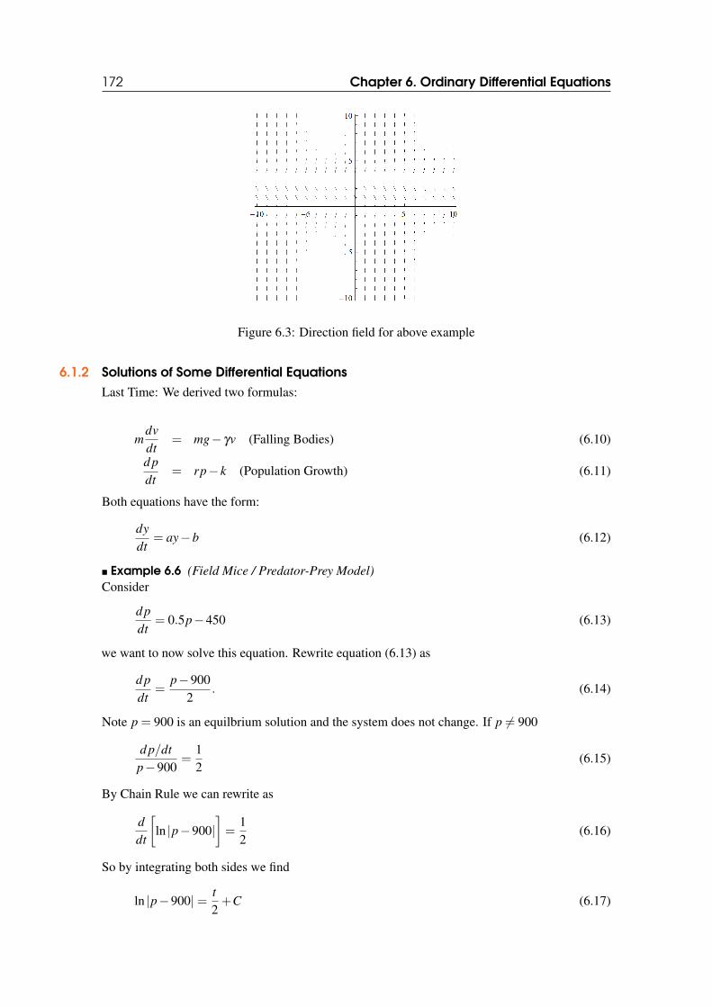
172 Chapter 6. Ordinary Differential Equations
Figure 6.3: Direction field for above example
6.1.2 Solutions of Some Differential EquationsLast Time: We derived two formulas:
mdvdt
= mg− γv (Falling Bodies) (6.10)
d pdt
= rp− k (Population Growth) (6.11)
Both equations have the form:
dydt
= ay−b (6.12)
Example 6.6 (Field Mice / Predator-Prey Model)Consider
d pdt
= 0.5p−450 (6.13)
we want to now solve this equation. Rewrite equation (6.13) as
d pdt
=p−900
2. (6.14)
Note p = 900 is an equilbrium solution and the system does not change. If p 6= 900
d p/dtp−900
=12
(6.15)
By Chain Rule we can rewrite as
ddt
[ln |p−900|
]=
12
(6.16)
So by integrating both sides we find
ln |p−900|= t2+C (6.17)

6.1 Introduction to ODEs 173
Therefore,
p = 900+Cet/2 (6.18)
Thus we have infinitely many solutions where a different arbitrary constant C produces a differentsolution. What if the initial population of mice was 850. How do we account for this?
Definition 6.1.4 The additional condition, p(0) = 850, that is used to determine C is an exampleof an initial condition.
Definition 6.1.5 The differential equation together with the initial condition form the initialvalue problem
Consider the general problem
dydt
= ay−b (6.19)
y(0) = y0 (6.20)
The solution has the form
y = (b/a)+ [y0− (b/a)]eat (6.21)
when a 6= 0 this contains all possible solutions to the general equation and is thus called the generalsolution The geometric representation of the general solution is an infinite family of curves calledintegral curves.
Example 6.7 (Dropping a ball) System under consideration:
dvdt
= 9.8− v5
(6.22)
v(0) = 0 (6.23)
From the formula above we have
v =(−9.8−1/5
)+
[0− −9.8−1/5
]e−
t5 (6.24)
and the general solution is
v = 49+Ce−t/5 (6.25)
with the I.C. C =−49.
6.1.3 Classifications of Differential EquationsLast Time: We solved some basic differential equations, discussed IVPs, and defined the generalsolution.
Now we want to classify two main types of differential equations.
Definition 6.1.6 If the unknown function depends on a single independent variable where onlyordinary derivatives appear, it is said to be an ordinary differential equation. Example
y′(x) = xy (6.26)

174 Chapter 6. Ordinary Differential Equations
Definition 6.1.7 If the unknown function depends on several variables, and the derivatives arepartial derivatives it is said to be a partial differential equation.
One can also have a system of differential equations
dx/dt = ax−αxy (6.27)
dy/dt = −cy+ γxy (6.28)
Note: Questions from this section are common on exams.
Definition 6.1.8 The order of a differential equation is the order of the highest derivative thatappears in the equation.
Ex 1: y′′′+2ety′′+ yy′ = 0 has order 3.Ex 2: y(4)+(y′)2 +4y′′′ = 0 has order 4. Look at derivatives not powers.
Another way to classify equations is whether they are linear or nonlinear:
Definition 6.1.9 A differential equation is said to be linear if F(t,y,y′,y′′, ...,y(n)) = 0 is alinear function in the variables y,y′,y′′, ...,y(n). i.e. none of the terms are raised to a power orinside a sin or cos.
Example 6.8 a) y′+ y = 2b) y′′ = 4y−6c) y(4)+3y′+ sin(t)y
Definition 6.1.10 An equation which is not linear is nonlinear.
Example 6.9 a) y′+ t4y2 = 0b) y′′+ sin(y) = 0c) y(4)− tan(y)+(y′′′)3 = 0
Example 6.10 d2θ
dt2 + gL sin(θ) = 0.
The above equation can be approximated by a linear equation if we let sin(θ) = θ . This pro-cess is called linearization.
Definition 6.1.11 A solution of the ODE on the interval α < t < β is a function φ that satisfies
φ(n)(t) = f [t,φ(t), ...,φ (n−1)(t)] (6.29)
Common Questions:1. (Existence) Does a solution exist? Not all Initial Value Problems (IVP) have solutions.
2. (Uniqueness) If a solution exists how many are there? There can be none, one or infinitely manysolutions to an IVP.
3. How can we find the solution(s) if they exist? This is the key question in this course. Wewill develop many methods for solving differential equations the key will be to identify whichmethod to use in which situation.

6.2 Separable Equations 175
6.2 Separable Equations
In general, we want to solve first order differential equations of the form
dydt
= f (t,y). (6.30)
We begin with equations that have a special form referred to as separable equations of the form
dydx
= f (y)g(x) (6.31)
The General Solution Method:
Step 1: (Separate)1
f (y)dy = g(x)dx (6.32)
Step 2: (Integrate)∫ 1
f (y)dy =
∫g(x)dx (6.33)
Step 3: (Solve for y) F(y) = G(x)+ c (6.34)
Note only need a constant of integration of one side, could just combine the constants we get oneach side. Also, we only solve for y if it is possible, if not leave in implicit form.
Definition 6.2.1 An equilibrium solution is the value of y which makes dy/dx = 0, y remainsthis constant forever.
Example 6.11 (Newton’s Law of Cooling) Consider the ODE, where E is a constant:
dBdt
= κ(E−B) (6.35)
with initial condition (IC) B(0) = B0. This is separable
∫ dBE−B
=∫
κdt (6.36)
− ln |E−B| = κt + c (6.37)
E−B = e−κt+c = Ae−κt (6.38)
B(t) = E−Ae−κt (6.39)
B(0) = E−A (6.40)
A = E−B0 (6.41)
B(t) = E− E−B0
eκt (6.42)
Example 6.12
dydt
= 6y2x, y(1) =13. (6.43)

176 Chapter 6. Ordinary Differential Equations
Separate and Solve:
∫ dyy2 =
∫6xdx (6.44)
−1y
= 3x2 + c (6.45)
y(1) = 1/3 (6.46)
−3 = 3(1)+ c⇒ c =−6 (6.47)
−1y
= 3x2−6 (6.48)
y(x) =1
6−3x2 (6.49)
What is the interval of validity for this solution? Problem when 6−3x2 = 0 or when x =±√
2.So possible intervals of validity: (−∞,−
√2),(−
√2,√
2),(√
2,∞). We want to choose the onecontaining the initial value for x, which is x = 1, so the interval of validity is (−
√2,√
2).
Example 6.13
y′ =3x2 +2x−4
2y−2, y(1) = 3 (6.50)
There are no equilibrium solutions.
∫2y−2dy =
∫3x2 +2x−4dx (6.51)
y2−2y = x3 + x2−4x+ c (6.52)
y(1) = 3⇒ c = 5 (6.53)
y2−2y+1 = x3 + x2−4x+6 (Complete the Square) (6.54)
(y−1)2 = x3 + x2−4x+6 (6.55)
y(x) = 1±√
x3 + x2−4x+6 (6.56)
There are two solutions we must choose the appropriate one. Use the IC to determine only thepositive solution is correct.
y(x) = 1+√
x3 + x2−4x+6 (6.57)
We need the terms under the square root to be positive, so the interval of validity is values of xwhere x3 + x2−4x+6≥ 0. Note x = 1 is in here so IC is in interval of validity.
Example 6.14
dydx
=xy3
1+ x2 , y(0) = 1 (6.58)

6.2 Separable Equations 177
One equilibrium solution, y(x) = 0, which is not our case (since it does not meet the IC). Soseparate:∫ dy
y3 =∫ x
1+ x2 dx (6.59)
− 12y2 =
12
ln(1+ x2)+ c (6.60)
y(0) = 1⇒ c =−12
(6.61)
y2 =1
1− ln(1+ x2)(6.62)
y(x) =1√
1− ln(1+ x2)(6.63)
Determine the interval of validity. Need
ln(1+ x2)< 1⇒ x2 < e−1 (6.64)
So the interval of validity is −√
e−1 < x <√
e−1.
Example 6.15
dydx
=y−1x2 +1
(6.65)
The equilibrium solution is y(x) = 1 and our IC is y(0) = 1, so in this case the solution is theconstant function y(s) = 1.
Example 6.16
(Review IBP)dydt
= ey−t sec(y)(1+ t2), y(0) = 0 (6.66)
Separate by rewriting, and using Integration By Parts (IBP)
dydt
=eye−t
cos(y)(1+ t2) (6.67)∫
e−y cos(y)dy =∫
e−t(1+ t2)dt (6.68)
e−y
2(sin(y)− cos(y)) = −e−t(t2 +2t +3)+
52
(6.69)
Won’t be able to find an explicit solution so leave in implicit form. In the implicit form it is difficultto find the interval of validity so we will stop here.
Example 6.17 Solve the differential equation xy′ = y+1.
Solution: Separate variables
y′
y+1=
1x
Write y′ = dy/dx and Rearrangedy
y+1=
dxx
Integrate both sides∫ 1
y+1dy =
∫ 1x
dx
Simplify ln(y+1) = ln(x)+C
Let C = ln(a) for constant a ln(y+1) = ln(x)+ ln(a) = ln(ax)
put both sides into the exponential function y+1 = ax.

178 Chapter 6. Ordinary Differential Equations
Thus, we have a family of solution y = ax−1. One curve for each value of the constant a. This ismore commonly referred to as the general solution. Finding a particular solution means choosinga value of a so that one curve remains.
6.3 Linear First-Order Equations, Method of Integrating FactorsConsider the general equation
dydt
+ p(t)y = g(t) (6.70)
We said in Chapter 1 if p(t) and g(t) are constants we can solve the equation explicitly. Unfortu-nately this is not the case when they are not constants. We need the method of integrating factordeveloped by Leibniz, who also invented calculus, where we multiply (6.70) by a certain functionµ(t), chosen so the resulting equation is integrable. µ(t) is called the integrating factor. Thechallenge of this method is finding it.
Summary of Method:1. Rewrite the equation as (MUST BE IN THIS FORM)
y′+ay = f (6.71)
2. Find an integrating factor, which is any function
µ(t) = e∫
a(t)dt . (6.72)
3. Multiply both sides of (6.71) by the integrating factor.
µ(t)y′+aµ(t)y = f µ(t) (6.73)
4. Rewrite as a derivative
(µy)′ = µ f (6.74)
5. Integrate both sides to obtain
µ(t)y(t) =∫
µ(t) f (t)dt +C (6.75)
and thus
y(t) =1
µ(t)
∫µ(t) f (t)dt +
Cµ(t)
(6.76)
Now lets see some examples:
Example 6.18 Find the general solution of
y′ = y+ e−t (6.77)
Step 1:
y′− y = et (6.78)
Step 2:
µ(t) = e−∫
1dt = e−t (6.79)

6.3 Linear First-Order Equations, Method of Integrating Factors 179
Step 3:
e−t(y′− y) = e−2t (6.80)
Step 4:
(e−ty)′ = e−2t (6.81)
Step 5:
e−ty =∫
e−2tdt =−12
e−2t +C (6.82)
Solve for y
y(t) =−12
e−t +Cet (6.83)
Example 6.19 Find the general solution of
y′ = ysin t +2te−cos t (6.84)
and y(0) = 1.Step 1:
y′− ysin t = 2te−cos t (6.85)
Step 2:
µ(t) = e−∫
sin tdt = ecos t (6.86)
Step 3:
ecos t(y′− ysin t) = 2t (6.87)
Step 4:
(ecos ty)′ = 2t (6.88)
Step 5:
ecos ty = t2 +C (6.89)
So the general solution is:
y(t) = (t2 +C)e−cos t (6.90)
With IC
y(t) = (t2 + e)e−cos t (6.91)

180 Chapter 6. Ordinary Differential Equations
Example 6.20 Find General Solution to
y′ = y tan t + sin t (6.92)
with y(0) = 2. Note Integrating factor
µ(t) = e−∫
tandt = eln(cos t) = cos t (6.93)
Final Answer
y(t) =−cos t2
+5
2cos t(6.94)
Example 6.21 Solve
2y′+ ty = 2 (6.95)
with y(0) = 1. Integrating Factor
µ(t) = et2/4 (6.96)
Final Answer
y(t) = e−t2/4∫ t
0es2/4ds+ e−t2/4. (6.97)
6.3.1 REVIEW: Integration By PartsThis is the most important integration technique learned in Calculus 2. We will derive the method.Consider the product rule for two functions of t.
ddt
[uv]= u
dvdt
+ vdudt
(6.98)
Integrate both sides from a to b
uv∣∣∣∣ba=∫ b
au
dvdt
+∫ b
av
dudt
(6.99)
Rearrange the resulting terms
∫ b
au
dvdt
= uv∣∣∣∣ba−∫ b
av
dudt
(6.100)
Practicing this many times will be helpful on the homework. Consider two examples.
Example 6.22 Find the integral∫ 9
1 ln(t)dt. First define u,du,dv, and v.
u = ln(t) dv = dt (6.101)
du =1t
dt v = t (6.102)

6.3 Linear First-Order Equations, Method of Integrating Factors 181
Thus ∫ 9
1ln(t)dt = t ln(t)
∣∣∣∣91−∫ 9
11dt (6.103)
= 9ln(9)− t∣∣∣∣91
(6.104)
= 9ln(9)−9+1 (6.105)
= 9ln(9)−8 (6.106)
Example 6.23 Find the integral∫
ex cos(x)dx. First define u,du,dv, and v.
u = cos(x) dv = exdx (6.107)
du =−sin(x)dx v = ex (6.108)
Thus ∫ex cos(x)dx = ex cos(x)−
∫ex sin(x)dx (6.109)
Do Integration By Parts Again
u = sin(x) dv = exdx (6.110)
du = cos(x)dx v = ex (6.111)
So ∫ex cos(x)dx = ex cos(x)−
∫ex sin(x)dx (6.112)
= ex cos(x)+ ex sin(x)−∫
ex cos(x)dx (6.113)
2∫
ex cos(x)dx = ex(cos(x)+ sin(x))
(6.114)∫ex cos(x)dx =
12
ex(cos(x)+ sin(x))+C (6.115)
Notice when we do not have limits of integration we need to include the arbitrary constant ofintegration C.
6.3.2 Modeling With First Order EquationsLast Time: We solved separable ODEs and now we want to look at some applications to real worldsituations
There are two key questions to keep in mind throughout this section:1. How do we write a differential equation to model a given situation?2. What can the solution tell us about that situation?
Example 6.24 (Radioactive Decay)
dNdt
=−λN(t), (6.116)

182 Chapter 6. Ordinary Differential Equations
where N(t) is the number of atoms of a radioactive isotope and λ > 0 is the decay constant. Theequation is separable, and if the initial data is N(0) = N0, the solution is
N(t) = N0e−λ t . (6.117)
so we can see that radioactive decay is exponential.
Example 6.25 (Newton’s Law of Cooling) If we immerse a body in an environment with aconstant temperature E, then if B(t) is the temperature of the body we have
dBdt
= κ(E−B), (6.118)
where κ > 0 is a constant related to the material of the body and how it conducts heat. This equationis separable. We solved it before with the initial condition B(0) = B0 to get
B(t) = E− E−B0
eκt . (6.119)
Approaches to writing down a model describing a situation:1. Remember the derivative is the rate of change. It’s possible that the description of the problemtells us directly what the rate of change is. Newton’s Law of Cooling tells us the rate of change ofthe body’s temperature was proportional to the difference in temperature between the body and theenvironment. All we had to do was set the relevant terms equal.
2. There are also cases where we are not explicitly given the formula for the rate of change.But we may be able to use the physical description to define the rate of change and then set thederivative equal to that. Note: The derivative = increase - decrease. This type of thinking is onlyapplicable to first order equations since higher order equations are not formulated as rate of changeequals something.
3. We may just be adapting a known differential equation to a particular situation, i.e. New-ton’s Second Law F = ma. It is either a first or second order equation depending on if you defineit for position for velocity. Combine all forces and plug in value for F to yield the differentialequation. Used for falling bodies, harmonic motion, and pendulums.
4. The last possibility is to determine two different expressions for the same quantity and setthe equal to derive a differential equation. Useful when discussing PDEs later in the course.
The first thing one must do when approaching a modeling problem is determining which ofthe four situations we are in. It is crucial to practice this identification now it will be useful onexams and later sections. Secondly, your differential equation should not depend on the initialcondition. The IC only tells the starting position and should not effect how a system evolves.
Type I: (Interest)
Suppose there is a bank account that gives r% interest per year. If I withdraw a constant wdollars per month, what is the differential equation modeling this?
Ans: Let t be time in years, and denote the balance after t years as B(t). B′(t) is the rate ofchange of my account balance from year to year, so it will be the difference between the amount

6.3 Linear First-Order Equations, Method of Integrating Factors 183
added and the amount withdrawn. The amount added is interest and the amount withdrawn is 12w.Thus
B′(t) =r
100B(t)−12w (6.120)
This is a linear equation, so we can solve by integrating factor. Note: UNITS ARE IMPORTANT,w is withdrawn each month, but 12w is withdrawn per year.
Example 6.26 Bill wants to take out a 25 year loan to buy a house. He knows that he can affordmaximum monthly payments of $400. If the going interest rate on housing loans is 4%, what is thelargest loan Bill can take out so that he will be able to pay it off in time?
Ans: Measure time t in years. The amount Bill owes will be B(t). We want B(25) = 0. The4% interest rate will take the form of .04B added. He can make payments of 12×400 = 4800 eachyear. So the IVP will be
B′(t) = .04B(t)−4800, B(25) = 0 (6.121)
This is a linear equation in standard form, use integrating factor
B′(t)− .04B(t) = −4800 (6.122)
µ(t) = e∫−.04dt = e−.04t (6.123)
(e−4
100 tB(t))′ = −4800e−4
100 t (6.124)
e−4
100 tB(t) = −4800∫
e−4
100 tdt = 120000e−4
100 t + c (6.125)
B(t) = 120000+ ce4
100 t (6.126)
B(25) = 0 = 120000+ ce⇒ c =−120000e−1 (6.127)
B(t) = 120000−120000e4
100 (t−25) (6.128)
We want the size of the loan, which is the amount Bill begins with B(0):
B(0) = 120000−120000e−1 = 120000(1− e−1) (6.129)
Type II: (Mixing Problems)
Out
In
We have a mixing tank containing some liquid inside. Contaminant is being added to the tank atsome constant rate and the mixed solution is drained out at a (possibly different) rate. We will wantto find the amount of contaminant in the tank at a given time.How do we write the DE to model this process? Let P(t) be the amount of pollutant (Note: Amount

184 Chapter 6. Ordinary Differential Equations
of pollutant, not the concentration) in the tank at time t. We know the amount of pollutant that isentering and leaving the tank each unit of time. So we can use the second approach
Rate of Change ofP(t) = Rate of entry of contaminant−Rate of exit of contaminant (6.130)
The rate of entry can be defined in different ways. 1. Directly adding contaminant i.e. pipe addingfood coloring to water. 2. We might be adding solution with a known concentration of contaminantto the tank (amount = concentration x volume).What is the rate of exit? Suppose that we are draining the tank at a rate of rout . The amount ofcontaminant leaving the tank will be the amount contained in the drained solution, that is givenby rate x concentration. We know the rate, and we need the concentration. This will just be theconcentration of the solution in the tank, which is in turn given by the amount of contaminant inthe tank divided by the volume.
Rate of exit of contaminant = Rate of drained solution× Amount of ContaminantVolume of Tank
(6.131)
or
Rate of exit of contaminant = routP(t)V (t)
. (6.132)
What is V (t)? The Volume is decreasing by rout at each t. Is there anything being added to thevolume? That depends if we are adding some solution to the tank at a certain rate rin, that willadd to the in-tank volume. If we directly add contaminant not in solution, nothing is added. Sodetermine which situation by reading the problem. In the first case if the initial volume is V0, we’llget V (t) =V0 + t(rin− rout), and in the second, V (t) =V0− trout .
Example 6.27 Suppose a 120 gallon well-mixed tank initially contains 90 lbs. of salt mixedwith 90 gal. of water. Salt water (with a concentration of 2 lb/gal) comes into the tank at a rate of4 gal/min. The solution flows out of the tank at a rate of 3 gal/min. How much salt is in the tankwhen it is full?
Ans: We can immediately write down the expression for volume V (t). How much liquid isentering each minute? 4 gallons. How much is leaving the tank in the same minute? 3 gallons. Soeach minute the Volume increases by 1 gallon, and we have V (t) = 90+(4−3)t = 90+ t. Thistells us the tank will be full at t = 30.We let P(t) be the amount of salt (in pounds) in the tank at time t. Ultimately, we want to determineP(30), since this is when the tank will be full. We need to determine the rates at which salt isentering and leaving the tank. How much salt is entering? 4 gallons of salt water enter the tankeach minute, and each of those gallons has 2lb. of salt dissolved in it. Hence we are adding 8 lbs.of salt to the tank each minute. How much is exiting the tank? 3 gallons leave each minute, and theconcentration in each of those gallons is P(t)/V (t). Recall
Rate of Change ofP(t) = Rate of entry of contaminant−Rate of exit of contaminant
(6.133)
Rate of exit of contaminant = Rate of drained solution× Amount of ContaminantVolume of Tank
(6.134)
dPdt
= (4gal/min)(2lb/gal)− (3gal/min)(P(t)lb
V (t)gal) = 8− 3P(t)
90+ t(6.135)

6.3 Linear First-Order Equations, Method of Integrating Factors 185
This is the ODE for the salt in the tank, what is the IC? P(0) = 90 as given by the problem. Now wehave an IVP so solve (since linear) using integrating factor
dPdt
+3
90+ tP(t) = 8 (6.136)
µ(t) = e∫ 3
90+t dt = e3ln(90+t) = (90+ t)3 (6.137)
((90+ t)3P(t))′ = 8(90+ t)3 (6.138)
(90+ t)3P(t) =∫
8(90+ t)3dt = 2(90+ t)4 + c (6.139)
P(t) = 2(90+ t)+c
(90+ t)3 (6.140)
P(0) = 90 = 2(90)+c
903 ⇒ c =−(90)4 (6.141)
P(t) = 2(90+ t)− 904
(90+ t)3 (6.142)
Remember we wanted P(30) which is the amount of salt when the tank is full. So
P(30) = 240− 904
1203 = 240−90(34)3 = 240−90(
2764
). (6.143)
We could ask for amount of salt at anytime before overflow and all would be the same besides laststep where we replace 30 with the time wanted.
Exercise: What is the concentration of the tank when the tank is full?
Example 6.28 A full 20 liter tank has 30 grams of yellow food coloring dissolved in it. If ayellow food coloring solution (with concentration of 2 grams/liter) is piped into the tank at a rate of3 liters/minute while the well mixed solution is drained out of the tank at a rate of 3 liters/minute,what is the limiting concentration of yellow food coloring solution in the tank?
Ans: The ODE would be
dPdt
= (3L/min)(2g/L)− (3L/min)P(t)gV (t)L
= 6− 3P20
(6.144)
Note that volume is constant since we are adding and removing the same amount at each time step.Use the method of integrating factor.
µ(t) = e∫ 3
20 dt = e320 t (6.145)
(e320 tP(t))′ = 6e
320 t (6.146)
e3
20 tP(t) =∫
6e320 tdt = 40e
320 t + c (6.147)
P(t) = 40+c
e320 t
(6.148)
P(0) = 20 = 40+ c⇒ c =−20 (6.149)
P(t) = 40− 20
e320 t
. (6.150)
Now what will happen to the concentration in the limit, or as t → ∞. We know the volume willalways be 20 liters.
limt→∞
P(t)V (t)
= limt→∞
40−20e−320 t
20= 2 (6.151)

186 Chapter 6. Ordinary Differential Equations
So the limiting concentration is 2g/L. Why does this make physical sense? After a period of timethe concentration of the mixture will be exactly the same as the concentration of the incomingsolution. It turns out that the same process will work if the concentration of the incoming solutionis variable.
Example 6.29 A 150 gallon tank has 60 gallons of water with 5 pounds of salt dissolved in it.Water with a concentration of 2+ cos(t) lbs/gal comes into the tank at a rate of 9 gal/hr. If the wellmixed solution leaves the tank at a rate of 6 gal/hour, how much salt is in the tank when it overflows?
Ans: The only difference is the incoming concentration is variable. Given the Volume startsat 600 gal and increases at a rate of 3 gal/min
dPdt
= 9(2+ cos(t))− 6P60+3t
(6.152)
Our IC is P(0) = 5 and use the method of integrating factor
µ(t) = e∫ 6
60+3t dt = e2ln(20+t) = (20+ t)2. (6.153)
((20+ t)2P(t))′ = 9(2+ cos(t))(20+ t)2 (6.154)
(20+ t)2P(t) =∫
9(2+ cos(t))(20+ t)2dt (6.155)
= 9(23(20+ t)3 +(20+ t)2 sin(t)+2(20+ t)cos(t)−2sin(t))+ c(6.156)
P(t) = 9(23(20+ t)+ sin(t)+
2cos(t)20+ t
− 2sin(t)(20+ t)2 )+
c(20+ t)2 (6.157)
P(0) = 5 = 9(23(20)+
220
)+c
400= 120+
910
+c
400(6.158)
c = −46360 (6.159)
We want to know how much salt is in the tank when it overflows. This happens when the volumehits 150, or at t = 30.
P(30) = 300+9sin(30)+18cos(30)
50− 18sin(30)
2500− 46360
2500(6.160)
So P(t)≈ 272.63 pounds.
We could make the problem more complicated by assuming that there will be a change in thesituation if the solution ever reached a critical concentration. The process would still be the same,we would just need to solve two different but limited IVPs.
Type III: (Falling Bodies)Lets consider an object falling to the ground. This body will obey Newton’s Second Law of Motion,
mdvdt
= F(t,v) (6.161)
where m is the object’s mass and F is the net force acting on the body. We will look at the situationwhere the only forces are air resistance and gravity. It is crucial to be careful with the signs.Throughout this course downward displacements and forces are positive. Hence the force dueto gravity is given by FG = mg, where g≈ 10m/s2 is the gravitational constant.Air Resistance acts against velocity. If the object is moving up air resistance works downward,always in opposite direction. We will assume air resistance is linearly dependant on velocity (ie

6.4 Existence and Uniqueness 187
FA = αv, where FA is the force due to air resistance). This is not realistic, but it simplifies theproblem. So F(t,v) = FG +FA = 10−αv, and our ODE is
mdvdt
= 10m−αv (6.162)
Example 6.30 A 50 kg object is shot from a cannon straight up with an initial velocity of 10 m/soff the very tip of a bridge. If the air resistance is given by 5v, determine the velocity of the mass atany time t and compute the rock’s terminal velocity.
Ans: Two parts: 1. When the object is moving upwards and 2. When the object is movingdownwards. If we look at the forces it turns out we get the same DE
50v′ = 500−5v (6.163)
The IC is v(0) =−10, since we shot the object upwards. Our DE is linear and we can use integratingfactor
v′+110
v = 10 (6.164)
µ(t) = et
10 (6.165)
(et
10 v(t))′ = 10et
10 (6.166)
et
10 v(t) =∫
10et
10 dt = 100et
10 + c (6.167)
v(t) = 100+c
et
10(6.168)
v(0) = −10 = 100+ c⇒ c =−110 (6.169)
v(t) = 100− 110
et
10. (6.170)
What is the terminal velocity of the rock? The terminal velocity is given by the limit of the velocityas t → ∞, which is 100. We could also have computed the velocity of the rock when it hit theground if we knew the height of the bridge (integrate to get position).
Example 6.31 A 60kg skydiver jumps out of a plane with no initial velocity. Assuming themagnitude of air resistance is given by 0.8|v|, what is the appropriate initial value problem modelinghis velocity?
Ans: Air Resistance is an upward force, while gravity is acting downward. So our force should be
F(t,v) = mg− .8v (6.171)
thus our IVP is
60v′ = 60g− .8v, v(0) = 0 (6.172)
6.4 Existence and UniquenessLast Time: We developed 1st Order ODE models for physical systems and solved them using themethods of Integrating Factor and Separable Equations.
In Section 1.3 we noted three common questions we would be concerned with this semester.

188 Chapter 6. Ordinary Differential Equations
1. (Existence) Given an IVP, does a solution exist?2. (Uniqueness) If a solution exists, is it unique?3. If a solution exists, how do we find it?
We have spent a lot of time on developing methods, now we will spend time on the first twoquestions. Without Solving an IVP, what information can we derive about the existence anduniqueness of solutions? Also we will note strong differences between linear and nonlinearequations.
6.4.1 Linear EquationsWhile we will focus on first order linear equations, the same basic ideas work for higher orderlinear equations.
Theorem 6.4.1 (Fundamental Theorem of Existence and Uniqueness for Linear Equations)Consider the IVP
y′+ p(t)y = q(t), y(t0) = y0. (6.173)
If p(t) and q(t) are continuous functions on an open interval α < t0 < β , then there exists aunique solution to the IVP defined on the interval (α,β ).
R The same result holds for general IVPs. If we have the IVP
y(n)+an−1(t)y(n−1)+ ...+a1(t)y′+a0(t)y = g(t), y(t0) = y0, ...,y(n−1)(t0) = y(n−1)0
(6.174)
then if ai(t) (for i = 0, ...,n−1) and g(t) are continuous on an open interval α < t0 < β , thereexists a unique solution to the IVP defined on the interval (α,β ).
What does Theorem 1 tell us?(1) If the given linear differential equation is nice, not only do we know EXACTLY ONEsolution exists. In most applications knowing a solution is unique is more important thanknowing a solution exists.(2) If the interval (α,β ) is the largest interval on which p(t) and q(t) are continuous, then(α,β ) is the interval of validity to the unique solution guaranteed by the theorem. Thus givena "nice" IVP there is no need to solve the equation to find the interval of validity. The intervalonly depends on t0 since the interval must contain it, but does not depend on y0.
Example 6.32 Without solving, determine the interval of validity for the solution to the followingIVP
(t2−9)y′+2y = ln |20−4t|, y(4) =−3 (6.175)
Ans: If we look at Theorem 1, we need to write our equation in the form given in Theorem 1 (i.e.coefficient of y′ is 1). So rewrite as
y′+2
t2−9=
ln |20−4t|t2−9
(6.176)
Next we identify where either of the two other coefficients are discontinuous. By removing thosepoints we find all intervals of validity. Then the last step is to identify which interval of validitycontains t0.

6.4 Existence and Uniqueness 189
Using the notation in Theorem 1, p(t) is discontinuous when t =±3, since at those points weare dividing by zero. q(t) is discontinuous at t = 5, since the natural log of 0 does not exists (onlydefined on (0,∞)). This yields four intervals of validity where both p(t) and q(t) are continuous
(−∞,−3), (−3,3), (3,5), (5,∞) (6.177)
Notice the endpoints are where p(t) and q(t) are discontinuous, guaranteeing within each intervalboth are continuous. Now all that is left is to identify which interval contains t0 = 4. Thus ourinterval of validity is (3,5).
R The other intervals of validity we found are intervals of validity for the same differentialequation, but for different initial conditions. For example, if our IC was y(2) = 5 then theinterval of validity must contain 2, so the answer would be (−3,3).
What happens if our IC is at one of the bad points where p(t) and q(t) are discontinu-ous? Unfortunately we are unable to conclude anything, since the theorem does not apply.On the other hand we cannot say that a solution does not exist just because the hypothesis arenot met, so the bottom line is that we cannot conclude anything.
6.4.2 Nonlinear EquationsWe saw in the linear case every "nice enough" equation has a unique solution except for if the initialconditions are ill-posed. But even this seemingly simple nonlinear equation
(dtdx
)2 + x2 +1 = 0 (6.178)
has no real solutions.
So we have the following revision of Theorem 1 that applies to nonlinear equations as well.Since this is applied to a broader class the conclusions are expected to be weaker.
Theorem 6.4.2 Consider the IVP
y′ = f (t,y), y(t0) = y0. (6.179)
If f and ∂ f∂y are continuous functions on some rectangle α < t0 < β ,γ < y0 < δ containing the
point (t0,y0), then there is a unique solution to the IVP defined on some interval (a,b) satisfyingα < a < t0 < b≤ β .
OBSERVATION:(1) Unlike Theorem 1, Theorem 2 does not tell us the interval of a unique solution guaranteed byit. Instead, it tells us the largest possible interval that the solution will exist in, we would need toactually solve the IVP to get the interval of validity.(2) For nonlinear differential equations, the value of y0 may affect the interval of validity, as wewill see in a later example. We want our IC to NOT lie on the boundary of a region where f or itspartial derivative are discontinuous. Then we find the largest t-interval on the line y = y0 containingt0 where everything is continuous.
R Theorem 2 refers to partial derivative ∂ f∂y of the function of two variables f (t,y). We will
talk extensively about this later, but for now we treat t as a constant and take a normal

190 Chapter 6. Ordinary Differential Equations
derivative with respect to y. For example
f (t,y) = t2−2y3t, then∂ f∂y
=−6y2t. (6.180)
Example 6.33 Determine the largest possible interval of validity for the IVP
y′ = x ln(y), y(2) = e (6.181)
We have f (x,y) = x ln(y), so ∂ f∂y = x
y . f is discontinuous when y≤ 0, and fy (partial derivative withrespect to y) is discontinuous when y = 0. Since our IC y(2) = e > 0 there is no problem sincey0 is never in the discontinuous region. Since there are no discontinuities involving x, then therectangle is −∞ < x0 < ∞,0 < y0 < ∞. Thus the theorem concludes that the unique solution existssomewhere inside (−∞,∞).
R Note that this basically told us nothing, and nonlinear problems are quite harder to deal withthan linear. What can happen if the conditions of Theorem 2 are NOT met?
Example 6.34 Determine all possible solutions to the IVP
y′ = y13 , y(0) = 0. (6.182)
First note this does not satisfy the conditions of the theorem, since fy =1
3y2/3 is not continuous aty0 = y = 0. Now solve the equation it is separable. Notice the equilibrium solution is y = 0. Thissatisfies the IC, but let’s solve the equation.∫
y−1/3dy =∫
dt (6.183)
32
y2/3 = t + c (6.184)
y(0) = 0 (6.185)
y(t) = ±(23
t)32 (6.186)
(6.187)
The IC does not rule out either of these possibilities, so we end up with three possible solutions(these two and the equilibrium solution y(t)≡ 0).
6.5 Other Methods for First-Order Equations6.5.1 Autonomous Equations with Population Dynamics
First order differential equations relate the slope of a function to the values of the function and theindependent variable. We can visualize this using direction fields. This in principle can be verycomplicated and it might be hard to determine which initial values correspond to which outcomes.However, there is a special class of equations, called autonomous equations, where this process issimplified. The first thing to note is autonomous equations do not depend on t
y′ = f (y) (6.188)
R Notice that all autonomous equations are separable.
6.5 Other Methods for First-Order Equations 191
What we need to know to study the equation qualitatively is which values of y make y′ zero,positive, or negative. The values of y making y′ = 0 are the equilibrium solutions. They areconstant solutions and are indicated on the ty-plane by horizontal lines.
After we establish the equilibrium solutions we can study the positivity of f (y) on the interme-diate intervals, which will tell us whether the equilibrium solutions attract nearby initial conditions(in which case they are called asymptotically stable), repel them (unstable), or some combinationof them (semi-stable).
Example 6.35 Consider
y′ = y2− y−2 (6.189)
Start by finding the equilibrium solutions, values of y such that y′ = 0. In this case we need tosolve y2− y−2 = (y−2)(y+1) = 0. So the equilibrium solutions are y =−1 and y = 2. Thereare constant solutions and indicated by horizontal lines. We want to understand their stability. Ifwe plot y2− y− 2 versus y, we can see that on the interval (−∞,−1), f (y) > 0. On the interval(−1,2), f (y)< 0 and on (2,∞), f (y)> 0. Now consider the initial condition.
(1) If the IC y(t0) = y0 <−1,y′ = f (y)> 0 and y(t) will increase towards -1.(2) If the IC−1< y0 < 2,y′= f (y)< 0, so the solution will decrease towards -1. Since the solutionsbelow -1 go to -1 and the solutions above -1 go to -1, we conclude y(t) =−1 is an asymptoticallystable equilibrium.(3) If y0 > 2,y′ = f (y)> 0, so the solution increases away from 2. So at y(t) = 2 above and belowsolutions move away so this is an unstable equilibrium.
Example 6.36 Consider
y′ = (y−4)(y+1)2 (6.190)
The equilibrium solutions are y =−1 and y = 4. To classify them, we graph f (y) = (y−4)(y+1)2.(1) If y <−1, we can see that f (y)< 0, so solutions starting below -1 will tend towards −∞.(2) If −1 < y0 < 4, f (y) < 0, so solutions starting here tend downwards to -1. So y(t) = 1 issemistable.(3) If y > 4, f (y)> 0, solutions starting above 4 will asymptotically increase to ∞, so y(t) = 4 isunstable since no nearby solutions converge to it.
Populations
The best examples of autonomous equations come from population dynamics. The most naivemodel is the "Population Bomb" since it grows without any deaths
P′(t) = rP(t) (6.191)
with r > 0. The solution to this differential equation is P(t) = P0ert , which indicates that thepopulation would increase exponentially to ∞. This is not realistic at all.
A better and more accurate model is the "Logistic Model"
P′(t) = rP(1− PN) = rP− r
NP2 (6.192)
where N > 0 is some constant. With this model we have a birth rate of rP and a mortality rate of

192 Chapter 6. Ordinary Differential Equations
rN P2. The equation is separable so let’s solve it.
dPP(1− P
N )= rdt (6.193)∫
(1P+
1/N1−P/N
)dP =∫
rdt (6.194)
ln |P|− ln |1− PN| = rt + c (6.195)
P1− P
N
= Aert (6.196)
P = Aert =1N
AertP (6.197)
P(t) =Aert
1+ AN ert
=AN
Ne−rt +A(6.198)
if P(0) = P0, then A = P0NN−P0
to yield
P(t) =P0N
(N−P0)e−rt +P0(6.199)
In its present form its hard to analyze what is going on so let’s apply the methods from the firstsection to analyze the stability.
Looking at the logistic equation, we can see that our equilibrium solutions are P = 0 and P = N.Graphing f (P) = rP(1− N
P ), we see that(1) If P < 0, f (P)< 0(2) If 0 < P < N, f (P)> 0(3) If P > N, f (P)< 0Thus 0 is unstable while while N is asymptotically stable, so we can conclude for initial populationP0 > 0
limt→∞
P(t) = N (6.200)
So what is N? It is the carrying capacity for the environment. If the population exists, it will growtowards N, but the closer it gets to N the slower the population will grow. If the population startsoff greater then the carrying capacity for the environment P0 > N, then the population will die offuntil it reaches that stable equilibrium position. And if the population starts off at N, the births anddeaths will balance out perfectly and the population will remain exactly at P0 = N.
Note: It is possible to construct similar models that have unstable equilibria above 0.
Exercise 6.1 Show that the equilibrium population P(t) = N is unstable for the autonomousequation
P′(t) = rP(PN−1). (6.201)

6.5 Other Methods for First-Order Equations 193
6.5.2 Bernoulli EquationsThe Bernoulli equation is a special first order equation of the form:
y′+Py = Qyn, (6.202)
where P,Q are functions of x. Even though the equation is not linear, we can reduce it to a linearequation with the following transformation: z = y1−n where by Chain Rule z′ = (1−n)y−ny′. Nowmultiply (6.202) by (1−n)y−n to find
(1−n)y−ny′+(1−n)Py1−n = (1−n)Q
z′+(1−n)Pz = (1−n)Q.
We now have a first order linear equation that could be solved using the method of integratingfactor.
6.5.3 Exact EquationsThe final category of first order differential equations we will consider are Exact Equations. Thesenonlinear equations have the form
M(x,y)+N(x,y)dydx
= 0 (6.203)
where y = y(x) is a function of x and find the
∂M∂y
=∂N∂x
(6.204)
where these two derivatives are partial derivatives.
Multivariable DifferentiationIf we want a partial derivative of f (x,y) with respect to x we treat y as a constant and differentiatenormally with respect to x. On the other hand, if we want a partial derivative of f (x,y) with respectto y we treat x as a constant and differentiate normally with respect to y.
Example 6.37 Let f (x,y) = x2y = y2. Then
∂ f∂x
= 2xy (6.205)
∂ f∂y
= x2 +2y. (6.206)
Example 6.38 Let f (x,y) = ysin(x)
∂ f∂x
= ycos(y) (6.207)
∂ f∂y
= sin(x) (6.208)
We also need the crucial tool of the multivariable chain rule. If we have a function Φ(x,y(x))depending on some variable x and a function y depending on x, then
dΦ
dx=
∂Φ
∂x+
∂Φ
∂ydydx
= Φx +Φyy′ (6.209)

194 Chapter 6. Ordinary Differential Equations
Solving Exact EquationsStart with an example to illustrate the method.
Example 6.39 Consider
2xy−9x2 +(2y+ x2 +1)dydx
= 0 (6.210)
The first step in solving an exact equation is to find a certain function Φ(x,y). Finding Φ(x,y) ismost of the work. For this example it turns out
Φ(x,y) = y2 +(x2 +1)y−3x3 (6.211)
Notice if we compute the partial derivatives of Φ, we obtain
Φx(x,y) = 2xy−9x2 (6.212)
Φy(x,y) = 2y+ x2 +1. (6.213)
Looking back at the differential equation, we can rewrite it as
Φx +Φydydx
= 0. (6.214)
Thinking back to the chain rule we can express as
dΦ
dx= 0 (6.215)
Thus if we integrate, Φ = c, where c is a constant. So the general solution is
y2 +(x2 +1)y−3x3 = c (6.216)
for some constant c. If we had an initial condition, we could use it to find the particular solution tothe initial value problem.
Let’s investigate the last example further. An exact equation has the form
M(x,y)+N(x,y)dydx
= 0 (6.217)
with My(x,y) = Nx(x,y). The key is to construct Φ(x,y) such that the DE turns into
dΦ
dx= 0 (6.218)
by using the multivariable chain rule. Thus we require Φ(x,y) satisfy
Φx(x,y) = M(x,y) (6.219)
Φy(x,y) = N(x,y) (6.220)
R A standard fact from multivariable calculus is that mixed partial derivatives commute. Thatis why we want My = Nx, so My = Φxy and Nx = Φyx, and so these should be equal for Φ toexist. Make sure you check the function is exact before wasting time on the wrong solutionprocess.
6.5 Other Methods for First-Order Equations 195
Once we have found Φ, then dΦ
dx = 0, and so
Φ(x,y) = c (6.221)
yielding an implicit general solution to the differential equation.So the majority of the work is computing Φ(x,y). How can we find this desired function, let’s
retry Example 3, filling in the details.
Example 6.40 Solve the initial value problem
2xy−9x2 +(2y+ x2 +1)dydx
= 0, y(0) = 2 (6.222)
Let’s begin by checking the equation is in fact exact.
M(x,y) = 2xy−9x2 (6.223)
N(x,y) = 2y+ x2 +1 (6.224)
(6.225)
Then My = 2x = Ny, so the equation is exact.Now how do we find Φ(x,y)? We have Φx = M and Φy = N. Thus we could compute Φ in one
of two ways
Φ(x,y) =∫
Mdx or Φ(x,y) =∫
Ndy. (6.226)
In general it does not usually matter which you choose, one may be easier to integrate than theother. In this case
Φ(x,y) =∫
2xy−9x2dx = x2y−3x3 +h(y). (6.227)
Notice since we only integrate with respect to x we can have an arbitrary function only dependingon y. If we differentiate h(y) with respect to x we still get 0 like an arbitrary constant c. So in orderto have the highest accuracy we take on an arbitrary function of y. Note if we integrated N withrespect to y we would get an arbitrary function of x. DO NOT FORGET THIS!
Now all we need is to find h(y). We know if we differentiate Φ with respect to x, then h(y) willvanish which is unhelpful. So instead differentiate with respect to y, since Φy = N in order to beexact. so any terms in N that aren’t in Φy must be h′(y).
So Φy = x2 +h′(y) and N = x2 +2y+1. Since these are equal we have h′(y) = 2y+1, an so
h(y) =∫
h′(y)dy = y2 + y (6.228)
R We will drop the constant of integration we get from integrating h since it will combine withthe constant c that we get in the solution process.
Thus, we have
Φ(x,y) = x2y−3x3 + y2 + y = y2 +(x2 +1)y−3x3, (6.229)
which is precisely the Φ that we used in Example 3. Observe
dΦ
dx= 0 (6.230)

196 Chapter 6. Ordinary Differential Equations
and thus Φ(x,y) = y2 +(x2 +1)y−3x3 = c for some constant c. To compute c, we’ll use our initialcondition y(0) = 2
22 +2 = c⇒ c = 6 (6.231)
and so we have a particular solution of
y2 +(x2 +1)y−3x3 = 6 (6.232)
This is a quadratic equation in y, so we can complete the square or use quadratic formula to get anexplicit solution, which is the goal when possible.
y2 +(x2 +1)y−3x3 = 6 (6.233)
y2 +(x2 +1)y+(x2 +1)2
4= 6+3x3 +
(x2 +1)2
4(6.234)
(y+x2 +1
2)2 =
x4 +12x3 +2x2 +254
(6.235)
y(x) =−(x2 +1)±
√x4 +12x3 +2x2 +25
2(6.236)
Now we use the initial condition to figure out whether we want the + or − solution. Since y(0) = 2we have
2 = y(0) =−1±
√25
2=−1±5
2= 2,−3 (6.237)
Thus we see we want the + so our particular solution is
y(x) =−(x2 +1)+
√x4 +12x3 +2x2 +25
2(6.238)
Example 6.41 Solve the initial value problem
2xy2 +2 = 2(3− x2y)y′, y(−1) = 1. (6.239)
First we need to put it in the standard form for exact equations
2xy2 +2−2(3− x2y)y′ = 0. (6.240)
Now, M(x,y) = 2xy2 +2 and N(x,y) =−2(3− x2y). So My = 4xy = Nx and the equation is exact.The next step is to compute Φ(x,y). We choose to integrate N this time
Φ(x,y) =∫
Ndy =∫
2x2y−6dy = x2y2−6y+h(x). (6.241)
To find h(x), we compute Φx = 2xy2 + h′(x) and notice that for this to be equal to M, h′(x) = 2.Hence h(x) = 2x and we have an implicit solution of
x2y2−6y+2x = c. (6.242)
Now, we use the IC y(−1) = 1:
1−6−2 = c⇒ c =−7 (6.243)

6.5 Other Methods for First-Order Equations 197
So our implicit solution is
x2y2−6y+2x+7 = 0. (6.244)
Again complete the square or use quadratic formula
y(x) =6±√
36−4x2(2x+7)2x2 (6.245)
=3±√
9−2x3−7x2
x2 (6.246)
and using the IC, we see that we want − solution, so the explicit particular solution is
y(x) =3−√
9−2x3−7x2
x2 (6.247)
Example 6.42 Solve the IVP
2tyt2 +1
−2t− (4− ln(t2 +1))y′ = 0, y(2) = 0 (6.248)
and find the solution’s interval of validity.This is already in the right form. Check if it is exact, M(t,y) = 2ty
t2+1 − 2t and N(t,y) =ln(t2 +1)−4, so My =
2tt2+1 = Nt . Thus the equation is exact. Now compute Φ(x,y). Integrate M
Φ =∫
Mdt =∫ 2ty
t2 +1dt = y ln(t2 +1)− t2 +h(y). (6.249)
Φy = ln(t2 +1)+h′(y) = ln(t2 +1)−4 = N (6.250)
so we conclude h′(y) =−4 and thus h(y) =−4y. So our implicit solution is then
y ln(t2 +1)− t2−4y = c (6.251)
and using the IC we find c =−4. Thus the particular solution is
y ln(t2 +1)− t2−4y =−4 (6.252)
Solve explicitly to obtain
y(x) =t2−4
ln(t2 +1)−4. (6.253)
Now let’s find the interval of validity. We do not have to worry about the natural log sincet2 +1 > 0 for all t. Thus we want to avoid division by 0.
ln(t2 +1)−4 = 0 (6.254)
ln(t2 +1) = 4 (6.255)
t2 = e4−1 (6.256)
t = ±√
e4−1 (6.257)
So there are three possible intervals of validity, we want the one containing t = 2, so (−√
e4−1,√
e4−1).

198 Chapter 6. Ordinary Differential Equations
Example 6.43 Solve
3y3e3xy−1+(2ye3xy +3xy2e3xy)y′ = 0, y(1) = 2 (6.258)
We have
My = 9y2e3xy +9xy3e3xy = Nx (6.259)
Thus the equation is exact. Integrate M
Φ =∫
Mdx =∫
3y3e3xy−1 = y2e3xy− x+h(y) (6.260)
and
Φy = 2ye3xy +3xy2e3xy +h′(y) (6.261)
Comparing Φy to N, we see that they are already identical, so h′(y) = 0 and h(y) = 0. So
y2e3xy− x = c (6.262)
and using the IC gives c = 4e6−1. Thus our implicit particular solution is
y2e3xy− x = 4e6−1, (6.263)
and we are done because we will not be able to solve this explicitly.
6.5.4 Homogeneous EquationsA homogeneous function of x and y of degree n means that a function can be written as xn f (y/x).For example
x3− xy2 = x3[1− (y/x)2]
is a homogeneous function of degree 3. An equation of the form
P(x,y)dx+Q(x,y)dy = 0 (6.264)
where P,Q are homogeneous functions of the same degree and the equation can be rewritten as
y′ =dydx
=−P(x,y)Q(x,y)
= f(y
x
). (6.265)
This suggest that homogeneous equations of this form could be solved by a change of variablesv = y/x or y = xv. After substitution the equation becomes separable! y′ = f (v).
6.6 Second-Order Linear Equations with Constant Coefficients and Zero Right-Hand Side
6.6.1 Basic ConceptsThe example of a second order equation which we have seen many times before is Newton’s SecondLaw when expressed in terms of position s(t) is
md2sdt2 = F(t,s′,s) (6.266)
One of the most basic 2nd order equations is y′′ = −y. By inspection, we might noticethat this has two obvious nonzero solutions: y1(t) = cos(t) and y2(t) = sin(t). But consider9cos(t)−2sin(t)? This is also a solution. Anything of the form y(t) = c1 cos(t)+ c2 sin(t), wherec1 and c2 are arbitrary constants. Every solution if no conditions are present has this form.

6.6 Second-Order Linear Equations with Constant Coefficients and ZeroRight-Hand Side 199 Example 6.44 Find all of the solutions to y′′ = 9y
We need a function whose second derivative is 9 times the original function. What functioncomes back to itself without a sign change after two derivatives? Always think of the exponentialfunction when situations like this arise. Two possible solutions are y1(t) = e3t and y2(t) = e−3t .In fact so are any combination of the two. This is the principal of linear superposition. Soy(t) = c1e3t + c2e−3t are infinitely many solutions.
EXERCISE: Check that y1(t) = e3t and y2(t) = e−3t are solutions to y′′ = 9y.
The general form of a second order linear differential equation is
p(t)y′′+q(t)y′+ r(t)y = g(t). (6.267)
We call the equation homogeneous if g(t) = 0 and nonhomogeneous if g(t) 6= 0.
Theorem 6.6.1 (Principle of Superposition) If y1(t) and y2(t) are solutions to a second orderlinear homogeneous differential equation, then so is any linear combination
y(t) = c1y1(t)+ c2y2(t). (6.268)
This follows from the homogeneity and the fact that a derivative is a linear operator. So givenany two solutions to a homogeneous equation we can find infinitely more by combining them. Themain goal is to be able to write down a general solution to a differential equation, so that withsome initial conditions we could uniquely solve an IVP. We want to find y1(t) and y2(t) so thatthe general solution to the differential equation is y(t) = c1y1(t)+ c2y2(t). By different we meansolutions which are not constant multiples of each other.
Now reconsider y′′ =−y. We found two different solutions y1(t) = cos(t) and y2(t) = sin(t)and any solution to this equation can be written as a linear combination of these two solutions,y(t) = c1 cos(t)+ c2 sin(t). Since we have two constants and a 2nd order equation we need twoinitial conditions to find a particular solution. We are generally given these conditions in the formof y and y′ defined at a particular t0. So a typical problem might look like
p(t)y′′+q(t)y′+ r(t)y = 0, y′(t0) = y′0, y(t0) = y0 (6.269)
Example 6.45 Find a particular solution to the initial value problem
y′′+ y = 0, y(0) = 2, y′(0) =−1 (6.270)
We have established the general solution to this equation is
y(t) = c1 cos(t)+ c2 sin(t) (6.271)
To apply the initial conditions, we’ll need to know the derivative
y′(t) =−c1 sin(t)+ c2 cos(t) (6.272)
Plugging in the initial conditions yields
2 = c1 (6.273)
−1 = c2 (6.274)
so the particular solution is
y(t) = 2cos(t)− sin(t). (6.275)
Sometimes when applying initial conditions we will have to solve a system of equations, othertimes it is as easy as the previous example.

200 Chapter 6. Ordinary Differential Equations
6.6.2 Homogeneous Equations With Constant CoefficientsWe will start with the easiest class of second order linear homogeneous equations, where thecoefficients p(t), q(t), and r(t) are constants. The equation will have the form
ay′′+by′+ c = 0. (6.276)
How do we find solutions to this equation? From calculus we can find a function that is linked toits derivatives by a multiplicative constant, y(t) = ert . Now that we have a candidate plug it into thedifferential equation. First calculate the derivatives y′(t) = rert and y′′(t) = r2ert .
a(r2ert)+b(rert)+ cert = 0 (6.277)
ert(ar2 +br+ c) = 0 (6.278)
What can we conclude? If y(t)= ert is a solution to the differential equation, then ert(ar2+br+c)=0. Since ert 6= 0, then y(t) = ert will solve the differential equation as long as r is a solution to
ar2 +br+ c = 0. (6.279)
This equation is called the characteristic equation for ay′′+by′+ c = 0.Thus, to find a solution to a linear second order homogeneous constant coefficient equation, we
begin by writing down the characteristic equation. Then we find the roots r1 and r2 (not necessarilydistinct or real). So we have the solutions
y1(t) = er1t , y2(t) = er2t . (6.280)
Of course, it is also possible these are the same, since we might have a repeated root. We will seein a future section how to handle these. In fact, we have three cases.
Example 6.46 Find two solutions to the differential equation y′′− 9y = 0 (Example 1). Thecharacteristic equation is r2−9 = 0, and this has roots r =±3. So we have two solutions y1(t) = e3t
and y2(t) = e−3t , which agree with what we found earlier.
The three cases are the same as the three possibilities for types of roots of quadratic equations:(1) Real, distinct roots r1 6= r2.(2) Complex roots r1,r2 = α±β i.(3) A repeated real root r1 = r2 = r.We’ll look at each case more closely in the lectures to come.
6.7 Complex Roots of the Characteristic Equation
Last Time: We considered the Wronskian and used it to determine when we have solutions toa second order linear equation or if given one solution we can find another which is linearlyindependent.
6.7.1 Review Real, Distinct RootsRecall that a second order linear homogeneous differential equation with constant coefficients
ay′′+by′+ cy = 0 (6.281)
is solved by y(t) = ert , where r solves the characteristic equation
ar2 +br+ c = 0 (6.282)

6.7 Complex Roots of the Characteristic Equation 201
So when there are two distinct roots r1 6= r2, we get two solutions y1(t) = er1t and y2(t) = er2t .Since they are distinct we can immediately conclude the general solution is
y(t) = c1er1t + c2er2t (6.283)
Then given initial conditions we can solve c1 and c2.Exercises:
(1) y′′+3y′−18y = 0, y(0) = 0, y′(0) =−1.ANS: y(t) = 1
9 e−6t − 19 e3t .
(2) y′′−7y′+10y = 0, y(0) = 3, y(0) = 2ANS: y(t) =−4
3 e5t + 133 e2t
(3) 2y′′−5y′+2y = 0, y(0) =−3, y′(0) = 3ANS: y(t) =−6e
12 t +3e2t .
(4) y′′+5y′ = 0, y(0) = 2, y′(0) =−5ANS: y(t) = 1+ e−5t
(5) y′′−2y′−8 = 0, y(2) = 1, y′(2) = 0ANS: y(t) = 1
3e8 e4t + 2e4
3 e−2t
(6) y′′+ y′−3y = 0ANS: y(t) = c1e
−1+√
132 t + c2e
−1−√
132 t .
6.7.2 Complex RootsNow suppose the characteristic equation has complex roots of the form r1,2 = α± iβ . This meanswe have two solutions to our differential equation
y1(t) = e(α+iβ )t , y2(t) = e(α−iβ )t (6.284)
This is a problem since y1(t) and y2(t) are complex-valued. Since our original equation was bothsimple and had real coefficients, it would be ideal to find two real-valued "different" enoughsolutions so that we can form a real-valued general solution. There is a way to do this.
Theorem 6.7.1 (Euler’s Formula)
eiθ = cos(θ)+ isin(θ) (6.285)
In other words, we can write an imaginary exponential as a sum of sin and cos. How do we establishthis fact? There are two ways:
(1) Differential Equations: First we want to write eiθ = f (θ)+ ig(θ). We also have
f ′+ ig′ =d
dθ[eiθ ] = ieiθ = i f −g. (6.286)
Thus f ′ = −g and g′ = f , so f ′′ = − f and g′′ = −g. Since e0 = 1, we know that f (0) = 1 andg(0) = 0. We conclude that f (θ) = cos(θ) and g(θ) = sin(θ), so
eiθ = cos(θ)+ isin(θ) (6.287)
(2) Taylor Series: Recall that the Taylor series for ex is
ex =∞
∑n=0
xn
n= 1+ x+
x2
2!+
x3
3!+ ... (6.288)

202 Chapter 6. Ordinary Differential Equations
while the Taylor series for sin(x) and cos(x) are
sin(x) =∞
∑n=0
(−1)nx2n+1
(2n+1)!= x− x3
3!+
x5
5!+ ... (6.289)
cos(x) =∞
∑n−0
(−1)nx2n
(2n)!= 1− x2
2!+
x4
4!+ ... (6.290)
(6.291)
If we set x = iθ in the first series, we get
eiθ =∞
∑n=0
(iθ)n
n!(6.292)
= 1+ iθ − θ 2
2!− iθ 3
3!+
θ 4
4!+
iθ 5
5!− ... (6.293)
= (1− θ 2
2!+
θ 4
4!− ...)+ i(θ − θ 3
3!+
iθ 5
5!− ...) (6.294)
=∞
∑n=0
(−1)nθ 2n
(2n!)+ i
∞
∑n=0
(−1)nθ 2n+1
(2n+1)!(6.295)
= cos(θ)+ isin(θ) (6.296)
So we can write our two complex exponentials as
e(α+iβ )t = eαteiβ t = eαt(cos(β t)+ isin(β t)) (6.297)
e(α−iβ )t = eαte−iβ t = eαt(cos(β t)− isin(β t)) (6.298)
where the minus sign pops out of the sign in the second equation since sin is odd and cos is even.Notice our new expression is still complex-valued. However, by the Principle of Superposition, wecan obtain the following solutions
y1(t) =12(eαt(cos(β t)+ isin(β t)))+
12(eαt(cos(β t)− isin(β t))) = eαt cos(β t) (6.299)
y2(t) =12i(eαt(cos(β t)+ isin(β t)))− 1
2i(eαt(cos(β t)− isin(β t))) = eαt sin(β t)(6.300)
EXERCISE: Check that y1(t) = eαt cos(β t) and y2(t) = eαt sin(β t) are in fact solutions to thebeginning differential equation when the roots are α± iβ .
So now we have two real-valued solutions y1(t) and y2(t). It turns out they are linearlyindependent, so if the roots of the characteristic equation are r1,2 = α± iβ , we have the generalsolution
y(t) = c1eαt cos(β t)+ c2eαt sin(β t) (6.301)
Let’s consider some examples:
Example 6.47 Solve the IVP
y′′−4y′+9y = 0, y(0) = 0, y′(0) =−2 (6.302)
The characteristic equation is
r2−4r+9 = 0 (6.303)

6.7 Complex Roots of the Characteristic Equation 203
which has roots r1,2 = 2± i√
5. Thus the general solution and its derivatives are
y(t) = c1e2t cos(√
5t)+ c2e2t sin(√
5t) (6.304)
y′(t) = 2c1e2t cos(√
5t)−√
5c1e2t sin(√
5t)+2c2e2t sin(√
5t)+√
5c2e2t cos(√
5t).(6.305)
If we apply the initial conditions, we get
0 = c1 (6.306)
−2 = 2c1 +√
5c2 (6.307)
which is solved by c1 = 0 and c2 =− 2√5. So the particular solution is
y(t) =− 2√5
e2t sin(√
5t). (6.308)
Example 6.48 Solve the IVP
y′′−8y′+17y = 0, y(0) = 2, y′(0) = 5. (6.309)
The characteristic equation is
r2−8r+17 = 0 (6.310)
which has roots r1,2 = 4± i. Hence the general solution and its derivatives are
y(t) = c1e4t cos(t) = c2e4t sin(t) (6.311)
y′(t) = 4c1e4t cos(t)− c1e4t sin(t)+4c2e4t sin(t)+ c2e4t cos(t) (6.312)
and plugging in initial conditions yields the system
2 = c1 (6.313)
5 = 4c1 + c2 (6.314)
so we conclude c1 = 2 and c2 =−3 and the particular solution is
y(t) = 2e4t cos(t)−3e4t sin(t) (6.315)
Example 6.49 Solve the IVP
4y′′+12y′+10y = 0, y(0) =−1, y′(0) = 3 (6.316)
The characteristic equation is
4r2 +12r+10 = 0 (6.317)
which has roots r1,2 =−32 ±
12 i. So the general solution and its derivative are
y(t) = c1e32 t cos(
t2)+ c2e
32 t sin(
t2) (6.318)
y′(t) =32
c1e32 t cos(
t2)− 1
2c1e
32 t sin(
t2)+
32
c2e32 t sin(
t2)+
12
c2e32 t cos(
t2) (6.319)

204 Chapter 6. Ordinary Differential Equations
Plugging in the initial condition yields
−1 = c1 (6.320)
3 =32
c1 +12
c2 (6.321)
which has solution c1 =−1 and c2 = 9. The particular solution is
y(t) =−e32 t cos(
t2)+9e
32 t sin(
t2) (6.322)
Example 6.50 Solve the IVP
y′′+4y = 0, y(π
4) =−10, y′(
π
4) = 4. (6.323)
The characteristic equation is
r2 +4 = 0 (6.324)
which has roots r1,2 =±2i. The general solution and its derivatives are
y(t) = c1 cos(2t)+ c2 sin(2t) (6.325)
y′(t) = −2c1 sin(2t)+2c2 cos(2t). (6.326)
The initial conditions give the system
−10 = c2 (6.327)
4 = −2c1 (6.328)
so we conclude that c1 =−2 and c2 =−10 and the particular solution is
y(t) =−2cos(2t)−10sin(2t). (6.329)
6.8 Repeated Roots of the Characteristic Equation and Reduction of OrderLast Time: We considered cases of homogeneous second order equations where the roots of thecharacteristic equation were complex.
6.8.1 Repeated RootsThe last case of the characteristic equation to consider is when the characteristic equation hasrepeated roots r1 = r2 = r. This is a problem since our usual solution method produces the samesolution twice
y1(t) = er1t = er2t = y2(t) (6.330)
But these are the same and are not linearly independent. So we will need to find a second solutionwhich is "different" from y1(t) = ert . What should we do?
Start by recalling that if the quadratic equation ar2 +br+ c = 0 has a repeated root r, it mustbe r =− b
2a . Thus our solution is y1(t) = e−b
2a . We know any constant multiple of y1(t) is also asolution. These will still be linearly dependent to y1(t). Can we find a solution of the form
y2(t) = v(t)y1(t) = v(t)e−b2a t (6.331)

6.8 Repeated Roots of the Characteristic Equation and Reduction of Order 205
i.e. y2 is the product of a function of t and y1.Differentiate y2(t):
y′2(t) = v′(t)e−b2a t − b
2av(t)e−
b2a t (6.332)
y′′2(t) = v′′(t)e−b2a − b
2av′(t)e−
b2a t − b
2av′(t)e−
b2a t +
b2
4a2 v(t)e−b2a t (6.333)
= v′′(t)e−b2a t − b
av′(t)e−
b2a t +
b2
4a2 v(t)e−b
2a t . (6.334)
Plug in differential equation:
a(v′′e−b
2a t − ba
v′e−b2a t +
b2
4a2 ve−b2a t)+b(v′e−
b2a t − b
2ave−
b2a t)+ c(ve−
b2a t) = 0 (6.335)
e−b
2a t(av′′+(−b+b)v′+(b2
4a− b2
2a+ c)v
)= 0 (6.336)
e−b2a t(av′′− 1
4a(b2−4ac)v
)= 0 (6.337)
Since we are in the repeated root case, we know the discriminant b2−4ac = 0. Since exponentialsare never zero, we have
av′′ = 0⇒ v′′ = 0 (6.338)
We can drop the a since it cannot be zero, if a were zero it would be a first order equation! So whatdoes v look like
v(t) = c1t + c2 (6.339)
for constants c1 and c2. Thus for any such v(t), y2(t) = v(t)e−b2a t will be a solution. The most
general possible v(t) that will work for us is c1t + c2. Take c1 = 1 and c2 = 0 to get a specific v(t)and our second solution is
y2(t) = te−b2a t (6.340)
and the general solution is
y(t) = c1e−b2a t + c2te−
b2a t (6.341)
R Here’s another way of looking at the choice of constants. Suppose we do not make a choice.Then we have the general solution
y(t) = c1e−b
2a t + c2(ct + k)e−b2a t (6.342)
= c1e−b
2a t + c2cte−b2a t + c2ke−
b2a t (6.343)
= (c1 + c2k)e−b
2a t + c2cte−b
2a t (6.344)
since they are all constants we just get
y(t) = c1e−b2a t + c2te−
b2a t (6.345)
To summarize: if the characteristic equation has repeated roots r1 = r2 = r, the general solutionis
y(t) = c1ert + c2tert (6.346)
Now for examples:

206 Chapter 6. Ordinary Differential Equations
Example 6.51 Solve the IVP
y′′−4y′+4y = 0, y(0) =−1, y′(0) = 6 (6.347)
The characteristic equation is
r2−4r+4 = 0 (6.348)
(r−2)2 = 0 (6.349)
so we see that we have a repeated root r = 2. The general solution and its derivative are
y(t) = c1e2t + c2te2t (6.350)
y′(t) = 2c1e2t + c2e2t +2c2te2t (6.351)
and plugging in initial conditions yields
−1 = c1 (6.352)
6 = 2c1 + c2 (6.353)
so we have c1 =−1 and c2 = 8. The particular solution is
y(t) =−e2t +6te2t (6.354)
Example 6.52 Solve the IVP
16y′′+40y′+25y = 0, y(0) =−1, y′(0) = 2. (6.355)
The characteristic equation is
16r2 +40r+25 = 0 (6.356)
(4r+5)2 = 0 (6.357)
and so we conclude that we have a repeated root r =−54 and the general solution and its derivative
are
y(t) = c1e−54 t + c2te−
54 t (6.358)
y′(t) = −54
c1e−54 t + c2e−
54 t − 5
4c2te−
54 t (6.359)
Plugging in the initial conditions yields
−1 = c1 (6.360)
2 = −54
c1 + c2 (6.361)
so c1 =−1 and c2 =54 . The particular solution is
y(t) =−e−54 t +
34
te−54 t (6.362)

6.8 Repeated Roots of the Characteristic Equation and Reduction of Order 207
6.8.2 Reduction of OrderWe have spent the last few lectures analyzing second order linear homogeneous equations withconstant coefficients, i.e. equations of the form
ay′′+by′+ cy = 0 (6.363)
Let’s now consider the case when the coefficients are not constants
p(t)y′′+q(t)y′+ r(t)y = 0 (6.364)
In general this is not easy, but if we can guess a solution, we can use the techniques developedin the repeated roots section to find another solution. This method will be called Reduction OfOrder. Consider a few examples
Example 6.53 Find the general solution to
2t2y′′+ ty′−3y = 0 (6.365)
given that y1(t) = t−1 is a solution.ANS: Think back to repeated roots. We know we had a solution y1(t) and needed to find a
distinct solution. What did we do? We asked which nonconstant function v(t) make y2(t)= v(t)y1(t)is also a solution. The y2 derivatives are
y2 = vt−1 (6.366)
y′2 = v′t−1− vt−2 (6.367)
y′′2 = v′′t−1− v′t−2 +2vt−3 = v′′t−1−2v′t−2 +2vt−3 (6.368)
The next step is to plug into the original equation so we can solve for v:
2t2(v′′t−1−2v′t−2 +2vt−3)+ t(v′t−1− vt−2)−3vt−1 = 0 (6.369)
2v′′t−4v′+4vt−1 + v′− vt−1−3vt−1 = 0 (6.370)
2tv′′−3v′ = 0 (6.371)
Notice that the only terms left involve v′′ and v′, not v. This also happened in the repeated root case.The v term should always disappear at this point, so we have a check on our work. If there is a vterm left we have done something wrong.
Now we know that if y2 is a solution, the function v must satisfy
2tv′′−3v′ = 0 (6.372)
But this is a second order linear homogeneous equation with nonconstant coefficients. Let w(t) =v′(t). By changing variables our equation becomes
w′− 32t
w = 0. (6.373)
So by Integrating Factor
µ(t) = e∫− 3
2t dt = e−32 ln(t) = t−
32 (6.374)
(t−32 w)′ = 0 (6.375)
t−32 w = c (6.376)
w(t) = ct32 (6.377)

208 Chapter 6. Ordinary Differential Equations
So we know what w(t) must solve the equation. But to solve our original differential equation, wedo not need w(t), we need v(t). Since v′(t) = w(t), integrating w will give our v
v(t) =∫
w(t)dt (6.378)
=∫
ct32 tdt (6.379)
=25
ct52 + k (6.380)
Now this is the general form of v(t). Pick c = 5/2 and k = 0. Then v(t) = t52 , so y2(t) = v(t)y1(t) =
t32 , and the general solution is
y(t) = c1t−1 + c2t32 (6.381)
Reduction of Order is a powerful method for finding a second solution to a differential equationwhen we do not have any other method, but we need to have a solution to begin with. Sometimeseven finding the first solution is difficult.
We have to be careful with these problems sometimes the algebra is tedious and one can makesloppy mistakes. Make sure the v terms disappears when we plug in the derivatives for y2 and checkthe solution we obtain in the end in case there was an algebra mistake made in the solution process.
Example 6.54 Find the general solution to
t2y′′+2ty′−2y = 0 (6.382)
given that
y1(t) = t (6.383)
is a solution.Start by setting y2(t) = v(t)y1(t). So we have
y2 = tv (6.384)
y′2 = tv′+ v (6.385)
y′′2 = tv′′+ v′+ v′ = tv′′+2v′. (6.386)
Next, we plug in and arrange terms
t2(tv′′+2v′)+2t(tv′+ v)−2tv = 0 (6.387)
t3v′′+2t2v′+2t2v′+2tv−2tv = 0 (6.388)
t3v′′+4t2v′ = 0. (6.389)
Notice the v drops out as desired. We make the change of variables w(t) = v′(t) to obtain
t3w′+4t2w = 0 (6.390)
which has integrating factor µ(t) = t4.
(t4w)′ = 0 (6.391)
t4w = c (6.392)
w(t) = ct−4 (6.393)
6.9 Second-Order Linear Equations with Constant Coefficients and Non-zeroRight-Hand Side 209So we have
v(t) =∫
w(t)dt (6.394)
=∫
ct−4dt (6.395)
= − c3
t−3 + k. (6.396)
A nice choice for the constants is c =−3 and k = 0, so v(t) = t−3, which gives a second solutionof y2(t) = v(t)y1(t) = t−2. So our general solution is
y(t) = c1t + c2t−2 (6.397)
6.9 Second-Order Linear Equations with Constant Coefficients and Non-zeroRight-Hand Side
Last Time: We considered cases of homogeneous second order equations where the roots of thecharacteristic equation were repeated real roots. Then we looked at the method of reduction oforder to produce a second solution to an equation given the first solution.
6.9.1 Nonhomogeneous Equations
A second order nonhomogeneous equation has the form
p(t)y′′+q(t)y′+ r(t)y = g(t) (6.398)
where g(t) 6= 0. How do we get the general solution to these?Suppose we have two solutions Y1(t) and Y2(t). The Principle of Superposition no longer holds
for nonhomogeneous equations. We cannot just take a linear combination of the two to get anothersolution. Consider the equation
p(t)y′′+q(t)y′+ r(t)y = 0 (6.399)
which we will call the associated homogeneous equation.
Theorem 6.9.1 Suppose that Y1(t) and Y2(t) are two solutions to equation (6.398) and thaty1(t) and y2(t) are a fundamental set of solutions to (6.399). Then Y1(t)−Y2(t) is a solution toEquation (6.399) and has the form
Y1(t)−Y2(t) = c1y1(t)+ c2y2(t) (6.400)
Notice the notation used, it will be standard. Uppercase letters are solutions to the nonhomoge-neous equation and lower case letters to denote solutions to the homogeneous equation.
Let’s verify the theorem by plugging in Y1−Y2 to (6.399)
p(t)(Y1−Y2)′′+q(t)(Y1−Y2)
′+ r(t)(Y1−Y2) = 0 (6.401)(p(t)Y ′′1 +q(t)Y ′1 + r(t)Y1
)−(
p(t)Y ′′2 +q(t)Y ′2 + r(t)Y2)
= 0 (6.402)
g(t)−g(t) = 0 (6.403)
0 = 0 (6.404)

210 Chapter 6. Ordinary Differential Equations
So we have that Y1(t)−Y2(t) solves equation (6.399). We know that y1(t) and y2(t) are a fundamen-tal set of solutions to equation (6.399) and so any solution can be written as a linear combination ofthem. Thus for constants c1 and c2
Y1(t)−Y2(t) = c1y1(t)+ c2y2(t) (6.405)
So the difference of any two solutions of (6.398) is a solution to (6.399). Suppose we have asolution to (6.398), which we denote by Yp(t). Let Y (t) denote the general solution. We have seen
Y (t)−Yp(t) = c1y1(t)+ c2y2(t) (6.406)
or
Y (t) = c1y1(t)+ c2y2(t)+Yp(t) (6.407)
where y1 and y2 are a fundamental set of solutions to Y (t). We will call
yc(t) = c1y1(t)+ c2y2(t) (6.408)
the complimentary solution and Yp(t) a particular solution. So, the general solution can beexpressed as
Y (t) = yc(t)+Yp(t). (6.409)
Thus, to find the general solution of (6.398), we’ll need to find the general solution to (6.399) andthen find some solution to (6.398). Adding these two pieces together give the general solution to(6.398).
If we vary a solution to (6.398) by just adding in some solution to Equation (6.399), it will stillsolve Equation (6.398). Now the goal of this section is to find some particular solution Yp(t) toEquation (6.398). We have two methods. The first is the method of Undetermined Coefficients,which reduces the problem to an algebraic problem, but only works in a few situations. The othercalled Variation of Parameters is a much more general method that always works but requiresintegration which may or may not be tedious.
6.9.2 Undetermined CoefficientsThe major disadvantage of this solution method is that it is only useful for constant coefficientdifferential equations, so we will focus on
ay′′+by′+ cy = g(t) (6.410)
for g(t) 6= 0. The other disadvantage is it only works for a small class of g(t)’s.Recall that we are trying to find some particular solution Yp(t) to Equation (6.410). The idea
behind the method is that for certain classes of nonhomogeneous terms, we’re able to make a goodeducated guess as to how Yp(t) should look, up to some unknown coefficients. Then we plug ourguess into the differential equation and try to solve for the coefficients. If we can, our guess wascorrect and we have determined Yp(t). If we cannot solve for the coefficients, then we guessedincorrectly and we will need to try again.
6.9.3 The Basic FunctionsThere are three types of basic types of nonhomogeneous terms g(t) that can be used for thismethod: exponentials, trig functions (sin and cos), and polynomials. One we know how they workindividually and combination will be similar.

6.9 Second-Order Linear Equations with Constant Coefficients and Non-zeroRight-Hand Side 211ExponentialsLet’s walk through an example where g(t) is an exponential and see how to proceed.
Example 6.55 Determine a particular solution to
y′′−4y′−12y = 2e4t . (6.411)
How can we guess the form of Yp(t)? When we plug Yp(t) into the equation, we should getg(t) = 2e4t . We know that exponentials never appear or disappear during differentiation, so try
Yp(t) = Ae4t (6.412)
for some coefficient A. Differentiate, plug in, and see if we can determine A. Plugging in we get
16Ae4t −4(4Ae4t)−12Ae4t = 2e4t (6.413)
−12Ae4t = 2e4t (6.414)
For these to be equal we need A to satisfy
−12A = 2⇒ A =−16. (6.415)
So with this choice of A, our guess works, and the particular solution is
Yp(t) =−16
e4t . (6.416)
Consider the following full problem:
Example 6.56 Solve the IVP
y′′−4y′−12y = 2e4t , y(0) =−136, y′(0) =
73. (6.417)
We know the general solution has the form
y(t) = yc(t)+Yp(t) (6.418)
where the complimentary solution yc(t) is the general solution to the associated homogeneousequation
y′′−4y′−12y = 0 (6.419)
and Yp(t) is the particular solution to the original differential equation. From the previous examplewe know
Yp(t) =−16
e4t . (6.420)
What is the complimentary solution? Our associated homogeneous equation has constant coeffi-cients, so we need to find roots of the characteristic equation.
r2−4r−12 = 0 (6.421)
(r−6)(r+2) = 0 (6.422)
So we conclude that r1 = 6 and r2 =−2. These are distinct roots, so the complimentary solutionwill be
yc(t) = c1e6t + c2e−2t (6.423)

212 Chapter 6. Ordinary Differential Equations
We must be careful to remember the initial conditions are for the non homogeneous equation, notthe associated homogeneous equation. Do not apply them at this stage to yc, since that is not asolution to the original equation.
So our general solution is the sum of yc(t) and Yp(t). We’ll need it and its derivative to applythe initial conditions
y(t) = c1e6t + c2e−2t − 16
e4t (6.424)
y′(t) = 6c1e6t −2c2e2t − 23
e4t (6.425)
Now apply the initial conditions
−136
= y(0) = c1 + c2−16
(6.426)
73
= y′(0) = 6c1−2c2−23
(6.427)
This system is solved by c1 =−18 and c2 =−15
8 , so our solution is
y(t) =−18
e6t − 158
e−2t − 16
e4t . (6.428)
Trig FunctionsThe second class of nonhomogeneous terms for which we can use this method are trig functions,specifically sin and cos.
Example 6.57 Find a particular solution for the following IVP
y′′−4y′−12y = 6cos(4t). (6.429)
In the first example the nonhomogeneous term was exponential, and we know when wedifferentiate exponentials they persist. In this case, we’ve got a cosine function. When wedifferentiate a cosine, we get sine. So we expect an initial guess to require a sine term in addition tocosine. Try
Yp(t) = Acos(4t)+Bsin(4t). (6.430)
Now differentiate and plug in
−16Acos(4t)−16Bsin(4t)−4(−4Asin(4t)+4Bcos(4t))−12(Acos(4t)+Bsin(4t)
)= 13cos(4t)
(6.431)
(−16A−16B−12A)cos(4t)+(−16B+16A−12B)sin(4t) = 13cos(4t)(6.432)
(−28A−16B)cos(4t)+(16A−28B)sin(4t) = 13cos(4t)(6.433)
To solve for A and B set the coefficients equal. Note that the coefficient for sin(4t) on the righthand side is 0. So we get the system of equations
cos(4t) : −28A−16B = 13 (6.434)
sin(4t) : 16A−28B = 0. (6.435)
This system is solved by A =− 720 and B =−1
5 . So a particular solution is
Yp(t) =−720
cos(4t)− 15
sin(4t) (6.436)
Note that the guess would have been the same if g(t) had been sine instead of cosine.

6.9 Second-Order Linear Equations with Constant Coefficients and Non-zeroRight-Hand Side 213PolynomialsThe third and final class of nonhomogeneous term we can use with this method are polynomials.
Example 6.58 Find a particular solution to
y′′−4y′−12y = 3t3−5t +2. (6.437)
In this case, g(t) is a cubic polynomial. When differentiating polynomials the order decreases. Soif our initial guess is a cubic, we should capture all terms that will arise. Our guess
Yp(t) = At3 +Bt2 +Ct +D. (6.438)
Note that we have a t2 term in our equation even though one does not appear in g(t)! Nowdifferentiate and plug in
6At +2B−4(3At2 +2Bt +C)−12(At3 +Bt2 +Ct +D) = 3t2−5t +2 (6.439)
−12At3 +(12A−12B)t2 +(6A−8B−12C)t +(2B−4C−12D) = 3t2−5t +2 (6.440)
We obtain a system of equations by setting coefficients equal
t3 : −12A = 3⇒ A =−14
(6.441)
t2 : −12A−12B = 0⇒ B =14
(6.442)
t : 6A−8B−12C =−5⇒C =18
(6.443)
1 : 2B−4C−12D = 2⇒ D =−16
(6.444)
So a particular solution is
Yp(t) =−14
t3 +14
t2 +18
t− 16
(6.445)
SummaryGiven each of the basic types, we make the following guess
aeαt ⇒ Aeαt (6.446)
acos(αt) ⇒ Acos(αt)+Bsin(αt) (6.447)
asin(αt) ⇒ Acos(αt)+Bsin(αt) (6.448)
antn +an−1tn−1 + ...+a1t +a0 ⇒ Antn +An−1tn−1 + ...+A1t +A0 (6.449)
6.9.4 ProductsThe idea for products is to take products of our forms above.
Example 6.59 Find a particular solution to
y′′−4y′−12y = te4t (6.450)
Start by writing the guess for the individual pieces. g(t) is the product of a polynomial and anexponential. Thus guess for the polynomial is At +B while the guess for the exponential is Ce4t .So the guess for the product should be
Ce4t(At +B) (6.451)

214 Chapter 6. Ordinary Differential Equations
We want to minimize the number of constants, so
Ce4t(At +B) = e4t(ACt +BC). (6.452)
Rewrite with two constants
Yp(t) = e4t(At +B) (6.453)
Notice this is the guess as if it was just t with the exponential multiplied to it. Differentiate andplug in
16e4t(At +B)+8Ae4t −4(4e4t(At +B)+Ae4t)−12e4t(At +B) = te4t (6.454)
(16A−16A−12A)t4t +(16B+8A−16B−4A−12B)e4t = te4t (6.455)
−12Ate4t +(4A−12B)e4t = te4t (6.456)
Then we set the coefficients equal
te4t : −12A = 1 ⇒ A = − 112
(6.457)
e4t : (4A−12B) = 0 ⇒ B = − 136
(6.458)
So, a particular solution for this differential equation is
Yp(t) = e4t(− 112
t− 136
) =−e4t
36(3t +1). (6.459)
Basic Rule: If we have a product with an exponential write down the guess for the other pieceand multiply by an exponential without any leading coefficient.
Example 6.60 Find a particular solution to
y′′−4y′−12y = 29e5t sin(3t). (6.460)
We try the following guess
Yp(t) = e5t(Acos(3t)+Bsin(3t)). (6.461)
So differentiate and plug in
25e5t(Acos(3t)+Bsin(3t))+30e5t(−Asin(3t)+Bcos(3t)+
9e5t(−Acos(3t)−Bsin(3t))−4(5e5t(Acos(3t)+Bsin(3t))+
3e5t(−Asin(3t)+Bcos(3t)))−12e5t(Acos(3t)+Bsin(3t)) = 29e5t sin(3t)
(6.462)
Gather like terms
(−16A+18B)e5t cos(3t)+(−18A−16B)e5t sin(3t) = 29e5t sin(3t) (6.463)
Set the coefficients equal
e5t cos(3t) : −16A+18B = 0 (6.464)
e5t sin(3t) : −18A−16B = 29 (6.465)
This is solved by A =− 910 and B =−4
5 . So a particular solution to this differential equation is
Yp(t) = e5t(− 910
t− 45)=−e5t
10(9t +8). (6.466)

6.9 Second-Order Linear Equations with Constant Coefficients and Non-zeroRight-Hand Side 215 Example 6.61 Write down the form of the particular solution to
y′′−4y′−12y = g(t) (6.467)
for the following g(t):(1) g(t) = (9t2−103t)cos(t)
Here we have a product of a quadratic and a cosine. The guess for the quadratic is
At2 +Bt +C (6.468)
and the guess for the cosine is
Dcos(t)+E sin(t). (6.469)
Multiplying the two guesses gives
(At2 +Bt +C)(Dcos(t)) + (At2 +Bt +C)(E sin(t)) (6.470)
(ADt2 +BDt +CD)cos(t) + (AEt2 +BEt +CE)sin(t). (6.471)
Each of the coefficients is a product of two constants, which is another constant. Simply to get ourfinal guess
Yp(t) = (At2 +Bt +C)cos(t)+(Dt2 +Et +F)sin(t) (6.472)
This is indicative of the general rule for a product of a polynomial and a trig function. Writedown the guess for the polynomial, multiply by cosine, then add to that the guess for the polynomialmultiplied by a sine.
(2) g(t) = e−2t(3−5t)cos(9t)
This homogeneous term has all three types of special functions. So combining the two generalrules above, we get
Yp(t) = e−2t(At +B)cos(9t)+ e−2t(Ct +D)sin(9t). (6.473)
6.9.5 SumsWe have the following important fact. If Y1 satisfies
p(t)y′′+q(t)y′+ r(t)y = g1(t) (6.474)
and Y2 satisfies
p(t)y′′+q(t)y′+ r(t)y = g2(t) (6.475)
then Y1 +Y2 satisfies
p(t)y′′+q(t)y′+ r(t)y = g1(t)+g2(t) (6.476)
This means that if our nonhomogeneous term g(t) is a sum of terms we can write down theguesses for each of those terms and add them together for our guess.

216 Chapter 6. Ordinary Differential Equations
Example 6.62 Find a particular solution to
y′′−4y′−12y = e7t +12. (6.477)
Our nonhomogeneous term g(t) = e7t +12 is the sum of an exponential g1(t) = e7t and a 0 degreepolynomial g2(t) = 12. The guess is
Yp(t) = Ae7t +B (6.478)
This cannot be simplified, so this is our guess. Differentiate and plug in
49Ae7t −28Ae7t −12Ae7t −12B = e7t +12 (6.479)
9Ae7t −12B = e7t +12. (6.480)
Setting the coefficients equal gives A = 19 and B =−1, so our particular solution is
Yp(t) =19
e7t −1. (6.481)
Example 6.63 Write down the form of a particular solution to
y′′−4y′−12y = g(t) (6.482)
for each of the following g(t):(1) g(t) = 2cos(t)−9sin(3t)
Our guess for the cosine is
Acos(3t)+Bsin(3t) (6.483)
Additionally, our guess for the sine is
C cos(3t)+Dsin(3t) (6.484)
So if we add the two of them together, we obtain
Acos(3t)+Bsin(3t)+C cos(3t)+Dsin(3t) = (A+C)cos(3t)+(B+D)sin(3t) (6.485)
But A+C and B+D are just some constants, so we can replace them with the guess
Yp(t) = Acos(3t)+Bsin(3t). (6.486)
(2) g(t) = sin(t)−2sin(14t)−5cos(14t)
Start with a guess for the sin(t)
Acos(t)+Bsin(t). (6.487)
Since they have the same argument, the previous example showed we can combine the guesses forcos(14t) and sin(14t) into
C cos(14t)+Dsin(14t) (6.488)

6.9 Second-Order Linear Equations with Constant Coefficients and Non-zeroRight-Hand Side 217So the final guess is
Yp(t) = Acos(t)+Bsin(t)+C cos(14t)+Dcos(14t) (6.489)
(3) g(t) = 7sin(10t)−5t2 +4tHere we have the sum of a trig function and a quadratic so the guess will be
Yp(t) = Acos(10t)+Bsin(10t)+Ct2 +Dt +E. (6.490)
(4) g(t) = 9et +3te−5t −5e−5t
This can be rewritten as 9et +(3t−5)e−5t . So our guess will be
Yp(t) = Aet +(Bt +C)e−5t (6.491)
(5) g(t) = t2 sin(t)+4cos(t)So our guess will be
Yp(t) = (At2 +Bt +C)cos(t)+(Dt2 +Et +F)sin(t). (6.492)
(6) g(t) = 3e−3t + e−3t sin(3t)+ cos(3t)Our guess
Yp(t) = Ae−3t + e−3t(Bcos(3t)+C sin(3t))+Dcos(3t)+E sin(3t). (6.493)
This seems simple, right? There is one problem which can arise you need to be aware of
Example 6.64 Find a particular solution to
y′′−4y′−12y = e6t (6.494)
This seems straightforward, so try Yp(t) = Ae6t . If we differentiate and plug in
36Ae6t −24Ae6t −12Ae6t = e6t (6.495)
0 = e6t (6.496)
Exponentials are never zero. So this cannot be possible. Did we make a mistake on our originalguess? Yes, if we went through the normal process and found the complimentary solution in thiscase
yc(t) = c1e6t + c2e−2t . (6.497)
So our guess for the particular solution was actually part of the complimentary solution. So weneed to find a different guess. Think back to repeated root solutions and try Yp(t) = Ate6t . Try it
(36Ate6t +12Ae6t)−4(6Ate6t +Ae6t)−12Ate6t = e6t (6.498)
(36A−24A−12A)te6t +(12A−4A)e6t = e6t (6.499)
8Ae6t = e6t (6.500)
Setting the coefficients equal, we conclude that A = 18 , so
Yp(t) =18
te6t . (6.501)
NOTE: If this situation arises when the complimentary solution has a repeated root and has theform
yc(t) = c1ert + c2tert (6.502)
then our guess for the particular solution should be
Yp(t) = At2ert . (6.503)

218 Chapter 6. Ordinary Differential Equations
6.9.6 Method of Undetermined CoefficientsThen we want to construct the general solution y(t) = yc(t)+Yp(t) by following these steps:(1) Find the general solution of the corresponding homogeneous equation.(2) Make sure g(t) belongs to a special set of basic functions we will define shortly.(3) If g(t) = g1(t)+ ...+ gn(t) is the sum of n terms, then form n subproblems each of whichcontains only one gi(t). Where the ith subproblem is
ay′′+by′+ cy = gi(t) (6.504)
(4) For the ith subproblem assume a particular solution of the appropriate functions (exponential,sine, cosine, polynomial). If there is a duplication in Yi(t) with a solution to the homogeneousproblem then multiply Yi(t) by t (or if necessary t2).(5) Find the particular solution Yi(t) for each subproblem. Then the sum of the Yi is a particularsolution for the full nonhomogeneous problem.(6) Form the general solution by summing all the complimentary solutions from the homogeneousequation and the n particular solutions.(7) Use the initial conditions to determine the values of the arbitrary constants remaining in thegeneral solution.
Now for more examples, write down the guess for the particular solution:(1) y′′−3y′−28y = 6t + e−4t −2
First we find the complimentary solution using the characteristic equation
yc(t) = c1e7t + c2e−4t (6.505)
Now look at the nonhomogeneous term which is a polynomial and exponential, 6t−2+ e−4t . Soour initial guess should be
At +B+Ce−4t (6.506)
The first two terms are fine, but the last term is in the complimentary solution. Since Cte−4t doesnot show up in the complimentary solution our guess should be
Yp(t) = At +B+Cte−4t . (6.507)
(2) y′′−64y = t2e8t + cos(t)The complimentary solution is
yc(t) = c1e8t + c2e−8t . (6.508)
Our initial guess for a particular solution is
(At2 +Bt +C)e8t +Dcos(t)+E sin(t) (6.509)
Again we have a Ce8t term which is also in the complimentary solution. So we need to multiply theentire first term by t, so our final guess is
Yp(t) = (At3 +Bt2 +Ct)e8t +Dcos(t)+E sin(t). (6.510)
(3) y′′+4y′ = e−t cos(2t)+ t sin(2t)The complimentary solution is
yc(t) = c1 cos(2t)+ c2 sin(2t) (6.511)

6.10 Mechanical and Electrical Vibrations 219
Our first guess for a particular solution would be
e−t(Acos(2t)+Bsin(2t))+(Ct +D)cos(2t)+(Et +F)sin(2t) (6.512)
We notice the second and third terms contain parts of the complimentary solution so we need tomultiply by t, so we have a our final guess
Yp(t) = e−t(Acos(2t)+Bsin(2t))+(Ct2 +Dt)cos(2t)+(Et2 +Ft)sin(2t). (6.513)
(4) y′′+2y′+5 = e−t cos(2t)+ t sin(2t)Notice the nonhomogeneous term in this example is the same as in the previous one, but the
equation has changed. Now the complimentary solution is
yc(t) = c1e−t cos(2t)+ c2e−t sin(2t) (6.514)
So our initial guess for the particular solution is the same as the last example
e−t(Acos(2t)+Bsin(2t))+(Ct +D)cos(2t)+(Et +F)sin(2t) (6.515)
This time the first term causes the problem, so multiply the first term by t to get the final guess
Yp(t) = te−t(Acos(2t)+Bsin(2t))+(Ct +D)cos(2t)+(Et +F)sin(2t) (6.516)
So even though the nonhomogeneous parts are the same the guess also depends critically on thecomplimentary solution and the differential equation itself.
(5) y′′+4y′+4y = t2e−2t +2e−2t
The complimentary solution is
yc(t) = c1e−2t + c2te−2t (6.517)
Notice that we can factor out a e−2t from out nonhomogeneous term, which becomes (t2 +2)e−2t .This is the product of a polynomial and an exponential, so our initial guess is
(At2 +Bt +C)e−2t (6.518)
But the Ce−2t term is in yc(t). Also, Cte−2t is in yc(t). So we must multiply by t2 to get our finalguess
Yp(t) = (At4 +Bt3 +C)e−2t . (6.519)
6.10 Mechanical and Electrical VibrationsLast Time: We studied the method of undetermined coefficients thoroughly, focusing mostly ondetermining guesses for particular solutions once we have solved for the complimentary solution.
6.10.1 ApplicationsThe first application is mechanical vibrations. Consider an object of a given mass m hanging froma spring of natural length l, but there are a number of applications in engineering with the samegeneral setup as this.
We will establish the convention that always the downward displacement and forces arepositive, while upward displacements and forces are negative. BE CONSISTENT. We also measureall displacements from the equilibrium position. Thus if our displacement is u(y), u= 0 correspondsto the center of gravity as it hangs at rest from a spring.

220 Chapter 6. Ordinary Differential Equations
We need to develop a differential equation to model the displacement u of the object. RecallNewton’s Second Law
F = ma (6.520)
where m is the mass of the object. We want our equation to be for displacement, so we’ll replace aby u′′, and Newton’s Second Law becomes
F(t,u,u′) = mu′′. (6.521)
What are the various forces acting on the object? We will consider four different forces, some ofwhich may or may not be present in a given situation.
(1) Gravity, Fg
The gravitational force always acts on an object. It is given by
Fg = mg (6.522)
where g is the acceleration due to gravity. For simpler computations, you may take g = 10 m/s.Notice gravity is always positive since it acts downward.
(2) Spring, Fs
We attach an object to a spring, and the spring will exert a force on the object. Hooke’s Lawgoverns this force. The spring force is proportional to the displacement of the spring from itsnatural length. What is the displacement of the spring? When we attach an object to a spring, thespring gets stretched. The length of the stretched spring is L. Then the displacement from its naturallength is L+u.
So the spring force is
Fs =−k(L+u) (6.523)
where k > 0 is the spring constant. Why is it negative? It is to make sure the force is in the correctdirection. If u >−L, i.e. the spring has been stretched beyond its natural length, then u+L > 0and so Fs < 0, which is what we expect because the spring would pull upward on the object in thissituation. If u <−L, so the spring is compressed, then the spring force would push the object backdownwards and we expect to find Fs > 0.
(3) Damping, FdWe will consider some situations where the system experiences damping. This will not always
be present, but always notice if damping is involved. Dampers work to counteract motion (example:shocks on a car), so this will oppose the direction of the object’s velocity.
In other words, if the object has downward velocity u′ > 0, we would want the damping forceto be acting in the upwards direction, so that Fd < 0. Similarly, if u′ < 0, we want Fd > 0. Assumeall damping is linear.
Fd =−γu′ (6.524)
where γ > 0 is the damping constant.
(4) External Force, F(t)This is encompasses all other forces present in a problem. An example is a spring hooked up to
a piston that exerts an extra force upon it. We call F(t) the forcing function, and it is just the sumof any of the external forces we have in a particular problem.

6.10 Mechanical and Electrical Vibrations 221
The most important part of any problem is identifying all the forces involved in the problem.Some may not be present. The forces will change depending on the particular situation. Let’sconsider the general form of our differential equation modeling a spring system. We have
F(t,u,u′) = Fg +Fs +Fd +F(t) (6.525)
so that Newton’s Second Law becomes
mu′′ = mg− k(L+u)− γu′+F(t), (6.526)
or upon reordering it becomes
mu′′+ γu′+ ku = mg− kL+F(t). (6.527)
What happens when the object is at rest. Equilibrium is u = 0, there are only two forces acting onthe object: gravity and the spring force. Since the object is at rest, these two forces must balance to0. So Fg +Fs = 0. In other words,
mg = kL. (6.528)
So our equation simplifies to
mu′′+ γu′+ ku = F(t), (6.529)
and this is the most general form of our equation, with all forces present. We have the correspondinginitial conditions
u(0) = u0 Initial displacement from equilibrium position (6.530)
u′(0) = u′0 Initial Velocity (6.531)
Before we discuss individual examples, we need to touch on how we might figure out theconstants k and γ if they are not explicitly given. Consider the spring constant k. We know if thespring is attached to some object with mass m, the object stretches the spring by some length Lwhen it is at rest. We know at equilibrium mg = kL. Thus, if we know how much some object witha known mass stretches the spring when it is at rest, we can compute
k =mgL
. (6.532)
How do we compute γ? If we do not know the damping coefficient from the beginning, we mayknow how much force a damper exerts to oppose motion of a given speed. Then set |Fd |= γ|u′|,where |Fd | is the magnitude of the damping force and |u′| is the speed of motion. So we have γ = Fd
u′ .We will see how to compute in examples on damped motion. Let’s consider specific spring masssystems.
6.10.2 Free, Undamped MotionStart with free systems with no damping or external forces. This is the simplest situation sinceγ = 0. Our differential equation is
mu′′+ ku = 0, (6.533)
where m,k > 0. Solve by considering the characteristic equation
mr2 + k = 0, (6.534)

222 Chapter 6. Ordinary Differential Equations
which has roots
r1,2 =±i
√km. (6.535)
We’ll write
r1,2 =±iω0, (6.536)
where we’ve substituted
ω0 =
√km. (6.537)
ω0 is called the natural frequency of the system, for reasons that will be clear shortly.Since the roots of our characteristic equation are imaginary, the form of our general solution is
u(t) = c1 cos(ω0t)+ c2 sin(ω0t) (6.538)
This is why we called ω0 the natural frequency of the system: it is the frequency of motion whenthe spring-mass system has no interference from dampers or external forces.
Given initial conditions we can solve for c1 and c2. This is not the ideal form of the solutionthough since it is not easy to read off critical information. After we solve for the constants rewriteas
u(t) = Rcos(ω0t−δ ), (6.539)
where R > 0 is the amplitude of displacement and δ is the phase angle of displacement, some-times called the phase shift.
Before determining how to rewrite the general solution in this desired form lets compare thetwo forms. When we keep it as the general solution is it easier to find the constants c1 and c2. Butthe new form is easier to work with since we can immediately see the amplitude making it mucheasier to graph. So ideally we will find the general solution, solve for c1 and c2, and then convert tothe final form.
Assume we have c1 and c2 how do we find R and δ? Consider Equation (6.539) we can use atrig identity to write it as
u(t) = Rcos(δ )cos(ω0t)+Rsin(δ )sin(ω0t). (6.540)
Comparing this to the general solution, we see that
c1 = Rcos(δ ), c2 = Rsin(δ ). (6.541)
Notice
c21 + c2
2 = R2(cos2(δ )+ sin2(δ )) = R2, (6.542)
so that, assuming R > 0,
R =√
c21 + c2
2. (6.543)
Also,
c2
c1=
sin(δ )cos(δ )
= tan(δ ). (6.544)
to find δ .

6.10 Mechanical and Electrical Vibrations 223
Example 6.65 A 2kg object is attached to a spring, which it stretches by 58 m. The object is
given an initial displacement of 1m upwards and given an initial downwards velocity of 4m/sec.Assuming there are no other forces acting on the spring-mass system, find the displacement of theobject at time t and express it as a single cosine.
The first step is to write down the initial value problem for this setup. We’ll need to find an mand k. m is easy since we know the mass of the object is 2kg. How about k? We know
k =mgL
=(2)(10)
58
= 32. (6.545)
So our differential equation is
2u′′+32u = 0. (6.546)
The initial conditions are given by
u(0) =−1, u′(0) = 4. (6.547)
The characteristic equation is
2r2 +32 = 0, (6.548)
and this has roots r1,2 = ±4i. Hence ω0 = 4. Check: ω0 =√
km =
√32/2 = 4. So our general
solution is
u(t) = c1 cos(4t)+ c2 sin(4t). (6.549)
Using our initial conditions, we see
−1 = u(0) = c1 (6.550)
4 = u′(0) = 4c2⇒ c2 = 1. (6.551)
So the solution is
u(t) =−cos(4t)+ sin(4t). (6.552)
We want to write this as a single cosine. Compute R
R =√
c21 + c2
2 =√
2. (6.553)
Now consider δ
tan(δ ) =c2
c1=−1. (6.554)
So δ is in Quadrants II or IV. To decide which look at the values of cos(δ ) and sin(δ ). We have
sin(δ ) = c2 > 0 (6.555)
cos(δ ) = c1 < 0. (6.556)
So δ must be in Quadrant II, since there sin > 0 and cos < 0. If we take arctan(−1) = −π
4 , thishas a value in Quadrant IV. Since tan is π-periodic, however, −π
4 +π = 3π
4 is in Quadrant II andalso has a tangent of −1 Thus our desired phase angle is
δ = arctan(c2
c1)+π = arctan(−1)+π =
3π
4(6.557)
and our solution has the final form
u(t) =√
2cos(4t− 3π
4). (6.558)

224 Chapter 6. Ordinary Differential Equations
6.10.3 Free, Damped MotionNow, let’s consider what happens if we add a damper into the system with damping coefficient γ .We still consider free motion so F(t) = 0, and our differential equation becomes
mu′′+ γu′+ ku = 0. (6.559)
The characteristic equation is
mr2 + γr+ k = 0, (6.560)
and has solution
r1,2 =−γ±
√γ2−4km
2m. (6.561)
There are three different cases we need to consider, corresponding to the discriminant being positive,zero, or negative.
(1) γ2−4mk = 0This case gives a double root of r =− γ
2m , and so the general solution to our equation is
u(t) = c1eγ
2m + c2te−γ
2m (6.562)
Notice that limt→∞ u(t) = 0, which is good, since this signifies damping. This is called criticaldamping and occurs when
γ2−4mk = 0 (6.563)
γ =√
4mk = 2√
mk (6.564)
This value of γ−2√
mk is denoted by γCR and is called the critical damping coefficient. Sincethis case separates the other two it is generally useful to be able to calculate this coefficient for agiven spring-mass system, which we can do using this formula. Critically damped systems maycross u = 0 once but will never cross more than that. No oscillation
(2) γ2−4mk > 0In this case, the discriminant is positive and so we will get two distinct real roots r1 and r2.
Hence our general solution is
u(t) = c1er1t + c2er2t (6.565)
But what is the behavior of this solution? The solution should die out since we have damping. Weneed to check limt→∞ u(t) = 0. Rewrite the roots
r1,2 =−γ±
√γ2−4mk
2m(6.566)
=−γ± γ(
√1− 4mk
γ2 )
2m(6.567)
= − γ
2m(1±
√1− 4mk
γ2 ) (6.568)
By assumption, we have γ2 > 4mk. Hence
1− 4mkγ2 < 1 (6.569)

6.10 Mechanical and Electrical Vibrations 225
and so√1− 4mk
γ2 < 1. (6.570)
so the quantity in parenthesis above is guaranteed to be positive, which means both of our roots arenegative.
Thus the damping in this case has the desired effect, and the vibration will die out in the limit.This case, which occurs when γ > γCR, is called overdamping. The solution won’t oscillate aroundequilibrium, but settles back into place. The overdamping kills all oscillation
(3) γ2 < 4mkThe final case is when γ < γCR. In this case, the characteristic equation has complex roots
r1,2 =−γ±
√γ2−4mk
2m= α + iβ . (6.571)
The displacement is
u(t) = c1eαt cos(β t)+ c2eαt sin(β t) (6.572)
= eαt(c1 cos(β t)+ c2 sin(β t)). (6.573)
In analogy to the free undamped case we can rewrite as
u(t) = Reαt cos(β t−δ ). (6.574)
We know α < 0. Hence the displacement will settle back to equilibrium. The difference is thatsolutions will oscillate even as the oscillations have smaller and smaller amplitude. This is calledoverdamped.
Notice that the solution u(t) is not quite periodic. It has the form of a cosine, but the amplitude isnot constant. A function u(t) is called quasi-periodic, since it oscillates with a constant frequencybut a varying amplitude. β is called the quasi-frequency of the oscillation.
So when we have free, damped vibrations we have one of these three cases. A good exampleto keep in mind when considering damping is car shocks. If the shocks are new its overdamping,when you hit a bump in the road the car settles back into place. As the shocks wear there is moreof an initial bump but the car still settles does not bounce around. Eventually when your shockswhere and you hit a bump, the car bounces up and down for a few minutes and then settles likeunderdamping. The critical point where the car goes from overdamped to underdamped is thecritically damped case.
Another example is a washing machine. A new washing machine does not vibrate significantlydue to the presence of good dampers. Old washing machines vibrate a lot.
In practice we want to avoid underdamping. We do not want cars to bounce around on the roador buildings to sway in the wind. With critical damping we have the right behavior, but its too hardto achieve this. If the dampers wear a little we are then underdamped. In practice we want to stayoverdamped.
Example 6.66 A 2kg object stretches a spring by 58 m. A damper is attached that exerts a resistive
force of 48N when the speed is 3m/sec. If the initial displacement is 1m upwards and the initialvelocity is 2m/sec downwards, find the displacement u(t) at any time t.
This is actually the example from the last class with damping added and different initialconditions. We already know k = 32. What is the damping coefficient γ? We know |Fd |= 48 whenthe speed is |u′|= 3. So the damping coefficients is given by
γ =|Fd ||u′|
=483
= 16. (6.575)

226 Chapter 6. Ordinary Differential Equations
Thus the initial value problem is
2u′′+16u′+32u = 0, u(0) =−1, u′(0) = 2. (6.576)
Before we solve it, see which case we’re in. To do so, let’s calculate the critical damping coefficient.
γCR = 2√
mk = 2√
64 = 16. (6.577)
So we are critically damped, since γ = γCR. This means we will get a double root. Solving thecharacteristic equation we get r1 = r2 =−4 and the general solution is
u(t) = c1e−4t + c2te−4t . (6.578)
The initial conditions give coefficients c1 =−1 and c2 =−2. So the solution is
u(t) =−e−4t −2te−4t (6.579)
Notice there is no oscillations in this case.
Example 6.67 For the same spring-mass system as in the previous example, attach a damperthat exerts a force of 40N when the speed is 2m/s. Find the displacement at any time t.
the only difference from the previous example is the damping force. Lets compute γ
γ =|Fd ||u′|
=402
= 20. (6.580)
Since we computed γCR = 16, this means we are overdamped and the characteristic equation shouldgive us distinct real roots. The IVP is
2u′′+20u′+32u = 0, u(0) =−1, u(0) = 2. (6.581)
The characteristic equation has roots r1 =−8 and r2 =−2. So the general solution is
u(t) = c1e−8t + c2e−2t (6.582)
The initial conditions give c1 = 0 and c2 =−1, so the displacement is
u(t) =−e−2t (6.583)
Notice here we do not actually have a "vibration" as we normally think of them. The damper isstrong enough to force the vibrations to die out so quickly that we do not notice much if any ofthem.
Example 6.68 For the same spring-mass system as in the previous two examples, add a damperthat exerts a force of 16N when the speed is 2m/s.
In this case, the damping coefficient is
γ =162
= 8, (6.584)
which tells us that this case is underdamped as γ < γCR = 16. We should expect complex roots ofthe characteristic equation. The IVP is
2u′′+8u′+32u = 0, u(0) =−1, u′(0) = 3. (6.585)

6.10 Mechanical and Electrical Vibrations 227
The characteristic equation has roots
r1,2 =−8±
√192
4=−2± i
√12. (6.586)
Thus our general solution is
u(t) = c1e−2t cos(√
12t)+ c2e2t sin(√
12t) (6.587)
The initial conditions give the constants c1 = 1 and c2 =1√12
, so we have
u(t) =−e−2t cos(√
12t)+1√12
e2t sin(√
12t). (6.588)
Let’s write this as a single cosine
R =
√(−1)2 +(
1√12
)2 =
√1312
(6.589)
tan(δ ) = − 1√12
(6.590)
As in the undamped case, we look at the signs of c1 and c2 to figure out what quadrant δ is in. Bydoing so, we see that δ has negative cosine and positive sine, so it is in Quadrant II. Hence we needto take the arctangent and add π to it
δ = arctan(− 1√12
)+π. (6.591)
Thus our displacement is
u(t) =
√1312
e−2t cos(√
12t− arctan(− 1√12−π). (6.592)
In this case, we actually get a vibration, even though its amplitude steadily decreases until it isnegligible. The vibration has quasi-frequency
√12.
6.10.4 Forced VibrationsLast Time: We studied non-forced vibrations with and without damping. We studied the four forcesacting on an object gravity, spring force, damping, and external forces.
Forced, Undamped MotionWhat happens when the external force F(t) is allowed to act on our system. The function F(t) iscalled the forcing function. We will consider the undamped case
mu′′+ ku = F(t). (6.593)
This is a nonhomogeneous equation, so we will need to find both the complimentary and particularsolution.
u(t) = uc(t)+Up(t), (6.594)
Recall that uc(t) is the solution to the associated homogeneous equation. We will use undeterminedcoefficients to find the particular solution Up(t) (if F(t) has an appropriate form) or variation ofparameters.
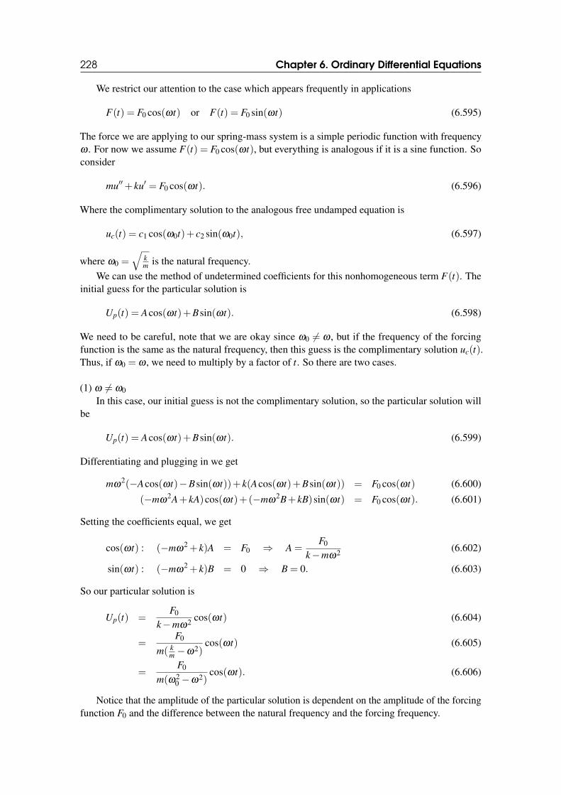
228 Chapter 6. Ordinary Differential Equations
We restrict our attention to the case which appears frequently in applications
F(t) = F0 cos(ωt) or F(t) = F0 sin(ωt) (6.595)
The force we are applying to our spring-mass system is a simple periodic function with frequencyω . For now we assume F(t) = F0 cos(ωt), but everything is analogous if it is a sine function. Soconsider
mu′′+ ku′ = F0 cos(ωt). (6.596)
Where the complimentary solution to the analogous free undamped equation is
uc(t) = c1 cos(ω0t)+ c2 sin(ω0t), (6.597)
where ω0 =√
km is the natural frequency.
We can use the method of undetermined coefficients for this nonhomogeneous term F(t). Theinitial guess for the particular solution is
Up(t) = Acos(ωt)+Bsin(ωt). (6.598)
We need to be careful, note that we are okay since ω0 6= ω , but if the frequency of the forcingfunction is the same as the natural frequency, then this guess is the complimentary solution uc(t).Thus, if ω0 = ω , we need to multiply by a factor of t. So there are two cases.
(1) ω 6= ω0
In this case, our initial guess is not the complimentary solution, so the particular solution willbe
Up(t) = Acos(ωt)+Bsin(ωt). (6.599)
Differentiating and plugging in we get
mω2(−Acos(ωt)−Bsin(ωt))+ k(Acos(ωt)+Bsin(ωt)) = F0 cos(ωt) (6.600)
(−mω2A+ kA)cos(ωt)+(−mω
2B+ kB)sin(ωt) = F0 cos(ωt). (6.601)
Setting the coefficients equal, we get
cos(ωt) : (−mω2 + k)A = F0 ⇒ A =
F0
k−mω2 (6.602)
sin(ωt) : (−mω2 + k)B = 0 ⇒ B = 0. (6.603)
So our particular solution is
Up(t) =F0
k−mω2 cos(ωt) (6.604)
=F0
m( km −ω2)
cos(ωt) (6.605)
=F0
m(ω20 −ω2)
cos(ωt). (6.606)
Notice that the amplitude of the particular solution is dependent on the amplitude of the forcingfunction F0 and the difference between the natural frequency and the forcing frequency.
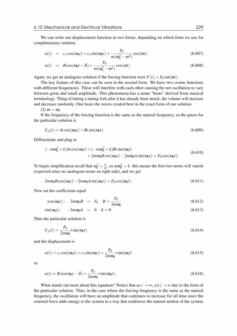
6.10 Mechanical and Electrical Vibrations 229
We can write our displacement function in two forms, depending on which form we use forcomplimentary solution.
u(t) = c1 cos(ω0t)+ c2 sin(ω0t)+F0
m(ω20 −ω2)
cos(ωt) (6.607)
u(t) = Rcos(ω0t−δ )+F0
m(ω20 −ω2)
cos(ωt) (6.608)
Again, we get an analagous solution if the forcing function were F(t) = F0 sin(ωt).The key feature of this case can be seen in the second form. We have two cosine functions
with different frequencies. These will interfere with each other causing the net oscillation to varybetween great and small amplitude. This phenomena has a name "beats" derived from musicalterminology. Thing of hitting a tuning fork after it has already been struck, the volume will increaseand decrease randomly. One hears the waves created here in the exact form of our solution.
(2) ω = ω0If the frequency of the forcing function is the same as the natural frequency, so the guess for
the particular solution is
Up(t) = At cos(ω0t)+Bt sin(ω0t) (6.609)
Differentiate and plug in
(−mω20 + k)At cos(ω0t)+(−mω
20 + k)Bt sin(ω0t)
+2mω0Bcos(ω0t)−2mω0Asin(ω0t) = F0 cos(ω0t).(6.610)
To begin simplification recall that ω20 = k
m , so mω20 = k. this means the first two terms will vanish
(expected since no analogous terms on right side), and we get
2mω0Bcos(ω0t)−2mω0Asin(ω0t) = F0 cos(ω0t). (6.611)
Now set the coefficients equal
cos(ω0t) : 2mω0B = F0 B =F0
2mω0(6.612)
sin(ω0t) : −2mω0A = 0 A = 0 (6.613)
Thus the particular solution is
Up(t) =F0
2mω0t sin(ω0t) (6.614)
and the displacement is
u(t) = c1 cos(ω0t)+ c2 sin(ω0t)+F0
2mω0t sin(ω0t) (6.615)
or
u(t) = Rcos(ω0t−δ )+F0
2mω0t sin(ω0t). (6.616)
What stands out most about this equation? Notice that as t→ ∞, u(t)→ ∞ due to the form ofthe particular solution. Thus, in the case where the forcing frequency is the same as the naturalfrequency, the oscillation will have an amplitude that continues to increase for all time since theexternal force adds energy to the system in a way that reinforces the natural motion of the system.
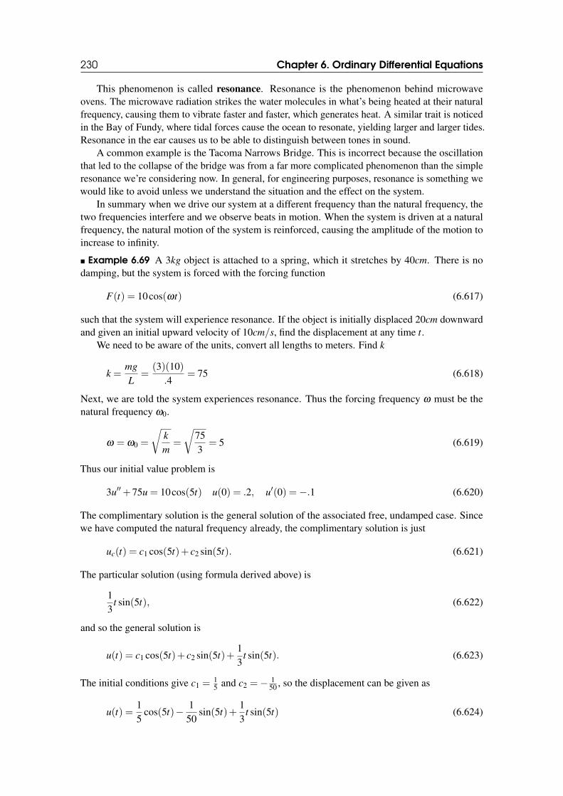
230 Chapter 6. Ordinary Differential Equations
This phenomenon is called resonance. Resonance is the phenomenon behind microwaveovens. The microwave radiation strikes the water molecules in what’s being heated at their naturalfrequency, causing them to vibrate faster and faster, which generates heat. A similar trait is noticedin the Bay of Fundy, where tidal forces cause the ocean to resonate, yielding larger and larger tides.Resonance in the ear causes us to be able to distinguish between tones in sound.
A common example is the Tacoma Narrows Bridge. This is incorrect because the oscillationthat led to the collapse of the bridge was from a far more complicated phenomenon than the simpleresonance we’re considering now. In general, for engineering purposes, resonance is something wewould like to avoid unless we understand the situation and the effect on the system.
In summary when we drive our system at a different frequency than the natural frequency, thetwo frequencies interfere and we observe beats in motion. When the system is driven at a naturalfrequency, the natural motion of the system is reinforced, causing the amplitude of the motion toincrease to infinity.
Example 6.69 A 3kg object is attached to a spring, which it stretches by 40cm. There is nodamping, but the system is forced with the forcing function
F(t) = 10cos(ωt) (6.617)
such that the system will experience resonance. If the object is initially displaced 20cm downwardand given an initial upward velocity of 10cm/s, find the displacement at any time t.
We need to be aware of the units, convert all lengths to meters. Find k
k =mgL
=(3)(10)
.4= 75 (6.618)
Next, we are told the system experiences resonance. Thus the forcing frequency ω must be thenatural frequency ω0.
ω = ω0 =
√km
=
√753
= 5 (6.619)
Thus our initial value problem is
3u′′+75u = 10cos(5t) u(0) = .2, u′(0) =−.1 (6.620)
The complimentary solution is the general solution of the associated free, undamped case. Sincewe have computed the natural frequency already, the complimentary solution is just
uc(t) = c1 cos(5t)+ c2 sin(5t). (6.621)
The particular solution (using formula derived above) is
13
t sin(5t), (6.622)
and so the general solution is
u(t) = c1 cos(5t)+ c2 sin(5t)+13
t sin(5t). (6.623)
The initial conditions give c1 =15 and c2 =− 1
50 , so the displacement can be given as
u(t) =15
cos(5t)− 150
sin(5t)+13
t sin(5t) (6.624)
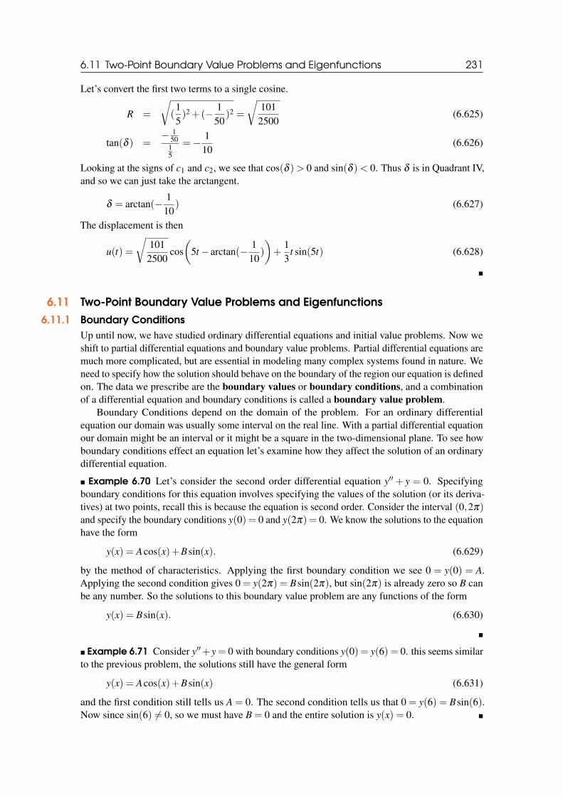
6.11 Two-Point Boundary Value Problems and Eigenfunctions 231
Let’s convert the first two terms to a single cosine.
R =
√(15)2 +(− 1
50)2 =
√1012500
(6.625)
tan(δ ) =− 1
5015
=− 110
(6.626)
Looking at the signs of c1 and c2, we see that cos(δ )> 0 and sin(δ )< 0. Thus δ is in Quadrant IV,and so we can just take the arctangent.
δ = arctan(− 110
) (6.627)
The displacement is then
u(t) =
√1012500
cos(
5t− arctan(− 110
)
)+
13
t sin(5t) (6.628)
6.11 Two-Point Boundary Value Problems and Eigenfunctions6.11.1 Boundary Conditions
Up until now, we have studied ordinary differential equations and initial value problems. Now weshift to partial differential equations and boundary value problems. Partial differential equations aremuch more complicated, but are essential in modeling many complex systems found in nature. Weneed to specify how the solution should behave on the boundary of the region our equation is definedon. The data we prescribe are the boundary values or boundary conditions, and a combinationof a differential equation and boundary conditions is called a boundary value problem.
Boundary Conditions depend on the domain of the problem. For an ordinary differentialequation our domain was usually some interval on the real line. With a partial differential equationour domain might be an interval or it might be a square in the two-dimensional plane. To see howboundary conditions effect an equation let’s examine how they affect the solution of an ordinarydifferential equation.
Example 6.70 Let’s consider the second order differential equation y′′+ y = 0. Specifyingboundary conditions for this equation involves specifying the values of the solution (or its deriva-tives) at two points, recall this is because the equation is second order. Consider the interval (0,2π)and specify the boundary conditions y(0) = 0 and y(2π) = 0. We know the solutions to the equationhave the form
y(x) = Acos(x)+Bsin(x). (6.629)
by the method of characteristics. Applying the first boundary condition we see 0 = y(0) = A.Applying the second condition gives 0 = y(2π) = Bsin(2π), but sin(2π) is already zero so B canbe any number. So the solutions to this boundary value problem are any functions of the form
y(x) = Bsin(x). (6.630)
Example 6.71 Consider y′′+y = 0 with boundary conditions y(0) = y(6) = 0. this seems similarto the previous problem, the solutions still have the general form
y(x) = Acos(x)+Bsin(x) (6.631)
and the first condition still tells us A = 0. The second condition tells us that 0 = y(6) = Bsin(6).Now since sin(6) 6= 0, so we must have B = 0 and the entire solution is y(x) = 0.

232 Chapter 6. Ordinary Differential Equations
Boundary value problems occur in nature all the time. Examine the examples physically. Weknow from previous chapters y′′+ y = 0 models an oscillator such as a rock hanging from a spring.The rock will oscillate with frequency 1
2π. The condition y(0) = 0 just means that when we start
observing, we want the rock to be at the equilibrium spot. If we specify y(2π) = 0, this willautomatically happen, since the motion is 2π periodic. On the other hand, it is impossible for therock to return to the equilibrium point after 6 seconds. It will come back in 2π seconds, which ismore than 6. So the only possible way the rock can be at equilibrium after 6 seconds is if it doesnot leave, which is why the only solution is the zero solution.
The previous examples are homogeneous boundary value problems. We say that a boundaryproblem is homogeneous if the equation is homogeneous and the two boundary conditions involvezero. That is, homogeneous boundary conditions might be one of these types
y(x1) = 0 y(x2) = 0 (6.632)
y′(x1) = 0 y(x2) = 0 (6.633)
y(x1) = 0 y′(x2) = 0 (6.634)
y′(x1) = 0 y′(x2) = 0. (6.635)
On the other hand, if the equation is nonhomogeneous or any of the boundary conditions do notequal zero, then the boundary value problem is nonhomogenous or inhomogeneous. Let’s look atsome examples of nonhomogeneous boundary value problems.
Example 6.72 Take y′′+9y = 0 with boundary conditions y(0) = 2 and y(π
6 ) = 1. The generalsolution to the differential equation is
y(x) = Acos(3x)+Bsin(3x). (6.636)
The two conditions give
2 = y(0) = A (6.637)
1 = y(π
6) = B (6.638)
so that the solution is
y(x) = 2cos(3x)+ sin(3x) (6.639)
Example 6.73 Take y′′+9y = 0 with boundary conditions y(0) = 2 and y(2π) = 2. The generalsolution to the differential equation is
y(x) = Acos(3x)+Bsin(3x). (6.640)
The two conditions give
2 = y(0) = A (6.641)
2 = y(2π) = A. (6.642)
This time the second condition did not give and new information, like in Example 1 and B does notaffect whether or not the solution satisfies the boundary conditions or not. We then have infinitelymany solutions of the form
y(x) = 2cos(3x)+Bsin(3x) (6.643)

6.11 Two-Point Boundary Value Problems and Eigenfunctions 233
Example 6.74 Take y′′+9y = 0 with boundary conditions y(0) = 2 and y(2π) = 4. The generalsolution to the differential equation is
y(x) = Acos(3x)+Bsin(3x). (6.644)
The two conditions give
2 = y(0) = A (6.645)
4 = y(2π) = A. (6.646)
On one hand, A = 2 and by the second equation A = 4. This is impossible and this boundary valueproblem has no solutions.
These examples illustrate that a small change to the boundary conditions can dramaticallychange the problem, unlike small changes in the initial data for initial value problems.
6.11.2 Eigenvalue ProblemsRecall the system studied extensively in previous chapters
Ax = λx (6.647)
where for certain values of λ , called eigenvalues, there are nonzero solutions called eigenvectors.We have a similar situation with boundary value problems.
Consider the problem
y′′+λy = 0 (6.648)
with boundary conditions y(0) = 0 and y(π) = 0. The values of λ where we get nontrivial (nonzero)solutions will be eigenvalues. The nontrivial solutions themselves are called eigenfunctions.
We need to consider three cases separately.(1) If λ > 0, then it is convenient to let λ = µ2 and rewrite the equation as
y′′+µ2y = 0 (6.649)
The characteristic polynomial is r2 +µ2 = 0 with roots r =±iµ . So the general solution is
y(x) = Acos(µx)+Bsin(µx) (6.650)
Note that µ 6= 0 since λ > 0. Recall the boundary conditions are y(0) = 0 and y(π) = 0. So thefirst boundary condition gives A = 0. The second boundary condition reduces to
Bsin(µπ) = 0 (6.651)
For nontrivial solutions B 6= 0. So sin(µπ) = 0. Thus µ = 1,2,3, ... and thus the eigenvalues λn
are 1,4,9, ...,n2. The eigenfunctions are only determined up to arbitrary constant, so convention isto choose the arbitrary constant to be 1. Thus the eigenfunctions are
y1(x) = sin(x) y2(x) = sin(2x), ...,yn(x) = sin(nx) (6.652)
(2) If λ < 0, let λ =−µ2. So the above equation becomes
y′′−µ2y = 0 (6.653)
234 Chapter 6. Ordinary Differential Equations
The characteristic equation is r2−µ2 = 0 with roots r =±µ , so its general solution can be writtenas
y(x) = Acosh(µx)+Bsinh(µx) =Ceµx +De−µx (6.654)
The first boundary condition, if considering the first form, gives A = 0. The second boundarycondition gives Bsinh(µπ) = 0. Since µ 6= 0, then sinh(µπ) 6= 0, and therefore B = 0. So forλ < 0 the only solution is y = 0, there are no nontrivial solutions and thus no eigenvalues.
(3) If λ = 0, then the equation above becomes
y′′ = 0 (6.655)
and the general solution if we integrate twice is
y(x) = Ax+B (6.656)
The boundary conditions are only satisfied when A = 0 and B = 0. So there is only the trivialsolution y = 0 and λ = 0 is not an eigenvalue.
To summarize we only get real eigenvalues and eigenvectors when λ > 0. There may becomplex eigenvalues. A basic problem studied later in the chapter is
y′′+λy = 0, y(0) = 0, y(L) = 0 (6.657)
Hence the eigenvalues and eigenvectors are
λn =n2π2
L2 , yn(x) = sin(nπx
L) for n = 1,2,3, ... (6.658)
This is the classical Euler Buckling Problem.Review Euler’s Equations:
Example 6.75 Consider equation of the form
t2y′′+ ty′+ y = 0 (6.659)
and let x = ln(t). Then
dydt
=dydx
dxdt
=1t
dydx
(6.660)
d2ydx2 =
ddt(dydx
)1t+
dydx
(1t)dydx
(6.661)
=d2ydx2
1t2 +
dydx
(− 1t2 ) (6.662)
(6.663)
Plug these back into the original equation
t2y′′+ ty+ y =d2ydx2 −
dydx
+dydx
+ y = 0 (6.664)
= y′′+ y = 0 (6.665)
Thus the characteristic equation is r2 +1 = 0, which has roots r =±i. So the general solution is
y(x) = c1 cos(x)+ c2 sin(x) (6.666)
Recalling that x = ln(t) our final solution is
y(x) = c1 cos(ln(t))+ c2 sin(ln(t)) (6.667)

6.12 Systems of Differential Equations 235
6.12 Systems of Differential Equations
To this point we have focused on solving a single equation, but may real world systems are given asa system of differential equations. An example is Population Dynamics, Normally the death rate ofa species is not a constant but depends on the population of predators. An example of a system offirst order linear equations is
x′1 = 3x1 + x2 (6.668)
x′2 = 2x1−4x2 (6.669)
We call a system like this coupled because we need to know what x1 is to know what x2 is and viceversa. It is important to note that there will be a lot of similarities between our discussion and theprevious sections on second and higher order linear equations. This is because any higher orderlinear equation can be written as a system of first order linear differential equations.
Example 6.76 Write the following second order differential equation as a system of first orderlinear differential equations
y′′+4y′− y = 0, y(0) = 2, y′(0) =−2 (6.670)
All that is required to rewrite this equation as a first order system is a very simple change ofvariables. In fact, this is ALWAYS the change of variables to use for a problem like this. We set
x1(t) = y(t) (6.671)
x2(t) = y′(t) (6.672)
Then we have
x′1 = y′ = x2 (6.673)
x′2 = y′′ = y−4y′ = x1−4x2 (6.674)
Notice how we used the original differential equation to obtain the second equation. The firstequation, x′1 = x2, is always something you should expect to see when doing this. All we have leftto do is to convert the initial conditions.
x1(0) = y(0) = 2 (6.675)
x2(0) = y′(0) =−2 (6.676)
Thus our original initial value problem has been transformed into the system
x′1 = x2, x1(0) = 2 (6.677)
x′2 = x1−4x2, x2(0) =−2 (6.678)
Let’s do an example for higher order linear equations.
Example 6.77
y(4)+ ty′′′−2y′′−3y′− y = 0 (6.679)
as a system of first order differential equations.

236 Chapter 6. Ordinary Differential Equations
We want to use a similar change of variables as the previous example. The only difference isthat since our equation in this example is fourth order we will need four new variables instead oftwo.
x1 = y (6.680)
x2 = y′ (6.681)
x3 = y′′ (6.682)
x4 = y′′′ (6.683)
Then we have
x′1 = y′ = x2 (6.684)
x′2 = y′′ = x3 (6.685)
x′3 = y′′′ = x4 (6.686)
x′4 = y(4) = y+3y′+2y′′− ty′′′ = x1 +3x2 +2x3− tx4 (6.687)
as our system of equations. To be able to solve these, we need to review some facts about systemsof equations and linear algebra.
6.13 Homogeneous Linear Systems with Constant CoefficientsA two-dimensional equation has the form
x′ = ax+by (6.688)
y′ = cx+dy (6.689)
Suppose we have got our system written in matrix form
x′ = Ax (6.690)
How do we solve this equation? If A were a 1×1 matrix, i.e. a constant, and x were a vector with 1component, the differential equation would be the separable equation
x′ = ax (6.691)
We know this is solved by
x(t) = ceat . (6.692)
One might guess, then, that in the n× n case, instead of a we have some other constant in theexponential, and instead of the constant of integration c we have some constant vector η . So ourguess for the solution will be
x(t) = ηert . (6.693)
Plugging the guess into the differential equation gives
rηert = Aηert (6.694)
(Aη− rη)ert = 0 (6.695)
(A− rI)ηert = 0. (6.696)
Since ert 6= 0, we end up with the requirement that
(A− rI)η = 0 (6.697)

6.13 Homogeneous Linear Systems with Constant Coefficients 237
This should seem familiar, it is the condition for η to be an eigenvector of A with eigenvalue r.Thus, we conclude that for (6.693) to be a solution of the original differential equation, we musthave η an eigenvalue of A with eigenvalue r.
That tells us how to get some solutions to systems of differential equations, we find theeigenvalues and vectors of the coefficient matrix A, then form solutions using (6.693). But howwill we form the general solution?
Thinking back to the second/higher order linear case, we need enough linearly independentsolutions to form a fundamental set. As we noticed last lecture, if we have all simple eigenvalues,then all the eigenvectors are linearly independent, and so the solutions formed will be as well. Wewill handle the case of repeated eigenvalues later.
So we will find the fundamental solutions of the form (6.693), then take their linear combina-tions to get our general solution.
6.13.1 The Phase Plane
We are going to rely on qualitatively understanding what solutions to a linear system of differentialequations look like, this will be important when considering nonlinear equations. We know thetrivial solution x = 0 is always a solution to our homogeneous system x′ = Ax. x = 0 is an exampleof an equilibrium solution, i.e. it satisfies
x′ = Ax = 0 (6.698)
and is a constant solution. We will assume our coefficient matrix A is nonsingular (det(A) 6= 0),thus x = 0 is the only equilibrium solution.
The question we want to ask is whether other solutions move towards or away from this constantsolution as t→±∞, so that we can understand the long term behavior of the system. This is nodifferent than what we did when we classified equilibrium solutions for first order autonomousequations, we will generalize the ideas to systems of equations.
When we drew solution spaces then, we did so on the ty-plane. To do something analogous wewould require three dimensions, since we would have to sketch both x1 and x2 vs. t. Instead, whatwe do is ignore t and think of our solutions as trajectories on the x1x2-plane. Then our equilibriumsolution is the origin. The x1x2-plane is called the phase plane. We will see examples where wesketch solutions, called phase portraits.
6.13.2 Real, Distinct Eigenvalues
Lets get back to the equation x′ = Ax. We know if λ1 and λ2 are real and distinct eigenvalues of the2×2 coefficient matrix A associated with eigenvectors η(1) and η(2), respectively. We know fromabove η(1) and η(2) are linearly independent, as λ1 and λ2 are simple. Thus the solutions obtainedfrom them using (6.693) will also be linearly independent, and in fact will form a fundamental setof solutions. The general solution is
x(t) = c1eλ1tη(1)+ c2eλ2t
η(2) (6.699)
So if we have real, distinct eigenvalues, all that we have to do is find the eigenvectors, form thegeneral solution as above, and use any initial conditions that may exist.
Example 6.78 Solve the following initial value problem
x′ =(−2 22 1
)x x(0) =
(50
)(6.700)

238 Chapter 6. Ordinary Differential Equations
The first thing we need to do is to find the eigenvalues of the coefficient matrix.
0 = det(A−λ I) =
∣∣∣∣ −2−λ 22 1−λ
∣∣∣∣ (6.701)
= λ2 +λ −6 (6.702)
= (λ −2)(λ +3) (6.703)
So the eigenvalues are λ1 = 2 and λ2 =−3. Next we need the eigenvectors.
(1) λ1 = 2
(A−2I)η = 0 (6.704)(−4 22 −1
)(η1η2
)=
(00
)(6.705)
So we will want to find solutions to the system
−4η1 +2η2 = 0 (6.706)
2η1−η2 = 0. (6.707)
Using either equation we find η2 = 2η1, and so any eigenvector has the form
η =
(η1η2
)=
(η12η1
)(6.708)
Choosing η1 = 1 we obtain the first eigenvector
η(1) =
(12
). (6.709)
(2) λ2 =−3
(A+3I)η = 0 (6.710)(1 22 4
)(η1η2
)=
(00
)(6.711)
So we will want to find solutions to the system
η1 +2η2 = 0 (6.712)
2η1 +4η2 = 0. (6.713)
Using either equation we find η1 =−2η2, and so any eigenvector has the form
η =
(η1η2
)=
(−2η2
η2
). (6.714)
Choosing η2 = 1 we obtain the second eigenvector
η(2) =
(−21
). (6.715)
6.13 Homogeneous Linear Systems with Constant Coefficients 239
Thus our general solution is
x(t) = c1e2t(
12
)+ c2e−3t
(−21
). (6.716)
Now let’s use the initial condition to solve for c1 and c2. The condition says(50
)= x(0) = c1
(12
)+ c2
(−21
). (6.717)
All that’s left is to write out is the matrix equation as a system of equations and then solve.
c1−2c2 = 5 (6.718)
2c1 + c2 = 0 ⇒ c1 = 1,c2 =−2 (6.719)
Thus the particular solution is
x(t) = e2t(
12
)−2e−3t
(−21
). (6.720)
Example 6.79 Sketch the phase portrait of the system from Example 1.In the last example we saw that the eigenvalue/eigenvector pairs for the coefficient matrix were
λ1 = 2 η(1) =
(12
)(6.721)
λ2 = −3 η(2) =
(−21
). (6.722)
The starting point for the phase portrait involves sketching solutions corresponding to the eigenvec-tors (i.e. with c1 or c2 = 0). We know that if x(t) is one of these solutions
x′(t) = Acieλitη(i) = ciλieλitη(i). (6.723)
This is just, for any t, a constant times the eigenvector, which indicates that lines in the direction ofthe eigenvector are these solutions to the system. There are called eigensolutions of the system.
Next, we need to consider the direction that these solutions move in. Let’s start with the firsteigensolution, which corresponds to the solution with c2 = 0. The first eigenvalue is λ1 = 2 > 0.This indicates that this eigensolution will grow exponentially, as the exponential in the solution hasa positive exponent. The second eigensolution corresponds to λ2 =−3 < 0, so the exponential inthe appropriate solution is negative. Hence this solution will decay and move towards the origin.
What does the typical trajectory do (i.e. a trajectory where both c1,c2 6= 0)? The generalsolution is
x(t) = c1e2tη(1)+ c2e−3t
η(2). (6.724)
Thus as t→ ∞, this solution will approach the positive eigensolution, as the component correspond-ing to the negative eigensolution will decay away. On the other hand, as t →−∞, the trajectorywill asymptotically reach the negative eigensolution, as the positive eigensolution component willbe tiny. The end result is the phase portrait as in Figure 1. When the phase portrait looks like this(which happens in all cases with eigenvalues of mixed signs), the equilibrium solution at the originis classified as a saddle point and is unstable.

240 Chapter 6. Ordinary Differential Equations
Figure 6.4: Phase Portrait of the saddle point in Example 1
Example 6.80 Solve the following initial value problem.
x′1 = 4x1 + x2 x1(0) = 6 (6.725)
x′2 = 3x1 +2x2 x2(0) = 2 (6.726)
Before we can solve anything, we need to convert this system into matrix form. Doing so convertsthe initial value problem to
x′ =(
4 13 2
)x x(0) =
(62
). (6.727)
To solve, the first thing we need to do is to find the eigenvalues of the coefficient matrix.
0 = det(A−λ I) =
∣∣∣∣ 4−λ 13 2−λ
∣∣∣∣ (6.728)
= λ2−6λ +5 (6.729)
= (λ −1)(λ −5) (6.730)
So the eigenvalues are λ1 = 1 and λ2 = 5. Next, we find the eigenvectors.(1) λ1 = 1
(A− I)η = 0 (6.731)(3 13 1
)(η1η2
)=
(00
)(6.732)
So we will want to find solutions to the system
3η1 +η2 = 0 (6.733)
3η1 +η2 = 0. (6.734)
Using either equation we find η2 =−3η1, and so any eigenvector has the form
η =
(η1η2
)=
(η1−3η1
)(6.735)
6.13 Homogeneous Linear Systems with Constant Coefficients 241
Choosing η1 = 1 we obtain the first eigenvector
η(1) =
(1−3
). (6.736)
(2) λ2 = 5
(A−5I)η = 0 (6.737)(−1 13 −3
)(η1η2
)=
(00
)(6.738)
So we will want to find solutions to the system
−η1 +η2 = 0 (6.739)
3η1−3η2 = 0. (6.740)
Using either equation we find η1 = η2, and so any eigenvector has the form
η =
(η1η2
)=
(η2η2
). (6.741)
Choosing η2 = 1 we obtain the second eigenvector
η(2) =
(11
). (6.742)
Thus our general solution is
x(t) = c1et(
1−3
)+ c2e5t
(11
). (6.743)
Now using our initial conditions we solve for c1 and c2. The condition gives(62
)= x(0) = c1
(1−3
)+ c2
(11
). (6.744)
All that is left is to write out this matrix equation as a system of equations and then solve
c1 + c2 = 6 (6.745)
−3c1 + c2 = 2⇒ c1 = 1,c2 = 5 (6.746)
Thus the particular solution is
x(t) = et(
1−3
)+5e5t
(11
). (6.747)
Example 6.81 Sketch the phase portrait of the system from Example 3.In the last example, we saw that the eigenvalue/eigenvector pairs for the coefficient matrix were
λ1 = 1 η(1) =
(1−3
). (6.748)
λ2 = 5 η(2) =
(11
). (6.749)

242 Chapter 6. Ordinary Differential Equations
Figure 6.5: Phase Portrait of the unstable node in Example 2
We begin by sketching the eigensolutions (these are straight lines in the directions of the eigenvec-tors). Both of these trajectories move away from the origin, though, as the eigenvalues are bothpositive.
Since |λ2| > |λ1|, we call the second eigensolution the fast eigensolution and the first onethe slow eigensolution. The term comes from the fact that the eigensolution corresponds to theeigenvalue with larger magnitude will either grow or decay more quickly than the other one.
As both grow in forward time, asymptotically, as t→ ∞, the fast eigensolution will dominatethe typical trajectory, as it gets larger much more quickly than the slow eigensolution does. So inforward time, other trajectories will get closer and closer to the eigensolution corresponding to η(2).On the other hand, as t→−∞, the fast eigensolution will decay more quickly than the slow one,and so the eigensolution corresponding to η(1) will dominate in backwards time.
Thus the phase portrait will look like Figure 2. Whenever we have two positive eigenvalues,every solution moves away from the origin. We call the equilibrium solution at the origin, in thiscase, a node and classify it as being unstable.
Example 6.82 Solve the following initial value problem.
x′1 = −5x1 + x2 x1(0) = 2 (6.750)
x′2 = 2x1−4x2 x2(0) =−1 (6.751)
We convert this system into matrix form.
x′ =(−5 12 −4
)x x(0) =
(2−1
). (6.752)
To solve, the first thing we need to do is to find the eigenvalues of the coefficient matrix.
0 = det(A−λ I) =
∣∣∣∣ −5−λ 12 −4−λ
∣∣∣∣ (6.753)
= λ2 +9λ +18 (6.754)
= (λ +3)(λ +6) (6.755)

6.13 Homogeneous Linear Systems with Constant Coefficients 243
So the eigenvalues are λ1 =−3 and λ2 =−6. Next, we find the eigenvectors.(1) λ1 =−3
(A+3I)η = 0 (6.756)(−2 12 −1
)(η1η2
)=
(00
)(6.757)
So we will want to find solutions to the system
−2η1 +η2 = 0 (6.758)
2η1−η2 = 0. (6.759)
Using either equation we find η2 = 2η1, and so any eigenvector has the form
η =
(η1η2
)=
(η1
2η1
)(6.760)
Choosing η1 = 1 we obtain the first eigenvector
η(1) =
(12
). (6.761)
(2) λ2 =−6
(A+6I)η = 0 (6.762)(1 12 2
)(η1η2
)=
(00
)(6.763)
So we will want to find solutions to the system
η1 +η2 = 0 (6.764)
2η1 +2η2 = 0. (6.765)
Using either equation we find η1 =−η2, and so any eigenvector has the form
η =
(η1η2
)=
(−η2η2
). (6.766)
Choosing η2 = 1 we obtain the second eigenvector
η(2) =
(−11
). (6.767)
Thus our general solution is
x(t) = c1e−3t(
12
)+ c2e−6t
(−11
). (6.768)
Now using our initial conditions we solve for c1 and c2. The condition gives(2−1
)= x(0) = c1
(12
)+ c2
(−11
). (6.769)

244 Chapter 6. Ordinary Differential Equations
Figure 6.6: Phase Portrait of the Stable Node in Example 3
All that is left is to write out this matrix equation as a system of equations and then solve
c1− c2 = 2 (6.770)
2c1 + c2 = −1⇒ c1 =13,c2 =−
53
(6.771)
Thus the particular solution is
x(t) =13
e−3t(
12
)− 5
3e−6t
(−11
). (6.772)
Example 6.83 Sketch the phase portrait of the system from Example 5.In the last example, we saw that the eigenvalue/eigenvector pairs for the coefficient matrix were
λ1 = −3 η(1) =
(12
)(6.773)
λ2 = −6 η(2) =
(−11
). (6.774)
We begin by sketching the eigensolutions. Both of these trajectories decay towards the ori-gin, since both eigenvalues are negative. Since |λ2| > |λ1|, the second eigensolution is the fasteigensolution and the first one the slow eigensolution. In the general solution, both exponentialsare negative and so every solution will decay and move towards the origin. Asymptotically, ast→ ∞ the trajectory gets closer and closer to the origin, the slow eigensolution will dominate thetypical trajectory, as it dies out less quickly than the fast eigensolution. So in forward time, othertrajectories will get closer and closer to the eigensolution corresponding to η(1). On the other hand,as t→−∞, the fast solution will grow more quickly than the slow one, and so the eigensolutioncorresponding to η(2) will dominate in backwards time.
Thus the phase portrait will look like Figure 3. Whenever we have two negative eigenvalues,every solution moves toward the origin. We call the equilibrium solution at the origin, in this case,a node and classify it as being asymptotically stable.

V7 Fourier Series and Transforms . . . . . . . . 2477.1 Introduction to Fourier Series7.2 Fourier Coefficients7.3 Fourier Coefficients7.4 Dirichlet Conditions7.5 Convergence and Sum of a Fourier series7.6 Complex Form of Fourier Series7.7 Complex Fourier Series7.8 General Fourier Series for Functions of Any Period
p = 2L7.9 Even and Odd Functions7.10 Even and Odd Functions, Half-Range Expansions
8 Partial Differential Equations . . . . . . . . . 2758.1 Introduction to Basic Classes of PDEs8.2 Introduction to PDEs8.3 Laplace’s Equations and Steady State Temperature
Problems8.4 Heat Equation and Schrödinger Equation8.5 Separation of Variables and Heat Equation IVPs8.6 Heat Equation Problems8.7 Other Boundary Conditions8.8 The Schrödinger Equation8.9 Wave Equations and the Vibrating String
Index . . . . . . . . . . . . . . . . . . . . . . . . . . . . . . 303
Part Five: PDEs and FourierSeries


7. Fourier Series and Transforms
7.1 Introduction to Fourier SeriesFourier series have many applications in the physical sciences. For example, in vibrations andoscillations→ Think Frequency! The key idea behind Fourier series is to provide an alternativeway of expressing a function to the traditional power series, f (x) = ∑
∞n=0
f (n)(0)xn
n! . Instead let usexpress a function as a sum of sines and cosines
f (x) =∞
∑m=0
[an cos(mπx)+bn sin(mπx)] . (7.1)
This does remarkably well at approximating functions. Notice though that the resulting function isperiodic. Fourier series are also a key tool in solving PDEs (more later).
7.1.1 Simple Harmonic MotionImagine a particle at point p moves around the circle at a constant speed. Let the mass be theprojection of p onto a vertical line (spring-mass system). Also, let ω be the angular velocity of p.Thus, θ = ωt and the position of the mass is c = sin(θ) = ωt. The motion of the point c traces outa sine curve and this motion is called Simple Harmonic Motion.
Definition 7.1.1 (Simple Harmonic Motion) Simple harmonic motion can take the forms:
sin(ωt), cos(ωt), sin(ωt +φ), (7.2)
where ω is the angular velocity and φ is the phase (horizontal displacement). Traditionalexamples include a hanging mass from a spring a pendulum, and a tuning fork.
The location of the point p = (Acos(ωt),Asin(ωt)) = Aeiωt if P = x + iy. Here A is theamplitude or the maximum displacement of the object. We also can write down the equation for themotion of the point c
dydt
=ddt
(Asin(ωt)) = Aω cos(ωt) = Bcos(ωt),

248 Chapter 7. Fourier Series and Transforms
Figure 7.1: Convergence of Fourier Series to a step function (square wave). K is the number ofterms.
a)
b)
Figure 7.2: Depiction of simple harmonic motion using a point rotating around the unit circle or aspring mass system.
where B = Aω is the maximum velocity achieved by the object. In physics we can define the kineticenergy:
KE =12
mv2 =12
m(
dydt
)2
=12
mB2 cos2(ωt)≤ 12
mB2.
Therefore, the maximum energy of the system, 12 mB2, is proportional to the maximum velocity B
(and therefore the amplitude A).Since sine/cosine are periodic, one we know the value on the interval [0,2π) (or [0,L)), then
we know the value everywhere.

7.2 Fourier Coefficients 249
Example 7.1 Consider the general function representing simple harmonic motion
y(x, t) := Acos[2π
( xλ− f t
)]= Acos
[2π
λ(x− vt)
]. (7.3)
Here A is the amplitude, λ is the wavelength, f = ω
2πis the frequency, T = 1
f =2π
ωis the period,
and v = f λ is the velocity.
From an ODE perspective (think last chapter) we have an equation for simple harmonic motion:
Fnet = md2xdt2 =−kx (Hooke’s Law) ⇒ x′′+
km
x = 0. (7.4)
Solving this equation with the characteristic polynomial gives r2 + km = 0, which implies that
r =√
km i. Thus, the general solution is
x(t) =C1 cos(ωt)+C2 sin(ωt) = Acos(ωt−φ), (7.5)
where angular velocity ω =√
km , the amplitude A =
√C2
1 +C22 (depends on initial/boundary
conditions), and the phase φ = tan−1(
C2C1
). The frequency f = ω
2π= 1
2π
√km and the period
T = 1f = 2π
√mk .
Many common periodic functions are not continuous or differentiable such as the square wave,the sawtooth, or the rectified half wave (semi-circle wave). Problem: Given a function f (x) howan we expand it into a series of sines and cosines.
7.2 Fourier Coefficients
7.3 Fourier CoefficientsThis section follows the outline and layout of Kreyzig Chapter 11. Recall that Fourier series are in-finite series designed to represent general periodic functions in terms of simpler ones (sines/cosines).The immense theory behind Fourier series can seem complicated, but the application of Fourierseries to real problems is much simpler. Fourier series have a distinct advantage over Taylor seriesin that even discontinuous functions have a Fourier series representation while they do not possessa Taylor series.
The main use of Fourier series are in representing periodic functions.
Definition 7.3.1 (Periodic Functions) A function f (x) is called a periodic function if f (x) isdefined for all real x and if there is some positive number p called the period of f (x), such that
f (x+ p) = f (x) (7.6)
for all x. The graph of such a function is obtained from periodic repetition of its graph over anyinterval of length p.
Examples of periodic functions are f (x) = sin(x),cos(x) and examples that are not periodic aref (x) = xn,ex,cosh(x), ln(x).
R If f (x) has a period p, then it also has a period of 2p (and np for any integer n > 0). Since
f (x+2p) = f ([x+ p]+ p) = f (x+ p) = f (x), ⇒ f (x+np) = f (x).
Furthermore, if functions f (x) and g(x) have period p, then a f (x)+bg(x) with any constantsa and b also has period p.

250 Chapter 7. Fourier Series and Transforms
Figure 7.3: Periodic Function. Image from Kreyzig Adv. Engineering Math
Problem: We want to find a representation of a 2π-periodic function in terms of simplefunctions
1,cos(x),sin(x),cos(2x),sin(2x), ...,cos(nx),sin(nx), ..., (7.7)
which are all 2π-periodic (see Figure!7.4). The associated series made up of these terms is called atrigonometric series and has the form
a0+a1 cos(x)+b1 sin(x)+a2 cos(2x)+b2 sin(2x)+ ...= a0+∞
∑n=1
[an cos(nx)+bn sin(nx)] . (7.8)
where a0,a1,b1,a2,b2, ... are all constants called the coefficients of the series. Since each termhas a period of 2π , then if the series converges the result must also have a period of 2π! Given afunction f (x) of period 2π and such that it can be represented by a series of this form, that seriesconverges, and has the sum f (x), then we can use equality to write
f (x) = a0 +∞
∑n=1
[an cos(nx)+bn sin(nx)] . (7.9)
Thus the righthand side is called the Fourier series of f (x).
Figure 7.4: Periodic Trig Function. Image from Kreyzig Adv. Engineering Math
Question: How do we find the coefficients ai,bi for i = 0, ...,n?
Solution: These constants are the so-called Fourier coefficients of f (x), given by Euler for-mulas

7.3 Fourier Coefficients 251
Theorem 7.3.1 (Euler Formulas for Fourier Coefficients)
a0 =1
2π
∫π
−π
f (x)dx
an =1π
∫π
−π
f (x)cos(nx)dx n = 1,2, ...
bn =1π
∫π
−π
f (x)sin(nx)dx n = 1,2, ...
R The Fourier coefficient a0 is actually the average value of the function over its period! In otherwords, if we only take the first term in the Fourier series the function f (x) is approximated byits average value over its period. We can think of this as a “First Approximation".
7.3.1 A Basic Example
Start by considering some basic questions when it comes to Fourier series:1. How are continuous functions able to represent a given discontinuous function?2. How does the quality of the approximation increase as one takes more and more terms in theFourier series?
Example 7.2 (Periodic Rectangular Wave) Find the Fourier coefficients of the periodic function
f (x) =
−k if −π < x < 0k if 0 < x < π
.
This is a typical function representing an external force acting on a mechanical system or electriccircuit (see Fig. 7.5).
Figure 7.5: Square wave periodic function. Image from Kreyzig Adv. Engineering Math

252 Chapter 7. Fourier Series and Transforms
Solution: Start by using the formulas for the Fourier coefficients:
a0 =1
2π
∫π
−π
f (x)dx =1
2π
∫ 0
−π
−kdx+1
2π
∫π
0kdx
=1
2π
[−kx
∣∣∣∣0−π
+ kx∣∣∣∣π0
]=
12π
[−kπ + kπ] = 0
an =1π
∫π
−π
f (x)cos(nx)dx =1π
∫ 0
−π
−k cos(nx)dx+1π
∫π
0k cos(nx)dx
=1π
[−k
nsin(nx)
∣∣∣∣0−π
+kn
sin(nx)∣∣∣∣π0
]=
1π[0+0] = 0
bn =1π
∫π
−π
f (x)sin(nx)dx =1π
∫ 0
−π
−k sin(nx)dx+1π
∫π
0k sin(nx)dx
=1π
[kn
cos(nx)∣∣∣∣0−π
− kn
cos(nx)∣∣∣∣π0
]=
knπ
[1− cos(−nπ)− cos(nπ)+1] =2knπ
(1− cos(nπ)).
Hence, the Fourier sine coefficients are b2n = 0 and b2n+1 =4k
(2n+1)π . Thus, the Fourier series is
f (x) = a0 +∞
∑n=1
[an cos(nx)+bn sin(nx)] =4kπ
(sin(x)+
13
sin(3x)+15
sin(5x)+ . . .
).
A picture depicting the approximation with the partial sums is shown in Fig. 7.6.
7.3.2 Derivation of Euler Formulas
In order to derive the formulas for the Fourier coefficients we heavily rely on the following resultabout the orthogonality of trigonometric functions.
Theorem 7.3.2 (Orthogonality of Trigonometric Functions) On the interval (−π ≤ x≤ π) thefollowing relations hold:∫
π
−π
cos(nx)cos(mx)dx = 0 (n 6= m) (7.10)∫π
−π
sin(nx)sin(mx)dx = 0 (n 6= m) (7.11)∫π
−π
sin(nx)cos(mx)dx = 0 (n 6= m or n = m). (7.12)
This is proved by transforming each product into a single trig function using the sum/differenceformulas.
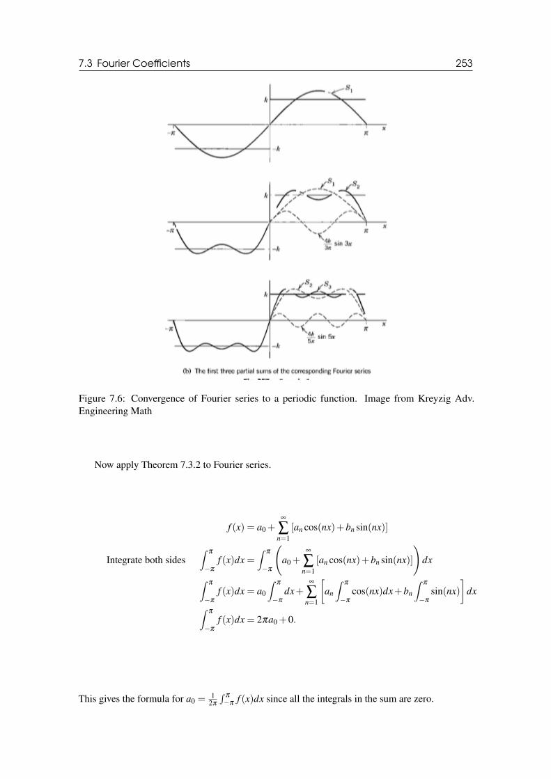
7.3 Fourier Coefficients 253
Figure 7.6: Convergence of Fourier series to a periodic function. Image from Kreyzig Adv.Engineering Math
Now apply Theorem 7.3.2 to Fourier series.
f (x) = a0 +∞
∑n=1
[an cos(nx)+bn sin(nx)]
Integrate both sides∫
π
−π
f (x)dx =∫
π
−π
(a0 +
∞
∑n=1
[an cos(nx)+bn sin(nx)]
)dx
∫π
−π
f (x)dx = a0
∫π
−π
dx+∞
∑n=1
[an
∫π
−π
cos(nx)dx+bn
∫π
−π
sin(nx)]
dx∫π
−π
f (x)dx = 2πa0 +0.
This gives the formula for a0 =1
2π
∫π
−πf (x)dx since all the integrals in the sum are zero.

254 Chapter 7. Fourier Series and Transforms
Now to get the formula for an we repeat this process, but multiply both sides of the expressionfor a Fourier series by cos(mx) before integrating.
f (x) = a0 +∞
∑n=1
[an cos(nx)+bn sin(nx)]
∫π
−π
f (x)cos(mx)dx =∫
π
−π
(a0 +
∞
∑n=1
[an cos(nx)+bn sin(nx)]
)cos(mx)dx
∫π
−π
f (x)cos(mx)dx = a0
∫π
−π
cos(mx)dx+∞
∑n=1
[an
∫π
−π
cos(nx)cos(mx)dx+bn
∫π
−π
sin(nx)cos(mx)]
dx∫π
−π
f (x)cos(nx)dx = an
∫π
−π
cos2(nx)dx = anπ.
This gives the formula for an =1π
∫π
−πf (x)cos(nx)dx.
Now to get the formula for bn we repeat this process, but multiply both sides of the expressionfor a Fourier series by sin(mx) before integrating.
f (x) = a0 +∞
∑n=1
[an cos(nx)+bn sin(nx)]
∫π
−π
f (x)sin(mx)dx =∫
π
−π
(a0 +
∞
∑n=1
[an cos(nx)+bn sin(nx)]
)sin(mx)dx
∫π
−π
f (x)sin(mx)dx = a0
∫π
−π
sin(mx)dx+∞
∑n=1
[an
∫π
−π
cos(nx)sin(mx)dx+bn
∫π
−π
sin(nx)sin(mx)]
dx∫π
−π
f (x)sin(nx)dx = bn
∫π
−π
sin2(nx)dx = bnπ.
This gives the formula for bn =1π
∫π
−πf (x)sin(nx)dx.
Example 7.3 The fundamental period is the smallest positive period. Find it for: cos(x),cos(2x),sin(πx),sin(2πx).
Solution: For cos(x) we know the period is 2π . To find the fundamental period for cos(kx)we need to find when kx = 2π or x = 2π
k . So the fundamental period for cos(2x) is 2π
k = π . Thefundamental period for cos(πx) is 2π
π= 2 and for cos(2πx) is 2π
2π= 1.
Example 7.4 Sketch three periods of the 2π-periodic function defined on the interval−π ≤ x≤ π
as
a) f (x) = x, b) f (x) = π−|x|, c)
1 −π < x < 0cos(1
2 x) 0 < x < π.
Example 7.5 Find the Fourier coefficients of the periodic function
f (x) =
0 if −π < x < 01 if 0 < x < π
.

7.4 Dirichlet Conditions 255
Solution: Start by using the formulas for the Fourier coefficients:
a0 =1
2π
∫π
−π
f (x)dx =1
2π
∫ 0
−π
0dx+1
2π
∫π
01dx
=1
2π
[x∣∣∣∣π0
]=
12π
[π] =12
an =1π
∫π
−π
f (x)cos(nx)dx =1π
∫ 0
−π
0dx+1π
∫π
0cos(nx)dx
=1π
[1n
sin(nx)∣∣∣∣π0
]=
1π[0+0] = 0
bn =1π
∫π
−π
f (x)sin(nx)dx =1π
∫ 0
−π
0dx+1π
∫π
0sin(nx)dx
=1π
[−1
ncos(nx)
∣∣∣∣π0
]=
1nπ
[−cos(−nπ)] =− 2nπ
cos(nπ).
Hence, the Fourier sine coefficients are b2n =− 22nπ
and b2n+1 =2
(2n+1)π . Thus, the Fourier series is
f (x)= a0+∞
∑n=1
[an cos(nx)+bn sin(nx)]=12+
23π
sin(x)− 12π
sin(2x)+2
5πsin(3x)− 1
4πsin(4x)+. . . .
Example 7.6 Find the Fourier coefficients of the periodic function
f (x) =
−x if −π < x < 0x if 0 < x < π
.
Solution: Start by using the formulas for the Fourier coefficients: (In class with IBP)
7.4 Dirichlet Conditions
7.5 Convergence and Sum of a Fourier seriesThis section follows the outline and layout of Kreyzig Chapter 11. There are a wide range offunctions that can be represented by a Fourier series (unlike a Taylor Series).
Theorem 7.5.1 (Representation by Fourier series) Let f (x) be a periodic function with period2π and piecewise continuous on the interval −π ≤ x≤ π . Furthermore, let f (x) have a left-handand right-hand derivative at each point of that interval. Then the Fourier series
f (x) = a0 +∞
∑n=1
[an cos(nx)+bn sin(nx)] (7.13)
converges. It’s sum is f (x) except at points x0 where f (x) is discontinuous. There the sum of theseries is the average of the left and right hand limits of f (x) at x0.
Example 7.7 What does the Fourier Series of f (x) =
1 −3≤ x≤ 02x 0 < x≤ 3
will converge to at
x =−2,0,3,5,6?
Solution: The first two points are inside the original interval of definition of f (x), so we can

256 Chapter 7. Fourier Series and Transforms
Figure 7.7: Illustration of sum of the first few terms of a Fourier series for a function with a jumpdiscontinuity.
just read the function value directly. The only discontinuity of f (x) occurs at x = 0. So at x =−2,f (x) is nice and continuous. The Fourier Series will converge to f (−2) = 1. On the other hand,at x = 0 we have a jump discontinuity, so the Fourier Series will converge to the average of theone-sided limits. f (0+) = limx→0+ f (x) = 0 and f (0−) = limx→0− f (x) = 1, so the Fourier Serieswill converge to 1
2 [ f (0+)+ f (0−)] = 1
2 .
What happens at the other points? Here we consider where f (x) or its periodic extension,fper(x), have jump discontinuities. These can only occur either at x = x0+2Lm where−L < x0 < Lis a jump discontinuity of f (x) or at endpoints x =±L+2Lm, since the periodic extension mightnot "sync up" at these points, producing a jump discontinuity.
At x = 3, we are at one of these "boundary points" and the left-sided limit is 6 while theright-sided limit is 1. Thus the Fourier Series will converge here to 6+1
2 = 72 . x = 5 is a point of
continuity for fper(x) and so the Fourier Series will converge to fper(5) = f (−1) = 1. x = 6, is ajump discontinuity (corresponding to x = 0), so the Fourier Series will converge to 1
2 .
Example 7.8 Where does the Fourier Series for f (x) =
2 −2≤ x <−11− x −1≤ x≤ 2
converge at
x =−7,−1,6?
Solution: None of the points are inside (−2,2) where f (x) is discontinuous. The only points wherethe periodic extension might be discontinuous are the "boundary points" x =±2+4k. In fact, sincef (−2) 6= f (2), these will be points of discontinuity. So fper(x) is continuous at x =−7, since itis not a boundary point and we have fper(−7) = f (1) = 0, which is what the Fourier Series willconverge to. The same for x =−1, the Fourier Series will converge to f (−1) = 2+2
2 = 2.
For x = 6 we are at an endpoint. The left-sided limit is -1, while the right-sided limit is 2, sothe Fourier Series will converge to their average 1
2 .
Example 7.9 Plot the function the Fourier series will converge to for each of the following
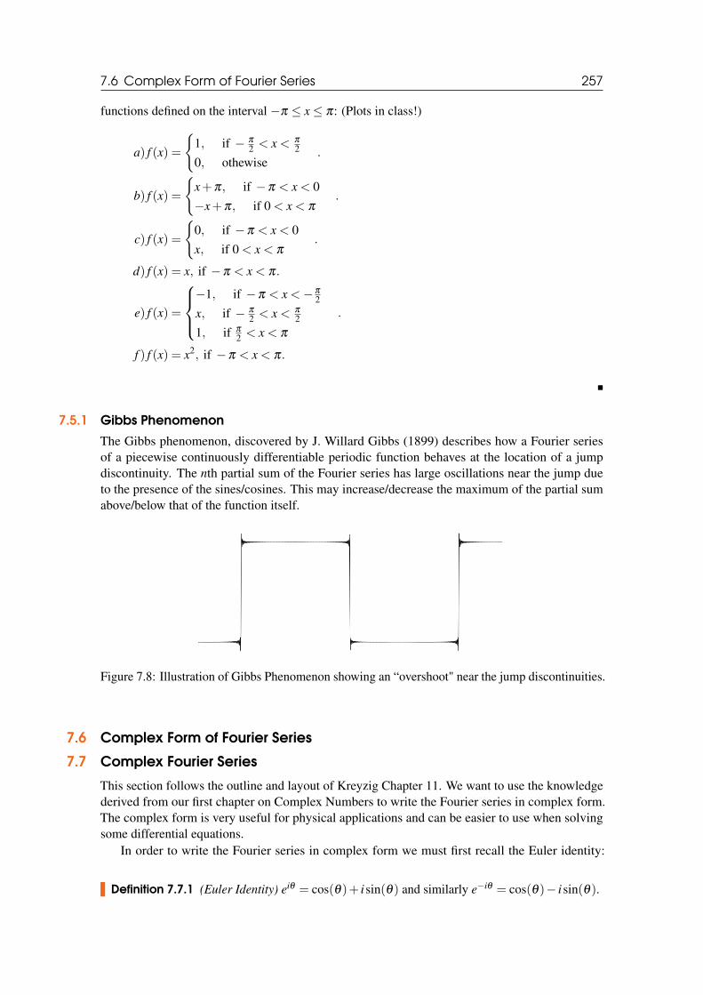
7.6 Complex Form of Fourier Series 257
functions defined on the interval −π ≤ x≤ π: (Plots in class!)
a) f (x) =
1, if − π
2 < x < π
2
0, othewise.
b) f (x) =
x+π, if −π < x < 0−x+π, if 0 < x < π
.
c) f (x) =
0, if −π < x < 0x, if 0 < x < π
.
d) f (x) = x, if −π < x < π.
e) f (x) =
−1, if −π < x <−π
2
x, if − π
2 < x < π
2
1, if π
2 < x < π
.
f ) f (x) = x2, if −π < x < π.
7.5.1 Gibbs Phenomenon
The Gibbs phenomenon, discovered by J. Willard Gibbs (1899) describes how a Fourier seriesof a piecewise continuously differentiable periodic function behaves at the location of a jumpdiscontinuity. The nth partial sum of the Fourier series has large oscillations near the jump dueto the presence of the sines/cosines. This may increase/decrease the maximum of the partial sumabove/below that of the function itself.
Figure 7.8: Illustration of Gibbs Phenomenon showing an “overshoot" near the jump discontinuities.
7.6 Complex Form of Fourier Series
7.7 Complex Fourier Series
This section follows the outline and layout of Kreyzig Chapter 11. We want to use the knowledgederived from our first chapter on Complex Numbers to write the Fourier series in complex form.The complex form is very useful for physical applications and can be easier to use when solvingsome differential equations.
In order to write the Fourier series in complex form we must first recall the Euler identity:
Definition 7.7.1 (Euler Identity) eiθ = cos(θ)+ isin(θ) and similarly e−iθ = cos(θ)− isin(θ).

258 Chapter 7. Fourier Series and Transforms
Also, recall by adding and subtracting these functions we get the complex form of the sine andcosine functions
cos(t) =12(eit + e−it), sin(t) =
12i(eit − e−it). (7.14)
Recall 1/i =−i and let t = nx to find
an cos(nx)+bn sin(nx) =12
an(einx + e−inx)+12i
bn(einx− e−inx)
=12(an− ibn)einx +
12(an + ibn)e−inx.
Inputting this expression into the Fourier series while writing a0 = c0,12(an− ibn) = cn,
12(an +
ibn) = kn to find
f (x) = a0 +∞
∑n=1
[cneinx + kne−inx] . (7.15)
where the coefficients ci,ki are defined as
cn =12(an− ibn) =
12π
∫π
−π
f (x) [cos(nx)− isin(nx)]dx =1
2π
∫π
−π
f (x)e−inxdx
kn =12(an + ibn) =
12π
∫π
−π
f (x) [cos(nx)+ isin(nx)]dx =1
2π
∫π
−π
f (x)einxdx.
We simply the formula further by setting c−n = kn, then the Fourier series can be written as:
f (x) =∞
∑n=−∞
cneinx, cn =1
2π
∫π
−π
f (x)e−inxdx, n = 0,±1,±2, ... (7.16)
This is the complex form of the Fourier series of the Complex Fourier series of f (x). The cn arethe complex Fourier coefficients of f (x).
Example 7.10 Find the complex Fourier series of f (x) = ex if−π < x < π and f (x+2π) = f (x)and then from it obtain the usual Fourier series as a check.
Solution: Start by computing the complex Fourier coefficients:
cn =1
2π
∫π
−π
exe−inxdx =1
2π
11− in
ex−inx∣∣∣∣π−π
=1
2π
11− in
(eπ − e−π)(−1)n.
On the right side, 11−in = 1+in
1+n2 and eπ − e−π = 2sinh(π). Hence the complex Fourier series is
ex =sinh(π)
π
∞
∑n=−∞
(−1)n 1+ in1+n2 einx. (7.17)
Now, derive the traditional Fourier series. Notice that
(1+ in)einx = (1+ in) [cos(nx)+ isin(nx)] = [cos(nx)−nsin(nx)]+ i [ncos(nx)+ sin(nx)]
(1− in)e−inx = (1− in) [cos(nx)− isin(nx)] = [cos(nx)−nsin(nx)]− i [ncos(nx)+ sin(nx)]
Adding these to equations results in the imaginary parts canceling
(1+ in)einx +(1− in)e−inx = 2 [cos(nx)−nsin(nx)] , n = 1,2, ...
for n = 0 we get 1. Thus, the real Fourier series is
ex =2sinh(π)
π
[12− 1
1+12 [cos(x)− sin(x)]+1
1+22 [cos(2x)−2sin(2x)]− ...
].

7.7 Complex Fourier Series 259
Figure 7.9: Plot of the partial sum for the Fourier series of ex.
Example 7.11 Find the complex Fourier series of f (x) = sin(x) if −π < x < π and f (x+2π) =f (x).
Solution: Start by computing the complex Fourier coefficients:
cn =1
2π
∫π
−π
sin(x)e−inxdx =1
2π
[einπ − e−inπ
n2−1
].
The coefficients are zero unless n = ±1 (since e±inπ = cos(nπ)± isin(nπ) = cos(nπ) = (−1)n.Using L’Hospital rule twice gives c1 =
12i and c−1 =− 1
2i . Thus, the complex Fourier series is
f (x) =∞
∑n=−∞
cneinx =eix− e−ix
2i,
which is exactly the complex representation of the sine function.
Example 7.12 Find the complex Fourier series of f (x) = 1 if 0 < x < T , f (x) = 0 otherwise,and f (x+2π) = f (x).
Solution: Start by computing the complex Fourier coefficients:
cn =1
2π
∫π
−π
f (x)e−inxdx =1
2π
∫ T
0e−inxdx =
i2πn
e−inx∣∣∣∣T0=
i2πn
[einT −1
],
when n 6= 0. Also, c0 =1
2π
∫ T0 dx = T
2π. Thus, the complex Fourier series is
f (x) =∞
∑n=−∞
cneinx =1
2π
[T +
∞
∑n=−∞,n6=0
in
[e−inT −1
]einx
].
7.7.1 General Complex Fourier Series for Intervals (0,L)Definition 7.7.2 The complex Fourier series for an interval from (0,L) has the form
f (x) =∞
∑n=−∞
cneinx 2π
L , cn =1L
∫ L
0e−inx 2π
L f (x)dx. (7.18)
The fraction 2π
L is often written as ω0 and called the fundamental angular frequency.

260 Chapter 7. Fourier Series and Transforms
Example 7.13 Find the complex Fourier series of f (x) = 1 if 0 < x < L/2, f (x) = −1 ifL/2 < x < L, and f (x+2π) = f (x).
Solution: Start by computing the complex Fourier coefficients:
cn =1L
∫ L
0e−inx 2π
L f (x)dx =1L
[∫ L/2
0e−inx 2π
L dx−∫ L
L/2e−inx 2π
L dx]=
i2πin
[e−2inπ +1−2−inπ
],
when n 6= 0. Also, c0 = 0 since the mean of the function is zero. Thus, the complex Fourier series is
f (x) =∞
∑n=−∞
cneinx =∞
∑n=−∞,n6=0
[1− e−inπ ]
inπeinx 2π
L .
Example 7.14 Find the complex Fourier series for the following functions a) f (x) = 1 for−π < x < π , b) f (x) =−2x for −π < x < π .
Solution: For a)
cn =1
2π
∫π
−π
e−inxdx =− 12πin
e−inx∣∣∣∣π−π
=− 12πin
[e−inπ − einπ
],
which is 0 when n 6= 0. Thus the only term in the Fourier series is c0 = 1.
For b)
cn =1
2π
∫π
−π
xe−inxdx =1
2π
[−xin
e−inx∣∣∣∣π−π
−∫
π
−π
−1in
e−inxdx]
=1
2π
[−π
in[2einπ ]+
1n2 e−inx
∣∣∣∣π−π
]=
12π
[−π
in[2einπ ]+
1n2 [e
−inπ − e−inπ ]
]If n 6= 0, then cn = − 1
2in 2einπ = in einπ . If n = 0, then c0 = 1
2π
∫π
−πxdx = 0. Thus, the complex
Fourier series is
f (x) =∞
∑n=−∞
cneinx =∞
∑n=−∞,n6=0
in
einπeinx =∞
∑n=−∞,n6=0
in
ein(π+x).
7.8 General Fourier Series for Functions of Any Period p = 2L
This section follows the outline and layout of Kreyzig Chapter 11. So far all the functions consid-ered have had period p = 2π simplifying the formulas for the Fourier coefficients and the Fourierseries. In general for applications, most functions do not have period 2π , but rather possess a periodof arbitrary length we will call p = 2L. The good news is that the Fourier series and formulas forthe coefficients for a general function of period 2L have a very similar form. We use the notationp = 2L where L is the length of the object under consideration (such as a spring or rod). We willsee this application in the Chapter on PDEs.

7.8 General Fourier Series for Functions of Any Period p = 2L 261
Key Idea: Find and use a change of scale that transforms a 2π periodic function into a func-tion of period 2L. Recall, the form of the for a function of period 2π
g(v) = a0 +∞
∑n=1
[an cos(nv)+bn sin(nv)] (7.19)
with coefficients
a0 =1
2π
∫π
−π
g(v)dv (7.20)
an =1π
∫π
−π
g(v)cos(nv)dv n = 1,2,3, ... (7.21)
bn =1π
∫π
−π
g(v)sin(nv)dv n = 1,2,3, .... (7.22)
Using a change of scale, let v = kx with k such that the old period v = 2π and gives a new periodwhere x = 2L. Thus, 2π = k2L⇒ k = π/L. Therefore, v = kx = πx/L and dv = π
L dx. Now writingg(v) = f (x), the Fourier series and coefficients become
f (x) =a0
2+
∞
∑n=1
[an cos
(nπ
Lx)+bn sin
(nπ
Lx)]
(7.23)
with coefficients
a0 =1
2L
∫ L
−Lf (x)dx (7.24)
an =1L
∫ L
−Lf (x)cos
(nπxL
)dx n = 1,2,3, ... (7.25)
bn =1L
∫ L
−Lf (x)sin
(nπxL
)dx n = 1,2,3, .... (7.26)
Also, the complex Fourier series can be expressed for arbitrary intervals
f (x) =∞
∑n=−∞
cne−nπx
L , cn =1
2L
∫ L
−Lf (x)e−
inπ
x dx. (7.27)
Example 7.15 (Periodic Rectangular Wave) Find the Fourier series of the function
f (x) =
0 if −2 < x <−1k if −1 < x < 10 if 1 < x < 2
,
where p = 2L = 4 and L = 2.
Solution: Using the formulas just derived we can find the Fourier coefficients
a0 =1
2L
∫ L
−Lf (x)dx =
14
∫ 1
−1kdx =
k4
x∣∣∣∣1−1
=k2
an =1L
∫ L
−Lf (x)cos
(nπxL
)dx =
12
∫ 1
−1k cos
(nπx2
)dx
=k
nπsin(nπx
2
)∣∣∣∣1−1
=2knπ
sin(nπ
2
)bn =
1L
∫ L
−Lf (x)sin
(nπxL
)dx =
12
∫ 1
−1k sin
(nπx2
)dx
=− knπ
cos(nπx
2
)∣∣∣∣1−1
=− knπ
[cos(nπ
2
)− cos
(−nπ
2
)]= 0

262 Chapter 7. Fourier Series and Transforms
Observe that an = 0 if n is even. Hence the Fourier series is
f (x) =k2+
2kπ
[cos(
π
2x)− 1
3cos(
3π
2x)+
15
cos(
5π
2x)+ ...
].
Figure 7.10: Period Rectangular Wave from first example.
Example 7.16 (Periodic Rectangular Wave) Find the Fourier series of the function
f (x) =
−k if −2 < x < 0k if 0 < x < 2
,
where p = 2L = 4 and L = 2.
Solution: Using the formulas just derived we can find the Fourier coefficients
a0 =1
2L
∫ L
−Lf (x)dx =
14
[∫ 0
−2−kdx+
∫ 2
0kdx]=
k4
x∣∣∣∣0−2
+k4
x∣∣∣∣20= 0
an =1L
∫ L
−Lf (x)cos
(nπxL
)dx =
12
[∫ 0
−2−k cos
(nπx2
)dx+
∫ 2
0k cos
(nπx2
)dx]
=12
[− 2k
nπsin(nxπ
2
)∣∣∣∣0−2
+2knπ
sin(nπx
2
)∣∣∣∣20
]= 0
bn =1L
∫ L
−Lf (x)sin
(nπxL
)dx =
12
[∫ 0
−2−k sin
(nπx2
)dx+
∫ 2
0k sin
(nπx2
)dx]
=12
[2knπ
cos(nxπ
2
)∣∣∣∣0−2− 2k
nπcos(nπx
2
)∣∣∣∣20
]
=k
nπ[1− cos(nπ)− cos(nπ)+1] =
4k/nπ if n is odd0 if n is even
.
Hence the Fourier series is
f (x) =4kπ
[sin(
π
2x)+
13
sin(
3π
2x)+
15
sin(
5π
2x)+ ...
].
Example 7.17 (Half-wave Rectifier) Find the Fourier series of the function
f (x) =
0 if −L < t < 0E sin(ωt) if 0 < x < L
,

7.8 General Fourier Series for Functions of Any Period p = 2L 263
Figure 7.11: Period Rectangular Wave from second example.
where p = 2L = 2π
ωand L = π
ω.
Solution: Using the formulas just derived we can find the Fourier coefficients
a0 =1
2L
∫ L
−Lf (t)dt =
ω
2π
∫π/ω
0E sin(ωt)dt =
Eπ
an =1L
∫ L
−Lf (t)cos
(nπtL
)dt =
ω
π
∫π/ω
0E sin(ωt)cos(nωt)dt
=ωE2π
∫π/ω
0[sin((1+n)ωt)+ sin((1−n)ωt)]dt
=ωE2π
[−cos((1+n)ωt)
(1+n)ω− cos((1−n)ωt)
(1−n)ω
]π/ω
0=
E2π
[−cos((1+n)π)+1
1+n+−cos((1−n)π)+1
1−n
]bn =
1L
∫ L
−Lf (t)sin
(nπtL
)dt =
ω
π
∫π/ω
0E sin(ωt)sin(nωt)dt.
Observe that a1 = 0 and an = 0 is n is odd. For n even, an =E2π
( 21+n +
21−n
)=− 2E
(n−1)(n+1)π . Also,b1 = E/2 and all other bn = 0. Hence the Fourier series is
f (t) =Eπ+
E2
sin(ωt)− 2Eπ
[1
1 ·3cos(2ωt)+
13 ·5
cos(4ωt)+ ...
].
Figure 7.12: Half-wave Rectifier from second example.
Example 7.18 Compute the Fourier Series of f (x) = 1+ x on the interval (−L,L).

264 Chapter 7. Fourier Series and Transforms
Solution: Using the above formulas we have
a0 =1
2L
∫ L
−L(1+ x)dx = 1
am =1L
∫ L
−L(1+ x)cos(
mπxL
)dx
=1+ xmπ
sin(mπx
L)+
1m2π2 cos(
mπxL
)|L−L
=1
m2π2 (cos(mπ)− cos(−mπ)) = 0 m 6= 0
bm =1L
∫ L
−L(1+ x)sin(
mπxL
)dx
= −1+ xmπ
cos(mπx
L)+
1m2π2 sin(
mπxL
)|L−L
= − 2Lmπ
cos(mπ) = (−1)m+1 2Lmπ
.
So the full Fourier series of f (x) is
1+ x = 1+2Lπ(sin(
πxL)− 1
2sin(
2πxL
)+13
sin(3πx
L)− ...) (7.28)
= 1+2Lπ
∞
∑n=1
12n−1
sin((2n−1)πx
L)− 1
2nsin(
2nπxL
). (7.29)
Example 7.19 Compute the Fourier Series for f (x) =
2 −2≤ x <−11− x −1≤ x < 2
on the interval
(−2,2).
Solution: We start by using the Euler-Fourier Formulas. For the Cosine terms we find
a0 =14
∫ 2
−2f (x)dx
=14
(∫ −1
−22dx+
∫ 2
−11− xdx
)=
14(2+
32) =
78
and
an =12
∫ 2
−2f (x)cos(
nπx2
)dx
=12
(∫ −1
−22cos(
nπx2
)dx+∫ 2
−1(1− x)cos(
nπx2
)dx)
=12
(4
nπsin(
nπx2
)|−1−2 +
2(1− x)nπ
sin(nπx
2)|2−1−
4n2π2
(cos(
nπx2
)|2−1
))=
12
(− 4
nπsin(
nπ
2)+
4nπ
sin(nπ
2)− 4
n2π2 (cos(nπ)− cos(nπ
2))
)
=
2
n2π2 n odd0 n = 4m− 4
n2π2 n = 4m+2
.

7.9 Even and Odd Functions 265
Also, for the sine terms
bn =12
∫ 2
−2f (x)sin(
nπx2
)dx
=12
(∫ −1
−22sin(
nπx2
)dx+∫ 2
−1(1− x)sin(
nπx2
)dx)
=12
(− 4
nπcos(
nπx2
)|−1−2−
2(1− x)nπ
cos(nπx
2)|2−1−
4n2π2 (sin(
nπx2
)|2−1
)=
12
(6
nπcos(nπ)− 4
n2π2 sin(nπ
2)
)
=
3
nπneven
− 3nπ− 2
n2π2 n = 4m+1− 3
nπ+ 2
n2π2 n = 4m+3
.
So we have
f (x) =78
+∞
∑m=1
2(4m+1)2π2 cos
((4m+1)πx
2
)+
(− 3(4m+1)π
− 2(4m+1)2π2
)sin((4m+1)πx
2
)− 4
(4m+2)2π2 cos((4m+2)πx
2
)+
3(4m+2)π
sin((4m+2)πx
2
)+
2(4m+3)2π2 cos
((4m+3)πx
2
)+
(− 3(4m+3)π
+2
(4m+3)2π2
)sin((4m+3)πx
2
)+
34mπ
sin(
4mπx2
).
This example represents a worst case scenario. There are a lot of Fourier coefficients to keeptrack of. Notice that for each value of m, the summand specifies four different Fourier terms (for4m,4m+1,4m+2,4m+3). This can often happen and depending on L, even more terms mayberequired.
7.9 Even and Odd Functions
7.10 Even and Odd Functions, Half-Range ExpansionsRecall that an even function is a function satisfying
g(−x) = g(x). (7.30)
This means that the graph y = g(x) is symmetric with respect to the y-axis. An odd functionsatisfies
g(−x) =−g(x) (7.31)
meaning that its graph y = g(x) is symmetric with respect to the origin.
Example 7.20 A monomial xn is even if n is even and odd if n is odd. cos(x) is even and sin(x)is odd. Note tan(x) is odd.
There are some general rules for how products and sums behave:(1) If g(x) is odd and h(x) is even, their product g(x)h(x) is odd.(2) If g(x) and h(x) are either both even or both odd, g(x)h(x) is even.

266 Chapter 7. Fourier Series and Transforms
Figure 7.13: Even function (Left) and Odd function (Right).
(3) The sum of two even functions or two odd functions is even or odd, respectively.To remember the rules consider how many negative signs come out of the arguments.(4) The sum of an even and an odd function can be anything. In fact, any function on (−L,L) canbe written as a sum of an even function, called the even part, and an odd function, called the oddpart.(5) Differentiation and Integration can change the parity of a function. If f (x) is even, d f
dx and∫ x0 f (s)ds are both odd, and vice versa.
The graph of an odd function g(x) must pass through the origin by definition. This also tells usthat if g(x) is even, as long as g′(0) exists, then g′(0) = 0.
Theorem 7.10.1 Definite Integrals on symmetric intervals of odd and even functions have usefulproperties∫ L
−L(odd)dx = 0 and
∫ L
−L(even)dx = 2
∫ L
0(even)dx (7.32)
Given a function f (x) defined on (0,L), there is only one way to extend it to (−L,L) to an evenor odd function. The even extension of f (x) is
feven(x) =
f (x) for 0 < x < Lf (−x) for −L < x < 0.
(7.33)
This is just its reflection across the y-axis. Notice that the even extension is not necessarily definedat the origin.
The odd extension of f (x) is
fodd(x) =
f (x) for 0 < x < L− f (−x) for −L < x < 00 for x = 0
. (7.34)
This is just its reflection through the origin.
R Since the cosine terms in a Fourier series are even and the sine terms are odd, then it shouldnot be surprising that an even function is given by a series of cosine terms and an odd functionby a series of sine terms.

7.10 Even and Odd Functions, Half-Range Expansions 267
Theorem 7.10.2 (Fourier Cosine Series, Fourier Sine Series) The Fourier series of an evenfunction of period 2L is a Fourier Cosine Series
f (x) = a0 +∞
∑n=1
an cos(nπ
Lx)
(7.35)
with coefficients (NOTE: Integration only on the half-interval (0,L)!)
a0 =1L
∫ L
0f (x)dx
an =2L
∫ L
0f (x)cos
(nπxL
)dx, n = 1,2,3, ...
The Fourier series of an odd function of period 2L is a Fourier Sine Series
f (x) =∞
∑n=1
bn sin(nπx
L
)(7.36)
with coefficients
bn =2L
∫ L
0f (x)sin
(nπxL
)dx.
Theorem 7.10.3 (Sum and Scalar Multiple) The Fourier coefficients of a sum f1 + f2 are thesums of the corresponding Fourier coefficients of f1 and f2. The Fourier coefficients of c f are ctimes the Fourier coefficients of f .
Figure 7.14: Sawtooth function.
Example 7.21 (Sawtooth Wave) Find the Fourier series of the function f (x) = x+π if −π <x < π and f (x+2π) = f (x).
Solution: Here we have f = f1 + f2 where f1 = x and f2 = π . The Fourier coefficients of f2are zero except for the first one (the constant term, a0 = π). Thus, the Fourier coefficients an,bn arethose for f1 except for a0, which is π . Since f1 is odd, then an = 0 for n = 1,2, ... and
bn =2π
∫π
0f1(x)sin(nx)dx =
2π
∫π
0xsin(nx)dx
=2π
[−xcos(nx)
n
∣∣∣∣π0+
1n
∫π
0cos(nx)dx
]=−2
ncos(nπ).

268 Chapter 7. Fourier Series and Transforms
Thus, b1 = 2,b2 =−2/2 =−1,b3 = 2/3,b4 =−2/4 =−1/2, ... and the Fourier series of f (x) is
f (x) = π +2(
sin(x)− 12
sin(2x)+13
sin(3x)− ...
).
Figure 7.15: First few partial sums.
7.10.1 Half-Range Expansions
Half-range expansions are Fourier series. The basic idea is to represent a function f (x) by a Fourierseries where the function is only defined on the interval (0,L). This could represent a violin stringor the temperature distribution in a metal bar. We could extend f (x) as a function of period L anddevelop the extended function into a Fourier Series. This series would in general contain both sineand cosine terms requiring many computations. We know that if the function were even on (−L,L)we would only have to compute the cosine terms. Likewise if the function were odd on the interval(−L,L) then we would only need to compute the cosine terms.
Definition 7.10.1 An even periodic extension is a function of period 2L which is even, butcoincides with the given function f (x) on the interval (0,L) (see f1 in figure).
An odd periodic extension is a function of period 2L which is odd, but coincides withthe given function f (x) on the interval (0,L) (see f2 in figure).
R Both extensions have period 2L. This is where the term half-range expansion comes from:f is given on half the range (0,L) giving only half the periodicity of the length 2L.
Example 7.22 Find the two half-range expansions for the function
f (x) =
2kL x if 0 < x < L
22kL (L− x) if L
2 < xL.
Solution: a) Even Periodic Extension: Find the Fourier Cosine series, which converges to the even

7.10 Even and Odd Functions, Half-Range Expansions 269
Figure 7.16: Extensions to even and odd functions. f1(x) is the even periodic extension and f2(x)is the odd periodic extension.
periodic extension. Start by finding the Fourier coefficients:
a0 =1L
[2kL
∫ L/2
0xdx+
2kL
∫ L
L/2(L− x)dx
]=
k2
an =2L
[2kL
∫ L/2
0xcos
(nπ
Lx)
dx+2kL
∫ L
L/2(L− x)cos
(nπ
Lx)
dx]
=IBPL2
2nπsin(nπ
2
)+
L2
n2π2
(cos
nπ
2−1)− L
nπ
(L− L
2
)sin(nπ
2
)− L2
n2π2
(cos(nπ)− cos
nπ
2
).
Combining the terms in an gives an =4k
n2π2
(2cos nπ
2 − cos(nπ)−1)
and an = 0 if n= 2,6,10, ...,4n−2, .... Hence, the first half-range expansion of f (x) is
f (x) =k2− 16k
π2
(122 cos
2π
Lx+
162 cos
6π
Lx+ ...
).
b) Odd Period Extension: Find the Fourier Sine series, which converges to the odd periodicextension. Start by finding the Fourier coefficients:
bn =8k
n2π2 sinnπ
2.
Thus, the other half-range expansion of f (x) is
f (x) =8kπ2
(112 sin
π
Lx− 1
32 sin3π
Lx+
152 sin
5π
Lx− ...
).
7.10.2 Fourier Sine SeriesEach of terms in the Fourier Sine Series for f (x), sin(nπx
L ), is odd. As with the full Fourier Series,each of these terms also has period 2L. So we can think of the Fourier Sine Series as the expansionof an odd function with period 2L defined on the entire line which coincides with f (x) on (0,L).

270 Chapter 7. Fourier Series and Transforms
Figure 7.17: Even and odd extensions.
One can show that the full Fourier Series of fodd is the same as the Fourier Sine Series of f (x).Let
a0 +∞
∑n=1
an cos(nπx
L)+bn sin(
nπxL
) (7.37)
be the Fourier Series for fodd(x), with coefficients given in Section 10.3
an =1L
∫ L
−Lfodd(x)cos(
nπxL
)dx = 0 (7.38)
But fodd is odd and cos is even, so their product is again odd.
bn =1L
∫ L
−Lfodd(x)sin(
nπxL
)dx (7.39)
But both fodd and sin are odd, so their product is even.
bn =2L
∫ L
0fodd(x)sin(
nπxL
)dx (7.40)
=2L
∫ L
0f (x)sin(
nπxL
)dx, (7.41)
which are just the Fourier Sine coefficients of f (x). Thus, as the Fourier Sine Series of f (x) is thefull Fourier Series of fodd(x), the 2L-periodic odd function that the Fourier Sine Series expands isjust the periodic extension fodd .
This goes both ways. If we want to compute a Fourier Series for an odd function on (−L,L) wecan just compute the Fourier Sine Series of the function restricted to (0,L). It will almost convergeto the original function on (−L,L) with the only issues occurring at any jump discontinuities. Theonly works for odd functions. Do not use the formula for the coefficients of the Sine Series,unless you are working with an odd function.
Example 7.23 Write down the odd extension of f (x) = L− x on (0,L) and compute its FourierSeries.
Solution: To get the odd extension of f (x) we will need to see how to reflect f across theorigin. What we end up with is the function
fodd(x) =
L− x 0 < x < L−L− x −L < x < 0
. (7.42)

7.10 Even and Odd Functions, Half-Range Expansions 271
Now, what is the Fourier Series of fodd(x)? By the previous discussion, we know that is will beidentical to the Fourier Sine Series of f (x), as this will converge on (−L,0) to fodd . So we have
fodd(x) =∞
∑n=1
bn sin(nπx
L), (7.43)
where
bn =2L
∫ L
0(L− x)sin(
nπxL
)dx (7.44)
=2L[−L(L− x)
nπcos(
nπxL
)− L2
n2π2 sin(nπx
L)]L0 (7.45)
=2Lnπ
. (7.46)
Thus the desired Fourier Series is
fodd(x) =2Lπ
∞
∑n=1
1n
sin(nπx
L). (7.47)
Can we compute the Fourier Sine Series of a constant function like f (x) = 1 which is even? Itis important to remember that if we are computing the Fourier Sine Series for f (x), it only needs toconverge to f (x) on (0,L), where issues of evenness and oddness do not occur. The Fourier SineSeries will converge to the odd extension of f (x) on (−L,L).
Example 7.24 Find the Fourier Series for the odd extension of
f (x) =
32 0 < x < 3
2
x− 32
32 < x < 3.
(7.48)
on (−3,3).
Solution: The Fourier Series for fodd(x) on (−3,3) will just be the Fourier Sine Series for f (x) on(0,3). The Fourier Sine coefficients for f (x) are
bn =23
∫ 3
0f (x)sin(
nπx3
)dx (7.49)
=23
(∫ 32
0
32
sin(nπx
3)dx+
∫ 3
32
(x− 32)sin(
nπx3
)
)(7.50)
=23
(− 9
2nπcos(
nπx3
)|320 +
3(x− 32)
nπcos(
nπx3
)|332+
9n2π2 sin(
nπx3
)|332
)(7.51)
=23
(− 9
2nπ(cos(
nπ
2)−1)− 9
2nπcos(nπ)− 9
n2π2 sin(nπx
2)
)(7.52)
=23(
92nπ
(1− cos(nπ
2)+(−1)n+1)− 9
n2π2 sin(nπ
2)
)(7.53)
=3
nπ
(1− cos(
nπ
2)+(−1)n+1− 2
nπsin(
nπ
2)
)(7.54)
and the Fourier Series is
fodd(x) =3π
∞
∑n=1
1n[1− cos(
nπ
2)+(−1)n+1− 2
nπsin(
nπ
2)]sin(
nπx3
). (7.55)
272 Chapter 7. Fourier Series and Transforms
7.10.3 Fourier Cosine Series
Now consider what happens for the Fourier Cosine Series of f (x) on (0,L). This is analogous tothe Sine Series case. Every term in the Cosine Series has the form
an cos(nπx
L) (7.56)
and hence is even, so the entire Cosine Series is even. Thus, the Cosine Series must converge on(−L,L) to an even function which coincides on (0,L) with f (x). This must be the even extension
feven(x) =
f (x) 0 < x < Lf (−x) −L < x < 0
. (7.57)
Notice that this definition does not specify the value of the function at zero, the only restriction onan even function at zero is that, if it exists, the derivative should be zero.
It is straight forward enough to show that the Fourier coefficients of feven(x) coincide with theFourier Cosine coefficients of f (x). The Euler-Fourier formulas give
an =1L
∫ L
−Lfeven(x)cos(
nπxL
)dx (7.58)
=2L
∫ L
0feven(x)cos(
nπxL
)dx since feven(x)cos(nπx
L) is even (7.59)
=2L
∫ l
0feven(x)cos(
nπxL
)dx (7.60)
which are the Fourier Cosine coefficients of f (x) on (0,L)
bn =1L
∫ L
−Lfeven(x)sin(
nπxL
)dx = 0 (7.61)
since feven(x)sin(nπxL ) is odd. Thus the Fourier Cosine Series of f (x) on (0,L) can be considered
as the Fourier expansion of feven(x) on (−L,L), and therefore also as expansion of the periodicextension of feven(x). It will converge as in the Fourier Convergence Theorem to this periodicextension.
This also means that if we want to compute the Fourier Series of an even function, we can justcompute the Fourier Cosine Series of its restriction to (0,L). It is very important that this only beattempted if the function we are starting with is even.
Example 7.25 Write down the even extension of f (x) = L− x on (0,L) and compute its FourierSeries.
Solution: The even extension will be
feven(x) =
L− x 0 < x < LL+ x −L < x < 0
. (7.62)
Its Fourier Series is the same as the Fourier Cosine Series of f (x), by the previous discussion. Sowe can just compute the coefficients. Thus we have
feven(x) = a0 +∞
∑n=1
an cos(nπx
L), (7.63)

7.10 Even and Odd Functions, Half-Range Expansions 273
where
a0 =1L
∫ L
0f (x)dx =
1L
∫ L
0(L− x)dx =
L2
(7.64)
an =2L
∫ L
0f (x)cos(
nπxL
)dx (7.65)
=2L
∫ L
0(L− x)cos(
nπxL
)dx (7.66)
=2L[L(L− x)
nπsin(
nπxL
)− L2
n2π2 cos(nπx
L)]L0 (7.67)
=2L
(L2
n2π2 (−cos(nπ)+ cos(0)))
(7.68)
=2L
n2π2 ((−1)n+1 +1). (7.69)
So we have
feven(x) =L2+
∞
∑n=1
2Ln2π2 ((−1)n+1 +1). (7.70)
Example 7.26 Write down the even extension of
f (x) =
32 0≤ x < 3
2
x− 32
32 ≤ x≤ 3
(7.71)
and compute its Fourier Series.
Solution: Using Equation (7.57) we see that the even extension is
feven(x) =
x− 3
232 < x < 3
32 0≤ x < 3
232 − 3
2 < x < 0−x− 3
2 −3≤ x≤−32
. (7.72)

274 Chapter 7. Fourier Series and Transforms
We just need to compute the Fourier Cosine coefficients of the original f (x) on (0,3).
a0 =13
∫ 3
0f (x)dx (7.73)
=13
(∫ 3/2
0
32
dx+∫ 3
3/2x− 3
2dx)
(7.74)
=13(94+
98) =
98
(7.75)
an =23
∫ 3
0f (x)cos(
nπx3
)dx (7.76)
=23
(∫ 3/2
0
32
cos(nπx
3)dx+
∫ 3
3/2(x− 3
2)cos(
nπx3
)dx)
(7.77)
=23
(9
2nπsin(
nπx3
)|3/20 +
3(x− 32)
nπsin(
nπx3
)|33/2 +9
n2π2 cos(nπx
3)|33/2
)(7.78)
=23
(9
2nπsin(
nπ
2)+
9n2π2
(cos(nπ)− cos(
nπ
2)
))(7.79)
=6
nπ
(12
sin(nπ
2)+
1nπ
((−1)n− cos(
nπ
2)
))(7.80)
=6
nπ
(1
nπ((−1)n− cos(
nπ
2))+
12
sin(nπ
2)
). (7.81)
So the Fourier Series is
feven =98+
6π
∞
∑n=1
1n
(1
nπ
((−1)n− cos(
nπ
2))+
12
sin(nπ
2)
)cos(
nπx3
). (7.82)

8. Partial Differential Equations
8.1 Introduction to Basic Classes of PDEs
8.2 Introduction to PDEs
Many physical and geometric problems rely on models formed by partial differential equations(PDEs). Here the known functions depend on more than one variable, for example space and time.In previous chapters we studied ODEs equations which have limited use in modeling physicalsystems. Usually they are restricted to the simplest situations such as spring-mass systems orpopulation dynamics. Now we wish to consider problems form a wider range of fields such aselasticity, thermodynamics, electrostatics, quantum mechanics, and population dynamics.
Throughout the remainder of the Chapter we focus on initial value problems (IVP) and boundaryvalue problems (BVP) for common physical systems such as a vibrating string, temperaturedistribution in a material, or an elastic membrane.
In this section, we briefly outline the basic concepts involved in studying PDEs and the sixmost basic PDEs common to math and physics and describe the physical situations where eachcomes about.
8.2.1 Basics of Partial Differential EquationsDefinition 8.2.1 A partial differentiation equation (PDE) is an equation involving one ormore partial derivatives of an unknown function that depends on more than one variable.
Definition 8.2.2 The order of a PDE is the order of the highest derivative.
Definition 8.2.3 A PDE is linear if it is of the first degree in the unknown function and itspartial derivatives, otherwise we call it nonlinear.
R The remainder of the course focuses on second order linear PDEs, which have a surprisinglywide range of applications.

276 Chapter 8. Partial Differential Equations
Example 8.1 Determine if the following PDEs are linear and what their order is:
• uxx+2uux = 3• uxxx + sin(u) = 0• ux +3u = 5sin(x)• (ux)
3 +uxx = x3
Definition 8.2.4 We call a linear PDE homogeneous if each of its terms contains either u orone of its partial derivatives, otherwise we call the equation nonhomogeneous.
Example 8.2 In the previous example determine which of the equations is homogeneous.
8.2.2 Laplace’s Equation - Type: Elliptical∆u = 0 (8.1)
Applications include gravitational potential u in a region with no mass, electrostatic potential ina charge free region, the steady state temperature distribution in a region without sources or sinks,or the velocity of an incompressible fluid with no vortices or sinks.
8.2.3 Poisson’s Equation∆u = f (x,y,z) (8.2)
Applications include everything for Laplace, but f represents a source term either charge,electrical, force, or heat source.
8.2.4 Diffusion/Heat Equation - Type: Parabolic
∆u =1
α2∂u∂ t
(8.3)
The quantity u can represent a non-steady state temperature distribution in a region withoutheat sources, concentration of a diffusing substance. Here α2 is known as the thermal diffusivity.
8.2.5 Wave Equation - Type: Hyperbolic
∆u =1v2
∂ 2u∂ t2 (8.4)
The quantity u represents displacement from equilibrium of a vibrating string or membrane, inelectrostatics it can be the current or potential along a transmission line, or u can be the componentof the electric or magnetic field in an electromagnetic wave.
8.2.6 Helmholtz Equation∆F + k2F = 0 (8.5)
The time-independent form of the wave equation.
8.2.7 Schrödinger Equation
=h
2m∆Ψ+V Ψ = ih
∂
∂ tΨ (8.6)
The wave equation of quantum mechanics where m is the particle mass, h is Planck’s constant,i =√−1, and V is the potential energy of the particle. The wave function Ψ is complex and its
absolute value squared is proportional to the position probability of the particle.

8.3 Laplace’s Equations and Steady State Temperature Problems 277
8.2.8 Solutions to PDEsDefinition 8.2.5 A solution of a PDE in some region R of the space of the independent variablesis a function that has all the partial derivatives appearing in the PDE in some domain D containingR, and satisfies the PDE everywhere in R.
R Solutions to the same equation can look very different. Consider the PDE
∂ 2u∂x2 +
∂ 2u∂y2 = 0.
The following five functions are all solutions (verify): 1. u = x2 − y2, 2. ex cos(y), 3.u = sin(x)cosh(y), 4. u = 5, 5. u = ln(x2 + y2). A unique solution is obtained by combiningthe PDE with initial and/or boundary conditions.
Definition 8.2.6 If there is a condition prescribing the values of the unknown function u on theboundary of domain R, we call these conditions boundary conditions. When t is one of thevariables we can describe the unknown function u or its derivatives at time t = 0, we call theseconditions initial conditions.
Theorem 8.2.1 (Principle of Superposition) If u1 and u2 are solutions of a homogeneous linearPDE in some region R, then
u = c1u1 + c2u2 (8.7)
with any constants c1,c2 is also a solution of that PDE in the region R.
Example 8.3 (Similar to ODE) Find solutions u of the PDE uxx−u = 0 where u = u(x,y).
Solution: Since there are no y-derivatives, then we can solve this PDE like we would u′′−u = 0.Using the characteristic equation we find r2− 1 = 0⇒ r = ±1. Thus, this ODE has solutionu(x) = c1ex + c2e−x for constants c1,c2. To solve the PDE we must remember these constant couldalso be functions of y, so the solution of the PDE is
u(x,y) = c1(y)ex + c2(y)e−x
for arbitrary functions of y, c1(y),c2(y).
Example 8.4 (Similar to ODE) Find solutions u = u(x,y) of the PDE uxy = ux.
Solution: Let ux = p, then py = uxy =−ux =−p. Solving the equation for p gives p = c(x)e−y,then integrate with respect to x to get u:
u(x,y) = f (x)e−y +g(x), f (x) =∫
c(x)dx.
8.3 Laplace’s Equations and Steady State Temperature ProblemsWe will consider the two-dimensional and three-dimensional Laplace Equations
(2D) : uxx +uyy = 0, (8.8)
(3D) : uxx +uyy +uzz = 0. (8.9)

278 Chapter 8. Partial Differential Equations
8.3.1 Dirichlet Problem for a RectangleWe want to find the function u satisfying Laplace’s Equation
uxx +uyy = 0 (8.10)
in the rectangle 0 < x < a,0 < y < b, and satisfying the boundary conditions
u(x,0) = 0, u(x,b) = 0, 0 < x < a, (8.11)
u(0,y) = 0, u(a,y) = f (y), 0≤ y≤ b. (8.12)
We need four boundary conditions for the four spatial derivatives.Start by using Separation of Variables and assume u(x,y) = X(x)Y (y). Substitute u into
Equation (8.54). This yields
X ′′
X=−Y ′′
Y= λ ,
where λ is a constant. We obtain the following system of ODEs
X ′′−λX = 0 (8.13)
Y ′′+λY = 0. (8.14)
From the boundary conditions we find
X(0) = 0 (8.15)
Y (0) = 0,Y (b) = 0. (8.16)
We first solve the ODE for Y , which we have seen numerous times before. Using the BCs we findthere are nontrivial solutions if and only if λ is an eigenvalue
λ =(nπ
b
)2, n = 1,2,3, ...
and Yn(y) = sin(nπyb ), the corresponding eigenfunction. Now substituting in for λ we want to solve
the ODE for X . This is another problem we have seen regularly and the solution is
Xn(x) = c1 cosh(nπx
b
)+ c2 sinh
(nπxb
)The BC implies that c1 = 0. So the fundamental solution to the problem is
un(x,y) = sinh(nπx
b
)sin(nπy
b
).
By linear superposition the general solution is
u(x,y) =∞
∑n=1
cnun(x,y) =∞
∑n=1
cn sinh(nπx
b
)sin(nπy
b
).
Using the last boundary condition u(a,y) = f (y) solve for the coefficients cn.
u(a,y) =∞
∑n=1
cn sinh(nπa
b
)sin(nπy
b
)= f (y)
Using the Fourier Since Series coefficients we find
cn =2
bsinh(nπab )
∫ b
0f (y)sin
(nπyb
)dy.

8.3 Laplace’s Equations and Steady State Temperature Problems 279
8.3.2 Dirichlet Problem For A CircleConsider solving Laplace’s Equation in a circular region r < a subject to the boundary condition
u(a,θ) = f (θ)
where f is a given function on 0≤ θ ≤ 2π . In polar coordinates Laplace’s Equation becomes
urr +1r
ur +1r2 uθθ = 0. (8.17)
Try Separation of Variables in Polar Coordinates
u(r,θ) = R(r)Θ(θ),
plug into the differential equation, Equation (8.114). This yields
R′′Θ+1r
R′Θ+1r2 RΘ
′′ = 0
or
r2 R′′
R+ r
R′
R=−Θ′′
Θ= λ
where λ is a constant. We obtain the following system of ODEs
r2R′′+ rR′−λR = 0, (8.18)
Θ′′+λθ = 0. (8.19)
Since we have no homogeneous boundary conditions we must use instead the fact that the solutionsmust be bounded and also periodic in Θ with period 2π . It can be shown that we need λ to be real.Consider the three cases when λ < 0,λ = 0,λ > 0.
If λ < 0, let λ =−µ2, where µ > 0. So we find the equation for Θ becomes Θ′′−µ2Θ = 0. So
Θ(θ) = c1eµθ + c2e−µθ
Θ can only be periodic if c1 = c2 = 0, so λ cannot be negative (Since we do not get any nontrivialsolutions.
If λ = 0, then the equation for Θ becomes Θ′′ = 0 and thus
Θ(θ) = c1 + c2θ
For Θ to be periodic c2 = 0. Then the equation for R becomes
r2R′′+ rR′ = 0.
This equation is an Euler equation and has solution
R(r) = k1 + k2 ln(r)
Since we also need the solution bounded as r→ ∞, then k2 = 0. So u(r,θ) is a constant, and thusproportional to the solution u0(r,θ) = 1.
If λ > 0, we let λ = µ2, where µ > 0. Then the system of equations becomes
r2R′′+ rR′−µ2R = 0 (8.20)
Θ′′+µ
2Θ = 0 (8.21)

280 Chapter 8. Partial Differential Equations
The equation for R is an Euler equation and has the solution
R(r) = k1rµ + k2r−µ
and the equation for Θ has the solution
Θ(θ) = c1 sin(µθ)+ c2 cos(µθ).
For Θ to be periodic we need µ to be a positive integer n, so µ = n. Thus the solution r−µ isunbounded as r→ 0. So k2 = 0. So the solutions to the original problem are
un(r,θ) = rn cos(nθ), vn(r,θ) = rn sin(nθ), n = 1,2,3, ...
Together with u0(r,θ) = 1, by linear superposition we find
u(r,θ) =c0
2+
∞
∑n=1
rn(cn cos(nθ)+ kn sin(nθ)).
Using the boundary condition from the beginning
u(a,θ) =c0
2+
∞
∑n=1
an(cn cos(nθ)+ kn sin(nθ)) = f (θ)
for 0≤ θ ≤ 2π . We compute to coefficients by using our previous Fourier Series equations
cn =1
πan
∫ 2π
0f (θ)cos(nθ)dθ , n = 1,2,3, ... (8.22)
kn =1
πan
∫ 2π
0f (θ)sin(nθ)dθ , n = 1,2,3, ... (8.23)
Note we need both terms since sine and cosine terms remain throughout the general solution.
Example 8.5 Find the solution u(x,y) of Laplace’s Equation in the rectangle 0< x< a, 0< y< b,that satisfies the boundary conditions
u(0,y) = 0, u(a,y) = 0, 0 < y < b (8.24)
u(x,0) = h(x), u(x,b) = 0, 0≤ x≤ a (8.25)
Answer: Using the method of Separation of Variables, write u(x,y) = X(x)Y (y). We get thefollowing system of ODEs
X ′′+λX = 0, X(0) = X(a) = 0 (8.26)
Y ′′−λY = 0, Y (b) = 0 (8.27)
It follows that λn = (nπ
a )2 and Xn(x) = sin(nπxa ). The solution of the second ODE gives
Y (y) = d1 cosh(λ (b− y))+d2 sinh(λ (b− y)).
Using y(b) = 0, we find that d1 = 0. Therefore the fundamental solutions are
un(x,y) = sin(nπx
a)sinh(λn(b− y)),
and the general solution is
u(x,y) =∞
∑n=1
cn sin(nπx
a)sinh(
nπ(b− y)a
).

8.4 Heat Equation and Schrödinger Equation 281
Using another boundary condition
h(x) =∞
∑n=1
cn sin(nπx
a)sinh(
nπba
).
The coefficients are calculated using the equation from the Fourier Sine Series
cn =2
asinh(nπba )
∫ a
0h(x)sin(
nπxa
)dx.
Example 8.6 Consider the problem of finding a solution u(x,y) of Laplace’s Equation in therectangle 0 < x < a, 0 < y < b, that satisfies the boundary conditions
ux(0,y) = 0, ux(a,y) = f (y), 0 < y < b, (8.28)
uy(x,0) = 0, uy(x,b) = 0, 0≤ x≤ a (8.29)
This is an example of a Neumann Problem. We want to find the fundamental set of solutions.
X ′′−λX = 0, X ′(0) = 0 (8.30)
Y ′′+λY = 0, Y ′(0) = Y ′(b) = 0. (8.31)
The solution to the equation for Y is
Y (y) = c1 cos(λ 1/2y)+ c2 sin(λ 1/2y),
with Y ′(y) = −c1λ 1/2 sin(λ 1/2y) + c2λ 1/2 cos(λ 1/2y). Using the boundary conditions we findc2 = 0 and the eigenvalues are λn =
n2π2
b2 , for n = 1,2,3, .... The corresponding Eigenfunctions areY (y)= cos(nπy
b ) for n= 1,2,3, ... The solution of the equation for X becomes X(x)= d1 cosh(nπxb )+
d2 sinh(nπxb ), with
X ′(x) = d1nπ
bsinh(
nπxb
)+d2nπ
bcosh(
nπxb
).
Using the boundary conditions, X(x) = d1 cosh(nπxb ).So the fundamental set of solutions is
un(x,y) = cosh(nπx
b)cos(
nπyb
), n = 1,2,3, ...
The general solution is given by
u(x,y) =a0
2+
∞
∑n=1
an cosh(nπx
b)cos(
nπyb
)
8.4 Heat Equation and Schrödinger EquationWe will soon see that partial differential equations can be far more complicated than ordinarydifferential equations. For PDEs, there is no general theory, the methods need to be adapted forsmaller groups of equations. This course will only do an introduction, you can find out muchmore in advanced courses. We will be focusing on a single solution method called Separation ofVariables, which is pervasive in engineering and mathematics.

282 Chapter 8. Partial Differential Equations
Figure 8.1: Heat Flux across the boundary of a small slab with length ∆x. The graph is the graphof temperature at a given time t. In accordance with Fourier’s Law, the heat leaves or enters theboundary by flowing from hot to cold; hence at x the flux is opposing the sign of ux, while at x+∆xit is agreeing.
The first partial differential equation to consider is the famous heat equation which models thetemperature distribution in some object. We will focus on the one-dimensional heat equation, wherewe want to find the temperature distributions in a one-dimensional bar of length l. In particular wewill assume that our bar corresponds to the interval (0, l) on the real line.
The assumption is made purely for simplicity. If we assume we have a real bar, the one-dimensional assumption is equivalent to assuming at every lateral cross-section and every instant oftime, the temperature is constant. While this is unrealistic it is not a terrible assumption. Also, ifthe length is much larger than the width in advanced mathematics one can assume the width is 0since it is such a small fraction of the length. We are also assuming the bar is perfectly insulated,so the only way heat can enter or leave the bar is through the ends x = 0 and x = l. So any heattransfer will be one-dimensional.
8.4.1 Derivation of the Heat EquationMany PDEs come from basic physical laws. Let u(x, t) denote the temperature at a point x at time t.c will be the specific heat of the material the bar is made from (which is the amount of heat neededto raise one unit of mass of this material by one temperature unit) and ρ is the density of the rod.Note that in general, the specific heat and density of the rods do not have to be constants, they mayvary with x. We greatly simplify the problem by allowing them to be constant.
Let’s consider a small slab of length ∆x. We will let H(t) be the amount of heat contained inthis slab. The mass of the slab is ρ∆x and the heat energy contained in this small region is given by
H(t) = cuρ∆x (8.32)
On the other hand, within the slab, heat will flow from hot to cold (this is Fourier’s Law). Theonly way heat can leave is by leaving through the boundaries, which are at x and x+∆x (This isthe Law of Conservation of Energy). So the change of heat energy of the slab is equal to the heatflux across the boundary. If κ is the conductivity of the bar’s material
dHdt
= κux(x+∆x, t)−κux(x, t)
This is illustrated in Figure 8.4.1. Setting the derivative of H(t) from above equal to the previousequations we find
(cu(x, t)ρ∆x)t = κux(x+∆x, t)−κux(x, t)
or
cρut(x, t) =κux(x+∆x, t)−κux(x, t)
∆x.
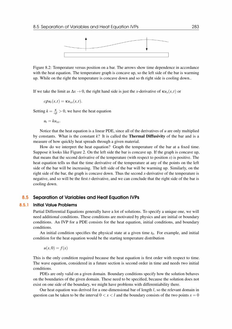
8.5 Separation of Variables and Heat Equation IVPs 283
Figure 8.2: Temperature versus position on a bar. The arrows show time dependence in accordancewith the heat equation. The temperature graph is concave up, so the left side of the bar is warmingup. While on the right the temperature is concave down and so th right side is cooling down..
If we take the limit as ∆x→ 0, the right hand side is just the x-derivative of κux(x, t) or
cρut(x, t) = κuxx(x, t).
Setting k = κ
cρ> 0, we have the heat equation
ut = kuxx.
Notice that the heat equation is a linear PDE, since all of the derivatives of u are only multipliedby constants. What is the constant k? It is called the Thermal Diffusivity of the bar and is ameasure of how quickly heat spreads through a given material.
How do we interpret the heat equation? Graph the temperature of the bar at a fixed time.Suppose it looks like Figure 2. On the left side the bar is concave up. If the graph is concave up,that means that the second derivative of the temperature (with respect to position x) is positive. Theheat equation tells us that the time derivative of the temperature at any of the points on the leftside of the bar will be increasing. The left side of the bar will be warming up. Similarly, on theright side of the bar, the graph is concave down. Thus the second x-derivative of the temperature isnegative, and so will be the first t-derivative, and we can conclude that the right side of the bar iscooling down.
8.5 Separation of Variables and Heat Equation IVPs
8.5.1 Initial Value ProblemsPartial Differential Equations generally have a lot of solutions. To specify a unique one, we willneed additional conditions. These conditions are motivated by physics and are initial or boundaryconditions. An IVP for a PDE consists for the heat equation, initial conditions, and boundaryconditions.
An initial condition specifies the physical state at a given time t0. For example, and initialcondition for the heat equation would be the starting temperature distribution
u(x,0) = f (x)
This is the only condition required because the heat equation is first order with respect to time.The wave equation, considered in a future section is second order in time and needs two initialconditions.
PDEs are only valid on a given domain. Boundary conditions specify how the solution behaveson the boundaries of the given domain. These need to be specified, because the solution does notexist on one side of the boundary, we might have problems with differentiability there.
Our heat equation was derived for a one-dimensional bar of length l, so the relevant domain inquestion can be taken to be the interval 0 < x < l and the boundary consists of the two points x = 0

284 Chapter 8. Partial Differential Equations
and x = l. We could have derived a two-dimensional heat equation, for example, in which case thedomain would be some region in the xy-plane with the boundary being some closed curve.
It will be clear from the physical description of the problem what the appropriate boundaryconditions are. We might know at the endpoints x = 0 and x = l, the temperature u(0, t) and u(l, t)are fixed. Boundary conditions that give the value of the solution are called Dirichlet BoundaryConditions. Or we might insulate the ends of the bar, meaning there should be no heat flowout of the boundary. This would yield the boundary conditions ux(0, t) = ux(l, t) = 0. If theboundary conditions specify the derivative at the boundary, they are called Neumann Conditions.If the boundary conditions specify that we have one insulated end and at the other we control thetemperature. This is an example of a Mixed Boundary Condition.
As we have seen, changing boundary conditions can significantly change the solution. Initially,we will work with homogeneous Dirichlet conditions u(0, t) = u(l, t) = 0, giving us the followinginitial value problem
(DE) : ut = kuxx (8.33)
(BC) : u(0, t) = u(l, t) = 0 (8.34)
(IC) : u(x,0) = f (x) (8.35)
After we have seen the general method, we will see what happens with homogeneous Neumannconditions. We will discuss nonhomogeneous equations later.
8.5.2 Separation of VariablesAbove we have derived the heat equation for the bar of length L. Suppose we have an initial valueproblem such as Equation (8.33)-(8.35). How should we proceed? We want to try to build a generalsolution out of smaller solutions which are easier to find.
We start by assuming we have a separated solution, where
u(x, t) = X(x)T (t).
Our solution is the product of a function that depends only on x and a function that depends only ont. We can then try to write down an equation depending only on x and another solution dependingonly on t before using our knowledge of ODEs to try and solve them.
It should be noted that this is a very special situation and will not occur in general. Even whenwe can use it sometimes it is hard to move beyond the first step. However, it works for all equationswe will be considering in this class, and is a good starting point.
How does this method work? Plug the separated solution into the heat equation.
∂
∂ t[X(x)T (t)] = k
∂ 2
∂x2 [X(x)T (t)] (8.36)
X(x)T ′(t) = kX ′′(x)T (t) (8.37)
Now notice that we can move everything depending on x to one side and everything depending on tto the other.
T ′(t)kT (t)
=X ′′(x)X(x)
This equation should says that both sides are equal for any x or t we choose. Thus they both mustbe equal to a constant. Since if what they equal depended on x or t both sides would not be equalfor all x and t. So
T ′(t)kT (t)
=X ′′(x)X(x)
=−λ

8.5 Separation of Variables and Heat Equation IVPs 285
We have written the minus sign for convenience. It will turn out that λ > 0.The equation above contains a pair of separate ordinary differential equations
X ′′+λX = 0 (8.38)
T ′+λkT = 0. (8.39)
Notice that our boundary conditions becomes X(0) = 0 and X(l) = 0. Now the second equationcan easily be solved, since we have T ′ =−λkT , so that
T (t) = Ae−λkt .
The first equation gives a boundary value problem
X ′′+λX = 0 X(0) = 0 X(l) = 0
This should look familiar. The is the basic eigenfunction problem studied in section 10.1. As inthat example, it turns out our eigenvalues have to be positive. Let λ = µ2 for µ > 0, our generalsolution is
X(x) = Bcos(µx)+C sin(µx).
The first boundary condition says B = 0. The second condition says that X(l) =C sin(µl) = 0. Toavoid only having the trivial solution, we must have µl = nπ . In other words,
λn =(nπ
l
)2 and Xn(x) = sin(nπx
l
)for n = 1,2,3, ...
So we end up having found infinitely many solutions to our boundary value problem, one foreach positive integer n. They are
un(x, t) = Ane−(nπ
l )2kt sin(nπx
l).
The heat equation is linear and homogeneous. As such, the Principle of Superposition still holds.So a linear combination of solutions is again a solution. So any function of the form
u(x, t) =N
∑n=0
Ane−(nπ
l )2kt sin(nπx
l) (8.40)
is also a solution to our problem.Notice we have not used our initial condition yet. We have
f (x) = u(x,0) =N
∑n=0
An sin(nπx
l).
So if our initial condition has this form, the result of superposition Equation (8.40) is in a goodform to use the IC. The coefficients An just being the associated coefficients from f (x).
Example 8.7 Find the solutions to the following heat equation problem on a rod of length 2.
ut = uxx (8.41)
u(0, t) = u(2, t) = 0 (8.42)
u(x,0) = sin(3πx
2)−5sin(3πx) (8.43)

286 Chapter 8. Partial Differential Equations
In this problem, we have k = 1. Now we know that our solution will have the form likeEquation (8.40), since our initial condition is just the difference of two sine functions. We just needto figure out which terms are represented and what the coefficients An are.
Our initial condition is
f (x) = sin(3πx
2)−5sin(3πx)
Looking at (8.40) with l = 2, we can see that the first term corresponds to n = 3 and the secondn = 6, and there are no other terms. Thus we have A3 = 1 and A6 =−5, and all other An = 0. Oursolution is then
u(x, t) = e−(9π2
4 )t sin(3πx
2)−5e(−9π2)t sin(3πx).
There is no reason to suppose that our initial distribution is a finite sum of sine functions.Physically, such situations are special. What do we do if we have a more general initial temperaturedistribution?
Let’s consider what happens if we take an infinite sum of our separated solutions. Then oursolution is
u(x, t) =∞
∑n=0
Ane−(nπ
l )2kt sin(nπx
l).
Now the initial condition gives
f (x) =∞
∑n=0
An sin(nπx
l).
This idea is due to the French Mathematician Joseph Fourier and is called the Fourier Sine Seriesfor f (x).
There are several important questions that arise. Why should we believe that our initial conditionf (x) ought to be able to be written as an infinite sum of sines? why should we believe that such asum would converge to anything?
8.5.3 Neumann Boundary ConditionsNow let’s consider a heat equation problem with homogeneous Neumann conditions
(DE) : ut = uxx (8.44)
(BC) : ux(0, t) = ux(l, t) = 0 (8.45)
(IC) : u(x,0) = f (x) (8.46)
We will start by again supposing that our solution to Equation (8.44) is separable, so we haveu(x, t) = X(x)T (t) and we obtain a pair of ODEs, which are the same as before
X ′′+λX = 0 (8.47)
T ′+λkT = 0. (8.48)
The solution to the first equation is still
T (t) = Ae−λkt

8.6 Heat Equation Problems 287
Now we need to determine the boundary conditions for the second equation. Our boundaryconditions are ux(0, t) and ux(l, t). Thus they are conditions for X ′(0) and X ′(l), since the t-derivative is not controlled at all. So we have the boundary value problem
X ′′+λX = 0 X ′(0) = 0 X ′(l) = 0.
Along the lines of the analogous computation last lecture, this has eigenvalues and eigenfunctions
λn =(nπ
l
)2 (8.49)
yn(x) = cos(nπx
l
)(8.50)
for n = 0,1,2, ... So the individual solutions to Equation (8.44) have the form
u(x, t) = Ane(nπ
l )2kt cos(nπx
l
).
Taking finite linear combinations of these work similarly to the Dirichlet case (and is the solutionto Equation (8.44) when f (x) is a finite linear combination of constants and cosines, but in generalwe are interested in knowing when we can take infinite sums, i.e.
u(x, t) =12
A0 +∞
∑n=1
Ane−(nπ
l )2kt cos(nπx
l)
Notice how we wrote the n = 0 case, as 12 A0. The reason will be clear when talking about Fourier
Series. The initial conditions means we need
f (x) =12
A0 +∞
∑n=1
An cos(nπx
l).
An expression of the form above is called the Fourier Cosine Series of f (x).
8.5.4 Other Boundary ConditionsIt is also possible for certain boundary conditions to require the "full" Fourier Series of the initialdata, this is an expression of the form
f (x) =12
A0 +∞
∑n=1
(An cos
(nπxl
)+Bn sin
(nπxl
)).
but in most cases we will work with Dirichlet or Neumann conditions. However, in the process oflearning about Fourier sine and cosine series, we will also learn how to compute the full Fourierseries of a function.
8.6 Heat Equation ProblemsIn the previous lecture on the Heat Equation we saw that the product solutions to the heat equationwith homogeneous Dirichlet boundary conditions problem
ut = kuxx (8.51)
u(0, t) = u(l, t) = 0 (8.52)
u(x,0) = f (x) (8.53)
had the form
un(x, t) = Bne−(nπ
l )kt sin(nπx
l
)n = 1,2,3, ...

288 Chapter 8. Partial Differential Equations
Taking linear combinations of these (over each n) gives a general solution to the above problem.
u(x, t) =∞
∑n=1
Bne−(nπ
l )kt sin(nπx
l
)(8.54)
Setting t = 0, this implies that we must have
f (x) =∞
∑n=1
Bn sin(nπx
l
)In other words, the coefficients in the general solution for the given initial condition are the FourierSine coefficients of f (x) on (0, l), which are given by
Bn =2l
∫ l
0f (x)sin
(nπxl
)dx.
We also, saw that if we instead have a problem with homogeneous Neumann boundary condi-tions
ut = kuxx 0 < x < l, t > 0 (8.55)
ux(0, t) = ux(l, t) = 0 (8.56)
u(0, t) = f (x) (8.57)
the product solutions had the form
un(x, t) = Ane−(nπ
l )2kt cos(nπx
l
)n = 1,2,3, ...
and the general solution has the form
u(x, t) =12
A0 +∞
∑n=1
Ane−(nπ
l )2kt cos(nπx
l
). (8.58)
With t = 0 this means that the initial condition must satisfy
f (x) =12
A0 +∞
∑n=1
An cos(nπx
l
).
and so the coefficients for a particular initial condition are the Fourier Cosine coefficients of f (x),given by
An =2l
∫ l
0f (x)cos
(nπxl
)dx.
One way to think about this difference is that given the initial data u(x,0) = f (x), the Dirichletconditions specify the odd extension of f (x) as the desired periodic solution, while the Neumannconditions specify the even extension. This should make sense since odd functions must havef (0) = 0, while even functions must have f ′(0) = 0.
So to solve a homogeneous heat equation problem, we begin by identifying the type of boundaryconditions we have. If we have Dirichlet conditions, we know our solution will have the form ofEquation (8.54). All we then have to do is compute the Fourier Sine coefficients of f (x). Similarly,if we have Neumann conditions, we know the solution has the form of Equation (8.114) and wehave to compute the Fourier Cosine coefficients of f (x).

8.6 Heat Equation Problems 289
R Observe that for any homogeneous Dirichlet problem, the temperature distribution (8.54)will go to 0 as t → ∞. This should make sense because these boundary conditions have aphysical interpretation where we keep the ends of our rod at freezing temperature withoutregulating the heat flow in and out of the endpoints. As a result, if the interior of the rod isinitially above freezing, that heat will radiate towards the endpoints and into our reservoirs atthe endpoints. On the other hand, if the interior of the rod is below freezing, heat will comefrom the reservoirs at the endpoints and warm it up until the temperature is uniform.
For the Neumann problem, the temperature distribution (8.114) will converge to 12 A0. Again,
this should make sense because these boundary conditions correspond to a situation wherewe have insulated ends, since we are preventing any heat from escaping the bar. Thus all heatenergy will move around inside the rod until the temperature is uniform.
8.6.1 Examples Example 8.8 Solve the initial value problem
ut = 3uxx 0 < x < 2, t > 0 (8.59)
u(0, t) = u(2, t) = 0 (8.60)
u(x,0) = 20. (8.61)
This problem has homogeneous Dirichlet conditions, so by (8.54) our general solution is
u(x, t) =∞
∑n=1
Bne−3( nπ
2 )2t sin(nπx
2).
The coefficients for the particular solution are the Fourier Sine coefficients of u(x,0) = 20, so wehave
Bn =22
∫ 2
020sin(
nπx2
)dx (8.62)
= [− 40nπ
cos(nπx
2)]20 (8.63)
= − 40nπ
(cos(nπ)− cos(0)) (8.64)
=40nπ
(1+(−1)n+1) (8.65)
and the solution to the problem is
u(x, t) =40π
∞
∑n=1
1+(−1)n+1
ne−
3n2π24 t sin(
nπx2
).
Example 8.9 Solve the initial value problem
ut = 3uxx 0 < x < 2, t > 0 (8.66)
ux(0, t) = ux(2, t) = 0 (8.67)
u(x,0) = 3x. (8.68)
This problem has homogeneous Neumann conditions, so by (8.114) our general solution is
u(x, t) =12
A0 +∞
∑n=1
Ane−3( nπ
2 )2t cos(nπx
2).

290 Chapter 8. Partial Differential Equations
The coefficients for the particular solution are the Fourier Cosine coefficients of u(x,0) = 3x, so wehave
A0 =22
∫ 2
03xdx = 6 (8.69)
An =22
∫ 2
03xcos(
nπx2
)dx (8.70)
= [− 6xnπ
cos(nπx
2)+
12n2π2 sin(
nπx2
)]20 (8.71)
= − 12nπ
cos(nπ) (8.72)
=12nπ
(−1)n+1 (8.73)
and the solution to the problem is
u(x, t) =32+
12π
∞
∑n=1
(−1)n+1
ne−
3n2π24 t cos(
nπx2
).
Example 8.10 Solve the initial value problem
ut = 4uxx 0 < x < 2π, t > 0 (8.74)
u(0, t) = u(2π, t) = 0 (8.75)
u(x,0) =
1 0 < x < π
x π < x < 2π. (8.76)
This problem has homogeneous Dirichlet conditions, so our general solution is
u(x, t) =∞
∑n=1
Bne−n2t sin(nx2).
The coefficients for the particular solution are the Fourier Sine coefficients of u(x,0), so we have
Bn =2
2π
(∫π
0sin(
nx2)dx+
∫ 2π
π
xsin(nx2)dx)
(8.77)
= − 2nπ
cos(nx2)|π0 −
2xnπ
cos(nx2)|2π
π +4
n2πsin(
nx2)|2π
π (8.78)
= − 2nπ
(cos(nx2)− cos(0))− 4
ncos(nπ)+
2n
cos(nπ
2)− 4
n2πsin(
nπ
2) (8.79)
= − 2nπ
(cos(nπ
2)−1)+
4n(−1)n+1 +
2n
cos(nπ
2)− 4
n2πsin(
nπ
2) (8.80)
=2n
(− 1
π(cos(
nπ
2)−1)+2(−1)n+1 cos(
nπ
2)− 2
nπsin(
nπ
2)
)(8.81)
and the solution to the problem is
u(x, t) = 2∞
∑n=1
1n
(− 1
π(cos(
nπ
2)−1)+2(−1)n+1 cos(
nπ
2)− 2
nπsin(
nπ
2)
)e−n2t sin(
nx2).

8.7 Other Boundary Conditions 291
8.7 Other Boundary ConditionsSo far, we have used the technique of separation of variables to produce solutions to the heatequation
ut = kuxx
on 0 < x < l with either homogeneous Dirichlet boundary conditions [u(0, t) = u(l, t) = 0] orhomogeneous Neumann boundary conditions [ux(0, t) = ux(l, t) = 0]. What about for some otherphysically relevant boundary conditions?
8.7.1 Mixed Homogeneous Boundary ConditionsWe could have the following boundary conditions
u(0, t) = ux(l, t) = 0
Physically, this might correspond to keeping the end of the rod where x = 0 in a bowl of ice water,while the other end is insulated.
Use Separation of Variables. Let u(x, t) = X(x)T (t), and we get the pair of ODEs
T ′ = −kλT (8.82)
X ′′ = −λX . (8.83)
Thus
T (t) = Be−kλ t .
We now have a boundary value problem for X to deal with, where the boundary conditions areX(0) = X ′(l) = 0. There are only positive eigenvalues, which are given by
λn =
((2n−1)π
2l
)2
and their associated eigenfunctions are
Xn(x) = sin((2n−1)πx
2l).
The separated solutions are then given by
un(x, t) = Bne−((2n−1)π
2l )2kt sin((2n−1)πx
2l
)and the general solution is
u(x, t) =∞
∑n=1
Bne−((2n−1)π
2l )2kt sin((2n−1)πx
2l
). (8.84)
with an initial condition u(x,0) = f (x), we have that
f (x) =∞
∑n=1
Bn sin((2n−1)πx
2l
).
This is an example of a specialized sort of Fourier Series, the coefficients are given by
Bn =2l
∫ l
0f (x)sin
((2n−1)πx2l
)dx.

292 Chapter 8. Partial Differential Equations
R The convergence for a series like the one above is different than that of our standard FourierSine or Cosine series, which converge to the periodic extension of the odd or even extensionsof the original function, respectively. Notice that the terms in the sum above are periodic withperiod 4l (as opposed to the 2l-periodic series we have seen before). In this case, we need tofirst extend our function f (x), given on (0, l), to a function on (0,2l) symmetric around x = l.Then, as our terms are all sines, the convergence on (−2l,2l) will be to the odd extension ofthis extended function, and the periodic extension of this will be what the series converges toon the entire real line.
Example 8.11 Solve the following heat equation problem
ut = 25uxx (8.85)
u(0, t) = 0 ux(10, t) = 0 (8.86)
u(x,0) = 5. (8.87)
By (8.84) our general solution is
u(x, t) =∞
∑n=1
Bne−25( (2n−1)π20 )2t sin
((2n−1)πx20
).
The coefficients for the particular solution are given by
Bn =210
∫ 10
05sin
((2n−1)πx20
)dx (8.88)
= − 10(2n−1)π
cos((2n−1)πx
20)|100 (8.89)
= − 10(2n−1)π
(cos(
(2n−1)π2
)− cos(0))
(8.90)
=10
(2n−1)π. (8.91)
and the solution to the problem is
u(x, t) =10π
∞
∑n=1
1(2n−1)
e−(2n−1)2π2
16 t sin((2n−1)πx
20).
8.7.2 Nonhomogeneous Dirichlet ConditionsThe next type of boundary conditions we will look at are Dirichlet conditions, which fix the value ofu at the endpoints x = 0 and x = l. For the heat equation, this corresponds to fixing the temperatureat the ends of the rod. We have already looked at homogeneous conditions where the ends of therod had fixed temperature 0. Now consider the nonhomogeneous Dirichlet conditions
u(0, t) = T1, u(l, t) = T2
This problem is slightly more difficult than the homogeneous Dirichlet condition problem wehave studied. Recall that for separation of variables to work, the differential equations and theboundary conditions must be homogeneous. When we have nonhomogeneous conditions we needto try to split the problem into one involving homogeneous conditions, which we know how tosolve, and another dealing with the nonhomogeneity.
R We used a similar approach when we applied the method of Undetermined Coefficients tononhomogeneous linear ordinary differential equations.

8.7 Other Boundary Conditions 293
How can we separate the core homogeneous problem from what is causing the inhomogeneity?Consider what happens as t → ∞. We should expect that, since we fix the temperatures at theendpoints and allow free heat flux at the boundary, at some point the temperature will stabilize andwe will be at equilibrium. Such a temperature distribution would clearly not depend on time, andwe can write
limt→∞
u(x, t) = v(x)
Notice that v(x) must still satisfy the boundary conditions and the heat equation, but we shouldnot expect it to satisfy the initial conditions (since for large t we are far from where we initiallystarted). A solution such as v(x) which does not depend on t is called a steady-state or equilibriumsolution.
For a steady-state solution the boundary value problem becomes
0 = kv′′ v(0) = T1 v(l) = T2.
It is easy to see that solutions to this second order differential equation are
v(x) = c1x+ c2
and applying the boundary conditions, we have
v(x) = T1 +T2−T1
lx.
Now, let
w(x, t) = u(x, t)− v(x)
so that
u(x, t) = w(x, t)+ v(x).
This function w(x, t) represents the transient part of u(x, t) (since v(x) is the equilibrium part).Taking derivatives we have
ut = wt + vt = wt and uxx = wxx + vxx = wxx.
Here we use the fact that v(x) is independent of t and must satisfy the differential equation. Also,using the equilibrium equation v′′ = vxx = 0.
Thus w(x, t) must satisfy the heat equation, as the relevant derivatives of it are identical to thoseof u(x, t), which is known to satisfy the equation. What are the boundary and initial conditions?
w(0, t) = u(0, t)− v(0) = T1−T1 = 0 (8.92)
w(l, t) = u(l, t)− v(l) = T2−T2 = 0 (8.93)
w(x,0) = u(x,0)− v(x) = f (x)− v(x) (8.94)
where f (x) = u(x,0) is the given initial condition for the nonhomogeneous problem. Now, eventhough our initial condition is slightly messier, we now have homogeneous boundary conditions,since w(x, t) must solve the problem
wt = kwxx (8.95)
w(0, t) = w(l, t) = 0 (8.96)
w(x,0) = f (x)− v(x) (8.97)

294 Chapter 8. Partial Differential Equations
This is just a homogeneous Dirichlet problem. We know the general solution is
w(x, t) =∞
∑n=1
Bne−(nπ
l )2kt sin(nπx
l).
where the coefficients are given by
Bn =2l
∫ l
0( f (x)− v(x))sin(
nπxl
)dx.
Notice that limt→∞ w(x, t) = 0, so that w(x, t) is transient.Thus, the solution to the nonhomogeneous Dirichlet problem
ut = kuxx (8.98)
u(0, t) = T1, u(l, t) = T2 (8.99)
u(x,0) = f (x) (8.100)
is u(x, t) = w(x, t)+ v(x), or
u(x, t) =∞
∑n=1
Bne−(nπ
l )2lt sin(nπx
l
)+T1 +
T2−T1
lx
with coefficients
Bn =2l
∫ l
0( f (x)−T1−
T2−T1
lx)sin
(nπxl
)dx.
R Do not memorize the formulas but remember what problem w(x, t) has to solve and that thefinal solution is u(x, t) = v(x)+w(x, t). For v(x), it is not a hard formula, but if one is notsure of it, remember vxx = 0 and it has the same boundary conditions as u(x, t). This willrecover it.
Example 8.12 Solve the following heat equation problem
ut = 3uxx (8.101)
u(0, t) = 20, u(40, t) = 100 (8.102)
u(x,0) = 40−3x (8.103)
We start by writing
u(x, t) = v(x)+w(x, t)
where v(x) = 20+2x. Then w(x, t) must satisfy the problem
wt = 3wxx (8.104)
w(0, t) = w(40, t) = 0 (8.105)
w(x,0) = 40−3x− (20+2x) = 20− x (8.106)
This is a homogeneous Dirichlet problem, so the general solution for w(x, t) will be
w(x, t) =∞
∑n=1
e−3( nπ
40 )2t sin(
nπx40
).

8.8 The Schrödinger Equation 295
The coefficients are given by
Bn =240
∫ 40
0(20− x)sin
(nπx40)dx (8.107)
=120
[−40(20− x)nπ
cos(nπx
40)− 1600
n2π2 sin(nπx
40)]40
0 (8.108)
=120
(800nπ
cos(nπ)+800nπ
cos(0))
(8.109)
=40nπ
((−1)n +1). (8.110)
So the solution is
u(x, t) = 20+2x+40π
∞
∑n=1
(−1)n +1n
e−3n2π21600 t sin
(nπx40).
8.7.3 Other Boundary ConditionsThere are many other boundary conditions one could use, most of which have a physical interpreta-tion. For example the boundary conditions
u(0, t)+ux(0, t) = 0 u(l, t)+ux(l, t) = 0
say that the heat flux at the end points should be proportional to the temperature. We could alsohave had nonhomogeneous Neumann conditions
ux(0, t) = F1 ux(l, t) = F2
which would specify allowing a certain heat flux at the boundaries. These conditions are notnecessarily well suited for the method of separation of variables though and are left for futureclasses.
8.8 The Schrödinger EquationRecall the Schrödinger equation
− h2m
∆Ψ+V Ψ = ih∂
∂ tΨ. (8.111)
To approach this problem we begin by separating variables by assuming Ψ = ψ(x,y,z)T (t). Substi-tution into (8.111) gives
− h2m
1ψ
∆ψ +V = ih1T
dTdt
= E
where E is the separation constant (E is the energy of the particle in quantum mechanics). Integrat-ing the time equation in T gives
ih1T
dTdt
= E ⇒ T (t) = e−iEt/h.
and the space equation (Time-independent Schrödinger equation gives (after multiplication by ψ)
− h2m
∆ψ +V ψ = Eψ

296 Chapter 8. Partial Differential Equations
We will only consider the simplest situation here of a 1D problem with V = 0
− h2m
d2ψ
dx2 = Eψ ⇔ d2ψ
dx2 +2mEh2 ψ = 0.
The last equation is the Helmholtz equation with k2 = 2mEh2 . Thus, the solutions are
Ψ = ψ(x)T (t) = sin(kx)e−iEt/h,cos(kx)e−iEt/h.
Example 8.13 The “particle in a box" problem in quantum mechanics requires the solution ofthe Schrödinger equation with V = 0 on (0, `) and Ψ = 0 at the endpoints x = 0, ` for all t. TheDirichlet BCs require only the solutions with sine. The basis functions for this problem are theeigenfunctions
Ψn = sin(nπx
`
)r−iEnt/h
and the general solution is a linear combination of these solutions
Ψ(x, t) =∞
∑n=1
bn sin(nπx
`
)r−iEnt/h
8.9 Wave Equations and the Vibrating String8.9.1 Derivation of the Wave Equation
Consider a completely flexible string of length l and constant density ρ . We will assume that thestring will only undergo relatively small vertical vibrations, so that points do not move from sideto side. An example might be a plucked guitar string. Thus we can let u(x, t) be its displacementfrom equilibrium at time t. The assumption of complete flexibility means that the tension force istangent to the string, and the string itself provides no resistance to bending. This means the tensionforce only depends on the slope of the string.
Take a small piece of string going from x to x+∆x. Let Θ(x, t) be the angle from the horizontalof the string. Our goal is to use Newton’s Second Law F = ma to describe the motion. What forcesare acting on this piece of string?(a) Tension pulling to the right, which has magnitude T (x+∆x, t) and acts at an angle of Θ(x+∆x, t)from the horizontal.(b) Tension pulling to the left, which has magnitude T (x, t) and acts at an angle of Θ(x, t) from thehorizontal.(c) Any external forces, which we denote by F(x, t).Initially, we will assume that F(x, t) = 0. The length of the string is essentially
√(∆x)2 +(∆u)2,
so the vertical component of Newton’s Law says that
ρ
√(∆x)2 +(∆u)2utt(x, t) = T (x+∆x, t)sin(Θ(x+∆x, t))−T (x, t)sin(Θ(x, t)). (8.112)
Dividing by ∆x and taking the limit as ∆x→ 0, we get
ρ
√1+(ux)2utt(x, t) =
∂
∂x[T (x, t)sin(Θ(x, t))]. (8.113)
We assumed our vibrations were relatively small. This means that Θ(x, t) is very close to zero. As aresult, sin(Θ(x, t))≡ tan(Θ(x, t)). Moreover, tan(Θ(x, t)) is just the slope of the string ux(x, t). Weconclude, since Θ(x, t) is small, that ux(x, t) is also very small. The above equation becomes
ρutt(x, t) = (T (x, t)ux(x, t))x. (8.114)

8.9 Wave Equations and the Vibrating String 297
We have not used the horizontal component of Newton’s Law yet. Since we assume there are onlyvertical vibrations, our tiny piece of string can only move vertically. Thus the net horizontal forceis zero.
T (x+∆x, t)cos(Θ(x+∆x, t))−T (x, t)cos(Θ(x, t)) = 0. (8.115)
Dividing by ∆x and taking the limit as ∆x→ ∞ yields
∂
∂x[T (x, t)cos(Θ(x, t))] = 0. (8.116)
Since Θ(x, t) is very close to zero, cos(Θ(x, t)) is close to one. thus we have that ∂T∂x (x, t) is close
to zero. So T (x, t) is constant along the string, and independent of x. We will also assume that T isindependent of t. Then Equation (8.114) becomes the one-dimensional wave equation
utt = c2uxx (8.117)
where c2 = Tρ
.
8.9.2 The Homogeneous Dirichlet ProblemNow that we have derived the wave equation, we can use Separation of Variables to obtain basicsolutions. We will consider homogeneous Dirichlet conditions, but if we had homogeneousNeumann conditions the same techniques would give us a solution. The wave equation is secondorder in t, unlike the heat equation which was first order in t. We will need to initial conditions inorder to obtain a solution, one for the initial displacement and the other for the initial speed.
The relevant wave equation problem we will study is
utt = c2uxx (8.118)
u(0, t) = u(l, t) = 0 (8.119)
u(x,0) = f (x), ut(x,0) = g(x) (8.120)
The physical interpretation of the boundary conditions is that the ends of the string are fixed inplace. They might be attached to guitar pegs.
We start by assuming our solution has the form
u(x, t) = X(x)T (t). (8.121)
Plugging this into the equation gives
T ′′(t)X(x) = c2T (t)X ′′(x). (8.122)
Separating variables, we have
X ′′
X=
T ′′
c2T=−λ (8.123)
where λ is a constant. This gives a pair of ODEs
T ′′+ c2λT = 0 (8.124)
X ′′+λX = 0. (8.125)
The boundary conditions transform into
u(0, t) = X(0)T (t) = 0 ⇒ X(0) = 0 (8.126)
u(l, t) = X(l)T (t) = 0 ⇒ X(l) = 0. (8.127)
298 Chapter 8. Partial Differential Equations
This is the same boundary value problem that we saw for the heat equation and thus the eigenvaluesand eigenfunctions are
λn =(nπ
l
)2 (8.128)
Xn(x) = sin(nπx
l
)(8.129)
for n = 1,2, ... The first ODE (8.124) is then
T ′′+(cnπ
l
)2T = 0, (8.130)
and since the coefficient of T is clearly positive this has a general solution
Tn(t) = An cos(nπct
l
)+Bn sin
(nπctl
). (8.131)
There is no reason to think either of these are zero, so we end up with separated solutions
un(x, t) =[
An cos(nπct
l)+Bn sin(
nπctl
)
]sin(
nπxl
) (8.132)
and the general solution is
u(x, t) =∞
∑n=1
[An cos(
nπctl
)+Bn sin(nπct
l)
]sin(
nπxl
). (8.133)
We can directly apply our first initial condition, but to apply the second we will need to differentiatewith respect to t. This gives us
ut(x, t) =∞
∑n=1
[−nπc
lAn sin(
nπctl
)+nπc
lBn cos(
nπctl
)
]sin(
nπxl
) (8.134)
Plugging in the initial condition then yields the pair of equations
u(x,0) = f (x) =∞
∑n=1
An sin(nπx
l) (8.135)
ut(x,0) = g(x) =∞
∑n=1
nπcl
Bn sin(nπx
l). (8.136)
These are both Fourier Sine series. The first is directly the Fourier Since series for f (x) on (0, l).The second equation is the Fourier Sine series for g(x) on (0, l) with a slightly messy coefficient.The Euler-Fourier formulas then tell us that
An =2l
∫ l
0f (x)sin(
nπxl
)dx (8.137)
nπcl
Bn =2l
∫ l
0g(x)sin(
nπxl
)dx (8.138)
An =2l
∫ l
0f (x)sin(
nπxl
)dx (8.139)
Bn =2
nπc
∫ l
0g(x)sin(
nπxl
)dx. (8.140)

8.9 Wave Equations and the Vibrating String 299
8.9.3 Examples Example 8.14 Find the solution (displacement u(x, t)) for the problem of an elastic string oflength L whose ends are held fixed. The string has no initial velocity (ut(x,0) = 0) from an initialposition
u(x,0) = f (x) =
4xL 0≤ x≤ L
4
1 L4 < x < 3L
44(L−x)
L3L4 ≤ x≤ L
(8.141)
By the formulas above we see if we separate variables we have the following equation for T
T ′′+(cnπ
L)2T = 0 (8.142)
with the general solution
Tn(t) = An cos(nπct
L)+Bn sin(
nπctL
). (8.143)
since the initial speed is zero, we find T ′(0) = 0 and thus Bn = 0. Therefore the general solution is
u(x, t) =∞
∑n=1
An cos(nπct
L)sin(
nπxL
). (8.144)
where the coefficients are the Fourier Sine coefficients of f (x). So
An =2L
∫ L
0f (x)sin(
nπxL
)dx (8.145)
=2L
[∫ L/4
0
4xL
sin(nπx
L)dx+
∫ 3L/4
L/4sin(
nπxL
)dx+∫ L
3L/4
4L−4xL
sin(nπx
L)dx]
(8.146)
= 8sin(nπ
4 )+ sin(3nπ
4 )
n2π2 (8.147)
Thus the displacement of the string will be
u(x, t) =8
π2
∞
∑n=1
sin(nπ
4 )+ sin(3nπ
4 )
π2 cos(nπct
L)sin(
nπxL
). (8.148)
Example 8.15 Find the solution (displacement u(x, t)) for the problem of an elastic string oflength L whose ends are held fixed. The string has no initial velocity (ut(x,0) = 0) from an initialposition
u(x,0) = f (x) =8x(L− x)2
L3 (8.149)
By the formulas above we see if we separate variables we have the following equation for T
T ′′+(cnπ
L)2T = 0 (8.150)
with the general solution
Tn(t) = An cos(nπct
L)+Bn sin(
nπctL
). (8.151)

300 Chapter 8. Partial Differential Equations
since the initial speed is zero, we find T ′(0) = 0 and thus Bn = 0. Therefore the general solution is
u(x, t) =∞
∑n=1
An cos(nπct
L)sin(
nπxL
). (8.152)
where the coefficients are the Fourier Sine coefficients of f (x). So
An =2L
∫ L
0f (x)sin(
nπxL
)dx (8.153)
=2L
∫ L
0
8x(L− x)2
L3 sin(nπx
L)dx (8.154)
= 322+ cos(nπ)
n3π3 Integrate By Parts (8.155)
Thus the displacement of the string will be
u(x, t) =32π3
∞
∑n=1
2+ cos(nπ)
n3 cos(nπct
L)sin(
nπxL
). (8.156)
8.9.4 D’Alembert’s Solution of the Wave Equation, CharacteristicsAnother approach to solving the wave equation
∂ 2u∂ t2 = c2 ∂ 2u
∂x2 (8.157)
can be seen by transforming the equation. Introduce new independent variables:
v = x+ ct, w = x− ct (8.158)
We can now think of u as a function of v,w instead of x, t. Now compute the appropriate partialderivatives of u using the chain rule
∂u∂x
=∂u∂v
∂v∂x
+∂u∂w
∂w∂x
= uv +u+w.
∂ 2u∂x2 = (uv +uw)x = (uv +uw)vvx +(uv +uw)wwx = uvv +2uvw +uww
∂ 2u∂ t2 = c2(uvv−2uvw +uww).
Inserting these into the wave equation gives uvw = 0. Solve using two successive integrations, firstwith respect to w and then with respect to v giving
∂u∂v
= h(v), u(v,w) =∫
h(v)dv+ψ(w) = φ(v)+ψ(w).
Thus, replacing v and w by their definitions
u(x, t) = φ(x+ ct)+ψ(x− ct) (8.159)
This is known as d’Alembert’s solution. In general given initial conditions u(x,0) = f (x) andut(x,0) = g(x), d’Alembert’s solution becomes
u(x, t) =12[ f (x+ ct)+ f (x− ct)]+
12c
∫ x+ct
x−ctg(s)ds. (8.160)

8.9 Wave Equations and the Vibrating String 301
R The idea of d’Alembert’s solution is just a special case of the method of characteristics.This concerns PDEs of the form
Auxx +2Buxy +Cuyy = F(x,y,u,ux,uy). (8.161)
PDEs have three general types defined by the coefficients A,B,C and the discriminant AC−B2
Figure 8.3: Three general types of PDEs, (from Kreysig Adv. Engineering Math).


Index
complex plane, 9complex variables, 9
imaginary part, 9
real part, 9