Embed Size (px)
Citation preview

Mathematical Logic and its Application to
Computer Science
Lecture Notes
Eitan Farchi
Yochai Ben-Chaim
March 3, 2010
1

Contents
1 Introduction 9
1.1 The Knaves and the Knights . . . . . . . . . . . . . . . . . . . 9
1.2 Inductive Definitions of Sets . . . . . . . . . . . . . . . . . . . 10
1.2.1 Initial Definition . . . . . . . . . . . . . . . . . . . . . 10
1.2.2 MI/MU Example . . . . . . . . . . . . . . . . . . . . . 10
1.2.3 A Formal Definition . . . . . . . . . . . . . . . . . . . 13
1.2.4 Bottom-Up Definition . . . . . . . . . . . . . . . . . . 14
1.2.5 Induction Proof Principle . . . . . . . . . . . . . . . . 16
1.3 Propositional Calculus . . . . . . . . . . . . . . . . . . . . . . 17
1.3.1 Syntax . . . . . . . . . . . . . . . . . . . . . . . . . . . 17
1.3.2 Axiom . . . . . . . . . . . . . . . . . . . . . . . . . . . 19
1.4 Ruling Function from the Talmud . . . . . . . . . . . . . . . . 20
I Lecture Transcripts 23
2 Lecture - Inductive Sets 23
2.1 Definition . . . . . . . . . . . . . . . . . . . . . . . . . . . . . 23
2.1.1 Generic Example 1 . . . . . . . . . . . . . . . . . . . . 24
2.1.2 Generic Example 2 . . . . . . . . . . . . . . . . . . . . 25
2.1.3 Vertex Example . . . . . . . . . . . . . . . . . . . . . . 25
2.1.4 Using Inductive Sets in Defining Program Behavior . . 27
2.1.5 MI/MU Example . . . . . . . . . . . . . . . . . . . . . 28
2.1.6 Operative and Declarative Definitions . . . . . . . . . . 35
2.1.7 Inductive Sets in Computer Science . . . . . . . . . . . 36
2

3 Lecture - Inductive Sets Continued 42
3.1 Propositional Calculus . . . . . . . . . . . . . . . . . . . . . . 43
3.2 Induction on the Structure . . . . . . . . . . . . . . . . . . . . 44
3.3 Tautology . . . . . . . . . . . . . . . . . . . . . . . . . . . . . 44
3.3.1 Syntax . . . . . . . . . . . . . . . . . . . . . . . . . . . 45
3.3.2 Meaning of True Sentences . . . . . . . . . . . . . . . . 51
3.3.3 Tautologies . . . . . . . . . . . . . . . . . . . . . . . . 54
4 Lecture - Hierarchical Glossaries Example 57
4.1 Main Example . . . . . . . . . . . . . . . . . . . . . . . . . . . 60
4.2 Hierarchy of Dictionaries . . . . . . . . . . . . . . . . . . . . . 65
5 Lecture - Hierarchical Glossaries Example, Continued 67
5.1 Hierarchy of Rules for Glossary Design . . . . . . . . . . . . . 69
5.2 Introducing the Z Specification Language . . . . . . . . . . . . 71
5.3 Hierarchical Dictionaries Example, Continued . . . . . . . . . 74
5.4 Defining Adding a Word and its Definition to a Dictionary . . 75
5.5 Dictionary Example . . . . . . . . . . . . . . . . . . . . . . . . 77
5.6 Referred Sets . . . . . . . . . . . . . . . . . . . . . . . . . . . 77
5.7 Z Specification Language Basic Signs . . . . . . . . . . . . . . 78
6 Lecture - Formal Specification Languages 81
6.1 Formal Specification Language - Definition . . . . . . . . . . . 82
6.2 Ruling Function from the Talmud Revisited . . . . . . . . . . 86
7 Lecture - Communication Group Example 88
3

8 Lecture - Communication Group Example, Continued 94
9 Lecture - Communication Group Example, Continued 102
10 Lecture - Testing and Verification 108
10.1 Communication Group Example Summary . . . . . . . . . . . 108
10.2 Testing and Verification . . . . . . . . . . . . . . . . . . . . . 109
10.2.1 Model Checking . . . . . . . . . . . . . . . . . . . . . . 113
10.2.2 Functional Coverage . . . . . . . . . . . . . . . . . . . 115
10.2.3 Simulation . . . . . . . . . . . . . . . . . . . . . . . . . 117
11 Lecture - Abstraction 119
11.1 Generic Example 3 . . . . . . . . . . . . . . . . . . . . . . . . 119
12 Lecture - Relations and Functions 122
13 Lecture - Defining a Library Example 127
13.1 Defining A Function . . . . . . . . . . . . . . . . . . . . . . . 129
14 Lecture - Defining a Library Example, Continued 134
14.1 Defining a Library . . . . . . . . . . . . . . . . . . . . . . . . 134
14.2 File System Example . . . . . . . . . . . . . . . . . . . . . . . 137
14.3 Preparation for Final Exam . . . . . . . . . . . . . . . . . . . 138
II Exercises 140
15 Exercise - Logics 140
15.1 Predicate Calculus . . . . . . . . . . . . . . . . . . . . . . . . 140
4

15.2 Semantics . . . . . . . . . . . . . . . . . . . . . . . . . . . . . 140
15.3 What Constitutes a Proof? . . . . . . . . . . . . . . . . . . . . 141
15.4 Logics . . . . . . . . . . . . . . . . . . . . . . . . . . . . . . . 141
15.4.1 Sets . . . . . . . . . . . . . . . . . . . . . . . . . . . . 141
15.4.2 Basic Terms . . . . . . . . . . . . . . . . . . . . . . . . 141
15.4.3 Actions between Sets . . . . . . . . . . . . . . . . . . . 142
15.5 Truth Tables . . . . . . . . . . . . . . . . . . . . . . . . . . . 144
15.6 Logical Equivalence . . . . . . . . . . . . . . . . . . . . . . . . 145
15.7 Logical Quantifiers . . . . . . . . . . . . . . . . . . . . . . . . 146
15.8 Inductive Definition . . . . . . . . . . . . . . . . . . . . . . . . 148
15.9 Proof Using Induction . . . . . . . . . . . . . . . . . . . . . . 149
16 Exercise - Inductive Definition 152
16.1 Proof Using Induction Revisited . . . . . . . . . . . . . . . . . 153
17 Exercise - Syntax and Semantics 159
17.1 Sample Code Snippet . . . . . . . . . . . . . . . . . . . . . . . 159
17.2 Differences between Syntax and Semantics . . . . . . . . . . . 164
17.3 Power Set . . . . . . . . . . . . . . . . . . . . . . . . . . . . . 165
18 Exercise - Home Exercise #1 169
18.1 Inductive Sets, MI/MU Example . . . . . . . . . . . . . . . . 169
18.2 Propositional Calculus . . . . . . . . . . . . . . . . . . . . . . 173
18.3 Inductive Set in Computer Science . . . . . . . . . . . . . . . 178
19 Exercise - Z Language Specification 179
19.1 Z Language Specification - ’Dictionaries’ . . . . . . . . . . . . 179
5

19.1.1 Purpose . . . . . . . . . . . . . . . . . . . . . . . . . . 179
19.1.2 Specification of Well-Formed Pairs of Words . . . . . . 179
19.1.3 Operations . . . . . . . . . . . . . . . . . . . . . . . . . 180
19.1.4 Invariants . . . . . . . . . . . . . . . . . . . . . . . . . 181
19.1.5 Error Handling . . . . . . . . . . . . . . . . . . . . . . 181
19.1.6 ’Total Operations’ . . . . . . . . . . . . . . . . . . . . 182
20 Exercise - Defining a Specification 183
21 Exercise - Communication Group Example 185
21.1 Communication Group Example, Revisited . . . . . . . . . . . 185
21.2 Functional Coverage . . . . . . . . . . . . . . . . . . . . . . . 190
22 Exercise - Functional Coverage Models 192
23 Exercise - FoCuS Models 196
23.1 Defining Attributes . . . . . . . . . . . . . . . . . . . . . . . . 196
23.2 Defining Constraints . . . . . . . . . . . . . . . . . . . . . . . 196
24 Exercise - Home Exercise #2 200
25 Exercise - Home Exercise #3 202
26 Exercise - Defining a Library Example 206
26.1 Functions . . . . . . . . . . . . . . . . . . . . . . . . . . . . . 206
26.2 Library Definition From Lecture #12 . . . . . . . . . . . . . . 209
III Home Exercises 211
6

27 Home Exercise #1 - Induction and Propositional Calculus -
Version 1 211
27.1 Induction Set . . . . . . . . . . . . . . . . . . . . . . . . . . . 211
27.2 Propositional Calculus . . . . . . . . . . . . . . . . . . . . . . 213
27.3 Simple Program . . . . . . . . . . . . . . . . . . . . . . . . . . 214
28 Home Exercise #1 - Induction and Propositional Calculus -
Version 2 216
28.1 Induction Set . . . . . . . . . . . . . . . . . . . . . . . . . . . 216
28.2 Propositional Calculus . . . . . . . . . . . . . . . . . . . . . . 218
28.3 Simple Programs and Inductive Sets . . . . . . . . . . . . . . 219
29 Home Exercise #2 - Functional Coverage in FoCuS - Version
1 220
30 Home Exercise #2 - Functional Coverage in FoCuS - Version
2 222
31 Home Exercise #3 - Formal Specification - Version 1 225
32 Home Exercise #3 - Formal Specification - Version 2 226
IV References 227
7

Abstract
The objective of the course is to introduce mathematical logic and
explore its applications in computer science, with an emphasis on for-
mal specifications and software testing.
During the course we cover these topics:
• Propositional Calculus
• Structured Induction
• Partial Orders
• First Order Logic
• Formal Specification using the Z specification language
• Some background in Set Theory, relations, functions and schemes
• Applications of Mathematical Logic to Formal Verification and
program analysis
Part I contains transcripts of the lectures, while Part II provides
the exercises that were covered. Part III contains the home exercises
performed by the students of the course.
8
1 Introduction
1.1 The Knaves and the Knights
An island is inhibited by two types of people: knaves, who always lie; and
knights, who always tell the truth.
Problem
A and B are from that island.
A says, ”At least one of us is a knave.”
Question
What are A and B: knaves or knights?
Solution
If A is a knave, then there are either one or two knaves. As a result, the
statement that ”at least one of us is a knave” is true. However, this state-
ment contradicts the fact that A is a knave because knaves always lie.
If A is a knight, then the statement ”At least one of us is a knave” is true if
and only if B is a knave. As A is a knight, he is telling the truth, and for the
statement to be true, B has to be a knave. Therefore, A must be a knight
and B must be a knave.
The problem of the knaves and the knights has many variations. It exempli-
fies the use of mathematical logics for solving riddles. In this book you will
learn how to use mathematical logics in the software development process.
9

1.2 Inductive Definitions of Sets
1.2.1 Initial Definition
I(A, P) is the inductive set created from the atoms, A, using operations P.
The inductive set is the set obtained from the set of atoms A by repeatedly
applying operations from the set P.
1.2.2 MI/MU Example
To define an inductive set, we define the atoms (A) and the operations (P).
In this example, we define the set of atoms A to be the set {MI}. That
is, a single member MI is a string containing two characters. We define the
operations P as the following operations:
1. XI → XIU – which means you add a U at the end of any string ending
with I.
2. MX → MXX – which means you duplicate everything that comes after
an M.
3. III → U – which means you can take any sequence of three consecutive
I’s and change them into a single U.
4. UU → ’nothing’ – which means you omit two consecutive U’s.
We attempt to define the inductive set I(A, P).
According to the definition of the inductive set, the atom MI is in the induc-
tive set.
Next, we repeatedly activate the operations on the members of the inductive
10

set.
We activate operation #2 on MI to get MII.
We denote activating operation #2 on MI and the result MII as MIOperation#2
→
MII.
MII is therefore added to the inductive set. Similarly, MIOperation#2
→ MII
Operation#2→ MIIII
Operation#1→ MIIIIU
Operation#3→ MIUU or MUIU. We therefore
add MIIII, MIIIIU, MIUU, and MUIU to the inductive set I(A, P).
Problem
Prove that MU 6∈ I(A, P) - or in other words, that MU is not in the induc-
tive set defined by the atom MI and the operations defined above. Another
interpretation of the question is that if we start with the atom MI, and re-
peatedly activate the operations defined by P, in any possible order, we will
never reach MU.
Proof
We prove this claim using induction.
We prove that MU 6∈ I(A, P) using the claim that any member w ∈ I(A, P)
has a number of I’s that is not a multiple of three. If we can prove this claim,
it will prove that MU is not in I(A, P), since the number of I’s in MU (zero
I’s) is a multiple of three.
To prove using induction:
1. We prove for the atoms.
2. We assume the claim is true for any member w in the inductive set,
and show that the claim stays true after applying any of the operations
on w. We term this part of the proof as the inductive step.
11

We begin by proving for the atoms. We have a single atom in our example—
MI—which has one I. One is not a multiple of three and therefore our claim
holds.
Next, we assume that for any w ∈ I(A, P), the number of I’s in w is not a
multiple of three. We need to show that the claim remains true after acti-
vating any of the operations. To prove the claim, we iterate all the possible
operations, and show that the claim is true for each possible operation:
• For the first rule, XI → XIU: adding a U at the end of a word does
not change the number of I’s in the word. Since we assume that any
word w does not have a number of I’s that is a multiple of three before
activating the operation, the number of I’s after the operation remains
not a multiple of three.
• For the second rule, MX → MXX: the number of I’s is multiplied by
two. Since the number of I’s in any word w before the operation was
not a multiple of three, we can mark the number of I’s in w—before
the operation—as either 3*k + 1 or 3*k + 2 (for a natural number k).
– If the number of I’s in w was 3*k + 1, then the number of I’s after
applying the operation is multiplied by two: 2(3*k + 1) = 6*k +
2, which is not a multiple of three.
– If the number of I’s in w was 3*k + 2, then the number of I’s after
applying the operation is multiplied by two: 2(3*k + 2) = 6*k +
4 = 3(2*K + 1) + 1. Since k is a natural number, 2*k + 1 is a
natural number, and 3(2*k + 1) + 1 is not a multiple of three.
12

• For the third rule: III → U, the number of I’s was reduced by three
(three I’s were replaced by a U). If the number of I’s in w before the
operation was not a multiple of three, after applying the operation, the
number of I’s is reduced by three, and remains not a multiple of three.
• For the fourth rule, UU → ’nothing’: omitting two U’s does not change
the number of I’s in the word. Since we assumed that any word w does
not have a number of I’s which is a multiple of three before activating
the operation, the number of I’s after the operation remains unchanged
and is still not a multiple of three.
This completes the induction step and the proof.
1.2.3 A Formal Definition
A formal definition of the Inductive Set I(A, P):
Given a set of atoms A, and a set of operations P, an inductive set of A and
P is a set that is defined by these rules:
1. Contains A.
2. Is closed under operations in P. In other words, if we know that X1,
X2, ..., and Xk are all in the inductive set, and Z is obtained from X1,
X2, ..., Xk by one of the operations in P, then Z is also necessarily in
the inductive set.
Example
Consider the following example: A = {1} and P = +1.
The set {1, 2, 3, ...} preserves the rules we defined, and therefore is the
13

inductive set. But, we also note that the set of real numbers: { ..., -3, -2, -1,
0, 1, 2, 3, ...} and the set of complex numbers also preserve the rules; that
is, all three sets contain the atoms and preserve closure over the operation
of adding one.
This example shows that the two rules provided do not define a unique set.
To correct this situation, we refine the formal definition of the inductive set,
adding a third rule:
Given a set of atoms A and a set of operations P, an inductive set of A and
P is a set that
1. Contains A.
2. Is closed under operations in P.
3. Is the minimal (under inclusion) set that meets the previous two rules.
In the example above, the set of natural numbers: {1, 2, 3,...} is contained in
{ ..., -3, -2, -1, 0, 1, 2, 3, ...} which are the set of real and the set of complex
numbers. Therefore, we assume that I({1}, +1) = N = {1, 2, 3, ...} as the
set of natural numbers.
To prove the claim that the set of natural numbers is the minimal set that
contains the atom and is closed under operations in P, we need a bottom-up
characterization of the inductive set I(A, P).
1.2.4 Bottom-Up Definition
We define the set I1 as the set obtained from applying any of the operations
in P once to any atom in A.
14

We define the set I2 as the set obtained from applying any of the operations
in P once to any member of I1.
As a general definition, we define the set Ik , for any natural number k ∈ N,
as the set obtained from applying any of the operations in P, k times, in any
possible order, on any atom in A.
We take the union of all the elements we obtained: ∪∞k=1 Ik and term it I’(A,
P).
Using the MI/MU example from Section 1.2.2, I1 is the set obtained from
applying any of the operations in P once on any atom in A (in this case, just
MI).
MIOperation#1
→ MIU
MIOperation#2
→ MII
Applying operations #3 and #4 does not change MI.
Therefore, I1 is the set {MI, MIU, MII}.
Similarly, I2 is the set {MI, MIU, MII, MIIII, MIUIU, MIIU}.
Returning to the example of I({1}, +1), we notice that I1 = {1, 2}, I2 = {1,
2, 3} and Ik = {1, 2, ..., k + 1}. We therefore conclude that I’(A, P), which
was defined as ∪∞k=1 Ik , is the set of natural numbers {1, 2, 3, ...}.
It remains to be proven that I’(A, P) = I(A, P).
Claim
Prove that I’(A, P) = I(A, P).
Proof
We prove the claim using bidirectional inclusion.
To prove that I’(A, P) is the inductive set, we must show it preserves the
three rules that define the inductive set:
15

• It contains the atoms in the set A.
• It is closed under the operations in the set P.
• It is the minimal set that preserves the first two rules.
I’(A, P) contains the atoms in A by definition.
According to the definition of In , any X1, X2, ...,Xk that are in I1 are also in
In .
By definition, the application of any operation in P on X1, X2, ..., Xk results
in members that are all in In+1. Therefore, I’(A, P) is an inductive set that
contains the atoms and is closed under operations.
Since we defined I(A, P) as the inductive set defined by I({1}, +1), it is
the minimal set that contains the atoms and is closed under operations.
Therefore I(A, P) is contained in I’(A, P).
On the other hand, any element y ∈ I’(A, P) was obtained by applying
operations from P a finite number of times, starting with the atom A, which
means that y is also ∈ I(A, P).
Since we showed that every element in I’(A, P) is also in I(A, P), so I’(A,
P) is contained in I(A, P). Since we also showed that I(A, P) is contained in
I’(A, P), the two sets must be equal to each other: I(A, P) = I’(A, P).
1.2.5 Induction Proof Principle
In the MI/MU example in Section 1.2.2, we proved that MU is not in the
inductive set I(A, P), created from the atom A = {MI} by applying the
operations. We proved it using the principle of induction. The induction
method of proof:
16

1. First, show that a claim T is true for the atom (A).
2. Second, if we assume the claim T is true for any member of the set
before applying an operation from P, it remains true after applying
that operation.
We deduce that T is true for I(A, P). But we must ask the question: Why
are we allowed to deduce using the inductive principle?
The fact is that the set of elements for which T is true is an inductive set.
By abuse of notation, we denote the set of elements for which the claim T
is true by T. Thus, T ⊇ I(A, P) (since I(A, P) is defined as the minimal
inductive set for the atoms A and operations P). This means that for every
element of I(A, P), the claim T holds.
1.3 Propositional Calculus
1.3.1 Syntax
We define the syntax of the propositional calculus as follows: atoms are
letters or indexed letters, (e.g., b is ∈ A, bi is ∈ A, and so on). In addition,
if Q and R are ∈ I(A, P), then so are these:
• (¬Q)
• (Q ∨ R)
• (Q ∧ R)
• (Q → R)
17
We refer to I(A, P) as the set of sentences of propositional logic. The in-
tended meanings of ¬, ∨, ∧, and → are ”not”, ”or”, ”and”, and ”imply”,
respectively. However, these are just the intended meanings at this point
of the discussion. Compare our current situation to that of a programming
language without a compiler.
Thus, in our hypo-statical programming language, we might have intended
that: ”if x = 5; t = 3; (g(x, x++) > 0); g(x, f(t));” means some sort of
calculation. However, if we do not define the calculation, it is just a string of
characters devoid of meaning. As a string of characters, it could possibly be
a legal string. Thus, I(A, P) defines the legal strings of propositional calculus
(or in the analogy, the ”programs” that will compile and have correct syntax,
though that does not mean they will actually perform something that makes
sense).
Claim 1
We continue to investigate the syntax. We claim that for any sentence, if it
is not the atom, it begins with an opening parenthesis ”(”.
Proof 1
Q and R begin with ”(”, then clearly, so do (¬Q), (Q ∨ R), (Q ∧ R), and
(Q → R). Thus, ¬(q ∨ r) is not a sentence since it is not the atom, and it
does not begin with ”(”.
Claim 2
The number of opening parentheses ”(” and the number of closing parenthe-
ses ”)” in a sentence is equal.
Proof 2
To prove, we use the inductive proof method. According to the inductive
18

proof method:
1. We show that the claim holds for the atoms.
2. We assume the claim holds for any member of the set and show that
the claim still holds after applying any of the operations.
The claim holds for the atoms, since the number of opening and closing
parentheses is zero. Next, assuming that the number of opening and closing
parentheses in Q and R is equal, we need to show that it is still equal after
activating the operations. We note that each operation (¬Q), (Q ∨ R),
(Q∧R), and (Q → R) adds a single opening and a single closing parenthesis.
Therefore, equality is kept.
1.3.2 Axiom
We next define the sentences that are ”always correct” (at least, this is the
intended meaning) inductively. The atoms A are sentences of this form:
• (B → (C → B))
• ((B → (C → D)) → ((B → C ) → (B → D)))
• (((¬B) → (¬C )) → (C → B))
where B , C , and D are any legal sentences in the propositional language.
We further term the above atoms as ”axioms”.
Note that for any true values of B , C , and D , the sentences above are
intuitively true.
A more precise definition and explanation of the sentences becomes clear
19
once we define an interpretation of propositional language sentences. P is
defined as a single operation: if (B → C ) and B are already in the set of
”always correct”, then so is C (this operation is referred to as ”separation”).
Therefore, the inductive set I(A, P) is intended to define the sentences that
are ”always true”. Note that at this stage, this is only our intention and
there is no bearing on the formalism.
One last element of notation at this stage: if a ∈ I(A, P), we say that `a. In
this case, there is a sequence by which a is obtained from the atoms of I(A,
P). We refer to this sequence as a proof for a - aa.
Next, let’s formally prove that (a → a) → (a → a) is indeed always true:
• a → (a → a) (axiom)
• (a → (a → a)) → ((a → a) → (a → a))
• (a → a) → (a → a) (separation)
1.4 Ruling Function from the Talmud1
Assume the following rules: If a bull never attacked before, yet attacks and
kills another bull, then the owner of the first bull pays the owner of the
second bull compensation in the amount of half the value of the second bull,
but only up to the value of the first bull.
Example
The first bull is worth 500 coins and the second is worth 2000 coins. The
first bull kills the second bull. The owner of the first bull pays the owner of
1The Talmud is a central text of mainstream Judaism, in the form of a record of rabbinic
discussions pertaining to Jewish law, ethics, customs, and history
20

the second bull 500 coins, since the value of the first bull is less than half the
value of the second bull.
If the first bull is worth 1000 coins, then 1000 coins are paid. If the first
bull is worth 1500 coins, then 1000 coins are paid, since half the value of the
second bull is less than the value of the first bull.
Now assume that one of two bulls, owned by one person, killed a third bull
owned by another person, but we don’t know which of the bulls killed the
third bull. The third bull is worth 2000 coins while the first and second bulls
are worth 500 coins and 1000 coins respectively.
If the first bull killed the third bull, then the owner of the first two bulls
should pay the owner of the third bull 500 coins. If the second bull killed the
third bull, then the owner of the first two bulls should pay the owner of the
third bull 1000 coins.
But we don’t know which of the two bulls killed the third bull!
We simultaneously ask both owners of the bulls which bull killed the third
bull. Each owner can answer one of the following answers:
• I don’t know (ignorant).
• The first bull did it (first).
• The second bull did it (second).
We model this by Answer = {ignorant, first, second}.
The set of possible responses of answers is modeled by the Cartesian Product
Answer X Answer.
We are looking for a ruling function such that ruling: A X A → {0 coins,
21

500 coins, 1000 coins}.
One ruling function that appears in the Talmud is that if there is an agree-
ment, or at least no disagreement, on who killed the third bull, we go by the
undisputed claim and apply the rule that we describe above.
Thus, the ruling function is defined as follows:
{(ignorant, ignorant, 0 coins), (ignorant, first, 500 coins), (ignorant, second,
1000 coins), (first, ignorant, 500 coins), (first, first, 500 coins), (first, second,
0 coins), (second, ignorant, 1000 coins), (second, first, 0 coins), (second, sec-
ond, 1000 coins)}
For those familiar with Game Theory, note that this function defines a Ma-
trix Game.
Does it have a Nash-Equilibrium point in pure strategies?
Table 1: Ruling function from the TalmudII Don’t Know A B
IDon’t Know 0 coins 500 coins 1000 coins
A 500 coins 500 coins 0 coinsB 1000 coins 0 coins 1000 coins
Table 1 clearly describes why there is no Nash-Equilibrium in this case. For
each entry in the table, at least one of the players has a reason to change his
answer to improve the result in his favor.
22

Part I
Lecture Transcripts
This course covers the uses of Mathematical Logic in Computer Science.
Specifically we examine formal specifications (what a computer program is
supposed to do), improving compiler optimization (in brief), and program
semantics. The purpose is to show how they connect to mathematical logics.
2 Lecture - Inductive Sets
In this lecture we cover these topics:
1. The concept of the inductive set.
2. How to use the inductive set.
3. Operative and declarative definitions of inductive set.
4. Why it is interesting to try to characterize the inductive set.
5. How to use the inductive set in the context of computer programs.
2.1 Definition
Given a set of ”atoms” and a set of operations, an Inductive Set is ob-
tained from its atoms by repeatedly applying the operations.
We denote the inductive set obtained from the set of atoms A using the
operations in P by I(A, P)
23

2.1.1 Generic Example 1
We consider the inductive set I({0}, +1) where 0 is the only atom, and the
operation is adding 1 (denoted by +1 above). What is the inductive set?
We begin with the atoms, and repeatedly apply the operations. Adding 1 to
the atom 0 we obtain 1. Adding 1 to 1 we obtain 2, and so on. This process
can be presented graphically as:
0+1→ 1
+1→ 2
+1→ 3 ...
We quickly realize that the result is the set of natural numbers N = {0, 1,
2, 3, ...}2.
Note that some numbers are not in the above inductive set: for example, -1.
This can be denoted by -1 6∈ I({0}, +1) or -1 6∈ N.
To receive all Z (the set of all integers), we add another operation: -1.
How—if at all—can we write I(A, P) to receive all the rational and irrational
numbers?
Trivial answer 1: define A as all the rational and irrational numbers, and no
operations are needed. Trivial answer 2: A = all the rational and irrational
numbers between 0 and 1, and operations +1, and -1.
In these trivial cases, we gave an infinite set of atoms. Can we start with a
finite number of atoms, or an ordered list of atoms? The answer is no. You
cannot reach all the numbers, whether from a finite or ordered set of atoms.
2{} denotes a set
24

2.1.2 Generic Example 2
Another example (not numeric):
A is a set of signs: A = {a, b, c, d, ... z} (all the small caps letters of the
English language).
P = concatenation.
If abc is in I(A, P), and if cd is in I(A, P) then abccd is in I(A, P).
I(A, P) = all the strings that use English small caps letters.
Note that I(A, P) is an infinite set, since n times a is a member of I(A, P)
denoted aaaa...a (n times) ∈ I(A, P) since we can show the activation series
(n times the concatenation operation on the atom a). Additionally, we note
that {a, aa, aaa, aaaa, ... } ⊆ I(A, P). Since {a, aa, aaa, aaaa, ... } is infinite,
and I(A, P) is larger, then I(A, P) is infinite.
We can describe the inductive set in two ways: one is bottom-up, and the
second is based on closure and minimalism. Closure means that activating
the operation creates a member that is already in the set.
2.1.3 Vertex Example
For instance, if we look at the inductive set that is all the points in a vertex,
the line representing y = x and the operation of adding a vector is still a
point on the line y = x.
But all the plain is closed under addition. If we take the point (1, 1) and
add (only add)—or multiply by a scalar—then all the plain is closed, but not
minimal.
25

I(A, P): A = {(0, 0), (1, 1) }
P = multiplying by a scalar, and adding/subtracting vectors. Subtraction is
induced by first activating multiplication by a scalar -1, and then adding.
We can remove (0, 0) from the atoms, since we can receive it by multiplying
(1, 1) by -1, and then adding (1, 1) and (-1, -1).
The outcome of I(A, P) is the line y=x.
Inductive claim: I(A, P) = the line y=x. Let’s prove it using induction
Proof
(1, 1) is the atom and is therefore it is in I(A, P), and is on the line y=x as
1=1.
THIS PARAGRAPH REQUIRES REWRITING:
Inductive step (closure - activating the operations generates mem-
bers which are in the set) - assume the claim is true I(A, P) = the
line y=x, and show that after activation it is still the line. Assume
(a, a) is in I(A, P). Since it is in I(A, P), and according to our
assumption, it is on the line y=x, therefore we have (a, a). If we
activate the first operation (multiplication by scalar c) we receive
the point (ca, ca), and since ca=ca, it is on the line y=x. If we
activate the second operation, on (a, a) and (b, b) (which are on
the line y=x) and then add, we receive (a+b, a+b), which is also
on the line y=x. Therefore, I(A, P) ⊆ the line y = x.
We can identify two types of sets that are closed under the operations: the
line y=x and the whole plain (R2). I(A, P) ⊆ R2 and I(A, P) ⊆ the line y
= x. But R2 is not the inductive set, since it contains y = x, and so R2 does
not preserve that it is minimal.
26

Next, we need to prove that the line y = x is minimal (and therefore the
inductive set).
2.1.4 Using Inductive Sets in Defining Program Behavior
The question we address here is, ”What is the relation between inductive
sets and software engineering?”
An important part of the software engineering process of a system is defining
its requirements (what the system should do, as opposed to ”how” it should
do it). Logic tools in general, and inductive sets in particular, help us define
what the system should do or actually does.
In the following example, we define what a small program snippet does using
the inductive set I({0}, +1):
x = 0;
while (true) {
x++;
print(x);
}
If this program snippet is left to run indefinitely, it prints the natural numbers
N.
Claims
1. We claim that N = I({0}, +1).
The claim is that the set deduced from the operation +1, starting from
atom 0, is the set of natural numbers N.
27

2. The program snippet above will print the set of numbers N.
We show that both claims are the same claim.
Showing that both claims are the same claim is part of the connection be-
tween the logical tool (the inductive set) and the claim about what the pro-
gram does (a computer science requirement).
During the course lectures, we use logics to define what artifacts are supposed
to do.
In this case, we perform a ”logical jump” from a program snippet to the
definition of the inductive set I({0}, +1) without proof.
Next, we attempt to prove and explain this inductive set, using a different
definition for the inductive set I(A, P), where A represents the ”atoms” and
P represents the operations.
The inductive set I(A, P) can be defined as the set that preserves that
• All the atoms are in the set (that is, all the members of A are in the
set).
• If x1, x2, ... xy are in I(A, P) and if operation p1 is in P, then p1(x1,
x2, ... , xy) is also in I(A, P).
In other words, the result of activating the operation p1 on the members
of the set is also in the set.
2.1.5 MI/MU Example
Given the atom A = {MI} and given the operations (P):
• O1: XI → XIU
28

• O2: MX → MXX
• O3: III → U
• O4: UU → ’nothing’
Explaining the operations:
• O1 means that we add a U to any string ending with I.
• O2 means that we duplicate anything that appears after an initial M.
• O3 means that we replace three I’s with a single U.
• O4 means that we omit two consecutive U’s.
Let’s define what the inductive set I(A, P) is in this case, starting with the
atom {MI}. MI is the only member of A (a single atom).
1. Activating operation O2 on MI results in MII. We can write this as
O2(MI) = MII or MIO2→ MII. MII is added to the inductive set I(A,
P).
2. Activating operation O1 on MII results in MIIU. We can write this as
O1(MII) = MIIU or MIIO1→ MIIU. MIIU is added to the inductive set
I(A, P).
3. Activating operation O2 on MIIU results in MIIUIIU. We can write
this as O2(MIIU) = MIIUIIU or MIIUO2→ MIIUIIU. MIIUIIU is also
added to the inductive set I(A, P).
29

Question 1 about the MI/MU Example
How can we reach a member on which we can activate operation O3?
Answer
By activating O2 twice on MI, we receive
• O2(MI) = MII
• O2(MII) = MIIII
Now, we can activate O3 on MIIII: O3(MIIII) = MUI or O3(MIIII) = MIU.
Question 2 about the MI/MU Example
Find a way to reach a member on which we can activate the operation O4.
Answer
We leave this question for the reader to determine.
Returning to the defining of the inductive set
We define ”closure” as activating an operation on members of the set, which
results in members that are also in the set.
However, the definitions that we gave (all the atoms are in the set and closure)
are insufficient because many sets preserve these conditions. To resolve this
issue we add an additional condition to the definition.
Example
Let’s re-examine our example inductive set from Section 2.1.1 where we start
with the number zero (our atom), and the operation adds 1: I({0}, +1).
According to our definition of the inductive set, we are looking for a set where
the atoms are contained (zero is in the set), and the set is closed under the
operations (adding 1 in this example).
Intuitively, we would like our definition to denote that the inductive set is the
30

set of natural numbers N (with zero). But the set of all numbers Z, which
includes the negative numbers, also preserves these two conditions because
zero is in the set, and for every member in the set, the member plus 1 is also
in the set.
Another set that preserves these two conditions is the set of all real numbers
R, which includes fractions, and also includes zero and every number plus 1.
We deduce that our definition is insufficient, and we require an additional
(third) condition. If we look at the example, we see that N is contained in
Z, which is contained in R, so we mark it as N ⊆ Z ⊆ R.
Questions
What is the additional condition that we need to add?
How do we characterize the desired set?
Answers
We want the smallest set that preserves the first two conditions (the smallest
set under the subset ⊆ relation). This set is contained in every other set that
preserves the first two conditions. In other words, I(A, P) is the set contained
in every other set B that preserves the first two conditions (all the atoms are
in the set and closure).
We can therefore conclude a second definition for the inductive set:
I(A, P) where
• A is in the set A = A0.
• A1 is the set of all members that result from members of A0 after
activating all the operations in any legal way.
• A2 is the set of all members that result from members of A1 after
31

activating all the operations.
• And so on.
Then, I(A, P) is the unity ∪ from 1 through infinity ∞ of Ai ’s such that
I(A, P) = ∪∞i=1 Ai
If we return to the previous MI/MU example, the atom was A = {MI} and
the operations (P) were
• O1: XI → XIU
• O2: MX → MXX
• O3: III → U
• O4: UU → ’nothing’
Let’s test our new definition. We begin with the set of just the atoms:
A0 = {MI}
We activate all the possible operations on all the members of A0 to obtain
all the members of A1.
• O1(MI) = MIU
• O2(MI) = MII
We cannot activate O3 and O4 on MI, so A1 is {MI, MIU, MII}.
To obtain A2 we need to activate all the four possible operations on all the
members of A1 (MI, MIU and MII) in any way possible. The legal operations
include O2(MIU) = MIUIU.
We cannot activate the three other operations (O1, O3, and O4) on MIU.
As for activating the operations on MII:
32

• O1(MII) = MIIU
• O2(MII) = MIIII
We cannot activate O3 and O4 on MII.
Another way of describing each member in the set is to use the list of oper-
ations that resulted in the member. For instance, MIUIU was created from
MI by first activating O1 and then O2.
We call the series of operations that begin with an atom and result in the
member the ”creation series” of the member. The creation series is also
sometimes referred to as the derivation or proof.
Claim
1. We mark I∗(A, P) as the set: ∪∞i=1 Ai .
2. We claim I∗(A, P) = I(A, P).
Proof of Claim 1
To show that this is true, we use bi-directional inclusion to show that the
left side is contained in the right and the right side contained in the left, and
therefore they must be equal.
Let’s consider intuitively why this must be true. The proof s shows that
the set created by activating the operations is the set that preserves both
conditions—that the atoms are contained and closure over the operations.
To prove that I∗(A, P) is the inductive set I(A, P), it is not enough to show
that it contains the atoms and preserves closure over the operations. We also
need to show that this is the minimal set that preserves the two conditions.
Why does I∗(A, P) contain the atoms? Because I∗(A, P) was initially derived
33

from them, since according to the definition, A0 = A. Since I∗(A, P) = ∪∞i=1
Ai , it includes A0.
Proof of Claim 2
Let’s show that I∗(A, P) is closed over the operations. To prove this, we need
to select a member from the set, activate the operations, and show that the
resulting member is also in the set.
We do this by showing that any member in the set has a creation series from
the atoms, and thus must be in the set. We take the members x, y from
I∗(A, P) and activate an operation o from P on them.
We need to show that o(x, y) is already a member of I∗(A, P). This is
true because x and w were both derived from a creation series of activating
operations. Therefore, when we activate the operation o on x and y, we have
a creation series that results in x and a creation series that results in y, and
so we have a creation series to reach o(x, y), and therefore o(x, y) is ∈ I∗(A,
P).
So far, we have shown that the atoms are in I∗(A, P), and that I∗(A, P)
preserves that it is closed under the operations in P. Or, in other words, we
show that I(A, P) ⊆ I∗(A, P) because I∗(A, P) contains the atoms and is
closed over the operations, and we know that I(A, P) is the minimal set that
preserves these two conditions.
To prove that the sets are equal; i.e., I(A, P) = I∗(A, P), we need to show
that I∗(A, P) ⊆ I(A, P).
Proof
Each member x in I∗(A, P) has this creation series:
x1 → x2 → ... → xk = x.
34
But this x must also be in I(A, P). So, according to closure, I∗(A, P) ⊆ I(A,
P).
Therefore, we have proved that the two sets are each contained in the other,
and therefore must be equal: I(A, P) = I∗(A, P).
2.1.6 Operative and Declarative Definitions
We note that there are operative and declarative definitions:
• I - is a declarative definition.
• I∗ - is an operative definition.
Example
I({(1, 0), (0, 1)}, {v,w → av + bw})
where v and w are points in the plane, and a and b are numbers in the set
of real numbers R.
For instance:
• v = (0, 1)
• w = (1, 0)
• a = -1
• b = 3
We receive (-1 * (0, 1)) + (3 * (1, 0)) = (3, -1).
Question
What is the inductive set derived by this definition?
Answer
35

The inductive set is the whole plain R2. I is the whole plain, and the whole
plain is the minimal set that defines the operations in I.
Sub-example
We are looking for the minimal sub-vector space that is closed under the
linear combinations and is minimal under the subset relation.
If we only look at I({(1,0)}, {v → av}), we receive only the x axis.
Remembering the concepts of ”basis” and ”span” from linear algebra, ac-
cording to the linear algebra language, if we take a vector space and a set of
vectors and look at the span of the vectors, SPAN(v1, v2, ... vk), which is all
the possible linear combinations, then a different definition of the span of the
vectors is the minimal sub-vector space closed under the linear combinations,
and thus contains the vectors.
If we translate this into the language of induction sets, our atoms A are the
vectors, and the operations P are the linear combinations. In other words,
we multiply each vector with a scalar and add the resulting vectors.
2.1.7 Inductive Sets in Computer Science
Consider the following code snippet:
int x;
rand(x);
while (x > 0) {
print (x);
x - -;
36

}
How can we define what this code snippet does using an inductive set? The
operation P is subtraction, as long as the member is larger than zero. The
atom A is the initial random number x.
The inductive set is all the natural integer numbers from rand(x) down to 1.
Exercise
How can we use an inductive set to define all the possible values of x?
Example Program
if (a<b) {
x = b-a;
y = a-b;
} else {
z = b-a;
t = a-b;
}
The question is: Can we make this program more efficient using inductive
sets?
Intuitively, we notice that a more efficient activation is achieved by perform-
ing the subtraction operations once only and then setting their values:
r = b-a;
f = a-b;
37

if (a<b) {
x = r;
y = f;
} else {
z = r;
t = f;
}
We would like to write an automatic computer program that finds and makes
this change.
Question
Write a computer program that automatically finds and suggests this change.
In fact, computer compilers actually create efficiency operations. So how do
inductive sets help with the process of creating effective compilers? For
instance, optimization options can be set when activating the compiler so
that the compiler actually changes the assembly code.
Answer
Let’s try and perform an abstraction of the inductive set to characterize the
change in the program:
1. if (a < b){
2. x = b − a;
3. y = a − b;
38

}else{
4. z = b − a;
5. t = a − b;
}
First, we number the rows to mark them as operations.
We start with the set of atoms:
A = {1, ∅}, {2, ∅}, {3, ∅}, {4, ∅}, {5, ∅}
Our goal is to define the inductive set I(A, P) so that it contains {1, {b −
a, a − b}}. That is, to associate the expressions a − b, b − a with operation
1.
What are the operations?
Each operation i means that when entering the command in line {i ,X }:
I ) {2,Y}, {4,Z}, {1,X} → {1,Y ∪ Z ∪X}
II ) {3,Y}, {2,X} → {2,X ∪Y ∪ {b − a}}
III ) {3,X} → {3,X ∪ {a − b}}
IV ) {5,X}, {4,Y} → {4,X ∪Y ∪ {b − a}}
V ) {5,X} → {5,X ∪ {a − b}}
The possible flows of the program are from command line 1 to either 2 and
then 3 and then end, or 4 and then 5 and then end.
To spell out rule I : with regard to the expressions used in the past (1, 2, and
4) don’t forget them and don’t add any new knowledge to them.
Rule II says that to the knowledge received from the past from 2 and 3,
don’t forget them, and add b − a, because this is the expression used in 2.
39

When activating rule II on {2, ∅}, {3, ∅} we receive:
{2, ∅}, {3, ∅}ruleb→ {2, ∅ ∪ ∅ ∪ {b − a}} = {2, {b − a}}
Our goal is to deduce what I (A,P) is from the set of rules.
We start with the set of atoms:
A = {1, ∅}, {2, ∅}, {3, ∅}, {4, ∅}, {5, ∅}
We quickly see that {5, a − b} and {3, a − b} are also in the set.
Reminder: We prove things for inductive sets by proving that if something
is true for the atoms, then it is also true for the operations.
Claim
If {5,X} is in the inductive set, then it is either {5, ∅} or {5, {a − b}}.
Proof
For the atoms this holds true, since {5, ∅} is in the atoms.
Now, let’s assume that {5,X} preserves that X is either ∅ or a−b. We need
to show that activating the operations preserves this condition; that is, that
what we receive is either ∅ or a − b.
It is obvious that we can only activate operations that start with {5 and then
something. The options are:
{5, {b − a}} → {5, {b − a} ∪ {b − a}} = {5, {b − a}}
{5, ∅} → {5, ∅ ∪ {b − a}} = {5, {b − a}}
We show that activating the operations preserves the claim; therefore the
claim is true.
Next, if we start with {4, ∅} and activate the rules that include {4, ...}, we
can receive:
{4, {b − a}}and{4, {a − b, b − a}}
From all the options that we receive from all the possible activations, the
40
most interesting one is this:
{1, {a − b, b − a}}
From the calculation of I (A,P), we show that preserving the results of the
expressions, a − b and b − a, is efficient for saving time.
How did we deduce that this is the interesting option?
By selecting the ”largest” members:
{1, {a − b, b − a}} contains {1, {a − b}} and {1, {b − a}}
It’s possible to deduce the largest members automatically.
Intuitively, we see that the most interesting place for us is the entrance to
the if statement (covered in the next lecture).
41
3 Lecture - Inductive Sets Continued
In this lecture we will cover these topics:
• Propositional calculus
• Propositional calculus from the inductive set point of view
• Propositional calculus from the point of view of the relationship be-
tween programming languages and their meaning
Inductive Sets - Continued
In the previous lecture we discussed the definition of the inductive set: I(A,
P). We discussed the set created by the atoms A and operations P, where
A denotes atoms and P denotes operations.
We provided two definitions:
1. An operational definition (”we say how to create the set”): Start with
atoms A and activate operations P repeatedly. This type of definition
is a ”bottom-up” definition.
2. A declarative definition: (”without saying how to create the set, we
define it”): The minimal set (in terms of inclusion) that maintains two
conditions (this is a ”top-down” type definition):
(a) All the atoms A are in the set.
(b) Closure over the operations: If there are k members in the set,
x1, x2, ..., xk are all in the set, and you activate an operation p ∈ P
on them, then p(x1, x2, ..., xk ) is also in the set.
42

(c) Minimal.
We show that both definitions are equivalent.
This equivalence will allow us to apply the uses of operational and declarative
definitions when defining a programming language.
Another aspect of programming languages refers to denotation semantics
(with regard to declarative definitions). Given the definitions, we want to
try and use denotation semantics to define the first type of logic that we will
use: propositional calculus. First-order logic is briefly covered in the next
sections.
3.1 Propositional Calculus
Propositional Calculus covers the following items:
Leads To: if x then y
Or: x or y
And: x and y
Not: not x
Where x and y are types of sentences. For instance, x is ”It is raining now”.
The result can either be true or false according to the condition if x and y
are true.
We distinguish between syntax and semantics and between the rules that
create the sentences and the meaning of the sentences.
Syntax
((¬p → q) ∨ r)
In terms of semantics, the syntax has this meaning: Not p leads to q or r,
43

where p, q, and r are sentences in the language, and each sentence is either
true or false.
So where do we stand?
3.2 Induction on the Structure
Assuming atomic assumptions: p, q, r, ...
Example: p is the claim that all the tall boys want to drink beer.
In this case p is a complex sentence.
We marked p, q, r, ... as our atoms A, and added the operations {∧, ∨, ¬,
→} = P. Hence, if r and t are claims, then (t → r), (¬ t), (t ∨ r), and (t ∧
r) are also claims. I(A, P) is the set of all claims.
3.3 Tautology
Tautology is where a sentence is always true. For instance, ((p → q) → (¬
q → ¬ p))
We can use a truth table as shown in Table 2.
Table 2: Truth Tablep q ¬ p ¬ q p → q ¬ q → ¬ p ((p → q) → (¬ q → ¬ p))T T F F T T TT F F T F F TF T T F T T TF F T T T T T
Question
How can we define all the tautologies using an inductive set?
The answer to the question begins with the understanding of the world of
44

syntax.
3.3.1 Syntax
Let’s start with the world of syntax.
For now, we put aside the ”meaning”, which we will later refer to as seman-
tics.
Our purpose is to create a language that uses ”Or”, ”And”, and so on; a lan-
guage that also allows us to characterize tautologies such that the sentences
are always true.
For instance: ¬p ∨ p
We start with the purpose of how to define all the sentences in the language.
After defining all the sentences, we will define all the true sentences. See
Figure 1:
Figure 1: Sentences that are always true as a subset of all sentences
Temporal logic–which we do not necessarily cover in this course–also adds
45

the definition of time. The idea is that the same tools that we use today are
the same tools that we use for all logic types.
Exercise
How can we define all the sentences in the language?
An analogy from the computer world would be a program that we can com-
pile, meaning that the syntax is correct and not necessarily that the program
does anything logical or effective.
Answer
We use the technique of the inductive set:
What are the atoms? The letters in the English alphabet, along with the
option to use indexes. For instance:
• p, q, r
• p1, r7
If X and Y are sentences then these are the operations:
• (¬X) is a sentence
• (X ∧Y) is a sentence
• (X ∨Y) is a sentence
• (X → Y) is a sentence
Example
Sentences:
• (((¬p) → q) ∨ r) is a sentence and therefore is in I(A, P). This is true
because p, q, and r are atoms.
46

Therefore, (¬p), ((¬p) → q), and (((¬p) → q) ∨ r) are all sentences
according to the base definitions.
Question
Are the following sentences?
1. p ∧ q
2. (¬p → q)
3. ¬¬p
4. ¬(q ∧ p
Answers
1. is not a sentence since there are no parentheses.
2. is not a sentence since there are no parentheses around the ¬p.
3. is not a sentence since there are no parentheses around the ¬p.
4. is not a sentence since there are no closing parentheses.
Question
Can we claim that the number of opening and closing parentheses in every
valid sentence is the same?
Claim
The number of opening ”(” and closing parentheses ”)” in every valid sentence
in I(A, P) is the same.
Proof
Using induction:
47
1. Check for the atoms. For the atoms: p, q, r, p1 there are no parentheses;
we have zero opening and zero closing parentheses, which are equal.
2. Check for the operations. Assume that the number of opening and
closing parentheses are equal in X and Y and are equal to n. How
many opening and closing parentheses do we have after activating the
operations?
(a) In (¬X), we have n+1 opening and closing parentheses.
(b) We show the same for the rest of the operations: (X∧Y), (X∨Y),
(X → Y) - n+1 opening and n+1 closing parentheses.
Q. Why is use of the technique of proof using induction correct?
A. This type of induction is called: ”induction on the structure”.
Q. How do we use this proof technique?
A. We prove that it is true on the atoms, and that if it is true before activat-
ing the operations, it is also true after activating the operations. Therefore,
the claim is true.
Q. Why is the use of this technique correct?
A. Later, we may use axiom techniques to prove things, but in this case, we
can actually prove our claim.
Assume we have a claim T. Let’s look at the set over which the claim T is
true. This set T maintains that all the atoms are in T, A ⊆ T , and it main-
tains closure over the operations. If X,Y ∈ T and you activate an operation
p and the result p(X,Y) is also in T; therefore, T is an inductive set over
the atoms A and the operations P.
Q. What can we say about the relationship between T and I(A, P)?
48

A. I(A, P) is the minimal set so I (A,P) ⊆ T , meaning that for every member
in I(A, P), the claim is true.
This proves why the use of the induction technique is valid.
So far, the main purpose of this lecture has been to define sentences in terms
of syntax. Now we define the syntax of all valid sentences.
We begin with the definition of the Atoms.
Assume that X, Y and Z are sentences. Then, the following are also sen-
tences:
• (X → (Y → X))
• ((X → (Y → Z)) → ((X → Y) → (X → Z)))
• (((¬X) → (¬Y)) → (Y → X))
We term these sentences as axioms. For instance, if X is (p → q) and Y is
((¬p)∨q), then our first atom axiom is ((p → q) → (((¬p)∨q) → (p → q))).
Actually, we wrote an infinite number of atoms, because each sentence X,
Y, and Z represents an infinite number of sentences/axioms/atoms.
Out of the scope of this discussion, there is also an implementation that uses
only the → and ¬, to represent all the sentences.
As for operations - there is only one:
If X is always true, and (X → Y) is always true, then Y is always true.
This is the only operation, and we will later term it separation.
Example
In the example, we want to see an axiom and a list of operations, to visualize
the formal system.
(p → ((p → p) → p)) is an axiom because
49

• X is p
• Y is (p → p)
• X and Y are sentences
Therefore, this is an axiom of the sort (X → (Y → X)).
((p → ((p → p) → p)) → ((p → (p → p)) → (p → p))) is also an axiom
according to the second axiom (((X → (Y → Z)) → ((X → Y) → (X →
Z)))):
• X is p
• Y is (p → p)
• Z is p
Now, let’s activate the operation:
If something is true and leads to something leads to something is true, then
something leads to something is true.
By activating the operation on the previous two lines:
((p → (p → p)) → (p → p))
The following is also an axiom:
(p → (p → p)) is an axiom according to the first axiom.
X is p.
Y is p.
In this case, we can activate the separation operation, meaning that we de-
activate the axiom again.
From (p → p), we defined the claim that (p → p) as ` (p → p)
50

So, why did we ”play this weird game?” What were we trying to prove
using the separation operation?
3.3.2 Meaning of True Sentences
We use induction to prove the true values of every sentence.
We want to define a function. The function takes input sentences, and returns
an output of either true or false.
At this stage, we can’t do this since we need more infrastructure.
Instead, let’s define the truth values for sentences as shown in Tables 3 - 6.
Table 3: Or Truth TableX Y (X ∨Y)T T TT F TF T TF F F
Table 4: And Truth TableX Y (X ∧Y)T T TT F FF T FF F F
Table 5: Leads To Truth TableX Y (X → Y)T T TT F FF T TF F T
51

Table 6: Not Truth TableX (¬X)T FF T
Next, note that we have things here that we don’t need.
For instance, look at Table 7.
Table 7: New Relation Truth TableX Y (¬X) ((¬X) ∨Y)T T F TT F F FF T T TF F T T
The table values are equivalent to those of the (X → Y) operation.
((¬X) ∨Y) ≡ (X → Y)
We can ”live” without the →, which we can replace with ∨, ∧, and ¬.
Similarly, we can look for a minimal list of signs that will be enough for all
the truth tables.
Claim
Using ∨ (or), ∧ (and), and ¬ (not), we can express any truth table.
For instance, let’s look for the meaning of � using ∨, ∧, and ¬ (see Table 8).
Table 8: XOR Truth TableX Y (X�Y)T T FT F TF T TF F F
52

((X ∧ (¬Y)) ∨ ((¬X) ∧Y))
Claim
Using ”leads to” → and ”Not” ¬, we can denote any other operation.
For now, we do not prove this claim.
Claim
Anything we can deduce from the axiomatic system is always true. In other
words, the axiomatic system is a tautology.
We will prove this claim using induction:
For the atoms—the axioms—we need to show that this is true:
(X → (Y → X))
For this to be false, X needs to be true while (Y → X) is false.
But, if X is true, we conclude that Y → X is true (according to the truth
table), and therefore, according to the truth table (see Table 9), (X → (Y →
X)) is true.
Table 9: Leads To Truth TableA B (A → B)T T TT F FF T TF F T
As for the second axiom:
((X → (Y → Z)) → ((X → Y) → (X → Z)))
So, (X → Y) must be true and (X → Z) must be false.
(X → Z) must be false denotes that X is true and Z is false.
From ((X → (Y → Z)) is true denotes that (Y → Z) is true, and therefore,
53

Y is true.
According to the truth table (Table 9), (Y → Z) is false, in contradiction to
our assumption that (Y → Z) is true.
Another option for proof:
(Y → Z) is false denotes that (X → (Y → Z)) is false in contradiction.
Now, let’s look at ((¬X → ¬Y) → (Y → X))
Convince yourself that this is always true.
End of proof (for the operation):
If X is always true and (X → Y) is always true, denotes that Y is always
true.
The only situation where X is true and (X → Y) is true in the truth table
is where Y is also true.
We introduce a new symbol, |= X which means that X is always true.
So, what did we prove?
|= X ⇐` X
3.3.3 Tautologies
So how can we define all the tautologies using an inductive set?
We use these axioms:
• (β → (α → β))
• ((β → (α → δ)) → ((β → α) → (β → δ)))
• (((¬α) → (¬β)) → (β → α))
Where α, β, δ are claims.
There are an infinite number of axioms described here, because each is a
54

claim that can be something similar to: α can be ¬ p → (¬ q → ¬ p).
If α → β is in the set, and α is in the set, then β is also in the set. We term
this separation.
We can use the inductive set A of all the axioms and the operation of sepa-
ration. We mark α is in the inductive set using: ` α.
Example
β = (p → q)
α = (¬ p → q)
δ = (p → q)
According to axiom 1:
((p → q) → ((¬ p → q) → (p → q)))
According to axiom 2:
(((p → q) → ((¬ p → q) → (p → q))) → (((p → q) → (¬ p → q)) → ((p
→ q) → (p → q))))
When we activate separation we get this:
((p → q) → (¬ p → q)) → ((p → q) → (p → q))
Claim
Assuming T is the set of all tautologies, we claim that I(A, P) ⊆ T. An
additional claim that we will not prove is that T = I(A, P).
So, we need to prove (using induction, of course) that I(A, P) ⊆ T. We begin
with the atoms; each atoms is a tautology. We prove it using truth tables.
For instance, (β → (α → β)) as shown in table 10.
55

Table 10: Truth Table For Proving Tautologyα β α → β (β → (α → β))T T T TT F F TF T T TF F T T
Next, we assume that α → β is a tautology, and that α is a tautology. We
want to activate separation. We need to show that β is also a tautology.
As α is a tautology, therefore α is always T, so we only look at those rows
in the truth table where α is always T. Also, we assume that α → β is a
tautology and therefore we only look at the row in the truth table where β
is T. So, β is T, which is what we wanted to prove.
56
4 Lecture - Hierarchical Glossaries Example
So far, we covered the inductive set I(A, P) and characterized it using two
options:
• Bottom-Up (also known as operative) - from atoms you activate the
operations.
• Top-Down (also known as declarative) - you verify that the set includes
the atoms and is closed over the operations, and then you take the
minimal set.
We discussed propositional calculus.
We defined a sentence using induction - We took the letters p, q, r, ... - and
determined that if α, β, ... are sentences, then (α∧β) is also a sentence, (¬β)
is also a sentence, and so on.
We defined a proof system.
We showed that if we can prove a sentence denoted by ` α, then |= α which
means that the sentence is always true.
We used the axioms:
(β → (α → β))
((β → (α → δ)) → ((β → δ) → (β → δ)))
(((¬α) → (¬β)) → (β → α))
Note that all of the axioms are tautologic. That is, they have the same values
in truth tables. An example is presented in Table 11.
57

Table 11: Example of a Tautologic Axiomα β (α → β) β → (α → β)T T T TT F F TF T T TF F T T
Operation:
` α → β
` α
Next, we activate Separation:
` β
Example
α = p → q
β = ¬p → q
Using Axiom 1:
((p → q) → (((¬p) → q) → (p → q)))
Using Axiom 2:
(((p → q) → (((¬p) → q) → (p → q))) → (((p → q)) → ((¬p) → q)) →
((p → q) → ((¬p) → q))))
Next, we activate Separation:
(((p → q) → ((¬p) → q)) → (((p → q) → ((¬p) → q)))
The second characteristic is complementary in this sense: if something is
true, it can be proved.
|= α ⇒` α
Semantics and syntax are the same in propositional calculus (see Table 12).
58

Table 12: Semantics and Syntax in Propositional CalculusJAVA The meaning of the programSyntax Semantics
Sentence SentencesAxioms True-FalseProof Tautology` α |= α
` α ⇔|= α
Example
One of the main purposes of this course is learning how to define what a
software system does.
This is known as specification or defining a software requirement, e.g., ”The
system will perform the action quickly.”
Is this a satisfactory requirement? It is an undefined requirement and can
cause the project to fail.
Bad requirements cause projects by contract to fail.
Another problematic requirement: ”The system should always be available.”
What is ”always” and what is ”available”?
These are also problematic requirements:
• ”The system should respond to user requirements within two thou-
sandths of a second.”
• ”The system should never lose data.”
Our purpose is to create a very distinct definition of system requirements.
To do so, we use the Z specification language.
The Z language uses set theory + relational calculus + types of sets (for
59

example, universe, needed for checking consistency).
The Z also requires we only use members of the same type for the sake
of checking consistency. For example, we won’t have a group consisting of
{Subaru, Volvo, University of Haifa}.
4.1 Main Example
In this example we implement a glossary. We would like to enhance the edi-
tor with which we write documents during the software development process,
so it will support a glossary containing terms that we define while writing
design and requirements documents. This includes giving new definitions for
existing terms. For instance, ”thread” is originally (according to the dictio-
nary) a thin line, but in software engineering, it is a system process with a
single stack. Another example is adding acronyms such as CSP (Constraints
Satisfaction Programming), and dealing with acronyms that have multiple
definitions.
We would like to define a hierarchical glossary, with terms which are relevant
for all documents, with an option for overriding and an option for defining
document-specific glossary terms.
Terms can be potentially defined as forbidden for use at each abstraction
level. For instance, we can forbid the use of the specific term ”byte” while
defining a network protocol.
We would create a system of glossaries (dictionaries) with specific relation-
ships between the glossaries while preserving consistency between hierarchies
of glossaries.
60

Why do we need this system? And why do we need consistency?
Many times, when you look at a series of written documents, each document
is preserved at a certain level. At that level, you can use the dictionary of the
language in which it was written. But then, when writing a more technically
specific level of documentation, the dictionary of the language is acceptable
only as a starting point. In addition, we need a glossary of specific terms,
containing terms that are used differently than the way they are defined in
the ”language”. New terms may also be added to the glossary.
For instance, ”CSP” is not in the English language, but it will appear in the
specific glossary with the definition ”Constraint Satisfaction Problem.”
The term ”thread” in the glossary will be defined as a type of execution
process; something that has a control flow, but with no heap memory (like a
”light-process”), as opposed to the dictionary meaning of ”thread” which is
a string.
We need to use the most relevant glossary for the term.
When defining terms, we have a problem. We don’t want to use words that
are too specific—words that will limit the implementation. For instance,
while defining a communication protocol, we don’t want to use the term:
”byte”. Why? Because we want to leave an option to implement the proto-
col using bytes or words (two bytes) or any other implementation.
Next, we attempt to define the hierarchy of the glossaries in the Z language.
This is not instead of the definition in words; it is complementary.
We first need to define some infrastructure:
AlphaBet = {a, b, ..., z, A, B, ..., Z} (the set of letters)
We need the AlphaBet set and punctuation signs to define strings and dic-
61

tionary/glossary entries.
Punctuation = {” ”, ”,”, ”!”, ”?”, ...}
We define a sign:
sign = AlephBet ∪ Punctuation
Next, we define a word (term) and a sentence (which will be used later as
the definition of the term).
A word in a dictionary (we allow words without a logical meaning):
Words = ∪∞i=1Ai
Where Ai = X ij=1 AlphaBet
In this case, i is the length of the word and X is the Cartesian Product.
A Cartesian Product of order i is all possible permutations of a string con-
taining i letters from the AlphaBet set.
= {(a1, a2, ..., ai) | aj ∈ AlphaBet 1 ≤ j ≤ i }
Example 1
For i = 3, ∪3i=1 Ai = AlphaBet X AlphaBet X AlephBet = {aaa, aab, aac,
abc, zaa, zab, zac, ..., ZZZ}
a1a2a3 ∈ ∪3i=1 AlphaBet if and only if ⇔ a1 ∈ AlphaBet ∧a2 ∈ AlphaBet
∧a3 ∈ AlphaBet
We further define sentences:
Sentences = ∪∞i=1Pi
Where Pi = X ij=1 sign
We define the length of the strings #:
#W = i ⇔ W ∈ Ai
#S = i ⇔ S ∈ Pi
Example 2
62

#(aaa) = 3
#(abc) = 3
A glossary/dictionary is a set of couples: terms (words) and sentences that
make up the definition. For instance: {(”dog”, ”an animal with four legs”),
(”cat”, ”an animal with four legs that does not bark”)}
We continue by defining the substring function:
substring(W, S) : Words X Sentences → {True, False}
∀W ∈ Words , ∀ S ∈ Sentence
substring(W, S) = True ⇔ ∃ i ∈ N,∀ j such that (#W + i) > j ≥ i, W(j-i)
= S(j)
Meaning:
substring(W, S) : Words X Sentences → {True, False}
Which means a function from the Cartesian Product of Words and Sentences
to {True, False}.
A function is something that creates a connection between each member of
the source to a single member in the destination. Our source is the Cartesian
Product of words and sentences. Our destination is {True, False}.
We define our function as:
∀W ∈ Words , ∀ S ∈ Sentence
substring(W, S) = True ⇔ ∃ i ∈ N,∀ j such that (#W + i) > j ≥ i, W(j-i)
= S(j)
Where ⇔ means if and only if and W(j) means the j th character in the word.
Example 3
substring(abc, atzbc) = False
substring(abc, ztabcr) = True
63

#W = #(abc) = 3
We look at j, which is the indexes between i=3 to #W+i = 3+3 = 6, not
including 6.
W(j-i) = S(j)
For j=3, W(0) = S(3) = ”a”
For j=4, W(1) = S(4) = ”b”
For j=5, W(2) = S(5) = ”c”
Example 4:
S = ”I’m going home”
W = ”home”
Starting with index zero
S(0) = ”I”
i = 10
#W = 4
∀ i + #W > j ≥ i
So j is between 10 (inclusive) and smaller than 14 (up to 13 inclusive).
S(10) = W(0) = ”h”
S(11) = W(1) = ”o”
S(12) = W(2) = ”m”
and S(13) = W(3) = ”e”
Therefore, the word ”home” is a substring of the sentence ”I’m going home”.
Observation\Motivation
One interesting aspect in the process of software development, is that if you
are able to choose a correct and consistent set of terms, your requirements
and definitions are much more accurate and productive.
64

4.2 Hierarchy of Dictionaries
Now we define the hierarchy of dictionaries. k Dictionaries (Glossaries):
D1, ..,Dk ∈ P( Words X Sentences )
Each Di i = 1, 2, ... k - is a dictionary (Glossary) where X is the Cartesian
Product, and P is the Power Set; the whole set of subsets.
Each glossary, Di , in the hierarchy preserves a relationship between its words
and their meanings (as a pair (W, S) of words and their meanings).
Example 1
D1 = { (”dog”, ”something that barks”) , (”cat”, ”something my wife keeps
at home”) }
First rule:
∀ i , j ∈ {1, .., k} and ∀(W1, S1) ∈ Di and ∀(W2, S2) ∈ Dj such that j > i
it preserves that W2 6= W1 ∧ ¬substring(W2, S1) (where k is the same k as
above).
Explanation in words: in glossary i, you can’t use a word either as a Word
or as a Sentence.
This means that in the sentence in S1, we can’t use words that we define
later in Dj j>i.
Note that the following is a tautology:
|= (¬a ∧ ¬b) ↔ ¬(a ∨ b)
You can convince yourself using the truth table (Table 13).
65

Table 13: If And Only If Truth Tablep q p ↔ qt t tt f ff t ff f t
In the next lecture we will add rules to the Hierarchy of Glossaries.
66

5 Lecture - Hierarchical Glossaries Example,
Continued
Lecture Outline
• Hierarchy of Rules for Glossary Design
• Sets
• Type
• Cartesian Product Sets
• Functions
• Bijective Function
• Equivalence Classes
• Fixed Point Theorem
In the previous section, we discussed Inductive Sets, and showed some uses,
for instance, proving using the Inductive Sets.
As the purpose of the course is to exemplify the connection between mathe-
matical logics and software testing, we turn to the phases of software devel-
opment and show how mathematical logics can be used to improve them.
On such phase is the requirements phase. When defining system require-
ments, we define what a system is supposed to do—not how. During the
design phase, we define how the system is supposed to do it.
In this lecture, we focus on the requirements phase.
67
So, how do we define the problem we are trying to solve?
People either do not write software correctly, or do not write software that
meets the actual needs. Most software projects are thrown away, and never
used. Why is that? Because of misunderstandings during the whole process.
The issue is the price. If we implement something different from the require-
ments, the price of finding that it does not fit the customers’ needs is very
high. Finding that it does not fit during the requirements stage would cost
much less.
In summary, it is hard to write requirements correctly, and writing incorrect
requirements causes very expensive problems (as opposed to problems with
design or implementation). The reason is that if only the implementation is
incorrect, but the design was correct, you don’t have to go back more than
a single phase. Therefore, in this course, we provide tools for defining what
a system is supposed to do.
Examples of bad requirements:
”The system should respond fast.” What is fast? What defines fast?
”The system should always be available.” What is always? What is avail-
able? Available from where?
”The system should never lose data” causes a cost for redundancy which is
unacceptable to the customer, so instead, you negotiate the trade-off.
We try to introduce you to the use of a new language, called Z, to define
functional software requirements.
The functional requirements are those that are not the RAS (reliability, avail-
ability and serviceability) requirements.
The Z specification language uses first-order logics combined with the addi-
68
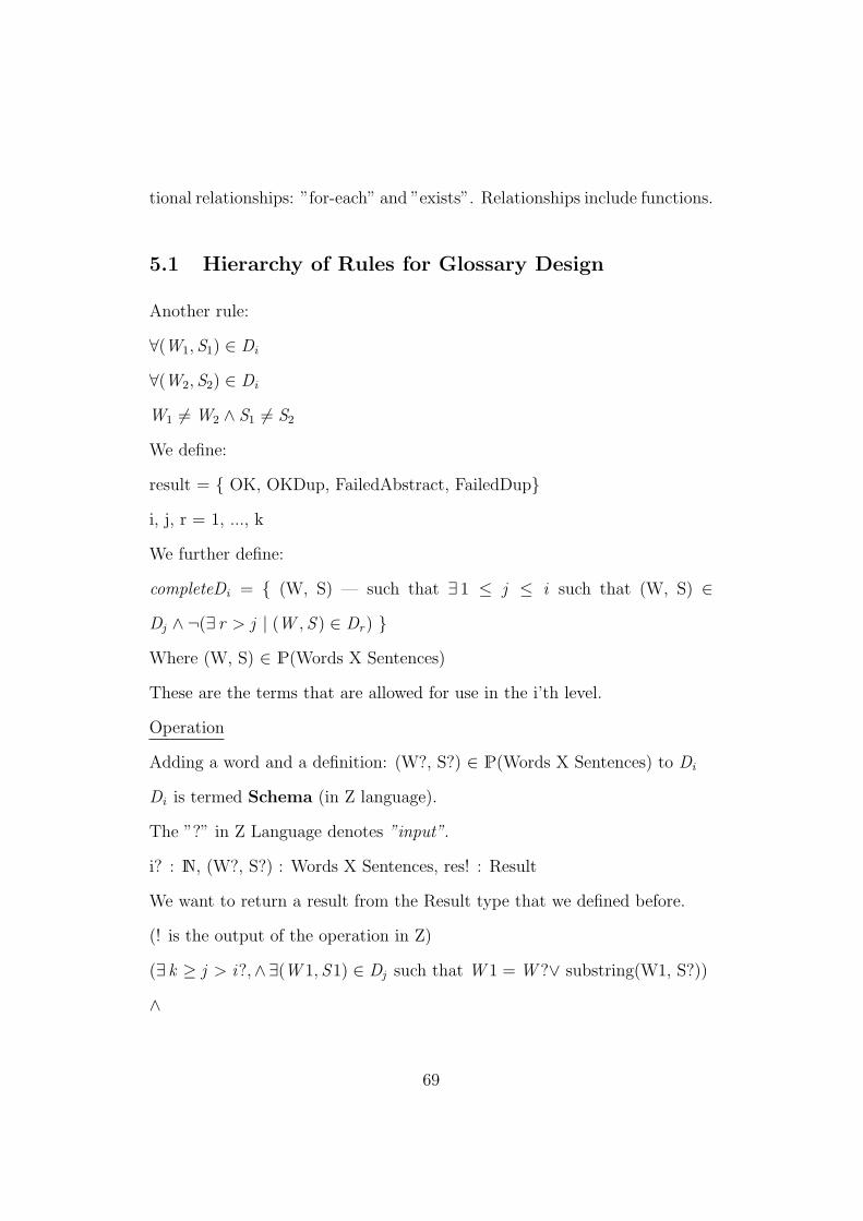
tional relationships: ”for-each” and ”exists”. Relationships include functions.
5.1 Hierarchy of Rules for Glossary Design
Another rule:
∀(W1, S1) ∈ Di
∀(W2, S2) ∈ Di
W1 6= W2 ∧ S1 6= S2
We define:
result = { OK, OKDup, FailedAbstract, FailedDup}
i, j, r = 1, ..., k
We further define:
completeDi = { (W, S) — such that ∃ 1 ≤ j ≤ i such that (W, S) ∈
Dj ∧ ¬(∃ r > j | (W , S ) ∈ Dr) }
Where (W, S) ∈ P(Words X Sentences)
These are the terms that are allowed for use in the i’th level.
Operation
Adding a word and a definition: (W?, S?) ∈ P(Words X Sentences) to Di
Di is termed Schema (in Z language).
The ”?” in Z Language denotes ”input”.
i? : N, (W?, S?) : Words X Sentences, res! : Result
We want to return a result from the Result type that we defined before.
(! is the output of the operation in Z)
(∃ k ≥ j > i?,∧∃(W 1, S1) ∈ Dj such that W 1 = W ?∨ substring(W1, S?))
∧
69

which means that the result is:
res! = FailedAbstract
Y
(∃(W 1, S1) ∈ Di such that W 1 = W ?)
∧
res! = FailedDup
Y
(∃ 1 =< j =< i(W 1, S1) ∈ Dj and W 1 = W ?)
∧
D′
i - the situation of the dictionary after the operation
D′
i = Di ∪ {(W ?, S?)}
res! = OKDup
OKDup = we can define again a term that we defined in a previous level
Y
D′
i = Di ∪ {(W ?, S?)}
∧
res! = OK
Next, we prove by induction on the operation that if we start with the dic-
tionary Di = ∅ (the atom) and define the operation as the schema, then we
can use the inductive set proof method to prove that all resulting dictionaries
preserve the same rules. Intuitively, this is clear, since our only operation
adds—without breaking the rule.
Hierarchical Glossaries Example, Continued
We denote the hierarchy of dictionaries as D1, D2, ... Dk . Each Dictionary
Di is of type P(Words X Sentences) where 1 ≤ i ≤ k. In words, each dictio-
70

nary is a set of pairs of words (dictionary terms) and sentences (the term’s
meaning). Another way of saying it is that Di : P(Words X Sentences). X
”:” Y denotes that X is ”of type” Y3.
Let’s see how it works:
A sample of a set in Di (a semantic example):
{(cat, ”an animal which I have at home”), (dog, ”an animal that I don’t have
at home”), (snake, ”an animal I found yesterday in my yard”)}
Another example: {(”abc”, ”e”), (”abc”, ”abc”), (”abc”, ”d”)} is a dictio-
nary since the syntax is legal (even though the semantics might not make
much sense).
Another example: {(” abc”, ” abc def ”), (”abc”, ”d”)} is not a dictionary
since the first term includes a space, which is illegal in the syntax we defined.
5.2 Introducing the Z Specification Language
The Z language includes:
• First order logic (propositional calculus and ordinal calculus): ∧, ∨,
→, ¬
• Relations and functions: ∀, ∃
• Each set has to be of a type; we do not allow all the possible sets. For
instance, we do not want to have sets of the type: {Tomato, Volvo,
Roof} since they are members of different types.
The type is a tool that enables testing the consistency of the definition of a
specification.
3which is also saying that X is a member of Y
71

∀ i : N, 1 ≤ i, ∧ i ≤ k, ∀ (W, S) ∈ Di , W 6= S
This means that the term and definition will be different.
The error in the definition is that we cannot compare things of different
types: W 6= S, Words and Sentences are not of the same type. So—an open
question—how do we overcome this obstacle? It’s not easy! It requires more
knowledge of the Z language.
This definition is actually an ”invariant”; that is, it is true throughout the
whole lifecycle of the system.
∀ i : N, 1 ≤ i, ∧ i ≤ k, ∀ (W1, S1) ∈ Di , ∀ (W2, S2) ∈ Di , W1 = W2 → S1
= S2
This means that each term has only a single definition.
That is, for every two pairs of words and sentences in the dictionary, if the
word is the same word, the definition has to be the same too. This is also an
invariant.
∀ w : Words, ∀ s : Sentences
substring : Words X Sentences → {T, F}
substring(W, S) = T ⇔ ∃ i ∈ N, ∀ j such that #W+i > j ≥ i, W(j - i) =
S(j)
substring is a function from pairs of words and sentences to a set of True,
False.
What is a function? A function associates each value from the source (in our
case, Words X Sentences) with a single member in the target (True or False).
#W is the length of the string W.
Example
Prove that ’ab’ is a substring of ’drabf’.
72

#’drabf’ = 5
We take i to be 2. j is the values from i = 2, and to the length of ’ab’ #’ab’
= 2, 2+2=4; thus j is the values from 2 to 4.
Future Enhancements
In the next lecture (see section 6) we will attempt to define operations such
as addition and removal. For that, we need to better improve the definition
of our world and notations.
Our world consists of a series of documents. Each document is specified with
a specific dictionary:
D1 ↔ SP1 (Specification)
D2 ↔ SP2 (Specification)
D3 ↔ SP3 (Specification)
and so on...
Now, we’d like to define a new document, SP5, with a dictionary D5. The
question is, what terms am I allowed to use and not allowed to use in SP5?
We decide that we are not allowed to use any terms defined after 5, and we
are allowed to use the latest added definition of any term defined before 5.
We define CD1, CD2, ... CDk : P(Words X Sentences) where each CDi (cur-
rent dictionary) is the words allowed for use in the specification SPi .
∀ i, 1 ≤ i ≤ k, (w, s) ∈ CDi , max(w) ≤ i
This means that (w, s)—a word and its definition—is in the current dictio-
nary, if the maximum appearance of the term is before i, where max(w) is
the maximum place in which w appears.
max : Words → N
max(w) = i ⇔
73

(∃ s ∈ Sentences ∧ j ≤ i, (w, s) ∈ Dj ) ∧ (¬ ∃ s ∈ Sentences ∧ j > i, (w, s)
∈ Dj )
5.3 Hierarchical Dictionaries Example, Continued
We define the term ”thread”. In D1 we define ”thread” as a string. In D4
we define ”thread” as a light computer process. In any specification using
dictionaries greater than or equal to level 4, ”thread” means the ”light com-
puter process” definition.
CDi—where i = 1, 2, ..., k—is the set of words that you can use at level i.
Note that to reach a specific definition, we can use examples, drawings, and
diagrams, and write ”in words” the definition before we write it formally.
Let’s try and define CDi formally. CDi is a set of Words and their Definition.
The use of the set usually indicates the use of P. Words and their definitions
are indicated by Words X Sentences.
So CDi is of type: P(Words X Sentences), which means a set of pairs, and
each pair is an instance of Words and a defining instance of Sentences.
Example
CDi = {(”thread”, ”light weight computer process”), (”CSP”, ”Constraint
Satisfaction Problem”)}
We defined that at each level we’d like to use only terms that appeared before
the level (and not just after the level), and in that case, we’d like to use the
most up-to-date relevant definition.
(w, s) ∈ CDi ⇔ ∃ j ≤ i, (w, s) ∈ Dj . In words, this means that a pair of
word and sentence, is legal in dictionary of level i CDi if and only if there
74

exists a j, smaller or equal to i, where the pair of word and sentence is in the
dictionary of level j.
Next, we would like to add the definition of using the latest, most currently
available version: (w, s) ∈ CDi ⇔ j ≤ i, (w, s) ∈ Dj ∧ ∀ l, k : N, (l ≤ i) ∧
(k ≤ i) ∧ l < k ∧ (w, s1) ∈ Dl ∧ (w, s2) ∈ Dk → (w, s1) 6∈ CDi
In words, if k and l are dictionaries before i, and l is before k, and (w, s1) is
in dictionary l, and (w, s2) is in dictionary k, then (w, s1) can’t be in the list
of allowed words in level i.
Note, the Z specification language is a declarative and not operative lan-
guage, so we define formal definitions without defining how we can opera-
tively reach it.
Example
We would like to reach a simpler definition, possibly using the ”max” func-
tion.
5.4 Defining Adding a Word and its Definition to a
Dictionary
We formally define the addition of a term and its definition to a dictionary
Di . In the Z specification language, we use ”?” to denote input. We would
like to add (w?, s?) : Words X Sentences to dictionary Di . We define an
output, or result, which is the updated dictionary (a side-effect change), and
a response, which is the result of the operation. We mark the resultant
output using ”!”.
We begin with defining when we would like to allow the addition of a pair
75

(w?, s?) to dictionary Di .
1. If (w?, s1) is already in Dictionary Di , what do we want to do? We
would like to tell the user that we are overriding the definition (adding
the new definition to replace the old one). In the case S1 is different
than s?, so we mark the response okDup.
2. Same as in #1 but for the case that s1 = s?, we mark the response as
okCompleteDup.
We gradually define the Result set with all the possible responses. Result =
okDup | okCompleteDup.
We gradually define the operation formally, defining a schema in Z as follows:
i? : N, 1 ≤ i? ≤ k ,
(w?, s?) : WordsXSentences ,res ! ∈ Result
∃ s1 ∈ Sentences ,(w?, s1) ∈ Di ⇒D ′
i = (Di ∪ {(w?, s?)})\{(w?, s1)}∧s1 6= s? ⇒ res ! = okDup∧s1 = s? ⇒ res ! = okCompleteDup
Above the line, we define the input and output. Below the line, we define
the different cases.
The first case says that if a sentence for the word we would like to add already
exists in the dictionary, the dictionary after the operation is the dictionary
with the new sentence, and we remove the previous definition.
Exercise
Prove using induction that each word that appears in dictionary Di appears
76

only once.
Hint: The atoms ∅ = D1 = D2 = ... = Dk , and the operations P add a word
and a sentence (w?, s?) to dictionary Di .
5.5 Dictionary Example
Assume we have dictionaries D1, D2, ..., Dk as before, and the term byte only
appears in level D6, but in D2 ”byte” is used in the definition of term w. Is
this acceptable? Do we want to allow defining terms using disallowed terms?
We would like to prevent the option of adding a defining sentence for a term
that uses terms that are disallowed in the dictionary level to which the term
is to be added.
We add another case (denoted by ∨) to our previous definition: ∃ w1 : Words,
substring(w1, s?) ∧ w1 6∈ CDi ⇒ res! = Fail
which means a word w1 exists, in the defining sentence s? which we would
like to add to dictionary Di , but w1 is disallowed in CDi , so the operation
should fail. In the case of a failed result, we do not change the dictionary.
We update the Result set to be:
Result = okDup | okCompleteDup | Fail
5.6 Referred Sets
When defining a formal specification, to which sets are we allowed\not al-
lowed to refer?
We will use induction for defining the sets we are allowed to use, with oper-
ations Cartesian Product and Power Set. We define these as the basic types.
77
We define the Atoms: [A1], [A2], ... , [Ak ]
For instance, [Result] = [ okDup | okCompleteDup | Fail]
and we define the operations: P and X.
Therefore, we conclude that P(A2 X A3) is also a type.
Note that all the sets to which we are allowed to refer must be subsets of
allowed types.
Exercise
Assuming the atoms: [{1, 2, 3}], [{4, 5}] Are the following allowed types or
not?
1. {3, 4} is disallowed since we can’t reach this set from activating Power
Set or Cartesian Product on the atoms. We can’t refer to this set, since
it is not a subset of any existing type.
2. { {3}, {4} } is not a type because we won’t reach this set from the
basic types (atoms) and the operations. If it is a set we are allowed to
refer to, we need to show a derivation order of operations that results
in a set containing this set. We can’t do that without an additional
parenthesis: { ({3}, {4}) }.
3. {1, 2} is not a type, but we are allowed to refer to it since it is a subset
of a type.
5.7 Z Specification Language Basic Signs
We started talking about some of the basic signs of the Z specification lan-
guage. Z is a very rich language, with many additional signs. The use of
78

many signs has not been proven to improve readability or quality.
We discussed the restrictions of the Z language that cause us to be more spe-
cific, and find problems in the specification and software. We use Z to define
what a software program is supposed to do (and not how). We discussed the
use of ”types”.
Why aren’t requirements a part of software development? Because require-
ments aren’t just for software development. Defining functions is also needed
in other domains.
The Z specification language includes first order logics, group theory, and
types.
First order logics includes, for instance, ∨, ∧, ¬, →, ∀, ∃, signs for functions
and relations, functions (f, g), relationships (R, S, T), and so on.
Group theory includes ∈, ⊆, ∪, ∩, P, X (Cartesian Product), and so on.
The term ”Types” includes only the certain types that we are allowed to
refer to (all the members need to be of the same ”type”).
Our purpose in this lecture for each specification is to define the types to
which we are allowed to refer.
We define the types we are allowed to refer to using induction. Types are
defined as the groups that we are allowed to refer to in each specification.
We are allowed to refer to any group that is a type or that is a subset of a
type.
Note: The requirement makes a distinction on the operations that you can
perform. For instance, if you take a ∪ on two groups that you are allowed
to discuss, you are not necessarily allowed to refer to the union of the two
groups.
79

To define all the types we are allowed to refer to for a specific specification,
we use an inductive set.
We use a set of ”basic types” that we are allowed to refer to—even though
we cannot define them—as the atoms of the inductive set. We mark them
as [A1], [A2], ..., [Ak ]. In each system, there will be basic types.
Exercise
What are the basic types in the definition of the glossaries?
Union (∪) between types cannot be used to define a new type. So we redefine
the union operation:
A ∪ B = { x | x ∈ A ∨ x ∈ B } ⇔ ∃ R ∈ I(A, P), A ⊆ R ∧ ∃ S ∈ I(A, P),
B ⊆ S ∧ R = S
That is, A and B are subsets of the same type.
Next, we define a relation:
R is a relation if R ∈ P(A X B), where A and B are types. In other words,
R is a relation if it is a set of couples: a from A, and b from B, and A and
B are types.
Example
Our basic types are [C = {a, b, c}], [D = {0, 1}].
C X D = {(a, 0), (a, 1), (b, 0), (b, 1), (c, 0), (c, 1)} is a type.
The following is a relation: {((a, 0), 0), ((a, 0), 1)} because it is a set which
is a member of ((C X D) X D).
Function is a specific example of the relation f: P(A X B) where f is a relation
and for each member of the source (A) there is a single member in (B), which
means there is a single couple in f.
80

6 Lecture - Formal Specification Languages
Lecture Outline
• Rules for Design of Glossaries Hierarchy, continued
• Sets
• Type
• Cartesian Product Sets
• Functions
• Bijective Function
• Equivalence Classes
• Fixed Point Theorem
In the previous lecture we discussed specifications as definitions of what a
system is supposed to do. We use mathematical logic and set theory.
We ended the lecture with a sample specification and found that it was in-
correct (to be revisited in a later lecture).
In this lecture, our aim is to define the formal language used for specifications.
While defining, we try to provide examples of snippets of specifications.
Our discussion is limited to sets whose members are only of the same type.
For example: { Subaru, USA } is not a set we refer to, as Subaru is a type
of car and USA is a country, so they are not of the same type.
We present, in parallel, the formal language syntax and its associated inter-
pretation (semantics).
81

6.1 Formal Specification Language - Definition
Syntax
Our purpose is to define the sets that we are allowed to refer to. We define
the following symbols by induction:
1. Assuming k symbols: [A1], ..., [Ak ].
2. If Y and Z are allowed symbols, then Y X Z and P(Y) are also allowed
symbols.
3. We define I(A, P) as the set of all possible allowed symbols.
The intended meaning of these symbols is the possible set types.
Interpretation
To create a specification, we map [A1], ..., [Ak ] to k sets A1, ..., Ak , and define
the inductive set I(A, P) as the set of possible types where X is interpreted
as the Cartesian Product operation and P as the Power Set operation.
Example
A1 = {Subaru, Volvo, Fiat}
A2 = {Slow, Fast, Medium}
A1 X A2 = {(Subaru, Fast), (Subaru, Slow), (Subaru Medium), ..., (Fiat,
Medium)}
P(A1 X A2) = {∅, {(Subaru, Fast), (Fiat, Fast)}... }
| A1 X A2 | = 9
| P(A1 X A2) | = 29
Members of P(A1) X P(A2) are pairs of subsets of A1 and subsets of A2.
A sample member: ({Subaru, Volvo}, {Fast, Slow}) ∈ P(A1) X P(A2).
82

We limit our discussion to (the specification can only refer to) subsets of sets
that are types, or members of sets that are types.
Syntax
• ∈ Interpreted as a member of
• ¬, ∧, ∨, → Interpreted as in propositional logic
• ⊆ Intended interpretation is subset
F ⊆ G ⇔ (x ∈ F ⇒ x ∈ G) ∧ ∃ H ∈ I(A, P) : G ∈ H
The intended meaning is that F is a subset of G if and only if for every x
which is a member of F, x is also a member of G. In ”regular” set theory, this
definition is sufficient. In our scope we add to this definition an additional
requirement that G be a member of some set H ∈ I(A, P). H must be a type
we are allowed to refer to.
Semantics
Same A1 and A2 as before.
Now we check if one set is a subset of the other:
Is the following true?
{Subaru, Fast} ⊆ {Subaru, Volvo, Fast}
No! Why? Because the members of the set do not belong to a single type.
In ”regular” set theory, this would have been True, since x ∈ A ⇒ x ∈ B,
but in our language, this is not True since both sets do not belong to any
single type.
{Subaru, Volvo, Fast} 6∈ I(A, P)
Claim
83

Any member of I(A, P) that is not A1 or A2 has a size of at least three
members. Note that each member of I(A, P) is a set.
Proof by induction
For the Atoms, the statement is true. Assuming Y and Z are members of
I(A, P) and | Y | > 3 and | Z | > 3, then | P(Y) | > | Y | > 3, | P(Z) | > |
Z | > 3, | Y X Z | > | Y | > 3.
What is missing in the definition?
Example of building I(A, P) on different sets:
A1 = {a, b}
A2 = {c, d}
P(A1) = {∅, {a}, {b}, {a, b}}
P(A2) = {∅, {c}, {d}, {c, d}}
A1 X A2 = {(a, c), (a, d), (b, c), (b, d)} A1 X P(A1) = {(a, ∅), (a, {a}), (a,
{b}), (a, {a, b}), (b, ∅), (b, {a}), (b, {b}), (b, {a, b})}
P(P(A2)) = {∅, {∅}, {{c}}, {{d}}, {{c, d}}, {∅, {c}}, ...}
We continue with the syntax. We defined a member, types, basic operations,
and so on. What’s next? Let’s define equality:
A = B ⇔ A ⊆ B ∧ B ⊆ A ∧ [ ∃ C : I(A, P), (B ∈ C) ∧ (A ∈ C)]
∃ C : we will need to denote of which type is C.
Whenever we refer to ∃ x and ∀ x, we need to define the set over which x is
known as a valid set.
∀ x ∈ A and ∃ x ∈ A are valid ⇔ A ⊆ C
We add the definition of a relation, R:
R is defined as R ⊆ Y X Z where Y and Z are types.
In other words, R is a set of pairs.
84
Summary
So far, in our syntax, we allow the use of:
• Sets: [A1], ..., [Ak ]
• I(A, P) - types
• ∈
• ⊆
• =
• ∃
• ∀
• R - relation
Relative definition
[A1], ..., [Ak ]
I(A, P) - types
And for
∈
⊆
=
∃
∀
R - relation
We add the restriction of types.
85

6.2 Ruling Function from the Talmud Revisited
The ruling function from the Talmud is described in section 1.4.
We continue the definition with a justification for referring to the types:
P ⊆ (A X A) X Payment
Payment ∈ P((A X A) X Payment)
So our discussion about this relation is valid. If, for instance, we define a
function f from A X A to Outcomes:
f : A X A → Outcomes
f = {((don’t know, don’t know), 0), ((don’t know, A), 500), ... , ((B, B),
1000)}
Let’s verify if f is a type.
[Outcomes = {0, 500, 1000}] and is a type, since it is a basic type.
We had [Costs = {500, 1500, 2000}], which we do not use, so we can remove
it. On the other hand, Costs describes the cost of the bulls, so we might need
it later.
We notice that Costs ∩ Outcomes 6= ∅, which isn’t ”elegant” since it is rare
for intersections between basic types to be not empty.
We can solve this, for instance, by referring to [N] as the basic type of the
natural numbers, which makes Outcomes and Costs subsets of N, so we are
allowed to discuss Outcomes and Costs:
Outcomes ⊆ N, Costs ⊆ N.
If we decide that Outcomes is a basic type, what is the type of function f?
Since f ⊆ (A X A) X Outcomes
f is of type
86

f : P((A X A) X Outcomes)
Since A and Outcomes are basic types, and we are allowed to use the Carte-
sian Product and Power Set operations, (A X A) is a type, (A X A) X
Outcomes is a type, and P((A X A) X Outcomes) is a type.
We use the fact that if C ∈ D and D is a type, then C : D.
In other words, if C ⊆ E ⇒ C ∈ P(E).
If we decide that Outcomes is not a basic type, and we use N as a basic type:
f : P((A X A) X N)
Exercise
What is the type of function f if we were to define both Costs and Outcomes
as basic types?
We leave this as an exercise for the reader.
Summary
• Set Theory
• Logics with quantifiers
• Logics with Types, defining a language that helps define what software
is supposed to do
• Example from the Talmud (with Bulls), modeled using a function
87
7 Lecture - Communication Group Example
We want to model which computers / end-points are in touch with which
others, and can transfer data. We term the example: ”Group Communica-
tion”.
We aim to define a group of computers that all share the same set of mes-
sages, although each computer can be either in an up or down state, and the
communication between them can fail.
Potentially, because we do not restrict the network, each computer can com-
municate with all other computers.
We begin by describing the state of each computer. We term the computers
Nodes. Each Node can be in one of two states: {up, down}.
A node in the down state cannot communicate with other nodes, and other
nodes cannot communicate with that node. A node in the up state can po-
tentially communicate with other nodes that are up.
We define the Nodes as a basic type: [Nodes]. We start with two groups:
[Nodes], [States = {up, down}]. The symbol ”[]” marks Basic Types.
We allow referring to the basic types and the inductive set induced by the
basic types and the operations: Cartesian Product, marked by X, and Power
Set, marked by P.
We define [Nodes] as the set of computers in the network. We define [States]
as an attribute state of the computer: up, i.e., which is up and running; or
down, i.e., not running.
The purpose of the formal definition is to define a situation where only ma-
chines that are up can be connected in a Communication Group, and ma-
88

chines that are down cannot be in the Communication Group (which also
makes sense intuitively).
We aim to model changes in states in the Communication Group (machines
changing status from up to down, and vice versa).
We mark the [Nodes] basic type as N, and the [States] basic type as S.
The next thing we need is a name for the computers. We agree that there is
a unique number indicating each computer. So, we use the N basic type to
indicate the nodes: [Nodes : N].
We reduce the number of Nodes to a finite number of nodes, so Nodes ⊆ N
⇒ Nodes ∈ P(N). P(N) is a type because N is a basic type, and so N is a
type and therefore P(N) is a type.
We claim that: f : Nodes → States. What does this mean? f is the function
that maps a state to each node. f ⊆ Nodes X States, States is a type, Nodes
⊆ N and N is a type. A general function f: A → B is a ⊆ A X B.
Therefore, f ∈ P(N X States), and P(N X States) is a type.
Next, we define Connected as a set of all the computers (Nodes) connected
to one another.
Connected : P((NXS )X (NXS ))
∀(n1, s1), (n2, s2) : NXS((n1, s1), (n2, s2)) ∈ Connected →s1 = s2 = up
Example
{((1, up), (4, up)), ((4, up), (3, down))} is not Connected because node 3
is down.
89

Next, we define a function from Nodes to their States:
state : Nodes → States.
In this case the function is a complete function because for each member n of
the source (Nodes in our case) there is a single value in the target (States),
which is state(n).
state : P(NodesXStates)
(∀ n ∈ Nodes ,∃ s ∈ States(n, s) ∈ state)∧(∀ n : N ,∀ s1 : S ,∀ s2 : S ,
(n, s1) ∈ state ∧ (n, s2) ∈ state → s1 = s2)
To verify that state, which is of type P(Nodes X States), is something to
which we can refer, we need to verify that P(Nodes X States) is a type.
[Nodes] is a basic type and therefore a type. [States] is also a basic type and
therefore a type. Nodes X States is also a type since the Cartesian Product is
an allowed operation between types. P(Nodes X States) is also a type since
the Power Set is an allowed operation on types.
We define Connected as a requirement that is an invariant.
We attempt to define the operations in the system, starting with the ”easier”
action. But first we need to define the initial state of the system.
In the initial state, we would like the invariant to be correct and to define
the state of each node.
For instance, if the Connected set is empty (∅), it preserves the invariant.
Another option is that all the states of the nodes are up (no matter what
that set Connected contains).
90

Initial State
Next, we aim to define the Initial State:
state : N → S
connected = ∅∧∀(n, s) ∈ state, s = down
This schema means that the initial state is that all computers (nodes) are
down.
We next aim to model the operations and changes that can occur in the
system, and we start with a fail.
Fail((n1, s1), (n2, s2))? : P((NXS )X (NXS ))
((n1, s1), (n2, s2)) ∈ connected∧connected ′ = connected − {((n1, s1), (n2, s2))}
Example
We assume the set Connected is {((1, up), (2, up))}.
Our input is: ((1, up), (2, up)).
The predicate calculation is ((1, up), (2, up)) ∈ connected is true and
Connected’ = Connected - {((1, up), (2, up))} = {((1, up), (2, up))} - {((1,
up), (2, up))} = ∅.
If the input was illegal; for example, our input is: ((1, up), (2, down)), then
(((1, up), (2, down)) ∈ Connected) is false, and therefore Connected’ remains
unchanged
91

Fail Noden? ∈ Nodes
State(n?) = up∧State ′(n?) = down∧∀ n∼ ∈ Nodes , s∼ ∈ States ,((n?, s), (n∼, s∼)) ∈ Connected →Connected ′ = Connected − {((n?, s), (n∼, s∼))}∧((n∼, s∼), (n?, s)) ∈ Connected →Connected ′ = Connected − {((n∼, s∼), (n?, s))}
Note: To activate the operations: ∪ and ∩ on sets, both arguments (sets)
need to be of the same type and therefore when we write Connected’ =
Connected - something, that something has to be a set.
Example
State = {(1, up), (2, up), (3, down), (4, up)}
Connected = {((4, up), (1, up)), ((1, up), (2, up))}
We activate Fail Node on node n? = 1:
(State(n?) = State(1) = up) = True
State’ = {(1, down), (2, up), (3, down), (4, up)}
Connected’ = Connected - {((4, up), (1, up))} - {((1, up), (2, up))} = ∅
We use sets A and B to help us with the operation
A = {((n?, s), (n∼, s∼)) : P((N X S) X (N X S)) | ((n?, s), (n∼, s∼)) ∈
Connected } ∧
B = {((n∼, s∼), (n?, s)) : P((N X S) X (N X S)) | ((n∼, s∼), (n?, s)) ∈
Connected } ∧
Connected’ = Connected - (A ∪ B)
92

Node Backn? : Nodes
State ′(n?) = up
Connection Back((n, s), (n∼, s∼))? : P((NXS )X (NXS ))
State(n) = up∧s = up∧State(n∼) = up∧s∼ = up∧Connected ′ = Connected ∪ {((n, s), (n∼, s∼))}
or, in a simpler yet equivalent way:
Connection Backn : Nodes , n∼ : Nodes
State(n) = up∧State(n∼) = up∧Connected ′ = Connected ∪ {((n, up), (n∼, up))}
93

8 Lecture - Communication Group Example,
Continued
In this lecture we continue with the Communication Group example.
The modeling process we are discussing, as a whole, is part of the larger
review process, which is a process intended to find problems and issues of
concern.
We use the methods to find problems:
1. Exact writing
2. Simulation according to an example
3. Writing proof
Bugs are much more costly when found in the customers’ sites, as opposed
to finding them during the design phase.
So why don’t organizations spend more time on finding design problems?
Nearly 80% of projects fail. So why aren’t these design methods implemented
to find problems? The answer is that people don’t know how to perform them
or use them effectively.
Usually, a simple model is only generated the third time a model is written.
One of the best practices in software development is to rewrite your code;
i.e., throw away the original and write it again from scratch.
Communication Group Example, Continued
We start with two groups (basic types): [Nodes], [States = {up, down}].
In our world we are allowed to refer to basic types and recursive activations
94

of the operations; the Power Set and Cartesian Product. We can mark them
like this: I(([Nodes], [States]), (X, P))
nodeState : P(NodesXStates)
nodeState : Nodes → States
The → indicates that this is a function; that is, nodeState is a function (in
this case, a full function).
Connection : P(nodeState)
x ∈ Connection ⇔| x |= 2
The idea is to look at the arcs, which are connections between nodes of size
two.
For example, Connection = {{(A, up), (B, up)}, {(A, up), (E, up)}, {(B,
up), (E, up)}}.
Node Downn? : Nodes
nodeState ′(n?) = down∧Connection ′ = Connection\{{(n1, s1), (n2, s2)} ∈ Connection| n1 = n?}
Node Upn? : Nodes
nodeState ′(n?) = up
95

Add Connection(n1, s1)?, (n2, s2)? : (NodesXStates)
s1 = s2 = up∧Connection ′ = Connection ∪ {{(n1, s1), (n2, s2)}}
Remove Connection{(n1, s1), (n2, s2)}? : Connection
Connection ′ = Connection − {{(n1, s1), (n2, s2)}}
Example
We focus on the consistency of the group, which ensures that the model is
correct. There are other possible focus areas that we do not deal with.
Our purpose is to characterize a set of nodes that are possibly communicat-
ing with one another. Each node can either be in a state of up or down. It
is not possible for two nodes that are not both up to be connected.
We define an initial state in which all the nodes are ”down” and the Com-
munication Group is empty (there is no communication between any of the
pairs).
Nodes can change state to up or down, and communication couples can be
added or removed. There are options to add/remove nodes.
We began with the definition of two basic types: [Nodes] and [States = {Up,
Down}].
nodeState is a relation (a function) from Nodes to States.
f : Nodes → States
f : P(Nodes X States)
96

Next, we check the type of the Communication Group (Connection) set to
verify it is a type we can refer to.
Reminder: Connection is a set of subsets of Nodes where the size of each
subset is 2. We denote this in formal writing as:
Connection : PP(Nodes) | x ∈ Connection ⇒ | x | = 2
This definition and specification differs from our previous definition of the
Connection set in that in this definition the connection between two nodes
is not directed.
Note: There is a hidden decision taken here, not specifically stated in the re-
quirements. At this phase of the software development process, it is ”cheap”
to change the design between a Connection set which is directed, and one
which is not. Changes performed during the design phase are cheap, because
they are performed before a few hundred lines of code are written.
We adjust our invariant for the indirected connection between nodes, or in
formal writing:
({n1, n2} = x ∈ Connection ⇒ (f(n1) = Up ∧ f(n2) = Up))
Another way to write the invariant, is that for any node that is down, the
node cannot be in the Communication Group.
We continue by writing the operations explicitly in formal writing, and start
with the Node Up operation:
Node Upn? : Nodes
f ′(n?) = Up
97

Node Down is more complicated, since it also needs to check in which con-
nections the node participates, and disconnect those connections. If we don’t
disconnect those connections - the invariant will be broken.
Node Downn? : Nodes
f ′(n?) = Down∧Connection ′ = Connection−{x = {n1, n2} ∈ Connection| n1 = n? ∨ n2 = n?}
The way to come up with the correct formal writing of the operations typ-
ically involves a roundabout process in which the requirements are defined
in words and then translated to formal writing of the specification. In doing
so, we find that there are missing details in the requirements. We correct
the requirements, refine the formal specification, and so on in a roundabout
process.
The Connection Up and Connection Down operations in formal writing are:
Connection Up{n1, n2}? ∈ P(Nodes)
f (n1) = Up∧f (n2) = Up∧Connection ′ = Connection ∪ {n1, n2}
Connection Down{n1, n2}? ∈ P(Nodes)
Connection ′ = Connection \ {n1, n2}
98

Communication Group : P(Nodes)
∀ n1, n2 : Nodes(n1, n2) ∈ Connection
Reminder: The Communication Group is the set of nodes such that each
node is connected with any other node in the set.
We add an initial state for the Communication Group to be the empty set
∅.
Question
Do the operations Node Up and Node Down change the Communication
Group?
Answer
In the current definition, there can be many Communication Groups, since
we did not define it as the maximal group.
Therefore, we would like to add to the definition that the Communication
Group must be the maximal group.
To make the Communication Group a single group, it will need to be a set
containing the previous definitions, that is, a set of subsets in which each
node is connected.
But, in this case, the definition becomes too complicated, and is out of the
scope of this lecture.
To summarize what we have so far:
We defined the operations: Node Up, Node Down, Connection Up and Connection Down,
an invariant and an initial state.
Claim
99
Prove that the invariant is preserved in any state of the system.
Proof
We prove using induction.
We begin with the initial state. For the atoms, we need to show that ∀ n :
Nodes, f(n) = Down.
Since Connection = ∅, it is preserved by the empty set of couples that for
every couple in Connection {n1, n2} ∈ Connection, n1 and n2 are both in the
Up state, because there are no couples.
Next, we assume that the invariant is true; that is:
∀ {n1, n2} ∈ Connection, f(n1) = Up ∧ f(n2) = Up.
In the inductive step, we activate the different operations and show that the
invariant is still preserved. We iterate through the operations, beginning
with the Node Up operation:
There are two options:
• If, before the operation, f(n?) = Down, then according to the inductive
assumption, n? was not in Connection. Therefore, after the operation,
the invariant is still preserved.
• If, before the operation f(n?) = Up, then according to the inductive
assumption, n? might or might not have been in Connection. In this
case, n? stays Up, so we did not change Connection.
To avoid needing to check two options in the proof, we could add a test to the
Node Up operation that checks the state of the node before the operation.
100

Corrected Node Upn? : Nodes
iff (n?) = Down → f ′(n?) = Up
Next, let’s prove for the Node Down operation. Again, there are two options:
• If, before the operation, f(n?) = Up, then in the Connection Group
before the operation, Connection = { {n1, n2} : P(Nodes) | (n1 6= n?
∧ n2 6= n?) ∧ {n1, n2} ∈ Connection} ∪ { {n1, n2} : P(Nodes) | (n1
= n? ∨ n2 = n?) ∧ {n1, n2} ∈ Connection}. In words, we separate
the Connection set into the pairs in which n? participates and those in
which n? does not participate.
• If, before the operation, f(n?) = Down, then according to the inductive
assumption, n? wasn’t in the Connection group.
We leave the reader to similarly iterate through the other operations to com-
plete the proof.
101

9 Lecture - Communication Group Example,
Continued
Revisiting the Communication Group example, we find a different—more
effective—interpretation and specification. We begin with the initial state
definition:
Initial State
∀ n : NodesnodeState ′(n) = Down∧Connection ′ = ∅
Next, we formally describe the operations:
Connection Upn1?, n2? : Nodes
nodeState(n1?) = Up∧nodeState(n2?) = Up∧Connection ′ = Connection ∪ {n1?, n2?}
The basic types we use are [Nodes] and [States = {Up, Down}]. We addi-
tionally define the function: nodeState of type Nodes → States. We define
the Connection set using the following schema:
Connection : PP(Nodes)
x ∈ Connection ⇔| x |= 2
The invariant can then be written as this:
102

Invariant
x = {n1, n2} ∈ Connection ⇐(nodeState(n1) = Up ∧ nodeState(n2) = Up)
We continue with the revised operations:
Node Downn? : Nodes
nodeState ′(n?) = Down∧Connection ′ = Connection−{x ∈ Connection | n? ∈ x}
Node Upn? : Nodes
nodeState ′(n?) = Up
Connection Downx? : Connection
Connection ′ = Connection − x
Let’s review the process; we started with a model. We then noticed that
the model describes a directed graph. That is, the connections between the
nodes in the Communication Group were directed, so we decided to recreate
the model from scratch as an indirected graph.
We then discovered the model can be written in a simpler manner if we don’t
write the state for each node in the graph, but rather only use the nodeState
function on the nodes. This is a classic process of making things simpler by
103

iterations of specifications.
Simpler models preserve that they make are easier to find problems in, and
are easier to use to find problems in the system requirements.
This is a third iteration of the model, and we use it in this lecture to analyze
if it is correct. There is an interesting trade-off that says that as long as you
can continue claiming on the system then the system can be simpler, and
still hold true.
Claim
Our invariant claim is that for each member in Connection, both nodes have
a node state that is Up.
Proof
To prove the claim we need to start from the initial state where there are no
connections and all nodes are down and apply the operations in any order,
showing that the invariant is preserved. In the proof we use the inductive
set induced from the initial state and the defined operations. For the initial
state, the invariant is true according to the definition of the empty set, as
in the empty set there are no connections. In the inductive step, we assume
the invariant is true for any member of the inductive set, and need to prove
that the invariant is still preserved after activating any of the operations on
the members of the inductive set.
Any operation that is not invoked does not change the Connection set, and
therefore the invariant is preserved.
We iterate through the operations. For operation Node Up, the input is n?.
There are two options:
1. n? is not a member of x, where x ∈ Connection and Node Up does not
104

add any new members to Connection, so n? is not a member of any
pair in Connection after activating the operation.
2. n? is a member of x, where x ∈ Connection. According to the in-
ductive assumption, nodeState(n?) = Up, and the Connection is left
unchanged. According to the inductive assumption, the Connection set
preserves the invariant.
For operation Connection Down, there are again two options:
1. {n1?, n2?} is a member of Connection.
According to the inductive assumption, the invariant claim is valid for
the Connection set, and so it is also valid for the set after removing the
pair: Connection’ = Connection - {n1?, n2?}.
2. {n1?, n2?} is not a member of the Connection set, and so Connection
is unchanged. According to the inductive assumption, Connection pre-
served the invariant before the operation, and as Connection was not
changed, it still preserves the invariant after the operation.
For the operation Connection Up, there are two options:
1. Either n1? or n2? or both, are in the Down state, or one of them,
or both, are not in the Connection set. According to the inductive
assumption, Connection preserves the invariant before and after the
operation.
2. nodeState(n1?) = Up ∧ nodeState(n2?) = Up. In this case, the
pair {n1?, n2?} is added to the Connection set, denoted in formal
105
writing by Connection’ = Connection ∪ {{n1?, n2?}}. According to the
inductive assumption, the Connection set preserved the invariant before
the operation. As both nodeState(n1?) = Up and nodeState(n2?) =
Up, the set Connection’ also preserves the invariant, as it includes the
set Connection and a pair of nodes that are both in the Up state.
For operation Node Down, there are also two options:
1. n? is not a member of x ∈ Connection. In formal writing, we write
this as {x ∈ Connection | n? ∈ x } = ∅. Activating the operation,
we receive Connection’ = Connection - ∅ = Connection. According
to the inductive assumption, the invariant is preserved for both the
Connection set and Connection’ (which is equal to Connection).
2. n? is a member of x ∈ Connection. Activating the operation, we receive
Connection’ = Connection - { x ∈ Connection | n? ∈ x }. According
to the inductive assumption, for each x ∈ Connection’, if n? 6∈ x, the
invariant is preserved. Otherwise, n? ∈ x is not possible, since we
removed it. We did not change the state of any of the nodes which are
not n?, and so the invariant is preserved in Connection’.
This completes the proof, using induction on the model, that for any con-
nection, both nodes are in the Up state.
The order of operations for checking a model is very similar to the order of
operations for checking software:
1. We write the specification.
2. We read what we wrote.
106

3. We review the model. During the review, someone who did not write
the model acts as the reader, and we try to simplify the model.
4. The first three steps (reading/writing/reviewing the model) are a round-
about process, and have been shown as effective in finding problems.
5. In the exploration step we activate interesting scenarios of the model.
6. We test the software by planning a set of interesting scenarios.
7. Proof ⇔ Model Checking. In this step, each of the possible scenarios
is explored and tested for validity and correctness.
107

10 Lecture - Testing and Verification
10.1 Communication Group Example Summary
We use the latest definition of the specification for examples and proofs.
The initial state was defined as:
Initial State
∀ n : NodesnodeState ′(n) = Down∧Connection ′ = ∅
The invariant was formally defined as:
Invariant
x = {n1, n2} ∈ Connection ⇐(nodeState(n1) = Up ∧ nodeState(n2) = Up)
Our basic types were: [Nodes], [States = {Up, Down}]. We additionally used
the function nodeState of type Nodes → States.
We defined the Connection set according to the following schema:
Connection : PP(Node)
x ∈ Connection ⇔| x |= 2
The operations are:
Node Downn? : Nodes
nodeState ′(n?) = Down∧Connection ′ = Connection − {x ∈ Connection | n? ∈ x}
108

Node Upn? : Nodes
nodeState ′(n?) = Up
Connection Downx? : Connection
Connection ′ = Connection − x?
Connection Upn1?, n2? : Nodes
nodeState(n1?) = Up∧nodeState(n2?) = Up∧Connection ′ = Connection ∪ {n1?, n2?}
10.2 Testing and Verification
We focus on and explain three methods of testing and verification of software:
1. Modeling Checking.
2. Functional Coverage which is also practiced in the exercise, via a
tool named FoCuS (http://www.alphaworks.ibm.com/tech/focus).
3. Simulation.
As hardware design these days uses VHDL, which is a software program in
itself, software testing spans across the boundary of hardware and software
and applies to both. In addition, the term validation occasionally replaces
the term testing.
109
Formal Verification is a form of testing in which a computer program
checks whether or not a model meets a certain property (termed invariant).
For example, in our Communication Group model, we required that two
nodes can be connected only if both nodes are in the Up state. We proved
the invariant using induction on the operations (schemes). Sometimes, proofs
of properties can be obtained using a computer program. This will be re-
ferred to as an instance of Formal Verification.
In today’s practice, hardware verification and testing includes formal verifi-
cation, mostly performed using model checking, simulation, and the use of
functional coverage. This practice requires a great deal of investment, but is
justified as the price of a hardware defect is very high. To understand the
price of a defect, estimate the price of having to collect all of the chips that
were already distributed for a given release. On the other hand, the high in-
vestment is one of the reasons formal verification, simulation and functional
coverage are not widely used in software testing. Other reasons include scal-
ability and skills issues.
The typical price of a software defect for a middleware business software
product might range between 25K$ and 40K$. In contrast, the price of a
bug in hardware is much higher. Apparently, the price of a software bug
does not justify the usage of the more stringent testing techniques applied
for hardware.
Another category of tools that are used in software testing are Static Anal-
ysis Tools (for example, the FindBugs (http://findbugs.sourceforge.net/)
tool). These tools are used to analyze the code and search for possible de-
fects. The example we gave in Section 2.1.4 applies techniques that are
110

typical to such tools.
Note: Typically, these techniques are equivalent to a definition of a set by
induction and are sometimes referred to as Fixed Point techniques, as the
inductive set can be viewed as a fixed point set, because reactivating the op-
erations does not add any new members to the inductive set. It is interesting
to note that these types of techniques are also used in model checking. Thus,
induction on a set (as viewed as a fixed point of a set of operations) is an
underline technique for both static analysis tools and model checking.
One of the main challenges in software testing is defining a single model that
covers the different cases that need to be tested. This challenge is exuberated
to a verification problem where the designer explicitly defines a small number
of cases that are translated into a much larger number of cases.
For instance, to define all the natural numbers N, we can use a definition of
an inductive set, with the atom 0 (zero) and the operation +1: I(0, +1). We
used two items to define a very large (infinite in size) set.
There are problems with using an inductive set and proving using the induc-
tion principle:
1. You need to define a model.
2. You need to add a claim.
3. You need to be able to prove the claim.
4. The first three items need to be performed manually.
Example
Consider the following sample code excerpt:
111

1. if (a > 0) {
2. print(a);
3. } else {
4. print(–a);
5. }
6. if (b > 0) {
7. print(b);
8. } else {
9. print(–b);
10. }
After numbering the lines, we notice that there are two paths that result
from the first ”if” statement in row #1; either row #1 and then row #2 are
performed, or row #1 and then row #4 are performed. There are also two
paths that result from the second ”if” statement in row #6: either row #6
and then row #7 are performed, or row #6 and then row #9 are performed.
Since the paths are independent of each other, there are a total of four op-
tional paths for the two ”if” statements.
Adding additional ”if” statements, each independent of the ones, exponen-
tially increases the number of paths in the number of decisions (where each
code statement is a decision). In our example, for two decisions we have 22
112

possible paths, and in general (and we leave it for the reader as an exercise
to prove), for k decisions, we have 2k possible paths.
In the next section, we explain Model Checking in detail.
10.2.1 Model Checking
It is often common that the designer visualizes a small scale of the whole
problem that projects the whole problem. There are different approaches
for projecting the whole problem in a small scale implementation. One such
method is Model Checking. Model checking is a program that receives as
INPUT the model, including the operations, the claim (invariant), and the
initial state. Using the Communication Group example, you can review the
initial state, operations, and invariants, and consider them as input to a
computer program (see Section 7). In addition, some constraints are added.
In the Communication Group example, [Nodes] is a finite state. Specifically,
we might constrain it further to have just four nodes [Nodes = {1, 2, 3, 4}]. It
is reasonable to assume that most of the interesting problems will also occur
with just four nodes, where the number of possible states in the system is
finite.
The OUTPUT of the model checker is a response stating that the claim
(invariant) defined for the model is either true or false. In case of a false
claim, an example is provided in which the invariant fails. The example
will be in the form of history or sequence of operations that occur one after
the other, initiating from the initial state and resulting in the failure of the
invariant.
So, let’s initiate the system:
113

Initial State
nodeState(i) = Down, i=1, 2, 3, 4
Connection = ∅
We define the Nodes basic type with just four nodes: [Nodes = {1, 2, 3, 4}].
We define four operations: Node Up, Node Down, Connection Up, and Connection Down.
What can the model checker do for us? The first thing that the model checker
can do is to activate all the possible operations and save all the possible states.
For instance, activating Node Up(n) we receive:
nodeState(i) = Down, i=2,3,4
nodeState(1) = Up
Connection = ∅
Doing the same for nodes 2, 3, and 4, we receive a model state in which all
the nodes are in the Up state.
Another option is to activate the operation (Node Down) on the initial state.
We then activate the Connection Up operation, formally written as Connection Up(i,
j) for each i, j = 1, 2, 3, 4. As all the nodes are in the Down state, for every
pair of values of i and j, the response from the Connection Up operation is
false and the model state remains unchanged.
Next, we activate the Connection Down operation. As Connection = ∅,
Connection Down does not change the state of the model.
Table 14 lists all the possible states of the model with four nodes. State #5
is the first state in the list where there are at least two nodes that are in the
Up state. In this case, we can start activating operations on the Connection
set, and add the state of the Connection set to our model.
We continue to activate all the possible operations, and stop when we have a
114

Table 14: States TableNode 1 2 3 4
Initial State Down Down Down DownState 1 Up Down Down DownState 2 Down Up Down DownState 3 Down Down Up DownState 4 Down Down Down UpState 5 Up Up Down DownState 6 Down Up Up DownState 7 Down Down Up UpState 8 Up Down Down UpState 9 Up Down Up DownState 10 Down Up Down UpState 11 Up Up Up DownState 12 Down Up Up UpState 13 Up Up Down UpState 14 Up Down Up UpState 15 Up Up Up Up
complete list of all the possible states and activating operations does not add
a new state. This situation is termed closed over the operations. According
to the definition, this is an inductive set.
The main problem with model checking (the technological effort) is that there
is not enough space to save all the possible states. This is an elementary
problem with suggestions for resolution in multiple research works. The
additional problem is that the process of activating all the possible operations
in any possible model state might take a great deal of time.
10.2.2 Functional Coverage
Functional coverage assists in checking the model states we would like to cover
in testing. Naturally, we would like testing to cover all the possible pairs of
115

node states. The key question functional coverage deals with is: ”How do we
know if we tested enough in the simulation?” Functional coverage provides
a numeric estimate of the percentage of testing performed.
When defining our tests, we define the interesting states we would like to
reach in our testing. As a starting point, we select two nodes. We define our
requirements from testing:
• To cover all the possible operations: Node Up, Node Down, Connection Up,
and Connection Down.
• To test states where there is no connection (the Connection set is ∅)
and when there is at least one connection.
• To test all the possible states of two nodes: (Up, Up), (Up, Down),
and (Down, Down).
These requirements serve as a basis for defining a functional coverage model.
We use them to define a functional coverage model using the Z Specification
Language:
We define nodeState as all the possible values of pairs of states of two nodes:
[nodeState = {UpUp, UpDown, DownDown}]. We redefine Connection as
stating if there is or isn’t at least one connection in the original Connection
set: [Connection = {Yes, No}].
We keep the original set of operations, defined as [Operation = {Node Up,
Node Down, Connection Up, Connection Down}].
The Functional Coverage Model
116

M : nodeStateXConnectionXOperation
∀ x : Operation, (DownDown, yes , x ) 6∈ M∀ x : Operation, (DownUp, yes , x ) 6∈ M
Coverage takes time and space constraints into consideration, and allows the
definition of what to cover under the constraints. For instance, we could
define that we want to cover any possible state of a node at least once.
10.2.3 Simulation
In the simulation process, again and again we activate an arbitrary order of
the operations, testing, in each state, the correctness of the invariant.
The key question in the simulation process is when to stop; that is, when
we’ve tested enough.
The simulation process can be defined as containing the following steps:
1. Define all the states that we’d like to generate in simulation.
2. Defines states that can be seen in simulation (error states).
3. Help point simulations reach these states.
Lecture Summary
In this lecture we described these key terms:
• Modeling checking
• Functional coverage
• Simulation
117

In model checking, we started with the axioms, applied the operations, and
tried to cover all the possible options. We ran into space and time restraint
problems. We concluded the importance of the manner in which we explicitly
and accurately define the problem.
118
11 Lecture - Abstraction
In this lecture we show how abstraction is used to eliminate details while
still allowing us to model the problem. In abstraction, we disregard certain
details in a way that preserves the important relationships between the model
parts and participants.
11.1 Generic Example 3
We define the Nodes set as including six nodes: [Nodes = {1, 2, 3, 4, 5, 6}].
We would like to look at the pairs of nodes that can potentially communicate
with one another. We term the group of pairs of nodes that can communicate
as pConnect. pConnect is of type pairs of Nodes, denoted in formal writing
as pConnect : P(Nodes X Nodes).
We further define that a path exists between nodes a and b (a, b in Nodes)
if there is a series of k nodes a1, a2, ..., ak such that a1 = a and ak = b, and
each pair of nodes (ai , ai+1) is in pConnect, for every i = 1, 2, ... k -1.
To understand the idea of abstraction we define sub-cycles of nodes as a group
of nodes in which we can reach each node from each of the other nodes in
the group. The idea of abstraction, is that if it is possible to reach a certain
node in the first sub-cycle from a certain node in the second sub-cycle, it is
also possible to reach any node in the first sub-cycle from any node in the
second sub-cycle.
We attempt to formalize this requirement by defining a basic type of the
nodes [V] and a relation R of type pairs of nodes, denoted in formal writing
as R : P(V X V).
119

We define B as a set of subsets. B = {B1, B2, ..., Bu} where Bi : P(V). Each
Bi is a sub-cycle of nodes; that is, each node in Bi can communicate with
any other node in Bi . Formally: ∀ Bi ∈ B, ∀ s, t : V, s, t ∈ Bi there is a path
between s and t, and there is a path between t and s. Also, V is the union
of all the sets of type Bi , formally written as: V = ∪ui=1 Bi .
B is the concrete abstract definition of Abstraction.
We add an additional definition:
A Path over B is an induced relation of R over B, formally written as: R̃ :
(Bi , Bj ) ∈ R̃ ⇔ ∃ s ∈ Bi , t ∈ Bj such that (s, t) ∈ R.
Exercise
What is the type of ˜pConnect?
We leave this as an exercise for the reader.
Claim
If a path exists in R̃ from Bi to Bj then there exists a path in R from each
node t ∈ Bi to each node s ∈ Bj .
Proof
To explain the proof, we use an example. We assume that (B1, B2) ∈
˜pConnect and (B2, B3) ∈ ˜pConnect , and try to prove that there is a path in
˜pConnect from B1 to B3.
We pick a member s from B1, and a member t from B3. According to our
assumptions that B1 is a sub-cycle and that s ∈ B1, there is a path from s
to any other member in B1, and especially to the member s’ ∈ B1 which is
the member that is connected to a member in B2 (according to (B1, B2) ∈
˜pConnect). According to the definition of B2, there is a path in B2 between
the member that was connected to B1 and the member that is connected to
120

B3. Also, according to the definition of B3, there is a connection between
the member of B3 that was connected to B2, which we mark as t’, and the
member t (∈ B3) that we want to reach.
Formal Proof
We look at the path from Bi to Bj and mark it as: Bi = A1, A2, ..., Ak =
Bj . Since this is a path, (Ai , Ai+1) ∈ R̃, there exists ∃ si ’ ∈ Ai and si+1 ∈
Ai+1 such that si ’, si+1 ∈ R. We select s ∈ Bi and t ∈ Bj . According to the
definition of Ai , there is a path from s to s1’ ∈ A1 = Bi . Also, for each Ai ,
there is a path from si to si ’. For Ak = Bj there is a path from sk to t , and
therefore there is a path from s to t , which is what we wanted to prove.
The idea of abstraction is that while you disregard details, you are still able
to prove the claim.
121

12 Lecture - Relations and Functions
From this lecture onwards, we revisit the ideas discussed in the course. The
following lectures do not include new material, but rather go in-depth into
the material already covered in the course.
Question #1
Prove the following claim
Claim
Given: A ⊆ B ⊆ C, prove that: A ∪ B = B ∩ C.
Proof
We intuitively believe that A ∪ B = B and B ∩ C = B, which together
implies that A ∪ B = B ∩ C.
To complete the proof, we use an assisting claim.
Assisting Claim
A ∪ B = B
Proof
We prove using bi-directional subsetting.
First, we would like to prove from left to right A ∪ B ⊆ B, that is, any member
x of A ∪ B is also a member of B. By definition of the union operator, x ∈
A ∪ B implies that x ∈ A and x ∈ B.
By definition of subset, x ∈ A ∧ A ⊆ B implies that x ∈ B.
((x ∈ A) → (x ∈ B)) ⇒ ((x ∈ A) ∨ (x ∈ B)) ⇒ (x ∈ B) ⇒ A ∪ B ⊆ B,
which is what we wanted to prove.
Observation
Why do we use this type of theorem proofing? Because if we make it just a
122

little more formal, a computer could read and analyze it.
We look at p as x ∈ A and q as x ∈ B, and we use [(p ∨ q) ∧ (p → q)] →
q ∨ q. To check if this statement is true, we can check the cases of p and q
(each can be T or F) and use a truth table.
A second sentence we use is q ∨ q → q. Again, to validate if this statement
is true, we can use a truth table.
Back to the proof of the assisting claim, we prove the other direction; that B
⊆ A ∪ B. By definition of ∪, x ∈ B ⇒ x ∈ B ∨ x ∈ A ⇒ x ∈ A ∪ B, which
is what we wanted to prove.
In other words, marking q as x ∈ B and p as x ∈ A we proved that
q → p ∨ q.
We leave for the reader to complete the proof by proving the second half of
the bi-directional subsetting B ∩ C = B.
Question #2
Assume [X] is a type and A ⊆ X.
Prove that ∀ B ⊆ X, A ∩ B = A ⇔ A = ∅.
Proof
Again we use bi-directional subsetting to complete the proof.
We start with the right-to-left direction. Assuming A = ∅, then by definition
of the empty set—a set with no members—A = x ∈ ∅ ≡ F.
[x ∈ ∅ → x ∈ A ∩ B] ≡ T ⇒ A ⊆ A ∩ B.
As for the left-to-right direction, assuming x ∈ A ∩ B, then by definition of
∩, x ∈ A ∧ x ∈ B. This implies that x ∈ A ⇒ A ∩ B ⊆ A ⇒ A ∩ B = A.
Since we started with any B, we proved that ∀ B ⊆ X, A ∩ B = A.
The original claim uses an if-and-only-if type statement, so we also need
123

to prove the other way around. Assuming ∀ B ⊆ X, A ∩ B = A, and in
particular, if B = ∅, A ∩ B = A, then ∅ = A ∩ ∅ = A ∩ B = A ⇒ A = ∅.
It still remains to prove that
A ∩ ∅ = ∅.
We prove it using bi-directional subsetting:
x ∈ ∅ ⇒ [x ∈ ∅ → x ∈ A ∩ ∅] ≡ T ⇒ ∅ ⊆ A ∩ ∅.
As for the other direction:
x ∈ A ∩ ∅ ⇒ x ∈ A ∧ x ∈ ∅ ⇒ x ∈ ∅ ⇒ A ∩ ∅ ⊆ ∅ ⇒ ∅ = A ∩ ∅.
Additional Questions
1. A, B ⊆ X
A - B = (X - B) - (X - A)
Definition: A - B = {x ∈ A | x 6∈ B}
2. A = A ∩ (X - B) ⇔ A ∩ B = ∅
3. n = 1, 2, 3, ... An = { x ∈ R | | X | ≥ 1n}
(a) Prove: A1 ⊆ A2 ⊆ A3 ⊆ ...
(b) Solve: ∪∞n=1 An = ?
(c) Solve: ∩∞n=1 An = ?
Claim
∀ i ∈ N, Ai ⊆ Ai+1.
Proof
Given a certain i, we take x ∈ Ai ⇒ (x ≤ -1i) ∨ (1
i≤ x) according to the
definition, so: 1i≤ x ⇒ 1
i+1≤ x ⇒ (1
i≤ x → 1
i+1≤ x).
[x ≤ -1i⇒ x ≤ - 1
i+1⇒ ((x ≤ -1
i) → (x ≤ - 1
i+1)) ⇒ (x ≤ - 1
i+1) ∨ ( 1
i+1≤ x).
124

We therefore need to prove (we leave this as an exercise for the reader) that:
[(q ∨ p) ∧ (p → r) ∧ (q → s)] → (s ∨ r)
∪∞n=1 An = R - {0}
∩∞n=1 An = A1
Exercise
Assuming R = all the numbers, and n = 1, 2, 3, ... An = {x ∈ R | -n < x <
1n}
Find:
1. R - ∪3n=1 An = ?
2. ∩∞n=1 (R - An) = ?
3. ∪∞n=1 (R - An) = ?
4. ∪∞n=1 ∩n
k=1 Ak = ?
Relations and Functions
Assume the basic types [A] and [B] and define R as R : P(A X B).
We can term R as a relation. Actually, R is a function, which is a special
type of relation (in this case, a partial function):
R : P(AXB)
∀ x ∈ A,∃ y , y ′ ∈ B ,
(x , y) ∈ R ∧ (x , y ′) ∈ R ⇒y = y ′
We define the domain of R as Dom(R) = { x ∈ A | ∃ y : B, (x, y) ∈ R}.
We further define the range of relation R as Ran(R) = { y ∈ B | ∃ x : A, (x,
y) ∈ R}.
125

If R is a function, we say that R is a full function if Dom(R) = A, and we
say that the function is over if Ran(R) = B.
If R is a relation, we say that R is a full relation if Dom(R) = A, and we say
that the relation is over if Ran(R) = B.
Another type of relation is a one-to-one relation:
R : P(AXB)
∀ x , x ′ ∈ A,
x 6= x ′∧∃ y , y ′ ∈ B ,
[if (x , y) ∈ R∧(x ′, y ′) ∈ R ⇒y 6= y ′]
Lecture Summary
In this lecture, we started revisiting the ideas we discussed in the course.
We discussed what does and does not constitute a function. We discussed
what 1-to-1 functions and what surjective functions are. The definition of
the 1-to-1 function is based on
if x 6= y ⇒ f(x) 6= f(y).
We noted that x 6= y → f(x) 6= f(y) if and only if ↔ ((f(x) = f(y)) → (x =
y)) is a tautology.
If we mark q ≡ ((f(x) = f(y)) and p ≡ (x = y) we actually show that: (¬p
→ ¬q) ↔ (q → p).
We can use a truth table to show this is a tautology (see Table 15).
126

Table 15: Truth Table To Show This Is A Tautologyp q ¬p ¬q ¬p → ¬q q → p (¬p → ¬q) ↔ (q → p)T T F F T T TT F F T T T TF T T F F F TF F T T T T T
13 Lecture - Defining a Library Example
In this lecture we continue to revisit the course material and go into depth
using examples.
Question
Assume the group N represents the natural numbers 0, 1, 2, ...
f : N → N implies that f is a function from N to N.
f : P(N X N) implies that f is a partial function of ordered couples of natural
numbers. For instance, we can mark f(n) = n+1.
Another way of writing the function f is as a set of pairs: f = {(i, j) ∈ N X
N | j = i+1}.
f is a relation or a partial set of the Cartesian Product N X N; that is, f is
of type P(N X N).
Table 16 presents a few questions and answers on types, relations, and func-
tions.
127

Table 16: Questions and AnswersQ. Assuming N is a basic type, A. Yes, because we defined that startingcan we refer to the type N X N? with a basic type, (N X N) and
P(v) and any recursive activation isalso a type. Therefore, starting withN—the natural numbers—whichis a type, we are allowed to discussf—of type P(N X N)—sinceP(N X N) is a type.
Q. Is this relation (f) a function? A. Yes, because for each member in thesource, there is a single memberin the destination.
Q. Is it a full function? A. Yes, f is also a full function,Reminder: A full function is a because we can activate the functionfunction in which f on all natural numbers.Dom(f) = {i ∈ N | ∃ j ∈ N,(i, j) ∈ f}, and Dom(f) = the wholesource (N in our case).
A formal proof that Dom(f) = N is performed using bi-directional subsetting.
To prove that N ⊆ Dom(f), we start with i ∈ N. According to the definition
of f, (i, i+1) ∈ f, and i ∈ Dom(f), so N ⊆ Dom(f).
The proof that Dom(f) ⊆ N is according to the definition of f and Dom, as
Dom(f) is a subset of the source of the function f.
Since we proved bi-directional subsetting, we can conclude that N = Dom(f).
Question
Is f a 1-to-1 function?
Answer
Yes.
Proof
We prove by negation. Assume that n1, n2 ∈ N, and f(n1) = f(n2). We will
show that n1 must equal n2.
128

According to the definition of f, f(n1) = n1 + 1 = n2 + 1 = f(n2).
Subtracting 1 from each side of the equality, we derive that n1 = n2, which
is what we wanted to prove.
The proof is logically equivalent to our previous finding that n1 6= n2 → f(n1)
6= f(n2).
13.1 Defining A Function
We attempt to put together a relation or a function:
R : W X Y. R is of type P(N X N).
Given that R is a relation from A to B, and T is a relation from B to C
(where A, B, and C are sets of a given type), we can formally write them as
R : P(A X B), T : P(B X C).
We define a new operator ◦ as T ◦ R = {(a,c) | ∃ b ∈ B, (a,b) ∈ R ∧ (b,c)
∈ T}. The ◦ operator preserves the following rules:
1. T ◦ (S ◦ R) = (T ◦ S) ◦ R.
2. T ◦ (S ∩ R) ⊆ (T ◦ S) ∩ (T ◦ R).
3. T ◦ (S ∪ R) = (T ◦ S) ∪ (T ◦ R).
4. (T ◦ S) - (T ◦ R) ⊆ T ◦ (S - R).
We aim to prove these rules, starting with associativity.
Claim
T ◦ (S ◦ R) = (T ◦ S) ◦ R.
Proof
129

Assume R is a relation from A to B, S is a relation from B to C, and so on.
We denote them in formal writing:
R : P(A X B).
S : P(B X C).
T : P(C X D).
We select a pair (a, d) ∈ T ◦ (S ◦ R).
According to the definition of ◦, there is a member c such that ∃ c ∈ C, (a,
c) ∈ (S ◦ R) ∧ (c, d) ∈ T. Also, there is a member b such that ∃ b ∈ B, (a,
b) ∈ R ∧ (b, c) ∈ S ∧ (c, d) ∈ T.
Since (a, b) ∈ R, (b, d) ∈ T ◦ S, it implies that (a, d) ∈ (T ◦ S) ◦ R ⇒ T ◦
(S ◦ R) ⊆ (T ◦ S) ◦ R.
Graph Example
A graph is a set of nodes and arcs between the nodes.
Question
Build a function that returns the length of the communication between nodes
for any two connected nodes (number of nodes in the path between the
nodes).
The function can then be used to find the longest distance between any two
nodes in the environment.
Answer
We begin by adding a hidden requirement from the system, which is to
build it supporting distribution; that is, build a system containing many
distributed processes that form paths in the graph.
We begin by formally defining the communication graph.
We define the basic types using the Natural Numbers N, and formally define
130

the group of nodes: Nodes : P(N).
We note that Nodes is a finite set.
Nodes : P(N)
∃ i : N, | Nodes |< i∧ | Nodes | 1
Next, we define the communication graph:
E : P(P(Nodes))
x ∈ E ⇒| x |= 2
We define E’ as the transitive closure of E. E’ is the inductive set that is
derived from E with the transitive operation E’ = I(E, ”Transitivity”).
What is transitive? If {v, w} ∈ E’ ∧ {w, r} ∈ E’ → {v, r} ∈ E’.
How is E’ created? By looking at the arcs from each source to each target,
check which arcs start with the target.
What is the type of E’? Same as E: P(P(Nodes)).
Next, we attempt to define a set of processes. These processes will form
trails in the graph, but will also ”get tired” and stop at some point, unless
they return to a node they already visited. Any process needs to retain the
information of where it started, how many nodes it passed so far, its name,
and which nodes it passed so far.
We define a process for each node. We define the process PR as a function,
or in formal writing, PR : P(Nodes → Nodes X N X N X Nodes), but since
Nodes is not a basic type, we need to alter this to be a type we are allowed
to refer to: P(N X N X N X N).
131

The first Nodes in the type is the node we started at; The second N in the
type is the number of nodes we already passed in the path. The third N
is the maximum number of nodes encountered till we stop the process. We
mark this number as a finite natural number k > 1. The fourth Nodes is the
current node.
We define an action of the trails passing from node to node using the following
schema.
(i1, i2, i3, i4)? : PR,
v? : Nodes
(i4, v?) ∈ E∧v? 6= i4∧v? 6= i1∧i2 <= i3∧PR′ = (PR \ {(i1, i2, i3, i4)?})∪{(i1, i2 + 1, i3, v?)}
v? is the node that we would like to reach.
The first condition means that you continue the trail to a node you can reach.
The second condition means that you reach a node that is not the current
node.
The third condition means that you reach a node that is not the node you
started with.
The fourth condition means that you have not yet reached the maximum
number of nodes you are allowed in a trail.
Exercise
Remove the maximum number of nodes you can pass in the trail, and use only
a single process (allow returning to the first node). What is the inductive
132

set that is a result of a single process, the action, and without the maximum
number of nodes per trail? Prove it by induction.
133
14 Lecture - Defining a Library Example, Con-
tinued
14.1 Defining a Library
We begin with defining the basic types to use: [Books] and [Users].
We define an additional basic type: [bookState = {Taken, notTaken}].
Our purpose is to be able to represent all the books that a user holds. This
will be represented by a function from a user to a subset of the book, denoted
in formal writing as f : [Users] → P(Books).
All the taken books can be represented using: ∪u∈Users f(u).
All the books in the library, inLib, can be represented as all the books minus
all the taken books, or in formal writing: Books \ ∪u∈Users f(u).
We define an invariant : [∅ = (∪u∈Users f(u)) ∩ inLib] ∧ [∪u∈Users f(u) ∪ inLib
= Books].
Instead of using bookState to define if a book is taken or not taken, we can
define a relation B between books and users. B is not only a relation, but
actually a function, because no book can be taken by more than one user.
B is of type P(Books X Users).
B : Books 7→ Users.
B is a partial function, or in a formal definition:
∀ x ∈ Books (((∃ y ∈ Users | (x, y) ∈ B) ∧ (∃ z ∈ Users | (x, z) ∈ B)) → z
= y).
Function Notation
→ denotes a function.
134

� denotes a full and bijective function.
7� denotes a partial and bijective function.
→→ denotes a full and surjective function.
7→→ denotes a partial and surjective function.
→ denotes a partial function.
Each function can be bijective or not, surjective or not, and partial or not,
equaling a total of eight different combinations of types of functions.
Exercise
Define a specification of all the different types of functions.
Check: Do they make sense?
Partial Solution
Instructions for solving the exercise: for each of the three attribute (bijective,
surjective, partial) define one of three basic types and continue from there.
Continuing with the library definition example, we define an operation of
borrowing a book. Before we do so, we require an additional definition of the
total number of books:
All the taken books are defined as
borrowedBooks: ∪u∈Users {b ∈ Books | (b, u) ∈ B}.
Another form of writing the list of all taken books: { b ∈ Books | ∃ u ∈
Users, (b, u) ∈ B }.
inLib are all the rest of the books, that is, the books that are not borrowed
and are in the library.
inLib is of type: P(Books).
Another way of thinking about it is that inLib is a subset of books, or in
formal writing: inLib ⊆ Books, and Books is a type, and therefore inLib is
135

of type P(Books).
Next, we define an invariant on Books:
borrowedBooks ∪ inLib = Books.
borrowedBooks ∩ inLib = ∅.
Now we have the infrastructure required for defining the operations. We
begin with the definition of the operation borrowedBook. In the initial state,
borrowedBooks = ∅ and inLib = Books.
b? : Booksu? ∈ Users
¬∃ u ∈ Users ,(b?, u) ∈ B∧B ′ = B ∪ {(b?, u?)}∧inLib ′ = inLib − {b?}
Exercise
Define the operation of returning a book.
Exercise
Define the state of the system after each activation for a series of activating
the operations five times.
Course Summary, so far
To summarize where we have reached in the course, we went through first
order logics, propositional calculus and inductive sets, and induction on the
structure, and described uses for analyzing programs, semantics of computer
languages, testing and checking specifications of software using building a
model, using exploration of the model, using proofs and model checking.
136

14.2 File System Example
In terms of the OS, a file system is a series of bytes that are organized in
blocks and other data models. In the OS, the bytes are stored as a tree, but
in terms of the user, they appear to be a series of bytes that are somehow
consecutive. We aim to model the abstraction that the user sees as a series
of bytes.
Each byte can either contain or not contain data.
An abstraction of a file can appear to be something like 010011end-of-file.
When trying to model the environment, we think of the following possible
operations: create, open, close, delete, read, write, change, and so on.
Later, we might also want to model the directories. For instance, we might
want to model the dir or ls commands.
We begin with modeling a file as a series of bytes with a specific ending
character termed end-of-file.
We define the needed basic types: [{0, 1, end-of-file}].
We add a restriction that denotes that end-of-file is the last character.
If we describe the file as an abstraction of a1a2a3a4... we can describe it as a
function from a numbered index (N) to the basic type. Hence, the file is of
type function from N to [{0, 1, end-of-file}].
Next, we add restrictions that disallow the appearance of end-of-file twice,
or not at the end of the file.
137

file : N → {0, 1, end-of-file}
∃ i ∈ N
file(i) = end-of-file∧∀ j ∈ N, j < i ,file(j ) 6= end-of-file∧∀ k ∈ N, k > i ,file(k) = end-of-file
We add a restriction that denotes that once an end-of-file character appears,
any character appearing after that is an end-of-file character.
Exercise
Define the operation read that takes an input file, an index place, and a
number of bits to read, and returns the requested information.
14.3 Preparation for Final Exam
In preparation for the final exam, go over the lectures and exercises, and
solve the exercises.
The final exam contains four questions, of which you will need to answer
three.
Types of questions:
• Define a type of specification from a given description.
• Define a simulation according to a definition of a system (for instance,
given an initial state and a definition, what happens after you apply
operations).
• Prove a simple characteristic on a given definition.
138

• Answer technical questions, such as determining the resulting group
from a sample of an inductive operation, or proving a characteristic of
the resulting type.
• Show equality between sets, relations, functions, and so on.
• Analyze simple code snippets.
139

Part II
Exercises
15 Exercise - Logics
This exercise covers these topics:
• A reminder on basic of predicate calculus.
• From predicate calculus, how we derive semantics.
• From semantics, how we derive verification using invariants.
15.1 Predicate Calculus
Predicate calculus is, in essence, a proving system. To use it, you choose
a language (using basic terms such as ”+” or ”period”) and a collection of
axioms, and then you can start deriving formal conclusions from the axioms.
Prepositional calculus describes a valid conclusion.
15.2 Semantics
Semantics are used to investigate the meaning associated with the syntax.
To derive semantically means that something is true in any model in which
the axioms are true.
140

15.3 What Constitutes a Proof?
A proof must be based on axioms. Otherwise, proving that 1 plus 1 equals
2 takes more than 200 pages.
15.4 Logics
15.4.1 Sets
Different ways to mark sets:
1. Curly parentheses, {}, with the group members inside.
(a) An explicit list of members in parentheses; for instance, {1, 2, 70}.
(b) Using a list that explains a rule; for instance, {0, 1, 2, 3, ...}.
(c) Using a common attribute; for instance, {i: where i is an even
number}.
2. By giving the set a name using a known letter; for instance, N ≡ the
natural numbers.
15.4.2 Basic Terms
• In: x ∈ A means that the member x belongs to set A.
• Subset: A ⊆ B means that the set A is a subset of set B if for every
x ∈ A it also holds that x ∈ B .
– A ⊆ B , then it is said that A is a subset of B .
– Note: The empty set {}, also known as ∅, is a subset of any other
set.
141

• A true subset: A ⊂ B , if for every x ∈ A, it also holds that x ∈ B
and there exists at least one x0 ∈ B , such that x0 6∈ A.
• Equality among sets: Two sets, A and B , are equal (denoted A = B),
if A and B have the same members.
Equality between sets is proved using bi-directional subsetting.
15.4.3 Actions between Sets
• Unity: A ∪ B = {x : x ∈ A or x ∈ B}.
• Intersection: A ∩ B = {x : x ∈ A and x ∈ B}.
• Subtraction: A\B = {x : x ∈ A and x 6∈ B}.
• Complementary: Ac = x : x 6∈ A.
Note that in the complementary operator you must also define the
world in which you are working.
• Foreign Sets: where A ∩ B = ∅.
Example #1
Given a set of Scandinavian countries: Scandinavian = {Denmark, Finland,
Norway, Sweden, Iceland}, and a definition of a set named Benelux: Benelux
= {Belgium, Netherlands, Luxembourg}, what are:
• Scandinavian \ Benelux = ?
• Scandinavian ∩ Benelux = ?
• Scandinavian ∪ Benelux = ?
142
• Given that the world is all the countries in the world, find: Scandinavianc
= ?
Example #2
Prove formally that:
A ∩ (B ∪ C ) = (A ∩ B) ∪ (A ∩ C ).
Proof
To prove the equality we use bi-directional subsetting:
1. We begin by proving that: A ∩ (B ∪ C ) ⊆ (A ∩ B) ∪ (A ∩ C ).
2. Next, we prove that: (A ∩ B) ∪ (A ∩ C ) ⊆ A ∩ (B ∪ C ).
Additional Exercises
Prove formally that:
1. A ∪ (B ∩ C ) = (A ∪ B) ∩ (A ∪ C ).
2. (A ∩ B) ∪ (A\B) = A.
Example #3
Figure 2 displays a Venn Diagram.
143

Figure 2: Venn Diagram
1. Color the area that is: A ∪ B .
2. Color the area that is: (A ∩ B) ∪ C .
3. Color the area that is: (A\C ) ∪ (B\C ).
4. Color the area that is: (B\A) ∪ C .
15.5 Truth Tables
We use the following notations:
• not relationship: ¬.
• or relationship: ∨.
• and relationship: ∧.
Following are the truth tables for logical relationships. Table 17 describes
the ”if then” relationship denoted by p → q .
144

Table 17: If Then Relationship Truth Tablep q p → qt t tt f ff t tf f t
Table 18 describes the ”if and only if” relationship denoted by p ↔ q .
Table 18: If And Only If Relationship Truth Tablep q p ↔ qt t tt f ff t ff f t
Exercise #1
Build a truth table for the statement: (p ∧ q) ∨ r .
Exercise #2
Build a truth table for the statement: (p ∨ q) ∧ (q ∨ r).
15.6 Logical Equivalence
Definition: Two statements are said to be logically equivalent if they have
the same set of values under the same assignment to their atoms, or, in other
words, they have the same truth tables.
Exercise #3
Prove that p ↔ q and (p → q) ∧ (q → p) are logically equivalent.
145

15.7 Logical Quantifiers
We use the following notations:
• There exists ∃.
• For all ∀.
Example #4
Claim: ”Beethoven was a composer of opera”. A different way to write
the sentence in a logically formal way is: ”There exists an opera such that
Beethoven was the composer of”, or, in a mathematical logic formal writing:
∃ x : opera such that Beethoven was the composer of x.
Another claim: ”Sao Paolo is bigger than any city in Europe”. A different
way to write the sentence is that ”For every city c, if c is in Europe, then
Sao Paolo is bigger than c”. In a mathematical logic equivalent of formal
writing:
∀ c : citysuchthatcisinEurope ⇒ Sao Paolo is bigger than c.
∀ p is the same in mathematical logic formal writing as ¬∃¬p. So, we can
also write our previous sentence as this:
¬∃ c : citysuchthat¬(cisinEurope ⇒ SaoPaoloisbiggerthanc).
This is an example of translating ∀ to ¬ ∃.
Example #5
”There is a certain country to which Sao Paolo belongs, and Sao Paolo is
bigger than any other city in that country.”
We break this up into parts of the sentence, and start to write it formally:
∃ co : country , such that Sao Paolo is in co ∧ ∀ ci : city, ci is in co ∧ ¬ ci is
Sao Paolo, then ⇒ Sao Paolo is bigger than ci.
146
Exercise
Explain the following sentence: ∃ p : person, such that ∀ n : person, and n
is a neighbor of p ⇒ p never speaks to n.
Exercise
Explain the following sentence: ∀ p : person, ∃ n : person such that ∀ t :
person, ¬n = t ⇒ ¬n lives with t ∧ p knows n.
147

15.8 Inductive Definition
Given that:
• X is the world upon which the set is built.
• A is the core set, and a subset of X.
• P is a set of creation operations.
We define the set I (A,P) as the set that preserves a set of requirements.
Example #6
X is the set of real numbers R, A = {0}, and P = {f +} - f +(x ) = x + 1.
The derived inductive set I(A, P) = N. To show that this is true, we need
to show that the inductive set preserves the following rules:
1. A is a subset of I(A, P): A ⊆ I (A,P).
2. Closure over the operations in P:
If f ∈ P (where f is an operation from P) with n values, and x1, x2, ...xn ∈
I (A,P), then f (x1, x2, ...xn) ∈ I (A,P).
3. Minimality: for every set Z that preserves both conditions 1 and 2:
I (A,P) ⊆ Z
Example #7
1. Vector with operation: the inductive set induced by an operation de-
fined as a vector w receives c times w is the straight line (span vector
v).
148

2. The inductive set resulting from {1} and the operation x to 2x is (2N ).
3. The inductive set resulting from the starting point (0, 0) and the op-
eration (x , y) → (x , y + 1) or (x + 1, y) or (x , y − 1) or (x − 1, y) is the
lattice.
4. We can define an inductive set describing the famous game ”Towers of
Hanoi”, starting with the initial state and defining a set of operations as
all the operations that preserve the rule that you can only put smaller
pieces on larger pieces.
Deriving the inductive set then allows us to check if a certain legal
possibility exists in I(A, P), and can be used to check if the solution
can be achieved.
5. We can define an inductive set of the game of chess. The definition of
the initial state is easy, but defining all the possible operations might
be a tough task.
15.9 Proof Using Induction
Assume the following code snippet:
while(x > 0){
x = x − 1
}
For instance, consider an example in which we initiate the value of x to be 3.
By defining the inductive set, we are actually defining a connection between
149

the activation plan and the inductive set.
We aim to prove that x is always greater than or equal to zero using induction.
To prove using induction means that we need to show that for every x ∈
I (A,P), x ≥ 0.
1. According to the inductive proof method, we begin the proof by show-
ing that the atoms preserve the claim. If, for instance, n=1, then since
n ≥ 0, we proved for the atom.
2. In the inductive step, we assume the claim is true for any member of
the inductive set; that is, the member is ≥ 0. We need to show that
the result of activating any of the operations on any of the members
still preserves the claim.
There are two possibilities:
(a) The member we selected is zero, in which case we do not perform
the subtraction and it remains zero, and therefore preserves the
claim.
(b) The member we selected is greater than zero, so after subtracting
1, it is still ≥ 0.
Exercise Summary
In this exercise we discussed the following topics:
• Basics of logics and of key definitions.
• Basics of truth tables and representations of some basic relationships
using truth tables.
150

• Basic ways to prove logical equivalence.
• We reached the basic definition of the inductive set and the inductive
form of definition and proof method.
151
16 Exercise - Inductive Definition
Given that
• X is the world above which the set is built.
• A is the core set, and a subset of X.
• P is a set of creation operations.
The inductive set I (A,P) is the set that preserves a set of requirements.
Example
Assume X is the set of real numbers, denoted by R. We define A = {0} and
P = {f +} such that f +(x ) = x + 1.
From the definition of A and P we derive that I(A, P) = N.
We verify that I(A, P) = N using validation of the following three require-
ments:
• A is a subset of I(A, P): A ⊆ I (A,P).
• Closure over the operations in P. Closure means that for every operation
f in P (formally written f ∈ P) with n values, and x1, x2, ...xn ∈ I (A,P),
then f (x1, x2, ...xn) is also ∈ I (A,P).
• Minimal: for every set Z that preserves both conditions 1 and 2:
I (A,P) ⊆ Z.
Examples
1. A vector with the following operation: Vector w receives c times w.
The inductive set is the straight line (span vector v).
152
2. Defining an inductive set that is a lattice: begin with the initial point
(0, 0), and an operation: (x , y) → (x , y + 1) or (x + 1, y) or (x , y − 1)
or (x − 1, y).
3. An inductive set defining the ”Towers of Hanoi” example: begin from
the initial state, and define the operation according to the rule that
you can only put smaller pieces on larger pieces.
Defining the ”Towers of Hanoi” problem using an inductive set allows
us to ask if a certain legal possibility exists in I(A, P). A state in I(A,
P) is a state we can reach using the allowed operations starting from
the initial state. This method allows us to check if the solution can be
achieved.
4. Similarly, but more complicated in the definition of the operations, is
an inductive set representing a chess game.
16.1 Proof Using Induction Revisited
Consider the following code snippet:
while(x > 0){
x = x − 1
}
For instance, we look at the example where x is initialized to the value 3, x=3.
We aim to describe the connection between the activation plan of the code
snippet and an inductive set. For instance, we use the inductive set to prove
153

that values of x are always greater than or equal to zero. That is, for every
x ∈ I (A,P), it implies that x ≥ 0. How can we prove it using induction?
We use the inductive proof method containing the following steps:
1. We show the claim holds for the atoms. We choose a first atom; for
instance, n=1, and since n ≥ 0, we show for the atom that x ≥ 0.
2. The inductive step: assume all members of I(A, P), preserve the claim
that they are ≥ 0. We need to show that members derived from these
members by applying the operations are also ≥ 0. There are two pos-
sibilities:
(a) The member we select is zero, in which case we do not perform
the subtraction and it remains zero;
(b) The member we choose is > 0, so after subtracting 1, it is still
≥ 0.
154

Example Program #1
Look at the following code snippet:
x = a+b;
y = a-b;
while ( ( a+b ) ( a-b ) > 0 ) {
a = a+1;
x = a+b;
y = a-b;
}
We mark each row with a line number:
1. x = a+b;
2. y = a-b;
3. while ((a+b)(a-b) > 0 ) {
4. a = a+1;
5. x = a+b;
6. y = a-b;
7. }
Figure 3 displays the code snippet’s execution plan (control flow).
155

Figure 3: Code Snippet Execution Plan
We mark in red the information known at the entrance to each command:
1. x = a+b; ∅
2. y = a-b; a + b
3. while ((a+b)(a-b) > 0 ) { a+b, a-b
4. a = a+1; a + b, a-b, ((a+b)(a-b))
5. x = a+b; ∅
6. y = a-b; a+b
7. } a+b, a-b
We attempt to describe the world of our knowledge in terms of the paths
that lead to each row and the information added in each row. For instance,
see the following statement:
156
(1, P) → (1, P ∪ {a+b})
This means that when entering row #1, we add to any knowledge we had
before entering row #1 the additional knowledge of (a+b). Similarly, we
derive the same type of statements for the other rows for which our knowledge
changes:
• (1, P), (2, Q) → (2, P ∪ Q ∪ {a-b})
• (6, P), (2, Q), (3, R) → (3, (P ∩ Q) ∪ R ∪ {a+b, a-b, (a+b)(a-b)})
The second statement means that we can reach row #3 from either rows #2
or #6. The reason for the use of intersection ∩ between P and Q is that
we want to know for certain what the information is when entering row #3.
Only using the intersection ∩ operator ensures that the information is surely
known.
When activating row #3, we calculate the additional information: (a+b),
(a-b), (a+b)(a-b), which is therefore added to our knowledge. Similarly, the
additional rows are
• (3, P), (4, Q) → (4, P ∪ Q \ { anything containing a })
• (4, P), (5, Q) → (5, P ∪ Q ∪ {a+b})
• (5, P), (6, Q) → (6, P ∪ Q ∪ {a-b})
Exercise Summary
• Definition of the inductive set.
157

• Uses of inductive sets in proofs.
• Test case example of a small simple code snippet.
158

17 Exercise - Syntax and Semantics
17.1 Sample Code Snippet
Let’s look at the following program:
if (a < b) {
x = b-a;
y = a-b;
} else {
z = b-a;
t = a-b;
}
We quickly realize that a more optimal execution would have done the fol-
lowing (assuming this code segment is within a loop):
r = b-a;
f = a-b;
if (a < b) {
x = b-a;
y = a-b;
} else {
159

z = b-a;
t = a-b;
}
If, when entering the first ”if” statement, we had already calculated (b-a)
and (a-b), we could refrain from calculating them again. We aim to see a
visualization of this in the induction set, meaning that the knowledge of (b-a)
and (a-b) at the ”if” statement could help.
We create an association of each program location with the set of expressions
that are used—if calculated—along any path, up to the exit from the code
segment. Next, we mark each row with a line number:
1. if (a < b) {
2. x = b-a;
3. y = a-b;
} else {
4. z = b-a;
5. t = a-b;
}
Figure 4 displays the code snippet’s execution plan (control flow).
160

Figure 4: Code Snippet Execution Plan
We mark the rows as operations numbered 1 through 5.
We start with the set of atoms:
A0 = {1, ∅}, {2, ∅}, {3, ∅}, {4, ∅}, {5, ∅}
Next, we describe the world of our knowledge in terms of the paths that lead
to each row and the information that is added in each row, but in reverse
execution order :
• (5, P) → (5, P ∪ {a-b})
This statement means that when entering row 5, we add to any knowledge
that we had before, the knowledge of (a-b).
Similarly:
• (3, P) → (3, P ∪ {a-b})
• (5, P), (4, Q) → (4, P ∪ Q ∪ {b-a})
161

This means that in the execution order, we can get to row 5 only from row 4.
So, in reverse execution order, row 4 follows row 5, and adds the information
of (b-a).
Similarly:
• (3, P), (2, Q) → (2, P ∪ Q ∪ {b-a})
Finally, we add:
• (2, P), (4, Q), (1, R) → (1, (P ∩ Q) ∪ R)
This means that from row 1, we can go to either row 2 or row 4. So, in reverse
execution order, we reached row 1 either from row 2 or row 4. If we want
to know the information that is known for certain, it is the intersection ∩ of
the information known from rows 2 and 4, with the additional information
added in row 1.
NOTE: If we had something like a = a+1, then (a+b) and (a-b) would have
been deduced before exiting the code segment.
Now, let’s try to activate the rules. From the rule:
• (5, P) → (5, P ∪ {a-b})
Activated on: {5, ∅}
• (5, ∅) → (5, {a-b})
From the rule:
• (3, P) → (3, P ∪ {a-b})
162

Activated on: {3, ∅}
• (3, ∅) → (3, {a-b})
From the rule:
• (5, P), (4, Q) → (4, P ∪ Q ∪ {b-a})
Activated on: {5, {a-b}} and {4, ∅}
• {5, {a-b}}, {4, ∅} → (4, {a-b, b-a})
From the rule:
• (3, P), (2, Q) → (2, P ∪ Q ∪ {b-a})
Activated on: {3, {a-b}} and {2, ∅}
• {3, {a-b}}, {2, ∅} → (2, {a-b, b-a})
From the rule:
• (2, P), (4, Q), (1, R) → (1, (P ∩ Q) ∪ R)
Activated on: {2, {a-b, b-a}}, {4, {a-b, b-a}} and {1, ∅}
• {2, {a-b, b-a}}, {4, {a-b, b-a}}, {1, ∅} → (1, {a-b, b-a})
We look at all the expression results that we will use in the future, expres-
sion results that we know will not change in any path until the exit of the
code segment. We search for reoccurring phrases that can be calculated in
advance. Eventually, we reach a Fixed Point, since after we activate the rules
again, nothing changes.
163

17.2 Differences between Syntax and Semantics
Example
Assume the induction set I(A, P) is a description of a language: ”pq” (a new
language just invented):
X = { e : a series of signs p, q}.
X = { p, q , − }∗.
A = { pq }.
P = { f , g }.
Where f is the operation that adds a ”−” to the beginning and end of the
string, and g is the operation that adds a ”−” to the end and in the middle
of the string.
A few examples of ”words” in this language are:
• pq
• −pq−
• −− pq −−
• −− p − q −−−
When explaining formal languages, we can use explanations of
• syntax
• semantics (meaning)
Returning to the example, let’s try and give semantics to our newly created
language, pq . For instance, let’s try to see what we get from the semantics
that define
164

• − = 1
• −− = 2
• ...
We further translate
• p as +
• q as =
Then, the outcome is mathematical exercises.
17.3 Power Set
Definition
A Power Set of Set A is the set of all the possible subsets of A.
Notation: P(A) = Power set of A.
Exercise
What is the | P(A) | (size of P(A) )?
Answer
| P(A) | = 2 |A|.
P(A) = { S : S ⊆ A }.
Example
Given: A = {1, 2}.
P(A) = {∅, {1}, {2}, {1, 2}}.
Quick Quiz
• Is 2 ∈ P(A)? - No.
165

• Is {2} ⊆ P(A)? - No.
• Is {2} ∈ P(A)? - Yes.
Example
Suppose we define the following inductive set:
X = N - the set of natural numbers.
A = { i : i > 1∧ i is odd }.
P = { f1 } where f1(x ) = 2x .
Question
What is I(A, P)?
Answer
Let’s mark Ifirst = I (A,P).
Let’s look at a few example sets
• I1 = {1, 3, 5, 7, ...}
• I2 = {0, 1, 2, 3, ...}
• I3 = {3, 5, 6, 7, 8, 10, 11, 13, ...} = {i ∈ N : i 6= 0∧ i is not a power of 2}
Is I1 = Ifirst?
I1 6= Ifirst because I1 preserves the first trait, but I1 does not preserve the
second trait:
f1(1) = 2 6∈ I1.
Is I2 = Ifirst?
I2 preserves the first and second trait, but I2 does not preserve the third trait
because I3 ⊂ I2 and I3 preserves traits 1 and 2. Therefore, I2 is not minimal.
Our guess is that I3 = Ifirst .
166

Example
Let X be the set with members that are sets:
X = {Ai}k0 - ∀ i : Aiset .
Furthermore, we define:
∪X = { a : a ∈ Ai and exists Ai ∈ X }.
∩X = { a : a ∈ Ai for every Ai ∈ X }.
Example
X = {{1, 2, 3}, {5, 6}, {4}}.
∪X = {1, 2, 3, 4, 5, 6}.
∩X = ∅.
We define for every i ∈ N:
A = {Ai}∞i=0.
Ai = {1, 2, 3, ... , i}.
Questions
• What is: A0? A0 = ∅.
• What is: A5? A5 = {1, 2, 3, 4, 5}.
• Is: {1, 2, 3} ∈ A? A3 = {1, 2, 3} ∈ A.
• Is: {2, 3, 4} ∈ A? No.
• Is: {1, 2, 3} ⊆ A? No, because for instance, 1 6∈ A.
• What is ∪ A? N\ {∅}.
• What is ∩ A? {1}
167

Prove that ∪ A? = N\ {∅}?
The idea of the proof is to use bi-directional subsetting, beginning with the
definition that for every i ∈ N:
Bi = {i · n : n ∈ N}
Questions
• What is B3? {0, 3, 6, 9, ...}.
• What is ∪∞i=0Bi ? N.
• What is ∩∞i=0Bi ? {0}.
• What is ∩i∈N(Bi\{0}) ? ∅.
Exercise Summary
• Take a test case example of a small simple computer program.
• Determine the differences between syntax and semantics.
• State the definition and characteristics of Power Sets.
168

18 Exercise - Home Exercise #1
Home Exercise #1 includes three topics:
• MI/MU example on induction.
• Propositional calculus.
• From simple code snippet to inductive sets.
18.1 Inductive Sets, MI/MU Example
The set of atoms is A = {MI}.
The operations P are detailed below.
• XI → XIU – add a U at the end of any string ending with I.
• MX → MXX – duplicate everything that comes after an M.
• III → U – take any sequence of three consecutive I’s and change them
into a single U.
• UU → ’nothing’ – omit two consecutive U’s.
Some elements of I(A, P) are
• MI → rule 2 → MII.
• MII → rule 2 → MIIII.
• MIIII → rule 1 → MIIIIU.
• MIIIIU → rule 3 → MIU.
169

• MII, MIIII, MIIIIU, and MIU are all in I(A, P).
The Elements of I(A, P)
We start with the Atom: A = {MI} and apply these rules:
• #1 : MI1→ MIU.
• #2 : MI2→ MII.
• #3 : MI3→ MI.
• #4 : MI4→ MI.
When applying all the possible rules on the member MIU:
• #1 : MIU1→ MIUU.
• #2 : MIU2→ MIUIU.
• #3 : MIU3→ MIU.
• #4 : MIU4→ MIU.
When applying all the possible rules on the member MII:
• #1 #1 : MII1→ MIIU.
• #1 #2 : MII2→ MIIII.
• #1 #3 : MII3→ MII.
• #1 #4 : MII4→ MII.
170

We quickly realize that the set grows as we activate the operations, and the
number of members in I(A, P) is ∞.
Problem
Prove that MU 6∈ I(A, P), or in other words, that MU is not in the inductive
set defined by the atom MI and the operations defined above. Another
interpretation of the question is that if we start with the atom MI, and
repeatedly activate the operations defined by P, in any possible order, we
will never reach MU.
Proof
We prove this claim using induction.
We prove that MU 6∈ I(A, P) using the claim that any member w ∈ I(A, P)
has a number of I’s that is not a multiple of three. If we can prove this claim,
it proves that MU is not in I(A, P) since the number of I’s in MU (zero I’s)
is a multiple of three.
To prove using induction:
1. We prove for the atoms.
2. We assume the claim is true for any member w in the inductive set,
and show that the claim stays true after applying any of the operations
on w. We term this part of the proof as the inductive step.
We begin by proving for the atoms. We have a single atom in our example—
MI—which has one I. One is not a multiple of three and therefore our claim
holds.
Next, we assume that for any w ∈ I(A, P), the number of I’s in w is not a
multiple of three. We need to show that the claim remains true after acti-
171

vating any of the operations. To prove the claim, we iterate all the possible
operations, and show that the claim is true for each possible operation:
• For the first rule, XI → XIU: adding a U at the end of a word does
not change the number of I’s in the word. Since we assume that any
word w does not have a number of I’s that is a multiple of three before
activating the operation, the number of I’s after the operation remains
not a multiple of three.
• For the second rule, MX → MXX: the number of I’s is multiplied by
two. Since the number of I’s in any word w before the operation was
not a multiple of three, we can mark the number of I’s in w—before
the operation—as either 3*k + 1 or 3*k + 2 (for a natural number k).
– If the number of I’s in w was 3*k + 1, then the number of I’s after
applying the operation is multiplied by two: 2(3*k + 1) = 6*k +
2, which is not a multiple of three.
– If the number of I’s in w was 3*k + 2, then the number of I’s after
applying the operation is multiplied by two: 2(3*k + 2) = 6*k +
4 = 3(2*K + 1) + 1. Since k is a natural number, 2*k + 1 is a
natural number, and 3(2*k + 1) + 1 is not a multiple of three.
• For the third rule: III → U, the number of I’s was reduced by three
(three I’s were replaced by a U). If the number of I’s in w before the
operation was not a multiple of three, after applying the operation, the
number of I’s is reduced by three, and remains not a multiple of three.
• For the fourth rule, UU → ’nothing’: omitting two U’s does not change
172

the number of I’s in the word. Since we assumed that any word w does
not have a number of I’s which is a multiple of three before activating
the operation, the number of I’s after the operation remains unchanged
and is still not a multiple of three.
This completes the induction step and the proof.
Applying the operations in any way on MI results in MII and MIU.
Applying the operations in anyway to MI, MII and MIU results in MII,
MIUIU, and MIIU, and so on and so forth.
18.2 Propositional Calculus
Assuming p is a theorem and q is a theorem, then p and q are theorems.
We assume the following axioms:
• Rule #1: ¬¬ can be added or deleted in a theorem and a theorem is
obtained.
• Rule #2: If p is a theorem, and q can be derived from p, then p → q
is a theorem (applies recursively).
• Rule #3: If p is a theorem and p → q is a theorem, then q is a theorem.
• Rule #4: p → q is a theorem if and only if ¬ q → ¬ p is a theorem.
• Rule #5: ¬ p ∧¬ q is a theorem if and only if ¬ (p ∨ q) is a theorem.
• Rule #6: p → q is a theorem if and only if ¬ p ∨ q is a theorem.
We can derive different theorems based on these operations.
Claim
173

Assuming p is a theorem, p ∨¬ p is a theorem.
Proof
According to the assumption, p is a theorem.
• Using rule #1 - ¬¬ p is a theorem.
• Using rule #2 - p → ¬¬ p is a theorem.
• Using rule #4 - ¬¬¬ p → ¬ p is a theorem.
• Using rule #1 - ¬ p → ¬ p is a theorem.
• Using rule #6 - ¬¬ p ∨¬ p is a theorem.
• Using rule #1 - p ∨¬ p is a theorem.
Home Exercise
2a. Prove that p ∧ q → q ∧ p.
2b. Prove that p → (q → (p ∧ q)).
Propositional Calculus Example
Assuming p is a theorem and q is a theorem, then p and q are theorems.
We assume the axioms from the beginning of Section 18.2.
We can derive different theorems based on these operations.
Claim
Assuming p is a theorem, prove that p ∧ q → q ∧ p is a theorem.
Proof
We assume p ∧ q .
• Using rule #1 we derive ¬¬ p ∧ q .
• Using rule #5 we derive ¬ (¬ p ∨ ¬ q).
174

• Using rule #6 we derive ¬ (p → ¬ q).
• Using rule #4 we derive ¬ (¬¬ q → ¬ p).
• Using rule #6 we derive ¬ (¬¬¬ q ∨ ¬ p).
• Using rule #1 we derive ¬ (¬ q ∨ ¬ p).
• Using rule #5 we derive ¬¬ q ∧ ¬¬ p.
• Using rule #1 we derive q ∧ ¬¬ p.
• Using rule #1 we derive q ∧ p.
• Using rule #2 - since we derived q ∧ p from p ∧ q then p ∧ q → q ∧
p is a theorem.
Simple Code Snippet to Inductive Sets
x = sin(t);
y = r 2 - 2;
while (x > y) {
x = x + y + 3;
}
We number the rows:
1. x = sin(t);
2. y = r 2 - 2;
175

3. while (x > y) {
4. x = x + y + 3;
5. }
Let’s look at the lines that could affect the value of x:
(1, x, {1}).
(2, x, {1}).
(3, x, {1, 4}).
(4, x, {1}).
These are the lines that can affect the value of x. That is, the lines that can
have an affect on the value of x when we reach them.
Our Atoms:
(1, x, {∅}).
(2, x, {∅}).
(3, x, {∅}).
(4, x, {∅}).
Our Operations:
(1, x, S)1→ (1, x, S ∪ {1} ).
(2, x, S)2→ (2, x, S).
(3, x, S1), (2, x, S2), (4, x, S3)3→ (3, x, S1 ∪ S2 ∪ S3).
176

(4, x, S)4→ (4, x, S ∪ {4} ).
The process stops after you activate the operations on a line containing (1,
4).
Exercise
1. Define the system and explain the purpose of using the inductive set,
including computing I(A, P).
2. Define the same type of system for y.
3. Define a different program with x and y dependencies and compute I(A,
P).
x = 10;
y = 100;
while (x < 50) {
x = x + y;
y = y - x;
while (y > 50) {
x = x - y;
y = y + x;
}
}
177

18.3 Inductive Set in Computer Science
• int x;
• rand(x);
• while (x > 0) {
• print (x);
• x–;
• }
Exercise
What is the inductive set?
Solution
The operation P is subtraction, as long as the member is larger than zero.
A is the initial random number x.
The inductive set will be all the natural integer numbers from rand(x) and
down to 1.
Exercise
Define using an inductive set all the possible answers.
178

19 Exercise - Z Language Specification
19.1 Z Language Specification - ’Dictionaries’
19.1.1 Purpose
Keep a list of terms and their translation to foreign languages. The system
should support the following characteristics:
• For any given term in one language, provide a list of possible transla-
tions for any of the other languages.
• Provide hints to choose between the possible translations.
• Handle phrases.
• List terms in alphabetical order.
• Exclude non-legal words; e.g., ’qz’, ’xk’, ’jf’, and ’wwww’.
• Support the addition of pairs to the list. Pairs consist of a term and a
possible translation of the term.
• Support random testing of user vocabulary (considered a ’nice-to-have’
feature).
We start by formally defining ’well formed’ word pairs that meet the purpose
guidelines.
19.1.2 Specification of Well-Formed Pairs of Words
We use the following definitions:
179
• Set of words: Native, Foreign, both defined as ∪kAk where A is the
appropriate alphabet.
• OrthoNative: Set of Native.
• OrthoForeign: Set of Foreign.
• WellFormedVocabs: == {V : set of (Native, Foreign) : ∀n : Na-
tive; ∀f : Foreign • (n, f) ∈ V ⇒ n ∈ OrthoNative ∧ f ∈ Ortho-
Foreign}.
19.1.3 Operations
An operation is something that changes the model state (’world’).
We define the following operations: addPair, ToForeign, and ToNative.
Notation
Set states before the operation are denoted by their names.
Set states after the operation are denoted by their names and an apostrophe,
e.g. V’.
Input objects are denoted by ”?”.
Output objects are denoted by ”!”.
addPair Operation
addPair == {V, V’ : set of (Native, Foreign) ; n? : Native; f? : Foreign
• V ⊆ WellFormedVocabs ∧ (n? , f?) ∈ WellFormedVocabs ∧ V’ = V
∪ {(n?, f?)}}.
ToForeign Operation
ToForeign == {V, V’ : set of (Native, Foreign) ; n? : Native; ftrans! :
Foreign • V ⊆ WellFormedVocabs ∧ V’ = V ∧ n? ∈ OrthoNative ∧
180

ftrans! = {f? ∈ Foreign : (n?, f?) ∈ V}}.
Note that the translation leaves the list unchanged.
19.1.4 Invariants
An Invariant is a rule that is true for the initial state, and preserved by any
of the possible operations applied on any possible input.
We define an initial state:
InitialState: InitVocab == {Vi ∈ (Native, Foreign) : V’ = ∅}.
Claim
The list V is always a subset of WellFormedVocabs (this is an example of
an invariant).
Proof
We iterate the possible operations. Since the operations ToForeign and To-
Native do not change V (the list of words), we need to only check the addPair
operation:
addPair: n? ∈ Native ∧ f? ∈ Foreign ∧ V’ = V ∪ {(n?, f?)} ∧ V ⊆
WellFormedVocabs.
According to the addPair operation definition and the induction hypothesis,
V’ ⊆ WellFormedVocabs and the proof is complete.
But what if the input was illegal?
19.1.5 Error Handling
Error handling should preserve the following characteristics:
• In the case of a pair (n?, f?) that is not well-formed, the list should
not change.
181

• The user should be informed of the error.
• We define this operation (which results in an error): addPairError ==
{V, V’ : set of (Native, Foreign) ; rep! : Message ; n? : Native; f? :
Foreign • V ⊆ WellFormedVocabs ∧ (n? ∈ OrthoNative ∧ f? ∈
OrthoForeign) ∧ V’ = V ∧ rep! = ErrorInInput}.
19.1.6 ’Total Operations’
Total operations preserve the following characteristics:
• Handle all cases and produce error and success messages as appropriate.
• A sample modification of addPair to inform the user of success:
• addPair == {V, V’ : set of (Native, Foreign) ; rep! : Message ; n?
: Native; f? : Foreign • V ⊆ WellFormedVocabs ∧ (n?, f?) ∈
WellFormedVocabs ∧ V’ = V ∪ {(n?, f?)} ∧ rep! = OK}.
• TotalAddPair == addPair if (n?, f?) ∈ WellFormedVocabs; other-
wise, TotalAddPair == addPairError.
Exercise Summary
• Reviewed Home Exercise #1.
• Examined a dictionaries example using the Z Language Specification.
• Defined specification of Well-Formed Pairs of Words.
182
20 Exercise - Defining a Specification
In this exercise we will review Home Exercise #2.
Home Exercise #2 will be submitted in pairs. The exercise is on an IBM
tool named FoCuS (http://www.alphaworks.ibm.com/tech/focus).
Defining a Specification
We formally define ”all the computers” using [NODES] and [{LIVE, DEAD}],
defining for each computer if it is live or not.
Communication Group is defined as the Cartesian Product of [NODES] and
[{LIVE, DEAD}]. Formally this is written as: P(NODES X {LIVE, DEAD})
: Communication Group.
The Communication Group preserves the following:
∀ x = (n, s) such that n ∈ NODES and s ∈ STATUS, x ∈ Communication Group
⇔ s = LIVE.
Next, we define the operations of joining and leaving the Communication Group.
The knowledge we keep for each node, or our world of knowledge on nodes,
is for each node if it is ”LIVE” or ”DEAD”. We formally write this as:
World State : P(NODES X {LIVE, DEAD}) : World State is a full function
that maps NODES =⇒ {LIVE, DEAD}.
The definition of an invariant for the Communication Group is as follows:
∀ n ∈ NODES : if (n, s) ∈ Communication Group then World State(n) =
LIVE.
The next step we perform in the next exercise is to define operations, starting
with addMember and removeMember.
Exercise Summary
183

• Heads up towards Home Exercise #2, that will be submitted in pairs.
The exercise is on an IBM tool named FoCuS
(http://www.alphaworks.ibm.com/tech/focus).
• Defining specifications, using the Communication Group example.
184
21 Exercise - Communication Group Exam-
ple
In this exercise we continue the Communication Group example discussed
in the lecture and the previous exercise, and begin discussing the term func-
tional coverage.
21.1 Communication Group Example, Revisited
To recap the Communication Group example:
• We start with two groups: [Nodes] - the set of computers in the net-
work and [States = {Up, Down}] - an attribute state of each computer
(node).
• The symbol ”[]” marks Basic Types.
• We refer to basic types and the inductive set induced by the basic types
as atoms, and the operations Cartesian Product and Power Set.
The purpose of a formal definition is to define a situation where only machines
that are in the ”Up” state can be connected in a Communication Group.
Machines in the ”Down” state cannot be in the Communication Group (which
makes sense intuitively).
We model changes in states in the Communication Group (machines changing
status from up to down, and vice versa) using operations.
For simplicity, we mark the [Nodes] basic type as N, and the [States] basic
type as S.
185

Connected : P((NXS )X (NXS ))
∀(n, s) : NXS∧∀(n ′, s ′) : NXS((n, s), (n ′, s ′)) ∈ Connected →s = s ′ = Up
Next, we define a function sState that maps each node to its appropriate
state:
sState : Nodes → States
In this case the function is a full function because for each member n of the
source (Nodes in our case) there is a single value in the target (States) that
is state(n).
sState : P(NodesXStates)
(∀ n ∈ Nodes ,∃ s ∈ States(n, s) ∈ sState)∧(∀ n : N ,∀ s1 : S ,∀ s2 : S ,
(n, s1) ∈ sState∧(n, s2) ∈ sState →s1 = s2)
To verify that sState : P(Nodes X States) is a type to which we are allowed
to refer, we need to check that P(Nodes X States) is a type.
Nodes is a basic type.
States is also a basic type.
Nodes X States is also a type, since Cartesian Product is an allowed oper-
ation.
186
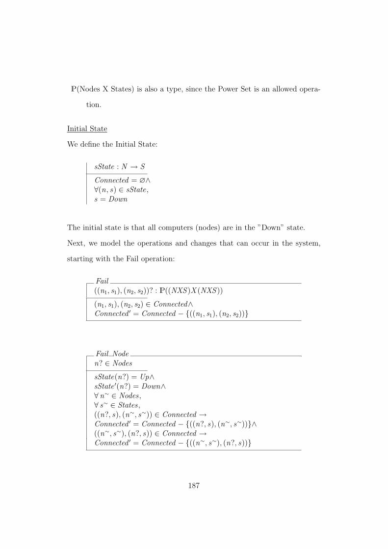
P(Nodes X States) is also a type, since the Power Set is an allowed opera-
tion.
Initial State
We define the Initial State:
sState : N → S
Connected = ∅∧∀(n, s) ∈ sState,
s = Down
The initial state is that all computers (nodes) are in the ”Down” state.
Next, we model the operations and changes that can occur in the system,
starting with the Fail operation:
Fail((n1, s1), (n2, s2))? : P((NXS )X (NXS ))
(n1, s1), (n2, s2) ∈ Connected∧Connected ′ = Connected − {((n1, s1), (n2, s2))}
Fail Noden? ∈ Nodes
sState(n?) = Up∧sState ′(n?) = Down∧∀ n∼ ∈ Nodes ,∀ s∼ ∈ States ,((n?, s), (n∼, s∼)) ∈ Connected →Connected ′ = Connected − {((n?, s), (n∼, s∼))}∧((n∼, s∼), (n?, s)) ∈ Connected →Connected ′ = Connected − {((n∼, s∼), (n?, s))}
187
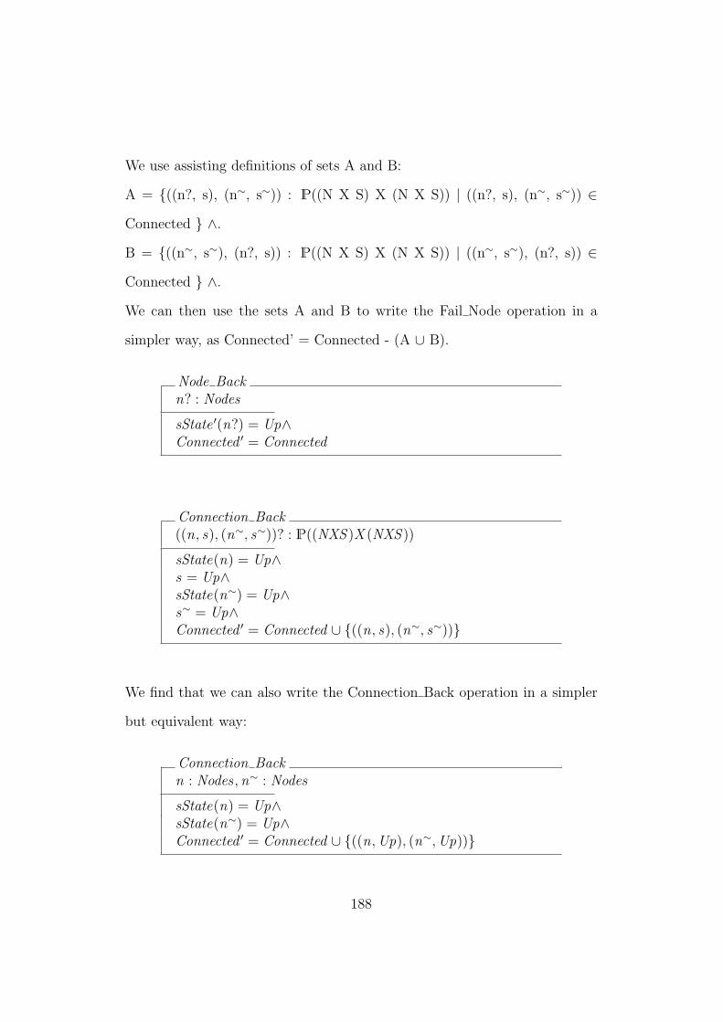
We use assisting definitions of sets A and B:
A = {((n?, s), (n∼, s∼)) : P((N X S) X (N X S)) | ((n?, s), (n∼, s∼)) ∈
Connected } ∧.
B = {((n∼, s∼), (n?, s)) : P((N X S) X (N X S)) | ((n∼, s∼), (n?, s)) ∈
Connected } ∧.
We can then use the sets A and B to write the Fail Node operation in a
simpler way, as Connected’ = Connected - (A ∪ B).
Node Backn? : Nodes
sState ′(n?) = Up∧Connected ′ = Connected
Connection Back((n, s), (n∼, s∼))? : P((NXS )X (NXS ))
sState(n) = Up∧s = Up∧sState(n∼) = Up∧s∼ = Up∧Connected ′ = Connected ∪ {((n, s), (n∼, s∼))}
We find that we can also write the Connection Back operation in a simpler
but equivalent way:
Connection Backn : Nodes , n∼ : Nodes
sState(n) = Up∧sState(n∼) = Up∧Connected ′ = Connected ∪ {((n,Up), (n∼,Up))}
188

So far, we discussed a communication group modeled by a directed graph
type; that is, there is an explicit direction between the nodes defining a
source node and a target node.
In the following definitions we define the equivalent definitions for a non-
directed graph model of the communication group example.
Connected : P(P(Nodes))
∀ x ∈ Connected ,
| x |= 2∧∀ y ∈ x ,
sState(y) = Up
The Initial State is defined as:
∀ n ∈ Nodes, sState(n) = Down ∧ Connected = ∅.
Down Noden? : Nodes
sState(n?) = Up∧sState ′(n?) = Down∧∀{n?, n} : P(P(Nodes)){n?, n} ∈ Connected → {n?, n} 6∈ Connected ′
Up Noden? : Nodes
sState ′(n?) = Up∧Connected ′ = Connected
189

Up Connectionn1? : Nodes , n2? : Nodes
sState(n1?) = Up∧sState(n2?) = Up∧Connected ′ = Connected ...
Down Connectionn1? : Nodes , n2? : Nodes
sState(n1?) = Up∧sState(n2?) = Up∧Connected ′ = Connected − ...
21.2 Functional Coverage
Definition
Functional coverage is a method that systematically creates functional cover-
age models, each containing a large sets of verification (coverage) tasks, and
monitors the testing to see if these tasks were performed.
Functional coverage models come in many flavors:
• Models can cover the inputs and outputs of a program.
• Models can model the internal state of the program (e.g., values of
variables).
• Snapshot models that model the state of the program at a certain point
in time.
• Temporal models, dealing with scenarios.
190

• Usually, functional coverage models involve modeling several properties
in parallel.
• Models can be based on the specifications of the application (Black-
Box).
• Models can also be derived from implementation (WhiteBox).
The first and most important step in the functional coverage process is de-
ciding what to cover or, more precisely, on what coverage models to measure
coverage. To make coverage successful and use it to influence the testing
process, it is important to create good coverage models, using the following
guidelines:
1. It is important to choose coverage models for areas which the user
thinks are risky or error prone.
2. The size of the model should be chosen in accordance with the testing
resources. The model size (number of tasks) should not be too large,
making it impossible to cover the model, given the testing time and
resources available.
191

22 Exercise - Functional Coverage Models
In this exercise we begin with an example of analyzing a system for extracting
a functional coverage model.
Example
Consider the following system (see Figure 5).
Figure 5: Sample front end/back end System
The system includes a front end and a back end, each with two components
termed Software and OS.
Exercise
Analyze the system in terms of bad-path testing.
Bad-path testing relates to the options that can go wrong, and how the
system handles recovery from these errors. Figure 6 displays the transactions
192
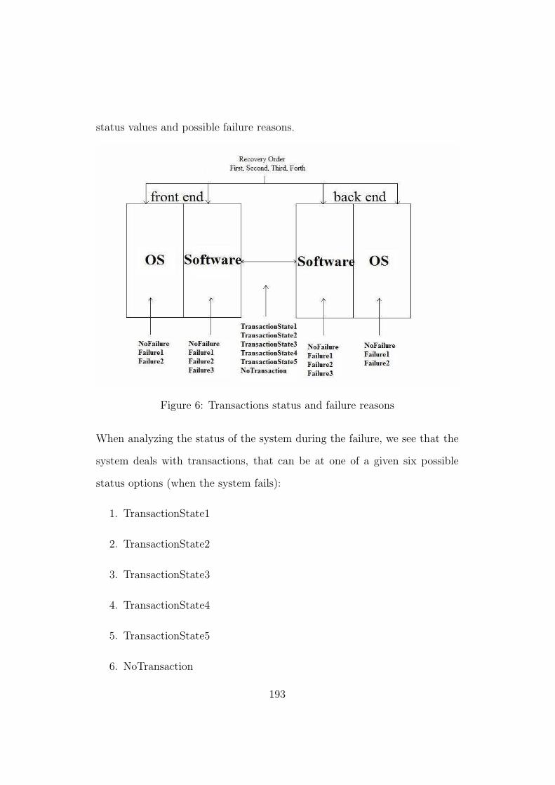
status values and possible failure reasons.
Figure 6: Transactions status and failure reasons
When analyzing the status of the system during the failure, we see that the
system deals with transactions, that can be at one of a given six possible
status options (when the system fails):
1. TransactionState1
2. TransactionState2
3. TransactionState3
4. TransactionState4
5. TransactionState5
6. NoTransaction
193

Each of the four components can fail due to a given predefined reason. The
OS component can fail due to one of three given reasons:
1. NoFailure
2. Failure1
3. Failure2
The Software component can fail due to one of four given reasons:
1. NoFailure
2. Failure1
3. Failure2
4. Failure3
Several components can fail, each for any given reason. Each of the failing
components then needs to be brought back up (only the failing components).
The order in which they are brought up is also important.
In testing, we aim to test all the possible options. When we try to test all
possible options of all failure types, all the order types, and so on, we reach a
very large number. When considering that setting up, analyzing, and testing
each option takes time, we conclude that an exponential time frame is needed
for testing.
To overcome the time obstacle, we relax some of the constraints. For in-
stance, we decide to cover each pair of test options. Figure 7 displays the
combinatorial test design report results.
194

Figure 7: Combinatorial test design report
195

23 Exercise - FoCuS Models
In this exercise we learn how to define attributes and constraints in FoCuS.
23.1 Defining Attributes
• frontSoftware = {”Failure1”, ”Failure2”, ”Failure3”, ”NotFailed”}.
• backSoftware = {”Failure1”, ”Failure2”, ”Failure3”, ”NotFailed”}.
• frontOS = {”Failure1”, ”Failure2”, ”NotFailed”}.
• backOS = {”Failure1”, ”Failure2”, ”NotFailed”}.
• recoverFirst = {”frontSoftware”, ”backSoftware”, ”frontOS”, ”backOS”,
”none”}.
• recoverSecond = {”frontSoftware”, ”backSoftware”, ”frontOS”, ”backOS”,
”none”}.
• recoverThird = {”frontSoftware”, ”backSoftware”, ”frontOS”, ”backOS”,
”none”}.
• recoverFourth = {”frontSoftware”, ”backSoftware”, ”frontOS”, ”backOS”,
”none”}.
23.2 Defining Constraints
• No Failure Constraint: frontSoftware.equals(”NotFailed”) && back-
Software.equals(”NotFailed”) && frontOS.equals(”NotFailed”) && backOS.equals(”NotFailed”).
196

• Can’t Restart a Not Killed Component Constraint: frontSoftware.equals(”NotFailed”)
&& (recoverFirst.equals(”frontSoftware”) || recoverSecond.equals(”frontSoftware”)
|| recoverThird.equals(”frontSoftware”) || recoverFourth.equals(”frontSoftware”)).
• Another Can’t Restart a Not Killed Component Constraint: backSoft-
ware.equals(”NotFailed”) && (recoverFirst.equals(”backSoftware”) ||
recoverSecond.equals(”backSoftware”) || recoverThird.equals(”backSoftware”)
|| recoverFourth.equals(”backSoftware”)).
• Another Can’t Restart a Not Killed Component Constraint: fron-
tOS.equals(”NotFailed”) && (recoverFirst.equals(”frontOS”) || recov-
erSecond.equals(”frontOS”) || recoverThird.equals(”frontOS”) || recov-
erFourth.equals(”frontOS”)).
• Another Can’t Restart a Not Killed Component Constraint: backOS.equals(”NotFailed”)
&& (recoverFirst.equals(”backOS”) || recoverSecond.equals(”backOS”)
|| recoverThird.equals(”backOS”) || recoverFourth.equals(”backOS”)).
• Can’t Restart A Duplicate Component Constraint: recoverFirst.equals(recoverSecond)
|| recoverFirst.equals(recoverThird) || recoverFirst.equals(recoverFourth).
• Another Can’t Restart A Duplicate Component Constraint: !(recover-
Second.equals(”none”)) && (recoverSecond.equals(recoverFirst) || re-
coverSecond.equals(recoverThird) || recoverSecond.equals(recoverFourth)).
• Another Can’t Restart A Duplicate Component Constraint: !(recover-
Third.equals(”none”)) && (recoverThird.equals(recoverFirst) || recover-
Third.equals(recoverSecond) || recoverThird.equals(recoverFourth)).
197

• Another Can’t Restart A Duplicate Component Constraint: !(recov-
erFourth.equals(”none”)) && (recoverFourth.equals(recoverFirst) || re-
coverFourth.equals(recoverSecond) || recoverFourth.equals(recoverThird)).
• Duplicate ”None” permutations Constraints: recoverSecond.equals(”none”)
&& !(recoverThird.equals(”none”)).
• Another Duplicate ”None” permutations Constraints: recoverThird.equals(”none”)
&& !(recoverFourth.equals(”none”)).
• ”none” - 2 NotFailed - Constraints: ((frontSoftware.equals(”NotFailed”))
&& (backSoftware.equals(”NotFailed”)) && !(frontOS.equals(”NotFailed”))
&& !(backOS.equals(”NotFailed”))) && (recoverSecond.equals(”none”)).
• Another ”none” - 2 NotFailed - Constraints: ((frontSoftware.equals(”NotFailed”))
&& !(backSoftware.equals(”NotFailed”)) && (frontOS.equals(”NotFailed”))
&& !(backOS.equals(”NotFailed”))) && (recoverSecond.equals(”none”)).
• Another ”none” - 2 NotFailed - Constraints: ((frontSoftware.equals(”NotFailed”))
&& !(backSoftware.equals(”NotFailed”)) && !(frontOS.equals(”NotFailed”))
&& (backOS.equals(”NotFailed”))) && (recoverSecond.equals(”none”)).
• Another ”none” - 2 NotFailed - Constraints: (!(frontSoftware.equals(”NotFailed”))
&& (backSoftware.equals(”NotFailed”)) && (frontOS.equals(”NotFailed”))
&& !(backOS.equals(”NotFailed”))) && (recoverSecond.equals(”none”)).
• Another ”none” - 2 NotFailed - Constraints: (!(frontSoftware.equals(”NotFailed”))
&& (backSoftware.equals(”NotFailed”)) && !(frontOS.equals(”NotFailed”))
&& (backOS.equals(”NotFailed”))) && (recoverSecond.equals(”none”)).
198
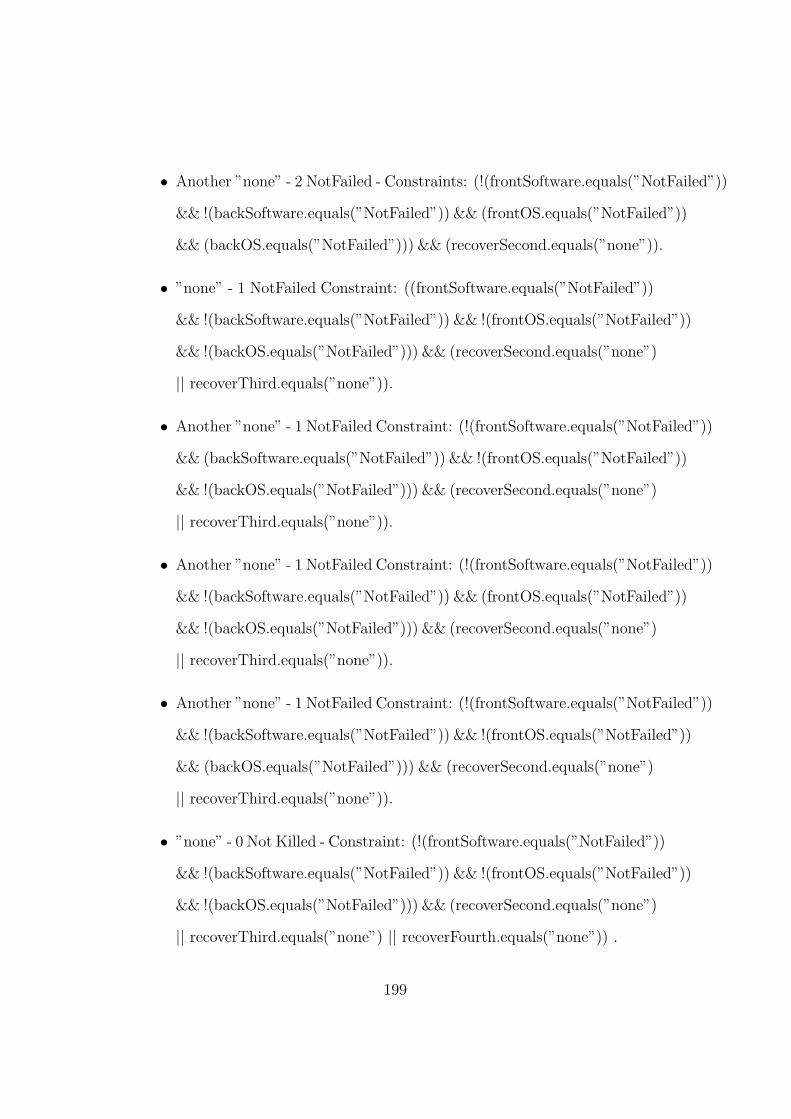
• Another ”none” - 2 NotFailed - Constraints: (!(frontSoftware.equals(”NotFailed”))
&& !(backSoftware.equals(”NotFailed”)) && (frontOS.equals(”NotFailed”))
&& (backOS.equals(”NotFailed”))) && (recoverSecond.equals(”none”)).
• ”none” - 1 NotFailed Constraint: ((frontSoftware.equals(”NotFailed”))
&& !(backSoftware.equals(”NotFailed”)) && !(frontOS.equals(”NotFailed”))
&& !(backOS.equals(”NotFailed”))) && (recoverSecond.equals(”none”)
|| recoverThird.equals(”none”)).
• Another ”none” - 1 NotFailed Constraint: (!(frontSoftware.equals(”NotFailed”))
&& (backSoftware.equals(”NotFailed”)) && !(frontOS.equals(”NotFailed”))
&& !(backOS.equals(”NotFailed”))) && (recoverSecond.equals(”none”)
|| recoverThird.equals(”none”)).
• Another ”none” - 1 NotFailed Constraint: (!(frontSoftware.equals(”NotFailed”))
&& !(backSoftware.equals(”NotFailed”)) && (frontOS.equals(”NotFailed”))
&& !(backOS.equals(”NotFailed”))) && (recoverSecond.equals(”none”)
|| recoverThird.equals(”none”)).
• Another ”none” - 1 NotFailed Constraint: (!(frontSoftware.equals(”NotFailed”))
&& !(backSoftware.equals(”NotFailed”)) && !(frontOS.equals(”NotFailed”))
&& (backOS.equals(”NotFailed”))) && (recoverSecond.equals(”none”)
|| recoverThird.equals(”none”)).
• ”none” - 0 Not Killed - Constraint: (!(frontSoftware.equals(”NotFailed”))
&& !(backSoftware.equals(”NotFailed”)) && !(frontOS.equals(”NotFailed”))
&& !(backOS.equals(”NotFailed”))) && (recoverSecond.equals(”none”)
|| recoverThird.equals(”none”) || recoverFourth.equals(”none”)) .
199

24 Exercise - Home Exercise #2
In this exercise we discuss Home Exercise #2 on FoCuS and functional cover-
age, including the uses of the cartesian product and combinatorial test design
reports in FoCuS.
Example
Consider a system that includes a Client and a Server. On each (Client/Server)
there’s a communication table. The table can be in a corrupted state or a
non-corrupted state. On each system (Client/Server), the communication ta-
ble can be in a state of being copied to the disk, or not. Also, on each system
(Client/Server), the communication table can be in a state of handling IO
operations, or not. And finally, on each system (Client/Server), there could
be a correction operation already running in parallel, or not.
A correction operation can be activated on the Client or the Server. The
purpose of the correction operation is to override a corrupted communica-
tion table with a non-corrupted table. The correction operation performs
the correction only if possible; for instance, if the table on the Server is cor-
rupted, and the table on the Client it is not corrupted, the table from the
Client can be used to override the corrupted table on the Server. But if both
tables are corrupted, a correction cannot be performed.
Between the Client and Server are active transactions. Each transaction can
be in one of five states, defined as Initiate, Rollback, Commit, Doubt, and
None. The case in which no transaction is communicated between the Client
and Server (state: None) is not interesting. On the other hand, we are able
to generate 50 transactions in parallel in each possible state of Client and
200

Server, in any transaction state we define.
When activating the correction operation, we would like to receive one of the
following results:
• Successfully Corrected.
• Correction Already In Progress.
• Try Later (IO or Copy in progress on either Client or Server).
• Not Corrected (both copies are corrupted).
• Nothing to do (both copies are not corrupted).
Exercises
1. Define an INPUT/OUTPUT model in FoCuS.
2. Define a CTD model in which each pair of options of IO state and table
copied to disk state are covered at least once.
201

25 Exercise - Home Exercise #3
In this exercise we cover questions towards Home Exercise #3 and summarize
the course (going over what we did in the lecture).
Exercise
Given A ⊆ B ⊆ C, prove that A ∪ B = B ∩ C.
Remark: why do we use this type of theorem proofing? Because if we make
it just a bit more formal, a computer could read and analyze it.
Proof
When we try to picture a diagram of the groups, we realize that since A ⊆
B ⊆ C, then A ∪ B = B and B ∩ C = B, which when combined imply that
A ∪ B = B = B ∩ C.
To prove that A ∪ B = B ∩ C, we actually need to prove two claims:
• A ∪ B = B.
• B = B ∩ C.
Claim #1: A ∪ B = B.
(Later, to complete the proof, we will also define and prove the complemen-
tary Claim #2 B = B ∩ C).
Usually when we need to prove that there is an equality between two expres-
sions, we use bi-directional subsetting, that is, we prove (Claim #1a): A ∪
B ⊆ B, and then (Claim #1b): B ⊆ A ∪ B. If we prove the two, then we
can conclude that A ∪ B = B.
How do we prove Claim #1a: A ∪ B ⊆ B?
We select any member of A ∪ B and show that this member must also be a
202

member of B.
Starting with a member x ∈ A ∪ B, by the definition of the union ∪ operator,
it implies that (x ∈ A) ∪ (x ∈ B).
Using the definition of subset ⊆, (x ∈ A) ∧ (A ⊆ B) ⇒ (x ∈ B).
Starting with (x ∈ A), we derive that (x ∈ B), denoted in formal writing as
(x ∈ A) → (x ∈ B).
From ((x ∈ A) ∨ (x ∈ B)) we derive that (x ∈ B).
We start with (x ∈ A ∪ B) and show that we can derive (x ∈ B) from (x ∈
A), and we also know that (x ∈ A) ∨ (x in B), so how do we derive that (x
∈ B)?
If we mark p ≡ (x ∈ A) and we mark q ≡ (x ∈ B), we can say that
[((x ∈ A) ∨ (x ∈ B)) ∧ ((x ∈ A) → (x ∈ B))] → (x ∈ B) ∨ (x ∈ B) is like
saying that
[(p ∨ q) ∧ (p → q)] → q ∨ q.
From q ∨ q to derive q we use a truth table (see Table 19).
Table 19: Derive Truth Tableq q ∨ q q q → q ∨ qT T T TF F F T
The same method can be used to prove that [(p ∨ q) ∧ (p → q)] → q ∨ q
(see Table 20).
This method enables us to conclude that (x ∈ B) from (x ∈ A ∪ B), which
is what we wanted to prove in Claim #1a.
Claim #1b is that for any member (x ∈ B), we derive that (x ∈ A ∪ B).
Proof of Claim #1b
203

Table 20: Truth Table for Proof
p q p ∨ q p → q (p ∨ q) ∧ (p → q) q ∨ q (p ∨ q) ∧ (p → q) → q ∨ qT F T F F F TF F F F F F TT T T T T T TF T T T T T T
We start with (x ∈ B). We prove that we can derive ((x ∈ B) ∨ (x ∈ A)),
which by the definition of ∪ is equivalent to x ∈ (A ∪ B).
We need to prove that we are allowed to derive ((x ∈ B) ∨ (x ∈ A)) from (x
∈ B).
Marking q as (x ∈ B) and p as (x ∈ A) we need to prove that we are allowed
to derive
q → (p ∨ q).
From q to derive p ∨ q we use a truth table (see Table 21).
Table 21: Derivation Truth Tableq p p ∨ q q → (p ∨ q)T T T TF F F TT F T TF T T T
Reminder
Truth table for → is: ”if then” relationship: p → q (see Table 22).
Table 22: If Then Truth Tablep q p → qT T TT F FF T TF F T
204

This completes the proof of Claim #1b, and along with Claim #1a, it com-
pletes the proof of Claim #1.
Proof of Claim #2 is very similar.
205

26 Exercise - Defining a Library Example
In this exercise we cover
• Function Types.
• Questions towards Home Exercise #3 and the final test.
• A summary of the course (recalling what we did in the lectures).
26.1 Functions
Definition: A function is a relation that maps at most one single member in
the destination set for each member in the source set.
Example: IsIn == {London 7→ England, Oxford 7→ England, Bonn 7→ Ger-
many, Paris 7→ France}.
The function IsIn is of type Cities → Countries, and it maps certain cities
to the countries in which they reside.
dom(IsIn) = {London, Oxford, Bonn, Paris}.
ran(IsIn) = {England, Germany, France}.
Formal Definition: A relation R of type X ↔ Y is a function if and only if:
∀ x : X; y, z : Y • (x 7→ y) ∈ R ∧ (x 7→ z) ∈ R ⇒ y = z.
In words this definition says that if x is mapped to y, and x is mapped to z,
then y and z must be the same member.
Partial Function
Definition: A function where the domain is a subset of the source.
We mark f : X 7→ Y.
dom(f) ⊂ X.
206

Example: The function IsIn is a partial function because we see that dom(IsIn)
is a subset (not equal) to the source set Cities (all the cities).
Formal Definition: X 7→ Y == {R : X ↔ Y | ∀ x : X; y, z: Y ◦ x 7→ y ∈ R
∧ x 7→ z ∈ R ⇒ y = z}.
Full Function
Definition: A full function is a function whose source is equal to the source
set.
f: X → Y, where dom(f) = X.
Formal Definition: X → Y == {f : X 7→ Y | dom(f) = X}.
Exercise: Given a function that maps an age to each person, is this definition
a full function?
Solution: Yes, it defines a full function, because every person has an age.
Exercise: Is the ”IsIn” function, which maps the country to each city, a full
function?
Solution: Yes, IsIn is a full function, because every city resides in a country.
Bijective (also known as a 1-to-1) Function
Definition: A function that for every member in the destination, there is at
most one member in the source that maps to that member.
f : A � B defines a full and bijective function.
f : A 7� B defines a partial and bijective function.
Formal Definition: A 7� B == {f : A 7→ B | ∀ a1, a2 : dom(f) ◦ f(a1) = f(a2)
⇒ a1 = a2}.
A � B == {f : A → B | ∀ a1, a2 : dom(f) ◦ f(a1) = f(a2) ⇒ a1 = a2}.
Example
207

f : N � N
∀ n : N ◦ f (n) = n
Exercise: Is this function full/bijective/partial?
Solution: The function is full, because it is defined for any n. The function
is bijective, because it defines a single member in the source for any output
n, which is exactly the same n.
Exercise: Explain why (A 7� B) ∩ (A → B) = (A � B).
Surjective (also known as ”on to”) Function
Definition: A function that for every member in the destination, there is a
member in the source that maps to that member.
f : A →→ B defines a full and surjective function.
f : A 7→→ B defines a partial and surjective function.
Formal Definition: A 7→→ B == {f : A 7→ B | ran(f) = B}.
A →→ B == {f : A → B | ran(f) = B}.
Exercise: For each function, state its characteristics:
1. {0 7→ 1, 1 7→ 2}.
2. {0 7→ 1, 1 7→ 1, 2 7→ 1}.
3. ∅.
4. {0 7→ 0, 0 7→ 1, 0 7→ 2}.
5. {0 7→ 1, 1 7→ 2, 2 7→ 0}.
Answers:
1. partial, bijective.
208

2. full.
3. ?
4. not a function...
5. full, bijective, surjective.
26.2 Library Definition From Lecture #12
We aim to define books and users who can loan books. We also aim to define
the operations of loaning a book, returning a book, adding a user, removing
a user, and so on.
We define the basic types [Books] and [Users].
We add a definition of a basic type: [bookState = {Taken, notTaken}].
We aim to represent all the books that a user holds.
f : [User] → P(books).
All the taken books can then be defined as: ∪u∈User f(u).
inLib: of type P(books) defines all the books in the library as all the non-
taken books. All the books: ∪u∈User f(u) ∪ inLib = Books.
We define an invariant: [∅ = (∪u∈User f(u)) ∩ inLib] ∧ [∪u∈User f(u) ∪ inLib
= Books].
Exercise 1
Write a Z specification for a function called Return that returns a book to
the library.
Possible Solution
209

ReturnLibraryLibrary ′
book? : Booksuser? : Users
(book?, user?) ∈ TakenTaken ′ = Taken\{(book?, user?)}inLib ′ = inLibUsers ′ = Users
Exercise 2
What can be said about the state of the library after an execution of two
Taken and two Return functions?
Partial Solution
After a single Taken and Return of the same book, the library state doesn’t
change.
After a Taken and Return, the number of books on the shelves won’t change.
Exercise 3
Can anything else be said about the state of the library?
210
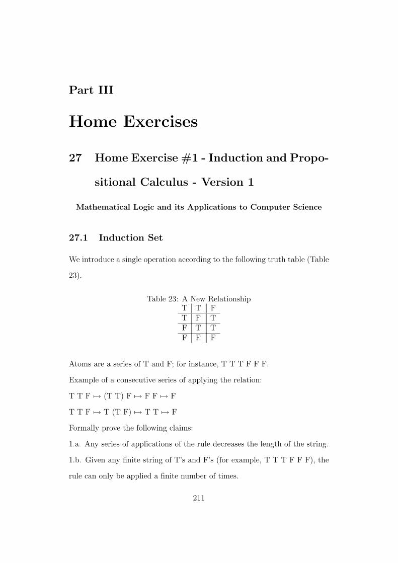
Part III
Home Exercises
27 Home Exercise #1 - Induction and Propo-
sitional Calculus - Version 1
Mathematical Logic and its Applications to Computer Science
27.1 Induction Set
We introduce a single operation according to the following truth table (Table
23).
Table 23: A New RelationshipT T FT F TF T TF F F
Atoms are a series of T and F; for instance, T T T F F F.
Example of a consecutive series of applying the relation:
T T F 7→ (T T) F 7→ F F 7→ F
T T F 7→ T (T F) 7→ T T 7→ F
Formally prove the following claims:
1.a. Any series of applications of the rule decreases the length of the string.
1.b. Given any finite string of T’s and F’s (for example, T T T F F F), the
rule can only be applied a finite number of times.
211

1.c. The length of the string when stopping is exactly 1.
1.d. The order of activation of the rule is not important as it always reaches
the same resulting string.
212
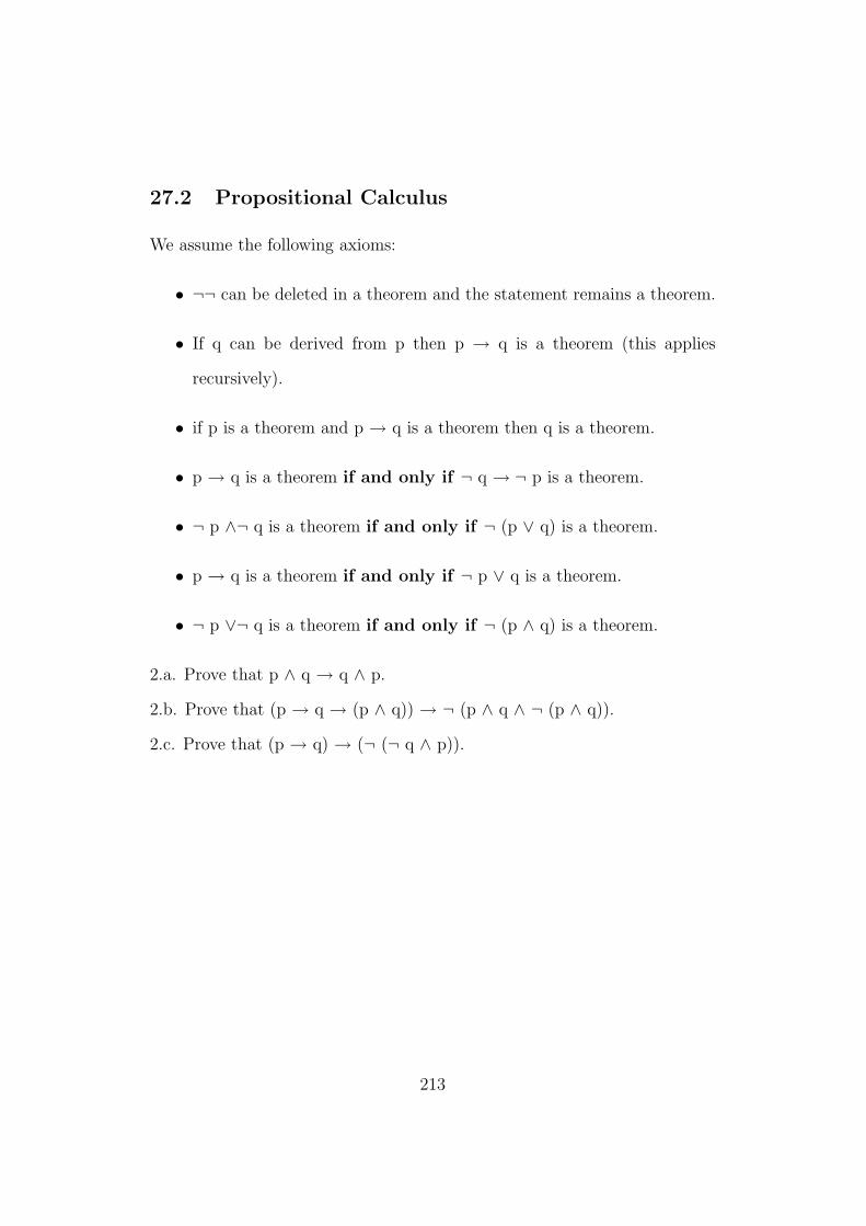
27.2 Propositional Calculus
We assume the following axioms:
• ¬¬ can be deleted in a theorem and the statement remains a theorem.
• If q can be derived from p then p → q is a theorem (this applies
recursively).
• if p is a theorem and p → q is a theorem then q is a theorem.
• p → q is a theorem if and only if ¬ q → ¬ p is a theorem.
• ¬ p ∧¬ q is a theorem if and only if ¬ (p ∨ q) is a theorem.
• p → q is a theorem if and only if ¬ p ∨ q is a theorem.
• ¬ p ∨¬ q is a theorem if and only if ¬ (p ∧ q) is a theorem.
2.a. Prove that p ∧ q → q ∧ p.
2.b. Prove that (p → q → (p ∧ q)) → ¬ (p ∧ q ∧ ¬ (p ∧ q)).
2.c. Prove that (p → q) → (¬ (¬ q ∧ p)).
213
27.3 Simple Program
For each question, define the system (as explained in Exercise # 4) and
compute I(A, P):
1. Given this program:
x = sin(t);
y = r 2 - 2;
while (x > y) {
x = x + y + 3;
}
Define the system for x and explain its purpose in words. Compute I(A, P).
2. Define for y and compute I(A, P).
3. Define the system for x and compute I(A, P) in the following program:
x = 10;
y = 100;
while (x < 50) {
x = x + y;
y = y - x;
while (y > 50) {
x = x - y;
214

y = y + x;
}
}
215

28 Home Exercise #1 - Induction and Propo-
sitional Calculus - Version 2
28.1 Induction Set
Given a single string of six digits (the Atom): ’123456’, and two operations:
1. Move the third digit to be the first digit
2. Move the sixth digit to be the fourth digit
For instance, applying the first operation on ’123456’ gives ’312456’. Apply-
ing the second operation on ’123456’ gives ’123645’.
1.a. Describe the Inductive Set that is created by the above two opera-
tions from the Atom ’123456’ (I(A, P)).
1.b. How many members are in the Inductive Set (|I(A, P)|)?
1.c. We add an additional operation, swapping the third and fourth dig-
its. For instance, applying the third operation on ’123456’ gives ’124356’.
Answer the first two questions again, including the third operation.
1.d. Is it possible to reach the string ’654321’ with just the original first
two operations? If it is possible, supply the derivation order. If not, prove
it.
216

1.e. Answer 1.d. for all three operations.
217

28.2 Propositional Calculus
We assume the following axioms:
1. ¬¬ can be added or deleted in a theorem and a theorem is obtained.
2. If p is a theorem, and q can be derived from p then p → q is a theorem
(this applies recursively).
3. If p is a theorem and p → q is a theorem then q is a theorem.
4. p → q is a theorem if and only if ¬ q → ¬ p is a theorem.
5. ¬ p ∧¬ q is a theorem if and only if ¬ (p ∨ q) is a theorem.
6. p → q is a theorem if and only if ¬ p ∨ q is a theorem.
7. ¬ p ∨¬ q is a theorem if and only if ¬ (p ∧ q) is a theorem.
Assume p is a theorem and q is a theorem.
2.a. Prove that p ∨ q → q ∨ p.
2.b. Prove that (p → q → (p ∧ q)) → (¬ ((p ∧ q) ∧ ¬ (p ∧ q))).
2.c. Prove that (p → q) → (¬ (¬ (p → q))).
218

28.3 Simple Programs and Inductive Sets
Given this program:
read a;
read d;
sum = a;
read n;
for (i = 0; i < n; i++) {
sum = sum + d;
}
1. Define an Inductive Set that characterizes the set of possible values of
the variable ’sum’, for each possible initial values of a, d, and n.
2. Prove by induction that the value of ’sum’ for the ith iteration of the
loop is a+i*d.
3. What can you deduce from Question #2 about the value of ’sum’ at
the end of the loop?
219

29 Home Exercise #2 - Functional Coverage
in FoCuS - Version 1
Mathematical Logic and its Applications to Computer Science
Home Exercise # 2 - Functional Coverage in FoCuS
Consider the following system:
System includes a Client and a Server. Each has a communication table.
The table can be in a corrupted or non-corrupted state; in a state of being
copied to the disk, or not; and in a state of handling IO operations, or not.
Each Client/Server could be already a correction operation in parallel, or
not.
A correction operation can be activated either on the Client or the Server.
The purpose of the correction operation is to override a corrupted communi-
cation table with a non-corrupted table. The correction operation performs
the correction operation if possible. For instance, if the table on the Server
is corrupted, and on the Client it is not corrupted, the table from the Client
can be used to override the corrupted table on the Server.
Between the Client and Server there are active transactions. Each transac-
tion can be in one of five states: Initiate, Rollback, Commit, Doubt, and
None. The case in which no transaction is communicated between the Client
and Server (state: None) is not interesting. On the other hand, we are able
to generate fifty transaction in parallel for each possible state of Client and
Server, in any transaction state we define.
When activating the correction operation, we would like to receive one of the
220

following results:
• Successfully Corrected
• Correction Already In Progress
• Try Later (IO or Copy in progress on either client or server)
• Not Corrected (both copies are corrupted)
• Nothing to do (both copies are not corrupted)
Exercises
1. Define an INPUT/OUTPUT model in FoCuS.
2. Define a CTD model in which each pair of options of IO state and table
copied to disk state are covered at least once.
221

30 Home Exercise #2 - Functional Coverage
in FoCuS - Version 2
Figure 8: View of Network Switching System
We would like to test a network system (see Figure 8). The system includes
1-15 racks. Each rack includes 1-15 computers (Linux boxes). Each such
Linux box has two network cards.
Each rack has an additional network component which we term ”switch”,
that chooses at any given point in time, one network card from one of the
boxes and a single rack, and provides network access for that card only. The
box whose network card receives network access is termed ”Master”. All
the other boxes are termed ”Standby”. Among the standby boxes, there
222

are priorities that dictate which box will be the next one to receive network
access.
The network system can also handle failures. We would like to test its ability
to handle a single failure in up to five seconds, and two concurrent failures
in up to fifteen seconds. The network system does not ensure a time frame
for handling more than two parallel failures.
Each Linux box has a single module, which is running. The Master has one
of the following modules running:
• ”Hello World”
• ”I am here”
• ”IO”
• ”Working Hard”
• ”Idle”
Each of the standby boxes has only one of two modules running:
• ”Hello World”
• ”I am here”
Each network failure can occur in a Linux Box (either Master or not, running
any possible module), in the switch, or between the switches of the different
racks.
1. Create a FoCuS Coverage module that describes this system. How
many legal tasks are in the Cartesian Product?
223

2. Define a CTD model in which each pair of attributes is covered at least
once.
224

31 Home Exercise #3 - Formal Specification
- Version 1
Mathematical Logic and its Applications to Computer Science
Home Exercise # 3 - Formal Specification
Define a formal specification of the possible operations ∩, ∪, and the inverse
(complementary) on the set of natural numbers so that the result of the
actions is a set with less than a thousand members, and every member in the
resulting set is an even number.
Hints
Use % for modulo
Use | x | for the size of set x
Use [N] = [1, 2, 3, 4, ...] for the natural numbers
225

32 Home Exercise #3 - Formal Specification
- Version 2
Given a system of N hosts {1, 2, 3, ..., n}, each host has a state: ”Running”
or ”Not Running”. Communication is possible between every two hosts, if
and only if both hosts are in the ”Running” state. Furthermore, the com-
munication is directed, and each host can communicate only with hosts that
have a higher number, except for the first host who can receive communica-
tion from any other host.
Example: Host 2 can communicate with host 3 (but not vice versa), and
hosts 7 and 8 can communicate with host 1 (assuming all these hosts are in
the ”Running” state).
1. Define a Formal Specification of the system, including any relation/
function needed, an initial state, and an invariant, if applicable.
2. For each type used in the definition, supply a justification for being
able to refer to this type.
3. Define operations for hosts changing states, and hosts connecting and
disconnecting from one another.
226

Part IV
References
References
[1] Herbert B. Enderton. A Mathematical Introduction to Logic. Academic
Press, second edition, 2000.
[2] Flemming Nielson, Hanne Riis Nielson, and Chris Hankin. Principles of
Program Analysis. Springer, second edition, 2005.
[3] Ben Potter, Jane Sinclair, and David Till. An Introduction to Formal
Specification and Z. Prentice Hall, second edition, 1996.
227


![[Logic] [Mathematics] - Mathematical Logic. Lecture Notes (Stephen Simpson).pdf](https://img.dokumen.tips/doc/110x75/55cf8ecd550346703b95c429/logic-mathematics-mathematical-logic-lecture-notes-stephen-simpsonpdf.jpg)