MathematicalInductionTom Davis

tomrdavis@earthlink.nethttp://www.geometer.org/mathcircles

October25,2000

1 Knocking Down Dominoes

Thenaturalnumbers,�

, is thesetof all non-negativeintegers:����� � � � � � � � � Quite often we wish to prove somemathematicalstatementaboutevery memberof

�. As a very simpleexample,

considerthefollowing problem:

Show that � �������������� � � ����� ��� ����� �� (1)

for every�����

.

In a sense,theabovestatementrepresentsa infinity of differentstatements;for every�

you careto plug in, you getadifferent“theorem”.Herearethefirst few: ����� � � � � ������������ � � � � � ������������������ � � � ������������������� � ! � � ����"andsoon. Any oneof theparticularformulasaboveis easyto prove—justaddupthenumbersontheleft andcalculatetheproducton the right andverify that they arethesame.But how do you show that thestatementis true for every�#���

? A verypowerful methodis known asmathematicalinduction,oftencalledsimply “induction”.

A nice way to think aboutinductionis asfollows. Imaginethat eachof the statementscorrespondingto a differentvalueof

�is a domino standingon end. Imaginealso that whena domino’s statementis proven, that domino is

knockeddown.

Wecanprovethestatementfor every�

if wecanshow thateverydominocanbeknockedover. If weknockthemoveroneat a time, we’ll never finish, but imaginethat we cansomehow setup the dominoesin a line andcloseenoughtogetherthatwhendominonumber$ falls over, it knocksover dominonumber$ �%� for every valueof $ . In otherwords,if dominonumber

�falls, it knocksoverdomino

�. Similarly,

�knocksover

�,�

knocksover, andsoon. If

we knockdown number�, it’s clearthatall thedominoeswill eventuallyfall.

Soa completeproof of thestatementfor everyvalueof�

canbemadein two steps:first, show thatif thestatementistruefor any givenvalue,it will betruefor thenext, andsecond,show thatit is truefor

�#���, thefirst value.

Whatfollows is a completeproof of statement1:

Supposethatthestatementhappensto betruefor a particularvalueof�

, say�#� $ . Thenwe have:������������� � � � $ � $ � $ ��� �� (2)

We would like to startfrom this, andsomehow convinceourselvesthat the statementis alsotrue for thenext value:��� $ ��� . Well, whatdoesstatement1 look likewhen��� $ ��� ? Justplug in $ ��� andsee:������������� � � � $ ��� $ ��� ��� � $ ��� � � $ ��� ��

(3)

1

Noticethat theleft handsideof equation3 is thesameastheleft handsideof equation2 exceptthatthereis anextra&('�)addedto it. Soif equation2 is true,thenwe canadd

&('�)to bothsidesof it andget:* '�)�'�+�'�, , , '�&('�- &('�) .�/ &0- &('�) .+ '�- &('�) .�/ &0- &('�) .1'�+ - &('�) .+ / - &('�) . - &('�+ .+32 (4)

showing thatif weapplya little bit of algebrato theright handsideof equation4 it is clearlyequalto- &�'#) . - &�'4+ . 5 +

— exactly what it shouldbeto make equation3 true. We have effectively shown herethat if domino&

falls, sodoesdomino&('�)

.

To completethe proof, we simply have to knock down the first domino,dominonumber0. To do so, simply plug6 / * into theoriginalequationandverify thatif youaddall theintegersfrom 0 to 0, youget* - * '�) . 5 +

.

Sometimesyou needto prove theoremsaboutall the integersbiggerthansomenumber. For example,supposeyouwould like to show thatsomestatementis truefor all polygons(seeproblem10 below, for example).In this case,thesimplestpolygonis a triangle,soif youwantto useinductionon thenumberof sides,thesmallestexamplethatyou’llbeableto look at is a polygonwith threesides.In this case,you will prove thetheoremfor thecase6 /87 andalsoshow that thecasefor 6 /9& implies thecasefor 6 /8&:'�) . Whatyou’re effectively doing is startingby knockingdown dominonumber3 insteadof dominonumber0.

2 Official Definition of Induction

Hereis a moreformal definitionof induction,but if you look closelyat it, you’ll seethatit’s just a restatementof thedominoesdefinition:

Let ; - 6 . be any statementabouta naturalnumber6 . If ; - * . is true andif you canshow that if ; - & . is true then; - &('�) . is alsotrue,then ; - 6 . is truefor every 6�<:= .

A strongerstatement(sometimescalled“stronginduction”) thatis sometimeseasierto work with is this:

Let ; - 6 . beany statementabouta naturalnumber6 . To show usingstronginductionthat ; - 6 . is truefor all 6�> *we mustdo this: If we assumethat ; - ?4. is truefor all

*A@ ?CB�&thenwecanshow that ; - & . is alsotrue.

Theonly differencebetweenthesetwo formulationsis that theformerrequiresthatyou getfrom thestatementabout&to thestatementabout

&D'�); thelatterletsyougetfrom any previousstep(or combinationof steps)to thenext one.

Noticealsothat the secondformulationseemsto leave out thepartabout ; - * . , but it really doesn’t. It requiresthatyoubeableto prove ; - * . usingno otherinformation,sincethereareno naturalnumbers6 suchthat 6 B * .Usingthesecondformulation,let’sshow thatany integergreaterthan1 canbefactoredinto aproductof primes.(Thisdoesnot show thattheprimefactorizationis unique;it only shows thatsomesuchfactorizationis possible.)

To prove it, we needto show that if all numberslessthan&

have a primefactorization,sodoes&. If&�/ *

or&4/E)

wearedone,sincethestatementof thetheoremspecificallystatesthatonly numberslargerthan1 areconsidered.If&

is prime,it is alreadya productof primefactors,sowe’re done,andif&4/�FHG

, whereF

andG

arenon-trivial factors,weknow that

F4B�&andG(B�&

. By theinductionhypothesis,bothF

andG

haveprimefactorizations,sotheproductofall theprimesthatmultiply to give

FandG

will give&, so&

alsohasaprimefactorization.

3 Recursion

In computerscience,particularly, the ideaof inductionusuallycomesup in a form known asrecursion.Recursion(sometimesknown as“divideandconquer”)is a methodthatbreaksa large(hard)probleminto partsthataresmaller,andusuallysimpler to solve. If you canshow that any problemcanbe subdivided into smallerones,andthat thesmallestproblemscanbe solved,you have a methodto solve a problemof any size. Obviously, you canprove thisusinginduction.

Here’s a simple example. Supposeyou are given the coordinatesof the verticesof a simple polygon (a polygonwhoseverticesaredistinct andwhosesidesdon’t crosseachother), andyou would like to subdivide the polygon

2

into triangles.If you canwrite a programthatbreaksany largepolygon(any polygonwith 4 or moresides)into twosmallerpolygons,thenyou know you cantriangulatethe entirething. Divide your original (big) polygoninto twosmallerones,andthenrepeatedlyapplytheprocessto thesmalleronesyouget.

Theconceptof recursionis notuniqueto computerscience—thereareplentyof purelymathematicalexamples.Here’soneof themostinterestingthatyoumaywish to play with:

Ackermann’s functionis definedasfollowson all pairsof naturalnumbers:I(J K L M1NPOQM�R�SI(J T#L K NPO�I(J TVU�S L S N L W X1TCY�KI(J T#L M1NPO�I(J TVU�S L I(J T�L M4U�S N N L�W X1T#L M#Y�KJustfor fun, try to calculate

I(J ZHL [ N. (Hint: First figureout what

I(J K L M1Nlooks like for all

M. Thenfigureout whatI(J S L M1N

lookslike, for allM

, et cetera.)

4 MakeUp Your Own Induction Problems

In mostintroductoryalgebrabookstherearea wholebunchof problemsthat look like problem1 in thenext section.They addup a bunchof similar polynomialtermson oneside,andhavea morecomplicatedpolynomialon theother.In problem1, eachtermis \ ] . Justaddthemup for \ O�K L S L ^ ^ ^ L M .Here’show to work out thetermon theright. Let’sdo:_ J M1N�O�KD` S ` [�R�S ` [D` a�R�[D` aD` ZDR�` ` ` R#M4` J M�R�S Nb` J M�R�[ N ^Work out thevalueof

_ J M1Nby handfor a few valuesof

M�O�K L S L [ L ^ ^ ^. Thefirst few

_ J M1Nvaluesare:K L c L a K L d K L [ S K L Z [ K L e f c L S [ c K ^

Now list thosein a row andtakesuccessivedifferences:0 6 30 90 210 420 756 1260

6 24 60 120 210 336 50418 36 60 90 126 168

18 24 30 36 426 6 6 6

0 0 0

Notice thatotherthanthe top line, every numberon the tableis thedifferencebetweenthe two numbersabove it totheleft andright. If all thetermsin your sumaregeneratedby a polynomial,you’ll eventuallygeta row of all zeroesasin theexampleabove. Obviously if we continued,we’d haverow afterrow of zeros.

Now look at thenon-zeronumbersdown theleft edge:K L c L S g L S g L c L K L K L ^ ^ ^

, andusingthosenumbers,calculate:_ J M1N�O�K�h M K i R�c�h M S i R�S g�h M [ i R�S g�h M a i R�c�h M Z i R�K�h M f i R�K�h M c i R�` ` ` ^ (5)

Rememberthat j k l m O9S , j k n m O�M , j k ] m O�M�J M:U#S N o [ p , j k q m O�M�J M:U#S N J M:U�[ N o a p , j k r m O�M�J M:U#S N J M:U4[ N J M:U4a N o ZHp ,andsoon.

Equation5 becomes:_ J M1N�O�K�R�c M�R S g M�J M4U�S N[ R S g M�J M4U�S N J M4U�[ Nc R c M�J M4U�S N J M4U�[ N J M4U#a N[ Z ^3

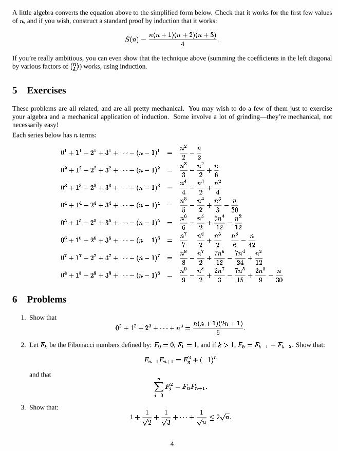
A little algebraconvertstheequationabove to thesimplifiedform below. Checkthat it worksfor thefirst few valuesof s , andif you wish,constructa standardproofby inductionthatit works:t u s1v�w s u s�x�y v u s4x�z v u s�x�{ v| }If you’re really ambitious,you canevenshow thatthetechniqueabove (summingthecoefficientsin theleft diagonalby variousfactorsof ~ � � � ) works,usinginduction.

5 Exercises

Theseproblemsareall related,andareall pretty mechanical.You may wish to do a few of themjust to exerciseyour algebraanda mechanicalapplicationof induction. Someinvolve a lot of grinding—they’re mechanical,notnecessarilyeasy!

Eachseriesbelow hass terms:� � x�y � x�z � x�{ � x�� � � x u s4��y v � w s1�z � s z� � x�y � x�z � x�{ � x�� � � x u s4��y v � w s1�{ � s1�z x s �� � x�y � x�z � x�{ � x�� � � x u s4��y v � w s0�|V� s1�z x s1�|� � x�y � x�z � x�{ � x�� � � x u s4��y v � w s1�� � s0�z x s1�{ � s{ �� � x�y � x�z � x�{ � x�� � � x u s4��y v � w s1�� � s1�z x � s0�y z � s1�y z� � x�y � x�z � x�{ � x�� � � x u s4��y v � w s1��E� s1�z x s1�z � s1�� x s| z� � x�y � x�z � x�{ � x�� � � x u s4��y v � w s1�� � s1�z x � s1�y z � � s0�z |�x s1�y z� � x�y � x�z � x�{ � x�� � � x u s4��y v � w s1�� � s1�z x z s1�{ � � s1�y � x z s1�� � s{ �6 Problems

1. Show that � � x�y � x�z � x�� � � x�s � w s u s�x�y v u z s�x�y v� }2. Let � � betheFibonaccinumbersdefinedby: �1�Dw � , � � w9y , andif ���%y , � � w�� � � � x�� � � � . Show that:� � � � � � � � w�� �� x u �Dy v �

andthat �� � � � � �� w�� � � � � � }3. Show that: y�x y� z x y� { x�� � � x y� s9� z � s }

4

4. Show that: �   ¡ ¢H  ¡ £   ¡ ¡ ¡ ¤ � ¥1¦   §%¤ ¤ ¥4¨�© ¦   ¦ ªH«5. Show that: ¬ ��¨�­ ��¨�® ��¨�¡ ¡ ¡ ¨�¯ �A°���± ² ³µ´� ª ¶b·H¸

wherethereare

¥2sin theexpressionon theleft.

6. (Chebyshev Polynomials)Define ¹bº ¤ »0¦ asfollows:¹1¼ ¤ »0¦½° ©¹ · ¤ »0¦½°Q»¹ ª ¶b· ¤ »0¦½°Q» ¹ ª ¤ »H¦�¾ ¹ ª ¿1· ¤ »0¦ ¸ À ² Áb¥#Â�à «Show that ¹ ª ¤ ��± ² ³ Ä ¦�°

³ Å Æ1¤ ¥�¨�© ¦ ij Å Æ Ä «7. Show that: ³ Å Æ ÄD¨�³ Å Æ�� ÄD¨�³ Å Æ�Ç ÄD¨�¡ ¡ ¡ ¨�³ Å Æ ¥0ÄA° ³ Å Æ4È0É ª ¶b· Ê ËÌÎÍ ³ Å Æ4È ª ËÌDͳ Å Æ4È ËÌ Í8. (Quicksort)Provethecorrectnessof thefollowing computeralgorithmto sorta list of

¥numbersinto ascending

order. Assumethattheoriginal list is Ï » ¼ ¸ » · ¸ « « « ¸ » ª ¿1· Ð «Sort(Ñ ,Ò ) whereÑ�Ó%Ò sortstheelementsfrom

» Ôto

»0Õ ¿1·. In otherwords,to sort theentirelist of

¥elements,

call Sort(

Ã,

¥). (NotethatSort(Ñ , Ñ ) sortsanemptylist.)

Hereis thealgorithm:Ö (Case1) If Ò ¾ Ñ:Ó © , do nothing.Ö (Case2) If Ò ¾ Ñ Â9© , rearrangetheelementsfrom

»HÔ ¶1·through

»0Õ ¿1·sothatthefirst slotsin thelist are

filled with numberssmallerthan

» Ô, thenput in

»HÔ, andthenall thenumberslargerthan

» Ô. (This canbe

doneby runningapointerfrom the

¤ Ò ¾#© ¦ × Ø slotdown andfrom the

¤ Ñ ¨�© ¦ × Ø slotup,swappingelementsthatareoutof order. Thenput

» Ôinto theslot betweenthetwo lists.)

After this rearrangement,supposethat

»HÔwindsup in slot Ù , whereÑ#Ó%ÙÛÚ8Ò . Now applySort(Ñ ,Ù )

andSort(Ù ¨�© , Ò ).9. (Towersof Hanoi) Supposeyou have threepostsanda stackof

¥disks,initially placedon onepostwith the

largestdiskonthebottomandeachdiskaboveit is smallerthanthediskbelow. A legalmoveinvolvestakingthetopdisk from onepostandmoving it sothatit becomesthetopdiskonanotherpost,but everymovemustplacea disk eitheron anemptypost,or on top of a disk larger thanitself. Show that for every

¥thereis a sequence

of movesthatwill terminatewith all thediskson a postdifferentfrom theoriginal one. How many movesarerequiredfor aninitial stackof

¥disks?

5

10. (Pick’sTheorem)Givenasimplepolygonin theplanewhoseverticeslie on latticepoints,show thattheareaofthepolygonis givenby Ü�Ý�Þ:ß à�á�â , whereÜ is thenumberof latticepointsentirelywithin thepolygonand Þis thenumberof latticepointsthatlie on theboundaryof thepolygon.

A simplepolygonis a closedloopof line segmentswhoseonly pointsin commonaretheendpointsof adjacentpairsof segments.In otherwords,theedgesof thepolygondonottoucheachother, exceptat thevertices,whereexactly two edgesmeet.Notethata simplepolygonneednotbeconvex.

ãEãEã�ãEãEãEã�ãEããEãEã�ãEãEãEã�ãEããEãEã�ãEãEãEã�ãEããEãEã�ãEãEãEã�ãEããEãEã�ãEãEãEã�ãEããEãEã�ãEãEãEã�ãEãä ä ä ä ä ä ä

ä ä äå å å å å å�æ æ æ æ

æ æIn the exampleabove, the triangle includes6 boundarypoints and 12 interior points, so its areashouldbe(accordingto Pick’s Theorem)â àDÝ�ç ß à(á�âAèEâ é . You cancheckthat this is right by noticingthat its areaistheareaof thesurroundingrectangle( ê(ë ì�è8é í ) lesstheareasof the threesurroundingtriangles:(5/2, 15/2,and32/2).Whenwe check,weget: é íDá�ê ß à�á�â ê ß à�á#î à ß à(è9â é .

11. (Arithmetic, Geometric,andHarmonicmeans)Let ïCèCð ñ ò ó ñ ô ó õ õ õ ó ñ öH÷ be a setof positive numbers.Wedefinethearithmetic,geometric,andharmonicmeans( ø:ù ï�ú , û�ù ï�ú , and ü#ù ï�ú , respectively) asfollows:ø:ù ï�ú½è ñ òbÝ�ñ ô�Ý�ë ë ë Ý�ñ öýû�ù ï�ú½èÿþ� ñ ò ñ ôbë ë ë ñ öü#ù ï�ú½è ââñ ò Ý âñ ô Ý�ë ë ë Ý âñ öShow that ü�ù ï�ú���û�ù ï�ú���ø:ù ï�ú õIn thesolutionsection,theactualsolutionis precededby acoupleof hints.

12. (Catalannumbers)Given ý pairsof parentheses,Let �0ö bethenumberof waysthey canbearrangedin a validmathematicalexpression.For example,if ý è�î , thereare5 waysto rearrangetheparentheses:ù ù ù ú ú ú ó ù ù ú ú ù ú ó ù ú ù ù ú ú ó ù ù ú ù ú ú ó ù ú ù ú ù ú óso ����è�ê . Let ���Dè9â . Show that: �1ö:è âý Ý�â � à ýý õHint: Show that: ��� bò è���� ��� Ý���� �1ò �1ò�Ý�ë ë ë Ý���� ��� õ

6

7 Solutions

1. If ����� we trivially have: � ����� � � � � � � � � �Assumethattheequationis truefor ����� :� �! � �! �" " " � � � ��� � � � � # � � �� � (6)

Fromthis,wewantto show that:� � � � �" " " � � � � � � �$� � � � � � � � � � � � � # � � � � � ��� � � � � � � # � � # � &% �� �Begin with Equation6 andadd � � � � � to bothsides:� � � � �" " " � � � � � � ��� ��� � � � � # � � �� � � � � � �Justdo somealgebra,andtheproof is complete:� � �" " " � � � � ��� ��� � � � � # � � � � � � � � ��� � �" " " � � � � ��� � � � � � # � � � � � � �� � � � � � � � # � � # � �% �� �

2. Part1:

First checkfor ���'� : (�) ( � ��� " #*���*� ( �+ � ,-� � + �'��,&����� �If weassumeit is truefor ����� , wehave:(/. 0 + (�. 1 + � ( �. � ,2� � . � (7)

Fromthis,we needto show thattheequalitycontinuesto hold for ���3� � . In otherwords,we needto showif we begin with Equation7 wecanshow that:(/. (/. 1 � � ( �. 1 + � ,2� � . 1 + �Since

(/. 1 � � (�. (/. 1 + , theequationabove is equivalentto:(/. � (/. (/. 1 + �!� ( �. 1 + � ,2� � . 1 + 4or to ( �. (/. (/. 1 + � ( �. 1 + � ,2� � . 1 + �Substitute

( �. from theright-hand-sideof Equation7:(/. 0 + (�. 1 + ,�� ,2� � . (/. (/. 1 + � ( �. 1 + � ,2� � . 1 + 47

or 5/6 7�8 9 5�6 :�8!;�5/6 <!=�52>6 7/8 ;�9 ?2@ < 6 7/8 ;�9 ?-@ < 6 =�5->6 7�8 Aor 5 >6 7�8 =�5 >6 7/8 BPart2:

For C =�D : EF G H E 5->G =�5->E =�D-=�5 E 5I8�=�D2J @�=�D BIf it’s truefor C =�K : 6F G H E 52>G =�5/6 5/6 7�8

(8)

wecanadd5 >6 7/8

to bothsidesof Equation8 to get:6 7/8F G H E 52>G =�5�6 5/6 7�8I;&52>6 7/8 =�5/6 7�8 9 5�6�;&5�6 7/8 <I=�5/6 7�8 5/6 7 > B3. For C ='@ we needto show that: @2L�M N @�=�M B

Assumetheequationis truefor C =�K :@!; @N M ; @N O ;�J J J ; @N K L�M N K BTo show thatit is alsotruefor C =�K-;�@ , add

@ P N K-;�@to bothsides:@!; @N M ; @N O ;�J J J ; @N K ; @N K-;�@ L�M N K-; @N K-;�@ B

If wecanshow that M N K*; @N K-;�@ L&M N K-;�@thenwe aredone.Multiply bothsidesby

N K-;�@andthensquarebothsidesto obtain:Q K�9 K-;�@ <�; Q�R K�9 K-;�@ <�;�@-L Q 9 K >I;&M K-;�@ < B

Rearrange: Q R K�9 K-;�@ <!L Q K-; O Aandsquarebothsidesagain: @ S K >!;�@ S KTL3@ S K >I;&M Q K2;&U Awhich is obviously true.

8

4. First show it is truefor V�W3X : Y W Y Z [3\ Y Z ] ^ W Y _Now assumeit is truefor V�W�` : Y Z a b�Z a c Z a a a \ Y ` ] Z [�\ \ `*d�X ] Z ] e _ (9)

If wemultiply bothsidesof Equation9 by

\ Y \ `-d�X ] ] Z , we obtain:Y Z a b�Z a a a \ Y ` ] Z \ Y `-d Y ] Z [3\ \ `-d�X ] Z ] e \ Y `-d Y ] ZIf we canshow thattheright handsideof theequationabove is largerthan

\ \ `*d Y ] Z ] e f/^ , we aredone.Noticethattheterm

\ Y `-d Y ] Z on theright handsidecanbewritten:\ Y `-d Y ] Z W \ Y `-d Y ] \ Y `-d�X ] \ Y ` ]�a a a \ `-d&g ] \ `-d Y ] ZThisconsistsof ` terms,all greaterthan `-d Y , multipliedby

\ `*d Y ] Z , so\ \ `-d�X ] Z e \ Y `-d Y ] Zihj\ \ `-d�X ] Z ] e \ `-d Y ] e \ `-d Y ] ZW \ \ `-d Y ] Z ] e \ `-d Y ] Z W \ \ `*d Y ] Z ] e f�^ _5. For V�W'X we have: k Y W YIl m n*oY p W YIl m n o/q b W Y k Y q Y W k Y _

Now assumeit’s truefor ` nestedsquareroots:r Y d�s Y d�t Y d a a a d k Y W YIl m nuoY e f�^ _If we add2 to bothsidesandtake thesquareroot, the left handsidewill now have `*d3X nestedsquareroots,andtheright handsidewill be: s Y d YIl m nuoY e f�^ _ (10)

We just needto show thatthevalueabove is equaltoYIl m nvoY e f p _(11)

We know thatfor any anglew wehave:l m n w*W s X!d

l m n Y wY _(12)

Substitute

o/q Y e f pfor w in equation12 andwecanshow theequalityof theexpressions10 and11 above.

6. (Chebyshev Polynomials)First, let’s show thattheformulaholdsfor both V�W�x and V�W'X . (For this example,wemustdo theproof for thefirst two cases,becauseto getto thecase2d&X , weneedto usetheresultfor ` andfor `*y�X .)CaseV�W�x : X�W�z�{ \ YIl m n w ] W n | } wn | } w W3X _

9

Case~��'� : �I� � � � ���/� � �I� � � � � � � � ��� �� � ��� � �I� � �!�!� � � �� � ��� � �I� � � � �Now assumethatit’s truefor ~���� and ~����*�&� , where�T��� :�/� � �I� � � � � � � � � � �-��� � �� � ����� �/� ��� � �I� � � � � � � � � � �� � ��� �Fromthedefinitionof �/� ��� � � � we thenhave:��� �/� � �I� � � � � � �I� � � � ��� � �I� � � � � ����� ��� � �I� � � � �� �I� � � � � � � � �-��� � �� � ��� � � � � � �� � ���Usethetrick that � � �'� �-��� � � � � to rewrite theright handsideof theequationaboveas:�/� ��� � �I� � � � � � �I� � � �!� � � � �-��� � � � � � � � � �-��� � � � � �� � ���� �I� � � �!� � � � �-��� � � � � � � �!� � � � �-��� � � � � � � � �*��� � �!� � ���� � ���� � � � �!� � � � �-��� � � � � � � � �-��� � �!� � ���� � ���� � � � � �-� � � �� � ��� �

7. To simplify thenotation,let’s let: � � � � � � � � ��� � � � ��� � ��� � � � � � � � ���To provethestatementfor ~��'� weneedto checkthat:� � �!� � � � � � � � � � � � � � � � � � � � � � � � �� � � � � � � � � � � ��� �Assumeit is truefor ~���� : � � � � � � � � �T� � �/� � �� � � � � ��� � � �� �Since

� � ��� � � � � � � � � � � � � � � �-��� � � , we have:� � �/� � � � � � � ��� � ��� � �� � � � � �� � � � � � �-��� � �!� � � ��� � � ��Now, usingthefactthat

� � � � �*��� � � � � � ��� � � �-��� � � � � � andthatfor any angle  , � � ���  �� �I� � �   � � �   :� � �/� � � � � � � ��� � ��� � �� � � � � �� � �I� � ��� � ��� � �� � � �!� � �/� � �� � � � ��� � � ��� � �/� � � � � � � ��� � ��� � ��¢¡ � � � � �� � �I� � �I� � �/� � �� � � � �� £� � � ��10

Now usethetrick that ¤ ¥ ¦�§ ¨ © ª « ¬I­�¤ ¥ ¦�§ § ¨*®�¯ ¬ © ª «�°�© ª « ¬ andexpandit asthesineof a sumof angles:±�² ³/´ § © ¬ ­ ¤ ¥ ¦�µ ² ³�´ ¶ ·¸¢¹ ¤ ¥ ¦Tµ ² ³/´ ¶ ·¸¢º » ¤ ·¸ ° º » ¤!µ ² ³�´ ¶ ·¸ ¤ ¥ ¦ ·¸ ®*« º » ¤Iµ ² ³/´ ¶ ·¸ ¤ ¥ ¦ ·¸ ¼¤ ¥ ¦ ·¸±�² ³/´ § © ¬!­ ¤ ¥ ¦�µ ² ³�´ ¶ ·¸¢¹ ¤ ¥ ¦�µ ² ³/´ ¶ ·¸½º » ¤ ·¸ ® º » ¤!µ ² ³/´ ¶ ·¸ ¤ ¥ ¦ ·¸ ¼¤ ¥ ¦ ·¸

±�² ³�´ § © ¬!­ ¤ ¥ ¦�µ ² ³/´ ¶ ·¸ ¤ ¥ ¦�µ ² ³ ¸ ¶ ·¸¤ ¥ ¦ ·¸8. (Quicksort)To show thatthequicksortalgorithmworks,useinduction(surprise!)First,we’ll show thatit works

for setsof sizezeroor of size1. Thosesetsarealreadysorted,sothereis nothingto do,andsincethey fall underthefirst caseof thealgorithmwhich saysto do nothing,wearein business.

If thequicksortalgorithmworks for all setsof numbersof size ¨ or smaller, thenif we startwith a list of size¨!®�¯ , sincewepick outoneelementfor comparisonsanddividetherestof thesetinto two subsets,it is obviousthateachof thesubsetshassizesmallerthanor equalto ¨ . Sincethealgorithmworkson all of those,we knowthat the full algorithmworks sincethe numberssmallerthanthe testnumberaresorted,thencomesthe testnumber, thencomesa sortedlist of all thenumberslargerthanit.

Thisalgorithmis heavily usedin therealworld. Surprisingly, thealgorithm’sperformanceis worstif theoriginalsetis alreadyin order. Canyouseewhy?

9. (Towersof Hanoi)Again,thisis aneasyinductionproof. If thereis only onediskonapost,youcanimmediatelymoveit to anotherpostandyouaredone.

If you know that it is possibleto move ¨ disksto anotherpost,thenif you initially have ¨*®�¯ disks,move thetop ¨ of themto a differentpost,andyou know thatthis is possible.Thenyou canmovethelargestdisk on thebottomto theotheremptypost,followedby a movementof the ¨ disksto thatotherpost.

This method,which canbeshown to be the fastestpossible,requires« ² °�¯ stepsto move ¨ disks. This canalsobeshown by induction—if ¨�­¾¯ , it requires« ´ °�¯2­¾¯ move. If it’s truefor stacksof sizeup to ¨ disks,thento move ¨®'¯ requires« ² °3¯ (to move the top ¨ to a differentpost)then1 (to move the bottomdisk),andfinally « ² °�¯ (to move the ¨ disksbackon top of the movedbottom). The total for ¨®'¯ disks is thus§ « ² °�¯ ¬�®�¯!®�§ « ² °�¯ ¬I­�«2¿ « ² °�¯�­�« ² ³�´ °�¯ .Theabove proof doesn’t actuallyspellout analgorithmto solve thetowersof Hanoiproblem,but hereis suchanalgorithm.You maybeinterestedin trying to show thatthefollowing methodalwaysworks:

Supposethe postsarenumbered1, 2, and3, andthe disksbegin on post1. Take the smallestdisk andmoveit every othertime. In otherwords,moves1, 3, 5, 7, et cetera,areall of the top disk. Move the top disk in acycle—firstto post2, then3, then1, then2, then3, then1, . . .Onevenmoves,maketheonly possiblemovethatdoesnot involve thesmallestdisk. Thiswill solve theproblem.

10. (Pick’s Theorem)The proof of this dependson the fact that an À -sidedpolygon, even one that is concave,canbedivided into two smallerpolygonsby connectingtwo verticestogetherso that the connectingdiagonallies completelyinsidethepolygon. This canobviously becontinueduntil theoriginal polygonis divided intotriangles.

A 4-sidedpolygon(a quadrilateral)is thussplit into two triangles;a 5-sidedpolygoninto 3 triangles,et cetera,andin general,an À -sidedpolygonis split into À�°�« triangles.

11

We aregoing to prove Pick’s theoremby inductionon thenumberof sidesof the polygon. We will startwithÁ�Â�à , sincethetheoremmakessenseonly for polygonswith threeor moresides.

If we canshow that it worksfor trianglesthenwe’ve proventhetheoremfor thecaseÁ&¾à . We thenassumethat it holdsfor all polygonswith Ä or fewer edges,andfrom that,show that it worksfor polygonswith Ä*Å�Æedges.

We’ll delaytheproof for Ä Â�à for amoment,andlook athow to do theinductionstep.Whenyour Ä�Å�Æ -sidedpolygonis split, it will besplit into two smallerpolygonsthathaveanedgein common,andthatbothhave Ä orfewer edges,soby the inductionhypothesis,Pick’s Theoremcanbeappliedto bothof themto calculatetheirareasbasedon thenumberof internalandboundarypoints. Theareaof theoriginal polygonis thesumof theareasof thesmallerones.

Supposethetwo sub-polygonsof theoriginalpolygon Ç are ÇIÈ and Ç�É , whereÇ/È hasÊ È interiorpointsand Ë2Èboundarypoints. Ç�É hasÊ É interiorand Ë�É boundarypoints.Let’salsoassumethatthecommondiagonalof theoriginalpolygonbetweenÇ/È and Ç�É containsÌ points.For concreteness,let’sassumethat Ç hasÊ interiorandË boundarypoints. ÍÎ Ç-Ï Â ÍÎ ÇIÈ Ï�Å ÍÎ Ç�É Ï Â Î Ê ÈIÅ&Ë2È Ð Ñ�Ò�Æ Ï�Å Î Ê É!Å�Ë2É Ð Ñ2Ò�Æ Ï ÓSinceany point interior to Ç/È or Ç/É is interior to Ç , andsinceÌÔÒ�Ñ of thecommonboundarypointsof ÇIÈ andÇ�É arealsointerior to Ç , Ê Â Ê ÈIÅ�Ê É!Å�ÌÕÒ�Ñ . Similar reasoninggives Ë Â Ë2ÈIÅ&Ë�É�Ò�Ñ Î ÌÔÒ�Ñ Ï/Ò�Ñ .Therefore:

Ê�Å&ËÐ Ñ�Ò�Æ Â Î Ê ÈIÅ&Ê É!Å�ÌÕÒ�Ñ Ï/Å Î Ë-ÈIÅ�Ë2É!Ò�Ñ Î ÌÔÒ�Ñ Ï/Ò�Ñ Ï Ð Ñ�Ò�ÆÂ Î Ê ÈIÅ&Ë2È Ð Ñ�Ò�Æ Ï�Å Î Ê É!Å�Ë2É Ð Ñ2Ò�Æ Ï Â ÍÎ Ç2Ï ÓThe easiestway I know to show that Pick’s Theoremworks for trianglesis to show first that it works forrectanglesthatarealignedwith thelattice,thento show thatit worksfor right trianglesalignedwith thelattice,andusingthat,weshow thatit worksfor arbitrarytriangles.

For rectangles,it’s easy. SupposetherectangleÖ is of size Á by Ì . Therewill be Ñ ÌÕÅ�Ñ Á boundarypointsand

Î ÌiÒ'Æ Ï Î Á Ò'Æ Ï interior points (convince yourself this is true with a drawing). Thus, Ë Â Ñ Ì×Å3Ñ Á ,Ê Â Î ÌÕÒ�Æ Ï Î Á Ò&Æ Ï , andtheareais Ì Á . So:Ì Á� ÍÎ Ö2Ï Â Ê2Å&Ë*Ð Ñ2Ò�Æ Â Î ÌÔÒ�Æ Ï Î Á Ò�Æ Ï�Å�ÌÔÅ Á Ò&Æ Â Ì Á ÓAny right triangle Ø canbeextendedto a rectangleby placinga copy of it on theothersideof its diagonal.IfthetrianglehassidesÌ , Á , and Ù Ì É Å Á É , its areais Ì Á Ð Ñ . If thereare Ä pointson thediagonal,thenumberof interiorpointsof thetriangleis

Î Î ÌÔÒ&Æ Ï Î Á Ò&Æ Ï/Ò�Ä Ï Ð Ñ . Thenumberof boundarypointsis ÌÔÅ Á Å�ÆIÅ�Ä .CheckPick’s formula:Ì Á Ð Ñ Â ÍÎ Ø2Ï Â Ê2Å�ËÐ Ñ�Ò�Æ ΠΠÌÕÒ�Æ Ï Î Á Ò&Æ Ï/Ò�Ä Ï Ð Ñ�Å Î ÌÔÅ Á Å�Æ�Ò�Ä Ï Ð Ñ�Ò�Æ Â Ì Á Ð Ñ ÓAny trianglethat is not a right trianglecanbesurroundedby a rectangleandits areacanbewritten astheareaof the rectangleminustheareasof at mostthreeright triangles.Theproof for this final caseis left asaneasyexercise.Themanipulationsareverysimilar to thoseshown in theproofsabove.

11. (Arithmetic,Geometric,andHarmonicmeans)

Hint: Onceyou prove that Ú Î Û ÏTÜ ÍÎ Û Ï , thenyou canshow find a relationshipbetweenthe harmonicandarithmeticmeansthatprovestheinequalitybetweenthosetwo means.

12

Hint: Prove that Ý!Þ ß�à*á'âÞ ß�à if theset ß has ã ä elements.Later, show it is true for anarbitrarynumberofelements.

Solution:

We will first show that Ý!Þ ß�à�á&âÞ ß�à (13)

if ß containsã ä values.Thiscanbedoneby induction.If å�æ�ç , thenEquation13 amountsto:è é á è éwhich is trivially true.

To seehow theinductionstepworks,just look at goingfrom å�æ�ç to å�æ'ê . We wantto show that:ë è é è ì á è éIí&è ìãïîSquarebothsides,soour problemis equivalentto showing that:è é è ì á è ì é í ã è é è ì!í&è ììðor that ç*á è ì éIñ ã è é è ì!í&è ììð æ Þ è é ñ è ì à ìð îThis lastresultis clearlytrue,sincethesquareof any numberis positive.

Soin general,supposeit’s truefor setsof size òTæ�ã ä andwe needto show it’s truefor setsof size ã òæ�ã ä ó é ,or in otherwordsshow that: ô õë è é è ì/ö ö ö è ì ÷ á è éIí�è ì!í�ö ö ö í&è ì ÷ã ò î (14)

Rewrite Equation14as:ø õë è é/ö ö ö è ÷ õë è ÷ ó é/ö ö ö è ì ÷ á è éIí�ö ö ö í&è ÷ò í è ÷ ó é!í�ö ö ö í�è ì ÷òã îIf we let è æ õë è é è ìIö ö ö è ÷ù æ õë è ÷ ó é è ÷ ó ì/ö ö ö è ì ÷ßjæ è é/í�ö ö ö í&è ÷òú æ è ÷ ó éIí�ö ö ö í&è ì ÷òandwe know that è�û ß and

ù û ú (becausetheinductionhypothesistells ussofor ò�æ3ã ä ) thenwe needtoshow that ë è ù á ß í úãüîBut we showedabovethat

ë ß ú á�Þ ß í ú à ý ã þ andwe know thatë è ù á ë ß ú sowe aredone.

But of course,not all setshavea cardinalitythatis exactlya powerof 2. Supposewe wantto show thatit’s truefor a setof cardinality ÿ , whereÿ û òTæ�ã ä .Ourset ß3æ�� è é þ è ì þ î î î þ è ��� containsÿ elements.Let� æ è éIí�è ì!í�ö ö ö í&è �ÿ î

13

If we add ��� copiesof � to the original membersof the set � , we will have a new set �� with ��� �members:�� ���� � � � � � � � � � � � ��� ��� ��� � � � � ��� � Sincewe know that "! �� #%$&'! �� # , we have:() � ��* * * � ���,+ - � $ � �/.0� �".* * * .1� �.! '�2�2# � � (15)

If we raisebothsidesof Equation15 to thepower anddo somealgebra,weget:

� � � ��* * * � �%� + - � $43 � �/.1� �".�* * * .0� �0.�! 5�6�7# � 8 � � � ��* * * � �9$43�: � '; : � ��.�* * * .1� ��<; .9: 5�6�=; : � �/.�* * * .0� ��<; 8 � � -,+ �� � � ��* * * � �9$0� + � � -,+ �0� � � : � �/.1� �".�* * * .0� �� ; � �

which is exactly whatweweretrying to prove.

Now to completethe problem,we needonly show that >6! ��#'$? "! ��# . To show this, considerthe set �� "�� @ A � � � @ A � � � � � � @ A � ��� .We know thatthegeometricmeanis lessthanthearithmeticmean,soapplythatfactto theset �� :@� � � ��* * * � � $ 3 @� � . @� � .�* * * . @� � 8� �If we invertbothsides(which will flip thedirectionof theinequality),we have thedesiredresult.

12. (Catalannumbers)We will begin by showing thatB,C D �%� B�C B,E . B,C - � B ��.�* * * . B,E B�C � (16)

To seethis, begin with the leftmostmatchedpair of parentheses.It cancontainbetweenzeroand F matchedpairsinsideit. If it contains matchedpairs,theremainingparentheseson theright containF��1 pairs.The matchedpairscanbearrangedin

B + ways,andtheremainderinB,C -,+ ways,for G��H � � � � � F . Soexpression16

holds.

Let I ! J,#/�LKM+ N E B + J + � B�E . B � J'. B � J � .�* * *O I ! J�# P � � B,E B�E .�! B � B�E . B,E B � # J'.�! B � B�E . B � B ��. B�E B � # J � .�* * *� B ��. B � J5. B�Q J � .�* * *B�E .6J O I ! J,# P � � B�E . B � J'. B � J � .�* * * � I ! J,# �and,since

B�E �9@ : J O I ! J,# P � � I ! J,#�.�@���H �Now usethequadraticformulato solve for

I ! J�# :I ! J,#"� @"R�! @%�6S J�# � T �� J � (17)

14

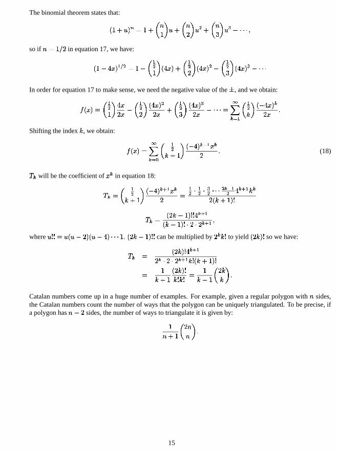
Thebinomialtheoremstatesthat:U V"W1X,Y Z'[9V"W?\ ] V ^ X'W4\ ] _ ^ X,`/W4\ ] a ^ X,b"Wc c c dsoif

] [9V e _in equation17,we have:U V�f2g h,Y i j ` [9V%f?\ i`V ^ U g h,Y�W4\ i`_ ^ U g h,Y ` f?\ i`a ^ U g h,Y b Wc c c

In orderfor equation17 to makesense,weneedthenegativevalueof the k , andweobtain:l U h�Y"[ \ i`V ^ g h_ h f \ i`_ ^ U g h,Y `_ h W \ i`a ^ U g h�Y b_ h fc c c [nmop q i\ i`r ^

U f"g h,Y p_ htsShifting theindex

r, we obtain: l U h�Y"[Lmop q,u

\ i`r W�V ^U f"g Y p v i h p_ s

(18)w p will bethecoefficientof

h pin equation18:w p [ \ i`r W�V ^

U f"g Y p v i h p_ [ i` c,i` c b` c c c ` p x i` g p v i r p_ U r WV Y yw p [ U _ r fV Y y y g p v iU r W�V Y y c _ c _ p v i dwhere

X�y y [0X�U XGf _ Y U XGf2g Y,c c c V.

U _ r f0V Y y ycanbemultipliedby

_ p r yto yield

U _ r Y ysowe have:w p [ U _ r Y y g p v i_ p c _ c _ p v i r y U r WV Y y[ V

r WVU _ r Y yr y r y [

Vr W�V \

_ rr ^ sCatalannumberscomeup in a hugenumberof examples.For example,givena regularpolygonwith

]sides,

theCatalannumberscountthenumberof waysthatthepolygoncanbeuniquelytriangulated.To beprecise,ifapolygonhas

] W _sides,thenumberof waysto triangulateit is givenby:V] W�V \ _ ]] ^�s

15

Stanford

Math

Circle

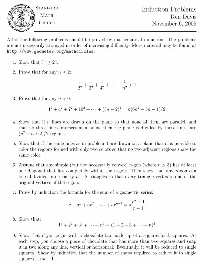
Induction ProblemsTom Davis

November 6, 2005

All of the following problems should be proved by mathematical induction. The problemsare not necessarily arranged in order of increasing difficulty. More material may be found athttp://www.geometer.org/mathcircles.

1. Show that 3n ≥ 2n.

2. Prove that for any n ≥ 2:

1

22+

1

32+

1

42+ · · ·+ 1

n2< 1.

3. Prove that for any n > 0:

12 + 42 + 72 + 102 + · · ·+ (3n− 2)2 = n(6n2 − 3n− 1)/2.

4. Show that if n lines are drawn on the plane so that none of them are parallel, andthat no three lines intersect at a point, then the plane is divided by those lines into(n2 + n + 2)/2 regions.

5. Show that if the same lines as in problem 4 are drawn on a plane that it is possible tocolor the regions formed with only two colors so that no two adjacent regions share thesame color.

6. Assume that any simple (but not necessarily convex) n-gon (where n > 3) has at leastone diagonal that lies completely within the n-gon. Then show that any n-gon canbe subdivided into exactly n − 2 triangles so that every triangle vertex is one of theoriginal vertices of the n-gon.

7. Prove by induction the formula for the sum of a geometric series:

a + ar + ar2 + · · ·+ arn−1 = arn − 1

r − 1.

8. Show that:13 + 23 + 33 + · · ·+ n3 = (1 + 2 + 3 + · · ·+ n)2.

9. Show that if you begin with a chocolate bar made up of n squares by k squares. Ateach step, you choose a piece of chocolate that has more than two squares and snapit in two along any line, vertical or horizontal. Eventually, it will be reduced to singlesquares. Show by induction that the number of snaps required to reduce it to singlesquares is nk − 1.

10. Show that for any n: √2

√3√

4 · · · (n− 1)√

n < 3.

11. Show that 3n+1 divides evenly into 23n+ 1 for all n ≥ 0.

12. Define the Fibonacci numbers F (n) as follows:

F (0) = 0

F (1) = 1

F (n) = F (n− 1) + F (n− 2), if n > 1.

Show that if a = (1 +√

5)/2 and b = (1−√

5)/2 then:

F (n) =an − bn

a− b.

13. Show that if F (n) is defined as in problem 12 and n > 0, then F (n) and F (n + 1) arerelatively prime.

14. Show that if sin x 6= 0 and n is a natural number, then:

cos x · cos 2x · cos 4x · · · cos 2n−1x =sin 2nx

2n sin x.

15. Suppose there are n identical cars on a circular track and among them there is enoughgasoline for one car to make a complete loop around the track. Show that there is onecar that can make it around the track by collecting all of the gasoline from each carthat it passes as it moves.

16. Show using induction that:n∑

k=0

(n + k

k

)1

2k= 2n.

Recursive Functions and Computability

Tom Davistomrdavis@earthlink.net

http://www.geometer.org/mathcirclesNovember 7, 2005

DRAFT!

1 What Is a Computation?

There are many ways to define what is meant by the term “computation”, but mostpeople would agree that a computation should satisfy the following characteristics:

1. A computation should be mechanical in the sense that there is a unique way toproceed at any point. (Or, at least if there is not a unique approach, then allapproaches should lead to the same result. For example, to calculate the sumx + y + z it doesn’t matter whether x + y is calculated first, or y + z. The bestsituation, of course, is if there is no ambiguity whatsoever.)

2. It must be possible to state the rules for a computation in a finite manner. Weshould not be able to list an infinte number of possible options.

3. Similarly, the size of the input and size of the output must be finite.

4. It should be clear when the process has terminated. (It may be that some com-putations never terminate, but those are usually not particularly useful, except,possibly, in a theoretical sense.)1

There are a number of different very precisely-defined mathematical schemes that sat-isfy the rules above. We can define a Turing machine that is a sort of mathematicalmodel of a computer and see what it can compute. We can define a set of primitvefunctions that are obviously computable and some rules for combining the functionsthat can obviously be performed to produce new functions and then examine what sortsof functions can be generated. We can define a formal language with syntax and gram-mar and add rules for manipulation of sentences in the language and look to see whatsorts of sentences can be “proved” from a set of sentences that are “obviously” true.Or even more simply, we can examine the sets of sentences that can be generated from

1This brings up the following consideration: suppose there is a computational method that satisfies all ofthe conditions above, but may not terminate in all cases. In other words, when you begin the computation,you know that if it terminates, it will terminate with the correct answer, but you do not know whether itwill terminate, or have any upper bound on the amount of time it may take to complete the calculation. Justbecause you have been calculating for a million years does not mean that the computation will not terminate;it may terminate on the next step. A surprising number of very useful calculations that are performed all thetime have this form.

1

various mathematically-defined grammars that generate valid sentences from a primi-tive starting point. There are other methods to approach the idea of what is meant by acomputation as well.

What is incredible is that all the methods above result in exactly the same set of com-putations, if you interpret the results of each as encodings of the others. Although atfirst glance, these computational schemes may seem wildly different, each results inexactly the same set of answers, indicating that there is something incredibly specialabout the resultant set of computations.

There is no space in this article to examine all the ideas and approaches mentioned inthe paragraphs above, but we will be able to take a look at one sort of computation;namely, computaions that can be performed by the so-called recursive functions.

The first restriction we will make is that we will consider only mathematical functionsthat take natural numbers (one or more) as inputs and yield a natural number as theoutput. In what follows, we will define the set of natural numbers2 as follows:

N = {0, 1, 2, 3, . . .}.

We want the term “computation” to include all of the obvious standard calculations:addition, subtraction, multiplication, division, factorization, integer powers, et cetera,as well as combinations of those. You may never have thought about operations likeaddition and multiplication as functions in the same way as you did f(x) in your alge-bra class, but they are. As an example, let us show how one might indicate arithmeticoperations like x · y + z · (x+ w).

One way is to replace the infix operators “+” amd “·” by functions of two variables:A(x, y) represents x + y andM(x, y) represents x · y. Then the expression x · y +z · (x+w) in the previous paragraph can be represented with the following functionalnotation:

A(M(x, y),M(z,A(x,w))).

We are of course interested in more complex operations as well. For example, supposethe function f(n) is defined to be 0 if n < 2 and the largest prime factor of n otherwise.Thus f(0) = f(1) = 0, f(2) = 2, f(3) = 3, f(4) = 2, f(5) = 5, f(6) = 3, andso on. In normal circumstances, the definition above is sufficient, but here we are alsointerested in how f(n) might be computed, given n. The expression “largest primefactor of n” really doesn’t tell us a mechanical way to calculate that number.

The fact that we restrict ourselves to the consideration of only functions of the naturalnumbers is hardly a restriction at all. For example, every computer program falls intothis category, since all the inputs are basically converted to binary (strings of zeros andones) before the program operates on them, and the outputs are binary strings beforethe final conversion to characters or colors on the screen or whatever else is produced.We can just consider these binary input and output strings to be natural numbers so thecomputer program is just a function mapping natural numbers to natural numbers.

2Some people do not include zero as a natural number, but we will do so here.

2

Similarly, the floating-point numbers used in computer computation are only finiteapproximations of the “real” real numbers. They are saved as 32, 64, or occasionally128 bit patterns, but these could equally well be considered to be 32, 64, or 128 bitnatural numbers. To be sure, the calculation of 2.71828 + 3.14159, interpreted as apurely integer operation is a very strange one, but it can be considered to be one.

2 Some Concrete Examples

Here are some examples that will be recursive functions, although to show them to beso will require some work.

2.1 The standard arithmetic functions

• The successor function: S(x) = x+ 1.

• The constant functions: (0, 1, 2, 3, . . . ).

• Addition and multiplication: A(x, y) = x+ y andM(x, y) = x · y.

• Decrement, Subtraction, Division and Remainder: x−1, x−y, x/y and x mod y.Obviously subtraction cannot go negative, so x−y is defined to be zero if y ≥ x.Similarly, division yields the whole-number divisor and the modulus functionyields the remainder, so y · (x/y) + x mod y = x.

• Integer power: xy.

Obviously we want to be able to define combinations of the functions above so that wecan perform calculations like (x+ y)(zx−w) − y.

2.2 Recursive FunctionsRecursion: If you know what recursion is, just remember the answer.

Otherwise, locate someone who is standing closer to Douglas Hofstadterthan you are, and ask him/her what recursion is.

Andrew Plotkin

The quotation above provides a surprisingly nice image of how recursion works: Arecursive calculation is one that can be done for the smallest natural number, zero, andthe calculation for larger numbers always depends on calculations for smaller ones.

2.2.1 The Factorial Function

Probably the first recursive defintion that most people see is for the factorial function:f(n) = n! = n · (n− 1) · (n− 2) · · · 3 · 2 · 1:

3

f(n) =

{1 : if n = 0,

n · f(n− 1) : otherwise.

The recursive definition above tells us that f(0) = 1, and that to compute the value off(n) if n > 0 all you need to do is look up f(n− 1) and multiply that by n.

So to calculate 3! we see that the result is 3 multiplied by 2!, but then to get 2! you needto multiply 2 by 1!, and so on. The net result is 3 · 2 · 1 · 1 = 6. More formally:

3! = f(3) = 3 · f(2)

= 3 · 2 · f(1)

= 3 · 2 · 1 · f(0)

= 3 · 2 · 1 · 1= 6.

2.2.2 The Fibonacci Sequence

An interesting function generates the Fibonacci sequence, 1, 1, 2, 3, 5, 8, 13, 21, . . .,where the first two entries are 1 and after that, each is obtained by adding the previoustwo:

f(n) =

{1 : if n = 0 or n = 1,

f(n− 1) + f(n− 2) : otherwise.

Here is the calculation for f(5):

f(5) = f(4) + f(3)

= (f(3) + f(2)) + (f(2) + f(1))

= ((f(2) + f(1)) + (f(1) + f(0))) + ((f(1) + f(0)) + 1)

= (((f(1) + f(0)) + 1)) + (1 + 1) + ((1 + 1) + 1)

= (((1 + 1) + 1)) + (1 + 1) + ((1 + 1) + 1)

= 8.

The example above deserves a couple of comments. First, the calculation as presentedis very inefficient: the values of f(n) for the small values of n are calculated overand over again. Second, in the calculation above a number of substitutions of f(n) byf(n − 1) + f(n − 2) were made in each line. One of the ways we characterized acomputation in the first section of this article was as a sequence of operations wherethere was no question about which one was to be done first. In this case, it makes nodifference, and in addition, it would be easy to specify exactly the order in which thesubstitutions should be made. For example, we could just say that at any stage of thecalculation, the leftmost possible expansion/substitution would be done.

4

2.2.3 The Greatest Common Divisor

An extremely important function yields the greatest common divisor of two numbers.For example, gcd(12, 18) = 6, since 6 is the largest number that divides both 12 and18 evenly. There is a very nice recursive definition for the gcd function:

gcd(m,n) =

{n : if m = 0,

gcd(n mod m,m) : otherwise.

For example, to calculate gcd(29680, 17360), we proceed as follows:

gcd(29680, 17360) = gcd(17360 mod 29680, 29680) = gcd(17360, 29680)

= gcd(29680 mod 17360, 17360) = gcd(12320, 17360)

= gcd(17360 mod 12320, 12320) = gcd(5040, 12320)

= gcd(12320 mod 5040, 5040) = gcd(2240, 5040)

= gcd(5040 mod 2240, 2240) = gcd(560, 2240)

= gcd(2240 mod 560, 560) = gcd(0, 560)

= 560.

The result, 560 is correct, since 29680 = 53 · 560 and 17360 = 31 · 560, and 53 and31 are obviously relatively prime. Notice that the first application of recursion simplyreverses the inputs which guarantees that afterwards the first parameter will be smallerthan the second. After that, the recursion guarantees that each successive applicationhas smaller values for the first parameter, and so it will eventually get to zero. Finally,it is not hard to show that at every stage of the calculation, the remaining numbers havethe same greatest common divisor as the previous pair of numbers.

2.2.4 Some Simple Recursive Functions

The examples above are all fairly famous; let us now consider some very simple recur-sive functions. These examples show that even the arithmetic operations like additionand multiplication that we consider to be “primitive” can in fact be defined in terms ofthe even more primitive operation, successor.

The successor function: S(n) = n + 1 yields the next larger number above n. Withthe successor function defined, we can define the addition functionA(m,n) = m+ nrecursively as follows:

A(m,n) =

{n : if m = 0,

A(k,S(n)) : if m = S(k).

The definition above basically amounts to saying that if you add zero to a number, itremains the same, and if you add m and n, that’s the same as addingm− 1 and n+ 1.Eventually the repeated subtractions of 1 fromm will get it down to zero, and we knowhow to add zero to any number.

5

A slightly different method can be used to define multiplication:M(m,n) = m · n, interms of addition: It’s easy to multiply by zero, and to multiplym by n amounts to thesame thing as multiplying m− 1 by n and adding n:

M(m,n) =

{0 : if m = 0,

A(n,M(k, n)) : if m = S(k).

Exponentiation follows the same pattern as multiplication.

These examples show that we really need nothing more than the successor functionto define the rest of the standard arithmetic functions. We will now go back to thebeginning, and give a very formal defintion of what is meant by a recursive function.

3 Recursive Functions: Informal and Formal Defini-tions

One way to build up a class of functions is to begin with a tiny set of relatively simplefunctions and to build additional functions based on combinations of the simpler ones.Then more functions are built upon those and so on. As a simple, concrete example,let’s consider the primitive recursive functions.

The general strategy will be this: we will define the set by giving a set of functions thatbelong to it, and then we will give two rules that will allow us to build more functionsfrom functions that are already in the set. Of course once you add those functions tothe set, it may be possible to apply the rules for building more functions to those andthereby obtain even more functions, and so on. If this process: beginning with a fewfunctions and then applying the function-building rules to all of them and adding thenewly-constructed functions to the set, is repeated forever, the resulting set will containall the primitive recursive functions.

We will choose the initial functions to be functions that are “obviously” easy to com-pute: it should be obvious that any human or computer should be able to make thosecomputations. The rules for building functions should also produce functions that areobviously computable. In other words, they should have the form so that if you areconvinced that the component functions are computable, it should be obvious to youthat the resulting functions will also be.

Later, when we build the set of so-called “general recursive functions”, we will useexactly the same strategy. The only difference will be that in addition to the initialfunctions and the rules for primitive recursion, we will add a single additional function-building rule.

3.1 An Informal Description

In the following section (3.2) we will give a totally formal description of the primitiverecursive functions, but it’s easy to get lost in the forest of subscripts. In this section,

6

we’ll give an intuitive description of what we’re trying to do, and then when you readthe formal definitions in the next section, it should be easy to understand them, basedon the simpler examples we present here.

Every function will take some number of natural numbers as inputs and will return anatural number as an output.

3.1.1 The Initial Functions

There will be three types of functions that we’ll initally add to the set, before we tryto make more functions from our function-generating rules. The first type consists ofonly a single function, the successor function: S(n) = n + 1. It takes a single naturalnumber as an input, adds 1 to it, and returns the result. Hopefully, most people willagree that the successor function is computable for any natural number input.

The other two types consist of an infinite number of functions, but again, hopefullymost people would agree that all of them are computable. The first type consists ofall the functions that return zero, no matter what the inputs are. This is an infinite setof functions, since we would like to include functions of 1, 2, 3, . . . variables. Now inpractical use, it’s hard to imagine a function that takes a billion (or a google) of naturalnumbers as inputs, but just to be on the safe side, we’ll include all of them. But thecomputation is quite simple: ignore all the inputs and return zero! Here’s what the listwould look like:

z1(x) = 0z2(x, y) = 0z3(x, y, z) = 0z4(x, y, z, w) = 0· · ·

The second type is essentially a doubly-infinite list of functions, but again, they are allquite simple. Each one returns a particular input with no computation done on it. Sowhat we add is a series of functions like this:

p11(x) = xp12(x, y) = x p22(x, y) = yp13(x, y, z) = x p23(x, y, z) = y p33(x, y, z) = zp14(x, y, z, w) = x p24(x, y, z, w) = y p34(x, y, z, w) = z p44(x, y, z, w) = w· · ·

The idea is simple: we need a set of functions for every possible number of inputsthat simply return each of the possible inputs. Thus we will need a million differentfunctions that take one million inputs: one that returns the first, one that returns thesecond, and so on. Again, most people would agree that, in principle, all of thesefunctions are computable. Note that we only talk about functions with a finite numberof inputs, but of every finite size. The second subscript that is part of the functionnames indicates how many parameters it takes, and the first one tells which of thoseparameters will be returned.

7

These are called the “projection functions”.

What is truly amazing, is that the three function types above: the successor function,the functions that return zero, no matter what, and the functions that simply returnone of their inputs, is all that we need to construct almost any function taking naturalnumbers as input and returning a natural number that you can imagine.

3.1.2 Composition: The First Construction Method

The idea is simple: if you know how to compute some functions, you should be able touse the outputs of those functions as inputs to other functions. In real analysis, you’veseen expressions like sin(x2) which essentially takes the value x and feeds it to thesquaring function to obtain x2. Then that value is provided as input to the sin functionwhich returns its value.

The formal definition in section 3.2 may seem like an overly-complicated way to ex-press the idea of composition, but it results from the fact that we need to be able to dothis sort of composition of functions with different numbers of inputs. In other words,if f(x, y), g(x, y) and h(x, y) are three functions that we know how to compute, andF (x, y, z) is another, then we should be able to compute a new function G(x, y) de-fined as follows:

G(x, y) = F (f(x, y), g(x, y), h(x, y)).

In other words, G takes two input values and inserts those two into f , g and h, whichyields three output values. These are then used as the three inputs that F requires.

In the definitons, we will require that each of the functions like f , g and h have thesame number of parameters. This might appear to be a problem, since you can certainlyimagine wanting to do something like this: f(x, y) is a function with two inputs, butg(x) and h(x) only take a single parameter, but we’d like to define G as follows:

G(x, y) = F (f(x, y), g(x), h(y)).

This is not really a problem, since if we need to do something like this, we can definenew functions g′(x, y) = g(x) and h′(x, y) = h(y). This kind of definiton can easilybe made with the projection functions illustrated in section 3.1.1. In fact, using thenotation in that section, we can define:

h′(x, y) = h(p22(x, y)),

where the projection function p22 snags the second parameter of a two-parameter func-tion and returns it. Note that the expression above has the correct form for functioncomposition that we’ve allowed.

Note that the projection functions will allow us to do things like permute or collapsethe order of parameters. For example, suppose that we’ve got an interesting functionalready defined: f(x, y, z) and we would like to define a new function g as follows:

g(x, y) = f(y, x, x).

8

With the projection functions, it is easy:

g(x, y) = f(p22(x, y), p12(x, y), p12(x, y)).

3.1.3 Recursion: The Second Construction Method

The examples of recursion we’ve seen in earlier sections essentially tell how a functionbehaves for the smallest input value (zero) and if the input is not zero, it tells how toobtain the result based on the value of the function with a smaller input. This processis guaranteed to terminate, since the input value cannot be smaller than zero, and whenit hits zero, we’ve given an effective way to complete the computation.

The examples are almost all simple in that they take only a single parameter, and surelywe’d like to allow for multiple parameters. To keep things simple, though, we’ll onlyallow recursion on one parameter, and this is not a real restriction. Thus we’d like ourdefinition to be something like this:

If n = 0, then f(n, x, y, . . . , z) can be computed as the value of some functiong(x, y, . . . , z), where g is some function that we know we can compute. But if n > 0,we want to have a function h that may depend not only on the values x, y, . . . , z, butalso possibly on n and on f(n − 1, x, y, . . . , z. Thus the definition of f will dependon two functions: one, g, that uses one fewer parameter than f , and tells what to do ifn = 0, and on another function h that has one more parameter than f and tells how todo the computation based on the values that f provided, but also the value of f whencalled with n− 1 as its first parameter.

Note that there’s no penalty for requiring that h have all these parameters: it can ignoreas many as it wants.

With all of the above in mind, take a look again at section 2.2.4, and see how thedefinitions of the initial functions and constrution methods could be applied to obtainfunctions like the addition and multiplication of natural numbers beginning only withthe successor function.

Now we’ll do essentially the same thing we did over again, but in a totally formal way.

3.2 Primitive Recursive Functions

The set of primitive recursive functions is the smallest set of functions that map thenatural numbers into the natural numbers and include the following functions. Thefirst three entries below name specific functions that must be included; the last two arebasically “recipes” for creating new primitve recursive functions from those that havealready been shown to be primitive recursive.

1. The successor function. S(n) = n+ 1.

2. The constant zero functions. Zk(n1, n2, . . . , nk) = 0.

9

3. The projection functions. P (k)i (n1, n2, . . . , nk) = ni, for every k ≥ i > 0.

4. Composition of functions. If f(n1, . . . , nk) is in the set and if gi(n1, . . . , nl)are in the set for 1 ≤ i ≤ k, then

h(n1, . . . , nl) = f(g1(n1, . . . , nl), . . . , gk(n1, . . . , nl))

is in the set.

5. Primitive recursion. If f(n1, . . . , nk) and g(n1, . . . , nk+2) are in the set, thenthe function h defined as follows is in the set:

h(0, n1, . . . , nk) = f(n1, . . . , nk)

h(S(n), n1, . . . , nk) = g(h(n, n1, . . . , nk), n, n1, . . . , nk)

The final recursion condition is very safe in the sense that it will always be possibleto evaluate functions so defined. The value is defined at zero, and based on that, thevalues at 1, 2, 3, . . ., are also defined, each depending upon the result of a calculationwith a smaller input.

All the so-called primitive recursive functions are thus defined for all possible inputvalues. Such functions are called “total functions”.

3.3 Examples of Primitive Recursive Functions

The vast majority of commonly-used arithmetic functions are primitive recursive. Inthis section we’ll build up a few of them. In a sense, it is easier to work with recursivefunctions in this way than with Turing machines, since once we have constructed arecursive function and studied its properties, we can just use it as it stands in the def-inition of a more complex recursive function. Embedding working Turing machinesinside other ones requires, at the least, a little more bookkeeping.

We will list a number of examples below, all in the same format. First, we’ll describeexactly the function to be implemented. Next, we will show the formal derivationusing either the functions listed above or functions that we have derived in previoussections. Finally, if warranted, we will include some discussion of the method. Sincethe definitions tend to build one on the other, in this section we have been careful togive each function a unique name that may be used in a later definition.3.

3.3.1 The constant functions

For any integers m and k, the function C(m)k (n1, . . . , nk) = m is primitive recursive.

3Although the defintions that follow may seem fairly trivial, it is a little bit tricky to get them exactlyright. They may, in fact, not be exactly right in this text. The author was a bit paranoid about getting themright, so after he wrote the first draft of this article, he wrote a computer simulator for his definitions ofprimitive recursive functions. Every one of the original definitions had at least a minor error, and some hadmajor errors!

10

C(0)k (n1, . . . , nk) = Zk(n1, . . . , nk)

C(1)k (n1, . . . , nk) = S(C(0)

k (n1, . . . , nk))

C(2)k (n1, . . . , nk) = S(C(1)

k (n1, . . . , nk))

C(3)k (n1, . . . , nk) = S(C(2)

k (n1, . . . , nk))

. . . = . . .

In other words, the successor of the functions that generate the constant output zero isthe one that has constant output 0, and so on.

3.3.2 Addition of two natural numbers

The functionA(m,n) = m+ n is primitive recursive.

A1(n1, n2, n3) = S(P(3)1 (n1, n2, n3))

A(0, n1) = P(1)1 (n1)

A(S(n), n1) = A1(A(n, n1), n, n1)

Addition is based on the idea that if you add zero to something, the result is the some-thing. To add n+ 1 to something, you can just add 1 to what you get when you add nto that same something.

To define the addition function in a completely rigorous way, we need first to define the“helper” function A1 as above. This is because in the formal definition of recursion,when we define a function with k parameters, we need a k + 1 parameter function toprovide the recursive part of the definition.

This example is quite simple: if the first parameter is zero, simply return the secondparameter. If the first parameter is the successor of n, work out the sum with n as thefirst parameter and then pass that sum, n, and the second parameter to the recursion-defining function. In this case, the recursion-defining function has no use for its secondand third parameters; it simply selects its first parameter (using P (3)

1 ) and returns thesuccessor of that.

Because the form of definition of primitve recursive functions is so rigid, we will oftenneed to use the trick above of defining one or more helper functions.

3.3.3 Doubling a natural number

The function f(x) = 2x is primitive recursive.

f(n1) = A(P(1)1 (n1),P(1)

1 (n1))

11

Obviously, since we have defined addition in the previous section, multiplying by 2is equivalent to adding a number to itself. The only thing that is slighty tricky in thedefintion above is that to exactly satisfy the form for the substitution construction, wemust pass functions of the parameter n1 rather that the parameter itself. This is trivialto do: P(1)

1 is basically the identity function.

3.3.4 Multiplication of two natural numbers

The functionM(x, y) = x · y is primitive recursive.

M1(n1, n2, n3) = A(P(3)1 (n1, n2, n3),P(3)

3 (n1, n2, n3))

M(0, n1) = Z1(n1)

M(S(n), n1) = M1(M(n, n1), n, n1)

Multiplication is defined recursively in terms of addition in much the same way thataddition is defined recursively in terms of the successor function. Multiplication byzero yields zero, and to multiply by n+ 1, you simply multiply by n and then add an-other copy. The structure of the helper function is similar to what we used for addition.Exponentiation, which we’ll do next, seems almost identical, but we’ll add one smalltrick.

3.3.5 Exponentiation of natural numbers

The function E(x, y) = xy, where 00 is defined to be 1 is primitive recursive.

E2(n1, n2, n3) = M(P(3)1 (n1, n2, n3),P(3)

3 (n1, n2, n3))

E1(0, n1) = C(1)1 (n1)

E1(S(n), n1) = E2(E1(n, n1), n, n1)

E(n1, n2) = E1(P(2)2 (n1, n2),P(2)

1 (n1, n2))

Primitive recursion is defined for all inputs, so we cannot simply make the expression00 be “undefined”. Here, we’ve arbitrarily defined it to the 1. The construction the thefunction E is very similar to multiplication except that an exponent of 0 yields 1. Thesmall trick here is that the function E1(x, y) = yx, not xy . To obtain xy we need toswap the parameters, and that’s what is done in the final line of the definition.

3.3.6 Decrement a natural number

The function ∆(x) = max(0, x − 1) is primitive recursive. (We use the Greek letterdelta (∆) since we’re reserving the symbol D to stand for subtraction. Think of it asstanding for “difference”.)

12

∆1(0, n1) = Z1(n1)

∆1(S(n), n1) = P(3)2 (∆1(n, n1), n, n1)

∆(n1) = ∆1(P(1)1 (n1),P(1)

1 (n1))

Here we would like to define the decrement function directly as a recursive function,but it only has one parameter, and every function defined using recursion according toour scheme must have at least two. We get around the problem by defining a helperfunction that has an unused parameter, and then we define decrement by plugging a“garbage” value into that second slot.

3.3.7 Subtraction of natural numbers

The functionD(x, y) = max(0, x− y) is primitive recursive.

D2(n1, n2, n3) = ∆(P(3)1 (n1, n2, n3))

D1(0, n1) = P(1)1 (n1)

D1(S(n), n1) = D2(D1(n, n1), n, n1)

D(n1, n2) = D1(P(2(2)(n1, n2),P(2)

1 (n1, n2))

The idea here is that if y is zero, then x− y is x. Otherwise, subtract y− 1 from x− 1.It’s a little tricker that it seems, and to make it work nicely, it’s easier to reverse theparameters.

3.3.8 Maximum of two natural numbers

The function max(x, y) is primitive recursive.

H1(0, n1, n2) = P(2)2 (n1, n2)

H1(S(n), n1, n2) = P(4)3 (H1(n, n1, n2), n, n1, n2)

max(n1, n2) = H1(D(n1, n2),P(2)1 (n1, n2))

The max function works by subtracting the second parameter from the first, wherethe subtraction is the usual version restricted to natural numbers. If the result is zero,then the second element is larger (or the same size). To perform the “if” statement inthe previous sentence, we need a helper function that we’ve called H1(n, n1, n2) thatbasically looks at n1 to see if it is zero. If n1 = 0, it returns n2; otherwise, n1.

13

3.3.9 Parity of a natural number

The parity function Π(x) = x mod 2 is primitive recursive.

α(0, n1, n2) = C(1)2 (n1, n2)

α(S(n), n1, n2) = Z4(α(n, n1, n2), n, n1, n2)

Π1(0, n1) = Z1(n1)

Π1(S(n), n1) = α(Π1(n, n1), n, n1)

Π(n) = Π1(P(1)1 (n),P(1)

1 )

A couple of helper functions make this work. The helper function α returns 1 if thefirst input is zero and zero otherwise. The helper function Π1(n, n1) returns zero fora n = 0, and α of itself applied to n − 1 otherwise. It is a helper function since it isrecursive and hence requires at least two parameters. The final definiton of the parityfunction Π simply invents a garbage second parameter for Π1.

3.3.10 Sum of values of a primitive recursive function

If f(n) is a primitive recursive function, then so is the following function:

σf (n) =

n∑

i=0

f(i).

σ1(n) = f(S(n))

σ2(n1, n2, n3) = σ1(P(3)2 (n1, n2, n3))

σ3(n1, n2, n3) = A(P(3)1 (n1, n2, n3), σ2(n1, n2, n3))

σ4(0, n1) = Z1(n1)

σ4(S(n), n1) = σ3(σ4(n, n1), n, n1)

σf (n) = σ4(P(1)1 (n),P(1)

1 (n))

There is nothing particularly tricky going on above—just a lot of technical problemswith numbers of parameters.

Notice that with a couple of trivial changes we can also show that finite products of thesame form of primitive recursive functions are primitive recursive:

πf (n) =

n∏

i=0

f(i).

14

3.4 Characteristic Functions (or Predicates)

If S ⊂ N, then the characteristic function of S, indicated by χS(n), is defined to be 1 ifn ∈ S and 0 if n 6∈ S.

A characteristic function can also be thought of as a predicate (a special function thatreturns either “true” or “false”) that takes inputs from the natural numbers. The usualconvention is the 1 corresponds to “true” and 0 to “false”. In this way you can imaginea function like prime(x) (or x > 7) that returns 1 (true) if and only if x is prime (orx > 7).

We will be interested, of course, in which characteristic functions (or predicates) areprimitive recursive (and later, general recursive) functions.

If characteristic functions are interpreted as predicates, then we can also investigatelogical combinations of those functions. In this way we will be able to build predicateslike prime(x) ∧ (x > 7). (The ∧ symbol signifies a logical “and” operation. In whatfollows, ∨ will indicate logical “or” and ¬ will indicate logical “not”.)

It turns out that if two predicates p and q are primitive recursive (recursive) then thepredicates p ∧ q, p ∨ q and ¬p will also be primitive recursive (recursive). This is easyto see, since if p is a predicate, then 1 − p corresponds to ¬p. Similarly, if p and qare predicates, then pq (the product of p and q) corresponds to p ∧ q. From these twofacts and from De Morgan’s law: p ∨ q = ¬((¬p) ∧ (¬q)) we can infer that p ∨ q isalso primitive recursive. (All the other common logical operations like implication,exclusive-or, nand, nor, et cetera, can be similarly constructed from ∧ and ¬).

(Notice that if we consider the functions to be characteristic functions of subsets of Ninstead of predicates, then the constructions above yield new characteristic functionscorresponding the set operations: union (∪ ↔ ∨), intersection (∩ ↔ ∧), set comple-ment (′ ↔ ¬), et cetera.)

In this section we will show how to define a few interesting primtive recursive predi-cates. The definitons below will not be so formal as they were in the previous section.Hopefully the examples there indicate how one might go about constructing the abso-lutely formal definitions. In every case, this formalization can be accomplished.

3.4.1 True and False are primitive recursive

True(x) = C(1)1 (x)

False(x) = Z1(x)

3.4.2 Finite sets

We will show that the characteristic function of any finite set is primtive recursive.This will be done by induction. The characteristic function of the empty set φ is:χφ(x) = Z1(x). We will be done if we can show that if every characteristic function

15

of a set of n− 1 elements is primitive recursive then so is the characteristic function ofany set with n elements.

We will begin by showing that the characteristic function of any singleton set is primi-tive recursive. Here is the definition of χ{0}(n):

f(0, n1) = C(1)1

f(S(n), n1) = Z3(f(n, n1), n, n1)

χ{0}(n) = f(P(1)1 (n),P(1)

1 (n))

Next, suppose that we have defined χ{0}(n), χ{1}(n), χ{2}(n), . . . , χ{k}(n) and wewish to define χ{k+1}(n). Here is how to proceed:

χ(k+1)h1

(n) = χ{k}(S(n))

χ(k+1)h (n1, n2, n3) = χ

(k+1)h1

(P(3)2 (n1, n2, n3))

f(0, n1) = Z1(n1)

f(S(n), n1) = χ(k+1)h (f(n, n1), n, n1)

χ{k+1}(n) = f(P(1)1 (n),P(1)

1 (n))

Now we have defined (by induction) the characteristic function of every singleton set.But we know from our previous discussion that if f and g are two predicates that areprimitive recursive, then f ∨ g is also primitive recursive. But f ∨ g corresponds to thepredicate of the union of the values for which both f and g are true, so we can build upa characteristic function for any finite collection of natural numbers.

3.4.3 Bounded Quantification

If P (n, n1, . . . , nk) is a primitive recursive predicate, then so is:

EFP (y, n1, . . . nk) = ∃x ((x < y) ∧ P (x, n1, . . . nk)) .

In English, this new predicate EFP (y, n1, . . . , nk) is true if there exists some value ofx < y such that P (x, n1, . . . , nk) is true. The “F ” superscript indicates a finite search.Notice that this is just a finite product:

EFP (y, n1, . . . , nk) =

y−1∏

i=0

P (i, n1, . . . , nk).

We can similarly test to see if a predicate is true for all input values less than somefixed number since:

∀x ((x < y) ∧ P (x, n1, . . . , nk)) = ¬∃x ((x < y) ∧ ¬P (x, n1, . . . , nk)) .

16

Based on this sort of operator, we can construct predicates that tell us about divisibility.To see if x divides y, just form a function like this:

x|y = ∃n ((n < y) ∧ (M(n, x) = y)) .

3.4.4 Bounded Minimization

If we have a predicate P (x, n1, . . . , nk) it is very useful to find the least value of x < ysuch that P (x, n1, . . . nk) is true. Using the results from the previous section, that isnot too hard to do.

Consider

f(y, n1, . . . nk) =∑

x<y

(∀v((v < x) ∧ ¬P (v, n1, . . . , nk))) .

This sum will basically add 1 each time there is a value of v where the predicate isfalse for it and for all smaller values. Once the predicate is true for the first time, all theother terms in the sum will add zero. Thus the sum will represent the smallest valuewhere the predicate is true for the first time.

Based upon this, we can show that division is primitive recursive:

x div y = minz<yM(y, z + 1) > x.

The mod function can be defined in terms of this:

x mod y = y − x(x div y).

Also from the fact that we can represent divisibility as a primitive recursive func-tion, the least common multiple (lcm(m,n)), greatest common divisior (gcd(m,n)),et cetera can be constructed:

lcm(m,n) = minp<mn

(m|p ∧ n|p)

gcd(m,n) = mn div (lcm(m,n))

It is also easy to define the prime(x) predicate, then a predicate that identifies the ith

prime, the number of times the ith prime divides a given number, and so on. In fact ifwe enumerate the prime numbers as p0 = 2, p1 = 3, p2 = 5 and so on, then given anynunber n, we can write primitive recursive functions that will yield k0, k1, . . . such thatn = pk0

0 pk11 . . ..

We can then define functions that yield the prime factorization of numbers, allowing usto encode multiple numbers or even strings as single numbers. See 3.5.2.

17

3.5 Functions that are not Primitive Recursive

The examples above begin to show that the number of functions that are primitve re-cursive is vast—almost every function we use in day-to-day calcutions seems to fit intothat category. But in fact, there are functions that are obviously computable that are notprimitive recursive. In this section we will show how to construct one.

The proof that there are effectively computable total functions that are not primitiverecursive is based on two ideas:

• It is possible to enumerate all of the primitive recursive functions in a logicalway such that we can say, Fi is the ith primitve recursive function, and for everyprimitive recursive function g, there exists a k such that Fk = g.

• Once we have enumerated all the primitve recursive functions, we use a diago-nalization argument to produce a function that is not in the list. Since the listincludes all the primitive recursive functions, this new function cannot be primi-tive recursive. On the other hand, we can calculate the value of this new functionfor any input, and hence it is effectively computable.

The description above glosses over some of the difficulties, and we will eventuallymake the argument completely rigorous, but first let’s see the general idea.

Suppose that the list were not all primitive recursive functions, but rather just the prim-itve recursive functions of a single variable. (We will see how to produce this from theoriginal list later on.)

Thus F0(n) is the zeroth primitive recursive function of a single variable; F1(n) is thefirst, F2(n) is the second, and so on. (We could have begun numbering the functionsat 1, but it is slightly simpler to see what is going on if we start numbering from 0.

In principle we can now fill in a table of all the values of all the primitive recursivefunctions that looks like this:

F0(0) F0(1) F0(2) F0(3) F0(4) · · ·

F1(0) F1(1) F1(2) F1(3) F1(4) · · ·

F2(0) F2(1) F2(2) F2(3) F2(4) · · ·

F3(0) F3(1) F3(2) F3(3) F3(4) · · ·

F4(0) F4(1) F4(2) F4(3) F4(4) · · ·...

......

......

. . .

Next, we will define a new function G(n) that disagrees with the function Fi(n) whenn = i. This is easy to do: G(n) = Fn(n) + 1. This G(n) disagrees with the functionFi(n) at least at the boxed values of Fi in the table above. Since G disagrees with

18

every primitve recursive function for at least one input value, G must not be in the list,so G must not be primitve recursive.

On the other hand, this G which we have constructed is obviously computable. If youwant to find the value for G(17), simply figure out what the 17th primitive recursivefunction is, evaluate that for the input value of 17, and add one to the result—a perfectlymechanical procedure.

3.5.1 Enumerating the Primitive Recursive Functions

Now for the more interesting part: how can the primitive recursive functions be enu-merated? We have to be at least a little bit careful, since if we begin with the mostobvious approach, numbering the constant functions, we run out of natural numbersbefore we get to any other functions.

In what follows, we will be trying to generate a “grand list” of all primitve recursivefunctions:

0,F1,F2,F3, . . .

Specifically, if we say F1 is the constant zero function with one argument, F2 is theconstant zero function with two arguments, and in general, Fn is the constant zerofunction with n arguments, then we have enumerated all the constants, but there are nomore natural numbers to assign to other functions; they are all used up.

And what should be done for the projections? For every i > 0 and j > 0, there is aP(j)i . If we’re not careful, we could also use up all the natural numbers on the subsetP(j)

1 .

Here is the basic idea: the first function,F0, will be the successor function, S(n). Next,we will make four lists of all the functions generated by the following four conditions,and will add functions to our list of all primitve recursive functions by cycling throughthe lists: first item from the first list, first item from the second, first from the third, firstfrom the fourth, second from the first list, and so on.

The list of constant functions is easy:

Z1(n1),Z2(n1, n2),Z3(n1, n2, n3),Z4(n1, n2, n3, n4), . . .

The list of projections is a little trickier, but not difficult. We simply list all of the P (j)i

having i+ j equal to 2, then to 3, then to 4, et cetera. Omitting the parameters, this iswhat the list of the P(j)

i will look like:

P(1)1 ,P(2)

1 ,P(1)2 ,P(3)

1 ,P(2)2 ,P(1)

3 ,P(4)1 ,P(3)

2 ,P(2)3 ,P(1)

4 ,P(5)1 , . . .

The list of functions made by composition is the trickiest, so we will discuss that last.Next, let’s look at the list of functions defined by primitive recursion.

Any pair of primitive recursive functions f and g will define a new primitve recursivefunction h as long as g has two more parameters than f . By the time we need to add

19

the first function of this sort to our grand list, the grand list will already contain atleast three functions: S(n), Z1(n1) and P(1)

1 . Each successive time we are faced withadding functions generated by the third and fourth rule, there will be more functionson the grand list.

If we list all pairs of functions on the grand list as we did for the projection functionsabove, then each time we need to look at a composition or recursive definition, we canuse sets of functions previously added to the grand list. Here is the list of pairs we willconsider in the case of functions defined by recursion:

(F1,F1), (F1,F2), (F2,F1), (F1,F3), (F2,F2), (F3,F1), (F1,F4), . . .

For each pair, we check to see if the number of parameters of the two functions worksout to form a valid function defined by recursion. If not, we add nothing to the grandlist and continue in our cycle of the four lists. If we do have a valid pair, we add theresulting function defined by recursion to the grand list.

Finally, the trickiest list to construct: we need to generate a linear list of all functionsdefined by substitution. We will use the same general approach that we did for therecursively defined functions, but this time we have to look at strings of previously-defined primitively recursive functions.

This is because to make a valid substitution, we need a function f of k variables fol-lowed by k functions gi, 1 ≤ i ≤ k, each with the same number l of variables.

What we will do is to generate all possible finite strings of function names from thegrand list and each time we have the opportunity to add a function defined by substitu-tion, we will look at the next string in the set. The first function in the string will havesome number k of variables. If the list does not contain k + 1 items, it is invalid andwe skip it. If it does contain k + 1 items, then we examine the last k of them to see ifeach has the same number l of parameters. If that is also true, then we can generate avalid function for the grand list defined by substitution; if it’s invalid, we skip the listand continue our grand cycle of the primitive recursive function lists.

OK, how do we make a list of all strings of functions that includes duplications andeventually lists all finite strings from an infinite “alphabet”?

3.5.2 Godel Numbering

To make the problem precise, our “alphabet” will be the list of primitive recursivefunctions on our grand list: F0,F1, F2, . . . .

We want to output a list of all finite strings of the Fi where each string is assigned to aunique natural number. The list should include all of the following in some order:

F0,F1,F2,F3,F4, . . .

F0F0,F0F1,F1F0,F1F1,F0F2, . . .

F0F0F0,F0F0F1,F0F1F0,F0F1F1,F1F0F0, . . .

20

F0F0F0F0,F0F0F0F1,F0F0F1F0,F0F0F1F1, . . .

. . .

The trick we will use, called “Godel numbering”, is based on the fact that every naturalnumber has a unique prime factorization. First, list the prime numbers as follows:p0 = 2, p1 = 3, p2 = 5, p3 = 7, p4 = 11, p5 = 13, and so on.

Every natural number n can be written as the following infinite product:

n =

∞∏

i=0

pkii = pk00 p

k11 p

k22 p

k33 p

k44 · · · .

In every such representation, all but a finite number of the ki are equal to zero.

An easy way to encode a string is using the exponents of the prime factors of a naturalnumber. For example, suppose we wish to encode the string:

Fi0Fi1Fi2 · · · Fik

The following number does the trick:

pi0+10 pi1+1

1 pi2+12 · · · pik+1

k .

We add one to each exponent, since there will be an infinte number of exponents equalto zero in the prime factorization of any number.

This will assign a unique number to every string, but there will be some numbers thatdo not correspond to any string.

Here are the first dozen valid numbers, their prime factorizations, and the correspond-ing strings:

2 = p11 −→ F0

4 = p21 −→ F1

6 = p11p

12 −→ F0F0

8 = p31 −→ F2

12 = p21p

12 −→ F1F0

16 = p41 −→ F3

18 = p11p

22 −→ F0F1

24 = p31p

12 −→ F2F0

30 = p11p

12p

13 −→ F0F0F0

32 = p51 −→ F4

36 = p21p

22 −→ F1F1

48 = p41p

12 −→ F3F0

There is no unique method of Godel numbering—the method above is just an example.The term “Godel numbering” just refers to the idea of encoding strings of informationof arbitrary length using the fact that natural numbers can be factored uniquely intoprime numbers.

3.5.3 The Fibonacci sequence revisited

One of the first examples of a recursive function that we presented in section 2.2.2 wasthat of the Fibonacci numbers. It seems that it should be trivial to demonstrate that this

21

sequence is primitive recursive (and it is) but it turns out to be surprisingly complicatedto show.

In fact, the usual way to do so uses something akin to Godel numbering. The construc-tion method for recursion in defining primitive recursive functions only allows the useof f(n−1) in the calculation of f(n). Since the basic recursive definition of Fibonaccinumbers is: f(n) = f(n− 1) + f(n − 2), there is no simple way to access f(n− 2)during the calculation of f(n).

The easiest way to get around this problem is to define a set of helper functions thatencodes the previous two values as exponents of primes. The number that is passedalong looks like this: 2f(n−1)3f(n−2). This can be “decoded” by primitive recursivefunctions, then the appropriate calculation is performed, and the result is re-encodedin the same form. The actual function that generates the numbers in the Fibonaccisequence executes the recursion as described above and then decodes and returns theexponent of 2.

In a similar way, this method can be used to define primitive recursive functions thatmake use of any number of previous values. In fact, an arbitrary set of such valuescan be stored as the exponents of prime numbers in longer and longer Godel numberedencodings of those sequences of values.

3.6 General Recursive Functions

In this section we will introduce one additional construction mechanism to those wealready have for the primitve recursive functions and the resulting set of functions willbe, in a sense, complete—we will not be able to use diagonalization arguments toproduce addtional functions that are clearly effectively computable.

The set of general recursive functions includes all of the primitive recursive functions,but provides one additional construction operation:

6. Unbounded search function. If f(n, n1, . . . , nk) is in the set, then so is thefunction µf (n1, . . . , nk) that returns the smallest n such that f(i, n1, . . . , nk)is defined for i < n and f(n, n1, . . . , nk) = 0. If no such n exists, thenµf (n1, . . . , nk) itself is not defined.

General recursive functions are not always total functions. For any particular functionf , there may not be any combination of input values that cause it to evaluate to zero.Some general recursive functions that are not primitve recursive functions are total andsome are not. We can speak about the set of total general recursive functions, although,as we shall show, it is impossible to determine in general for any specific function,whether it is total or not.

There are total general recursive functions that are not primitive recursive. Perhaps themost well-known example is Ackermann’s function, A(x, y, z), defined as follows:

22

A(0, 0, y) = y

A(0, x+ 1, y) = A(0, x, y) + 1

A(1, 0, y) = 0

A(z + 2, 0, y) = 1

A(z + 1, x+ 1, y) = A(z,A(z + 1, x, y), y)

This amounts to:

A(0, x, y) = x+ y

A(1, x, y) = x · yA(2, x, y) = xy

A(3, x, y) = xx...x}

(y copies)

and so on. At each successive stage the previous operation is applied y times to x.

The standard proof that this function is not primitive recursive shows that Ackermann’sfunction increases more rapidly than any primitive recursive function can. It is alsoclear from the definiton that Ackermann’s function is total.

We will not provide a formal proof of that here, but the basic reasoning goes as follows.All of the primitive recursive functions are built upon the successor functionS(n). Thisis the only function that can increase an input value.

In each round of primitive recursion, we can only take a function that has been previ-ously applied, and apply it repeatedly. Thus in one stage we can get to addition, then,in the next stage, we can get to multiplication, then to exponentiation, then to towersof exponents. But at any fixed stage, there is an upper limit to how fast the outputs canincrease relative to the inputs. In Ackermann’s function, there is no limit. It is a sort ofa diagonalization process applied to the fastest-growing primitive recursive functionsavailable at each stage.

In other words, if Ackermann’s function were primitive recursive, it would appear atstage n above the successor function for some n, but A(n + 1) is much bigger than itcould be for a function at stage n.

It turns out that an intuitive way to look at primitive recursive and general recursivefunctions in terms of modern computer languages is that primitive recursive functionscan all be coded up using only “for” loops; general recursive functions require “while”loops. The “for” loops are guaranteed to terminate (assuming that the index value isleft unchanged inside the loop), but “while” loops are not.

23

4 Computability and General Recursive Functions

The huge difference between primitive recursive and general recrusive functions is thatwhen we begin a general recursive calculation, we do not know if it will terminate.Thus it is possible that for some input values to a general recursive function, the appli-cations of substitutions may never end.

When the function has the form µf (n1, . . . , nk), there may be no way to tell whetherthere are any values of n such that f(n, n1, . . . nk) = 0. One can, of course, begin toplug values of n into the function to test it, but even if you’ve tested a million inputvalues with no success, you still have tested zero percent of the possible inputs. Andworse, your tests may never terminate.

We are basically faced with the following situation: If µf (n1, . . . , nk) exists, we canfind its value in finite time. If not, we may not even be able to prove, in any finiteamount of time, that it does not exist.

This may seem like a terrible situation in which to find ourselves, but it is really not asbad as it seems. Exactly the same situation holds when you run a computer programon a given input. Some programs can be proved always to halt with an output, but fora general program, it is impossible to know. Just because there are some bad programsdoes not mean that we avoid them altogether, and just because there are “bad” generalrecursive functions does not mean that general recursive functions should be avoidedaltogether.

5 Effective Computations

Perhaps the easiest way to indicate what is meant by an effective computation is toillustrate a function for which no effective computation is known.

Every natural number larger than 1 can be written as the sum of prime numbers, oftenin many different ways. For example: 2 = 2, 3 = 3, 4 = 2+2, 5 = 2+3, 6 = 3+3 =2 + 2 + 2, 7 = 7 = 2 + 2 + 3, et cetera. Let f(n) be the smallest natural number thatrequires at least n + 1 primes in such a summation. If every number can be expressedas a sum of fewer than n+ 1 primes, then f(n) = 0.

Thus f(0) = 2 since 2 = 2 requires a single prime. We have f(1) = 4, since 4 = 2+2and 4 is not prime, so at least two primes must add to give 4. Similarly, f(2) = 27.What is f(3)? Nobody knows (at least at the time this was written). If the Goldbachconjecture is true, then f(3) = f(4) = · · · = 0. The Goldbach conjecture states thatevery integer greater than 1 can be expressed as the sum of three or fewer primes. TheGoldbach conjecture has been tested for all integers smaller than 6× 1016 at the timeof this writing.

It is easy to imagine writing a program that attempts to calculate f(n) as follows:

For each m, look at all possible sums of sets of n or fewer prime numbers less than mand see if they sum tom. If not, returnm; otherwise repeat this operation with the next

24

larger value of m.

The problem is that if Goldbach’s conjecture is true, the program will never terminatefor n > 2. This is hardly an effective computation method, since although you mayhave waited a million years for the program to terminate and it is still running, thatdoes not mean that it might not return with the answer in the next second.

6 Most Functions Are Not Effectively Computable

It may seem surprising at first, but almost all functions that map N → N are noteffectively computable. This is because there are only a countable number of computerprograms of finite length and there are an uncountable number of functions mappingN→ N.

One way to see that is that every computer program can be written as a finite sequenceof characters. If we assume, say, that there are 100 valid characters that can be usedin any program, then there are at most 100n sequences of characters of length n, andonly a tiny number of those sequences will be valid computer programs. Thus the totalnumber of valid programs of length n characters or less is smaller than:

1001 + 1002 + 1003 + · · ·+ 100n,

which is just a (rather large but finite) natural number.

If we let Sn be the set of all valid programs of length n, then the set S of valid programsis just

S =

∞⋃

n=1

Sn.

Since S is a countable union of countable sets, it is clearly countable.

The number of functions mapping N to itself is, however, uncountable. This can easilybe shown with a variant of Cantor’s diagonalization argument. Suppose that there wereonly a countable number of such functions. Then we could enumerate them as f0(n),f1(n), f2(n), et cetera. Now define a new function g(n) as follows:

g(n) = fn(n) + 1.

We know that for every i, g cannot be equal to fi, since they differ when evaluated ati: g(i) = fi(i) + 1 6= fi(i). Thus the set of functions cannot be enumerated with thenatural numbers, so it must be uncountable.

Thus, almost every function f mapping N to N is not effectively computable.

7 Interesting Functions

f1(x) =

{1 : if a run of exactly x 5’s occurs in the decimal expansion of π0 : otherwise

25

f2(x) =

{1 : if a run of at least x 5’s occurs in the decimal expansion of π0 : otherwise

f3(x) =

{1 : if the number x occurs in the decimal expansion of π0 : otherwise

f4(x) =

{1 : if Goldbach’s conjecture is true0 : otherwise

Since π = 3.1415926535897 . . ., we know that f3(1) = f3(141) = f3(159265) = 1.It is unknown whether there exists an x such that f3(x) = 0.

26