Mathematical Foundations of Classical and Quantum Field Theory

Notes on the Mathematical Foundations ofClassical and Quantum Field Theory

Marcelo Mendes Disconzi

2

These notes are inspired in two summer courses taken at the Brazilian“National Institute of Pure and Applied Mathematics”, in 2005 and 2006.However, they reflect my own understanding and perspectives on the subject,hence the word “inspired”.

My purpose in writing down these notes is to clarify my own ideas aboutthe subject. If you find yourself with these notes and have any comment,critic or suggestion, feel free to write me: [email protected].

Eventually, I would like to stress that my intention is to modify andcomplete the text in so far as my understanding on the subject grows andmy free time allows it. Therefore there will be no “final version” of it.

Contents

1 Fiber bundles and connections 51.1 Fiber bundles . . . . . . . . . . . . . . . . . . . . . . . . . . . 5

1.1.1 Examples . . . . . . . . . . . . . . . . . . . . . . . . . 91.1.2 Bundle constructions . . . . . . . . . . . . . . . . . . . 13

1.2 Connections on fiber bundles . . . . . . . . . . . . . . . . . . . 161.2.1 Connection on vector bundles . . . . . . . . . . . . . . 281.2.2 The local form of the connection and curvature . . . . 40

2 Clifford Algebras 472.1 The isomorphism Aut(Cl(V )) ≈ O(V ) . . . . . . . . . . . . . 492.2 The groups Pin and Spin . . . . . . . . . . . . . . . . . . . . 522.3 Classification of Clifford algebras . . . . . . . . . . . . . . . . 542.4 The group Spinc . . . . . . . . . . . . . . . . . . . . . . . . . 61

3 Spinor bundles 633.1 Spin structures and Dirac operator . . . . . . . . . . . . . . . 633.2 Spinc structures . . . . . . . . . . . . . . . . . . . . . . . . . . 67

4 Classical field theory 734.1 Maxwell’s electromagnetism . . . . . . . . . . . . . . . . . . . 73

4.1.1 The Hodge ? operator . . . . . . . . . . . . . . . . . . 734.1.2 Maxwell’s equations . . . . . . . . . . . . . . . . . . . 76

4.2 Fields and Lagrangians . . . . . . . . . . . . . . . . . . . . . . 784.3 Gauge theory and Yang-Mills equations . . . . . . . . . . . . . 83

4.3.1 Gauge transformations and gauge equivalence . . . . . 834.3.2 Yang-Mills equations . . . . . . . . . . . . . . . . . . . 84

3

4 CONTENTS

5 Distributions 895.1 Test functions and Schwartz functions . . . . . . . . . . . . . . 895.2 Distributions and tempered distributions . . . . . . . . . . . . 91

6 Free Quantum Field Theory 956.1 The axioms of a free scalar QFT . . . . . . . . . . . . . . . . . 976.2 Quantizing the free scalar field . . . . . . . . . . . . . . . . . . 99

6.2.1 Segal quantization . . . . . . . . . . . . . . . . . . . . 996.2.2 Lorentz invariant measures . . . . . . . . . . . . . . . . 1026.2.3 Quantizing the free scalar field . . . . . . . . . . . . . . 103

7 Interacting QFT 1057.1 Axioms for quantization of spinor fields . . . . . . . . . . . . . 1057.2 The Dirac bundle . . . . . . . . . . . . . . . . . . . . . . . . . 106

7.2.1 The Lorentz group and SL(2,C) . . . . . . . . . . . . 1067.2.2 The Dirac bundle . . . . . . . . . . . . . . . . . . . . . 107

Chapter 1

Fiber bundles and connections

1.1 Fiber bundlesPrincipal and fiber bundles are in the heart of gauge theory and hence areindispensable for constructing field theories.

Definition 1. Let M be a C∞ manifold and G a Lie group. A principalbundle π : P →M over M is a C∞ manifold P such that:

i. G freely acts on the right1 on P : P ×G → P, (u, g) 7→ Rgu = ug.ii. M≈ P/G and π : P →M is C∞.iii. P is locally trivial. This means that for every x ∈ M there exists

a neighborhood U 3 x such that π−1(U) is diffeomorphic to U × G. Thisdiffeomorphism φ : π−1(U) → U × G satisfies u 7→ (π(u), ψ(u)) where ψ :π−1(U) → G satisfies ψ(ug) = ψ(u)g.

M is called base space, G structural group, π projection and Ptotal space. The set π−1(x), x ∈ M is called the fiber over x and themaps π−1(x) → U×G are called local trivializations. Notice that the fiberover x is diffeomorphic to G and that the action on the fibers is transitive([1] p. 166). We shall denote the identity of G by e. A principal bundle isrepresented diagrammatically as:

G → P↓M

1Notice that this action is given by an anti-homomorphism

5

6 CHAPTER 1. FIBER BUNDLES AND CONNECTIONS

Definition 2. A C∞ map σ : M→ P such that πσ = idM is called a crosssection or simply a section. A C∞ map σ : U ⊂M→ P , U open, such thatπ σ = idM is called a local cross section or simply a local section.

Let Uαα∈I be an open cover of M such that for each Uα there existsa trivialization: φα : π−1(U) → U × G, u 7→ (π(u), ψα(u)) For Uα ∩ Uβ 6= ∅define gαβ : Uα ∩ Uβ → G as follows. Consider x ∈ Uα ∩ Uβ and u ∈ π−1(x).Put gαβ(x) = ψα(u)(ψβ(u))−1. This definition is independent of of u: ifu′ ∈ π−1(x) then u′ = ug for some g ∈ G (transitivity on the fibers) andgαβ(x) = ψα(u′)(ψβ(u′))−1 = ψα(u)g(ψβ(u)g)−1 = ψα(u)(ψβ(u))−1. gαβ iscalled transition function. It is easy to check: gαα(x) = e, gαβ(x) =(gβα(x))−1 and gγβ(x) = gγβ(x)gβα(x) if x ∈ Uα ∩ Uβ ∩ Uγ — which is calledthe cocycle condition. The justification for the name transition functionis the following:

Let Uα, Uβ with Uα ∩ Uβ and φα, φβ the respective trivializations. Takex ∈ Uα ∩ Uβ and consider φα|π−1(x) : π−1(x) → G and (φβ|π−1(x))−1 : G →π−1(x). Then φα|π−1(x) (φβ|π−1(x))−1 defines a map from G to G. For g ∈G we have that φα|π−1(x) (φβ|π−1(x))−1(g) ∈ G. Notice that φα|π−1(x) =ψα and φβ|π−1(x) = ψβ, therefore φα|π−1(x) (φβ|π−1(x))−1(g) = ψα (ψβ)−1(g). Since gαβ is independent of the choice of u ∈ P , we can take u =ψ−1

β (g). Then: gαβ(x) = ψα(u)(ψβ(u))−1 = ψα(ψ−1β (g))(ψβ(ψ−1

β (g)))−1 =

ψα ψ−1β (g)g−1, hence gαβ(x)g = ψα ψ−1

β (g) = φα|π−1(x) (φβ|π−1(x))−1(g).If we have φα : π−1(U) → U × G and define for each x ∈ Uα σα(x) =

φ−1α (x, e), we obtain a local section σα : Uα → P such that φ(σα(x))) = (x, e).

In this case if x ∈ Uα ∩ Uβ we have that σα and σβ are related by σβ(x) =σα(x)gαβ(x). Indeed, for each x ∈ Uα∩Uβ holds that ψαψ−1

β (g) = gαβ(x)g, soψ−1

β (g) = ψ−1α (gαβ(x)g) = ψ−1

α (gαβ(x))g ⇒ (φβ|(π−1(x)))−1(g) = φ−1β (x, g) =

(φα|(π−1(x)))−1(g)(gαβ(x))g = φ−1α (x, gαβ(x))g = φ−1

α (x, e)gαβ(x)g. In par-ticular, for g = e we have: φ−1

β (x, e) = σβ(x) = φ−1α (x, e)gαβ(x) = σα(x)gαβ(x).

Reciprocally, given a local section σα : Uα → P we define a local triv-ialization in the following way: for each u ∈ π−1(x), x ∈ Uα there ex-ists an unique gu ∈ G such that u = σα(x)gu. Define φα(u) = (x, gu).For this trivialization we have σα(x) = φ−1(x, e). On the intersection:σα(x) = φ−1

α (x, e) = φ−1β (x, e)gβα(x) = σβ(x)gβα(x). Such trivializations

are called canonical local trivialization.

Definition 3. Let F , M, E be C∞ manifolds. A fiber bundle of fiber F ,base space M and total space E is a submersion π : E →M with the follow-

1.1. FIBER BUNDLES 7

ing property: there exist an open cover Uαα∈Iof M and diffeomorphismsφα : π−1(Uα) → Uα × F such that π1 φ = π where π1 : (x, y) 7→ x.

Fiber bundles are represented diagrammatically as:

F → E↓M

It follows that for each x ∈ M , the fiber over x, Ex = π−1(x) is diffeo-morphic to F . We also have that there are maps gαβ : Uα ∩ Uβ → Diff(F )such that φβ φ−1

α : Uα ∩ Uβ × F → Uα ∩ Uβ × F is written as:

φβ φ−1α (x, y) = (x, gαβ(x)(y))

Such gαβ have a cocycle condition: φαα = e, gαβ(x) = (gβα(x))−1 andgγβ(x) = gγβ(x)gβα(x) if x ∈ Uα ∩ Uβ ∩ Uγ.

Remark 1. Roughly speaking, we may say that a principal bundle is a fiberbundle whose fiber is a Lie group G.

In general, ifM is a manifold with an open cover Uαα∈I and G is a Liegroup, a family of functions gαβ : Uα∩Uβ → G satisfying the three propertiesabove is called a cocycle forM. For example, the transition functions definea cocycle. As before:

Definition 4. A C∞ map σ : M → E such that π σ = idM is called across section or simply a section. A C∞ map σ : U ⊂ M → E, U open,such that π σ = idM is called a local cross section or simply a localsection. We denote the space of sections by Γ(E).

A section σ ∈ Γ(E) defines a family of functions σα : Uα → F such thatσ(x) = φα(x, σα(x)). If follows that this family satisfies

σβ(x) = gβα(x)(σα(x))

Reciprocally, every family of functions satisfying the above equation de-fines a section.

We should make a comment about a notational confusion that mightarise. For principal bundles the relation among local sections whose do-mains intersect non-trivially is given by right multiplication by transition


functions: σβ(x) = σα(x)gαβ(x), whereas in the general fiber bundle set-ting just introduced the cocycles appear on the left σβ(x) = gβα(x)(σα(x)).Since principal bundles are particular cases of fiber bundles (i.e., fiber bun-dles whose fiber is G) this might sound inconsistent. However, notice that inσβ(x) = σα(x)gαβ(x) we have the group multiplication between the elementsσα(x) ∈ G and gαβ(x) ∈ G, while in σβ(x) = gβα(x)(σα(x)) we are evaluatingthe diffeomorphism gβα(x) ∈ Diff(F ) at the element σα(x) ∈ F (of couse,right multiplication corresponds to the case there the diffeomorphism is givenby gβα(x) = Rgβα(x)).

Remark 2. If the fiber F has some structure (vector space, algebra, groupetc) which is preserved by the maps gαβ then each fiber Ex also has thatstructure. It follows that the space of sections Γ(E) also has the structure.

Definition 5. If F is a vector space and gαβ : Uα∩Uβ → GL(F ) we say thatπ : E →M is a vector bundle. In this case Γ(E) is an infinite dimensionalvector space; indeed, a module over the ring of C∞ functions f : M→ R orC.Definition 6. A representation of G in Diff(F ) is a homomorphismρ : G → Diff(F ) such that the map G × F → F , (g, y) 7→ ρ(g)(y) isdifferentiable. This map is called the action on the left of G on F . Someusual notations are ρ(g)(y) = ρ(g)y = g · y = gy.

Proposition 1. Let ρ : G → Diff(F ) a representation, Uαα∈I an opencover ofM and γαβ : Uα∩Uβ → G a cocycle. Then there exists a fiber bundleπ : E → M with transition functions ραβ : Uα ∩ Uβ → Diff(F ) given byραβ = ρ γαβ.

Proof: Let E =⊔Uα × F be a disjoint union. For (x, y) ∈ Uα × F and

(x′, y′) ∈ Uβ × F define (x, y) ∼ (x′, y′) ⇔ x′ = x ∈ Uα ∩ Uβ and y′ = ρβα(y).From the definition of cocycle we have that ∼ is an equivalence relation. LetE = E/ ∼ be the quotient space and q : E → E the quotient map. Ifπ : E → E is the projection π(x, y) = x we have that q(p) = q(q) ⇒ π(p) =π(q). Then π induces a map π : E → M. The composition of q with theinclusion Uα×F → E defines a homomorphism Uα×F → π−1(Uα) ⊂ E anda fiber bundle structure on E.

The group G is also called structural group of the fiber bundle. Sum-marizing, the above proposition states that a representation and a cocyclecharacterize the fiber bundle. In particular we have:


Proposition 2. Let G a Lie group, Uαα∈I an open cover of M and gαβ :Uα∩Uβ → G a cocycle. Then we can reconstruct the principal bundle π : P →M whose transition functions corresponding to Uαα∈I . are gαβ : Uα∩Uβ →G.

Proof: Similar to the last proposition.

Definition 7. A morphism between fiber bundles πE : E → M and πE′ :E ′ → M′ is a pair of maps f : E → E ′, f : M →M′ such that f πE =πE′ f . We require that f be compatible with the structure of the fibers (e.g.in the case of vector bundles the restriction to each fiber needs to be linear).If M = M′, f is a diffeomorphism and f = id, i.e., πE = πE′ f then wesay that the bundles E and E ′ are equivalent2.

1.1.1 Examples

Example 1. Trivial bundle.

A product manifold M× G is turned into a principal bundle when it isprovided with the right action of G on itself in such a way that (x, u) 7→(x, ug), x ∈ M, u, g ∈ G. It is called a trivial principal bundle. Aprincipal bundle is trivial if and only if it admits a section defined on allM ([2] p. 36). Therefore non-trivial principal bundles can have only localsections. It is obvious that given manifolds M and F it is possible to endowM× F with the structure of a fiber bundle which is called trivial bundle.Any bundle equivalent (in the sense of definition 7) to the trivial bundle isalso called trivial. So in statements such as "if (. . . ) then P is trivial" wemean equivalent to the trivial bundle.

Example 2. Tangent bundle.

If M is a manifold and φα : Uα → Rn is an atlas on M we defineγαβ : Uα ∩ Uβ → GL(Rn) by:

γαβ(x) = d(φα φ−1β )(φβ(x))

2The classification of bundles according to their equivalence classes is a field of studyin its own; see [2]


which is a cocycle. We have a representation:

ρ = identity : GL(Rn) → GL(Rn)

The tangent bundle TM is defined by γαβ and ρ. The sections of TM arethe vector fields, i.e., Γ(TM) = X(M).

The tangent bundle is a fiber bundle overM whose fiber is Rn and whosestructural group is GL(Rn) — hence a vector bundle.

Example 3. Cotangent bundle.

Using (Rn)∗ ≈ Rn and proceeding analogously to the above example weget a fiber bundle whose fiber is (Rn)∗ instead of Rn. This is the cotangentbundle T ∗M.

The cotangent bundle is a fiber bundle over M whose fiber is (Rn)∗ andwhose structural group is GL(Rn) — hence a vector bundle.

Example 4. Tensor bundle.

Denote by T r,s the space of r-covariant and s-contravariant tensors:

T r,s = Rn ⊗ · · · ⊗ Rn

︸︷︷︸r

× (Rn)∗ ⊗ . . . (Rn)∗︸︷︷︸s

This space is isomorphic to the space of multi-linear maps:

L((Rn)∗, . . . , (Rn)∗︸︷︷︸r

,Rn, . . . ,Rn

︸︷︷︸s

;R)

Given T ∈ T r,s and φ ∈ GL(Rn) the pull-back is defined by:

(φ∗T )(λ1, . . . , λr, v1, . . . , vs) = T (λ1 φ, . . . , λs φ, φ(v1), . . . , φ(vr))

We have that φ∗ : T r,s → T r,s is linear and:

(φ ψ)∗ = ψ∗ φ∗

(φ∗)−1 = (φ−1)∗

If ρ : G → GL(Rn) is a representation then:

ρ∗ : G → T r,s, ρ∗g = ρ(g−1)∗ (1.1)


is also a representation. The bundle of r-covariant and s-contravariant ten-sors, or tensor bundle for short, is defined by the cocycle γαβ of example 2and the representation ρ∗ of GL(Rn). The sections of this bundle are calledtensor fields or simply tensor.

Notice that T 1,0(M) coincides with TM and T 0,1(M) with T ∗M. Wehave that T ∈ Γ(T r,s(M)) if and only if:

T : X(M)⊗ · · · ⊗ X(M)︸︷︷︸r

×T ∗M⊗ · · · ⊗ T ∗M︸︷︷︸s

→ R

is multi-linear and

T (X1, . . . , fXi, . . . , Xr, λ1, . . . , λs) = fT (X1, . . . , Xi, . . . , Xr, λ1, . . . , λs)

T (X1, . . . , Xr, λ1, . . . , fλi, . . . , λs) = fT (X1, . . . , Xr, λ1, . . . , λi, . . . , λs)

for every f ∈ C∞(M)Since the subspace Λs(Rn) ⊂ T 0,s(Rn) of skew linear forms is invariant

under the representation ρ∗ we have a sub-bundle∧s(T ∗M) of T 0,s(M). The

sections of∧s(T ∗M) are the s-differential forms. We warn the reader that

physicists sometimes write∧s(T ∗M) for the space of sections Γ(

∧s(T ∗M)).The space of section of

∧s(T ∗M), i.e, Γ(∧s(T ∗M), is also written Ω(M).

The tensor bundle is a fiber bundle overM whose fiber is T r,s and whosestructural group is GL(Rn) — hence a vector bundle.

Of particular interest is the case of (1, 1)-tensors: the fiber is Rn ⊗ (Rn)∗

which is isomorphic to End(Rn). If we denote by E the fiber bundle withfiber Rn then we denote by End(E) that with fiber End(Rn) — and we call itthe bundle of endomorphisms. It is important in the study of the curvatureof some bundles and will appear in the Yang-Mills equations.

Example 5. Frame bundle.

The cocycle is the same of example 2 and the representation given by leftcomposition. A point of the principal bundle L(M) corresponds to a pointx ∈M and a basis v1(x), . . . , vn(x) of TMx. The right action is given by:

RL(x, v1(x), . . . , vn(x)) = (x, L−1(v1(x)), . . . , L−1(vn(x))), L ∈ GL(Rn)

The frame bundle is a principal bundle over M whose structural groupis GL(Rn).


Example 6. Orthonormal frame bundle.

The construction is similar to the last example, but we take as groupSO(n) instead of GL(Rn) and M is an oriented Riemannian manifold.

Construction of the cocycle: take φα : Uα → Rn an positive atlas.Given v1(x), . . . , vn(x) basis of TMx . dφα(x)vα

β (x) = ∂∂xβ

. Using Gram-Schmidt we get an orthonormal basis eα

1 (x), . . . , eαn(x) of TMx. Then

γαβ : Uα ∩ Uβ → SO(n) is given by γαβ(x)=matrix of coordinate changingfrom eα

1 (x), . . . , eαn(x) to eβ

1 (x), . . . , eβn(x).

The orthonormal frame bundle is a principal bundle overM whose struc-tural group is SO(n).

Example 7. Hopf bundles.

Define the right action:

S3 × S1 → S3, ((z1, z2), λ) 7→ (λz1, λz2)

and the projection:

π : S3 → CP1, (z1, z2) 7→ (λz1, λz2), λ ∈ C

Then we get a principal bundle whose structural group is S1 = z ∈C; |z| = 1, the base space is S2 ≈ CP1 and the total space is S3 = (z1, z2) ∈C× C; |z1|2 + |z2|2 = 1.

Analogously, consider the group of quaternions:

q = x0 + x1I + x2J + x3K, x0, x1, x2, x3 ∈ RI2 = J2 = K2 = −1

IJ = K, JK = I, KI = J

IJ = −JI, JK = −KJ, KI = −IK

|q|2 = x20 + x2

1 + x22 + x2

3

Take S3 = q ∈ H : |q| = 1; S7=unit sphere in H × H and S4 = HP2 theone-dimensional quaternionic subspace in H×H.

We have the right action:

S7 × S3 → S7

((z1, z2), λ) 7→ (z1λ, z2λ)


and the projection:

π : S7 → HP2 = S4

(z1, z2) 7→ λz1, λz2; λ ∈ HWe obtain a principal bundle whose structural group is S3, the base space

is S4 and the total space S7.

Example 8. Grassmanian bundle.

The base space is M = G(n, k) = L ⊂ Rn : L is a k-dimensionalsubspace ; the total space is E = G(n, k) = (L, y) : L ∈ G(n, k), y ∈ Land the projection π : G(n, k) → G(n, k), (L, y) 7→ L. G(n, k) is a compactk(n− k)-dimensional manifold

π : G(n, k) → G(n, k) is a vector bundle with structural group GL(k).

1.1.2 Bundle constructions

It is natural to know how to construct new bundles from old ones.

Proposition 3. Let π : P → M a principal bundle and F a manifold inwhich G acts on the left. Define an action on the right on P ×F by (u, f) 7→(u, f)g := (ug, ρ(g)−1(f)), where ρ : G → Diff(F ) is a representation. ThenE := (P × F )/G is a fiber bundle with fiber F and base space M.

Remark 3. It is usual to write gf or g · f instead of ρ(g)(f).

Proof: We are identifying (u, f) ∼ (ug, g−1f). The projection is given byπE((u, f)G)) = π(u). π−1(U) ≈ U × G induces a diffeomorphism π−1

E (U) ≈U × F . Explicitly, given local sections σα : Uα → P and σβ : Uβ → P defineφα : Uα × F → π−1

E (Uα) as φα(x, f) = [(σα(x), f)], where [(σα(x), f)] is theclass of (σα(x), f). Put φα,x := φα|x : F → π−1

E (x). For each orbit onπ−1(x) there exists an unique f ∈ F such that the orbit passes by (σα(x), f),hence φα,x is bijective and so it is φα. Since we have σβ(x) = σα(x)gαβ(x),where gαβ(x) : Uα ∩ Uβ → G is a transition function and [(hg, f)] = [(h, gf)]we obtain that φ−1

α φβ(x, f) = (x, gαβ(x)f).

Definition 8. The fiber bundle π : E → M in proposition is called fiberbundle associated with π : P →M and with the representation ρ orsimply associated bundle.


From the proof, we see that each u ∈ P gives an isomorphism (which wealso denote by u), as u : F → Eπ(u), f 7→ [u, f ]. This isomorphism satisfiesug(f) = u(gf), g ∈ G.

We remark that instead of starting with the principal bundle and thenconstruct the associated bundle, we may start with a fiber bundle π : E →Mthen construct a principal bundle π : P → M such that π : E → M isassociated with π : P → M. For example, we may start with the tangentbundle and then construct the principal frame bundle (see the examplesabove). For details see [3] p. 41.

Theorem 1. Let π : E →M and π′ : E ′ →M be vector bundles with fibersF and F ′ and transition functions gαβ, hαβ respectively. Then there arebundles over M with fibers F ⊕ F ′, F ⊗ F ′, F ∗ and

∧p F ∗

Proof: From proposition 1, it suffices to provide the cocycles. We have:

kαβ =

(gαβ 00 hαβ

)∈ GL(F ⊕ F ′)

is a cocycle which gives rise to a bundle with fiber F ⊕ F ′. This bundle iscalled direct sum of bundles and it is denoted by π : E ⊕ E ′ →M.

kαβ = gαβ ⊗ hαβ ∈ GL(F ⊗ F ′)

is a cocycle which gives rise to a bundle with fiber F ⊗ F ′. This bundle iscalled tensor product of bundles and it is denoted by π : E ⊗ E ′ →M.

kαβ = (gαβ)t ∈ GL(F )

where ¯ denotes complex conjugation (in case of complex vector space) and t

is the transpose. kαβ is a cocycle which gives rise to a bundle with fiber F ∗.This bundle is called dual bundle and it is denoted by π : E∗ →M.

kαβ =

p∧(gαβ) ∈ GL(

p∧F ∗)


is a cocycle which gives rise to a bundle with fiber∧p(F ∗). This bundle

is called bundle of forms, exterior bundle etc and it is denoted byπ :

∧p(E∗) →M.

Definition 9. A set e1, . . . , en of sections of a vector bundle π : E →M is abase of sections if any σ ∈ Γ(E) can be written as σ = fαeα, fα ∈ C∞(M).

Locally there always exists a base of sections, but it exists globally if andonly if E is trivial (use (x, v) 7→ vαeα(x)). Do not confuse base of sectionswith sections: global sections always exist for vector bundles because at leastthe null sections exists, although a basis of sections may exist only locally.On the other hand, as we mentioned in the examples, for a principal bundle,there exists a global section if and only if the principal bundle is trivial.

Let G be Lie group. Define a representation ad : G → Diff(G) by ad(g) :G → G, h 7→ ad(g)(h) := adg(h) := ghg−1. Since adg(e) = e, differentiatingat the identity we get an isomorphism: Adg := Dadg(e) ≡ adg∗ : g

≈→ g,where g ≈ TGe is the Lie algebra of G. Notice that Adgh = AdgAdh (use thechain rule). Therefore we have a representation Ad : G → Aut(g), g 7→ Adg.

Definition 10. The representations ad and Ad are (both) called adjointrepresentations. The context will differ between ad and Ad when "adjointrepresentation" is referred to.

Given a principal bundle π : P →M, Ad defines a left action of G on g.Therefore, by proposition 3 we have a vector bundle AdP := (P ×g)/G withfiber g.

Definition 11. AdP is called the adjoint bundle of P .

The following will be useful in chapter 3:

Definition 12. Given two fiber bundles over M, π1 : E1 → M and π2 :E2 → M their fibered product or Whitney sum is the fiber bundle q :E1×E2, where E1×E2 is the subspace of all pairs (x1, x2) ∈ E1 × E2 suchthat π1(x1) = π2(x2), and q(x1, x2) = π1(x1) = π2(x2). It follows that thefiber over p is π−1

1 (p) × π−12 (p). Because this generalizes the direct sum of

vector bundles sometimes the fiber product is written as E1 ⊕ E2.


Definition 13. Suppose that π : P → M is a principal bundle and thatf : N → M is a continuous map.Then we can form the pullback bundleπ : f ∗P → N — which is a principal bundle with same structural group G— as the fibered product of the following diagram:

P↓ π

N f−→ Mi.e., f ∗P ⊂ N × P is the set of pairs (a, p) ∈ N × P : f(a) = π(p). Theaction of G on the total space is induced fro the action of G on P . Thepullback of an associated bundle is defined analogously.

1.2 Connections on fiber bundlesConnections will give us a way of differentiating sections. It will also allowus to define the curvature, which is a measure of the non-triviality of thebundle.

Definition 14. Let π : P → M be a principal bundle. Denote by G itsstructural group. If Gx is the fiber over x ∈M we define the vertical spaceat u ∈ Gx, denoted by VuP as the subspace of TPu tangent to Gx.

VuP can be constructed as follows: let A ∈ g be any vector. Rexp(tA)u =u exp(tA), t ∈ (−ε, ε) defines a path in P passing through u in t = 0. Sincex = π(u) = π(Rexp(tA)u), this path is contained in Gx. Define A#(u) ∈T (Gx)u ⊂ TPu by d

dt(Rexp(tA)u)|t=0.

Definition 15. Defining A# in every u ∈ P we have a vector field calledfundamental vector field (of A).

It follows that # : g → VuP, A 7→ A#(u) gives an isomorphism of vec-tor spaces g ≈ VuP . It is easy to verify that # preserves the Lie bracket([A,B]# = [A#, B#]) and hence it is an isomorphism of algebras. No-tice that VuP is also given by VuP = ker(Dπ(u)). It can be shown thatDRg(u)(A#(u)) is the fundamental vector field corresponding to Adg−1(A) ∈g ([4] p. 81).

Definition 16. If we have a decomposition VuP ⊕HuP = TPu , u ∈ P , thenHuP is called horizontal space at u.

1.2. CONNECTIONS ON FIBER BUNDLES 17

The horizontal and vertical spaces give us sub-bundles of TP denoted byHP and V P respectively. We shall say that a vector field is horizontal orvertical according it belongs to HP or V P .

Definition 17. A connection on a principal bundle π : P →M is a familyof subspaces HuPu∈P , HuP ⊂ TPu satisfying: (i) TPu = VuP ⊕HuP ; (ii)DRg(u)(HuP ) = HugP and (iii) HuP depends differentiably on u — togetherwith (i) this means that a vector field X on P can be written (in an obviousnotation) as X = XH + XV , where XH , XV are differentiable vector fields.

Because π Rg = Rg π it follows directly that πH DRg = DRg πH

and that πV DRg = DRg πV ([5] p. 51). An application which associatesto each point a subspace of the tangent space is called a distribution.

Proposition 4. Dπ(u)|HuP gives an isomorphism HuP ≈ TMπ(u).

Proof: π is a submersion3 and HuP is complementary to ker(Dπ) ≈ VuP .

The following definitions aims to fix some notation and terminology.

Definition 18. Recall that we denote by Γ(·) the space of sections of somebundle. If F is a vector space and E is a vector bundle over M we shallwrite F ⊗E to denote the tensor product of E with the trivial bundle M×F ,hence Γ(F⊗E) denotes sections of this tensor bundle4. Sections of the bundleE ⊗∧p(T ∗M) are called E-valued (differential) p-forms. If E is trivial,E = M× F , then call elements of Γ(E ⊗ ∧p(T ∗M)) ≡ Γ(F ⊗ ∧p(T ∗M))F -valued (differential) p-forms. In other words, when E = M × F ,we slightly abuse the terminology and write F ⊗ ∧p(T ∗M) instead of E ⊗∧p(T ∗M) and call Γ(E ⊗ ∧p(T ∗M)) F -valued forms instead of E-valuedforms.

Proposition 5. Given a connection on P there exists an unique g valued 1-form w, i.e., an element of Γ(g⊗T ∗P ) , such that w(A#) = A and w(XH) =0, for every A ∈ g and every XH ∈ HP .

3there exists only one differentiable structure on M which makes π a submersion, see[5] p. 50.

4Here some authors use the notation F ⊗ Γ(E), but this is also an abuse of nota-tion, actually meaning C∞(M, F )⊗ Γ(E) (see remark 5). Different authors use differentnotations, we follow to some extent the notation of [6].


Proof: Simply put w : TPuπV−→ VuP

#−1−→ g.

Definition 19. w above is called the connection 1-form or sometimesEhresmann connection

Notice that the use of "the" in the sentence "the connection 1-form"might be a bit misleading: it is true that for a given connection in P thereexists a unique w satisfying the conditions of proposition 5. We can, however,have different connections in P what will give rise to different connection oneforms. Notice, also, that a connection one form is more than just an elementof Γ(g ⊗ T ∗P ): it is a section of g ⊗ T ∗P which satisfy the properties ofproposition 5. Some authors introduce another notation for the space ofconnection one forms, we shall keep using the notation w ∈ Γ(g ⊗ T ∗P )always bearing in mind that w satisfies the extra conditions of 5.

Now it is not difficult to see that given an element w ∈ Γ(g ⊗ T ∗P )which satisfies the conditions of proposition 5 we can obtain a connection inP whose corresponding connection one form is exactly w. This is done bydefiding the horizontal spaces HuP ⊂ TPu as the kernel of wu : TPu → g (see[7] for more details). Therefore the converse of proposition 5 is true and thestudy of connections in P can be accomplished by the study of connectionone forms.

Proposition 6. R∗g(w) = Adg−1 w

Proof: Since X = XH + XV and w is linear, it suffices to check sepa-rately. X is horizontal: then R∗

g(w)(u)(X(u)) = w(ug)(DRg(u)(X(u))) =w(ug)(X(ug)) = 0. On the other hand w(u)(X(u)) = 0 and thereforeAdg−1(w(u)(X(u))) = Adg−1(0) = 0. Suppose now that X is vertical. Thenit is the fundamental vector field corresponding to some A ∈ g and weget R∗

g(w)(u)(X(u)) = R∗g(w)(u)(A#(u)) = w(ug)(DRg(u)(A#(u))); this

last term equals w(ug)((Adg−1(A))#) because DRg(u)(A#(u)) is the fun-damental vector field corresponding to Adg−1(A). Then R∗

g(w)(u)(X(u)) =w(ug)((Adg−1(A))#) = Adg−1(A) = Adg−1(w(u)(A#(u))), where we used thatw(V #) = V

Theorem 2. Let Uα,Uβ open sets on M and σα, σβ local sections. DefineAα = σ∗αw and Aβ = σ∗βw (which are g-valued one forms on open sets ofM).


On Uα∩Uβ 6= ∅ we have Aβ = Adg−1αβAα+g−1

αβDgαβ, where gαβ : Uα∩Uβ → G

is the transition functions.

Remark 4. Notice that there is no sense in multiplying g−1αβDgαβ. Here

g−1αβDgαβ is a notation for the following: Dgαβ(x) : T (Uα ∩Uβ)x → TGgαβ(x).Then by g−1

αβ (x)Dgαβ(x)(v), v ∈ T (Uα∩Uβ)x, we mean the vector in TGe ≈ g

obtained by left translation of Dgαβ(x)(v), i.e, g−1αβ (x)Dgαβ(x) = D(Lg−1

αβ

gαβ)(x) : T (Uα ∩ Uβ)x → TGe ≈ g, where Lg−1αβ (x) : h 7→ gαβ(x)−1h is the left

translation by g−1αβ . The notation is justified by the fact that for matrix groups

g−1αβDgαβ corresponds to ordinary multiplication of matrices, but most physicsbooks simply write the formula in its full generality without mentioning thisabuse of notation (see [5] p. 52).

In order to prove the above theorem we must remember some elementaryfacts about differentiating:

Definition 20. Let M, N and W be differentiable manifolds and p : M ×N → W, (x, y) 7→ p(x, y) a differentiable map. The restriction to TMx ofthe differential Dp(x, y) is denoted by ∂p

∂x(x, y) : TMx → TWp(x,y) and it is

called partial derivative of p with respect to x; we define ∂p∂y

analogously.Notice that Dp(x, y)(X,Y ) = ∂p

∂x(x, y)(X) + ∂p

∂y(x, y)(Y ). The generalization

to M1 × · · · ×Mk is obvious.

Lemma 1. Let M be a differentiable manifold and let G be Lie group; letg, h : M → G and j : M → G × G be such that j(x) = (g(x), h(x));put f = p j, where p : G × G → G is the multiplication of G. ThenDf(x)(X) = ∂p

∂u(g(x), h(x))(Dg(x)(X)) + ∂p

∂v(g(x), h(x))(Dh(x)(X)), where

(u, v) ∈ G×G and X ∈ TMx.

Proof: First observe that Dj(x)(X) = (Dg(x)(X), Dh(x)(X)); indeed, ifγ : (−ε, ε) → M is a differentiable path such that γ(0) = x and γ′(0) = Xwe have d

dt(j γ(t))|t=0 = d

dt(g γ(t), h γ(t))|t=0 = ((g γ)′(0), (g γ)′(0)) =

(Dg(x)(X), Dh(x)(X)). Then:

Df(x)(X) = Dp(j(x)) Dj(x)(X) = Dp(g(x), h(x))(Dg(x)(X), Dh(x)(X))

=∂p

∂u(g(x), h(x))(Dg(x)(X)) +

∂p

∂v(g(x), h(x))(Dh(x)(X))


Proof of theorem 2: For x ∈ Uα ∩ Uβ we have σβ(x) = σα(x)gαβ(x). Asπ−1(x) ≈ G we identify these two spaces without mentioning it again. Fromthe above lemma:

Dσβ(x)(X) =∂p

∂u(σα(x), gαβ(x))(Dσα(x)(X))+

∂p

∂v(σα(x), gαβ(x))(Dgαβ(x)(X))

Since on ∂p∂u

(σα(x), gαβ(x)) the term gαβ(x) is fixed we can write:

∂p

∂u(σα(x), gαβ(x)) Dσα(x) = DRgαβ(x)(σα(x)) Dσα(x)

Analogously:

∂p

∂v(σα(x), gαβ(x)) Dgαβ(x) = DLσα(x)(gαβ(x)) Dgαβ(x)

(notice that we have right or left translation according to we multiply thefixed element on the right or on the left). Then:

Dσβ(x)(X) = DRgαβ(x)(σα(x))(Dσα(x)(X)) + DLσα(x)(gαβ(x))(Dgαβ(x)(X))

= DRgαβ(x)(σα(x))(Dσα(x)(X)) + DLσβ(x)gαβ(x)−1(gαβ(x))(Dgαβ(x)(X)) (∗)Applying w to (∗) and using that

w(σβ(x)) = w(σα(x)gαβ(x)) = w(Rgαβ(x)(σα(x))

we have:

w(σβ(x))(Dσβ(x)(X)) = w(Rgαβ(x)(σα(x)))(DRgαβ(x)(σα(x))(Dσα(x)(X))

)+

w(σβ(x))(DLσβ(x)gαβ(x)−1(gαβ(x))(Dgαβ(x)(X))

)(∗∗)

We analyze the first and the second terms on the right side of the aboveexpression. The first term equals to R∗

gαβ(x)(w)(σα(x)(Dσα(x)(X)) which, byproposition 6 equals to Adgαβ(x)−1

(w(σα(x))(Dσα(x)(X))

). This last expres-

sions is means Adgαβ(x)−1 σ∗α(w)(x)(X) which equals Adgαβ(x)−1 Aα(x)(X).Since DLσβ(x)gαβ(x)−1 = D(Lσβ(x) Lgαβ(x)−1), the second term equals to

w(σβ(x))(D(Lσβ(x) Lgαβ(x)−1)(gαβ(x))(Dgαβ(x)(X))

). This can be worked

out to equal:

w(σβ(x))(DLσβ(x)(

=e︷︸︸︷Lgαβ(x)−1(gαβ(x))) DLgαβ(x)−1(gαβ(x))(Dgαβ(x)(X))︸︷︷︸

=A∈g

)


Here A is an element of g because Lg−1αβ gαβ : Uα ∩Uβ → G implies D(Lg−1

αβ

gαβ)(x) : T (Uα ∩ Uβ)x → TGLg−1αβ

(x)(gαβ(x)) = TGe. Therefore the preceding

expression equals to w(σβ(x))(DLσβ(x)(e)(A)). But

DLσβ(x)(e)(A) =d

dt(Lσβ(x)(e

tA))|t=0 =d

dt(σβ(x)(etA))|t=0 =

d

dt(RetA(σβ(x)))|t=0

= A# ≡ fundamental vector field corresponding to A at σβ(x)

hence w(σβ(x))(DLσβ(x)(e)(A)) = w(σβ(x))(A#). By the definition of w:w(σβ(x))(A#) = A. Returning to (∗∗) we get: w(σβ(x)) = Adgαβ(x)−1 Aα(x)(X) + A. As the left side of this expression is Aβ(x)(X) and A =DLgαβ(x)−1(gαβ(x))(Dgαβ(x)(X)) = D(Lg−1

αβgαβ)(x)(X) we get Aβ = Adg−1

αβ

Aα + g−1αβDgαβ.

Definition 21. The condition Aβ = Adg−1αβ Aα + g−1

αβDgαβ is called com-patibility condition.

Now, it should be clear that given local connection one forms Aαα∈I

satisfying the compatibility conditions we can reconstruct the connectionone form w. Thus we shall sometimes refer to w and Aα simply as “theconnection”. This is a standard use in the literature, but in order to avoidconfusion, we should point out the following: w is an "honest" connection, inthe sense that it is a section of a bundle over P (an element of Γ(g⊗ T ∗P )).When written in local coordinates in P , w transforms according to the tran-sition functions of the tensor bundle g⊗ T ∗P . The compatibility conditionsdescribed above, however, are not a transformation law for a section of abundle over M; or, put differently, the family Aαα∈I does not define asection of a bundle overM. In other words, while w ∈ Γ(g⊗T ∗P ), patchingtogether the Aα’s does not give rise an element of Γ(g⊗T ∗M) (even thoughthe original w which is deinfed in P can be reconstructed from the Aα’s).The reason, of course, is that the maps σα — through which we pullbackthe connection one form w — are defined only locally , differently from whathappens when we pullback a differential form via a (globally defined) mapf : M→ P .

The following remark will be used throughtout the text.

Remark 5. Given vector bundles E1 and E2 over M we have Γ(E1⊗E2) ∼=Γ(E1)⊗Γ(E2) (the tensor product on the right hand side is taken over smooth


function on M, i.e., Γ(E1)⊗C∞(M) Γ(E2) and hence this is an isomorphismof C∞(M)-modules). Therefore any element of Γ(E1⊗E2) can be written asa linear combination of elements of the form σ ⊗ τ , σ ∈ Γ(E1), τ ∈ Γ(E2).In particular, if one of the bundles, say E1 is a trivial bundle E1 = M× F ,we can choose a global basis of sections for Γ(E1) by picking a basis e`of F and then defining the constant sections σ`(x) = e`. In this case anysection of Γ(E1 ⊗ E2) can be written as a linear combination of elements ofthe form σ` ⊗ τ` (notice that we are not saying that the sections τ` are abasis for the sections of the bundle E2. All we are using in writing this is theaforementioned isomorphism and the triviality of E1).

Let F be a vector space and consider F -valued p-forms on P , i.e, sectionsof Γ(F ⊗ ∧p(T ∗P )). Pick a basis r` of F . Then any ν ∈ Γ(F ⊗ ∧p(T ∗P ))can be written as ν = r` ⊗ ν` (by remark 5 above both "components" of thetensor product can run over the same index ` even though F and

∧p(T ∗Px)in general have different dimensions. )

Definition 22. Exterior derivative: In the previous notation and assump-tions: dν = r` ⊗ dν`.

Notice that in defining the exterior of F -valued forms we are explicitelyusing the triviality of the bundleM×F . We notice that there is not a canon-ical way of defining the exterior derivative of forms with values in arbitrarybundles.

Definition 23. Given a connection w on a principal fiber bundle π : P →Mwe define the exterior covariant derivative Dw : Γ(g⊗∧p(T ∗P )) → Γ(g⊗∧p+1(T ∗P )) as Dwν(X1, . . . , Xp+1) := dν(πH(X1), . . . , πH(Xp+1)), where (ac-cording to the last definition) dν := e` ⊗ dν` and πH : TP → HP is thehorizontal projection on the sub-bundle given by the connection.

Notice Dw depends on the connection since there is a projection on thehorizontal space given by it.

Definition 24. The curvature of a connection on a principal bundleπ : P → M is an element of Γ(g ⊗ ∧2(T ∗P )) defined as Ω := Dww. Wewrite Ω(w), Ωw etc if we want to stress the dependence on w.

Proposition 7. R∗gΩ = Adg−1 Ω.


Proof: [1] p.312.

We do not have a wedge product for forms with values in arbitrary bun-dles. We can define it only when we have a natural “product” between thebundles. There are the following cases of interest. First consider an usual(i.e., R-valued) p-form µ and a E-valued q-form ν. Then:

Definition 25. The wedge product is defined as ν∧µ = eα⊗να∧µ, whereν = eα ⊗ να

Consider now that we have E-valued forms and F (i.e., the fiber) is analgebra.

Definition 26. The wedge product of E-valued p and q- forms is definedby µ ∧ ν = T` · Um ⊗ (µ` ∧ νm), where · is the product of the algebra. Inparticular, if F is a Lie algebra we have · = [, ] and if it is an algebra ofendomorphisms we have · = = usual composition of endomorphisms.

Remark 6. This product is C∞-linear in each factor ([8] p. 258).

Another way of writing this is the following:

Proposition 8. For E-valued p and q forms µ and ν we have: that µ ∧ν(X1, . . . , Xp+q) equals to5:

1

p!q!

∑

σ∈S(p+q)

sign(σ)µ(Xσ(1), . . . , Xσ(p)) · µ(Xσ(p+1), . . . , Xσ(p+q))

Proof: This is a simple computation. Write µ = Tα⊗µα and ν = Uβ ⊗ νβ.

µ ∧ ν(X1, . . . , Xp+q) =((Tα ⊗ µα) ∧ (Uβ ⊗ νβ)

)(X1, . . . , Xp+q) =

(Tα · Uβ)(µα ∧ νβ(X1, . . . , Xp+q)

)=

(Tα · Uβ

) 1

p!q!

∑

σ∈S(p+q)

sign(σ)µα(Xσ(1), . . . , Xσ(p))νβ(Xσ(p+1), . . . , Xσ(p+q))

5The factorial terms, of course, come from the definitions ω∧η = (p+q)!p!q! Alt(ω⊗η) and

Alt(ω) = 1p!

∑σ∈Sp

ε(σ)ω σ


Changing the order of sums:

=1

p!q!

∑

σ∈S(p+q)

sign(σ)(Tα · Uβ)µα(Xσ(1), . . . , Xσ(p))νβ(Xσ(p+1), . . . , Xσ(p+q))

=1

p!q!

∑

σ∈S(p+q)

sign(σ)((Tα ⊗ µα)(Xσ(1), . . . , Xσ(p))

)·((Uβ ⊗ νβ)(Xσ(p+1), . . . , Xσ(p+q))

)

=1

p!q!

∑

σ∈S(p+q)

sign(σ)µ(Xσ(1), . . . , Xσ(p)) · ν(Xσ(p+1), . . . , Xσ(p+q))

Corollary 1. If µ is a g-valued 1-forms we have µ ∧ µ = 2[µ, µ], where[µ, µ](X,Y ) = [µ(X), µ(Y )].

Proof: For any two g-valued 1-forms:((Tα ⊗ µα) ∧ (Uβ ⊗ νβ)

)(X,Y ) = [Tα, Uβ]

(µα ∧ νβ(X,Y )

)=

[Tα, Uβ](µα(X)νβ(Y )− µα(Y )νβ(X)) =

[µα(X)Tα, νβ(Y )Uβ]− [µα(Y )Tα, νβ(X)Uβ] =

[µ(X), ν(Y )]− [µ(Y ), ν(X)]) = [µ(X), ν(Y )] + [ν(X), µ(Y )]

For µ = ν:

[µ(X), µ(Y )] + [µ(X), µ(Y )] = 2[µ, µ](X,Y )

For the unattentive reader, we should point out that for a g-valued oneform µ we do not have µ∧µ = 0 as it happens for ordinary differential forms.The reason, of course, is due to the presence of the commutator term.

Finally, consider the product between an E-valued and an End(E)-valuedform (i.e., the fiber bundle whose fiber is (End(E))x ≈ End(F )).

Definition 27. Let T ⊗ µ be a p-form with values in End(E). Let σ ⊗ νbe a q-form with values in E. We define their wedge product, which is ap + q-form with values in E, as (T ⊗ µ) ∧ (σ ⊗ ν) = T (σ) ⊗ (µ ∧ ν). Forarbitrary End(E) and E valued forms we simply extend this product linearly.


In all these definitions we expand the E-valued forms as tensor productsof section and ordinary forms. This way of writing is not unique, but it iseasy to check that everything is well defined.

Definition 28. The graded commutator of F -valued p and q- forms isdefined by µ, ν = µ ∧ ν − (−1)pqν ∧ µ.

A straightforward computation shows that for a 1-form µ the gradedcommutator satisfies: µ ∧ µ = 1

2µ, µ

Proposition 9. (Cartan’s structure equation) Ω = dw + [w, w], where wis the connection one-form (notice that corollary 1 allow us to write Ω =dw + 1

2w ∧ w 6).

Proof: It suffices to prove for the following cases:(i) X and Y are horizontal. In this case w(X) = w(Y ) = 0 and the equationfollows from the definition of Ω.(ii) X and Y are fundamental vector fields. In this case X = A# and Y = B#,A,B ∈ g. From the definition of exterior derivative:

dw(X,Y ) = Xw(Y )− Y w(X)− w([X, Y ]) = −w([X,Y ])

where the last equality holds because w(X) = w(A#) = A and w(Y ) =w(B#) = B are constant functions on P . Therefore

dw(X, Y ) = −w([A#, B#]) = −[A, B]# = −[A,B] = [w(X), w(Y )]

while Ω(A#, B#) = Dww(A#, B#) = dw(πH(A#), πH(B#)) = 0

(iii) X is horizontal and Y = A# is vertical. Then Xw(Y ) = 0 because w(Y )is constant and Y w(X) = 0 because w(X) = 0. [X,A#] is also horizontal so

dw(X, Y ) = Xw(Y )− Y w(X)− w([X, Y ]) = 0

The result follows.

6Different authors use different conventions so this equation can also be found as Ω =dw + w ∧ w, Ω = dw + 1

2 [w,w] etc. For exemple, [7] defines w ∧ w as w ∧ w(X,Y ) :=[w(X), w(Y )]. Also, some authors use [w, w] to denote the graded commutaros instead.


Remark 7. Notice that we are using the definition of exterior derivativewithout a normalization factor.

dµ(X1, . . . , Xp+1) :=

p+1∑j=1

(−1)j+1Xjµ(X1, . . . , Xj . . . , Xp+1)+

∑

1≤j<k≤p+1

(−1)j+kµ([Xj, Xk], X1, . . . , Xj, . . . , Xk, . . . , Xp+1)

Some authors, e.g., [3], use the definition like this, whereas others, e.g., [4],put a factor 1

p+1before the summands. Because of such conventions, we may

found different expressions for Cartan’s equation, such as dw + 12[w, w].

Definition 29. A connection such that Ω = 0 is said to be flat.

We can extract relevant information about the geometry and topology ofP by knowing if it admits a flat connection. First, notice that the verticaldistribution V P ⊂ TP is integrable, the fibers being exactly the integrablemanifolds. If the curvature vanishes, the horizontal distribution is integrableas well. To see this, suppose that Ω = 0. Then in particular Dww(X, Y ) =0 = dw(X,Y ) + [w(X), w(Y )] for any pair of horizontal vectors X, Y . Sincew vanishes on horizontal vectors this gives

0 = dw(X,Y ) + w([X,Y ]) =

dw(X,Y ) = Xw(Y )− Y w(X)− w([X, Y ]) = −w([X,Y ])

Hence w([X,Y ]) = 0 for any pair of horizontal vectors. Since w vanishesonly on horizontal vectors, this means that [X, Y ] is also horizontal, so thehorizontal distribution is involutive and hence integrable by Frobenius’ the-orem.

Being integrable the horizontal distribuition defines a foliation on P whichcan be used to parallel transport along the leaves of this foliation (see belowfor the definition of parallel transport). Combining this facts, we can actuallyshow that P is a trivial bundle. Conversely, it is not difficult to show that atrivial bundle admits a flat connection. Hence (see [6] p 48ff, [7] p. 73ff, [9]p. 37ff)

Theorem 3. A principal bundle admits a flat connection if and only if it istrivial.


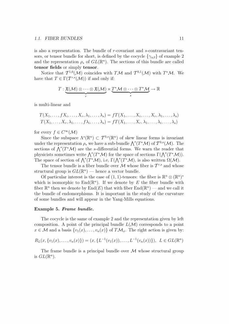
Proposition 10. Given a connection on π : P →M and a vector field X ∈X∞(M) there exists an unique vector field X ∈ X∞(P ) such that Dπ(X) =X. Moreover DRg(X) = X Rg.

Proof: The existence and uniqueness follow from TMπ(u) ≈ HuP . Thesecond claim is true by the definition of connection (see property (ii) of thedefinition).

Definition 30. We call the vector field X given by the above proposition thehorizontal lift of X.

Definition 31. Given a differentiable path γ : [0, 1] →M we say that a pathγ : [0, 1] → P is the horizontal lift of γ if π γ = γ and γ′(t) ∈ Hγ(t)P forevery t ∈ [0, 1].

Proposition 11. given a path γ : [0, 1] → M and a point u0 ∈ πγ(0) thereexists a unique horizontal lift γ of γ such that γ(0) = u0.

Proof: It follows directly from the last proposition and the existence anduniqueness of ordinary differential equations.

Definition 32. The γ given in the last proposition is called the horizontallift of γ through u0. Notice that given such an horizontal lift, it is uniquelydefined the point u1 = γ(1) ∈ π−1(γ(1)). u1 is called the parallel transportof u0 through γ

Notice that if γ lifts γ through u0 then Rg γ lifts γ through u0g. Wehave therefore a map between fibers: Υ(γ) : π−1(γ(0)) → π−1(γ(1)) suchthat Υ(γ) Rg = Rg Υ(γ).

Definition 33. Let π : P →M be a principal bundle, F a manifold in whichG acts on the left and E = (P ×F )/G the associated bundle. A connectionon E is a distribution which associates to each p ∈ E a n-dimensional vectorspace Qp such that:

(i) TEp = TFp ⊕Qp, where TFp is the tangent space to the fiber Ep ≈ Fat p.

(ii) given a differentiable path γ : [0, 1] →M and a point f0 ∈ pi−1(γ(0)there exists γ : [0, 1] → E such that γ(0) = f0 and πE γ = γ; γ defines a


isomorphism between Eγ(0) and Eγ(1) and this isomorphism depends differen-tiably on t.

(iii) p 7→ Qp is differentiable.

Theorem 4. Given a connection on π : P → M there exists a connectionon π : E →M.

Proof: ([4] p. 109) Let u and e be points in P and E respectively. Thereexists a point f in F such that uf = e. For f fixed, we have a differentiablemapping of P into E given by u ∈ P 7→ ef = e ∈ E, and it induces themap of the fiber VuP of P into the fiber Fx over x = π(u) ∈ M. Wedefine the tangent subspace Qe to be the image of VuP by this map. Since(Rg)∗(HuP ) = HugP and uaa−1f = e, this map does not depend on thechoice of u in π−1(x). It is easy to see that TEe = Fe ⊕ Ee and that thedistribution Qe is differentiable. Let γ(t), t ∈ [0, 1] be a curve in M startingat x0 and ending at x1. There exists a unique horizontal curve γ(t) in Pwhich starts at u0 and covers γ(t). Therefore γ(t)f = e(t) is an integralcurve of the distribution e 7→ Qe, which covers γ(t). Since e(t) is the mapu0f ∈ Fx0 7→ u1f ∈ Fx1 , where u1 = ˜γ(1), it gives an isomorphisms of Fx0

onto Fx1 . Hence e 7→ Qe defines a connection in E.

1.2.1 Connection on vector bundles

From now up to the end of this chapter π : E →M will be a vector bundle.Consider a principal bundle π : P → M with a connection w and an

associated vector bundle π : E → M. We want to define a differentialoperator on the sections of E. Given a local section σα : Uα → π−1(Uα) ofP define Aα = σ∗αw. Fix a vector field X ∈ X∞(M). Notice that Aα(X)is a function Aα(X) : Uα → g. The associated bundle is constructed usinga representation ρ : G → Aut(F ). Differentiating at the identity we have arepresentation of the Lie algebra ρ∗ : g → End(F ).

Define AXα : Uα → End(F ), AX

α := ρ∗ Aα(X). Given any sectionσ ∈ Γ(E) the operator ∇X : Γ(E) → Γ(E) given by

(∇Xσ)(p) = Dσ(p)(X(p)) +AXα (p)(σ(p))


is globally defined because of the compatibility conditions (see theorem 2;see also theorem 16). If we want to stress the dependence of ∇X on w or onthe corresponding family Aα we write ∇w

X , ∇AX .

Definition 34. The operator ∇X : Γ(E) → Γ(E) is called the covariantderivative with respect to X.

It is easy to check that for every a, b ∈ R (or C), every σ, τ ∈ Γ(E), everyX, Y ∈ X∞(M) and every f ∈ C∞(M) hold:(i) ∇X(aσ + bτ) = a∇Xσ + b∇Xτ .(ii) ∇aX+bY σ = a∇Xσ + b∇Y σ.(iii) ∇X(fσ) = X(f)σ + f∇Xσ (Leibniz’s rule).(iv) ∇fXσ = f∇Xσ.

Definition 35. Let E1 and E2 be vector bundles over M and L : Γ(E1) →Γ(E2) a linear map. We say that L is a differential operator of rank r iffor every f ∈ C∞(M) such that f(p) = 0, p ∈ M we have L(gr+1σ)(p) = 0for every section σ ∈ Γ(E1). The space of all differential operators of rank ris a vector space and it is denoted by Diff r(E1, E2).

From the two definitions above it follows easily that ∇X ∈ Diff 1(E,E).Notice that we have a linear map: ∇ : Γ(E) → Γ(E ⊗ T ∗M) given byσ 7→ (X 7→ ∇Xσ). Given such ∇ we can define parallel transport and hencereconstruct the connection on E. Therefore we also call ∇ connectionon E — exactly as in the principal bundle case where we use the wordconnection for both the distribution of horizontal spaces and the 1-form w.We emphasize this with a definition:

Definition 36. The linear map ∇ : Γ(E) → Γ(E ⊗ T ∗M) given by σ 7→(X 7→ ∇Xσ) is (also) called connection on E.

It easily follows:

Proposition 12. Properties:(i) ∇ ∈ Diff 1(E, E ⊗ T ∗M).(ii) ∇(fσ) = f∇σ + σ ⊗Df , where f is a function on M (Leibniz’s rule).

In general, when we have a map f : Γ(E) → Γ(E) which depends on oneor more vector fields, i.e, f = fX1,...,Xp , we can consider (as above) the mapΓ(E) → Γ(E⊗∧p(T ∗M)) given by σ 7→

((X1, . . . , Xp) 7→ fX1,...,Xp(σ)

). We

refer to this simply as “letting X1, . . . , Xp vary”.


If we have two vector bundles E1 and E2 with connections ∇1 and ∇2

we can form a connection on the sum bundle ∇1 ⊕ ∇2 : Γ(E1 ⊕ E2) →Γ((E1 ⊕ E2) ⊗ T ∗M). We also have a connection on the tensor bundle:∇1 ⊗∇2 := ∇1 ⊗ 1E2 + 1E1 ⊗∇2 : Γ(E1 ⊗ E2) → Γ((E1 ⊗ E2)⊗ T ∗M).

The following theorem give us a natural way to “transport” structuresfrom π : P →M to π : E →M.

Theorem 5. Let π : P → M be a principal bundle and π : E → M anassociated bundle with fiber F . Let C∞(P, F )G denote the space of mapsf : P → F which are equivariant to G, i.e., f(ug) = g−1f(u), u ∈ P, g ∈ G.Then there exists a one-to-one correspondence between C∞(P, F )G and Γ(E).

Proof: Let f ∈ C∞(P, F )G. Define f : P → P × F by f(u) = (u, f(u)). fis equivariant: fug = (ug, f(ug)) = (ug, g−1f(u)) = g−1(u, f(u)), where inthe last equality we used the definition of right action of G on P ×F . Take alocal section σα : Uα → P and define a section of E by sα(x) := [f(σα(x))] =[(σα(x), f(σα(x)))]. This is well defined because if σβ : Uβ → P is such thatUα ∩ Uβ 6= ∅ then σβ(x) = σα(x)gαβ(x). Hence

[f(σβ(x))] = [(σβ(x), f(σβ(x)))] = [(σα(x)gαβ(x), f(σα(x))gαβ(x))] =

[(σα(x), f(σα(x)))gαβ(x)] = [(σα(x), f(σα(x)))]

Notice that s is indeed a section since πE(s(x)) = π(σα(x)) = x and all mapsinvolved are C∞.

For the reciprocal, we remember that the associated bundle involves arepresentation ρ. We have that (recall proposition 1):

σα ∈ Γ(E) ⇔

σα : Uα → Fσβ(x) = ρ(γβα(x))σα(x)

Now we want that σα defines a function of C∞(P, F )G. But then it must bea function σα : Uα ×G → F satisfying (identifying π−1(Uα) with G× F ):

σα(x, gh) = ρ(h)−1σα(x) and σβ(x, g) = σα(x, γαβ(x)g)

Then we have σ ∈ Γ(E) 7→ σα which satisfies σα(x, g) = ρ(g)−1σα(x).Therefore

σα(x, gh) = ρ(gh)−1σα(x) = ρ(h)−1ρ(g)−1σα(x) = ρ(h)−1σα(x, g)


so:

σβ(x, g) = ρ(g)−1σβ(x) = ρ(g)−1ρ(γβα(x))σα(x) =

= ρ(g−1γβα(x))σα(x) = ρ(γαβ(x)g)−1σα(x) = σα(x, γαβ(x)g)

hence σα ∈ C∞(P, F )G.

Summarizing, the above theorem states that an equivariant function fdefines a section σf by σf (x) = [u, f(u)], u ∈ π−1(x), and a section σ de-fines an equivariant function fσ by fσ = u−1(σ(π(u))) where u is seen as anisomorphism u : F → Eπ(u) ([3] p.51).

We have an action of G on End(F ) defined by

Σ : G → Aut(End(F )), Σ(g)(L) := ρ(g)Lρ(g)−1, L ∈ End(F ), g ∈ G

Proposition 13. Let π : P →M be a principal bundle and π : E →M andassociated vector bundle with fiber F . Let w,w′ be connections on π : P →M. Then w′ − w defines a section of End(E)⊗ T ∗M.

Proof: By the last theorem is suffices to show that w′ − w defines anequivariant map P → End(F ) ⊗ (RN)∗(≈ fiber ofEnd(E) ⊗ T ∗M). LetX ∈ X∞(M). Given x ∈ M consider X(x) and p ∈ π−1(x). At p considerY ∈ TP such that Dπ(p)(Y (p)) = X(p). Define αX : P → g by αX(p) =w′(p)(Y (p))− w(p)(Y (p)) = w′(p)(YH(p) + YV (p)) + w(p)(YH(p) + YV (p)) =w′(p)(YH(p)) ∈ g, where H ,V denote the splitting with respect to w (and notw′) so that w(p)(YH(p)) = 0 but not necessarily w′(p)(YH(p)) = 0; notice alsofor every connection the action on vertical components is the same and hencew′(p)(YV (p))−w(p)(YV (p)) = 0. Now we claim that αX defines a map P → g,i.e, it does not depends on Y . Indeed, if W is another vector field such thatDπ(p)(W (p)) = X(x) then WH(p) = YH(p) (they coincide on the vertical).Now, since G acts on F through a representation ρ, differentiating at theidentity we have a map ρ∗ : g → End(F ) and hence ρ∗ αX : P → End(F ).If we let X to vary, we obtain a map ρ∗ α : P → End(F ) ⊗ (RN)∗. It iseasy to check that this map is equivariant.

Analogously:

Proposition 14. The curvature Ω on P defines a section of End(E) ⊗∧2(T ∗M).


Proof: By hypothesis there is a representation ρ : G → Aut(F ). DefineF : P → End(F )⊗∧2(RN)(≈ fiber ofEnd(E)⊗∧2(T ∗M)) by F(p)(X,Y ) :=ρ∗(Ω(p)(X, Y )), where ˜ denotes the (horizontal) lifting. Now

F(pg)(X(pg), Y (pg)) = ρ∗(Ω(pg)(X(pg), Y (pg))) = ρ∗(R∗gΩ(p)(X(p), Y (p)))

= ρ∗(Adg−1(Ω(p)(X(p), Y (p))) = Σ(g−1)(F(p)(X(p), Y (p)))

since the diagram:

gAdg−1−→ g

ρ∗ ↓ ↓ ρ∗

End(F )Σ(g−1)−→ End(F )

commutes; in the second step we used that by the definition of horizontalspace ρ∗(Ω(pg)(X(pg), Y (pg))) = ρ∗(Ω(pg)(DRg(X(p)), DRg(Y (p)))).

We have seen that w′−w defines a section of End(E)⊗T ∗M. We also haveseen that for each connection w′, w on π : P →M we have a connection onπ : E →M (see theorem 4). So it would be natural to expect that ∇w′−∇w

be a section of End(E)⊗ T ∗M. This is indeed the case:

Proposition 15. ∇w′ −∇w ∈ Γ(End(E)⊗ T ∗M).

Proof: Locally we have:

(∇w′X σ)(p) = Dσ(p)(X(p)) +AX′

α (p)(σ(p))

(∇wXσ)(p) = Dσ(p)(X(p)) +AX

α (p)(σ(p)) then:

(∇w′X −∇w

X)σ(p) = (AX′α (p)−AX

α (p))︸︷︷︸=B(p)

(σ(p))

where B is an endomorphism of the fiber (since it is the difference of twoendomorphisms).

Another way of expressing this results is to say that ∇w′X −∇w

X is an op-erator of rank zero, i.e., it depends pointwise only on the value of the sectionand not on its derivatives. The content of this proposition is already presentin the definition of the covariant derivative, since the ordinary differential is


locally a covariant derivative, so we have that the difference ∇X − D is anendomorphism. We can go one step further:

Let C(E) the space of connections on E. Given ∇0 ∈ C(E) and givena End(E)-valued 1-form A on M we define ∇A : Γ(E) → Γ(E ⊗ T ∗M) by∇Aσ = ∇0σ +A⊗ σ, where (A⊗ σ)(p)(X) = A(p)(X)(σ(p)). Then:

Corollary 2. ∇A ∈ C(E) and Γ(End(E)⊗ T ∗M) ≈ C(E)

Proof: It is a direct consequence of the last proposition.

This means that A ∈ Γ(End(E)⊗ T ∗M) defines a connection only withrespect to another one; in other words C(E) is an affine space. Bearing inmind this subtlety, physicists usually make an abuse of language and call Aitself “the connection”.

We conclude that in order to obtain a non-empty space C(E) all that wehave to prove is the existence of one connection; all the others being obtainedby adding an endomorphism.

Proposition 16. ([7]) Any principal bundle π : P →M has a connection.

Proof: As we have seen the differential is locally a connection, so that itssum with an endomorphism defines another connection. In order to definethe connection globally we take an open cover Uαα∈I over which P is trivial.For each α we have a connection wα. Let λαα∈I be a partition of unitysubordinate to the covering Uαα∈I . Define w =

∑α∈I λαwα. This is a

one-form on P with values in g. Near the pre-image of any point x ∈M thisone form is an affine combination of connections one-forms and hence is aconnection one-form. But if that is true in the neighborhood of the pre-imageof each point of M then it means that w is a connection one-form on all ofP .

Corollary 3. dim C(E) = ∞Proof: dim Γ(E) = ∞

Now let us express the curvature in terms of the connection, exactlyin the same way we did for the curvature on P . First we introduce analgebraic expression to the curvature. Then we shall express it as an exterior


covariant derivative (analogously to Ω = Dww). Finally, we shall showthat this definition coincides with that induced by Ω (the curvature on theprincipal bundle P ) — both define the same section of End(E)⊗∧2(T ∗M)(see proposition 14).

Given vector fields X,Y ∈ X∞(M) put:

F(X, Y )σ = ∇X∇Y σ −∇Y∇Xσ −∇[X,Y ]σ, σ ∈ Γ(E)

(to be honest we should use other symbol instead of F , since we are definingit and only afterwards we shall show that this definition agrees with ourprevious concept of curvature, i.e., from proposition 14; but we hope thatwith this warning there will be no misunderstanding). We write F(∇), F∇etc when we want to stress the dependence on ∇.

We notice that F is C∞(M)-linear:

F(X, fY )σ = ∇X∇fY σ −∇fY∇Xσ −∇[X,fY ]σ, f ∈ C∞(M)

= ∇X(f∇Y σ)− f∇Y∇Xσ −∇f [X,Y ]+X(f)Y σ

= f∇X∇Y σ + X(f)∇Y σ − f∇Y∇Xσ − f∇[X,Y ]σ −X(f)∇yσ

= fF(X, Y )σ

In order to prove C∞(M)-linearity in the entry F(·, Y ) we simply use theanti-symmetry F(X, Y ) = −F(Y, X) (which is obvious from the definition).

Now we show that it is C∞(M)-linear with respect to sections:

F(X,Y )(fσ) = ∇X∇Y (fσ)−∇Y∇X(fσ)−∇[X,Y ](fσ)

= ∇X(f∇Y σ + Y (f)σ)−∇Y (f∇Xσ + X(f)σ)− (f∇[X,Y ]σ + [X, Y ]σ)

= f∇X∇Y σ + X(f)∇Y σ + Y (f)∇Xσ + X(Y (f))σ − f∇Y∇Xσ−Y (f)∇Xσ −X(f)∇Y σ − Y (X(f))σ − f∇[X,Y ]σ − ([X, Y ]f)σ

= fF(X, Y )σ + X(Y (f))σ − Y (X(f))σ − ([X, Y ]f)σ = fF(X, Y )σ

What these calculations actually show is that F(X, Y ) is a section ofEnd(E) because:

Proposition 17. Let g : Γ(E) → Γ(E) be a C∞(M)-linear map. Then gdefines a section of End(E).

Remark 8. Notice that there is a straightforward reciprocal: given a sectionT ∈ End(E), T defines a map from Γ(E) to Γ(E) by σ ∈ Γ(E) by (Tσ)(x) =T (x)σ(x).


Sketch proof: Put gp = g|p, p ∈ M. We define an endomorphism of thefiber Ep, Tp : Ep → Ep by v ∈ Ep 7→ gp(σ(p)) = (gσ)(p), where σ is a sectionsuch that σ(p) = v. The definition of Tp does not depend on σ, for if σ′ is othersection such that σ′(p) = v then 0 = gp(σ(p)− σ′(p)) = gp(σ(p))− gp(σ

′(p)).To define Tp globally we use a partition of unity (more details see [8], p.220).

Now, if we let X, Y to vary we obtain that F ∈ Γ(End(E)⊗∧2(T ∗M)).Now our aim is to express F as some “derivative” of a a End(E)-valued1-form. For this we need:

Definition 37. Given a connection ∇ on a vector bundle π : E → Mwe define the exterior covariant derivative D∇ : Γ(E ⊗ ∧p(T ∗M)) →Γ(E ⊗∧p+1(T ∗M)) by

D∇µ(X1, . . . , Xp+1) :=

p+1∑j=1

(−1)j+1∇Xjµ(X1, . . . , Xj . . . , Xp+1)+

∑

1≤j<k≤p+1

(−1)j+kµ([Xj, Xk], X1, . . . , Xj, . . . , Xk, . . . , Xp+1)

Notice that D∇ naturally extends ∇, i.e., D∇ = ∇ for p = 0. Obviouslythis operator is linear. It also satisfies a Leibniz’s rule; to see this, first weapply the definition to a E-valued 1-form; it suffices to compute it for e⊗ µ:

D∇(e⊗ w)(X, Y ) = ∇X(ew(Y ))−∇Y (ew(X))− ew([X, Y ]) =

(Xw(Y ))e + w(Y )∇Xe− (Y w(X))e− w(X)∇Y e− ew([X, Y ]) =

w(Y )∇Xe− w(X)∇Y e + e(Xw(Y )− Y w(X)− w([X, Y ])

)=

(∇e ∧ w + e⊗ dw)(X, Y ) = (D∇e ∧ w + e⊗ dw)(X, Y )

where in the last step we used that D∇ = ∇ for p = 0. Proceeding induc-tively, for a E-valued p-form σ = e⊗w we get D∇(σ⊗w) = D∇e∧w+e⊗dw.

Now, if f is a differential form on M and w a form on M with values on


E, writing w = Tα ⊗ wα we obatin:

D∇(f ∧ w) = D∇(f ∧ Tα ⊗ wα) = D∇(Tα ⊗ (f ∧ wα)) =

D∇Tα ∧ f ∧ wα + Tα ⊗D∇(f ∧ wα) =

D∇Tα ∧ f ∧ wα + Tα ⊗ (df ∧ wα + (−1)deg(f)f ∧ wα) =

D∇Tα ∧ f ∧ wα + Tα ⊗ (df ∧ wα) + (−1)deg(f)Tα ⊗ (f ∧ wα) =

df ∧ (Tα ⊗ wα) + D∇Tα ∧ f ∧ wα + (−1)deg(f)Tα ⊗ (f ∧ wα)

Since D∇Tα = ∇Tα is a 1-form with values in E we have D∇Tα ∧ f =(−1)deg(f)·1f ∧D∇Tα, so we get

df ∧ (Tα ⊗ wα) + (−1)deg(f)f ∧ (D∇Tα ∧ wα + Tα ⊗ wα

)=

df ∧ w + (−1)deg(f)f ∧D∇w

which is the Leibniz rule (see [10] p. 110ff for more properties of D∇).We summarize these results:

Proposition 18. (Leibniz rule) (i) D∇(σ ⊗ w) = D∇σ ∧ w + σ ⊗ dw; (ii)D∇(f ∧ w) = df ∧ w + (−1)deg(f)f ∧D∇w.

As we said D∇ extends∇; because of that some writers also denote D∇ by∇. It is important to notice, however, that D∇ is not a connection (and thatis why we avoid to use the notation ∇). By saying that it is not a connection,we mean the following. Consider the bundle E ′ = E⊗T ∗M; it has a naturalconnection ∇′ : Γ(E ′) → Γ(E ′ ⊗ T ∗M) = Γ(E ⊗ T ∗M⊗ T ∗M) which isthe tensor connection ∇′ = ∇⊗∇L, where ∇ : Γ(E) → Γ(E ⊗ T ∗M) is theconnection on E and ∇L : Γ(T ∗M) → Γ(T ∗M⊗ T ∗M) is the connectionon T ∗M induced by the Levi-Civita connection. So we can also say that ∇′

extends ∇, as does D∇:

Γ(E)∇−→ Γ(E ⊗ T ∗M)

∇′−→ Γ(E ⊗ T ∗M⊗ T ∗M)

Γ(E)∇−→ Γ(E ⊗ T ∗M)

D∇−→ Γ(E ⊗∧

2(T ∗M))

But ∇′ is, by construction, a connection on E ′ whereas D∇ is not since itdoes not satisfy the Leibniz rule for a connection: if f is a function on Mand σ′ = σ ⊗ ω is a section of E ′ then

D∇(fσ′) = df ∧ σ′ + fD∇σ′


Which, in order to be a connection should equal df ⊗ σ′ + fD∇σ′ (see prop-erty(ii) of proposition 12)7. The reason why we are bringing attention tosuch trivial statements is that the notation used by different authors can bevery confusing: both ∇′ and D∇ are sometimes denoted by ∇ since both canbe considered extensions of the original ∇ 8. Some authors try to distinguish∇ from their extensions by denoting the extension by ∇2, but again this isnot very helpful since both ∇′ and D∇ are sometimes denoted by ∇2 (e.g.,[7] p. 85).

Theorem 6. Given a connection ∇ on π : E →M, for any section σ ∈ Γ(E)and any pair of vector fields X, Y ∈ X∞(M) we have

(D∇ ∇)(X, Y )σ = F(X, Y )σ

i.e., the curvature F is given by the composition:

F : Γ(E)∇−→ Γ(E ⊗ T ∗M)

D∇−→ Γ(E ⊗∧

2(T ∗M))

Remark 9. Now we have the following setting: the connection ∇ is identi-fied with an End(E)-valued 1-form A (corollary 2) and the curvature F iswritten as an exterior covariant derivative of such connection (actually, asthe composition D∇ ∇). So, this is the exact analogous of Ω = Dww.

Proof: Recall from definition 36 that (∇σ)(X) = ∇Xσ. Then applyingthe definition of exterior covariant derivative to the E-valued 1-form ∇σ wehave:

(D∇∇σ)(X1, X2) = ∇X1

((∇σ)(X2)

)−∇X2

((∇σ)(X1)

)− (∇σ)([X1, X2])

= ∇X1∇X2σ −∇X2∇X1σ −∇[X1,X2]σ

Now we eventually prove that the two ways of constructing the curva-ture expressed above in fact coincide. Recall from proposition 14 that thecurvature Ω on π : P → M defines a section F of End(E) ⊗∧2(T ∗M) byF(X,Y ) = ρ∗(Ω(X, Y )), where X,Y are vector fields on M, ˜ denotes theirhorizontal lift to P and ρ : G → Aut(F ) is a representation.

7D∇ does satisfy, of course, the Leibniz rule for an exterior covariant derivative.8Of course, this situation is not different from the standard situation in Riemannian

geometry, where the same symbol ∇ is used to denote the Levi-Citiva connection and itsextension to the tensor bundle.


Theorem 7. For any section τ ∈ Γ(E) we have Fτ = D∇∇τ .

Proof: We work locally. Consider a trivialization of σα : U → P . Itinduces a trivialization of E. We shall show in proposition 20 that locallyD∇∇ = dAα +Aα ∧Aα, where Aα is the End(E) valued form on U given byAα = ρ∗ σ∗αw (recall also definition of covariant derivative; the reason whydAα +Aα ∧ Aα does not have a factor 1

2as the Cartan’s structure equation

becomes clear below in the proof).We will show that the diagrams

Γ(g⊗ T ∗U)d−→ Γ(g⊗

∧2(T ∗U))

ρ∗ ↓ ↓ ρ∗

Γ(End(E)⊗ T ∗U)d−→ Γ(End(E)⊗

∧2(T ∗U))

and

Γ(g⊗ T ∗U)× Γ(g⊗ T ∗U)12∧−→ Γ(g⊗

∧2(T ∗U))

(ρ∗, ρ∗) ↓ ↓ ρ∗

Γ(End(E)⊗ T ∗U)× Γ(End(E)⊗ T ∗U)∧−→ Γ(End(E)⊗

∧2(T ∗U))

commute (again, the reason for the factor 12becomes clear in the proof). This

is a direct consequence of definitions sine d and ∧ act only on the “form part”(recall definitions 22 and 26). Explicitly, writing µ = Ti⊗µi and ν = Uj⊗νj

for g-valued forms we have that for any vector X: µ(X) = Tiµi(X); since ρ∗ is

a homomorphism ρ∗(µ(X)) = ρ∗(Tiµi(X)) = µi(X)ρ∗(Ti) = (ρ∗(Ti)⊗µi)(X),

i.e., ρ∗ (Ti ⊗ µi) = ρ∗(Ti)⊗ µi. Applying this for dµ instead of µ and usingdefinition 22: ρ∗dµ = ρ∗(Ti⊗dµi) = ρ∗(Ti)⊗dµi = d(ρ∗(Ti)⊗µi) = dρ∗µ.Analogously: ρ∗ (µ ∧ ν) = ρ∗ ([Ti, Uj] ⊗ µi ∧ νj) = ρ∗([Ti, Uj]) ⊗ µi ∧ νj.This equals [ρ∗(Ti), ρ∗(Uj)]⊗µi∧νj since ρ∗ is a (Lie algebra) representation.

Now, since d and ∧ commute with pull-backs, using Cartan’s structureequation and the previuos calculation we obtain ρ∗ (σ∗α(Ω)) = ρ∗ (σ∗α(dw+12w ∧ w)) = ρ∗ (dσ∗α(w)) + 1

2ρ∗ (σ∗α(w) ∧ σ∗α(w)) = d(ρ∗ σ∗α(w)) + 1

2ρ∗

(σ∗α(w) ∧ σ∗α(w)). The first term gives: d(ρ∗ σ∗α(w)) = dAα. For the secondterm, write σ∗αw = σ∗α(Ti ⊗ wi) = σ∗αTi ⊗ σ∗αwi. Again using the previouscalculation:

ρ∗ (σ∗α(w) ∧ σ∗α(w)) = ρ∗(σ∗αTi ⊗ σ∗αwi ∧ σ∗αTj ⊗ σ∗αwj) =

ρ∗ ([σ∗αTi, σ∗αTj]⊗ σ∗αwi ∧ σ∗αwj) = [ρ∗ σ∗αTi, ρ∗ σ∗αTj]⊗ σ∗αwi ∧ σ∗αwj


Notice that ρ∗ σ∗αTi are endomorphism of the fibers of the bundle E andwi are ordinary differential forms on U . Hence we can write σ∗αwi = f i

µdxµ,with f i

µ real valued functions on U , and denote f iµρ∗ σ∗Ti by Bµ. Then

[ρ∗ σ∗αTi, ρ∗ σ∗αTj]⊗ σ∗αwi ∧ σ∗αwj = [ρ∗ σ∗αTi, ρ∗ σ∗αTj]⊗ f iµdxµ ∧ f j

νdxν =

[f iµρ∗ σ∗αTi, f

jνρ∗ σ∗αTj]⊗ dxµ ∧ dxν = [Bµ, Bν ]⊗ dxµ ∧ dxν

Since the sum is over all µ, ν, using the anti-symmetry of [, ] and dxµ∧dxν thelast expression equals to 2BµBν ⊗ dxµ ∧ dxν , where BµBν = Bµ Bν =usualcomposition of endomorphisms. Hence

2BµBν ⊗ dxµ ∧ dxν = 2(f iµρ∗ σ∗αTi)(f

jνρ∗ σ∗αTj)⊗ dxµ ∧ dxν =

2(ρ∗ σ∗αTi)(ρ∗ σ∗αTj)⊗ f iµdxµ ∧ f j

νdxν =

2((ρ∗ σ∗αTi)(ρ∗ σ∗αTj)

)⊗ σ∗αwi ∧ σ∗αwj =

By definition of wedge product of End(E)-valued forms this last expressionequals to

2(ρ∗ σ∗αTi ⊗ σ∗αwi) ∧ (ρ∗ σ∗αTj ⊗ σ∗αwj)

Using the equality ρ∗ (Ti⊗µi) = ρ∗(Ti)⊗µi we have then ρ∗ σ∗αTi⊗σ∗αwi =ρ∗ (σ∗αTi ⊗ σ∗αwi) = ρ∗ σ∗α(T⊗wi) = ρ∗ σ∗αw. Hence

2(ρ∗ σ∗αTi ⊗ σ∗αwi) ∧ (ρ∗ σ∗αTj ⊗ σ∗αwj) = 2ρ∗ σ∗αw ∧ ρ∗ σ∗αw = 2Aα ∧ Aα

Therefore the term 12ρ∗ (σ∗α(w) ∧ σ∗α(w)) equals to Aα ∧ Aα, what finishes

the proof.

We now have the following nice picture. A connection on P induces aconnection on E, and the connection 1-form w on P (which is thought of asthe connection itself), induces a covariant derivative ∇ on E. On P exteriorcovariant derivative of w gives rise to the curvature Ω. On E exterior covari-ant derivative of ∇ gives rise to the curvature F . And this two curvatures areconnected by the representation ρ as shown in the last theorem. Moreover,we have a Cartan’s structure equation Ω = dw + 1

2w ∧ w on P and, taking

into account proposition 20 below, a structure-like equation dAα +Aα ∧Aα.Moreover, the reason why we have a factor 1

2is completely consistent with the

definition of the wedge product for g-valued and for End(E)-valued forms:


in the first case we combine the anti-symmetric wedge product of one formswith the anti-symmetric bracket of the Lie algebra what yields a symmetricterm and hence a double counting, while in the second case we just have thewedge product combined with usual multiplication of two endomorphisms(see [6] p 36).

Summarizing:

Dww = Ω = dw +1

2w ∧ w on P

D∇∇ = F = dAα +Aα ∧ Aα on E

and these quantities are related by the representation ρ.Recall that If we have two vector bundles E1 and E2 with connections ∇1

and ∇2 we can form a connection on tensor bundle. ∇1⊗∇2 : Γ(E1⊗E2) →Γ((E1 ⊗ E2) ⊗ T ∗M). In particular, since End(E) ≈ E ⊗ E∗, we have anexterior covariant derivative induced on the bundle of endomorphisms.

1.2.2 The local form of the connection and curvature

Here we investigate properties of the curvature F in local coordinates andderive some useful formulas.

This is First, we fix some notation: we shall denote (as usual) ∂µ,µ = 1, . . . , n = dim(M), a local basis of TMx; we should write ∂µ(x) forstressing that it is a basis of TMx, but we shall omit x when no confusioncan arise. Remember that locally it is always possible to write a basis ofsections for a vector bundle. We denote ei, i = 1, . . . , m = dim(F ) a localbasis of sections. Again, we should write ei(x) for Ex, but we omit the pointx when it is possible. We shall indicate indices which run from 1 to m byLatin letters and indices which run from 1 to n by Greek letters. Havingei, we can arrange a local basis of sections of E∗ as (ei)

∗ =: ei and alocal basis of sections of End(E) as ei ⊗ ej. Over all this section we shallassume that we are working in local coordinates, so that a local trivializationhas always been chosen. Therefore, for simplifying notation we shall omit theindices of local trivialization. So we shall write, for example, A instead ofAα for ρ∗ σαw appearing in the expression of the connection on E.

Recall that the connection ∇ induces a connection and an exterior co-variant derivative on the bundle End(E) — which we also denote by ∇ andD∇


We start writing the connection in local coordinates. Following physicistsnotation, we shall write ∇µ := ∇∂µ . Since ∇ associates to each pair section-tangent vector a new section we may write:

∇µej = Aiµjei

and for a general section σ = σiei and vector X = Xµ∂µ:

∇Xσ = ∇Xµ∂µ(σiei) = Xµ∇µ(σiei) =

Xµ((∂µσi)ei +Aj

µiσiej)

where in the last step we use the Leibniz rule. Renaming the dummy indicesin the last term we get:

∇Xσ = Xµ(∂µσi +Ai

µjσj)ei

If we we define the component functions ∇µσ = (∇µσ)iei the above expres-sion gives:

(∇µσ)i = ∂µσi +Ai

µjσj

which is very familiar to physicists9.

Remark 10. Physicists would write ∇µσi instead of (∇µσ)i. Definitely this

is an abuse of notation since there is no sense in taking the covariant deriva-tive of σi.

Comparing the above expression for (∇µσ)i with the expression for thecovariant derivative given in chapter 1.2:

(∇Xσ)(p) = Dσ(p)(X(p)) +AXα (p)(σ(p))

we may suspect that Aiµj are the components of the End(E)-valued form

Aα in this particular coordinate systems. This is indeed the case. First noticethat

9If σ is a section of the tangent bundle, i.e., a vector field, then Aiµj are exactly the

Christoffel symbols.


XµAiµjσ

jei = Aiµj(ei ⊗ ej ⊗ dxµ)(σ ⊗X)

Now observe that (ei ⊗ ej ⊗ dxµ) ∈ Γ(End(E|U)⊗ T ∗U), i.e., it is a localsection of the (trivial) bundle End(E|U)⊗ T ∗U over U , where U ⊂M is anopen set on which we perform the trivialization. We can also write

A(X)σ = XµAiµjσ

jei = XµAiµj(ei ⊗ ej)(σ)

Putting all pieces together we have the following expression for the co-variant derivative expressed in terms of a given local basis of sections andlocal basis of the tangent space:

(∇Xσ)i = Xσi + (A(X)σ)i = Xµ∂µσi + (A(X)σ)i

Remark 11. Physicist like to suppress the internal indices i, j which areassociated to the sections ei and write A in terms of components:

Aµ = Aiµjei ⊗ ej

In other words, by "supressing" the internal indices, we can think ofAµ as matrices representing the corresponding endomorphism in the giventrivialization; the matrix Aµ has entries Ai

µj.Now let us investigate the local form of the curvature. Define:

Fµν = F(∂µ, ∂ν)

Fµν is a section of End(E). Notice that since [∂µ, ∂ν ] = 0 we also haveFµν = [∇µ,∇ν ]. The linearity properties of the curvature allow us to writefor any pair of tangent vectors X = Xµ∂µ and Y = Y ν∂ν :

F(X,Y ) = XµY νFµν

Now we compute:


Fµνei = ∇µ∇νei −∇ν∇νe−∇[∂µ,∂ν ]ei

∇µ(Ajνiej)−∇ν(Aj

µiej) =

(∂µAjνi)ej +Ak

µjAjνiek − (∂νAj

µi)ej −AkνjAj

νiek =((∂µAj

νi)− (∂νAjµi) +Aj

µkAkνi −Aj

νkAkνi

)ej (∗)

where we used [∂µ, ∂ν ] = 0 and in the last step we simply relabeled theindices. Analogously to what we did for the connection we may expand thecurvature in a local basis ei ⊗ ej of End(E):

Fµν = F jµνiej ⊗ ei

the functions F jµνi are called components of the curvature (in that local basis).

Notice:

Fµνei = F jµνiej

So, comparing with (∗) we have:

F jµνi = (∂µAj

νi)− (∂νAjµi) +Aj

µkAkνi −Aj

νkAkνi

Again, physicists like to suppress the internal indices i, j, k associated tothe basis of sections of E over U , meaning that Aµ is thought of as a matrixand then we may write the above expression as:

Fµν = ∂µAν − ∂νAµ + [Aµ, Aν ]

Now that we expressed the functions Fµν in a local basis ei ⊗ ej ofEnd(E) we can write the curvature itself in terms of the “components” Fµν :

F =1

2Fµνdxµ ∧ dxν

the factor 12appears because we are summing over all indices and not

only over µ < ν.Now we show that D∇ ∇ is proportional to the curvature.


Lemma 2. For any section α of E we have

∇α = ∇µα⊗ dxµ

Proof: For any vector field X:

(∇α)(X) = ∇Xα = Xµ∇µα = (∇µα⊗ dxµ)(X)

Lemma 3. For any E-valued p-form α, written locally as α = αiei⊗wIdxI =αieiwI ⊗ dxI := αI ⊗ dxI with dxI = dxµ1 ∧ · · · ∧ dxµp, we have:

D∇α = ∇ναI ⊗ dxν ∧ dxI

Proof: Compute:

D∇α = D∇(αI ⊗ dxI) = (∇αI) ∧ dxI + αI ⊗ ddxI = (∇αI) ∧ dxI

= ∇ναI ⊗ dxν ∧ dxI

Proposition 19. For any E-valued p-form α we have:

D∇ D∇α = F ∧ α

Proof: As before, write α = αI ⊗ dxI , where dxI = dxi1 ∧ · · · ∧ dxip .

D∇D∇α = D∇(∇ναI ⊗ dxν ∧ dxI)

= ∇τ∇ναI ⊗ dxτ ∧ dxν ∧ dxI

=1

2[∇τ ,∇ν ](αI)⊗ dxτ ∧ dxν ∧ dxI

=1

2Fτν(αI)⊗ dxτ ∧ dxν ∧ dxI = F ∧ α

It is a easy calculation to show that if µ is and End(E)-valued p-form andσ is a E-valued form we have D∇(µ ∧ σ) = (D∇µ) ∧ σ + (−1)pµ ∧D∇σ.


Theorem 8. (Bianchi Identity) D∇F = 0.

Proof: For any E-valued form we α have

(D∇)3 = D∇(D∇D∇α) = D∇(F ∧ α) = (D∇F) ∧ α + F ∧ (D∇α)

On the other hand:

(D∇)3α = (D∇)2(D∇α) = F ∧D∇α

So D∇F = 0.

Remark 12. Although the Bianchi has been deduced used some computationscarried out on local coordinates — namely, proposition 19 — it is easy tosee that it holds globally. Indeed, it states that D∇F = 0 at leat locally.But the null section is defined globally and and equals D∇F on every localtrivialization. So we should have D∇F = 0 globally. We claim — withoutproving, however — that proposition 19 itself holds globally. These remarkswill be useful on section 4.3.2.

Lemma 4. For any E-valued form α we have D∇α = dα +A ∧ α

Proof: Using lemma 3 and recalling A = Aiµjei ⊗ ej ⊗ dxµ = Aµ ⊗ dxµ

D∇α = ∇µαI ⊗ dxµ ∧ dxI = (∂µ +Aµ)αI ⊗ dxµ ∧ dxI =

∂µαI ⊗ dxµ ∧ dxI +Aµ(αI)⊗ dxµ ∧ dxI =

dα +A ∧ α

Notice that we are using that locally the usual derivative is a covariant deriva-tive.

Proposition 20. F = dA+A ∧A.Proof: For any E-valued form α:

D∇D∇α = D∇(dα +A ∧ α) = d(dα +A ∧ α) +A ∧ (dα +A ∧ α) =

d(A ∧ α) +A ∧ dα +A ∧A ∧ α =

dA ∧ α−A ∧ dα +A ∧ dα +A ∧A ∧ α =

= (dA+A ∧A) ∧ α

On the other hand D∇D∇α = F ∧ α. The result follows.


Remark 13. This is only another way of writing:

Fµν = ∂µAν − ∂νAµ + [Aµ, Aν ]

Chapter 2

Clifford Algebras

Let V be a finite dimensional vector space over R with a quadratic form<,>. Denote by ‖ x ‖= √

< x, x > We are using the notation of innerproduct because in most applications we have so, but <, > needs to be onlya quadratic form. Consider the tensorial algebra

T (V ) =⊕n≥0

V ⊗ V ⊗ · · · ⊗ V︸︷︷︸n times

=

R⊕ V ⊕ V ⊗ V ⊕ · · ·Denote by I(V ) the two-sided ideal generated by v⊗w+w⊗v+2 < v,w > ·1.Definition 38. In the above notation the Clifford algebra of V is Cl(V ) :=T (V )/I(V ).

In other words, Cl(V ) is an associative R-algebra with unity generatedby V subjected to the relations v ⊗ w + w ⊗ v = −2 < v, w > ·1. We shallusually write vw instead of v⊗w and < v, w > instead of < v, w > ·1. Noticethat if e1, . . . , en is an orthonormal basis of V we have ejek = −ekej forj 6= k. It also follows from the definition that v2 = − ‖ v ‖2.

Lemma 5. (Fundamental lemma of Clifford algebras). Let φ : V → Aa linear map, where A is an associative algebra with unity. If it happensφ(v) · φ(v) = − ‖ v ‖2 f for every v ∈ V then φ has a unique extension foran homomorphism of algebras (also denoted by φ) φ : Cl(V ) → A.

Proof: The fundamental theorem for tensorial algebras guarantees that φuniquely extends to T (V ) as an homomorphism of algebras. The condition

47

48 CHAPTER 2. CLIFFORD ALGEBRAS

φ(v) · φ(v) = (φ(v))2 = − ‖ v ‖2 imply that ker(φ : T (V ) → A) containsI(V ) and hence φ descends to the quotient.

Remark 14. If dim(V ) = n we usually write Cl(V ) = Cl(n).

Notation: From now up to the end of this chapter e1, . . . , en willdenote an orthonormal basis of V .

Notice that any ξ ∈ Cl(V ) is uniquely written as

ξ = a0 +n∑

k=1

∑j1<···<jk

aj1,...,jkej1 · · · ejk

where aj1,...,jk∈ R. If follows that Cl(V ) is a vector space of dimension 2n

(notice that Cl(V ) is isomorphic, as vector space, to∧∗ V ). If we denote

by Cl0(V ) (Cl1(V )) the subspaces of Cl(V ) containing only an even (odd)number of elements on the base we have a Z2-graded splitting Cl(V ) =Cl0(V )⊕Cl1(V ) . Notice that Cl0(V ) is a sub-algebra and Cl1(V ) is a moduleover Cl0(V ). The elements of Cl0(V ) (Cl1(V )) commute (anti-commute)among themselves1.

Proposition 21. If (V1, <,>1) and (V2, <, >2) are vector spaces endowedwith quadratic forms which are preserved by a linear map f : V1 → V2 thenf uniquely extends to f : Cl(V1) → Cl(V2).

Proof:

f(x)f(x) = − < f(x), f(x) >2=< x, x >1= − ‖ x ‖2

The results follows from the fundamental lemma.

Remark 15. If (V3, <, >3) is other vector space with a quadratic form pre-served by g : V2 → V3, then gf : V1 → V3 uniquely extends to a map betweenthe algebras. By uniqueness this must be the composition of the extensionsof f and g.

Denote by Aut(Cl(V )) the automorphisms of Cl(V ) which preserve V .1Z2-graded algebras such that the splitting if given in terms of commuting and anti-

commuting parts are called in physicists’ literature superalgebras

2.1. THE ISOMORPHISM AUT(CL(V )) ≈ O(V ) 49

Proposition 22. Aut(Cl(V )) ≈ O(V ).

Proof: f ∈ O(V ) uniquely extends to an automorphism of Cl(V ) (use thefundamental lemma and the above remark applied to g = f−1). Reciprocally,if f ∈ Aut(Cl(V )) then

< f(v), f(v) >= −f(v)f(v) = f(−v2) = f(‖ v ‖2) =‖ v ‖2 f(1) =< v, v >

In the next section we shall give an explicit description of the action ofO(V ) on Cl(V ). Such description will be useful when we consider spinorbundles.

2.1 The isomorphism Aut(Cl(V )) ≈ O(V )

Since Cl(V ) is an algebra with unity we can consider the group of units ofCl(V ) (i.e., the group of elements of Cl(V ) which are invertible), denoted byClx(V ). Notice that if < v, v > 6= 0 then v ∈ Clx(V ); indeed v−1 = − v

‖v‖2 .Clx(V ) is a Lie group of dimension 2n whose Lie algebra Cl(V ) is Cl(V )

itself. We have the adjoint representation ad : Clx(V ) → Aut(Cl(V )),adu(x) = uxu−1 (a simple calculation shows that ad is indeed a representa-tion). Derivating at the identity:

d

dt(adexp(tY )(X))|t=0 = Y X −XY = [Y,X]

so we have a representation of the Lie algebra: Ad : Cl(V ) → End(Cl(V )),Y 7→ [Y, ·]. Since

[Y, X]Z + X[Y, Z] = [Y, XZ]

we have that [Y, ·] is actually a derivation of the Lie algebra, so we haveAd : Cl(V ) → Der(Cl(V )).

Proposition 23. Let v, w ∈ V , < v, v > 6= 0 and v⊥ the space orthogonal tov. Then −adv(w) = −vwv−1 = w − 2<v,w>

<v,v>v = Rv⊥(w), where Rv⊥ denotes

the reflexion through v⊥.


Proof: Since v−1 = −v/ < v, v > we have (using vw +wv = −2 < v, w >):

− < v, v > adv(w) = − < v, v > vwv−1 = vwv

= −v2w − 2 < v,w > v =< v, v > w − 2 < v, m > v

Corollary 4. ad ∈ Aut(Cl(V )).

Proof: From the above proportion we have adv(V ) = V .

Up to a minus signal, we have that adv is a reflection through v⊥. Inorder to get a reflection we consider:

Definition 39. The twisted adjoint representation ad : Clx(V ) → Aut(Cl(V ))is given by adu(x) = α(u)xu−1, where α : Cl(V ) → Cl(V ) is the automor-phism which extends α : V → V , α(v) = −v (the existence of such extensionis guaranteed by the fundamental lemma).

A straightforward calculation gives:

Proposition 24. adv(w) = w − 2<v,w><v,v>

v = Rv⊥(w)

Denote by P (V ) the subgroup of Clx(V ) whose elements are such thatad(V ) = V . Restricting ad we get a representation ad : P (V ) → Aut(CL(V ).

Proposition 25. The kernel of ad : tildeP (V ) → Aut(CL(V ) is the set ofnon-null multiples of 1 (i.e. R or occasionally C).

Proof: [11] p. 14

Proposition 26. adu : V → V preserves <,> for every u ∈ P (V ). So wehave a homomorphism ad : P (V ) → O(V )

Proof: [11] p. 16

2.1. THE ISOMORPHISM AUT(CL(V )) ≈ O(V ) 51

Consider now the subgroup P (V ) of P (V ) generated by elements v ∈ Vsuch that < v, v > 6= 0, i.e.,

P (V ) = v1 · · · vr ∈ Cl(V ) :< vi, vi >6= 0, v1, . . . , vr is a finite sequence of V Restricting ad to P (V ) ⊂ P (V ) we get a homomorphism ad : P (V ) →

O(V ). Since for each v ∈ V adv = Rv⊥ and every element of P (V ) is aproduct of vectors v ∈ V , we get:

adv1···vr = Rv⊥1 · · · Rv⊥r

By the Cartan-Dieudonné theorem O(V ) is generated by reflections, so ad :P (V ) → O(V ) is onto. On the other hand, restricting ad : P (V ) →Aut(Cl(V )) to P (V ) we get another homomorphism ad : P (V ) → Aut(Cl(V )).We have therefore two homomorphisms:

Aut(CL(V ))

ad : P (V ) O(V )

But by 22 we have:

Aut(CL(V ))

ad : P (V ) ↓≈ O(V )

As the non-null multiples of 1 belong to P (V ), proposition 25 gives, to-gether with the surjectivity of ad : P (V ) → O(V ) that:

Theorem 9. ad : P (V )/ kerad : P (V ) → O(V ) ≈ O(V ) ≈ Aut(CL(V )

This is the main result of this section. It means that the action of O(V )

on CL(V ) is adjoint-like, i.e., any automorphism of Aut(CL(V )) is writtenas

adv1···vr = adv1 · · · advr

where v1, . . . , vr ∈ P (V ).The Cartan-Dieudonné theorem also tells us that each element of SO(V )

is written as an even number of reflections. Considering SP (V ) := P (V ) ∩Cl0(V ) and proceeding in analogous fashion we get


Theorem 10. ad : SP (V )/ kerad : SP (V ) → SO(V ) ≈ SO(V ) ⊂Aut(CL(V )

This means that SO(V ) acts on Cl(V ) by

adv1···v2r = adv1 · · · adv2r

2.2 The groups Pin and Spin

Definition 40. Pin(V ) is the subgroup of Clx(V ) generated by elementsv ∈ V such that ‖ v ‖2= 1. In other words:

Pin(V ) := ξ ∈ Clx(V ) : ξ = u1 · · ·uk, uj ∈ V, ‖ uj ‖= 1

We also define: Spin(V ) := Pin(V ) ∩ Cl0(V ), in other words:

Spin(V ) := ξ ∈ Clx(V ) : ξ = u1 · · · u2k, uj ∈ V, ‖ uj ‖= 1

Some important remarks: (i) There exists an obvious homomorphismCl(V ) → Z2, Cl0(V ) 7→ 1, Cl1(V ) 7→ −1. If we restrict to Pin(V ) thenSpin(V ) is the kernel of Pin(V ) → Z2. (ii) If ξ = u1 · · ·uk ∈ Pin(V ) thenξ−1 = (−uk) · · · (−u1) ∈ Pin(V ) (since v−1 = − v

‖v‖2 for < v, v > 6= 0).The group Spin(V ) acts on Cl(V ) by Spin(V )×Cl(V ) → Cl(V ), (σ, ξ) 7→

adσ = σξσ−1. Notice that here is not necessary to consider the twisted ad-joint representation because the elements of Spin(V ) are products of aneven number of vectors v ∈ V — so that the cumbersome minus signdisappears. By the results of the last section adσ preserves V for everyσ ∈ Spin(V ), hence we have a representation of Spin(V ) on Cl(V ), i.e.,ad : Spin(V ) → Aut(Cl(V )), σ 7→ adσ.

Some of the next results could be derived directly from theorem 10, butwe shall provide explicit calculations.

Lemma 6. The image of the representation of Spin(V ) on Cl(V ) consistsof automorphisms which preserve V and orientation. Therefore we have amap from Spin(V ) onto SO(V ).

Proof: We have already seen that adσ preserves V . Notice that for eachw ∈ V with ‖ v ‖= 1, we have that adw(v) = −Rx⊥(v). Then, for ξ =u1 · · · u2k ∈ Spin(V ), adξ is an even composition of reflections and hence it

2.2. THE GROUPS PIN AND SPIN 53

preserves orientation. Since each element of SO(V ) is written as an evennumber of reflections, we have the result.

Lemma 7. The kernel of the representation ad : Spin(V ) → Aut(Cl(V )) isSpin(V )∩cen(Cl(V )), where cen(Cl(V )) is the center of the Clifford algebra.

Proof: obvious.

From the surjectivity of Spin(V ) onto SO(V ) we get an isomorphismSpin(V )/(Spin(V )∩cen(Cl(V )) ≈ SO(V ). So it is important to understandcen(Cl(V )).

Lemma 8. If dim(V ) is even then cen(Cl(V )) = R; if dim(V ) is odd thancen(Cl(V )) = span1, e1 · · · en ≈ R⊕ R.

Proof: Fix an orthonormal basis e1, . . . , en and notice that ej·(ej1 · · · ejt) =±(ej1 · · · ejt) · ej, where the sign is (−1)t if j 6= jr for every 1 ≤ j ≤ t and(−1)t−1 if j = jr for some r ∈ 1, . . . , t. The result follows by inspection.

Lemma 9. Spin(V ) ∩ cen(Cl(V )) = +1,−1.

Proof: From the definition of Spin(V ) it follows that Spin(V )∩cen(Cl(V )) =Spin(V )∩cen(Cl0(V )) = Spin(V )∩R. Spin(V ) is generated by unitary vec-tors v and the multiplication of two such vectors can result only in either +1or −1 (v2 = −1, v(−v) = 1). Then Spin(V ) ∩ R = +1,−1.

Putting these lemmas together:

Theorem 11. Spin(V )/+1,−1 ≈ SO(V ).

The important fact here is that Spin(V ) is not a double copy of SO(V ):

Theorem 12. If dim(V ) ≥ 2 then Spin(V ) → SO(V ) is a non-trivial doublecover.


Sketch proof: Let W be a 2-dimensional subspace of V . Notice that thepre-image of SO(W ) ⊂ SO(V ) is Spin(W ) ⊂ Spin(V ). It suffices to showthat Spin(W ) → SO(W ) is a non-trivial double cover (since π1(SO(W )) →π1(SO(V )) is surjective). Now notice that Cl(W ) ≈ H, Spin(W ) ≈ S1 ⊂ Cand W ≈ Spanj,k. Therefore the conjugation of Spin(W ) on W is simplythe square of the usual action of S1 on W .

It follows from the above theorem that if dim(V ) = n then Spin(V ) is acompact Lie group of dimension n(n− 1)/2, which is connected if n > 1 andsimply connected if n > 2 — so for n > 2 the group Spin(V ) is a universalcover of SO(V ) and then the Lie algebras spin(V ) of Spin(V ) and so(V ) ofSO(V ) are isomorphic.

2.3 Classification of Clifford algebrasLet Cl(V ) be the complexification of Cl(V ), i.e., Cl(V ) = Cl(V ) ⊗ C. Thisis equivalent of considering complex coefficients on the linear combinations.Given an orthonormal basis e1, . . . , en define:

wC := i[n+1

2]e1 · · · en

where i is the imaginary number and [·] is the integer part. A simply calcu-lation shows that wC is independent of the choice of basis and that w2

C = 1.wC acts on Cl(V ) by left multiplication. From w2

C = 1 it follows that wecan decompose Cl(V ) in Cl+(V ) and Cl−(V ), eigenspaces associated to ±1eigenvalues (v ∈ Cl±(V ) if and only if wCv = ±v).

Notice that if dim(V ) is even, then wC ∈ cen(Cl0(V )) and wC anti-commutes with Cl1(V ). If dim(V ) is odd, then wC ∈ cen(Cl(V )).

Proposition 27. If dim(V ) is odd then the splitting Cl+(V ) ⊕ Cl−(V ) isorthogonal (i.e.: Cl±(V ) are subalgebras which annihilates each other) andCl±(V ) are both isomorphic to Cl0(V ) (isomorphism of algebras).

Proof: Take u ∈ Cl+(V ) and v ∈ Cl−(V ). Then wCu = u and wCv = −v.Since wC is on the center of Cl(V ) (because the dimension of V is odd) wehave wCuwCv = u(−v) = w2

Cuv = uv, so uv = −uv and therefore uv = 0.For the isomorphism, notice that wC alternates Cl0(V ) and Cl1(V ), hence

Cl0(V ) ∩ Cl±(V ) = 0. It follows that the compositions:

Cl0(V ) → Cl(V )π±−→ Cl±(V )

2.3. CLASSIFICATION OF CLIFFORD ALGEBRAS 55

are algebra isomorphisms.

Remark 16. notice that this embedding of Cl0(V ) is the graph o f an iso-morphism Cl+(V ) ≈ Cl−(V ).

We have an analogous result for the case of even dimension:

Proposition 28. If dim(V ) is even then there is an orthogonal splittingCl0(V ) = Cl+0 (V )⊕ Cl−0 (V ) and there is an algebra isomorphism Cl+0 (V ) ≈Cl−0 (V ). Moreover, Cl+0 (V ) is isomorphic (as algebra) to Cl(W ), where W ⊂V is a codimension 2 subspace.

Proof: The orthogonal splitting follows, analogously to the above proposi-tion, from the fact that for each n even we have wC ∈ cen(Cl0(V )). Noticethat there is an isomorphism Cl0(V ) ≈ Cl(W ′), where W ′ is a subspace ofcodimension 1. Indeed dim(Cl0(V )) = 2n/2 = 2n−1 = dim(Cl(W ′)), givena vector space isomorphism. Since dim(W ′)=odd, by the above proposi-tion we have Cl(W ′) = Cl+(W ′)⊕ Cl−(W ′), hence we have the algebra iso-morphism Cl+0 (V ) ≈ Cl+(W ′). Using again the above proposition we haveCl+(W ′) ≈ Cl0(W

′), so Cl+0 (V ) ≈ Cl0(W′) (algebra isomorphism). Take

now W ⊂ W ′ a subspace of codimension 1. We have an algebra isomorphismCl0(W

′) ≈ Cl(W ). The result follows.

Proposition 29. Similar result hold for Cl1(V ), i.e., Cl1(V ) = Cl+1 (V ) ⊕Cl−1 (V ).

Proof: Analogous.

Summarizing, if the dimension of V is:

even:wC ∈ cen(Cl0(V )), Cl0(V ) ≈ Cl+0 (V )⊕ Cl−0 (V ), Cl1(V ) ≈ Cl+1 (V )⊕ Cl−1 (V ),Cl+0 (V ) ≈ Cl0(W ) ≈ Cl−0 (V )

odd:wC ∈ cen(Cl(V )), Cl(V ) ≈ Cl+(V )⊕ Cl−(V ),Cl0(V ) ≈ Cl+(W ) ≈ Cl−(V )


The lemma 11 below is the key lemma to classify Clifford algebras. Inorder to prove this lemma we must understand the tensor product of Cliffordalgebras.

We start recalling that if A and B are algebras with unit over K thenthe tensor product A⊗B is the algebra whose the underlying vector space isthe tensor product of A and B and whose multiplication on simple elementsis given by

(a⊗ b) · (a′ ⊗ b′) = (aa′)⊗ (bb′)

If, however A = A0 ⊕ A1 and B = B0 ⊕B1 are Z2-graded algebras then wecan introduce a second Z2-graded multiplication by the rule

(a⊗ b) · (a′ ⊗ b′) = (−1)deg(b) deg(a′)(aa′)⊗ (bb′)

for pure degree elements. The resulting algebra is called Z2-graded tensorproduct and is denoted by ⊗. It is also Z2-graded:

(A⊗B)0 = A0 ⊗B0 + A1 ⊗B1

(A⊗B)1 = A1 ⊗B0 + A0 ⊗B1

Lemma 10. Let V = V1⊕V2 be a <,>-orthogonal decomposition of V (i.e.,< v1 + v2, v1 + v2 >=< v1, v1 > + < v2, v2 > for v1 ∈ V1 and v2 ∈ V2). Thenthere exists an isomorphism of Clifford algebras:

Cl(V ) ≈ Cl(V1)⊗Cl(V2)

where the quadratic form on Vi is <,> restricted to Vi.

Proof: Consider the map f : V → Cl(V1)⊗Cl(V2) given by f(v) = v1 ⊗1 + 1 ⊗ v2 where v = v1 + v2 is the decomposition of v with respect to thesplitting V = v1 ⊕ V2. From the <,>-orthogonality and the definition ofZ2-graded tensor product we have that

f(v) · f(v) = (v1 ⊗ 1 + 1⊗ v2)2 = v2

1 ⊗ 1 + 1⊗ v22 =

− < v1 + v2, v1 + v2 > 1⊗ 1 = − < v, v > 1⊗ 1

Hence by the fundamental lemma f extends to an algebra homomorphismf : Cl(V ) ≈ Cl(V1)⊗Cl(V2). The image of f is a subalgebra which containsCl(V1) ⊗ 1 and 1 ⊗ Cl(V2). Therefore f is onto. The injectivity followseasily by considering a basis for Cl(V ) generated by a basis of V which iscompatible with the splitting.


Lemma 11. Cl(V ⊕ R2) ≈ Cl(V )⊗ Cl(R2)

Proof: Let v1, . . . , vn be an orthonormal basis of V and e1, e2 anorthonormal basis of R2. Define: φ : V ⊕ R2 → Cl(V ) ⊗ Cl(R2) by vj 7→ivj⊕ e1e2, 1 ≤ j ≤ n and ej 7→ 1⊗ ej, j = 1, 2. We shall show that for everyui, uj belonging to the basis of V ⊕ R2 we have (φ(ui))

2 = − ‖ ui ‖2 andφ(ui)φ(uj) + φ(uj)φ(ui) = 0 if i 6= j. A straightforward calculation showsthat this is equivalent to the fundamental lemma and so it gives an extensionφ : Cl(V ⊕ R2) → Cl(V )⊗ Cl(R2).

Compute:

φ(vj)φ(vj) = (ivj ⊗ e1e2)(ivj ⊗ e1e2) = −vjvj ⊗ e1e2e1e2 =

= vjvj ⊗ e2e1e1e2 = v2j ⊗ 1 = − ‖ vj ‖2

The remaining calculations are analogous. So we have the desired extension.Notice that since φ takes the generators of Cl(V ⊕ R2) onto the generatorsof the Cl(V )⊗Cl(R2) we have an isomorphic of algebras since both have thesame dimension.

Now we notice that Cl(R) ≈ C, what implies Cl(R) ≈ C ⊕ C; andCl(R2) ≈ H, what implies Cl(R2) ≈ H ⊕ C. Define a map H → MC(2) (=complex 2× 2 matrices) by

α + jβ 7→(

α −β∗

β α∗

)

α, β ∈ C, we have an algebra isomorphism H ⊗ C ≈ MC(2). We obtaintherefore the followingInductive rule: using the lemma 11 and H ⊗ C ≈ MC(2) we can getinductively all the complex Clifford algebras.

Theorem 13. If dim(V ) = 2m than Cl(V ) ≈ MC(2m); if dim(V ) = 2m + 1

than Cl(V ) ≈ MC(2m)⊕MC(2

m).

Proof: Use the inductive rule and the isomorphic MC(m) ⊗ MC(k) ≈MC(mk).

Corollary 5. If dim(V ) = 2m then Cl+0 (V ) ≈ MC(2m−1).


Proof: Use theorem 13 and proposition 28.

We recall some definitions:

Definition 41. If A is an algebra with unity and V is a finite dimensionalvector space than a linear map ρ : A → End(V ) such that ρ(ab) = ρ(a)ρ(b)and 1 7→ id is called a representation of A on V . The dimension ofthe representation is the dimension of V . Two representations ρ1 : A →End(V1) and ρ2 : A → End(V2) are said to be equivalent if there exists alinear and invertible map f : V1 → V2 such that ρ2(a) = f ρ1(a) f−1 forevery a ∈ A.

If ρ1 : A → End(V1) and ρ2 : A → End(V2) are two representations of Ait follows that ρ = ρ1⊕ρ2 : A → End(V1⊕V2), given by ρ(a) = ρ1(a)⊕ρ2(a)is also a representation.

Definition 42. A representation ρ which can be written as ρ = ρ1 ⊕ ρ2 iscalled reducible; otherwise it is called irreducible.

Theorem 14. If dim(V ) = 2m then Cl(V ) has an unique (up to isomor-phism) irreducible representation of dimension 2m.

Proof: By theorem 13 we have an isomorphism Cl(V ) ≈ MC(2m). By the

Werderburn theorem End(C2m) has an unique (up to isomorphism) represen-

tation of dimension 2m and in fact End(C2m) ≈ MC(2

m).

Notice that the action of Cl(V ) on C2m induces a isomorphism Cl(V ) ≈End(C2m

) ≈ C2m ⊗ (C2m)∗.

Theorem 15. If dim(V ) = 2m+1 then Cl(V ) has two irreducible representa-tion (up to isomorphism) of dimension 2m. Moreover: Cl0(V ) ≈ End(C2m

).

Proof: We have the isomorphisms:

Cl(V ) ≈ Cl+(V )⊕ Cl−(V )prop.27≈ Cl0(V )⊕ Cl0(V )

Using theorem 13 on the other hand

Cl(V ) ≈ MC(2m)⊕MC(2

m)Wederburn≈ End(C2m

)⊕ End(C2m

)


Definition 43. The action of Cl(V ) on C2m and C2m⊕C2m through the aboveisomorphisms is called Clifford multiplication. It is sometimes denoted bya dot: “·”.

Let dim(V ) = 2m and consider the irreducible representation of Cl(V )on C2m . Through this representation wC becomes a map wC : C2m → C2m

and therefore we have C2m= (C2m

)+ ⊕ (C2m)−. We use this to prove:

Theorem 16. Let dim(V ) = 2m and consider the irreducible representa-tion of Cl(V ) on C2m. Clifford multiplication induces the following isomor-phismm:

Cl+0 (V ) ≈ End((C2m)+)

Cl−0 (V ) ≈ End((C2m)−)

Cl+1 (V ) ≈ Hom((C2m)−, (C2m)+)

Cl−1 (V ) ≈ Hom((C2m)+, (C2m)−)

Proof: We recall that if dim(V )=even then wC commutes with Cl0(V ) andanti-commutes with Cl1(V ). Denote by ˆ the images of elements in Cl(V ) bythe isomorphism End(C2m

).If u ∈ Cl+0 (V ) then wCu = uwC (because it belongs to Cl0(V )) and

wCu = u (because it belongs to Cl+(V )). Take h ∈ (C2m)+. We have:

u wC(h) = u(h) = wC(u(h))

what means that u(h) is an eigenvector of wC with eigenvalue +1 and there-fore u(h) ∈ (C2m

)+, i.e., u leaves (C2m)+ invariant. On the other hand, if

h ∈ (C2m)− then:

u wC(h) = −u(h) = u(h)

since wCu = u. Therefore u(h) = 0 and hence u ∈ End((C2m)+). The

isomorphism Cl−0 (V ) ≈ End((C2m)−) is proven in analogous fashion.

Take now v ∈ Cl+1 (V ). Then wCv = −vwC and wCv = v. If h ∈ (C2m)−

we havewC(v(h)) = −v(−h) = v(h)

what implies v(h) ∈ (C2m)+. Now for h ∈ (C2m

)− we have

wC v(h) = v(h)


andwC v(h) = −v wC(h) = −v(h)

what implies v(h) = 0 and therefore h ∈ Hom((C2m)−, (C2m

)+). The proofis analogous for Cl−1 (V ).

Remark 17. For dim(V ) = 2, considering the isomorphism Cl(V ) ≈ End(C2m)

we can give a nice interpretation to the last theorem. The splitting Cl(V ) =Cl+0 (V )⊕Cl−0 ⊕Cl+1 (V )⊕Cl−1 (V ) implies that if we write a vector v ∈ C2m

=(C2m

)+⊕ (C2m)− as v = v+ + v−, then a matrix M ∈ MC(2

m) can be writtenas:

M =

(A 00 0

)

︸︷︷︸(C2m)+→(C2m)+

+

(0 00 B

)

︸︷︷︸(C2m)−→(C2m)−

+

(0 C0 0

)

︸︷︷︸(C2m)−→(C2m)+

+

(0 0D 0

)

︸︷︷︸(C2m)+→(C2m)−

where A,B,C,D ∈ MC(2m−1).

Since Spin(V ) ⊂ Cl(V ) we can restrict the representations of Cl(V ) andsuch a way we obtain:

Proposition 30. There exists an unique (complex) representation of Spin(V ),∆C : Spin(V ) → Aut(C2m

), which is induced by irreducible representationsof Cl(V ).

Proof: It follows from Spin(V ) ⊂ Cl0(V ) and theorem 14.

Proposition 31. If dim(V ) = 2m then ∆C splits in two inequivalent repre-sentations, ∆C = ∆+

C⊕∆−C , each one of dimension 2m−1. If dim(V ) = 2m+1

then ∆C is a 2m-dimensional irreducible representation of Spin(V ).

Sketch proof: For dim(V ) = 2m we have Cl0(V ) = Cl+0 (V ) ⊕ Cl−0 (V ),Cl+0 (V ) ≈ End((C2m

)+) and Cl−0 (V ) ≈ End((C2m)−). So, restricting to

Spin(V ) ⊂ Cl0(V ) these isomorphisms give ∆+C : Spin(V ) → Aut((C2m

)+)and ∆+

C : Spin(V ) → Aut((C2m)+). It follows from theorem 16 that these

are the only irreducible inequivalent representations (up to isomorphism) ofSpin(V ). We also have dim((C2m

)+) = dim((C2m)−) = 2m/2 = 2m−1.

2.4. THE GROUP SPINC 61

For dim(V ) = 2m + 1 theorem 15 give us two 2m-dimensional irreduciblerepresentations of Cl(V ) and Cl0(V ) ≈ End(C2m

). The result follows fromSpin(V ) ⊂ Cl0(V ).

A detailed proof can be found in [12] p. 19.

Remark 18. We are not saying — and it is not true — that ∆C is theunique complex irreducible representation of Spin(V ) for dim(V ) = 2m + 1neither that ∆±

C are the only two irreducible representations of Spin(V ) fordim(V ) = 2m. What we claim is that these are the only ones which extendto (automatically irreducible) representations of Cl0(V ).

2.4 The group Spinc

Definition 44. The subgroup of Clx(V ) generated by Spin(V ) and S1 iscalled the Spinc(V ) group, i.e.,

Spinc(V ) := a ∈ Clx(V ) : a = a0u1 · · ·u2k, a0 ∈ S1, ui ∈ V, ‖ ui ‖= 1

Proposition 32. Spinc(V ) ≈ Spin(V )× S1/(1, 1), (−1,−1).Proof: Define a map Spin(V ) × S1 → Spinc(V ) by (σ, a) 7→ aσ. Sinceelements of S1 commute with elements of Spin(V ) such map is onto. Itskernel are elements of the form (σ, σ−1) because aσ = 1 gives a = σ−1. Itfollows from lemmas 8 and 9 thatSpin(V ) ∩ S1 = +1,−1. The resultfollows.

Using the theorem 11 we get:

Corollary 6. Spin(V )/±1 ≈ SO(V )× S1.

It follows that Spinc(V ) is a non-trivial double cover of SO(V )× S1.The action of Spin(V ) on Cl(V ) extends to an action of Spinc(V ) on

Cl(V ). Notice that Spin(V ) is identified with (Spin(V )×±1)/±1. More-over: since ∆C is obtained by restricting a representation of Cl(V ), it followsthat ∆C extends to a representation ∆C : Spinc(V ) → Aut(C2m

) and thatthis representation is “unique” in the sense of remark 18. It also follows thatif dim(V ) = 2m then ∆C = ∆+

C ⊕ ∆−C , where ∆±

C are extensions of ∆±C .


Chapter 3

Spinor bundles

3.1 Spin structures and Dirac operator

We shall assume that the vector space V for constructing Clifford algebrasand spin-like groups has dimension ≥ 2. Instead of writing SO(V ), Spin(V )etc we shall write SO(n), Spin(n) etc where n = dim(V ).

Throughout this chapter E denotes a vector bundle over a Riemannianmanifold M and PSO(n)(E) its bundle of positively oriented orthonormalframes, i.e., a SO(n) principal bundle whose fiber on x ∈M is the set of allpositively oriented orthonormal basis of Ex ([11] p 78). Recall that for n ≥ 3we have a universal double cover λ : Spin(n) → SO(n).

Definition 45. Let n ≥ 3. A spin structure on E is a Spin(n)-principalbundle PSpin(n)(E) together with a 2-sheeting cover Λ : PSpin(n)(E) → PSO(n)(E)such that Λ(pg) = Λ(p)λ(g) for every p ∈ PSpin(n)(E) and every g ∈ Spin(n).When E = TM we call M a spin manifold.

It is also possible to define spin structures for n = 1, 2 (see [11] p.80). No-tice that Λ restricted to fibers equals λ. We have the following commutativediagram of bundles:

63

64 CHAPTER 3. SPINOR BUNDLES

Spin(n)λ−→ SO(n)

Z2 ↓ ↓

PSpin(n)(E)

Λ−→ PSO(n)(E)

MDenoting by ρ : SO(n) → Aut(V ) the trivial representation and by

PSO(n)(M) the bundle of positively oriented orthonormal frames of a ori-ented Riemannian manifold M, we have that TM = PSO(n)(M) ×ρ Rn.Analogously if E is a Riemannian oriented vector bundle we have E =PSO(n)(E) ×ρ Rn. As we have seen the action of SO(n) on Rn extends toan action on Cl(n), so there is a map cl : SO(n) → Aut(Cl(n)), i.e., arepresentation. Then, analogously to the cases TM and E we can define:

Definition 46. The Clifford bundle of a Riemannian oriented vector bun-dle E is defined as Cl(E) := PSO(n)(E) ×cl Cl(n), where cl : SO(n) →Aut(Cl(n)) is the representation which extends the natural action of SO(n)on Rn.

Therefore, the Clifford bundle is a fiber bundle whose fibers are Cliffordalgebras.

Definition 47. Let Λ : PSpin(n)(E) → PSO(n)(E) be a spin structure onE. Let m be a left module over Cl(n) and µ : Spin(n) → SO(m) ⊂Aut(m) a representation of Spin(n) given by left multiplication of elementsof Spin(n) ⊂ Cl(n). A spinor bundle for E is a fiber bundle S(E) givenby S(E) := PSpin(n)(E) ×µ m. If mC is a left module over Cl(n) thenSC(E) := PSpin(n)(E)×µ mC is called complex spinor bundle

Definition 48. A section of S(E) is called a spinor field.

Proposition 33. S(E) is a bundle of modules over the bundle of algebrasCl(E).

Proof: Consider the right action of Spin(n) on PSpin(n)(E)× (Cl(n)×m)and on PSpin(n)(E)×m given by

(p, φ, m) 7→ (Rg(p), adg−1φ, g−1m) = (pg, g−1φg, g−1m)

(p,m) 7→ (Rg(p), g−1m) = (pg, g−1m)

3.1. SPIN STRUCTURES AND DIRAC OPERATOR 65

respectively. So the diagram:

PSpin(n)(E)× (Cl(n)×m) −→ PSpin(n)(E)×m

(Rg, adg−1 , g−1)y

y(Rg, g−1)

PSpin(n)(E)× (Cl(n)×m) −→ PSpin(n)(E)×m

commutes; in the diagram the horizontal arrows mean multiplication of m byCl(n): (p, φ, m) 7→ (p, φm). In other words, the multiplication Cl(n)×m →m is equivariant with respect to the action of Spin(n), hence it descends tothe quotient: Cl(E)⊕ S(E) → S(E).

It is instructive to see directly the action on the quotient. The multi-plication Cl(E) ⊕ S(E) → S(E) is given by [(p, φ, x)] 7→ [(p, φx)]. This isindependent of the choice (p, φ, x) because if (p′, φ′, x′) ∈ [(p, φx)] then

(p′, φ′, x′) = (pg, g−1φg, g−1) 7→ (pg, g−1φgg−1x) = (pg, g−1) ∼ (p, φx)

In particular, Γ(S(E)) is a module over Γ(Cl(E)):

Corollary 7. For every φ ∈ Γ(Cl(E)), every σ ∈ Γ(S(E)) and everyg ∈ Spin(n) we have: µ(g)(φσ) = cl(g)(φ)µ(g)(σ), where cl : Spin(n) →Aut(Cl(n)) is given by cl(g))(φ) = gφg−1 = adg(φ).

Proof: µ(g) acting on φσ is, by definition, left multiplication by g, hence

µ(g)(φσ) = gφσ = gφg−1gσ = cl(g)(φ)µ(g)(σ)

Given a connection w on PSO(n)(E) we have a covariant derivative ∇w onCl(E). If E has a spin structure then the connection on PSO(n)(E) lifts to aconnection w on PSpin(n)(E), inducing a covariant derivative ∇w on S(E).

Theorem 17. The covariant derivative ∇w on Cl(E) acts as a derivation,i.e.,

∇w(ψφ) = (∇wψ)φ + φ(∇wφ)

for every ψ, φ ∈ Γ(Cl(E).


Proof: Let φ, ψ ∈ Γ(Cl(E)) and σ ∈ Γ(S(E)). Since the representationcl : Spin(n) → Aut(Cl(n)) is given by cl(g) = Adg, we have by a standardargument (similar to that of section 3.1) that cl∗ : spin(n)(≈ so(n)) →Der(Cl(n)) ⊂ End(Cl(n)), Y 7→ [Y, ·]. It follows that

cl∗(ψφ) = (cl∗(Y )(ψ))φ + ψ(cl∗(Y )(φ))

Recall from the chapter 1 that ∇w is written as:

∇wX(ψφ)(p) = D(ψφ)(p)(X(p)) +AX

α (p)((ψφ)(p))

where X is a vector field on the base space M. Remembering the definitionof Aα (chapter 1) we have AX

α (p) = cl∗(Aα(p)(X(p)). Therefore

∇wX(ψφ)(p) =

(Dψ(p)(X(p))

)φ(p) + ψ(p)

(Dφ(p)(X(p))

)+

cl∗(Aα(p)(X(p))︸︷︷︸

=Y ∈spin(n)

)((ψφ)(p))

=(Dψ(p)(X(p))

)φ(p) + ψ(p)

(Dφ(p)(X(p))

)+(

cl∗(Y )(ψ)(p))φ(p) + ψ(p)

(cl∗(Y )(φ)(p)

)

Rearranging the terms we have the result.

Theorem 18. The covariant derivative ∇w on S(E) acts as a derivationover the module structure of m over Cl(E), i.e.,

∇w(φσ) = (∇wφ)σ + φ(∇wσ)

for every φ ∈ Γ(Cl(E) and every σ ∈ Γ(S(E))

Proof: From corollary 7 we have µ(g)(φσ) = cl(g)(φ)µ(g)(σ). Derivatingat the identity we get:

µ∗(φσ) = (cl∗(φ))σ + φ(µ∗(σ))

Now the argument is very similar to the last proportion.

When E = TM it is usual do denote Cl(E) by CL(M) and S(E) byS(M). We viewed that in S(M) we have∇w : Γ(S(M)) → Γ(S(M)⊗T ∗M).

3.2. SPINC STRUCTURES 67

Definition 49. The Dirac operator 6D : Γ(S(M)) → Γ(S(M)) is definedby

(6Dσ)(x) =n∑

j=1

ej · ∇wej

σ(x)

where ej is an orthonormal basis of TMx and · is the Clifford modulemultiplication.

It can be shown that the Dirac operator does not depend on the particularchoice of basis.

3.2 Spinc structures

Up to this point we have proceed in full generality. From now on we shallgive a more explicit — although particular — description of spinor bundles.For concreteness, we shall state the results even though some of them are arepetition, in a particular case, of the above results.

Consider the complexified Clifford algebra Cl(n). We know from theorems14 and 15 that if n = 2m then Cl(n) has an unique irreducible representationof dimension 2m; and if n = 2m + 1 it has two inequivalent irreduciblerepresentations of dimension 2m, i.e., Cl(2m) ≈ End(C2m

) and Cl(2m+1) ≈End(C2m

)⊕End(C2m). Notice that the endomorphisms can be seen as a left

module over the vector space in which they act, so the Clifford algebra is aleft module over C2m or C2m⊕C2m (depending on if n is even or odd), givingthe module m of the above constructions. These constructions involve, also,representations cl : SO(n) → Aut(Cl(n)) and µ : Spin(n) → Aut(m). Thefirst is given by 10 and the second by proposition 31: we have two inequivalentirreducible representations of dimension 2m−1 if n = 2m and a unique 2m

irreducible representations of dimension 2m if n = 2m+1. Therefore we havethe spin structure Λ : PSpin(n)(E) → PSO(n)(E) and respective associatedspinor bundles. For example, for n = 2m + 1 we have:


Spin(n) → PSpin(n)(E)µ⇒ C2m → S(E) yλ

yΛ MSO(n) → PSO(n)(E)

cl⇒ Cl(n) → Cl(E) yM

together with the Clifford multiplication Γ(Cl(E))×Γ(S(E)) → Γ(S(E)).Recall that Spinc(n) is given by (Spin(n)× S1)/±1 = Spin(n)×Z2 S1

(see proposition 32), i.e., in Spin(n)× S1 we identify (g, z) ∼ (−g,−z). Wehave the following homomorphisms:

• λ : Spinc((n) → SO(n), λ([g, z]) = λ([g]).

• i1 : Spin(n) → Spinc(n), i1(g) = [g, 1].

• i2 : S1 → Spinc(n), i2(z) = [1, z].

• l : Spinc(n) → S1, l([g, z]) = z2.

• p : Spinc(n) → SO(n)× S1, p([g, z]) = (λ(g), z2), i.e., p = λ× l.

As usual, we shall denote by M a positively oriented Riemannian man-ifold and PSO(n)(E) its bundle of positively oriented frames. A known re-sult states that there exists a unique torsion free connection on M com-patible with the metric. Seen on PSO(n)(E) this connection is a 1-formw : TPSO(n)(E)(M) → so.

Definition 50. If π : E → M is a oriented Riemannian vector bundle, aspinc structure on E is a Spinc(n)-bundle PSpinc(n)(E) together with a mapΛ : PSpinc(n)(E) → PSO(n)(E) such that:

PSpinc(n)(E)× Spinc(n) −→ PSpinc(n)(E)yΛ× λyΛ

PSO(n)(E)× SO(n) −→ PSO(n)(E)

commutes

Remark 19. Every spin structure induces a spinc structure through the in-clusion i1 : Spin(n) → Spinc(n).


As before, we shall denote by PSpinc(n)(M) the bundle PSpinc(n)(E) whenE = TM. Notice that PSpinc(n)(M)/S1 is a Spin(n)/±1 = SO(n)-principal bundle isomorphic to PSO(n)(M) and P1 := PSpinc(n)(M)/Spin(n)is a S1/± = S1-principal bundle over M. We have therefore a doublecover π : PSpinc(n)(M) → PSO(n)(M)×P1.

Take a connection α : TP1 → iR on P1; we are identifying the Lie algebraof S1 — which is R — with the purely imaginary numbers. the connectionsw and α define a connection w × α : T (PsM×P1) → so(n) ⊕ iR. Suchconnection lift through π : PSpinc(n)(M) → PSO(n)(M)×P1 to a connectionw × α on PSpinc(n)(M) ([13] p. 57). The following diagram commutes:

TPSpinc(n)(M)w×α−→ spinc(n)yDπ

yp∗ = (λ∗, l∗)

T (PSO(n)(M)×P1)w×α−→ so(n)⊕ iR

where p∗ is the differential of p : Spinc(n) → SO(n)× S1 and spinc(n) is theLie algebra of Spinc(n) ≈ so(n) × iR is the Lie algebra of Spinc(n) (recallthat spin(n) ≈ so(n)).

Since Spinc(n) is contained in Cl(n), the representation µ : Spin(n) →Aut(m) extends to a representation of Spinc(n), also denoted by µ. Recallthat here m is either C2m−1 ⊕ C2m−1 or C2m depending on n = 2m or n =2m+1. So, this representation of Spinc(n) gives rise to a spinor bundle withstructural group Spinc(n) — which we still denote by S(M).

Now the connection w × α on PSpinc(n)(M) determines a connection /covariant derivative ∇α : Γ(S(M)) → Γ(T ∗M⊗ S(M)). We denote it by∇α instead of ∇w×α because w is thought as “fixed”, i.e., it will always bethe only torsion free connection compatible with the metric, whereas α is“chosen” on P1.

Given a vector field X onM and a spinor field ψ, i.e., a section of S(M),the Clifford multiplication allow us to multiply X ·ψ, (Xψ)(p) = X(p) ·ψ(p).Indeed, recall that R ⊂ Cl(n) ⊂ Cl(n) ≈ End(m), so X(p) ∈ Rn can beidentified with an endomorphism of the fiber over p and hence it acts onψ(p) ∈ S(M)p ≈ m. Now we can state:

Theorem 19. Let X, Y be vector fields on M and ψ ∈ Γ(S(M)). Then, forevery connection α on P1 we have:

∇αY (X · ψ) = X · (∇α

Y ψ) + (∇Y X) · ψ


andX < ψ1, ψ2 >=< ∇α

Xψ1, ψ2 > + < ψ1,∇αXψ2 >

for every ψ1, ψ2 ∈ Γ(S(M)).

The proof of the first statement is “essentially” the same of theorems 17and 18. However, we put it here.Proof: ∇α is written as:

∇w(X · ψ)(p)(Y (p)) = D(Xψ)(p)(Y (p)) +AYσ (p)((Xψ)(p))

where Aσ is, as usual, given by

AYσ (p) = µ∗ Aσ(p)(Y (p)) = µ∗ σ∗(w × α)(p)(Y (p))

Since σ∗(w × α)(p)(Y (p)) ∈ spinc(n) we can write σ∗(w × α)(p)(Y (p)) =y + it, where y ∈ so(n) and t ∈ R. Since µ∗ : spinc(n) → End(m) ≈ Cl(n),we have that µ∗(y + it) is simply Clifford multiplication by y + it. Therefore

AYσ (p)((Xψ)(p)) = (y + it) ·X(p)ψ(p) = y ·X(p)× ψ(p) + X(p) · (itψ(p))

The covering map λ : Spinc((n) → SO(n) satisfies:

λ∗(z)x = zx− xz

for every z ∈ spin(n) and every x ∈ Rn. The proof of this equality is simplebut takes long time. The reader may see [13] p. 16ff. By the commutativenessof 3.2 we have λ∗(y) = wDπ(v), where v ∈ TPSpinc(n)(M); indeed:

y + it = σ∗(w × α)(p)(Y (p)) = (w × α)(σ(p))(Dσ(p)Y (p))

what impliesy = w(Dσ(p)(Y (p))︸︷︷︸

=v

)

Then:

AYσ (p)((Xπ)(p)) = X(p) · y · ψ(p) + (λ∗(y)(X(p))) · ψ(p) + X(p) · (itψ(p)) =

X(p) · y · ψ(p) + (w(Dπ(v))(X(p))) · ψ(p) + X(p) · (itψ(p)) =

X(p) · (y + it) · ψ(p) + (w(Dπ(v))(X(p))) · ψ(p) =

X(p) ·(µ∗ σ∗(w × α)(p)(Y (p))(ψ(p))

)+

(w(Dπ(v))(X(p))

)· ψ(p)


Notice that

w(Dπ(v))(X(p)) = λ∗(w(Dσ(p)(Y (p)))︸︷︷︸

=σ∗(w)(p)(Y (p))

)(X(p))

Since λ : Spin(n) → SO(n) ⊂ Aut(Rn) gives a representation, the aboveequality means that w(Dπ(v))(X(p)) corresponds to the endomorphism termAY

σ in the expression of ∇Y X. Working out the derivative D(Xψ) and rear-ranging the terms we get the result.

In order to prove X < ψ1, ψ2 >=< ∇αXψ1, ψ2 > + < ψ1,∇α

Xψ2 > wesimply notice that the representation µ : Spinc(n) → Aut(m) is unitary.

Now, analogously to what we did before, it is possible to define the Diracoperator for this spinor bundle. We shall use the Dirac operator when wedeal with interacting fields.


Chapter 4

Classical field theory

We shall denote by M a pseudo-Riemannian oriented n-dimensional mani-fold. We shall denote the pseudo-metric by g and usually refers to it simplyas the “metric”.

4.1 Maxwell’s electromagnetism

4.1.1 The Hodge ? operator

We start recalling some operations on forms.On each tangent space TMx the map v 7→ g(v, ·) is an isomorphism

(this is direct consequence of g being non-degenerated). We may use thisisomorphism to define an inner product on T ∗Mx. Denote by H : TMx →T ∗Mx the isomorphism and put < µ, ν >x:=< H−1(µ), H−1(ν) >x. We shallwrite simply <,> instead of <,>x.

Fist let us obtain an explicit expression for this inner product in local co-ordinates. Let e1, . . . , en be a basis of local sections around x (for exampleei = ∂

∂xi ). Let e1, . . . , en = e∗1, . . . , e∗n be the dual basis. Then

H(v)(u) = g(v, ·)(u) = g(v, u) = gαβvαuβ = gαβvαeβ(u)

So g(v, ·) = gαβvαeβ. Writing in matrix form:

v = (v1, . . . , vn) 7→ (v1 · · · vn)[g] = [g]

v1...

vn

73

74 CHAPTER 4. CLASSICAL FIELD THEORY

where [g] denotes the matrix of g on the chosen basis and in the last equalitywe use the symmetry of the metric. Notice that in this matrix notation it isclear that the the non-degenerescence implies an isomorphism.

If µ = µαeα, ν = νβeβ we have H−1(µ) = gαβµβeα and H−1(ν) = gαβνβeα,where gαβ denotes the elements of [g]−1. Then:

< µ, ν >=< H−1(µ), H−1(ν) >=< gαβµβeα, gγδνδeγ >= gαβµβgγδνδ

=gαγ︷︸︸︷< eα, eγ >

= gαβ gγδgαγ︸︷︷︸=gδ

α

µβνδ = gαβgδα︸︷︷︸

=gδβ=gβδ

µβνδ = gβδµβνδ

All in all, we have proven:

Proposition 34. There is an isomorphism TMx ≈ T ∗Mx given by v 7→g(v, ·). This isomorphism induces an inner product on T ∗Mx given in localcoordinates by < µ, ν >= gαβµανβ.

Now we extend the inner product to∧p(T ∗Mx).

Definition 51. Let µ, ν be p-forms. Take now e1, . . . , en to be an orthonor-mal basis of local sections, so that the corresponding basis of 1-forms is alsoorthonormal (notice that in this case generally we can not take ei to be ∂

∂xi ).Define < µ, ν >x as the unique inner product such that ei1∧· · ·∧eipi1<···<ip

is an orthonormal basis of∧p(T ∗Mx).

It is easy to verify that this inner product is given on this basis explicitlyby:

< ei1 ∧ · · · ∧ eip , ej1 ∧ · · · ∧ ejp >= det

< ei1 , ej1 > · · · < ei1 , ejp >...

...< eip , ej1 > · · · < eip , ejp >

Indeed if i` = j`, ` = 1, . . . , p then det(·) = ±1. If there is at least on ` suchthat i` 6= jk, k = 1, . . . , p then < ei` , ejk >= 0 and then det(·) = 0.

It should be noticed that if we express the the p-forms in terms of 1-formswhich are not necessarily orthonormal then we still have a similar formulafor their inner product, although the "cross terms" will not vanish. So, inthe basis dxi1 ∧ · · · ∧ dxipi1<···<ip we have

4.1. MAXWELL’S ELECTROMAGNETISM 75

< dxi1 ∧ · · · ∧ dxip , dxj1 ∧ · · · ∧ dxjp >= det

< dxi1 , dxj1 > · · · < dxi1 , dxjp >...

...< dxip , dxj1 > · · · < dxip , dxjp >

Now that we define an inner product on each∧p(T ∗Mx) we can define a

global inner product, i.e., an inner product on∧p(T ∗M):

Definition 52. Give p-forms µ, ν ∈ ∧p(T ∗M) we define their inner productas

< µ, ν >:=

∫

M< µ, ν >x vol(x)

provided this integral converges. Here vol is the natural volume form inducedby the metric.

Remark 20. The space of forms such that < µ, ν > < ∞ is not a Hilbertspace because such space is not complete on the metric given by <,>; it isnecessary to take its completion.

Now we can define:

Definition 53. The Hodge ? operator is defined as the the (unique) linearoperator ? :

∧p(T ∗M) → ∧n−p(T ∗M) such that µ ∧ ?ν =< µ, ν >x vol.

It follows that

Proposition 35. ? gives an isomorphism∧p(T ∗M) ≈ ∧n−p(T ∗M).

Some important properties which steam from ? are the following. No-tice that we can define a second order differential operator

∧p(T ∗M) →∧p(T ∗M) given by

w ∈∧

p(T ∗M) 7→ dw ∈∧

p+1(T ∗M) 7→ ?dw ∈∧

n−p−1(T ∗M)

7→ d ? dw ∈∧

n−p(T ∗M)(M) 7→ ?d ? dw ∈∧

p(T ∗M)

Definition 54. The operator ∆ :∧p(T ∗M) → ∧p(T ∗M), ∆ := ?d ? d is

called Hodge Laplacian. A form such that ∆w = 0 is called harmonic.


It is possible to show:

Theorem 20. There exists an unique harmonic form in each cohomologyclass, i.e, Hk(M) ≈ ker(∆k).

Notice that ∆ gives rise to a partial differential equation. The theoremthen states that the space of solutions of this partial differential equation isa topological invariant.

4.1.2 Maxwell’s equations

Let us take now M as the Minkovskian space-time R1,3. Let us consider theelectric and magnetic fields (t, ~x) 7→ E(t, ~x) ∈ R3 and (t, ~x) 7→ B(t, ~x) ∈ R3.It is well known that actually B is not a vector because it is unchangedthrough ~x 7→ −~x. But it can be written as a 2-form. So we have:

E = (Ex, Ey, Ez) = Exdx + Eydy + Ezdz

B = (Bx, By, Bz) = Bxdy ∧ dz + Bydz ∧ dx + Bzdx ∧ dy

We define F := B + E ∧ dt — which is known in physics literature as the“energy-momentum tensor”. Differentiating:

dF = dB + dE ∧ dt = d(Bxdy ∧ dz + Bydz ∧ dx + Bzdx ∧ dy)+

d(Exdx + Eydy + Ezdz) ∧ dt = (∂µBxdxµ) ∧ dy ∧ dz + (∂µBydxµ) ∧ dz ∧ dx

+(∂µBzdxµ) ∧ dx ∧ dy + [(∂µExdxµ) ∧ dx + (∂µEydxµ) ∧ dy

+(∂µEzdxµ) ∧ dz] ∧ dt = ∂νBνdx ∧ dy ∧ dz + (∂νEαdxν ∧ dxα) ∧ dt

+[∂tBxdy ∧ dz + ∂tBydz ∧ dx + ∂tBzdx ∧ dy] ∧ dt

where the indices ν, α run only through spacial coordinates, i.e, ν, α = 1, 2, 3.If we write dS for the exterior derivative acting only on spatial coordinateswe have dF = dSB + (∂tB + dSE)∧ dt. Since the first term does not involvedt, dF = 0 if and only if dSB = 0 and ∂tB + dSE = 0 separately — what isequivalent to:

∇ ·B = 0 and ∇× E + ∂tB = 0

which is the first pair of Maxwell’s equations. Therefore these two equationscan be written as dF = 0.

4.1. MAXWELL’S ELECTROMAGNETISM 77

Now define J = ρdt+jxdx+jydy+jzdz, where ρ is the charge distributionand j = (jx, jy, jz) the current density. A calculation similar to that aboveshows that the second pair of Maxwell’s equations

∇ · E = ρ and ∇×B − ∂tE = j

can be written as ?sdS ?sE = ρ and ?sdS ?sB−∂tE = j, where ?s denotes theHodge star operator acting only on spatial coordinates. This can be writtenbriefly as ?d ? F = J . Summarizing, the Maxwell’s equations are:

dF = 0 and ? d ? F = J

Now we want to study the symmetries of Maxwell’s equations. In otherwords, we want to find out what maps φ : R1,3 → R1,3 preserve the equations.

Theorem 21. A diffeomorphism φ : R1,3 → R1,3 preserves the Maxwell’sequations if it is an isometry of the Lorentz metric g = diag[1,−1,−1,−1].

Proof: For the first equation dF = 0 this is trivial because if F ′ = φ∗Fthen dF ′ = dφ∗F = φ∗(dF ) = φ∗(0) = 0. For the second pair of equations weshall need that φ∗ commutes with ?. Since ? depends on the metric we haveφ∗? = ?φ∗ for isometries of the Lorentz metric. We shall show this explicitly.

Recall that ([8] p. 81) ?(dxi1 ∧ · · · ∧ dxip) = ±dxip+1 ∧ · · · dxin , whereip+1, . . . , in denotes the set of indices complementary to i1, . . . , ip, i.e.,ip+1, . . . , in = 1, 2, . . . , n−i1, . . . , ip. The signal±1 is given bysign(i1, . . . , in)ε(i1) · · · ε(in), where sign(i1, . . . , in) is the signal of the permu-tation (1, . . . , n) 7→ (i1, . . . , in) and ε(i) =< dxi, dxi >. So we compute:

?dx0 ∧ dx1 = sign

(0 1 2 30 1 2 3

)ε(0)ε(1)dx2 ∧ dx3 = −dx2 ∧ dx3

?dx0 ∧ dx2 = sign

(0 1 2 30 2 1 3

)ε(0)ε(2)dx1 ∧ dx3 = −dx1 ∧ dx3

?dx0 ∧ dx3 = sign

(0 1 2 30 3 1 2

)ε(0)ε(3)dx1 ∧ dx2 = −dx1 ∧ dx2

?dx1 ∧ dx2 = sign

(0 1 2 31 2 0 3

)ε(1)ε(2)dx0 ∧ dx3 = dx0 ∧ dx3

?dx1 ∧ dx3 = sign

(0 1 2 31 3 0 2

)ε(1)ε(3)dx0 ∧ dx2 = dx0 ∧ dx2

?dx2 ∧ dx3 = sign

(0 1 2 32 3 0 1

)ε(2)ε(3)dx0 ∧ dx1 = dx0 ∧ dx1


(notice that for the last three equalities we could have used that for anymetric of signature (s, n−s) holds ?2 = (−1)p(n−p)+s, [8] p.91). Therefore wehave ?dxµ ∧ dxν = ±dxσ ∧ dxτ where σ, τ are complementary indices to µ, νand µ < ν, σ < τ . Given φ : R1,3 → R1,3 we have:

φ∗(?dxµ ∧ dxν) = φ∗(dxσ ∧ dxτ ) = ±φ∗(dxσ) ∧ φ∗(dxτ ) =

±dφ∗(xσ) ∧ dφ∗(xτ ) = ±dφσ ∧ dφτ

If φ is an isometry then < ei, ej >x=< dφ(x)(ei), dφ(x)(ej) >φ(x) whichimplies < dxµ, dxν >=< dφµ, dφν >. Since the signal of the permutationswhich exchanges µ, ν and σ, τ is the same for dxi and dφi we have:

±dφσ ∧ dφτ = ?dφµ ∧ dφν = ?φ∗(dxµ ∧ dxν)

It follows that if F ′ = φ∗F, J ′ = φ∗J then

?d ? F ′ = ?d ? φ∗F = φ∗(?d ? F ) = φ∗J = J ′

We have more than the above result. First, it is trivial to show invarianceunder translations (the exterior derivative “kills” the translated elements), sowe actually have invariance of Maxwell’s equations under the Poincaré group(which is the semi-direct product of the Lorentz group with translations;see chapter 6 for more details)1. It also can be shown that diffeomorphismsthat change the metric by a positive scalar function also leave the Maxwell’sequations invariant. These form the conformal group — this was the firststep towards the discovery of gauge theories.

4.2 Fields and LagrangiansThe precise definition of what a field is depends on the particular problemconsidered. Generally a field is a C∞ section of some fiber bundle π : E →M.

1“The fact that Maxwell’s equations are not invariant under the Galilean group con-necting inertial frames was one the major aspects of the crises that erupted in fundamentalclassical physics towards the end of the nineteenth century. Despite many contributionsfrom Lorentz, Poincaré, and others, the situation remained murky till Einstein clarify thesituation completely” [14] p. 8

4.2. FIELDS AND LAGRANGIANS 79

For instance, the field may be a map φ : M→ X where X is some manifold.In this case fields are sections of the trivial bundleM×X (this is the case ofthe so-called σ-models [15] p. 155). In a gauge theory fields are connectionsAwith gauge group a given Lie group G. If π : P →M is a G-principal bundlethen A is a section of some associated vector bundle. We shall consider thissituation later when we study the Yang-Mills theory. IfM is a spin manifold(i.e., a manifold which admits a spin structure) then we may consider spinorfields: sections of a spinor bundle overM (usually tensored with some vectorbundle). In the case of gravitational field, fields are metrics overM— whichare a subset of sections of (0, 2) symmetric tensors. A theory is supposed toposses many fields and in this case we consider the fiber product E = ×Ei.Roughly, each Ei is decomposed in an extrinsic and an intrinsic part. Thislast one is associated to the frame bundle of M through a representation ofGL(n) or Spin(n) and the representation determines the kind of field. Forexample, the scalar field is associated to the trivial representation ([15] p.155, [16] p. 205).

Let us consider the case M = R1,3 and a scalar field φ : R1,3 → R (or C),which can be viewed as a section of the trivial bundle. Let us describe themain idea in the passage from particle mechanics to fields, i.e., the passagefrom qj(t) to φ(x) = φ(t, ~x). A field φ such as the electromagnetic field is aquantity which can be measured at any spatial point and any instant of time;in other words it can be measured at any space-time point. Analogously, qj(t)is a quantity which can be measured at any time t and for any index j. Inthe passage particle → field, φ corresponds to q and ~x corresponds to j;the time t remains as before. Sums over j become integrals over ~x. This isthe reason why field theories are sometimes described as mechanics with aninfinite number of degrees of freedom ([16],196ff). Of great importance arethe free field theories.

Definition 55. A field theory is said to be a free field theory, and conse-quently its fields are called free fields if the space of fields is linear. A fieldwhich is not free is said interacting2.

For theories defined by Lagrangians this restricts the Lagrangians to bequadratic on the field; so the Euler-Lagrange equations will be linear. Thewhole theory is made for free fields. Interacting fields are treated perturba-tively.

2Actually there are some more technical conditions on the definition of a free field, see[17] p.18


Since we are interested in relativistic theories we must construct them sothat the Lorentz group acts on the solution space of the equations of motionof fields and particles3. There is a physical reasoning to consider this: inertialobservers in relative movement compute different coordinates xµ and xµ′ forthe same event. The passage from a coordinate system to another is made bythe Poincaré group. Since a “physical fact” (e.g: A causes B) must be true (orfalse) in both coordinate systems, we demand that invariance of motion underthe Poincaré group and that solutions be taken on solution by this action.The simples manner of doing this is to construct actions which are invariantunder the Poincaré group. As a consequence, by the Noether theorem, ourtheory will have conserved quantities; they are the energy, the momentumand the angular momentum. Notice that this action of the Poncaré group onthe space of solutions allows us to interpret each orbit as an unique physicalsolution seen from the coordinate systems of all possible inertial observers([16] p. 203).

The discussion of the last paragraph justify, at least partially, to considerthe action:

S(φ) =1

2

∫dx(∂µφ∂µφ−m2φ2)

which defines a free scalar field. As always: ∂µφ∂µφ = gµν∂µ∂νφ It is notdifficult to see that this action is invariant under the Poincaré group.

In order to deduce the Euler-Lagrange equation first we shall remembersome terminology and notation from particle mechanics.

If q : [0, 1] → R1,3 is a path with q(0) = q0 and q(1) = q1 and f :[0, 1] → R1,3 is a function such that f(0) = f(1) = 0, then we can deformq(t) considering qs(t) := q(t) + sf(t), where s is a small real number. Thefunctions are assumed to be differentiable enough. f is called the variationof q (since f(t) = qs(t)−q(t)

s) and it is usually denoted by δq. Notice that

dqs(t)

ds|s=0 = lim

s→0

qs(t)−=q(t)︷︸︸︷q0(t)

s= lim

s→0

q(t) + sf(t)− q(t)

s= f(t) ≡ δq(t)

More generally, if G is a function depending on paths jointing q0 and q1 wedefine:

δG :=dG(qs(t))

ds|s=0

3We shall see that the group is not the Lorentz group but the universal covering of therestricted Poincaré group, but here we can think of the Lorentz group

4.2. FIELDS AND LAGRANGIANS 81

With this we can compute the variation of the action S =∫ t1

t0L(q, q)dt.

Recall that L is a real function on the tangent bundle, L : TM→ R, whereM is the configuration space; in our case M = R1,3 and TM = R1,3 × R1,3.We notice that physicists usually write L(q, q) for both the function L :TM → R and the composition L q, where q : R→ TM is the map naturallyassociated with a path q : R → M, t 7→ q(t), i.e., q : t 7→ (q(t), dq(t)

dt). In

the first case (q, q) denotes coordinates on the tangent bundle and q is not atangent vector to a path (because there is no path involved). In the secondcase (q, q) denotes the 2n-tuple associated with a curve q(t) under q ([18] p.170).

From δS = 0 we obtain the Euler-Lagrange equations. The deduc-tion is well known, but we want to stress a specific point; denote (q, q) =(q1, . . . , qn, q1, . . . , qn),

δL =d

dsL(qs, qs)|s=0 = DL(qs,qs)(

dqs

ds,dqs

ds)|s=0

=∂L

∂q1

|q0=q(t)dqs1

ds|s=0

︸︷︷︸=δq1

+ · · ·+ ∂L

∂qn

|q0=q(t)dqs1

ds|s=0

︸︷︷︸=δqn

So δL = ∂L∂q1

δq1 + · · ·+ ∂L∂qn

δqn. The fundamental fact here is that L is a realfunction defined on a finite-dimensional manifold, what allow us to calculatethe partial derivatives.

Let us return to the action

S(φ) =1

2

∫dx(∂µφ∂µφ−m2φ2) =

∫dx0

∫d~x

1

2(∂µφ∂µφ−m2φ2)

Since the action is the time integral of the Lagrangian we get

L = L(φ) =

∫d~x

1

2(∂µφ∂µφ−m2φ2) =

∫d~xL(φ, ∂µφ)

where L(φ, ∂µφ) is called (for obvious reasons) the Lagrangian density.In field theory Lagrangians are typically spatial integrals of such densities.Let us remark the striking difference to the particle mechanics case: foreach φ : R1,3 → R and each fixed t the Lagrangian evaluated at φ yieldsa number; such as before the Lagrangian evaluated at (q, q) ∈ TM yieldeda real value. What means: if before we had L : TM → R now L is afunction(al) defined on the space of fields and its derivatives (i.e., on the


space of maps φ : R1,3 → R). In other words, the configuration space of fieldtheory is the space of fields — which clearly is an infinite dimensional space([16] p. 199). Now in order to get the analogous of δL = ∂L

∂q1δq1 + · · ·+ ∂L

∂qnδqn

we need to derivate in this infinite-dimensional space, so we use the so-calledFréchet derivative of a functional. Recall that this is defined in the usual wayof derivative: the derivative of a functional F at φ is obtained linearizing F :F (φ+ δφ) = F (φ)+Fφ(δφ)+O(δφ2) and the linear map Fφ is defined as thederivative.

Physicist, however, would rather write Fφ in terms of its integral kernel([16]p.198):

Fφ(δφ) =

∫dxδφ(x)

δF

δφ(x)

The “function” δFδφ(x)

in general does not exists, being rather a distribution(see chapter 5). An alternative definition of δF

δφ(x)is ([16] p. 198, [19] p. 25):

δF

δφ(y):= lim

ε→0

(F [φ(x)− εδ(x− y)]− F [φ(x)]

)

So, applying such techniques to S we obtain the Euler-Lagrange equationsfor the field φ ([19] p.26 [16] 196):

δS

δφ(x)= 0 ⇒ ∂L

∂φ− ∂µ

∂L∂∂µφ

= 0

Of course, the question of the differentiability of S and L is not a trivial ques-tion. The derivatives above are not expected to exist in general. So, this is aproblem that must be investigated for each particular Lagrangian. Anotherpoint of view is to treat all the derivatives as formal expressions, the par-tial derivatives appearing in the above formula being formal derivatives of Lthought of as a function of the independent variables φ and ∂µφ. Specifically,for the Lagrangian density 1

2(∂µφ∂µφ−m2φ2) the Euler-Lagrange equations

yield the so-called Klein-Gordon equation:

(¤ + m2)φ = 0

where ¤ = ∂∂t−4 is the D’Alambertian.

4.3. GAUGE THEORY AND YANG-MILLS EQUATIONS 83

4.3 Gauge theory and Yang-Mills equations

The basic data of a gauge theory is a principal bundle π : P →M; usually itis assumed that G is compact. In physical applications M plays the role ofspace-time and G is called the gauge group. The basic dynamical variableis a connection on P called the gauge field. Recalling the results of chapter1, mainly corollary 2, we can consider the gauge field as a connection on anassociated End(E)-bundle. A local trivialization of P or End(E) is called agauge.

We return to the setting of section 1.2.1, i.e., π : E → M is a vectorbundle which is thought of as an associated bundle of a principal bundleπ : P → M. The connection on π : P → M induces a connection onπ : E →M and this gives rise to the curvature F ∈ Γ(End(E)⊗∧2(T ∗M)).We also consider a (pseudo-)Riemannian metric on M.

4.3.1 Gauge transformations and gauge equivalence

We still denote by π : P → M a principal bundle with structure group Gand π : E →M an associated vector bundle given by some representation ρof G.

Definition 56. An automorphism of P is a diffeomorphism φ : P → Pwhich is G-equivariant and which such that π φ = π.

Clearly the set of automorphisms of P forms a group under composition.This group acts on the left on P commuting with the right action of G.

Definition 57. The group of automorphisms of P is denoted by Aut(P ) andis called the group of gauge transformations of P . Therefore and elementof Aut(P ) is also called a gauge transformation.

There is some confusion in the terminology and and Aut(P ) is sometimescalled the gauge group, but we should keep this name for the group G only.

Definition 58. An automorphism of E is a fiberwise linear isomorphismφ : E → E which is G-equivariant and which such that π φ = π.

Again, the set of automorphisms of E forms a group under composition.This group acts on the left on E.


Definition 59. The group of automorphisms of E is denoted by Aut(E)and is called the group of gauge transformations of E. Therefore andelement of Aut(E) is also called a gauge transformation.

Here, we shall deal more with gauge theory on the associated vectorbundle π : E →M, but the notions on π : P →M are similar.

Definition 60. Two connections ∇ and ∇′ on E are said to be gauge equiv-alent if ∇ = g−1∇′g for some gauge transformation g ∈ Aut(E).

Notice that if ∇ and ∇′ are E gauge equivalent then for any pair of vectorfield X and Y on M and for any section σ of E we have:

F(X, Y )′σ = ∇′X∇′

Y σ −∇′Y∇′

Xσ −∇′[X, Y ]σ

= g−1∇Xgg−1∇Y gσ − g−1∇Y gg−1∇Xgσ − g−1∇[X, Y ]gσ =

= g−1F(X,Y )gσ

or F ′ = g−1Fg for brief. This means that locally F ′µν = g−1Fµνg.

4.3.2 Yang-Mills equations

We want to define the Yang-Mills action and the then deduce from it theYang-Mills equations. Our basic dynamical variable will be a connection onE. Actions are usually given in term of integral of Lagrangians, so we needto produce an n form to integrate.

Given a vector bundle π : E →M consider the bundle of endomorphismsof E: End(E). Suppose also that there is a metric. Let α = T µ ⊗ αµ be anEnd(E)-valued form. We can define the usual operations.

Definition 61. Hodge star operator: α = T µ ⊗ αµ

Recall that the isomorphism End(F ) ≈ F ⊗F ∗ allow us to define a traceTr : End(F ) → R given by v ⊗ f 7→ f(v). This implies that if we have asection T of End(E) we can define a function Tr(T ) on M whose value atx ∈M is given by Tr(T )(x) = Tr(T (x)). Now if we have an End(E)-valuedform α = T µ ⊗ αµ we define:

Definition 62. trace: Tr(α) = Tr(T µ)αµ.


Now we have the ingredients to define the Yang-Mills Lagrangian

LY M(∇) :=1

2Tr(F∇ ∧ ?F∇) =

1

4Tr(FµνFµν)

where the last equality is the expression of L in local coordinates. SinceF depends on ∇ we write LY M(∇) and F∇ to stress this dependence. Ofcourse, LY M(∇) also depends on the metric, but we consider the metric fixedhere. Now we define the Yang-Mills action simply as

SY M(∇) :=

∫

MLY M(∇) =

1

2

∫

MTr(F∇ ∧ ?F∇) =

1

4

∫

MTr(FµνFµν)

whenever this integral makes sense. One way of guaranteeing this is to takeM compact or to use forms with compact support.

Now we want to minimize the Yang-Mills action with respect to variationson the connection. This will lead us to the Yang-Mills equations. But beforethat, the first thing to do is to ask about the symmetries of LY M(∇). Itis a direct computation to see that if ∇ and ∇′ are gauge equivalent thenLY M(∇) = LY M(∇′). Therefore it is interesting to think of the Yang-Millsequations modulo gauge equivalence. This also tells us that the Yang-Millsequations will be invariant under gauge transformations.

Recall that the space of connection is an affine space. So, if we fix aconnection ∇0 we can obtain any other connection just adding an End(E)-valued one form A: ∇A = ∇0 + A. So we may vary the connections justvarying the A. We then have a one-parameter family As of End(E)-valuedone-forms As = A+ sδA, where s is a real parameter and δA is an End(E)-valued one-form. For any function f of A we define its variation δf withrespect to A as δf = d

dsf(As)|s=0. δf = 0 means that d

dsf(As)|s=0 = 0 for

all variations δA.

Remark 21. In physical literature A is known as vector potential, so aphysicist would talk about “varying the (vector) potential”

In order to investigate how F varies with A it is worthwhile to find aexpression for F which allows us to make computations. We have seen thatin a local trivialization σα we have F = dAα + Aα ∧ Aα. If our bundle istrivial, it follows that this expression holds globally and then we can use itto make our computations. For a non-trivial bundle we would like to have a


similar expressions. In order to do it, we recall remark 12. Denoting by F0

the curvature of ∇0 and by FA that of ∇A we have for any E-valued form α:

D∇0

D∇0

α = F0 ∧ α, D∇AD∇Aα = FA ∧ α

On the other hand, since D∇Aα = D∇0α +A ∧ α we get:

D∇AD∇Aα = D∇A(D∇0

α +A ∧ α)

D∇0

(D∇0

α +A = ∧α) +A ∧ (D∇0

α +A ∧ α)

= F0 ∧ α + D∇0A ∧ α +A ∧A ∧ α

So F = F0 + D∇0A+A ∧A. Now we compute:

δF =d

ds(F0 + D∇0As +As ∧ As)|s=0

=(D∇0

(d

dsAs) + (

d

dsAs) ∧ A+A ∧ (

d

dsAs)

)|s=0

= D∇0

δA+ δA ∧A+A ∧ δAA calculation similar to that performed in lemma 4 shows that for any

End(E)-valued form α we have D∇Aα = D∇0α + A, α; moreover, this is

defined globally. Therefore

δF = D∇0

δA+ A, δA = D∇AδANow we state without proving some properties of the trace.

Proposition 36. For any End(E)-valued p-form α and any End(E)-valuedq-form β: (i) Tr(α ∧ β) = (−1)pqTr(β ∧ α); (ii) Tr(α, β) = 0; (iii)Tr(D∇α) = dTr(α); (iv) if p + q = dim(M)− 1 then

∫

MTr(D∇α ∧ β) = (−1)p+1

∫

MTr(α ∧D∇β)

(v) if p + q = dim(M) and we have a pseudo-Riemannian metric on M:∫

MTr(α ∧ ?β) =

∫

MTr(β ∧ ?α)


We use such identities to compute:

δSY M = δ

∫

MLY M(∇A) =

1

2δ

∫

MTr(FA ∧ ?FA)

=

∫

MTr(δFA ∧ ?FA + FA ∧ ?δFA)

=

∫

MTr(δFA ∧ ?FA + FA ∧ ?δFA)

=

∫

MTr(δFA ∧ ?FA) =

∫

MTr(D∇AδA ∧ ?FA)

=

∫

MTr(δA ∧D∇A ? FA)

Therefore δSY M = 0, i.e., the above integral vanishes for arbitrary varia-tions δA if and only if

D∇A ? FA = 0

This is the so-called Yang-Mills equation

Remark 22. Usually we talk about the Yang-Mills equations — in the plural.Historically they are

D∇F = 0 and D∇ ? F = 0

But we have seen that the first equation is actually an identity: the Bianchiidentity. Therefore all the information is contained in the second equation.

The reader should now compare these equations with free-source Maxwellequations: they are “the same” replacing the curvature F by the energy-momentum tensor and the covariant exterior derivative D∇ by the usualexterior derivative d. This is not a coincidence: it can be show that Yang-Mills equations reduce to Maxwell’s equations in case M = R1,3, G = U(1)and P = M×G = R1,3 ×U(1), with the associated bundle being the trivialline bundle R1,3× iR. In this case the connection which minimizes the actionis the flat d (which is globally defined since our bundles are trivial). See, forexample, [3, 8, 1].


Chapter 5

Distributions

5.1 Test functions and Schwartz functions

We shall denote |α| = α + · · ·+ αn and Dα = ∂∂x

α11· · · ∂

∂xαnn.

Definition 63. A test function is a real or complex valued C∞ functionwith compact support on an RN . The space of test functions is denoted byD.

For example, the function defined by:

φ(x) =

e

1x2−1 , |x| < 1

0 otherwise

is a test function on R. Clearly, D is a vector space.

Definition 64. Let φn be a sequence in D. We say that φn convergesto φ ∈ D in D, and denote it by φ

D→ φ if: φ1, φ2, . . . and φ vanish outof a bounded set S ⊂ RN ; (ii) Dαφn → Dαφ uniformly on RN for everymulti-index α ([20] p.286).

Some properties of test functions are:

Proposition 37. If φ, ψ ∈ D then (i) fφ ∈ D for ever C∞ function f ;(ii) φ(Ax) ∈ D for every affine map A : RN → RN and (iii) φ ∗ ψ ∈ D(convolution).

89

90 CHAPTER 5. DISTRIBUTIONS

Proof: [20] p 286.

Corollary 8. If φnD→ φ and ψn

D→ ψ then (i) aφn + bψnD→ aφ + bψ; (ii)

fφnD→ fφ for ever C∞ function f ; (iii) φn A

D→ φ A for every affine mapA : RN → RN and (iv) Dαφn

D→ Dαφ for every multi-index α.

Proof: [20] p 287.

Definition 65. Let us denote by S the space of real or complex valued C∞

functions on RN with the following property: the function and all its deriva-tives decrease fast than every power of 1

‖x‖ when ‖ x ‖→ ∞, i.e.

lim‖x‖→∞

|xkDαφ(x)| = 0

for every multi-index k and α, where xk means xk11 · · · xkn

n . S is called thespace of Schwartz ([21], p. 234). The functions belonging to S are calledC∞ functions with fast decreasing.

It follows that S is a vector space.

Remark 23. Notice that the above condition on ‖ x ‖→ ∞ implies that‖ xkDαφ(x) ‖≤ Ckα = Ck1···knα1···αn, k1, . . . , kn, α1, . . . , αn = 0, 1, . . . ([22] p.16).

Definition 66. Let φn be a sequence in S. We say that φn converges to φ

in S, and denote it by φnS→ φ if: (i) all the derivatives of φn converge to the

respective derivatives of φ and the convergence is uniform on each boundeddomain of RN and (ii) all the inequalities ‖ xkDαφn(x) ‖≤ Ckα hold and theconstants Ckα do not depend on n ([22],p. 16).

Notice that taking the limit n → ∞ we see that the limit function φsatisfies ‖ xkDαφ(x) ‖≤ Ckα; then, making ‖ x ‖→ ∞ we obtain that Dαφdecrease fast than every power of x and therefore φ ∈ S ([22],p. 16).

In other words, φnS→ 0 means that

limn→∞

supx∈RN

|xkDαφn(x)| = 0 (5.1)

for every multi-indices k and α.

5.2. DISTRIBUTIONS AND TEMPERED DISTRIBUTIONS 91

Proposition 38. D is dense on S.

Proof: Take a C∞ function satisfying:

e1(x) =

1 if |xj| ≤ 1, j = 1, . . . , n0 if |xj| > 2, j = 1, . . . , n

Then e1 ∈ D. Define en(x) = e1(xn), n = 1, 2, . . . . If φ ∈ S then enφ ∈ D and

enφS→ φ.

The existence of the function e1 can be showed as follows: take a compactK ⊂ RN and an open set U ⊃ K. Then there exists a test function φ ∈ Dwith support on U such that Imφ ⊂ [0, 1] and φ(x) = 1 for every x ∈ K.Indeed, define

ρε(x) =

kεn exp( −ε2

ε2−‖x‖2 ) if ‖ x ‖< ε

0 otherwise

where k is such that k∫‖x‖≤1

exp( −ε2

ε2−‖x‖2 )dx = 1. Take a bounded set G suchthat K ⊂ G ⊂ G ⊂ U . Then the function φ defined by φ(x) =

∫χG(y)ρε(y−

x)dy satisfies the desired properties, where χG is the characteristic functionof G. For more details see [23] p.29.

Remark 24. φnD→ φ ⇒ φn

S→ φ ([22] p.17).

5.2 Distributions and tempered distributions

Definition 67. A distribution T in RN is a continuous linear functionalon D. It means: (i) T (aφ + bψ) = aT (φ) + bT (ψ), (ii) if φn

D→ φ thenT (φn) → T (φ) in C. The space of distributions is denoted by D′ ([20],p.287).

Definition 68. A tempered distribution T in RN is a continuous linearfunctional on S. It means: (i) T (aφ + bψ) = aT (φ) + bT (ψ), (ii) if φn

S→ φthen T (φn) → T (φ) in C. The space of tempered distributions is denoted byS ′ ([23],p.32).


It follows that S ′ ⊂ D′.Notation: Physicist usually use an “inner-product-like” notation < T, φ >for T (φ).

Notice that every locally integrable function f on Rn may be identifiedwith a distribution Tf : Tf (φ) ≡< Tf , φ >=

∫fφ. This motivates:

Definition 69. We call a distribution T regular if there exists a locallyintegrable function f such that T (φ) =

∫fφ. In this case sometimes it is

written Tf for T . Otherwise the distribution is called singular. By abuse ofnotation one writes f(φ) ≡< f, φ > instead of T (φ).

Example. If Ω is a measurable set on RN then the functional TΩ de-fined by TΩ(φ) =

∫Ω

φ defines a distribution; moreover, it is regular sinceTΩ(φ) =

∫Ω

φ =∫

χΩφ. In particular, if Ω = (0,∞) × · · · × (0,∞) thenH := TΩ satisfies H(φ) =

∫χΩφ =

∫∞0· · · ∫∞

0φ(x)dx. H is called Heaviside

function. Usually one writes∫

Hφ meaning∫

χΩφ.Example. The Dirac δ-”function” is a distribution defined by δ(φ) =

φ(0). We also define δa by δa(φ) = φ(a). Other notations are δ(0)φ =<δ(0), φ >= φ(0), δ(x− a)φ =< δ(x− a), φ >= φ(a).

Proposition 39. δ is singular.

Proof: Let us suppose that there exists a locally integrable function f suchthat for every test function φ it holds δ(φ) = φ(0) =

∫fφ. The function:

φ(x, a) =

exp(− a2

a2−‖x‖2 ) if ‖ x ‖< a

0 otherwise

belongs to D. Then we have∫Rn f(x)φ(x, a)dx = φ(0, a) = e−1. Taking

a → 0 we have∫Rn f(x)φ(x, a)dx → 0 6= e−1 = φ(0, a) ([23] p. 32).

Remark 25. Although δ is singular, we found in the literature expressionssuch as

∫δ(x−a)φ(x) = φ(a). This is an abuse of notation: if δa ≡ δ(x−a)

were regular then there would be a locally integrable function, which we couldalso denoted by δ(x − a), such that

∫δ(x − a)φ(x) = φ(a). Although such

a function does not exist, physicists like to preserve the notation of regulardistributions. They go even one step further and use the notation of innerproduct < δ, φ >=

∫δ(x− a)φ(x).

5.2. DISTRIBUTIONS AND TEMPERED DISTRIBUTIONS 93

Definition 70. Given T ∈ D′ we define its derivative with respect to xj

as the distribution ∂T∂xj

such that ∂T∂xj

(φ) = −T ( ∂φ∂xj

). Applying the derivativesuccessively we get DαT (φ) = (−1)|α|T (Dαφ) ([20],288).

The definition of derivative makes sense because:

Proposition 40. If T ∈ D′ then DαT ∈ D′ for every multi-index α.

Proof:

DαT (aφ + bψ) = T (a(−1)|α|Dαφ + b(−1)|α|Dαψ) =

aT ((−1)|α|Dαφ) + bT ((−1)|α|Dαψ) = aDαT (φ) + bDαT (ψ)

Since φnD→ φ implies Dαφn

D→ Dαφ we have that DαT is continuous.

Example. Take the Heaviside function H on R. We have

dH

dx(φ) = −H(

dφ

dx) = −

∫ ∞

0

dφ

dxdx = φ(0) = δ(φ)

i.e, the derivative of the Heaviside function is the Dirac delta function: dHdx

=δ. It is easy to show dmδ

dxm = (−1)|α|Dαφ(0).We want now to put a topology on D′:

Definition 71. A sequence Tn of distributions is said to be weakly con-vergent to a distribution T ∈ D′ if Tn(φ) → T (φ) for every test functionφ ∈ D.

Example. Consider distributions on R. Define fn(x) = nπ(1+nnx2)

. If φ isa test function then Tf (φ) =

∫fφ → φ(0) when n →∞ ([20] p. 290). If we

identify Tf with f we have that fn → δ. But notice that as a function, fn

converges pointwise to 0 if x 6= 0 and to ∞ if x = 0. This is the exact senseof saying that de δ distribution is zero for x 6= 0 and “infinity” for x = 0: δis the weak limit of a sequence of regular distributions such that the locallyintegrable functions defining such regular distributions are converging to zerofor x 6= 0 and to infinity for x = 0. In particular, this example shows thatthe weak limit of regular distributions need not to be regular.

Proposition 41. If Tn → T weakly then DαTn → DαT weakly.


Proof:

DαT (φ) = (−1)|α|Tn(Dαφ) → (−1)|α|T (Dαφ) = DαT (φ)

Remark 26. The above propositions allows us to differentiate convergentsequences or series of distributions term by term.

Definition 72. A distribution W is called an anti-derivative of a distri-bution T if dW

dx= T .

Proposition 42. Every distribution has an anti-derivative.

Proof: [20] 293.

Up to now we have defined everything on RN . In order to carry all theseto a manifold all we need to do is to use a partition of unity.

Chapter 6

Free Quantum Field Theory

We start recalling some terminology of special relativity.As always, we denote by R1,3 the R4 endowed with the Lorentz inner

product < x, y >= x1y1−x2y2−x3y3−x4y4. It is usual to denote the matrixof the Lorentz metric by η, i.e., η = diag(1,−1,−1,−1). The Lorentz groupO(1, 3) is the group of linear isometries of <,>. We shall identify R1,3 withR4 when operations which do not involve the (pseudo-) metric takes place.

The Lorentz group is not connected, having four connected components([19] p.54). We sketch the proof of this claim. Take x ∈ R1,3 and a Lorentztransformation Λ ∈ O(1, 3). Write x′ = Λx. The requirement of preserving<,> implies ΛT ηΛ = η. Taking the determinant we have det Λ = ±1. Fromthe fact that the transformations preserve <,> it also follows that we cannot find a continuous curve jointing the transformations which preserve thex0 > 0 to the transformations which preserve the x0 < 0 direction. We havetherefore the four components, characterized by the signs of det and by thesigns of the 00 component of Λ.

Explicitely, in the standard basis of R4 this four components are thosewhich contain the matrices:

1 0 0 00 1 0 00 0 1 00 0 0 1

,

1 0 0 00 −1 0 00 0 −1 00 0 0 −1

,

−1 0 0 00 1 0 00 0 1 00 0 0 1

,

−1 0 0 00 −1 0 00 0 −1 00 0 0 −1

The component containing the identity matrix is called restricted Lorentzgroup and denoted by L↑+. The second and third transformation above

95

96 CHAPTER 6. FREE QUANTUM FIELD THEORY

are called parity and time-reversal respectively and have important roles inapplications of QFT 1.

Recall that the light cone (based on (0, 0, 0, 0)) is the set

V := x ∈ R1,3 :< x, x >≥ 0and the forward light cone2 is the set

V + := x ∈ R1,3 :< x, x >≥ 0, x0 ≥ 0

We denote int(V ) by V and int(V +) by V+. It is important to notice thatL↑+ preserves the forward light cone.

We want now to introduce the Poincaré group P .Definition 73. Let G and H be groups and suppose that G acts on H:(g, h) ∈ G×H 7→ g · h ∈ H. We define the semi-direct product of G andH, denoted by GnH, as the group whose elements are (g, h) ∈ G×H andmultiplication is given by (g, h)(g′, h′) = (gg′, h(g · h′)).

Since O(1, 3) acts on R4 we can take the their semi-direct product. There-fore we have:

Definition 74. The Poincaré group P is defined as O(1, 3)n R4 and therestricted Poincaré group P↑+ as L↑+ nR4.

Explicitely the multiplication on P is given by

(Λ, a)(Λ′, a′) = (ΛΛ′, Λa′ + a)

The mathematical content of special relativity is that P↑+ acts on thespace of solutions of the equations of motions of particles and fields.

1In fact it is known that these other transformations are not exact symmetries of thelaws of particle physics; not exact in the sense that they are sometimes violated. Theviolation of parity and time reversal invariance were among the revolutionary experimen-tal discoveries of 1950s and 1960s [16]. In particle physics there is another (not exact)symmetry called charge conjugation, which means replace a particle by its anti-particle.There is a very famous theorem which states that every physical interaction is invariantif the three operations (parity, charge conjugation and time-reversal) are applied at once.This is the so-called CPT theorem (or PCT theorem...). For a mathematical treatmentof CPT theorem see [24] p. 69; for a physical discussion see [19]. For a non-technical andnice discussion see [25] p. 638.

2also called positive light cone

6.1. THE AXIOMS OF A FREE SCALAR QFT 97

6.1 The axioms of a free scalar QFTWe start with the a axioms of a scalar QFT. Beyond the purely mathemat-ical interest, axiomatic quantum field theory helps us to understand whichdifficulties of the theory are inherent in its structure and which ones re-flected just unjustified approximations or calculations methods. It also helpsto clarify the conceptual foundations of the theory in so far as we adopt theprinciple that mathematics is the suitable language where we model physicalphenomena.

A scalar QFT is a quadruple (H, U, φ, D) satisfying:Axiom 1 (relativistic invariance of states) H is a separable Hilbert space

and U(·, ·) a strongly continuous unitary representation of the restrictedPoincaré group on H.

Axiom 2 (spectral condition) The projection-valued measure EΩ on R1,3

corresponding to U(id, a) = eiaµPµ has support in the closed forward lightcone.

Axiom 3 (existence and uniqueness of the vacuum) There exists a uniquevector ψ0 ∈ H such that U(id, a)ψ0 = ψ0 for all a ∈ R1,3.

Axiom 4 (invariant domains for fields) There is a dense subspace D ⊂ Hand a map φ from the space of Schwartz S(R1,3) to the unbounded operatorson H such that: (i) for each f ∈ S(R1,3) we have D ⊂ D(φ(f)), D ⊂D(φ(f)∗) and φ(f)∗|D = φ(f)|D; (ii) ψ0 ∈ D and φ(f)D ⊂ D for all f ∈S(R1,3); (iii) for fixed ψ ∈ D the map f 7→ φ(f)ψ is linear.

Axiom 5 (regularity of the field) For any ψ1 and ψ2 in D, the mapf 7→< ψ1, φ(f)ψ2 > is a tempered distribution.

Axiom 6 (Poincaré invariance of the field) For each (Λ, a) ∈ P↑+ we haveU(Λ, a)D ⊂ D and for all f ∈ S(R1,3), ψ ∈ D

U(Λ, a)φ(f)U(Λ, a)−1ψ = φ((Λ, a)f)ψ

where (Λ, a)f(x) = f(Λ−1(x− a)

).

Axiom 7 (microscopic causality) If f and g in S(R1,3) have supportswhich are spacelike separated then (φ(f)φ(g) − φ(g)φ(f))ψ = 0 for everyψ ∈ D.

Axiom 8 (cyclicity of the vacuum) The set D0 of finite linear combina-tions of vectors of the form φ(f1) · · ·φ(fn)ψ0 is dense in H.

These axioms are known as Garding-Wightman axioms. Let us com-ment them and extract some consequences.


Fix Λ = id. Then U(id, a) is a strongly continuous unitary representa-tion of R4 and therefore the spectral theorem implies the existence of fourcommuting self-adjoint operators Pµ on H, µ = 0, 1, 2, 3, and a projectionvalued measure EΩ on R4 such that ([24] p. 63)

< ψ,U(id, a)ψ >=< ψ, eiaµPµψ >=

∫

R4

eiaµλµd < ψ, Eλψ >

P0 is called the Hamiltonian and the Pj, j = 1, 2, 3 are the momentumoperators.

Axiom 2 is equivalent to say that the operators P0 and P 20 −P 2

1 −P 22 −P 2

3

are both positive.Axiom 3 implies that the point (0, 0, 0, 0) has non-zero EΩ-measure. It

follows that U(Λ, a)ψ0 = ψ0 for all (Λ, a) ∈ P↑+ ([24])The purpose of axiom 4 should be well understood. Analogously to what

is made in quantum mechanics, where we associate an operator to each gener-alized coordinate q and p and the quantization process “classical” → “quan-tum” is realized by q 7→ Q and p 7→ P , in QFT we want to associate anoperator to each space-time point x: x 7→ φ(x). So, if we have a classicalscalar field φcl which is a map x ∈ R1,3 7→ φcl(x) ∈ R, the process of quantiz-ing the field should be realized by a map x ∈ R1,3 7→ φ(x) ∈ operators on H,φ(x) being the “quantum field” at x. But we would like to have, also, somekind of equivariance (as in axiom 6). However, Wightman has proven thatthis is impossible [26]: a theory which equivariantly associates an operatorto each x ∈ R1,3 is trivial in the sense that every operator is a multiple of theidentity. This was not a surprise: Bohr and Rosenfeld [27] pointed out thatfrom a physical point of view it is impossible (as a consequence of the uncer-tainty principle) to measure the field strength at a given point. Moreover, itseemed to be clear to the founders of QFT that it is a highly singular theory.

The way of avoiding such difficulties is to consider that the field is notdetermined at x but on a small neighborhood of x. This means that we maytake a test function f supported on a neighborhood of x and associate anoperator to f rather than to x: f 7→ φ(f). We may consider φ(f) as asmeared field : if there were a well defined field x 7→ φ(x) then φ(f) would beφ(x) averaged against f :

φ(f) =

∫

R4

φ(x)f(x)dx

6.2. QUANTIZING THE FREE SCALAR FIELD 99

Therefore we have mathematical and physical reasons to consider the quan-tum field as an operator valued distribution f 7→ φ(f) instead of an operatorvalued function x 7→ φ(x). The choice of S(R1,3) as a test function space forφ rather than C∞

0 (R1,3) is not absolutely necessary ([24] p. 64).Recall that two sets A,B ⊂ R1,3 are spacelike separated if < x, y >< 0

for every x ∈ A and every y ∈ B. Axiom 7 says that measurements atspacelike separated points cannot interfere with each other (what is mathe-matically expressed saying that the corresponding operators commute), whatreflects the fact that nothing can travel fast than light.

Axiom 8 ensures that the Hilbert space H is not too large.

6.2 Quantizing the free scalar field

First quantization is a mystery,but second quantization is a functor.

E. Nelson

Now we would like to construct models which satisfy the axioms of QFT.In doing so we will demonstrate that the axioms are consistent.

We will quantizing the free scalar field of mass m. As the name suggests,this field describe non-interacting particles of mass m. Although free fieldtheories are not interesting from the physical point of view, it is importantto know that these ones can be mathematically rigorously formulated in thatthe the most natural way to construct interacting field theories is to perturba free theory.

6.2.1 Segal quantization

Definition 75. Let H be a separable Hilbert space. Denote H(n) = ⊗nk=1H.

We define the Fock space (over H) as F(H) = ⊕∞n=0H(n).

Let σ be a n-element permutation, i.e., σ ∈ S(n). We define an operatoron elements of H(n), also denoted by σ, as σ(ψk1 ⊗ · · · ⊗ ψkn) = ψσ(k1) ⊗· · · ⊗ ψσ(kn) (actually we are defining on basis elements, but then we extendit linearly to a bounded operator of norm 1).


Definition 76. Define the symmetrization and anti-symmetrizationoperators:

Sn =1

n!

∑

σ∈S(n)

σ and An =1

n!

∑

σ∈S(n)

sign(σ)σ

Definition 77. Then we define the symmetric Fock space or BosonicFock Space (over H) as:

Fs(H) =∞⊕

n=0

SnH(n)

Analogously we define the antisymmetric Fock space or Fermionic Fockspace (over H)

Fa(H) =∞⊕

n=0

AnH(n)

Notice that S2n = Sn and S∗n = Sn, i.e., Sn is an orthogonal projection.

Since we want to quantize a free scalar field, we shall work mainly with thesymmetric Fock space.

Fix f ∈ H. We shall define a map b−(f) : F(H) → F(H). First we defineit on elements of H(n) of the form ψ = ψ1 ⊗ · · · ⊗ ψn as:

b−(f)ψ =< f, ψ1 > (ψ2 ⊗ · · · ⊗ ψn)

Now we extend b−(f) linearly to get a (bounded map of norm ‖ f ‖) fromH(n) of H(n−1). Putting b−(f) : H(0) → 0 we have a bounded map of norm‖ f ‖: b−(f) : F(H) → F(H). Write b+(f) for (b−(f))∗.

Proposition 43. b+(f) takes H(n) into H(n+1). Its action on product ele-ments ψ = ψ1 ⊗ · · · ⊗ ψn is

b+(f)ψ = f ⊗ ψ1 ⊗ ψ2 ⊗ · · · ⊗ ψn

Notice that f 7→ b+(f) is linear and f 7→ b−(f) is anti-linear.

Definition 78. Denote H(n)s = SnH(n). Then Fs(H) =

⊕∞n=0H(n)

s . We callH(n)

s the n-particle subspace of Fs(H). A vector ψ = ψ(n)∞n=0 ∈ Fs(H)for which ψ(n) = 0 for all but finitely many n is called finite particle vector.Denote by F0 the set of finite particle vectors. We call Ω = (1, 0, 0 . . . ) thevacuum


It is easy to check that b−(f) takes Fs(H) into itself. However b+(f) doesnot.

Definition 79. Let A be any self-adjoint operator on H, denote by D itsdomain of essential self-adjointness. Denote by

DA := ψ ∈ F0 : ψ(n) ∈n⊗

k=1

D for each n

Definition 80. Define dΓ(A) on DA ∩H(n)s as

A⊗ id⊗ · · · ⊗ id + id⊗ A⊗ id · · · ⊗ id + · · ·+ id⊗ · · · ⊗ A

We call dΓ(A) the second quantization of A.

Proposition 44. dΓ(A) si essentially self-adjoint on DA.

Proof. [24] p. 208.

In particular for A = id we have dΓ(id)ψ = nψ, ψ(n) ∈ H(n)s .

Definition 81. We call N = dΓ(id) the number operator.

Notice that N is essentially-self adjoint on F0. If U is a unitary operatoron H we define Γ(U) to be the unitary operator on Fs(H) which equals ⊗n

k=1

when restricted to H(n) for n > 0 and equals the identity on H(0)s . If eitA

is a continuous unitary group on H then Γ(eitA) is the group generated bydΓ(A), i.e., Γ(eitA) = eitdΓ(A).

We can now introduce two fundamental operators of QFT.

Definition 82. Given f ∈ H define a−(f) on Fs(H) with domain F0 by

a−(f) =√

N + 1b−(f)

a−(f) is called the annihilation operator because it takes each (n + 1)-particle subspace into the n-particle subspace.

Proposition 45. (a−(f))∗|F0 = Sb+(f)√

N + 1

Proof. Just use that S is an orthogonal projection. Then

<√

N + 1b−(f)ψ, η >=< η, Sb+(f)√

N + 1η >

for every ψ, η ∈ F0.


Definition 83. We call (a−(f))∗|F0 the creation operator.

Both a−(f) and (a−(f))∗|F0 are closable. We also denote their closuresby a−(f) and (a−(f))∗|F0.

Definition 84. Define the Segal field operator ΦS(f) on F0 by

ΦS(f) =1√2

(a−(f) + a−(f)∗

)

The map from H to the self-adjoint operators on Fs(H) (see theorem below)given by f 7→ ΦS(f) is called the Segal quantization over H.

Notice that the map f 7→ ΦS(f) is real linear but not complex linear sincef 7→ a−(f ∗) is linear but f 7→ a−(f) is anti-linear

Theorem 22. ΦS(f) is essentially self-adjoint on F0.

Proof. [24] p. 210.

6.2.2 Lorentz invariant measures

We shall introduce a measure which is Lorentz invariant in the sense of thedefinition below. It plays a fundamental role in the quantization of free fields.

Definition 85. For each m ≥ 0 let Hm := x ∈ R1,3 :< x, x >= m2, x0 > 0.These sets are called mass hyperboloids (of mass m).

It is a straightforward consequence of the definition that Hm is invariantunder L↑+. Let jm be the homeomorphism of Hm onto R3 (onto R3 − 0 incase m = 0) given by (x0, x1, x2, x3) 7→ (x1, x2, x2) ≡ ~x. We define a measureΩm on Hm by setting:

Ωm(E) =

∫

jm(E)

d3x√m2+ ‖ ~x ‖2

for any measurable set E ⊂ Hm.

Proposition 46. Ωm on Hm is invariant under L↑+.


Proof: Notice that V + = 0∪ (∪∞m=0Hm). As Hm, the set 0 is invariantunder L↑+, so is V +.

d4x is L↑+-invariant since Λ ∈ L↑+ implies that det Λ = 1. Let f ∈C∞

c (0,∞) (where c means “with compact support”). From the invariance ofV + follows that f(< x, x >)χV +

d4x is invariant under L↑+ (χ=characteristicfunction). Now map V+ homeomorphically onto R3 × R+ by h : (x0, ~x) 7→(~x, y) where y =< x, x >. Then ∂y

∂x0= 2x0 so

d4x =d3xdy

2√

m2+ < x, x >2

and hence the measure

Ωf (E) =

∫

h(E)

d3xdy

2√

m2+ < x, x >2

is L↑+ invariant. Take a sequence in C∞c (0,∞) converging to δ(y−m2), m > 0.

Then Ωfn converges to Ωm in S ′(R1,3). Therefore Ωm(g(x)) = Ωm(g(Λx)) forevery g ∈ S(R1,3) and Λ ∈ L↑+. This generalizes to Ωm(E) = Ωm(ΛE). SinceΩm → Ω0 in S ′(R1,3) as m ↓ 0 we also have proven the case when m = 0.

Remark 27. Physicists like to write δ(x2 −m2)d4x or even δ(x2 −m2) fordΩm.

6.2.3 Quantizing the free scalar field

We can now quantize the free scalar field of mass m. Recall that the Fouriertransform

f ∈ S(R1,3) 7→ f ∈ S(R1,3)

f(p) =1

(2π)2

∫ei<p,x>f(x)dx

gives a linear bi-continuous bijection from S(R1,3) onto S(R1,3). In physicallanguage, it allows us to pass from position space (x variable) to the momen-tum space (p variable) (obviously using the Riesz representation theorem to


identify the space of linear functionals on R1,3 with R1,3). Notice that here weare defining the Fourier transform in terms of the (invariant) Lorentz innerproduct.

We shall take as Hilbert space L2(Hm, dΩm). Let ΦS be the Segal quan-tization over L2(Hm, dΩm). We define for each f ∈ S(R1,3) we define Ef inL2(Hm, dΩm) by Ef =

√2πf |Hm; and for each real-valued f ∈ S(R1,3):

Ωm(f) = ΩS(Ef)

For arbitrary f ∈ S(R1,3) we put

Ωm(f) = Ωm(<f) + iΦm(=f)

Definition 86. The mapping f 7→ Φm(f) is called free Hermitian scalarfield of mass m.

On L2(Hm, dΩm) we define the following unitary representation of P↑+:

(Um(Λ, a)ψ

)(p) = ei<p,a>ψ(Λ−1p)

Then we have our main result:

Theorem 23. (existence of free quantum fields) The quadruple:(Fs

(L2(Hm, dΩm)

), Γ

(Um(·, ·)), Φm, F0

)

satisfies the Wightman axioms.

Proof: [24] p. 213.

Chapter 7

Interacting QFT

The mathematical treatment of interacting QFT is one of the most demand-ing areas of mathematical physics. Physicists have developed a lot of tech-niques to extract results from realistic models in QFT. Although most ofsuch techniques are purely formal or even mathematically unjustifiable, theability of physicist to obtain results with them encourages mathematicians topursue a rigorous approach to them. It must be mentioned that by “results”we mean not only the predictions with extraordinary agreement with ex-periments but also some amazing mathematical conjectures and ideas whichwere finally proven by mathematicians (e.g.: the outcomes involving Seiberg-Witten equations and Donaldson’s theory)1.

7.1 Axioms for quantization of spinor fieldsWe want now to extend our quantization procedures to spinor fields. In thefinal we shall use a different approach to quantization, namely, the path-integral method. However, we think it is instructive to say what changes inaxioms we should introduce in order to accommodate spinor fields.

In order to introduce spin in the theory we make the following modifica-tions in the axioms: There is a two-to-one map Λ of SL(2,C) onto L↑+— the

1“Physicists have formulated a number of striking conjectures (...) and concepts (...).In many cases mathematicians have been able to verify the conjectures of physicists,but the proofs have dealt with each individual case and ignore the bigger picture whichgoverns the physicists intuition. The basis of the physicists intuition is their belief thatunderlying quantum field theory and string theory is a (as yet undiscovered) self-consistentmathematical framework”, in the introduction to [17].

105

106 CHAPTER 7. INTERACTING QFT

role of SL(2C) will be clarified below. We take SL(2,C)× R4 with product(A, a)(B, b) = (AB, a + Λ(A)b). Let S be a finite-dimensional (not necessar-ily unitary) irreducible representation of SL(2C) on a d-dimensional spaceA spinor field of type S is an object obeying the axioms for a Hermitianscalar field with the following changes ([24], p. 117):

Change 1 The single field φ is replaced by a d-tuple of fields (φ1, . . . , φd).Change 2 The field φ(f), f real, is not required to be symmetric.Change 3 The transformation law (axiom 6) is replaced by:

U(Λ, a)φi(f)U(Λ, a)−1ψ =d∑

j=1

S(A−1)ijφ((Λ, a)f)ψ

where (Λ, a)f(x) = f(Λ−1(x− a)

)and Λ = Λ(A).

Change 4 The vacuum is only required to be cyclic for

φ1(f), . . . , φd(f), φ∗1(f), . . . , φ∗d(f) : f ∈ S(R1,3)

Change 5 If f and g in S(R1,3) have supports which are spacelike sepa-rated then: (a) (Bose statistics) φi(f)φj(g)−φj(g)φi(f) = 0 and φ∗i (f)φj(g)−φj(g)φ∗i (f) = 0 if S(−1) = 1; (b) (Fermi statistics) φi(f)φj(g)+φj(g)φi(f) =0 and φ∗i (f)φj(g) + φj(g)φ∗i (f) = 0 if S(−1) = −1.

7.2 The Dirac bundle

We want to start our investigation of interacting quantum fields. The firstthing to do is to introduce interaction classically. After this, we shall quantizethe fields in the path-integral formalism.

7.2.1 The Lorentz group and SL(2,C)

Our objective in this section is to show that SL(2,C) is a double-cover ofL↑+. The arguments here a very standard and therefore we just sketch them.More details may be found in [28] p. 504ff and [19] chapter 7.

Recall that the Lorentz group O(1, 3) is the groups of linear isometriesof the Minkowski metric, i.e.,linear transformations Λ in R1,3 such that <Λx, Λy >=< x, y >, and that we are interested in the connected componentcontaining the identity L↑+.

7.2. THE DIRAC BUNDLE 107

Define

H(2,C) := 2× 2 matrices A : A∗ = A

It is straightforward to check that the Pauli matrices σj, j = 1, 2, 3and the identity (denoted by σ0) form a basis for H(2,C). Define a map∗ : R1,3 → H(2,C) by x ∈ R1,3 7→ x∗ where

x∗ =

(x0 + x3 x1 − ix2

x1 + ix2 x0 − x3

)

Solving for x we get that xj = 12Tr(x∗σj). It follows det x∗ = − < x, x >.

So we have an identification of R1,3 with H(2,C).The basic theorem is:

Theorem 24. The assigment to A ∈ SL(2,C) of the linear map Λ ofMinkovski space

Λ(A) : R1,3 ≈ H(2,C) → H(2,C)

Λ(A)(x)∗ := Ax∗A∗

yields a 2 : 1 homomorphism of SL(2,C) onto L↑+.

See [28] for a proof.

7.2.2 The Dirac bundle

Let M be a pseudo-Riemannian four dimensional spin manifold which bothtime and space orientable. Assume that the structural group of the tangentbundle is L↑+. From these hypothesis, the previous section and chapter 3we obtain that the spin structure on TM has structural group SL(2,C).Consider the representation of SL(2,C) on C4 given by

ρ : SL(2,C) → Aut(C4)

ρ(A) =

(A 00 (A∗)−1

)

Then we obtain a vector E bundle over M whose fiber is C4. We also havethe Dirac operator on E.

108 CHAPTER 7. INTERACTING QFT

Bibliography

[1] G. L. NABER. Topology, geometry and gauge fields. Springer, 2000.

[2] STEENROD. The topology of fiber bundles. Princeton University, 1951.

[3] MARATHE and MARTUCCI. The mathematical foundations of gauge the-ories. North-Holland, 1992.

[4] T. OKUBO. Differential geometry. M. Dekker, 1987.

[5] R. PALAIS. The geometrization of physics. 1981.www.math.neu.edu/ terng/GeometrizationOfPhysics.pdf.

[6] S. K. DONALDSON and P. B. KRONHEIMER. The geometry of fourmanifolds. Oxford Science Publications, Oxford, 1990.

[7] J.W. MORGAN. An introducrtion to gauge theory, in: Gauge theory andthe topology of four-manifolds. AMS, 1998.

[8] J. BAEZ. Gauge fields, knots and gravity. World Scientific, 1994.

[9] P. W. MICHOR. Gauge Theory for Fiber Bundles. Monographs and Text-books in Physical Sciences, Lecture Notes 19, Bibliopolis, Napoli, 1991.

[10] J. JOST. Riemannian Geometry and Geometric Analysis (fourth edition).Springer, 2005.

[11] H. B. LAWSON and M. MICHELSHON. Spin geometry. Princeton Univer-sity, 1989.

[12] J. W. MORAGAN. The Seiberg-Witten equations and applications to thetopology of smooth four-manifolds. Princeton University, 1996.

109

110 BIBLIOGRAPHY

[13] T. FRIEDRICH. Dirac operators in Riemannian geometry. AMS, 2000.

[14] VARADARAJAN. Supersymmetry for mathematicians: an introduction.Courant Institute of Mathematical Sciences, 2004.

[15] D. S. DELIGNE, P.; FREED. Classical field theory. in: Quantum fields andstrings: a course for mathematicians, 1999.

[16] J. RABIN. Introduction to quantum field theory for mathematicians. in:Geometry and quantum fields theory, 1995.

[17] P. DELIGNE (Ed). Glossary. in: Quantum fields and strings: a course formathematicians, 1999.

[18] Y. CHOQUET-BRUAT. Analysis, Manifolds and Physics. North-Holland,1982.

[19] TICCIATI. Quantum field theory for mathematicians. Cambridge UniversityPress, 1999.

[20] P DEBNATH, L.; MINUSINSKI. Introduction to Hilbert spaces with appli-cations. Academic press, 1990.

[21] L. SCHWARTZ. Théorie des distribuitions. Hermann, 1998.

[22] G.E. GUELFAND, I.M.; CHILOV. Les distributions. Dumond, 1962.

[23] F CONSTANTINESCU. Distributions and their applications in Physics.Pergamon press, 1980.

[24] REED and SIMON. Methods of Modern Mathematical Physics vol. 2. Aca-demic Press Inc, 1975.

[25] R. PENROSE. The road to reality. Alfred A. Knopf, 2004.

[26] A.S. WIGHTMAN. La théorie quantique locale et la théorie quantique deschamps. Ann. Inst. Henri Poincaré, A1:403–420, 1964.

[27] N. BOHR and L. ROSENFELD. Zur frage der messbarkeit der elektromag-netischen feldgrössen. Kgl. Danske Vid. Selsk. Mat. Fys. Medd., 12(8),1933.

[28] T. FRANKEL. The geometry of physics: an introduction. Cambridge Uni-versity Press, Cambridge, 2004.

Documents

Mathematical Foundations of Classical and Quantum Field Theory