Mathematical Foundations for Probability and Causality · foundation for probability theory, they allow an elementary treatment of martingales, ... We begin, in Section 1, with a

Mathematical Foundations for Probability and Causality

Glenn Shafer

ABSTRACT. Event trees, and more generally, event spaces, can be used to

provide a foundation for mathematical probability that includes a

systematic understanding of causality. This foundation justifies the use of

statistics in causal investigation and provides a rigorous semantics for

causal reasoning.

Causal reasoning, always important in applied statistics and increasingly important in

artificial intelligence, has never been respectable in mathematical treatments of

probability. But, as this article shows, a home can be made for causal reasoning in the

very foundations of mathematical probability. The key is to bring the event tree, basic to

the thinking of Pascal, Huygens, and other pioneers of probability, back into probability’s

foundations. An event tree represents the possibilities for the step-by-step evolution of an

observer’s knowledge. If that observer is nature, then the steps in the tree are causes. If

we add branching probabilities, we obtain a probability tree, which can express nature’s

limited ability to predict the effects of causes.

As a foundation for the statistical investigation of causality, event and probability

trees provide a language for causal explanation, which gives rigorous meaning to causal

claims and clarifies the relevance of different kinds of evidence to those claims. As a

foundation for probability theory, they allow an elementary treatment of martingales,

1991 Mathematics Subject Classification. Primary ; Secondary .

GLENN SHAFER

2

without distracting and irrelevant technicalities of measure theory. As a foundation for

causal reasoning in artificial intelligence, they give rise to dynamic logics that can

express expectation as well as certainty and can handle rigorously the task of refining

descriptions of causal mechanisms. This article explores the role of event and probability

trees in all three areas—the statistical investigation of causality, the foundations of

probability, and causal reasoning.

We begin, in Section 1, with a look at how causal relations in finite probability trees

imply statistical associations among events and variables, enabling observed associations

to serve as evidence for the causal relations. This connection between causality and

statistical association is a commonplace, but in the probability-tree setting it acquires, for

the first time, a rigorous and detailed expression. Section 2 then explores how a finite

event tree can be refined through the addition of more detail and studies the extent to

which the causal relations studied in Section 1 are invariant under refinement. Section 3

generalizes the ideas of Section 1 by developing an abstract theory, in which event trees

are thought of as partially ordered sets. This abstract approach accommodates infinities

and therefore can serve as a foundation for advanced mathematical probability theory.

Section 4 shows how probability structure can be added to abstract event trees. This is

done using martingales rather than branching probabilities, so that partial probability

structures become as natural as complete probability structures. Section 5 analyzes

refinement for abstract event trees, and exploits this analysis to develop a new idea—the

idea of an event space, in which events and situations defined at different levels of detail

can coexist. Event spaces are sufficiently flexible to serve as a semantics for logics that

can be used for probabilistic and causal reasoning, and they therefore provide a

framework for the unification of probability modeling and artificial intelligence.

GLENN SHAFER

3

This article grew out of a tutorial on my recent book, The Art of Causal Conjecture

(MIT Press, 1996), and a few related articles (Shafer 1995, 1996b, 1996c). In its original

design, the article was purely expository. As it has evolved, however, the article has

become the vehicle for several new developments. The treatment of the statistics of

causality in Section 1 covers only a few of the results on this topic that appear in The Art

of Causal Conjecture, but these are developed in a new and more direct way that may be

more informative for some readers. Sections 3 and 5, which deals with abstract event

trees and their refinement, improve substantially on the analysis in The Art of Causal

Conjecture. The work in Section 6 is entirely new.

1. Using Probability Trees for Causal Explanation

The idea of a probability tree (an event tree with branching probabilities) can be

traced back to the seventeenth-century pioneers of probability theory, especially

Christiaan Huygens (see Edwards 1987). In general, a probability tree represents the

possibilities for the step-by-step evolution of an observer’s knowledge. If that observer is

nature, then the steps in the tree represent causes, and the probabilities express nature’s

limited ability to predict causes and their effects.

In this section, we rely on the simple graph-theoretical idea of a probability tree, as

exemplified by Figures 1 and 2, to show how probability trees can be used to define

causal relations among events and variables and how evidence for these causal relations

can be found in statistical observations.

GLENN SHAFER

4

Alex comes over

Alex does not come over

Stay at Dennis's Go to

Sigmund's

Go toAlex's

Read Watch television

Yes Yes NoNo

Play soccer

Stay indoors

Will Dennis practicehis saxophone?

Yes

.5 .5

.4 .6

.4.611.4.6.8.2

.2 .4 .4

No

1

Yes No

.1.9No

Figure 1 The habits of Dennis and his friends on summer afternoons. The numbers are

probabilities for what will happen in each situation (circle).

.5 .5

.5 .5

Woman ManSex

Education

Salary

8 yrs 12 yrs

.95 .05

$8 $12

.05 .95

$8 $12

.5 .5

12 yrs 16 yrs

.95 .05

$12 $16

.05 .95

$12 $16

Figure 2 The norms of an imaginary discriminatory society. This society educates men

more than women, but there is some overlap. People are usually paid in proportion to

their education, but employers may deviate from proportionality for an exceptionally

capable or hapless employee, provided they stay within the range of pay customary for

the employee’s sex.

GLENN SHAFER

5

Most people who have 12 years of education are paid $12, but a few women are paid

less and a few men more. Hence women with 12 years of education are paid less on

average than men with the same education. Similarly, most people who are paid $12

have 12 years of education, but this group includes a few men with 16 years of education

and a few women with only 8. Hence women who are paid $12 have less education on

average than men paid the same.1

1.1. Causal Talk. Probability trees for nature provide a framework for a variety of

causal talk. We can use Figures 1 and 2 to talk about singular causation—why Dennis

forgot to practice on a particular occasion or why a particular man is well paid. We can

also use them to talk about average causation—what makes Dennis likely to practice or

why women are poorly paid on average. And we can use them to distinguish between

contingent and structural causes.2 A step or sequence of steps in a tree is a contingent

cause; Dennis’s going to Alex’s house is a contingent cause of his forgetting to practice.

The habits, preferences, norms, or laws of physics that determine the possibilities and

1Situations where discrimination against women is alleged often have similar

statistical features. Women are paid less on average than men with the same education

but have less education on average than men with the same pay. See Dempster (1988)

and Finkelstein and Levin (1990).

2The word “cause” is used here in an informal way. It will not used as a technical

term in this article. This word has so many legitimate uses (in addition to some

questionable ones), and it is so often the object of philosophical debates irrelevant to our

purposes, that it would be misleading and unnecessarily contentious to assign it a

particular technical meaning. (For a contrasting view, see Kutschera 1993.)

GLENN SHAFER

6

their probabilities are structural causes; Dennis fails to practice at Alex’s house because

he prefers to do other things there.

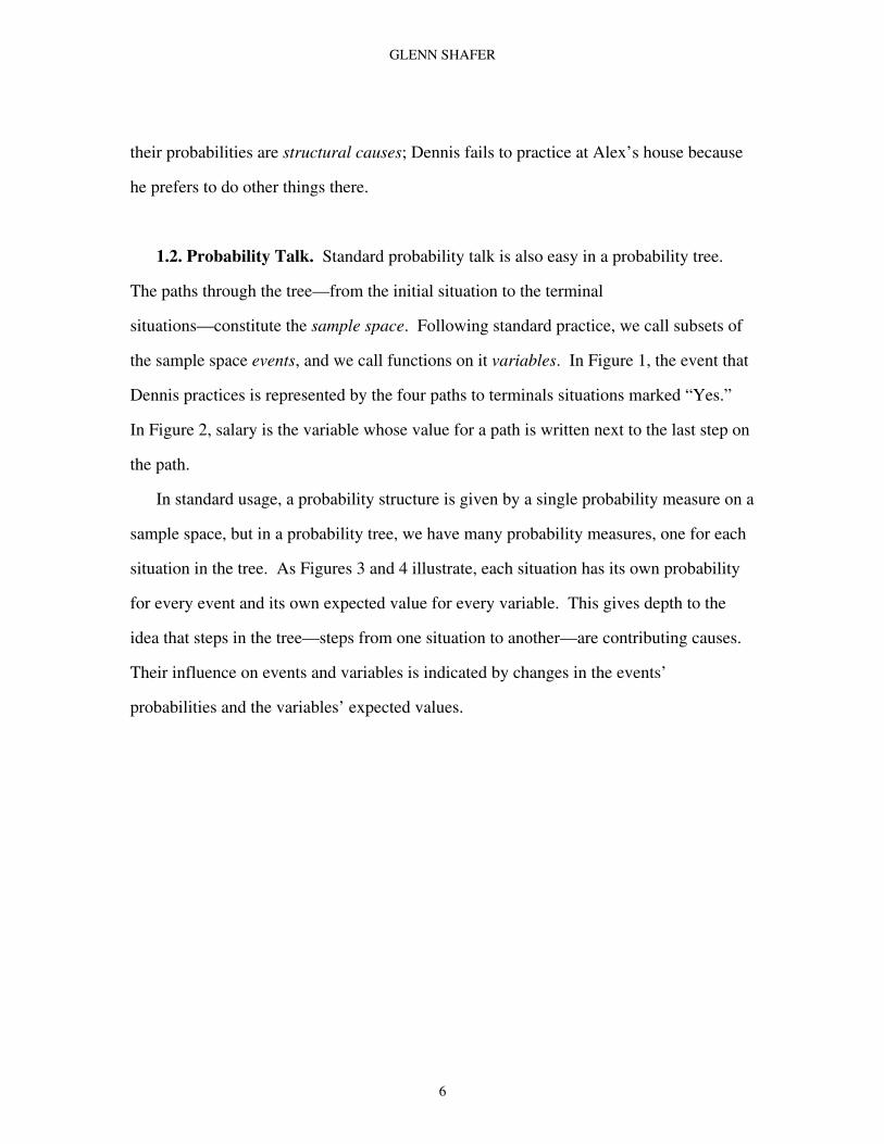
1.2. Probability Talk. Standard probability talk is also easy in a probability tree.

The paths through the tree—from the initial situation to the terminal

situations—constitute the sample space. Following standard practice, we call subsets of

the sample space events, and we call functions on it variables. In Figure 1, the event that

Dennis practices is represented by the four paths to terminals situations marked “Yes.”

In Figure 2, salary is the variable whose value for a path is written next to the last step on

the path.

In standard usage, a probability structure is given by a single probability measure on a

sample space, but in a probability tree, we have many probability measures, one for each

situation in the tree. As Figures 3 and 4 illustrate, each situation has its own probability

for every event and its own expected value for every variable. This gives depth to the

idea that steps in the tree—steps from one situation to another—are contributing causes.

Their influence on events and variables is indicated by changes in the events’

probabilities and the variables’ expected values.

GLENN SHAFER

7

Go to Sigmund's

Alex comes over

Alex does not come over

Stay at Dennis's

Go toAlex's Read Watch

television

Yes Yes NoNoYes

.5 .5

.4 .6

.4.611.8.2

.2 .4

No

1

Yes No

.1.9No

The probability that Dennis practices changes as nature moves through the tree.

Play soccer

Stay indoors

.4.6

.4

.47

.18

.36

.90

1

.76

.610.2

1 0 0

0 0

0 1 1 0

Figure 3 The probability that Dennis practices is shown in each situation.

.5 .5

.5 .5

Woman ManSex

Education

Salary

8 yrs 12 yrs

.95 .05

$8 $12

.05 .95

$8 $12

.5 .5

12 yrs 16 yrs

.95 .05

$12 $16

.05 .95

$12 $16

11.8

8 12 8 12 12 16 12 16

8.2 15.812.2

10 14

12

initial situation

Figure 4 The expected value of salary is shown in each situation.

We will use a notation that makes explicit the dependence of probabilities and

expected values on the situation:

• PS(E) is the probability of the event E in S.

GLENN SHAFER

8

• ES(X) is the expected value of the variable X in the situation S: ES(X) :=

ΣxPS(X=x).

• VarS(X) is the variance of X in S: VarS(X) := ES([X-ES(X)]2)

• CovS(X,Y) is the covariance of X and Y in S: CovS(X) := ES([X-ES(X)][Y-ES(Y)])

= ES(XY) - ES(X)ES(Y).

• PS(s) is probability of a step s in the situation S. (If s is below S, PS(s) is the product

of the branching probabilities on all the steps from S to and including s. If s is not

below S, PS(s) is zero.)

• ∆sX is the change in X’s expected value on step s. (If s goes from S to T, then ∆sX :=

ET(X) - ES(X).)

1.3. The Analysis of Variance. Analysis of variance is quite simple in probability

trees: we simply apportion VarS(X), the variance of X in S, among the steps of the tree.

The portion assigned to step s is

(1) PS(s) . (∆sX)2.

Figure 5 illustrates this decomposition for the example of Figure 4, with X as salary and

S as the initial situation.

GLENN SHAFER

9

Sex

Education

Salary

(.5).(.5).(8.2-10)2 = .81(.5).(.5).(11.8-10)2 = .81(.5).(.5).(12.2-14)2 = .81(.5).(.5).(15.8-14)2 = .81

11.8

8 12 8 12 12 16 12 16

8.2 15.812.2

10 14

12

.81 .81 .81 .81

2 2

(.5).(10-12)2 = 2(.5).(14-12)2 = 2

(.5).(.5).(.95).(8-8.2)2 = .0095(.5).(.5).(.05).(12-8.2)2 = .1805(.5).(.5).(.05).(8-11.8)2 = .1805(.5).(.5).(.95).(12-11.8)2 = .0095

(.5).(.5).(.95).(12-12.2)2 = .0095(.5).(.5).(.05).(16-12.2)2 = .1805(.5).(.5).(.05).(12-15.8)2 = .1805(.5).(.5).(.95).(16-15.8)2 = .0095

.0095.0095.1805

.1805 .0095.0095.1805

.1805

Figure 5 Apportioning the variance for salary. The two steps at which the sex of a child

is determined account for 50% of the initial variance of salary (4 out of 8 units). The four

steps at which education is determined account for another 40.5% (3.24 out of 8 units).

The steps at the bottom of the tree account for the remaining 9.5%.

The rule for apportioning variance among the steps of a probability tree generalizes to

covariance;

(2) PS(s) . ∆sX. ∆sY

is the portion of CovS(X,Y) we attribute to the step s. The following proposition

establishes that this does indeed define a decomposition.

Proposition 1. Suppose X and Y are variables in a probability tree, and S is a situation

in the tree. Then

(3) CovS(X,Y) = ∑s

PS(s).∆sX.∆sY ,

where the sum is over all steps in the tree.

GLENN SHAFER

10

Proof It suffices to consider the case where S is the initial situation, since any situation is

the initial situation in the subtree beginning with it.

In order to prove that (3) holds for the initial situation of every probability tree, we

can use induction on the number of nonterminal situations. If there is only one

nonterminal situation, as in Figure 6, then (3) reduces to

CovS(X,Y) = ∑ω

PS(ω).[X(ω)-ES(X)].[Y(ω)-ES(Y)] ,

where the sum is over the elements of the sample space. This is the usual definition of

covariance.

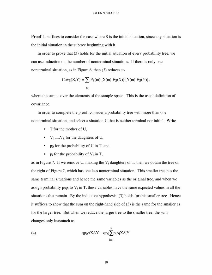
In order to complete the proof, consider a probability tree with more than one

nonterminal situation, and select a situation U that is neither terminal nor initial. Write

• T for the mother of U,

• V1,...,Vk for the daughters of U,

• p0 for the probability of U in T, and

• pi for the probability of Vi in T,

as in Figure 7. If we remove U, making the Vi daughters of T, then we obtain the tree on

the right of Figure 7, which has one less nonterminal situation. This smaller tree has the

same terminal situations and hence the same variables as the original tree, and when we

assign probability p0pi to Vi in T, these variables have the same expected values in all the

situations that remain. By the inductive hypothesis, (3) holds for this smaller tree. Hence

it suffices to show that the sum on the right-hand side of (3) is the same for the smaller as

for the larger tree. But when we reduce the larger tree to the smaller tree, the sum

changes only inasmuch as

(4) qp0∆X∆Y + qp0∑i=1

k

pi∆iX∆iY

GLENN SHAFER

11

is replaced by

(5) qp0∑i=1

k

pi[∆X+∆iX][∆Y+∆iY] ,

where q is the probability of T in the initial situation, ∆X := EU(X)-ET(X), and ∆iX :=

EVi(X)-EU(X). Multiplying the binomials in (5), we obtain

qp0∆X∆Y + qp0∑i=1

k

pi∆iX∆iY + qp0∆Y∑i=1

k

pi∆iX + qp0∆X∑i=1

k

pi∆iY .

And the last two terms are zero, because

EU(X) = ∑i=1

kpiEVi(X) and EU(Y) = ∑

i=1

kpiEVi(Y) . ♦♦♦♦

It should be emphasized that Equation (3) is a decomposition, not a representation of

CovS(X,Y) as a weighted average. The right-hand side is not a weighted average of the

products ∆sX.∆sY, because the “weights” PS(s) do not add to one.

PS(ω1)

S

ω1 ω2 ω3 ω4

PS(ω2) PS(ω3) PS(ω4)

Figure 6 When there is only one nonterminal situation, the steps constitute the sample

space, and the branching probabilities are the same as the probabilities of the elements of

the sample space in the initial situation.

GLENN SHAFER

12

p1

p2

U

V1 V2 V3

p3

p0

q2

q1

T

p0p1 p0p2

V1 V2 V3

p0p3

q2

q1

TRemove U.

Figure 7 The terms in (4) are the portions of the covariance associated with the four

steps marked on the left, while the terms in (5) are the portions associated with the three

steps marked on the right. In this example, q = q1q2.

1.4. Causal Conjecture. The rules for decomposing variance and covariance are rich

in implications. Here are a few of them:

Proposition 2. Suppose X and Y are variables in a probability tree.

1. If there is no step in the tree where X and Y both change in expected value, then X

and Y are uncorrelated in every situation (ES(XY) = ES(X)ES(Y) for every S).

2. If there is no step in the tree where the expected value of X goes up while the expected

value of Y goes down, and vice versa, then their correlation is nonnegative in every

situation (ES(XY) ≥ ES(X)ES(Y) for every S).

3. If there is no step in the tree where X and Y both change in probability, then X and Y

are independent in every situation (PS(X=x&Y=y) = PS(X=x)PS(Y=y) for every x, y,

and S).

Proof If X and Y never change in expected value on the same step, then ∆sX∆sY is zero

for every step s. It follows from (3) that for every situation S, CovS(X,Y) is zero, or

ES(XY) = ES(X)ES(Y).

GLENN SHAFER

13

Similarly, if ∆sX and ∆sY never have opposite signs, then their product is always

nonnegative, and it then follows from (3) that for every S, CovS(X,Y) ≥ 0, or ES(XY) ≥

ES(X)ES(Y).

Statement 3 follows from Statement 1, because the probability that X has a particular

value is the expected value of the variable that is equal to one when X takes that value

and zero otherwise. ♦♦♦♦

These statements illustrate the causal explanation of statistical patterns. If we observe

that X and Y are uncorrelated in many different situations, then we may conjecture that

they have no common causes—there are no steps in nature’s tree that affect them both. If

we observe that they are positively correlated in many different situations, then we may

conjecture that they consistently have common causes—the events that raise or lower the

expected level of one of them also raise or lower the expected level of the other.

We say that X and Y are causally uncorrelated when there is no step in nature’s tree

where they both change in expected value. Thus Statement 1 of Proposition 2 says that

causally uncorrelated variables are statistically uncorrelated. Similarly, we say that X

and Y are causally independent when there is no step in nature’s tree where they both

change in probability. Statement 3 says that causally independent variables are

statistically independent.

We can also provide a causal interpretation for regression coefficients. According to

standard theory, the coefficient of X in the linear regression of Y on X is

Cov(X,Y)Var(X) .

The following proposition reveals that this coefficient is a weighted average of the

relative changes in Y’s and X’s expected values on the different steps in nature’s tree.

GLENN SHAFER

14

Proposition 3. Suppose X and Y are variables in a probability tree, and S is a situation

in the tree. Then the regression coefficient of Y on X in S, CovS(X,Y)/VarS(X), is a

weighted average, over all the steps in the tree where X changes in expected value, of the

ratio of Y’s change in expected value to X’s. The weight of a step s is the probability of s

in S multiplied by the square of X’s change in expected value on s. In symbols:

(6)CovS(X,Y)VarS(X)

=

∑

s with ∆sX≠0

∆sY

∆sX. PS(s).(∆sX)2

∑

s with ∆sX≠0 PS(s).(∆sX)2

.

Proof Equation (6) follows immediately from (3) when we write its right-hand side in

the form

∑

s PS(s).∆sY.∆sX

∑

s PS(s).(∆sX)2

. ♦♦♦♦

If the ratios ∆sY/∆sX that the regression coefficient averages are quite disparate, then

the average is not very interesting, and we will say that the regression coefficient is

causally meaningless; it has no simple causal interpretation. But if these ratios are quite

similar, then we will feel that the average does have causal meaning. The most

interesting case is where the ratios are all equal. (Figure 8 gives an example.) In this

case, the regression coefficient will be the same in every situation, and we will say that

there is a stable causal relation between X and Y. This relation deserves a name; I have

proposed that we call X a linear sign of Y. The concept of linear sign is much more

general than the concepts of linear causality usually considered by statisticians and

philosophers (e.g., Freedman 1991, Humphreys 1989).

GLENN SHAFER

15

Education 8 12 16 8 12 16

Mom’s lottery ticket loses

Mom’s lottery ticket wins

1/2

1/31/3

1/3 1/31/3

1/3

IT

1/2

1/2 1/2 13/5 2/5 1/2 1/2 13/5 2/5

The expected value of Log10(Income) is shown in each situation.

2 3 4

3 1 6 41

$1,000 $10 $1,000,000 $10,000$10

4 5 6

5 3 8 63

$100,000 $1,000 $100,000,000 $1,000,000$1,000

3 5

4

S

Income

Figure 8 In this society, a person’s expected income goes up when the person gets more

education. In fact, when the expected value of Education changes, the expected value of

the logarithm (to the base 10) of Income changes by exactly one-fourth as much.

Consequently, the coefficient of Education in the linear regression of Log10(Income) on

Education is 1/4 in every situation where Education is not yet settled. The regression is

1+(1/4)Education in the initial situation I, (1/4)Education in S, and 2+(1/4)Education in

T.

Figure 9 summarizes our understanding of causality and statistical observation.

Correlation does not prove causality; we cannot deduce a causal relation from a statistical

association. But causality does imply statistical association, and hence statistical

association can give us grounds for conjecturing a causal relation. Causality can explain

correlation.

GLENN SHAFER

16

Logical Implication

Conjecture

CCaauussaa ll RReellaa tt iioonn

SSttaa tt ii ss tt ii ccaa ll RReellaa tt iioonn

Examples

X and Y are causally uncorrelated.

X and Y are statistically uncorrelated in all situations.

X and Y are causally independent.

X and Y are statistically independent in all situations.

X is a linear sign of Y.X and Y have the same correlation in all situations where X is indetrminate.

Figure 9 The dual connection between causal and statistical relations. More examples

are given in The Art of Causal Conjecture.

2. Refinement

Probability trees often seem naive, especially as part of a causal discussion, simply

because they necessarily leave aside many issues and factors that might be brought into

the discussion. The probability tree in Figure 1, for example, says nothing the factors that

decide whether Alex will come to Dennis’s house on a particular afternoon. How can the

tree be meaningful and valid if these factors are not taken into account?

The answer is that additional factors can be taken into account without falsifying the

assertions made in a particular probability tree. In other words, we can construct a more

refined tree that does take more into account but agrees with the assertions already made

GLENN SHAFER

17

in the original tree. In order to make a convincing case for probability trees, we

obviously need to show that such refinement really is possible. This is the purpose of this

section.

This section works is the same finite, graph-theoretical context as the preceding

section. In this context, as we will see, any refinement is a composition of elementary

refinements, each of which involve interpolation below a single situation. In the next

section, we will study refinement in the more general context of abstract event trees.

Once we have understood the idea of refinement, we will need to look again at the

causal concepts of the preceding section. As we will see, they need to be strengthened

slightly in order to for us to be sure that they will persist when a probability tree is

refined.

2.1. Elementary Refinements. When we suppose that a given probability tree

represents nature’s limited ability to predict, we are not supposing that nature is

blindfolded while each step is taken. When we suppose, for example, that nature gives

even odds on whether a woman will complete 12 years of education or only 8, we are

supposing only that these are nature’s odds at the moment when the woman is conceived

(and her sex is determined). As Figure 10 illustrates, nature’s odds on whether the

woman eventually chooses more education may change in the course of the woman’s

childhood.

GLENN SHAFER

18

.5 .5

8 yrs 12 yrs

.95 .05

$8 $12

.05 .95

$8 $12

Woman

.25 .75

8 yrs 12 yrs

.95 .05

$8 $12

.05 .95

$8 $12

Woman

.75 .25

8 yrs 12 yrs

.95 .05

$8 $12

.05 .95

$8 $12

Becomes a girl scout.

Does not become a girl scout.

.5 .5

Refinement

Figure 10 More detail on how the educational level of a woman is determined in the

society of Figure 2. The more refined tree does not contradict any causal assertions in the

original tree. It continues to assert, for example, that a woman with eight years of

education has only a 5% chance of earning $12.

We say that the probability tree on the right in Figure 10 is an elementary refinement

of the probability tree on the left. An elementary refinement involves interpolating a new

probability tree between a particular situation S and its daughters. The situation S may be

the initial situation, as in Figure 10, a later situation (as when the tree on the left of Figure

10 is considered as a subtree of Figure 2), or even a terminal situation (in this case, we

may prefer to say that we are adding a new tree below S rather than interpolating a tree

between S and its daughters). As Figure 11 illustrates, the interpolation proceeds as

follows:

1. If S is not terminal in the tree to be refined, remove the subtree below S.

2. Construct a new subtree below S.

3. If S was originally terminal, stop.

4. If S was not originally terminal, assign each terminal situation in the new subtree to

one of the original daughters of S, taking care to assign at least one to each original

GLENN SHAFER

19

daughter T, and taking care that the probabilities in S of the terminal situations

assigned to T add up to T’s usual probability in S.

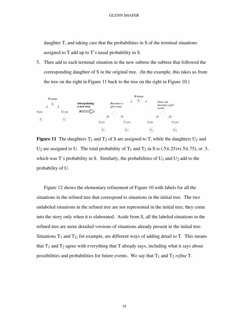
5. Then add to each terminal situation in the new subtree the subtree that followed the

corresponding daughter of S in the original tree. (In the example, this takes us from

the tree on the right in Figure 11 back to the tree on the right in Figure 10.)

.5 .5

8 yrs 12 yrs

Woman

.25 .75

8 yrs 12 yrs

Woman

.75 .25

8 yrs 12 yrs

Becomes a girl scout.

Does not become a girl scout.

.5 .5Interpolating a new tree

S

T U

T1 U1 T2 U2

S

Figure 11 The daughters T1 and T2 of S are assigned to T, while the daughters U1 and

U2 are assigned to U. The total probability of T1 and T2 in S is (.5)(.25)+(.5)(.75), or .5,

which was T’s probability in S. Similarly, the probabilities of U1 and U2 add to the

probability of U.

Figure 12 shows the elementary refinement of Figure 10 with labels for all the

situations in the refined tree that correspond to situations in the initial tree. The two

unlabeled situations in the refined tree are not represented in the initial tree; they come

into the story only when it is elaborated. Aside from S, all the labeled situations in the

refined tree are more detailed versions of situations already present in the initial tree.

Situations T1 and T2, for example, are different ways of adding detail to T. This means

that T1 and T2 agree with everything that T already says, including what it says about

possibilities and probabilities for future events. We say that T1 and T2 refine T.

GLENN SHAFER

20

.25 .75

.95 .05 .05 .95

.75 .25

.95 .05 .05 .95

.5 .5

Refinement

S

T U

T1 U1 T2 U2

S

P RQV

P1 R1Q1V1 P2 R2Q2V2

.5 .5

.95 .05 .05 .95

Figure 12 There are two situations in the more refined tree that are not represented in the

initial tree.

2.2. Combining Elementary Refinements. We say that one probability tree is a

refinement of another if it can be obtained by a sequence of elementary refinements.

Figure 13 shows a refinement that can be obtained by combining two elementary

refinements. In this example, the refinement does not provide more detail for situations

already present in the initial probability tree; it merely adds some new situations.

BorrowJaws.

BorrowJazz.

.5 .5

.2 .4

Jog. Go to library.

RefinementP

Q S

Read newspaper.

R

.4

.2 .8

Jog.Don’t jog.

P

Q

Read newspaper.

R S

Go to library.

.5 .5

Figure 13 The refinement reveals that the decision whether to jog is taken before a

choice is made between reading the newspaper and going to the library. It also shows

what can happen at the library.

GLENN SHAFER

21

2.3. Causal Relations Under Refinement. If the concepts that we defined in the

preceding section—causal uncorrelatedness, causal independence, and linear sign—are

really causal concepts, then they should not be affected by refinement of nature’s tree. If

we declare that two variables are causally uncorrelated (have no common causes) because

we see that they do not change in expected value on the same step of nature’s tree, then

we do not want to see this judgment contradicted when we take a closer look at nature’s

tree.

Unfortunately, the concepts as we have defined them do not quite have this invariance

under refinement. Figures 14 and 15 show the difficulty. In Figure 14, the events F and

G appear to be causally independent, for there is no step where they both change in

probability. But the refinement in Figure 15 shows that there are in fact steps where they

both change in probability.

.25

Ford sweeps in a.m.

Glenn sweeps in a.m.

Glenn sweeps in p.m.

Glenn cleans but does not sweep in p.m.

Ford sweeps in p.m.

Ford cleans but does not sweep in p.m.





.5.5Ford sweeps in p.m.


P(F) = .5P(G) = .5

P(F) = 1P(G) = 0

P(F) = 1P(G) = 1

.5.5.5.5.5.5

P(F) = 0P(G) = 1

P(F) = 0P(G) = 1

P(F) = 0P(G) = 0

P(F) = 1P(G) = 0

P(F) = 0P(G) = 0

P(F) = 1P(G) = 1

P(F) = 1P(G) = .5

P(F) = .5P(G) = 1

P(F) = 0P(G) = .5

P(F) = .5P(G) = 0

.25 .25 .25

Figure 14 Ford and Glenn clean their room twice a day. One of them cleans in the

morning; the other cleans in the afternoon. Sometimes cleaning requires sweeping,

sometimes not. We write F for the event that Ford eventually sweeps the room, and G for

the event that Glenn does. The probabilities of these events are shown for each situation.

(Alternatively, F and G can be thought of as variables, eventually taking the values zero

GLENN SHAFER

22

or one, and the numbers in the situations are then their expected values.) According to

the definition given in Section 1, the events F and G are causally independent, because

their probabilities do not change on the same step of the tree. (Equivalently, the variables

are uncorrelated, because their expected values do not change on the same step.)

.5.5Cookies in the mail.

No cookies in the mail.

Ford sweeps in a.m.

Glenn sweeps in a.m.



Ford sweeps in p.m.






.5.5Ford sweeps in p.m.


P(F) = .5P(G) = .5

.5.5

P(F) = .75P(G) = .75

.5.5

P(F) = .25P(G) = .25

P(F) = 1P(G) = 0

P(F) = 1P(G) = 1

.5.5.5.5.5.5

P(F) = 0P(G) = 1

P(F) = 0P(G) = 1

P(F) = 0P(G) = 0

P(F) = 1P(G) = 0

P(F) = 0P(G) = 0

P(F) = 1P(G) = 1

P(F) = 1P(G) = .5

P(F) = .5P(G) = 1

P(F) = 0P(G) = .5

P(F) = .5P(G) = 0

Figure 15 This refinement of Figure 14 reveals that when cookies come in the mail, the

probability of sweeping increases in both the morning and afternoon cleanings. The

refinement also shows that F and G are not really causally independent, for the step in the

tree where cookies come increases the probability of both.

The source of the difficulty in this example is clear. It is true that there are no steps in

Figure 14 where both events change in probability, but there are closely related

steps—alternative steps—where they do. The step from the initial situation in which

Ford sweeps in the morning does not change the probability of Glenn’s eventually

sweeping, but it has a sister that does. We obvious remedy is to rule this out.

Let us say that a situation in a probability tree influences a variable if the variable

changes in expected value on at least one of the possible steps immediately after that

situation. And let us then revise our earlier definitions as follows:

GLENN SHAFER

23

• X and Y are causally uncorrelated if in a sufficiently refined version of nature’s

probability tree, there is no situation that influences both X and Y.

• X and Y are causally independent if all functions of X are causally uncorrelated with

all functions of Y.

• X is a linear sign of Y with sign coefficient b if X and Y-bX are causally

uncorrelated.

We leave it to the reader to verify that these definitions require more than the earlier

definitions and that when they are satisfied by nature’s tree at one level of refinement,

they will be satisfied by nature’s tree at any greater level of refinement.

3. Abstract Event Trees

So far, our discussion has been based on a graph-theoretical conception of a tree.

Trees are rooted directed graphs without cycles. (For simplicity, we have put the root at

the top of our trees, directed all the arrows downward, and suppressed the arrowheads.)

This conception is useful. We can draw small trees of this kind, and even large ones have

straightforward computational representations. The intellectual tradition of probability is

hardly limited, however, to the finite and discrete. So we need to explore more general

ways of understanding probability trees. The first step, which we take in this section, is

to think abstractly about event trees. In later sections, we will look at refinement,

expectation, and probability in abstract event trees and at the more general concept of an

event space.

GLENN SHAFER

24

3.1. Event Trees Defined Abstractly. Abstractly, a tree is a special kind of partially

ordered set. (See, for example, Jech 1978.) In this spirit, let us say that an event tree is a

set Γ with a partial ordering3 precedes that has two properties:

Axiom T0 Γ has an element I such that I precedes S for all S in Γ.

Axiom T1 If S precedes U and T precedes U, then S precedes T or T precedes S.

We call the elements of an event tree situations. If S precedes T, we say that S precedes

or is a predecessor of T, and that T follows or is a successor of S. If S precedes T and

S ≠ T, we say S is a strict predecessor and T is a strict successor. If S precedes T or

T precedes S, we say S and T are sequenced. Thus Axiom T1 says that situations with a

common successor are sequenced.

The situation I mentioned in Axiom T0 is, of course, unique. We call it Γ’s initial

situation.

As we will see more clearly shortly, precedes carries a double meaning: S precedes T

means that

• T cannot happen unless S happens earlier (or at the same time, in which case S = T),

and

• T is possible (but has not already happened strictly earlier) whenever S happens.

3Recall that a binary relation is a partial ordering if it is reflexive, asymmetric, and

irreflexive. A binary relation is r is reflexive if S r S for all S, irreflexive if S r S for no S,

symmetric if S r T implies T r S, asymmetric if S r T and T r S implies S = T, and

transitive if S r T and T r U implies S r U.

GLENN SHAFER

25

More succinctly: S precedes T means that S is a prerequisite for T and allows T. Here we

are understanding S and T not only as situations but also as instantaneous events. The

instantaneous event S is the event that happens when and only when the event-tree

observer arrives in the situation S.

The following proposition shows that our abstract definition of an event tree is

consistent with the graph-theoretic conception.

Proposition 4.

1. Suppose (Γ,precedes) is a partially ordered set satisfying Axioms T0 and T1, and

suppose Γ is finite. Then the Hasse diagram of (Γ,precedes) is a finite directed tree, with

the initial situation as its root. (Figure 16 explains what is meant by the Hasse diagram

of a partially ordered set.)

2. Conversely, if we begin with a finite tree drawn as in the preceding sections, write

Γ for its set of situations, write I for the situation at the top, and write S precedes T

whenever there is chain of steps downward from S to T, then (Γ,precedes) is a partially

ordered set satisfying axioms T0 and T1.

Statement 1 may fail when Γ is infinite, because in this case, the journey from a situation

S to a later situation T may fail to consist of discrete steps. For example, if we conceive

of a different situation for each instant of time between S and T, then a step can always

be divided into smaller steps.

GLENN SHAFER

26

Partial OrderingP precedes PP precedes QP precedes RP precedes SP precedes TQ precedes QR precedes RR precedes SR precedes TS precedes ST precedes T

P

Q

S T

R

Represent graphically

Drop extra arrows

P

Q

S T

R

Figure 16 The Hasse diagram for a finite event tree. In general, to obtain the Hasse

diagram of a finite partially ordered set (Γ,precedes), we draw a graph with the elements

of Γ as nodes and an arrow from S to T whenever S precedes T, and then we delete the

arrow from S to T if there is a longer chain of arrows from S to T. (In the figure, we have

also deleted all arrowheads, on the understanding that steps are interpreted as arrows

pointing downwards.)

Here, as a counterpoint, is a simple and familiar example of an infinite event tree. Let

Γ be the set of all continuous real-valued functions that have closed intervals of real

numbers beginning at zero as domains and give the value zero to zero. In other words,

each element of Γ is a function S on some closed interval of the form [0,τ], with S(0) = 0.

Define the partial ordering precedes on Γ by saying that S precedes T if T extends S—i.e.,

if S is a function on [0,τ1], T is a function on [0,τ2], τ1 ≤ τ2, and T(t) = S(t) for all t from

0 to τ1, inclusive. The initial situation is the function that has only zero in its domain and

gives it the value zero.

3.2. Paths and the Sample Space. A path in an event tree is a maximal set of

sequenced situations—a set ω of situations such that any two elements of ω are

sequenced, and no other situation in the event tree is sequenced with them all. Every path

contains the initial situation. When a path contains a situation, it contains all the

GLENN SHAFER

27

situation’s predecessors. In a finite event tree, every path contains exactly one terminal

situation, and every terminal situation is in exactly one path. When a situation is in a

path, we say it goes through the path.

We speak also of paths from a particular situation: a path from S is a maximal set of

sequenced successors of S. Thus a path is the same as a path from the initial situation.

When S precedes T, we write [S,T] for the set of all situations that follow S and precede

T (this includes S and T), and we call [S,T] the closed interval between S and T.

The set of all paths is the event tree’s sample space, which we designate by Ω. A

subset of the sample space is a Moivrean event, and a function on the sample space is a

variable.

In Section 1, following the custom in probability theory, we used “event,” without

qualification, to mean what we now call a Moivrean event, in honor of Abraham De

Moivre. The adjective “Moivrean” is introduced here because we will need to distinguish

the Moivrean concept from other event concepts, including a concept we encountered a

moment ago—the concept of an instantaneous event represented by a situation.

3.3. Divergence. Two situations are divergent if they have no common successor.

By Axiom T1, this is equivalent to their not being sequenced. Divergent situations are

instantaneous events that cannot both happen. We write S divergent T when S and T are

divergent.

We say that S implies T and write S implies T when every successor of S (including S

itself) is sequenced with T. This means that S cannot happen unless T happens (sooner,

later, or at the same time).

We say that S foretells T and write S foretells T when S both precedes and implies T.

This is equivalent to the requirement that any path through S must later (or at the same

GLENN SHAFER

28

time) go through T (see Figure 17). It means that T cannot happen strictly earlier than S

but is inevitable (or happens at the same time) when S happens.

Like precedes, the binary relation foretells is a partial ordering on the event tree. The

binary relation implies is transitive and reflexive, but not asymmetric and hence not a

partial ordering. The binary relation divergent is symmetric.

S precedes but does not foretell T.

S

T

UR

S foretells T.

S

T

R

Figure 17 A situation S foretells a situation T if any path down the tree that passes

through S must later pass through T.

3.4. Clades. Let us call a nonempty set of divergent situations a clade. The

interpretation of individual situations as instantaneous events extends to clades: a clade Ξ

is the instantaneous event that happens when and only when the event-tree observer

arrives in a situation in Ξ. A clade, like a situation, can happen only once as the observer

moves through the tree. The various relations we have defined for situations also extend

to clades. Some of them (notably precedes and foretells) unpack in informative ways as

they extend.

If S is a situation, then S and S, the clade consisting of S alone, have the same

meaning when they are considered as instantaneous events. We call I, where I is the

initial situation, the initial clade.

GLENN SHAFER

29

When a path and a clade have a nonempty intersection, we say that the clade cuts the

path, and that the path goes through the clade.

When two clades Ξ and Φ are disjoint as sets, we write Ξ separate Φ. This means the

two clades cannot happen at the same time.

We say Ξ and Φ are divergent and write Ξ divergent Φ if each situation in Ξ is

divergent from each situation in Φ. This is equivalent to requiring that Ξ and Φ be

disjoint and their union be a clade. It means the two clades cannot both happen. It

generalizes divergence for situations: S divergent T if and only if S divergent T. If

Ξαα∈Α are divergent clades (if Ξα and Ξβ are divergent whenever α ≠ β), then the

union ∪α∈ΑΞα is a clade.

Here are six more binary relations for clades:

• Ξ prerequisite Φ (Ξ is a prerequisite for Φ) if every situation in Φ has a predecessor in

Ξ. This means that Ξ must happen before Φ can happen (though they may happen at

the same time).

• Ξ allows Φ (Ξ allows Φ) if every situation in Ξ has a successor in Φ. This means that

Φ is possible (but cannot already have happened strictly earlier) whenever Ξ happens.

It does not rule out Φ happening and Ξ not happening.

• Ξ implies Φ (Ξ implies Φ) if any path through Ξ also goes through Φ. This means that

Ξ cannot happen unless Φ happens (sooner, later, or at the same time).

• Ξ precedes Φ (Ξ precedes Φ) if Ξ prerequisite Φ and Ξ allows Φ. This means that Φ

cannot happen unless Ξ happens first or at the same time, and Φ is possible whenever

Ξ happens.

• Ξ foretells Φ (Ξ foretells or is a cause of Φ) if Ξ allows Φ and Ξ implies Φ. In other

words, if a path goes through Ξ, it goes through Φ at the same time or later. This

GLENN SHAFER

30

means that Φ cannot happen strictly earlier than Ξ but is inevitable (or happens at the

same time) whenever Ξ happens. It does not rule out Φ happening and Ξ not

happening.

• Ξ alw.foretells Φ (Ξ always foretells Φ) if Ξ precedes Φ and Ξ foretells Φ. In other

words, a path goes through Ξ if and only if it goes through Φ, and if it does go

through them, it goes through Ξ first or at the same time. This means that Φ cannot

happen unless Ξ happens first (or at the same time) and is inevitable (or happens at

the same time) whenever Ξ happens.

The relation implies is symmetric and transitive. The other five relations are partial

orderings. The dependencies among the six relations are clarified by the Venn diagram

in Figure 18. As this diagram indicates, Ξ alw.foretells Φ can be defined from the other

five relations in several ways. Instead of saying that it means Ξ precedes Φ and

Ξ foretells Φ, we can say, for example, that it means Ξ prerequisite Φ and Ξ implies Φ.

allows(1∪3∪4∪5)

prerequisite(2∪3∪4)

implies(4∪5∪6)

alw.foretells(4)

precedes(3∪4)

foretells(4∪5)

1

2 3 4 5 6

Figure 18 A Venn diagram for six binary relations on clades, thought of as sets of

ordered pairs of clades. A Venn diagram for three sets can have as many as seven

regions (not counting the region not in any of the sets), but the Venn diagram for

GLENN SHAFER

31

prerequisite, allows, and implies has only six, because Ξ prerequisite Φ and Ξ implies Φ

together imply Ξ allows Φ. By definition, precedes = prerequisite ∩ allows and

foretells = allows ∩ implies. We can obtain alw.foretells in several ways; it is the intersection

of either of the pair prerequisite,precedes with either of the pair implies,foretells.

When the clades Ξ and Φ are singletons, say Ξ = S and Φ = T, the six binary

relations reduce to three. The two relations S prerequisite T and S allows T are

equivalent to each other and hence to their conjunction, S precedes T. And

S foretells T and S alw.foretells T are equivalent. (See Figure 19.)

allows(1∪3∪4∪5)

prerequisite(2∪3∪4)

implies(4∪5∪6)

alw.foretells(4)

precedes(3∪4)

foretells(4∪5)

1

2 3 4 5 6

Figure 19 The six binary relations in Figure 16 reduce to three when we consider only

individual situations. In this case, prerequisite is equal to allows and hence to their

intersection, precedes. And alw.foretells and foretells are also equal.

We have defined precedes, foretells, and implies separately for clades and situations, but

the definitions agree: S precedes T if and only if S precedes T, and so on. Hence we

can ignore the distinction between S and S when talking about relations between

clades. The following equivalences are useful:

GLENN SHAFER

32

• Ξ prerequisite Φ if and only if Ξ prerequisite T for every T in Φ.

• Ξ allows Φ if and only if S allows Φ for every S in Ξ.

• Ξ implies Φ if and only if S implies Φ for every S in Ξ.

• Ξ foretells Φ if and only if S foretells Φ for every S in Ξ.

(The relations precedes and alw.foretells do not reduce in this way.) Of course, divergence

and disjointness reduce completely to relations between individual situations:

• Ξ divergent Φ if and only if S divergent T for every S in Ξ and T in Φ.

• Ξ separate Φ if and only if S ≠ T for every S in Ξ and T in Φ.

3.5. Cuts. When a clade Φ consists of successors of a situation S, and every path

through S also goes through Φ, we say that Φ is a cut of S.4 Intuitively, a cut of S is an

instantaneous event that cannot happen strictly before S happens or without S happening

but must eventually happen once S has happened. The clade S qualifies as a cut of S.

The condition S alw.foretells Φ is equivalent to Φ being a cut of S. The condition

Ξ foretells Φ is equivalent to every situation in Ξ having a cut in Φ. The condition

Ξ implies Φ is equivalent to every situation in Ξ having either a predecessor or a cut in Φ.

We refer to a cut of the initial situation simply as a cut. A cut is simply a clade that

cuts every path. Intuitively, it is an instantaneous event that must eventually happen (see

Figure 20).

4This differs from the definition of cut given in Section 11.2 of The Art of Causal

Conjecture.

GLENN SHAFER

33

I

Figure 20 A cut.

Any cut is a maximal clade—a clade that is not contained in a larger clade. In a finite

event tree, the converse is also true: any maximal clade is a cut. But as Figure 21

illustrates, a maximal clade may fail to be a cut in an infinite event tree. A clade cannot

always be enlarged to a cut.

S1

S2

S3

. . .

I

Figure 21 An event tree with one infinitely long path. This path does not go through the

clade S1,S2,..., which therefore is not a cut, although it is a maximal set of divergent

situations.

The following proposition tells us more about cuts.

GLENN SHAFER

34

Proposition 5.

1. If T is a successor of S, then there is at least one cut of S that contains T.

2. A set of sequenced successors of S is a path from S if and only if it intersects every

cut of S.

3. Suppose S is a situation, Φ is a set of divergent successors of S, and ω0 is a set of

sequenced successors of S. Suppose (1) no situation in Φ precedes a situation in ω0, and

(2) for every situation in Φ, there is a divergent situation in ω0. Then ω0 can be enlarged

to a path from S that does not go through Φ. (An example is provided by Figure 21, with

Φ equal to the clade S1,S2,... and ω0 an infinite subset of the infinitely long path.)

Proof 1. If ω is a path from S that does not go through T, then we can choose a situation

U in ω that is divergent from T, thus obtaining a clade T,U of successors of S that

contains T and cuts ω. More generally, if Ξ is a clade of successors of S that includes T,

and ω is a path from S not cut by Ξ, then we can construct another clade of successors of

S, say Ξ', that contains T and cuts both ω and all the paths from S already cut by Ξ.

(Choose a situation U divergent from T that cuts ω. If U is divergent from all the

situations in Ξ, then form Ξ' by adding U to Ξ. If U is sequenced with one or more

situations in Ξ, then it must be their strict predecessor, and we can form Ξ' by adding U

and removing these strict successors of U.) It follows by the axiom of choice that there

exists a clade of successors of S that contains T and cuts all paths from S.

2. The definition of cut tells us that a path from S intersects every cut of S. Suppose,

conversely, that ω is a set of sequenced successors of S that intersects every cut of S.

Consider any successor T of S not in ω. By Statement 1, there is a cut Ξ of S that

contains T, and by hypothesis, ω will contain a situation U that is also in Ξ. Since T and

U are both in Ξ, they are divergent, and hence T is not sequenced with all the situations in

GLENN SHAFER

35

ω. This shows that ω is a maximal set of sequenced successors of S—i.e., that it is a path

from S.

3. We begin by enlarging ω0 by adding all predecessors of its situations; the resulting

set ω1 will still be sequenced and satisfy conditions (1) and (2). Any situation sequenced

with all the situations in ω1 will follow all of them and hence will be divergent from Φ.

Hence it can be added to ω1 while preserving conditions (1) and (2). It follows by the

axiom of choice that ω0 can be enlarged to a path without adding any situation in Φ. ♦♦♦♦

3.6. Subordinate Event Trees. Suppose Γ is an event tree, with precedence ordering

precedes, and suppose Γ0 is a subset of Γ satisfying this axiom:

Axiom ST0 Γ0 contains a situation, say I0, that precedes all its other situations.

Then Γ0 will qualify mathematically an event tree with the inherited precedence ordering

(S precedes T in Γ0 if and only if S and T are in Γ0 and S precedes T in Γ). Axiom ST0

assures that Γ0 has an initial situation (not necessarily the same as Γ’s) and thus satisfies

Axiom T0, and precedes satisfies Axiom T1 in Γ0 because it does so in Γ. So we may call

Γ0 a subtree of Γ.

We need more than Axiom ST0, however, if we want to preserve relations of

necessity when we move between Γ and Γ0. Figure 17 illustrates the issue. The smaller

tree in that figure is a subtree of the larger tree, but as an event tree, it asserts that

S foretells T, which is not true in the larger tree. This suggests that we require the

following axiom:

Axiom ST1 If Ξ is a cut of I0 in Γ0, then Ξ is a cut of I0 in Γ.

GLENN SHAFER

36

When a subtree Γ0 satisfies Axiom ST1 as well as Axiom ST0, we say it is subordinate

to Γ. (More colloquially, it is a sub event tree.) The subtree in Figure 15 does not satisfy

ST1, because T is a cut of S in the smaller tree but not in the larger tree.

The following proposition clarifies the meaning of Axiom ST1.

Proposition 6. Suppose Γ is an event tree. And suppose the subset Γ0 of Γ satisfies

Axiom ST0 and hence is an event tree with the inherited precedence ordering, with I0 as

its initial situation. Then the following conditions are equivalent.

1. (Axiom ST1) If Ξ is a cut of I0 in Γ0, then Ξ is a cut of I0 in Γ.

2. If ω is a path in Γ, and ω∩Γ0 is nonempty, then ω∩Γ0 is a path in Γ0.

3. A nonempty set of situations in Γ0 is a path in Γ0 if and only if it is the intersection

with Γ0 of a path in Γ.

4. A set of situations in Γ0 is a cut of I0 in Γ0 if and only if it is a cut of I0 in Γ.

Proof 1. To show that Statement 1 implies Statement 2, consider a path ω in Γ, such

that ω∩Γ0 is nonempty. Since ω∩Γ0 is nonempty, goes through I0, and hence it goes

through every cut of I0 in Γ. It follows by Statement 1 that it goes through every cut of I0

in Γ0, and hence that it is a path in Γ0.

2. To show that Statement 2 implies Statement 1, consider a cut of I0 in Γ0. It will

cut every path in Γ0, and by Statement 2, this means that it will cut every path in Γ that

goes through I0 and so has a nonempty intersection with Γ0. Thus it is a cut of I0 in Γ.

3. Statement 3 obviously implies Statement 2. To show that the two are equivalent,

we must use Statement 2 to show that any path in Γ0 is the intersection with Γ0 of a path

in Γ. Let ω0 be a path in Γ0. Since ω0 is a set of sequenced situations in Γ0, the axiom of

GLENN SHAFER

37

choice assures that it can be enlarged to a path, say ω, in Γ. By Statement 2, ω∩Γ0 is a

path in Γ0. Since it contains ω0, it is equal to ω0.

4. Statement 4 obviously implies Statement 1. To complete the proof, notice that

Statement 3 implies that if the clade Ξ in Γ0 is a cut of I0 in Γ, then Ξ is a cut of I0 in Γ0.

As a cut of I0 in Γ, Ξ cuts every path in Γ that goes through I0. So by Statement 3, Ξ cuts

all paths in Γ0 and hence is a cut of I0 in Γ0. ♦♦♦♦

A subordinate event tree preserves all eight of the binary relations we have been

studying.

Proposition 7. Suppose Γ0 is an event tree subordinate to Γ. Suppose Ξ and Φ are

clades in Γ0. Then Ξ separate Φ in Γ0 if and only if Ξ separate Φ in Γ. And the analogous

statements hold for divergent, prerequisite, allows, implies, precedes, foretells, and alw.foretells.

Proof The disjointness of two sets is not affected, of course, by what larger set we place

them in. The relations divergent, prerequisite, and allows are preserved because they

depend only on relations of precedence between situations in the clades involved, and

these relations are inherited by Γ0 from Γ. By Statement 3 of Proposition 6, implies is

preserved. (Since Ξ and Φ are clades in Γ0, the condition that a path in Γ through Ξ also

go through Φ is equivalent to the same condition on the path’s intersection with Γ0.)

Finally, since precedes, foretells, and alw.foretells are defined in terms of prerequisite, allows,

and implies, they are also preserved. ♦♦♦♦

3.7. Humean Events. Thought of as an event, a situation S or a clade Ξ is

instantaneous; it is the arrival of the event-tree observer in S or Ξ. In discussions of

causality, we may also be interested in events that are not instantaneous. Such events can

GLENN SHAFER

38

be thought of as changes from one clade to another, and hence can be represented as pairs

of clades.

Formally, if Ξ precedes Φ, then we call the pair (Ξ,Φ) a Humean event. The clade Ξ is

its tail, and the clade Φ is its head. The head and tail may be identical; in this case the

Humean event is instantaneous. A Humean event is simple if its head and tail both

consist of single situations, initial if its tail is initial, inevitable if its head is a cut (in

which case its tail is also a cut), full if its tail implies its head (since the tail precedes the

head, this is the same as requiring that the tail cause the head, or that the tail be a full

cause of the head) and proper if the head does not include a cut of any of the situations

the tail. Two Humean events are divergent if their heads are divergent.

A simple Humean event (S,T) can be identified with the closed interval [S,T]. More

generally, any Humean event (Ξ,Φ) can be thought of as the set consisting of all closed

intervals that begin in Ξ and end in Φ.

A step from a situation S to a daughter T in a finite event tree is, of course, a closed

interval and hence a Humean event. But individual steps cannot play in a general theory

the special role they play when the event tree is finite. A daughter of S is a nearest strict

successor—a strict successor of S that has no strict predecessor that is also a strict

successor of S. In infinite event trees, where situations can have strict successors without

having nearest strict successors, we must look to Humean events to play the philosophical

and mathematical roles assigned to steps in Section 1: Humean events can represent

contingent causes, and as we will see in the next section, we can apportion a variable’s

variance among Humean events.

Like clades, Humean events retain their identity, in a certain sense, under refinement.

If ρ refines Γ to Γ*, then (Ξ,Φ) and (ρ(Ξ),ρ(Φ)) represent the same Humean event.

GLENN SHAFER

39

4. Martingales in Event Trees

Turning an event tree into a probability tree is simple in the finite case: we merely

add branching probabilities below each nonterminal situation. This approach does not

always work for infinite trees, for two reasons. One the one hand, there may be a

continuum of daughters. On the other hand there may be no daughters at all, as in the

example at the end of Subsection 3.1. How can we proceed?

The obvious answer is to shift attention from branching probabilities to expected

values. Expected values are assigned to situations, not to branches or steps, and

situations remain prominently present in our general theory of event trees. Instead of

thinking of a probability structure as a collection of branching probabilities, we think of it

as a linear space of functions—martingales, we shall call them—that assign numbers

(intuitively, expected values for numerical variables) to situations. Instead of

axiomatizing probabilities we axiomatize martingales.

This approach has a number of advantages. Most importantly, it points the way to

generalizations that allow probability to play a wider role in causal reasoning.

Traditionally, probability theory has insisted that probabilities be defined for all events,

and in the context of a finite event tree, this means that every step should have a

branching probability. But when we think of probability structure in terms of a linear

space of martingales, it is no longer natural to insist that the structure be complete in this

way. Each martingale in the structure is a declaration by the event-tree observer that

certain bets are fair—that they are among the bets the observer can make and expect to

break even—and the observer may have this kind of confidence in only a limited number

of bets. The events represented in the tree may include the observer’s own action, on

which it may not be sensible for her to bet. And when the event tree and the probability

structure represent nature, so that the martingales represent regularities that nature can

GLENN SHAFER

40

use for prediction, the extent of such regularities should be regarded as an empirical

question.

4.1. Martingales Defined. Let us call a numerical function on an event tree Γ a

process. A process µ is a martingale if it satisfies the following axiom:

Axiom M If S∈Γ, and Ξ is a cut of S, then there exist situations T1 and T2 in Ξ such that

µ(T1) ≤ µ(S) ≤ µ(T2).

If the event tree is finite, this is equivalent to saying that every nonterminal situation S

has daughters T1 and T2 such that µ(T1) ≤ µ(S) ≤ µ(T2).

For every number a, the process that is identically equal to a is a martingale. If µ is a

martingale, and a is a number, then aµ is a martingale. More generally, if µ is a

martingale, and f is a monotonic function, then f(µ) is a martingale. On the other hand, as

Figure 22 illustrates, the pointwise sum of two martingales is not necessarily a

martingale.

µµµµ µµµµ++++νννννννν

0 0 0

0 1 1 0 1 1

Figure 22 The processes µ and ν are martingales, but the process µ+ν is not.

The expected values of a numerical variable in a finite probability tree obviously

form a martingale. More precisely, if X is a variable in a finite probability tree, and we

define a process E(X) on the tree by setting

GLENN SHAFER

41

(7) E(X)(S) := ES(X),

then E(X) is a martingale. And the variable X is identified by E(X); its value on a path is

given by E(X)’s value on the terminal situation in that path. The abstract concept of

martingale does not depend, however, on the event tree having been made into a

probability tree by the addition of branching probabilities. Nor does a martingale

necessarily determine a variable.

We say a process is determinate in a situation S if all T that follow S are assigned the

same value as S by the process. We say a process is terminating if it is determinate in

some cut. If a process is terminating, then it determines a variable, whose value on each

path is the value the process eventually assumes on that path. We then say that the

process evaluates the variable, and we may think of the values of the process as

“expected values” of the variable. But we need not assume that a martingale always

settles down in this way.

4.2. Catalogs. We call a linear space of martingales on an event tree a catalog.

Catalogs provide the principal concept of probability structure in the remainder of this

article. Intuitively, a catalog represents all the gambling strategies an observer in the

event tree considers fair. The assumption that these strategies form a linear space derives

from the judgment that fairness is preserved under the formation of linear combinations.

If a given bet is fair, then it is fair to double it, and if two bets are individually fair, then it

is fair to combine them.

A catalog can contain at most one martingale evaluating a given variable. (If two

martingales in a catalog evaluate the same variable, then their difference, which is also in

the catalog and is therefore a martingale, will have the value zero everywhere by Axiom

M.) Whenever the catalog does contain a martingale that evaluates X, we write E(X) for

GLENN SHAFER

42

this martingale, and we call E(X) the expectation of X. We write ES(X) for E(X)(S), and

we call ES(X) the expected value of X in S.

In the case of a variable E that takes only the values zero and one (an event), we write

P(E) instead of E(E) and PS(E) instead of ES(E); we call the martingale P(E) the

probability of E, and we call the number PS(E) the probability of E in S. It often happens

that a catalog evaluates a variable X even though it does not evaluate all events of the

form X=x. When a catalog evaluates all events of the form X=x, we say it

probabilizes X.

In the case of a finite probability tree, the set of martingales E(X) | X is a variable,

where E(X) is given by (7), is a catalog. Such a catalog is maximal; since it already

contains a martingale evaluating every variable, it is not a subspace of a strictly larger

catalog. In general, we call a maximal catalog on an event tree a probability catalog.

While probability catalogs are interesting, smaller catalogs are also interesting, even

in the case of finite event trees. An important example is the finite decision tree, where

branching probabilities are provided for the branchings below chance situations, but not

for those below decision situations. Figure 23 gives an example. If we form martingales

by placing bets according to the odds given by the branching probabilities below chance

situations, then these martingales form a catalog, which we call the fair-bet catalog for

the decision tree. Each martingale in the catalog evaluates a variable, but not all

variables are evaluated by martingales in the catalog; the evaluated variables satisfy

linear constraints imposed by the fact that the martingales are all constant on the

daughters of each decision situation. For details, and for an analysis of the structure of all

catalogs on finite event trees, see Section 12.2 of The Art of Causal Conjecture.

GLENN SHAFER

43

No oil.Oil. No oil.Oil.

Drill.Don't drill.

Drill.Don't drill.

Take seismic soundings.

Drill.Forget the whole thing.

.5No oil.Oil.

Promising result.

Unpromising result.

.5 .25 .75

.4 .6 .1 .9

S T

U V

D1

D2 D3

Bet $10 on oil.

Bet $10 on oil.

Bet $10 on oil.

Bet $5 on promising result.

20

20 20

25 15

25 15

50 10

20

25 15

51051540

A Decision Tree A Martingale for the Decision Tree

Figure 23 The decision tree on the left is adapted from the problem of the

oil wildcatter in Raiffa (1968). There are branching probabilities for the

steps following the nonterminal chance situations S, T, U, and V, but no

branching probabilities following the decision situations D1, D2, and D3.

On the right is a martingale obtained by betting according to the branching

probabilities that are given.

In principle, any catalog can be enlarged to a probability catalog, and we might take

the view that a catalog that falls short of being a probability catalog is an incomplete

expression of opinion. This seems wrong-headed, however. If we take a constructive

view of probability judgment (Shafer and Tversky 1985), then we expect a person’s

probability opinions to be limited. And if we think of nature’s probabilities as reflecting

regularities in the world, then we have no reason to believe that such regularities are to be

found in every direction.

GLENN SHAFER

44

4.3. Stopping a Martingale. If µ is a martingale, and Ξ is a cut, then we write EΞ(µ)

for the process given by

EΞ(µ)(S) := µ(Ξ(S)),

where

Ξ(S) := S if T∈Ξ and S precedes T

R if R∈Ξ and R precedes S.

It is easy to see that EΞ(µ) is a martingale. We call it the expectation of µ in Ξ.

Intuitively, it is the result of stopping µ in Ξ. Figure 24 illustrates the idea.

11.8

8.2 8.2 8 12 14 14 14 14

8.2 1414

10 14

12

Figure 24 The martingale EΞ(µ), where µ is the martingale in Figure 4,

and Ξ is the cut in Figure 20. This martingale agrees with µ down to Ξ

and then remains unchanged the rest of the way down the tree.

The expectation of µ given Ξ is determinate in Ξ. If µ is determinate in Ξ, then

EΞ(µ) = µ. If Ξ and Φ are cuts and Ξ precedes Φ, then

EΞ(EΦ(µ)) = EΞ(µ),

an event-tree form of the rule of iterated expectation.

We call a catalog Μ Doob if it satisfies the following axiom:

GLENN SHAFER

45

Axiom V If µ∈Μ and Ξ is a cut, then EΞ(µ)∈Μ.

Probability catalogs are Doob, as are the fair-bet catalogs for decision trees. A catalog

that is not Doob can always be enlarged to one that is by adding all finite linear

combinations of its expectations and its elements. The idea of fairness could justify our

incorporating Axiom V into the definition of catalog, but since any linear space of

martingales can be enlarged in a canonical way to satisfy them, simplicity and

convenience is best served by calling any linear space of martingales a catalog.

4.4. Lower and Upper Probabilities. Consider an event tree Γ with a fixed Doob

catalog Μ. We say that a process µ on Γ is eventually less than or equal to a variable X

after S, and we write µ ≤↓S X, if in every path ω from S, there is a situation T such that

µ(U) ≤ X(ω) for all U following T. We define µ ≥↓S X similarly.

Given a variable X, we set

(8) ES-(X) := supµ(S) | µ∈Μ, µ ≤↓S X,

and we write E-(X) for the process given by E-

(X)(S) := ES-(X) . We call E-

(X) the lower

expectation of X, and we call ES-(X) the lower expected value of X in S.

Dual to the idea of lower expectation is the idea of upper expectation. The upper

expected value of X in S is

ES+

(X) := infµ(S) | µ∈Μ, µ ≥↓S X,

and the upper expectation of X is the process E+(X) given by E+

(X)(S) := ES+

(X) .

Notice that E-(X) = -E+

(-X).

The ideas of lower expectation and upper expectation are most easily understood in

terms of a house, an infinitely rich observer in the event tree, who is willing to make a bet

GLENN SHAFER

46

with another observer whenever that bet is in the catalog or is more favorable to herself

than one in the catalog. The lower expected value ES-(X) is the highest price the house

would pay for X in S, while the upper expected value ES+

(X) is the lowest price she

would charge for X in S. If the house were the only betting partner available to us, we

would think of ES-(X) as the scrap value of X in S, and of ES

+(X) as the cost of X in S.

Here are some informative properties of lower expectation.

Proposition 8.

1. The supremum in (8) is attained. In other words, for each S there is a martingale

µ in Μ such that µ ≥↓S X and µ(S) = ES-(X) .

2. E-(X) is a martingale.

3. E-(X) is the infimum of the expectations of X for the various probability catalogs

that contain Μ. There is a probability catalog containing Μ for which E-(X) is the

expectation of X.

4. If Ξ is evaluated by a martingale in Μ, so that the expectation E(X) exists, then

E-(X) = E(X).

(See Section 12.6 of The Art of Causal Conjecture. We leave it to the reader to formulate

the corresponding statements about upper expectation.) According to Statement 3, lower

expected values can be thought of as lower bounds. Upper expected values can similarly

be thought of as upper bounds. Different ways of completing the definition of the

branching probabilities in an event tree with a catalog produce different expected values

for X in S, and ES-(X) and ES

+(X) are tight lower and upper bounds, respectively, on

these expected values.

GLENN SHAFER

47

If we are in a position to enlarge the catalog to a probability catalog, by taking actions

that fix the branching probabilities, then it is appropriate to view lower expected and

upper expected values as bounds on expected values. Figure 25 illustrates the point. But

when it is not within our power to transform the tree into a probability tree by enlarging

its catalog, the idea that the lower and upper expectations are bounds should be treated

gingerly. There is no reason to say that there is an unknown expectation between the

lower expectation and upper expectation.

No oil.Oil. No oil.Oil.

Drill.Don't drill.

Drill.Don't drill.

Take seismic soundings.

Drill.Forget the whole thing.

.5No oil.Oil.

Promising result.

Unpromising result.

.5 .25 .75

.4 .6 .1 .9

S T

U V

D1

D2 D3

15

13 15

28 -2

28 -2

90 -10

0

-2 -2

-1288-1288

Figure 25 The upper expectation of a wildcatter’s payoff. We assume that it costs

$10,000 to drill and $2,000 to take seismic soundings, and that the wildcatter will earn

$100,000 if she finds oil. This gives the payoff X shown in the terminal situations. The

upper expected values of X are shown in the other situations. If the wildcatter wants to

choose the branching probabilities in the decision situations so as to maximize X’s

expected value in the initial situation, then the best she can do is EΩ+

(X) , or $15,000.

GLENN SHAFER

48

This is achieved by drilling in the initial situation with probability one. The choice of

branching probabilities for D2 and D3 is then immaterial, but in order to achieve the

upper expected value in D2, we should drill with probability one there. Any choice of

branching probabilities will achieve the upper expected value in D3.

When E is an event (a variable that takes only the values zero and one), we write

PS-(E) for ES

-(E) and call it the lower probability of E in S. Similarly, we write PS

+(E)

for ES+

(E) and call it the upper probability of E in S. The lower probability PS-(E) is the

highest price the house would pay for a contract that returns $1 if E happens, while the

upper probability PS+

(E) is the lowest price at which she would sell such a contract.

4.5. Causality. The theory of causality that we developed in Section 1 can be

extended to the general context of event trees with catalogs provided that we make

appropriate regularity assumptions. The simplest adequate assumption, perhaps, is that

each path in the event tree is compact in the interval topology. This means that for any

collection of closed intervals (see Subsection 3.2) that has ω as its union, there is a finite

subcollection that also has ω as its union.

Let us call a Humean event of the form (S,Ξ), where Ξ is a cut of S, an experiment,

and let us call the set of situations

T | S precedes T and there exists U∈Ξ such that T precedes U

the scope of the experiment (S,Ξ). Let us call a collection of experiments a cover if the

union of the scopes is equal to the entire event tree.

We say that an experiment forbears a martingale if the martingale has the same value

on all situations in the experiment’s scope. We say that two martingales are uncorrelated

if there exists a cover, every experiment in which forbears at least one of the two

GLENN SHAFER

49

martingales. The following proposition is about uncorrelated martingales is illustrated by

Figure 26.

Proposition 9. Suppose µ and ν are uncorrelated martingales. Then µ+ν and µν are

martingales. More generally, f(µ,ν) is a martingale whenever f(x,y) is monotonic in both

its arguments.

µµµµ

.5

1

1 1

0

0 0

νννν

.5

.5

1 0

.5

1 0

µµµµ++++νννν

1

1.5

2 1

.5

1 0µµµµνννν

.25

.5

1 0

0

0 0

Figure 26 Two uncorrelated martingales, their sum, and their product.

We say that two variables Y and Z are causally uncorrelated if they are evaluated and

the martingales evaluating them are uncorrelated. The next proposition then spells out

within in this general theory the fact, which we took notice of for finite probability trees

in Section 1, that causal uncorrelatedness implies uncorrelatedness in the usual sense.

GLENN SHAFER

50

Proposition 10. Consider an event tree with a Doob catalog Μ.

1. If µ and ν are uncorrelated martingales in Μ, then µν is in Μ.

2. If X and Y are uncorrelated variables, then the product XY is evaluated, and E(XY)

= E(X)E(Y).

From the idea of causal uncorrelatedness, we can also construct the other causal ideas

that we mentioned in Section 1. For example, we say that two variables X and Y are

causally independent if they are probabilized and X=x is uncorrelated with Y=y for

all x and y, and we can then prove that causally independent variables are independent in

the usual sense.

4.6. Limit Theorems. The idea of lower probability is important because it allows us

to formulate the traditional limit theorems of probability theory, which assert that various

things are almost certain to happen in a long run of trials. We simply interpret “almost

certain” as “with very high lower probability.”

An example of this approach is provided by the following version of the law of large

numbers.

Proposition 11. For any positive real number K (no matter how large) and any positive

real numbers ε and δ (no matter how small), there exists an integer N such that if n≥N

and X1,X2,..,Xn are causally uncorrelated variables in an event tree with a Doob catalog,

all the Xi have value zero in the initial situation I, all are bounded by K, and X_

is their

average, then PI-(|X

_|≤δ) ≥ 1-ε.

GLENN SHAFER

51

The law of large numbers has the same significance in our theory as it does in standard

probability theory. It implies that if situations are replicated as nature moves through her

tree, we can estimate nature’s probabilities in these situations from observed frequencies.

Other limit theorems, especially the law of large numbers and the law of the iterated

logarithm, and have been treated from essentially the point of view taken here by Vovk

(1993a,b).

5. Refinement of Abstract Event Trees

How can we describe abstractly the relation between an event tree and a refinement?

The examples in Section 2 suggest that we specify, for each situation S in the original

tree, the situations in the refinement that agree with S, in the sense that they represent the

same instantaneous event, possibly describing it in more detail. These situations are

divergent—i.e., they form a clade, say ρ(S) in the refinement. If we set ρ(Ξ) :=

∪S∈Ξρ(S) when Ξ is a clade in the original tree, then ρ(Ξ) is also a clade in the

refinement, consisting of situations that agree with and possibly add more detail to some

situation in Ξ. The mapping from clades to clades thus defined fully specifies the

relationship between the two event trees.

5.1. An Axiomatization of Refinement. Formally, let us say that a mapping ρ from

clades in an event tree Γ to clades in an event tree Γ* refines Γ to Γ* if it satisfies the

following axioms:

GLENN SHAFER

52

Axiom R0 Ξ is initial if and only if ρ(Ξ) is initial.5

Axiom R1 Ξ separate Φ if and only if ρ(Ξ) separate ρ(Φ).

Axiom R2 Ξ divergent Φ if and only if ρ(Ξ) divergent ρ(Φ).

Axiom R3 Ξ prerequisite Φ if and only if ρ(Ξ) prerequisite ρ(Φ).

Axiom R4 Ξ allows Φ if and only if ρ(Ξ) allows ρ(Φ).

Axiom R5 Ξ implies Φ if and only if ρ(Ξ) implies ρ(Φ).

Axiom R6 If Ξαα∈Α are divergent clades in Γ, then ρ(∪α∈ΑΞα) = ∪α∈Αρ(Ξα).

When ρ refines Γ to Γ*, we say Γ* is a refinement of Γ, and Γ is a coarsening of Γ*.

Axioms R0-R6 are easy to justify on the understanding that (1) a clade represents the

instantaneous event that the observer arrives in a situation in the clade, and (2) Ξ and

ρ(Ξ) represent the same instantaneous event. From this perspective, the axioms merely

say that the meaning of various relations among instantaneous events (being divergent,

one being a prerequisite for the other, etc.) is not affected by the choice of an event tree in

which to represent the events.

We will abbreviate ρ(S) to ρ(S). By Axiom R2, the clades ρ(S) are all disjoint.

When S* is an element of ρ(S), we say S* refines or is refinement of S, and S coarsens or

is a coarsening of S*.

Given a subset γ* of Γ*, we write ρ-1(γ*) for the subset of Γ consisting of all

coarsenings of situations in γ*.

The following proposition clarifies some aspects of refinement.

5In other words, ρ(I) = I*, where I and I* are the initial situations in Γ and Γ*,

respectively.

GLENN SHAFER

53

Proposition 12. Suppose ρ refines Γ to Γ*, and suppose Ξ and Φ are clades in Γ.

1. ρ(Ξ) = ∪S∈Ξρ(S).

2. Ξ = Φ if and only if ρ(Ξ) = ρ(Φ).

3. Ξ precedes Φ if and only if ρ(Ξ) precedes ρ(Φ).

4. Ξ foretells Φ if and only if ρ(Ξ) foretells ρ(Φ).

5. Ξ alw.foretells Φ if and only if ρ(Ξ) alw.foretells ρ(Φ).

6. Suppose S coarsens S*, T coarsens T*, and S* precedes T*. Then S precedes T.

7. Φ contains a cut of S if and only if ρ(Φ) contains a cut of every refinement of S.

8. Suppose S* and a successor T* refine situations in Γ. Then T* can be extended to

a cut of S* consisting of situations that refine situations in Γ.

9. The event tree, say Γ*0, obtained by omitting from Γ* all situations that do not

refine situations in Γ, is subordinate to Γ*. Moreover, the mapping ρ, thought of as a

mapping from clades of Γ to clades of Γ*0, refines Γ to Γ*0.

10. Suppose T coarsens T* and S precedes T. Then there exists a situation S* that

refines S and precedes T*.

11. Suppose S coarsens S* and S precedes T. Then there exists a situation T* that

follows S* and refines T.

12. Suppose S coarsens S*. Then (1) if ω* is a path from S*, then ρ-1(ω*) is a path

from S, and (2) if ω is a path from S, then ω = ρ-1(ω*) for some path ω* from S*.

13. Suppose S coarsens S*, and Φ is a cut of S. Then Φ = ρ-1(Φ*) for some cut Φ*

of S*.

Proof 1. Statement 1 is a special case of Axiom R6.

2. Since the ρ(S) are disjoint, by Axiom R1, Statement 2 follows from Statement 1.

3. Statement 3 follows from Axioms R3 and R4.


GLENN SHAFER

54


6. By Axiom R2, S and T must be sequenced rather than divergent. So either S

precedes T or T precedes S. If T precedes S, then by Axiom R3, there exists a refinement

T*2 of T that precedes S* and hence T*; since ρ(T) is a clade, this implies that T*2 = S*

= T*; and so by Axiom R1, S = T. Hence S precedes T.

7. Recall that (1) Φ containing a cut of Ξ is equivalent to Ξ foretells Φ and (2) Ξ

foretells Φ is equivalent to S foretells Φ for all S in Ξ. Using these equivalences and

Statement 4, we see that Φ containing a cut of S is equivalent to S foretells Φ, which is

equivalent to ρ(S) foretells ρ(Φ), which is equivalent to ρ(Φ) containing a cut of ρ(S),

which is equivalent to ρ(Φ) containing a cut of S* for every S* in ρ(S).

8. Let S and T be the situations refined by S* and T*, respectively. By Statement 6,

S precedes T. By Proposition 5, T can be extended to a cut Φ of S. By Statement 7, ρ(Φ)

contains a cut of S*. Since T* is a successor of S* and is in ρ(Φ), the maximality of the

cut requires that it contain T*.

9. In order to show that Γ*0 is subordinate to Γ*, it suffices to consider a path ω in

Γ* and to show that ω∩Γ*0 is a path in Γ*0. To show that ω∩Γ*0 is a path in Γ*0, it

suffices to consider a situation S* in Γ*0 that is sequenced with all the situations in

ω∩Γ*0 and to show that it is in ω. We write S for the situation in Γ that S* refines, and

we consider two cases: (1) S* has a successor in ω∩Γ*0, and (2) S* has no successor in

ω∩Γ*0. In case (1), S* is in ω because it has a successor in ω. In case (2), S* is a

successor of all the situations in ω∩Γ*0. By Statement 8, S* can be extended to a cut

consisting of situations in Γ*0. Choose such a cut, and let T* be the situation it has in

common with ω. Then T* is a predecessor of S* and yet is in the same cut as S*. This

means that T* = S*, so that S* is in ω.

GLENN SHAFER

55

Since the mapping ρ is not altered, Axioms R0, R1, and R6 continue to hold.

Omitting situations from an event tree does not alter any precedence relations for

situations that remain. From this we can see first that it does not alter the set of

prerequisite relations or the set of allows relations among clades that remain, then that it

does not alter the set of precedes relations, and then that it does not alter the set of divergent

relations. Hence Axioms R2, R3, and R4 continue to hold under ρ0.

The case of implies relations is slightly more subtle. In general, omitting situations

from an event tree cannot destroy implies relations, but it can introduce new ones. So we

must consider the case where ρ(Ξ) implies ρ(Φ) does not hold in Γ*. Is it possible that

when we omit all the situations that do not refine situations in Γ, we omit all the

successors of ρ(Ξ) divergent from ρ(Φ), so that ρ(Ξ) implies ρ(Φ) holds in Γ*0? No.

Since Ξ implies Φ does not hold in Γ, there is a successor T of Ξ that is divergent from Φ.

Any refinement T* of T will be a successor of ρ(Ξ) divergent from ρ(Φ).

10. Statement 10 follows from Axiom R3.

11. Statement 11 follows from Axiom R4.

12. By Statement 6, any two situations in ρ-1(ω*) are sequenced. So in order to

show that ρ-1(ω*) is a path from S, it suffices to consider a successor T of S that is

sequenced with all the situations in ρ-1(ω*) and show that T is in ρ-1(ω*). We consider

two cases. (1) T has a successor U in ρ-1(ω*). Let U* be U’s refinement in ω*.

Statement 10 tells us that T has a refinement T* that precedes U* and hence is also in ω*.

So T is in ρ-1(ω*). (2) T does not have a successor in ρ-1(ω*); all the situations in

ρ-1(ω*) precede T. In this case, choose a cut Φ of S containing T. By Statement 7, ρ(Φ)

contains a cut of S*, and hence the path ω* goes through ρ(Φ); ρ-1(ω*) and Φ have a

situation in common. Since T is sequenced with all the situations in ρ-1(ω*) and

GLENN SHAFER

56

divergent from all the other situations in Φ, none of the other situations in Φ can be in

ρ-1(ω*). So T is in ρ-1(ω*).

Now suppose ω is a path from S. Choose a situation T in ω. Using Statement 11,

choose a situation T* that follows S* and refines T. Let ω*0 be the predecessors of T*.

Then ω*0 is a set of sequenced successors of S*, and by Statements 6 and 10, ρ-1(ω*0) is

the subset of ω consisting of all situations that follow S and precede T. For any successor

T1 of T in ω, we can repeat this exercise, extending ω*0 to a set ω*1 of sequenced

successors of S* that includes a refinement of T1, so that ρ-1(ω*1) is the subset of ω

consisting of all situations that follow S and precede T1. By the axiom of choice, we can

enlarge ω*0 to a set ω*∞ of sequenced successors of S* such that ρ-1(ω*∞) = ω. Again

by the axiom of choice, we can enlarge ω*∞ to a path ω* from S*, since this will only

involve adding successors that do not refine situations in Γ, we will have ρ-1(ω*) = ω..

13. By Statement 7, ρ(Φ) contains a cut of S*. Let Φ* be this cut. In order to show

that Φ = ρ-1(Φ*), we must show that Φ* contains a refinement of an arbitrary situation T

in Φ. There is a path from S through T, and by Statement 12, this path is equal to ρ-1(ω*)

for some path from S*. Let T1* be the refinement of T in ω*, and let T2* be the situation

where Φ* cuts ω*. Since they are both in ω*, T1* and T2* are sequenced. Since they are

both in ρ(Φ), they must be divergent or equal. So they are equal; Φ* contains a

refinement of T. ♦♦♦♦

GLENN SHAFER

57

coarsens

coarsens

precedes

S

T

precedes

S*

T*If the relations in bold hold, then the relation in outline holds.

If the relations in bold hold, then there exists S* such that the relations in outline hold.

coarsens

coarsens

precedes

S

T

precedes

S*

T*If the relations in bold hold, then there exists T* such that the relations in outline hold.

coarsens

coarsens

precedes

S

Tprecedes

S*

T*

Figure 27 Statements 6, 10, and 11 of Proposition 12.

5.2. An Alternative Axiomatization. Axioms R0-R6 constitute only one way of

axiomatizing refinement; there are many others, some much more austere. For example,

instead of thinking of refinement from Γ to Γ* as a mapping that assigns a clade in Γ* to

each clade in Γ, we can step back to thinking of it as a mapping that assigns a clade of

situations ρ(S) in Γ* to each situation S in Γ, and we can adopt the following axioms:

Axiom R0' ρ(I) = I*.

Axiom R1' All the ρ(S) are disjoint from each other.

Axiom R2' If S divergent T, then ρ(S) divergent ρ(T).

Axiom R3' If S precedes T, then ρ(S) precedes ρ(T).

Axiom R4' Suppose Φ is a clade in Γ and S* is in ρ(S). Then if Φ is a cut of S if and

only if ∪T∈Φρ(T) contains a cut of S*.

As the following proposition shows, Axioms R0'-R4' are equivalent to Axioms R0-R6.

Proposition 13.

GLENN SHAFER

58

1. Suppose ρ is a mapping from clades in Γ to clades in Γ* that satisfies Axioms R0-

R6. Define a new mapping ρ from situations in Γ to clades in Γ* by setting ρ(S) :=

ρ(S). Then this new mapping ρ satisfies Axioms R0'-R4'.

2. Suppose ρ is a mapping from situations in Γ to clades in Γ* that satisfies Axioms

R0'-R4'. Define a new mapping ρ from clades in Γ to sets of situations in Γ* by setting

ρ(Ξ) := ∪S∈Ξρ(S). Then ρ(Ξ) is a clade in Γ* for every clade Ξ in Γ, and ρ satisfies

Axioms R0-R6.

Proof 1. Axiom R0' follows from Axiom R0. Axiom R1' follows from Axiom R1.

Axiom R2' follows from Axiom R2. Axiom R3' follows Statement 3 of Proposition 12.

Axiom R4' follows from Statement 7 of Proposition 12.

2. It follows from Axiom R2' that each ρ(Ξ) is a clade. Axiom R0 follows from

Axioms R0' and R1'. Axiom R1 follows from Axiom R1'.

It follows from Axiom R2' that if Ξ is divergent from Φ, then ρ(Ξ) is divergent from

ρ(Φ). On the other hand, if Ξ is not divergent from Φ, then

there are situations S in Ξ and T in Φ that are sequenced, and hence, by Axiom R3', there

are situations S* in ρ(S) and T* in ρ(T) that are sequenced, whence ρ(Ξ) is divergent

from ρ(Φ). This establishes Axiom R2.

Suppose Ξ prerequisite Φ. Consider a situation T* in ρ(Φ). Let T be the situation in

Φ that coarsens T*. By the assumption Ξ prerequisite Φ, T has a predecessor S in Ξ. By

Axiom R3', T* has a predecessor, say S*, in ρ(Ξ). Since T* was an arbitrary situation in

ρ(Φ), this establishes that ρ(Ξ) prerequisite ρ(Φ).

Now suppose ρ(Ξ) prerequisite ρ(Φ). Consider a situation T in Φ. Choose a situation

T* in ρ(T). Let S* be T*’s predecessor in ρ(Ξ), and let S be the situation in Ξ that

coarsens S*. By Axiom R2', S and T must be sequenced. If T were to precede S, then by

Axiom R3' we would have ρ(T) precedes ρ(S), which would imply the existence of a

GLENN SHAFER

59

situation T2* in ρ(T) such that T2* precedes S* precedes T*, and since ρ(T) is a clade, this

would imply that S* = T*, whence (Axiom R1') S = T. So S precedes T. This establishes

Ξ prerequisite Φ and hence completes the derivation of Axiom R3.

Suppose Ξ allows Φ. Consider a situation S* in ρ(Ξ). Let S be the situation in Ξ that

coarsens S*. Then S has a successor T in Φ. By Axiom R3', S* has a successor, say T*,

in ρ(Φ). This establishes ρ(Ξ) allows ρ(Φ).

Now suppose ρ(Ξ) allows ρ(Φ). Consider a situation S in Ξ. Choose a situation S* in

ρ(S). Let T* be a successor of S* in ρ(Φ), and let T be the situation in Φ that coarsens

T*. By the same argument we used in the paragraph before last, S precedes T. This

establishes Ξ allows Φ and hence completes the derivation of Axiom R4.

Suppose Ξ implies Φ. Consider a situation S* in ρ(Ξ). Let S be the situation in Ξ that

coarsens S*. Then S has either a predecessor or a cut in Φ. If S has a predecessor in Φ,

then by Axiom R3', S* has a predecessor in ρ(Φ). If S has a cut in Φ, then by Axiom

R4', S* has a cut in ρ(Φ). This establishes that ρ(Ξ) implies ρ(Φ).

Now suppose ρ(Ξ) implies ρ(Φ). Consider a situation S in Ξ. Choose a situation S* in

ρ(S). Then S* has either a predecessor or a cut in ρ(Φ). If S* has a predecessor in ρ(Φ),

then by a previous argument, S has a predecessor in Φ. If S* has a cut in ρ(Φ), then by

Axiom R4', S has a cut in Φ. This establishes Ξ implies Φ and hence completes the

derivation of Axiom R5.

Finally, Axiom R6 follows from the definition ρ(Ξ) := ∪S∈Ξρ(S). ♦♦♦♦

For further ways of axiomatizing refinement, see Section 13.3 of The Art of Causal

Conjecture.

GLENN SHAFER

60

5.3. Consistency with Finite Refinement. The following proposition assures us that

the concept of refinement contained in Axioms R0-R6 agrees, in the finite case, with the

concept of refinement developed in Section 2.

Proposition 14.

1. Suppose Γ and Γ* are finite event trees, and Γ* is a refinement of Γ in the sense of

Section 2. For each situation S in Γ, let ρ(S) be the set of situations in Γ* that refine S.

For each clade Ξ in Γ, set

ρ(Ξ) = ∪S∈Ξρ(S).

Then ρ(Ξ) is always a clade in Γ*, and the mapping ρ satisfies Axioms R0-R6.

2. Suppose ρ refines Γ to Γ* in the sense of this section, and suppose Γ and Γ* are

finite. Then ρ is a composition of elementary refinements of the kind described in Section

2.

Proof 1. Statement 1 is obviously satisfied by an elementary refinement. To see that it

is also satisfied by a composition of elementary refinements, it suffices to notice that

composition of refinements means composition of the corresponding mappings: if ρ1

represents the refinement from Γ to Γ*, and ρ2 represents the refinement from Γ* to Γ**,

then ρ2°ρ1 represents the refinement from Γ to Γ**. It is obvious from the form of the

axioms that they are preserved by such composition.

2. We will prove Statement 2 using induction on the number of nonterminal

situations in Γ*. Suppose first that there is only one nonterminal situation in Γ*, which is

therefore the initial situation and has all the terminal situations as its daughters. And

consider two cases: (1) there is no situation S in Γ such that ρ(S) contains a terminal

situation in Γ*, and (2) there is such a situation S.

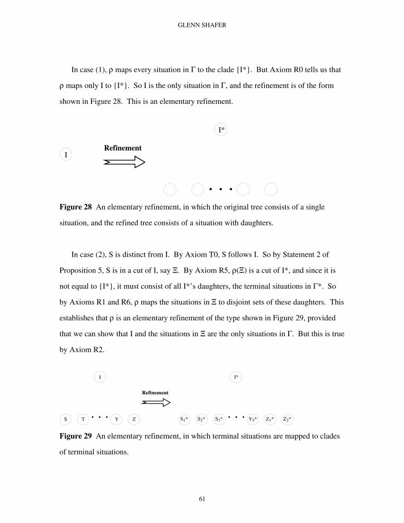
GLENN SHAFER

61

In case (1), ρ maps every situation in Γ to the clade I*. But Axiom R0 tells us that

ρ maps only I to I*. So I is the only situation in Γ, and the refinement is of the form

shown in Figure 28. This is an elementary refinement.

I*

I

. . .

Refinement

Figure 28 An elementary refinement, in which the original tree consists of a single

situation, and the refined tree consists of a situation with daughters.

In case (2), S is distinct from I. By Axiom T0, S follows I. So by Statement 2 of

Proposition 5, S is in a cut of I, say Ξ. By Axiom R5, ρ(Ξ) is a cut of I*, and since it is

not equal to I*, it must consist of all I*’s daughters, the terminal situations in Γ*. So

by Axioms R1 and R6, ρ maps the situations in Ξ to disjoint sets of these daughters. This

establishes that ρ is an elementary refinement of the type shown in Figure 29, provided

that we can show that I and the situations in Ξ are the only situations in Γ. But this is true

by Axiom R2.

Refinement

. . .

I*

S2* Z1*S1* Z2*S3* Y5*. . .

I

S ZT Y

Figure 29 An elementary refinement, in which terminal situations are mapped to clades

of terminal situations.

GLENN SHAFER

62

Now suppose Statement 2 holds for refinements with n or fewer nonterminal

situations, and suppose Γ* has n+1 nonterminal situations.

We consider three cases: (1) ρ(S) is always a single situation, and every situation in

Γ* refines a situation in Γ, (2) at least one situation in Γ* does not refine a situation in Γ,

and (3) every situation in Γ* refines a situation in Γ, and at least one pair of distinct

situations in Γ* refine the same situation in Γ.

In case (1) ρ maps Γ one-to-one and onto Γ*, and by Axiom R3 (or R4), it also

preserves precedence, so that it is the identity mapping from the partially ordered set Γ to

itself, and this qualifies as an elementary refinement.

In case (2), choose a situation Z* in Γ* that does not refine a situation in Γ. Let P* be

the nearest predecessor of Z* that refines a situation in Γ. By Statement 8 of Proposition

8, P* either has no strict successors that refine situations in Γ or has a whole cut of them.

In the first case, we may omit the strict successors of P* to obtain a smaller refinement of

Γ, and the addition of the strict successors constitutes a further elementary refinement, so

that the proof by induction is complete. In the second case we may choose the cut so that

all the situations strictly between P* and the cut do not refine elements of Γ, and Z* will

be one of these. Omitting these situations again produces a smaller refinement of Γ, and

adding them back again constitutes a further elementary refinement.

Finally, consider case (3), where every situation in Γ* refines a situation in Γ, and at

least one pair, say S1* and S2*, refine the same situation S. Then there must exist a pair

of terminal situations, say T1* and T2*, that refine the same situation T. (Choose a

terminal successor, say T1*, of S1*, and let T be the situation it refines. By Statement 11

of Proposition 12, T is also terminal. By Statement 6 of Proposition 12, S precedes T, and

GLENN SHAFER

63

by Statement 11 of Proposition 12, there exists T2* that also refines T and follows S2*.

Since every situation in Γ* refines a situation in Γ, T2* must also be terminal.)

Now consider any terminal situations T1* and T2* that refine the same situation T.

Let S* designate the latest common predecessor of T1* and T2*, and let S designate the

situation refined by S*. Then T is terminal, and S precedes T. Moreover, the situations in

the closed interval [S*,T1*] and the situations in the closed interval [S*,T1*] both

correspond one-to-one to the situations in the closed interval [S,T]. Let depth(T1*,T2*)

denote the number of these situations.

From all the terminal situations that refine the same situation, choose a pair T1* and

T2* with the least value of depth(T1*,T2*). Let S* designate their latest common

predecessor. Let R1*,...,Rk* designate the daughters of S*, and let R1,...,Rk designate the

situations they refine. We may assume that R1* precedes T1* and R2* precedes T2*, so

that R1 = R2. By the assumption that depth(T1*,T2*) is minimal, all the terminals

situations following a particular Ri* refine distinct situations. We can therefore deduce

from Axioms R3 and R4 that the subtree beginning at Ri* is isomorphic to the subtree

beginning at Ri, and hence that the subtrees beginning at R1* and R2* are isomorphic. If

we remove one of these, say the subtree beginning at R1*, we will still have a refinement

of Γ, and restoring it is an elementary refinement. This completes the inductive step of

the proof. ♦♦♦♦

6. Event Spaces

As we learned in Section 4, event trees pack a great deal of meaning into their

apparent mathematical simplicity. There is information in the absence as well as in the

presence of branches. This density of meaning is advantageous for probability theory,

because it allows us to handle underlying logical relationships concisely and quickly, but

GLENN SHAFER

64

it is not helpful when we want to couple probability ideas with explicit logical

relationships or with information expressed linguistically.

After our study of refining, we can explain the limitations of event trees in another

way: they do not permit the easy coexistence, in the same conversation, of situations

described at different levels of detail. Two situations can coexist in the same event tree

only if they give the same detail about all events up to the time of their happening.

In this section, we generalize from event trees to event spaces—spaces that can

contain situations at many different levels of detail. Like an event tree, an event space

describes possibilities for a single observer; each element is thought of as a situation she

might find herself in, or alternatively, as the instantaneous event that she arrives in that

situation. But unlike an event tree, an event space may contain two situations that can

happen simultaneously, perhaps because one is simply a more detailed version of the

other.

An event space can be thought of, as we shall see, as an event tree together with

additional situations that represent directly the events or situations represented by clades

in the tree. (Figure 30 provides an example.) But rather than define event spaces in

terms of event trees, we provide a direct axiomatization for event spaces, designed to

make clear their potential as a semantics for logics of action and causality.

GLENN SHAFER

65

Shop Exercise insideWalk

YX Z

IAn Event Tree

S1 precedes S2 when there is a solid line down from S1 to S2.

S1 coarsens S2 when there is a dashed line down from S1 to S2.

The Combined Event Space

Four Coarsenings

Perform activity

I

S

Exercise insideGo out

I

T Z

ExerciseShop

I

X U

Shop or exercise inside

Walk

I

Y V

T U

X

I

V

Y Z

S

Figure 30 An event tree and an event space for a person who will soon begin to shop,

walk, or exercise inside. The second panel shows four ways of simplifying the event

tree; the first merges X and Y into T, the second merges Y and Z into U, the third merges

X and Z into V, and the fourth merges X, Y, and Z into S. The event space, shown in the

bottom panel, contains X, Y, and Z, together with all the mergers. The two relations

shown, precedes and coarsens, provide only partial information about how the event

space’s eight situations are related to each other. A complete description will be given in

Table 2.

GLENN SHAFER

66

6.1. Relations on an Event Space. Consider a set Γ, whose elements we call

situations. In order to call a set Γ an event space, we require the existence on Γ of certain

relations satisfying certain axioms. Before turning to the axioms, we list the relations.

There are five primitive binary relations: overlaps, may.str.require, may.str.foretell,

may.forbear, and may.diverge. We will define a large number of other relations, including

relations with the same names and intuitive meanings as the event-tree relations we

studied in Section 4, from these six primitive relations.

The meanings of the primitive binary relations are listed in Table 1. We call these

relations optional, because they say only that an event S may happen in a certain way.

THE PRIMARY OPTIONAL RELATIONS

S 1 T S overlaps T S may happen in such a way that T happens at the

same time.

S 2 T S may.str.require T S may happen in such a way that T has already

happened.

S 3 T S may.str.foretell T S may happen in such a way that T must happen

later.

S 4 T S may.forbear T S may happen in such a way that T remains only

possible.

S 5 T S may.diverge T S may happen in such a way that T cannot

happen.

Table 1 A number, a name, and a verbal explanation is given for each relation. The

names all have English readings. For example, S may.str.require T is read “S may strictly

require T.” We read S may.diverge T as “S may diverge from T.”

GLENN SHAFER

67

In order to grasp the intuition underlying Table 1, the reader may wish to think about

five ways a situation S* may relate to a clade Φ in an event tree. As Figure 31 shows, S*

may be (1) in Φ, (2) below Φ, (3) above Φ, with Φ containing a cut of it, (4) above Φ,

without Φ containing a cut of it, or (5) divergent from Φ. If we identify the situations S

and T in our event space with clades Ξ and Φ in an underlying event tree, then the

situations S* in Ξ are different ways S may happen, and each relates to Φ in one of the

five ways shown in the figure.

Φ S1*

S2*

S4*

S5*S3*

Figure 31 Five ways a situation S* can relate to a clade Φ in an event tree. (1) S* is in

Φ, and so Φ happens at the same time as S*, (2) S* is below Φ, and so Φ has already

happened when S* happens, (3) S* is above Φ, and Φ contains a cut of S*, and so Φ

must happen after S* happens, (4) S* is above Φ, but Φ does not contain a cut of S*, and

so Φ is only possible after S* happens, and (5) S* is divergent from Φ, and so Φ cannot

happen if S* happens.

GLENN SHAFER

68

It may also be helpful to spell out the five primary optional relations for the example

in Figure 30. This is done in Table 2.

overlaps (S,S) (S,T) (S,U) (S,V) (S,X) (S,Y) (S,Z)

(T,S) (T,T) (T,U) (T,V) (T,X) (T,Y)

(U,S) (U,T) (U,U) (U,V) (U,Y) (U,Z)

(V,S) (V,T) (V,U) (V,V) (V,X) (V,Z)

(X,S) (X,T) (X,V) (X,X)

(Y,S) (Y,T) (Y,U) (Y,Y)

(Z,S) (Z,U) (Z,V) (Z,Z)

may.str.require (S,I) (T,I) (U,I) (V,I) (X,I) (Y,I) (Z,I)

may.str.foretell (I,S)

may.forbear (I,T) (I,U) (I,V) (I,X) (I,Y) (I,Z)

may.diverge (T,U) (T,V) (T,X) (T,Y) (T,Z)

(U,T) (U,V) (U,X) (U,Y) (U,Z)

(V,T) (V,U) (V,X) (V,Y) (V,Z)

(X,T) (X,U) (X,V) (X,Y) (X,Z)

(Y,T) (Y,U) (Y,V) (Y,X) (Y,Z)

(Z,T) (Z,U) (Z,V) (Z,X) (Z,Y)

Table 2 The primary optional relations for Figure 30. In contrast to the relations coarsens

and precedes, which are shown in Figure 30, these relations describe fully how the event

space’s situations are related to each other.

The five primary optional relations can be used to form a large variety of further

relations. For example, by forming disjunctions of primary optional relations, we get

GLENN SHAFER

69

more optional relations. Since there are twenty-six ways of choosing two or more things

from five, this provides us with twenty-six optional relations in addition to the primary

ones. Table 3 lists and names a few of them.

ADDITIONAL OPTIONAL RELATIONS

S 12 T S may.require T S may happen in such a way that T happens at the

same time or has already happened.

S 13 T S may.foretell T S may happen in such a way that T happens at the

same time or must happen later.

S 34 T S may.str.allow T S may happen in such a way that T must happen

later or remains only possible.

S 45 T S may.forestall T S may happen in such a way that T remains only

possible or cannot happen.

S 123 T S may.imply T S may happen in such a way that T happens at the

same time, has already happened, or must happen

later.

S 134 T S may.allow T S may happen in such a way that T happens at the

same time, must happen later, or remains only

possible.

S 1234 T S compatible T S may happen in such a way that T happens at the

same time, has already happened, must happen

later, or remains only possible.

Table 3 The numbers for each relation list the primary relations whose disjunction it

represents. For example, S 12 T means that either S 1 T or S 2 T (or both). The relation

S compatible T is read “S is compatible with T.”

GLENN SHAFER

70

We can form yet further relations by negating optional relations. This produces

mandatory relations, relations that restrict the way S can happen. Since there are thirty-

one ways optional relations, there are also thirty-one mandatory relations. Table 4 lists,

names, and explains a number of them. The names and explanations relay on the

intuition that each time S happens, exactly one of the five possibilities shown in Figure

31 will hold for T—it happens at the same time, has already happened, must happen later,

remains only possible, or cannot happen. Denying that some of these possibilities ever

arise when S happens is the same as asserting that one of the remaining ones always does.

Thus, for example, S ¬¬¬¬45 T requires what S 123 T permits. More generally, if o is a

proper subset of 1,2,3,4,5 and (o) is its complement with respect to 1,2,3,4,5, then

S ¬¬¬¬(o) T requires what S o T permits. We will call ¬¬¬¬(o) the mandatory relation

corresponding to the optional relation o.

GLENN SHAFER

71

PRIMARY MANDATORY RELATIONS

S ¬¬¬¬2345 T S refines T Whenever S happens, T happens at the same time.

S ¬¬¬¬1345 T S str.requires T Whenever S happens, T has already happened.

S ¬¬¬¬1245 T S str.foretells T Whenever S happens, T must happen later.

S ¬¬¬¬1235 T S forbears T Whenever S happens, T remains only possible.

S ¬¬¬¬1234 T S divergent T Whenever S happens, T cannot happen.

ADDITIONAL MANDATORY RELATIONS

S ¬¬¬¬345 T S requires T Whenever S happens, T happens at the same time

or has already happened.

S ¬¬¬¬245 T S foretells T Whenever S happens, T happens at the same time

or must happen later.

S ¬¬¬¬125 T S str.allows T Whenever S happens, T must happen later or

remains only possible.

S ¬¬¬¬123 T S forestalls T Whenever S happens, T remains only possible or

cannot happen.

S ¬¬¬¬45 T S implies T Whenever S happens, T happens at the same time,

has already happened, or must happen later.

S ¬¬¬¬25 T S allows T Whenever S happens, T happens at the same time,

must happen later, or remains only possible.

S ¬¬¬¬5 T S tolerates T Whenever S happens, T happens at the same time,

has already happened, must happen later, or

remains only possible.

Table 4 Mandatory relations corresponding to the optional relations in Tables 1 and 3.

The numbers for each relation list the primary optional relations it denies. For example,

S ¬¬¬¬45 T means that S 45 T does not hold—i.e., that neither S 4 T nor S 5 T holds.

GLENN SHAFER

72

(According to our terminology, however, S ¬¬¬¬45 T corresponds to S 123 T, not to the

relation S 45 T that it denies.) We read S divergent T as “S is divergent from T.”

Table 5 shows the primary mandatory relations for Figure 30.

refines (S,S) (S,T) (S,U) (S,V) (S,X) (S,Y) (S,Z)

(T,S) (T,T)

(U,S) (U,U)

(V,S) (V,V)

(X,X) (Y,Y) (Z,Z)

str.requires (S,I) (T,I) (U,I) (V,I) (X,I) (Y,I) (Z,I)

str.foretells (I,S)

forbears (I,T) (I,U) (I,V) (I,X) (I,Y) (I,Z)

divergent (U,X) (V,Y) (T,Z)

(X,U) (X,Y) (X,Z)

(Y,V) (Y,X) (Y,Z)

(Z,T) (Z,X) (Z,Y)

Table 5 The primary mandatory relations for Figure 30.

Table 6 lists some further derived relations. The first two of these, precedes and

alw.foretells, are more complex than the relations in Tables 1, 3, and 4, because they each

combine relations going in the two directions.

GLENN SHAFER

73

FURTHER DERIVED RELATIONS

RELATION DEFINITION ENGLISH READING

S precedes T S allows T and T requires S S precedes T

S alw.foretells T S foretells T and T requires S S always foretells T

S follows T T precedes S S follows T

S prerequisite T T requires S S is a prerequisite for T

S coarsens T T refines S S coarsens T

Table 6 Definitions of some additional binary relations. The reader may wish to verify,

using the definitions that of precedes and coarsens given here, that the specification of

these relations in Figure 6.1 agrees with the specification of the primary optional relations

in Table 2.

6.2. Axioms for Event Spaces. Now we list the axioms that the relations on Γ must

satisfy in order for Γ to be called an event space. These axioms include a construction

axiom for each of the six primitive relations.

Axioms S1 (Properties of individual binary relations.)

a. refines is asymmetric.

b. refines is reflexive.

Axioms S2 (Dependencies among binary relations.)

a. S may.str.require T if and only if T may.str.allow S.

b. If S compatible T and T implies U, then S compatible U.

GLENN SHAFER

74

Axiom S2a says that the second of the five primary optional relations can be defined

in terms of the third and fourth. So in a sense we have only four primitive binary

relations.

Axiom S3 (Refinement and the primary optional relations.)

Suppose i is a primary optional relation. Then if S* refines S and S* i T, then S i T.

A clade is a nonempty set of situations, all of which are divergent from each other.

Axioms S4 (Merger.)

a. If Ξ is a clade, then there is a situation, which we designate by ⊕Ξ, such that for

every primary optional relation i, ⊕Ξ i T if and only if S* i T for some S* in Ξ.

b. If Ξ1 and Ξ2 are divergent clades, then ⊕(Ξ1∪Ξ2) = ⊕(⊕Ξ1∪Ξ2).

c. If U and V are divergent from T, and ⊕T,U = ⊕T,V, then U = V.

We call ⊕Ξ the merger of Ξ, and we write ⊕Ξ merges Ξ and Ξ decomposes ⊕Ξ. It

follows from Axiom S4a and the asymmetry of refines (Axiom 1a) that ⊕Ξ is the only

situation decomposed by Ξ. In other words, if Ξ decomposes S, then S is the merger of Ξ.

Axiom S4b says that the operation ⊕ is associative. If Ξ decomposes T and S alw.foretells

T, we say that Ξ is a cut of S.

Axiom S5 (Constructions for the primary optional relations.)

Suppose 1≤i≤5 and S i T. Then there is a situation, which we designate by iT(S), such

that

(1) iT(S) refines S,

GLENN SHAFER

75

(2) iT(S) ¬¬¬¬(i) T, and

(3) if U refines S and U ¬¬¬¬(i) T, then U refines iT(S).

We write OverlapT(S) for 1T(S), AfterT(S) for 2T(S), ForetellT(S) for 3T(S),

ForbearT(S) for 4T(S), and DivergeT(S) for 5T(S).

It follows from the asymmetry of refines that iT(S) is the unique situation that satisfies

the conditions of Axiom S3. In other words, if R refines S, R ¬¬¬¬(i) T, and U refines R

whenever U refines S and U ¬¬¬¬(i) T, then R = iT(S). It then follows from the reflexivity of

refines (Axiom 1b) that S = iT(S) if S ¬¬¬¬(i) T.

When S i T does not hold, we say iT(S) does not exist. (For example, when S overlaps

T does not hold, OverlapT(S) does not exist.) We write DecompT(S) for the set

consisting of those of the iT(S) that do exist.

Axioms S6 (Recomposition.)

a. DecompT(S) is a clade.

b. S = ⊕DecompT(S).

Axiom S6a says two things about the situations 1T(S), 2T(S), 3T(S), 4T(S), and 5T(S):

(1) at least one of them exists, meaning that at least one of the relations S 1 T, S 2 T, S 3

T, S 4 T, and S 5 T holds, and (2) those that exist are divergent from each other.

GLENN SHAFER

76

NAME ENGLISH READING

OverlapT(S) part of S overlapping T (or the overlap of S and T)

AfterT(S) part of S coming after T

ForetellT(S) part of S foretelling T

ForbearT(S) part of S forbearing T

DivergeT(S) part of S diverging from T

⊕Ξ merger of Ξ

Table 7 English readings for the names of the six constructions.

6.3. Consequences. Now we work out some of the consequences of these definitions

and axioms.

Proposition 15.

1. If S requires T, then S implies T.

2. If S overlaps T, then S compatible T.

3. If S allows T, then S tolerates T.

4. If S foretells T, then S allows T.

5. If S str.requires T, then S requires T.

6. If S str.foretells T, then S foretells T.

7. If S str.allows T, then S allows T.

Proof These statements follow directly from the definitions of the relations in terms of

the primary optional relations. ♦♦♦♦

Proposition 16.

1. At least one of the primary optional relations holds between S and T.

GLENN SHAFER

77

2. At most one of the primary mandatory relations holds between S and T.

Proof As we noted earlier, Statement 1 is part of the content of Axiom S6a. Statement 2

follows because each primary mandatory relation denies all but one of the primary

optional relations. ♦♦♦♦

Proposition 17.

1. Suppose i is a primary optional relation. If S ¬¬¬¬(i) T, then S i T.

2. More generally, suppose o is an optional relation. If S ¬¬¬¬(o) T, then S o T.

3. Suppose o is an optional relation. If S* refines S and S* o T, then S o T.

4. Suppose m is a mandatory relation. If S* refines S and S m T, then S* m T.

5. Suppose o is an optional relation. If S* refines S and S* ¬¬¬¬(o) T, then S o T.

6. Suppose i is a primary optional relation. Then S i T if and only if there exists S*

such that S* refines S and S* ¬¬¬¬(i) T.

7. overlaps is reflexive.

8. divergent is irreflexive.

9. overlaps is symmetric, and if S overlaps T, then OverlapT(S) = OverlapS(T).

Proof 1. Statement 1 follows from Statement 1 of the preceding proposition.

2. Statement 2 follows from Statement 1.

3. Statement 3 follows from Axiom S3.

4. Statement 4 is the contrapositive of Statement 3.

5. Statement 5 follows from Statements 2 and 3.

6. Statement 6 follows from Statement 5 and Axiom S4.

7. Statement 7 follows from Statement 6 with i = 1 and S* = S.

8. Statement 8 follows form Statement 7, because S divergent T denies S overlaps T.

GLENN SHAFER

78

9. If S overlaps T, OverlapT(S) refines T and overlaps S, and so by Axiom S3

T overlaps S. We know from Axiom S5 and the asymmetry of refines that OverlapT(S) is

the unique situation that refines both S and T and is refined by any other situation that

also refines both S and T. Since this condition is symmetric in S and T, OverlapT(S) =

OverlapS(T). ♦♦♦♦

Proposition 18.

1. If S allows T, then S compatible T.

2. If S prerequisite T and S implies T, then S allows T.

3. S precedes T if and only if S ¬¬¬¬25 T and T ¬¬¬¬5 S.

4. S alw.foretells T if and only if S ¬¬¬¬245 T and T ¬¬¬¬5 S.

5. 234 is symmetric.

6. compatible and divergent are symmetric.

7. Except for overlaps, the primary optional relations are irreflexive.

Proof Statement 1 follows from Statement 3 of Proposition 6.3.1 and Statement 2 of

Proposition 6.3.3. Statements 2 through 5 follow from the definitions together with

Axiom S2a. Statement 6 follows from Statement 5 together with Statement 9 of

Proposition 6.3.3. Statement 7 follows from Statement 6. ♦♦♦♦

Proposition 19. refines is transitive.

Proof This is the content of Statement 4 of Proposition 17 when r = refines. ♦♦♦♦

Coupled with Axioms S1a and S1b, Proposition 19 says that refines is a partial

ordering. If we agree to say that a given situation is the largest of a set of situations when

it is refined by all the situations in that set, then we are now in a position to give a more

GLENN SHAFER

79

colloquial explanation of the constructions in Axiom S5. We say that OverlapT(S) is the

largest situation that refines both S and T, AfterT(S) is the largest situation that refines S

and strictly requires T, ForetellsT(S) is the largest situation that refines S and strictly

foretells T, ForbearsT(S) is the largest situation that refines S and strictly forbears T, and

Divergent T(S) is the largest situation that refines S and is divergent from T.

Proposition 20. Suppose Ξ decomposes S, and suppose T is a situation.

1. If o is an optional relation, then S o T if and only if S* o T for some S*∈Ξ.

2. If m is a mandatory relation, then S m T if and only if S* m T for all S*∈Ξ.

Proof These statements follow from Axiom S4a and the definitions of the optional and

mandatory relations in terms of the primary optional relations. ♦♦♦♦

Proposition 21.

1. If Ξ decomposes S and S*∈Ξ, then S* refines S.

2. S* decomposes S if and only if S* = S.

3. Suppose T refines S, and T ≠ S. Then T,DivergeT(S) decomposes S.

Proof 1. Statement 1 follows from the reflexivity of refines and Statement 2 of

Proposition 20.

2. By Statements 6 and 7 of Proposition 18, S = OverlapT(S), and 2T(S), 3T(S), 4T(S),

and 5T(S) do not exist. So S decomposes S. Similarly, S* decomposes S*, so that if

S* decomposes S, then S = S* by the uniqueness of merger.

3. The assumption T refines S means T ¬¬¬¬2345 S, and by Axiom S2a, this implies

S ¬¬¬¬234 T. Hence AfterT(S), ForetellT(S), and ForbearT(S) do not exist. So DecompT(S),

which decomposes S, consists of OverlapT(S), which is equal to T, and DivergeT(S), if it

GLENN SHAFER

80

exists. Since T ≠ S, Statement 2 tells us that T cannot decompose S by itself. So

DivergeT(S) does exist. ♦♦♦♦

When T refines S and T ≠ S, we sometimes write S\T for DivergeT(S). We use the

usual terminology of subtraction for this operation: S\T is the result of subtracting T

from S.

Proposition 22. Suppose T refines S and T ≠ S, so that DivergeT(S) exists.

1. Suppose U refines S and is divergent from DivergeT(S). Then U refines T.

2. S\(S\T) = T.

3. Suppose U refines S and is divergent from T. Then U refines DivergeT(S).

Proof 1. We need to show that U ¬¬¬¬2345 T. We will show first that U ¬¬¬¬234 T and then

that U ¬¬¬¬5 T.

The assumption that U refines S tells us that U ¬¬¬¬234 S, and by the symmetry of ¬¬¬¬234

(Statement 5 of Proposition 18), this implies S ¬¬¬¬234 U. By Statement 4 of Proposition 17,

T ¬¬¬¬234 U, or U ¬¬¬¬234 T.

To show that U ¬¬¬¬5 T, we argue by contradiction. Suppose U 5 T. Then DivergeU(T)

refines U and is divergent from T. By Statement 4 of Proposition 17, DivergeU(T) is

divergent from DivergeT(S). By Statement 4 of Proposition 21, DivergeU(T) is divergent

from S. But by the transitivity of refines, DivergeU(T) refines S, and by Statement 2 of

Proposition 16, this is a contradiction.

2. We need to show that T refines S, is divergent from S\T, and is refined by any

other situation U that refines S and is divergent from S\T. We are given that T refines S.

That T is divergent from S\T follows from the fact that S\T is divergent from T. The

final point is established by Statement 1.

GLENN SHAFER

81

3. Statement 3 follows from Statements 1 and 2. ♦♦♦♦

Proposition 23.

1. If Ξ is a clade and T∈Ξ, then ⊕(Ξ\T) = (⊕Ξ)\T.

2. If we successively subtract members of a clade from the merger of the clade, the

result is the merger of the clade obtained by removing those members.

Proof 1. By Axiom S5b, ⊕Ξ = ⊕⊕(Ξ\T,T. By Statement 3 of Proposition 21, ⊕Ξ

⊕Ξ = DivergeT(⊕Ξ),T. So by Axiom S4c, ⊕(Ξ\T = DivergeT(⊕Ξ). Statement 2

follows from Statement 1. ♦♦♦♦

6.4. Subordination and Refining. The ideas of subordination and refinement, which

were fairly complicated for event trees, are very simple for event spaces.

Suppose Γ is an event space, and Γ0 is a subset of Γ. And suppose Γ0 includes all

constructions from its situations. In other words, (1) if S and T are in Γ0, then

DecompT(S) is a clade in Γ0, and (2) if Ξ is in Γ0, then ⊕Ξ is in Γ0. Then obviously

qualifies as an event space. It call it is subordinate to Γ.

Suppose Γ and Γ* are event spaces, and suppose ρ is a one-to-one mapping from Γ to

Γ* that preserves the primitive relations and the constructions. This means that

• ρ(S) i ρ(T) if and only if S i T, for i = 1,2,3,4,5,

• ⊕ρ(Ξ) = ρ(⊕Ξ), and

• 1ρ(T)(ρ(S)) = ρ(1TS).

Then we say that ρ refines Γ to Γ*, and we say that Γ* is a refinement of Γ. If ρ is onto,

then we call ρ an isomorphism.

GLENN SHAFER

82

It is obvious that the image of a refining to Γ* is an event space subordinate to Γ*.

6.5. Completeness. In contrast to an event tree, an event space expresses all its

information in a positive way in its primitive relations and constructions. There is no

further information conveyed in a negative way, by the absence of further situations. In

this respect, the idea of an event space is more general than the idea of the set of clades of

an event tree.

We say an event space Γ is complete if whenever S precedes T, there is a situation U

such that S alw.foretells U and T refines U.

An event space subordinate to a complete event space need not be complete. Figure

32 gives an example.

S1 precedes S2 when there is a solid line down from S1 to S2.

S1 coarsens S2 when there is a dashed line down from S1 to S2.

A Subordinate Event Space

T

X

I

Y

Figure 32 This event space, subordinate to the event space in Figure 30, is not complete.

The situation I has several successors in the event space, but it has no cuts.

6.6. Relating Event Spaces to Event Trees. The introduction to this section

explained that event spaces merely provide another way to think about event trees. An

GLENN SHAFER

83

event space is basically the same as the a set of clades in an event tree. In this section we

explain this point more fully.

Proposition 24. Suppose Γ0 is an event tree. Let Γ be the set consisting of the clades in

Γ0. Define relations overlaps, may.str.require, may.str.foretell, may.forbear, and may.diverge

on Γ as follows:

S overlaps T if S∩T ≠ ∅,

S may.str.require T if there are situations S0∈S and T0∈T such that T0 precedes0 S0,6

S may.str.foretell T if there is a situation S0 of S such that S0 foretells0 T,7

S may.forbear T if there are situations S0∈S and T0∈T such that S0 precedes0 T0 but

not S0 foretells0 T.

S may.diverge T if there is a situation S0∈S such that S0∉T.

Then Γ, with these as its primitive relations, is an event space. If Γ0 is finite, then is

complete.

We call the event space Γ constructed in Proposition 24 the event space of clades in

Γ0.

Proposition 25. Every event space is isomorphic to an event space subordinate to the

event space of clades from an event tree.

6Here precedes0 is the precedence relation between situations in Γ0.

7Here foretells0 is the relation foretells between clades in Γ0, defined in Section 4.

GLENN SHAFER

84

7. References

1. Dempster, A. P., Employment discrimination and statistical science (with discussion), Statistical

Science, 2 (1988), 141-195.

2. Edwards, A.W.F., Pascal’s Arithmetical Triangle, Charles Griffin, London, 1987.

3. Finkelstein, Michael O., and Bruce Levin, Statistics for Lawyers, Springer Verlag, New York, 1990.

4. Freedman, David A., Statistical models and shoe leather (with discussion), Sociological Methodology

21 (1991) 291-358.

5. Humphreys, Paul, The Chances of Explanation: Causal Explanation in the Social, Medical, and

Physical Sciences, Princeton University Press, Princeton, New Jersey, 1989.

6. Jech, Thomas J., Set Theory, Academic Press, New York, 1978.

7. Kutschera, Franz von, Causation, Journal of Philosophical Logic 22 (1993) 563-588.

8. Raiffa, Howard, Decision Analysis, Addison-Wesley, Reading, Massachusetts, 1968.

9. Shafer, Glenn, Philosophical foundations for causal networks. Bernadette Bouchon-Meunier, Ronald

R. Yager, and Lotfi A. Zadeh, eds., Advances in Intelligent Computing, Springer Verlag, New York,

1995, pp. 3-12.

10. Shafer, Glenn, The Art of Causal Conjecture. The MIT Press, Cambridge, Massachusetts, 1996.

11. Shafer, Glenn, The situation of causality. Submitted to Foundations of Science.

12. Shafer, Glenn, and Amos Tversky, Languages and designs for probability judgment, Cognitive

Science 9 (1985) 305-339.

13. Vovk, Vladimir G., A logic of probability, with applications to the foundations of statistics (with

discussion), Journal of the Royal Statistical Society, Series B 55 (1993a) 317-351.

14. Vovk, Vladimir G., Forecasting point and continuous processes: prequential analysis, Test 2 (1993b)

189-217.

DEPARTMENT OF ACCOUNTING AND INFORMATION SYSTEMS, RUTGERS UNIVERSITY,

NEWARK, NEW JERSEY 07102

E-mail address: [email protected]

Home page: http://www.rutgers.edu/Accounting/raw/gsm/shafer.htm

Documents

Mathematical Foundations for Probability and Causality · foundation for probability theory, they allow an elementary treatment of martingales, ... We begin, in Section 1, with a