Mathematical Formulation of Multilayer Networks

Manlio De Domenico,1 Albert Sole-Ribalta,1 Emanuele Cozzo,2 Mikko Kivela,3 Yamir Moreno,2,4,5

Mason A. Porter,6 Sergio Gomez,1 and Alex Arenas1

1Departament d’Enginyeria Informatica i Matematiques, Universitat Rovira i Virgili, 43007 Tarragona, Spain2Institute for Biocomputation and Physics of Complex Systems (BIFI), University of Zaragoza, Zaragoza 50018, Spain

3Oxford Centre for Industrial and Applied Mathematics, Mathematical Institute,University of Oxford, Oxford OX1 3LB, United Kingdom

4Department of Theoretical Physics, University of Zaragoza, Zaragoza 50009, Spain5Complex Networks and Systems Lagrange Lab, Institute for Scientific Interchange, Turin 10126, Italy

6Oxford Centre for Industrial and Applied Mathematics, Mathematical Institute and CABDyN Complexity Centre,University of Oxford, Oxford OX1 3LB, United Kingdom(Received 23 July 2013; published 4 December 2013)

A network representation is useful for describing the structure of a large variety of complex systems.

However, most real and engineered systems have multiple subsystems and layers of connectivity, and the

data produced by such systems are very rich. Achieving a deep understanding of such systems necessitates

generalizing ‘‘traditional’’ network theory, and the newfound deluge of data now makes it possible to test

increasingly general frameworks for the study of networks. In particular, although adjacency matrices are

useful to describe traditional single-layer networks, such a representation is insufficient for the analysis

and description of multiplex and time-dependent networks. One must therefore develop a more general

mathematical framework to cope with the challenges posed by multilayer complex systems. In this paper,

we introduce a tensorial framework to study multilayer networks, and we discuss the generalization of

several important network descriptors and dynamical processes—including degree centrality, clustering

coefficients, eigenvector centrality, modularity, von Neumann entropy, and diffusion—for this framework.

We examine the impact of different choices in constructing these generalizations, and we illustrate how to

obtain known results for the special cases of single-layer and multiplex networks. Our tensorial approach

will be helpful for tackling pressing problems in multilayer complex systems, such as inferring who is

influencing whom (and by which media) in multichannel social networks and developing routing

techniques for multimodal transportation systems.

DOI: 10.1103/PhysRevX.3.041022 Subject Areas: Interdisciplinary Physics

I. INTRODUCTION

The quantitative study of networks is fundamental for thestudy of complex systems throughout the biological, social,information, engineering, and physical sciences [1–3]. Thebroad applicability of networks and their success in providinginsights into the structure and function of both natural anddesigned systems have thus generated considerable excite-ment across myriad scientific disciplines. For example, net-works have been used to represent interactions betweenproteins, friendships between people, hyperlinks betweenWeb pages, and much more. Importantly, several featuresarise in a diverse variety of networks. For example, manynetworks constructed from empirical data exhibit heavy-tailed degree distributions, the small-world property, and/ormodular structures; such structural features can have impor-tant implications for information diffusion, robustness againstcomponent failure, and many other considerations [1–3].

Traditional studies of networks generally assume that

nodes are connected to each other by a single type of static

edge that encapsulates all connections between them. This

assumption is almost always a gross oversimplification,

and it can lead to misleading results and even the sheer

inability to address certain problems. For example, ignor-

ing time dependence throws away the ordering of pairwise

human contacts in transmission of diseases [4], and ignor-

ing the presence of multiple types of edges (which is

known as ‘‘multiplexity’’ [5]) makes it hard to take into

account the simultaneous presence and relevance of mul-

tiple modes of transportation or communication [6].Multiplex networks explicitly incorporate multiple

channels of connectivity in a system, and they provide anatural description for systems in which entities have adifferent set of neighbors in each layer (which can repre-sent, e.g., a task, an activity, or a category). A fundamentalaspect of describing multiplex networks is defining andquantifying the interconnectivity between different catego-ries of connections. Examining such interconnectivity isnecessary for examining switching between layers in amultilayer system, and the associated interlayer connec-tions in a network are responsible for the emergence of new

Published by the American Physical Society under the terms ofthe Creative Commons Attribution 3.0 License. Further distri-bution of this work must maintain attribution to the author(s) andthe published article’s title, journal citation, and DOI.

PHYSICAL REVIEW X 3, 041022 (2013)

2160-3308=13=3(4)=041022(15) 041022-1 Published by the American Physical Society

phenomena in multiplex networks. Interlayer connectionscan generate new structural and dynamical correlationsbetween components of a system, so it is important todevelop a framework that takes them into account. Notethat multiplex networks are not simply a special case ofinterdependent networks [7]: In multiplex systems, manyor even all of the nodes have a counterpart in each layer,so one can associate a vector of states with each node.For example, a person might currently be logged intoFacebook (and hence able to receive information there)but not logged into some other social-networking site. Thepresence of nodes in multiple layers of a system alsoentails the possibility of self-interactions. This featurehas no counterpart in interdependent networks, whichwere conceived as interconnected communities within asingle, larger network [8,9].

The scientific community has been developing tools fortemporal networks for several years [4,10], although muchmore work remains to be done, and now an increasinglylarge number of scholars with diverse expertise have turnedtheir attention to studying multiplex networks (and relatedconstructs, such as the aforementioned interdependent net-works and so-called ‘‘networks of networks’’) [7,8,11–33].Moreover, despite this wealth of recent attention, we notethat multiplexity was already highlighted decades ago infields such as engineering [34,35] and sociology [5,36,37].

To study multiplex and/or temporal networks systemati-cally, it is necessary to develop a precise mathematicalrepresentation for them as well as appropriate tools to gowith such a representation. In this paper, we develop amathematical framework for multilayer networks usingtensor algebra. Our framework can be used to study alltypes of multilayer networks (including multiplex net-works, temporal networks, cognitive social structures[38], multivariate networks [39], interdependent networks,etc.). To simplify exposition, we will predominantly usethe language of multiplex networks in this paper, and wewill thus pay particular attention to this case.

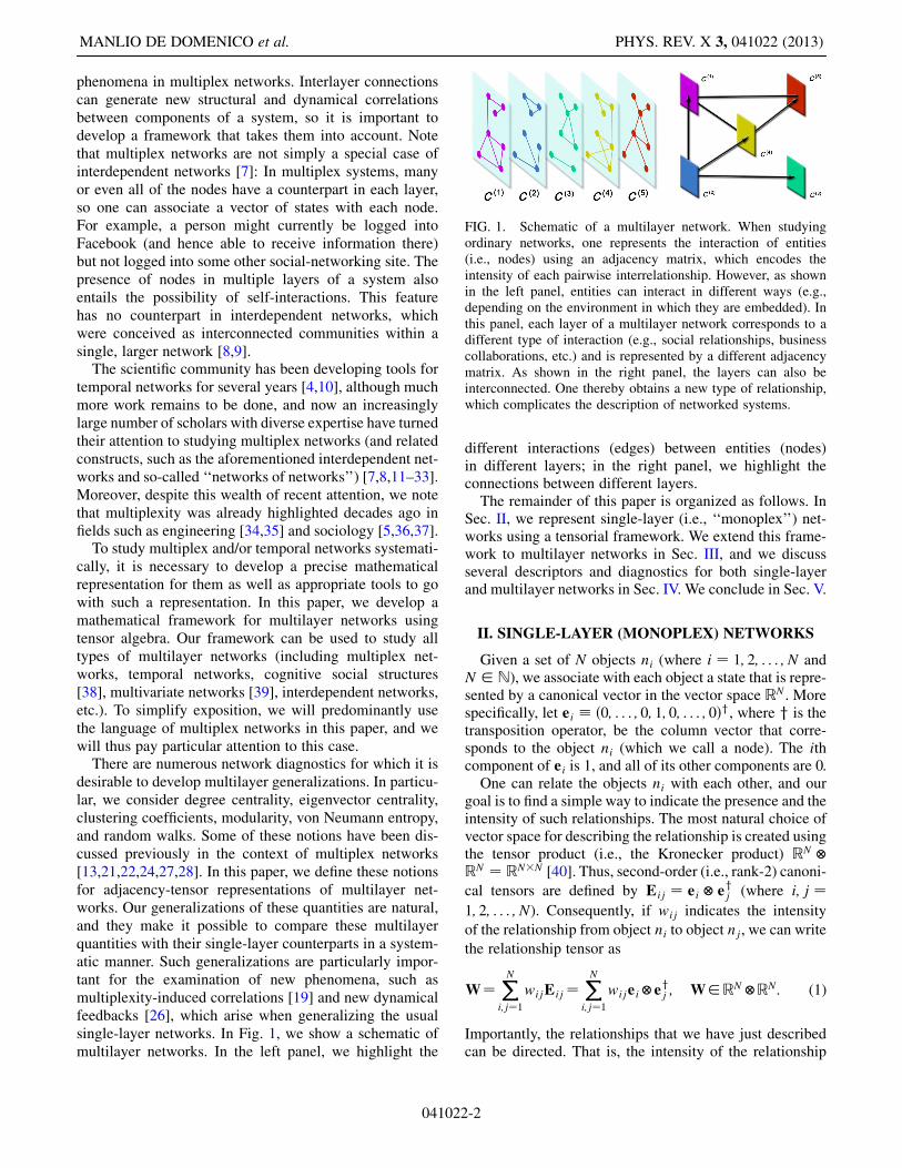
There are numerous network diagnostics for which it isdesirable to develop multilayer generalizations. In particu-lar, we consider degree centrality, eigenvector centrality,clustering coefficients, modularity, von Neumann entropy,and random walks. Some of these notions have been dis-cussed previously in the context of multiplex networks[13,21,22,24,27,28]. In this paper, we define these notionsfor adjacency-tensor representations of multilayer net-works. Our generalizations of these quantities are natural,and they make it possible to compare these multilayerquantities with their single-layer counterparts in a system-atic manner. Such generalizations are particularly impor-tant for the examination of new phenomena, such asmultiplexity-induced correlations [19] and new dynamicalfeedbacks [26], which arise when generalizing the usualsingle-layer networks. In Fig. 1, we show a schematic ofmultilayer networks. In the left panel, we highlight the

different interactions (edges) between entities (nodes)in different layers; in the right panel, we highlight theconnections between different layers.The remainder of this paper is organized as follows. In

Sec. II, we represent single-layer (i.e., ‘‘monoplex’’) net-works using a tensorial framework. We extend this frame-work to multilayer networks in Sec. III, and we discussseveral descriptors and diagnostics for both single-layerand multilayer networks in Sec. IV. We conclude in Sec. V.

II. SINGLE-LAYER (MONOPLEX) NETWORKS

Given a set of N objects ni (where i ¼ 1; 2; . . . ; N andN 2 N), we associate with each object a state that is repre-sented by a canonical vector in the vector space RN . Morespecifically, let ei � ð0; . . . ; 0; 1; 0; . . . ; 0Þy, where y is thetransposition operator, be the column vector that corre-sponds to the object ni (which we call a node). The ithcomponent of ei is 1, and all of its other components are 0.One can relate the objects ni with each other, and our

goal is to find a simple way to indicate the presence and theintensity of such relationships. The most natural choice ofvector space for describing the relationship is created usingthe tensor product (i.e., the Kronecker product) RN �RN ¼ RN�N [40]. Thus, second-order (i.e., rank-2) canoni-

cal tensors are defined by Eij ¼ ei � eyj (where i; j ¼1; 2; . . . ; N). Consequently, if wij indicates the intensity

of the relationship from object ni to object nj, we can write

the relationship tensor as

W¼ XNi;j¼1

wijEij¼XNi;j¼1

wijei�eyj ; W2RN�RN: (1)

Importantly, the relationships that we have just describedcan be directed. That is, the intensity of the relationship

FIG. 1. Schematic of a multilayer network. When studyingordinary networks, one represents the interaction of entities(i.e., nodes) using an adjacency matrix, which encodes theintensity of each pairwise interrelationship. However, as shownin the left panel, entities can interact in different ways (e.g.,depending on the environment in which they are embedded). Inthis panel, each layer of a multilayer network corresponds to adifferent type of interaction (e.g., social relationships, businesscollaborations, etc.) and is represented by a different adjacencymatrix. As shown in the right panel, the layers can also beinterconnected. One thereby obtains a new type of relationship,which complicates the description of networked systems.

MANLIO DE DOMENICO et al. PHYS. REV. X 3, 041022 (2013)

041022-2

from object ni to object nj need not be the same as the

intensity of the relationship from object nj to object ni.

In the context of networks, W corresponds to an N � Nweight matrix that represents the standard graph of asystem that consists of N nodes ni. This matrix is thus anexample of an adjacency tensor, which is the language thatwe will use in the rest of this paper. To distinguish suchsimple networks from the more complicated situations(e.g., multiplex networks) that we discuss in this paper,we will use the term monoplex networks to describe suchstandard networks, which are time independent and pos-sess only a single type of edge that connects their nodes.

Tensors provide a convenient mathematical representa-tion for generalizing ordinary static networks, as theyprovide a natural way to encapsulate complicated sets ofrelationships that can also change in time [13,41]. Matricesare rank-2 tensors, so they are inherently limited in thecomplexity of the relationships that they can capture. Onecan represent increasingly complicated types of relation-ships between nodes by considering tensors of higherorder. An adjacency tensor can be written using a morecompact notation that will be useful for the generalizationto multilayer networks that we will discuss later. We willuse the covariant notation introduced by Ricci and Levi-Civita in Ref. [42]. In this notation, a row vector a 2 RN isgiven by a covariant vector a� (where � ¼ 1; 2; . . . ; N),and the corresponding contravariant vector a� (i.e., its dualvector) is a column vector in Euclidean space.

To avoid confusion, we will use latin letters i; j; . . . toindicate, for example, the ith vector, the ðijÞth tensor, etc.,and we will use greek letters �;�; . . . to indicate thecomponents of a vector or a tensor. With this terminology,e�ðiÞ is the �th component of the ith contravariant canoni-cal vector ei in RN , and e�ðjÞ is the �th component of thejth covariant canonical vector in RN .

With these conventions, the adjacency tensor W canbe represented as a linear combination of tensors in thecanonical basis:

W�� ¼ XN

i;j¼1

wije�ðiÞe�ðjÞ ¼

XNi;j¼1

wijE��ðijÞ; (2)

where E��ðijÞ 2 RN�N indicates the tensor in the canonical

basis that corresponds to the tensor product of the canoni-cal vectors assigned to nodes ni and nj (i.e., it is Eij).

The adjacency tensor W�� is of mixed type: it is

1-covariant and 1-contravariant. This choice provides anelegant formulation for the subsequent definitions.

III. MULTILAYER NETWORKS

In the previous section, we described a procedure tobuild an adjacency tensor for a monoplex (i.e., single-layer) network. In general, however, there might be severaltypes of relationships between pairs of nodes n1;n2; . . . ; nN , and an adjacency tensor can be used to

represent this situation. In other words, one can think ofa more general system represented as a multilayer object inwhich each type of relationship is encompassed in a single

layer ~k (where ~k ¼ 1; 2; . . . ; L) of a system.We use the term intralayer adjacency tensor for the

second-order tensor W��ð~kÞ that indicates the relationships

between nodes within the same layer ~k. The tilde symbolallows us to distinguish indices that correspond to nodesfrom those that correspond to layers.We take into account the possibility that a node ni from

layer ~h can be connected to any other node nj in any other

layer ~k. To encode information about relationships thatincorporate multiple layers, we introduce the second-order

interlayer adjacency tensor C��ð~h ~kÞ. Note that C�

�ð~k ~kÞ ¼W�

�ð~kÞ, so the interlayer adjacency tensor that corresponds

to the case in which a pair of layers represents the same

layer ~k is equivalent to the intralayer adjacency tensor ofsuch a layer.Following an approach similar to that in Sec. II, we

introduce the vectors e~�ð~kÞ (where ~� ¼ 1; 2; . . . ; L and~k ¼ 1; 2; . . . ; L) of the canonical basis in the space RL,where the greek index indicates the components of thevector and the latin index indicates the kth canonicalvector. The tilde symbol on the greek indices allows usto distinguish these indices from the greek indices thatcorrespond to nodes. It is straightforward to construct the

second-order tensors E~�~�ð~h ~kÞ ¼ e~�ð~hÞe~�ð~kÞ that represent

the canonical basis of the space RL�L. (We use analogousnotation for canonical bases throughout this paper.)We can write the multilayer adjacency tensor discussed

early in this section using a tensor product between the

adjacency tensors C��ð~h ~kÞ and the canonical tensors

E~�~�ð~h ~kÞ. We obtain

M�~�

� ~�¼ XL

~h;~k¼1

C��ð~h ~kÞE~�

~�ð~h ~kÞ

¼ XL~h;~k¼1

24 XN

i;j¼1

wijð~h ~kÞE��ðijÞ

35E~�

~�ð~h ~kÞ

¼ XL~h;~k¼1

XNi;j¼1

wijð~h ~kÞE�~�

� ~�ðij~h ~kÞ; (3)

where wijð~h ~kÞ are real numbers that indicate the intensity

of the relationship (which may not be symmetric) between

nodes ni in layer ~h and node nj in layer ~k, and E�~�

� ~�ðij~h ~kÞ �

e�ðiÞe�ðjÞe~�ð~hÞe~�ð~kÞ indicates the fourth-order (i.e., rank-4) tensors of the canonical basis in the space RN�N�L�L.

The multilayer adjacency tensor M�~�

� ~�is a very general

object that can be used to represent a wealth of complicatedrelationships among nodes. In this paper, we focus onmultiplex networks. A multiplex network is a special

MATHEMATICAL FORMULATION OF MULTILAYER NETWORKS PHYS. REV. X 3, 041022 (2013)

041022-3

type of multilayer network in which the only possible typesof interlayer connections are ones in which a given node isconnected to its counterpart nodes in the other layers. Inmany studies of multiplex networks, it is assumed (at leastimplicitly) that interlayer connections exist between coun-terpart nodes in all pairs of layers. However, (i) this as-sumption need not hold, and (ii) it departs from traditionalnotions of multiplexity [5], which focus on the existence ofmultiple types of connections and do not preclude entitiesfrom possessing only a subset of the available categories ofconnections. We thus advocate a somewhat more general(and more traditional) definition of multiplex networks.

When describing a multiplex network, the associatedinterlayer adjacency tensor is diagonal. Importantly, con-nections between a node and its counterparts can havedifferent weights for different pairs of layers, and inter-layer connections can also be different for different en-tities in a network [43]. For instance, such considerationsare important for transportation networks, where one canrelate the weight of interlayer connections to the costof switching between a pair of transportation modes(i.e., layers). For example, at a given station (i.e., node)in a transportation network, it takes time to walk from atrain platform to a bus, and it is crucial for transporta-tion companies to measure how long it takes to changetransportation modes [44]. See Fig. 2 for schematics ofmultiplex networks.

As we discussed above, entities in many systems haveconnections in some layers but not in others. For example,a user of online social networks might have a Facebookaccount but not use Twitter. Such an individual can thusbroadcast and receive information only on a subset of thelayers in the multiplex-network representation of the sys-tem. In a transportation network, if a station does not existin a given layer of a multilayer network, then its associatededges also do not exist. The algebra in this paper holdsfor these situations without any formal modification(one simply assigns the value 0 to associated edges),but one must think carefully about the interpretation ofcalculations of network diagnostics.

If there is only a single layer, there is no distinctionbetween a monoplex network and a single-layer network,so we can use these terms interchangeably. However, thedifference is crucial when studying multilayer networks.Importantly—because it is convenient, for instance, for theimplementation of computational algorithms—one can

represent the multilayer adjacency tensorM�~�

� ~�as a special

rank-2 tensor that one obtains by a process called matrici-zation (which is also known as unfolding and flattening)

[45]. The elements of M�~�

� ~�, which is defined in the space

RN�N�L�L, can be represented as an N2 � L2 or anNL� NLmatrix. Flattening a multilayer adjacency tensorcan be very helpful. Recent studies on communitydetection [13,46], diffusion [21], random walks [22],social contagions [27,28], and clustering coefficients [47]on multilayer networks have all used matrix representationsof multilayer networks for computational (and occasionallyanalytical) purposes. For many years, the computational-science community has stressed the importance of devel-oping tools for both tensors and their associated unfoldings(see the review article [45] and numerous referencestherein) and of examining problems from these comple-mentary perspectives. We hope that this paper will helpfoster similar achievements in network science.Another important special case of multilayer adjacency

tensors is time-dependent (i.e., ‘‘temporal’’) networks.Multilayer representations of temporal networks havethus far tended to include only connections between agiven node in one layer and its corresponding nodes inits one or two neighboring layers. For example, thenumerical calculations in Refs. [13,41] only use these‘‘ordinal’’ interlayer couplings, which causes the off-diagonal blocks of a flattened adjacency tensor to havenonzero entries only along their diagonals, even though thetheoretical formulation in those papers allows more gen-eral couplings between layers. Indeed, this restriction doesnot apply, in general, to temporal networks, as it is impor-tant for some applications to consider more general typesof interlayer couplings (e.g., if one is considering causal

FIG. 2. Schematic of multilayer networks for three different topologies. We show three four-layer multiplex networks (and thecorresponding network of layers as an inset in the top-left corners) and recall that each interlayer edge connects a node with one of itscounterparts in another layer.

MANLIO DE DOMENICO et al. PHYS. REV. X 3, 041022 (2013)

041022-4

relationships between different nodes or if one wants toconsider interlayer coupling over a longer time horizon).In temporal networks that are constructed from coupledtime series, the individual layers in a multilayer adjacencytensor tend to be almost completely connected (althoughthe intralayer edges, of course, have different weights).In other cases, such as most of the temporal networksdiscussed in Ref. [4], there might only be a small numberof nonzero connections (which represent, e.g., a smallnumber of phone calls in a particular time window) withina single layer.

IV. NETWORK DESCRIPTORS ANDDYNAMICAL PROCESSES

In this section, we examine how to generalize some ofthe most common network descriptors and dynamical pro-cesses for multilayer networks. First, we use our tensorialconstruction to show that the properties of a multilayernetwork when it is made up of only a single layer reduce tothe corresponding ones for a monoplex network. We obtainthese properties using algebraic operations involvingthe adjacency tensor, canonical vectors, and canonicaltensors. We then generalize these results for more generalmultilayer adjacency tensors.

A. Monoplex networks

Degree centrality.—Consider an undirected andunweighted network, which can be represented usingthe (symmetric) adjacency tensor W�

� . Define the 1-vector

u� ¼ ð1; . . . ; 1Þy 2 RN whose components are all equal

to 1, and let U�� ¼ u�u

� be the second-order tensorwhose elements are all equal to 1. (Throughout this paper,we use analogous notation for all so-called ‘‘1-tensors,’’whose entries are all equal to 1.) We adopt Einsteinsummation notation (see Appendix A) and interpretthe adjacency tensor as an operator to be applied to the1-vector.

We thereby calculate the degree centrality vector(or degree vector) k� ¼ W�

�u� in the space RN . It is then

straightforward to calculate the degree centrality of node niby projecting the degree vector onto the ith canonicalvector: kðiÞ ¼ k�e

�ðiÞ. Analogously, for an undirected

and weighted network, we use the corresponding weightedadjacency tensor W�

� to define the strength centrality vec-

tor (or strength vector) s�, which can be used to calculate

the strength (i.e., weighted degree) [48,49] of each node.With our notation, the mean degree is hki ¼ ðU�

�Þ�1k�u�,

the second moment of the degree is hk2i ¼ ðU��Þ�1k�k

�,

and the variance of the degree is varðkÞ ¼ ðU��Þ�1k�k

� �ðU�

��2k�k�U��.

Directed networks are also very important, and theyillustrate why it is advantageous to introduce contravariantnotation. Importantly, in-degree centrality and out-degreecentrality are represented using different tensor products.

The in-degree centrality vector is k� ¼ W��u�, whereas the

out-degree centrality vector is k� ¼ W��u

�. We then re-

cover the usual definitions for directed networks. Forexample, the in-degree centrality of node ni is kinðiÞ ¼W�

�u�e�ðiÞ. In directed and weighted networks, the analo-

gous definition yields the in-strength centrality vector andthe out-strength centrality vector. These calculations withdirected networks are simple, but they illustrate that theproposed tensor algebra makes it possible to develop adeeper understanding of networks, as the tensor indicesare related directly to the directionality of relationshipsbetween nodes in a network.Clustering coefficients.—Clustering coefficients are

useful measures of transitivity in a network [50]. Forunweighted and undirected networks, the local clusteringcoefficient of a node ni is defined as the number of existingedges among the set of its neighboring nodes divided bythe total number of possible connections between them[51]. Several different definitions for local clusteringcoefficients have been developed for weighted and undir-ected networks [49,52–54] and for directed networks [55].Given a local clustering coefficient, one can calculate adifferent global clustering coefficient by averaging over allnodes. Alternatively, one can calculate a global clusteringcoefficient as the total number of closed triples of nodes(where all three edges are present) divided by the numberof connected triples [2].One can obtain equivalent definitions of clustering

coefficients in terms of walks on a network. In standardnetwork theory, suppose that one has an adjacency matrixA and a positive integer m. Then, each matrix elementðAmÞij gives the number of distinct walks of length m that

start from node ni and end at node nj. Therefore, taking

j ¼ i andm ¼ 3 yields the number of walks of length threethat start and end at node ni. In an unweighted networkwithout self-loops, we thereby obtain the number ofdistinct three-cycles tðiÞ that start from node ni. One thencalculates the local clustering coefficient of node ni bydividing tðiÞ by the number of three-cycles that would existif the neighborhood of ni were completely connected. Forexample, in an undirected network, one divides tðiÞ by kðiÞ[kðiÞ � 1], which is the number of ways to select two of theneighbors of ni. In our notation, the value of ðAmÞij is

tði; jÞ ¼ W��1W�1

�2W�2

�3� � �W�m�2

�m�1W�m�1

� e�ðiÞe�ðjÞ; (4)

which reduces to tðiÞ ¼ W��W

��W�

�e�ðiÞe�ðiÞ for j ¼ i and

m ¼ 3. One can then define the local clustering coefficientby dividing the number of three-cycles by the number ofthree-cycles in a network for which the neighborhood ofthe node ni is completely connected. We thereby obtain theformula

cðW��; iÞ ¼

W��W

��W�

�e�ðiÞe�ðiÞW�

�F��W�

�e�ðiÞe�ðiÞ; (5)

MATHEMATICAL FORMULATION OF MULTILAYER NETWORKS PHYS. REV. X 3, 041022 (2013)

041022-5

where

F�� ¼ U

�� � �

��

is the adjacency tensor corresponding to a network thatincludes all edges except for self-loops.

To use the above formulation to calculate a globalclustering coefficient of a network, we need to calculateboth the total number of three-cycles and the total numberof three-cycles that one obtains when the second step of thewalk occurs in a complete network. A compact way toexpress this global clustering coefficient is

cðW��Þ ¼

W��W

��W�

�

W��F

��W�

�

: (6)

One can define a clustering coefficient in a weighted net-work without any changes to Eqs. (5) and (6) by assumingthat W�

� corresponds to the weighted adjacency tensor

normalized such that each element of the tensor lies inthe interval [0, 1]. If weights are not defined within thisrange, then Eqs. (5) and (6) do need to be modified. Onemight also wish to modify Eq. (5) to explore generaliza-tions of the several existing weighted clustering coeffi-cients for ordinary networks [52].

We now modify Eq. (6) to consider weighted clusteringcoefficients more generally. Let N be a real number thatcan be used to rescale the elements of the tensor. Define~W�� ¼ W�

�=N , where one can define the normalization

N in various ways. For example, it can come from themaximum (so that N ¼ max�;�fW�

�g). It is straightfor-

ward to show that cð ~W��Þ ¼ cðW�

�Þ=N . Therefore, we

redefine the global clustering coefficient cðW��Þ from

Eq. (5) using this normalization:

cðW��Þ ¼ N �1

W��W

��W�

�

W��F

��W�

�

: (7)

The same argument applies in the case of the localclustering coefficient for weighted networks. The choiceof the norm in the normalization factor N is an importantconsideration. For example, the choiceN ¼ max�;�fW�

�gensures that Eq. (7) reduces to Eq. (6) for unweightednetworks.

Eigenvector and Katz centralities.—Numerous notionsof centrality exist to attempt to quantify the importance ofnodes (and other components) in a network [5]. For ex-ample, a node ni has a high eigenvector centrality if itsneighbors also have high eigenvector centrality, and therecursive nature of this notion yields a vector of centralitiesthat satisfies an eigenvalue problem.

Let A be the adjacency matrix for an undirected net-work, v be a solution of the equation Av ¼ �1v, and �1

be the largest (‘‘leading’’) eigenvalue of A. Thus, v isthe leading eigenvector of A, and the components of vgive the eigenvector centralities of the nodes. That is, theeigenvector centrality of node ni is given by vi [56,57].

In our tensorial formulation, the eigenvector centralityvector is a solution of the tensorial equation

W��v� ¼ �1v�; (8)

and v�e�ðiÞ gives the eigenvector centrality of node ni.

For directed networks, there are two leading eigenvec-tors, and one needs to take into account the differencebetween Eq. (8) and its contravariant counterpart.Moreover, nodes with only outgoing edges have an eigen-vector centrality of 0 if the above definition is adopted. Oneway to address this situation is to assign a small amount bof centrality to each node before calculating centrality. Oneincorporates this modification of eigenvector centrality byfinding the leading-eigenvector solution of the eigenvalueproblem v ¼ aAvþ b1, where 1 is a vector in which eachentry is a 1. This type of centrality is known as Katzcentrality [58]. One often chooses b ¼ 1, and we notethat Katz centrality is well defined if ��1

1 > a. Usingtensorial notation, we obtain

v� ¼ ð��� � aW�

�Þ�1u�: (9)

To calculate Katz centrality from Eq. (9), we need tocalculate the tensor inverse T�

� , which satisfies the equation

T��ð��

� � aW�� Þ ¼ ��

�.

Modularity.—It is often useful to decompose networksinto disjoint sets (‘‘communities’’) of nodes such that(relative to some null model) nodes within each commun-ity are densely connected to each other but connectionsbetween communities are sparse. Modularity is a networkdescriptor that can be calculated for any partition of anetwork into disjoint sets of nodes. Additionally, one canattempt to algorithmically determine a partition that max-imizes modularity to identify dense communities in amonoplex network. There are many ways to maximizemodularity as well as many other ways to algorithmicallydetect communities (see the review articles [59,60]). Wewill consider Newman-Girvan modularity [61], which isthe most popular version of modularity and can be writtenconveniently in matrix notation [62,63]. Let S�a be a tensorin RN�M, where � indexes nodes and a indexes the com-munities1 in an undirected network, which can be eitherweighted or unweighted. The value of a component of S�a isdefined to be 1 when a node belongs to a particular com-munity and 0 when it does not. We introduce the tensor

B�� ¼ W�

� � k�k�=K, whereK ¼ W��U

�� . It follows that

the modularity of a network partition is given by the scalar2

Q ¼ 1

KSa�B

��S

�a : (10)

1The reader should be careful to not confuse the latter latinindex with the indices that we have used thus far.

2Recall that swapping subscripts and superscripts (and hencecovariance and contravariance) in a tensor is an implicit use of atransposition operator [40].

MANLIO DE DOMENICO et al. PHYS. REV. X 3, 041022 (2013)

041022-6

To consider a general null model, we write B�� ¼

W�� � P�

�, where P�� is a tensor that encodes the random

connections against which one compares a network’s ac-tual connections. With this general null-model tensor,modularity is also appropriate for directed networks(although, of course, it is still necessary to choose anappropriate null model).

von Neumann entropy.—The study of entropy in mono-plex networks has been used to help characterize complex-ity in networked systems [64–68]. As an example, let usconsider the von Neumann entropy of a monoplex network[69]. Recall that the von Neumann entropy extends theShannon (information) entropy to quantum systems. Inquantum mechanics, the density matrix � is a positivesemidefinite operator that describes the mixed state of aquantum system, and the von Neumann entropy of � isdefined by H ð�Þ ¼ �trð�log2�Þ. The eigenvaluesof � must sum to 1 to have a well-defined measure ofentropy.

We also need to recall the (unnormalized) combinatorialLaplacian tensor, which is a well-known object in graphtheory (see, e.g., Refs. [70,71] and references therein)and is defined by L�

� ¼ ��� �W�

� , where ��� ¼

W�ue

�ð�Þ��� is the strength tensor (i.e., a diagonal tensor

whose elements represent the strength of the nodes). Thecombinatorial Laplacian is positive semidefinite, and thetrace of the strength tensor is � ¼ ��

�. The eigenvalues ofthe density tensor ��

� ¼ ��1L�� sum to 1, as required, and

they can be used to define the von Neumann entropy of amonoplex network using the formula

H ðW��Þ ¼ ���

�log2½����: (11)

Using the eigendecomposition of the density tensor, onecan show that the von Neumann entropy reduces to

H ðW��Þ ¼ ���

�log2½����; (12)

where ��� is the diagonal tensor whose elements are the

eigenvalues of ��� (see Appendix C).

Diffusion and random walks.—A random walk is thesimplest dynamical process that can occur on a monoplexnetwork, and random walks can be used to approximateother types of diffusion [2,72]. Diffusion is also relevantfor many other types of dynamical processes (e.g., forsome types of synchronization [73]).

Let x�ðtÞ denote a state vector of nodes at time t. Thediffusion equation is

dx�ðtÞdt

¼ D½W��x�ðtÞ �W�

�u�e�ð�Þx�ðtÞ�; (13)

where D is a diffusion constant. Recall that s� ¼ W��u� is

the strength vector and that s�e�ð�Þx�ðtÞ ¼ s�e

�ð�Þ����x�ðtÞ. We obtain the following covariant diffusion law

on monoplex networks:

dx�ðtÞdt

¼ �DL��x�ðtÞ; (14)

where L�� ¼ W

�ue�ð�Þ��

� �W�� is the combinatorial

Laplacian tensor. The solution of Eq. (14) is x�ðtÞ ¼x�ð0Þe�DL�

�t.

Random walks on monoplex networks [2,72,74] haveattracted considerable interest because they are both im-portant and easy to interpret. They have yielded importantinsights on a huge variety of applications and can bestudied analytically. For example, random walks havebeen used to rank Web pages [75] and sports teams [76],optimize searches [77], investigate the efficiency of net-work navigation [78,79], characterize cyclic structures innetworks [80], and coarse grain networks to illuminatemesoscale features such as community structure [81–83].In this paper, we consider a discrete-time random walk.

Let T�� denote the tensor of transition probabilities between

pairs of nodes, and let p�ðtÞ denote the vector of proba-bilities to find a walker at each node. Hence, the covariantmaster equation that governs the discrete-time evolution ofthe probability from time t to time tþ 1 is p�ðtþ 1Þ ¼T��p�ðtÞ. One can rewrite this master equation in terms of

evolving probability rates as _p�ðtÞ ¼ � �L��p�ðtÞ, where

�L�� ¼ ��

� � T�� is the normalized Laplacian tensor. The

normalized Laplacian governs the evolution of theprobability-rate vector for random walks.

B. Multilayer networks

Because of its structure, a multilayer network can incor-porate a lot of information. Before generalizing the de-scriptors that we discussed for monoplex networks, wediscuss some algebraic operations that can be employedto extract useful information from an adjacency tensor.Contraction.—Tensor contractions yield interesting

quantities that are invariants when the indices are repeated(see Appendix A). For instance, one can obtain the numberof nodes in a network (which is an invariant quantity)by contracting the Kronecker tensor N ¼ ��

�, where wehave again used Einstein summation convention. Forunweighted networks, one obtains the number of edges(which is another invariant) by calculating the scalarproduct between the adjacency tensor W�

� with the dual

1-tensor U�� (whose components are all equal to 1).

Single-layer extraction.—In some applications, it can beuseful to extract a specific layer (e.g., the ~rth one) from amultilayer network. Using tensorial algebra, this operation

is equivalent to projecting the tensor M�~�

� ~�to the canonical

tensor E~�~�ð~r ~rÞ that corresponds to this particular layer.

The second-order canonical tensors in RL�L form an or-

thonormal basis, so the product E~�~�ð~h ~kÞE~�

~�ð~r ~rÞ equals 1 for~h ¼ ~k ¼ ~r and it equals 0 otherwise. Therefore, we useEq. (3) to write

MATHEMATICAL FORMULATION OF MULTILAYER NETWORKS PHYS. REV. X 3, 041022 (2013)

041022-7

M�~�

� ~�E

~�~�ð~r ~rÞ ¼ C�

�ð~r ~rÞ ¼ W��ð~rÞ; (15)

which is the desired adjacency tensor that corresponds tolayer ~r. Clearly, it is possible to use an analogous procedureto extract any other tensor (e.g., ones that give interlayerrelationships). In practical applications, for example, itmight be useful to extract the tensors that describe interlayerconnections between pairs of layers in the multilayer net-work to compare the strengths of the couplings betweenthem. Another important application, which we discusslater, is the calculation of multilayer clustering coefficients.

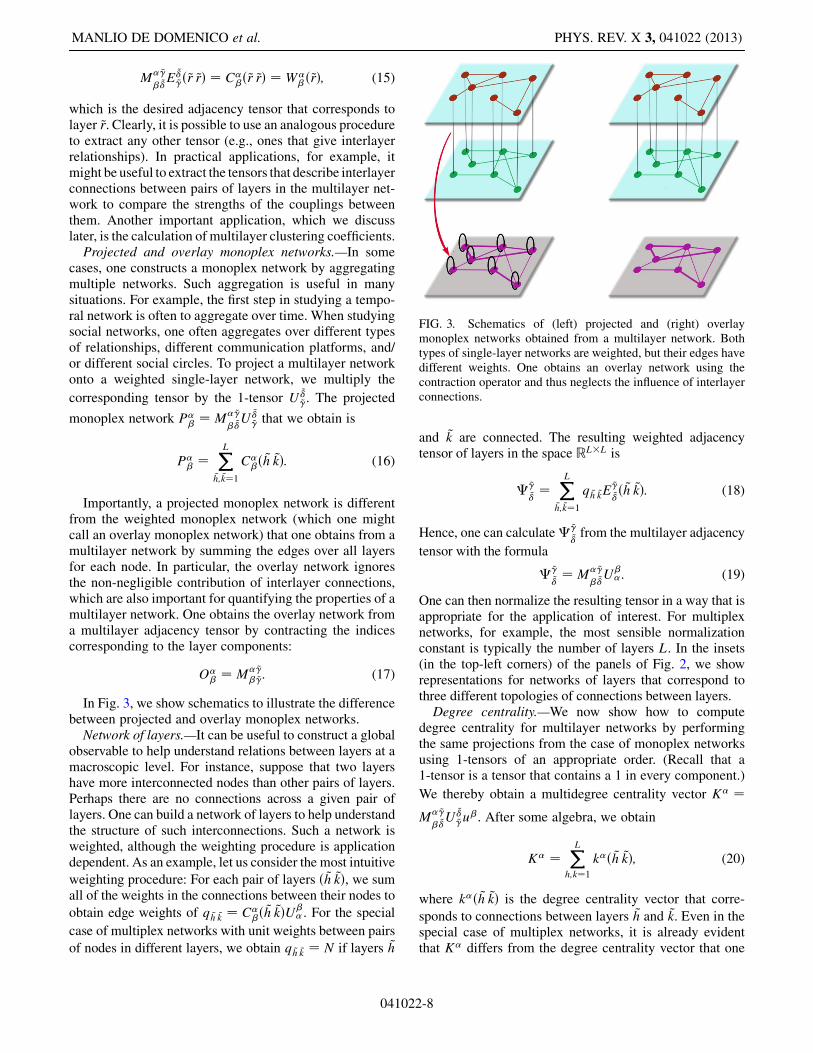
Projected and overlay monoplex networks.—In somecases, one constructs a monoplex network by aggregatingmultiple networks. Such aggregation is useful in manysituations. For example, the first step in studying a tempo-ral network is often to aggregate over time. When studyingsocial networks, one often aggregates over different typesof relationships, different communication platforms, and/or different social circles. To project a multilayer networkonto a weighted single-layer network, we multiply the

corresponding tensor by the 1-tensor U~�~�. The projected

monoplex network P�� ¼ M�~�

� ~�U

~�~� that we obtain is

P�� ¼ XL

~h;~k¼1

C��ð~h ~kÞ: (16)

Importantly, a projected monoplex network is differentfrom the weighted monoplex network (which one mightcall an overlay monoplex network) that one obtains from amultilayer network by summing the edges over all layersfor each node. In particular, the overlay network ignoresthe non-negligible contribution of interlayer connections,which are also important for quantifying the properties of amultilayer network. One obtains the overlay network froma multilayer adjacency tensor by contracting the indicescorresponding to the layer components:

O�� ¼ M�~�

�~�: (17)

In Fig. 3, we show schematics to illustrate the differencebetween projected and overlay monoplex networks.

Network of layers.—It can be useful to construct a globalobservable to help understand relations between layers at amacroscopic level. For instance, suppose that two layershave more interconnected nodes than other pairs of layers.Perhaps there are no connections across a given pair oflayers. One can build a network of layers to help understandthe structure of such interconnections. Such a network isweighted, although the weighting procedure is applicationdependent. As an example, let us consider the most intuitive

weighting procedure: For each pair of layers ð~h ~kÞ, we sumall of the weights in the connections between their nodes to

obtain edge weights of q~h ~k ¼ C��ð~h ~kÞU�

� . For the special

case of multiplex networks with unit weights between pairs

of nodes in different layers, we obtain q~h ~k ¼ N if layers ~h

and ~k are connected. The resulting weighted adjacencytensor of layers in the space RL�L is

�~�~�¼ XL

~h;~k¼1

q~h ~kE~�~�ð~h ~kÞ: (18)

Hence, one can calculate�~�~�from the multilayer adjacency

tensor with the formula

�~�~�¼ M�~�

�~�U�

�: (19)

One can then normalize the resulting tensor in a way that isappropriate for the application of interest. For multiplexnetworks, for example, the most sensible normalizationconstant is typically the number of layers L. In the insets(in the top-left corners) of the panels of Fig. 2, we showrepresentations for networks of layers that correspond tothree different topologies of connections between layers.Degree centrality.—We now show how to compute

degree centrality for multilayer networks by performingthe same projections from the case of monoplex networksusing 1-tensors of an appropriate order. (Recall that a1-tensor is a tensor that contains a 1 in every component.)

We thereby obtain a multidegree centrality vector K� ¼M�~�

� ~�U

~�~�u

�. After some algebra, we obtain

K� ¼ XLh;k¼1

k�ð~h ~kÞ; (20)

where k�ð~h ~kÞ is the degree centrality vector that corre-

sponds to connections between layers ~h and ~k. Even in thespecial case of multiplex networks, it is already evidentthat K� differs from the degree centrality vector that one

FIG. 3. Schematics of (left) projected and (right) overlaymonoplex networks obtained from a multilayer network. Bothtypes of single-layer networks are weighted, but their edges havedifferent weights. One obtains an overlay network using thecontraction operator and thus neglects the influence of interlayerconnections.

MANLIO DE DOMENICO et al. PHYS. REV. X 3, 041022 (2013)

041022-8

would obtain by simply projecting all layers of a multilayernetwork onto a single weighted network.

The definitions of mean degree, second moment, andvariance are analogous to the corresponding monoplex-network counterparts, except that one usesK� instead of k�.

Clustering coefficients.—For multilayer networks, it isnontrivial to define a clustering coefficient using trianglesas a measure of transitivity. As shown in Fig. 4, a closed setof three nodes might not exist on any single layer, buttransitivity can still arise as a consequence of multiplexity.In the left panel, for example, suppose that nodes A and Bare friends with node C but not with each other, but thatnodes A and B still have a social tie because they work atthe same company (but node C does not). In this situation,it is necessary for connections to exist on multiple layersfor it to be possible to transfer information from any onenode to any other node.

As with monoplex networks, we start by defining theinteger power of an adjacency tensor and use a contraction

operation. For instance, one can calculate the square ofM�~�

� ~�

by constructing the eighth-order (i.e., rank-8) tensor

M�~�

� ~�M�~

�~ and then contracting � with � and ~� with ~.

One computes higher powers analogously. We definea global clustering coefficient on a multilayer adjacencytensor by generalizing Eq. (6) for fourth-order tensors:

cðM�~�

� ~�Þ ¼ N �1

M�~�

� ~�M� ~�

~M~�~�

M�~�

� ~�F� ~�~M

~�~�

; (21)

where we again define F� ~�~ ¼ U� ~�

~ � �� ~�~ as the adjacency

tensor of a complete multilayer network (without self-edges). The choice of the normalization factor N is again

arbitrary, but the choiceN ¼ max�;�;~�; ~�fM�~�

� ~�g ensures that

Eq. (21) is well defined for both weighted and unweightedmultilayer networks.The tensor contractions in Eq. (21) count all of the three-

cycles, including ones in which a walk goes through anycombination of interlayer and intralayer connections. Thus,for multiplex networks with categorical layers, Eq. (21)counts not only fully intralayer three-cycles but also theinterlayer three-cycles that are induced by the connection ofnodes to their counterparts in all of the other layers.A more traditional, and also simpler, approach to

calculating a global clustering coefficient of a multilayernetwork is to project it onto a single weighted network[i.e., the overlay networkO�

� defined by Eq. (17)] and then

calculate a clustering coefficient for the resulting network.In this case, we obtain

cðO��Þ ¼ M�1

M�~��~�M

� ~�

~�M~

�~

M�~��~�F

� ~�

~�M

~�~

; (22)

where M ¼ max�;�fM�~��~�g=L. In the chosen normaliza-

tion, note that we need to include a factor for the numberof layers L because the construction of the overlay networkdiscards the information about the number of layers. Forexample, adding an empty layer to a multilayer networkdoes not affect the resulting overlay network, but it in-creases the number of possible walks that one must con-sider in Eq. (22). In general, the clustering coefficientin Eq. (22) is different from the one in Eq. (21) becauseEq. (22) discards all interlayer connections. However, thereare some special cases when Eq. (22) and Eq. (21) take thesame value. In particular, these equations yield the samevalue when there is only a single layer or, more generally,when there are no interlayer edges and all of the intralayernetworks are exactly the same.The global clustering coefficient defined in Eq. (22)

sums the contributions of three-cycles for which eachstep of a walk is on the same layer and those for which awalk traverses two or three layers. We decompose thisclustering coefficient to separately count the contributionsof three-cycles that take place on one, two, and three layers[47]. Using our tensorial framework, we modify Eq. (22) asfollows:

FIG. 4. Schematic of closing triangles in multiplex networks.Triangles can be closed using intralayer connections from differ-ent layers. In the figure, we show two different situations that canarise. For example, the left panel might represent a multilayersocial network in which nodes A and B are friends of node C butare not friends with each other (first layer), but nodes A and Bstill have a social tie because they work in the same companyeven though node C does not work there (third layer). In the rightpanel, one might imagine that each layer corresponds to adifferent online social network: Perhaps node B tweets aboutan item; node C sees node B’s post on Twitter (first layer) andthen posts the same item on Facebook (second layer); node Athen sees this post and blogs about it (third layer), and node Breads this blog entry.

MATHEMATICAL FORMULATION OF MULTILAYER NETWORKS PHYS. REV. X 3, 041022 (2013)

041022-9

cðM�~�

� ~�; w�Þ ¼

M�~�

�~�M�~�

�~�M�~�~

PL~h;~k;~l¼1

E~�~�ð~h ~hÞE~�

~� ð~k ~kÞE~~ð~l ~lÞ��ð~h; ~k; ~lÞw�

M�~�

� ~�F�~��~�M

�~�~

PL~h;~k;~l¼1

E~�~�ð~h ~hÞE ~�

~� ð~k ~kÞE~~ð~l ~lÞ��ð~h; ~k; ~lÞw�

; (23)

where we have employed layer extraction operations(see our earlier discussion), w� is a vector that weightsthe contribution of three-cycles that span� layers, and ��

(where � ¼ 1; 2; 3) is a function that selects the cycleswith � layers:

�1ð~h; ~k; ~lÞ ¼ �~h ~l�~h ~k�~k ~l;

�2ð~h; ~k; ~lÞ ¼ ð1� �~h ~lÞ�~h ~k þ ð1� �~k ~lÞ�~h ~k þ ð1� �~h ~kÞ�~k ~l;

�3ð~h; ~k; ~lÞ ¼ ð1� �~h ~lÞð1� �~k ~lÞð1� �~h ~kÞ:We recover Eq. (22) with the choicew� ¼ ð1=3; 1=3; 1=3Þ.[We note that cðM�~�

� ~�; w�Þ ¼ cðM�~�

� ~�; c0w

�Þ for anynonzero constant c0, although we still normalize w� byconvention.] By contrast, with the choice ofw� ¼ ð1; 0; 0Þ,we only consider three-cycles in which every step of a walkis on the same layer.

Importantly, we can define the weight vector w� in theclustering coefficient in Eq. (23) so that it takes into accountthat there might be some cost for crossing different layers.As discussed in Ref. [47], one determines this ‘‘cost’’ basedon the dynamics and the application of interest. For ex-ample, if one is studying a dynamical process whose timescale is very fast compared to the time scale (i.e., the cost)associated with changing layers, then it is desirable toconsider the contribution from only one layer (i.e., the onein which the dynamical process occurs). For other dynami-cal processes, it is compulsory to also include contributionsfrom two or three layers. To give a brief example, considertransportation at the King’s Cross/St. Pancras station inLondon. This station includes a node in a layer that de-scribes travel via London’s metropolitan transportation sys-tem, a node in a layer for train travel within England, and anode for international train travel. A relevant cost is thenrelated to how long it takes to travel between different partsof the station [44]. One needs to consider such intrastationtravel time in comparison to the schedule times of severaltransportation mechanisms. By contrast, there is typicallyvery little cost associated with a person seeing informationon Facebook and then posting it on Twitter.

In the above definition, the entries of F� ~�~ are all equal to

1 except for self-edges. Sometimes, we need to instead use

a tensor �F� ~�~ that we construct by setting some of the off-

diagonal entries of F� ~�~ to 0. If the original multilayer net-

work cannot have a particular edge, then the tensor �F� ~�~

needs to have a 0 in its corresponding entry. For example,we need to use such 0 entries for multilayer networks whosestructural constraints forbid the existence of some nodes incertain layers or forbid certain inter- and intralayer edges.It is also necessary for multiplex networks, for which

interlayer edges can only exist between nodes and theircounterparts in other layers. Note, however, that using the

tensor �F�~�~ instead of F� ~�

~ influences the normalization of

clustering coefficients, as it affects the set of potential three-cycles that can exist in a multilayer network.Eigenvector centrality.—Generalizing eigenvector cen-

trality for a multilayer network is not trivial, and there areseveral possible ways to do it [24].References [21,22,27,28] recently introduced the

concepts of supra-adjacency (i.e., ‘‘superadjacency’’) andsupra-Laplacian (i.e., super-Laplacian) matrices to formu-late and solve eigenvalue problems in multiplex networks.Such supramatrices correspond to unique unfoldings ofcorresponding fourth-order tensors to obtain square matri-ces. It is worth noting that the tensorial space in which themultilayer adjacency tensor exists is RN�N�L�L, and thereexists a unique unfolding—up to the L! permutations ofdiagonal blocks of size N � N in the resulting space—thatprovides a square supra-adjacency tensor defined inRNL�NL. We now exploit the same idea by arguing that asupraeigenvector corresponds to a rank-1 unfolding of asecond-order ‘‘eigentensor’’ V�~�. According to this unique

mapping, if �1 is the largest eigenvalue and V�~� is the

corresponding eigentensor, then it follows that

M�~�

� ~�V�~� ¼ �1V� ~�: (24)

Therefore, similarly to monoplex networks, one can cal-culate the leading eigentensor V�~� iteratively. Start with a

tensor X�~�ðt ¼ 0Þ, which we can take to be X�~�ðt ¼ 0Þ ¼U�~�. By writing X�~�ð0Þ as a linear combination of the

second-order eigentensors and by observing that X�~�ðtÞ ¼ðM�~�

� ~�ÞtX�~�ð0Þ, one can show that X�~�ðtÞ is proportional to

V�~� in the t ! 1 limit. The convergence of this approach

is ensured by the existence of the unfolding ofM, since theiterative procedure is equivalent to the one applied to thecorresponding supramatrices.We thereby obtain a multilayer generalization of

Bonacich’s eigenvector centrality [56,57]:

V� ~� ¼ ��11 M�~�

� ~�V�~�: (25)

The monoplex notion of eigencentrality grants impor-tance to a node based on its connection to other nodes. Oneneeds to be careful about both intralayer and interlayerconnections when interpreting the results of calculating amultilayer generalization of it. For example, the intralayerconnections in one layer might be more important thanthose in others. For interlayer connections, one might pon-der how much of a ‘‘bonus’’ an entity earns based on its

MANLIO DE DOMENICO et al. PHYS. REV. X 3, 041022 (2013)

041022-10

presence in multiple layers. (Contrast this situation with thecost that we discussed previously in the context of trans-portation networks.) For instance, many Web services at-tempt to measure the influence of people on social media bycombining information from multiple online social net-works, and one can choose which communication modes(i.e., layers) to include. Moreover, by considering an over-lay monoplex network or a projection monoplex network, itis possible to derive separate centrality scores for differentlayers. In the above example, an individual who possessesdifferent centrality scores in different network layers wouldreflect the different levels of importance that that person hason different social media.

Modularity.—A multilayer generalization of modularitywas derived in Ref. [13] by considering random walks on

networks. Let S�~�a be a tensor in RN�L�M, where ð�; ~�Þ

indexes nodes and a indexes the communities in an undir-ected multilayer network, which can be either weighted or

unweighted. The value of a component of S�~�a is defined

to be 1 when a node belongs to a particular community

and 0 when it does not. We introduce the tensor B�~��~� ¼

W�~��~� � P

�~�� ~�, where K ¼ W

�~��~�U

� ~��~� , and P

�~�� ~� is a null-

model tensor that encodes the random connections againstwhich one compares a multilayer network’s actual con-nections. It follows that the modularity of a partition of amultilayer network is given by the scalar

Q ¼ 1

KSa�~�B

�~��~�S

�~�a : (26)

There are numerous choices for the null-model tensor P�~��~�.

The null models discussed in Refs. [13,41,84] give specialcases of the multilayer modularity in Eq. (26).

von Neumann entropy.—To generalize the definition ofvon Neumann entropy to multilayer networks, we need togeneralize the definition of the Laplacian tensor. Such anextension is not trivial because one needs to considereigenvalues of a fourth-order tensor.

As we showed previously when generalizing eigenvec-tor centrality, the existence of a unique unfolding intosupramatrices allows one to define and solve the eigen-value problem

L�~�

�~�V�~� ¼ �V� ~�; (27)

where L�~�

�~�¼ ��~�

�~��M�~�

� ~�is the multilayer Laplacian ten-

sor, ��~�

� ~�¼ M~

�~�U~E�~�ð�~�Þ��~�

�~�is the multistrength ten-

sor (i.e., the rank-4 counterpart of the strength tensor ���

that we defined previously for monoplex networks), � is aneigenvalue, and V�~� is its corresponding eigentensor (i.e.,

the unfolded rank-1 supraeigenvector). We note that thereare at most NL different eigenvalues and correspondingeigentensors. (Additionally, note that the 1-tensor thatappears in the definition of the multistrength tensor hastwo subscripts and that the canonical-basis tensor has twosuperscripts.)

Let � ¼ ��~��~� be the trace of the multistrength

tensor. The eigenvalues of the multilayer density tensor

��~�

� ~�¼ ��1L�~�

�~�sum to 1, so we can use them to define the

von Neumann entropy of a multilayer network as

H ðMÞ ¼ ���~�

�~�log2½�� ~�

�~��; (28)

where ��~�

� ~�is the diagonal tensor whose elements are the

eigenvalues of ��~�

�~�.

Diffusion and random walks.—Diffusion in multiplexnetworks was investigated recently in Ref. [21]. A diffusionequation for multilayer networks needs to include termsthat account for interlayer diffusion. Let X�~�ðtÞ denote thestate tensor of nodes in each layer at time t. The simplestdiffusion equation for a multilayer network is then

dX�~�ðtÞdt

¼ M�~�

� ~�X�~�ðtÞ �M�~�

�~�U�~�E�~�ð� ~�ÞX�~�ðtÞ: (29)

As in the case of monoplex networks, we introduce themultilayer combinatorial Laplacian

L�~�

� ~�¼ M

~�~�U~E

�~�ð�~�Þ��~�

�~��M�~�

� ~�(30)

to obtain the following covariant diffusion equation formultilayer networks:

dX� ~�ðtÞdt

¼ �L�~�

� ~�X�~�ðtÞ: (31)

The solution of Eq. (31) isX� ~�ðtÞ ¼ X�~�ð0Þe�L�~�

�~�t, which is

a natural generalization of the result formonoplex networks.The study of random walks is important for many ap-

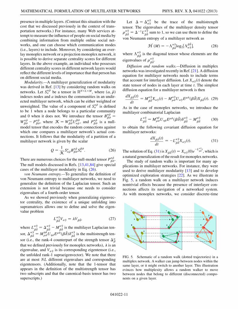
plications in multilayer networks. For instance, they wereused to derive multilayer modularity [13] and to developoptimized exploration strategies [22]. As we illustrate inFig. 5, a random walk on a multilayer network inducesnontrivial effects because the presence of interlayer con-nections affects its navigation of a networked system.As with monoplex networks, we consider discrete-time

FIG. 5. Schematic of a random walk (dotted trajectories) in amultiplex network. Awalker can jump between nodes within thesame layer, or it might switch to another layer. This illustrationevinces how multiplexity allows a random walker to movebetween nodes that belong to different (disconnected) compo-nents on a given layer.

MATHEMATICAL FORMULATION OF MULTILAYER NETWORKS PHYS. REV. X 3, 041022 (2013)

041022-11

random walks. Let T�~�

� ~�denote the tensor of transition

probabilities for jumping between pairs of nodes andswitching between pairs of layers, and let p�~�ðtÞ be the

time-dependent tensor that gives the probability to find awalker at a particular node in a particular layer. Hence, thecovariant master equation that governs the discrete-timeevolution of the probability from time t to time tþ 1 is

p�~�ðtþ 1Þ ¼ T�~�

�~�p�~�ðtÞ. We rewrite this master equation

in terms of evolving probability rates to obtain _p� ~�ðtÞ ¼� �L�~�

� ~�p�~�ðtÞ, where �L�~�

� ~�¼ ��~�

� ~�� T�~�

� ~�is the normalized

Laplacian tensor.

V. CONCLUSIONS AND DISCUSSION

In this paper, we developed a tensorial frameworkto study general multilayer networks. We discussed thegeneralization of several important network descriptors—including degree centrality, clustering coefficients, eigen-vector centrality, and modularity—for our multilayerframework. We examined different choices that one canmake in developing such generalizations, and we alsodemonstrated how our formalism yields results for mono-plex and multiplex networks as special cases.

As we have discussed in detail, our multilayer formalismprovides natural generalizations of network descriptors.Consequently, it allows systematic comparisons of multi-layer diagnostics with their single-layer counterparts. Aswe have also illustrated (e.g., for global clustering coef-ficients), our formalism also allows systematic compari-sons between different ways of generalizing familiarnetwork concepts. Such comparisons are particularly im-portant for the examination of new phenomena, such asmultiplexity-induced correlations [19], that arise whengeneralizing beyond the usual single-layer networks. Onecan obtain new insights even for simple descriptors like(directed) degree centrality, for which the tensor indices inour formulation are related directly to the directionality ofrelationships between nodes in a multilayer network.

The mathematical formalism that we have introducedcan be generalized further by considering higher-order(i.e., higher-rank) tensors. This generalization will providea systematic means to investigate networks that are, forexample, both time dependent and multiplex.

Our tensorial framework is an important step toward thedevelopment of a unified theoretical framework for study-ing networks with arbitrary complexities (including multi-plexity, time dependence, and more). When faced withgeneralizing the usual adjacency matrices to incorporatea feature such as multiplexity, different scholars haveemployed different notation and terminology, and it isthus desirable to construct a unified framework to unifythe language for studying networks. Moreover, in additionto defining mathematical notation that simplifies the han-dling and generalization of previously known diagnostics

on networks, a tensorial framework also offers the oppor-tunity to unravel new properties that remain hidden whenusing the classical approach of adjacency matrices. Wehope to construct a proper geometrical interpretation fortensorial representations of networks and to ultimatelyobtain an operational theory of dynamics both on and ofnetworks. This perspective has led to significant advancesin other areas of physics, and we believe that it will also beimportant for the study of networks.

ACKNOWLEDGMENTS

All authors were supported by the EuropeanCommission FET-Proactive Project PLEXMATH (GrantNo. 317614). A.A., M.D.D., S. G., and A. S. were alsosupported by the Generalitat de Catalunya 2009-SGR-838.A.A. also acknowledges financial support from the ICREAAcademia and the James S. McDonnell Foundation, andS.G. and A.A. were supported by FIS2012-38266. Y.M.was also supported by MINECO through GrantNo. FIS2011-25167 and by Comunidad de Aragon(Spain) through a grant to the group FENOL. M.A. P.acknowledges a grant (No. EP/J001759/1) from theEPSRC. We thank Peter Mucha and two anonymous ref-erees for useful comments.

APPENDIX A: EINSTEINSUMMATION CONVENTION

Einstein notation is a summation convention, which weadopt to reduce the notational complexity in our tensorialequations, that is applied to repeated indices in operationsthat involve tensors. For example, we use this conventionin the left-hand sides of the following equations:

A�� ¼ XN

�¼1

A��; A�B� ¼ XN

�¼1

A�B�;

A��B

�� ¼ XN

�¼1

A��B

��; A�

�B�� ¼ XN

�¼1

XN�¼1

A��B

��;

whose right-hand sides include the summation signs ex-plicitly. It is straightforward to use this convention for theproduct of any number of tensors of any order. Repeatedindices, such that one index is a subscript and the other is asuperscript, are equivalent to perform a tensorial operationknown as a contraction. Contracting indices reduces theorder of a tensor by 2. For instance, the contraction of thesecond-order tensor A�

� is the scalar A��, and the second-

order tensors A��B

�� and A�

�B�� are obtained by contracting

the fourth-order tensor A��B

��.

It is important to adopt Einstein summation on repeated

indices in a way that is unambiguous. For example, A�� ¼

A��, but A

��B

��C

�� is not equivalent to A�

�B��C

�� because of

the ambiguity about the index � in the second term of

A��B

��C

��. Specifically, it is not clear if the contraction B�

�

MANLIO DE DOMENICO et al. PHYS. REV. X 3, 041022 (2013)

041022-12

should be calculated before the product with the othertensors, or vice versa. Another situation that deservesparticular attention is equations that involve a ratio be-tween tensorial products, where one should separatelyapply the Einstein convention to the numerator and thedenominator. Thus, one should not perform products be-tween tensors B�

� and C�� with repeated indices � and � in

cases like

A��B

��

C��A

��

: (A1)

For example, see Eq. (5) in the main text.

APPENDIX B: DEFINITION OF THE TENSOREXPONENTIAL AND LOGARITHM

The exponential of a tensor B�� is a tensor A�

� such that

eB�� ¼ A�

�. The tensor exponential is defined by the power

series [85]

eB�� ¼ X1

m¼0

1

m!ðB�

�Þm; (B1)

where

ðB��Þm ¼ B�

�1B�1�2B�2�3� � �B�m�1

� : (B2)

A complete discussion of the properties of the tensorexponential is beyond the scope of the present paper.However, we show an example of how to calculate it fordiagonalizable tensors.

Let B�� be a diagonalizable tensor. In other words, there

exists a diagonal tensor D��, whose elements are the eigen-

values of B��, and a tensor J��, whose columns are the

eigenvectors of B��, such that B

��¼J��D

�� ðJ��Þ�1. It follows

that

ðB��Þm¼J��D

�� ðJ��1

Þ�1J�1�1D�1

�1 ðJ�1�2Þ�1 ���J�m�1

�m�1D�m�1

�m�1ðJ�m�1

� Þ�1¼J��ðD�

� ÞmðJ��Þ�1 (B3)

and

eB�� ¼ J��

�X1m¼0

1

m!ðD�

� Þm�ðJ��Þ�1 ¼ J��e

D�� ðJ��Þ�1: (B4)

The exponential of a diagonal tensor is the tensor obtainedby exponentiating each of the diagonal elementsD�

�, and it

is straightforward to calculate eD�� .

The logarithm of a tensor A�� is defined as the tensor B�

�

that satisfies the relation eB�� ¼ A�

�. It is straightforward to

show for a diagonal tensor A�� that

log½A��� ¼ J��½logD�

� �ðJ��Þ�1; (B5)

where D�� is the diagonal tensor whose elements are the

eigenvalues of A��, and J�� is a tensor whose columns are

the eigenvectors of A��.

APPENDIX C: DERIVATION OFVON NEUMANN ENTROPY

The von Neumann entropy of a monoplex networkis defined by Eq. (11). Let �� be the ith eigenvector(i ¼ 1; 2; . . . ; N) of the density tensor ��

�, and let ��� be

the tensor of eigenvectors. The density tensor is defined byrescaling the combinatorial Laplacian, so it has positivediagonal entries and nonpositive off-diagonal entries. It ispositive semidefinite and has non-negative eigenvalues.We diagonalize the density tensor to obtain ��

� ¼��

���� ð��

��1, where ��� is a diagonal tensor whose ele-

ments are the eigenvalues of ���. These eigenvalues are

equal to the eigenvalues of the combinatorial Laplaciantensor rescaled by the scalar ��1, where � ¼ ��

� and ���

is the strength tensor. It follows that

��� log2½��

��¼ ð����

�� ð��

�Þ�1Þð���½log2��

� �ð���Þ�1Þ

¼����

�� ½log2��

�ð��Þ�1¼�

�½log2���; (C1)

where we have exploited the relation ���ð�

�Þ�1 ¼ ��.

We obtain Eq. (12) by multiplying both sides of Eq. (C1)by �1.

[1] S. Boccaletti, V. Latora, Y. Moreno, M. Chavez, and D.-U.Hwang, Complex Networks: Structure and Dynamics,Phys. Rep. 424, 175 (2006).

[2] M. E. J. Newman, Networks: An Introduction (OxfordUniversity Press, Oxford, England, 2010).

[3] E. Estrada, The Structure of Complex Networks: Theoryand Applications (Oxford University Press, Oxford,England, 2011).

[4] P. Holme and J. Saramaki, Temporal Networks, Phys. Rep.519, 97 (2012).

[5] S. Wasserman and K. Faust, Social Network Analysis:Methods and Applications, Structural Analysis in theSocial Sciences Vol. 8 (Cambridge University Press,Cambridge, England, 1994).

[6] M. Kivela, A. Arenas, M. Barthelemy, J. P. Gleeson,Y. Moreno, and M.A. Porter, Multilayer Networks,arXiv:1309.7233.

[7] J. Gao, S. V. Buldyrev, H. E. Stanley, and S. Havlin,Networks Formed from Interdependent Networks, Nat.Phys. 8, 40 (2012).

[8] S. V. Buldyrev, R. Parshani, G. Paul, H. E. Stanley, andS. Havlin, Catastrophic Cascade of Failures inInterdependent Networks, Nature (London) 464, 1025(2010).

[9] M. Dickison, S. Havlin, and H. E. Stanley, Epidemics onInterconnected Networks, Phys. Rev. E 85, 066109 (2012).

[10] Temporal Networks, edited by P. Holme and J. Saramaki(Springer, New York, 2013).

MATHEMATICAL FORMULATION OF MULTILAYER NETWORKS PHYS. REV. X 3, 041022 (2013)

041022-13

[11] K. Lewis, J. Kaufman, M. Gonzalez, A. Wimmer, and N.Christakis, Tastes, Ties, and Time: A New Social NetworkDataset Using Facebook.com, Soc. Networks 30, 330(2008).

[12] E. A. Leicht and R.M. D’Souza, Percolation onInteracting Networks, arXiv:0907.0894.

[13] P. J. Mucha, T. Richardson, K. Macon, M.A. Porter, andJ.-P. Onnela, Community Structure in Time-Dependent,Multiscale, and Multiplex Networks, Science 328, 876(2010).

[14] P. Kaluza, A. Kolzsch, M. T. Gastner, and B. Blasius, TheComplex Network of Global Cargo Ship Movements, J. R.Soc. Interface 7, 1093 (2010).

[15] R. Criado, M. Romance, and M. Vela-Perez, Hyper-structures: A New Approach to Complex Systems, Int. J.Bifurcation Chaos Appl. Sci. Eng. 20, 877 (2010).

[16] J. Gao, S. V. Buldyrev, S. Havlin, and H. E. Stanley,Robustness of a Network of Networks, Phys. Rev. Lett.107, 195701 (2011).

[17] C. D. Brummitt, R.M. D’Souza, and E.A. Leicht,Suppressing Cascades of Load in InterdependentNetworks, Proc. Natl. Acad. Sci. U.S.A. 109, E680 (2012).

[18] O. Yagan and V. Gligor, Analysis of Complex Contagionsin Random Multiplex Networks, Phys. Rev. E 86, 036103(2012).

[19] K.-M. Lee, J. Y. Kim, W.-K. Cho, K.-I. Goh, and I.-M.Kim, Correlated Multiplexity and Connectivity ofMultiplex Random Networks, New J. Phys. 14, 033027(2012).

[20] C. D. Brummitt, K.-M. Lee, and K.-I. Goh, Multiplexity-Facilitated Cascades in Networks, Phys. Rev. E 85,045102(R) (2012).

[21] S. Gomez, A. Dıaz-Guilera, J. Gomez-Gardenes, C. J.Perez-Vicente, Y. Moreno, and A. Arenas, DiffusionDynamics on Multiplex Networks, Phys. Rev. Lett. 110,028701 (2013).

[22] M. De Domenico, A. Sole, S. Gomez, and A. Arenas,Random Walks on Multiplex Networks, arXiv:1306.0519.

[23] G. Bianconi, Statistical Mechanics of Multiplex Networks:Entropy and Overlap, Phys. Rev. E 87, 062806 (2013).

[24] L. Sola, M. Romance, R. Criado, J. Flores, A. Garcia delAmo, and S. Boccaletti, Eigenvector Centrality of Nodesin Multiplex Networks, Chaos 23, 033131 (2013).

[25] A. Halu, R. J. Mondragon, P. Panzarasa, and G. Bianconi,Multiplex PageRank, arXiv:1306.3576.

[26] E. Cozzo, A. Arenas, and Y. Moreno, Stability of BooleanMultilevel Networks, Phys. Rev. E 86, 036115 (2012).

[27] C. Granell, S. Gomez, and A. Arenas, DynamicalInterplay between Awareness and Epidemic Spreadingin Multiplex Networks, Phys. Rev. Lett. 111, 128701(2013).

[28] E. Cozzo, R. A. Banos, S. Meloni, and Y. Moreno,Contact-Based Social Contagion in Multiplex Networks,arXiv:1307.1656.

[29] J. Gomez-Gardenes, I. Reinares, A. Arenas, and L.M.Florıa, Evolution of Cooperation in Multiplex Networks,Sci. Rep. 2, 620 (2012).

[30] A. Cardillo, J. Gomez-Gardenes, M. Zanin, M. Romance,D. Papo, F. del Pozo, and S. Boccaletti, Emergence ofNetwork Features from Multiplexity, Sci. Rep. 3, 1344(2013).

[31] R. Criado, J. Flores, A. Garcıa del Amo, J. Gomez-Gardenes, and M. Romance, A Mathematical Model forNetworks with Structures in the Mesoscale, Int. J. Comput.Math. 89, 291 (2012).

[32] F. Radicchi and A. Arenas, Abrupt Transition in theStructural Formation of Interconnected Networks, Nat.Phys. 9, 717 (2013).

[33] A. Sole-Ribalta, M. De Domenico, N. E. Kouvaris, A.Dıaz-Guilera, S. Gomez, and A. Arenas, SpectralProperties of the Laplacian of Multiplex Networks, Phys.Rev. E 88, 032807 (2013).

[34] S. E. Chang, H.A. Seligson, and R. T. Eguchi,Multidisciplinary Center for Earthquake EngineeringResearch (MCEER) Technical Report No. NCEER-96-0011, 1996.

[35] R. G. Little, Controlling Cascading Failure:Understanding the Vulnerabilities of InterconnectedInfrastructures, J. Urban Technol. 9, 109 (2002).

[36] L.M. Verbrugge,Multiplexity in Adult Friendships, SocialForces 57, 1286 (1979).

[37] J. S. Coleman, Social Capital in the Creation of HumanCapital, Am. J. Sociology 94, S95 (1988).

[38] D. Krackhardt, Cognitive Social Structures, Soc.Networks 9, 109 (1987).

[39] P. Pattison and S. Wasserman, Logit Models and LogisticRegressions for Social Networks: II. MultivariateRelations, Brit. J. Math. Stat. Psychol. 52, 169 (1999).

[40] R. Abraham, J. E. Marsden, and T. Ratiu, Manifolds,Tensor Analysis, and Applications, AppliedMathematical Sciences Vol. 75 (Springer-Verlag,New York, 1988), 2nd ed.

[41] D. S. Bassett, M. A. Porter, N. F. Wymbs, S. T. Grafton,J.M. Carlson, and P. J. Mucha, Robust Detection ofDynamic Community Structure in Networks, Chaos 23,013142 (2013).

[42] M.M.G. Ricci and T. Levi-Civita, Methodes de calculdifferentiel absolu et leurs applications, Math. Ann. 54,125 (1900).

[43] B. Min and K.-I. Goh, Layer-Crossing Overhead andInformation Spreading in Multiplex Social Networks,arXiv:1307.2967.

[44] D. Horne (private communication).[45] T.G. Kolda and B.W. Bader, Tensor Decompositions and

Applications, SIAM Rev. 51, 455 (2009).[46] P. Ronhovde and Z. Nussinov,Multiresolution Community

Detection for Megascale Networks by Information-BasedReplica Correlations, Phys. Rev. E 80, 016109 (2009).

[47] E. Cozzo, M. Kivela, M. De Domenico, A. Sole-Ribalta,A. Arenas, S. Gomez, M.A. Porter, and Y. Moreno,Clustering Coefficients in Multiplex Networks,arXiv:1307.6780.

[48] S.-H. Yook, H. Jeong, A.-L. Barabasi, and Y. Tu,WeightedEvolving Networks, Phys. Rev. Lett. 86, 5835 (2001).

[49] A. Barrat, M. Barthelemy, R. Pastor-Satorras, and A.Vespignani, The Architecture of Complex WeightedNetworks, Proc. Natl. Acad. Sci. U.S.A. 101, 3747 (2004).

[50] M. E. J. Newman, Properties of Highly ClusteredNetworks, Phys. Rev. E 68, 026121 (2003).

[51] D. J. Watts and S. H. Strogatz, Collective Dynamics of‘‘Small-World’’ Networks, Nature (London) 393, 440(1998).

MANLIO DE DOMENICO et al. PHYS. REV. X 3, 041022 (2013)

041022-14

[52] J. Saramaki, M. Kivela, J.-P. Onnela, K. Kaski, and J.Kertesz, Generalizations of the Clustering Coefficient toWeighted Complex Networks, Phys. Rev. E 75, 027105(2007).

[53] S. E. Ahnert, D. Garlaschelli, T.M.A. Fink, and G.Caldarelli, Ensemble Approach to the Analysis ofWeighted Networks, Phys. Rev. E 76, 016101 (2007).

[54] T. Opsahl and P. Panzarasa, Clustering in WeightedNetworks, Soc. Networks 31, 155 (2009).

[55] G. Fagiolo, Clustering in Complex Directed Networks,Phys. Rev. E 76, 026107 (2007).

[56] P. Bonacich, Technique for Analyzing OverlappingMemberships, Sociol. Method. 4, 176 (1972).

[57] P. Bonacich, Factoring and Weighing Approaches toStatus Scores and Clique Identification, J. Math. Sociol.2, 113 (1972).

[58] L. Katz, A New Status Index Derived from SociometricAnalysis, Psychometrika 18, 39 (1953).

[59] M.A. Porter, J.-P. Onnela, and P. J. Mucha, Communitiesin Networks, Not. Am. Math. Soc. 56, 1082 (2009) [http://www.ams.org/notices/200909/rtx090901082p.pdf].

[60] S. Fortunato, Community Detection in Graphs, Phys. Rep.486, 75 (2010).

[61] M. E. J. Newman and M. Girvan, Finding and EvaluatingCommunity Structure in Networks, Phys. Rev. E 69,026113 (2004).

[62] M. E. J. Newman, Modularity and Community Structurein Networks, Proc. Natl. Acad. Sci. U.S.A. 103, 8577(2006).

[63] M. E. J. Newman, Finding Community Structure inNetworks Using the Eigenvectors of Matrices, Phys.Rev. E 74, 036104 (2006).

[64] R. V. Sole and S. Valverde, in Complex Networks(Springer, New York, 2004), p. 189–207.

[65] G. Bianconi, The Entropy of Randomized NetworkEnsembles, Europhys. Lett. 81, 28005 (2008).

[66] K. Anand and G. Bianconi, Entropy Measures forNetworks: Toward an Information Theory of ComplexTopologies, Phys. Rev. E 80, 045102(R) (2009).

[67] G. Bianconi, Entropy of Network Ensembles, Phys. Rev. E79, 036114 (2009).

[68] S. Johnson, J. J. Torres, J. Marro, and M.A. Munoz,Entropic Origin of Disassortativity in ComplexNetworks, Phys. Rev. Lett. 104, 108702 (2010).

[69] S. L. Braunstein, S. Ghosh, and S. Severini, The Laplacianof a Graph as a Density Matrix: A Basic CombinatorialApproach to Separability of Mixed States, Ann. Combin.10, 291 (2006).

[70] B. Mohar, in Graph Theory, Combinatorics, andApplications (Wiley,Hoboken,NJ, 1991),Vol. 2, p. 871–898.

[71] C. D. Godsil and G. Royle, Algebraic Graph Theory(Springer-Verlag, New York, 2001), Vol. 207.

[72] F. R. K. Chung, Spectral Graph Theory (AmericanMathematical Society, Providence, RI, 1997), 2nd ed.

[73] A. Arenas, A. Dıaz-Guilera, J. Kurths, Y. Moreno, andC. Zhou, Synchronization in Complex Networks, Phys.Rep. 469, 93 (2008).

[74] J. D. Noh and H. Rieger, Random Walks on ComplexNetworks, Phys. Rev. Lett. 92, 118701 (2004).

[75] S. Brin and L. Page, in Proceedings of the SeventhInternational World-Wide Web Conference (WWW 1998)(1998), http://ilpubs.stanford.edu:8090/361/.

[76] T. Callaghan, P. J. Mucha, and M.A. Porter, RandomWalker Ranking for NCAA Division I-A Football, Am.Math. Mon. 114, 761 (2007) [http://www.maa.org/publications/periodicals/american-mathematical-monthly/american-mathematical-monthly-november-2007].

[77] G.M. Viswanathan, S. V. Buldyrev, S. Havlin, M.G. E. daLuz, E. P. Raposo, and H. E. Stanley, Optimizing theSuccess of Random Searches, Nature (London) 401, 911(1999).

[78] S.-J. Yang, Exploring Complex Networks by Walking onThem, Phys. Rev. E 71, 016107 (2005).

[79] L. da Fontoura Costa and G. Travieso, Exploring ComplexNetworks through Random Walks, Phys. Rev. E 75,016102 (2007).

[80] H. D. Rozenfeld, J. E. Kirk, E.M. Bollt, and D. ben-Avraham, Statistics of Cycles: How Loopy Is YourNetwork?, J. Phys. A 38, 4589 (2005).

[81] D. Gfeller and P. De Los Rios, Spectral Coarse Grainingof Complex Networks, Phys. Rev. Lett. 99, 038701(2007).

[82] M. Rosvall and C. T. Bergstrom, An Information-TheoreticFramework for Resolving Community Structure inComplex Networks, Proc. Natl. Acad. Sci. U.S.A. 104,7327 (2007).

[83] R. Lambiotte, J.-C. Delvenne, and M. Barahona,Laplacian Dynamics and Multiscale Modular Structurein Networks, arXiv:0812.1770.

[84] N. F. Wymbs, D. S. Bassett, P. J. Mucha, M.A. Porter, andS. T. Grafton,Differential Recruitment of the SensorimotorPutamen and Frontoparietal Cortex During MotorChunking in Humans, Neuron 74, 936 (2012).

[85] M.W. Hirsch and S. Smale, Differential Equations,Dynamical Systems, and Linear Algebra (Academic,Waltham, MA, 1974).

MATHEMATICAL FORMULATION OF MULTILAYER NETWORKS PHYS. REV. X 3, 041022 (2013)

041022-15