Embed Size (px)
Citation preview

Mathematical Appendix
Ichiro Obara
UCLA
September 27, 2012
Obara (UCLA) Mathematical Appendix September 27, 2012 1 / 31

Mathematical Appendix Miscellaneous Results
1. Miscellaneous Results
This first section lists some mathematical facts that were used or will be
used in my lecture, but not included in the appendix of MWG. So it may
be updated frequently.
Obara (UCLA) Mathematical Appendix September 27, 2012 2 / 31
Mathematical Appendix Miscellaneous Results
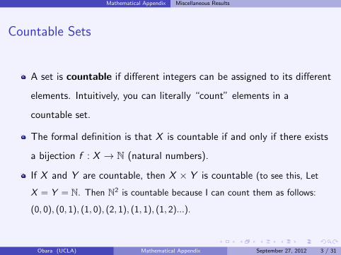
Countable Sets
A set is countable if different integers can be assigned to its different
elements. Intuitively, you can literally “count” elements in a
countable set.
The formal definition is that X is countable if and only if there exists
a bijection f : X → N (natural numbers).
If X and Y are countable, then X × Y is countable (to see this, Let
X = Y = N. Then N2 is countable because I can count them as follows:
(0, 0), (0, 1), (1, 0), (2, 1), (1, 1), (1, 2)...).
Obara (UCLA) Mathematical Appendix September 27, 2012 3 / 31

Mathematical Appendix Miscellaneous Results
sup and inf
For any subset Y of real numbers (Y ⊂ <), there is the smallest
upper bound and the largest lower bound (in <). See any textbook
on analysis (or even “supremum” in Wikipedia) to find the definitions.
Ex. sup {1, 2, 3} = 3, sup {1, 2, 3, ...} =∞, inf(0, 1) = 0. Note that
supY or inf Y may not be in Y .
The following properties follow from the definition almost
immediately.
I For any (nonempty) Y ⊂ <, there exists yn ∈ Y , n = 1, 2, .. such that
yn → supY (the same result applies to inf Y ).
Obara (UCLA) Mathematical Appendix September 27, 2012 4 / 31

Mathematical Appendix Miscellaneous Results
Sequence
A few useful facts about sequences in <L.
If xn, n = 1, 2, is bounded, then there exists a convergent
subsequence.
If xn converges to x∗, then every subsequence of xn converges to x∗.
xn converges to x∗ if and only if x`,n converges to x∗` for every
` = 1, 2, ..., L.
Consider a sequence of numbers (L = 1). We use
lim supn→∞ xn := limn→∞ sup {xm,m ≥ n} and
lim infn→∞ xn := limn→∞ inf {xm,m ≥ n}.I Clearly lim supn→∞ xn ≥ lim infn→∞ xn.
I If lim inf xn ≥ lim sup xn, then lim inf xn = lim sup xn (= lim xn).
Obara (UCLA) Mathematical Appendix September 27, 2012 5 / 31

Mathematical Appendix Miscellaneous Results
Compactness in <n
X ⊂ <n is compact if and only if it is closed and bounded.
Another definition of compactness: X ⊂ <n is compact if and only if
every open cover (i.e. a collection of open sets such that their union
includes X ) of X has a finite cover (i.e. open cover with a finite
number of open sets).
Obara (UCLA) Mathematical Appendix September 27, 2012 6 / 31

Mathematical Appendix Correspondence
2. Correspondence
A map f which maps each point in X ⊂ <M to a subset of Y ⊂ <N
is called correspondence and denoted by f : X ⇒ Y .
We always assume that f (x) is not an empty set for any x ∈ X .
Closed-Graph Property
f : X ⇒ Y has a closed graph if
1 yn ∈ f (xn)
2 xn → x∗ ∈ X
3 yn → y∗
for a sequence (xn, yn) ∈ X × Y , then y∗ ∈ f (x∗).
Obara (UCLA) Mathematical Appendix September 27, 2012 7 / 31

Mathematical Appendix Correspondence
Continuity of Correspondence
upper hemicontinuity
Given X ⊂ <M Y ⊂ <N , f : X ⇒ Y is upper hemicontinuous (uhc) if
its image of every compact set in X is bounded and f has a closed graph.
lower hemicontinuity
Given X ⊂ <M and Y ⊂ <N , f : X ⇒ Y is lower hemicontinuous (lhc)
if for any x∗ ∈ X , any sequence xn ∈ X converging to x∗ and any
y∗ ∈ f (x∗), there exists yn ∈ f (xn) such that yn → y∗.
f : X ⇒ Y is continuous if it is uhc and lhc.
Obara (UCLA) Mathematical Appendix September 27, 2012 8 / 31

Mathematical Appendix Correspondence
Continuity of Correspondence
Comments.
If f is a function, then both uhc and lhc imply continuity in the usual
sense.
The first condition for uhc can be replaced by “f is locally bounded
at every x ∈ X”, i.e. there exists an open neighborhood of x on
which f is bounded (why?).
We say f is uhc at x ∈ X if f is locally bounded at x and satisfies
the closed-graph property at x . f is uhc if and only if f is uhc at
every x ∈ X .
Obara (UCLA) Mathematical Appendix September 27, 2012 9 / 31

Mathematical Appendix Correspondence
Continuity of Correspondence
Show that budget constraint correspondence
B(p,w) ={x ∈ <L
+ : p · x ≤ w}
is continuous in <L++ ×<+.
Constraint for cost minimization problem{x ∈ <L
+ : u(x) ≥ u}
is not
continuous in u (why?). But for any given p � 0, we can modify this
constraint so that the constraint set is locally continuous in (p, u).
I Pick any x ′ such that u(x ′) > u.
I Find x ∈ <+ such that p` x ≥ p′ · x ′ for any ` for any p′ in a
neighborhood of p.
I Then the cost minimizing solution is the same locally even if the
constraint set is replaced by{x ∈ <L
+ : u(x) ≥ u, x` ≤ x ∀`}
, which is
continuous.
Obara (UCLA) Mathematical Appendix September 27, 2012 10 / 31
Mathematical Appendix Maximum Theorem
3. Maximum Theorem
Maximum Theorem
Let F : X × A(⊂ <M ×<N)→ < be a continuous function and
G : A ⇒ X be a continuous correspondence. Let γ(a) ⊂ X be the set of
the solutions for maxx∈G(a) F (x , a) given a ∈ A. Then
(i) γ : A ⇒ X is upper hemicontinuous, and
(ii) V (a) := maxx∈G(a) F (x , a) is continuous in a.
Obara (UCLA) Mathematical Appendix September 27, 2012 11 / 31

Mathematical Appendix Maximum Theorem
Proof of uhc
Since G is uhc, (1) G (a) is compact, hence γ(a) is nonempty, and (2)
γ(a) is locally bounded for every a ∈ A. (2) means that we just need
to prove the closed graph property of γ(a) for each a ∈ A.
Take any sequence (xn, an) ∈ X × A such that xn ∈ γ(an),
an → a∗ ∈ A, and xn → x∗. Note that x∗ ∈ G (a∗) because G is uhc.
Take any x ′ ∈ γ(a∗) and ε > 0. Since G is lhc, there exists
x ′n ∈ G (an) such that x ′n → x ′. Since F is continuous, there exists N
such that F (x ′n, an) ≥ V (a∗)− ε for any n ≥ N. Since xn ∈ γ(an), we
have F (xn, an) ≥ F (x ′n, an). Hence F (x∗, a∗) ≥ V (a∗)− ε by
continuity. Then F (x∗, a∗) ≥ V (a∗) by letting ε→ 0. Therefore
x∗ ∈ γ(a∗).
Obara (UCLA) Mathematical Appendix September 27, 2012 12 / 31
Mathematical Appendix Maximum Theorem
Proof of continuity
Take any sequence an ∈ A such that an → a∗ ∈ A. The previous
proof shows that G is lhc ⇒ lim infn→∞ V (an) ≥ V (a∗).
So we just need to show lim supn→∞ V (an) ≤ V (a∗). Suppose not.
Then there exists ε > 0 and a subsequence (wlog the original
sequence) such that V (an) ≥ V (a∗) + ε.
Take any sequence x ′n ∈ γ(an). Since G is uhc and
{an, n = 1, 2, ..} ⊂ A is compact, {x ′n, n = 1, 2, ..} ⊂ X is bounded.
Hence we can find a subsequence (wlog...) such that lim x ′n → x∗ for
some x∗ (∈ G (a∗) as G is uhc). Then F (x∗, a∗) ≥ V (a∗) + ε holds in
the limit by continuity, which is a contradiction. Hence
lim supn→∞ V (an) ≤ V (a∗).
Obara (UCLA) Mathematical Appendix September 27, 2012 13 / 31

Mathematical Appendix Maximum Theorem
Comment.
The continuity of Walrasian demand correspondences and Hicksian
demand correspondences follow from (i).
The continuity of indirect utility functions and expenditure functions
can be proved by using (ii)
Obara (UCLA) Mathematical Appendix September 27, 2012 14 / 31

Mathematical Appendix Kuhn-Tucker Theorem
4. Kuhn-Tucker Theorem
Let X be an open convex set in <L. Let f : X → < and
gm : X → <,m = 1, ...,M are differentiable functions.
Consider the following problem.
(P): maxx∈X
f (x) s.t. gm(x) ≥ 0 for m = 1, ...,M.
Obara (UCLA) Mathematical Appendix September 27, 2012 15 / 31

Mathematical Appendix Kuhn-Tucker Theorem
Kuhn-Tucker Theorem
Constraint Qualification: Let M(x∗) be the set of binding constraints at
x∗ (i.e. gm(x∗) = 0 for m ∈ M(x∗)). We say that the constraint
qualification (CQ) is satisfied at x∗ ∈ X if either one of the following
conditions is satisfied.
Constraint Qualification
Linear Independence: {∇gm(x∗)|m ∈ M(x∗)} ⊂ <L are linearly
independent.
Slater Condition: There exists x ′ ∈ X that satisfies gm(x ′) > 0 for
all m ∈ M(x∗) and gm are pseudo-concave for all m ∈ M(x∗).
Obara (UCLA) Mathematical Appendix September 27, 2012 16 / 31

Mathematical Appendix Kuhn-Tucker Theorem
Kuhn-Tucker Theorem
Necessity
If x∗ ∈ X solves (P) and the constraint qualification is satisfied at x∗, then
there exists λ ∈ <M+ such that:
(1) ∇f (x∗) +∑M
m=1 λm∇gm(x∗) = 0 (First order conditions),
(2) gm(x∗) ≥ 0 (= 0 if λm > 0) (Complementary slackness conditions).
Sufficiency
Suppose that f is pseudo-concave, gm,m = 1, ...M are all quasi-concave.
If x∗ ∈ X and λ ∈ <M+ satisfies (1) and (2), then x∗ solves (P).
Obara (UCLA) Mathematical Appendix September 27, 2012 17 / 31

Mathematical Appendix Kuhn-Tucker Theorem
Proof
Let’s prove necessity first. Let x∗ ∈ X be an optimal solution of (P).
Consider the following linearized programming problem.
(P∗) : maxx∈X
Df (x∗)(x − x∗) s.t. Dgm(x∗)(x − x∗) ≥ 0 for m ∈ M(x∗).
We need the following lemma.
Lemma
Suppose that the constraint qualification is satisfied at x∗. If x∗ ∈ X is a
solution for (P), then it is also a solution for (P∗).
Obara (UCLA) Mathematical Appendix September 27, 2012 18 / 31
Mathematical Appendix Kuhn-Tucker Theorem
Proof of Lemma:
I Suppose not. Then ∃x ′ ∈ X such that Df (x∗)(x ′ − x∗) > 0 and
Dgm(x∗)(x ′ − x∗) ≥ 0 for all m ∈ M(x∗).
I If CQ is satisfied, then there exists x ′′ ∈ X such that Dgm(x∗)x ′′ > 0
for all m ∈ M(x∗) (prove this for each type of CQ).
I Then x̂ = x ′ + εx ′′ for small ε > 0 satisfies Df (x∗)(x̂ − x∗) > 0 and
Dgm(x∗)(x̂ − x∗) > 0 for all m ∈ M(x∗). This means that for
xα = x∗ + α (x̂ − x∗), f (xα) > f (x∗) and gm(xα) > 0 for all
m = 1, ...,M if α > 0 is small enough. This is a contradiction. So x∗
must be a solution for (P∗).
Obara (UCLA) Mathematical Appendix September 27, 2012 19 / 31

Mathematical Appendix Kuhn-Tucker Theorem
Proof (continued)
By using Farkas’ Lemma, it can be shown that x∗ is a solution for
(P∗)⇔ x∗ satisfies the K-T condition with some λ ∈ <M+ (this step
does not depend on CQ). The proof (only one direction) is in MWG.
Hence x∗ is a solution for (P)⇒ x∗ is a solution for (P∗)⇔ x∗
satisfies the K-T condition with some λ ∈ <M+ .
Obara (UCLA) Mathematical Appendix September 27, 2012 20 / 31

Mathematical Appendix Kuhn-Tucker Theorem
Proof (continued)
For sufficiency, we just need to show that x∗ is a solution for
(P∗) ⇒ x∗ is a solution for (P) when u is pseudo-concave and gm
are quasi-concave for all m ∈ M(x∗). We prove the contrapositive
below.
Suppose that x∗ is not a solution for (P). Then ∃x ′ ∈ X such that
u(x ′) > u(x∗) and gm(x ′) ≥ 0 for all m ∈ M. Since u is
pseudo-concave, gm is quasi-concave and gm(x∗) = 0 for all
m ∈ M(x∗), Du(x∗)(x ′ − x∗) > 0 and Dgm(x∗)(x ′ − x∗) ≥ 0 for all
m ∈ M(x∗). Hence x∗ is not a solution for (P∗).
Obara (UCLA) Mathematical Appendix September 27, 2012 21 / 31

Mathematical Appendix Kuhn-Tucker Theorem
Farkas’ Lemma
What is Farkas’ Lemma?
Farkas’ Lemma
For any a1, ....aM ∈ <N and b ∈ <N+, only one of the following conditions
hold.
1 ∃λm ≥ 0,m = 1, ...,M such that b =∑M
m=1 λmam.
2 ∃y ∈ <N such that y · b > 0 and y · am ≤ 0 for m = 1, ...,M.
Obara (UCLA) Mathematical Appendix September 27, 2012 22 / 31

Mathematical Appendix Kuhn-Tucker Theorem
Farkas’ Lemma
This just means that b is either in A or not in A in the picture below.
a1a2
b(case2)
b(case1)
Ex. M=N=2
A
Obara (UCLA) Mathematical Appendix September 27, 2012 23 / 31

Mathematical Appendix Kuhn-Tucker Theorem
Note on pseudo-concavity
Pseudo-concavity
f : X → < is pseudo-concave if f (x ′) > f (x)⇒ Df (x)(x ′ − x) > 0.
Easy way to check pseudo-concavity? f is pseudo-concave if
I it is concave (for example, linear), or
I it is quasi-concave and ∇f (x) 6= 0 for all x ∈ X .
K-T may not be sufficient without pseudo-concavity.
Example. Consider maxx∈[−1,1] x3. Then x = 0 satisfies the K-T
condition with (λ1, λ2) = (0, 0), but is clearly not optimal. Note that
the objective function is strictly quasi-concave.
Obara (UCLA) Mathematical Appendix September 27, 2012 24 / 31

Mathematical Appendix Envelope Theorem
5. Envelope Theorem
Suppose that
I f and gm depend on some parameter a ∈ A, where A is an open set in
<K .
I an optimal solution for (P) given a is given by a differentiable function
x(a).
I constraint qualification is satisfied at x(a) for every a ∈ A.
Define the optimal value function v : A→ < by v(a) := f (x(a)).
Obara (UCLA) Mathematical Appendix September 27, 2012 25 / 31

Mathematical Appendix Envelope Theorem
Envelope Theorem
We like to compute ∇v(a).
Let’s first consider the simplest case: assume that there is no
constraint (or no constraint is binding). If x(a) is an optimal solution
given a, then FOC is Dx f (x , a) = 0.
Then we have
∇v(a) = ∇f (x(a), a) = Dx f (x , a)Dx(a)+∇af (x(a), a) = ∇af (x(a), a)
This can be generalized to the case with (binding) constraints.
Obara (UCLA) Mathematical Appendix September 27, 2012 26 / 31

Mathematical Appendix Envelope Theorem
Envelope Theorem
Envelope Theorem
Suppose that the binding constraints for (P) do not change in a
neighborhood of a. Then
∇v(a) = ∇af (x(a), a) +∑m
λm∇agm(x(a), a)
, where λm,m = 1, ...,M are the multipliers in the K-T condition.
Obara (UCLA) Mathematical Appendix September 27, 2012 27 / 31
Mathematical Appendix Implicit Function Theorem
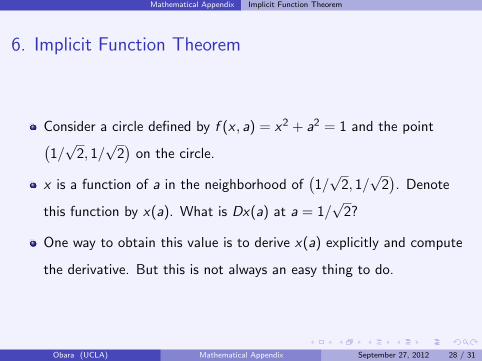
6. Implicit Function Theorem
Consider a circle defined by f (x , a) = x2 + a2 = 1 and the point(1/√
2, 1/√
2)
on the circle.
x is a function of a in the neighborhood of(1/√
2, 1/√
2). Denote
this function by x(a). What is Dx(a) at a = 1/√
2?
One way to obtain this value is to derive x(a) explicitly and compute
the derivative. But this is not always an easy thing to do.
Obara (UCLA) Mathematical Appendix September 27, 2012 28 / 31
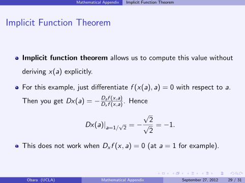
Mathematical Appendix Implicit Function Theorem
Implicit Function Theorem
Implicit function theorem allows us to compute this value without
deriving x(a) explicitly.
For this example, just differentiate f (x(a), a) = 0 with respect to a.
Then you get Dx(a) = −Daf (x ,a)Dx f (x ,a)
. Hence
Dx(a)|a=1/√2 = −
√2√2
= −1.
This does not work when Dx f (x , a) = 0 (at a = 1 for example).
Obara (UCLA) Mathematical Appendix September 27, 2012 29 / 31

Mathematical Appendix Implicit Function Theorem
Implicit Function Theorem
This result generalizes. Let X ∈ <J and A ∈ <K be open sets and
F : X × A→ <J be a C 1 (continuously differentiable) function.
Implicit Function Theorem
If rank DxF (x ′, a′) = J at (x ′, a′) ∈ X × A, then there exist open
neighborhoods V ⊂ X of x ′, U ⊂ A of a′, and a C 1 function f : U → V
such that
1 x = f (a) if and only if F (x , a) = 0 for (x , a) ∈ V × U, and
2 Df (a′) = −DxF (x ′, a′)−1DaF (x ′, a′).
Obara (UCLA) Mathematical Appendix September 27, 2012 30 / 31

Mathematical Appendix Implicit Function Theorem
Implicit Function Theorem
1
1Slope = -1
1/sqrt2
1/sqrt2
U
V
a
x
Obara (UCLA) Mathematical Appendix September 27, 2012 31 / 31