Embed Size (px)
Citation preview

Mathematical Analysis A Concise Introduction
Bernd S. W. Schroder Louisiana Tech University Program of Mathematics and Statistics Ruston, LA
B t C L N T E N N I A L
WILEY-INTERSCIENCE A John Wiley & Sons, Inc., Publication

This Page Intentionally Left Blank
Mathematical Analysis
THE WlLEY BICENTENNIAL-KNOWLEDGE FOR GENERATIONS
ach generation has its unique needs and aspirations. When Charles Wiley first opened his small printing shop in lower Manhattan in 1807, it was a generation of boundless potential searching for an identity. And we were there, helping to define a new American literary tradition. Over half a century later, in the midst of the Second Industrial Revolution, it was a generation focused on building the future. Once again, we were there, supplying the critical scientific, technical, and engineering knowledge that helped frame the world. Throughout the 20th Century, and into the new millennium, nations began to reach out beyond their own borders and a new international community was born. Wiley was there, expanding its operations around the world to enable a global exchange of ideas, opinions, and know-how.
6
For 200 years, Wiley has been an integral part of each generation's journey, enabling the flow of information and understanding necessary to meet their needs and fulfill their aspirations. Today, bold new technologies are changing the way we live and learn. Wiley will be there, providing you the must-have knowledge you need to imagine new worlds, new possibilities, and new opportunities.
Generations come and go, but you can always count on Wiley to provide you the knowledge you need, when and where you need it!
rc'\
WILLIAM J. PESCE U
PETER BOOTH WlLEV PRESIDENT AND CHIEF EXECUTIVE OFFICER CHAIRMAN OF THE BOARD
Mathematical Analysis A Concise Introduction
Bernd S. W. Schroder Louisiana Tech University Program of Mathematics and Statistics Ruston, LA
B t C L N T E N N I A L
WILEY-INTERSCIENCE A John Wiley & Sons, Inc., Publication

Copyright C 2008 by John Wiley & Sons, Inc. All rights reserved
Published by John Wiley & Sons, Inc., Hoboken, New Jersey. Published simultaneously in Canada.
No part of this publication may be reproduced, stored in a retrieval system, or transmitted in any form or by any means, electronic, mechanical, photocopying, recording, scanning, or otherwise, except as permitted under Section 107 or 108 of the 1976 United States Copyright Act, without either the prior written permission of the Publisher, or authorization through payment of the appropriate per-copy fee to the Copyright Clearance Center, Inc., 222 Rosewood Drive, Danvers, MA 01923, (978) 750-8400, fax (978) 750-4470, or on the web at www.copyright.com. Requests to the Publisher for permission should be addressed to the Permissions Department, John Wiley & Sons, Inc., 11 1 River Street, Hoboken, NJ 07030, (201) 748-601 1, fax (201) 748-6008, or online at http://www.wiley.com/go/permission.
Limit of Liability/Disclaimer of Warranty: While the publisher and author have used their best efforts in preparing this book, they make no representations or warranties with respect to the accuracy or completeness of the contents of this book and specifically disclaim any implied warranties of merchantability or fitness for a particular purpose. No warranty may be created or extended by sales representatives or written sales materials. The advice and strategies contained herein may not be suitable for your situation. You should consult with a professional where appropriate. Neither the publisher nor author shall be liable for any loss of profit or any other commercial damages, including but not limited to special, incidental, consequential, or other damages.
For general information on our other products and services or for technical support, please contact our Customer Care Department within the United States at (800) 762-2974, outside the United States at (317) 572-3993 or fax (317) 572-4002.
Wiley also publishes its books in a variety of electronic formats. Some content that appears in print may not be available in electronic format. For information about Wiley products, visit our web site at www.wiley.com.
Wiley Bicentennial Logo: Richard J. Pacific0
Library of Congress Cataloging-in-Publication Data:
Schroder, Bernd S. W. (Bemd Siegfried Walter), 1966- Mathematical analysis : a concise introduction / Bernd S.W. Schroder
ISBN 978-0-470-10796-6 (cloth)
QA300.S376 2007 5 15-dc22
p. cm.
1 . Mathematical analysis. I. Title.
2007024690
Printed in the United States of America.

Contents
Table of Contents V
Preface xi
Part I: Analysis of Functions of a Single Real Variable
1 1 The Real Numbers 1.1 Field Axioms . . . . . . . . . . . . . . . . . . . . . . . . . . . . . . 1 1.2 Order Axioms . . . . . . . . . . . . . . . . . . . . . . . . . . . . . . 4 1.3 Lowest Upper and Greatest Lower Bounds . . . . . . . . . . . . . . . 8 1.4 Natural Numbers, Integers. and Rational Numbers . . . . . . . . . . . 11 1.5 Recursion. Induction. Summations. and Products . . . . . . . . . . . 17
:2 Sequences of Real Numbers 25
25 2.1 Limits . . . . . . . . . . . . . . . . . . . . . . . . . . . . . . . . . . 2.2 Limit Laws . . . . . . . . . . . . . . . . . . . . . . . . . . . . . . . 30 2.3 CauchySequences . . . . . . . . . . . . . . . . . . . . . . . . . . . 36 2.4 Bounded Sequences . . . . . . . . . . . . . . . . . . . . . . . . . . . 40 2.5 Infinite Limits . . . . . . . . . . . . . . . . . . . . . . . . . . . . . . 44
49
3.2 Limit Laws 52
3.4 Continuity 59
:3 Continuous Functions 3.1 Limits of Functions . . . . . . . . . . . . . . . . . . . . . . . . . . . 49
3.3 One-sided Limits and Infinite Limits . . . . . . . . . . . . . . . . . . 56
3.5 Properties of Continuous Functions . . . . . . . . . . . . . . . . . . . 66 3.6 Limits at Infinity . . . . . . . . . . . . . . . . . . . . . . . . . . . . 69
. . . . . . . . . . . . . . . . . . . . . . . . . . . . . . .
. . . . . . . . . . . . . . . . . . . . . . . . . . . . . . . .
71 4 Differentiable Functions 4.1 Differentiability . . . . . . . . . . . . . . . . . . . . . . . . . . . . . 71 4.2 Differentiation Rules . . . . . . . . . . . . . . . . . . . . . . . . . . 74 4.3 Rolle’s Theorem and the Mean Value Theorem . . . . . . . . . . . . 80
V
vi Con tents
5 The Riemann Integral I 5.1 Riemann Sums and the Integral . . . . . . . . . . . . . . . . . . . . . 5.2 Uniform Continuity and Integrability of Continuous Functions . . . . 5.3 The Fundamental Theorem of Calculus . . . . . . . . . . . . . . . . 5.4 The Darboux Integral . . . . . . . . . . . . . . . . . . . . . . . . . .
6 Series of Real Numbers I 6.1 Series as a Vehicle To Define Infinite Sums . . . . . . . . . . . . . . 6.2 AbsoluteConvergenceandUnconditionalConvergence . . . . . . . .
7 Some Set Theory 7.1 The Algebra of Sets . . . . . . . . . . . . . . . . . . . . . . . . 7.2 Countable Sets . . . . . . . . . . . . . . . . . . . . . . . . . . 7.3 Uncountable Sets . . . . . . . . . . . . . . . . . . . . . . . . .
8 The Riemann Integral I1 8.1 Outer Lebesgue Measure . . . . . . . . . . . . . . . . . . . . . . . 8.2 Lebesgue’s Criterion for Riemann Integrability . . . . . . . . . . . 8.3 More Integral Theorems . . . . . . . . . . . . . . . . . . . . . . . 8.4 Improper Riemann Integrals . . . . . . . . . . . . . . . . . . . . .
9 The Lebesgue Integral 9.1 Lebesgue Measurable Sets . . . . . . . . . . . . . . . . . . . . . . . 9.2 Lebesgue Measurable Functions . . . . . . . . . . . . . . . . . . . . 9.3 Lebesgue Integration . . . . . . . . . . . . . . . . . . . . . . . . . . 9.4 Lebesgue Integrals versus Riemann Integrals . . . . . . . . . . . . .
10 Series of Real Numbers I1 10.1 Limits Superior and Inferior 10.2 The Root Test and the Ratio Test 10.3 Power Series . . . . . . . . . . . . . . . . . . . . . . . . . . . . . .
. . . . . . . . . . . . . . . . . . . . . . . . . . . . . . . . . . . . . . . . . .
11 Sequences of Functions 11.1 Notions of Convergence . . . . . . . . . . . . . . . . . . . . . . . . 1 1.2 Uniform Convergence . . . . . . . . . . . . . . . . . . . . . . . . . .
12 Transcendental Functions 12.1 The Exponential Function . . . . . . . . . . . . . . . . . . . . . . . . 12.2 Sine and Cosine . . . . . . . . . . . . . . . . . . . . . . . . . . . . . 12.3 L‘H6pital’s Rule . . . . . . . . . . . . . . . . . . . . . . . . . . . . .
13 Numerical Methods 13.1 Approximation with Taylor Polynomials . . . . . . . . . . . 13.2 Newton’s Method . . . . . . . . . . . . . . . . . . . . . . . 13.3 Numerical Integration . . . . . . . . . . . . . . . . . . . . .
85 85 91 95 97
101 101 108
117 117 122 124
127 127 131 136 140
145 147 153 158 165
169 169 172 175
179 179 182
189 189 193 199
203 204 208 214
Con tents vii
Part 11: Analysis in Abstract Spaces
14 Integration on Measure Spaces 225
14.2 Outer Measures 230
235
242
251
14.1 Measure Spaces . . . . . . . . . . . . . . . . . . . . . . . . . . . . . 225
14.3 Measurable Functions . . . . . . . . . . . . . . . . . . . . . . . . . . 234
14.4 Integration of Measurable Functions . . . . . . . . . . . . . . . . . . 14.5 Monotone and Dominated Convergence . . . . . . . . . . . . . . . . 238
14.6 Convergence in Mean. in Measure. and Almost Everywhere . . . . . . 14.7 Product a-Algebras . . . . . . . . . . . . . . . . . . . . . . . . . . . 245
. . . . . . . . . . . . . . . . . . . . . . . . . . . . .
14.8 Product Measures and Fubini’s Theorem . . . . . . . . . . . . . . . .
15 The Abstract Venues for Analysis 255 15.1 Abstraction I: Vector Spaces . . . . . . . . . . . . . . . . . . . . . . 255 15.2 Representation of Elements: Bases and Dimension . . . . . . . . . . 259
15.3 Identification of Spaces: Isomorphism 15.4 Abstraction 11: Inner Product Spaces 15.5 Nicer Representations: Orthonormal Sets . . . . . . . . . . . . . . . 267 15.6 Abstraction 111: Normed Spaces . . . . . . . . . . . . . . . . . . . . 269 15.7 Abstraction IV: Metric Spaces . . . . . . . . . . . . . . . . . . . . . 275 15.8 LP Spaces . . . . . . . . . . . . . . . . . . . . . . . . . . . . . . . . 278 15.9 Another Number Field: Complex Numbers . . . . . . . . . . . . . . 281
16.1 Convergence of Sequences . . . . . . . . . . . . . . . . . . . . . . . 16.2 Completeness . . . . . . . . . . . . . . . . . . . . . . . . . . . . . . 16.3 Continuous Functions . . . . . . . . . . . . . . . . . . . . . . . . . . 296
16.4 Open and Closed Sets . . . . . . . . . . . . . . . . . . . . . . . . . . 16.5 Compactness . . . . . . . . . . . . . . . . . . . . . . . . . . . . . . 16.6 The Normed Topology of Rd . . . . . . . . . . . . . . . . . . . . . . 16.7 Dense Subspaces . . . . . . . . . . . . . . . . . . . . . . . . . . . . 322
16.9 Locally Compact Spaces . . . . . . . . . . . . . . . . . . . . . . . . 333
. . . . . . . . . . . . . . . . . 262 264 . . . . . . . . . . . . . . . . . .
16 The Topology of Metric Spaces 287 287 29 1
301 309 316
. . . . . . . . . . . . . . . . . . . . . . . . . . . . . 330 16.8 Connectedness
17 Differentiation in Normed Spaces 341 17.1 Continuous Linear Functions . . . . . . . . . . . . . . . . . . . . . . 342 17.2 Matrix Representation of Linear Functions . . . . . . . . . . . . . . . 348 17.3 Differentiability . . . . . . . . . . . . . . . . . . . . . . . . . . . . . 353 17.4 The Mean Value Theorem . . . . . . . . . . . . . . . . . . . . . . . 360 17.5 How Partial Derivatives Fit In . . . . . . . . . . . . . . . . . . . . . 362 17.6 Multilinear Functions (Tensors) . . . . . . . . . . . . . . . . . . . . 369 17.7 Higher Derivatives . . . . . . . . . . . . . . . . . . . . . . . . . . .
17.8 The Implicit Function Theorem . . . . . . . . . . . . . . . . . . . . . 373 380
... Con tents V l l l
18 Measure. Topology. and Differentiation 385 385 391
18.1 Lebesgue Measurable Sets in Rd . . . . . . . . . . . . . . . . . . . . 18.2 Cco and Approximation of Integrable Functions . . . . . . . . . . . . 18.3 Tensor Algebra and Determinants . . . . . . . . . . . . . . . . . . . 397 18.4 Multidimensional Substitution . . . . . . . . . . . . . . . . . . . . . 407
19 Introduction to Differential Geometry 42 1
427
443
19.1 Manifolds . . . . . . . . . . . . . . . . . . . . . . . . . . . . . . . . 421 19.2 Tangent Spaces and Differentiable Functions . . . . . . . . . . . . . . 19.3 Differential Forms. Integrals Over the Unit Cube . . . . . . . . . . . 434 19.4 k-Forms and Integrals Over k-Chains . . . . . . . . . . . . . . . . . . 19.5 Integration on Manifolds . . . . . . . . . . . . . . . . . . . . . . . . 452 19.6 Stokes’ Theorem . . . . . . . . . . . . . . . . . . . . . . . . . . . . 458
20 Hilbert Spaces 463 20.1 Orthonormal Bases . . . . . . . . . . . . . . . . . . . . . . . . . . . 463 20.2 Fourier Series . . . . . . . . . . . . . . . . . . . . . . . . . . . . . . 467 20.3 The Riesz Representation Theorem . . . . . . . . . . . . . . . . . . . 475
Part 111: Applied Analysis
21 Physics Background 483 2 1.1 Harmonic Oscillators . . . . . . . . . . . . . . . . . . . . . . . . . . 484 21.2 Heat and Diffusion . . . . . . . . . . . . . . . . . . . . . . . . . . . 486
2 1.4 Maxwell’s Equations . . . . . . . . . . . . . . . . . . . . . . . . . . 493 21.5 The Navier Stokes Equation for the Conservation of Mass . . . . . . .
22.1 Banach Space Valued Differential Equations . . . . . . . . . . . . . . 22.2 An Existence and Uniqueness Theorem . . . . . . . . . . . . . . . . 508 22.3 Linear Differential Equations . . . . . . . . . . . . . . . . . . . . . .
23.1 Ritz-Galerkin Approximation . . . . . . . . . . . . . . . . . . . . . . 513 23.2 Weakly Differentiable Functions . . . . . . . . . . . . . . . . . . . . 23.3 Sobolev Spaces . . . . . . . . . . . . . . . . . . . . . . . . . . . . . 524 23.4 Elliptic Differential Operators . . . . . . . . . . . . . . . . . . . . . 532 23.5 Finite Elements . . . . . . . . . . . . . . . . . . . . . . . . . . . . . 536
21.3 Separation of Variables. Fourier Series. and Ordinary Differential Equa- tions . . . . . . . . . . . . . . . . . . . . . . . . . . . . . . . . . . . 490
496
22 Ordinary Differential Equations 505 505
510
513
518
23 The Finite Element Method
Conclusion and Outlook 544

Con tents 1x
Appendices
A Logic 545 A.l Statements. . . . . . . . . . . . . . . . . . . . , . . . . . . . . . . . A.2 Negations . . . . . . . . . . . . . . . . . . . . . . . . . . . . . . , .
545 546
B SetTheory 547 B.l The Zermelo-Fraenkel Axioms . . . . . . . . . . . . . . . . . . . . . B.2 Relations and Functions . . . . . . . . . . . . . . . . . . . . . . . . .
547 548
C Natural Numbers, Integers, and Rational Numbers 549 C.1 The Natural Numbers . . , . . , . . . . . . . . . . . . . . . . . . . . C.2 The Integers . . . . . . . . . . . . . . . . . . . . . . . , . . . . . . . C.3 The Rational Numbers . . . . . . . . . . . . . . . . . . . . . . . . .
549 550 550
Bibliography 55 1
Index 553
X
Chapter 5 RlemB"" Integral I
4 Chapter 13 h"lIleClCd
Methods
Con tents
Chapter 8 Chapter I I RlCma""
Integral II Functions + Sequencesof
4 c Chapter 9 Chapter 12 Lcbeigue Trmscendenral Integral F""Ctl0"S
Background: Theon systems Brieflv in Amendices
Chapter 21 Ph>iics
Background
Chapter 6 senes I
I I
Chapter 22 Chapter 21 Ordmay Panial DEr.
Differential Equations Finite Elements
Part I: Analysis on R Counrabdii)
Part 11: Abstract Analysis
Part 111: Applications
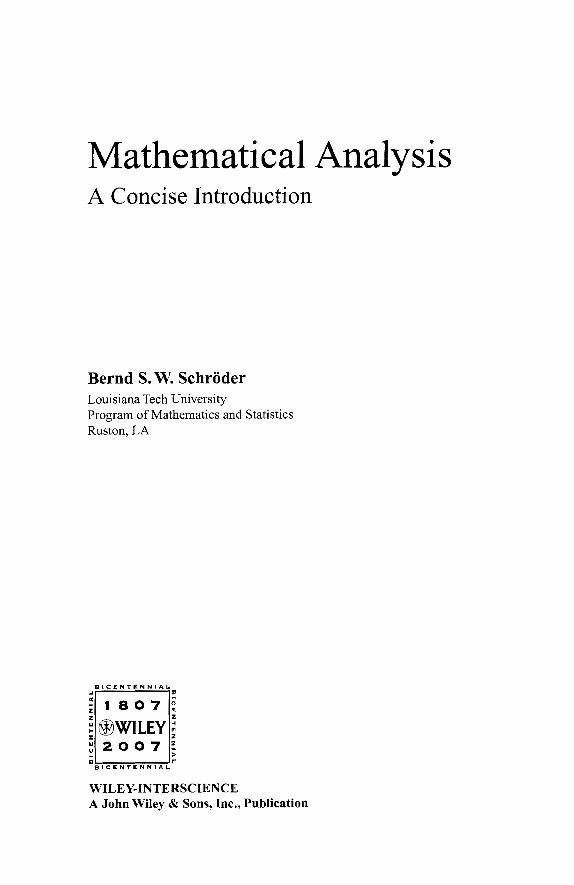
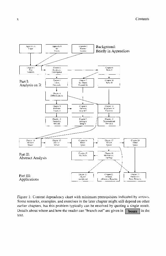
Figure 1 : Content dependency chart with minimum prerequisites indicated by arrows. Some remarks, examples, and exercises in the later chapter might still depend on other earlier chapters, but this problem typically can be resolved by quoting a single result. Details about where and how the reader can "branch out" are given in in the text.
Preface
This text is a self-contained introduction to the fundamentals of analysis. The only prerequisite is some experience with mathematical language and proofs. That is, it helps to be familiar with the structure of mathematical statements and with proof meth- ods, such as direct proofs, proofs by contradiction, or induction. With some support in the right places, mostly in the early chapters, this text can also be used without prerequisites in a first proof class.
Mastering proofs in analysis is one of the key steps toward becoming a mathe- matician. To develop sound proof writing techniques, standard proof techniques are discussed early in the text and for a while they are pointed out explicitly. Throughout, proofs are presented with as much detail and as little hand waving as possible. This makes some proofs (for example, the density of C[a, b] in LP[a, b] in Part 11) notation- ally a bit complicated. With computers now being a regular tool in mathematics, the author considers this appropriate. When code is written for a problem, all details must be implemented, even those that are omitted in proofs. Seeing a few highly detailed proofs is reasonable preparation for such tasks. Moreover, to facilitate the transition to more abstract settings, such as measure, inner product, normed, and metric spaces, the results for single variable functions are proved using methods that translate to these abstract settings. For example, early proofs rely extensively on sequences and we also use the completeness of the real numbers rather than their order properties.
Analysis is important for applications, because it provides the abstract background that allows us to apply the full power of mathematics to scientific problems. This text shows that all abstractions are well motivated by the desire to build a strong theory that connects to specific applications. Readers who complete this text will be ready for all analysis-based and analysis-related subjects in mathematics, including complex analysis, differential equations, differential geometry, functional analysis, harmonic analysis, mathematical physics, measure theory, numerical analysis, partial differential equations, probability theory, and topology. Readers interested in motivation from physics are advised to browse Chapter 21, even if they have not read any of the earlier chapters.
Aside from the topics covered, readers interested in applications should note that the axiomatic approach of mathematics is similar to problem solving in other fields. In mathematics, theories are built on axioms. Similarly, in applications, models are subject to constraints. Neither the axioms, nor the constraints can be violated by the theory or model. Building a theory based on axioms fosters the reader's discipline to not make unwarranted assumptions.
xii Preface
Organization of the content. The text consists of three large parts. Part I, com- prised of Chapters 1-13, presents the analysis of functions of one real variable, includ- ing a motivated introduction to the Lebesgue integral. Chapters 1-6 and 10-13 could be called “single variable calculus with proofs.” For a smooth transition from calculus and a gradual increase in abstraction, Chapters 1-6 require very little set theory. Chap- ter 1 presents the properties of the real line and limits of sequences are introduced in Chapter 2. Chapters 3-5 present the fundamentals on continuity, differentiation, and (Riemann) integration in this order and Chapter 6 gives a first introduction to series.
Chapters 6-8 are motivated by the desire to further explore the Riemann integral while avoiding the excessive use of Riemann sums. This exploration is done with the Lebesgue criterion for Riemann integrability. Although this criterion requires the Lebesgue measure, the payoff is that many proofs become simpler. To quickly reach this criterion, the first presentation of series in Chapter 6 is deliberately kept short. It presents enough about series to allow the definition of Lebesgue measure. Chap- ter 7 presents fundamental notions of set theory. Most of these ideas are needed for Lebesgue measure, but, overall, Chapter 7 contains all the set theory needed in the re- mainder of the text. Chapter 8 finishes the presentation of the Riemann integral. With Lebesgue measure available, it is natural to investigate the Lebesgue integral in Chap- ter 9. This chapter could also be delayed to the end of Part I, but the author believes that early exposure to the crucial ideas will ease the later transition to measure spaces.
The analysis of single variable functions is finished with the rigorous introduc- tion of the transcendental functions. The necessary background on power series is explored in Chapter 10. Chapter 11 presents some fundamentals on the convergence of sequences of functions and Chapter 12 is devoted to the transcendental functions them- selves. Chapter 13 discusses general numerical methods, but transcendental functions provide a rich test bed for the methods presented.
Part I of the text can be read or presented in many orders. Figure 1 shows the prerequisite structure of the text. Prerequisites for each chapter have deliberately been kept minimal. In this fashion, the order of topics in the reader’s first contact with proofs in analysis can be adapted to many readers’ preferences. Most notably, the intentionally early presentation of Lebesgue integration can be postponed to the end of Part I if so desired. Throughout, the author intends to keep the reader engaged by providing motivation for all abstractions. Consequently, as Figure 1 and the table of contents indicate, some concepts and results are presented in a “just-in-time’’ fashion rather than in what may be considered their traditional place. If a concept is needed in an exercise before the concept is “officially” defined in the text, the concept will be defined in the exercise and in the text.
Part 11, comprised of Chapters 14-20, explores how the appropriate abstractions lead to a powerful and widely applicable theoretical foundation for all branches of ap- plied mathematics. The desire to define an integral in d-dimensional space provides a natural motivation to introduce measure spaces in Chapter 14. This chapter facilitates the transition to more abstract mathematics by frequently referring back to correspond- ing results for the one dimensional Lebesgue integral. The proofs of these results usually are verbatim the same as in the one-dimensional setting. Moreover, this early introduction makes LP spaces available as examples for the rest of the text. The ab- stract venues of analysis are then presented in Chapter 15, which provides all examples
... Preface Xll l
for the rest of Part 11. The fundamentals on metric spaces and continuity are presented in Chapter 16. As
with measure spaces, for several results on metric spaces the reader is referred back to the corresponding proof for single variable functions. Proofs are no longer verbatim the same and abstraction is facilitated by translating proofs from a familiar setting to the new setting while analyzing similarities and differences. In a class, the author suggests that the teacher fill in some of these proofs to demonstrate the process.
Chapter 17 presents the fundamentals on normed spaces and differentiation. Again, ideas are similar to those for functions of a single variable, but this time the abstraction goes beyond translation. With all three fundamental concepts (integration, continuity, and differentiation) available in the abstract setting, Chapter 18 shows the interrelation- ship between concepts presented separately before, culminating in the Multivariable Substitution Formula.
The second part is completed by a presentation of the fundamentals of analysis on manifolds, together with a physical interpretation of key concepts in Chapter 19 and by an introduction to Hilbert spaces in Chapter 20.
The remaining chapters give a brief outlook to applied subjects in which analysis is used, specifically, physics in Chapter 21, ordinary differential equations in Chapter 22, and partial differential equations and the finite element method in Chapter 23. Each of these chapters can only give a taste of its subject and I encourage the reader to go deeper into the utterly fascinating applications that lie behind part 111. The mathemati- cal preparation through this text should facilitate the transition.
It should be possible to cover the bulk of the text in a two course sequence. Al- though Chapters 14-16 should be read in order, depending on the available time, the pace and the choice of topics, any of Chapters 17-23 can serve as a capstone experience.
How to read this text. Mathematics in general, and analysis in particular, is not a spectator sport. It is learned by doing. To allow the reader to “do” mathematics, each section has exercises of varying degrees of difficulty. Some exercises require the adaptation of an argument in the text. These exercises are also intended to make the reader critically analyze the argument before adapting it. This is the first step toward being able to write proofs. Of course the need for very critical (and slow) reading of mathematics is nicely summed up in the old quote that “To read without a pencil is daydreaming.” The reader should ask himherself after every sentence “What does this mean? Why is this justified?’ Making notes in the margin to explain the harder steps will allow the reader to answer these questions more easily in the second and third readings of a proof. So it is important to read thoroughly and slowly, to make notes and to reread as often as needed. The extensive index should help with unknown or forgotten terminology as necessary. Other exercises have hints on how to create a proof that the reader has not seen before. These exercises require the use of proof techniques in a new setting. Finally, there are also exercises without hints. Being able to create the proof with nothing but the result given is the deepest task in a mathematics course. This is not to say that exercises without hints are always the hardest and adaptations are always the easiest, but in many cases this is true. Finally, some exercises give a sequence of hints and intermediate results leading up to a famous theorem or a specific example. These exercises could also be used as mini-projects. In a class, some of them
xiv Preface
could be the basis for separate lectures that spotlight a particular theorem or example. To get the most out of this text, the reader is encouraged to not look for hints and
solutions in other background materials. In fact, even for proofs that are adaptations of proofs in this text, it is advantageous to try to create the proof without looking up the proof that is to be adapted. There is evidence that the struggle to solve a problem, which can take days for a single proof, is exactly what ultimately contributes to the development of strong skills. “Shortcuts,” while pleasant, can actually diminish this development. Readers interested in quantitative evidence that shows how the struggle to acquire a skill actually can lead to deeper learning may find the article [4] quite enlightening. A better survival mechanism than shortcuts is the development of con- nections between newly learned content and existing knowledge. The reader will need to find these connections to hisher existing knowledge, but the structure of the text is intended to help by motivating all abstractions. Readers interested in how knowledge is activated more easily when it was learned in a known context may be interested in the article [5] .
Acknowledgments. Strange as it may sound, I started writing this text in the spring of 1987, as I prepared for my oral final examination in the traditional Analysis I- 111 sequence in Germany. Basically, I took all topics in the sequence and arranged them in what was the most logical fashion to me at the time. Of course, these notes are, in retrospect, immature. But they did a lot to shape my abilities and they were a good source of ideas and exercises. In this respect, I am indebted to my teachers for this sequence: Professor Wegener and teaching assistant Ms. Lange for Analysis I, Professor Kutzler and teaching assistant Herr Bottger for Analysis 11-111 as well as Professor Herz in whose Differential Equations class I first saw analysis “at work.” With all due respect to the other individuals, to me and many of my fellow students, the force that drove us in analysis (and beyond) was Herr Bottger. This gentleman was uncompromising in his pursuit of mathematical excellence and we feared as well as looked forward to his demanding exercise sets. He was highly respected because he was ready to spend hours with anyone who wanted to talk mathematics. Those who kept up with him were extremely well prepared for their mathematical careers. Incidentally, Dr. Ansgar Jungel, whose notes I used for the chapter on the finite element method, took the above mentioned classes with me. The thorough preparation through these classes is the main reason why most of this text was comparatively easy to write. If this text does half as good a job as Herr Bottger did with us, it has more than achieved its purpose.
It was thrilling to test my limitations, it was humbling to find them and ultimately I was left awed once more by the beauty of mathematics. When my abilities were in- sufficient to proceed, I used the texts listed in the bibliography for proofs, hints or to structure the presentation. To make the reader fully concentrate on matters at hand, and to force myself to make the exposition self-contained, outside references are limited to places where results were beyond the scope of this exposition. A solid foundation will allow readers to judiciously pick their own resources for further study. Nonetheless, it is appropriate to recognize the influence of the works of a number of outstanding indi- viduals. I used Adams [2], Renardy and Rogers [23], Yosida [33] and Zeidler [34] for Sobolev spaces, Aris 131, Cramer’s http: //www. navier-stokes .net/, and
Preface xv
Welty, Wicks and Wilson [31] for fluid dynamics, Chapman [6] for heat transfer, Cohn [7] for measure theory, DieudonnC [8] for differentiation in Banach spaces, Dodge [9] and Halmos [ 131 for set theory, Ferguson [ 101, Sandefur [24] and Stoer and Bulirsch [28] for numerical analysis, Halliday, Resnick and Walker [ 121 for elementary physics, Hewitt and Stromberg [14], Heuser [15], [16], Johnsonbaugh and Pfaffenberger [20], Lehn [22] and Stromberg [29] for general background on analysis, Heuser [17] for functional analysis, Hurd and Loeb [18] for the use of quantifiers in logic, Jiingel [21] and Solin [25] for the finite element method, Spivak [26], [27] for manifolds, Torchin- sky [30] for Fourier series, Willard [32] for topology, and the Online Encyclopaedia of Mathematics http : / /eom. springer. de/ for quick checks of notation and defi- nitions. Readers interested in further study of these subjects may wish to start with the above references.
The first draft of the manuscript was used in my analysis classes in the Winter and Spring quarters of 2007. The first class covered Chapters 1-9, the second covered Chapters 11 and 14-18 (with some strategic “fast forwards”). This setup assured that graduating students would have full exposure to the essentials of analysis on the real line and to as much abstract analysis as possible without “handwaving arguments.” I am grateful to the students in these classes for keeping up with the pace, solving large numbers of homework problems, being patient with the typos we found and also for suggesting at least one order in which to present the material that I had not considered. The students’ evaluations (my best ever) also reaffirmed for me that people will enjoy, or at least accept and honor, a challenge, and that an ambitious, motivated course should be the way to go. Devery Rowland once more did an excellent job printing drafts of the text for the classes.
Aside from the referees, several colleagues also commented on this text and I owe them my thanks for making it a better product. In particular, I would like to thank Na- talia Zotov for some comments on an early version that significantly improved the pre- sentation, and Ansgar Jiingel for pointing out some key references on Sobolev spaces. Although I hope that we have found all remaining errors and typos, any that remain are my responsibility and mine alone. I request readers to report errors and typos to me so I can post an errata. My contacts at Wiley, Susanne Steitz, Jacqueline Palmieri, and Melissa Yanuzzi bore with me when the stress level rose and their patience made the publishing process very smooth.
As always, this work would not have been possible without the love of my family. It is truly wonderful to be supported by individuals who accept your decision to spend large amounts of time reliving your formative years.
Finally, I was sad to learn that Herr Bottger died unexpectedly a few years after I had my last class with him. Sir, this one’s for you.
Ruston, LA, August 30,2007
Bernd Schroder
Part I
Analysis of Functions
of a Single Real Variable

Chapter 1
The Real Numbers
This investigation of analysis starts with minimal prerequisites. Regarding set theory, the terms “set” and “element” will remain undefined, as is customary in mathematics to avoid paradoxes. The empty set 0 is the set that has no elements. The statement “e E S” says that e is an element of the set S. The statement “ A G B” says that every element of A is an element of B. Sets A and B are equal if and only if A C B and B C A . The statement “A c B” says that A E B and A # B. Subsets will be defined as “ A = {x E S : (property)},” that is, with a statement from which set S the elements of A are taken and a property describing them. The union of two sets A and B is A U B = {x : x E A o r x E B } , theintersectionis A n B = {x : x E A andx E B ) .
Union and intersection of finitely many sets are denoted u A j and n A j , respec-
tively, and the relative complement of B in A is A \ B = {x E A : x @ B ) . Further details on set theory are purposely delayed until Section 7.1. Until then, we focus on analytical techniques. Any required notions of set theory will be clarified on the spot.
To define properties, sometimes the universal quantifier “V” (read “for all”) or the existential quantifier “3” (read “there exists”) are used. Formal logic is described in more detail in Appendix A. Finally, the reader needs an intuitive idea what a function, a relation and a binary operation are. Details are relegated to Appendices B.2 and C.2.
The real numbers R are the “staging ground” for analysis. They can be charac- terized as the unique (up to isomorphism) mathematical entity that satisfies Axioms 1.1, 1.6, and 1.19. That is, they are the unique linearly ordered, complete field (see Exercise 1-30). In this chapter, we introduce the axioms for the real numbers and some fundamental consequences. These results assure that the real numbers indeed have the properties that we are familiar with from algebra and calculus.
n n
j = l j = 1
1.1 Field Axioms
The description of the real numbers starts with their algebraic properties.
1
2 1. The Real Numbers
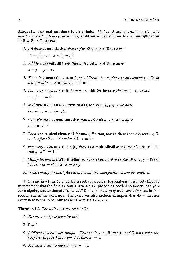
Axiom 1.1 The real numbers R are a field. That is, R has at least two elements and there are two binary operations, addition + : R x R + R and multiplication . : R x R -+ R, so that
1. Addition is associative, that is, for all x , y , z E R we have
(x + y ) + z = x + ( y + z ) .
2. Addition is commutative, that is, for all x , y E R we have
x + y = y + x .
3. There is a neutral element 0 for addition, that is, there is an element 0 E R so tha t fora l lx E R we havex + 0 = x .
4. For every element x E R there is an additive inverse element (-x) so that
x + (-x) = 0.
5. Multiplication is associative, that is, for all x , y, z E R we have
(x . y ) . z = x . ( y . z ) .
6. Multiplication is commutative, that is, for all x , y E R we have
x ‘ 4 ’ = y .x.
7. There is a neutral element 1 f o r multiplication, that is, there is an element 1 E R so that for all x E R we have 1 . x = x .
8. For every element x E R \ {0} there is a multiplicative inverse element x - l so tha tx . x - l = 1.
9. Multiplication is (left) distributive over addition, that is, for all a , x , y E R we have a . (x + y) = a, .x + a . y.
As is customary for multiplication, the dot between factors is usually omitted.
Fields are investigated in detail in abstract algebra. For analysis, it is most effective to remember that the field axioms guarantee the properties needed so that we can per- form algebra and arithmetic “as usual.” Some of these properties are exhibited in this section and in the exercises. The exercises also include examples that show that not every field needs to be infinite (see Exercises 1-7-1-9).
Theorem 1.2 The following are true in R:
1. For all x E R, we have Ox = 0.
2. 0 # 1.
3. Additive inverses are unique. That is, i f x E R and x’ and X both have the property in part 4 ofAxiom 1.1, then x’ = X.
4. For all x E R, we have (- l)x = -x.
1.1. Field Axioms 3
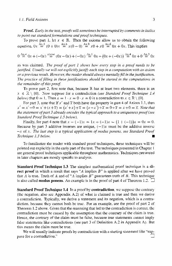
Proof. Early in the text, proofs will sometimes be interrupted by comments in italics
To prove part 1, let x E R. Then the axioms allow us to obtain the following to point out standard formulations and proof techniques.
equation. Ox = (O+O)x = x(O+O) = xO+xO = Ox +Ox. This implies Ax.3 Ax.6 Ax.9 Ax.6
as was claimed. The proof of part I shows how every step in a proof needs to be just$ed. Usually we will not explicitly justify each step in a computation with an axiom or a previous result. Howevel; the reader should always mentally fill in the justi3cation. The practice of filling in these justiJcations should be started in the computations in the remainder of this proot
To prove part 2, first note that, because R has at least two elements, there is an x E R \ (0) . Now suppose for a contradiction (see Standard Proof Technique 1.4 below) that 0 = 1. Then x = 1 . x = 0 . x = 0 is a contradiction to x E R \ (0) .
For part 3, note that if x’ and X both have the property in part 4 of Axiom 1.1, then x’ = x’+O = x’+(x+X) = (x’+x)+X = (x+x’)+X = O+X = X+O = X. Note that the statement of part 3 already encodes the typical approach to a uniqueness proof (see Standard Proof Technique 1.5 below).
Finally, for part 4 note that x + (- l ) x = l x + (- 1)x = (1 + (- 1)). = Ox = 0. Because by part 3 additive inverses are unique, (- l)x must be the additive inverse -x of x . The last step is a typical application of modus ponens, see Standard Proof Technique 1.3 below.
To familiarize the reader with standard proof techniques, these techniques will be pointed out explicitly in the early part of the text. The techniques presented in Chapter 1 are general proof techniques applicable throughout mathematics. Techniques presented in later chapters are mostly specific to analysis.
Standard Proof Technique 1.3 The simplest mathematical proof technique is a di- rect proof in which a result that says “ A implies B” is applied after we have proved that A is true. Truth of A and of “ A implies B” guarantees truth of B. This technique is also called modus ponens. An example is in the proof of part 4 of Theorem 1.2. 0
Standard Proof Technique 1.4 In a proof by contradiction, we suppose the contrary (the negation, also see Appendix A.2) of what is claimed is true and then we derive a contradiction. Typically, we derive a statement and its negation, which is a contra- diction, because they cannot both be true. For an example, see the proof of part 2 of Theorem 1.2 above. Given that the reasoning that led to the contradiction is correct, the contradiction must be caused by the assumption that the contrary of the claim is true. Hence, the contrary of the claim must be false, because true statements cannot imply false statements like contradictions (see part 3 of Definition A.2 in Appendix A). But this means the claim must be true.
We will usually indicate proofs by contradiction with a starting statement like “sup- pose for a contradiction.” 0
4 1. The Real Numbers
Standard Proof Technique 1.5 For many mathematical objects it is important to as- sure that they are the only object that has certain properties. That is, we want to assure that the object is unique. In a typical uniqueness proof, we assume that there is more than one object with the properties under investigation and we prove that any two of these objects must be equal. Part 3 of Theorem 1.2 shows this approach.
Exercises 1-1. Prove that ( -1) . (-1) = 1.
1-2. . is right distributive over +. Prove that for all x , y , z E R we have (x + y ) z = xz + yz.
1-3. Multiplicative inverses are unique. Prove that if x E W and x' and X both have the property in part 8 of Axiom 1.1 then x' = X.
1-4. Prove that 0 does not have a multiplicative inverse.
1-5. Prove that if x , y # 0, then ( x y ) - ' = y - l x - ' . Conclude in particular that x y # 0.
1-6. Prove each of the binomial formulas below. Justify each step with the appropriate axiom
(a) (a + b)2 = a* + 2ab + b2
(c) (a + b)(a - b ) = a2 - b2
(b) (a - b)* = a2 - 2ab + b2
1-7. Prove that the set (0, 1) with the usual multiplication and the usual addition, except that 1 + 1 := 0, is a field. That is, prove that the set and addition and multiplication as stated have the properties listed in Axiom 1.1.
1-8. Prove that the set (0, 1. 2) with the sum and product of two elements being the remainder obtained when dividing the regular sum and product by 3 is a field.
1-9. A property and some finite fields
(a) Let F be a field and let x , y E F . Prove that x y = 0 if and only if x = 0 or y = 0
(b) Prove that the set [O. 1, 2. 3 ) with the sum and product of two elements being the remainder obtained when dividing the regular sum and product by 4 is not a field.
(c) Prove that the set (0, 1, . , , , p - 1) with the sum and product of two elements being the remainder obtained when dividing the regular sum and product by p is a field if and only if p is a prime number.
1.2 Order Axioms
Exercises 1-7-1-9c show that the field axioms alone are not enough to describe the real numbers. In fact, fields need not even be infinite. However, aside from executing the familiar algebraic operations, we can also compare real numbers. This section presents the order relation on the real numbers and its properties.
Axiom 1.6 The real numbers R contain a subset R+, called the positive real numbers such that
1. For all x , y E R+, we have x + y E E%+ and x y E E%+,
2. For all x E R, exactly one of the following three properties holds.
Either x E R+ or -x E Rt or x = 0.
1.2. Order Axioms 5
A real number x is called negative if and only if -x E R+. Once positive numbers are defined, we can define an order relation. As usual,
instead of writing y + (-x) we write y - x and call it the difference of x and y. The binary operation “-” is called subtraction.
The phrase “if and only if,” which is used in definitions and biconditionals, is nor- mally abbreviated with the artificial word “iff.”
Definition 1.7 For x, y E R, we say x is less than y, in symbols x < y, i f f y -x E R+. We say x is less than or equal to y, denoted x 5 y, ifSx < y or x = y. Finally, we say x is greater than y, denoted x > y, i r y < x, and we say x is greater than or equal to y , denoted x 2 y, ifsy 5 x.
The relation 5 satisfies the properties that define an order relation.
Proposition 1.8 The relation 5 is an order relation on R. That is,
1. 5 is reflexive. For all x E R we have x 5 x,
2. 5 is antisymmetric. For all x, y E R we have that x 5 y and y 5 x implies x = y,
3. 5 is transitive. For all x, y , z E X , we have that x 5 y and y 5 z implies x 5 z.
Moreovel; the relation 5 is a total order relation, that is, for any two x, y E R we have that x 5 y or y 5 x.
Proof. The relation 5 is reflexive, because it includes equality. For antisymmetry, let x 5 y and y 5 x and suppose for a contradiction that x + y.
Then x - y E R+ and -(x - y ) = y - x E R+, which cannot be by Axiom 1.6. Thus - < must be antisymmetric.
For transitivity, let x 5 y and y 5 z . There is nothing to prove if one of the inequalities is an equality. Thus we can assume that x y and y < z , which means y - x E Rf and z - y E R+. But then R+ contains (7, - y) + ( y - x) = z - x, and hence x < z . We have shown that for all x, y. z E R the inequalities x 5 y and y I: z imply x 5 z , which means that 5 is transitive.
For the “moreover” part note that if x, y E R, then y - x E R and we have either y - x E R+, which means x < y , or y - x = 0, which means y = x, or x - y = - (y-x) ER+,whichmeansy <x. Thereforeforallx,y E R o n e o f x 5 y or y 5 x holds, and hence 5 is a total order.
Once an order relation is established, we can define intervals.
Definition 1.9 An interval is a set I C R so that for all c , d E I and x E R the inequalities c < x < d imply x E I . In particular for a , b E R with a < b we define
1. [a , b] := (X E R : a 5 x 5 b},
2. ( a , b ) := (x E R : a < x < b] , ( a , 00) := (x E R : a < x}, (-00. b ) := (X E R : x < b}, (-w, 00) := R,

6 1. The Real Numbers
3. [a , b ) := {x E R : a 5 x < b} , [a , 00) := { X E R : u 5 x},
4. ( a , b ] := {X E R : u < x 5 b ] , (-w, b ] := ( X E R : x 5 b].
The points a and b are also called the endpoints of the interval. An interval that does not contain either of its endpoints (where &m are also considered to be "end- points") is called open, An interval that contains exactly one of its endpoints is called half-open and an interval that contains both its endpoints is called closed.
For the first part of this text, the domains of functions will almost exclusively be intervals. Because analysis requires extensive work with inequalities, we need to in- vestigate how the order relation relates to the algebraic operations.
Theorem 1.10 Properties of the order relation. Let x , y , z E R.
1. The number x is positive i f sx > 0 and x is negative c r x < 0.
2. I f x 5 y , then x + z 5 y + z .
3. I f x 5 y and z > 0, then xz 5 y z .
4. I f x 5 y and z < 0, then xz 2 yz .
5. l f 0 < x 5 y , then y-' 5 x-'.
Similar results can be proved for other combinations of strict and nonstrict inequalities. We will not state these here, but instead trust that the reader can make the requisite translation from the statements in this theorem.
Proof. Parts 1 and 2 are left to the reader as Exercises 1-10a and 1-lob. Throughout this text, parts of proofs will be delegated to the reader to facilitate a better connection to the material presented.
For part 3 , let x 5 y and let z > 0. Then, y - x E R+ or y = x. In case y = x, we obtain y z = x z and thus, in particular, xz 5 yz . In case y - x E R+, note that z > 0 means z E R+, and hence y z - xz = ( y - x ) z E R+. By definition, this implies xz < y z , and in particular xz 5 yz . Because we have shown xz 5 y z in each case, the result is established. All proofs in this section are done with the above kind of case distinction (see Standard Proof Technique 1.1 1).
For part 4, let x 5 y and let z < 0. Then, y - x E R+ or y = x. In case y = x, we obtain y z = x z , and hence xz 2 y z . In case y - x E Rf, note that z < 0 means -2 E B+, and hence xz - yz = ( x - y ) z = ( y - x ) ( - z ) E R+. By definition, this implies y z < xz, and hence y z 5 xz, which establishes the result.
For part 5, first note that there is nothing to prove if x = y . Hence, we can assume that x < y . Suppose for a contradiction that x - l < y-' . Then by part 3 we have that
Standard Proof Technique 1.11 When several possibilities must be considered in a proof, the proof usually continues with separate arguments for each possibility. The proof is complete when each separate argument has led to the desired conclusion. This
1 = x - l x < y - ' x , and hence x < y . 1 < y y - ' x = x, contradiction.
type of proof is also called a proof by case distinction. 0
1.2. Order Axioms 7
We conclude this section by introducing the absolute value function and some of its properties.
Definition 1.12 For x E R, we set Ix I =
value of x .
x; i f x 1.0, -x; i f x < 0,
and we call it the absolute
Theorem 1.13 summarizes the properties of the absolute value. The numbering is adjusted so that properties 1 ,2 , and 3 correspond to the analogous properties for norms (see Definition 15.38). We will formulate many results in the jirst part of the text to be analogous or easily generalizable to more abstract settings, but we will usually do so without explicit forward references. In this fashion many abstract situations will be more familiar because of similarities to situations investigated in the jirst part.
Theorem 1.13 Properties of the absolute value.
0. For all x E R, we have Ix I > 0,
1. For all x E R, we have 1x1 = 0 i y x = 0,
2. F o r a l l x , y ER, wehave lxyl = Ixllyl,
3. Triangular inequality. For all x, y E R, we have Ix + y I 5 lx I + I y 1 .
4. Reverse triangular inequality. For all x , y E R, we have 1 Ix I - I y I 1 I Ix - y I .
Proof. For part 0, let x E R. In case x > 0, by Definition 1.12 we have /x 1 = x > 0. In case x < 0, we have x @ R+ and by part 2 of Axiom 1.6 we conclude -x > 0. Because in this case Ix I = -x > 0, part 0 follows.
Throughout the text, the two implications of a biconditional “ A iff B” will be re- ferred to as “+,” denoting “if A, then B ” and “+,” denoting “if B, then A.”
For part 1, note that the direction “+=” is trivial, because (01 = 0. For the direction “j,” let x E R be so that /x I = 0 and suppose for a contradiction that x + 0. If x > 0, then 0 < x = 1x1 = 0, a contradiction. (Note that the previous sentence is a shortproof by contradiction that is part of a longer proof by contradiction.) Therefore x < 0. But then 0 < -x = 1x1 = 0, a contradiction. Hence, x must be equal to 0.
For part 2 , let x , y E R. If x 2 0 and y 1. 0, then by part 3 of Theorem 1.10 xy 1. 0, and hence lxyl = x y = I x / / y l . If x 2 0 and y < 0, then by part 4 of Theorem 1.10 we infer xy 5 0. Hence, (xyl = -xy = x ( - y ) = JxJJyJ . The case x < 0 and y 3 0 is similar and the reader will produce it in Exercise 1 - 1 1 a. Finally, if x < 0 and y < 0, then by part 4 of Theorem 1.10 we obtain x y > 0. Hence,
To prove the triangular inequality, first note that for all x E IR we have that x I /x 1 . This is clear for x 1. 0 and for x < 0 we simply note x < 0 < -x = 1x1. Moreover, (see Exercise 1- l lb) for all x E R we have -x I 1x1. Now let x, y E R. If the inequality x + y 2 0 holds, then by part 2 of Theorem 1.10 at least one of x. 4’ is greater than or equal to 0. (Otherwise x < 0 and y < 0 would imply x + y < 0.) Hence,bypart2ofTheoreml.lOIx+yI = x + y l I x l + y ~ I x I+Iy I . I f x+y ( 0 ,
/xyl = xy = (-l)(-1)xy = ( - x ) ( - y ) = ixl ly l .

8 1. The Real Numbers
then at least one of x and y is less than 0. Hence, by part 2 of Theorem 1.10 we obtain
Finally, for the reverse triangular inequality, let x, y E R. Without loss of generality (see Standard Proof Technique 1.14) assume that ( X I 3 IyI. (The proof for the case 1x1 < lyl is left as Exercise 1-llc.) Then 1x1 = Ix - y + yl i Ix - yI + lyl, which
w
Ix + yl = -(x + y ) = --x + ( - y ) - < I - X I + ( - Y ) i I - - X I + I - Y I = 1x1 + IYI .
implies 11x1 - 1y11 = 1x1 - IYI i Ix - Y I .
Standard Proof Technique 1.14 If the proofs for the cases in a case distinction are very similar, it is customary to assume without loss of generality that one of these similar cases is true. This is not a loss of generality, because it is assumed that what is presented enables the reader to fill in the proof(s) for the other case(s). In this text, the omitted part is sometimes included as an explicit exercise for the reader. 0
Exercises 1- 10. Finishing the proof of Theorem 1.10
(a) Prove part 1 of Theorem 1.10.
(b) Prove part 2 of Theorem 1.10.
1-1 1. Finishing the proof of Theorem 1.13.
(a) L e t x , y ~ W . P r o v e t h a t i f x > O a n d y ~ O , t h e n I x y l = I x l l y l .
(b) Prove that for all x E R we have --x 5 1x1.
(c) Prove that if 1x1 < Iyl , then 11x1 - ( y / 1 5 Ix - y / .
1-12. Let I , J G R be intervals. Prove that I n J = { x E W : x E I and x E J ] is again an interval
1-13. Let a < b and le tx , y E [u , b]. Prove that In - yI 5 b - a
1-14. Prove that none of the fields from Exercise 1-9c can satisfy Axiom 1.6 by showing that for these fields part 2 of Axiom 1.6 fails for n = 1. Note. This result shows that Axiom 1.6 distinguishes R from the finite fields of Exercise 1-9c.
1.3 Lowest Upper and Greatest Lower Bounds
A structure that has the properties outlined in Axioms 1.1 and 1.6 is also called a linearly ordered field. The rational numbers satisfy these properties just as well as the real numbers. Thus we are not done with our characterization of R. The final axiom for the real numbers addresses upper and lower bounds of sets.
Definition 1.15 Let A be a subset ofR.
1. The number u E R is called an upper bound of A iff u 2 a for all a E A. If A has an upper bound, it is also called bounded above.
2. The number I E R is called a lower bound of A i f f 1 5 a fo r all a E A. If A has a lower bound, it is also called bounded below.
A subset A R that is bounded above and bounded below is also called bounded.
1.3. Lowest Upper and Greatest Lower Bounds 9
Among all upper bounds of a set, the smallest one (if it exists) plays a special role. Similarly, the greatest lower bound plays a special role if it exists.
Definition 1.16 Let A C R.
1. The number s E R is called lowest upper bound of A or supremum of A, denoted sup(A), iffs is an upper bound of A and for all upper bounds u of A we have that s 5 u.
2. The number i E R is called greatest lower bound of A or infimum of A, de- noted inf(A), iff i is a lower bound of A and for all lower bounds 1 of A we have that 1 5 i .
Formally, it is not guaranteed that suprema and infima are unique, but the next result shows that this is indeed the case. Note that the statement of Proposition 1.17 follows the standard pattern for a uniqueness statement.
Proposition 1.17 Suprema are unique. That is, i f the set A and s , t E R both are suprema of A, then s = t .
R is bounded above
Proof. Let A G Iw and s, t E R be as indicated. Then s is an upper bound of A and, because t is a supremum of A, we infer s 2 t . Similarly, t is an upper bound of A and,
Standard Proof Technique 1.18 (Also compare with Standard Proof Technique 1.14.) When, as in the proof of Proposition 1.17, two parts of a proof are very similar, it is common to only prove one part and state that the other part is similar. Throughout the text, the reader will become familiar with this idea through exercises that require the
because s is a supremum of A, we infer t 2 s. This implies s = t .
construction of proofs that are similar to proofs given in the narrative.
The proof that infima are unique is similar (see Exercise 1-15). Because suprema
The final axiom for the real numbers now states that suprema and infima exist under and infima are unique if they exist, we speak of the supremum and the infimum.
mild hypotheses.
Axiom 1.19 Completeness Axiom. Every nonempty subset S of R that has an upper bound has a lowest upper bound.
Although the Completeness Axiom formally only guarantees that nonempty subsets of R that are bounded above have suprema, existence of infima is a consequence.
Proposition 1.20 Let S 5 R be nonempty and bounded below. Then S has a greatest lower bound.
Proof. Let L := {x E R : x is a lower bound of S}. Then L f 0. Let s E S. Then for all 1 E L we have that 1 I s. Because S f: 0 this means that L is bounded above. Because L f: 0, by the Completeness Axiom, L has a supremum sup(L). Every s E S is an upper bound of L, which means that s 2 sup(L) and so sup(L) is a lower bound of S . By definition of suprema, sup(L) is greater than or equal to all elements of L ,
10 1. The Real Numbers
that is, it is greater than or equal to all lower bounds of S. By definition of infima, this rn
We will see that suprema and infima are valuable tools in analysis on the real line. The next result shows that in any set with a supremum we can find numbers that are arbitrarily close to the supremum. This fact is important, because analysis ultimately is about objects “getting close to each other.”
Proposition 1.21 Let S c R be a nonempty subset of R that is bounded above and let s := sup(S). Then for every E > 0 there is an element x E S so that s - x < E.
Proof. Suppose for a contradiction that there is an E > 0 so that for all x E S we have that s - x 1 E . Then for all x E S we would obtain s - E 1 x, that is, s - E would be an upper bound of S. But s - E < s contradicts the fact that s is the lowest upper bound of S. rn
Although the supremum and infimum of a set need not be elements of the set, we
means that sup(L) = inf(S).
have different names for them in case they are in the set.
Definition 1.22 Let A be a subset of R.
1. If A is bounded above and sup(A) E A, then the supremum of A is also called the maximum of A, denoted max(A).
minimum of A, denoted min(A). 2. If A is bounded below and inf(A) E A, then the injmum of A is also called the
Although the distinctions between suprema and maxima and between infima and minima are small, the notions are distinct. For example, the open interval (0, 1) has a supremum (1) and an infimum (0), but it has neither a maximum, nor a minimum.
Exercises 1-15. Let A g W be bounded below and le ts , f E W both be infima of A. Prove that s = t .
1-16. Approaching infima. State and prove a version of Proposition 1.21 that applies to infima. Is the proof significantly different from that of Proposition 1.21?
1-17. Let S g W be bounded above. Prove that s E W is the supremum of S iff s is an upper bound of S and for all E > 0 there is an x E S so that Is - x / < E .
1-18. Suprema and infima vs. containment of sets.
(a) Let A. B C W be bounded above. Prove that A 5 B implies sup(A) 5 sup(B).
(b) Let A , B g W be bounded below. Prove that A g B implies inf(A) ? inf(B).
1-19. Let A g W be bounded above. Prove that inf(x E R : - x E A] = - sup(A).

1.4. Natural Numbers, Integers, and Rational Numbers 11
1.4 Natural Numbers, Integers, and Rational Numbers
Although Axioms 1.1, 1.6 and 1.19 uniquely describe the real numbers, they do not mention familiar subsets, such as natural numbers, integers, and rational numbers. This is because these sets can be constructed from the axioms as subsets of the real numbers. We start with the natural numbers, which are the unique subset with properties as stated in Theorem 1.23. While their existence is easy to establish, the uniqueness of the natural numbers can only be proved in Theorem 1.28 after some more machinery has been developed.
Theorem 1.23 There is a subset N G R, called the natural numbers, so that
1. 1 E N .
2. For each n E N the number n + 1 is also in N.
3. Principle of Induction. If S s N is such that 1 E S and for each n E S we also have n + 1 E S, then S = N.
Proof. Call a subset A G R a successor set iff 1 E A and for all a E A we also have a + 1 E A . Successor sets exist, because, for example, R itself is a successor set. Let N be the set of all elements of R that are in all successor sets. Because 1 is an element of every successor set, we infer 1 E N. Moreover, if n E N, then n is in every successor set, which means n + 1 is in every successor set, and hence n + 1 E N. Finally, any subset S C N as given in the Principle of Induction is a successor set. Because the elements of N are contained in all successor sets, we conclude that N G S, and hence N = S. 1
Of course, we will denote the natural numbers by their usual names 1, 2, 3, . . . As algebraic objects, natural numbers are suited for addition and multiplication (see Proposition 1.24), but they are not so well suited for subtraction (see Proposition 1.25). Although all results until Theorem 1.28 are stated for N, they hold “for every subset of R that satisfies the properties in Theorem 1.23.” The reader should keep this in mind and double check, because we will need it in the proof of Theorem 1.28. To avoid awkward formulations, the results up to Theorem 1.28 are formulated for N, however.
Proposition 1.24 The natural numbers are closed under addition and multiplication. That is, i fm , n E N, then m + n and mn are in N also.
Proof. The key to this result is the Principle of Induction. Let m E W be arbitrary and let S, := {n E N : m+n E N}. Then m E N implies m+ 1 E N, and hence 1 E S,. Moreover, if n E S,, then m + n E N, and hence m + (n + 1) = (m + n ) + 1 E N, which means that n + 1 E S,. By the Principle of Induction we conclude that S, = N. Because m E N was arbitrary, this means that for any m , n E N we have m + n E W.
1
Readers familiar with induction recognize the part “1 E S,” of the preceding proof as the base step of an induction and the part “n E S, j n + 1 E S,” as the induction step. In this section, we use the “induction on sets” as done in the preceding proof. The more commonly known Principle of Induction is introduced in Theorem 1.39.
The proof for products is similar and left to the reader as Exercise 1-20.
12 1. The Real Numbers
Proposition 1.25 Let m , n E N be such that m > n. Then m - n E N.
Proof. We first show that if m E N, then m - 1 E N or m - 1 = 0. To do this, let A := {m E N : m - 1 E N o r m - 1 = 0) . Then 1 E A a n d i f m E A, then (m + 1) - 1 = m E A C N, which means m + 1 E A. Hence, A = N by the Principle of Induction.
Now let S:= { n E N: (Vm E N : m > n implies m - n E N)}. If n = 1 and m E W satisfies m > 1, then m - 1 > 0 and so by the above m - 1 E N, which means 1 E S. Let n E S. If m > n + 1, then m - 1 > n , and hence m - (n + 1) = (m - 1) - n E N, which means n + 1 E S. By the Principle of Induction we conclude that S = N, and
Proposition 1.26 shows that the natural numbers are positive and the smallest dif-
hence for all m , n E N we have proved that m > n implies m - n E N.
ference between any two of them is 1.
Proposition 1.26 For all n E N, the inequality n 2 1 holds and there is no m E N so that the inequalities n < m < n + 1 hold.
Proof. The proof that all natural numbers are greater than or equal to 1 is left to
Now suppose for a contradiction that there is an n E N and an rn E N so that
The Well-ordering Theorem turns out to be equivalent to the Principle of Induction
Exercise 1-21.
n < m < n + 1. Thenm - n E N a n d m - n < 1, acontradiction.
(see Exercise 1-22).
Theorem 1.27 Well-ordering Theorem. Every nonempty subset of N has a smallest element.
Proof. Suppose for a contradiction that B 5 N is not empty and does not have a smallest element. Let S := { n E N : (Vm E N : m I n implies m $ B ) } . By Proposi- tion 1.26, 1 is less than or equal to all elements of N, so 1 # B, and hence 1 E S. Now let n E S. Then all m E N with m 5 n are not in B. But then n + 1 E B would by Proposition 1.26 imply that n + 1 is the smallest element of B. Hence, n + 1 # B and we conclude n + 1 E S. By the Principle of Induction, S = N and consequently B = 0, a contradiction.
Now we are finally ready to show that the natural numbers are unique.
Theorem 1.28 The natural numbers N are the unique subset of R that satisfies the properties in Theorem 1.23.
Proof. Examination of the proofs of all results since Theorem 1.23 reveals that any set S E Iw that satisfies the properties in Theorem 1.23 must also have the properties given in these results.
It may feel tedious to go back and verify the above statement. Howevel; mathemati- cal presentations more often than not will ask a reader to use a modification of a known proof toprove a result (also see Standard Proof Technique 1.14). When this occurs, the