MATH35021 Lecture Notes · Tom Shearer [email protected]. Chapter 0 Preliminaries These notes cover the course MATH35021 (Elasticity) and are provided as a supplement to

MATH35021: Elasticity

Tom [email protected]

Chapter 0

Preliminaries

These notes cover the course MATH35021 (Elasticity) and are provided as a supplement to thelectures. The course does not follow any particular text, so you should not need to buy anytextbooks. Hopefully, these notes are sufficiently self-contained that you will be able to use themto understand the course material. If you do wish to refer to textbooks the following is a list ofbooks that you may find helpful.

Textbook which covers most of the material in this course:Gould, P.L. & Feng, Y. Introduction to Linear Elasticity, 4th ed. Springer (2018).

Nice (useful) review of Linear Algebra:Banchoff, T. & Wermer, J. Linear Algebra Through Geometry, 2nd ed. Springer (1991).

One of the classic elasticity texts:Green, A.E. & Zerna, W. Theoretical Elasticity. Dover (1992) – paperback reprint of theoriginal version from Oxford University press.

And another classic:Love, A.E.H. Treatise on the Mathematical Theory of Elasticity. Dover (1944) – paperbackreprint of the original version from Cambridge University press.

A complete treatment of the subject:Wempner, G. Mechanics of Solids with Applications to Thin Bodies. Kluwer Academic Pub-lishers Group (1982).

Another comprehensive text:Fung, Y. C. & Tong, P. Classic and Computational Solid Mechanics World Scientific Press(2001).

A more modern treatment, going beyond this course:Howell, P., Kozyreff, G. & Ockendon, J Applied Solid Mechanics Cambridge University Press(2009).

1

0.1 Things you should already know

The course is as self-contained as it can be, but you should already be confident with the basic cal-culus of scalar and vector fields (div, grad, curl, multiple integrals, divergence theorem, . . .), Taylorseries for functions of multiple variables, the solution of ordinary and partial differential equations(general methods for linear equations) and basic linear algebra (how to work with matrices, vectors,definitions of eigenvalues, linear independence, . . .). If you do not immediately know the answersto the questions in section 0.1.1 (or at least how to find the answers) then I would suggest revis-ing the appropriate material. I will not assume any knowledge of mechanics beyond basic particlemechanics and Newton’s laws, but, of course, if you have already done more advanced mechanicscourses many of the concepts that we discuss should be familiar.

0.1.1 Pre-course fitness check

1. Two vectors are defined in components in a global Cartesian basis: a = (7, 8, 1), b = (3, 2,−1).

(a) Find a · b and hence determine whether the two vectors are orthogonal.

(b) Find two unit vectors a and b that are parallel to a and b respectively.

2. Is it always possible to find the inverse of a 2 × 2 matrix? If so, prove it; if not, provide acounterexample. What about 3× 3, or n× n?

3. In Cartesian coordinates (x, y, z), f = x+ yz and F = (x2, y, z).

(a) Is f a scalar or vector field? What about F ?

(b) Find ∇f , ∇ · F , and ∇× F .

(c) What does the notation ∇2 mean?

4. Find the Taylor series of cos(x+ y) about the point x = 0, y = π/2.

5. A linear system of simultaneous equations is given by

5x+ 3y + 2z = 2,

2x+ 7y = 0,

10x+ 6y + 4z = 7.

Write the system as a matrix equation. Does the system have a solution? If so, find thesolution; if not, how could the system be changed to ensure that it does have a solution.

6. Find the eigenvalues and eigenvectors of the matrix

1 0 02 2 35 2 1

.

7. Find the general solution u(x) of the equation

d2u

dx2+ ω2u = 0.

8. Find the solution u(x, y) of the partial differential equation (PDE) ∇2u = 0 in a square

domain x, y ∈ [0, 1], subject to the boundary conditions u = 1 on the line y = 0, and u = 0on all other boundaries.

9. State Newton’s three laws of motion. Use them to determine the position at which a can-nonball fired from the ground at an angle of π/4 radians, with a velocity of 1ms−1 returnsto the ground, assuming that no forces act on the cannonball except gravity, with a uniformgravitational acceleration of magnitude g.

Chapter 1

Introduction

Lecture 1The mathematical theory of elasticity concerns the development of models that describe the responseof solid bodies to applied loads. In other words, we typically want to determine the deformationof a solid body and the internal forces within it, given the loads and displacements applied on theboundaries.

The theory has obvious applications to the strength of structures such as buildings, bridges, etc.as well as perhaps less obvious applications in seismology, biomechanics and plant growth amongmany others. There are three main ingredients required in any model in elasticity:

1. Characterize the deformation: strain.

2. Characterize the forces both external (loads) and internal (stresses).

3. Find the relationship between the deformation and forces: the constitutive law.

The strain and stress are characterized in the same way for any solid material; and the differencesbetween materials arise only through the constitutive law. In this course we shall consider only thesimplest possible constitutive law corresponding to an isotropic, linear elastic material.

Perfectly elastic behaviour means that all the deformations are reversible and that the stressdepends only on the current state of strain. In other words there are no history or memory effectsand there is no permanent deformation. Materials that retain some memory of their previousstress states are known as viscoelastic and the theory of permanent deformation is called plasticity.Most solids will exhibit elastic behaviour under small deformations, but above a critical strain thematerial will yield plastically and not return to its original shape. For example, consider a metalpaper clip: if you pull the end a little it will spring back into shape, but if you bend the end out,then it will remain in the new shape.

1.1 Index notation & summation convention

In order to develop a general theory of elasticity we will need to work with vectors because we livein (at least) three spatial dimensions. We can keep the notation compact by using index notation,in which we represent a vector by its components in a Cartesian (orthonormal) coordinate system.The vector r = (r1, r2, r3) is represented by writing ri where i, the index, takes the value 1, 2 or3. We will also need to work with tensor quantities which are represented by matrices, with twoindices:

A =

(A11 A12

A21 A22

),

4

can be represented by Aαβ where α and β take the values 1 or 2. We shall adopt the conventionthat Greek indices (α, β, γ, . . .) always range from 1 to 2; and Latin indices (i, j, k, . . .) range from1 to 3.

One advantage of index notation is that it is completely explicit. Consider the dot productbetween two vectors a and b, we can write this is a · b and we know (or should know) that theresult is a scalar, but how do we compute it? Using index notation we can write

a · b = a1b1 + a2b2 + a3b3 =

3∑

i=1

aibi ≡ aibi,

where the last term uses the summation convention that a repeated index is summed over all valuesof the index; i.e. we “drop the Σ”. Similarly, a matrix vector product Ax = b in index notation is

2∑

β=1

Aαβxβ = bα or using the summation convention Aαβxβ = bα.

The above expression represents two different equations because there is a so-called free (notsummed) index α.

Notes • The repeated index is a dummy variable because it simply represents a summation, soit can be changed when convenient

3∑

i=1

aibi ≡ aibi = ajbj = akbk ≡3∑

k=1

akbk.

• An index can never appear more than twice in a single term

aibici is NOT ALLOWED.

The problem here is that if an index is repeated three times then the meaning is poten-tially ambiguous. It could mean

3∑

i=1

aibici or

(3∑

i=1

(aibi)

)ci,

or something else. Thus, we do not allow such a construction.

• Any free (non-repeated) indices must balance (i.e. appear in every term in an equation):

ai = bi + ci, Aij = CikDkj.

The following construction is not allowed

ai = Aij ,

because it states that a vector is equal to a rank-two matrix, which cannot be the case.The equation Aij = Bjk is also not allowed because the free indices are not the same onboth sides of the equation.

• In certain circumstances we may wish to repeat an index but not sum over it. In thosecases, we will use brackets e(i)(i) means the terms e11, e22 or e33 and NOT their sum.

The Kronecker Delta is defined by

δij =

{1 for i = j0 for i 6= j

It is “essentially” the identity matrix, but it can be used to exchange indices

aibjδij =3∑

i=1

3∑

j=1

aibjδij = a1b1δ11+a1b2δ12+a1b3δ13+a2b1δ21+a2b2δ22+a2b3δ23+a3b1δ31+a3b2δ32+a3b3δ33,

= a1b1 + a2b2 + a3b3 = aibi = ajbj .

In other words, if there is a sum over one of the indices of the Kronecker Delta the other occurrenceof the index can be replaced by the remaining index in the Kronecker Delta: aiδij = aj . Note thatδijδij = δii = 3.

To further save on writing, a comma is used to denote partial differentiation

∂a

∂xi

= a,i,∂ui

∂xj

= ui,j.

This means that we can express common differential operators in index notation. In Cartesiancoordinates, we have:

∇ · u = div u = ui,i

∇φ = gradφ = φ,i

∇2φ = φ,ii

Finally, we note that because Cartesian coordinates are independent

∂xi

∂xj

= δij.

Chapter 2

Analysis of strain

Lecture 2Strain quantifies the deformation of a solid body. It is important to realise that a solid body canmove without deformation: simple translations and rotations are known as rigid-body motions anddo not induce any deformation. Therefore any measure of strain should be zero for such motions.Throughout this course we shall consider only infinitesimal deformations.

2.1 The infinitesimal (Cauchy) strain tensor

In order to actually quantify deformation we require a mathematical framework that allows usto track the motion of individual points within the body. The idea is simply that we mark eachindividual point in the body and follow its motion. Consider the situation shown in Figure 2.1.

Initialreferencestate

Deformed statep

r

P

R

u

e1

e2

e3

Figure 2.1: An elastic body is moved from an initial (undeformed) position to a deformed state.Imagine that we mark a point on the undeformed body, p, and describe it by a position vector r

from a chosen origin. In the deformed position the same material point is now denoted P and isdescribed by the position vector R. The displacement of the point u is given by R− r.

If we have a single marked point whose initial position vector is given by r then its deformed

7

position R can be decomposed into the initial position and a displacement vector:

R = r + u.

Note that in general u will vary with position and so we use a Lagrangian description in whichu(r) is treated as a function of the undeformed position.

Note also that we shall use r and x interchangeably to represent the position vector. Thus, wecan write the following equivalent statements in vector and index notation

R = r + u

R = x+ u

X = x+ u

R(x) = r + u(x)

Ri(xj) = ri + ui(xj)

Ri(xj) = xi + ui(xj)

Example 2.1. Deformation of a unit squareA unit square x1 ∈ [0, 1], x2 ∈ [0, 1] has the undeformed position vector r = (r1, r2) = (x1, x2). Ifthe displacement vector is u = (x1, 3 + x2) sketch the undeformed and deformed positions.

Solution 2.1.

✻

✲

Undeformed

Deformed

x1

x2

0 1 2 3 4 50

1

2

3

4

5

Figure 2.2: The undeformed unit square and its position after application of the displacement fieldu = (x1, 3 + x2).

We know that the deformed position is given by

R = r + u,(

R1(x1, x2)R2(x1, x2)

)=

(x1

x2

)+

(x1

3 + x2

)=

(2x1

2x2 + 3

).

Hence, we have the deformed position as a function of the undeformed coordinates (x1, x2), whichboth take values in the range 0 to 1. Consider the deformation of the corners. The point originally at(x1 = 0, x2 = 0) maps to the point R(0, 0) = (2×0, 2×0+3) = (0, 3). Similarly, the point originallyat (1, 0) maps to (2, 3); the point originally at (0, 1) maps to (0, 5) and the point originally at (1, 1)maps to (2, 5). In this case the displacement vector is linear so we simply connect the corners bystraight lines to find the deformed configuration.

We now have enough machinery to quantify the motion of our material, but how can we tellwhether it has deformed or not. It turns out that simply looking at the motion of individual pointsdoes not give us enough information. Instead, we consider the distances between material points orline elements. A body will be strained if the distance between any two material points has changed.Let us mark a second point, q, on our imaginary elastic body a small distance from the originalpoint p, see Figure 2.3.

Initialreferencestate

Deformed state

p

q

dr

r

P

Q

R

dR

u(r)

u(r + dr)

e1

e2

e3

Figure 2.3: Two points p and q are marked on an elastic body that is subsequently deformed. Inorder to determine whether or not the body is strained we must compare the lengths of the lineelements between the undeformed and deformed positions of the points: dr and dR, respectively.

We can determine whether or not the material is strained by comparing the vector line elementsdr and dR between the two marked points in the undeformed and deformed configurations, re-spectively. We need to establish the connection between the two line elements, which follows fromvector geometry, see Figure 2.3:

dR = −u(r) + dr + u(r + dr). (2.1)

Writing equation (2.1) in index notation gives

dRi = −ui(rj) + dri + ui(rj + drj). (2.2)

Note that we must use a different index in the argument of u to indicate that all components of thedisplacement vector ui are potentially functions of all components of the position vector, rj . Wemust also use a different index to avoid accidental summation when none is implied.

We now use Taylor series to expand the last term in equation (2.2):

dRi = −ui(rj) + dri + ui(rj) +∂ui

∂rj

∣∣∣∣∣r

drj + · · · ,

and neglect the non-linear terms under the assumption that the line element dr is small, |dr| ≪ 1.Note that the summation convention has been used in the term involving partial derivatives which

must be summed over all position vector components1. Hence, we can write

dRi ≈ dri +∂ui

∂rj

∣∣∣∣∣r

drj = dri +∂ui

∂xj

∣∣∣∣∣r

drj. (2.3)

The equation (2.3) relates an infinitesimal line element in the deformed configuration to its originalposition in the reference configuration. The first term corresponds to a rigid body translation whichdoes not change the length or direction of the line element. The second term contains all informationabout the deformation, but also rigid body rotations. The quantity ∂ui

∂xjis called the displacement

gradient tensor. It can be written in a coordinate independent way as ∇ ⊗ u, where ⊗ indicatesthe tensor product. (The tensor product of two vectors a and b is a ⊗ b: a rank-two tensor withcomponents aibj .)

Although useful, equation (2.3) does not provide enough information to determine whether ornot deformation has taken place. Instead, we must compare the two lengths |dR| and |dr|. It isactually slightly easier to compare |dR|2 and |dr|2, which does not change our conclusions becausex2 is a monotonic function for x > 0. The reason why it is easier to compare the square lengths isbecause we can simply use the dot product of the vector with itself: |dR|2 = dRidRi. Now usingequation (2.3), we obtain

|dR|2 =(dri +

∂ui

∂xj

∣∣∣∣∣r

drj

)(dri +

∂ui

∂xk

∣∣∣∣∣r

drk

).

Note that we have used a different dummy index in the second expression in parentheses to avoidviolating the summation convention when multiplying out the brackets. We can take out commonfactors by using the Kronecker delta:

|dR|2 =(δij +

∂ui

∂xj

∣∣∣∣∣r

)drj

(δik +

∂ui

∂xk

∣∣∣∣∣r

)drk,

expand the brackets:

|dR|2 =(δijδik + δik

∂ui

∂xj

∣∣∣∣∣r

+ δij∂ui

∂xk

∣∣∣∣∣r

+∂ui

∂xj

∣∣∣∣∣r

∂ui

∂xk

∣∣∣∣∣r

)drjdrk,

and neglect the product of displacement gradient tensors because we are working with linear elas-ticity and therefore neglect all quadratic terms (in other words, we assume that the displacement

gradient is so small that any products are negligible, i.e.∣∣∣ ∂ui

∂xj

∣∣∣≪ 1):

|dR|2 ≈(δijδik + δik

∂ui

∂xj

∣∣∣∣∣r

+ δij∂ui

∂xk

∣∣∣∣∣r

)drjdrk.

1If you are unsure about this consider the Taylor series expansion of a scalar function of two variables f(x1, x2)about (0, 0):

f(x1, x2) = f(0, 0) +∂f

∂x1

∣∣∣∣∣(0,0)

x1 +∂f

∂x2

∣∣∣∣∣(0,0)

x2 + · · · = f(0, 0) +∂f

∂xj

∣∣∣∣∣(0,0)

xj + · · ·

Thus, after using the index switching property of the Kronecker delta we obtain

|dR|2 ≈(δjk +

∂uk

∂xj

∣∣∣∣∣r

+∂uj

∂xk

∣∣∣∣∣r

)drjdrk. (2.4)

We now include the length of the original line element by using the classic trick of writing a vectoras its length multiplied by a unit vector in the appropriate direction dri = |dr|ni, where n is a unitvector. Equation (2.4) becomes

|dR|2 ≈[δjknjnk +

(∂uk

∂xj

∣∣∣∣∣r

+∂uj

∂xk

∣∣∣∣∣r

)njnk

]|dr|2,

=

[njnj +

(∂uk

∂xj

∣∣∣∣∣r

+∂uj

∂xk

∣∣∣∣∣r

)njnk

]|dr|2,

⇒ |dR|2 ≈ |dr|2[1 +

(∂uk

∂xj

∣∣∣∣∣r

+∂uj

∂xk

∣∣∣∣∣r

)njnk

]. (2.5)

The first term in square brackets is one because n is a unit vector so that njnj = n · n = 1. Hence,the deformation, if any, is contained entirely in the term in parenthesis in equation (2.5) — thesymmetric part of the displacement gradient tensor.

It is always possible to write a tensor (matrix) as the sum of symmetric and antisymmetricparts, e.g.

∂ui

∂xj

= eij + wij ,

where

eij =1

2

(∂ui

∂xj

+∂uj

∂xi

), wij =

1

2

(∂ui

∂xj

− ∂uj

∂xi

).

It is straightforward to show that eij = eji (symmetric) and that wij = −wji (antisymmetric).From equation (2.5) we can write

|dR|2 ≈ |dr|2 [1 + 2ejknjnk] , (2.6)

and, therefore, eij is called the (infinitesimal or Cauchy) strain tensor. For reasons that will soonbecome clear wij is called the rotation tensor. We can write equation (2.3) in the form

dRi ≈ dri + wij drj + eij drj,

Rigid-Body Rigid-body Pure DeformationDisplacement Rotation (Strain)

(2.7)

which illustrates the decomposition into rigid-body motion and actual deformation.

2.2 Rigid-body rotation (eij = 0)

Lecture 3The rotation tensor is antisymmetric wij = −wji which means that the diagonal components mustbe zero, because w11 = −w11 = 0 and so on. Hence, there are only three independent componentsof wij and

wijdrj =

0 −ω3 ω2

ω3 0 −ω1

−ω2 ω1 0

dr1dr2dr3

i

, (2.8)

where the notation [·]i indicates the ith component of the expression inside the brackets and thelabels for the components of the tensor have been carefully chosen so that we can write

wijdrj = [ω × dr]i , where ω =

ω1

ω2

ω3

. (2.9)

In the above × is the standard vector (cross) product.If we assume that there is no strain eij then using equations (2.9) and (2.7) we have

dR ≈ dr + ω × dr,

which can be represented graphically, see Figure 2.4. If |ω| ≪ 1 then |dr| ≈ |dR| and so the motion

✟✟✟✟✟✟✟✟✟✟✟✟✟✟✟✟✟✟✟✟✟✟✟✯❆❆

❆❆

❆❆

❆❆❑

��✒

✉

dr

dR

ω × dr

❆❆✟✟

Figure 2.4: The rotation vector ω is directed out of the page towards the reader. The cross productω × dr is orthogonal to both dr and ω and hence, for small enough magnitudes of ω the motionis (approximately) a rigid-body rotation.

is (approximately) a rigid-body rotation.Thus the entries of rotation tensor wij describe the vector about which any rigid-body rotation

is taking place.

2.3 Pure deformation

2.3.1 Extensional deformation

We have already established, in equation (2.6), that

|dR|2 ≈ |dr|2 [1 + 2eijninj] ,

and we note that the term 2eijninj is simply a scalar. We now adopt the common notation that|dR| = dS and |dr| = ds, and write

dS = ds√1 + 2eijninj ,

where the positive branch is taken because lengths must be positive. Remember that we are alwaysassuming that displacement gradients are small, which means that both strains and rotations aresmall. Hence we can use the series expansion

√1 + 2x = (1 + 2x)1/2 = 1 + x+ . . . ,

to writedS ≈ ds (1 + eijninj) , |eij| ≪ 1.

Thus, the relative extension of the line element dr = dsn is given by

en =New length−Old length

Old length=

dS − ds

ds= eijninj , (2.10)

which determines the normal strain, en, also called the extension ratio, in the direction given bythe unit vector n. If the unit vector n is chosen to be a unit vector in the i-th Cartesian coordinatedirection then n = ei. For n = e1 = (1, 0, 0), the normal strain is en = e11 and so e11 is therelative extension in the x1 direction. Thus, e(i)(i) (no summation) is the normal strain in the i-thcoordinate direction, which provides an interpretation for the diagonal terms in the strain tensor.

2.3.2 Shear deformation

We now know that the diagonal terms in the strain tensor describe the relative extensions in theCartesian coordinate directions, but what do the off-diagonal terms mean?

Let us consider two different line elements

dr(1)i = ds(1)n

(1)i , dr

(2)i = ds(2)n

(2)i ,

where the raised number in brackets is simply used to distinguish the two. In the undeformedconfiguration the two line elements are orthogonal, so that dr(1)

·dr(2) = 0. Under the deformationthe two line elements will change position and orientation and may not remain orthogonal, seeFigure 2.5.

Undeformed position Deformed position

dr(1)

dr(2)

dR(1)

dR(2)

φ

Figure 2.5: Two line elements that were initially orthogonal are carried to new positions underdeformation.

What is the angle, φ, between the deformed line elements?

We can answer this by considering the dot product dR(1)·dR(2), which by equation (2.3) becomes

dR(1)·dR(2) ≈

(dr

(1)i +

∂ui

∂xj

∣∣∣∣∣r

dr(1)j

)(dr

(2)i +

∂ui

∂xk

∣∣∣∣∣r

dr(2)k

),

≈ dr(1)i dr

(2)i +

∂ui

∂xj

∣∣∣∣∣r

dr(1)j dr

(2)i +

∂ui

∂xk

∣∣∣∣∣r

dr(2)k dr

(1)i +O

[(∂u

∂x

)2],

≈(∂ui

∂xj

∣∣∣∣∣r

+∂uj

∂xi

∣∣∣∣∣r

)dr

(1)i dr

(2)j ,

because the first term is dr(1)·dr(2) = 0 by construction.

From the definition of the dot product

dR(1)·dR(2) = dS(1)dS(2) cos φ =

(∂ui

∂xj

∣∣∣∣∣r

+∂uj

∂xi

∣∣∣∣∣r

)dr

(1)i dr

(2)j ,

from above. Thus,dS(1)dS(2) cosφ = 2eijn

(1)i n

(2)j ds(1)ds(2),

and keeping only leading order terms we have dS(1) ≈ ds(2) and dS(2) ≈ ds(2), which then cancelsfrom both sides to give

cosφ ≈ 2eijn(1)i n

(2)j . (2.11)

In particular, if we pick n(1) = e1 = (1, 0, 0) and n(2) = e2 = (0, 1, 0), then cosφ = 2e12.

n(1)

n(2)

N (1)

N (2)

φ

2e12

Figure 2.6: The off-diagonal term e12 in the strain tensor is half the angular contraction betweentwo unit vectors originally in the x1 and x2 directions.

By construction we are assuming the the deformations are small, so the change in angle betweenthe two line elements from π/2 must remain small. Hence,

2e12 = cosφ = sin(π/2− φ) ≈ π/2− φ,

and we conclude that e12 is half the angular contraction between two line elements originally in thex1 and x2 directions, see Figure 2.6. The off-diagonal components of the strain tensor, eij i 6= j,are called the shear strains. We now have a complete interpretation of all terms appearing in thestrain and rotation tensors.

2.4 Principal strains and principal axes of strainLecture 4The normal strain at a point is defined by equation (2.10)

en = eijninj

and is a function of the unit vector n. We can ask the question: what is the maximum normalstrain at a given location? This is actually a constraint optimisation problem because the vector nmust be of unit length.

max en(n1, n2, n3) with constraint |n| = 1.

The appropriate method to solve such problems is to use Lagrange multipliers. Consider the La-grange function

L = eijninj + λ (1− nknk) ,

where λ is the Lagrange multiplier associated with the normalisation constraint.At an extremum,

∂L∂nk

= 0 = eijδiknj + eijniδjk − 2λnk,

⇒ ekjnj + eikni − 2λnk = 0.

Using the symmetry of the strain tensor and relabelling the repeated (dummy) index gives

2ekjnj − 2λnk = 0 ⇒ (ekj − λδkj)nj = 0. (2.12)

In matrix-vector form, the above equation is (E − λI)n = 0. In other words, the direction n inwhich the normal strain is maximised is an eigenvector of the strain tensor eij. Taking the dotproduct of equation (2.12) with n yields

ekjnjnk − λδkjnjnk = 0 ⇒ en − λ = 0 ⇒ λ = en.

Thus, the associated eigenvalue is the corresponding normal strain.In order to find the maximum normal strain, we simply compute the eigenvalues of the strain

tensor and choose the one that is greatest. Conversely, the minimum normal strain is the smallesteigenvalue of the strain tensor. Positive eigenvalues correspond to extensions, whereas negativevalues correspond to compressions. The following definitions are motivated by the above discussion.

• The principal axes of strain are the (normalised) eigenvectors of eij .

• The eigenvalues of eij are the principal strains, i.e. the strains in the directions of the normalaxes.

Note that the strain tensor eij is symmetric and so the eigenvectors are orthogonal and provide abasis in which the strain tensor is diagonal. Note also that the principal axes and strains will, ingeneral, vary from point to point throughout the body.

2.4.1 Strain invariants

There are three strain invariants (quantities that do not change if the axes that define the straintensor are rotated). The invariants are the coefficients of the cubic characteristic equation

det (eij − λδij) = 0.

If the coefficients were not invariant then the eigenvalues would change under rotation, which wouldmean that the strains within the body would change if we change coordinates (this can be interpretedas simply looking at the material from a different direction), which can’t possibly be true!

Expanding the determinant by rows and using symmetry gives

−λ3 + (e11 + e22 + e33)λ2 + (e12e12 + e13e13 + e23e23 − e11e22 − e22e33 − e33e11)λ+ det eij = 0.

Thus the three invariants are:

– the dilation: d = eii which represents the local fractional volume expansion (in the linear ap-proximation)

d = eii = (dV − dv)/dv, (2.13)

where dv is the volume of an infinitesimal region in the undeformed configuration and dV isthe corresponding volume after deformation;

– the determinant: det eij;

– and a third quantity: 1/2(eijeij − eiiejj).

Summary

For a small deformation the deformation field in the vicinity of a point r always consists of

• a rigid-body translation,

• a rigid-body rotation,

• three mutually orthogonal stretches (extensions or compressions).

Note that any of these components may be zero and, in general, the stretches will change in directionand magnitude as we move through the body.

ExampleLecture 5

In order make this all a bit more concrete we shall consider an extended example that will use thedeveloped theory. A two-dimensional elastic body is subject to the displacement field u = ǫ(x2, x1),i.e. u1 = ǫx2 and u2 = ǫx1 where ǫ ≪ 1. Hence, the deformed position is given by

R = r + u =

(x1

x2

)+

(ǫx2

ǫx1

)=

(x1 + ǫx2

x2 + ǫx1

).

If the elastic body is a unit square x1, x2 ∈ [0, 1] in the undeformed configuration we wish toanswer three questions:

1. What is the strain along the diagonal?

2. What is the change in angle between the lines originally along (0, 1) and (1, 0) emanatingfrom the origin?

3. What are the principal strains and principal axes of strain?

For the first question let’s use the general theory:

• Compute the displacement gradient tensor:

∂u1

∂x1= 0,

∂u1

∂x2= ǫ,

∂u2

∂x1= ǫ,

∂u2

∂x2= 0.

Thus, setting these terms out as a matrix we can write

∂ui

∂xj= ǫ

(0 11 0

).

• Compute the strain and rotation tensors:

eij =1

2

(∂ui

∂xj+

∂uj

∂xi

)(symmetric part of displacement-gradient tensor).

We can apply the formula, or recognise that, in this example, the displacement gradient tensoris already symmetric so that

⇒ eij = ǫ

(0 11 0

).

The rotation tensor is the antisymmetric part of the displacement gradient tensor. Againwould could apply the formula, or recognise that it must be zero:

wij =1

2

(∂ui

∂xj

− ∂uj

∂xi

)=

(0 00 0

).

• Compute the strain in a particular direction. We need a unit normal in the chosen directionin the original (undeformed) coordinates. For the leading diagonal the direction is given by(1, 1) and so our required unit vector is n = (

√2/2,

√2/2). We then use the formula (2.10):

en = eijninj =(√

2/2,√2/2)( 0 ǫ

ǫ 0

)( √2/2√2/2

)= ǫ.

Thus the strain along the leading diagonal is ǫ.

We could also calculate this strain from first principles. Consider the original and deformedconfigurations, see Figure 2.7. The length of both diagonals of the original unit square is ∆s =

√2.

In the deformed configuration the diagonal originally along the direction (1, 1) remains in thatdirection and its length follows directly from Pythagoras’ theorem:

∆S =√

(1 + ǫ)2 + (1 + ǫ)2 =√2√

(1 + ǫ)2 =√2(1 + ǫ).

Thus the strain (relative extension) is

∆S −∆s

∆s=

√2(1 + ǫ)−

√2√

2= 1 + ǫ− 1 = ǫ,

x1

x2

00

1

1

ǫ

ǫ

(1 + ǫ, 1 + ǫ)

Θ

Θ

φ = π2− 2Θ

Figure 2.7: The undeformed unit square and its deformed configuration (dashed line) after appli-cation of the deformation u = (ǫx2, ǫx1).

which, as we would hope, agrees with the general theory.Now let us turn to the second question. We can again use the general theory and formula (2.11)

to deduce that the angle between deformed lines, φ, is given by

cosφ = 2eijn(1)i n

(2)j ,

where n(1) and n(2) are unit vectors in the directions of the original lines. In this case n(1) = (1, 0)and n(2) = (0, 1) and we note that by symmetry of the strain tensor we will get the same answer ifwe had chosen n(1) = (0, 1) and n(2) = (1, 0). Hence,

cos φ = 2 (1, 0)

(0 ǫǫ 0

)(01

)= 2ǫ.

It follows thatcosφ = sin(π/2− φ) ≈ π/2− φ ≈ 2ǫ,

which is the required change in angle. This can be seen directly from Figure 2.7, because thechange in angle is 2Θ, but tanΘ = ǫ by using the right-angled triangles present. For small anglestanΘ ≈ Θ ≈ ǫ.

Finally, we address the third question. The principal axes of strain are found from solutions ofthe equation

(eij − λδij) vj = 0.

The eigenvectors v cannot be trivial v 6= 0 and non-trivial solutions are only possible if det(eij −λδij) = 0. In this case we require

∣∣∣∣(

0 ǫǫ 0

)−(

λ 00 λ

)∣∣∣∣ =∣∣∣∣−λ ǫǫ −λ

∣∣∣∣ = 0.

Hence,λ2 − ǫ2 = 0 ⇒ λ = ±ǫ;

and the principal strains are λ1 = ǫ and λ2 = −ǫ. Note that in two-dimensions because there areonly two principal strains one must be the maximum and the other the minimum.

We now find the corresponding principal axes. If λ = ǫ,

(−ǫ ǫǫ −ǫ

)(v1v2

)=

(00

).

Writing out each component gives

−v1 + v2 = 0, and v1 − v2 = 0.

As we should expect these equations are linearly dependent (because the matrix is singular byconstruction) and we have only one condition on the eigenvector v1 = v2. Thus the principal axisof strain is (1, 1) with extension ratio ǫ.

If λ = −ǫ, then (ǫ ǫǫ ǫ

)(v1v2

)=

(00

).

Writing out each component gives

v1 + v2 = 0, and v1 + v2 = 0.

Again this is only one constraint, namely v1 = −v2 and the principal axis of strain is (1,−1) withextension ratio −ǫ (a contraction).

Thus the maximum and minimum strains occur on the diagonals of the original square, whichcan be seen from the Figure 2.7.

2.5 Strain compatibilityLecture 6We now know that the strain tensor is defined by

eij =1

2

(∂ui

∂xj

+∂uj

∂xi

),

and so given a displacement field ui we can compute the strain tensor eij (assuming we can dif-ferentiate ui). The question now arises: given a strain field eij can we compute the correspondingdisplacement field ui?

The strain tensor is symmetric so it has six independent components (which are defined by six

partial differential equations), but the displacement vector has only three components. Thus, inorder to be able to recover the displacement there must be additional relationships between the eij .

Let us consider a (counter) example to illustrate the problem. Suppose that

e11 = x22, e12 = 0, e22 = 0.

From the definition of the strain tensor

e11 =∂u1

∂x1= x2

2 ⇒ u1 = x1x22 + f(x2),

where f(x2) is an arbitrary function, rather than a constant because we are working with functionsof two variables. Similarly,

e22 =∂u2

∂x2= 0 ⇒ u2 = g(x1),

where g(x1) is another arbitrary function. Now, let us consider the off-diagonal term

e12 =1

2

(∂u1

∂x2

+∂u2

∂x1

)= 0.

From the expressions found above

∂u1

∂x2+

∂u2

∂x1= 2x1x2 + f ′(x2) + g′(x1),

which cannot ever be identically zero no matter what form we choose for the functions f and g.Note that in the above the prime ′ denotes differentiation with respect to the (only) argument ofthe function. If you are not convinced by the above argument then consider taking ∂2

∂x1∂x2of the

expression∂2

∂x1∂x2

[2x1x2 + f ′(x2) + g′(x1)] = 2 + 0 + 0 = 2 6= 0.

However, if we now consider the slightly modified strain

e11 = x22, e12 = 0, e22 = −x2

1,

thenu1 = x1x

22 + f(x2),

as before, butu2 = −x2x

21 + g(x1),

and then

e12 =1

2(2x1x2 + f ′(x2)− 2x1x2 + g′(x1)) ,

and the troublesome “mixed” term disappears. The equation to be satisfied is now

f ′(x2) + g′(x1) = 0,

which is only possible for all x1 and x2 if both functions are constants: f ′(x2) = C and g′(x1) = −C.On integration

f(x2) = Cx2 + U1, and g(x1) = −Cx1 + U2.

Thus, we have a displacement field

u1 = x1x22 + Cx2 + U1, and u2 = −x2x

21 − Cx1 + U2,

and the unspecified constants define rigid-body motions: a rotation C and the translation (U1, U2).Thus, as we might expect, we can only recover the displacement field “up to” a rigid-body motionbecause the strain state is identical if two configurations differ only by a rigid-body motion.

Physical picture

The strain tensor eij contains local information about how each small region of the continuum isdeformed, but the pieces must still fit together if cracks or holes are not allowed (which they arenot), see Figure 2.8. Note that this is not true in fluids where the intermolecular bonds are weakerand regions originally in contact do not have to remain in contact.

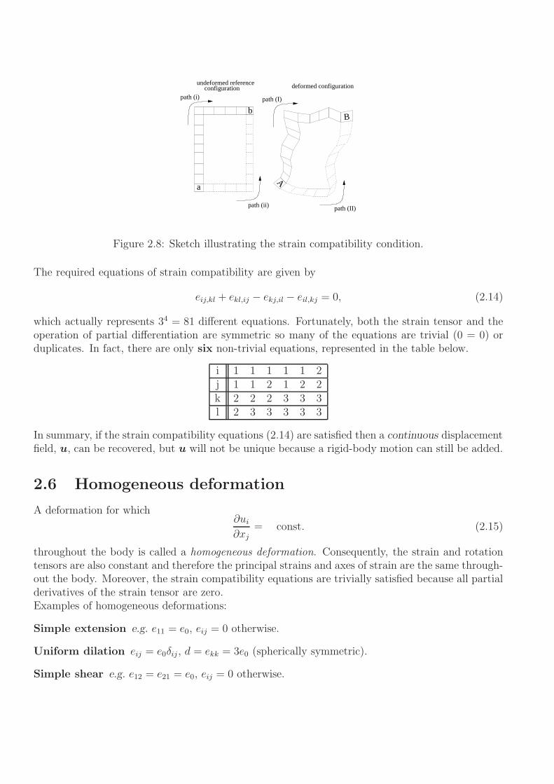
configuration

a

b

A

path (i)

deformed configuration

path (I)

path (II)path (ii)

B

undeformed reference

Figure 2.8: Sketch illustrating the strain compatibility condition.

The required equations of strain compatibility are given by

eij,kl + ekl,ij − ekj,il − eil,kj = 0, (2.14)

which actually represents 34 = 81 different equations. Fortunately, both the strain tensor and theoperation of partial differentiation are symmetric so many of the equations are trivial (0 = 0) orduplicates. In fact, there are only six non-trivial equations, represented in the table below.

i 1 1 1 1 1 2j 1 1 2 1 2 2k 2 2 2 3 3 3l 2 3 3 3 3 3

In summary, if the strain compatibility equations (2.14) are satisfied then a continuous displacementfield, u, can be recovered, but u will not be unique because a rigid-body motion can still be added.

2.6 Homogeneous deformation

A deformation for which∂ui

∂xj= const. (2.15)

throughout the body is called a homogeneous deformation. Consequently, the strain and rotationtensors are also constant and therefore the principal strains and axes of strain are the same through-out the body. Moreover, the strain compatibility equations are trivially satisfied because all partialderivatives of the strain tensor are zero.Examples of homogeneous deformations:

Simple extension e.g. e11 = e0, eij = 0 otherwise.

Uniform dilation eij = e0δij , d = ekk = 3e0 (spherically symmetric).

Simple shear e.g. e12 = e21 = e0, eij = 0 otherwise.

Chapter 3

Analysis of stress

Lecture 7

3.1 Introductory concepts

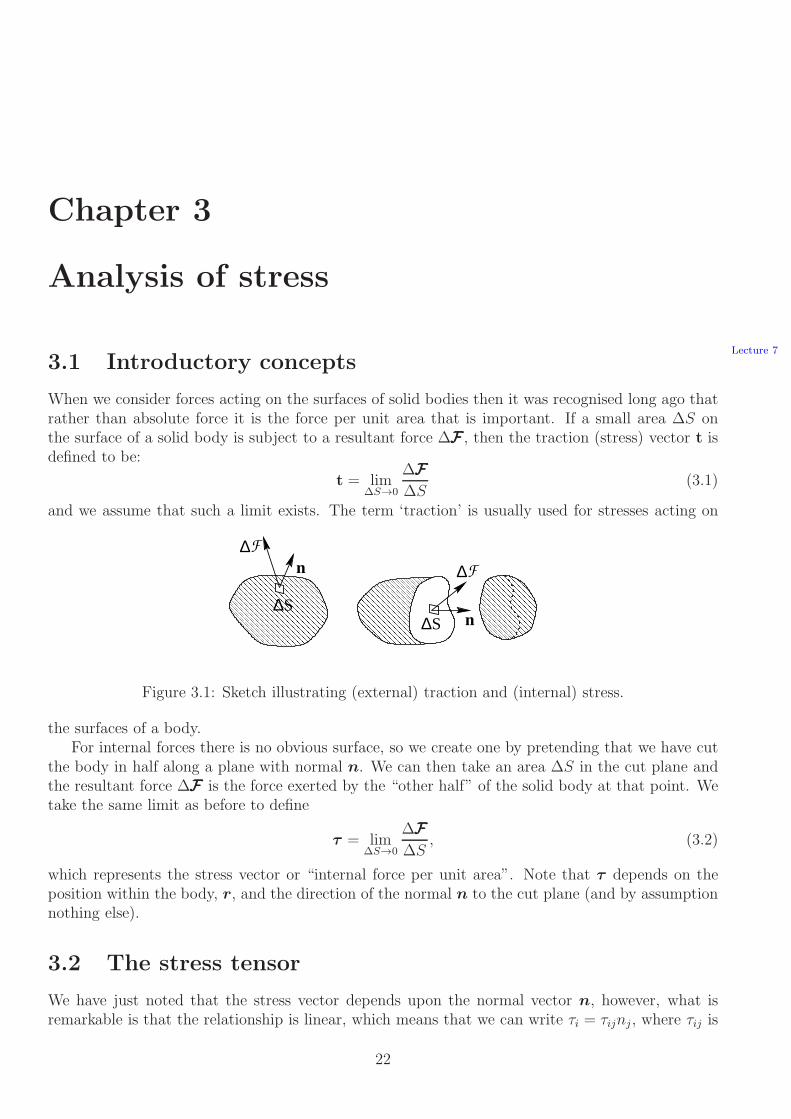
When we consider forces acting on the surfaces of solid bodies then it was recognised long ago thatrather than absolute force it is the force per unit area that is important. If a small area ∆S onthe surface of a solid body is subject to a resultant force ∆FFF , then the traction (stress) vector t isdefined to be:

t = lim∆S→0

∆FFF∆S

(3.1)

and we assume that such a limit exists. The term ‘traction’ is usually used for stresses acting on

��

��

��

��

��

��

∆F

S

n

∆ S∆

∆F

n

Figure 3.1: Sketch illustrating (external) traction and (internal) stress.

the surfaces of a body.For internal forces there is no obvious surface, so we create one by pretending that we have cut

the body in half along a plane with normal n. We can then take an area ∆S in the cut plane andthe resultant force ∆FFF is the force exerted by the “other half” of the solid body at that point. Wetake the same limit as before to define

τ = lim∆S→0

∆FFF∆S

, (3.2)

which represents the stress vector or “internal force per unit area”. Note that τ depends on theposition within the body, r, and the direction of the normal n to the cut plane (and by assumptionnothing else).

3.2 The stress tensor

We have just noted that the stress vector depends upon the normal vector n, however, what isremarkable is that the relationship is linear, which means that we can write τi = τijnj , where τij is

22

called the stress tensor. In order to prove this we must consider the balance of forces within a smalltetrahedral region, see Figure 3.2. Three of the tetrahedron’s faces are in the planes xi is constant

x2

τ 1

τn

e1

x1

x3

Figure 3.2: A tetrahedron is formed between Cartesian coordinate axes. The coordinate xi is aconstant on face i, which has outer unit normal ei. The resultant stress vector acting on the i-thface is τ i.

and these have area dSi and outer unit normal ei. Thus we can represent these faces by a singlevector with orientation ei and magnitude equal to dSi. The final face does not lie in any coordinateplane and has normal n and area dS. It follows from vector geometry that

eidSi + ndS = 0, (exercise). (3.3)

Taking the dot product of equation (3.3) with ej gives

ej·eidSi + ej·ndS = 0,

and if we let n = (n1, n2, n3) in the Cartesian basis then

δijdSi + njdS = 0 ⇒ dSj = −njdS. (3.4)

We now assume that the resultant stress acting on the face on which xi is constant is τ i and theresultant stress on the remaining face is τ . If the tetrahedron is in equilibrium then the totalresultant force, the sum of the forces acting on all the faces, must be zero, i.e.,

τdS + τ jdSj = 0,

where we have used the fact that force is stress multiplied by area (a bit of careful thought showsthat for small tetrahedra body forces are negligible because the volume [cube of a small length] ismuch smaller than the the surface area [square of small length]). Thus,

τdS = −τ jdSj = τ jnjdS,

after using equation (3.4). This demonstrates the required linear relationship between τ and n andhence we must be able to write out in components

τi = τijnj ,

as claimed above, where τij is called the stress tensor. The component τij represents the i-thcomponent of the stress on the face whose outer unit normal points in the xj direction, see Figure3.3. Note that the components on opposite faces point in opposite directions because the sign of

��

��

��

��

��

��

��

��

��

��

��

��τ

x x

x

1 2

3

τ 11τ

τ 31

21 ττ

τ12 22

32

ττ 23

33

13

τ

3

31

τ11τ 21

τ 33

τ 23 13τ

τ 22

τ32

τ 12

x x

x

1 2

Figure 3.3: Sketch illustrating the components of the stress tensor.

the normal is reversed.We can now represent the internal stress state of the body in terms of the stress tensor, but it

remains to determine τij as a function of the state of strain.

3.3 Equilibrium of forces

Consider an infinitesimal region of our elastic body that is loaded by an internal traction τ on itssurface and a body force F per unit volume. Hence, if the body is to be in equilibrium the totalforce must be zero: ∫∫

S

τ dS +

∫∫∫

V

F dV = 0.

The above expression represents the sum of the surface (stress) and volume (body) forces. Incomponent form, we can write

∫∫

S

τi dS +

∫∫∫

V

Fi dV =

∫∫τijnj dS +

∫∫∫

V

Fi dV = 0.

The surface integral can be converted into a volume integral by means of the divergence theorem,∫∫∫

V

(τij,j + Fi) dV = 0.

The above integral must be zero for all possible volumes and so (assuming suitable existence andsmoothness), we must have that

τij,j + Fi = 0 ⇒ ∂τij∂xj

+ Fi = 0, (3.5)

which are the equations of equilibrium.This equation can be generalised to the unsteady case via Newton’s second law or, equivalently,

D’Alembert’s principle and we obtain the equations of motion

ρui = τij,j + Fi, (3.6)

where ρ is the density of the solid and u = ∂2u∂t2

is the acceleration. These are sometimes calledCauchy’s equations and are Newton’s second law, ma = F , generalised to an elastic solid.

3.4 Symmetry of the stress tensor and principal axes/stress

invariants

The stress tensor is symmetric (τij = τji) which can be proved by considering a moment (force ×distance) balance about all axes parallel to ei through the centre of the block. Consequently, thediscussion in section 2.4 applies to the stress tensor as well. Thus, the stress tensor has principalstresses, principal axes of stress and three invariants. In particular, we will denote the first invariant(the trace of the stress tensor) by

Θ = τii. (3.7)

Lecture 8

3.5 Homogeneous stress states

These states are analogous to homogeneous deformations (see section 2.6): Examples of homoge-neous stress states:

Uniaxial stress e.g. τ33 = T0, τij = 0 otherwise.

Hydrostatic pressure τij = −pδij (spherically symmetric).

Simple shear stress e.g. τ12 = τ21 = T0, τij = 0 otherwise.

3.6 Stress boundary conditions

There must be “continuity of stress” at all boundaries. Thus, if there is a given applied traction t

at the surface of the elastic body, it must equal the internal stress at the surface:

τ = t ⇒ τi = ti ⇒ τijnj = ti

where n is now the outer unit normal to the body.

Example

Consider a unit square loaded only by an external pressure, p0 (no body forces), see Figure 3.4.Pressure is always directed normally into the body. Thus, for any face, a pressure load is t = −p0nif n is the outer unit normal.

x1

x2

n1 = e1

n2 = e2

Face 1

Face 2

Face 3

Face 4Figure 3.4: A unit square is loaded only by an external pressure p0.

On Face 1, the load is t = −p0e1 = −p0n1. Thus, t1 = −p0 and t2 = 0 because n = (1, 0).From continuity of stress τijnj = ti, so putting i = 1 and expanding the sum yields

τ11n1 + τ12n2 = t1 = −p0 ⇒ τ11 = −p0.

Note that τ11 represents the stress component in the positive x1 direction. Hence it is negative inthis case because the body is compressed: the traction (pressure) acts into the body. Repeating thesame procedure for i = 2 we obtain

τ21n1 + τ22n2 = t2 = 0 ⇒ τ21 = τ12 = 0.

Note that we do not get boundary conditions for all components of the stress tensor!On Face 2, the load is t = −p0e2 = −p0n2. Thus, t1 = 0 and t2 = −p0 because n2 = (0, 1).

From continuity of stress we have

i = 1 : τ11n1 + τ12n2 = τ12 = τ21 = 0,

i = 2 : τ21n1 + τ22n2 = τ22 = −p0.

Similar expressions could be found for Faces 3 and 4 and if the stress tensor takes the form τij =−p0δij it satisfies the stress boundary conditions on all of the square’s faces and we see that a purepressure loading yields a hydrostatic pressure stress tensor. Note that this trivially satisfies theequations of equilibrium because it is a constant.

3.7 Resultant force and moments

For a given traction distribution, t, at the surface of a body, the resultant force is the integral ofthe traction over the body’s surface:

F =

∫∫

S

t dS or Fi =

∫∫

S

τijnj dS,

and the resultant moment about a given point is

M =

∫∫

S

r × t dS,

where r is the vector distance from the point being considered to a point on the surface and × isthe usual vector cross product. For a body to be in equilibrium, the resultant force and resultantmoment about any point must be zero (or must balance the body forces if present).

Example

Let us return to the example of the unit square loaded by an external pressure considered above.We can calculate the resultant force applied to the square by summing the forces on each of the fourfaces. On Face 1, t = −p0e1, on Face 2, t = −p0e2, on Face 3, t = p0e1 and on Face 4, t = p0e2;therefore, if we set the origin to be the bottom left corner of the square, the resultant force is

F =∫ y=1

y=0(−p0e1)dy +

∫ x=1

x=0(−p0e2)dx +

∫ y=1

y=0(p0e1)dy +

∫ x=1

x=0(p0e2)dx = 0.

Face 1 Face 2 Face 3 Face 4

If we consider the resultant moment about the origin, then on Face 1, r = e1 + ye2, on Face 2,r = xe1 + e2, on Face 3, r = ye2 and on Face 4, r = xe1 and therefore,

M =

∫ y=1

y=0

(e1 + ye2)× (−p0e1)dy +

∫ x=1

x=0

(xe1 + e2)× (−p0e2)dx+

∫ y=1

y=0

(ye2)× (p0e1)dy

+

∫ x=1

x=0

(xe1)× (p0e2)dx

=

∫ y=1

y=0

(p0ye3)dy +

∫ x=1

x=0

(−p0xe3)dx+

∫ y=1

y=0

(−p0ye3)dy +

∫ x=1

x=0

(p0xe3)dx = 0.

The resultant force and moment are both zero and the body is in equilibrium.

Chapter 4

Elasticity & constitutive equations

Lecture 9

4.1 The constitutive equations

Thus far we have characterized deformation by strains (see chapter 2) and internal forces by stresses(see chapter 3), from which we could deduce equations of motion. We now ask the obvious question:

How do the stresses relate to the strains?

The relationship between stresses and strains is called the constitutive law and characterises thebehaviour of the material under consideration.

In a general elastic body, the stresses are functions only of the instantaneous, local strains:

τij(r, t) = τij(ekl(r, t)), (4.1)

and each of the six independent components of the stress tensor can depend on all six independentcomponents of the strain tensor.

For small strains, a Taylor expansion of (4.1) gives

τij = τij |ekl=0︸︷︷︸Initial Stress τ

(0)ij

+∂τij∂ekl

∣∣∣∣ekl=0︸︷︷︸

Eijkl

ekl, (4.2)

which motivates the definition that a solid is linearly elastic if:

τij = τ(0)ij + Eijklekl. (4.3)

If the initial stress in the undeformed configuration is zero, then we obtain Hooke’s law:

τij = Eijklekl. (4.4)

Most solids are linearly elastic for sufficiently small strains.The 4-th rank tensor Eijkl has 3

4 = 81 coefficients, but because both eij and τij are symmetricthe coefficients of Eijkl are not all independent. In fact, there are only 21 independent coefficients,but these must be determined from experiments.

Definition: A solid body is called homogeneous if Eijkl is independent of xi.

Definition: A solid body is called isotropic if its elastic properties are the same in all directions(i.e. there are no reinforcing fibres or other “directed” internal structures).

28

For an isotropic, homogeneous, elastic solid there are only two independent coefficients thatmust be determined experimentally and

Eijkl = λδijδkl + 2µδikδjl. (4.5)

Here, λ and µ are the independent coefficients known as the Lame constants.Hence, the constitutive law for an isotropic, homogeneous, linearly elastic solid is

τij = Eijklekl = (λδijδkl + 2µδikδjl) ekl,

⇒ τij = λδij ekk︸︷︷︸=d

+2µeij. (4.6)

Note that the principal axes of eij and τij coincide (exercise). Also if there is no volume changethen d = 0 and τij is linearly proportional to eij .

Inverse form

Equation (4.6) gives an explicit expression for the stress in terms of the strain, but what is thestrain for a given stress? If d = 0, the answer is simple, but in general we need to work a littleharder. Firstly, set i = j in equation (4.6)

τii = 3λekk + 2µeii = (3λ+ 2µ) d ⇒ Θ = (3λ+ 2µ) d,

where Θ = τii and d = eii. Rearranging (4.6) gives

eij =1

2µ(τij − λδijd) ,

⇒ eij =1

2µ

(τij − λδij

Θ

3λ+ 2µ

).

Thus,

eij =1

2µτij −

λ

2µ (3λ+ 2µ)δijτkk,

which can be written aseij = Dijklτkl, (4.7)

where

Dijkl =1

2µδikδjl −

λ

2µ (3λ+ 2µ)δijδkl.

Rest ofchapter isreadingweek ma-terial andnot coveredexplicitly inlectures

4.2 Experimental determination of elastic constants

4.2.1 Experiment I: Simple extension of a thin cylinder

A circular cylinder of diameter D, cross-sectional area A and initial length L is subject to an appliedtension T along its axis which is chosen to lie in the x3 direction. After the load has been appliedthe cylinder has length L+∆L and diameter D +∆D.

The extension is in the x3 direction and so e33 = ∆L/L ≪ 1. The change in diameter is in thex1 and x2 directions, so e11 = e22 = ∆D/D. Moreover, the stress is uniaxial (along one axis, x3) soτ33 = T/A, and τij = 0 otherwise.

L+ L ∆

x3 ��

∆ D+ DD

T

T

L

I. Simple Extension

τ

γ

II. Simple Shear

x

x1

2

Figure 4.1: Sketch illustrating the two fundamental experiments for the determination of the elasticconstants.

• Observations:

– Rod extends in the x3 direction in proportion to the applied tension:

τ33 = Ee33, where E is the Elastic (or Young’s) modulus. (4.8)

– Rod cross-section decreases (contracts in plane) in proportion to its extension in the axialdirection:

e11 = e22 = −ν e33, where ν is the Poisson ratio. (4.9)

4.2.2 Experiment II: Simple shear

A block in the x1-x2 plane is subject to an applied traction, τ , on its upper surface in the positivex1 direction that induces a change in angle γ = 2e12 between two sides. The body is in a state ofsimple shear so τ12 = τ and τij = 0 otherwise.

• Observation:

– The change in angle is proportional to the applied traction:

τ = Gγ ⇒ τ12 = G 2e12, where G is the shear modulus of the material. (4.10)

4.3 Relating experiments (E, ν,G) and theory (λ, µ)

We shall now use the constitutive equations to relate the experimentally measured constants E, νand G to the (theoretical) Lame coefficients λ and µ. The material is homogeneous, isotropic andelastic so that

τij = λδijekk + 2µ eij, (4.11)

and, alternatively,

eij =1

2µτij −

λ

2µ(3λ+ 2µ)δijτkk. (4.12)

Experiment I

In this experiment, τ33 = Ee33 and Θ = τkk = τ33, because τ11 = τ22 = 0. If we set i = j = 3 inequation (4.12) we have

e33 =1

2µτ33 −

λ

2µ(3λ+ 2µ)τkk =

[1

2µ− λ

2µ(3λ+ 2µ)

]τ33 =

[3λ+ 2µ− λ

2µ(3λ+ 2µ)

]τ33 =

λ+ µ

µ(3λ+ 2µ)τ33.

Hence,1

E=

λ+ µ

µ(3λ+ 2µ)⇒ E = µ(3λ+2µ)

λ+µ. (4.13)

If we substitute i = j = 1 into equation (4.12), we obtain

e11 =1

2µτ11 −

λ

2µ(3λ+ 2µ)τ33 = − λ

2µ(3λ+ 2µ)τ33, because τ11 = 0.

Using the first experimental observation, τ33 = Ee33, and the expression (4.13) for E gives

e11 = − λ

2µ(3λ+ 2µ)

µ(3λ+ 2µ)

λ+ µe33 = − λ

2(λ + µ)e33.

The second experimental observation is e11 = −ν e33, so direct comparison yields

ν = λ2(λ+µ)

. (4.14)

Note that an identical result is obtained on substitution of i = j = 2 into equation (4.12).

Experiment II

In this experiment, τ12 = 2Ge12, and using equation (4.11) with i = 1 and j = 2, we have

τ12 = λδ12ekk + 2µ e12 = 2µ e12 ⇒ µ = G. (4.15)

4.4 Relations between the elastic constants

Note that only two elastic constants are independent, see equations (4.11, 4.12). The following tablelists the relationships between elastic coefficients for the most commonly used independent pairs.

Independent pair λ = µ = G = E = ν =

λ, µ λ µ µ(3λ+2µ)λ+µ

λ2(λ+µ)

λ, ν λ λ(1−2ν)2ν

(1+ν)(1−2ν)λν ν

µ, E µ(E−2µ)3µ−E

µ E E−2µ2µ

E, ν Eν(1+ν)(1−2ν)

E2(1+ν) E ν

4.4.1 Constitutive equations in terms of the experimentally measurable

constants

Using the table above, we can rewrite the equation (4.11) and (4.12) using the Young’s modulus Eand Poisson ratio ν

τij =E

1 + ν

eij +

ν

1− 2νδij ekk︸︷︷︸

d

. (4.16)

and

eij =1

E

(1 + ν)τij − ν δij τkk︸︷︷︸

Θ

. (4.17)

For physically realisable materials,

E ≥ 0, −1 < ν ≤ 1

2, µ ≥ 0, 3λ+ 2µ > 0.

Note that equation (4.17) implies that

d = ekk =τkkE

((1 + ν)− 3ν) =Θ

E(1− 2ν) ,

and so d = 0, when ν = 1/2. Materials for which ν = 1/2 are thus said to be incompressible. Caremust be taken when considering the limit ν → 1/2 in equation (4.16). In fact, the limit in questionis ν → 1/2 and d → 0, in such a way that the term d/(1− 2ν) remains finite.

Chapter 5

The governing equations of linearelasticity

Lecture 10

5.1 Navier–Lame equations — displacement formulation

In the previous chapters we have established the following equations:

Definition of strain eij =12(ui,j + uj,i), (5.1a)

Equations of motion τij,j + Fi = ρ∂2ui

∂t2, (5.1b)

Linear elastic constitutive law τij = λδijekk + 2µeij (5.1c)

The idea is to eliminate the stress and strain to obtain an equation that only contains the displace-ment u. Using equation (5.1a) in equation (5.1c) we obtain an expression for the stresses in termsof the displacements

τij = λ δij uk,k + µ (ui,j + uj,i) . (5.2)

Now, taking the derivative of equation (5.2) gives

τij,j = λ δij uk,kj + µ (ui,jj + uj,ij) = λ uk,ki + µ ui,jj + µuj,ji = (λ+ µ)uk,ki + µ ui,jj,

by using the symmetry of the partial derivative and the index-switching property of the Kroneckerdelta. Using the last result in equation (5.1b), we obtain the Navier–Lame equations

ρui = (λ + µ) uk,ki + µui,jj + Fi. (5.3)

The Navier–Lame equations may be written in the equivalent form

ρu = (λ+ µ) grad(divu) + µ∇2u+ F ,

or evenρu = (λ+ 2µ) grad(divu)− µ curl(curlu) + F ,

by using the vector identity∇2u = grad(divu)− curl(curlu).

However they are written, these Navier–Lame equations are a system of three coupled linear PDEsfor the three displacements ui(xj).

33

Note

• The general case of a non-zero body force is not very different from the “special” case F = 0because the Navier–Lame equations are linear. F acts as an inhomogeneity that can beremoved if a suitable particular solution is found. We seek a function u such that

(λ+ µ)∇∇ · u+ µ∇2u+ F − ρ¨u = 0,

irrespective of the boundary conditions. If we then define the displacement field to be u =u+ u, then u satisfies the homogeneous equation

(λ+ µ)∇∇ · u+ µ∇2u− ρ¨u = 0,

but the boundary conditions may have changed from the original problem.

5.2 Boundary conditions for the Navier–Lame equations:

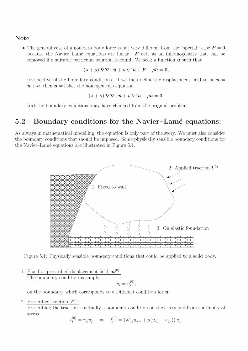
As always in mathematical modelling, the equation is only part of the story. We must also considerthe boundary conditions that should be imposed. Some physically sensible boundary conditions forthe Navier–Lame equations are illustrated in Figure 5.1.

1: Fixed to wall

2: Applied traction t(0)

3: On elastic foundation

Figure 5.1: Physically sensible boundary conditions that could be applied to a solid body.

1. Fixed or prescribed displacement field, u(0).The boundary condition is simply

ui = u(0)i ,

on the boundary, which corresponds to a Dirichlet condition for u.

2. Prescribed traction, t(0).Prescribing the traction is actually a boundary condition on the stress and from continuity ofstress

t(0)i = τijnj ⇒ t

(0)i = (λδijuk,k + µ(ui,j + uj,i))nj,

from the constitutive law. The resulting equation is a condition on the derivatives of u at theboundary, which is a Neumann boundary condition.

3. Elastic bedding.In this case the applied traction is related to the displacement of the boundary. Consider thesimplified problem in which there is a single linear spring connected to our elastic body thatcan move only in the x1 direction, see Figure 5.2.

✲

✻

x1

x2

t(0)✲✛ l

✲✛ l + u1

T = k1u1

t(0)

Figure 5.2: An elastic body is attached by spring of undeformed length l to a solid wall. Theelastic body is subject to the external traction t(0) in the positive x1 direction (upper image). Afterapplication of the traction, the spring extended to the length l + u1, where u1 is the displacementof the solid body in the x1 direction (lower image). For a linear spring, the tension (restoring force)is T = k1u1 which acts in the negative x1 direction.

If we assume that the spring is in its rest state when u1 = 0 then the tension in the spring isT = k1u1, where k1 is the spring constant and it acts in the negative x1 direction. Resolvingforces in the x1 direction gives

t(0)1︸︷︷︸

Applied traction

− k1u1︸︷︷︸Restoring force

= τ1jnj = −τ11︸︷︷︸stress at surface

.

Thus, the surface stress is related to the displacement through the restoring force applied bythe spring.

For a general (linear) elastic foundation

t(0)i = τijnj + kijuj,

where kij is a stiffness tensor (or matrix of spring coefficients). This type of boundary conditionis a mixed or Robin condition.

Whatever boundary conditions are applied, once we have solved the Navier–Lame equations (5.3) tofind the displacement field u, we can use equations (5.1a) and (5.1c) to determine the correspondingstrain and stress fields.

5.3 Beltrami–Michell equations — stress formulationRemainderof chapteris readingweek ma-terial andnot coveredexplicitly inlectures

The Navier–Lame equations treat the displacements as the unknowns in elasticity problems; thestrains and stresses are calculated indirectly, once the displacements are known. An alternative

approach is to formulate the set of governing equations so that the stresses are the unknowns andare calculated directly. We can then use the constitutive law to determine the strains and hencethe displacements. There is a potential problem, however – the displacements cannot be uniquelyrecovered from the strain field unless the strain compatibility conditions are satisfied.

eij,kl + ekl,ij − ekj,il − eil,kj = 0. (5.4)

The inverse form of the linear constitutive law (5.1c) is

eij =1

2µτij −

λ

2µ(3λ+ 2µ)δijτkk,

and using the engineering (experimental) constants E and ν, we obtain a slightly neater expression

E

1 + νeij = τij −

ν

1 + νδijΘ. (5.5)

Substituting the expression (5.5) into the strain compatibility equations (5.4) yields

τij,kl + τkl,ij − τkj,il − τil,kj −ν

1 + ν

[δijΘ,kl + δklΘ,ij − δkjΘ,il − δilΘ,kj

]= 0.

All the terms in the above expression are second derivatives of τij , so that the equations are allsatisfied if the stress is a linear function of position, in which case every term is zero. Rememberthat only six of these 81 equations are linearly independent, so we are free to combine equations bysetting k = l and summing over the repeated index to obtain nine equations, of which six are stillindependent through the symmetry of the stress tensor,

τij,kk + τkk,ij − τkj,ik − τik,kj −ν

1 + ν[δijΘ,kk + δkkΘ,ij − δkjΘ,ik − δikΘ,kj] = 0.

Using the fact that τkk = Θ, δkk = 3 and the index-switching property of the Kronecker delta, theequations become

τij,kk +Θ,ij − τkj,ik − τik,kj −ν

1 + ν[δijΘ,kk + 3Θ,ij −Θ,ij −Θ,ij] = 0,

⇒ τij,kk +Θ,ij − τkj,ik − τik,kj −ν

1 + ν[δijΘ,kk +Θ,ij] = 0,

⇒ τij,kk +1

1 + νΘ,ij −

ν

1 + νΘ,kkδij − τkj,ik − τik,kj = 0. (5.6)

The equation (5.6) can be written in the alternative form

∇2τij +1

1 + νΘ,ij −

ν

1 + νδij∇2Θ = τkj,ik + τik,kj. (5.7)

Differentiating the equations of static equilibrium τij,j + Fi = 0, we obtain τij,jk + Fi,k = 0, whichcan be used to replace the terms on the right-hand side of equation (5.7).

∇2τij +1

1 + νΘ,ij −

ν

1 + νδij∇2Θ = −Fj,i − Fi,j . (5.8)

Setting i = j in equation (5.8) gives

∇2τii +1

1 + νΘ,ii −

ν

1 + ν3∇2Θ = −2Fi,i ⇒ ∇2Θ+

1

1 + ν∇2Θ− 3ν

1 + ν∇2Θ = −2Fi,i

⇒ 1− ν

1 + ν∇2Θ = −Fi,i; (5.9)

and on substitution of (5.9) into equation (5.8) we finally obtain the Beltrami–Michell (compatibil-ity) equations

∇2τij +1

1+ν Θ,ij +ν

1−ν δijFk,k + Fi,j + Fj,i = 0. (5.10)

These are stress compatibility equations and we note that in unsteady problems, we must add theinertia force −ρui to Fi.

The Beltrami–Michell equations are six linear partial PDEs for the six independent componentsof the stress tensor. As one might expect, these equations are (very) useful if the problem hasstress boundary conditions. The equations are less useful if displacement boundary conditions arespecified.

Notes

• The equations of equilibrium are automatically satisfied by construction.

• The strains eij can be recovered from the constitutive equation.

• Once the strain field is known, the displacements can be obtained by integrating

eij =1

2(ui,j + uj,i) .

Remember that the constants of integration represent rigid-body motions.

• The above integration is possible because we started from the strain compatibility equationsand, therefore, if the Beltrami–Michell equations are satisfied, so are the strain compatibilityequations; and hence, the body will be continuous.

5.4 The steady, constant-body-force case

If the body force is a constant and there are no unsteady terms, then all of the derivatives Fi,j willbe zero. The Beltrami–Michell equations become

∇2τij +1

1 + νΘ,ij = 0,

and from equation (5.9) we have∇2Θ = 0.

Thus, Θ is a harmonic function: a function that satisfies Laplace’s equation. Recall that Θ =(3λ+ 2µ) d, which implies that

∇2d = 0,

and so d = ekk = uk,k is also a harmonic function. If we apply the operator ∇2 to the (steady)Navier–Lame equations (5.3) we obtain

(λ+ µ) uk,kijj + µ ui,kkjj = 0.

The first term may be written as (uk,kjj),i and because uk,k is harmonic then uk,kjj = 0 and hencethe first term is zero. Thus,

ui,kkjj = 0, or rather ∇4 u = 0,

and so the displacement field is a solution of the biharmonic equation. Furthermore, by usingthe definition of the strain tensor (5.1a) and the expression for the stress tensor in terms of thedisplacements (5.2), it follows that

∇4 τij = 0, and ∇4 eij = 0;

the stress and strain components are both biharmonic functions.

5.5 Alternative coordinate systems:

5.5.1 Governing Equations in Cylindrical Polar Coordinates

• x1 = x = r cos θ, x2 = y = r sin θ, x3 = z = z.

u = (ur, uθ, uz), E = (eij), τ = (τij), where i, j = r, θ, z.

• Vector calculus:

grad f =∂f

∂rr+

1

r

∂f

∂θθ +

∂f

∂zz, divu =

1

r

∂(rur)

∂r+

1

r

∂uθ

∂θ+

∂uz

∂z,

curlu =

(1

r

∂uz

∂θ− ∂uθ

∂z

)r+

(∂ur

∂z− ∂uz

∂r

)θ +

(1

r

∂(ruθ)

∂r− 1

r

∂ur

∂θ

)z.

• Stress-strain relations have the same form as in Cartesian coordinates:

τij = λδij divu+ 2µeij, i, j = r, θ, z.

• Stress-displacement relations:

τrr = λ divu+ 2µ∂ur

∂r, τθθ = λ divu+ 2µ

(1

r

∂uθ

∂θ+

ur

r

), τzz = λ divu+ 2µ

∂uz

∂z,

τrθµ

=τθrµ

=∂uθ

∂r− uθ

r+

1

r

∂ur

∂θ,

τrzµ

=τzrµ

=∂uz

∂r+

∂ur

∂z,

τθzµ

=τzθµ

=1

r

∂uz

∂θ+

∂uθ

∂z.

• Strain-displacement relations:

err =∂ur

∂r, eθθ =

1

r

∂uθ

∂θ+

ur

r, ezz =

∂uz

∂z,

2erθ = 2eθr =∂uθ

∂r− uθ

r+

1

r

∂ur

∂θ, 2erz = 2ezr =

∂ur

∂z+

∂uz

∂r, 2ezθ = 2eθz =

1

r

∂uz

∂θ+

∂uθ

∂z.

• Equilibrium equations (statics): for the displacement formulation, use Navier’s equation,

(λ+ 2µ) grad divu− µ curl curlu+ F = 0,

whereas for the stress formulation, use

∂τrr∂r

+1

r

∂τrθ∂θ

+∂τrz∂z

+τrr − τθθ

r+ Fr = 0

∂τrθ∂r

+1

r

∂τθθ∂θ

+∂τθz∂z

+2

rτrθ + Fθ = 0

∂τrz∂r

+1

r

∂τθz∂θ

+∂τzz∂z

+1

rτrz + Fz = 0.

• Stress boundary conditions: these are when t is prescribed. We have, from ti = njτij,

tr = nrτrr + nθτrθ + nzτrz

tθ = nrτrθ + nθτθθ + nzτθz

tz = nrτrz + nθτθz + nzτzz.

5.5.2 Governing Equations in Spherical Polar Coordinates

• x1 = x = r sin θ cosφ, x2 = y = r sin θ sinφ, x3 = z = r cos θ. Note: θ is the polar angle andφ is the azimuthal angle.

u = (ur, uθ, uφ), E = (eij), τ = (τij), where i, j = r, θ, φ.

• Vector calculus:

grad f =∂f

∂rr+

1

r

∂f

∂θθ +

1

r sin θ

∂f

∂φφ,

divu =1

r2 sin θ

{∂

∂r(r2 sin θ ur) +

∂

∂θ(r sin θ uθ) +

∂

∂φ(ruφ)

},

curlu =1

r2 sin θ

∣∣∣∣∣∣

r rθ r sin θ φ∂∂r

∂∂θ

∂∂φ

ur ruθ r sin θ uφ

∣∣∣∣∣∣.

• Stress-strain relations have the same form as in Cartesian coordinates:

τij = λδij divu+ 2µeij , i, j = r, θ, φ.

• Stress-displacement relations:

τrr = λ divu+ 2µ∂ur

∂r, τθθ = λ divu+

2µ

r

(∂uθ

∂θ+ ur

),

τφφ = λ divu+2µ

r

(1

sin θ

∂uφ

∂φ+ ur + uθ cot θ

),

τrθµ

=τθrµ

=∂uθ

∂r− uθ

r+

1

r

∂ur

∂θ,

τrφµ

=τφrµ

=1

r sin θ

∂ur

∂φ+

∂uφ

∂r− uφ

r,

τθφµ

=τφθµ

=1

r sin θ

∂uθ

∂φ+

1

r

∂uφ

∂θ− uφ cot θ

r.

• Strain-displacement relations:

err =∂ur

∂r, eθθ =

1

r

∂uθ

∂θ+

ur

r, eφφ =

1

r sin θ

∂uφ

∂φ+

ur

r+

uθ cot θ

r,

2erθ = 2eθr =∂uθ

∂r− uθ

r+

1

r

∂ur

∂θ, 2erφ = 2eφr =

1

r sin θ

∂ur

∂φ+

∂uφ

∂r− uφ

r,

2eφθ = 2eθφ =1

r sin θ

∂uθ

∂φ+

1

r

∂uφ

∂θ− uφ cot θ

r.

• Equilibrium equations (statics): for the displacement formulation, use Navier’s equation,

(λ+ 2µ) grad divu− µ curl curlu+ F = 0,

whereas for the stress formulation, use

∂τrr∂r

+1

r

∂τrθ∂θ

+1

r sin θ

∂τrφ∂φ

+2τrr − τθθ − τφφ + cot θ τrθ

r+ Fr = 0

∂τrθ∂r

+1

r

∂τθθ∂θ

+1

r sin θ

∂τθφ∂φ

+3τrθ + (τθθ − τφφ) cot θ

r+ Fθ = 0

∂τrφ∂r

+1

r

∂τθφ∂θ

+1

r sin θ

∂τφφ∂φ

+3τrφ + 2τθφ cot θ

r+ Fφ = 0.

• Stress boundary conditions: these are when t is prescribed. We have, from ti = njτij,

tr = nrτrr + nθτrθ + nφτrφ

tθ = nrτrθ + nθτθθ + nφτθφ

tφ = nrτrφ + nθτθφ + nφτφφ.

Chapter 6

Problems with variation in only onedirection (1D)

Lecture 11

6.1 Infinite cylindrical pipe under internal pressure

An infinite cylindrical pipe is loaded by an internal pressure p0, see Figure 6.1, and has inner radiusa and outer radius b.

xxxxxxxxxxxxxxxxxxxxxxxxxxxxxxxxxxxxxxxxxxxxxxxxxxxxxxxxxxxxxxxxxxxxxxxxxxxxxxxxxxxxxxxxxxxxxxxxxxxxxxxxxxxxxxxxxxxxxxxxxxxxxxxxxxxxxxxxxxxxxxxxxxxxxxxxxxxxxxxxxxxxxxxxxxxxxxxxxxxxxxxxxxxxxxxxxxxxxxxxxxxxxxxxxxxxxxxxxxxxxxxxxxxxxxxxxxxxxxxxxxxxxxxxxxxxxxxxxxxxxxxxxxxxxxxxxxxxxxxxxxxxxxxxxxxxxxxxxxxxxxxxxxxxxxxxxxxxxxxxxxxxxxxxxxxxxxxxxxxxxxxxxxxxxxxxxxxxxxxxxxxxxxxxxxxxxxxxxxxxxxxxxxxxxxxxxxxxxxxxxxxxxxxxxxxxxxxxxxxxxxxxxxxxxxxxxxxxxxxxxxxxxxxxxxxxxxxxxxxxxxxxxxxxxxxxxxxxxxxxxxxxxxxxxxxxxxxxxxxxxxxxxxxxxxxxxxxxxxxxxxxxxxxxxxxxxxxxxxxxxxxxxxxxxxxxxxxxxxxxxxxxxxxxxxxxxxxxxxxxxxxxxxxxxxxxxxxxxxxxxxxxxxxxxxxxxxxxxxxxxxxxxxxxxxxxxxxxxxxxxxxxxxxxxxxxxxxxxxxxxxxxxxxxxxxxxxxxxxxxxxxxxxxxxxxxxxxxxxxxxxxxxxxxxxxxxxxxxxxxxxxxxxxxxxxxxxxxxxxxxxxxxxxxxxxxxxxxxxxxxxxxxxxxxxxxxxxxxxxxxxxxxxxxxxxxxxxxxxxxxxxxxxxxxxxxxxxxxxxxxxxxxxxxxxxxxxxxxxxxxxxxxxxxxxxxxxxxxxxxxxxxxxxxxxxxxxxxxxxxxxxxxxxxxxxxxxxxxxxxxxxxxxxxxxxxxxxxxxxxxxxxxxxxxxxxxxxxxxxxxxxxxxxxxxxxxxxxxxxxxxxxxxxxxxxxxxxxxxxxxxxxxxxxxxxxxxxxxxxxxxxxxxxxxxxxxxxxxxxxxxxxxxxxxxxxxxxxxxxxxxxxxxxxxxxxxxxxxxxxxxxxxxxxxxxxxxxxxxxxxxxxxxxxxxxxxxxxxxxxxxxxxxxxxxxxxxxxxxxxxxxxxxxxxxxxxxxxxxxxxxxxxxxxxxxxxxxxxxxxxxxxxxxxxxxxxxxxxxxxxxxxxxxxxxxxxxxxxxxxxxxxxxxxxxxxxxxxxxxxxxxxxxxxxxxxxxxxxxxxxxxxxxxxxxxxxxxxxxxxxxxxxxxxxxxxxxxxxxxxxxxxxxxxxxxxxxxxxxxxxxxxxxxxxxxxxxxxxxxxxxxxxxxxxxxxxxxxxxxxxxxxxxxxxxxxxxxxxxxxxxxxxxxxxxxxxxxxxxxxxxxxxxxxxxxxxxxxxxxxxxxxxxxxxxxxxxxxxxxxxxxxxxxxxxxxxxxxxxxxxxxxxxxxxxxxxxxxxxxxxxxxxxxxxxxxxxxxxxxxxxxxxxxxxxxxxxxxxxxxxxxxxxxxxxxxxxxxxxxxxxxxxxxxxxxxxxxxxxxxxxxxxxxxxxxxxxxxxxxxxxxxxxxxxxxxxxxxxxxxxxxxxxxxxxxxxxxxxxxxxxxxxxxxxxxxxxxxxxxxxxxxxxxxxxxxxxxxxxxxxxxxxxxxxxxxxxxxxxxxxxxxxxxxxxxxxxxxxxxxxxxxxxxxxxxxxxxxxxxxxxxxxxxxxxxxxxxxxxxxxxxxxxxxxxxxxxxxxxxxxxxxxxxxxxxxxxxxxxxxxxxxxxxxxxxxxxxxxxxxxxxxxxxxxxxxxxxxxxxxxxxxxxxxxxxxxxxxxxxxxxxxxxxxxxxxxxxxxxxxxxxxxxxxxxxxxxxxxxxxxxxxxxxxxxxxxxxxxxxxxxxxxxxxxxxxxxxxxxxxxxxxxxxxxxxxxxxxxxxxxxxxxxxxxxxxxxxxxxxxxxxxxxxxxxxxxxxxxxxxxxxxxxxxxxxxxxxxxxxxxxxxxxxxxxxxxxxxxxxxxxxxxxxxxxxxxxxxxxxxxxxxxxxxxxxxxxxxxxxxxxxxxxxxxxxxxxxxxxxxxxxxxxxxxxxxxxxxxxxxxxxxxxxxxxxxxxxxxxxxxxxxxxxxxxxxxxxxxxxxxxxxxxxxxxxxxxxxxxxxxxxxxxxxxxxxxxxxxxxxxxxxxxxxxxxxxxxxxxxxxxxxxxxxxxxxxxxxxxxxxxxxxxxxxxxxxxxxxxxxxxxxxxxxxxxxxxxxxxxxxxxxxxxxxxxxxxxxxxxxxxxxxxxxxxxxxxxxxxxxxxxxxxxxxxxxxxxxxxxxxxxxxxxxxxxxxxxxxxxxxxxxxxxxxxxxxxxxxxxxxxxxxxxxxxxxxxxxxxxxxxxxxxxxxxxxxxxxxxxxxxxxx

xxxxxxxxxxxxxxxxxxxxxxxxxxxxxxxxxxxxxxxxxxxxxxxxxxxxxxxxxxxxxxxxxxxxxxxxxxxxxxxxxxxxxxxxxxxxxxxxxxxxxxxxxxxxxxxxxxxxxxxxxxxxxxxxxxxxxxxxxxxxxxxxxxxxxxxxxxxxxxxxxxxxxxxxxxxxxxxxxxxxxxxxxxxxxxxxxxxxxxxxxxxxxxxxxxxxxxxxxxxxxxxxxxxxxxxxxxxxxxxxxxxxxxxxxxxxxxxxxxxxxxxxxxxxxxxxxxxxxxxxxxxxxxxxxxxxxxxxxxxxxxxxxxxxxxxxxxxxxxxxxxxxxxxxxxxxxxxxxxxxxxxxxxxxxxxxxxxxxxxxxxxxxxxxxxxxxxxxxxxxxxxxxxxxxxxxxxxxxxxxxxxxxxxxxxxxxxxxxxxxxxxxxxxxxxxxxxxxxxxxxxxxxxxxxxxxxxxxxxxxxxxxxxxxxxxxxxxxxxxxxxxxxxxxxxxxxxxxxxxxxxxxxxxxxxxxxxxxxxxxxxxxxxxxxxxxxxxxxxxxxxxxxxxxxxxxxxxxxxxxxxxxxxxxxxxxxxxxxxxxxxxxxxxxxxxxxxxxxxxxxxxxxxxxxxxxxxxxxxxxxxxxxxxxxxxxxxxxxxxxxxxxxxxxxxxxxxxxxxxxxxxxxxxxxxxxxxxxxxxxxxxxxxxxxxxxxxxxxxxxxxxxxxxxxxxxxxxxxxxxxxxxxxxxxxxxxxxxxxxxxxxxxxxxxxxxxxxxxxxxxxxxxxxxxxxxxxxxxxxxxxxx

ab

p0 r

θ

Figure 6.1: An infinite elastic cylindrical pipe has inner radius a and outer radius b. It is loadedinternally by a pressure p0.

The pipe is made of an isotropic, linearly elastic material with Lame constants λ and µ. We wishto find the displacement field within the pipe and then find an explicit expression for the “hoopstress”, τθθ. Note that there are no body forces acting and that any “missing” boundary conditions(those that are not mentioned explicitly) should be treated as zero traction, which means that theboundary is not loaded.

It is most natural to use cylindrical polar coordinates (r, θ, z) for this problem, in which case

u(r, θ, z) = ur(r, θ, z) er + uθ(r, θ, z) eθ + uz(r, θ, z) ez.

Let us now consider the boundary conditions on each of the two boundaries:

42

• Outside: r = b,The outer unit normal is n = er and in polar coordinates

n = nr er + nθ eθ + nz ez, with nr = 1, nθ = nz = 0.

The (unwritten) boundary condition is that t = 0, which in polar coordinates is

t = tr er + tθ eθ + tz ez, so that tr = tθ = tz = 0.

We now use the continuity of stress condition ti = τij nj , where we can iterate i and j over‘r’, ‘θ’ and ‘z’ because these are components within an orthonormal coordinate system.

i = r : tr = 0 = τrr nr + τrθ nθ + τrz nz = τrr ⇒ τrr = 0.

i = θ : tθ = 0 = τθr nr + τθθ nθ + τθz nz = τθr ⇒ τθr = 0.

i = z : tz = 0 = τzr nr + τzθ nθ + τzz nz = τzr ⇒ τzr = 0.

• Inside: r = a,The outer unit normal is n = −er and in polar coordinates

n = nr er + nθ eθ + nz ez, with nr = −1, nθ = nz = 0.

The (written) boundary condition is that t = −p0n = p0er, which in polar coordinates is

t = tr er + tθ eθ + tz ez, so that tr = p0, and tθ = tz = 0.

Using the same argument as for the outer boundary we obtain the boundary conditions

τrr = −p0, τθr = 0, τzr = 0.

There is no dependence on either θ or z in the boundary conditions, so it is plausible to try asolution that depends only on r, i.e.

u = ur(r) er. (6.1)

Note that if we can’t find a solution under this assumption we will have to think again. Note alsothat because the governing equations are linear, if we do find a solution then it is the solution1.

We substitute the ansatz, a fancy word for guess, (6.1) into the Navier–Lame equations in theabsence of time-dependent terms and body forces:

(λ+ 2µ) grad(divu)− µ curl(curlu) = 0.

By looking up the formulæ in section 5.5.1, we find that, under this assumption, curl u = 0. Hencethe Navier–Lame equations become

(λ+ 2µ) grad(divu) = 0 ⇒ grad(div [urer]) = 0.

1This is a slight lie, there could be so-called eigenfunction solutions that satisfy homogenous boundary conditionsand introduce non-uniqueness. This is not the case in linear elasticity (in general).

Again, using the expressions in section 5.5.1, we see that only the r-component of the equation isnon-trivial and it is

∂

∂r

[1

r

∂(rur)

∂r

]= 0,

where the term in square brackets is divu. This is a linear, second-order ordinary differntial equationin r and it is straightforward to solve by direct integration:

1

r

∂(rur)

∂r= 2A, a constant,

⇒ ∂(rur)

∂r= 2Ar ⇒ rur = Ar2 +B ⇒ ur = Ar +

B

r.

The final result is the general solution of a second-order ordinary differntial equation, so there aretwo free constants, as you should expect. We must now apply the boundary conditions at r = aand r = b to determine the unknown constants A and B. If these were displacement conditions, thetask would be simple. Unfortunately, our boundary conditions are expressed in terms of the stress.We must, therefore, calculate

τrr = λdivu+ 2µ∂ur

∂r,

again (see section 5.5.1),

⇒ τrr = λ2A+ 2µ

(A− B

r2

)⇒ τrr = 2A(λ+ µ)− 2µ

B

r2.

Applying the boundary conditions gives two simultaneous equations for A and B:

r = a − p0 = 2A(λ+ µ)− 2Bµ

a2, (6.2a)

r = b 0 = 2A(λ+ µ)− 2Bµ

b2. (6.2b)

Subtract (6.2a) from (6.2b) to obtain

p0 = −2Bµ

(1

b2− 1

a2

)= 2Bµ

(b2 − a2

a2b2

)⇒ B = p0

2µa2b2

b2−a2.

Then, from equation (6.2b) we have that

A = Bµ

(λ+ µ)b2⇒ A = p0

2(λ+µ)a2

b2−a2. ,

and so we have an explicit expression for the displacement

ur =a2p0

2(b2 − a2)

[r

λ+ µ+

b2

µr

].

Note that the displacement is directly proportional to the applied pressure and essentially inverselyproportional to the Lame constants.

The “hoop” stress is the stress directed around the circumference of the pipe and given by

τθθ = λdivu+ 2µ

(1

r

∂uθ

∂θ+

ur

r

)τθθ = 2λA+ 2µ

(A+

B

r2

)= 2A(λ+ µ) +

2µB

r2.

⇒ τθθ =a2p0

b2 − a2

(1 +

b2

r2

).

Thus, we observe that the “hoop” stress decreases with increasing distance though the wall and isgreatest the inside wall

τθθ|r=a=

b2 + a2

b2 − a2p0.

If the pipe wall is thin (b − a) ≪ 1 then τθθ|r=a≫ p0 and the “hoop” stress at the inner wall is

much, much greater than the applied pressure.

6.2 Sphere deformed by self-gravityLecture 12If we imagine that a planet is an elastic body, then we can ask the question: by how much does its

external radius change due to gravitational attraction of the planet with itself?We shall assume that the planet is initially a perfect sphere of undeformed radius a and the

gravitational body force is directed towards the centre of the planet and proportional to r, thedistance from the centre of the sphere2:

F = −ρg

arer,

where ρ is the density of the material and g is the acceleration due to gravity, see Figure 6.2.

a

Figure 6.2: An elastic sphere has undeformed radius a and is loaded only by a body force F =−(ρg/a)rer.

Here, the natural coordinate system to use is spherical polars (r, θ, φ), where

u = ur er + uθ eθ + uφ eφ.

There is no external load so t = 0 on the outer boundary of the sphere. The boundary conditionsand body force are such that we expect the solution to depend only on r. We therefore choose theansatz

u = ur(r)er,

2This can be derived from Newton’s law of gravitation by considering spherical shells of uniformly distributedmass and integrating up.

which looks the same as our choice for the previous problem, but, of course, the definition of theradius is different.

Referring to the definitions in section 5.5.2, we find that under this assumption curlu = 0 andthe Navier–Lame equations in the absence of time-dependent terms become

(λ+ 2µ) grad(divu) + F = 0.

The only non-trivial component of these equations is in the r direction and is

(λ+ 2µ)∂

∂r

[1

r2∂(r2ur)

∂r

]− ρgr

a= 0,

where the term in square brackets is the divergence of u. Once again we have a linear, second-orderordinary differential equation that can be solved by direct integration. Rearranging, we obtain

∂

∂r

[1

r2∂(r2ur)

∂r

]=

ρg

(λ+ 2µ)ar = kr, (6.3)

where we introduce the constant k = ρg/((λ + 2µ)a) to save writing. Integrating equation (6.3)once with respect to r yields

1

r2∂(r2ur)

∂r= k

r2

2+ A ⇒ ∂(r2ur)

∂r= k

r4

2+ Ar2,

⇒ r2ur = kr5

10+ A

r3

3+ B ⇒ ur = Kr3 + Ar +

B

r2,

where K = k/10 and A = A/3 and B = B are unknown constants that must be determined fromboundary conditions.

A potential problem is that there are two constants, but only one boundary; however, we alsorequire that the displacement remains finite throughout the domain, particularly at r = 0. Indeed,we expect that ur = 0 as r → 0, which necessitates that B = 0. Hence, we can fix the remainingunknown constant A using the traction-free boundary condition at r = a. Again using section 5.5.2,we have

τrr = λdivu+ 2µ∂ur

∂r=

λ

r2∂

∂r

(r2ur

)+ 2µ

∂ur

∂r,

⇒ τrr =λ

r2(5Kr4 + 3Ar2

)+ 2µ

(3Kr2 + A) ⇒ τrr = Kr2 (5λ+ 6µ) + A(3λ+ 2µ

).

At r = a, we know that τrr = 0 which means that

0 = Ka2 (5λ+ 6µ) + A(3λ+ 2µ) ⇒ A = −Ka2(5λ+ 6µ)

3λ+ 2µ,

which completely specifies the solution. For example, we can now calculate the displacement of thesurface

ur|r=a= Ka3 − Ka3(5λ+ 6µ)

3λ+ 2µ=

Ka3(3λ+ 2µ− 5λ− 6µ)

3λ+ 2µ= −Ka3(2λ+ 4µ)

3λ+ 2µ,

and after using the definition of K, we obtain

ur|r=a= − ρga2

5(3λ+ 2µ), an inward displacement.

Note that the displacement increases with increases in density, gravitational field strength anddecreases in λ or µ We can also compute the radial “pressure” at the centre of the sphere

τrr|r=0= −Ka2(5λ+ 6µ) = −ρga

10

5λ+ 6µ

λ+ 2µ,

meaning that the pressure remains finite (which is good beacuse it means the planet won’t implode!).

6.3 Cylinder supported from below under its own weightLectures 13and 14

x1 = x x2 = y

x3 = z

g

p0n

n

n

z = 0

z = hA

Figure 6.3: A cylinder with arbitrary cross-section A is subject to the gravitational field g alignedwith its axis.

We shall consider a cylinder of arbitrary cross-section A that is subject to the body forceF = (0, 0, F3) = (0, 0,−ρg). The body will fall unless supported by a constant pressure from belowp0, which could be the reaction force from a table or the floor. If the system is to be in overallequilibrium then the forces in the axial (z) direction must balance:

Ap0 = ρgV = ρghA ⇒ p0 = ρgh, a hydrostatic balance.

If we consider the boundary conditions on the cylinder then we have

• At the base (z = 0):

t = p0ez and n = (0, 0,−1) ⇒ τ31 = τ32 = 0 τ33 = −p0 = −ρgh.

• At the top (z = h):

t = 0 and n = (0, 0, 1) ⇒ τ13 = τ23 = τ33 = 0.

• On the side:

t = 0 and n = (n1, n2, 0) ⇒ τ11n1+τ12n2 = 0, τ21n1+τ22n2 = 0, τ31n1+τ32n2 = 0.

There are no displacement boundary conditions.Physically, we do not expect there to be any transverse stresses τ1j , τ2j within the interior

because the cylinder can be chopped into vertical slices without changing the deformation. Thuswe shall try a solution of the form τ33 6= 0, but τij = 0 otherwise. Furthermore, we expect theonly variation to be in the axial (z) direction, so we choose the ansatz τ33(z). The Beltami–Michellequations for constant F reduce to

∇2Θ = ∇2 (τ11 + τ22 + τ33) = ∇2τ33 =d2

dz2τ33 = 0 ⇒ τ33 = cz + d,

where c and d are constants. Using the stress boundary conditions at the top and bottom of thecylinder, we have that

τ33|z=0= d = −ρgh and τ33|z=h

= ch+ d = ch− ρgh = 0 ⇒ c = ρg.

Hence, we have an expression for the stress

τ33 = ρg(z − h), and τij = 0, otherwise.

In order to determine the displacement field we have to work a bit harder. Indeed, it will looksomewhat horrific because we shall work in full generality which means that we know there willbe six unknown constants in the final solution because we are not suppressing rigid-body motions.There are lots of details, but the process is straightforward. Specifically, we shall use the (inverse)constitutive relationships to find the strain and then solve the resulting PDE system to recover thedisplacement field. The constitutive law (4.17) gives

Eeij = (1 + ν)τij − νδijτkk.

Hence, eij = 0 when i 6= j, but

Ee11 = −ντ33, Ee22 = −ντ33, Ee33 = (1 + ν)τ33 − ντ33 = τ33,

and soe11 = e22 = − ν

Eτ33, and e33 =

τ33E

.

From the definition of the strain tensor, we have the following PDEs

u1,1 = u2,2 = −νρg

E(z − h), and u3,3 =

ρg

E(z − h),

from which it follows thatu1 = −νρg

E(z − h)x+ u0(y, z), (6.4a)

u2 = −νρg

E(z − h)y + v0(x, z), (6.4b)

u3 =ρg

E

(1

2z2 − hz

)+ w0(x, y). (6.4c)

We must now find the unknown functions u0, v0 and w0 from the off-diagonal terms of the straintensor:

e12 =∂u1

∂y+

∂u2

∂x= 0 ⇒ ∂u0(y, z)

∂y+

∂v0(x, z)

∂x= 0.

The only way that the above expression can be true for all values of x, y and z is for both termsto be equal and opposite functions of z, e.g.

∂u0

∂y= F(z),

∂v0∂x

= −F(z). (6.5)

e13 =∂u1

∂z+

∂u3

∂x= 0 ⇒ −νρg

Ex+

∂u0(y, z)

∂z+

∂w0(x, y)

∂x= 0, (6.6)

e23 =∂u2

∂z+

∂u3

∂y= 0 ⇒ −νρg

Ey +

∂v0(x, z)

∂z+

∂w0(x, y)

∂y= 0. (6.7)

We can remove the inhomogeneities from the above equations by differentiating equation (6.6) withrespect to y and equation (6.7) with respect to x. Firstly, let’s differentiate (6.6)

∂2u0

∂y∂z+

∂2w0

∂y∂x= 0,

and using equation (6.5) we obtain

∂

∂z

(∂u0

∂y

)+

∂2w0

∂y∂x= 0 ⇒ dF

dz+

∂2w0

∂y∂x= 0 ⇒ ∂2w0

∂y∂x= −F ′(z). (6.8)

Now differentiate (6.7):∂2v0∂x∂z

+∂2w0

∂y∂x= 0,

and using equation (6.5) we obtain

∂

∂z

(∂v0∂x

)+

∂2w0

∂y∂x= 0 ⇒ −dF

dz+

∂2w0

∂y∂x= 0 ⇒ ∂2w0

∂y∂x= F ′(z). (6.9)

The only way that both equations (6.8) and (6.9) can be true is if F ′(z) = 0. It follows that

∂2w0

∂x∂y= 0 ⇒ w0(x, y) = f(x) + g(y)

andF ′(z) = 0 ⇒ F(z) = α,

where α is a constant. Using these results in equations (6.6) and (6.7) leads to the expressions

∂u0(y, z)

∂z=

νρg

Ex− f ′(x), (6.10a)

and∂v0(x, y)

∂z=

νρg

Ey − g′(y). (6.10b)

Important Note: The prime always means differentiate with respect to the variable and onlymakes sense for a function of a single variable. What can be confusing is that f ′(x) means df/dxand g′(y) means dg/dy.

In equation (6.10a), the RHS depends only on x, but the LHS depends on y and z. This is onlypossible for all values of x, y and z if both sides equal the same constant. Thus,

∂u0(y, z)

∂z= β1 and

νρgx

E− f ′(x) = β1,

and so

u0 = β1z + h1(y) and f(x) =νρg

E

x2

2− β1x+ δ1.

Differentiate with respect to y:

∂u0

∂y= h′

1(y) = F(z) = α ⇒ h1(y) = αy + γ1,

and sou0 = αy + β1z + γ1.

Similarly, in equation (6.10b), the RHS depends only on y, but the LHS depends on x and z. Onceagain both sides must equal the same constant.

∂v0(y, z)

∂z= β2 and

νρgy

E− g′(y) = β2,

and so

v0 = β2z + h2(x) and g(y) =νρg

E

y2

2− β2y + δ2.

Differentiate with respect to x so

∂v0∂x

= h′

2(x) = −F(z) = −α ⇒ h2(x) = −αx+ γ2,

and sov0 = −αx+ β2z + γ2.

Believe it or not, we have now finished and have the complete displacement field:

u1 = −νρg

E(z − h)x+ αy + β1z + γ1, (6.3a)

u2 = −νρg

E(z − h)y − αx+ β2z + γ2, (6.3b)

u3 =ρg

E

(1

2z2 − hz

)+

νρg

2E

(x2 + y2

)− β1x− β2y + γ3, (6.3c)

where γ3 = δ1 + δ2.As expected, there are six unknown constraints in the final solution that represent the rigid-body

motions.

• The vector (γ1, γ2, γ3) is a translation.

• α is a negative rotation about the z-axis.

• β1 is a positive rotation about the y-axis.

• β2 is a negative rotation about the x-axis.

If we fix the origin and suppress rotations then we have the displacement field:

u1 = −νρg

E(z − h)x, (6.4a)

u2 = −νρg

E(z − h)y, (6.4b)

u3 =ρg

E

(1

2z2 − hz

)+

νρg

2E

(x2 + y2

). (6.4c)

We can now use this solution to determine by how much the cylinder has shortened due to theaction of gravity. The change in length is given by the difference between the displacements of thetop and bottom of the cylinder: u3(z = h)− u3(z = 0).

u3(z = h) = − ρg

2Eh2 +

νρg

2E

(x2 + y2

)and u3(z = 0) =

νρg

2E

(x2 + y2

),

so the cylinder is shortened by the amount ρgh2/(2E). Note that as you might expect, increasingthe density, height and gravitational field strength increases the amount by which the cylinder isshortened, whereas increasing the stiffness, E, decreases the amount of shortening.

Chapter 7

Plane strain problems

Lecture 15

7.1 Introduction and Basic Equations

Definition: A deformation is said to be one of plane strain (parallel to the plane x3 = 0) if:

u3 = 0 and u1, u2 are independent of x3, i.e. uα = uα(xβ), (7.1)

where we (should!) recall that the Greek indices α and β only take the values 1 or 2.

There are only two independent variables, (x1, x2) = (x, y) and consequently e13 = e23 = e33 = 0,which gives the following form for the strain tensor

e11 e12 0e12 e22 00 0 0

, d = e11 + e22,

and every component is a function only of x and y.

7.1.1 Stress-strain relations

Recall the constitutive law (4.6) for a linear, isotropic elastic solid

τij = λδijekk + 2µeij.

All strain components are functions only of x1 and x2 and hence τij(x1, x2). It follows immediatelythat τ13 = τ23 = 0, but importantly, in general,

τ33 = λ(e11 + e22) = λd 6= 0.

Hence, there may be an out-of-plane stress required to support a state of plane strain.Note that

Θ = τkk = (3λ+ 2µ)d = (3λ+ 2µ)τ33/λ,

but by definitionΘ = τ11 + τ22 + τ33 = Θ + τ33,

where Θ = τ11 + τ22 is the in-plane stress. It follows that

(3λ+ 2µ)τ33/λ = Θ + τ33 ⇒ τ33(3λ+ 2µ− λ)/λ = Θ ⇒ τ33 =λ

2(λ+ µ)Θ = νΘ,

52

where ν is Poisson’s ratio. Thus, although non-zero in general, the out-of-plane stress componentτ33 is a function of the in-plane stress and because Θ = (1 + ν)Θ is an invariant and 1 + ν is a

constant, it follows that Θ must also be an invariant. We can therefore write the stress tensorcorresponding to a state of plane strain in the general form

τ11 τ12 0τ12 τ22 00 0 ν(τ11 + τ22)

.

The existence of the non-zero τ33 term is sometimes known as the Poisson effect and representsthe physical result that if you “pull” a thick plate in plane, it will contract unless a vertical pull isapplied to keep the plate a fixed thickness.

Examining the inverse constitutive law, we have

2µeij = τij −λ

3λ+ 2µδijτkk = τij =

λ(1 + ν)

3λ+ 2µΘ δij = τij − ν δijΘ.

In summary a state of plane strain is represented by

ταβ = λδαβeγγ + 2µeαβ, (7.2a)

τ33 = ντγγ = νΘ = ν τγγ , (7.2b)

2µeαβ = ταβ − ν δαβ τγγ . (7.2c)

7.1.2 Static equilibrium equations

Cauchy’s equations are given byτij,j + Fi = 0,

but in a state of plane strain τij(xα) and we know that τ13 = τ23 = 0. Hence, the three componentsof Cauchy’s equations become

τ11,1 + τ12,2 + F1 = 0,

τ21,1 + τ22,2 + F2 = 0,

F3 = 0.

It follows that the body force F = (F1(x, y), F2(x, y), 0) and it is therefore not possible for thereto be a state of plane strain if there are any body forces that act out-of-plane. The non-trivialequilibrium equations are then simply:

ταβ,β + Fα = 0. (7.3)

7.1.3 Compatibility conditions

In general, there are six non-trivial compatibility equations, but when ei3 = 0 and there is novaration in x3 direction, there is only one:

e11,22 + e22,11 − 2e12,12 = 0. (7.4)

We can also formulate this equation in terms of the stresses (a la the derivation of the Beltrami–Michell equations): From the constitutive laws

2µe11 = τ11 − νΘ, 2µe22 = τ22 − νΘ, 2µe12 = τ12,

which can be substituted into the compatibility equation (7.4) after multiplication by 2µ to yield

(τ11 − νΘ),22 + (τ22 − νΘ),11 − 2τ12,12 = 0,

⇒ (Θ− τ22 − νΘ),22 + (Θ− τ11 − νΘ),11 − 2τ12,12 = 0,

⇒ (1− ν)Θ,αα − [τ11,11 + 2τ12,12 + τ22,22] = (1− ν)Θ,αα − ταβ,αβ = 0.

Now differentiating the equations of equilibrium (7.3) −ταβ,αβ = Fα,α, and so we obtain

(1− ν)Θ,αα + Fα,α = 0, (7.5)

or symbolically(1− ν)∇2Θ + div F = 0, (7.6)

where ∇2 = ∂2/∂x2 + ∂2/∂y2.

7.1.4 Boundary conditions

Only in-plane traction boundary conditions can be applied to the system, in which case

tα = ταβ nβ .

7.2 The Airy stress functionLecture 16If there are no body force F = 0 then the equilibrium equation is

ταβ,β = 0,

and the compatibility equation isταα,ββ = 0,

which gives a total of three equations for the three unknown τ11, τ22, τ12. We can reduce these threeequations to a single scalar equation as follows.

From the first equilibrium equation

∂τ11∂x

= −∂τ12∂y

,

and so there is a function F such that

τ11 =∂F∂y

and τ12 = −∂F∂x

The choice of where to put the minus sign is simply convention.From the second equilibrium equation

∂τ12∂x

= −∂τ22∂y

,

and so there is another function G such that

τ12 = −∂G∂y

and τ22 =∂G∂x

Hence,

−τ12 =∂F∂x

=∂G∂y

,

which means that there is yet another function φ such that

F =∂φ

∂yand G =

∂φ

∂x,

which means that

τ11 =∂2φ∂y2

, τ22 =∂2φ∂x2 , τ12 = − ∂2φ

∂x∂y.

Choosing the stress component to be consistent with these expression will lead to automatic satis-faction of the equilibrium equations. The function φ is called the Airy stress function. Note thatφ is not unique because we can add a linear function of x and y without changing the resultingstress field.

The question is now how do we find φ for a given problem. We have yet to use the compatibilitycondition

ταα,ββ = ∇2Θ = 0 ⇒ ∇

2(τ11 + τ22) = ∇

2(∂2φ

∂y2+

∂2φ

∂x2

)= ∇

4φ = 0.

Thus the governing equation for the Airy stress function is the biharmonic equation:

∇4φ =

∂4φ

∂x4+ 2

∂4φ

∂x2∂y2+

∂4φ

∂y4= 0.

7.2.1 Particular solutions of the biharmonic equation

• Harmonic Functions

Obviously, all harmonic functions, those for which ∇2f = 0, also fulfil the biharmonic equa-

tion.

• Polynomials

φ(x, y) =∑

i,k

aikxiyk (7.7)

– Any terms with i+ k < 2 do not give a contribution.

– Any terms with i+ k < 4 fulfil ∇4φ = 0 for arbitrary constants aik. Special cases are:

φ(x, y) τxx τyy τxy Interpretation:

a02 y2 2 a02 0 0 constant tension in x-directiona11 xy 0 0 −a11 simple sheara20 x2 0 2 a20 0 constant tension in y-directiona03 y3 6 a03y 0 0 pure x-bendinga30 x3 0 6 a30x 0 pure y-bending

Linear combinations of polynomial terms provide stress fields for combined load cases. Forexample, a body under a simple shear γ with external pressure p has a stress state representedby the Airy stress function

φ = −γxy − p

2

(x2 + y2

).

It follows that

τ11 =∂2φ

∂y2= −p, τ22 =

∂2φ

∂x2= −p, τ12 = − ∂2φ

∂y∂x= γ.

• Fourier expansions for periodic problems φ =∑

m φm(y) sin(mx) will lead to a series of ODEsfor φm(y) that can be solved using standard methods.

7.2.2 Applying the boundary conditionsLecture 17

We now know that we must solve the biharmonic equation to determine the Airy stress function,but what boundary conditions should we apply?

At a given boundary, we have two traction conditions tα = ταβnβ, where tα is given. We shouldbe able to convert these into two boundary conditions on φ.

In the most general case, we have an arbitrary boundary (curve) that we can parametrise by thearclength s, always chosen so that t × (0, 0, 1) = n, where t is the tangent vector in the directionof the arclength, see Figure 7.1.

x1 = x

x2 = y

r(s)

s

nt

Figure 7.1: An arbitrary curvilinear boundary is described by its position r(s) as a function of thearclength s.

Thus on the boundary ∂D of our domain D we have

r(s) = (x∂D(s), y∂D(s)),

and the tangent vector is formed by differentiating with respect to s

t(s) =

(∂x∂D(s)

∂s,∂y∂D(s)

∂s

),

which is a unit vector. The outer unit normal is then n = t× ez, so

n(s) =

(∂y∂D(s)

∂s,−∂x∂D(s)

∂s

).

Example

To help fix these ideas consider a circle of radius R centred on the origin. The position vector isr = (R cos θ, R sin θ), and for a given angle θ the arclength s = Rθ, so θ = s/R. Thus the positionis

r(s) = (R cos(s/R), R sin(s/R)) ⇒ t = (− sin(s/R), cos(s/R)), a unit vector as claimed;

andn = (cos(s/R), sin(s/R) = r/R, again as expected.

With this background in mind, let us return to the traction boundary conditions and use the Airystress function and expression for the normal

t1(s) = τ11n1 + τ12n2 =∂2φ

∂y2∂y

∂s− ∂2φ

∂x∂y

(−∂x

∂s

)=

d

ds

(∂φ

∂y

),

because by the chain ruled

ds

(∂φ

∂y

)=

∂2φ

∂y2∂y

∂s+

∂2φ

∂x∂y

∂x

∂s.

Similarly we can deduce that

t2(s) = − d

ds

(∂φ

∂x

).

Thus we have two equations for the boundary conditions

t1(s) = tx(s) =d

ds

(∂φ

∂y

)(7.8a)

and

t2(s) = ty(s) = − d

ds

(∂φ

∂x

). (7.8b)

Hence, if tα(s) is given, the boundary conditions for φ can be derived by the following procedure:

1. Integrate (7.8a) and (7.8b) along the boundary (with respect to s).

This provides (∂φ/∂x, ∂φ/∂y)T = ∇φ on the boundary.

2. Rewrite ∇φ = ∂φ/∂s et + ∂φ/∂n en where et and en are the unit tangent and (outer) normalvectors on the boundary. This provides ∂φ/∂s and ∂φ/∂n along the boundary.

3. Finally, integrate ∂φ/∂s along the boundary (with respect to s). This provides φ along theboundary.

After this procedure φ and ∂φ/∂n are known along the entire boundary and can be used as theboundary conditions for the fourth-order biharmonic equation.

Notes

• Any constants of integration arising during the procedure can be set to zero, correspondingto setting φ = 0 and ∂φ/∂n = 0 at particular points on the boundary.

• For a traction free boundary, tα(s) = 0, we can use the boundary conditions:

φ = 0 and ∂φ/∂n = 0 on ∂D. (7.9)

7.2.3 Recovering the displacements from φ

Let u = (u1, u2, 0) = (u, v, 0), then we start from the constitutive equation in inverse form

2µeαβ = ταβ − νδαβ τγγ .

When α = β = 1, we have

2µe11 = 2µ∂u

∂x= τ11 − ν(τ11 + τ22) + τ22 − τ22 = (1− ν)(τ11 + τ22)− τ22.

Then using the expressions for the stresses in terms of the Airy stress function, we obtain

2µ∂u

∂x= (1− ν)∇2φ− ∂2φ

∂x2, (7.10)

Similarly when α = β = 2, we obtain

2µ∂v

∂y= (1− ν)∇2φ− ∂2φ

∂y2(7.11)

and when α = 1, β = 2, the resulting equation is

µ

(∂u

∂y+

∂v

∂x

)= − ∂2φ

∂x∂y. (7.12)

These can be integrated directly or via complex variables (not covered in this course).

7.2.4 Equations in polar coordinates

• The biharmonic equation in polar coordinates:

∇4φ(r, θ) =

[∂2

∂r2+

1

r

∂

∂r+

1

r2∂2

∂θ2

] [∂2φ

∂r2+

1

r

∂φ

∂r+

1

r2∂2φ

∂θ2

](7.13)

∇4φ(r, θ) = φ,rrrr +2

rφ,rrr −

1

r2(φ,rr − 2φ,rrθθ) +

1

r3(φ,r − 2φ,rθθ) +

1

r4(4φ,θθ + φ,θθθθ) (7.14)

• For axisymmetric solutions:

∇4φ(r) =1

r

[r

(1

r[rφ,r],r

)

,r

]

,r

(7.15)

∇4φ(r) = φ,rrrr +2

rφ,rrr −

1

r2φ,rr +

1

r3φ,r (7.16)

• Stresses:

τrr =1

r2∂2φ

∂θ2+

1

r

∂φ

∂r, (7.17)

τθθ =∂2φ

∂r2(7.18)

τrθ =1

r2∂φ

∂θ− 1

r

∂2φ

∂r∂θ= − ∂

∂r

(1

r

∂φ

∂θ

). (7.19)

Solutions in polar coordinates

• The general axisymmetric solution:

φ(r) = A0 +B0r2 + C0 ln r +D0r

2 ln r (7.20)

• The general separated non-axisymmetric solution:

For n = 1:

φ(r, θ) =

(Ar +

B

r+ Cr3 +Dr ln r

)cos(θ)

+

(ar +

b

r+ cr3 + dr ln r

)sin(θ) (7.21)

For n ≥ 2:

φ(r, θ) =

∞∑

n=2

(Anr

n +Bnr−n + Cnr

n+2 +Dnr−n+2

)cos(nθ)

+(anr

n + bnr−n + cnr

n+2 + dnr−n+2

)sin(nθ) (7.22)

7.3 Example: Periodic loading on an elastic half-planeLecture 18A semi-infinite, plane elastic body occupies the half-space y ≤ 0 and is loaded by the external

traction t = − sin(2πx)ey at its upper surface, y = 0, see Figure 7.2.At the boundary y = 0, we have tα = ταβnβ and the outer unit normal is given by n = (0, 1)

(note that, as usual in a linear elasticity framework, the outer unit normal is that of the undeformedbody, for which the upper surface is the plane y = 0). Thus,

t =

(0

− sin(2πx)

)=

(τ11n1 + τ12n2

τ21n1 + τ22n2

)=

(τ12τ22

).

The Airy stress function φ is defined such that ∂2φ/∂x2 = τ22 and so

∂2φ

∂x2= − sin(2πx), at y = 0.

⇒ φ =1

4π2sin(2πx) + ax+ b,

where a and b are arbitrary constants. Since it will not affect the predicted stresses, we neglect thearbitrary function ax+ b.

x

y

x = 0 x = 1

y = 0

Figure 7.2: A sinusoidal loading of the form − sin(2πx)ey is applied to the elastic half-space y ≤ 0.

Motivated by this boundary condition we try

φ =1

4π2sin(2πx)f(y),

where the function f(y) represents the variations in the vertical direction.The Airy stress function satisfies the biharmonic equation ∇4φ = 0:

∂4φ∂x4 + 2 ∂4φ

∂2x∂2y+ ∂4φ

∂y4= 0,

⇒ 4π2 sin(2πx)f(y) + −2 sin(2πx)f′′

(y) + 14π2 sin(2πx)f

(4)(y) = 0.

(7.23)

Equation (7.23) must be valid for all x and so, after multiplication by 4π2,

f (4) − 8π2f′′

+ 16π4f = 0. (7.24)

The equation (7.24) is a homogeneous, linear, fourth-order, ODE with constant coefficients and sowe pose a solution of the form f = eny. On substitution of our solution into equation (7.24) weobtain

n4eny − 8π2n2eny + 16π4eny = 0, (7.25)

which must be true for all y; so

n4 − 8π2n2 + 16π4 = 0, (the characteristic equation).

⇒ (n2 − 4π2)2 = 0 ⇒ n = ±2π,±2π,

and we have two pairs of repeated roots.

The general solution of (7.24) (with four linearly independent functions) is, therefore,

f(y) = Ae2πy +Be−2πy + Cye2πy +Dye−2πy.

We expect all quantities to decay as y → −∞, which implies that B and D are both zero. Thus,our Airy stress function has the form

φ =1

4π2(A+ Cy)e2πy sin(2πx). (7.26)

Here, we keep the general form1 (7.26) and calculate the displacements from the equations

2µ∂u

∂x= (1− ν)∇2φ− ∂2φ

∂x2, (7.27a)

2µ∂v

∂y= (1− ν)∇2φ− ∂2φ

∂y2, (7.27b)

µ

(∂u

∂y+

∂v

∂x

)= − ∂2φ

∂x∂y. (7.27c)

From equation (7.26), we have that

φxx = −(A + Cy)e2πy sin(2πx), φyy = (A+ Cy)e2πy sin(2πx) +C

πe2πy sin(2πx)

φxy = (A+ Cy)e2πy cos(2πx) +C

2πe2πy cos(2πx),

and

∇2φ = φxx + φyy =C

πe2πy sin(2πx).

Thus, equation (7.27a) becomes

2µ∂u

∂x=

{(1− ν)

C

π+ A+ Cy

}e2πy sin(2πx),

⇒ u = − 1

4µπ

{(1− ν)

C

π+ A + Cy

}e2πy cos(2πx) +G1(y).

Equation (7.27b) becomes

2µ∂v

∂y= −

{νC

π+ A + Cy

}e2πy sin(2πx),

⇒ v = − 1

4πµ

{(ν − 1

2

)C

π+ A+ Cy

}e2πy sin(2πx) +G2(x).

Finally, equation (7.27c) becomes

µ

(∂u

∂y+

∂v

∂x

)= −

(C

2π+ A+ Cy

)e2πy cos(2πx).

1In the lectures I assumed that C = 0, which makes the algebra easy but does not satisfy the boundary conditionτ12 = 0 at the upper surface. I then argued that the resultant horizontal force at y = 0 was the same as the realproblem that we wanted to solve, and so the solution is correct in a St. Venant sense.

⇒ µ

(− 1

2µ

{(1− ν)

C

π+ A + Cy +

C

2π

}e2πy cos(2πx) +

∂G1

∂y(y)

− 1

2µ

{(ν − 1

2

)C

π+ A+ Cy

}e2πy cos(2πx) +

∂G2

∂x(x)

)

= −(C

2π+ A + Cy)e2πy cos(2πx).

⇒ ∂G1

∂y(y) +

∂G2

∂x(x) = 0. (7.28)

The equation (7.28) is the same as derived in the lectures (it must be otherwise we would not getthe appropriate arbitrary rigid-body motion) and because the first term is a function only of y andthe second only of x it follows that

∂G1

∂y= −∂G2

∂x= K, a constant.

Thus,G1(y) = Ky + α, and G2(x) = −Kx + β.

Hence, we have that the general solution for the displacement is

u = − 1

4µπ

{(1− ν)

C

π+ A+ Cy

}e2πy cos(2πx) +Ky + α, (7.29a)

v = − 1

4πµ

{(ν − 1

2

)C

π+ A+ Cy

}e2πy sin(2πx)−Ky + β, (7.29b)

where K is a rigid body rotation within the plane and (α, β) is an in-plane translation.

Applying the boundary conditions at the upper surface

The normal traction component τ22 = − sin(2πx) at y = 0. Now,

τ22 = φxx = −(A + Cy)e2πy sin(2πx),

and soτ22|y=0 = −A sin(2πx) = − sin(2πx) ⇒ A = 1.

The tangential traction component is

τ12 = −φxy = −(A+ Cy +

C

2π

)e2πy cos(2πx),

and so

τ12|y=0 = −(1 +

C

2π

)cos(2πx),

It follows that we can choose the tangential traction to be exactly zero if C = −2π. If we donot choose the tangential traction to be zero, we are restricted in our choice of its form - we canonly choose tangential tractions of the functional form K cos(2πx).

The resultant tangential force at the surface is, therefore, always

Fx =

∫ 1

0

τ12 dx =

∫ 1

0

K cos(2πx) dx =

[K

2πsin(2πx)

]1

0

= 0.

Thus, there is never any resultant tangential force at the surface, which is consistent with theperiodic nature of the loading.

Error analysis

The error in the displacements between the cases when C = 0 and C = −2π is

error in u =1

2µπ{(1− ν) + πy} e2πy cos(2πx),

and

error in v =1

2µπ{(ν − 1/2) + πy} e2πy sin(2πx).

The dominant contribution to the error is of the form 12µye2πy, which has a maximum at y =

−1/(2π), suggesting that the dominant errors are confined to a thin layer near the surface of depthapproximately equal to the wavelength of the periodic load.

-2

-1.5

-1

-0.5

0

0

y

ye2πy

7.4 Example: Circular hole in plate under tensionLecture 19An infinite elastic plate −∞ < x < ∞, −∞ < y < ∞ contains a hole of radius a whose centre is

chosen to be the origin of our coordinate system. A uniform tension of magnitude T is applied inthe x1 direction. If there were no hole present then the stress τ11 would be T everywhere, but wewish to determine the effect of the hole’s presence. In particular, we wish to find the “hoop” stressat the hole. The problem is interesting because we will need to work in a mixture of Cartesian andpolar coordinates to solve it.

The stress boundary conditions in the far field are most easily expressed in Cartesian compo-nents:

τxx → T, τxy → 0, and τyy → 0, as r → ∞,

and the fact that there is no traction on the hole is most easily expressed in polars:

τrr = τrθ = 0, at r = a.

We seek an Airy stress function φ that describes the stress field and we will need to work in both

x1

x2

TT

Figure 7.3: An infinite plate of isotropic, linearly elastic material contains a hole of radius a and issubject to a tension T in the x1 direction.

coordinate systems

Cartesian Polar

τxx =∂2φ∂y2

, τrr =1r2

∂2φ∂θ2

+ 1r∂φ∂r ,

τyy =∂2φ∂x2

, τθθ =∂2φ∂r2

,

τxy = − ∂2φ∂x∂y

, τrθ = − ∂∂r

(1r∂φ∂θ

).

First consider the far-field boundary condition

τxx =∂2φ

∂y2→ T as y, r → ∞,

which means that

φ → 1

2Ty2 =

1

2Tr2 sin2 θ =

1

4Tr2 (1− cos 2θ) , as r → ∞.

We have used the double-angle formula in the last step for reasons that will become clear soon.

Notes

• φ = 14Tr2(1− cos 2θ) satisfies the biharmonic equation.

• The stress components τxy and τyy corresponding to φ as an Airy stress function are both

zero, because φ does not depend on x.

Thus, φ satisfies all the stress boundary conditions in the far field. Unfortunately, it does not satisfythe boundary conditions at the hole, so we need to work a bit harder!

We can now examine the general separated solution of the biharmonic equation in polar coordi-nates (see section 7.2.4). In order to match to the far-field solution we need only the “n = 0” andcos 2θ “n = 2” terms. We used the double-angle formula precisely so that we could (easily) makethis identification. Thus, we try as our candidate solution

φ = A0 +B0r2 + C0 ln r +D0r

2 ln r +(A2r

2 +B2r−2 + C2r

4 +D2r0)cos(2θ).

Matching with the condition as r → ∞ immediately tells us that B0 = 14T and A2 = −1

4T . The

constant term A0 will have no effect on the stress so we can set it to zero, and we have

φ =1

4Tr2(1− cos 2θ) + C0 ln r +D0r

2 ln r +(B2r

−2 + C2r4 +D2r

0)cos(2θ).

The terms r2 ln r and r4 cos(2θ) will lead to infinite stresses at infinity because τθθ = ∂2φ∂r2

whichtends to ∞ as r → ∞ if either of these two terms are included. This is not physical and thereforewe set D0 = C2 = 0. Hence,

φ =1

4Tr2(1− cos 2θ) + A ln r +

B cos(2θ)

r2+ C cos(2θ).

We have three unknowns A, B and C so we require three boundary conditions.The stress boundary conditions at the hole (r = a) are given by tα = 0 = ταβnβ and n = −er,

soτrr|r=a

= 0, and τrθ|r=a= 0,

seemingly only two boundary conditions, so is there a problem? The answer is no because

τrr|r=a=

(1

r2∂2φ

∂θ2+

1

r

∂φ

∂r

)∣∣∣∣r=a

,

will be of the form α + β cos(2θ) for two constants α and β. From the boundary condition,

α + β cos(2θ) = 0, for all values of θ,

which means that both α = 0 and β = 0 — two conditions. Similarly,

τrθ|r=a=

(− ∂

∂r

(r∂φ

∂θ

))∣∣∣∣r=a

,

will be of the form γ sin(2θ) for constant γ. From the boundary condition,

γ sin(2θ) = 0, for all values of θ,

which means that γ = 0. The (messy) conditions α = 0, β = 0 and γ = 0 are three simultaneousequations for the three unknowns A, B, C. Deriving and solving them (exercise), we find that

A = −1

2Ta2, B = −1

4Ta4, C =

1

2Ta2,

and then

τrr =T

2

[1−

(ar

)2+

(1− 4

(ar

)2+ 3

(ar

)4)cos(2θ)

],

τθθ =T

2

[1 +

(ar

)2−(1 + 3

(ar

)4)cos(2θ)

],

τrθ = −T

2

[1 + 2

(ar

)2− 3

(ar

)4]sin(2θ).

The stress component τθθ is the “hoop” stress, the circumferential stress around the hole and whenr = a,

τθθ|r=a=

T

2[2− 4 cos(2θ)] .

This is maximised when θ = π/2, 3π/2, in which case τθθ = 3T . In other words the stress at thetop and bottom of the hole is three times larger than the stress applied “at infinity” — this factorof three is called the stress intensity factor. You can conduct an experiment to test part of thistheory. If it is correct then when you pull a sheet of paper with a hole in the middle then it shouldrip at the top and bottom of the hole, relative to the direction of pull. Try it and find out!

7.5 Example: Cantilever beam under constant loadLectures 20and 21Consider a linearly elastic beam of thickness 2H attached at one end to a wall and loaded above

by a constant load q, see Figure 7.4. This is a simple model for a shelf attached to a wall. We seek

x1

x2

Beam

Wall

HH

Face III

Constant Load, q

Face IIFace I

Figure 7.4: A beam of width 2H is attached to a wall at its right-hand end and loaded from aboveby a constant load q.

an Airy stress function φ such that ∇4φ = 0 and the stress boundary conditions on each face aresatisfied.

• Face I

τyy = −q, τxy = 0.

• Face II

τxx = 0, τxy = 0.

• Face III

τyy = 0, τxy = 0.

Unlike previous examples where we solved the biharmonic equation for the Airy stress functiondirectly, in this example, we shall assemble a plausible stress function constructively by thinkingabout the possible variations in τij .

Shear stresses

Consider an overall vertical force balance on a section of the beam starting from the left-hand (free)end of length x. The total downward force is qx from the upper surface. The balancing upwardforce is given only by τxy at the right-hand surface (because τxy = 0 on Face II and τyy = 0 on faceIII). Thus we require

qx =

∫ H

−H

τxy dy,

which implies that τxy must vary linearly with x; and so, because τxy = − ∂2φ∂x∂y

, it follows that

φ ∼ x2 to give the required linear variation. Moreover, τxy = 0 at y = ±H , but is not identicallyzero throughout the beam. Thus, we must have at least quadratic variation in y, which leads tothree possible terms in the Airy stress function

φ ∼ x2(Ay +B y2 + C y3) ⇒ τxy ∼ x(A + 2B y + 3C y2).

Bending

Once again consider a section of the beam of length x, but now examine the horizontal forcebalance. The only horizontal force is provided by τxx on the right-hand surface, which means thatfor equilibrium ∫ H

−H

τxx dy = 0.

Thus, τxx must be an odd function of y, so we cannot have the x2y2 term proposed above. Now weconsider a moment balance. The anticlockwise moment on the top surface must be balanced by aclockwise moment at the right-hand side

∫qx dx =

∫ H

−H

τxxy dy,

⇒ qx2

2=

∫ H

−H

τxxy dy,

which means that τxx = ∂2φ∂y2

∼ x2. The simplest variation is linear in y, which suggests that we

require a term of the form φ ∼ x2y3. This is consistent with terms deduced in the previous sectionfor τxy. We can also add a constant bending moment τxx ∼ y to fixed boundary conditions.

Vertical stress

From the boundary conditions we know that τyy must vary from −q at y = H to 0 at y = −H .The simplest way to satisfy these two criteria is to have a linear variation in τyy between the topand bottom of the beam. This requires terms in the Airy stress function of the form

φ ∼ Dx2y + Ex2 ⇒ τyy =∂2φ

∂x2∼ 2Dy + 2E.

Putting all these requirements together we obtain the candidate Airy stress function

φ = ax2 + bx2y + cx2y3 + dy3.

We must now check that it actually satisfies the biharmonic equation

∇4φ =∂4φ

∂x4+ 2

∂4φ

∂x2∂y2+

∂4φ

∂y4= 24cy 6= 0.

We can remove the offending term by adding a new term of the form ey5, in which case

∇4φ = 24cy + 120ey,

and in order to satisfy the biharmonic equation

24c+ 120e = 0 ⇒ e = −1

5c.

Note that this is not the only way of solving the problem, but throughout the entire process wehave been trying to find the simplest possible Airy stress function that has the required ingredients.Hence, we take

φ = ax2 + bx2y + c

(x2y3 − 1

5y5)+ dy3,

as a possible Airy stress function that satisfies the biharmonic equation and has the “right” physics.It remains to be seen whether we can satisfy the boundary conditions.

From our Airy stress function, we have

τxx =∂2φ

∂y2= 6cx2y − 4cy3 + 6dy,

τyy =∂2φ

∂x2= 2a+ 2by + 2cy3,

τxy = − ∂2φ

∂x∂y= −(2bx + 6cxy2).

Let us now apply the boundary conditions.

• Face I

τyy = −q at y = H,

−q = 2(a + bH + cH3

)). (7.30a)

τxy = 0 at y = H,

0 = 2bx+ 6cxH2. (7.30b)

• Face III

τyy = 0 at y = −H,

0 = 2(a− bH − cH3

). (7.30c)

τxy = 0 at y = −H,

0 = 2bx+ 6cxH2,

which is simply equation (7.30b) again because we have already built this symmetry into ourAiry stress function.

Summing the equations (7.30a) and (7.30c) yields

−q = 4a ⇒ a = −14q .

From equation (7.30b) we haveb = −3cH2, (7.30d)

and using (7.30d) in equation (7.30c), after dividing by two, yields

0 = −1

4q + 3cH3 − cH3 ⇒ 1

4q = 2H3c ⇒ c = 1

8qH3 ;

and then using (7.30d) gives

b = −38qH.

We must still find the unknown d, but we have not yet used the boundary conditions on Face II.The condition that τxy = 0 at x = 0 is satisfied by construction, so we have one boundary condition

τxx = 0, at x = 0;

and one unknown coefficient. There is a problem, however, because

τxx = −4cy3 + 6dy = 6dy − 1

2

q

H3y3,

which cannot be identically zero (zero for all values of y) no matter the choice of d because thefunctional forms y and y3 are not the same. Instead, we appeal to St. Venant’s principle.

St. Venant’s principle

In elastostatics, if the boundary tractions t on a part∂D1 of the boundary ∂D are replaced by a staticallyequivalent traction distribution t, the effects on thestress distribution in the body are negligible at pointswhose distance from ∂D1 is large compared to the max-imum distance between the points of ∂D1.

‘Statically equivalent’ means that the resultant forces and moments due to the two tractions t and tare identical. Hence, the traction boundary conditions are not fulfilled pointwise but in an averagesense.

For example a point load of magnitude F , a traction t such that∫t dy = F or a suspended

weight of mass such that mg = F are all statically equivalent. The idea is that far away from theboundary all these loads should cause the same deformation, see the discussion at the end of section7.3.

In the present case, we must calculate the resultant force in the x-direction

Fx =

∫ H

−H

τxx dy = 0

because τxx is odd in y, which is already statically equivalent to the desired boundary condition.The resultant moment is

Mz =

∫ H

−H

τxxy dy =

∫ H

−H

(6dy − 1

2

q

H3y3)y dy =

∫ H

−H

6dy2 − 1

2

q

H3y4 dy

=

[2dy3 − 1

10

q

H3y5]H

−H

= 4dH3 − 1

5

q

H3H5 = 4dH3 − 1

5qH2.

Thus, in order to have a statically equivalent loading, we require Mz = 0, and hence

d = 120

qH .

Putting all the pieces together we have the Airy stress function

φ = −1

4qx2 − 3

8

q

Hx2y +

1

8

q

H3

(x2y3 − 1

5y5)+

1

20

q

Hy3.

This provides a good approximation for the stress field within our beam and can be used to determinethe resultant forces at the wall. It satisfies the boundary conditions on Faces I and III exactly, andthat on Face II in an average (St. Venant) sense.

Documents

MATH35021 Lecture Notes · Tom Shearer [email protected]. Chapter 0 Preliminaries These notes cover the course MATH35021 (Elasticity) and are provided as a supplement to