Math Review Session

CS5785, 2019 Fall

Yichun Hu, Xiaojie Mao

Cornell Tech, Cornell Unviersity

Table of contents

1. Linear Algebra

2. Calculus

3. Probability

4. Resources

1

Linear Algebra

Matrix and Vector

• Vector:

a =

1

2

3

, b =[1 2 3

]• Matrix:

A =

1 4 7

2 5 8

3 6 9

.• Vectorize a matrix:

vec(A) =

1

2

3

4...

9

.

2

Vector Operation

For two column vectors v , u ∈ Rn,

• Inner product: u · v = u>v =∑n

i=1 uivi .

• Orthogonal vectors: u · v = 0.

• Norm: ‖u‖ =√u>u =

√∑ni=1 u

2i .

• Euclidean distance: d(u, v) = ‖u − v‖ =√∑n

i=1(ui − vi )2.

3

Matrix Operation

• Transpose. For A ∈ Rm×n, A> is a n ×m matrix:

(A>)ij = Aji .

• Matrix addition. For A ∈ Rm×n, B ∈ Rm×n, C = A + B is a m × n

matrix: for 1 ≤ i ≤ m and 1 ≤ j ≤ n,

Cij = Aij + Bij .

• Matrix Multiplication. For A ∈ Rm×n, B ∈ Rn×p, C = AB is a

m × p matrix: for 1 ≤ i ≤ m and 1 ≤ j ≤ n,

Cij =n∑

k=1

AikBkj = Ai,: · B:,j

4

Matrix Operation

• Matrix inverse. If A is square (n × n), and invertible, then A−1 is

the unique n × n matrix such that

AA−1 = A−1A = I .

• Matrix trace. If A is square (n × n), then its trace is

tr(A) =n∑

i=1

Aii .

• Frobenius norm: for a matrix A ∈ Rm×n,

‖A‖F =

√√√√ m∑i=1

n∑j=1

A2ij =

√tr(A>A) = ‖ vec (A)‖.

5

Properties of Matrix Operation

• Transpose:

• (AB)> = B>A>.

• (ABC)> = C>B>A>.

• (A+ B)> = A> + B>.

• Multiplication:

• Associative: (AB)C = A(BC).

• Distributive: (A+ B)C = AC + BC .

• Non-commutative: AB 6= BA in general.

6

Properties of Matrix Operation

• Inverse:

• (AB)−1 = B−1A−1.

• (ABC)−1 = C−1B−1A−1.

• (A−1)−1 = A.

• (A−1)> = (A>)−1.

• Trace:

• tr(AB) = tr(BA).

• tr(ABC) = tr(CAB) = tr(BCA).

7

Special matrices

For A ∈ Rn×n,

• Diagonal matrix: Aij = 0 for any i 6= j .

• Symmetric (Hermitian) matrix: A = A> or Aij = Aji .

• Orthogonal matrix: A> = A−1.

• AA> = A>A = I .

• Rows and Columns are orthogonal unit vectors, namely, for i 6= j ,

Ai,: · Aj,: = 0, A:,i · A:,j = 0,

and for any i ,

Ai,: · Ai,: = 1, A:,i · A:,i = 1.

• Positive semidefinite matrix: for any x ∈ Rn with x 6= 0,

x>Ax =n∑

i=1

n∑j=1

Aijxixj ≥ 0.

8

Eigenvalues and Eigenvectors

For matrix A ∈ Rn×n, and nonzero vector u ∈ Rn (u 6= 0) such that

Au = λu,

u is an eigenvector of A, and λ is the corresponding eigenvalue.

9

Spectral decomposition theorem

If A ∈ Rn×n is a real symmetric matrix, then

A = UΛU> ⇔ A =n∑

i=1

λiuiu>i ⇔ U>AU = Λ

where

• U ∈ Rn×n is an orthogonal matrix whose columns are eigenvectors

of A, i.e., U:,i and U:,j are orthogonal unit eigenvectors for i 6= j .

• Λ is a diagonal matrix whose entries are the corresponding

eigenvalues.

Remark:

• tr(A) =∑n

i=1 λi .

• Real symmetric A is positive semidefinite ⇔ λi ≥ 0 for any

i = 1, . . . , n.

10

Singular Value Decomposition (SVD)

For A ∈ Rm×n, its singular value decomposition is

A = UΣV> ⇔ A =r∑

i=1

σiuiv>i ⇔ U>AV = Σ

where

• U ∈ Rm×r is an orthogonal matrix whose columns uiri=1 are the

left singular vectors;

• V ∈ Rr×n is an orthogonal matrix whose columns viri=1 are the

right singular vectors;

• Σ ∈ Rr×r is a diagonal matrix whose diagonal elements σiri=1 are

singular values.

11

Singular Value Decomposition

Remark:

• r is the rank of matrix A;

• The maximum singular value σmax(A) is called the spectral norm of

A, which we denote as ‖A‖2.

• Connection between SVD and eigen-decomposion.

A = UΣV> ⇒ AA> = UΣ2U>,

A = UΣV> ⇒ A>A = VΣ2V>.

Thus

• The columns of U are eigenvectors of AA>, and the columns of V

are eigenvectors of A>A;

• σ2i (A) = λi (AA

>) = λi (A>A).

12

Calculus

Univariate Calculus

• Polynomial: ∂∂x x

n = nxn−1.

• Exponential: ∂∂x exp(x) = exp(x).

• Logarithm: ∂∂x log(x) = 1

x .

• Sum: ∂∂x (f (x) + g(x)) = ∂

∂x f (x) + ∂∂x g(x).

• Multiplication: ∂∂x (f (x) · g(x)) = f (x) ∂

∂x g(x) + g(x) ∂∂x f (x).

• Chain Rule: ∂∂x (f (g(x))) = f ′(g(x)) · g ′(x).

13

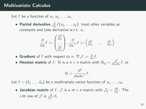
Multivariate Calculus

Let f be a function of x1, x2, . . . , xn.

• Partial derivative ∂∂xi

f (x1, . . . , xn): treat other variables as

constants and take derivative w.r.t. xi .

∂

∂xf :=

∂f∂x1

. . .∂f∂xn

,∂

∂x>f :=

(∂f∂x1

. . . ∂f∂xn

)• Gradient of f with respect to x : ∇x f := ∂

∂x f .

• Hessian matrix of f : H is a n × n matrix with Hij = ∂2

∂xi∂xjf , or

H =∂2

∂x∂x>f .

Let f = (f1, . . . , fm) be a multivariate vector function of x1, . . . , xn.

• Jacobian matrix of f : J is a m × n matrix with Jij = ∂fi∂xj

. The

i-th row of J is ∂∂x> fi .

14

Multivariate Calculus Rules

Here a and A are vector/matrix that do not depend on x = (x1, . . . , xn)ᵀ.

• ∂∂x a = 0;

• ∂∂x a

ᵀx = ∂∂x x

ᵀa = a;

• ∂∂x (xᵀa)2 = 2aaᵀx;

• ∂∂xAx = A>;

• ∂∂x x

ᵀA = A;

• ∂∂x x>Ax = (Aᵀ + A)x.

For a detailed multivariate derivatives list, see

https://www.math.uwaterloo.ca/~hwolkowi/matrixcookbook.pdf.

15

Example: Least Squares

Lets apply the equations to derive the least squares equations. Suppose

we are given matrices A ∈ Rm×n (for simplicity we assume A is full rank

so that (A>A)−1 exists) and a vector b ∈ Rm such that b 6∈ R(A). In this

situation we will not be able to find a vector x ∈ Rn such that Ax = b,

so instead we want to find a vector x such that Ax is as close as possible

to b, as measured by the square of the Euclidean norm ||Ax − b||22.

Using the fact that ||x ||22 = xᵀx , we have

||Ax − b||22 = (Ax − b)ᵀ(Ax − b) = xᵀAᵀAx − 2bᵀAx + bᵀb.

Taking the gradient with respect to x we have

∇x(xᵀAᵀAx−2bᵀAx+bᵀb) = ∇xxᵀAᵀAx−∇x2bᵀAx+∇xb

ᵀb = 2AᵀAx−2Aᵀb.

Setting this last expression equal to zero and solving for x gives the

normal equations x = (AᵀA)−1Aᵀb.

16

Probability

Sample space

• Sample space Ω is the set of all possible outcomes of a random

experiment;

• Event A is a subset of Ω, and the collection of all possible events is

denoted as F ;

• Probability measure is a function P : F → R that maps an event

into a real number which indicates the chance at which this event

happens in the experiment.

• A and B are independent events if

P(A ∩ B) = P(A)P(B).

Example: consider tossing a six-sided die,

• Ω = 1, 2, 3, 4, 5, 6;• A = 1, 2, 3, 4 ⊂ Ω is an event;

• P(A) = 46 for an even die.

17

Random Variable

• A random variable X is a function X : Ω→ R.

• Discrete random variable can only take countably many values, and

P(X = x) = P(w : X (w) = x).

• Continuous random variable can take uncountably many values, and

P(a ≤ X ≤ b) = P(w : a ≤ X (w) ≤ b).

Example: If the die gives value larger than 4, we set X = 1, and

otherwise X = 0.

• P(X = 1) = P(5, 6) = 26 ;

• P(X = 0) = P(1, 2, 3, 4) = 46 .

18

Distribution

• A cumulative distribution function (CDF) of a random variable X

(either continuous or discrete) is a function FX : R→ [0, 1] such that

FX (x) = P(X ≤ x).

• A probability mass function (PMF) of a discrete random variable

X is a function pX : R→ [0, 1] such that

pX (x) = P(X = x).

• A probability density function (PDF) of a continuous random

variable is a function fX : R→ R given by the derivative of CDF:

fX (x) =∂FX (x)

∂x.

As a result,

P(a ≤ X ≤ b) =

∫ b

a

fX (x)dx .

19

Expectation

• For a discret random variable X with PMF pX and an aribitrary

function g : R→ R, g(X ) is also a random variable whose

expectation is given by

E[g(X )] =∑x

pX (x)g(x).

• For a continuous random variable X with PDF fX , g(X ) is also a

random variable whose expectation is given by

E[g(X )] =

∫ ∞−∞

g(x)fX (x)dx .

• For two functions g1 and g2,

E[g1(X ) + g2(X )] = E[g1(X )] + E[g2(X )]

20

Variance

The variance of a random variable X is

Var[X ] = E[(X − E[X ])2

]= E[X 2]− (E[X ])2,

and the associated standard deviation is

σ(X ) =√

Var[X ].

21

Exercise: uniform distribution

Consider X ∼ uniform(0, 1) whose PDF is

fX (x) =

1, 0 ≤ x ≤ 1

0, otherwise

What’s the expectation and variance of X?

Hint:

• E[X ] =∫∞−∞ xfX (x)dx ;

• Var[X ] = E[X 2]− (E[X ])2.

22

Common distributions

• Normal distribution: X ∼ N (µ, σ2) has PDF

fX (x) =1√

2πσ2exp− 1

2σ2(x − µ)2.

• E[X ] = µ and Var[X ] = σ2.

• Bernoulli distribution: X ∼ Bernoulli(p) with 0 ≤ p ≤ 1 has PMF

PX (x) =

p, x = 1

1− p, x = 0

• E[X ] = p and Var[X ] = p(1− p).

23

Joint distributions

• For two random variables X and Y , their joint cumulative

distribution function is

FX ,Y (x , y) = P(X ≤ x ,Y ≤ y).

• For two discrete random variables X and Y , their joint probability

mass function is

pX ,Y (x , y) = P(X = x ,Y = y).

• For two continuous random variable X and Y , their joint probability

density function is

fX ,Y (x , y) =∂2FX ,Y (x , y)

∂x∂y,

so that for a set A ∈ R2 and a function g : R2 → R,

P((X ,Y ) ∈ A) =

∫∫(x,y)∈A

fX ,Y (x , y)dxdy ,

E[g(X ,Y )] =

∫∫g(x , y)fX ,Y (x , y)dxdy .

24

Independence

• Random variables X ,Y are independent if for any possible values

x , y

fX ,Y (x , y) = fX (x)fY (y), for continuous X ,Y ,

or pX ,Y (x , y) = pX (x)pY (y), for discrete X ,Y .

• For any set A = (x , y) : x ∈ A1, y ∈ A2 ⊂ R2, independent

random variables X ,Y satisfy that

P((X ,Y ) ∈ A) = P(X ∈ A1)P(Y ∈ A2).

or events w : X (w) ∈ A1 and w : Y (w) ∈ A2 are independent

events for any A1 and A2.

25

Exercise: Independence

For example, consider toss two coins consecutively, and X1 = 1 if the first

coin heads up, otherwise X1 = 0; X2 = 1 if the second coin heads up,

otherwise X2 = 0.

• Ω = (T ,T ), (H,H), (T ,H), (H,T ).• P(X1 = 1,X2 = 1) = P((H,H)) = 1

4 ;

• P(X1 = 1) = P((H,T ), (H,H)) = 12 ;

• P(X2 = 1) = P((T ,H), (H,H)) = 12 .

Thus

P(X1 = 1,X2 = 1) =1

4=

1

2× 1

2= P(X1 = 1)P(X2 = 1)..

Similarly, we can show that

P(X1 = 1,X2 = 0) = P(X1 = 1)P(X2 = 0)

P(X1 = 0,X2 = 1) = P(X1 = 0)P(X2 = 1)

P(X1 = 0,X2 = 0) = P(X1 = 0)P(X2 = 0).

26

Conditional Probability

Let A,B be two events.

• The conditional probability of A given B is defined as:

P(A|B) =P(A ∩ B)

P(B).

• If A is independent of B, we have P(A|B) = P(A), as

P(A | B) =P(A ∩ B)

P(B)=

P(A)P(B)

P(B)= P(A).

• Bayes Rule:

P(A|B) =P(B|A)P(A)

P(B).

• Chain Rule:

P(A1 ∩ A2 ∩ · · · ∩ An)

= P(A1)P(A2|A1)P(A3|A2 ∩ A1) . . .P(An|An−1 ∩ · · · ∩ A1).

27

Example: conditional probability

Consider toss a die once, and we define events

A = The value is larger than 4,B = The value is larger than 2.

Then

P(A | B) =P(A ∩ B)

P(B)

=P(5, 6 ∩ 3, 4, 5, 6)

P(3, 4, 5, 6)

=2646

=1

2.

28

Conditional Distribution

Conditional Density. The conditional probability density function of

continuous random variable X given Y = y is

fX (x |Y = y) =fX ,Y (x , y)

fY (y).

Conditional Expectation. The conditional expectation of X given

Y = y is

E(X |Y = y) =

∫ ∞−∞

xfX (x |Y = y)dx , g(y)

Conditional Variance. The conditional variance of random variable X

given Y = y is

Var[X |Y = y ] = E[(X − E(X |Y = y))2|Y = y ] , h(y).

Both E[X | Y ] and Var(X |Y ) are random variables, and their

distributions are determined by the distribution of Y .

29

Properties of Conditional Distributions

Iterated Expectation. Recall that E(X |Y ) is a function of Y , i.e., a

random variable. The law of iterative expectation states that

E[E(X |Y )] = E(X ).

Law of Total Variance. Recall that E(X |Y ) and Var(X |Y ) are both

random variables that are functions of Y . We have

Var(Y ) = E[Var(X |Y )] + Var [E(X |Y )].

30

Example: conditional distribution

Assume we throw two six-sided dice.

• What is the probability that the total of two dice will be greater

than 8 given that the first die is a 6?

• What is the expectation of the total of two dice given that the first

die is a 6?

• What is the variance of the total of two dice given that the first die

is a 6?

31

Example: conditional distribution

We use X1 to denote the value for the first die and X2 the value for the

second die.

• What is the probability that the total of two dice will be greater

than 8 given that the first die is a 6?

P(X1 + X2 > 8 | X1 = 6) =P(X1 + X2 > 8,X1 = 6)

P(X1 = 6)

=P(X1 = 6,X2 > 2)

P(X1 = 6)

=P(X1 = 6)P(X2 > 2)

P(X1 = 6)

= P(X2 > 2) =4

6.

32

Example: conditional distribution

• What is the expectation of the total of two dice given that the first

die is a 6?

Given that X1 = 6, X1 + X2 can be 7, 8, 9, 10, 11, 12, all with

probability 16 . Thus

E[X1 + X2 | X1 = 6] = 7 ∗ 1

6+ · · ·+ 12 ∗ 1

6=

57

6.

• What is the variance of the total of two dice given that the first die

is a 6? Answer: 10536 .

33

Law of large number

Consider i.i.d random variables X1, · · · ,Xn, i.e., independent random

variables with identical distributions, and an arbitrary function g .

Suppose the common expectation E[g(X1)] <∞ and common variance

Var[g(X1)] <∞,

limn→∞

1

n

n∑i=1

g(Xi ) = E[g(X1)].

Actually

• E[ 1n∑n

i=1 g(Xi )] = E[g(X1)].

• Var[ 1n∑n

i=1 g(Xi )] = 1n Var[g(X )].

34

Resources

Resources

• Linear algebra:

http://cs229.stanford.edu/summer2019/cs229-linalg.pdf

• Matrix calculus: https:

//www.math.uwaterloo.ca/~hwolkowi/matrixcookbook.pdf

• Probability:

http://cs229.stanford.edu/summer2019/cs229-prob.pdf and

All of Statistics by Larry Wasserman.

35