Math Camp

September 16, 2017Unit 2

MSSM ProgramColumbia UniversityDr. Satyajit Bose

Math Camp

Interlude

Partial Derivatives

• Recall:The derivative f'(x) of a function f(x) is the slope of f(x).

• Alternatively, the derivative f'(x) is the rate at which the function f(x) is changing with respect to changes in the variable x.

• What is the analogue of the derivative in a multivariate function?

Partial Derivatives

• The partial derivative of f(x,y) with respect to x, written ∂f/ ∂x, is the derivative of f(x,y) where y is treated as a constant and f(x,y) is considered as if it were a function of x alone.

• The partial derivative of f(x,y) with respect to y, written ∂f/ ∂y, is the derivative of f(x,y) where x is treated as a constant and f(x,y) is considered as if it were a function of y alone.

Interpretation of Partial Derivatives

• Since ∂f/ ∂x is simply the ordinary derivative with y held constant, ∂f/ ∂x gives the rate of change of f(x,y) with respect to x for y held constant.

• Alternatively, keeping y constant and increasing x by one (small) unit produces a change in f(x,y) that is approximately given by ∂f/ ∂x .

Partial Differentiation

• f(x,y) = 5x3y2

• Compute ∂f/ ∂x– Think of f(x,y) as [5y2]x3 where

the brackets facilitate treating y as a constant

– Differentiate with respect to x• ∂f/ ∂x = 3[5y2]x2 = 15x2y2

Partial Differentiation

• f(x,y) = (4x + 3y - 5)8

• Compute ∂f/ ∂x– Think of f(x,y) as (4x + [3y - 5])8

where the brackets facilitate treating y as a constant

– Differentiate with respect to x• ∂f/ ∂x = 8(4x + [3y – 5])7 * 4 = 32(4x + [3y – 5])7

Example: Heat Loss• Recall the heat loss function as function of

building dimensions.– f(x,y,z) = 11xy + 14yz +15xz

• Calculate and interpret ∂f/ ∂x if (x,y,z) = (10,7,5)

• ∂f/ ∂x = 11y + 15z• ∂f/ ∂x at (10,7,5) = 11*7 + 15*5 = 152• The quantity ∂f/ ∂x is the marginal heat loss

with respect to a change in x. With current dimensions (10,7,5), if x were to increase by 1 unit, then the approximate additional heat loss would be 152 units.

Multivariate Optimization

• As with univariate optimization, critical points of a multivariate function are characterized by zero (partial) slopes.

First Order Condition

• For a function of 2 variables f(x,y) that has either a relative maximum or minimum at (x*,y*),

∂f(x*,y*)/∂x = 0AND∂f(x*,y*)/∂y = 0

Example: Energy Efficiency• Recall the heat loss function as function of

building dimensions.– f(x,y,z) = 11xy + 14yz +15xz

• Suppose we want to design a rectangular building with volume 147,840 cubic feet which has minimal heat loss.

• We must minimize the function f(x,y,z) s.t. xyz = 147,840

Example: Energy Efficiency• We must minimize the function f(x,y,z) s.t.

xyz = 147,840• For simplicity, denote 147,840 = Vxyz = V• Express z in terms of x,y and Vz = V/xy• Substitute into f(x,y,z)f(x,y,z(x,y,V)) = 11xy + 14y(V/xy) + 15x(V/xy)

= 11xy + 14V/x + 15V/y

Example: Energy Efficiency• To minimize this function, we compute

partial derivatives w.r.t. x and y; then we equate them to zero to meet the first order condition (ignoring the second order condition for now)

f(x,y,z(x,y,V)) = 11xy + 14V/x + 15V/y• ∂f/∂x = 11y – 14V/x2

• ∂f/∂y = 11x – 15V/y2

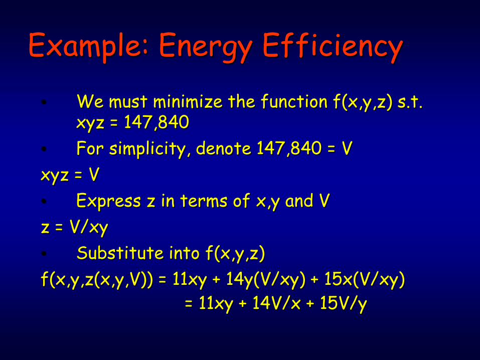
Example: Energy Efficiency• Now equate the partial derivatives to zero∂f/∂x = 11y – 14V/x2 = 0∂f/∂y = 11x – 15V/y2 = 0• These equations give:y = 14V/(11x2)11xy2 = 15V• Substitute for y in the second equation:11x(14V/11x2)2 = 15V142V2/11x3 = 15Vx3 = 142V/11*15

Example: Energy Efficiency• x3 = 142V/11*15• Using V = 147,840 ⇒ x3 = 175,616 or x = 56• Using y = 14V/11x2 ⇒ y = 14*147,840/11*562

= 60• Using z = V/xy ⇒ z = 147,840/56*60 = 44• The building which minimizes heat loss

should be 56ft long, 60ft wide and 44ft high.

Saddle Point

Second Order Condition

• For a function of 2 variables f(x,y) s.t. at (x*,y*),

∂f(x*,y*)/∂x = 0 and ∂f(x*,y*)/∂y = 0Define D(x,y) = (∂2f/∂x2)(∂2f/∂y2) - (∂2f/∂x∂y)2

Second Order Condition

• If D(x,y) > 0 and (∂2f(x*,y*)/∂x2) > 0Then f(x,y) has a relative minimum at (x*,y*)• If D(x,y) > 0 and (∂2f(x*,y*)/∂x2) < 0

Then f(x,y) has a relative maximum at (x*,y*)

• If D(x,y) < 0Then f(x,y) has neither a relative maximum

nor a relative minimum at (x*,y*)• If D(x,y) = 0, then no conclusion can be

drawn from this test.

Math Camp

Interlude

Fundamental Calculus Problems

1. Find the slope of a curve at a point.⇒ Find the derivative.

2. Find the area of a region under a curve.⇒ Approximate the area using a collection

of regular shapes whose areas can be computed geometrically.

⇒ Or find the antiderivative or the integral.

Derivatives

• Recall:The derivative f'(x) of a function f(x) is the slope of f(x).

• Alternatively, the derivative f'(x) is the rate at which the function f(x) is changing with respect to changes in the variable x.

• In many applications, we need to proceed in reverse: we know the rate of change of the function i.e. we know f’(x) but must deduce f(x).

The Antiderivative

• Suppose that f(x) is a given function and F(x) is a function having f(x) as its derivative, i.e. F’(x) = f(x). We call F(x) an integral or an antiderivative of f(x).

ExampleFind the antiderivative of f(x) = x2.

Reverse the general power rule to yield:F(x) could be 1/3x3

or 1/3x3 + 1 or 1/3x3 + 5or 1/3x3 + c, where c is any constant

ExampleFind the antiderivative of f(x) = 2x –

(1/x2)

Reverse the sum rule and the general power rule to yield:

F(x) is x2 + 1/x + c, where c is any constant

The Indefinite IntegralSuppose that f(x) is a function whose

antiderivatives are F(x) + c. This is denoted:∫f(x) dx = F(x) + c

The symbol ∫ is the integral sign. The notation ∫ f(x) dx is the indefinite integral. “dx” denotes that the anti-differentiation is with respect to the variable x.

Example

Determine ∫ xr dx where r is a constant not equal to –1

Note xr = ((r+1)/(r+1)) xr

Using the power rule in reverse,∫ xr dx = (xr+1)/(r+1) + c

r ≠ -1 since division by 0 is not defined.What if r = -1?

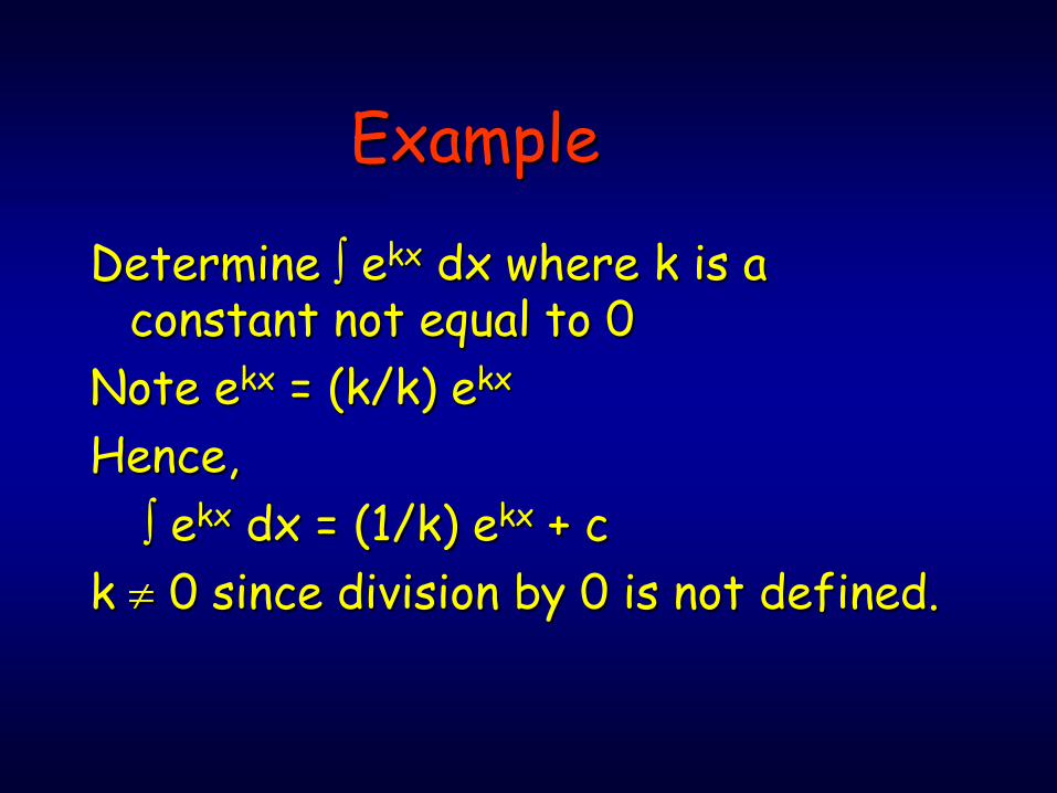
Example

Determine ∫ ekx dx where k is a constant not equal to 0

Note ekx = (k/k) ekx

Hence,∫ ekx dx = (1/k) ekx + c

k ≠ 0 since division by 0 is not defined.

Integration Rules

1. Sum Rule∫ [f(x) + g(x)] dx = ∫ f(x) dx + ∫ g(x)

dx2. Constant Multiple Rule

∫ kf(x) dx = k ∫ f(x) dx where k is a constant

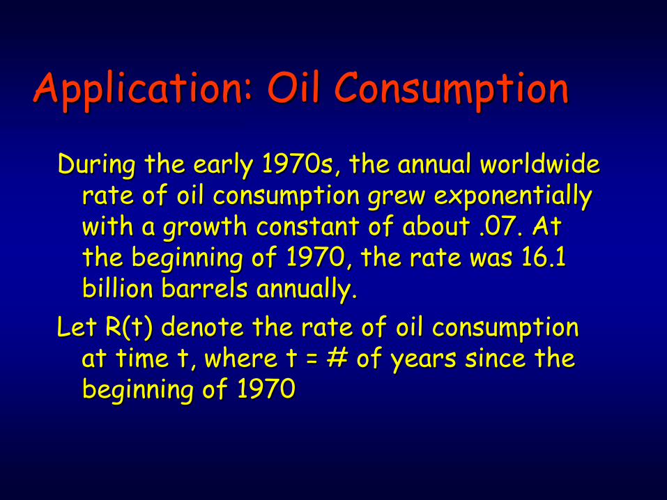
Application: Oil ConsumptionDuring the early 1970s, the annual worldwide

rate of oil consumption grew exponentially with a growth constant of about .07. At the beginning of 1970, the rate was 16.1 billion barrels annually.

Let R(t) denote the rate of oil consumption at time t, where t = # of years since the beginning of 1970

Application: Oil ConsumptionUse the function R(t) = 16.1e0.07t to

determine the total amount of oil that would have been consumed from 1970 to 1980 had this rate of consumption continued throughout the decade.

Let T(t) = total oil consumed from 1970 to time t

T ’(t) is the rate of oil consumption (by definition of the derivative)

Hence T ’(t) = R(t)Hence, T(t) is an antiderivative of R(t)

Application: Oil ConsumptionT(t) = ∫ 16.1e0.07t dt = 16.1 ∫ e0.07t dt = 16.1 ( (1/0.07) e0.07t ) + c= 230e0.07t + cWe know that T(0) = 0Hence, 230e0.07×0 + c = 0 ⇒ c = -230Hence, T(t) = 230e0.07t - 230

Application: Oil Consumption

The total amount of oil that would have been consumed from 1970 to 1980 is

T(10) = 230e0.7 - 230 ≈ 233 billion barrels

Application: Marginal CostA factory’s marginal cost function is(1/100)x2 – 2x + 120, where x is qty produced

per day. The factory has fixed costs of $1000 per day. Find the cost function.

C’(x) = (1/100)x2 – 2x + 120C(x) = ∫ [(1/100)x2 – 2x + 120] dx= (1/300)x3 – x2 + 120x + c

Application: Marginal Cost

C(0) = 1000⇒1000 = (1/300)03 – 02 + 120(0) + c⇒c = 1000C(x) = (1/300)x3 – x2 + 120x + 1000

Math Camp

Interlude

Interpretation of the Integral

How do we compute the shaded area under the curve?

Riemann Sum ApproximationPartition the interval [a,b] into n equal sub-

intervals, each of width ∆x.For each sub-interval, choose a

representative value of x denoted x1, x2, …, xn.

The shaded area can be approximated by summing the areas of the n rectangles which approximately cover the area under the curve:

[Area of rectangular approximation] =f(x1)∆x + f(x2)∆x + … + f(xn)∆x

Definite IntegralsThe definite integral of f(x) from a to b is

denoted by

The definite integral is the limit of the Riemann sum as ∆x → 0.

If f(x) is continuous and nonnegative in [a,b] then the definite integral = area under the graph

∫b

af(x)dx

Fundamental Theorem of Calculus

Suppose that f(x) is continuous on the interval [a,b] and let F(x) be an antiderivative of f(x). Then

)()()( aFbFdxxfb

a−=∫

ExampleUse the fundamental theorem of calculus to

evaluate the following definite integrals:a)

b)

( )dxx∫2

1

dxx∫ −5

0)42(

Application: Oil Consumption

During the early 1970s, the annual worldwide rate of oil consumption was R(t) = 16.1e0.07t where t = # of years since the beginning of 1970

Determine the amount of oil consumed from 1972 to 1974.

Represent this amount as an area.

Application: Oil ConsumptionT(4) – T(2) = oil consumed from 1972 to

1974T’(t) = R(t)

≈ 39.76 billion barrels

∫∫ ==−4

2

07.04

21.16)()2()4( dtedttRTT t

)2(07.0)4(07.04

2

07.0 23023007.01.16 eee t −==

Application: Oil ConsumptionT(4) – T(2) can be represented as the

area under the curve of y = R(t) in the interval [2,4]

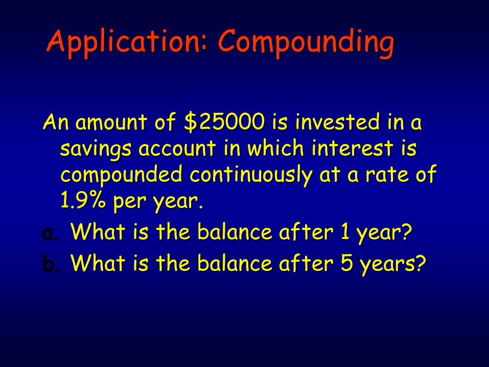
Application: Compounding

An amount of $25000 is invested in a savings account in which interest is compounded continuously at a rate of 1.9% per year.

a. What is the balance after 1 year? b. What is the balance after 5 years?

For continuously compounding interest, we can use the formula A=Pert, where A is the future value and P is the present value. In this case, we are solving for A.

What we know:P=25000 the initial investmentr=0.019 the interest ratet=1 time (in years)This gives us A = 25000e^{(0.019)(1)} = $25480

Application: Compounding

Application: CompoundingAt an interest rate of 5.8% compounded

continuously, when will an investment of $15000 double itself?

In this example we want to know a time. Again we use the formula A=Pe^{rt}, so we are solving for t. What we know:

r=0.058P=15000Since the final amount must be double the principal,

we have A=30000. Substituting into the formula gives us 30000=15000e^{(0.058)t}

Application: CompoundingAnd solving for t yields:

( )

951.11058.0

2ln058.02ln

ln2ln2

1500015000

1500030000

058.0

058.0

058.0

=

=

==

=

=

t

t

te

e

e

t

t

t

Math Camp

Interlude

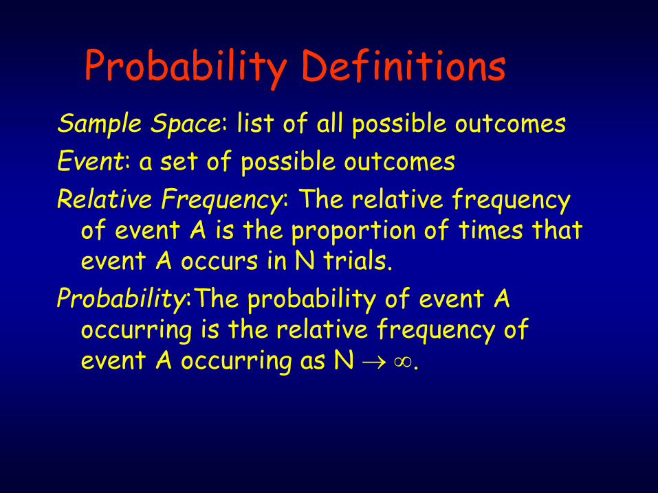
Probability DefinitionsSample Space: list of all possible outcomesEvent: a set of possible outcomesRelative Frequency: The relative frequency

of event A is the proportion of times that event A occurs in N trials.

Probability:The probability of event A occurring is the relative frequency of event A occurring as N → ∞.

Properties of EventsMutually Exclusive: Events A and B are

mutually exclusive if and only ifP(A or B) ≡ P(A ∪ B) = P(A) + P(B)

Collectively Exhaustive: The events A or B or C are collectively exhaustive ifP(A or B or C) ≡ P(A ∪ B ∪ C) = 1

Partition: A collection of events which are mutually exclusive and collectively exhaustive is known as a partition of the sample space.

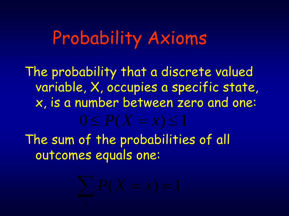
Probability Axioms

The probability that a discrete valued variable, X, occupies a specific state, x, is a number between zero and one:

The sum of the probabilities of all outcomes equals one:

1)( ==∑x

xXP

1)(0 ≤=≤ xXP

Venn Diagrams

Union A∪B Intersection A∩B

P(A ∪ B) = P(A) + P(B) - P(A ∩ B)

Note: If A, B are mutually exclusive P(A ∩ B) = 0

Venn Diagrams

Exclusive Or

A ⊕ B ≡ (A∪B) ∩ (A∩B)’

Venn Diagrams

Math Camp

Interlude

Conditional ProbabilityOften, we want to know the probability of an

event given the occurrence of some other event. For example, the probability of an oil tanker spill, given that the captain of the tanker is drunk.

Is the probability of an oil spill given a drunk captain higher or lower than the unconditional probability of an oil spill?

Conditional Probability

The probability of event B occurring conditional on event A equals the probability of events A and B occurring divided by the probability of A occurring:

P(B|A) = P(A ∩ B) / P(A)

Example

Suppose a die is rolled. Event A is the roll takes a value less than 4. Event B is that the roll is an odd number. What is the probability of the roll being an odd number given that event A has occurred?

Event A = 1, 2, or 3 is rolled.Event B = 1, 3, or 5 is rolled.Of the 3 values that comprise event A, 2 are associated with

event B. So the probability of event B occurring given event A is 2/3.

Now use the formula. Events A and B occur when a 1 is thrown or when a 3 is thrown. The probability of one of these happening is 1/6 + 1/6 = 1/3.

P(A ∩ B) = 1/3 P(A) = ½ ⇒ P(B|A) = 1/3 ÷ ½ = 2/3

Independent Events

In a casual sense, two events are independent if knowledge that one event has occurred is no cause to adjust the probability of the other event occurring.

Two events, A and B, are independent, if P(A|B) = P(A)

Independent Events

If two events, A and B, are independent, then

P(A ∩ B) = P(A) P(B)Show that this follows from the

definitions of conditional probability and independence.

Birthday Problem

In a set of n randomly chosen people, there is a surprisingly high probability that some pair of them will have the same birthday.

E.G. In a set of 23 randomly chosen people, the probability that some pair of them will have the same birthday is approximately 51%.

Birthday ProblemIn a group of 23, there 253 possible pairs to check for the same birthday:

Person 1 could have the same birthday as 22 others, Person 2 could have the same birthday as 21 others, etc.

22+21+20+19+…+2+1 = 253P(A) = probability of a matchP(A’) = probability of no matchP(A) = 1 – P(A’)Number each person 1 to 23. Analyze each person in turn. Define events 1 to

23 as the corresponding person not sharing his/her birthday with any of the previously analyzed people .

Birthday ProblemP(1) = 365/365P(2) = 364/365P(3) = 363/365 etc.P(23) = 343/365

Due to independence, we can multiply probabilities of these eventsP(A’) = P(1)×P(2) ×P(3)… ×P(23) = (1/365)23 × (365 ×364 ×363 ×… ×343)

P(A’) = 0.493P(A) = 0.507

Bayes Theorem

Consider two events A and B. These two events give rise to two other events: not A and not B.

These are denoted A’ and B’ or ¬A and ¬B.

Note that A and A’ comprise a partition of the sample space.

Bayes TheoremHow does the probability of B change if we

know whether or not A has occurred? In other words, what is the conditional probability P(B|A)?

P(B |A) = P(A ∩ B) / P(A) by definition.Bayes Theorem expresses the conditional

probability P(B|A) using probabilities which may be easier to compute than P(A ∩ B) or P(A).

Bayes Theorem

Or

)()()()()()(

)(BAPBPBAPBP

BAPBPABP

¬⋅¬+⋅⋅

=

)()()(

)(AP

BAPBPABP

⋅=

ExampleAll people in a population are tested for a medical

condition (e.g. measles antibody). Suppose you have the following information about this medical condition and a laboratory test for this condition:

• The chance of a random draw from the population having the medical condition is 0.001

• The chance of a false positive test result from the lab test is 0.01

• The chance of a false negative test result for the lab test is 0.002

ExampleWithout the test, it is rational to believe that your

chance of having the condition is 0.001. If the test comes back positive, what are the chances you have the medical condition?

Event Definition:A : You have the medical condition.¬ A :You do not have the medical condition.B : You have a positive test result.¬ B : You have a negative test result.

ExampleP(A) = 0.001False positives: P(B| ¬ A ) = 0.01False negatives: P(¬ B| A ) = 0.002Also, compute complements:P(¬ A) = 0.999P(¬ B| ¬ A ) = 0.99P(B| A ) = 0.998

Example

0908.01.999.998.001.

998.001.)()()()(

)()()(

=×+×

×=

¬⋅¬+⋅⋅

=ABPAPABPAP

ABPAPBAP

Hence, having tested positive, there is 9.08% chance that you have the medical condition.

Math Camp

Interlude

Probability DistributionsRandom Variable: is a function that assigns a

number to each possible outcome in a chance experiment.

Example: Roll of 2 dice

Sum of dice

2 3 … 7 … 11 12

P 1/36 2/36 … 6/36 … 2/36 1/36

Discrete Probability Distribution

The probability distribution function P(x) is the function that assigns a number to each possible outcome s.t.

Where xi is the ith value that the random variable can take on, P(⋅) is the probability the random variable takes on a particular value, and n is the number of possible random values.

∑=

=n

iixP

11)(

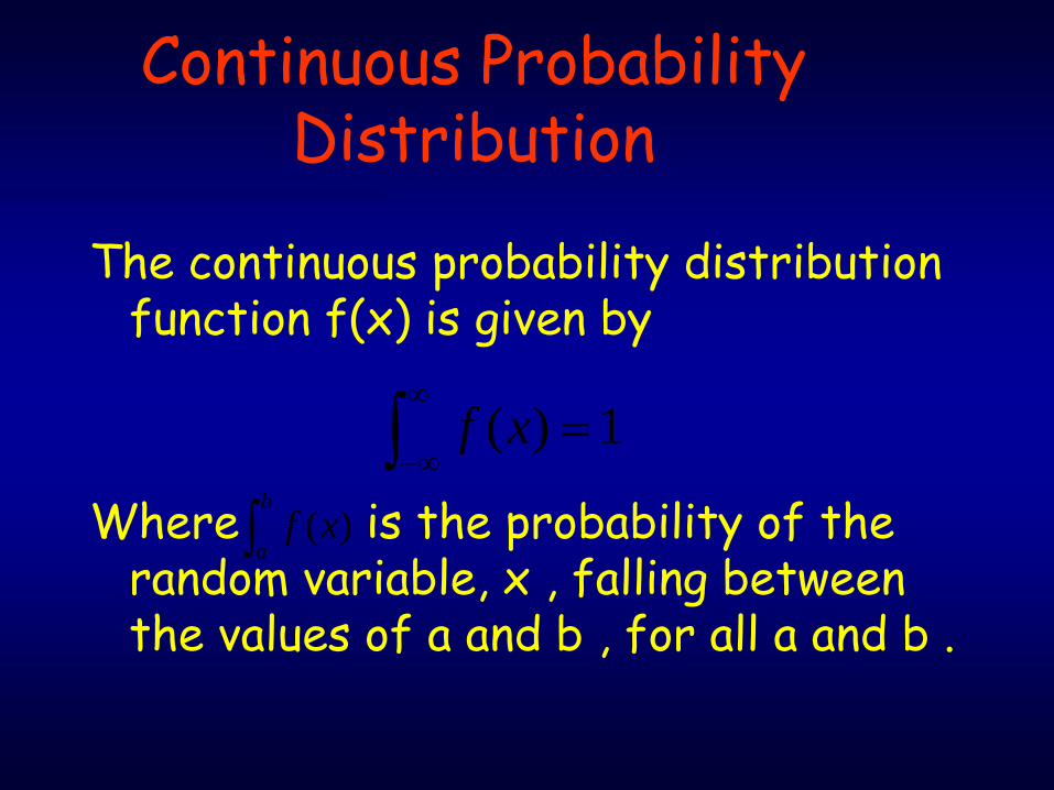
Continuous Probability Distribution

The continuous probability distribution function f(x) is given by

Where is the probability of the random variable, x , falling between the values of a and b , for all a and b .

1)( =∫∞

∞−xf

∫b

axf )(

Cumulative Distribution (Density)Functions

Related to probability distribution functions are cumulative distribution or density functions (CDFs). The density function relate the value of a random variable with the probability of the random variable being less than or equal to that value.

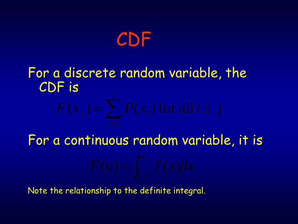
CDFFor a discrete random variable, the

CDF is

For a continuous random variable, it is

Note the relationship to the definite integral.

∑=

≤=j

iij jixPxF

1 allfor )()(

dxxfaF ∫∞

∞−= )()(

Math Camp

Interlude

StatisticsStatistics is concerned with collection,

organization and interpretation of numerical data:

• Aims to infer general knowledge from samples

• Explores data to find tentative patterns (hypotheses)

• Tests the validity of hypotheses

MeasurementObjects to be measured in statistics

are often coded as :• Nominal variables (qualitiative or

categorical)• Ordinal variables (ranked)• Scale variables (continuous)

Central Tendency

A symmetric distribution

An asymmetric distribution

Dispersion