Embed Size (px)
Citation preview

Math 7510: Sheaves on Manifolds
Taught by Allen Knutson
Notes by David [email protected]
Cornell UniversityFall 2016
Last updated November 30, 2016.The latest version is online here.

Contents
1 Noncommutative Algebra . . . . . . . . . . . . . . . . . . . . . . . . . 41.1 Stuff that has nothing to do with D-modules . . . . . . . . . . . 81.2 Application: Projective duality . . . . . . . . . . . . . . . . . . . 91.3 Rees Algebra . . . . . . . . . . . . . . . . . . . . . . . . . . . . . . . 111.4 Back to representation theory . . . . . . . . . . . . . . . . . . . . 13
2 CSM Classes . . . . . . . . . . . . . . . . . . . . . . . . . . . . . . . . . 142.1 The Deligne-Grothendieck Conjecture . . . . . . . . . . . . . . . 172.2 Toric Varieties . . . . . . . . . . . . . . . . . . . . . . . . . . . . . 192.3 CSM Classes on Toric Varieties . . . . . . . . . . . . . . . . . . . 202.4 Independence for Deligne-Grothendieck . . . . . . . . . . . . . . 232.5 Bott-Samelson Manifolds . . . . . . . . . . . . . . . . . . . . . . . 25
3 Derived Categories . . . . . . . . . . . . . . . . . . . . . . . . . . . . . 273.1 General remarks on Localizations . . . . . . . . . . . . . . . . . . 273.2 Triangulated Categories . . . . . . . . . . . . . . . . . . . . . . . 283.3 Homotopy Categories . . . . . . . . . . . . . . . . . . . . . . . . 293.4 Verdier Quotients and Derived Categories . . . . . . . . . . . . . 303.5 Derived Functors and DbpCohpXqq . . . . . . . . . . . . . . . . . . 313.6 Derived Categories of Sheaves . . . . . . . . . . . . . . . . . . . 323.7 Bondal-Orlov Theorem . . . . . . . . . . . . . . . . . . . . . . . . 333.8 Fourier-Mukai Transform . . . . . . . . . . . . . . . . . . . . . . 333.9 Exceptional Collections . . . . . . . . . . . . . . . . . . . . . . . . 34
4 Back to CSM Classes . . . . . . . . . . . . . . . . . . . . . . . . . . . . 364.1 Demazure Products . . . . . . . . . . . . . . . . . . . . . . . . . . 364.2 Variations on Bott-Samelsons . . . . . . . . . . . . . . . . . . . . 374.3 Abstract Toric Varieties . . . . . . . . . . . . . . . . . . . . . . . . 434.4 Bott-Samelsons as Homology Classes . . . . . . . . . . . . . . . 444.5 The Anderson-Jantzen-Soergel/Billey Formula . . . . . . . . . . 464.6 Deodhar decomposition of BSQ . . . . . . . . . . . . . . . . . . . 474.7 CSM classes of Bott-Samelsons . . . . . . . . . . . . . . . . . . . 484.8 A few variations on Bott-Samelsons . . . . . . . . . . . . . . . . . 51
5 Perverse Sheaves . . . . . . . . . . . . . . . . . . . . . . . . . . . . . . 525.1 f! and f ! . . . . . . . . . . . . . . . . . . . . . . . . . . . . . . . . 52
6 Other stuff . . . . . . . . . . . . . . . . . . . . . . . . . . . . . . . . . . 536.1 Brick Manifolds . . . . . . . . . . . . . . . . . . . . . . . . . . . . 546.2 Gross-Hacking-Keel . . . . . . . . . . . . . . . . . . . . . . . . . . 556.3 An application of Brick manifolds . . . . . . . . . . . . . . . . . 56
1

6.4 Duistermaat-Heckman Theorem . . . . . . . . . . . . . . . . . . 576.5 The Cartan model of H˚TpMq . . . . . . . . . . . . . . . . . . . . . 596.6 Duistermaat-Heckman Measures . . . . . . . . . . . . . . . . . . 606.7 Spherical actions . . . . . . . . . . . . . . . . . . . . . . . . . . . 646.8 D-modules of twisted differential operators . . . . . . . . . . . . 666.9 A bit of silliness . . . . . . . . . . . . . . . . . . . . . . . . . . . . 696.10 Calabi-Yau, Hirzebruch-Riemann-Roch . . . . . . . . . . . . . . 70
2

Contents by Lecture
Lecture 01 on August 29, 2016 . . . . . . . . . . . . . . . . . . . . . . . . . 4
Lecture 02 on August 31, 2016 . . . . . . . . . . . . . . . . . . . . . . . . . 7
Lecture 03 on September 7, 2016 . . . . . . . . . . . . . . . . . . . . . . . . 10
Lecture 04 on September 12, 2016 . . . . . . . . . . . . . . . . . . . . . . . 13
Lecture 05 on September 14, 2016 . . . . . . . . . . . . . . . . . . . . . . . 17
Lecture 06 on September 19, 2016 . . . . . . . . . . . . . . . . . . . . . . . 20
Lecture 07 on September 21, 2016 . . . . . . . . . . . . . . . . . . . . . . . 23
Lecture 08 on September 26, 2016 . . . . . . . . . . . . . . . . . . . . . . . 26
Lecture 09 on September 28, 2016 . . . . . . . . . . . . . . . . . . . . . . . 32
Lecture 10 on October 12, 2016 . . . . . . . . . . . . . . . . . . . . . . . . . 36
Lecture 11 on October 17, 2016 . . . . . . . . . . . . . . . . . . . . . . . . . 39
Lecture 12 on October 19, 2016 . . . . . . . . . . . . . . . . . . . . . . . . . 42
Lecture 13 on October 24, 2016 . . . . . . . . . . . . . . . . . . . . . . . . . 46
Lecture 14 on October 26, 2016 . . . . . . . . . . . . . . . . . . . . . . . . . 48
Lecture 15 on October 31, 2016 . . . . . . . . . . . . . . . . . . . . . . . . . . 51
Lecture 16 on November 03, 2016 . . . . . . . . . . . . . . . . . . . . . . . 54
Lecture 17 on November 07, 2016 . . . . . . . . . . . . . . . . . . . . . . . 56
Lecture 18 on November 14, 2016 . . . . . . . . . . . . . . . . . . . . . . . 60
Lecture 19 on November 16, 2016 . . . . . . . . . . . . . . . . . . . . . . . 62
Lecture 20 on November 21, 2016 . . . . . . . . . . . . . . . . . . . . . . . 64
Lecture 21 on November 28, 2016 . . . . . . . . . . . . . . . . . . . . . . . 66
Lecture 22 on November 30, 2016 . . . . . . . . . . . . . . . . . . . . . . . 69
3

Lecture 01: Noncommutative Algebra August 29, 2016
Administrative
There is now a webpage with a list of things we want to understand by theend of the course, including papers that we’ll hopefully have the backgroundto read by the end of the course. Primarily we want to follow Kashiwara andShapira’s book Sheaves on Manifolds.
1 Noncommutative Algebra
Even though the course is geometry through and through, the initial motivationcomes from noncommuative algebra.
Definition 1.1. If g is a Lie algebra, we get a noncommutative associative algebraUpgq called the universal enveloping algebra that is defined as
Uhpgq “TpgqL
xXY´YX´ hrX, Ysy ,
whereTg “
à
nPN
gbn.
Theorem 1.2 (Poincare-Birkhoff-Witt). This is flat in h if and only if these gener-ators are a Grobner basis if and only if
gr Upgq :“à
nPN
ˆ
UpgqdegďnL
Upgqdegďn´1
˙
– Sym g
Remark 1.3.
Upgq ZpUpgqq pUpgqqg-invariants –
Sym g pSym gqG
gr
Ě
Ě
pUgqg-invariants – pSym gqg if the action of g on Ug is completely reducible.pSym gqg – pSym gqG if g “ LiepGq is connected.pSym gqG – pSym lqW where W is the Weyl group.
The linear term in h of the product on Uhgh2 gives a Poisson (Lie) brackett´,´u on Sym g. A Poisson bracket is a Lie bracket such that
r f , ghs “ t f , guh` gt f , hu.
This one in particular satisfies
tX, Yu “ rX, Ys
4

Lecture 01: Noncommutative Algebra August 29, 2016
Definition 1.4. M is a Poisson manifold if the set of functions FunpMq on M isequipped with a Poisson bracket.
This gives us (a unique) π P ΓpM;Ź2 TMq, called an alternating 2-tensor.
The Poisson bracket is related to π by
t f , gu “ xπ, d f ^ dgy
We can’t define the Poisson bracket this way from any arbitrary alternating2-tensor, because we aren’t guaranteed that the resulting bracket will satisfy theJacobi identity. There needs to be an alternate definition.
π gives a map π¨ : T˚M Ñ TM given by α ÞÑ xπ, α^´y.
xα, πy “ÿ
αp~viq b ~wi.
Example 1.5. If G “ SOp3, Rq acts on sop3q˚ “ R3 with the usual action ofsop3q.
???
Definition 1.6. M is (Poisson) symplectic if π¨ : T˚M Ñ TM is onto for allm P M
Example 1.7. M “ R2, π “ f px, yqddx^ddy for some nowhere vanishing f px, yq
(iff f is symplectic), π Poisson.In this case, the inverse ω : TM Ñ T˚M exists, or ω P
Ź2 T˚M is thesymplectic form.
Remember that we needed extra conditions so that an alternating 2-tensor π
defines a Poisson bracket t f , gu “ xπ, d f ^ dgy that satisfies the Jacobi identity?Well, that condition turns out to be that ω is closed, that is, dω “ 0.
Theorem 1.8. If π¨ has constant rank near m P M, then M near m has a foliationby submanifolds whose tangent spaces are the images of π¨, and are naturallysymplectic.
Example 1.9 (Bad example). Let R act on R4 by
x ÞÑ
»
—
—
–
cos x sin x´ sin x cos x
?2 cos x
?2 sin x
´?
2 sin x?
2 cos x
fi
ffi
ffi
fl
Then take G “ R˙R4. The orbits on g˚ are only locally closed. This is theirrational orbits on the torus issue.
Definition 1.10. Let M be a smooth manifold. Let VecpMq be the sheaf of vectorfields on M. This is a Lie algebra.
5

Lecture 01: Noncommutative Algebra August 29, 2016
Definition 1.11. DM :“ UpVecpMqq, the universal enveloping algebra of VecpMq.Recall that the universal enveloping algebra is a quotient of the tensor algebra.But we’re not tensoring over C, rather over OM, the set of functions on M.
There is an action of VecM on OM, because derivatives act on functions.Therefore, DM acts on OM as differential operators (higher order derivatives).
Being a universal enveloping algebra, DpMq has a degeneration, via theassociated graded algebra, to SympVecMq.
So what is SympVecMq? This is
SympΓpM; TMqq “ ΓpM; Sym TMq “ p˚pOT˚Mq
Where p : T˚M Ñ M, and this is the pushforward of the sheaf on T˚M to thesheaf on M.
Then T˚M is Poisson, and even better, symplectic, and the symplectic 2-formis given as follows.
If pm, f q P T˚M for m P M and f P T˚m M, let ~v, ~w P Tpm, f qpT˚Mq. We have
ωp~v, ~wq “ exercise. There’s only one possibility up to sign.
Starting Point
Remark 1.12. Now let’s put some of this stuff together. Let’s say we’re in-terested in representation theory. If we have G acting on some vector spaceV irreducibly, then we get an action of g and Upgq on this vector space aswell. Thus ZpUpgqq acts on V by scalars, by Schur’s lemma. This gives a mapZpUpgqq Ñ R defining this action.
Going backwards, we get a point in SpecpZpUpgqqq.
G-orbit closure g˚
pt Spec ZpUpgqq – g˚G
Example 1.13. G acts on C, and the G-orbit closure is the fiber over 0 in thecharacteristic polynomial map. This is the so-called nilpotent cone N.
If instead G “ GLnpCq, then N is the nilpotent matrices.
Definition 1.14. A DM-module is a sheaf over M with an action of VecpMq, orequivalently an action of DM.
Example 1.15. We already saw that DM acts on OM.
Example 1.16. Let M “ C “ SpecpCrzsq. Then the global sections of DM is thealgebra
C
„
ddz
, pzNB„
ddz
, pz
´ 1F
6

Lecture 02: Noncommutative Algebra August 31, 2016
The hat means that this isn’t z, but rather multiplication by z, because it’s anoperator not a variable. DM acts on Crzs by taking derivatives or multiplyingby z.
Here are three DM-modules for this M. They are all cyclic.
D-module generator linear ODE (relation)Functions on C 1 ddz
Distributions supported at 0 δ0 (delta function) pzFunctions on Cˆ z´1 ddzpz
We find the appropriate D-module by quotienting by the right ideal generatedby the linear ODE.
(Remark: The last is not finitely generated over OM, but it is over DM. )What are the associated graded modules? Write grDM “ Crξ, zsxrξ, zs “ 0y.
D-module pgrDM)-module Spec Ď T˚C – C2
Functions on C ξ “ 0 z-axisDistributions supported at 0 z “ 0 ξ-axis
Functions on Cˆ ξz “ 0 both axes
We think of the picture as having a horizontal z-axis and a vertical ξ-axis.
Let’s be concrete and actually prove some things this time. Let A be anoncommutative graded algebra, A “
Ť
iPN Ai, with Ai ď Ai`1, Ai Aj Ď Ai`j.Then
gr A :“à AiAi´1 .
This is the associated graded algebra. We impose an extra assumption here,namely that gr A is commutative.
Now suppose that a, b P gr A homogeneous with a P AiAi´1, b P AjAj´1,with lifts a P Ai, b P Aj.
Then define the poisson bracket of a and b by
ta, bu “ pab´ baq ` Ai`j´2 PAi`j´1Ai`j´2
The commutator ab´ ba is an element of Ai`j´1 because gr A is commutative,so the terms in Ai`j cancel.
Definition 1.17. Given a DM-module F , a good (increasing) filtration Fi is
(1) compatible with pDMqj. Therefore, OT˚M “ grDM
œ
grF .
7

Lecture 02: Stuff that has nothing to do with D-modules August 31, 2016
(2) For all grF coherent over T˚M.
For D-modules, you should picture distributions on a submanifold valuedin a vector bundle with connection.
Remark 1.18 (Theorems to Come).
(1) supppgrFq Ď T˚M is coisotropic (at its smooth points). There are twoways to explain what coisotropic means. First, if C is smooth and con-tained in S symplectic, then pTcCqK ď TcC. The second version is thatif I “ annpgrFq, then tI, Iu Ď I, that is, I is closed under the Poissonbracket.
(2) The characteristic cycle (often denoted ss for singular support), definedby
ÿ
top-dim components C of support
multCrCs
is independent of the choice of filtration. (This lives inside formal Z-linearcombinations of subvarieties of fixed dimension).
Definition 1.19. Let S be a symplectic manifold. L Ď S is Lagrangian if it iscoisotropic and dim L “ 1
2 dim S.
Definition 1.20. A D-module F is holonomic if the singular support sspFq isLagrangian, and not just coisotropic.
Definition 1.21. If L Ď T˚M is Lagrangian, then it is conical if invariant underscaling the fibers of T˚M.
Example 1.22. The singular support of a D-module is necessarily conical.In T˚R, only get the z-axis or translates of the ξ-axis (where the axes are as
before in the three examples of D-modules).
1.1 Stuff that has nothing to do with D-modules
Definition 1.23. If Y Ď M is smooth and locally closed (for example a curvewithout endpoints), the conormal bundle is
CY :“ tpm,~vq P T˚M | m P Y,~v K TmYu.
Example 1.24.
(1) The conormal bundle of M is just the zero section.
(2) The conormal bundle to a point y is T˚y M.
8

Lecture 02: Application: Projective duality August 31, 2016
Remark 1.25 (Fun Fact). The conormal bundle is automatically conical andLagrangian.
The locally closed condition on Y is irritating to work with, especially inalgebraic geometry.
Definition 1.26. If Y is closed and irreducible and M smooth, with Y Ď M, thenthe conormal variety is
CY “ CYreg.
This is conical, Lagrangian, and irreducible.
Example 1.27. Let M be a vector space and Y a subspace. Then T˚M – MˆM˚
and CY “ YˆYK.
Lemma 1.28 (Arnol’d). Let X Ď T˚M be conical, closed, Lagrangian and irre-ducible.
(1) M ãÑ T˚M as the zero section and π : T˚M Ñ M. Then X X M “ πpXq.We know that XXM is closed and πpXq is irreducible, so that tells us thatY “ πpXq “ XXM is both closed and irreducible.
(2) X “ CY.
Proof.
(1) πpXq Ě πpXXMq “ XXM.
Conversely, y P πpXq implies that there is some ~v, py,~vq P X. This in turnimplies that for all z P Cˆ, py, z~vq P X because X conical. Hence, as z Ñ 0,py,~0q P X because X closed. Hence, y P XXM.
(2) Since Yreg Ď Y is open and dense in Y, define
X˝ “ π´1pYregq,
this is open and dense in X, because X is irreducible. Now X˝ is La-grangian and therefore isotropic, so X˝ is contained inside the conormalbundle CYreg to Yreg. Again because X is Lagrangian, these have the samedimension. And these are both irreducible, so they therefore have thesame closure, namely X. Hence, X is the conormal variety to Y.
1.2 Application: Projective duality
Let Y Ď V be closed and irreducible, where V is a vector space. Therefore,
CY Ď T˚V – V ˆV˚ – T˚pV˚q.
9

Lecture 03: Application: Projective duality September 7, 2016
We know that V˚ is conical, and we want to apply Arnol’d’s Lemma to T˚pV˚q,but we don’t have all the assumptions. We need to assume that Y Ď V is alreadyconical, that is, Y is the cone over PY Ď PV.
Given this, Arnol’d tells us that we can define the projective dual
YK :“ CYX p0ˆV˚q
where 0 is the zero section. Then CY “ CpYKq.
Remark 1.29 (Warning!). If Y1 Ď Y2, then this doesn’t imply anything abouttheir duals.
If Y is a vector subspace of V, then the projective dual is just the usualorthogonal compliment YK.
Theorem 1.30. Let G
œ
V with finitely many orbits, V a C-vector space and Gconnected. Then G
œ
V˚ with finitely many orbits, and there is a canonicalbijection by projective duality.
Proof. First observe that the orbits are automatically conical because G actslinearly and Schur’s Lemma and all the usual representation theory stuff;Cˆ
œ
VG is the trivial action. Then take the projective dual of the orbit clo-sures.
(Note that by Remark 1.29, this need not preserve the poset structures!)
Example 1.31. If V “ Mmˆn with mˆm lower triangular matrices Bm´ acting
on the left and nˆ n upper triangular matrices Bn` acting on the right. This
means that we are acting by downward row operations on the left, and actingby rightward column operations on the right.
So the orbits correspond to the mˆ n partial permutation matrices, with atmost a single 1 in each row and column.
What do the orbits look like on the dual? We are going to identify pMmˆnq˚
with Mmˆn via the inner product defined by trace, followed by transpose.
pMmˆnq˚ tr– Mmˆn
transpose– Mnˆm
Then Bn`
œ
Mmˆn ö Bn´.
Remark 1.32. “I didn’t have time to print things this morning; let’s see how itgoes.”
10
Lecture 03: Rees Algebra September 7, 2016
Remark 1.33 (Recall). Here’s the situation we have for the support cycle. M isa smooth variety, and DM is it’s sheaf of differential operators, filtered by order.Then
grDM – π˚pOT˚Mq
where π : T˚M Ñ M is projection. F is a finitely generated D-module.
Example 1.34. M “ A1C,
D “Crpz, ddzs
L
xrpz, ddzs ´ 1y.
We have three examples of D-modules F : functions on C, functions on Cˆ, anddistributions supported at zero.
1.3 Rees Algebra
Definition 1.35. Given an algebra A with a positive, increasing filtration 1 PA0 Ď A1 Ď . . ., the Rees algebra pA is defined by
pA :“à
nPN
Antn.
The Rees algebra comes with a map krts Ñ pA, where k is some base ring,given by t ÞÑ 1 ¨ t1. Moreover, pA Ď Arts. More generally, we will later have thatpA Ď Art, t´1s.
The Rees ring is interesting because it interpolates between the algebra Aand it’s associated graded algebra.
pALxt´ 1y – A
pALxt´ 0y – gr A
To filter a finitely generated A-module F, pick generators m1, . . . , mg andintegers d1, . . . , dg and define
Fi :“gÿ
j“1
Ai´djmj (1)
where Ai :“ A0 for i ă 0.
Definition 1.36. The Rees module pF is the pA-module defined by
pF :“à
iPN
Fiti,
where Fi is as in (1).
11
Lecture 03: Rees Algebra September 7, 2016
If F is finitely generated over A and we use the filtration from (1), then pF isalso finitely generated as an pA-module.
Localizing, we get pAt – Art˘1s, which acts on pFt – Frt˘1s.
Definition 1.37. An pA-lattice E is an pA-submodule of a pAt-module C, such thatthe natural map Eb
pApAt Ñ C is an isomorphism. (Think C “
Ť
nPN t´nE.)
Definition 1.38. Given an algebra B, let K`pBq be the monoid of formal N-linear combinations of isomorphism classes of finitely generated B-modules,modulo short exact sequences.
An element of K`pBq is an isomorphism class rFs of a B-modules F, andif 0 Ñ F1 Ñ F2 Ñ F3 Ñ 0 is a short exact sequence of B-modules, thenrF2s “ rF1s ` rF2s.
Remark 1.39. Let L, L1 be two lattices in pFt. For B commutative, get a mapfrom K`pBq to effective cycles (an effective cycle is a linear combination ofsubvarieties).
Theorem 1.40. Let F be a finitely generated A-module, so pF is a finitely gener-ated pA-module, where pF defined via the filtration (1).
Let L, L1 be two lattices in pFt. Then rLtLs “ rL1tL1s in K`p pAxtyq. This thengives a homomorphism K`p pAtq Ñ K`p pAxtyq.
Proof. Let’s do a special case first. Call L and L1 adjacent if
L ě L1 ě tL ě tL1.
We then get several short exact sequences:
0 ÝÑ L1tL ÝÑLtL ÝÑ
LL1 ÝÑ 0
0 ÝÑ tLtL1 ÝÑL1tL1 ÝÑ
L1L1 ÝÑ 0
Then in K`p pAxtyq, we have
rLtLs “ rL1tLs ` rLL1s “ rL1tLs ` rtLtL1s “ rL1tL1s
where LL1 – tLtL1 because t acts invertibly on pFt. This concludes the proof ofthe special case.
For the general case, let Lj “ L` tjL1. Then for some j " 0, we get Lj “ L,and for some j ! 0, we get tjL1. Claim that Lj is adjacent to Lj`1 (exercise: thisis not too hard to see). Then the special case finishes it.
The situation we want to apply this to is that F is a finitely generated A-module, so pF is a finitely generated pA-module. Then pF is a lattice in pFt – Frt˘1s.So by the theorem, we see that
rgr Fs “ rpFtpFs P K`p pAxtyq “ K`pgr Aq
is well-defined.
12

Lecture 04: Back to representation theory September 12, 2016
1.4 Back to representation theory
Given G
œ
M, we have by differentiating a map gÑ VecpMq. Hence, we get amap Upgq Ñ ΓpDMq.
Example 1.41. G
œ
GB, such as GLpnqB “ tflags in Cnu. So we have Upgq ÑΓpDGBq.
Later, we’ll prove the following theorem.
Theorem 1.42 (Beilinson-Bernstein).
(1) Upgq0„ÝÑ ΓpDGBq, where Upgqλ “ UpgqI, where I is the central charac-
ter λ,I “ kerpUpgq Ñ EndpVλqq X ZpUpgqq
(2) HipDGBq “ 0 for i ą 0.
(3) There is an equivalence of categories between Upgq0-mod and DGB-mod.
Definition 1.43. The central character λ is generated by those elements of Upgqthat act by scalars on Vλ, in the same way as ZpUpgqq.
Example 1.44. For p2q, the center ZpUpp2qqq is generated by H2 ` XY ` YXpossibly with a coefficient in front of H2?
On the irrep Vn, this generator acts as n2 ` n.
A is a filtered algebra with increasing filtration A0 Ď A1 Ď . . . with theproperty that gr A is commutative. M is a filtered left A-module, and thereforegr M is a gr A-module. We write m for the image of m P M inside gr M, andsimilarly for the image of a P A inside gr A.
anngr Apmq “ ta P gr A | am “ 0u ta P Aj | ami P Mi`j´1u
The thing on the right looks somewhat like the annihilator of m in A, but it’snot quite.
Let a P Aj, b P Ak. We have that
(1) ami P Mi`j´1
(2) bmi P Mi`k´1
(3) ra, bs P Ai`j´1
These three facts imply that ra, bsmi P Mi`j`k´1. This gives that ra, bs Panngr Apmq.
Remark 1.45. Note that the ideal anngr Apmqmay not be radical itself!
13

Lecture 04: CSM Classes September 12, 2016
2 CSM Classes
Remark 2.1. What got me into teaching this class is thinking about Chern-Schwartz-MacPherson classes via D-modules. But before I start with that, Ishould probably start with Chern classes. To do that, we’ll start with Eulerclasses.
Definition 2.2. If π : V Ñ M is an oriented real vector bundle over a smoothmanifold M, then the Euler class epVq is the Poincare dual of σ´1p0q, whereσ : M Ñ V is a generic section of π.
So what is σ´1p0q? This set measures our inability to move M away fromitself. You should think about it as a self-intersection of M inside V.
Note that σ´1p0q is cooriented inside V. The normal bundle of σ´1p0q insideM is NMpσ
´1p0qq – σ˚pVq.If M is oriented, then σ´1p0q is oriented, so the normal bundle is as well. If
M is compact as well, then σ´1p0q defines an element of the homology of M,rσ´1p0qs P Hdim M´dpMq, where d is the dimension of the fibers of π.
Hence, by Poincare duality, the Euler class epVq lives in HdpMq.If M is not compact, we can use Borel-Moore homology to define H˚pMq
with locally finite chains. (When you take the Poincare dual of Borel-Moorehomology, you nevertheless end up with ordinary cohomology.)
If M is not oriented, then we don’t get an element rσ´1p0qs of H˚pMq, butinstead some wacky twisted homology. But Poincare duality undoes this also.
So we don’t need to care if M is oriented or compact or whatnot, the Eulerclass is still defined.
Proposition 2.3. The Euler class is natural. Given the commutative diagram,
f ˚V V
M Nf
we have thatep f ˚Vq “ f ˚pepVqq
So e is a map from isomorphism classes of oriented vector bundles on M tocohomology H˚pMq. Both taking isomorphism classes of vector bundles andH˚p´q are functors from the category of smooth manifolds to the category ofsets, so ep´q defines a natural transformation between the two functors:
e : F ùñ H˚p´q
where F is the functor taking a manifold M to the isomorphism classes oforiented vector bundles on M.
14

Lecture 04: CSM Classes September 12, 2016
Definition 2.4. Let EOpnq be the set of real nˆN-matrices of rank n. This isthe Stiefel manifold. This is contained in R8ztinfinite codimensionu.
Let BOpnq be EOpnq modulo the left action of GLnpRq. This is the same asGrnpR
8q.
Fact 2.5. The functor F that takes M to isomorphism classes of vector bundleson M is represented by BOpnq. This means that F – MaphomotopypM, BOpnqq.
Let’s do this with my favorite vector bundles instead! The best orientedvector bundles are complex vector bundles, classified by Grn C8.
If f : M Ñ GrnpC8q is the classifying map, then get
f ˚ : H˚pGrn C8q Ñ H˚pMq.
Fortunately, H˚pGrn C8; Zq is much nicer than the corresponding thing overR.
H˚pGrn C8; Zq – Zrcp2q1 , cp4q2 , . . . , cp2nqn s.
What are these c2ii ? (They’re called Chern classes).
Definition 2.6. If S1 œ
M, then let ES1 “ C8zt0u. This has an action of S1 “
teiθu. This is homotopic to the unit sphere in C8.The S1-equivariant cohomology is
H˚S1pMq :“ H˚ppMˆ ES1qpS1q∆q,
where pMˆ ES1qpS1q∆ is the quotient of Mˆ ES1 by the diagonal action of S1.
What does the space pMˆ ES1qpS1q∆ look like? If we forget the space M,we get ES1S1 – CP8.
If instead V Ñ M is a real oriented vector bundle with an action of S1, thenwe can define the equivariant Euler class eS1pVq, as the Euler class of the vectorbundle
pV ˆ ES1qpS1q∆ ÝÑ pMˆ ES1qpS1q∆.
Remark 2.7. What does Euler have to do with this? He says that if you havea map in the plane, then V ´ E` F “ 2. So he’s computed the Euler class ofthe disk. Then people do it in the plane, and from there move onto surfaces.And then someone does it for the tangent bundle and someone else for arbitraryvector bundles. And now it’s equivariant. So the moral of the story is that it’sgood to get in early on these things.
Example 2.8. Special case: S1 œ
M trivially. Then
H˚S1pMq “ H˚pMˆ pES1S1qq – H˚pMq b H˚pCP8q “ H˚pMq bZrhs,
by the Kunneth theorem.
15

Lecture 04: CSM Classes September 12, 2016
Now if V Ñ M is a C-vector bundle, then it’s an S1-equivariant vectorbundle with respect to the trivial action on M. Then
eS1pVq P H2 dimC VpMqrhp2qs “dimCpVqÿ
i“0
cdimC V´ipVqhi.
These are called the Chern classes. They’re derived from Euler classes.
Definition 2.9. The total Chern class is defined as
cpVq “ÿ
i
cipVq
Proposition 2.10 (Properties of Chern Classes).
(a) c0 “ 1
(b) cdimC VpVq “ epVq
(c) cpV ‘Wq “ cpVqcpWq
(d) cipV˚q “ p´1qicipVq
If V is not isomorphic to a direct sum of line bundles, then consider
π˚pVq V
FpMq Mπ
where FpMq is the frame bundle of V Ñ M, FpMq “ tpm, basis of V|Mqu. Wehave
H˚pMq ãÑ H˚pFpMqq
So how are we going to use this to study D-modules? Let M be a complexmanifold. Let F be a DM-module. Recall that we defined sspFq Ď T˚M. Then
rsspFqs P H˚S1pT˚Mq – H˚S1pMq – H˚pMqrhs
Example 2.11. Let i : K ãÑ M be smooth and compact (and complex). ThenDM acts on “distributions on K.” This DM-module is called i˚pOKq. Then thesingular support of i˚pOKq is the conormal bundle CMK to K inside T˚M.
sspi˚pOKqq “ CMK
16

Lecture 05: The Deligne-Grothendieck Conjecture September 14, 2016
Now consider i˚pT˚M Ñ Mq. This fits inside the following diagram
i˚pT˚M Ñ Mq T˚M
K M
i
π
i
We want rCMKs P H˚S1pT˚Mq. We can consider this class in the cohomology ofi˚pT˚M Ñ Mq instead.
rCMK Ď T˚Ms H˚S1pT˚Mq
rCMK Ď i˚pT˚M Ñ Mqs H˚S1pi˚pT˚M Ñ Mqq H˚S1pKq
P
P–
There is a short exact sequence
0 CMK i˚pT˚Mq T˚K 0
K
Then we getrCMK Ď i˚pT˚M Ñ Mqs “ eS1pT˚Kq
so thereforerCMK Ď T˚Ms “ i˚eS1pT˚Kq
What does this look like in the dumb case K “ M? There’s no i˚, so we justget Chern classes of M.
2.1 The Deligne-Grothendieck Conjecture
Definition 2.12. A constructible function on X is a function X Ñ C takingfinitely many values such that each level set is a finite disjoint union of locallyclosed subsets.
Example 2.13. The function C Ñ C that is constantly 1 except on tz | im z ‰ 0u,where it’s zero.
So every constructible f : X Ñ C looks likeÿ
i
ci 1Yi
nonuniquely, where ci P C and 1Yi is the characteristic of some locally closedYi Ď X.
Let C be the category of varieties over C with proper maps. There is a functorH˚ : C Ñ Ab, and another functor const : C Ñ Ab, defined as follows.
17

Lecture 05: The Deligne-Grothendieck Conjecture September 14, 2016
Definition 2.14. The functor const takes a variety to it’s group of constructiblefunctions.
And if f : X Ñ X1 and Y ãÑ X is locally closed, then
constp f q : 1Y ÞÑ`
x1 ÞÑ χcpYX f´1px1qq˘
where χc is compactly-supported Euler characteristic.
Example 2.15 (Key Special Case). If X1 is a point and Y “ X, Z Ď X closed,then Z, XzZ are locally closed. So for well-definedness, we need
χcpXq “ χcpZq ` χcpXzZq
But this is true! (Proof to come).
Theorem 2.16 (Deligne-Grothendieck Conjecture, MacPherson’s Theorem). Thereis a unique natural transformation csm: const Ñ H˚ such that for a smoothmanifold M,
1M ÞÝÑ
˜
ÿ
i
cipTMq
¸
Y rMs
(This normalization condition is so that not everything maps to zero, so csmis nontrivial.)
Proof. The easier part is uniqueness, which we will do now. There are labor-saving several steps.
(1) It’s enough to deal with 1Y for Y locally closed, by the additivity.
(2) It’s enough to deal with 1Y for Y smooth, since varieties are stratified bysmooth varieties.
So now we have Y ãÑ X, and Y ãÑ Y ãÑ X. However, Y may not be smooth, sowe pick a resolution rY of Y – the Hironaka resolution of singularities.
Y X
rY Y
strict
rYzY is the normal crossings divisor. This is locally diffeomorphic to the spaceCk ˆ
`
CnzpCˆqn˘
.Along all of these maps, 1Y maps to 1Y.
1Y 1Y
1Y 1Y
18

Lecture 05: Toric Varieties September 14, 2016
This was a stupid diagram. But the point is that we get 1Y P constprYq. Let
rYzY “ď
iPI
Ei,
where the Ei are normal crossing divisors. To avoid stupid cases like when theEi self-intersect, we blow up again to get the simple normal crossing divisors.Now we get
1Y “ÿ
SĎI
p´1q|S|1ŞS Ei
where we just take rY if S “ H.Hence, on rY,
csmrYp1Yq “
ÿ
SĎI
p´1q|S| csmrYp1
Ş
S Eiq
We can rewrite this as
csmrYp1Yq “
ÿ
SĎI
p´1q|S|pirYŞS Eiq˚ csmŞ
Eip1Ş
S Eiq
“ÿ
SĎI
p´1q|S|pirYŞS Eiq˚
´
ÿ
cipTMXŞ
S Eiq Y rŞ
S Eis¯
Later we’ll see that this calculation works independently of our choice of resolu-tion of singularities.
2.2 Toric Varieties
Definition 2.17. If P Ď Rn is a convex polytope with Zn-vertices, then it’s toricvariety is
proj´
CrZn`1 XRě0pPˆ t1uqs¯
We take first Pˆ t1u Ď Rn`1 if P Ď Rn. We take the Rě0-linear combinationsof this, and then the closure of that. Then intersecting it with Zn`1, we have amonoid M. Then take the monoid algebra CrMs of this monoid, and then takeproj of that.
Example 2.18. If P “ r0, 1s, then TVP “ CP1. If P is a triangle in R2, thenTVP “ CP2. If P is a square in R2 with vertices a, b, c, d, then
TVP “ projˆ
Cra, b, c, dsLxad´ bcy
˙
– CP1 ˆCP1
19

Lecture 06: CSM Classes on Toric Varieties September 19, 2016
Exercise 2.19. What do we get if P is the picture below?
‚ ‚ ‚
‚ ‚ ‚ ‚
‚ ‚ ‚ ‚
‚ ‚ ‚ ‚
To find this projective variety, first take the cone, which is all of the firstquadrant. There are four generators, x at p0, 1q and y at p1, 0q, and a and b thetwo vertices of the polytope. x and y are in degree zero, and a and b are indegree one, subject to the relation ay´ bx “ 0. So we get
Crx, y, a, bsLxay´ bxy.
2.3 CSM Classes on Toric Varieties
We still want the natural transformation csm: const Ñ H˚. We already sawuniqueness.
A X
rA A
loc closed
strict smooth
resolution
rAzA “ď
iPI
Di
where Di are simple normal crossing divisors. Then
csmrAp1Aq “
ÿ
SĎI
p´1qS csm
˜
č
iPS
Di
¸
These next two facts can be treated as black boxes, and in fact most algebraicgeometers do so. They only hold over fields of characteristic zero.
Fact 2.20. There is always such an rA such that rAzA is a simple normal crossingsdivisor.
Fact 2.21. Given rA1, rA2, there is rA3 rA1, rA2 such that we can build rA3 fromrA1 (resp. rA2) by successively blowing up along smooth “centers”.
20

Lecture 06: CSM Classes on Toric Varieties September 19, 2016
Remark 2.22. We can associate to the simple normal crossing divisors a simpli-cial complex
∆p rA,ď
I
Diq,
called the dual simplicial complex, with vertex set I and S Ď I is a face if andonly if
Ş
S Di ‰ 0.
Definition 2.23. The log tangent bundle
Tp rAYDiq Ď T rA.
is the vector fields tangent for all S toŞ
S Di, onŞ
S Di.
Example 2.24. If rA “ C, and D1 “ t0u, then
ΓpT rAq “"
f pxqd
dx
*
OrA ¨
ddx
and
ΓpTp rA, D1qq “
"
x f pxqd
dx
*
OrA ¨ x
ddx
Definition 2.25. If rA “ Cn, Di “ txi “ 0u, then ΓpTp rA,Ť
Diqq has an OrA-basis
consisting of the xiddxi
. Therefore this module is free, so it is the trivial vectorbundle locally on general rA.
Now we have that
csmrAp1Aq “
ÿ
SĎI
p´1qS csm
˜
č
iPS
Di
¸
“ÿ
cipTp rA,ď
Diqq X r rAs
Now let’s consider the case of toric varieties. Let P Ď Rn be a convex,compact polytope with vertices in Zn. We have an action of the torus T “ pCˆqn
on TVP.
Remark 2.26. The orbits of this action correspond to faces of P. The way that wesee this is that the orbit closures correspond to T-invariant subvarieties, whichare then the faces of P.
Theorem 2.27 (Aluffi (maybe?)). Let T – pCˆqn be the open torus orbit on TVP.Then
(a) csmTVP p1Tq “ rTVPs P H2 dim PpTVpq.
(b) csmTVPp1TVPq “ÿ
faces FĎP
rTVF Ď TVPs.
21

Lecture 06: CSM Classes on Toric Varieties September 19, 2016
Proof of 2.27(a). The first case we will consider is P “ r0,8q. To compute thistoric variety, move the half-line up to level 1 and then take the cone, getting aquarter plane. This shape is generated by x in degree zero and a in degree 1, so
TVP “ proj Crx, as – C.
Therefore,
csmCp1Cˆq “ csmp1Cq ´ csmp1t0uq “ prCs ` rt0usq ´ rt0us “ rCs “ rTVPs
This lives inside the Cˆ-equivariant homology of the toric variety HS1˚ pTVPq
(see below).Now let’s consider the case of pCˆqn ãÑ Cn. In this case, the CSM class is the
total chern class of the log tangent bundle TpCn, CnzpCˆqnq. So
csmp1pCˆqnq “ total Chern class`
TpCn, CnzpCˆqn˘
“ total Chern class
˜
nà
i“1TpC, CzCˆq
¸
“ÿ
SĎrns
p´1q|S|´
total Chern classpTCrnszSq Y rCrnszSs¯
“ÿ
SĎrns
p´1q|S|˜
ź
iPS
total Chern classpTCiq Y rCSs
¸
“ÿ
SĎrns
p´1q|S|˜
ź
iPS
p1` r0 P Cisq Y rCSs
¸
“ÿ
SĎrns
p´1q|S|˜
ÿ
RĎS
rCRs
¸
“ÿ
RĎrns
rCRsÿ
SĚR,SĎrns
p´1q|S|
“ÿ
RĎrns
rCRsp1´ 1q|rns´R|
“ rCns
The next case is when TVP is smooth. Then the previous case applies neareach fixed point of the torus action. The fun thing is that the equivariantcohomology of this toric variety has an injective map
H˚pCˆqnpTVpq ãÑ H˚Cn
˜
ž
corners of P
Cn nbhds
¸
when P is compact.
22

Lecture 07: Independence for Deligne-Grothendieck September 21, 2016
So finally, what if the toric variety isn’t smooth? Blow it up, and then applywhat we have. This concludes the proof of Theorem 2.27(a).
Remark 2.28 (Aside on equivariant homology). What is the S1 equivarianthomology of a space M? Recall the Borel construction where we took pM ˆ
C8zt0uqS1 and took the cohomology to get S1-equivariant cohomology.To get homology instead, consider pMˆpCNzt0uqqS1 inside pMˆC8zt0uqS1.
Then we say that the S1-equivariant homology is
HS1
˚ pMq :“ H˚`2N
´
pMˆ pCNzt0uqqS1¯
as N Ñ8.
There’s a theorem that says this is eventually stable, so well-defined.In the case that M is smooth and compact of dimension n, then the homology
and cohomology only exist in dimensions between 0 and n. The two are relatedby Poincare duality. The equivariant cohomology goes up forever startingwith dimension zero, and equivariant homology goes down forever startingwith dimension n. Again, there is an action of (equivariant) cohomology on(equivariant) homology.
Example 2.29. For TVP smooth, let’s compute csmTVPp1TVPq. This isÿ
cipTpTVPqq Y rTVPs.
In degree zero, we get
rpTVPqTs “
ÿ
vertices of P
rTVvs “ ctoppTpTVPqq Y rTVPs “ χpTVPq
we also know that ctoppTpTVPqq is dimCpTpTVPqq “ dimR P.
2.4 Independence for Deligne-Grothendieck
We still want the natural transformation csm: const Ñ H˚. We already sawuniqueness in Section 2.1.
A X
rA A
loc closed
strict smooth
resolution
rAzA “ď
iPI
Di
23

Lecture 07: Independence for Deligne-Grothendieck September 21, 2016
where Di are simple normal crossing divisors. Then
csmrAp1Aq “
ÿ
SĎI
p´1qS csm
˜
č
iPS
Di
¸
These next three facts can be treated as black boxes, and in fact most algebraicgeometers do so. They only hold over fields of characteristic zero.
Fact 2.30 (Hironaka). There is always such an rA such that rAzA is a simplenormal crossings divisor.
Fact 2.31 (Hironaka). Given rA1, rA2, there is rA3 rA1, rA2 such that we can buildrA3 from rA1 (resp. rA2) by successively blowing up along smooth “centers”.
Fact 2.32 (Hironaka, “simultaneous resolution”). If B Ď A smooth, then thereare simultaneous resolutions rB and rA of B and A, respectively, such that rB ãÑ rA.
Remark 2.33. Hironaka is a national treasure of Japan. Like buildings can benational monuments in the US, apparently people can be national treasures inJapan.
We now have enough to prove that the definition of csm is independent ofthe choice of rA.
Proof of independence for Theorem 2.16. It’s enough to check that if B Ď rAzA is
smooth and irreducible, and Ă
ĂA is the blowup of rA along B, then rA, ĂĂA give thesame csm1A .
Locally, we have that if rA “ Cn, and A “ pCˆqn, then B is contained in acoordinate hyperplane in Cn times some irrelevant Ck.
The inclusion-exclusion of hyperplanes that don’t contain B is the same inrA, ĂĂA. So this allows us to reduce to the case that A “ Cˆ ˆCn´1.
So now, locally B is a point contained in rAzA “ Cm. Then rA “ Cm`1 andA “ Cˆ ˆCm. This is just the toric case, where we know the answer, which isthe sum of the classes of the faces not on rAzA.
We still need to check the additivity of this recipe. We have B Ď A Ď M allsmooth. Then we want
csmMp1Aq “ csmMp1Bq ` csmMp1AzBq.
To show this, we can use another Hiornaka fact on simultaneous resolutionof singularities. So locally near a point of B, it looks like Cn Ě Ck. This againreduces to the toric case.
This is the last part we needed for the proof of the Deligne-Grothendieckconjecture (Theorem 2.16).
24

Lecture 07: Bott-Samelson Manifolds September 21, 2016
2.5 Bott-Samelson Manifolds
Theorem 2.34 (Ginzburg 1986, to be proved later). If i : A ãÑ M is locally closed,A, M both smooth. We know that
rsspi˚OAqs P H˚S1pT˚Mq “ H˚S1pMq “ H˚S1pMq “ H˚pMqrhs,
but when we take h ÞÑ ´1, we get
rsspi˚OAqsh ÞÑ´1 Y rMs “ p´1qcodim A csmMp1Aq
Example 2.35. If A “ C and B “ t0u. Let i : Cˆ Ñ C and j : t0u Ñ C. We have
OC “ x1y “ DAxddz y
i˚OCˆ “ xz´1y “ DAx
ddzpzy
j˚Ot0u “ xδy “ DAxpzy
Recall that, by taking associated graded rings, we pictured these D-modules bylooking at the axes in 2-d space with axes z and ξ. We have that
csmpCq “ csmp0q ` csmpCˆq.
„
“ p´1q„
`
„
Conjecture 2.36. If XW0 :“ BwPP Ď GP, then
csmGPp1XW0q “
ÿ
vPWWp
dvrXvs.
Therefore dv ě 0.
Theorem 2.37 (Huh). Conjecture 2.36 holds on Grassmannians.
Example 2.38. If TVP “ CP2, then the polytope P decomposes like
C2
‚ ‚
C0 C1
25

Lecture 08: Bott-Samelson Manifolds September 26, 2016
where C0 is the lower left vertex, C1 is the lower edge minus the lower leftvertex, and C2 is the rest of the triangle.
Then
csmpC0q “ rCP0s
csmpC1q “ rCP1s ` rCP0s
csmpC2q “ rCP2s ` 2rCP1s ` rCP0s
Example 2.39. If we ignore P, consider only B Ď G, then
GLpn, Cq “ž
wPSn
BwB
where the first B is upward row operations and the second is rightward columnoperations, w a permutation matrix.
To determine w in advance, given a matrix, look at the ranks.
Definition 2.40.PˆB Q “ PˆQ „
where „ is the equivalence relation pp, qq „ ppb´1, bqq for all b P B.
Definition 2.41. For G a lie group, Q “ i1, . . . , ik a list of simple roots of G, theBott-Samelson manifold is
BSQ “
`
Pi1 ˆB Pi2 ˆ
B . . .ˆB Pik
˘
L
B
The Bott-Samelson comes with a map to GB.
P1 – PikB BSQ
BSQztiku
We can show that BSQztiku is smooth irreducible and proper by induction, sotherefore BSQ is as well.
Multiplication m is B-equivariant, so therefore mpBSQq is B-invariant, closed,and irreducible.
26

Lecture 08: General remarks on Localizations September 26, 2016
3 Derived Categories
3.1 General remarks on Localizations
Let A be an abelian category, for example R-mod, or sheaves on a space X, orquasi-coherent sheaves on X, or coherent sheaves on X.
It’s sometimes natural to consider the category of complexes on A, whichwe write as
CohpAq “ t¨ ¨ ¨ Ñ Ai diÝÑ Ai`1 Ñ ¨ ¨ ¨ u
We really care about cohomology of these complexes, not the complexes them-selves.
We would like to pretend that any map of complexes f : A‚ Ñ B‚ such thatf˚ : H‚pAq „
ÝÑ H‚pBq is an isomorphism.
Definition 3.1. If f : A‚ Ñ B‚ is such that f˚ is an isomorphism on cohomology,then f is called a quasi-isomorphism.
We want to pretend that all quasi-isomorphisms in CompAq are isomor-phisms.
Definition 3.2. Suppose that C is a category and S a collection of morphisms inC. Then the localization of C at S is a category CrS´1swith a functor γ : C ÑCrS´1s such that all morphisms in S are sent by γ to an isomorphism in CrS´1s.Moreover, CrS´1s must be universal among such categories: for any D andα : C Ñ D such that for s P S, αpsq is an isomorphism in D, then
C CrS´1s
D
γ
α
D!
Remark 3.3. Under mild assumptions, the localization always exits, and theobjects of CrS´1s are the objects of C, and the morphisms of CrS´1s are “chainsof roofs,”
Z1 Z2 ¨ ¨ ¨ Zn
X Y1 Y2 ¨ ¨ ¨ Yn
f1s1
f2 f2
s2 sn
with si P S and fi any morphism in C.
Definition 3.4. If A is abelian, then DpAq “ CompAqrQis´1s is the derivedcategory of A. That is, in the category of complexes of A, we pretend that allquasi-isomorphisms are invertible.
The problem is that it’s hard to say anything about these categories. So wewill think about triangulated categories.
27

Lecture 08: Triangulated Categories September 26, 2016
3.2 Triangulated Categories
The point of triangulated categories is to have localization in a much moremanageable way.
Definition 3.5. An additive category T is triangulated if it has
(i) There is a functor r1s : T Ñ T called the degree-shift functor. We oftenwrite the application of the functor r1s as X ÞÑ Xr1s.
(ii) A class E of distinguished triangles, that is, diagrams
X uÝÑ Y v
ÝÑ Z wÝÑ Xr1s.
Satisfying the following axioms (due to Verdier):
TR1 (a) X idÝÑ X Ñ 0 Ñ Xr1s is in E
(b) E is closed under isomorphisms.
(c) For all u : X Ñ Y, there are v and w such that X uÝÑ Y v
ÝÑ Z wÝÑ Xr1s is
in E .
TR2 If X uÝÑ Y v
ÝÑ Z wÝÑ Xr1s is in E , then Y v
ÝÑ Z wÝÑ Xr1s
´ur1sÝÝÝÑ Yr1s is in E .
TR3 Given a diagram
X Y Z Xr1s
X1 Y1 Z1 X1r1s
u
f g
v
Dh
w
f r1s
u1 v1 v1
There is some h that fits in the diagram as shown. Warning! h may not beunique.
TR4 The octahedral axiom. It’s annoying to state, very messy, and rarely used,so we will ignore it for now.
Proposition 3.6. Let T be a triangulated category. For any U P T, HompU,´qapplied to any distinguished triangle X Ñ Y Ñ Z Ñ Xr1s gives a long exactsequence of abelian groups.
¨ ¨ ¨ Ñ HompU, Zr´1sq Ñ HompU, Xq Ñ HompU, Yq Ñ HompU, Zq Ñ HompU, Zr1sq Ñ ¨ ¨ ¨
Corollary 3.7 (The Five Lemma). If the maps f , g in the diagram below areisomorphisms, then h is an isomorphism as well.
X Y Z Xr1s
X1 Y1 Z1 X1r1s
u
f g
v
h
w
f r1s
u1 v1 v1
28

Lecture 08: Homotopy Categories September 26, 2016
Corollary 3.8. For any u : X Ñ Y, the object Z completing the triangle X Ñ Y ÑZ Ñ Xr1s from axiom TR1pcq is unique up to isomorphism (but not uniqueisomorphism).
Remark 3.9. We can define the “cone of the map u : X Ñ Y” to be the object Zin Corollary 3.8.
Corollary 3.10. If X uÝÑ Y v
ÝÑ ZwÝÑ Xr1s is in E , then vu “ 0, wv “ 0, and
ur1sw “ 0.
Remark 3.11. I’m really sorry that I’m not proving anything, but the proofs arenot very revealing.
3.3 Homotopy Categories
Definition 3.12. Given an abelian category A, consider CompAq. We say thatf , g : A‚ Ñ B‚ are homotopic if there is some h : A‚ Ñ B‚´1 such that f ´ g “dB ˝ h` h ˝ dA.
Definition 3.13. The homotopy category of A is the category HpAq whoseobjects are complexes and morphisms between A‚ and B‚ are morphismsA‚ Ñ B‚ in CompAqmodulo homotopy equivalence.
HomHpAqpA‚, B‚q “ HomCompAqpA‚, B‚qL
homotopy equivalence.
Remark 3.14. We sometimes consider instead only those complexes boundedbelow, or which vanish in high positive degree, or which vanish in high negativedegree. We denote these by HbpAq or H`pAq or H´pAq, respectively. If a factholds for any of these cases, we refer to one of them generically by H˚pAq.
Theorem 3.15. H˚pAq is triangulated.
Definition 3.16. Given f : A‚ Ñ B‚, the cone of f is the complex with conep f qi “Bi ‘ Ai`1 and differential
dcone “
„
dB f0 ´dA
Remark 3.17. For f : A‚ Ñ B‚,
0 Ñ B‚ ãÑ conep f q A‚r1s Ñ 0
is exact.
29

Lecture 08: Verdier Quotients and Derived Categories September 26, 2016
Proof sketch of Theorem 3.15. Let r1s : CompAq Ñ CompAq be the usual degreeshift functor on complexes, Ar1si “ Ai`1.
We say that the standard distinguished triangles of H˚pAq are of the form
A‚fÝÑ B‚ Ñ conep f q Ñ Ar1s
And then we say that the distinguished triangles of H˚pAq are the trianglesisomorphic in H˚pAq to the standard ones.
Then we can check the axioms TR1 – TR4 via a long and annoyingdiagram chase.
Proposition 3.18. A map f : A‚ Ñ B‚ is a quasi-isomorphism if and only ifconep f q is acyclic (having zero cohomology).
3.4 Verdier Quotients and Derived Categories
Suppose that T is a triangulated category and N Ă T is a triangulated subcate-gory.
Lemma 3.19. If N Ď T is a subcategory that is both full and closed underisomorphisms, then N is a triangulated subcategory if and only if N is closedunder r1s and taking cones of morphisms in N.
Definition 3.20. The Verdier Quotient TN is the category with objects thesame as those in T, and morphisms are roofs
X1
X Ys
f
such that conepsq P N and modulo equivalence „, where we say that two roofs
X1
X Ys
f andX2
X Y
are equivalent if there is a taller roof X Ð X3 Ñ Y that covers both. That is,there are arrows X3 Ñ X2 and X3 Ñ X1 such that
X1
X X3 Y
X2
30

Lecture 08: Derived Functors and DbpCohpXqq September 26, 2016
commutes.
Proposition 3.21 (Universal Property of TN). TN is universal among trian-gulated categories with Q : T Ñ TN such that Q sends everything in N tozero.
Fact 3.22. Let SN “ t f : X Ñ Y | conep f q P Nu. Then TN – TrS´1N s.
Example 3.23. H˚pAq Ą AcyclicpAq, which is the full subcategory of acycliccomplexes.
Since AcyclicpAq is closed under shifts and taking cones, it is actually atriangulated subcategory of H˚pAq.
Then
SN “ t f : A‚ Ñ B‚ | conep f q is acyclicu
“ t f : A‚ Ñ B‚ | f is quasi-isou
So Fact 3.22 implies that
H˚pAqLAcyclicpAq » H˚pAqrQis´1s » Com˚pAqrQis´1s “ D˚pAq
So we have that D˚pAq is triangulated, and we have an explicit description ofthe shift, the cone, etc.
3.5 Derived Functors and DbpCohpXqq
We do algebraic geometry, so we care about the derived category of boundedcomplexes on the category of coherent sheaves of X.
What are the functors we may want to consider on sheaves? Given f : X Ñ Y,there are functors f˚, f ˚, and also there are functors Hom, Γ, b, etc.
If we have a functor F : A Ñ B, (e.g. f ˚ : CohpYq Ñ CohpXq), when doesthis descend to a functor on derived categories?
CompAq CompBq
DbpAq DbpBq
γ
F
γ
This almost never happens. We almost never have a functor that descends tothe derived categories.
The solution to this is derived functors.
Definition 3.24. If F is right exact, then there is a functor LF : D˚pAq Ñ D˚pBq,called the left-derived functor.
31

Lecture 09: Derived Categories of Sheaves September 28, 2016
To compute LFpAq, for an object A P A, then we need to find a projectiveresolution P‚ of A and compute FpP‚q.
Definition 3.25. If F is left exact, then there is a functor RF : D˚pAq Ñ D˚pBq,called the right-derived functor.
To compute RFpAq, we need to find an injective resolution I‚ of A P A andthen compute FpI‚q.
3.6 Derived Categories of Sheaves
Let’s go back to the case of coherent/quasi-coherent sheaves. If f : X Ñ Y,then we may associate the pullback functor f ˚ : CohpYq Ñ CohpXq. If fis proper, then we also have a pushforward f˚ : CohpXq Ñ CohpYq. More-over, given a sheaf F on X, there is a functor F b ´ : CohpXq Ñ CohpXq.We may also have HompF ,´q : CohpXq Ñ Ab. We also have sheafy homHompF ,´q : CohpXq Ñ CohpXq.
Functor Domain Codomain Exact on the . . .f ˚ CohpYq CohpXq rightf˚ CohpXq CohpYq left
F b´ CohpXq CohpXq rightHompF ,´q CohpXq Ab leftHompF ,´q CohpXq CohpXq left
Let’s consider the case of F b´. We can construct the left-derived functor
F bL ´ : DbpCohpXqq Ñ DbpCohpXqq
by choosing for any other sheaf G a projective resolution P‚G G, and then
F bL G :“ F b P‚G .
Then we can recover the classical derived functors via
HipF bL Gq “ ToripF ,Gq.
We have to be careful in the case where CohpXq doesn’t have enough projec-tives. But we can use other sheaves to compute, for example, for bL we can uselocally free sheaves.
Example 3.26. What is the derived category of the space X “ tptu? The onlycomplexes on X are the ones where there is a single nonzero element, so thiscategory is the one generated by complexes . . . Ñ 0 Ñ k Ñ 0 Ñ . . ., where k isthe field.
32

Lecture 09: Fourier-Mukai Transform September 28, 2016
?
Proposition 3.27 (Push-Pull). Suppose that f : X Ñ Y and E P DbpCohpXqq andF P DbpCohpYqq. Then
R f˚pL f ˚F bL Eq » R f˚E bL F .
Proposition 3.28 (Flat Base Change). Suppose we have the following diagramof spaces and maps.
Xˆ Z X
Z Y
g
v
f
u
If u is flat, thenRg˚ ˝ v˚ “ u˚ ˝ R f˚.
The punchline to this is that derived categories allow us to package thingsnicely. Ordinarily these facts would need spectral sequences or something, butwe don’t need that here!
3.7 Bondal-Orlov Theorem
Remark 3.29. Given the category DbpCohpXqq, how much can we say about X?Can we recover the scheme from its derived category of coherent sheaves?
Here’s an example in the case of quasi-coherent sheaves where we canrecover the scheme from the category.
Theorem 3.30 (Rosenberg). Under very mild assumptions on X (maybe we needseparated?), then QCohpXq contains all the information needed to recover X.
But we can do this in the case of derived categories.
Theorem 3.31 (Bondal-Orlov). Suppose X is projective, smooth, and has ample(or anti-ample) ωX , then DbpCohpXqq » DbpCohpYqq ùñ X – Y.
Conjecture 3.32. If X is smooth and quasi-projective, then there are only finitelymany X1 such that DbpCohpXqq » DbpCohpX1qq as triangulated categories.
3.8 Fourier-Mukai Transform
Definition 3.33. Suppose that we have two schemes X and Y such that
XˆY
X YpX
pY
33

Lecture 09: Exceptional Collections September 28, 2016
and E‚ P DbpCohpX ˆ Yqq and F a sheaf on X. Then the Fourier-Mukaitransform is
φE : DbpCohpXqq Ñ DbpCohpYqq
given byF ÞÝÑ RpY˚pE
‚ bL pp˚XFqq.
So why is this called the Fourier-Mukai transform? If we take X “ Y “ R,and f P C8pRq standing in for the sheaf F , then pushforward stands in forintegration, and tensoring with E‚ is multiplying by ex. Hence,
φp f q “ż
Xf pxqe´xy dx.
Theorem 3.34 (Orlov). If F : DbpCohpXqq Ñ DbpCohpYqq is fully faithful, thenthere is E P DbpCohpXˆYqq such that F “ φE .
Remark 3.35. If we work in the richer setting of dg-categories instead of trian-gulated categories, then we can state an even stronger result, due to Toen: Anyfunctor between “dg-enhancements” is a Fourier-Mukai Transform.
3.9 Exceptional Collections
Recall the simple example Example 3.26. The point of exceptional collectionsis to use this example to deconstruct more complicated derived categories intosimpler ones.
Definition 3.36. A sequence of objects xA0, . . . , Any in DbpCohpXqq is called astrong exceptional collection if
(a) ExtipAp, Aqq “ 0 for all i and all p ą q.
(b) ExtipAp, Apq “
#
k i “ 0
0 otherwise
We should think of this as almost an orthonormal basis for the derivedcategory.
Example 3.37 (Beilinson). Consider X “ Pn. Then xOp´nq, . . . ,Op´1q,Oy is astrong exceptional collection. For i, j such that j ą i, we have that
Ext‚pOp´iq,Op´jqq “ H‚pOpi´ jqq “ 0
Ext‚pOp´iq,Op´iqq “ H‚pOpiq bOp´iqq “ H‚p0q “
#
k in degree zero
0 otherwise.
34

Lecture 09: Exceptional Collections September 28, 2016
Definition 3.38. A strong exceptional collection is called full if DbpCohpXqq isgenerated by the collection xA0, . . . , Any as a category.
Theorem 3.39 (Beilinson 1971). xOp´nq, . . . ,Op´1q,Oy is full for DbpCohpXqq.
Theorem 3.40 (Bondal). If D “ xA0, . . . , Any, and these form a strong excep-tional collection. Let D1 “ xA0, . . . , An´1y. Then there is a triangulated functorP : D Ñ D1 called the projector, where
PpXq “ cone´
R HomDpAn, Xq b AnevÝÑ X
¯
Example 3.41. Consider P1. Then by Theorem 3.39, the exceptional collectionis xOp´1q,Oy. Let X “ Op´2q. The first step is to compute the cone
cone pR HompO, Xq bO Ñ Xq .
We have that
R HompO,Op´2qq – H‚pRHompO,Op´2qqq
– H‚pO bOp´2qq
“ H‚pOp´2qq “
#
k in degree 1
0 otherwise.
So to compute the cone, we have to compute
cone
¨
˚
˚
˚
˝
0 O 0
Op´2q 0 0
˛
‹
‹
‹
‚
– O ‘Op´2q P xOp´1qy.
The coefficient here is RHompOp´1q,O ‘Op´2qq, and
R HompOp´1q,O ‘Op´2qq » H‚pOp1q b pO ‘Op´2qqq
» H‚pOp1qq ‘ H‚pOp´1qqlooooomooooon
0
– H‚pOp1qq »#
k2 in degree zero
0 otherwise.
Remark 3.42. This helps us determine the K-theory of these categories. Themap r´s : DbpCohpXqq Ñ K0pXq given by
r¨ ¨ ¨ Ñ Ai Ñ Ai`1 Ñ ¨ ¨ ¨ s ÞÝÑÿ
i
p´1qirAis
sends the strong exceptional collection xA0, . . . , Any for DbpCohpXqq to the gen-erators of K0pXq. Hence, K0pXq – Zn`1 with generators rAis for i “ 0, . . . , n´ 1.
35

Lecture 10: Demazure Products October 12, 2016
Theorem 3.43 (Orlov). If X Ñ S is a fiber bundle and Fs is the fiber over s,
Fs X
tsu S
π
and E0, . . . , En P DbpCohpXqq such that E0|Fs , . . . , En|Fs is a full exceptionalcollection and F0, . . . ,Fm is a full exceptional collection on S, then
DbpCohpXqq “ xπ˚F0 bL E0, . . . , π˚Fm b
L E0, π˚F0 bL E1, . . . , π˚Fm b Eny
4 Back to CSM Classes
4.1 Demazure Products
So far, if T
œ
TVP for P a polytope in the weight lattice of T, then
csmTVPpTq “ rTVPs.
Therefore,csmpTVPq “
ÿ
faces FĎP
rTVFs.
because1TVP “
ÿ
F
1corresponding T-orbit.
We want to compute the CSM class csmpXwo qwhere
Xwo “ BwBB Ď GB, GB “
ž
wPW
BwBB.
By observing the diagram below, it is enough to compute csmpBSwo q P
H˚pBSQq.
BSQo Xw
O GB
BSQ Xw :“ XwO
„
For Q a word in the set of simple roots of G,
BSQ “BˆB Pq1 ˆ
B Pq2 ˆB ¨ ¨ ¨ ˆB PqL
BmÝÑ GB.
The arrow here represents multiplication of all of the elements in the Bott-Samelson, and is B-equivariant. Recall also that ˆB means we should divide bythe diagonal action of B in each of the products: b ¨ pg, hq “ pgb´1, bhq.
36

Lecture 10: Variations on Bott-Samelsons October 12, 2016
If we forget the last letter of Q, then we get a fiber bundle
P1 – Pq|Q|B Ñ BSQ Ñ BSQztq|Q|u.
What do the fixed points of the torus action look like inside a Bott-Samelson?Elements of pBSQqT are tuples of elements in each of the parabolic subgroupscorresponding to subwords R of Q, such that there is a 1 for i R R and a simplereflection rα for i P R.
The image of m is closed, irreducible and B-invariant in GB. Therefore, it isXw for some w, which we will call the Demazure product of Q, DempQq.
We will consider BSR Ď BSQ as submanifolds, for all subwords R of Q.Note also that BSR1XR2 “ BSR1 X BSR2 . Therefore, mpBSQq Ě mpBSRq for all Rsubwords of Q. Hence, DempQq ě DempRq.
Theorem 4.1. DempQq “ maxtś
R P W | R subword of Qu, whereś
R is theproduct of the simple reflections in R.
Proof. We have that mpBSQqT “ mppBSQqTq. The Ď containment is easy, andthe Ě containment follows from Borel’s theorem applied to the fiber over theT-fixed point. (Recall that Borel’s theorem says that for X proper nonempty andS solvable, XS ‰ H. )
But from above, we know what pBSQqT looks like. It’s tuples of 1’s fori R R and simple reflections for i P R, as i runs over the subword R of Q. Somultiplying these, we get
mppBSQqTq “ tś
R | R Ď Qu.
On the other hand,
mpBSQqT “ pXwqT “ r1, ws Ď W,
where w “ DempQq. Hence, the maximum of tś
R | R Ď Qu.
Theorem 4.2. If Q is minimal length such that DempQq “ w, then
(1)ś
Q “ w
(2) the map BSQ Ñ Xw is birational and BSQo
„ÝÑ Xw
o is an isomorphism.
Before we prove this theorem, we should say what exactly the open Bott-Samelson BSQ
o is.
4.2 Variations on Bott-Samelsons
Definition 4.3. The open Bott-Samelson BSQo is
BSQo :“ BˆB pPq1zBq ˆ
B pPq2zBq ˆB ¨ ¨ ¨ ˆB pPq|Q|zBq
L
B
There is still a B-equivariant multiplication map from BSQo to GB.
37

Lecture 11: Variations on Bott-Samelsons October 17, 2016
Proof of Theorem 4.2.
(1) There is R Ď Q such thatś
R “ w. Now we have that the T-fixed pointsof BSR are mapped under m to wBB Ď pGBqT . So by minimality, wehave |Q| “ |R|, and hence Q “ R.
(2) By the previous part,
m´1pwBBqT “ m´1pwBBq X pBSQqT “ tR Ď Q |ź
R “ wu “ tQu.
Hence, the fiber has just a single T-fixed point. Now apply 4.4 (below), sothe fiber itself must be only one point, and therefore m is one-to-one overBwBB.
In characteristic zero, if X is smooth, then X Ñ Y has general fibers thatare smooth. (This is “generic smoothness” if you look it up in Hartshorne).Hence, m is an isomorphism over Xw
o “ BwBB.
Theorem 4.4 (Borel’s Theorem, Upgraded). If T acts on X linearly, where X isprojective (not just proper!), and X is not just a single point, then |XT| ą 1.
Proof Sketch. Let’s do this in the case that T “ Cˆ to get the idea. We haveCˆ
œ
CPn Ě X and X is not a point. Pick a point x not fixed by this action (elseevery point is fixed by T and we’re done). Then the orbit looks like
α : Cˆ ÝÑ CPn
z ÞÝÑ z ¨ x
Let Y be the closure of Cˆ ¨ x. Then this is isomorphic to CP1 under the identifi-cation 0 „ 8 or isomorphic to CP1 with cusps at 0 and 8. If the latter, we’redone, so we want to rule out CP1p0 „ 8q.
Let’s call the north and south poles of CP1 n and s, respectively. We candecompose the action α as the composition
α : Cˆ ãÑ CP1 ÝÑ CPn.
Let’s look at the weight of α˚pOp1q|sq. This is an integer, and
wtpα˚Op1q|sq “ wtpα˚pOp1q|nq ` degpYq| stabCˆpxq|.
Notice that degpYq and the size of the stabilizer stabCˆpxq are both positiveintegers (and not zero!), so it must be that
wtpα˚Op1q|Sq ‰ wtpα˚Op1q|nq.
Therefore, n and s must be sent to different points by α, and we can rule out thecase that Y is CP1p0 „ 8q.
38

Lecture 11: Variations on Bott-Samelsons October 17, 2016
Example 4.5. If G “ GLp3q and Q “ 121, then BS121 is the blowup of GLp3qBalong the Schubert variety given by the flag C3 Ñ C2 Ñ L Ñ C0.
So we described the Bott-Samelson manifold associated to a word Q as livinginside |Q|-many copies of GB.
BSQ ś|Q| GB GB
rp1, . . . , p|Q|sśi
j“1 pjBB
pri
P P
The next theorem is going to take us a while to prove. Probably the entiretyof this lecture.
Theorem 4.6 (Bott-Samelson, Magyar, Grossberg-Karshon, Pasquier). BSQ hasa flat degeneration, topologically trivial, to a toric variety.
Cˆœ
ˆ
~BSQÑ C
˙
Note that, in the smooth category, ~BSQ– BSQ ˆC.
Example 4.7. An example of such a family. Consider the toric varieties
a
d f
cb
e
ù
a
d e
fb c
On the left, the general fiber is P1 ˆP1 “ F0 “ PpO ‘Oq, and on the right,we have the second Hirzebruch surface PpO ‘Op2qq “ F2. This has a mapF2 Ñ P1.
If we label the vertices of the left-polytope as above, and label the vertices ofthe right polytope similarly, then the following equations hold in both of thecoordinate rings of the toric varieties.
ac´ b2
be´ dc
ae´ bd
On the left polytope, we get the equations
a f ´ be
d f ´ e2
b f ´ ec
39

Lecture 11: Variations on Bott-Samelsons October 17, 2016
and on the right polytope, we get the equations
a f ´ bc
d f ´ ec
b f ´ c2.
Finally, we have the family over CrX, Ys given by
a f ´ Xbe´Ybc
d f ´ Xe2 ´Ybc
b f ´ Xec´Yc2.
So how did Bott and Samelson think about Bott-Samelson manifolds? Whenthey were around, algebraic groups weren’t a thing and Lie groups were almostalways compact. Instead of thinking of it as a product of minimal parabolics,they wrote one of these as
LˆT LˆT ¨ ¨ ¨ ˆT LT
where T is the torus T – Up1qn contained in a compact group, such as Upnq,and L is the matrices that look like
»
—
—
—
—
—
—
—
—
–
˚
˚
. . .˚ ˚
˚ ˚
˚
fi
ffi
ffi
ffi
ffi
ffi
ffi
ffi
ffi
fl
L – Up2q ˆ Up1qn´2. On L ˆT L :“ pL ˆ LqT∆, we still have an action ofpTˆ TqT∆. Therefore, we get an action
T|Q|
œ
BSQ
but this is not algebraic. There is also a projection T|Q| Up1q|Q|, which actson BSQ faithfully. pT is n-dimensional, so T|Q| is is much larger than Up1q|Q|).
The idea of Magyar is to not divide Pˆ P by the action of B∆, but instead bypN ˆ 1q ¨ T∆. Whereas B∆ looks like pairs of upper triangular matrices, pN ˆ 1q ¨T∆ looks like pairs pX, Yq of an upper triangular matrix X and a diagonal matrixY, sharing the same diagonal.
Let BM “ pN ˆ 1q ¨ T∆. Then we have an action
T|Q|
œ
P1 ˆBM P2 ˆ
BM ¨ ¨ ¨ ˆBM P|Q|B.
40

Lecture 11: Variations on Bott-Samelsons October 17, 2016
In this case, the action is algebraic, but it is not faithful. The only faithful portioncomes from an action of pCˆq|Q|.
What’s the relation between BM and B∆? If we define
ρ_ptq “
»
—
—
—
—
—
—
–
tt2
t3
. . .tn
fi
ffi
ffi
ffi
ffi
ffi
ffi
fl
,
then this acts on b with all negative weights outside . Then we get that
limtÑ0p1, ρ_ptqq ¨ B∆ “ BM.
(maybe we want t Ñ8 instead).
The idea of Pasquier is to consider
B|Q|œ
pPq1 ˆ Pq1 ˆ ¨ ¨ ¨ ˆ Pq|Q|q ˆC
pb1, . . . , b|Q|q ¨ pp1, . . . p|Q|, tq “ pp1b´11 , pρ_ptq ¨ b1qp2b´1
2 , . . . , tq.
This quotient is a family over Spec Crts. But there may be a serious problemwith this: why can we divide by B|Q|? There are bad examples (due to Nagata)of a non-reductive group (for example B
œ
R Noetherian such that RB is notNoetherian).
The special cases that works are
(1) GB.
(2) XB, where X ö G reductive. This is the space pXˆ GBqG.
So to attempt to justify Magyar/Pasquier’s approach, let’s consider thediagram
Pq1 ˆ Pq1 ˆ ¨ˆ Pq|Q| Gˆ Gˆ ¨ ¨ ¨ ˆ G
BSQ GˆB GˆB ¨ ¨ ¨ ˆB GB – pGBq|Q|
(2)
(This approach won’t help us deal with the fiber over zero, so maybe it won’twork. . . )
Definition 4.8. Over B “ tborel subgroups of Gu, we have a bundle BN oftori. Let T “ ΓpB, BNq. This is called the abstract Cartan.
41

Lecture 12: Variations on Bott-Samelsons October 19, 2016
Definition 4.9. If F is a flag in V (we’re working in type A), then define
grF V :“ F1 ‘ F2F1 ‘
F3F2 ‘ ¨ ¨ ¨ ‘
FnFn´1 .
Now consider tuples pF1, . . . , F|Q|q where F1 is a flag in Cn, F2 is a flag ingrF1
Cn, and so on, such that Fi is a flag in grFi´1pFn
i´1q. Note that
grFi´1Fn
i´1 “ grFi´1grFi´2
¨ ¨ ¨ grF1Cn.
We have a torus T “ ΓpB, BNq (the abstract Cartan) that acts on each grF V,and therefore on the tuples
pF1, . . . , F|Q|q
with the condition above. This is a description of the lower right object in (2).Note that Fi is the standard flag in grFi´1
Fni´1 except in position qi, which is
the degenerate Bott-Samelson BSQ.
Example 4.10. Let’s go back to BS121. Consider the flag C3 Ě C2 Ě C1 Ě C0.
C3 L‘ C2L ‘
C3C2 L‘ PL ‘
ˆ
C2L ‘
C3C2
L
L‘ PL
˙
C2 L‘ C2L P L‘ PL
C1 L L1
C0
To summarize what we have so far, let’s recall the several versions of theBott-Samelson manifolds and their relations.
Demazure: BSQ “ Pq1 ˆB Pq2 ˆ
B ¨ ¨ ¨ ˆB Pq|Q|BBott-Samelson: BSQ
compact “ Lq1 ˆTc Lq2 ˆ
Tc ¨ ¨ ¨ ˆTc Lq|Q|Tc
Magyar: BSQdegen “ Pq1 ˆ
BM Pq2 ˆBM ¨ ¨ ¨ ˆBM Pq|Q|B
where BM “ T∆ ˙ pN ˆ 1q.We have a series of diffeomorphisms (they’re the same as real manifolds,
but not as complex manifolds!)
BSQdegen
diffeoÝÑ BSQ
compactdiffeoÝÑ BSQ.
42

Lecture 12: Abstract Toric Varieties October 19, 2016
4.3 Abstract Toric Varieties
Definition 4.11. An abstract toric variety TV (as opposed to one embedded inprojective space) is a normal scheme X with T
œ
X with open dense orbits.Form a polytope P Ď t˚c Ě T˚ “ HompT, Cq, and associate a fan of cones
Ď tc, the dual cones around the faces of P.This is enough information to reconstruct TVP.
Example 4.12. If
P “
then the dual cones around the faces look like
C2C2
C2
CˆCˆ
CˆCˆ
CˆCˆ
pCˆq2
Example 4.13. An example of a fan with no polytope.Start with an octohedron, and then split into the upper half (plus a little bit)
union the lower half (plus a little bit). So the toric variety TVP associated to theoctohedron is the union of two open sets:
TVP “ pTVPztbotuq Y pTVPzttopuq.
We can blow up each open set along the apex point that remains.Then if we glue the blowup of the first open set with the bottom open
set, then this gives us a fan with no polytope – the contradiction comes fromconsidering the edge lengths of the middle square in the octohedron.
Example 4.14. Why is normal so important in the definition of a toric vari-ety? Let’s do an example of an abnormal toric variety. Consider Crx2, x3s –
Cry, zsxy2 ´ z3y. This lives inside Crxs, but has a singularity. It looks like
43

Lecture 12: Bott-Samelsons as Homology Classes October 19, 2016
4.4 Bott-Samelsons as Homology Classes
So now back to Bott-Samelsons. We have again the iterated P1 bundle
BSQdegen P1
BSQzlastdegen
Recall the big torus T from the discussion of the abstract Cartan. This actson BSQ
degen with 3|Q|-many orbits, acting on the front faces, back faces, or all ofthe faces.
Inside BSQdegen, we have some BSR
degen. And under the action of T, we have
that BSRdegen corresponds to
#
“all” P R
“front” R R.
Definition 4.15. BSQR,degen is the submanifold of BSQ
degen that corresponds to
!
“all” R R“back” P R.
The classes of BSRdegen form a basis for homology, and BSQ
R,degen is the dualbasis for H˚.
Remark 4.16. Now recall that with respect to a flag F in V, we define
grFpVq “ F1 ‘ F2F1 ‘ . . .‘ VFn´1 .
Given a Hermitian metric on V, this is
grFpVqF1 ‘ pF2 X pF1qKq ‘ . . .‘ pV X pFn´1qKq. – V
So we never need to worry about flags in the presence of a Hermitian metric.
So under this diffeomorphism BSQdegen Ñ BSQ, let’s find out where BSQ
R,degengoes. It’s best to do this by example.
44

Lecture 12: Bott-Samelsons as Homology Classes October 19, 2016
Example 4.17.
BS12112 ÞÝÑ
$
’
’
’
’
’
’
’
’
’
’
’
’
’
’
’
&
’
’
’
’
’
’
’
’
’
’
’
’
’
’
’
%
xx, y, zy
xx, yy P
xxy L L1
0
ˇ
ˇ
ˇ
ˇ
ˇ
ˇ
ˇ
ˇ
ˇ
ˇ
ˇ
ˇ
ˇ
ˇ
ˇ
ˇ
ˇ
ˇ
ˇ
ˇ
ˇ
xxy K L, P K xx, yy
,
/
/
/
/
/
/
/
/
/
/
/
/
/
/
/
.
/
/
/
/
/
/
/
/
/
/
/
/
/
/
/
-
This forces L “ xyy and P “ xy, zy. (Note: by demanding that two planesin R3 are perpindicular, we really mean “as perpindicular as possible,” moreconcretely, we mean P “ pVk`1qKXVk`2‘Vk, when Vi are the elements of theflag. )
BS12 ÞÝÑ
$
’
’
’
’
’
’
’
’
’
’
’
’
’
’
’
&
’
’
’
’
’
’
’
’
’
’
’
’
’
’
’
%
xx, y, zy
xx, yy P
xxy L L1
0
ˇ
ˇ
ˇ
ˇ
ˇ
ˇ
ˇ
ˇ
ˇ
ˇ
ˇ
ˇ
ˇ
ˇ
ˇ
ˇ
ˇ
ˇ
ˇ
ˇ
ˇ
L “ L1
,
/
/
/
/
/
/
/
/
/
/
/
/
/
/
/
.
/
/
/
/
/
/
/
/
/
/
/
/
/
/
/
-
Denote the image of BSQR,degen under the diffeomorphism BSQ
degen Ñ BSQ as
BSQR .So now this diffeomorphism gives us the map m˚ induced from
m : BSQ Ñ GB
on homology,m˚ : H˚pBSQq Ñ H˚pGBq,
where H˚pBSQq has a Z-basis consisting of classes rBSRs, and H˚pGBq has aZ-basis of classes rXw “ BwBBs. We can see that
mpBSRq “ XDempRq,
so on homology,
m˚pBSRq “
#
“
XΠR‰ if R is a reduced word, that is, |R| “ `pDempRqq
0 otherwise.
45

Lecture 13: The Anderson-Jantzen-Soergel/Billey Formula October 24, 2016
We can use this to understand the map on cohomology. We have a map
H˚pGBq ÝÑ H˚pBSQq.
And H˚pGBq has a basis consisting of classes rXw “ BwBBs and H˚pBSQq hasa basis consisting of classes rBSQ
R s. This map is given by
rXws ÞÝÑÿ
RĎQR reducedś
R“w
rBSQR s “
ÿ
RĎQR reducedś
R“w
ź
rPR
rBSQr s.
Remark 4.18. We’ve done all of this so far using homology and cohomology,but the story works the same way on T-equivariant cohomology.
4.5 The Anderson-Jantzen-Soergel/Billey Formula
Example 4.19 (Application). Compute rXws|v P H˚TpvBBq. There is a map
p´q|v : H˚TpGBq ÝÑ H˚TpvBBq.
This might be stupid if this was regular cohomology, but in equivariant coho-mology the cohomology of a point isn’t trivial. In fact, if we think about thedirect sum over all of the points, we get an injective ring homomorphism
H˚TpGBq ãÑà
vPWH˚TpvBBq.
So to do computations in H˚TpGBq, you can do computations in the big directsum instead.
Now let Q be a reduced word for v. We have
BSQQ “ tQu BSQ GB
ř
Rś
rPRrBSQr s|Q
ř
Rś
rPRrBSQr s rXws
And the leftmost thing lives inside H2Tpptq – T˚, which is the weight lattice.
Hence,
rBSQr s|Q “
˜
ź
iăr
sαi
¸
αi.
This is due to Anderson-Jantzen-Soergel/Billey.
Recall the Anderson-Jantzen-Soergel/Billey formula from last time.
T
œ
Xw “ B´wBB Ď GB
46

Lecture 13: Deodhar decomposition of BSQ October 24, 2016
rXws P H˚TpGBq ÝÑ H˚TppGBqTq “
à
WH˚T –
à
WSympT˚q
rXws|v “ÿ
RĎQ reducedś
R“w
ź
rPR
¨
˚
˝
ź
iăriPR
sqi
˛
‹
‚
¨ αr.
Theorem 4.20 (Kirwan). The map H˚TpGBq ÝÑ H˚TppGBqTq above is injective.
Example 4.21.rX213s
2 “ αrX213s ` rX312s
where α P H2T “ H2
Tpptq is an equivariant correction term.
Proposition 4.22. Let π : GB Ñ GPα, where Pα is a minimal parabolic. Thenπ´1pπpXwqq Ě Xw, with equality if and only if w ă wrα.
4.6 Deodhar decomposition of BSQ
We have BSQ ãÑ pGBqQ. In terms of flags,
F0 “ BB, F1, F2, . . . , F|Q|
pFi´1, Fiq P G ¨ pBBrαBBq Ď pGBq2 ðñ πipFi´1q “ πipFiq
Theorem 4.23 (Deodhar). Let pF0 “ BB, F1, . . . , F|Q|q P BSQO , (so Fi ‰ Fi´1
because it’s inside BSQO). Suppose that under the map BSQ ãÑ pGBqQ Ñ WQ,
this flag maps top1, w1, w2, . . . , w|Q|q.
Then
(1) wi P twi´1, wi´1rqiu is encoded by R Ď Q.
(2) If wi´1rqi ă wi´1, then wi “ wi´1rqi . In this case we say that the word Ris distinguished.
(3) The stratum for a fixed distinguished R Ď Q is isomorphic to pA1qa ˆ
pGmqb, where a is the number of times wi “ wi´1rqi , and b is the number
of times wi “ wi´1.
Proof.
(1) πipFiq “ πipFi´1q. So both map to XwiYqiP WWpPqiq, intersecting cells on
GPqi .
47

Lecture 14: CSM classes of Bott-Samelsons October 26, 2016
(2) If wi´1rqi ă wi´1, then the qi-plane in Fi´1 is determinable from πipFi´1q.
If wi “ wi´1, both πipFi´1q “ πipFiqwould extend to a flag in Xwi “ Xwi´1
the same way. Therefore Fi “ Fi´1, which is a contradiction, because we’reinside the open Bott-Samelson BSQ
O .
Example 4.24. Let’s decompose BS121O Ď GLp3qB.
4.7 CSM classes of Bott-Samelsons
Recall that, if Q is a word in the elements of the Weyl group, then
BSQ “ Pq1 ˆB ¨ ¨ ¨ ˆB Pqi ˆ
B ¨ ¨ ¨ ˆB Pq|Q|B
and if R is a subword of Q, then we can realize BSR inside BSQ by replacing Pqi
with B for qi R R.
BSR “ E1 ˆB ¨ ¨ ¨ ˆB Ei ˆ
B ¨ ¨ ¨ ˆB E|Q|B, Ei “
#
Pqi qi P R
B qi R R.
Then last time, we defined the dual basis for H˚GpBSQq in terms of the non-algebraic (but smooth) submanifolds
BSQKR,
consisting of the flags in the Bott-Samelson where we demand that the newflags added are as perpindicular as possible to the old ones.
Now if pFiqi“1,...,n is a flag in a C-vector space V, we obtain a degenerationof V to gr V, given by the Rees module
V “ gr V “
8à
i“0Fiti.
We set Fi “ V for i ě n, so this Rees module is
0‘ F1t‘ F2t2 ‘ . . .‘ tnpV bCrtsq ‘ tn`1pV bCrtsq ‘ . . .
where V is a Crts-module. We have that
Vpt´1qV – V, VtV – gr V.
We can do this not over C but over GLpnqB, where V is the trivial Cn-bundle,and pFiq is the tautological flag. This is our plan.
48
Lecture 14: CSM classes of Bott-Samelsons October 26, 2016
BSQ Ď pGBq|Q| “"
pF1, F2, . . .qˇ
ˇ
ˇ
ˇ
Fi flag in the fiber over pF1, . . . , Fiq of the trivial vector bundle*
.
We can take the Rees degeneration interpolating between BSQ and gr BSQ.This is a family of varieties R over C, equivariant with respect to an action ofCˆ. The equivariance buys us that all fibers look the same except over zero. Sowe have that R|1 “ R|a – BSQ for a ‰ 0, and R|0 “ grpBSQq.
R|1 Ěď
qPQ
BSQzq ùď
qPQ
gr BSQzq Ď R|0.
Definition 4.25. Define BR as the subfamily where the Rees construction isperformed on
Ť
qPQ BSQzq instead.
Example 4.26. Consider CP1 as the set of lines in C2. Over this, we have thetrivial vector bundle C2 Ñ CP1, but inside C2 there is a line L, so this is atrivial bundle over CP1 with the tautological bundle inside it. This degeneratesthrough the Rees family to Op´1q ‘Op1q.
Definition 4.27. The log tangent bundle of R is the sheaf of vector fields onR tangent to each fiber and, along each component of BR, tangent to thecomponent.
Denote the log tangent bundle of some scheme X by logpXq
Remark 4.28 (Recall). For BSQ0 Ď BSQ,
csmpBS0q “ cplog tangent bundleq,
where c denotes total Chern class in H˚.
We have a mapcplogRq ÞÝÑ cplog BSQq
by naturality of Chern classes because R|1 – BSQ. We can also look at
csmpgr BSQOq “ cplog gr BSQq.
This is the one that we can compute due to Toric stuff we’ve done, and againthere’s a map
cplogRq ÞÝÑ cplog gr BSQq.
However, we have that
H˚pBSQq H˚pRq H˚pgr BSQq
cplog BSQq cplogRq cplog gr BSQq
– –
P P P
Therefore, we can compute csmpBSQq by computing csmpgr BSQq. This givesus
49

Lecture 14: CSM classes of Bott-Samelsons October 26, 2016
Theorem 4.29.
csmpgr BSQ0 q “
ÿ
rgr BSQR s ÞÝÑ
ÿ
rBSQKRs “ csmpBS0q
Corollary 4.30 (Knutson). Let Q be a reduced word withś
Q “ v. Inside BSQ,there are both BSQ
KR and XvO. Considering the map m : BSQ Ñ GB,
csmpXvOq “ m˚
¨
˝
ÿ
RĎQ
rBSQKRs
˛
‚.
Conjecture 4.31 (Aluffi-Michalcea). The CSM class of XvO is Schubert positive,
that is,csmpXv
Oq Pÿ
wN ¨ rXws.
Theorem 4.32 (Huh). The above conjecture is true on Grassmannians Grpk, nq.
If we take Q a word in the simple reflections and the associated Bott-Samelson BSQ. If Q “ pv1, . . . , vnq, then
BSQ “ BˆB Bv1BˆB Bv2BˆB ¨ ¨ ¨ B.
In a special case, we have that
BSwP0 “ BwP
o BB – PB
Definition 4.33. Q is reduced if the sum of the lengths of the vi is the length ofthe product of the vi.
Remark 4.34. Q is reduced if and only if BSQ Ñ GB is birational onto itsimage.
Example 4.35. Now if Q “ prα, wq for a simple reflection rα, then get
Pα
œ
¨
˚
˚
˚
˝
Xw BSprα ,wq
BSrα – P1
˛
‹
‹
‹
‚
So we get Xw living over 0 P P1 and rα ¨ Xw living over 8 P P1. We haveα “ r0s ´ r8s P H2
TpP1q on P1. So after tensoring with fracpH˚Tq, we get
1 “r0s ´ r8s
α.
Then apply π˚
1 “rXws ´ rαrXws
αP H˚TpBSprα ,wqq.
50

Lecture 15: A few variations on Bott-Samelsons October 31, 2016
Therefore,
m˚
ˆ
rXws ´ rαrXws
αP H˚TpGBq
˙
“
#
rXrαws rαw ą w
0 rαw ă w.
Definition 4.36. The divided difference operator Bα is
Bα “1αp1´ rαq.
Corollary 4.37 (Aluffi-Michalcea). rrα “ rα ` hBα
Corollary 4.38 (Lascoux). rr2α “ 1
Corollary 4.39. rrα csmpXwq “ csmpXrαwq
4.8 A few variations on Bott-Samelsons
Let Q “ pv1, v2, . . . , vnqwith vi P W. Then there is a variation on
BSQ “ź
Bvi BBQ
There is a mapBSp...,vi ,vi`1,...q BSp...,vi˚vi`1,...,q
where ˚ is the Demazure product on W. This comes from the multiplicationmap
BviBˆ Bvi`1B mÝÑ Bvi ˚ vi`1B.
We can generalize further, replacing B by P ě B and replacing W – BzGBby WPzWzWP – PzGP. Again, we can make WPzWzWP into a monoid underthe Demazure product, as we did with W in the previous paragraph.
There is a notion of height on WPzWWP, given by htpWpwWpq “ minwPW `pWpwWPq.This is equal to dimpPwPPq. The height is only subadditive under the De-mazure product; in general we have `pv ˚wq ď `pvq ` `pwq.
Definition 4.40. If pv1, . . . , vnq P WPzWzWP, we can define
BSpv1,...,vnq “Pv1PˆP Pv2PˆP ¨ ¨ ¨ ˆP PvnPL
P.
Remark 4.41. Notice that for the case when GP is Grpk, Cnqwith k ď n2,
WPzWzWP – PzGP – pGPq2G “ r0, ks
The critical special case of this is when H is an adjoint reductive group, for ex-ample P GLpnq. In this case, we have G “ HCppzqq (for example P GLpn, Cppzqqq),P “ HCrrzss, and the Levi of P is just HC.
WG – WH ˙Λ,
51

Lecture 15: f! and f ! October 31, 2016
where Λ is the coweight lattice of H. Modding out both sides by WH , we getthat
WHzWGWH
is the set Λ` of dominant coweights. Then the Demazure product on W becomesaddition of coweights on WHzWzWH . Here the height function is the height ofthe coweights.
In Λ`, every word is reduced.
5 Perverse Sheaves
5.1 f! and f !
Let X, Y be topological spaces and f : X Ñ Y. Then there is a map f˚ fromsheaves on Y to sheaves on X, sending a sheaf F to f˚F , which is given forU Ď X open by
ΓpU; f˚Fq :“ Γp f´1pUq,Fq
Example 5.1. Y Ñ tptu, F “ QY the constant sheaf.
Definition 5.2. Define a functor f! : ShpYq Ñ ShpXq by
ΓpU; f!Fq :“"
s P Γp f´1U;Fq | f : supppsq Ñ X proper*
This gives a right-derived functor
R f! : D`pYq Ñ D`pXq.
We want to define f ! : D`pXq Ñ D`pYq right-adjoint to R f!. That is, if F isa sheaf on Y and G is a sheaf on X, then there is a natural isomorphism
HomD`pXqpR f!F ,Gq – HomD`pYqpF , f !Gq.
Example 5.3. If X “ pt, Y is a smooth and oriented manifold, and G “ Qpt isthe constant sheaf, then we want to have
f !pQptq “ QYrdim Ys.
HomD`pptq`
RΓcpY; QYq, Qpt˘
– HomD`pYqpQY, QYrdim Ysq
To be continued.
52

Lecture 15: Other stuff October 31, 2016
6 Other stuff
Definition 6.1. Let X, Y be schemes with X a closed subscheme of Y. Thedegeneration to the normal cone is the blowup of YˆA1 along Xˆ t0u.
BlXˆ0pYˆA1q.
Example 6.2. If Y “ SpecpRq, X “ SpecpRIq, then YˆA1 “ SpecpRrtsq, and
Xˆ 0 “ SpecpRrtsqxI, ty.
BlXˆ0pYˆA1q “ proj
˜
à
nxI, tynzn
¸
Ď Rrt, zs,
where Rrt, zs has the grading with t in degree zero, and z in degree 1.In this case, the normal cone is
Spec
˜
à
nInIn`1
¸
“ grI R.
?
Example 6.3. If X is a point inside Y “ P2. We know how to draw P2; it’s thetoric variety with moment polytope a triangle. And A1 has moment polytope ahalf-line, so YˆA1 is a semi-infinite Toblerone bar.
BlXˆ0pYˆA1q
X
A1 0
To blowup at X ˆ t0u, we chop off the corner. There is a map Y ˆA1 to A1,where most fibers are copies of P2, but at 0, the fiber is this toric variety withmoment polytope
53

Lecture 16: Brick Manifolds November 03, 2016
The various parts of this can be labelled.
exceptional divisor
BlXpYq
normal cone
6.1 Brick Manifolds
There is a brick variety inside the Bott-Samelson such that the following com-mutes.
BSQ XDempQq
BrickQ DempQqBB
Fact 6.4.
(a) BSQ Ě BSR for R ě Q, and
BSR “č
rRR
BSQzr,
so we see that BrickQĚ BrickR for R Ď Q such that DempRq “ DempQq.
(b) Moreover, BrickR“
č
rRR
BrickQzr.
(c)Ť
qPQ BrickQzq is a simple normal crossings divisor.
Definition 6.5. For M Ě D a simple normal crossings divisor, define the dualcomplex ∆pM, Dq with vertex set the components compspDq of D, and F ĎcompspDq a face if and only if
Ş
CPF C ‰ H.
Example 6.6. For BSQ, the vertex set are the letters of the word Q and the facesare all possible faces (it’s a simplex!) because the condition always holds forBSQ.
Example 6.7. If M “ TVp is smooth and compact, then
compspDq “ tTVs | S facet of Pu.
∆pM, Dq “ dual to BP » Sdim P´1 » sphereX fanpPq.
54

Lecture 16: Gross-Hacking-Keel November 03, 2016
Theorem 6.8 (Knutson-Miller 2003). Let
D “ď
qPQDempQzqq“DempQq
BrickQzq.
Then ∆´
BrickQ, D¯
is homeomorphic to a sphere.
Definition 6.9. For v ď DempQq, the preimage of XOv under the B-equivariant
map m : BSQ Ñ GB is defined as
BrickQv :“ m´1pXO
v q
Again, this is a smooth manifold, andď
qPQDempQzqqěv
BrickQv
is a simple normal crossings divisor.
Definition 6.10.BBrickQ
v :“ď
qPQDempQzqqěv
BrickQzqv
Definition 6.11. The subword complex is the complex with vertex set Q andfaces F Ď Q if and only if DempQzFq ě v.
Theorem 6.12 (Knutson-Miller). ∆pQ, vq is homeomorphic to either a ball or asphere, and
∆pQ, vq Ěď
qPQ
∆pQzq, vq “ B∆pQ, vq.
6.2 Gross-Hacking-Keel
Let M “ MzBM. Assume M is smooth and compact, and that BM is an anti-canonical simple normal crossings divisor.
Definition 6.13. An anticanonical divisor is σ´1p0q, for some nonzero σ P
Γ´
M,Źdim M TM
¯
.
Assume further that the stratification coming from BM includes a zero-dimensional stratum.
Example 6.14 (Non-examples). Elliptic curves in CP2, or curves with 1 node,because although they are normal crossing divisors but not simple normalcrossing divisors.
55

Lecture 17: An application of Brick manifolds November 07, 2016
Gross-Hacking-Keel make a ring R with basis the lattice points in the conecomplex C of pM, BM). This cone complex is some piecewise-linear object withlattice points. If M is a torus and M is a toric variety, then this cone complex isactually a fan.
Conjecture 6.15. This cone complex (and therefore the ring structure) dependsonly on M, not M.
To define this ring, the zero element~0 P C corresponds to the identity of R,and having a basis, we get tr : R Ñ C sending r P R to the coefficient of 1 in r.
Conjecture 6.16. For r, s P R, xr, sy “ trprsq is nondegenerate.
Definition 6.17. Define xr1, r2, . . . , rky as follows. Each ri is a lattice point in acone in the cone complex C, each of which corresponds to a list of divisors withcoefficients in N. Hence, each ri corresponds to a map compspBMq Ñ N. So wecan associate to the list r1, . . . , rk a sum of coefficient vectors from each ri.
Then xr1, . . . , rky is the number of rational curves P1 Ñ M meeting eachD Ď BM in the correct multiplicity with certain homology class H2pMq.
The ring R is defined using the quantum cohomology on M.
Remark 6.18. This is what quantum cohomology is all about. It’s about countingcurves where you’re allowed some quantum tunneling between some points.
6.3 An application of Brick manifolds
We have a resolution of singularities given by Bott-Samelson manifolds.
BSQ Xw GBbirational
Definition 6.19. The (closed) Richardson Varieties inside GB are Xw X Xv.
To get resolve the Richardson varieties, consider the maps BSQ Ñ Xw andBSR Ñ w0 ¨ Xv “ Xw0v, where
w0 “
»
—
–
1
. . .
1
fi
ffi
fl
is the long element of the Weyl group. Define
w0 ¨ BSR “ P´r1ˆB´ P´r2
ˆB´ ¨ ¨ ¨ ˆB´ P´r|R|w0BB.
56

Lecture 17: Duistermaat-Heckman Theorem November 07, 2016
We have that BSQ and w0 ¨ BSR are transverse by Kleiman 1973. Also, the Brickmanifold resolves the Richardson variety.
BrickQÐ
R
BSQ w0 ¨ BSR
Xw X Xv
Xw Xv
GB
Assume that Xw X Xv ‰ H, which happens when w ě v.
Example 6.20 (Escobar). A very fun example of a brick manifold.
Q “ 1234 1234 123 12 1
This is w0 for GLp5q. The Coxeter element is χ “ 1234, and the rest of the wordis called the χ-sorted word for w0.
dim BrickQ“ dim BSQ ´ dim XDempQq
“ |Q| ´ `pDempQqq
“ `pχq ` `pw0q ´ `pw0q “ `pχq “ rankpGZpGqq.
There is an action T
œ
BrickQ; both T and BrickQ have the same dimension,so you may worry that the action isn’t faithful, but it is. Therefore, BrickQ is asmooth projective toric variety, so it comes from some polytope.
Fact 6.21. The polytope of the Brick manifold is the associahedron, whose facescorrespond to subdivisions of the pn` 2q-gon.
6.4 Duistermaat-Heckman Theorem
This is an application of csm classes. Assume that T
œ
M, where M is a compactoriented manifold. We get a map
ş
: H˚TpMq Ñ H˚T . How do we compute it?Well, look at the fixed points.
H˚TpMq H˚T
H˚TpMTq
57

Lecture 17: Duistermaat-Heckman Theorem November 07, 2016
There is no dashed map in the diagram above that makes it commute. But oncewe tensor everything with the fraction field of H˚T , the diagonal map above isan isomorphism.
Fact 6.22. H˚TpMq b fracpH˚Tq – H˚TpMTq b fracpH˚Tq
On M we have some classesÿ
fPMT
α f r f s
with α f P H˚T and r f s P Hdim MT pMq. These are easy to integrate:ż
ÿ
fPMT
α f r f s “ÿ
fPMT
α f .
Now assume that T
œ
M has isolated fixed points, so |MT| ă 8.If we’re given a class c P H˚TpMq, how do we figure out what the coefficients
α f are, under the isomorphism H˚TpMq b fracpH˚Tq – H˚TpMTq b fracpH˚Tq?
If c is of this form, thenc|g “ αgrgs|g.
Therefore,ż
Mc “
ÿ
fPMT
c|rgsrgs|g
If U Q g is a T-equivariant neighborhood inside M, then
rgs|g “ź
weights λ in Tg M
λ.
We also have that g is the transverse intersection of T-invariant hyperplanes.
Remark 6.23. For a reference for this stuff, see The moment map and equivariantcohomology, Atiyah-Bott 1984.
Theorem 6.24 (Atiyah-Bott, Berline-Vergne).ż
Mc “
ÿ
fPMT
c|rgsrgs|g
holds for any c P H˚TpMq.
Proof of Theorem 6.24. M a compact smooth manifold, α P H˚TpMq. Let’s notassume isolated fixed points for now. Let’s compute what α looks like.
H˚TpMqloc –à
C component of MT
H˚TpCqloc
58

Lecture 17: The Cartan model of H˚TpMq November 07, 2016
α “ÿ
C
α|CepNC Mq
NC M “à
λPT˚pNC Mqλ
epNC Mq “ź
λ
eppNC Mqλq “ź
λ
ź
Chern roots
pλ` riq
Note that none of these λ in the product are zero, because they are in directionstransverse to the fixed-points component C. So the Euler class is nonzero, andwe may divide by it. So we have
ż
α “ÿ
C
ż
α|CepNC Mq
“ÿ
C
ş
α|CepNC Mq
.
If each component is a point, thenş
α|C “ α|C, soż
α “ÿ
C
α|CepNC Mq
.
6.5 The Cartan model of H˚TpMq
If you wanted ordinary cohomology of M, you’d look at the de Rahm complex.Under the Cartan model, however, you look at forms taking values in Symptq˚.This makes a complex
Ω‚pM; Symptq˚qT “ pΩ‚pMq b Symptq˚qT
with differentialrd “ db 1`
ÿ
i
ιXi b Xi
where tXiu is a basis for t, and tXiu is a basis for t˚; each Xi is given degree 2 inSymptq˚.
Now assume that pM, ωq is symplectic; so dω “ 0, and therefore ω defines aclass in H2pMq. However, rdpωb 1q ‰ 0. Let
rω “ ωb 1´ 1bΦ,
where Φ is designed to make rd rω “ 0. (It turns out Φ is the moment map).
59

Lecture 18: Duistermaat-Heckman Measures November 14, 2016
6.6 Duistermaat-Heckman Measures
Theorem 6.25 (Duistermaat-Heckman).ż
erω “ÿ
fPMT
erω| fś
tweights in Tf Mu“
ÿ
fPMT
e´Φp f qś
tweights of Tf MuP H˚T “ Symptq˚
Next, we can Fourier transform this thing. This should map to a sum ofproducts of integration operators with delta functions at the points Φp f q.
Given Φ : M Ñ t˚, consider the symplectic volume ω^12 dim M. We can push
forward this measure to t˚, called the Duistermaat-Heckman measure on t˚.This is the Fourier transform of
ş
erω.To Fourier transform this sum, let’s do it piece by piece. First, the Fourier
transform of e´Φp f q isδΦp f q,
which is a distribution on t˚.Now choose X P t such that for any weight λ of Tf M,
xX, λy ‰ 0.
This holds if and only if X is a vector field on M with zeros only at MT . Wehave that
Λ “ Λ`ž
Λ´,
where Λ˘ is the set of weights µ such that xX, µy is positive or negative, respec-tively.
Definition 6.26.
Fourier Transform
¨
˚
˝
e´sś
λPΛxX,λy‰0
λ
˛
‹
‚
“ p´1q|Λ´|´
integrate δS in directions Λ`ž
´Λ´¯
Example 6.27. Consider M “ CP2
ö T2. Then r rωs “ c1pOp1qq, and the Fouriertransform of
ş
erω is Lebesgue measure supported only inside the moment poly-tope, and zero outside.
Fact 6.28. The composition
M ΦÝÑ t˚
¨XÝÑ R
is a Morse function. The eigenvalues of the Hessian are the xX, λy for λ P t˚.
This gives us a Morse decomposition of M,
M “ž
fPMT
M f .
Hence,csmp1Mq “
ÿ
csmpM f q.
60

Lecture 18: Duistermaat-Heckman Measures November 14, 2016
Example 6.29. Continuing the previous example, if M “ CP2
ö T2, then theMorse function is given by
rx, y, zs ÞÝÑp|x|2, |y|2, |z|2q|x|2 ` |y|2 ` |z|2
ÞÝÑ|x|2 ´ |z|2
|x|2 ` |y|2 ` |z|2.
The Morse decomposition is
C2
‚ ‚
C0 C1
Definition 6.30. If S “ř
mirSis is a T-invariant cycle on M, then defineż
Sα :“
ż
MαS.
Example 6.31. If S ãÑ M is a submanifold, then we writeż
Sα “
ż
Sα|S
Example 6.32. Consider M “ CP1 “ t0u \ Cˆ \ t8u with an action of Cˆ
fixing 0 and8. Then we get pCˆq2
œ
T˚M – Op´2q. This has the polytope
y
h
Ď pt2q˚
The weights in the normal bundle to the cotangent space at zero is the charac-teristic cycle of distrubutions supported at zero. So we get
y 0
61

Lecture 19: Duistermaat-Heckman Measures November 16, 2016
h´ y h` y
0 ´y
Setting h “ 0 (flattening the picture) we get from this Lebesgue measure on thehalf-line, interval, and half line again.
Consider π : T˚M Ñ M. This gives a form on T˚M by π˚p rωq. Let ζ : M Ñ
T˚M be the zero section. Then rζs is the class of M Ď T˚M, which is justcsmp1Mq.
ż
Merω “
ż
T˚Mrζseπ˚prωq
“
ż
T˚Mcsmp1Mqeπ˚ rω
“
ż
T˚M
ÿ
fPMT
csmpM f qeπ˚ rω
“ÿ
f
ż
ccpM f qerω (3)
If we Fourier transform both sides of Eq. (3), on the left hand side we getthe Duistermaat-Heckman measure on M, and on the right hand side we getthe sum of Duistermaat-Heckman measures of the components of the Morsedecomposition M “
š
f M f .
DHpMq “ÿ
f
DHpM f q
Lemma 6.33. If f R A Ď M, where A is locally closed and M is smooth andcompact, both with an action of T, then h divides csmp1Aq| f .
h is the dilation equivariant parameter: H˚Cˆpptq “ Zrhs.
Proof. The dumb case is if dim A “ 0, then A is not only locally closed butclosed. So f is far away. So assume that dim A ą 0.
62

Lecture 19: Duistermaat-Heckman Measures November 16, 2016
The proof proceeds by decreasingly special cases.In the first case, let M “ TVP be a toric variety and A “ T. Then we get
csmpAq “ rMs P H˚pMq from p´hqdim A P H˚TˆCˆpT˚Mq. So h divides this
CSM class.The second, slightly more general case, is M “ Cn, A “ Ck ˆ Tn´k, and
f “~0 P Cn. Therefore,A “
ž
SPrks
TS ˆ Tn´k,
csmpAq “ÿ
SPrks
csmpTS ˆ Tn´kq P H˚TˆCˆpCk ˆ Tn´kq
Now restrict to~0 P M to see that hn´k divides csmpAq|~0.The third case is when MzA is a simple normal crossings divisor containing
the point f . Nearby f , we can reduce to the second case.For the general case, consider the resolution
A M
rA A
π
Then rAzA is a simple normal crossings divisor, so we apply case 3 to get thelemma on rA.
Assume that f ãÑ A. Note that the map rA Ñ A is both proper and T-equivariant. Then by Borel’s fixed point theorem, there is at least one fixed pointof the torus action, so there is a map b : r f s Ñ rA. Now
csmpAq “ π˚pcplog tangent bundle of p rA, rAzAqqq
b˚π˚π˚pcplogqq “ b˚pcplogqπ˚π˚1q
π˚pchplog tangent bundleqq “ π˚
¨
˚
˝
ÿ
components D of p rAqT
ch|D
epND rAq| f
˛
‹
‚
“ÿ
D
π˚
˜
ch|D
epND rAq
¸
P H˚TˆCˆ
By case 3, h divides ch. Also, h does not divide epND rAq P H˚TpDqrhs. Therefore,h divides the CSM class of A.
DHpMq “ÿ
f
Fourier Transform
˜
ż
ccpM f qerω¸
ˇ
ˇ
ˇ
ˇ
hÑ0
63
Lecture 20: Spherical actions November 21, 2016
ż
ccpMgqerωˇ
ˇ
ˇ
ˇ
hÑ0“
ÿ
fPpT˚MqTˆCˆ
˜
erω| f rccpMgqs| fś
λ λph´ λq
¸
ˇ
ˇ
ˇ
ˇ
hÑ0
where λ runs over all weights of Tf M. Sending h Ñ 0 kills each rccpMgqs| funless f “ g. Then rccpMgqs|g is the conormal bundle to Mg near g. Therefore,
ż
ccpMgqerωˇ
ˇ
ˇ
ˇ
hÑ0“
erω|grccpMgqs|gś
λ´λ2 .
rccpMgqs|g is all the weights in TgpT˚Mq that are not in the conormal bundle ofMg, so this cancels with some stuff in the denominator, and we get
ż
ccpMgqerωˇ
ˇ
ˇ
ˇ
hÑ0“
e´Φpgqś
weights in TgpCMgq“ p´1qcodim Mg
e´Φpgqś
weights in Tg M.
This proves the Duistermaat-Heckman theorem.
Example 6.34. CP1 “ t0u \C´1. The characteristic cycle looks like
´ “
6.7 Spherical actions
Say Gœ
M manifold. Therefore, have
G
œ
T˚MΦGÝÑ g˚
pm,~vq ÞÝÑ px ÞÑ xX|m,~vyq
φ´1p0qG „ T˚pMGq
Proposition 6.35. φ´1G p0q is the union of the conormal bundles to G-orbits in M.
Example 6.36. Cˆ
œ
C via ΦCˆpm,~vq “ m~v; m,~v P C.
The interesting case is G
œ
M with finitely many orbits. We can perhapsthink of B acting on GB.
Definition 6.37. G
œ
M is spherical if BG
œ
M has an open orbit. This is equiv-alent to the fact that BG
œ
M has finitely many orbits.
Theorem 6.38. Assume that M “ projpRq with R “À
n Rn. Assume furtherthat G
œ
R homogeneously and R is a domain. Then M is spherical if and onlyif each Rn is a multiplicity-free G-representation.
64

Lecture 20: Spherical actions November 21, 2016
Half of a proof. pùñq. Vλ Ď Rn if and only if ΓpM;Opnqq “ Rn for large n. Itfollows that the multiplicity of Vλ in Rn is equal to
dim pRnqλ“ dim pΓpM;Opnqqqλ ;
Rλn is all of the B-weight vectors of weight λ inside Rn.
Now B
œ
M has a dense orbit, so the right-hand-side is at most 1-dimensional.
Example 6.39. Say that M “ GP. Then
T˚pGPq g˚ b˚
Φ´1B p0q bK XΦGpT˚pGPqq
ΦG
ΦB
MB – WWP – components of Φ´1B p0q.
ΦGpT˚pGPqq is G-invariant, conical, and in fact a nilpotent orbit closure.
Definition 6.40. bK XΦGpT˚pGPqq is called the orbital scheme, and the com-ponents are called orbital varieties.
Remark 6.41. Actually, nobody other than Allen calls it the “orbital scheme,”but they should. People often call both the whole thing and it’s components“orbital varieties,” but that can be confusing and “variety” should be reservedfor things that are reduced. Maybe they’re scared of the word “scheme,” inwhich case they should get over it.
Theorem 6.42 (Spaltenstein (1977?)). G “ GLpnq.Oλ “ nilpotent matrices with Jordan canonical form corresponding to a
partition λ $ n.T˚pGPλq Oλ
Pλ is block upper triangular matrices with blocks corresponding again to thepartition λ $ n. Use tr to identify g with g˚.
Oλ X n ÝÑ SYTX ÞÝÑ pJ1, . . . , Jnq
where Ji is the Jordan Canonical form of the upper-left iˆ i-block of the matrixX. Then the theorem is that the components of Oλ X n correspond bijectively tostandard Young tableaux of shape λ.
65
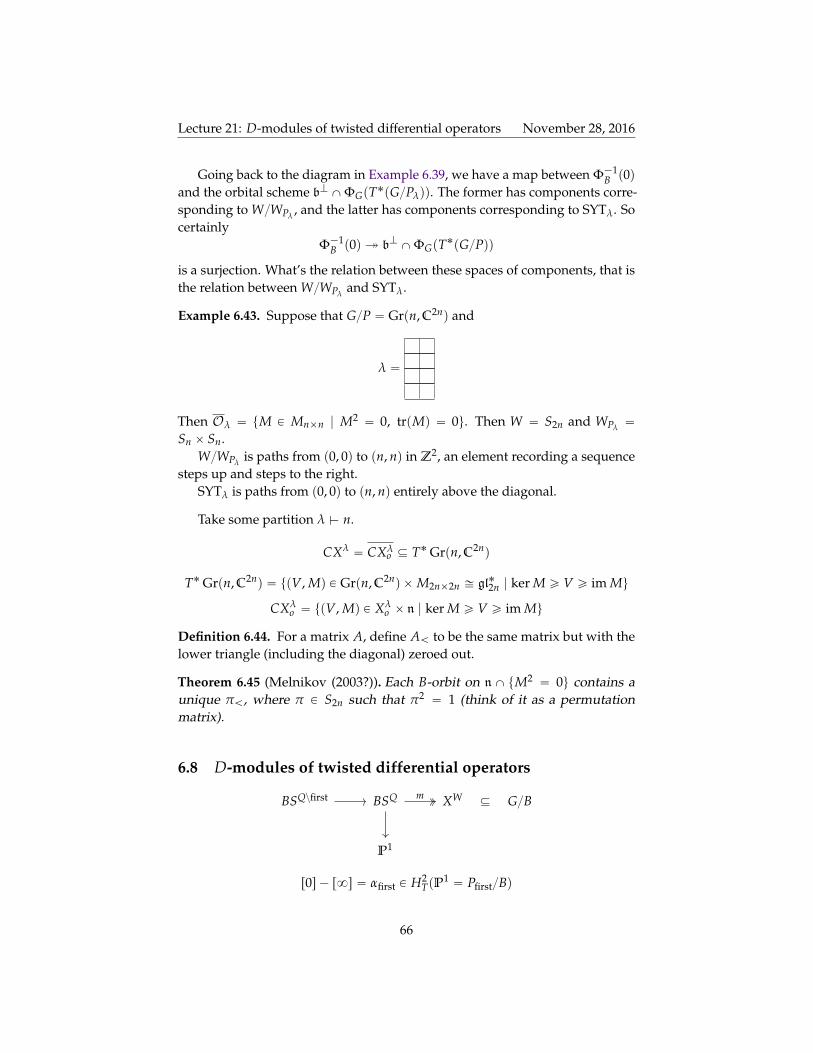
Lecture 21: D-modules of twisted differential operators November 28, 2016
Going back to the diagram in Example 6.39, we have a map between Φ´1B p0q
and the orbital scheme bK XΦGpT˚pGPλqq. The former has components corre-sponding to WWPλ
, and the latter has components corresponding to SYTλ. Socertainly
Φ´1B p0q bK XΦGpT˚pGPqq
is a surjection. What’s the relation between these spaces of components, that isthe relation between WWPλ
and SYTλ.
Example 6.43. Suppose that GP “ Grpn, C2nq and
λ “
Then Oλ “ tM P Mnˆn | M2 “ 0, trpMq “ 0u. Then W “ S2n and WPλ“
Sn ˆ Sn.WWPλ
is paths from p0, 0q to pn, nq in Z2, an element recording a sequencesteps up and steps to the right.
SYTλ is paths from p0, 0q to pn, nq entirely above the diagonal.
Take some partition λ $ n.
CXλ “ CXλo Ď T˚Grpn, C2nq
T˚Grpn, C2nq “ tpV, Mq P Grpn, C2nq ˆM2nˆ2n – gl˚2n | ker M ě V ě im Mu
CXλo “ tpV, Mq P Xλ
o ˆ n | ker M ě V ě im Mu
Definition 6.44. For a matrix A, define Aă to be the same matrix but with thelower triangle (including the diagonal) zeroed out.
Theorem 6.45 (Melnikov (2003?)). Each B-orbit on n X tM2 “ 0u contains aunique πă, where π P S2n such that π2 “ 1 (think of it as a permutationmatrix).
6.8 D-modules of twisted differential operators
BSQzfirst BSQ XW GB
P1
mĎ
r0s ´ r8s “ αfirst P H2TpP
1 “ PfirstBq
66

Lecture 21: D-modules of twisted differential operators November 28, 2016
rBSQzfirsts ´ rαrBSQzfirsts
αfirst“ rBSQs
mÞÝÑ rXws “
1αp1´ rαq
loooomoooon
Bα
rXrαws
This is due to Bernstein-Gelfand-Gelfand in 1973. Notice that B2α “ 0.
Let’s look at rα ` hBα
œ
H˚TpGBqrhs – H˚TˆCˆpT˚pGBqq. We have that
prα ` hBαq2 “ 1.
Recall thatcsmpXw
o q “ÿ
RĎQ
m˚prBSRsq.
This is (combinatorially) equivalent to
prα ` hBαq csmpXwo q “ csmpXrαw
o q.
You can deduce one from the other through some not-so-interesting combina-torics, due to Aluffi-Mihalcea (although they have set h ÞÑ ´1).
G acts on GB from the left, but nothing acts on GB on the right. But GB ishomotopic to GT, which has a map from BT – N.
GB GT BT N
g˚
»
generalorbit
–
However, GB is projective and GT is affine, so they are not equivalent exceptin a topological sense.
However, GT has an action of W on the right, which freely and transitivelypermutes NpTqT ãÑ GT. Also BNpTqT “ rBwTTs. Each of these is closed, ifand only if BwT Ď G is closed, if and only if BzBwT Ď BzG is closed. However,BzBwT is a T-fixed point, so rBwTTs is indeed closed.
Claim that there is a degeneration of GT to T˚pGBq. It’s easy to see thatthere is a degeneration from GT to the nilpotent cone N , given by
G ¨ λ ÞÝÑ limzÑ0
zpG ¨ λq “ limzÑ0
G ¨ pzλq
for λ P t˚reg Ď g˚. The family of these comes from
SpecpFunpgq Ðâ FunpgqG “ FunptqWq
Recall that
T˚pGBq “ tpF, Xq | F flag,X nilpotent preserving Fu
67
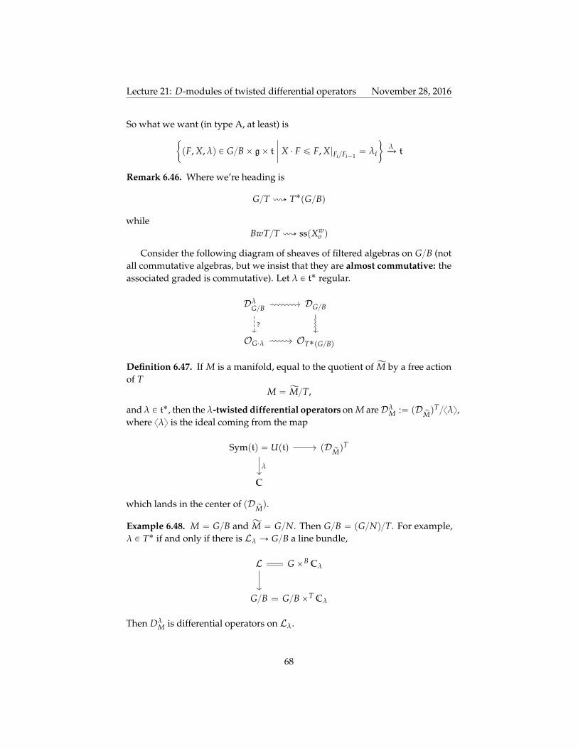
Lecture 21: D-modules of twisted differential operators November 28, 2016
So what we want (in type A, at least) is"
pF, X, λq P GBˆ gˆ t
ˇ
ˇ
ˇ
ˇ
X ¨ F ď F, X|FiFi´1“ λi
*
λÝÑ t
Remark 6.46. Where we’re heading is
GT ù T˚pGBq
whileBwTT ù sspXw
o q
Consider the following diagram of sheaves of filtered algebras on GB (notall commutative algebras, but we insist that they are almost commutative: theassociated graded is commutative). Let λ P t˚ regular.
DλGB DGB
OG¨λ OT˚pGBq
?
Definition 6.47. If M is a manifold, equal to the quotient of ĂM by a free actionof T
M “ ĂMT,
and λ P t˚, then the λ-twisted differential operators on M are DλM :“ pD
rMqTxλy,
where xλy is the ideal coming from the map
Symptq “ Uptq pDrMq
T
C
λ
which lands in the center of pDrMq.
Example 6.48. M “ GB and ĂM “ GN. Then GB “ pGNqT. For example,λ P T˚ if and only if there is Lλ Ñ GB a line bundle,
L GˆB Cλ
GB GBˆT Cλ
Then DλM is differential operators on Lλ.
68

Lecture 22: A bit of silliness November 30, 2016
Example 6.49. We have SLp2qN – C2zt0u, and so DSLp2qN – DC2zt0u. This isgenerated by px, py, ddx, ddy.
T “"„
zz´1
*
pDSLp2qNqT “
B„
pxpy px ddxpy ddy
ddxddy
F
Once you work out the commutation relations among these four operators, thisturns out to be
pDSLp2qNqT – Upglp2qq.
Theorem 6.50 (Beilinson-Bernstein). ΓpDλGBq – Upgqxλy.
The only irreps on which the center of Upgq acts in the same way as it doeson Vλ have high weights W ¨ pλ` ρq ´ ρ.
The easy representations of Upgqxλy are the Verma modules Lpwq :“ Lpwpλ`ρq ´ ρq. If Lpwq ě Lpvq, then wpλ` ρq ´ ρ´ pvpλ` ρq ´ ρq is a sum of positiveroots. Therefore, w ¨ λ´ v ¨ λ is in the root lattice.
But if λ is general, then w ¨ λ´ v ¨ λ being in the root lattice is impossible.Hence, all Lpwq are irreducible.
6.9 A bit of silliness
Let’s say we want to sum some function f over some range r0, bs. Say
Fpbq “bÿ
n“0
f pbq.
What’s the inverse of summing? Differences!
ÿ
“1∆
p∆ f qpaq “ f pa` 1q ´ f paq “ peD ´ 1qp f q
where D is the differential operator, which we have exponentiated. The lastequality above by Talyor series. Therefore,
1∆“
1eD ´ 1
Then as a power series in D, this thing has a pole at D “ 0, whatever that means.So
1∆“
1D
ˆ
DeD ´ 1
˙
“1Dp1` Bernoulli numbersq
69
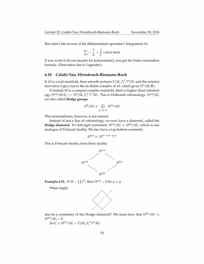
Lecture 22: Calabi-Yau, Hirzebruch-Riemann-Roch November 30, 2016
But what’s the inverse of the differentiation operation? Integration! So
ÿ
“1∆“
ż
`error term
If you work it all out (maybe for polynomials), you get the Euler summationformula. (Derivation due to Legendre.)
6.10 Calabi-Yau, Hirzebruch-Riemann-Roch
If M is a real manifold, then smooth sections ΓpM;Źk T˚Mq and the exterior
derivative d give rise to the de Rahm complex of M, which gives H˚pM; Rq.If instead M is a compact complex manifold, there is higher sheaf cohomol-
ogy Hp,qpM; Cq :“ HqpM;Źp T˚Mq. This is Dolbeault cohomology; Hp,qpMq
are also called Hodge groups.
HkpMq –à
p`q“kHp,qpMq
This isomorphisms, however, is not natural.Instead of just a line of cohomology, we now have a diamond, called the
Hodge diamond. It’s left-right symmetric Hp,qpMq – Hq,ppMq, which is oneanalogue of Poincare duality. We also have a top-bottom symmetry
Hp,q – pHn´p,n´qq˚
This is Poincare duality, from Serre duality.
Hn,n
Hn,0 H0,n
H0,0
Example 6.51. If M “š
Ck, then Hp,q “ 0 for p ‰ q.
When might
also be a symmetry of the Hodge diamond? We must have that H0,npMq –H0,0pMq “ C
So C – H0,npMq “ ΓpM;Źn T˚Mq
70

Lecture 22: Calabi-Yau, Hirzebruch-Riemann-Roch November 30, 2016
Definition 6.52. This condition is called Calabi-Yau.
Example 6.53. If M “ Σg, then the Hodge diamond has dimensions
1
g g
1
So the only Riemann surfaces that are Calabi-Yau are genus 1 (elliptic curves).
Definition 6.54. The Hodge-Poincare Polynomial of M is
HPpx, yq “ÿ
p,qxpyq dim Hp,qpMq
The Euler characteristic is χ “ HPp´1,´1q.
χy :“ HPp´1, yq
is the Hirzebruch χy-genus.
How do we compute χY?
χYpMq “ÿ
p,qp´1qpyq dim HppM;
Źq T˚Mq
“ÿ
qyq
˜
ÿ
pp´1qp dim HppM;
Źq T˚Mq
¸
“ÿ
qyqχpM;
Źq T˚Mq
This is the “K-theory version of integrating the class rŹq T˚Ms”.
Definition 6.55. For a line bundle L on M, the Todd class of L is
TdpLq “ c1pLq1´ e´c1pLq
P H˚pMq.
Definition 6.56. For V Ñ M a complex vector bundle, with Chern roots pLiq,then
TdpVq “ź
TdpLiq.
Theorem 6.57 (Hirzebruch-Riemann-Roch). If LÑ M is a complex line bundleover a compact complex smooth manifold M,
ÿ
i
p´1qi HipM;Lq “ż
Mec1pLq TdpTMq
71

Lecture 22: Calabi-Yau, Hirzebruch-Riemann-Roch November 30, 2016
Example 6.58. M “ CP1 and L “ Opkqwith k ě 0.
k` 1 “ż
CP1p1` krptsqp1` rptsq
Remark 6.59. There’s a version of Hirzebruch-Riemann-Roch that works forgeneral vector bundles V Ñ M, not just line bundles. You have to replace ec1pLq
by the Chern character, which is a map Ch: KpMq Ñ H˚pMq.
We can use Hirzebruch-Riemann-Roch to compute χYpMq. Let TM haveChern roots Li, with c1pLiq “ ri.
Let eq be the q-th elementary symmetric polynomial.
Theorem 6.60 (Hirzebruch signature theorem). Let Li be the Chern roots of TM,with first Chern classes ri. Then
χypMq “ÿ
qyq
ż
MTdpMq eqptexppc1pL˚i qquq
“
ż
MTdpMq
ÿ
qyq eqptexpp´riquq
“
ż
MTdpMq
ÿ
qeqpty expp´riquq
“
ż
M
ź
i
TdpLiqź
i
p1` y expp´riqq
“
ż
M
ź
i
ri1` y expp´riq
1´ expp´riq
At y “ ´1 the integrand is justś
i ri “ epTMq, so this does indeed recover theEuler characteristic.
Fact 6.61. χY extends to an additive function VarpCq Ñ Crys, where VarpCq isthe Grothendieck group of varieties over C, with operation disjoint union. Thensetting y “ ´1 gives usual Euler characteristic.
VarpCq Crys
C
χ
χy
y“´1
Remark 6.62. There is a theory of CSM classes using this! (See arχiv 1303.4454).Say T ãÑ M “ TVp is smooth. Then the χy-csm class is
Ty˚pTq “ p1` yqn TdpŹn T˚Mq
72