Embed Size (px)
Citation preview

Math 439 Course NotesLagrangian Mechanics, Dynamics, and
Control
Andrew D. Lewis
January–April 2003This version: 03/04/2003

ii

This version: 03/04/2003
Preface
These notes deal primarily with the subject of Lagrangian mechanics. Matters related to me-chanics are the dynamics and control of mechanical systems. While dynamics of Lagrangiansystems is a generally well-founded field, control for Lagrangian systems has less of a history.In consequence, the control theory we discuss here is quite elementary, and does not reallytouch upon some of the really challenging aspects of the subject. However, it is hoped thatit will serve to give a flavour of the subject so that people can see if the area is one whichthey’d like to pursue.
Our presentation begins in Chapter 1 with a very general axiomatic treatment of basicNewtonian mechanics. In this chapter we will arrive at some conclusions you may alreadyknow about from your previous experience, but we will also very likely touch upon somethings which you had not previously dealt with, and certainly the presentation is moregeneral and abstract than in a first-time dynamics course. While none of the material inthis chapter is technically hard, the abstraction may be off-putting to some. The hope,however, is that at the end of the day, the generality will bring into focus and demystifysome basic facts about the dynamics of particles and rigid bodies. As far as we know, this isthe first thoroughly Galilean treatment of rigid body dynamics, although Galilean particlemechanics is well-understood.
Lagrangian mechanics is introduced in Chapter 2. When instigating a treatment ofLagrangian mechanics at a not quite introductory level, one has a difficult choice to make;does one use differentiable manifolds or not? The choice made here runs down the middleof the usual, “No, it is far too much machinery,” and, “Yes, the unity of the differentialgeometric approach is exquisite.” The basic concepts associated with differential geometryare introduced in a rather pragmatic manner. The approach would not be one recommendedin a course on the subject, but here serves to motivate the need for using the generality,while providing some idea of the concepts involved. Fortunately, at this level, not overlymany concepts are needed; mainly the notion of a coordinate chart, the notion of a vectorfield, and the notion of a one-form. After the necessary differential geometric introductionsare made, it is very easy to talk about basic mechanics. Indeed, it is possible that theextra time needed to understand the differential geometry is more than made up for whenone gets to looking at the basic concepts of Lagrangian mechanics. All of the principalplayers in Lagrangian mechanics are simple differential geometric objects. Special attentionis given to that class of Lagrangian systems referred to as “simple.” These systems are theones most commonly encountered in physical applications, and so are deserving of specialtreatment. What’s more, they possess an enormous amount of structure, although this isbarely touched upon here. Also in Chapter 2 we talk about forces and constraints. To talkabout control for Lagrangian systems, we must have at hand the notion of a force. We givespecial attention to the notion of a dissipative force, as this is often the predominant effectwhich is unmodelled in a purely Lagrangian system. Constraints are also prevalent in manyapplication areas, and so demand attention. Unfortunately, the handling of constraints inthe literature is often excessively complicated. We try to make things as simple as possible,as the ideas indeed are not all that complicated. While we do not intend these notes tobe a detailed description of Hamiltonian mechanics, we do briefly discuss the link between

iv
Lagrangian Hamiltonian mechanics in Section 2.9. The final topic of discussion in Chapter 2is the matter of symmetries. We give a Noetherian treatment.
Once one uses the material of Chapter 2 to obtain equations of motion, one would like tobe able to say something about how solutions to the equations behave. This is the subjectof Chapter 3. After discussing the matter of existence of solutions to the Euler-Lagrangeequations (a matter which deserves some discussion), we talk about the simplest part ofLagrangian dynamics, dynamics near equilibria. The notion of a linear Lagrangian systemand a linearisation of a nonlinear system are presented, and the stability properties of linearLagrangian systems are explored. The behaviour is nongeneric, and so deserves a treatmentdistinct from that of general linear systems. When one understands linear systems, it isthen possible to discuss stability for nonlinear equilibria. The subtle relationship betweenthe stability of the linearisation and the stability of the nonlinear system is the topic ofSection 3.2. While a general discussion the dynamics of Lagrangian systems with forces isnot realistic, the important class of systems with dissipative forces admits a useful discussion;it is given in Section 3.5. The dynamics of a rigid body is singled out for detailed attentionin Section 3.6. General remarks about simple mechanical systems with no potential energyare also given. These systems are important as they are extremely structure, yet also verychallenging. Very little is really known about the dynamics of systems with constraints. InSection 3.8 we make a few simple remarks on such systems.
In Chapter 4 we deliver our abbreviated discussion of control theory in a Lagrangiansetting. After some generalities, we talk about “robotic control systems,” a generalisationof the kind of system one might find on a shop floor, doing simple tasks. For systemsof this type, intuitive control is possible, since all degrees of freedom are actuated. Forunderactuated systems, a first step towards control is to look at equilibrium points andlinearise. In Section 4.4 we look at the special control structure of linearised Lagrangiansystems, paying special attention to the controllability of the linearisation. For systemswhere linearisations fail to capture the salient features of the control system, one is forcedto look at nonlinear control. This is quite challenging, and we give a terse introduction, andpointers to the literature, in Section 4.5.
Please pass on comments and errors, no matter how trivial. Thank you.
Andrew D. [email protected]
420 Jefferyx32395

This version: 03/04/2003
Table of Contents
1 Newtonian mechanics in Galilean spacetimes 11.1 Galilean spacetime . . . . . . . . . . . . . . . . . . . . . . . . . . . . . . . . 1
1.1.1 Affine spaces . . . . . . . . . . . . . . . . . . . . . . . . . . . . . . . 11.1.2 Time and distance . . . . . . . . . . . . . . . . . . . . . . . . . . . . 51.1.3 Observers . . . . . . . . . . . . . . . . . . . . . . . . . . . . . . . . . 91.1.4 Planar and linear spacetimes . . . . . . . . . . . . . . . . . . . . . . 10
1.2 Galilean mappings and the Galilean transformation group . . . . . . . . . . 121.2.1 Galilean mappings . . . . . . . . . . . . . . . . . . . . . . . . . . . . 121.2.2 The Galilean transformation group . . . . . . . . . . . . . . . . . . . 131.2.3 Subgroups of the Galilean transformation group . . . . . . . . . . . . 151.2.4 Coordinate systems . . . . . . . . . . . . . . . . . . . . . . . . . . . 171.2.5 Coordinate systems and observers . . . . . . . . . . . . . . . . . . . 19
1.3 Particle mechanics . . . . . . . . . . . . . . . . . . . . . . . . . . . . . . . . 211.3.1 World lines . . . . . . . . . . . . . . . . . . . . . . . . . . . . . . . . 211.3.2 Interpretation of Newton’s Laws for particle motion . . . . . . . . . 23
1.4 Rigid motions in Galilean spacetimes . . . . . . . . . . . . . . . . . . . . . . 251.4.1 Isometries . . . . . . . . . . . . . . . . . . . . . . . . . . . . . . . . . 251.4.2 Rigid motions . . . . . . . . . . . . . . . . . . . . . . . . . . . . . . 271.4.3 Rigid motions and relative motion . . . . . . . . . . . . . . . . . . . 301.4.4 Spatial velocities . . . . . . . . . . . . . . . . . . . . . . . . . . . . . 301.4.5 Body velocities . . . . . . . . . . . . . . . . . . . . . . . . . . . . . . 331.4.6 Planar rigid motions . . . . . . . . . . . . . . . . . . . . . . . . . . . 36
1.5 Rigid bodies . . . . . . . . . . . . . . . . . . . . . . . . . . . . . . . . . . . 371.5.1 Definitions . . . . . . . . . . . . . . . . . . . . . . . . . . . . . . . . 371.5.2 The inertia tensor . . . . . . . . . . . . . . . . . . . . . . . . . . . . 401.5.3 Eigenvalues of the inertia tensor . . . . . . . . . . . . . . . . . . . . 411.5.4 Examples of inertia tensors . . . . . . . . . . . . . . . . . . . . . . . 45
1.6 Dynamics of rigid bodies . . . . . . . . . . . . . . . . . . . . . . . . . . . . 461.6.1 Spatial momenta . . . . . . . . . . . . . . . . . . . . . . . . . . . . . 471.6.2 Body momenta . . . . . . . . . . . . . . . . . . . . . . . . . . . . . . 491.6.3 Conservation laws . . . . . . . . . . . . . . . . . . . . . . . . . . . . 501.6.4 The Euler equations in Galilean spacetimes . . . . . . . . . . . . . . 521.6.5 Solutions of the Galilean Euler equations . . . . . . . . . . . . . . . 55
1.7 Forces on rigid bodies . . . . . . . . . . . . . . . . . . . . . . . . . . . . . . 561.8 The status of the Newtonian world view . . . . . . . . . . . . . . . . . . . . 57
2 Lagrangian mechanics 612.1 Configuration spaces and coordinates . . . . . . . . . . . . . . . . . . . . . . 61
2.1.1 Configuration spaces . . . . . . . . . . . . . . . . . . . . . . . . . . . 622.1.2 Coordinates . . . . . . . . . . . . . . . . . . . . . . . . . . . . . . . . 642.1.3 Functions and curves . . . . . . . . . . . . . . . . . . . . . . . . . . . 69
2.2 Vector fields, one-forms, and Riemannian metrics . . . . . . . . . . . . . . . 69

vi
2.2.1 Tangent vectors, tangent spaces, and the tangent bundle . . . . . . . 692.2.2 Vector fields . . . . . . . . . . . . . . . . . . . . . . . . . . . . . . . 742.2.3 One-forms . . . . . . . . . . . . . . . . . . . . . . . . . . . . . . . . 772.2.4 Riemannian metrics . . . . . . . . . . . . . . . . . . . . . . . . . . . 82
2.3 A variational principle . . . . . . . . . . . . . . . . . . . . . . . . . . . . . . 852.3.1 Lagrangians . . . . . . . . . . . . . . . . . . . . . . . . . . . . . . . . 852.3.2 Variations . . . . . . . . . . . . . . . . . . . . . . . . . . . . . . . . . 862.3.3 Statement of the variational problem and Euler’s necessary condition 862.3.4 The Euler-Lagrange equations and changes of coordinate . . . . . . . 89
2.4 Simple mechanical systems . . . . . . . . . . . . . . . . . . . . . . . . . . . 912.4.1 Kinetic energy . . . . . . . . . . . . . . . . . . . . . . . . . . . . . . 912.4.2 Potential energy . . . . . . . . . . . . . . . . . . . . . . . . . . . . . 922.4.3 The Euler-Lagrange equations for simple mechanical systems . . . . 932.4.4 Affine connections . . . . . . . . . . . . . . . . . . . . . . . . . . . . 96
2.5 Forces in Lagrangian mechanics . . . . . . . . . . . . . . . . . . . . . . . . . 992.5.1 The Lagrange-d’Alembert principle . . . . . . . . . . . . . . . . . . . 992.5.2 Potential forces . . . . . . . . . . . . . . . . . . . . . . . . . . . . . . 1012.5.3 Dissipative forces . . . . . . . . . . . . . . . . . . . . . . . . . . . . . 1032.5.4 Forces for simple mechanical systems . . . . . . . . . . . . . . . . . . 107
2.6 Constraints in mechanics . . . . . . . . . . . . . . . . . . . . . . . . . . . . 1082.6.1 Definitions . . . . . . . . . . . . . . . . . . . . . . . . . . . . . . . . 1082.6.2 Holonomic and nonholonomic constraints . . . . . . . . . . . . . . . 1102.6.3 The Euler-Lagrange equations in the presence of constraints . . . . . 1152.6.4 Simple mechanical systems with constraints . . . . . . . . . . . . . . 1182.6.5 The Euler-Lagrange equations for holonomic constraints . . . . . . . 121
2.7 Newton’s equations and the Euler-Lagrange equations . . . . . . . . . . . . 1242.7.1 Lagrangian mechanics for a single particle . . . . . . . . . . . . . . . 1242.7.2 Lagrangian mechanics for multi-particle and multi-rigid body systems 126
2.8 Euler’s equations and the Euler-Lagrange equations . . . . . . . . . . . . . . 1282.8.1 Lagrangian mechanics for a rigid body . . . . . . . . . . . . . . . . . 1292.8.2 A modified variational principle . . . . . . . . . . . . . . . . . . . . . 130
2.9 Hamilton’s equations . . . . . . . . . . . . . . . . . . . . . . . . . . . . . . . 1332.10 Conservation laws . . . . . . . . . . . . . . . . . . . . . . . . . . . . . . . . 136
3 Lagrangian dynamics 1493.1 The Euler-Lagrange equations and differential equations . . . . . . . . . . . 1493.2 Linearisations of Lagrangian systems . . . . . . . . . . . . . . . . . . . . . . 151
3.2.1 Linear Lagrangian systems . . . . . . . . . . . . . . . . . . . . . . . 1513.2.2 Equilibria for Lagrangian systems . . . . . . . . . . . . . . . . . . . 157
3.3 Stability of Lagrangian equilibria . . . . . . . . . . . . . . . . . . . . . . . . 1603.3.1 Equilibria for simple mechanical systems . . . . . . . . . . . . . . . . 165
3.4 The dynamics of one degree of freedom systems . . . . . . . . . . . . . . . . 1703.4.1 General one degree of freedom systems . . . . . . . . . . . . . . . . . 1713.4.2 Simple mechanical systems with one degree of freedom . . . . . . . . 176
3.5 Lagrangian systems with dissipative forces . . . . . . . . . . . . . . . . . . . 1813.5.1 The LaSalle Invariance Principle for dissipative systems . . . . . . . 1813.5.2 Single degree of freedom case studies . . . . . . . . . . . . . . . . . . 185
3.6 Rigid body dynamics . . . . . . . . . . . . . . . . . . . . . . . . . . . . . . . 187

vii
3.6.1 Conservation laws and their implications . . . . . . . . . . . . . . . . 1873.6.2 The evolution of body angular momentum . . . . . . . . . . . . . . . 1903.6.3 Poinsot’s description of a rigid body motion . . . . . . . . . . . . . . 194
3.7 Geodesic motion . . . . . . . . . . . . . . . . . . . . . . . . . . . . . . . . . 1953.7.1 Basic facts about geodesic motion . . . . . . . . . . . . . . . . . . . 1953.7.2 The Jacobi metric . . . . . . . . . . . . . . . . . . . . . . . . . . . . 197
3.8 The dynamics of constrained systems . . . . . . . . . . . . . . . . . . . . . . 1993.8.1 Existence of solutions for constrained systems . . . . . . . . . . . . . 1993.8.2 Some general observations . . . . . . . . . . . . . . . . . . . . . . . . 2023.8.3 Constrained simple mechanical systems . . . . . . . . . . . . . . . . 202
4 An introduction to control theory for Lagrangian systems 2114.1 The notion of a Lagrangian control system . . . . . . . . . . . . . . . . . . . 2114.2 “Robot control” . . . . . . . . . . . . . . . . . . . . . . . . . . . . . . . . . 212
4.2.1 The equations of motion for a robotic control system . . . . . . . . . 2134.2.2 Feedback linearisation for robotic systems . . . . . . . . . . . . . . . 2154.2.3 PD control . . . . . . . . . . . . . . . . . . . . . . . . . . . . . . . . 216
4.3 Passivity methods . . . . . . . . . . . . . . . . . . . . . . . . . . . . . . . . 2174.4 Linearisation of Lagrangian control systems . . . . . . . . . . . . . . . . . . 217
4.4.1 The linearised system . . . . . . . . . . . . . . . . . . . . . . . . . . 2174.4.2 Controllability of the linearised system . . . . . . . . . . . . . . . . . 2184.4.3 On the validity of the linearised system . . . . . . . . . . . . . . . . 224
4.5 Control when linearisation does not work . . . . . . . . . . . . . . . . . . . 2244.5.1 Driftless nonlinear control systems . . . . . . . . . . . . . . . . . . . 2244.5.2 Affine connection control systems . . . . . . . . . . . . . . . . . . . . 2264.5.3 Mechanical systems which are “reducible” to driftless systems . . . . 2274.5.4 Kinematically controllable systems . . . . . . . . . . . . . . . . . . . 229
A Linear algebra 235A.1 Vector spaces . . . . . . . . . . . . . . . . . . . . . . . . . . . . . . . . . . . 235A.2 Dual spaces . . . . . . . . . . . . . . . . . . . . . . . . . . . . . . . . . . . . 237A.3 Bilinear forms . . . . . . . . . . . . . . . . . . . . . . . . . . . . . . . . . . 238A.4 Inner products . . . . . . . . . . . . . . . . . . . . . . . . . . . . . . . . . . 239A.5 Changes of basis . . . . . . . . . . . . . . . . . . . . . . . . . . . . . . . . . 240
B Differential calculus 243B.1 The topology of Euclidean space . . . . . . . . . . . . . . . . . . . . . . . . 243B.2 Mappings between Euclidean spaces . . . . . . . . . . . . . . . . . . . . . . 244B.3 Critical points of R-valued functions . . . . . . . . . . . . . . . . . . . . . . 244
C Ordinary differential equations 247C.1 Linear ordinary differential equations . . . . . . . . . . . . . . . . . . . . . . 247C.2 Fixed points for ordinary differential equations . . . . . . . . . . . . . . . . 249
D Some measure theory 253

viii

This version: 03/04/2003
Chapter 1
Newtonian mechanics in Galilean spacetimes
One hears the term relativity typically in relation to Einstein and his two theories of rel-ativity, the special and the general theories. While the Einstein’s general theory of relativitycertainly supplants Newtonian mechanics as an accurate model of the macroscopic world, itis still the case that Newtonian mechanics is sufficiently descriptive, and easier to use, thanEinstein’s theory. Newtonian mechanics also comes with its form of relativity, and in thischapter we will investigate how it binds together the spacetime of the Newtonian world. Wewill see how the consequences of this affect the dynamics of a Newtonian system. On theroad to these lofty objectives, we will recover many of the more prosaic elements of dynamicsthat often form the totality of the subject at the undergraduate level.
1.1 Galilean spacetime
Mechanics as envisioned first by Galileo Galilei (1564–1642) and Isaac Newton (1643–1727), and later by Leonhard Euler (1707–1783), Joseph-Louis Lagrange (1736–1813), Pierre-Simon Laplace (1749–1827), etc., take place in a Galilean spacetime. By this we mean thatwhen talking about Newtonian mechanics we should have in mind a particular model forphysical space in which our objects are moving, and means to measure how long an eventtakes. Some of what we say in this section may be found in the first chapter of [Arnol’d 1989]and in the paper [Artz 1981]. The presentation here might seem a bit pretentious, but theidea is to emphasise that Newtonian mechanics is a axio-deductive system, with all theadvantages and disadvantages therein.
1.1.1 Affine spaces In this section we introduce a concept that bears some resem-blance to that of a vector space, but is different in a way that is perhaps a bit subtle. Anaffine space may be thought of as a vector space “without an origin.” Thus it makes senseonly to consider the “difference” of two elements of an affine space as being a vector. Theelements themselves are not to be regarded as vectors. For a more thorough discussion ofaffine spaces and affine geometry we refer the reader to the relevant sections of [Berger 1987].
1.1.1 Definition Let V be a R-vector space. An affine space modelled on V is a set A anda map φ : V × A→ A with the properties
AS1. for every x, y ∈ A there exists v ∈ V so that y = φ(v, x),
AS2. φ(v, x) = x for every x ∈ A implies that v = 0,
AS3. φ(0, x) = x, and
AS4. φ(u+ v, x) = φ(u, φ(v, x)).

2 1 Newtonian mechanics in Galilean spacetimes 03/04/2003
We shall now cease to use the map φ and instead use the more suggestive notation φ(v, x) =v + x. By properties AS1 and AS2, if x, y ∈ A then there exists a unique v ∈ V such thatv + x = y. In this case we shall denote v = y − x. Note that the minus sign is simplynotation; we have not really defined “subtraction” in A! The idea is that to any two pointsin A we may assign a unique vector in V and we notationally write this as the differencebetween the two elements. All this leads to the following result.
1.1.2 Proposition Let A be a R-affine space modelled on V. For fixed x ∈ A define vectoraddition on A by
y1 + y2 = ((y1 − x) + (y2 − x)) + x
(note y1 − x, y2 − x ∈ V) and scalar multiplication on A by
ay = (a(y − x)) + x
(note that y − x ∈ V). These operations make a A a R-vector space and y 7→ y − x is anisomorphism of this R-vector space with V.
This result is easily proved once all the symbols are properly understood (see Exercise E1.1).The gist of the matter is that for fixed x ∈ A we can make A a R-vector space in a naturalway, but this does depend on the choice of x. One can think of x as being the “origin” ofthis vector space. Let us denote this vector space by Ax to emphasise its dependence on x.
A subset B of a R-affine space A modelled on V is an affine subspace if there is asubspace U of V with the property that y − x ∈ U for every x, y ∈ B. That is to say,B is an affine subspace if all of its points “differ” by some subspace of V . In this case Bis itself a R-affine space modelled on U . The following result further characterises affinesubspaces. Its proof is a simple exercise in using the definitions and we leave it to the reader(see Exercise E1.2).
1.1.3 Proposition Let A be a R-affine space modelled on the R-vector space V and let B ⊂ A.The following are equivalent:
(i) B is an affine subspace of A;
(ii) there exists a subspace U of V so that for some fixed x ∈ B, B = u + x | u ∈ U;(iii) if x ∈ B then y − x | y ∈ B ⊂ V is a subspace.
1.1.4 Example A R-vector space V is a R-affine space modelled on itself. To emphasise thedifference between V the R-affine space and V the R-vector space we denote points in theformer by x, y and points in the latter by u, v. We define v + x (the affine sum) to be v + x(the vector space sum). If x, y ∈ V then y−x (the affine difference) is simply given by y−x(the vector space difference). Figure 1.1 tells the story. The essential, and perhaps hard tograsp, point is that u and v are not to be regarded as vectors, but simply as points.
An affine subspace of the affine space V is of the form x+U (affine sum) for some x ∈ Vand a subspace U of V . Thus an affine subspace is a “translated” subspace of V . Note thatin this example this means that affine subspaces do not have to contain 0 ∈ V—affine spaceshave no origin.
Maps between vector spaces that preserve the vector space structure are called linearmaps. There is a similar class of maps between affine spaces. If A and B are R-affine spacesmodelled on V and U , respectively, a map f : A→ B is a R-affine map if for each x ∈ A,f is a R-linear map between the R-vector spaces Ax and Bf(x).

03/04/2003 1.1 Galilean spacetime 3
x
y
y − x
y − x
the vector space V the affine space V
Figure 1.1 A vector space can be thought of as an affine space
1.1.5 Example (1.1.4 cont’d) Let V and U be R-vector spaces that we regard as R-affinespaces. We claim that every R-affine map is of the form f : x 7→ Ax + y0 where A is aR-linear map and y0 ∈ U is fixed.
First let us show that a map of this form is a R-affine map. Let x1, x2 ∈ Ax for somex ∈ V . Then we compute
f(x1 + x2) = f((x1 − x) + (x2 − x) + x)
= f(x1 + x2 − x)
= A(x1 + x2 − x) + y0,
and
f(x1) + f(x2) =(((Ax1 + y0)− (Ax+ y0)) + ((Ax2 + y0)− (Ax+ y0))
)+ Ax+ y0
= A(x1 + x2 − x) + y0
showing that f(x1 +x2) = f(x1)+ f(x2). The above computations will look incorrect unlessyou realise that the +-sign is being employed in two different ways. That is, when we writef(x1 + x2) and f(x1) + f(x2), addition is in Vx and Uf(x), respectively. Similarly one showthat f(ax1) = af(x1) which demonstrates that f in a R-affine map.
Now we show that any R-affine map must have the form given for f . Let 0 ∈ V be thezero vector. For x1, x2 ∈ V0 we have
f(x1 + x2) = f((x1 − 0) + (x2 − 0) + 0) = f(x1 + x2),
where the +-sign on the far left is addition in V0 and on the far right is addition in V .Because f : V0 → Uf(0) is R-linear, we also have
f(x1 + x2) = f(x1) + f(x2) = (f(x1)− f(0)) + (f(x2)− f(0)) + f(0) = f(x1) + f(x2)− f(0).
Again, on the far left the +-sign is for Uf(0) and on the far right is for U . Thus we haveshown that, for regular vector addition in V and U we must have
f(x1 + x2) = f(x1) + f(x2)− f(0). (1.1)
Similarly, using linearity of f : V0 → Uf(0) under scalar multiplication we get
f(ax1) = a(f(x1)− f(0)) + f(0), (1.2)

4 1 Newtonian mechanics in Galilean spacetimes 03/04/2003
for a ∈ R and x1 ∈ Vx. Here, vector addition is in V and U . Together (1.1) and (1.2)imply that the map V ∈ x 7→ f(x) − f(0) ∈ U is R-linear. This means that there existsA ∈ L(V ;U) so that f(x)− f(0) = Ax. After taking y0 = f(0) our claim now follows.
If A and B are R-affine spaces modelled on R-vector spaces V and U , respectively, thenwe may define a R-linear map fV : V → U as follows. Given x0 ∈ A let Ax0 and Bf(x0) be thecorresponding vector spaces as described in Proposition 1.1.2. Recall that Ax0 is isomorphicto V with the isomorphism x 7→ x− x0 and Bf(x0) is isomorphic to U with the isomorphismy 7→ y − f(x0). Let us denote these isomorphisms by gx0 : Ax0 → V and gf(x0) : Bf(x0) → U ,respectively. We then define
fV (v) = gf(x0) f g−1x0
(v). (1.3)
It only remains to check that this definition does not depend on x0 (see Exercise E1.5).
1.1.6 Example (Example 1.1.4 cont’d) Recall that if V is a R-vector space, then it is an R-affine space modelled on itself (Example 1.1.4). Also recall that if U is another R-vectorspace that we also think of as a R-affine space, then an affine map from V to U looks likef(x) = Ax+ y0 for a R linear map A and for some y0 ∈ U (Example 1.1.5).
Let’s see what fV looks like in such a case. Well, we can certainly guess what it shouldbe! But let’s work through the definition to see how it works. Pick some x0 ∈ V so that
gx0(x) = x− x0, gf(x0)(y) = y − f(x0) = y − Ax0 − y0.
We then see thatg−1
x0(v) = v − x0.
Now apply the definition (1.3):
fV (v) = gf(x0) f g−1x0
(v)
= gf(x0) f(v + x0)
= gf(x0)(A(v + x0) + y0)
= A(v + x0) + y0 − Ax0 − y0
= Av.
Therefore we have laboriously derived what can be the only possible answer: fV = A!
Finally, let us talk briefly about convexity, referring to [Berger 1987] for more details.We shall really only refer to this material once (see Lemma 1.5.2), so this material can beskimmed liberally if one is so inclined. A subset C of an affine space A is convex if for anytwo points x, y ∈ C the set
`x,y = t(y − x) + x | t ∈ [0, 1]
is contained in C. This simply means that a set is convex if the line connecting any twopoints in the set remains within the set. For a given, not necessarily convex, subset S of Awe define
co(S) =⋂C
C is a convex set containing S
to be the convex hull of S. Thus co(S) is the smallest convex set containing S. Forexample, the convex hull of a set of two distinct points S = x, y will be the line `x,y, and

03/04/2003 1.1 Galilean spacetime 5
the convex hull of three non-collinear points S = x, y, z will be the triangle with the pointsas vertices.
The following characterisation of a convex set will be useful. We refer to Appendix B forthe definition of relative interior.
1.1.7 Proposition Let A be an affine space modelled on V and let C ( A be a convex set. Ifx ∈ A is not in the relative interior of C then there exists λ ∈ V∗ so that C ⊂ Vλ + x where
Vλ = v ∈ V | λ(v) > 0 .
The idea is simply that a convex set can be separated from its complement by a hyperplaneas shown in Figure 1.2. The vector λ ∈ V ∗ can be thought of as being “orthogonal” to the
C
λ
Vλ
x
Figure 1.2 A hyperplane separating a convex set from its comple-ment
hyperplane Vλ.
1.1.2 Time and distance We begin by giving the basic definition of a Galilean space-time, and by providing meaning to intuitive notions of time and distance.
1.1.8 Definition A Galilean spacetime is a quadruple G = (E , V, g, τ) where
GSp1. V is a 4-dimensional vector space,
GSp2. τ : V → R is a surjective linear map called the time map,
GSp3. g is an inner product on ker(τ), and
GSp4. E is an affine space modelled on V .
Points in E are called events—thus E is a model for the spatio-temporal world of Newtonianmechanics. With the time map we may measure the time between two events x1, x2 ∈ Eas τ(x2 − x1) (noting that x1 − x2 ∈ V ). Note, however, that it does not make sense totalk about the “time” of a particular event x ∈ E , at least not in the way you are perhaps

6 1 Newtonian mechanics in Galilean spacetimes 03/04/2003
tempted to do. If x1 and x2 are events for which τ(x2 − x1) = 0 then we say x1 and x2 aresimultaneous .
Using the lemma, we may define the distance between simultaneous events x1, x2 ∈ Eto be
√g(x2 − x1, x2 − x1). Note that this method for defining distance does not allow us
to measure distance between events that are not simultaneous. In particular, it does notmake sense to talk about two non-simultaneous events as occuring in the same place (i.e., asseparated by zero distance). The picture one should have in mind for a Galilean spacetime isof it being a union of simultaneous events, nicely stacked together as depicted in Figure 1.3.That one cannot measure distance between non-simultaneous events reflects there being no
Figure 1.3 Vertical dashed lines represent simultaneous events
natural direction transverse to the stratification by simultaneous events.Also associated with simultaneity is the collection of simultaneous events. For a given
Galilean spacetime G = (E , V, g, τ) we denote by
IG = S ⊂ E | S is a collection of simultaneous events
the collection of all simultaneous events. We shall frequently denote a point in IG by s, butkeep in mind that when we do this, s is actually a collection of simultaneous events. We willdenote by πG : E → IG the map that assigns to x ∈ E the set of points simultaneous with x.Therefore, if s0 = πG (x0) then the set
π−1G (s0) = x ∈ E | πG (x) = s0
is simply a collection of simultaneous events. Given some s ∈ IG , we denote by E (s) thoseevents x for which πG (x) = s.
1.1.9 Lemma For each s ∈ IG , E (s) is a 3-dimensional affine space modelled on ker(τ).
Proof The affine action of ker(τ) on E (s) is that obtained by restricting the affine action ofV on E . So first we must show this restriction to be well-defined. That is, given v ∈ ker(τ) weneed to show that v+x ∈ E (s) for every x ∈ E (s). If x ∈ E (s) then τ((v+x)−x) = τ(v) = 0which means that v+x ∈ E (s) as claimed. The only non-trivial part of proving the restriction

03/04/2003 1.1 Galilean spacetime 7
defines an affine structure is showing that the action satisfies part AS1 of the definition ofan affine space. However, this follows since, thought of as a R-vector space (with somex0 ∈ E (s) as origin), E (s) is a 3-dimensional subspace of E . Indeed, it is the kernel of thelinear map x 7→ τ(x− x0) that has rank 1.
Just as a single set of simultaneous events is an affine space, so too is the set of allsimultaneous events.
1.1.10 Lemma IG is a 1-dimensional affine space modelled on R.
Proof The affine action of R on IG is defined as follows. For t ∈ R and s1 ∈ IG , we definet+ s1 to be s2 = πG (x2) where τ(x2− x1) = t for some x1 ∈ E (s1) and x2 ∈ E (s2). We needto show that this definition is well-defined, i.e., does not depend on the choices made for x1
and x2. So take x′1 ∈ E (s1) and x′2 ∈ E (s2). Since x′1 ∈ E (s1) we have x′1− x1 = v1 ∈ ker(τ)and similarly x′2 − x2 = v2 ∈ ker(τ). Therefore
τ(x′2 − x′1) = τ((v2 + x2)− (v1 + x1)) = τ((v2 − v1) + (x2 − x1)) = τ(x2 − x1),
where we have used associativity of affine addition. Therefore, the condition that τ(x2−x1) =t does not depend on the choice of x1 and x2.
One should think of IG as being the set of “times” for a Galilean spacetime, but it isan affine space, reflecting the fact that we do not have a distinguished origin for time (seeFigure 1.4). Following Artz [1981], we call IG the set of instants in the Galilean spacetime
E (s)
s
Figure 1.4 The set of instants IG
G , the idea being that each of the sets E (s) of simultaneous events defines an instant.The Galilean structure also allows for the use of the set
VG = v ∈ V | τ(v) = 1 .

8 1 Newtonian mechanics in Galilean spacetimes 03/04/2003
The interpretation of this set is, as we shall see, that of a Galilean invariant velocity. Let uspostpone this until later, and for now merely observe the following.
1.1.11 Lemma VG is a 3-dimensional affine space modelled on ker(τ).
Proof Since τ is surjective, VG is nonempty. We claim that if u0 ∈ VG then
VG = u0 + v | v ∈ ker(τ) .
Indeed, let u ∈ VG . Then τ(u− u0) = τ(u)− τ(u0) = 1− 1 = 0. Therefore u− u0 ∈ ker(τ)so that
VG ⊂ u0 + v | v ∈ ker(τ) . (1.4)
Conversely, if u ∈ u0 + v | v ∈ ker(τ) then there exists v ∈ ker(τ) so that u = u0 + v.Thus τ(u) = τ(u0 + v) = τ(u0) = 1, proving the opposite inclusion.
With this in mind, we define the affine action of ker(τ) on VG by v + u = v + u, i.e., thenatural addition in V . That this is well-defined follows from the equality (1.4).
To summarise, given a Galilean spacetime G = (E , V, g, τ), there are the following objectsthat one may associated with it:
1. the 3-dimensional vector space ker(τ) that, as we shall see, is where angular velocitiesand acceleration naturally live;
2. the 1-dimensional affine space IG of instants;
3. for each s ∈ IG , the 3-dimensional affine space E (s) of events simultaneous with E ;
4. the 3-dimensional affine space VG of “Galilean velocities.”
We shall be encountering these objects continually throughout our development of mechanicsin Galilean spacetimes.
When one think of Galilean spacetime, one often has in mind a particular example.
1.1.12 Example We let E = R3×R ' R4 which is an affine space modelled on V = R4 in thenatural way (see Example 1.1.4). The time map we use is given by τcan(v
1, v2, v3, v4) = v4.Thus
ker(τcan) =
(v1, v2, v3, v4) ∈ V∣∣ v4 = 0
is naturally identified with R3, and we choose for g the standard inner product on R3 thatwe denote by gcan. We shall call this particular Galilean spacetime the standard Galileanspacetime .
(Notice that we write the coordinates (v1, v2, v3, v4) with superscripts . This will doubtlesscause some annoyance, but as we shall see in Section 2.1, there is some rhyme and reasonbehind this.)
Given two events ((x1, x2, x3), s) and ((y1, y2, y3), t) one readily verifies that the timebetween these events is t− s. The distance between simultaneous events ((x1, x2, x3), t) and((y1, y2, y3), t) is then√
(y1 − x1)2 + (y2 − x2)2 − (y3 − x3)2 = ‖y − x‖
where ‖·‖ is thus the standard norm on R3.For an event x = ((x1
0, x20, x
30), t), the set of events simultaneous with x is
E (t) =
((x1, x2, x3), t)∣∣ xi = xi
0, i = 1, 2, 3.

03/04/2003 1.1 Galilean spacetime 9
The instant associated with x is naturally identified with t ∈ R, and this gives us a simpleidentification of IG with R. We also see that
VG =
(v1, v2, v3, v4) ∈ V∣∣ v4 = 1
,
and so we clearly have VG = (0, 0, 0, 1) + ker(τcan).
1.1.3 Observers An observer is to be thought of intuitively as someone who is presentat each instant, and whose world behaves as according to the laws of motion (about which,more later). Such an observer should be moving at a uniform velocity. Note that in aGalilean spacetime, the notion of “stationary” makes no sense. We can be precise about anobserver as follows. An observer in a Galilean spacetime G = (E , V, g, τ) is a 1-dimensionalaffine subspace O of E with the property that O ( E (s) for any s ∈ IG . That is, the affinesubspace O should not consist wholly of simultaneous events. There are some immediateimplications of this definition.
1.1.13 Proposition If O is an observer in a Galilean spacetime G = (E ,V, g, τ) then for eachs ∈ IG there exists a unique point x ∈ O ∩ E (s).
Proof It suffices to prove the proposition for the canonical Galilean spacetime. (The reasonfor this is that, as we shall see in Section 1.2.4, a “coordinate system” has the propertythat it preserves simultaneous events.) We may also suppose that (0, 0) ∈ O. With thesesimplifications, the observer is then a 1-dimensional subspace passing through the origin inR3 ×R. What’s more, since O is not contained in a set of simultaneous events, there existsa point of the form (x, t) in O where t 6= 0. Since O is a subspace, this means that allpoints (ax, at) must also be in O for any a ∈ R. This shows that O ∩ E (s) is nonempty forevery s ∈ IG . That O ∩ E (s) contains only one point follows since 1-dimensionality of Oensures that the vector (x, t) is a basis for O. Therefore any two distinct points (a1x, a1t)and (a2x, a2t) in O will not be simultaneous.
We shall denote by Os the unique point in the intersection O ∩ E (s).This means that an observer, as we have defined it, does indeed have the property of
sitting at a place, and only one place, at each instant of time (see Figure 1.5). However,the observer should also somehow have the property of having a uniform velocity. Let ussee how this plays out with our definition. Given an observer O in a Galilean spacetimeG = (E , V, g, τ), let U ⊂ V be the 1-dimensional subspace upon which O is modelled. Therethen exists a unique vector vO ∈ U with the property that τ(vO) = 1. We call vO theGalilean velocity of the observer O. Again, it makes no sense to say that an observer isstationary, and this is why we must use the Galilean velocity.
An observer O in a Galilean spacetime G = (E , V, g, τ) with its Galilean velocity vO
enables us to resolve other Galilean velocities into regular velocities. More generally, itallows us to resolve vectors in v ∈ V into a spatial component to go along with theirtemporal component τ(v). This is done by defining a linear map PO : V → ker(τ) by
PO(v) = v − (τ(v))vO .
(Note that τ(v− (τ(v))vO) = τ(v)− τ(v)τ(vO) = 0 so PO(v) in indeed in ker(τ).) FollowingArtz [1981], we call PO the O-spatial projection . For Galilean velocities, i.e., when v ∈VG ⊂ V , PO(v) can be thought of as the velocity of v relative to the observer’s Galileanvelocity vO . The following trivial result says just this.

10 1 Newtonian mechanics in Galilean spacetimes 03/04/2003
O
O ∩ E (s)
E (s)
Figure 1.5 The idea of an observer
1.1.14 Lemma If O is an observer in a Galilean spacetime G = (E ,V, g, τ) and if v ∈ VG ,then v = vO + PO(v).
Proof This follows since τ(v) = 1 when v ∈ VG .
The following is a very simple example of an observer in the canonical Galilean spacetime,and represents the observer one unthinkingly chooses in this case.
1.1.15 Example We let Gcan = (R3 × R,R4, gcan, τcan) be the canonical Galilean spacetime.The canonical observer is defined by
Ocan = (0, t) | t ∈ R .
Thus the canonical observer sits at the origin in each set of simultaneous events.
1.1.4 Planar and linear spacetimes When dealing with systems that move in a planeor a line, things simplify to an enormous extent. But how does one talk of planar or linearsystems in the context of Galilean spacetimes? The idea is quite simple.
1.1.16 Definition Let G = (E , V, g, τ) be a Galilean spacetime. A subset F of E is a sub-spacetime if there exists a nontrivial subspace U of V with the property that
Gsub1. F is an affine subspace of E modelled on U and
Gsub2. τ |U : U → R is surjective.
The dimension of the sub-spacetime F is the dimension of the subspace U .
Let us denote Uτ = U ∩ ker(τ). The idea then is simply that we obtain a “new” spacetimeH = (F , U, g|Uτ , τ |U) of smaller dimension. We shall often refer to H so defined as thesub-spacetime interchangeably with F . The idea of condition Gsub2 is that the time mapshould still be well defined. If we were to choose F so that its model subspace U were asubset of ker(τ) then we would lose our notion of time.

03/04/2003 1.1 Galilean spacetime 11
1.1.17 Examples If (E = R3×R, V = R4, gcan, τcan) is the standard Galilean spacetime, thenwe may choose “natural” planar and linear sub-spacetimes as follows.
1. For the planar sub-spacetime, take
F3 =
((x, y, z), t) ∈ R3 × R∣∣ z = 0
,
andU3 =
(u, v, w, s) ∈ R4
∣∣ w = 0.
Therefore, F3 looks like R2 × R and we may use coordinates ((x, y), t) as coordinates.Similarly U3 looks like R3 and we may use (u, v, s) as coordinates. With these coordinateswe have
ker(τcan|U3) =
(u, v, s) ∈ R3∣∣ s = 0
,
so that gcan restricted to ker(τcan) is the standard inner product on R2 with coordinates(u, v). One then checks that with the affine structure as defined in Example 1.1.12, H3 =(F3, U3, gcan|U3,τcan , τcan|U3) is a 3-dimensional Galilean sub-spacetime of the canonicalGalilean spacetime.
2. For the linear sub-spacetime we define
F2 =
((x, y, z), t) ∈ R3 × R∣∣ y = z = 0
,
andU2 =
(u, v, w, s) ∈ R4
∣∣ v = w = 0.
Then, following what we did in the planar case, we use coordinates (x, t) for F2 and(u, s) for U2. The inner product for the sub-spacetime is then the standard inner producton R with coordinate u. In this case one checks that H2 = (F2, U2, gcan|U2τcan , τcan|U2)is a 2-dimensional Galilean sub-spacetime of the canonical Galilean spacetime.
The 3-dimensional sub-spacetime of 1 we call the canonical 3-dimensional Galileansub-spacetime and the 2-dimensional sub-spacetime of 2 we call the canonical 2-dimensional Galilean sub-spacetime .
The canonical 3 and 2-dimensional Galilean sub-spacetimes are essentially the only oneswe need consider, in the sense of the following result. We pull a lassez-Bourbaki, and usethe notion of a coordinate system before it is introduced. You may wish to refer back to thisresult after reading Section 1.2.4.
1.1.18 Proposition If G = (E ,V, g, τ) is a Galilean spacetime and F is a k-dimensionalsub-spacetime, k ∈ 2, 3, modelled on the subspace U of V, then there exists a coordinatesystem φ with the property that
(i) φ(F ) = Fk,
(ii) φV(U) = Uk,
(iii) τ φ−1V = τcan|Uk, and
(iv) g(u, v) = gcan(φV(u), φV(v)) for u, v ∈ U.
Proof F is an affine subspace of E and U is a subspace of V . Since U 6⊂ ker(τ), we musthave dim(U ∩ ker(τcan)) = k − 1. Choose a basis B = v1, . . . , vk, vk+1 for V with theproperties
1. v1, . . . , vk−1 is a g-orthonormal basis for U ,

12 1 Newtonian mechanics in Galilean spacetimes 03/04/2003
2. v1, . . . , vk is a g-orthonormal basis for V , and
3. τ(vk+1) = 1.
This is possible since U 6⊂ ker(τ). We may define an isomorphism from V to R4 using thebasis we have constructed. That is, we define iB : V → R4 by
iB(a1v1 + a2v2 + a3v3 + a4v4) = (a1, a2, a3, a4).
Now choose x ∈ F and let Ex be the vector space as in Proposition 1.1.2. The isomor-phism from Ex to V let us denote by gx : E → V . Now define a coordinate system φ byφ = iB gx. By virtue of the properties of the basis B, it follows that φ has the propertiesas stated in the proposition.
Let G = (E , V, g, τ) be a Galilean spacetime with H = (F , U, g|Uτ , τ |U) a sub-spacetime. An observer O for G is H -compatible if O ⊂ F ⊂ E .
1.2 Galilean mappings and the Galilean transformation group
It is useful to talk about mappings between Galilean spacetimes that preserve the struc-ture of the spacetime, i.e., preserve notions of simultaneity, distance, and time lapse. It turnsout that the collection of such mappings possesses a great deal of structure. One importantaspect of this structure is that of a group, so you may wish to recall the definition of agroup.
1.2.1 Definition A group is a set G with a map from G × G to G, denoted (g, h) 7→ gh,satisfying,
G1. g1(g2g3) = (g1g2)g3 (associativity),
G2. there exists e ∈ G so that eg = ge = g for all g ∈ G (identity element), and
G3. for each g ∈ G there exists g−1 ∈ G so that g−1g = gg−1 = e (inverse).
If gh = hg for every g, h ∈ G we say G is Abelian .A subset H of a group G is a subgroup if h1h2 ∈ H for every h1, h2 ∈ H.
You will recall, or easily check, that the set of invertible n × n matrices forms a groupwhere the group operation is matrix multiplication. We denote this group by GL(n; R),meaning the general linear group. The subset O(n) of GL(n; R) defined by
O(n) =
A ∈ GL(n; R) | AAt = In
,
is a subgroup of GL(n; R) (see Exercise E1.7), and
SO(n) = A ∈ O(n) | det A = 1
is a subgroup of O(n) (see Exercise E1.8). (I am using At to denote the transpose of A.)
1.2.1 Galilean mappings We will encounter various flavours of maps between Galileanspacetimes. Of special importance are maps from the canonical Galilean spacetime to itself,and these are given special attention in Section 1.2.2. Also important are maps from agiven Galilean spacetime into the canonical Galilean spacetime, and these are investigatedin Section 1.2.4. But such maps all have common properties that are best illustrated in ageneral context as follows.

03/04/2003 1.2 Galilean mappings and the Galilean transformation group 13
1.2.2 Definition A Galilean map between Galilean spacetimes G1 = (E1, V1, g1, τ1) andG2 = (E2, V2, g2, τ2) is a map ψ : E1 → E2 with the following properties:
GM1. ψ is an affine map;
GM2. τ2(ψ(x1)− ψ(x2)) = τ1(x1 − x2) for x1, x2 ∈ E1;
GM3. g2(ψ(x1)−ψ(x2), ψ(x1)−ψ(x2)) = g1(x1−x2, x1−x2) for simultaneous events x1, x2 ∈E1.
Let us turn now to discussing the special cases of Galilean maps.
1.2.2 The Galilean transformation group A Galilean map φ : R3×R → R3×R fromthe standard Galilean spacetime to itself is called a Galilean transformation . It is notimmediately apparent from the definition of a Galilean map, but a Galilean transformation isinvertible. In fact, we can be quite specific about the structure of a Galilean transformation.
The following result shows that the set of Galilean transformations forms a group undercomposition.
1.2.3 Proposition If φ : R3×R → R3×R is a Galilean transformation, then φ may be writtenin matrix form as
φ :
(xt
)7→[R v0t 1
](xt
)+
(rσ
)(1.5 )
where R ∈ O(3), σ ∈ R, and r,v ∈ R3. In particular, the set of Galilean transformations isa 10-dimensional group that we call the Galilean transformation group and denote byGal.
Proof We first find the form of a Galilean transformation. First of all, since φ is an affinemap, it has the form φ(x, t) = A(x, t) + (r, σ) where A : R3 × R → R3 × R is R-linear andwhere (r, σ) ∈ R3×R (see Example 1.1.5). Let us write A(x, t) = (A11x+A12t, A21x+A22t)where A11 ∈ L(R3; R3), A12 ∈ L(R; R3), A21 ∈ L(R3; R), and A22 ∈ L(R; R). By GM3, A11
is an orthogonal linear transformation of R3. GM2 implies that
A22(t2 − t1) + A21(x2 − x1) = t2 − t1, t1, t2 ∈ R, x1,x2 ∈ R3.
Thus, taking x1 = x2, we see that A22 = 1. This in turn requires that A21 = 0. Gatheringthis information together shows that a Galilean transformation has the form given by (1.5).
To prove the last assertion of the proposition let us first show that the inverse of aGalilean transformation exists, and is itself a Galilean transformation. To see this, one needonly check that the inverse of the Galilean transformation in (1.5) is given by
φ−1 :
(xt
)7→[R−1 −R−1v0t 1
](xt
)+
(R−1(σv − r)
−σ
).
If φ1 and φ2 are Galilean transformations given by
φ1 φ2 : :
(xt
)7→[R1 v1
0t 1
](xt
)+
(r1
σ1
),
(xt
)7→[R2 v2
0t 1
](xt
)+
(r2
σ2
),
we readily verify that φ1 φ2 is given by(xt
)7→[R1R2 v1 + R1v2
0 1
](xt
)+
(r1 + R1r2 + σ2v1
σ1 + σ2
).

14 1 Newtonian mechanics in Galilean spacetimes 03/04/2003
This shows that the Galilean transformations form a group. We may regard this group asa set to be R3 ×O(3)× R3 × R with the correspondence mapping the Galilean transforma-tion (1.5) to (v,R, σ, r). Since the rotations in 3-dimensions are 3-dimensional, the resultfollows.
1.2.4 Remark In the proof we assert that dim(O(3)) = 3. In what sense does one interpret“dim” in this expression? It is certainly not the case that O(3) is a vector space. But on theother hand, we intuitively believe that there are 3 independent rotations in R3 (one abouteach axis), and so the set of rotations should have dimension 3. This is all true, but thefact of the matter is that to make the notion of “dimension” clear in this case requires thatone know about “Lie groups,” and these are just slightly out of reach. We will approach abetter understanding of these matters in Section 2.1
Note that we may consider Gal to be a subgroup of the 100-dimensional matrix groupGL(10; R). Indeed, one may readily verify that the subgroup of GL(10; R) consisting of thosematrices of the form
1 σ 0 0 0 00 1 0t 0 0t 00 0 R r 03×3 00 0 0t 1 0t 00 0 03×3 0 R v0 0 0t 0 0t 1
is a subgroup that is isomorphic to Gal under matrix composition: the isomorphism mapsthe above 10× 10 matrix to the Galilean transformation given in (1.5).
Thus a Galilean transformation may be written as a composition of one of three basicclasses of transformations:
1. A shift of origin: (xt
)7→(
xt
)+
(rσ
)for (r, σ) ∈ R3 × R.
2. A rotation of reference frame: (xt
)7→[R 00t 1
](xt
)for R ∈ O(3).
3. A uniformly moving frame: (xt
)7→[03×3 v0t 1
](xt
)for v ∈ R3.
The names we have given these fundamental transformations are suggestive. A shift of originshould be thought of as moving the origin to a new position, and resetting the clock, butmaintaining the same orientation in space. A rotation of reference frame means the originstays in the same place, and uses the same clock, but rotates their “point-of-view.” The finalbasic transformation, a uniformly moving frame, means the origin maintains its orientationand uses the same clock, but now moves at a constant velocity relative to the previous origin.

03/04/2003 1.2 Galilean mappings and the Galilean transformation group 15
1.2.3 Subgroups of the Galilean transformation group In the previous section wesaw that elements of the Galilean transformation group Gal are compositions of temporaland spatial translations, spatial rotations, and constant velocity coordinate changes. In thissection we concern ourselves with a more detailed study of certain subgroups of Gal.
Of particular interest in applications is the subgroup of Gal consisting of those Galileantransformations that do not change the velocity. Let us also for the moment restrict attentionto Galilean transformations that leave the clock unchanged. Galilean transformations withthese two properties have the form(
xt
)7→[R 00t 1
](xt
)+
(r0
)for r ∈ R3 and R ∈ O(3). Since t is fixed, we may as well regard such transformations astaking place in R3.1 These Galilean transformations form a subgroup under composition,and we call it the Euclidean group that we denote by E(3). One may readily verify thatthis group may be regarded as the subgroup of GL(4; R) consisting of those matrices of theform [
R r0t 1
]. (1.6)
The Euclidean group is distinguished by its being precisely the isometry group of R3 (werefer to [Berger 1987] for details about the isometry group of Rn).
1.2.5 Proposition A map φ : R3 → R3 is an isometry (i.e., ‖φ(x)− φ(y)‖ = ‖x− y‖ for allx,y ∈ R3) if and only if φ ∈ E(3).
Proof Let gcan denote the standard inner product on R3 so that ‖x‖ =√gcan(x,x). First
suppose that φ is an isometry that fixes 0 ∈ R3. Recall that the norm on an inner productspace satisfies the parallelogram law:
‖x + y‖2 + ‖x− y‖2 = 2(‖x‖2 + ‖y‖2 )
(see Exercise E1.9). Using this equality, and the fact that φ is an isometry fixing 0, wecompute
‖φ(x) + φ(y)‖2 = 2 ‖φ(x)‖2 + 2 ‖φ(y)‖2 − ‖φ(x)− φ(y)‖2
= 2 ‖x‖2 + 2 ‖y‖2 − ‖x− y‖2 = ‖x + y‖2 .(1.7)
It is a straightforward computation to show that
gcan(x,y) =1
2
(‖x + y‖2 − ‖x‖2 − ‖y‖2)
for every x,y ∈ R3. In particular, using (1.7) and the fact that φ is an isometry fixing 0,we compute
gcan(φ(x), φ(y)) =1
2
(‖φ(x) + φ(y)‖2 − ‖φ(x)‖2 − ‖φ(y)‖2)
=1
2
(‖x + y‖2 − ‖x‖2 − ‖y‖2) = gcan(x,y).
We now claim that this implies that φ is linear. Indeed, let e1, e2, e3 be the standardorthonormal basis for R3 and let (x1, x2, x3) be the components of x ∈ R3 in this basis (thus
1One should think of this copy of R3 as being a collection of simultaneous events.

16 1 Newtonian mechanics in Galilean spacetimes 03/04/2003
xi = gcan(x, ei), i = 1, 2, 3). Since gcan(φ(ei), φ(ej)) = gcan(ei, ej), i, j = 1, 2, 3, the vectorsφ(e1), φ(e2), φ(e3) form an orthonormal basis for R3. The components of φ(x) in thisbasis are given by gcan(φ(x), φ(ei)) | i = 1, 2, 3. But since φ preserves gcan, this meansthat the components of φ(x) are precisely (x1, x2, x3). That is,
φ
(3∑
i=1
xiei
)=
3∑i=1
xiφ(ei).
Thus φ is linear. This shows that φ ∈ O(3).Now suppose that φ fixes not 0, but some other point x0 ∈ R3. Let Tx0 be translation
by x0: Tx0(x) = x + x0. Then we have Tx0φ T−1
x0(0) = 0. Since Tx0 ∈ E(3), and since
E(3) is a group, this implies that Tx0φ T−1
x0∈ O(3). In particular, φ ∈ E(3).
Finally, suppose that φ maps x1 to x2. In this case, letting x0 = x1 − x2, we haveTx0
φ(x1) = x1 and so Tx0φ ∈ E(3). Therefore φ ∈ E(3).
To show that φ ∈ E(3) is an isometry is straightforward.
Of particular interest are those elements of the Euclidean group for which R ∈ SO(3) ⊂O(3). This is a subgroup of E(3) (since SO(3) is a subgroup of O(3)) that is called thespecial Euclidean group and denoted by SE(3). We refer the reader to [Murray, Li andSastry 1994, Chapter 2] for an in depth discussion of SE(3) beyond what we say here.
The Euclidean group possesses a distinguished subgroup consisting of all translations.Let us denote by Tr translation by r:
Tr(x) = x + r.
The set of all such elements of SE(3) forms a subgroup that is clearly isomorphic to theadditive group R3.
For sub-spacetimes one can also talk about their transformation groups. Let us look atthe elements of the Galilean group that leave invariant the sub-spacetime F3 of the canonicalGalilean spacetime. Thus we consider a Galilean transformation(
xt
)7→[R v0t 1
](xt
)+
(rσ
)(1.8)
for R ∈ SO(3) (the case when R ∈ O(3) \ SO(3) is done similarly), v, r ∈ R3, and σ ∈ R.Points in F3 have the form ((x, y, 0), t), and one readily checks that in order for the Galileantransformation (1.8) to map a point in F3 to another point in F3 we must have
R =
cos θ sin θ 0− sin θ cos θ 0
0 0 1
, v =
uv0
, r =
ξη0
for some θ, u, v, η, η ∈ R. In particular, if we are in the case of purely spatial transforma-tions, i.e., when v = 0 and σ = 0, then a Galilean transformation mapping F3 into F3 isdefined by a vector in R2 and a 2×2 rotation matrix. The set of all such transformations is asubgroup of Gal, and we denote this subgroup by SE(2). Just as we showed that SE(3) is theset of orientation-preserving isometries of R3, one shows that SE(2) is the set of orientationpreserving isometries of R2. These are simply a rotation in R2 followed by a translation.

03/04/2003 1.2 Galilean mappings and the Galilean transformation group 17
In a similar manner, one shows that the Galilean transformation (1.8) maps points inF2 to other points in F2 when
R =
1 0 00 1 00 0 1
, v =
u00
, r =
ξ00
,
for some u, ξ ∈ R. Again, when v = 0, the resulting subgroup of Gal is denoted SE(1),the group of orientation preserving isometries of R1. In this case, this simply amounts totranslations of R1.
1.2.4 Coordinate systems To a rational person it seems odd that we have thus fardisallowed one to talk about the distance between events that are not simultaneous. Indeed,from Example 1.1.12 it would seem that this should be possible. Well, such a discussionis possible, but one needs to introduce additional structure. For now we use the notionof a Galilean map to provide a notion of reference. To wit, a coordinate system fora Galilean spacetime G is a Galilean map φ : E → R3 × R into the standard Galileanspacetime. Once we have chosen a coordinate system, we may talk about the “time” of anevent (not just the relative time between two events), and we may talk about the distancebetween two non-simultaneous events. Indeed, for x ∈ E we define the φ-time of x byτcan(φ(x)). Also, given two events x1, x2 ∈ E we define the φ-distance between these eventsby ‖pr1(φ(x2)− φ(x1))‖ where pr1 : R3×R → R3 is projection onto the first factor. The ideahere is that a coordinate system φ establishes a distinguished point φ−1(0, 0) ∈ E , called theorigin of the coordinate system, from which times and distances may be measured. But beaware that this does require the additional structure of a coordinate system!
Associated with a coordinate system are various induced maps. Just like the coordinatesystem itself make E “look like” the canonical Galilean spacetime R3×R, the induced mapsmake other objects associated with G look like their canonical counterparts.
1. There is an induced vector space isomorphism φV : V → R4 as described by (1.3).
2. If we restrict φV to ker(τ) we may define an isomorphism φτ : ker(τ) → R3 by
φV (v) = (φτ (v), 0), v ∈ ker(τ). (1.9)
This definition makes sense by virtue of the property GM3.
3. A coordinate system φ induces a map φIG: IG → R by
φ(x) = (x, φIG(πG (x)))
which is possible for some x ∈ R3. Note that this defines φIG(πG (x)) ∈ R. One can
readily determine that this definition only depends on s = πG (x) and not on a particularchoice of x ∈ E (s).
4. For a fixed s0 ∈ IG and a coordinate system φ for E we define a map φs0 : E (s0) → R3
by writingφ(x) = (φs0(x), σ), x ∈ E (s0),
which is possible for some σ ∈ R due to the property GM3 of Galilean maps.
5. The coordinate system φ induces a map φVG: VG → (0, 0, 0, 1) + ker(τcan) by
φVG(u) = (0, 0, 0, 1) + φτ (u− u0)
where u0 ∈ VG is defined by φV (u0) = (0, 0, 0, 1).

18 1 Newtonian mechanics in Galilean spacetimes 03/04/2003
Just as with the various spaces ker(τ), E (s), IG , and VG we can associate with a Galileanspacetime G , we will often encounter the maps φτ , φx, φIG
, and φVGas we proceed with our
discussion.We shall often be in a position where we have a representation of an object in a specific
coordinate system, and it is not clear what this object represents, if anything, in termsof the Galilean spacetime G = (E , V, g, τ). To understand what something “really” is,one way to proceed is to investigate how its alters if one chooses a different coordinatesystem. The picture one should have in mind is shown in Figure 1.6. As is evident from
coordinateinvariantobject
φ′ φ
φ′ φ−1representationin coordinate
system φ′
representationin coordinate
system φ
Figure 1.6 Changing coordinate systems
the figure, if we have coordinate systems φ : E → R3 × R and φ′ : E → R3 × R, the mapφ′ φ−1 : R3 × R → R3 × R will tell us what we want to know about how things alter as wechange coordinate systems. The advantage of looking at this map is that it is a map betweencanonical spacetimes and we understand the canonical spacetime well. Note that the mapφ′ φ−1 has associated with it maps φ′V φ−1
V , φ′x φ−1x , and φ′τ φ
−1τ telling us, respectively,
how elements in V , E (πG (x)), and ker(τ) transform under changing coordinate systems.The following result records what these maps look like.
1.2.6 Proposition If φ and φ′ are two coordinate systems for a Galilean spacetime G =(E ,V, g, τ) then φ′ φ−1 ∈ Gal. Let x0 ∈ E , s0 = πG (x0), and denote (x0, t0) = φ(x0) and(x′0, t
′0) = φ′(x0). If φ′ φ−1 is given by
φ′ φ−1 :
(xt
)7→[R v0t 1
](xt
)+
(rσ
),
then
(i) φ′V φ−1V satisfies
φ′V φ−1V :
(us
)7→[R v0t 1
](us
),
(ii) φ′s0 φ−1s0
satisfiesφ′s0 φ
−1s0
: x 7→ Ru + r + t0v,

03/04/2003 1.2 Galilean mappings and the Galilean transformation group 19
(iii) φ′τ φ−1τ satisfies
φ′τ φ−1τ : u 7→ Ru,
(iv) φ′IG φ−1IG
satisfies
φ′IG φ−1IG
: t 7→ t + σ,
and
(v) φ′VGφ−1
VGsatisfies
φ′VGφ−1
VG: (u, 1) 7→ (Ru + v, 1)
Furthermore, let A: ker(τ) → ker(τ) be a linear map, with A = φτ A φ−1τ its represen-
tation in the coordinate system φ, and A′ = φ′τ A φ′−1τ its representation in the coordinate
system φ′. Then A′ = RAR−1.
Proof (i) The map φ′V φ−1V is the linear part of the affine map φ′ φ−1. That is
φ′V φ−1V :
(us
)7→[R v0t 1
](us
).
(ii) φ′s0φ−1
s0is the restriction of φ′ φ−1 to R3 × t0. Thus
φ′s0φ−1
s0:
(xt0
)7→[R v0t 1
](xt0
)+
(r
t′0 − t0
),
since we are given that φ′(x0) = (x′0, t
′0). Since the t-component is fixed in this formula,
φ′s0φ−1
s0is determined by the x-component, and this is as stated in the proposition.
(iii) By the definition of φτ , the map φ′τ φ−1τ from ker(τcan) to ker(τcan) is as stated, given
the form of φ′V φ−1V from (i).
(iv) For (x, t) ∈ R3×R the set of simultaneous events is identified with t. Then φ′IGφ−1
IG(t)
is the collection of events simultaneous with φ′ φ−1(x, t). Since φ′ φ−1(x, t) = (x′, t + σ)for some appropriately chosen x′, this part of the proposition follows.
(v) Let u0 ∈ V be defined by φ(u0) = (0, 0, 0, 1). From (i) we have φ′(u0) = (v, 1).Therefore for u ∈ ker(τ) we have
φ′VGφ−1
VG((0, 0, 0, 1) + u) = φV φ−1
V ((0, 0, 0, 1) + u) = (v, 1) + (Ru, 0),
as claimed.The final assertion of the proposition follows from (iii) and the change of basis formula
for linear maps.
1.2.5 Coordinate systems and observers We let G = (E , V, g, τ) be a Galilean space-time with O an observer. A coordinate system φ is O-adapted if (1) φV (vO) = (0, 1) and(2) φ(O ∩ E (s0)) = (0, 0) for some s0 ∈ IG . We denote the collection of all O-adaptedcoordinate systems by Coor(O). The idea is that the coordinate system is O-adapted whenthe velocity of the observer is zero in that coordinate system.
The definition we give hides an extra simplification, namely the following.
1.2.7 Proposition If O is an observer in a Galilean spacetime G = (E ,V, g, τ) and if φ ∈Coor(O), then for each x ∈ E , φ(OπG (x)) = (0, t) for some t ∈ R.

20 1 Newtonian mechanics in Galilean spacetimes 03/04/2003
Proof By definition there exists x0 ∈ E so that φ(OπG (x0)) = (0, 0). This means that φ(O)will be a 1-dimensional subspace through the origin in R3 × R. Therefore, since O is anobserver, we can write a basis for the subspace φ(O) as (v, 1) for some v ∈ R3. However,(v, 1) must be φV (vO) so that v = 0. Therefore
φ(O) = (0, t) | t ∈ R ,
which is what we were to show.
The interpretation of this result is straightforward. If at some time an observer sits at theorigin in coordinate system that is adapted to the observer, then the observer must remainat the origin in that coordinate system for all time since an adapted coordinate system hasthe property that it renders the observer stationary.
Let us see how two O-adapted coordinate systems differ from one another.
1.2.8 Proposition Let O be an observer in a Galilean spacetime G = (E ,V, g, τ) with φ, φ′ ∈Coor(O). We then have
φ′ φ−1 :
(xt
)7→[R 00t 1
](xt
)+
(0σ
)for some R ∈ O(3) and σ ∈ R.
Proof We will generally have
φ′ φ−1 :
(xt
)7→[R v0t 1
](xt
)+
(rσ
)for R ∈ O(3), v, r ∈ R3, and σ ∈ R so that
φ′V φ−1V :
(ut
)7→[R v0t 1
](ut
).
Let vO = φV (vO) and v′O = φV (vO). Since φ, φ′ ∈ Coor(O) we have vO = v′O = (0, 1).Therefore
φ′V φ−1V (vO) = (R0 + v, 1) = (0, 1),
from which we deduce that v = 0.To show that r = 0 we proceed as follows. Since φ ∈ Coor(O) let x0 ∈ O be the point
for which φ(x0) = (0, 0). Since φ′ ∈ Coor(O) we also have φ′(x0) = (0, t0) for some t0 ∈ Rby Proposition 1.2.7. Therefore
φ′ φ−1(0, 0) = (R0 + r, σ) = (0, t0),
so that in particular, r = 0 as desired.
This is perfectly plausible, of course. If an observer is stationary with respect to twodifferent coordinate systems, then they should have zero velocity with respect to one another.Also, if observers sit at the spatial origin in two coordinate systems, then the spatial originsof the two coordinate systems should “agree.”
In Section 1.2.4 we saw how a coordinate system φ induced a variety of maps that areused to represent the various objects associated with a Galilean spacetime (e.g., ker(τ), IG ,

03/04/2003 1.3 Particle mechanics 21
VG ) in the given coordinate system. If we additionally have an observer O along with thecoordinate system φ, there is a map φO : VG → R3 defined by
φO(v) = φτ PO(v). (1.10)
Referring to Lemma 1.1.14 we see that the interpretation of φO is that it is the coordinaterepresentation of the relative velocity with respect to the observer’s Galilean velocity.
The following coordinate representation of this map will be useful.
1.2.9 Proposition If O is an observer in a Galilean spacetime G = (E ,V, g, τ) and φ is acoordinate system, then the map φO φ−1
VGsatisfies
φO φ−1VG
: (u, 1) 7→ u− vO
where vO ∈ R3 is defined by φVG(vO) = (vO , 1). In particular φO is invertible.
Proof Let u ∈ R3 and let v = φ−1VG
(u, 1) ∈ VG . We have
φO φ−1VG
(u, 1) = φτ PO φ−1VG
(u, 1)
= φτ PO(v)
= φτ
(v − (τ(v))vO
)= φτ φ
−1τ
((u, 1)− (vO , 1)
)= u− vO ,
as claimed.
If φ is additionally a coordinate system that is O-adapted, then φO has a particularlysimple form.
1.2.10 Corollary If O is an observer in a Galilean spacetime G = (E ,V, g, τ) and φ ∈Coor(O), then the map φO φ−1
VGsatisfies
φO φ−1VG
: (u, 1) 7→ u.
1.3 Particle mechanics
In order to get some feeling for the signficance of Galilean spacetimes and Galileantransformations in mechanics, let us investigate the dynamics of particles, or point masses.We start with kinematics, following [Artz 1981].
1.3.1 World lines Let G = (E , V, g, τ) be a Galilean spacetime. A world line in Gis a continuous map c : IG → E with the property that c(s) ∈ E (s). The idea is that a worldline assigns to each instant an event that occurs at that instant. What one should think ofis a world line being the spatio-temporal history of something experiencing the spacetime G(see Figure 1.7). A world line is differentiable at s0 ∈ IG if the limit
limt→0
c(t+ s0)− c(s0)
t

22 1 Newtonian mechanics in Galilean spacetimes 03/04/2003
E (s)
s
c(s)
c
Figure 1.7 The idea of a world line
exists. Note that if the limit exists, it is an element of V since c(t + s0) − c(s0) ∈ V andt ∈ R. Thus, we denote this limit by c′(s0) ∈ V called the velocity of the world line at theinstant s0. Similarly, for a differentiable world line, if the limit
limt→0
c′(t+ s0)− c′(s0)
t
exists, we denote it by c′′(s0) which is the acceleration of the world line at the instant s0.The following properties of velocity and acceleration are useful.
1.3.1 Lemma If c : IG → E is a world line, then c′(s0) ∈ VG and c′′(s0) ∈ ker(τ) for eachs0 ∈ IG where the velocity and acceleration exist.
Proof By the definition of a world line we have
τ(c′(s0)) = limt→0
τ(c(t+ s0)− c(s0))
t= lim
t→0
t
t= 1,
and
τ(c′′(s0)) = limt→0
τ(c′(t+ s0)− c′(s0))
t= lim
t→0
1− 1
t= 0.
This completes the proof.
A world line has a simple form when represented in a coordinate system.
1.3.2 Proposition Let G = (E ,V, g, τ) be a Galilean spacetime and c : IG → E a world line.If φ is a coordinate system for E then φ c φ−1
IGhas the form t 7→ (x(t), t) for some curve
t 7→ x(t) ∈ R3. Thus φ c φ−1IG
is a world line in the standard Galilean spacetime.

03/04/2003 1.3 Particle mechanics 23
Proof Since the map φG maps instants in IG to instants in the canonical Galilean spacetime,and since φ maps simultaneous events in E to simultaneous events in the canonical Galileanspacetime, the result follows.
One readily ascertains that the velocity φV c′ φ−1IG
and acceleration φV c′′ φ−1IG
have theform
t 7→ (x(t), 1), t 7→ (x(t), 0)
in the coordinate system φ.
1.3.2 Interpretation of Newton’s Laws for particle motion One of the basic pos-tulates of Newtonian mechanics is that there are coordinate systems in which the “laws ofnature” hold. Just what constitutes the laws of nature is something that one cannot get intotoo deeply without subjecting oneself to some debate. The essential point is that they areobtained by observing the physical world, and deriving principles from these observations.The laws of nature we will deal with include, for example, Newton’s Laws of Motion :2
NL1. First Law: Every body continues in its state of rest, or of uniform motion in a rightline, unless it is compelled to change that state by forces impressed upon it.
NL2. Second Law: The change of motion is proportional to the motive force impressed; andis made in the direction of the right line in which that force is impressed.
NL3. Third Law: To every reaction there is always opposed an equal reaction: or, the mutualaction of two bodies upon each other are always equal, and directed to contrary parts.
A coordinate system in which the laws of nature are valid is called an inertial coordinatesystem .
1.3.3 Assumption An inertial coordinate system exists.
Inertial coordinate systems do not in fact exist. However, we assume that they do forthe purpose of carrying out Newtonian mechanics. Furthermore, we often make choicesof coordinate systems as inertial that have varying degrees of badness. For example, theinfamous “lab frame” is often used as an inertial coordinate system, where one says thatchoosing as origin a spot on your workbench, and resetting your clock, defines an inertialcoordinate system. This is a demonstrably bad choice of inertial coordinate system (seeExercise E1.14). Despite this lack of existence of actual exact inertial frames, we proceed asif they do exist. And the fact of the matter is that the frames we typically are tempted touse are often good enough for their intended modest purpose.
Now we can talk about particles in a Galilean spacetime G = (E , V, g, τ). We define aparticle to be a real numberm > 0 that is the mass of the particle. We suppose the particleresides at x0 ∈ E (s0). An important postulate of Newtonian mechanics the determinacyprinciple that states that the world line of a particle is uniquely determined by its initialposition x0 ∈ E and velocity v0 ∈ VG in spacetime. Thus, to determine the time-evolution ofa particle we need to specify its acceleration. This renders Newton’s Second Law to be thefollowing: for a world line c of a particle of mass m there exists a map F : E × VG → ker(τ)so that at each point c(s) along the world line c of the particle we have
mc′′(s) = F (c(s), c′(s)), c(s0) = x0, c′(s0) = v0. (1.11)
2The statements we give are from [Newton 1934]. Newton wrote in Latin, however.

24 1 Newtonian mechanics in Galilean spacetimes 03/04/2003
Thus the mass is the “constant of proportionality” and F is the “impressed force” in Newton’sSecond Law. Note that this equation is somewhat remarkable as it is an observer independentformulation of the dynamics of a particle.
Now let us see how this relates to the usual observer dependent dynamics one is presentedwith. Let O be an observer with φ a coordinate system that is O-adapted. Let us see howto represent the force F in a coordinate system. We recall that the coordinate system φinduces a linear map φV from V to R4. The observer also induces a linear map PO from V toker(τ) and so a map φO from VG to R3 as in (1.10). We then define Fφ,O : R×R3×R3 → R3
byFφ,O(t,x,v) = φτ
(F (φ−1(x, t), φO φ−1
VG(v, 1))
).
Thus Fφ,O is the representation of the impressed force in the coordinate system φ. ByCorollary 1.2.10 the initial value problem (1.11) is represented in coordinates by
mx(t) = Fφ,O
(t,x(t), x(t)
), x(t0) = x0, x(t0) = v0,
where t0 = φIG(s0). It is these equations that one typically deals with in Newtonian dy-
namics. What we have done is correctly deduce how these are derived from the observerindependent equations (1.11) when one has an observer and a coordinate system adapted tothis observer. Note that if the coordinate system is not O-adapted, then one must replacex(t) with x(t)− vO , where vO is defined by φVG
(vO) = (vO , 1) (cf. Proposition 1.2.9).Now let us suppose that we are interested in the dynamics of N particles with masses
m1, . . . ,mN . Each particle will have associated with it its world line c1, . . . , cN . When onehas a collection of particles, one typically wishes to allow that the forces exerted on a particledepend on the positions and velocities of the other particles. One often also asks that theforce exerted by particle i on particle j at the instant s0 depends only on the position andvelocity of particle i at that same instant.3 Therefore, in order to make sure that the forceshave the proper property, we introduce the following notation:
E N =
(x1, . . . , xN) ∈ E N∣∣ x1, . . . , xN are simultaneous
.
We then define the force exerted on particle i to be a map FI : E N × V N → ker(τ), so thatthe world lines for the entire collection of N particles are governed by the N equations
c′′1(s) = F1(c1(s), . . . , cN(s), c′1(s), . . . , c′N(s)), c1(s0) = x10, c
′1(s0) = v10
...
c′′N(s) = FN(c1(s), . . . , cN(s), c′1(s), . . . , c′N(s)), cN(s0) = xN0, c
′N(s0) = vN0.
Now let us represent these equations with respect to an observer and in a coordinatesystem adapted to that observer. Define a map φN : E N → R× (R3)N by
φN(x1, . . . , xN) = (φIG(s), φs0(x1), . . . , φs0(xN)),
where x1, . . . , xN ∈ E (s0). We can then define Fi,φ,O : R× (R3)N × (R3)N → R3 by
Fi,φ,O(t,x1, . . . ,xN ,v1, . . . ,vN) =
φτ
(Fi(φ
−1N (t,x1, . . . ,xN), φO φ−1
VG(v1, 1), . . . , φO φ−1
VG(v1, 1)
),
3It is not altogether uncommon for this not to be the case, but let us simplify our presentation by onlydealing with this situation.

03/04/2003 1.4 Rigid motions in Galilean spacetimes 25
for i = 1, . . . , N . This results in the differential equations
m1x1(t) = F1,φ,O(t,x1(t), . . . ,xN(t), x1(t), . . . , xN(t)), x1(t0) = x10, x1(0) = v10,
...
mN xN(t) = FN,φ,O(t,x1(t), . . . ,xN(t), x1(t), . . . , xN(t)), xN(t0) = xN0, xN(0) = vN0,
where t0 = φIG(s0). Note that these are 3N coupled second-order differential equations.
Typically, any sort of understanding these equations are beyond current knowledge, exceptfor a few simple examples. We will look at a few techniques for investigating the dynamicsof such systems in Chapter 3.
For “closed” systems, i.e., those in which the effects of external sources are neglected,things may be made to simplify somewhat. Indeed, the Galilean relativity principlestates that for a closed system in a Galilean spacetime G = (E , V, g, τ) the governing phys-ical laws are invariant under Galilean mappings of E to itself. For multi-particle systemsm1, . . . ,mN this means that
mic′′i = Fi((c1(t), . . . , cN(t)), (c′1(t), . . . , c
′N(t))) =⇒
m(ψ ci)′′ = Fi((ψ c1(t), . . . , ψ cN(t)), (ψV c′1(t), . . . , ψV c′N(t)))
for i = 1, . . . , N and for Galilean maps ψ : E → E . Again, since a coordinate system mapsworld line to world lines, it suffices to investigate the implications of this in a fixed coordinatesystem φ : E → R3×R. Some simple cases are given in the exercises at the end of the chapter.
It is easy to imagine that the laws of nature should be invariant under shifts of origin,or rotations of reference frame. That the laws of nature should be invariant under a changeto a uniformly moving frame is also consistent with common experience. After all, we onthe earth are moving roughly in a uniformly moving frame with respect to, say, the sun.One begins to see a problem with Galilean spacetime when the relative velocity of inertialframes becomes large. Indeed, in such case, Newton’s Laws are seen to break down. Themodification of Newtonian mechanics that is currently held to best repair this problem isthe theory of general relativity.
1.4 Rigid motions in Galilean spacetimes
Many of the examples we will deal with will consist of connected rigid bodies. Unlikeparticles, rigid bodies possess rotational inertia as well as translational inertia. Thus, toconsider rigid body motion, one needs to understand angular velocity and related notions. Inthis section we deal solely with kinematic issues, saving dynamical properties of rigid bodiesfor Sections 1.5 and 1.6. We should remark that our treatment of rigid body dynamics issomewhat different from the usual treatment since we allow arbitrary observers. While thisto some extent complicates the treatment, at the end of the day it makes all the dependenciesclear, whereas this is not altogether obvious in the usual treatment. Some of the issues hereare more fully explained in [Lewis 2000a]. Since there are a lot of formulas in this section,and we want to draw attention to some of these, we shall box the equations defining themost essential objects.
1.4.1 Isometries We let G = (E , V, g, τ) be a Galilean spacetime. For s ∈ IG , a mapψ : E (s) → E (s) is an isometry if, in the usual manner,
g(ψ(x2)− ψ(x1), ψ(x2)− ψ(x1)) = g(x2 − x1, x2 − x1)

26 1 Newtonian mechanics in Galilean spacetimes 03/04/2003
for every x1, x2 ∈ E (s). We denote by Isom(G ) the collection of all isometries of E (s)for all s ∈ IG . We call the projection ΠG : Isom(G ) → IG the isometry bundle of G .Since for fixed s ∈ IG the set E (s) is “a lot like” (i.e., exactly like in a coordinate system)R3, we expect there to be a relationship between isometries E (s) and the characterisationof E(3) as the isometries of R3. In preparation for such a description, we let O(ker(τ))denote the g-orthogonal linear transformations of ker(τ). Corresponding to this, for reasonswe shall see shortly, is the collection øker(τ) of linear transformations of ker(τ) which areg-skew-symmetric. That is, a linear transformation A : ker(τ) → ker(τ) is in øker(τ) if
g(A(u1), u2) = −g(u1, A(u2))
for all u1, u2 ∈ ker(τ). It is possible to establish an isomorphism from ker(τ) to øker(τ) asfollows. Let v1, v2, v3 be an orthonormal basis for ker(τ). Thus any vector u ∈ ker(τ) canbe written as
u = u1v1 + u2v2 + u3v3
for u1, u2, u3 ∈ R. Now, to such a u ∈ ker(τ) we assign the element of øker(τ) whose matrixrepresentation with respect to the basis v1, v2, v3 is 0 −u3 u2
u3 0 −u1
−u2 u1 0
.Let us denote this matrix by u, and it is easy to check that the map · : ker(τ) → øker(τ)defined in this manner does not depend on the choice of orthonormal basis, and is an iso-morphism. We can also define the cross-product on ker(τ) by using an orthonormal basisv1, v2, v3. Thus if x, y ∈ ker(τ) are written
x = x1v1 + x2v2 + x3v3, y = y1v1 + y2v2 + y3v3,
we define x×y to be the vector whose components are the usual cross-product of the vectors(x1, x2, x3) and (y1, y2, y3):
(x1, x2, x3)× (y1, y2, y3) = (x2y3 − x3y2, x3y1 − x1y3, x1y2 − x2y1).
One then readily verifies that for u ∈ ker(τ), the matrix u is the unique g-skew-symmetriclinear transformation with the property that u(v) = u× v for each v ∈ ker(τ).
Now, if we have an observer O ⊂ E then the isometry bundle can be more easily under-stood. We then let O(ker(τ)) n ker(τ) be the “semi-direct product” of the groups O(ker(τ))and ker(τ). Thus O(ker(τ)) n ker(τ) as a set is simply O(ker(τ)) × ker(τ), and is a groupwith the product defined by
(R1, u1) · (R2, u2) = (R1R2, u1 +R1u2).
The following result gives a concrete description of Isom(G ) in the presence of an observer.
1.4.1 Proposition Let G = (E ,V, g, τ) be a Galilean spacetime with O ⊂ E an observer.There exists a bijection ΦO :
(O(ker(τ)) n ker(τ)
)× IG → Isom(G ) with the properties
(i) ΦO((R, u), s) is an isometry of E (s) and
(ii) ΦO commutes with the product structure for fixed s ∈ IG , i.e.,
ΦO(R1R2, u1 + R1u2, s) = ΦO((R1, u2), s) ΦO((R2, u2), s).

03/04/2003 1.4 Rigid motions in Galilean spacetimes 27
Proof We define ΦO(R, u) by
ΦO(R, u)(x) =(R(x− Os) + u
)+ Os,
it is then easy to check that ΦO has the properties set out in the proposition.
The observer O establishes an “origin” Os in the affine space E (s), thus rendering it a vectorspace as in Proposition 1.1.2. We can thus consider rotations about this origin. This makesit possible to describe a general isometry as a rotation about this origin plus a translation,and it is this which gives us the correspondence ΦO .
1.4.2 Rigid motions We define a rigid motion of a Galilean spacetime G =(E , V, g, τ) to be a pair Σ = (Ψ, ν) where Ψ: IG → Isom(G ) is a smooth map havingthe property that Ψ(s) is an isometry of E (s), and ν ∈ VG . Corresponding to a rigid motionΣ we define a map TΣ : E → IG × E by
TΣ(s, x) = Ψ(s)((s− πG (x))ν + x),
and we call TΣ the motion corresponding to the rigid motion Σ. That ν ∈ VG ensures thatτ(ν) = 1 so that TΣ(s, x) ∈ E (s). The idea is that if an event x ∈ E is subjected to therigid motion Σ, then at the instant s it is located at TΣ(s, x) ∈ E (see Figure 1.8). The
x
(s− πG (x))ν + x
TΣ(s, x)
Figure 1.8 The motion of a rigid motion
Galilean velocity ν defines the manner in which the motion is transferred from one instantto the next. Note that it is not necessarily the case that TΣ(πG (x), x) = x. This reflects thefact that there is no reason to expect Ψ(πG (x)) to be the identity isometry on E (πG (x)).
1.4.2 Remarks 1. There are other ways one could define a rigid motion. For example, onecould define a rigid motion to be a triple (R, r,O) where R : IG → O(ker(τ)) and r : IG →ker(τ) are smooth maps, and O is an observer. One then could define an isometry Ψ(s)

28 1 Newtonian mechanics in Galilean spacetimes 03/04/2003
of E (s) by Ψ(s)(x) = (R(s)(x−Os) + r(s)) + Os where Os is, as usual, the unique pointin O ∩ E (s). One could also define the motion of this rigid motion by
(s, x) 7→ Ψ(s)((s− πG (x))vO + x).
As we shall shortly see, this notion of a rigid motion is contained in the definition wehave given. The disadvantage of the alternate definition is that it unnecessarily providesa distinguished origin Os for each instant.
2. It is evident that the most interesting thing about a rigid motion, at least as concernsthe motion of a rigid body, is the motion it defines. However, it is readily shown (Ex-ercise E1.15) that a motion uniquely determines the rigid motion which gives rise to it.That is, if TΣ1 = TΣ2 then Σ1 = Σ2.
To make the notion of a rigid motion more concrete, we shall fix an observer O. FollowingProposition 1.4.1, we define smooth maps RΨ : IG → O(ker(τ)) and rΨ,O : IG → ker(τ) byasking that Ψ(s) = ΦO(RΨ(s), rΨ,O(s)). We may then write
Ψ(s)(x) =(RΨ(s)(x− Os) + rΨ,O(s)
)+ Os, x ∈ E (s). (1.12)
The following result makes sensible our notation that does not include the dependenceof RΨ on O.
1.4.3 Proposition Let Σ = (Ψ, ν) be a rigid motion in a Galilean spacetime G = (E ,V, g, τ).The maps RΨ and rΨ,O defined by (1.12) are uniquely determined by Ψ and the observer O.
If O is another observer and RΨ and rΨ,O are defined by
Ψ(s)(x) =(RΨ(s)(x− Os) + rΨ,O(s)
)+ Os, x ∈ E (s),
then
RΨ(s) = RΨ(s)
rΨ,O(s) = rΨ,O(s) + (RΨ(s)− idτ )(Os − Os),
where idτ denotes the identity map on ker(τ).
Proof Let us show that for a given observer O, RΨ and rΨ,O are uniquely determined. IfRΨ and rΨ,O satisfy
Ψ(s)(x) =(RΨ(s)(x− Os) + rΨ,O(s)
)+ Os, x ∈ E (s),
then we have (RΨ(s)(x− Os)−RΨ(s)(x− Os)
)+(rΨ,O(s)− rΨ,O(s)
)= 0
for every x ∈ E (s). In particular, choosing x = Os shows that rΨ,O(s) = rΨ,O(s) from whichwe then ascertain that RΨ(s) = RΨ(s).
Now let us choose a different observer O and let us denote Os to be the unique point inO ∩ E (s). We then have a unique RΨ(s) ∈ O(ker(τ)) and rΨ,O(s) ∈ ker(τ) so that
Ψ(s)(x) =(RΨ(s)(x− Os) + rΨ,O(s)
)+ Os, x ∈ E (s).
03/04/2003 1.4 Rigid motions in Galilean spacetimes 29
This means that(RΨ(s)(x− Os)−RΨ(s)(x− Os)
)+(rΨ,O(s)− rΨ,O(s)
)+ (Os − Os) = 0
for every x ∈ E (s). Letting x = Os we get
RΨ(s)(Os − Os) = rΨ,O(s)− rΨ,O(s) + (Os − Os)
and letting x = Os we get
RΨ(s)(Os − Os) = rΨ,O(s)− rΨ,O(s) + (Os − Os).
From this we deduce that
RΨ(s)(Os − Os) = RΨ(s)(Os − Os).
ThereforerΨ,O(s) = rΨ,O(s) + (RΨ(s)− idτ )(Os − Os) (1.13)
and so we compute(RΨ(s)(x− Os) + rΨ,O(s)
)+ Os =
(RΨ(s)(x− Os) + RΨ(s)(Os − Os)+
rΨ,O(s) + (RΨ(s)− idτ )(Os − Os))
+ Os
=(RΨ(x− Os) + rΨ,O(s) + (Os − Os)
)+ Os
=(RΨ(x− Os) + rΨ,O(s)
)+Os.
From the first part of the proposition it now follows that RΨ = RΨ. The desired expressionfor rΨ,O is already given in (1.13).
Note that our definitions of RΨ and rΨ,O make no reference to the Galilean velocity νthat comes with a rigid motion Σ = (Ψ, ν). However, this dependence on ν will show upwhen we write the motion TΣ in terms of RΨ and rΨ,O . That is, we have
TΣ(s, x) =(RΨ(s)
(x−
((πG (x)− s)ν + Os
))+ rΨ,O(s)
)+ Os.
It will be convenient when we write the motion to use the fact that
Os = (s− πG (x))vO + OπG (x).
In this case we have
TΣ(s, x) =(RΨ(s)
(x−
((πG (x)− s)(ν − vO) + OπG (x)
))+ rΨ,O(s)
)+ Os.
A rigid motion Σ = (Ψ, ν) distinguishes a class of observers O with the property that vO = ν.Let us denote this class of observer by Ob(Σ). If O ∈ Ob(Σ) then Os2 = (s2 − s1)ν + Os1 .In this case, the expression for the motion thus simplifies to
TΣ(s, x) =(RΨ(s)
(x− OπG (x)
)+ rΨ,O(s)
)+ Os.
Let us look at a simple example.

30 1 Newtonian mechanics in Galilean spacetimes 03/04/2003
1.4.4 Example We consider perhaps the simplest rigid motion: rotation about a fixed line.We work with the canonical Galilean spacetime (R3 × R,R4, gcan, τcan) and we fix ω0 ∈ R3.We define ν = (0, 1) and for t ∈ R we define an isometry Ψ(t) of R3 by
Ψ(t)(x) = exp(tω0)x (1.14)
where exp is here the matrix exponential. This gives us our rigid motion Σ = (Ψ, ν). Ifwe choose the canonical observer Ocan then R(t) ∈ O(3) and r(t) ∈ R3 are defined byΦOcan((R, r), t) = Ψ(t). Therefore R(t) = exp(tω0) and r(t) = 0. The definition of TΣ gives
TΣ(t,x) = (exp(tω0)x, t).
Thus the motion is simply a rotation about 0.Let us now show that this is a rotation about the vector ω0. We claim that all points on
the line`ω0 = aω0 | a ∈ R .
are fixed by the rigid motion Σ. Since this particular rigid motion is linear in the givencoordinate system, this will follow if we can show that ω0 is fixed by the rigid motion. Wecompute
R(t)ω0 = exp(tω0)ω0 = ω0
where we have used Exercise E1.11(c). Therefore Ψ(t) satisfies
Ψ(t)(ω0) = ω0,
which shows that Ψ(t) fixes `ω0 as claimed. It therefore follows that Ψ(t) is indeed a rotationabout the vector ω0. We will have to wait until we actually talk about angular velocity tosee that this is a uniform rotation, i.e., one with constant speed.
1.4.3 Rigid motions and relative motion It is convenient in our discussion of spatialand angular velocities to regard these as contributing to the description of the same thingin two different coordinate systems. Let us fix s0 ∈ IG and we think of E (s0) as somethingwhich gets moved around with the rigid motion Σ = (Ψ, ν). Thus one could think of fixingsome origin O in E (s0) and attaching to it an orthonormal frame v1, v2, v3. As we subjectE (s0) to the motion TΣ, the origin and the frame will be moved in a corresponding manner.A planar picture is given in Figure 1.9. What we wish to do is relate how something looksin the moving coordinate systems to how it looks in an inertial coordinate system.
1.4.4 Spatial velocities In this section we introduce concepts of velocity associatedwith a rigid motion and an observer. The notions of velocity we introduce will have theadvantage of being Galilean invariant quantities in a sense that we will make precise. Wealso talk about velocity in two ways, one as seen from an inertial frame, and the other as seenin a frame moving with the motion. Except for the fact that we are working in a Galileanspacetime, much of what we say here may be found in [Murray, Li and Sastry 1994].
We retain the notation from the previous sections, in particular that of the maps RΨ andrΨ,O that are associated to a rigid motion Σ = (Ψ, ν) and an observer O. We do not assumethat O ∈ Ob(Σ). The following result provides us with the natural interpretation of spatialvelocity, both angular and linear.

03/04/2003 1.4 Rigid motions in Galilean spacetimes 31
F=
ma
v1
v2
F = ma
v1
v2
F=
ma
v1
v2
F=
ma
v1
v2
Figure 1.9 Rigid motion in the plane
1.4.5 Proposition (Spatial velocities) Let Σ = (Ψ, ν) be a rigid motion in a Galilean space-time G = (E ,V, g, τ) and let O be an observer in G . Let Os denote the unique point inO ∩ E (s). Fix s0 ∈ IG and suppose that curves s 7→ ξ(s) ∈ E (s0) and s 7→ x(s) ∈ E arerelated by x(s) = TΣ(s, ξ(s)).
Then there exists smooth maps ωΨ : IG → ker(τ) and vΨ,O : IG → ker(τ) so that
PO(x′(s)) = RΨ(s)(ξ′(s) + (ν − vO)) + ωΨ(s)× (x(s)− Os) + vΨ,O(s).
Furthermore, ωΨ and vΨ,O may be chosen in such a manner that ωΨ does not depend on theobserver O, and neither ωΨ nor vΨ,O depend on ν.
Proof We differentiate the equality
x(s) = TΣ(s, ξ(s)) =(RΨ(s)
(ξ(s)−
((s0 − s)(ν − vO) + Os0
))+ rΨ,O(s)
)+ Os
with respect to s:
x′(s) = RΨ(s)(ξ′(s) + (ν − vO)) +R′Ψ(s)
(ξ(s)−
((s0 − s)(ν − vO) + Os0
))+
r′Ψ,O(s) + O ′s
= RΨ(s)(ξ′(s) + (ν − vO)) +R′Ψ(s) R−1
Ψ (s)((x(s)− Os)− rΨ,O(s)
)+ (1.15)
r′Ψ,O(s) + O ′s.
We note that since RΨ(s) is orthogonal, RΨ(s) RtΨ(s) = idτ . Differentiating with respect to
s gives
RΨ(s) R′tΨ(s) +R′
Ψ(s) RtΨ(s) = 0
=⇒ (R′Ψ(s) Rt
Ψ(s))t = −R′Ψ(s) Rt
Ψ(s),
which means that R′Ψ(s) R−1
Ψ (s) is skew-symmetric with respect to g. Thus there exists avector ωΨ(s) ∈ ker(τ) so that R′
Ψ(s) R−1Ψ (s) = ωΨ(s).
The following simple lemma records some useful facts.
1 Lemma For each s ∈ IG , PO(O ′s) = 0 and PO RΨ(x)(ξ′(s)+(ν−vO)) = RΨ(s)(ξ′(s)+(ν−
vO)).
32 1 Newtonian mechanics in Galilean spacetimes 03/04/2003
Proof For the first assertion we compute
O ′s = lim
t→0
Ot+s − Os
t
= limt→0
(tvO + Os)− Os
t
= limt→0
tvO
t= vO .
By definition of PO our assertion follows.For the second assertion, we claim that if A ∈ gl(ker(τ)) then
PO A(u) = A PO(u) = A(u)
for every u ∈ ker(τ). Indeed, since u ∈ ker(τ) we have
PO A(u) = A(u)− τ(A(u))vO = A(u),
andA PO(u) = A((u)− τ(u)vO) = A(u),
as claimed. The statement in the lemma follows directly from our more general claim. H
Using the lemma, applying PO to (1.15), existence of ωΨ and vΨ,O follows if we now define
vΨ,O = r′Ψ,O(s) + rΨ,O(s)× ωΨ(s).
The final assertion of the proposition follows since our definition of ωΨ depends onlyupon RΨ which is itself independent of O, and vΨ,O is evidently independent of ν.
Summarising the previous result, given a rigid motion Σ = (Ψ, ν) and an observer O, wedefine the spatial angular velocity for Σ to be the unique map ωΨ : IG → ker(τ) satisfying
ωΨ(s) = R′Ψ(s) R−1
Ψ (s).
The spatial linear velocity for the rigid motion Σ with respect to the observer O is givenby
vΨ,O = r′Ψ,O(s) + rΨ,O(s)× ωΨ(s).
Clearly ωΨ is an observer independent quantity, and vΨ,O depends on a choice of observer.Note that the first term in the expression for PO(x′(s)) in the proposition simplifies if O ∈Ob(Σ). Furthermore, this term exactly vanishes if ξ′(s) is also independent of s, e.g., in thecase when one is following the motion of a single point as it gets transported by the rigidmotion.
Let us make some comments concerning these definitions.
1.4.6 Remarks 1. The definition we give of spatial linear velocity seems weird. Why notjust go with r′Ψ,O(s)? The answer will come when we define body velocities. Given thedefinition as it is, it becomes not entirely clear what it means. An interpretation is givenin [Murray, Li and Sastry 1994].

03/04/2003 1.4 Rigid motions in Galilean spacetimes 33
2. The term RΨ(s)(ξ′(s) + (ν − vO)) in the proposition is to be thought of as the relativevelocity measured in the frame of the body. For example, if RΨ(s) = idτ for all s ∈ IG ,and if O ∈ Ob(Σ), then we simply obtain
PO(x′(s)) = ξ′(s) + rΨ,O(s),
which is the usual addition of velocities for rectilinear motion.
3. When rΨ,O(s) = 0 for all s ∈ IG , then we have rotational motion with respect to theobserver O. If we further suppose that ξ(s) is independent of s (as for example if weare observing the motion of a point in the body itself) and that O ∈ Ob(Σ), thenξ′(s) = ωΨ(s)× (x(s)− Os), which may resemble a familiar formula.
It is about time to resume our example.
1.4.7 Example (Example 1.4.4 cont’d) We again take the canonical Galilean spacetime (R3×R,R4, gcan, τcan) and the rigid motion Σ = (Ψ, ν) defined by (1.14). We compute the spatialangular velocity to be, by definition,
ω(t) = R′(t)R−1(t) = exp(tω0)ω0 exp(−tω0) = ω0
where we have used Exercise E1.10. This justifies our original claim that Ψ is a uniformrotation about the vector ω0. Note also that the spatial linear velocity v(t) vanishes sincer(t) = 0.
Note that Ocan ∈ Ob(Σ) and that r′(t) = 0 for each t ∈ R. Thus if we fix a point x inthe set E (0) of simultaneous events, Proposition 1.4.5 gives its velocity at time t as
x′(t) = ω(t)× x(t) = ω(t)× (exp(tω0)x) = ω0 × (exp(tω0)x.
Note then that if x = aω0 for some a ∈ R, then the velocity of this point at time t is
x(t) = ω0 × (exp(tω0)ω0) = ω0 × ω0 = 0,
by Exercise E1.11(c). This again verifies our previous conclusion that Ψ fixes points on theline `ω0 . See Figure 1.10. Note that rotations obey the “right-hand rule:” If you pointyour right thumb in the direction of the spatial angular velocity, the rotation will be in thedirection that your fingers curl.
1.4.5 Body velocities Now let us turn to defining body velocities. We proceed invery much the same manner as in Proposition 1.4.5.
1.4.8 Proposition (Body velocities) Let Σ = (Ψ, ν) be a rigid motion in a Galilean spacetimeG = (E ,V, g, τ) and let O be an observer in G . Let Os denote the unique point in O ∩E (s).Fix s0 ∈ IG and suppose that curves s 7→ ξ(s) ∈ E (s0) and s 7→ x(s) ∈ E are related byx(s) = TΣ(s, ξ(s)).
Then there exists smooth maps ΩΨ : IG → ker(τ) and VΨ,O : IG → ker(τ) so that
ξ′(s)+(ν−vO) = R−1Ψ (s)(PO(x′(s)))−ΩΨ(s)×
(ξ(s)−
((s0− s)(ν−vO)+Os0
))−VΨ,O(s).
(1.16 )
Furthermore, ΩΨ and VΨ,O may be chosen in such a manner that ΩΨ does not depend onthe observer O, and neither ΩΨ nor VΨ,O depend on ν.

34 1 Newtonian mechanics in Galilean spacetimes 03/04/2003
0
ω0
x(0)
R−1(t)x(t)
x(t)
R(t)x(0)
Figure 1.10 Simple rotational motion
Proof Differentiating the equality
x(s) =(RΨ(s)
(ξ(s)−
((s0 − s)(ν − vO) + Os0
))+ rΨ,O(s)
)+ Os
and solving for ξ′(s) + (ν − vO) gives
ξ′(s) + (ν − vO) = R−1Ψ (s)
((x′(s)− O ′
s)− r′Ψ,O(s))−
R−1Ψ (s) R′
Ψ(s)(ξ(s)−
((s0 − s)(ν − vO) + Os0
)).
If we follow along the same lines as the proof of Proposition 1.4.5 and differentiate theequality Rt
Ψ(s) RΨ(s) = idτ with respect to s, we can show that R−1Ψ (s) R′
Ψ(s) is skew-symmetric with respect to g. Therefore there exists ΩΨ(s) ∈ ker(τ) so that R−1
Ψ (s) R′Ψ(s) =
ΩΨ(s).By Lemma 1 in the proof of Proposition 1.4.5, we have
PO R−1Ψ
((x′(s)− O ′
s)− r′Ψ,O(s))
= R−1Ψ (PO(x′(s)))−R−1
Ψ (r′Ψ,O(s))
andPO(ξ′(s) + (ν − vO)) = ξ′(s) + (ν − vO).
Thus the result follows if we take
VΨ,O(s) = R−1Ψ (s)(r′Ψ,O(s)).
This concludes the proof.
We use this result to define the body velocities for the rigid motion Σ = (Ψ, ν) withrespect to the observer O. Thus we define the body angular velocity to be the mapΩΨ : IG → ker(τ) with the property that
ΩΨ(s) = R−1Ψ (s) R′
Ψ(s).
The body linear velocity for the rigid motion Ψ with respect to the observer O is givenby
VΨ,O(s) = R−1Ψ (s)(r′Ψ,O(s)).
Again, we reiterate that ΩΨ is observer independent. Note that the relation (1.16) simplifies,as did the similar expression for spatial velocity, when O ∈ Ob(Σ).

03/04/2003 1.4 Rigid motions in Galilean spacetimes 35
1.4.9 Remarks 1. The interpretation of the body linear velocity here is somewhat easier todigest than is its spatial counterpart: it is merely the velocity of the origin of the movingframe.
2. If ξ(s) is constant, i.e., the point is stationary with respect to the moving frame, and ifO ∈ Ob(Σ) then we have
R−1Ψ (s)(PO(x′(s))) = ΩΨ(s)× (ξ(s)− Os0) + VΨ,O(s).
In particular, for rotational motion where VΨ,O(s) = 0, we have a ready interpretation ofthe body angular velocity.
Let us look at our simple example of rotation about a fixed line.
1.4.10 Example (Example 1.4.4 cont’d) The body angular velocity in this example is givenby
Ω(t) = R−1(t)R′(t) = exp(−tω0) exp(tω0)ω0 = ω0,
where we have used Exercise E1.11(c). Note that Ω(t) can be thought of as the angularvelocity at the time t as it would appear to an observer who is moving along with the rigidmotion. This is generally the interpretation of body angular velocity, and in this case it isjust quite simple. It just happens in this case that because the motion is so simple the bodyand spatial angular velocities coincide. One also readily checks that the body linear velocityV (t) is identically zero.
Let us now observe the relationship between the spatial and body velocities. The follow-ing result is readily verified by direct calculation using the definitions of spatial and bodyvelocities.
1.4.11 Proposition Let G = (E ,V, g, τ) be a Galilean spacetime with Σ = (Ψ, ν) a rigidmotion in G and O an observer. Let ωΨ and vΨ,O be the spatial angular and linear velocity,and let ΩΨ and VΨ,O be the body angular and linear velocity. We then have[
ωΨ,O(s)vΨ(s)
]=
[RΨ(s) 0
rΨ,O(s) RΨ(s) RΨ(s)
] [ΩΨ,O(s)VΨ(s)
].
Let us look at this in another way, just for fun. Motivated by (1.6), let us representelements of the group O(ker(τ)) n ker(τ) by matrices like[
R r0t 1
],
for R ∈ O(ker(τ)) and r ∈ ker(τ). Thus, given a rigid motion Σ = (Ψ, ν) and an observerO with RΨ(s) and rΨ,O(s) curves in O(ker(τ)) and ker(τ) defined in the usual manner, wedenote
GΨ,O(s) =
[RΨ(s) rΨ,O(s)
0t 1
].
One then verifies (Exercise E1.17) that
G′Ψ,O(s)G−1
Ψ,O(s) =
[ωΨ(s) vΨ,O(s)
0t 0
], G−1
Ψ,O(s)G′Ψ,O(s) =
[ΩΨ(s) VΨ,O(s)
0t 0
]. (1.17)

36 1 Newtonian mechanics in Galilean spacetimes 03/04/2003
We therefore also see that[ωΨ(s) vΨ,O(s)
0t 0
]= GΨ,O(s)
[ΩΨ(s) VΨ,O(s)
0t 0
]G−1
Ψ,O(s). (1.18)
The implications of this formalism run all through [Murray, Li and Sastry 1994], and formpart of the analysis of Section 4.4 of [Abraham and Marsden 1978].
1.4.12 Example (Example 1.4.4 cont’d) We can also check that Proposition 1.4.11 holds forour example of uniform rotation about ω0. In this case it amounts to verifying that[
ω(t)v(t)
]=
[ω0
0
]=
[exp(tω0)ω0
0
]=
[R(t) 03×3
r(t)R(t) 03×3
] [Ω(t)V (t)
],
since r(t) = 0 and using Exercise E1.11(c).
1.4.6 Planar rigid motions Very often one wishes to restrict consideration to motionsthat take place in a plane. Although one can consider these cases within the context of thegeneral notion of a rigid motion, things simplify so significantly for planar rigid motions thatit is worth going to the effort of treating them separately.
Let G = (E , V, g, τ) be a Galilean spacetime and let F be a 3-dimensional Galilean sub-spacetime of E modelled on a subspace U of V . Recall that Uτ = U ∩ ker(τ). Let us denoteH = (F , U, g|Uτ , τ |U). A rigid motion Σ = (Ψ, ν) is H -compatible if TΣ(s, x) ∈ Ffor every (s, x) ∈ IG × F . Thus the motion of an H -compatible rigid motion will leaveF invariant. The following result gives the description of an H -compatible rigid motionrelative to an H -compatible observer.
1.4.13 Proposition Let G = (E ,V, g, τ) be a Galilean spacetime with F a 3-dimensionalsub-spacetime modelled on a subspace U of V. Let O be an H -compatible observer. For anH -compatible rigid motion Σ = (Ψ, ν) define Ψ(s) = ΦO(RΨ(s), rΨ,O(s)). Then rΨ,O(s) ∈ Uτ
and RΨ(s) leaves Uτ invariant for each s ∈ IG .
Proof Fix s ∈ IG and denote F (s) = E (s) ∩F . By definition of ΦO , we have
Ψ(s)(x) = (RΨ(s)(x− Os) + rΨ,O(s)) + Os.
Since Σ and O are H -compatible, if x ∈ F (s) then RΨ(s)(x − Os) + rΨ,O(s) ∈ Uτ . Inparticular, choosing x = Os shows that rΨ,O(s) ∈ Uτ . Therefore, for each x ∈ F (s) we have
RΨ(s)(x− Os) + rΨ,O(s) ∈ Uτ =⇒ RΨ(s)(x− Os) ∈ Uτ ,
which implies that RΨ(s) leaves Uτ invariant since every vector in Uτ can be written as x−Os
for some x ∈ F (s).
Let us investigate the upshot of this for the spatial and body velocities. Recall (seeAppendix A) that since (ker(τ), g) is an inner product space and Uτ is a codimension 1subspace of U , there exists a unique positively oriented unit vector which is g-orthogonal toUτ . Let us denote this unit vector by uτ .
1.4.14 Proposition Let H = (F ,U, g|Uτ , τ |U) be a 3-dimensional sub-spacetime of aGalilean spacetime G = (E ,V, g, τ). Let Σ = (Ψ, ν) be an H -compatible rigid motion

03/04/2003 1.5 Rigid bodies 37
and let O be an H -compatible observer. Let ωΨ and vΨ,O be the spatial angular and linearvelocities, and let ΩΨ and VΨ,O be the body angular and linear velocities.
Then vΨ,O(s),VΨ,O(s) ∈ Uτ for each s ∈ IG , and for each s ∈ IG there existsωΨ(s), ΩΨ(s) ∈ R so that
ωΨ(s) = ωΨ(s)uτ , ΩΨ(s) = ΩΨ(s)uτ .
Proof Let us first deal with the angular velocities. Since RΨ(s) is orthogonal and leaves Uτ
invariant, then RΨ(s)(uτ ) = uτ . Therefore R′Ψ(s)(uτ ) = 0 or ωΨ(s) R−1
Ψ (s)(uτ ) = 0. This inturn implies that ωΨ(s)(uτ ) = 0 which implies, by Exercise E1.11(c), that ωΨ(s) = ωΨ(s)uτ
for some ωΨ(s) ∈ R, as claimed. A similar argument holds for the body angular velocity.For the spatial linear velocity we have
vΨ,O(s) = r′Ψ,O(s) + rΨ,O(s)× ωΨ(s).
By Proposition 1.4.13, r′Ψ,O(s) ∈ Uτ . Properties of the cross-product, and the above provedcharacterisation of ωΨ, imply that rΨ,O(s)× ωΨ(s) is orthogonal to uτ . But this means thatrΨ,O(s) × ωΨ(s) ∈ Uτ . For the body linear velocity, VΨ(s) = R−1
Ψ (s)(r′Ψ,O(s)), the lemma
follows since R−1Ψ (s)(uτ ) = uτ .
The above result merely formalises the usual notion that for a planar motion the angularvelocity is represented by a real number rather than by a vector.
1.5 Rigid bodies
In the previous section we have on occasion been talking about rigid bodies as if weknew what they were, and without relation to an actual rigid body. Now let us actually saywhat we mean by a rigid body. We will spend some considerable effort obtaining the inertialcharacteristics of a rigid body as they are defined by its inertia tensor. Though these arewell-known, they seem to be “lore,” and it is instructive to use our general setting to giveproofs.
1.5.1 Definitions To discuss in a precise way the inertial properties of a rigid body oneactually should use some very simple measure theory. We present the necessary backgroundin Appendix D. However, if one wishes to exclude such degenerate rigid bodies as pointmasses and lines with no thickness, one may escape without the measure theory. For thosewho wish to avoid Appendix D, whenever a µ is encountered in the sequel, you may replaceit with ρ dV where ρ : B → R is the “mass density” and where dV is the standard volumeelement. But know that in doing this, you are not allowed to think of a point mass as beinga rigid body without invoking absurdities.
Let G = (E , V, g, τ) be a Galilean spacetime. A rigid body is a pair (B, µ) whereB ⊂ E (s0) is a compact subset of simultaneous events, and µ is a mass distribution (seeAppendix D) on E (s0) with support equal to B. Our definition thus allows such degeneraterigid bodies as point masses, and bodies whose mass distribution is contained in a line inE (s0). We denote
µ(B) =
∫dµ
as the mass of the body. If H = (F , U, g|Uτ , τ |U) is a sub-spacetime of G , a planar rigidbody is H -compatible if B ⊂ F (s0) = E (s0)∩F . In actuality one can talk about planar
38 1 Newtonian mechanics in Galilean spacetimes 03/04/2003
motions for rigid bodies not contained in F . However, one loses no generality in makingthis restriction, and it is very often made as a matter of course when planar motions arediscussed.
Here are some typical rigid bodies, forgoing for the moment any discussion of their inertialproperties.
1.5.1 Examples 1. A particle of mass m is a special case of a rigid body. In this case wesuppose the particle to be situated at the point x0 ∈ E (s0).
2. A slightly more interesting case consists of a rigid body that is contained in a line segment
`y1,y2 = ξ(y2 − y1)/ ‖y2 − y1‖+ y1 | ξ ∈ [0, ‖y2 − y1‖] ,
for some y1, y2 ∈ E (s0). An example of such a situation would consist of two particlesconstrained so as to be equidistant at all times. Also, an infinitely thin rod will fall intothis category.
3. The above two cases are degenerate examples of rigid bodies. The typical nondegeneratesituation is when B occupies a subset of E (s0) that cannot be contained in any line.
The centre of mass of the body is the point
xc =1
µ(B)
(∫(x− x0) dµ
)+ x0,
for some x0 ∈ E (s0). Note that the integrand is in ker(τ) and so too will be the integral.The following lemma gives some properties of this definition.
1.5.2 Lemma Let (B, µ) be a rigid body in a Galilean spacetime with B ⊂ E (s0). The fol-lowing statements hold:
(i) the expression
xc =1
µ(B)
(∫(x− x0) dµ
)+ x0
is independent of choice of x0 ∈ E (s0);
(ii) xc is the unique point in E (s0) with the property that∫(x− xc) dµ = 0;
(iii) xc is in the interior of the convex hull of B (relative to the topology induced fromE (s0)).
Proof (i) To check that the definition of xc is independent of x0 ∈ E (s0) we let x0 ∈ E (s0)and compute
1
µ(B)
(∫(x− x0) dµ
)+ x0 =
1
µ(B)
(∫(x− x0) dµ
)+
1
µ(B)
(∫(x0 − x0) dµ
)+ (x0 − x0) + x0
=1
µ(B)
(∫(x− x0) dµ
)+ (x0 − x0) + (x0 − x0) + x0
=1
µ(B)
(∫(x− x0) dµ
)+ x0.
03/04/2003 1.5 Rigid bodies 39
(ii) By definition of xc and by part (i) we have
xc =1
µ(B)
(∫(x− xc) dµ
)+ xc,
from which it follows that ∫(x− xc) dµ = µ(B)(xc − xc) = 0.
Now suppose that xc ∈ E (s0) is an arbitrary point with the property that∫(x− xc) dµ = 0.
Then, by (i),
xc =1
µ(B)
(∫(x− xc) dµ
)+ xc,
from which we conclude that xc = xc.(iii) If xc is on the relative boundary of co(B) or not in B at all, then there exists a
hyperplane P in E (s0) passing through xc so that there are points in B which lie on one sideof P , but there are no points in B on the opposite side. In other words, as in Proposition 1.1.7,there exists λ ∈ ker(τ)∗ so that the set
x ∈ B | λ(x− xc) > 0
is nonempty, but the setx ∈ B | λ(x− xc) < 0
is empty. But this would imply that∫λ(x− xc) dµ > 0,
contradicting (ii).
Let us look at our examples of rigid bodies to see how one might determine their centresof mass.
1.5.3 Examples 1. Example 1.5.1–1 cont’d: In this case we had a particle of mass m sittingat x0 ∈ E (s0). Since the support of µ must be x0, the centre of mass is
xc = µ(B)−1
∫(x− x0) dµ = m−1m(x0 − x0) + x0 = x0.
Therefore, unsurprisingly the centre of mass for a point mass is that point at which themass is located.
2. Example 1.5.1–2 cont’d: Here we have a rigid body (B, µ) so that B is contained in a linesegment in E (s0). Let us better understand the mass distribution in this case. Define amap i : [0, ‖y2 − y1‖] → E (s0) by
i(ξ) =ξ
‖y2 − y1‖(y2 − y1) + y1.

40 1 Newtonian mechanics in Galilean spacetimes 03/04/2003
0 ‖y2 − y1‖
[ ]
`y1,y2
i
Figure 1.11 Coordinates for `y1,y2
Thus i takes a point on the interval in R whose length is the same as `y1,y2 , and maps thispoint to the corresponding point on the rigid body (see Figure 1.11). With i so defined,we define a mass distribution dµ`y1,y2
on [0, ‖y2 − y1‖] by∫f i dµ`y1,y2
=
∫f dµ.
With this notation, the centre of mass xc can be written as
xc = µ(B)−1
∫ (ξ
‖y2 − y1‖(y2 − y1) + (y1 − x0)
)dµ`y1,y2
+ x0.
3. Example 1.5.1–3 cont’d: For the case where the rigid body does not have its mass distri-bution supported in a line, there is not much one can say about its centre of mass otherthan reiterate its definition.
1.5.2 The inertia tensor The properties of a rigid body are characterised by threethings: (1) its mass, (2) its centre of mass, and (3) its inertia tensor. It remains to definethe latter. Let x0 ∈ E (s0). We define the inertia tensor about x0 of a rigid body (B, µ)to be the linear map Ix0 : ker(τ) → ker(τ) defined by
Ix0(u) =
∫(x− x0)× (u× (x− x0)) dµ.
We denote the inertia tensor about the centre of mass of (B, µ) by Ic.Let us record some of the basic properties of the inertia tensor.
1.5.4 Proposition The inertia tensor Ix0 of a rigid body (B, µ) is symmetric with respect tothe inner product g.
Proof Using the vector identity
g(u, v × w) = g(w, u× v) (1.19)

03/04/2003 1.5 Rigid bodies 41
we compute
g(Ix0(u1), u2) =
∫g((x− x0)× (u1 × (x− x0)), u2) dµ
=
∫g(u1 × (x− x0), u2 × (x− x0)) dµ
=
∫g(u1, (x− x0)× (u2 × (x− x0))) dµ
= g(u1, Ix0(u2)),
which is what we wished to show.
It is often useful to be able to compute the inertia tensor about a general point by firstcomputing it about its centre of mass. The following result records how this is done.
1.5.5 Proposition Ix0(u) = Ic(u) + µ(B) (xc − x0)× (u× (xc − x0)).
Proof We compute
Ix0(u) =
∫(x− x0)× (u× (x− x0)) dµ
=
∫((x− xc) + (xc − x0))×
(u× ((x− xc) + (xc − x0))
)dµ
=
∫(x− xc)× (u× (x− xc)) dµ+
∫(xc − x0)× (u× (xc − x0)) dµ+∫
(x− xc)× (u× (xc − x0)) dµ+
∫(xc − x0)× (u× (x− xc)) dµ. (1.20)
It then follows from Lemma 1.5.2(ii) that the last two terms in (1.20) vanish, and from thisthe result follows.
1.5.3 Eigenvalues of the inertia tensor Since Ix0 is symmetric, its eigenvalues arecertainly real. Furthermore, they are nonnegative. The following result demonstrates this,as well as other eigenvalue related assertions.
1.5.6 Proposition Let (B, µ) be a rigid body with B ⊂ E (s0) and let x0 ∈ E (s0). Let Ix0
denote the inertia tensor of (B, µ) about x0. The following statements hold:
(i) the eigenvalues of the inertia tensor Ix0 of a rigid body (B, µ) are never negative;
(ii) if Ix0 has a zero eigenvalue, then the other two eigenvalues are equal;
(iii) if Ix0 has two zero eigenvalues, then Ix0 = 0.
Proof (i) Since Ix0 is symmetric, its eigenvalues will be nonnegative if and only if thequadratic form u 7→ g(Ix0(u), u) is positive semi-definite. For u ∈ ker(τ) we compute
Ix0(u, u) =
∫g(u, (x− x0)× (u× (x− x0))) dµ
=
∫g(u× (x− x0), u× (x− x0)) dµ.
Since the integrand is nonnegative, so too will be the integral.
42 1 Newtonian mechanics in Galilean spacetimes 03/04/2003
(ii) Let I1 be the zero eigenvalue with v1 a unit eigenvector. We claim that the supportof the mass distribution µ must be contained in the line
`v1 = sv1 + x0 | s ∈ R .
To see that this must be so, suppose that the support of µ is not contained in `v1 . Thenthere exists a Borel set S ⊂ E (s0) \ `v1 so that µ(S) > 0. This would imply that
Ix0(v1, v1) =
∫g(v1 × (x− x0), v1 × (x− x0)) dµ
≥∫
S
g(v1 × (x− x0), v1 × (x− x0)) dµ.
Since S ∩ `v1 = ∅ it follows that for all points x ∈ S, the vector x− x0 is not collinear withv1. Therefore
g(v1 × (x− x0), v1 × (x− x0)) > 0
for all x ∈ S, and this would imply that Ix0(v1, v1) > 0. But this contradicts v1 being aneigenvector with zero eigenvalue, and so the support of B must be contained in the line `v1 .
To see that this implies that the eigenvalues I2 and I3 are equal, we shall show that anyvector that is g-orthogonal to v1 is an eigenvector for Ix0 . First write
x− x0 = f 1(x)v1 + f 2(x)v2 + f 3(x)v3
for functions f i : E (s0) → R, i = 1, 2, 3. Since the support of µ is contained in the line `v1
we have ∫(x− x0)× (u× (x− x0)) dµ = v1 × (u× v1)
∫(f 1(x))2 dµ
for all u ∈ ker(τ). Now recall the property of the cross-product that v1 × (u × v1) = uprovided u is orthogonal to v1 and that v1 has unit length. Therefore we see that for any uthat is orthogonal to v1 we have
Ix0(u) =(∫
(f 1(x))2 dµ)u,
meaning that all such vectors u are eigenvectors with the same eigenvalue, which is what wewished to show.
(iii) It follows from our above arguments that if the eigenvalues I1 and I2 are zero, thenthe support of µ must lie in the intersection of the lines `v1 and `v2 , and this intersection isa single point, that must therefore be x0. From this and the definition of Ix0 it follows thatIx0 = 0.
Note that in proving the result we have proven the following corollary.
1.5.7 Corollary Let (B, µ) be a rigid body with inertia tensor Ix0. The following statementshold:
(i) Ix0 has a zero eigenvalue if and only if B is contained in a line through x0;
(ii) if Ix0 has two zero eigenvalues then B = x0, i.e., B is a particle located at x0;
(iii) if there is no line through x0 that contains the support of µ, then the inertia tensor isan isomorphism.

03/04/2003 1.5 Rigid bodies 43
In coming to an understanding of the “appearance” of a rigid body, it is most convenientto refer to its inertia tensor Ic about its centre of mass. Let I1, I2, I3 be the eigenvalues ofIc that we call the principal inertias of (B, µ). If v1, v2, v3 are orthonormal eigenvectorsassociated with these eigenvalues, we call these the principal axes of (B, µ). Related tothese is the inertial ellipsoid which is the ellipsoid in ker(τ) given by
E(B) =x1v1 + x2v2 + x3v3 ∈ ker(τ)
∣∣ I1(x1)2 + I2(x2)2 + I3(x
3)2 = 1,
provided that none of the eigenvalues of Ix0 vanish. If one of the eigenvalues does vanish,then by Proposition 1.5.6(ii), the other two eigenvalues are equal. If we suppose that I1 = 0and I2 = I3 = I then in the case of a single zero eigenvalue, the inertial ellipsoid is
E(B) =x1v1 + x2v2 + x3v3 ∈ ker(τ)
∣∣ x2 = x3 = 0, x1 ∈− 1√
I, 1√
I
.
In the most degenerate case, when all eigenvalues are zero, we define E(B) = 0. Theselatter two inertia ellipsoids, note, correspond to the cases (i) and (ii) in Corollary 1.5.7.
To relate properties of the eigenvalues of Ic with the inertial ellipsoid E(B), it is helpfulto introduce the notion of an axis of symmetry for a rigid body. We let Ic be the inertiatensor about the centre of mass, and denote by I1, I2, I3 its eigenvalues and v1, v2, v3 itsorthonormal eigenvectors. A vector v ∈ ker(τ) \ 0 is an axis of symmetry for (B, µ) iffor every R ∈ O(ker(τ)) which fixes v we have R(E(B)) = E(B). The following result givesthe relationship between axes of symmetry and the eigenvalues of Ic.
1.5.8 Proposition Let (B, µ) be a rigid body with inertia tensor Ic about its centre of mass.Let I1, I2, I3 be the eigenvalues of Ic with orthonormal eigenvectors v1, v2, v3. If I1 = I2then v3 is an axis of symmetry of B.
Conversely, if v ∈ ker(τ) is an axis of symmetry, then v is an eigenvector for Ic(B). IfI is the eigenvalue for which v is an eigenvector, then the other two eigenvalues of Ic(B)are equal.
Proof Write I1 = I2 = I. We then see that any vector v ∈ spanR v1, v2 will have theproperty that
Ic(v) = Iv.
Now let R ∈ O(ker(τ)) fix the vector v3. Because R is orthogonal, if v ∈ spanR v1, v2 thenR(v) ∈ spanR v1, v2. What’s more if
v = a1v1 + a2v2,
thenR(v) = (cos θa1 + sin θa2)v1 + (− sin θa1 + cos θa2)v2 (1.21)
for some θ ∈ R since R is simply a rotation in the plane spanned by v1, v2. Now let u ∈ E(B).We then write u = x1v1 + x2v2 + x3v3, and note that
I(x1)2 + I(x2)2 + I3(x3)2 = 1.
It is now a straightforward but tedious calculation to verify that R(v) ∈ E(B) using (1.21)and the fact that R fixes v3. This shows that R(E(B)) = E(B), and so v3 is an axis ofsymmetry for B.
For the second part of the proposition, note that R ∈ O(ker(τ)) has the property thatR(E(B)) = E(B) if and only if R maps the principal axes of the ellipsoid E(B) to principal

44 1 Newtonian mechanics in Galilean spacetimes 03/04/2003
axes. Since R is a rotation about some axis, this means that R fixes a principal axis ofE(B). Thus if v ∈ ker(τ) is an axis of symmetry, then v must lie along a principal axis ofthe ellipsoid E(B). By our definition of E(B), this means that v is an eigenvector of Ic. LetI be the associated eigenvalue, and let I1, I2, I3 = I be the collection of all eigenvalues ofIc with eigenvectors v1, v2, v3 = v. Since v is an axis of symmetry, any rotation about vmust map principal axes of E(B) to principal axes. This means that for every θ ∈ R thevectors
v′1 = cos θv1 − sin θv2, v′2 = sin θv1 + cos θv2 (1.22)
are eigenvectors for Ic. This means that all nonzero vectors in spanR v1, v2 are eigenvectorsfor Ic. This means that the restriction of Ic to spanR v1, v2 is diagonal in every orthonormalbasis for spanR v1, v2. Therefore, if v1, v2 are chosen to be orthonormal then v′1, v′2 asdefined in (1.22) are also orthonormal. Our conclusions assert the existence of I ′1, I
′2 ∈ R so
thatIc(v
′i) = Iiv
′i, i = 1, 2.
But by the definition of v′1 and v′2 we also have
Ic(v′1) = cos θIc(v1)− sin θIc(v2)
= cos θI1v1 − sin θI2v2
= cos θI1(cos θv′1 + sin θv′2)− sin θI2(− sin θv′1 + cos θv′2).
Therefore,I ′1v
′1 = (cos2 θI1 + sin2 θI2)v
′1 + sin θ cos θ(I1 − I2)v
′2
for every θ ∈ R. Since v′1 and v′2 are orthogonal, this means choosing θ so that sin θ cos θ 6= 0implies that I1 − I2 = 0. This is what we wished to show.
Finally, let us say what happens to the inertia tensor for a planar rigid body. Recall thatuτ is denotes the positively-oriented unit vector orthogonal to Uτ .
1.5.9 Proposition If H = (F ,U, g|Uτ , τ |U) is a 3-dimensional sub-spacetime of a Galileanspacetime G = (E ,V, g, τ), and if (B, µ) is an H -compatible rigid body with B ⊂ F (s0),then uτ is a principal axis for (B, τ).
Proof Let v1, v2, v3 = uτ be a positively-oriented basis for ker(τ). For x ∈ E (s0) let uswrite
x− xc = f 1(x)v1 + f 2(x)v2 + f 3(x)v3,
thus defining f i(x) ∈ R, i = 1, 2, 3. We therefore compute
Ic(uτ ) =
∫(x− xc)× (uτ × (x− xc)) dµ
=
∫(f 1(x)v1 + f 2(x)v2 + f 3(x)v3)×
(uτ × (f 1(x)v1 + f 2(x)v2 + f 3(x)v3)
)dµ.
Since B ⊂ F (s0), xc ∈ F (s0) so that we get
Ic(uτ ) =
∫(f 1(x)v1 + f 2(x)v2)×
(uτ × (f 1(x)v1 + f 2(x)v2)
)dµ.
Now one recalls that if u is a unit vector and if v is a unit vector orthogonal to u we havev × (u× v) = u. Therefore
Ic(uτ ) =(∫ ∥∥f 1(x)v1 + f 2(x)v2
∥∥2dµ)uτ .

03/04/2003 1.5 Rigid bodies 45
Thus uτ is an eigenvector of Ic as asserted.
As we shall see, this property of a planar rigid body is essential if the natural motion ofa rigid body is indeed to remain in the sub-spacetime H . With this in mind, one can moregenerally consider motions of a general rigid body in a planar sub-spacetime H providedthat uτ is a principal axis of (B, µ). But, again, this extra little piece of generality does notadd any substance.
1.5.4 Examples of inertia tensors In this section we give the three “typical” types ofinertia tensors one can encounter. As we shall see, two of the three are somewhat degenerate.
1.5.10 Examples 1. Example 1.5.1–1 cont’d: Let us compute the inertia tensor of a particleof mass m, thought of as a rigid body. Thus B = xc and since the particle is locatedat its centre of mass by Example 1.5.3–1. Note that the inertia tensor of the particleabout its centre of mass is obviously zero. Therefore, using Proposition 1.5.5 we readilycompute
Ix0(u) = m(xc − x0)× (u× (xc − x0)).
The matrix representation of Ix0 with respect to an orthonormal basis v1, v2, v3 forker(τ) is
m
(a2)2 + (a3)2 −a1a2 −a1a3
−a1a2 (a1)2 + (a3)2 −a2a3
−a1a3 −a2a3 (a1)2 + (a2)2
(1.23)
where (a1, a2, a3) are the components of (xc − x0) in the basis v1, v2, v3. One mayverify that the eigenvalues of this matrix are ‖a‖2 , ‖a‖2 , 0 with the correspondingorthonormal eigenvectors u1,u2,a/ ‖a‖ where u1,u2 are any orthonormal basis forspanR a
⊥, the orthogonal complement to spanR a. Thus, for a particle at xc, thereis no resistance to angular velocities collinear with xc − x0. This is reflected by the zeroeigenvalue for Ix0 with eigenvector (xc − x0). What’s more, if we choose x0 = xc thenIx0 = 0, again reflecting the fact that the inertia tensor about the centre of mass is zero.Note that this all agrees with Propositions 1.5.6 and 1.5.8. Also note that xc − x0 is anaxis of symmetry if x0 6= xc.
2. Example 1.5.1–2 cont’d: Let us consider the slightly less degenerate case where µ is amass distribution who support, is contained in the line `y1,y2 . We shall determine theinertia tensor of B about its centre of mass. By Example 1.5.3–2, the centre of mass,that we denote by xc, can be written as
xc = µ(B)−1
∫ (ξ
‖y2 − y1‖(y2 − y1) + (y1 − x0)
)dµ`y1,y2
+ x0.
The reader will recall the definition of the coordinate ξ from Example 1.5.3–2.
Using this relation, a straightforward computation yields
Ic(u) =(y2 − y1)× (u× (y2 − y1))
‖y2 − y1‖2
[∫ξ2 dµ`y1,y2
− 1
m
(∫ξ dµ`y1,y2
)2]
(1.24)
Similar with the single particle, the inertia tensor vanishes when applied to angularvelocities collinear with y2 − y1. However, unlike what is seen with the single particle,

46 1 Newtonian mechanics in Galilean spacetimes 03/04/2003
the inertia tensor in this example never vanishes, regardless of the choice of the pointabout which the moment is measured.
A special case when µ has support in `y1,y2 occurs when there are particles m1 and m2
located at y1 and y2. In this case one may compute the centre of mass to be
xc = µ(B)−1(m1(y1 − x0) +m2(y2 − x0)
)+ x0
where m = m1 +m2. It is also an easy computation to determine that in this case
Ic(u) =m1m2
m1 +m2
(y2 − y1)× (u× (y2 − y1)). (1.25)
One may verify that if m1 and m2 are given by
m1 =1
2(m+ ∆), m2 =
1
2(m−∆), (1.26)
where
∆ =
[m2 +
4
‖y2 − y1‖2
(∫ξ dµ`y1,y2
)− 4m
‖y2 − y1‖2
∫ξ2 dµ`y1,y2
]1/2
,
then (1.24) and (1.25) agree. One may show that m1 and m2 make sense in (1.26) (seeExercise E1.21). Thus we have the following assertion:
A rigid body whose mass distribution is supported on a line segment is equiva-lent to two appropriately chosen particles at the endpoints of the line segment.
3. Example 1.5.1–3 cont’d: The remaining case to consider is when the mass distribution µcorresponding to B ⊂ E (s0) has support that cannot be contained in a line. Let us firstnote that Ic is an isomorphism in this case by Corollary 1.5.7(iii). Now let m be the massof B and let I1, I2, I3 be the three principal moments of inertia with v1, v2, v3 thecorresponding principal axes, and suppose that these vectors are orthonormal. We nowconstruct a “simple” rigid body that is equivalent to a nondegenerate rigid body. Defineri =
√6Ii/m, i = 1, 2, 3. We now define a new rigid body B′ consisting of six points:
B′ = r1v1 ∪ −r1v1 ∪ r2v2 ∪ −r2v2 ∪ r3v3 ∪ −r3v3.Now place a mass distribution on B′ by asking that the mass of each of the points in B′
be 16m. One then readily verifies that B′ has the same inertial ellipsoid as B, and thus
the rigid bodies are equivalent.
A rigid body whose mass distribution cannot be supported on a line segment isequivalent to six appropriately chosen particles, two placed at points along eachof the principal axes of the rigid body.
1.6 Dynamics of rigid bodies
In this section we get to the heart of the matter: the “Euler equations” for a rigid body.To derive the Euler equations we first define spatial and body momenta for a rigid body.It is comparatively simple within our general formalism to demonstrate that the laws ofconservation of momentum are independent of observer. We then invoke these conservationlaws to derive the equations that govern the behaviour of a rigid body. Note that this is nota typical situation. That is, one cannot typically just derive the equations of motion for asystem knowing that it conserves linear and angular momentum. The reason it will workfor us in this section is part of the magic of the dynamics of a rigid body, the principles ofwhich are generalised in Section 4.4 of [Abraham and Marsden 1978].

03/04/2003 1.6 Dynamics of rigid bodies 47
1.6.1 Spatial momenta We let G = (E , V, g, τ) be a Galilean spacetime with Σ =(Ψ, ν) a rigid motion, O an observer, and (B, µ) a rigid body with B ⊂ E (s0). We wish tosee how to define angular momentum with respect to the point x0 and so shall suppose thatthe observer O contains the point x0. As usual, we denote by Os the unique point in theintersection O ∩ E (s) for s ∈ IG .
Let us try to motivate our definition of spatial angular momentum by recalling how itmight be defined for a particle of mass m. If the particle is moving in R3 following the curvet 7→ x(t), then we would define the spatial angular momentum at time t to be mx(t)× x(t).Motivated by this, if the particle were following a world line s 7→ x(s), then we might defineits spatial angular momentum with respect to the observer O to be
m(x(s)− Os)× PO(x′(s)).
Note that the angular momentum at the instant s is measured about the observers originOs. Now let us see the implications of this for a rigid body. We suppose that we have a rigidmotion Σ = (Ψ, ν). We let s0 = πG (x0) so that the rigid body is located at the instant s0.At the instant s a point x ∈ E (s0) will be located at
TΣ(s, x) =(RΨ(s)
(x−
((s0 − s)(ν − vO) + Os0
))+ rΨ,O(s)
)+ Os ∈ E (s).
By Proposition 1.4.5 its velocity will be given by
PO(T ′Σ(s, x)) = RΨ(s)(ν − vO) + ωΨ(s)× (TΣ(s, x)− Os) + vΨ,O(s).
Note that since we are supposing that x0 ∈ O it must be the case that Os0 = x0. Motivated bythe situation for the point mass, we use as our definition of spatial angular momentum ,
`Σ,O(s) =
∫(TΣ(s, x)− Os)× PO(T ′Σ(s, x)) dµ.
Generally, a substitution of the expressions TΣ(s, x) and PO(T ′Σ(s, x)) into the formula forspatial angular momentum will produce a somewhat lengthy expression. We do not includeit here, although it is in principle straightforward. In any case, one of the advantages toour Galilean presentation is that it is straightforward to write down the formula for spatialangular momentum with respect to a general observer.
Now let us talk about the spatial linear momentum. Again, we start by analogy with aparticle of mass m moving along a curve t 7→ x(t) in R3. Its linear momentum is taken to bem x(t). For a particle following a world line s 7→ x(s), an observer O would determine thelinear momentum of the particle to be mPO(x′(s)). The key point here is that one measuresthe linear momentum of the centre of mass. Therefore, for a rigid body (B, µ) undergoing arigid motion Σ = (Ψ, ν), a reasonable definition for the spatial linear momentum wouldbe
mΣ,O(s) = µ(B)PO(T ′Σ(s, xc)).
Using Proposition 1.4.5 one can readily write this expression in terms of spatial angular andlinear velocities.
When the observer has a special form, then the expressions for spatial momenta maybe simplified to the point where they may conveniently be expressed in terms of spatiallinear velocity. The following result records the result of the corresponding easily verifiedcomputations.

48 1 Newtonian mechanics in Galilean spacetimes 03/04/2003
1.6.1 Proposition Let G = (E ,V, g, τ) be a Galilean spacetime with (B, µ) a rigid body withB ⊂ E (s0). Also let Σ = (Ψ, ν) be a rigid motion with O ∈ Ob(Σ) an observer having theproperty that xc ∈ O. Then we have
`Σ,O(s) = Ic(R−1Ψ (s)ωΨ(s)) + µ(B)
(rΨ,O(s)×
((ωΨ(s)× rΨ,O(s)) + vΨ,O(s)
))mΣ,O(s) = µ(B)
(ωΨ(s)× rΨ,O(s) + vΨ,O(s)
).
Prove
Proof
Note that by using Proposition 1.4.5 it is readily verified that
ωΨ(s)× rΨ,O(s) + vΨ,O(s) = r′Ψ,O(s),
so that the expression for the spatial momenta in Proposition 1.6.1 are simply
`Σ,O(s) = Ic(R−1Ψ (s)ωΨ(s)) + µ(B)
(rΨ,O(s)× r′Ψ,O(s)
)mΣ,O(s) = µ(B) r′Ψ,O(s),
which are the familiar expressions.Let us look at the spatial angular momentum for our rotational rigid motion.
1.6.2 Example (Example 1.4.4 cont’d) For this example, recall that we had a rotation aboutthe origin in the canonical Galilean spacetime which fixed the vector ω0 ∈ R3. As we havealready computed, the spatial angular velocity of this rigid motion is ω0. To talk about theangular momentum, one must have a rigid body of some sort. Let us suppose that we havea rigid body (B, µ) and that B ⊂ E (0). Thus our rigid body occupies the set of points B attime 0. As our base point for measuring the inertia tensor we choose x0 = 0, and we shallalso suppose this to be the centre of mass for (B, µ). We shall also suppose that ω0 is infact an eigenvalue of the inertia tensor I0 with eigenvalue I. We also keep with our previousconvention with this example, and use the canonical observer Ocan.
Now, using Proposition 1.6.1 we compute the spatial angular momentum to be
`(t) = I0(ω(t)) = I0(ω0) = I ω0.
Thus for this simple example the spatial angular momentum is simply a multiple of theangular velocity. This is reminiscent of the situation where linear momentum is a multiple(the mass) of the linear velocity of a particle. Of course, in this example since the spatiallinear velocity is zero, so too is the spatial linear momentum zero.
To finish off our discussion of spatial momentum, let us look at the spatial momentumin the planar case. To state the result, it is helpful to introduce an extra bit of notation.For a 3-dimensional sub-spacetime H = (F , U, g|Uτ , τ |U) of G = (E , V, g, τ), Uτ is as usuala 2-dimensional subspace of ker(τ). Therefore, given u1, u2 ∈ Uτ the cross-product u1 × u2
is orthogonal to Uτ . Also recall that uτ is the positively-oriented unit vector orthogonal toUτ . We denote by fτ (u1, u2) ∈ R the number satisfying
u1 × u2 = fτ (u1, u2)uτ .
With this notation we have the following.

03/04/2003 1.6 Dynamics of rigid bodies 49
1.6.3 Proposition Let H = (F ,U, g|Uτ , τ |U) be a 3-dimensional Galilean sub-spacetimeof G = (E ,V, g, τ), let Σ = (Ψ,O) be an H -compatible rigid motion, let O be an H -compatible observer, and let (B, µ) be an H -compatible rigid body. Then mΣ,O(s) ∈ Uτ foreach s ∈ IG , and for each s ∈ IG there exists ¯
Σ,O(s) ∈ R so that
`Σ,O(s) = ¯Σ,O(s)uτ .
Further suppose that we have O ∈ Ob(Σ) and xc ∈ O, and then define ωΨ(s) ∈ R byωΨ(s) = ωΨ(s)uτ as in Proposition 1.4.14. Also let I be the eigenvalue of Ic for which uτ isan eigenvector. Then the expression for ¯
Σ,O simplifies to
¯Σ,O(s) = I ωΨ(s)) + µ(B)fτ (rΨ,O(s), r′Ψ,O(s)).
Proof First note the following facts:
1. TΣ(s, x)− Os ∈ Uτ for each s ∈ IG and x ∈ B;
2. PO(T ′Σ(s, x)) ∈ Uτ .
The first fact holds since O, (B, µ), and Σ are H -compatible. The second holds sinceT ′Σ(s, x) ∈ U for each s ∈ IG and for each x ∈ B. It now holds that
(TΣ(s, x)− Os)× PO(T ′Σ(s, x))
is orthogonal to Uτ for each s ∈ IG and each x ∈ B. Therefore, by definition, `Σ,O(s) isorthogonal to Uτ for each s ∈ IG which gives that part of the result referring to `Σ,O withrespect to a general H -compatible observer. The similar statement for the spatial linearmomentum follows directly from Proposition 1.6.1 and the fact 2 above.
The second part of the proposition follows directly from the definition of fτ .
1.6.2 Body momenta Now let us turn to defining the body momentum. Here wetake our motivation from Proposition 1.4.11 and define the body angular momentum LΣ,O
and the body linear momentum MΣ,O by asking that[`Σ,O(s)mΣ,O(s)
]=
[RΨ(s) 0
rΨ,O(s) RΨ(s) RΨ(s)
]−t [LΣ,O(s)MΣ,O(s)
]=
[RΨ(s)(LΣ,O(s)) + rΨ,O(s)×
(RΨ(s)(MΣ,O(s))
)RΨ(s)(MΣ,O(s))
].
This reflects the fact that momentum is to be thought of as an element in the dual to thevector space occupied by velocity. We shall not be able to understand all the implicationsof this here, but again refer to Section 4.4 of [Abraham and Marsden 1978]. Since spatialand body velocities are related by the adjoint representation, the spatial and body momentashould be related by the coadjoint representation. In any event, inverting the above relationgives
LΣ,O(s) = R−1Ψ (s)
(`Σ,O(s) +mΣ,O(s)× rΨ,O(s)
)as the body angular momentum and
MΣ,O(s) = R−1Ψ (s)mΣ,O(s)
as the body linear momentum of the body (B, µ) undergoing the motion Ψ with respectto the observer O.

50 1 Newtonian mechanics in Galilean spacetimes 03/04/2003
Again, if the observer has a special form, the expressions for body momenta may be con-veniently expressed in terms of the body velocities. The following result, easily derived fromour definitions for body momenta and Proposition 1.6.1, records the form of the expressionsin the case of the simplified observer.
1.6.4 Proposition Let G = (E ,V, g, τ) be a Galilean spacetime with (B, µ) a rigid body withB ⊂ E (s0). Also let Σ = (Ψ, ν) be a rigid motion with O ∈ Ob(Σ) an observer having theproperty that xc ∈ O. Then we have
LΣ,O(s) = Ic(ΩΨ(s))
MΣ,O(s) = µ(B) VΨ,O(s).
Let us return to our running example.
1.6.5 Example (Example 1.4.4 cont’d) We carry on with the situation described in Exam-ple 1.6.2. Using the definition of body angular momentum we determine it to be
L(t) = R−1(t)`(t) = I exp(−tω0)ω0 = I ω0.
Thus, as with spatial and body angular velocities, in this case the spatial and body angularmomenta are the same.
Let us duplicate for body momenta Proposition 1.6.3, describing the spatial momentafor planar rigid motions. The proof of this result follows exactly along the lines of the proofof Proposition 1.6.3
1.6.6 Proposition Let H = (F ,U, g|Uτ , τ |U) be a 3-dimensional Galilean sub-spacetime ofG = (E ,V, g, τ), let Σ = (Ψ,O) be a H -compatible rigid motion, let O be an H -compatibleobserver, and let (B, µ) be an H -compatible rigid body. Then MΣ,O(s) ∈ Uτ for each s ∈ IG ,and for each s ∈ IG there exists LΣ,O(s) ∈ R so that
LΣ,O(s) = LΣ,O(s)uτ .
Further suppose that we have O ∈ Ob(Σ) and xc ∈ O, and then define ΩΨ(s) ∈ R byΩΨ(s) = ΩΨ(s)uτ as in Proposition 1.4.14. Also let I be the eigenvalue of Ic for which uτ isan eigenvector. Then the expression for LΣ,O simplifies to LΣ,O(s) = I ΩΨ(s)).
1.6.3 Conservation laws The equations of motion of a free rigid body are derivedfrom the principle, experimentally verified to some degree of accuracy, of the conservationof momentum. In this section we demonstrate that this principle is observer independent.This is rather simple, given the notation we have adopted.
1.6.7 Proposition Let G = (E ,V, g, τ) be a Galilean spacetime with (B, µ) a rigid body withB ⊂ E (s0). Suppose that Σ = (Ψ, ν) be a rigid motion and let O and O be observers. Denoteby `Σ,O , mΣ,O , `Σ,O , and mΣ,O the spatial angular and linear momenta for the rigid motion
Σ relative to the observers O and O. If the rigid motion has the property that `′Σ,O = 0 andm′
Σ,O = 0, then it also has the property that `′Σ,O
= 0 and m′Σ,O
= 0.

03/04/2003 1.6 Dynamics of rigid bodies 51
Proof First let us show that m′Σ,O = 0 implies that m′
Σ,O= 0. We write
mΣ,O(s) = µ(B)PO(T ′Σ(s, xc))
= mΣ,O(s) + µ(B)(PO(T ′Σ(s, xc))− PO(T ′Σ(s, xc))
).
Now we note that for v ∈ VG we have
PO(v)− PO(v) = (v − τ(v)vO)− (v − τ(v)vO) = vO − vO . (1.27)
It now follows directly from the definition of TΣ that m′Σ,O
(s) = m′Σ,O(s).
Now we look at angular momentum. Here we compute, using (1.27),
`Σ,O =
∫(TΣ(s, x)− Os)× PO(T ′Σ(s, x)) dµ
=
∫ ((TΣ(s, x)− Os) + (Os − Os)
)×(PO(T ′Σ(s, x)) + (vO − vO)
)dµ
= `Σ,O(s) +
∫(Os − Os)× PO(T ′Σ(s, x)) dµ+∫
(TΣ(s, x)− Os)× (vO − vO) dµ+
∫(Os − Os)× (vO − vO) dµ.
Let us investigate the derivative with respect to s of the last three terms.
Term 1: Here we compute
Os − Os = (Os0 + (s− s0)vO)− (Os0 + (s− s0)vO)
= (Os0 − Os0) + (s− s0)(vO − vO). (1.28)
Therefore, the derivative of the first term is∫(vO − vO)× PO(T ′Σ(s, x)) dµ+
∫ ((Os0 − Os0) + (s− s0)(vO − vO)
)× PO(T ′′Σ(s, x)) dµ.
Here we have used the fact that differentiation with respect to s commutes with PO , a factthat is readily checked. We now claim that∫
PO(T ′′Σ(s, x)) dµ = 0.
To prove this claim we write
T ′′Σ(s, x) = T ′′Σ(s, (x− xc) + xc).
By direct calculation it is observed that x appears in the expression T ′′Σ(s, x) “linearly,” sothat an application of Lemma 1.5.2(ii) gives∫
PO(T ′′Σ(s, x)) dµ = PO(T ′′Σ(s, xc)) dµ.
However, since we are supposing that m′Σ,O = 0, our claim follows. Thus we have the
derivative of the first term as ∫(vO − vO)× PO(T ′Σ(s, x)) dµ (1.29)

52 1 Newtonian mechanics in Galilean spacetimes 03/04/2003
Term 2: We first note that by direct computation and using Proposition 1.4.5 we mayascertain that the derivative with respect to s of TΣ(s, x) − Os is equal to PO(T ′Σ(s, x)).Therefore the derivative of the second term is determined easily to be∫
PO(T ′Σ(s, x))× (vO − vO) dµ. (1.30)
Term 3: Here we use (1.28) to readily check that the derivative of the third term is∫(vO − vO)× (vO − vO) dµ = 0 (1.31)
Now we combine the expressions (1.29), (1.30), and (1.31) to see that, provided thatm′
Σ,O = 0, `′Σ,O = `′Σ,O
.
1.6.8 Remarks 1. Let us call a rigid motion Σ = (Ψ, ν) natural for a rigid body (B, µ) ifthe spatial momenta `Σ,O and mΣ,O are constant functions of s for some observer O (andhence for all observers by the proposition).
2. Typically when one deals with rigid body dynamics, an observer O is assumed fixed, andthen one tacitly considers rigid motions Σ = (Ψ, ν) for which O ∈ Ob(Σ). This restrictsthe changes of observer to effectively changing the point about which one measuresspatial angular momentum. Therefore, when we demonstrate here that conservation ofmomentum is observer independent, we are doing more than is usually done.
Returning to our example.
1.6.9 Example (Example 1.4.4 cont’d) Let us now show that the rigid motion Σ defined inExample 1.4.4 is natural for the rigid body (B, µ) described in Example 1.6.2. Indeed,by Proposition 1.6.7 all we need to observe is that the spatial momentum is constant, theconstant in this case being I ω0. Note that if ω were not an eigenvector for the inertiatensor, then the rigid motion Σ would not be natural.
1.6.4 The Euler equations in Galilean spacetimes Now we use the conservation lawsto derive the equations of motion for a rigid body relative to a general observer. When weuse an observer with the properties of those in Propositions 1.6.1 and 1.6.4, we recover theusual Euler equations. However, when the observer is not so distinguished, the equations donot decouple in the usual manner to give separate equations that determine the evolution ofthe body momenta.
1.6.10 Proposition Let G = (E ,V, g, τ) be a Galilean spacetime with (B, µ) a rigid bodywith B ⊂ E (s0). Suppose that Σ = (Ψ, ν) be a natural rigid motion for the rigid body(B, µ) and let O be an observer with ΩΨ,O and VΨ,O the body angular and linear velocities,and LΣ,O and MΣ,O the body angular and linear momenta. Define RΨ(s) and rΨ,O(s) byΨ(s) = ΦO(RΨ(s), rΨ,O(s)).
The body momenta, and RΨ and rΨ,O satisfy
R′Ψ(s) = RΨ(s) ΩΨ(s)
r′Ψ,O(s) = RΨ(s)(VΨ,O(s))
L′Σ,O(s) = LΣ,O(s)× ΩΨ(s) + MΣ,O(s)× VΨ,O(s)
M′Σ,O(s) = MΣ,O(s)× ΩΨ(s).

03/04/2003 1.6 Dynamics of rigid bodies 53
If the inertia tensor Ix0 (where x0 = Os0) is an isomorphism, then the body velocities ΩΨ
and VΨ,O can be expressed in terms of RΨ, rΨ,O , LΣ,O , and MΣ,O using the definitions forbody momenta.
Proof The equations for R′Ψ and r′Ψ,O follow directly from the definition of RΨ and rΨ,O .
To obtain the equations for L′Σ,O and M ′Σ,O we use the expressions giving spatial momenta
in terms of body momenta:
`Σ,O(s) = RΨ(s)(LΣ,O(s)) + rΨ,O(s)×(RΨ(s)(MΣ,O(s))
)mΣ,O(s) = RΨ(s)(MΣ,O(s)).
Differentiating mΣ,O gives
0 = R′Ψ(s)(MΣ,O(s)) +RΨ(s)(M ′
Σ,O(s)) = RΨ(s)(ΩΨ(s)×MΣ,O(s) +M ′
Σ,O(s)),
and from this directly follows the equation for M ′Σ,O . Similarly, differentiating the expression
for `Σ,O , and using the fact that spatial linear momentum is conserved, we have
0 = R′Ψ(s)(LΣ,O(s)) +RΨ(s)(L′Σ,O(s)) + r′Ψ,O(s)×
(RΨ(s)(MΣ,O(s))
)= RΨ(s)
(L′Σ,O(s) + ΩΨ(s)× LΣ,O(s) +
(R−1
Ψ (s)(r′Ψ,O(s)))×MΣ,O(s)
).
From this follows the equation given for L′Σ,O .For the final assertion of the proposition, we merely remark that a lengthy calculation
does indeed show that the body velocities may be determined as functions of the bodymomenta and RΨ and rΨ,O .
1.6.11 Remarks 1. We shall call the equations of Proposition 1.6.10 the Galilean Eulerequations.
2. Although initially the governing equations of Proposition 1.6.10 look innocuous enough,they are in fact quite formidable if one wishes to work with a general observer and thenexpress the body velocities in terms of the body momenta. We shall see in Section 2.1 thatit is possible to make things more palatable by eliminating the complications that derivefrom the choice of an observer not in Ob(Σ). However, if one wishes to use an observerthat does not contain the centre of mass of the body, the equations are still somewhatcomplicated, and in particular, the equations for L′Σ,O and M ′
Σ,O will not decouple fromthe equations for RΨ and rΨ,O .
3. Even when one makes the simplification of measuring the spatial angular momentumabout the centre of mass, the equations of Proposition 1.6.10 will be potentially morecomplicated than the usual Euler equations, resulting from the fact that O may not bein Ob(Σ). Thus we see that an observer whose Galilean velocity is not the same asthat for the rigid motion will not see motion of the same nature as an observer with thesame Galilean velocity. Following Remark 1.6.8–2, the upshot of this is that we obtainequations that are genuinely more general than the usual rigid body equations, althoughthey are still derived from the principle of conservation of spatial momentum.
4. When Ix0 is not an isomorphism, then the equations of Proposition 1.6.10 will be overde-termined. This is a result of the fact that when the inertia tensor has zero eigenvalues,then O(ker(τ)) is too large to describe the rotations of the body, as may be seen fromCorollary 1.5.7. For a body that lies in a line through x0, an appropriate space to de-scribe the rotational motion of the body is the 2-sphere S2. When the body is the pointx0, then there are no rotational degree of freedom, and all equations describing themcan be eliminated.
54 1 Newtonian mechanics in Galilean spacetimes 03/04/2003
As usual, if the observer has certain typical properties, then the equations of motionsimplify. The next result follows directly from Propositions 1.6.1 and 1.6.4.
1.6.12 Proposition Let G = (E ,V, g, τ) be a Galilean spacetime with (B, µ) a rigid body withB ⊂ E (s0). Also let Σ = (Ψ, ν) be a natural rigid motion for the rigid body (B, µ) withO ∈ Ob(Σ) an observer having the property that xc ∈ O. Let ΩΨ,O and VΨ,O be the bodyangular and linear momenta. Define RΨ(s) and rΨ,O(s) by Ψ(s) = ΦO(RΨ(s), rΨ,O(s)).
The body velocities, and RΨ and rΨ,O satisfy
R′Ψ(s) = RΨ(s) ΩΨ(s)
r′Ψ,O(s) = RΨ(s)(VΨ,O(s))
Ic(Ω′Ψ(s)) =
(Ic(ΩΨ(s))
)× ΩΨ(s)
µ(B) V′Ψ,O(s) = µ(B) VΨ,O(s)× ΩΨ(s).
Our running example illustrates the concepts.
1.6.13 Example (Example 1.4.4 cont’d) In Example 1.6.9 we saw that the rigid motion ofExample 1.4.4 was natural for the rigid body considered in Example 1.6.2. Let us verify thatit also satisfies the Galilean Euler equations. Things are made simpler by our consideringan observer whose Galilean velocity is the same as that for the rigid motion, and thatthe observer contains the centre of mass. We thus only need to consider the equations ofProposition 1.6.12. Since the body linear velocity V (t) is zero and since r(t) = 0, the linearequations are trivially satisfied. To verify that the equations for R(t) and Ω(t) are alsosatisfied we need only see that
R′(t) = exp(tω0)ω0 = R(t)Ω(t),
and thatI0(Ω′(t)) = 0 = I ω0 × ω0 =
(I0(Ω(t))
)×Ω(t),
as required.
Let us now see how the Galilean Euler equations simplify for planar rigid motions. Theproof of the following result follows directly from Proposition 1.6.10, and the characterisa-tions of spatial and body angular momenta for planar rigid motions.
1.6.14 Proposition Let H = (F ,U, g|Uτ , τ |U) be a 3-dimensional Galilean sub-spacetimeof G = (E ,V, g, τ), let Σ = (Ψ,O) be an H -compatible rigid motion, let O be anH -compatible observer, and let (B, µ) be an H -compatible rigid body. Define Ψ(s) =ΦO(RΨ(s), rΨ,O(s)), define ΩΨ(s) as in Proposition 1.4.14, and define LΨ(s) as in Proposi-tion 1.6.6.
The following equations hold:
R′Ψ(s) = ΩΨ(s) RΨ(s) uτ
r′Ψ,O(s) = RΨ(s)(VΨ,O(s))
L′Σ,O(s) = fτ (MΣ,O(s),VΨ,O(s))
M′Σ,O(s) = MΣ,O(s)× ΩΨ(s).

03/04/2003 1.6 Dynamics of rigid bodies 55
Further suppose that we have O ∈ Ob(Σ) and xc ∈ O, and then define ΩΨ(s) ∈ R byΩΨ(s) = ΩΨ(s)uτ as in Proposition 1.4.14. Let I be the eigenvalue of Ic for which uτ is aneigenvector. Then the above equations simplify to:
R′Ψ(s) = ΩΨ(s) RΨ(s) uτ
r′Ψ,O(s) = RΨ(s)(VΨ,O(s))
I Ω′Ψ(s) = 0
µ(B) V′Ψ,O(s) = µ(B)ΩΨ(s)VΨ,O(s)× uτ .
(1.32 )
Of course, these equations now have a very simple solution (see Exercise E1.24).
1.6.5 Solutions of the Galilean Euler equations Now that we have seen that theequations which describe the motion of a rigid body can be quite complicated in form, letus show that, as expected, one may determine the solutions of these equations directly fromthe solutions for observers satisfying the hypotheses of Proposition 1.6.12.
1.6.15 Proposition Let G = (E ,V, g, τ) be a Galilean spacetime with (B, µ) a rigid body withB ⊂ E (s0). Also let Σ = (Ψ, ν) be a natural rigid motion for the rigid body (B, µ) withO a general observer. Let ΩΨ,O and VΨ,O be the body angular and linear velocities. DefineRΨ(s) and rΨ,O(s) by Ψ(s) = ΦO(RΨ(s), rΨ,O(s)). Let O ∈ Ob(Σ) be an observer having theproperty that xc ∈ O with ΩΨ and VΨ,O the corresponding body angular and linear velocities(note that the body angular velocities with respect to the two observers are indeed the same).
Then we have
VΨ,O(s) = VΨ,O(s0) + (idτ −R−1Ψ (s))(vO − vO)+
ΩΨ(s)×((Os0 − Os0) + (s− s0)(vO − vO)
).
In particular, if O is also in Ob(Σ) then
VΨ,O(s) = VΨ,O(s0) + ΩΨ(s)× (Os0 − Os0).
Proof Note that VΨ,O(s) = VΨ,O(s0) for all s ∈ IG by Proposition 1.6.12. The secondequation of the proposition follows from combining the relations
rΨ,O(s) = rΨ,O(s) + (RΨ(s)− idτ )(Os − Os)
ΩΨ(s) = R−1Ψ (s)R′
Ψ(s)
Os − Os = (Os0 − Os0) + (s− s0)(vO − vO),
which are derived in Propositions 1.4.3, 1.4.5, and Proposition 1.6.7, respectively, with thedefinition of VΨ,O .
Let us see how this plays out with our ongoing example.
1.6.16 Example (Example 1.4.4 cont’d) We have observed that the rigid motion Σ describedin Example 1.4.4 is natural for the rigid body (B, µ) described in Example 1.6.2. For thecanonical observer Ocan this led us to the verification that the body angular momentum doesindeed satisfy the Galilean Euler equations.
Now let us introduce a non-canonical observer O defined by
O = (x0 + v0t, t) | t ∈ R .

56 1 Newtonian mechanics in Galilean spacetimes 03/04/2003
Thus this new observer does not contain the centre of mass (unless x0 = 0, and it hasa Galilean velocity (v0, 1) which differs from the rigid body Galilean velocity ν = (0, 1).Nevertheless we can use Proposition 1.6.15 to obtain the solution to the Galilean Eulerequations with respect to this observer without having to solve the equations . According toProposition 1.6.15, if Ω(t) and V (t) are the body angular velocities with respect to the newobserver we have
Ω(t) = Ω(t) = ω0.
We also have
V (t) = V (t) + (I3 −R(t))v0 + Ω(t)× (x0 + tv0)
= (I3 − exp(tω0))v0 + ω0 × (x0 + tv0).
Thus, even though the Galilean Euler equations may not look so pleasant with respect to ageneral observer, their solutions may be written down. Note that the body linear velocity isnot constant with respect to a general observer.
1.7 Forces on rigid bodies
The previous sections have been dedicated to producing a description of rigid bodymotion in the absence of forces. Let us now consider how forces affect a rigid body. Notethat the matter of adding a force to a particle did not cause us concern, so let us use thisas our basis. Let us consider a mass moving in R3 and following a curve t 7→ x(t). We alsosuppose that the mass is subjected to a force which at time t is F (t). We then know thatthe familiar Newton equations tell us that m x(t) = F (t). The spatial momentum aboutthe origin, which is conserved for unforced motions, is no longer conserved when forces ispresent. The linear momentum evolves according to
d
dt
(m x(t)
)= m x(t) = F (t),
and the angular momentum evolves according to
d
dt
(mx(t)× x(t)
)= mx(t)× x(t) = x(t)× F (t).
With these calculations in mind, let us proceed to look at a general rigid body.We let G = (E , V, g, τ) be a Galilean spacetime with (B, µ) a rigid body with B ⊂ E (s0).
We let xc denote the centre of mass of B and suppose that a force acts on B, being appliedat the point xc, and that a pure moment acts on B, again about the point xc. The forcewe regard as a map F : IG → ker(τ) and the moment we similarly regard as a map τ : IG →ker(τ). We suppose that the rigid body undergoes the rigid motion Σ = (Ψ, ν) as a resultof the given applied forces, and that O ∈ Ob(Σ) has the property that xc ∈ O. Using asmotivation our above calculations with a particle, we declare that the rigid motion Σ shouldsatisfy
m′Σ,O(s) = F (s), `′Σ,O(s) = τ(s) + (TΣ(s, xc)− Os)× F (s).
Add more here

03/04/2003 1.8 The status of the Newtonian world view 57
1.8 The status of the Newtonian world view
Newtonian mechanics is a powerful tool. Let us see what our above development saysabout how the world looks from a Newtonian point of view.
1. In a Newtonian world, we do not have a distinguished origin in either space or time. Thatis, one cannot say, “Time starts here,” or, “All distances should be measured relative tothis point.”
2. Although there is no “time zero,” all clocks in a Newtonian world move at the same rate.Similarly, although there is no spatial origin, all rulers look the same to all observers.
3. The notion of “stationary” is senseless in the Newtonian world. That is to say, if one isin an inertial frame, there is no way to determine whether you are moving or not movingby performing experiments within your inertial frame. Thus, in Newtonian mechanicsone does not say the train is moving at constant velocity and the person at the stationis fixed. One merely says that each is an inertial reference frame, and the one can onlydetermine relative velocities of one observer with respect to another.
4. The Newtonian world is comprised of objects sitting in a universe (that is a Galileanspacetime) and interacting with one another in a way consistent with the Galilean rela-tivity principle. In particular, determinacy principle says that to see what will happenin the universe, one need only specify initial conditions for the differential equations ofNewtonian mechanics, and all else follows, at least in principle. As you might imagine,there are philosophical upshots of this that may or may not be disturbing.
Is the Newtonian world view empirically accurate? That is, is it consistent with allexperimental observations? For many years after Newton, his view of the world, or moreaccurately, that view of the world that follows from his mechanics was extremely influentialexactly because it was so very successful. The world did indeed behave as if it were governedby the laws of Newton. However, things began to fall apart for Newton in the latter partof the 19th century. A Scottish physicist, James Clerk Maxwell (1831–1879) introduced in1873 the partial differential equations that describe the interaction of electric and magneticfields. One of the consequences of his equations is that the speed of light is an observerindependent quantity. This throws a wrench into Galilean invariance, because according tothe latter, if the speed of light is observer independent, then if observer A is travelling at thespeed of light with respect to observer B, then the speed of light as seen by observer B mustbe twice the speed of light; clearly a contradiction! This is repaired by special relativity, atheory attributed to Albert Einstein (1879–1955).4 However, Newtonian mechanics is stillthe tool of choice for everyday use, and it is only when we are dealing with objects movingat enormous relative velocities that relativistic effects need to be accounted for.
4The ideas behind the special theory of relativity predate Einstein’s 1905 paper in the work of HendrikAntoon Lorentz (1853–1928), and the mathematical ideas were present in a paper of Henri Poincare (1854–1912) that was published roughly concurrently with Einstein’s paper. Thus special relativity was not auniquely Einsteinian vision. However, his general theory of relativity presented in 1915 was uniquely his.

58 1 Newtonian mechanics in Galilean spacetimes 03/04/2003
Exercises
E1.1 Prove Proposition 1.1.2.
E1.2 Prove Proposition 1.1.3.
E1.3 Let U and V be R-vector spaces, A : U → V a linear map, and v ∈ V . Show that theset of solutions to the equation Au = v is a R-affine space modelled on ker(A). Youmay suppose that v ∈ image(A).
E1.4 Let A be an affine space modelled on V and let v1, v2 ∈ V and x ∈ A. Show that(v1 + x)− (v2 + x) = v1 − v2.
E1.5 Show that the definition (1.3) is independent of the choice of x0 ∈ A.
E1.6 Is the group GL(n; R) Abelian?
E1.7 Prove that O(n) is a subgroup of GL(n; R).
E1.8 Show that SO(n) a subgroup of O(n). Is the set
A ∈ O(n) | det A = −1
a subgroup of O(n)?
E1.9 Let V be a R vector space with inner product g and let ‖·‖ be the norm on V inducedby g. Show that ‖g‖ satisfies the parallelogram law:
‖u+ v‖2 + ‖u− v‖2 = 2(‖u‖2 + ‖v‖2 ), u, v ∈ V. (E1.1)
If you are feeling very energetic, try to demonstrate the converse. That is, let V be avector space with norm ‖·‖ not necessarily derived from an inner product. Show thatif ‖·‖ satisfies (E1.1) then there exists an inner product g on V so that ‖v‖ =
√g(v, v)
for every v ∈ V .
E1.10 Show that for every matrix A ∈ gl(n; R) we have eAA = AeA.
E1.11 Let ω ∈ R3 \ 0.(a) Show that ker(ω) = spanR ω.(b) Show that image(ω) = (spanR ω)⊥, where ⊥ means orthogonal complement.
(c) Show that eωtω = ω for ω ∈ R3.
For ω1,ω2 ∈ R3 show that
(d) ω1 × ω2 = ω1ω2 − ω2ω1 and that
(e) ω1 · ω2 = tr(ω1ω2).
E1.12 Let O1 and O2 be observers in a Galilean spacetime G = (E , V, g, τ), and supposethat O1 ∩ O2 6= ∅. Show that there exists φ1 ∈ Coor(O1) and φ2 ∈ Coor(O2) so thatφ2 φ
−11 satisfy
φ2 φ−11 :
(xt
)7→[R v0t 1
](xt
).
E1.13 Suppose that you inhabited a world that was accelerating at a uniform rate withrespect to an inertial coordinate system. Also suppose that you were Isaac Newton.What would be the laws of motion you would formulate?
E1.14 In this exercise, you will show that a “lab frame” is not inertial.Finish
E1.15 Show that for rigid motions Σ1 = (Ψ1, ν1) and Σ2 = (Ψ2, ν2), the equality TΣ1 = TΣ2
implies that Σ1 = Σ2.

Exercises for Chapter 1 59
E1.16 Suppose that you inhabited a world that was rotating at a variable angular velocityΩ(t) with respect to an inertial reference frame. Show that an object of mass m inyour world, located at a point X in its own coordinate system with respect to thepoint of rotation, and moving with velocity V with respect to its own coordinatesystem, would feel the effects of the following three forces:
1. the rotational inertial force : m Ω×X;
2. the Coriolis force : 2mΩ× V ;
3. the centrifugal force : mΩ× (Ω×X).
Are you an occupant of such a world (assuming that an inertial frame exists)?
E1.17 Verify the formulae (1.17).
E1.18 Let G = (E , V, g, τ) be a Galilean spacetime inhabited by a single particle of massm. If the particle is subjected to an external force F : E × VG → ker(τ), what canone say about the form of F if the Galilean relativity principle holds? What are thecorresponding motions of the particle?
E1.19 Let G = (E , V, g, τ) be a Galilean spacetime inhabited by two particles, one of massm1 and the other of mass m2.
(a) If the particle mi is acted upon by a force Fi : E 2, V 2 → ker(τ) for i ∈ 1, 2,what must be the form of F1 and F2 if the Galilean relativity principle is to hold?
(b) Show that for each set of initial conditions (x1, v1) ∈ E ×V for m1 and (x2, v2) ∈E × V for m2, there exists a 3-dimensional sub-spacetime F of E so that theworld line for each of m1 and m2 lie in F .
(c) Show that the total angular of the system is conserved.
E1.20 Let (B, µ) be a rigid body with the property that B is contained in a line `, but isnot a point. Show that if x0 6∈ ` then the inertia tensor Ix0 is an isomorphism.
E1.21 Show that m1 and m2 as defined by (1.26) are positive real numbers.
E1.22 For a planar rigid body, state and prove the Parallel Axis Theorem. Make sure thatthe statement of the theorem begin, “Let (B, µ) be a planar rigid body in a Galileanspacetime G = (E , V, g, τ). . . ”
E1.23 In this exercise you will derive the equations of motion for a rigid body which is fixedat a point x0, not necessarily the centre of mass.
(a) In a Galilean spacetime G = (E , V, g, τ), make sense of the statement that a rigidbody (B, µ) is to move so that it is fixed at a point x0 ∈ B.
Let Σ = (Ψ, ν) be a rigid motion which fixes the point x0 (according to your notionof doing so from (a)), and let O ∈ Ob(Σ) be an observer for which x0 ∈ O.
(b) Determine the spatial and body angular and linear velocities of the rigid motionwith respect to the observer O.
(c) Determine the spatial and body angular and linear momenta for the rigid motionwith respect to the observer O.
(d) What are the Galilean Euler equations for the rigid body motion with respect tothe observer O?
E1.24 Determine the solution to the equations (1.32) subject to the initial conditions
RΨ(s0) = R0, rΨ,O(s0) = r0, ΩΨ(s0) = Ω0, VΨ,O(s0) = V0.
60 1 Newtonian mechanics in Galilean spacetimes 03/04/2003

This version: 03/04/2003
Chapter 2
Lagrangian mechanics
After understanding some essential concepts in Newtonian mechanics we are in a positionto get to Lagrangian mechanics proper. Lagrangian mechanics can be quite abstract, but tobe really precise, some of this abstraction is necessary. The starting point for Lagrangianmechanics in the modern framework [Abraham and Marsden 1978, Arnol’d 1989] is with aconfiguration space that is a “differentiable manifold.” From here one is able to constructthe objects of Lagrangian mechanics as defined on a differentiable manifold. While I feel thatsuch a treatment has much to recommend it, it does necessitate something of a buildup, andat this level this buildup may not be appropriate. Thus our approach is to (1) identify thereasons why concepts such as a differentiable manifold might be helpful, (2) initiate a wayto redress the issues without having to actually define a differentiable manifold (althoughwe come close), and (3) essentially fall back on the classical “generalised coordinates,” butnow hopefully with a better understanding for what they are and what they are not.
After a discussion of coordinate related matters, we discuss Lagrangian mechanics, start-ing with its formulation as a variational principle. Then we discuss so-called simple mechan-ical systems. These are not so named because their behaviour is simple, but rather becausethey are not completely general. Most of the systems one encounters in applications are infact simple mechanical systems. Next we introduce the concept of a force in the Lagrangiansetting. Our treatment will seem upsetting to some, because a force does not naturally appearas a vector, but rather as a “covector.” Constraints are often part and parcel of a descriptionof a mechanical system, and a common class of constraints is presented in Section 2.6. Withthe basic data for Lagrangian mechanics now at hand, in Section 2.7 we investigate the re-lationship between Newtonian and Lagrangian mechanics, proving that the two descriptionsare equivalent whenever they may both be applied. Although we are primarily interestedin Lagrangian mechanics, it would be something of a sham not to mention the Hamiltonianformalism, and this we do in Section 2.9. Connoisseurs of the Hamiltonian formalism willbe disappointed by the shallowness of the presentation, but they will already know where togo to get what they want [e.g., Abraham and Marsden 1978, Arnol’d 1989, Guillemin andSternberg 1984, Libermann and Marle 1987]. Finally, in Section 2.10 we observe the effectsthat symmetries of the Lagrangian can have on the behaviour of solutions of the Euler-Lagrange equations. This study of symmetry in mechanics is something of an industry thesedays [Marsden and Ratiu 1999], and we give only the barest outline.
2.1 Configuration spaces and coordinates
When one sees a classical treatment of Lagrangian mechanics, the typical starting point is“generalised coordinates.” This is normally satisfactory, and we will eventually get ourselvesto this starting point. However, we wish to not start there in order that we may emphasise

62 2 Lagrangian mechanics 03/04/2003
the critical concept of coordinate invariance . The idea with coordinate invariance isthat, at least when dealing with general considerations (as opposed to a specific example),one should never deal with things that are not coordinate invariant. In order to see whatthat might mean, we begin at the beginning.
2.1.1 Configuration spaces Suppose that we are given a collection of particles andrigid bodies, perhaps interconnected in some way. We wish to assign to this mechanicalentity a set that describes its configuration. That is to say, we wish to find a set whosepoints are in one-to-one correspondence with the set of configurations of the system. Thereis generally speaking something of an art to doing this, and we shall demonstrate how thismight be done via examples. As we introduce the examples, we will introduce the notationone often encounters when trying to assign a set to the collection of configurations for asystem.
2.1.1 Examples 1. Consider a mass moving in a plane and constrained to move on a circleof radius r in that plane.
We need to parse this description with the language we know. First of all, when we saysomething is moving in a plane, what we really mean is that it is constrained to move in athree-dimensional Galilean sub-spacetime F of a big Galilean spacetime G = (E , V, g, τ).Let U be the subspace of V upon which F is modelled. We then choose a coordinatesystem φ for E that maps F to the canonical 3-dimensional Galilean sub-spacetime F3.If the mass is further constrained to move on a circle, this means that for each collectionE (s) of simultaneous events there exists a point xs ∈ E (s) with the property that theparticle must lie on the circle
xs + ru | u ∈ U, g(u, u) = 1 .
It is not clearly stated, but we may suppose that with respect to some observer, thecentre of the circle is stationary. This means that we may select the coordinate systemφ so that all points xs get mapped to 0 ∈ R3. Therefore, we have reduced ourselves tothe situation that we would have guessed by the initial description:
The particle moves on the circle of radius r centred at (0, 0) ∈ R2.
We still need to describe the configuration space. Let us define
Sn =
x ∈ Rn+1∣∣ ‖x‖ = 1
to be the n-dimensional sphere . We claim that we may take S1 as the configurationspace for the system. Indeed, the particle moves on the circle of radius r, and there iscertainly a simple correspondence between points on the circle of radius r and those onthe circle of radius 1 (see Figure 2.1). Thus we select Q = S1 as the configuration spacefor the system.
Why not choose the configuration space to be the sphere of radius r rather than thesphere of radius 1? There is no reason not to do this. However, the configuration spaceis typically chosen to be some dimensionless abstract object, and the physics of theproblem, in this case the exact radius of the circle, are shoved into other aspects of theproblem description, as we shall see.
2. Our next mechanical system is depicted in Figure 2.2. We have two rigid bodies, each

03/04/2003 2.1 Configuration spaces and coordinates 63
S1
x ∈ R2∣
∣ ‖x‖ = r
Figure 2.1 Assigning a point on the unit circle to a point on thecircle of radius r
`1
`2
Figure 2.2 A double link pendulum
moving in the same plane, one with a stationary base point, and connected to the baseof the other link at its tip.
Let us see how to define a configuration space for this system. The links move in thesame plane so there exists a three-dimensional Galilean sub-spacetime F of E to whichthe dynamics restricts. We take a coordinate system φ that maps F to F3. The linksthen move around in a nice copy of R2. As one of the links has a fixed point, let uschoose our coordinate system so that this point is at the origin in R2. Now, to fix theposition of the link whose base point is fixed, we need only specify its angle relative to,say, the x-axis in R2. Note that one we know the position of the link with the fixed basepoint, we also know the position of one point on the other link since we are told that theyare connected at a point. Therefore we need only position the second link with respectto this point whose position we know. But to do this, we again only need specify itsangle with respect to, say, the x-axis. Therefore, the configuration space for this systemconsists of two copies of S1. If we define
Tn = S1 × · · · × S1︸ ︷︷ ︸ntimes
to be the n-dimensional torus then the configuration space of our double linked

64 2 Lagrangian mechanics 03/04/2003
pendulum is T2.
Note that the datum with respect to which we measure the angles—we arbitrarily choosethe x-axis—will not change the configuration space. However, it will change the corre-spondence between the abstract configuration space and the actual configurations of thesystem. This will generally be the case. That is to say, my choice of correspondencemight differ from yours.
3. Next we consider a rigid body that is fixed at a point. Again, we want to put this interms of the language of the previous chapter.
As we have a rigid body, this means that the body is B ⊂ E (s0) for some s0 ∈ IG . We arealso told that one point in B remains fixed throughout the motion. A good interpretationof this is to infer the existence of an observer O for E so that any motion of the body isdescribed by a rigid motion Σ = (Ψ, ν) with O ∈ Ob(Σ) and so that Ψ(s) = ΦO(RΨ(s), 0)for every s ∈ IG . Let φ ∈ Coor(O) and suppose that
φs RΨ(s) φ−1s (0) = 0.
Thus in the coordinate system φ, the origin in R3 is fixed by the rigid motion. Let usdenote R(s) ∈ O(3) by
R(s) = φs RΨ(s) φ−1s .
Thus, after time s of the motion, the rigid body φs0(B) ⊂ R3 is mapped to the rigidbody
R(s)(ξ) | ξ ∈ φs0(B) .Thus we may identify each configuration of the body with the matrix R(s) ∈ SO(3).Therefore, we take SO(3) as the configuration space for the system.
Although we have made long work of defining the configuration spaces in these examples,with a little experience one often “just knows” from the problem description what is the con-figuration space. But with these examples we want to illustrate how the problem descriptioninteracts with our machinations with Galilean spacetimes in Chapter 1. Note that in noneof the above examples have we said anything about the system other than its configurationspace. We have said nothing about the quantitative geometry of the system (e.g., the radiusr of the circle in Example 2.1.1–1 or the lengths of the links in Example 2.1.1–2). We havealso said nothing about the inertial properties of the system or the external forces acting onthe system. As a general rule, a good idea with a mechanical problem is to first determineits configuration space. It is with respect to the configuration space that everything else isdone, as we shall see.
2.1.2 Coordinates In the preceding examples we identified sets that describe theconfigurations of a system. Note that in none of the cases was the configuration spaceEuclidean. That is to say, it is not possible to establish a smooth correspondence with theconfiguration spaces and open subsets of Rn for some appropriate n. This is problematic. Todescribe the dynamics of these systems, we need to be able to differentiate things, and if weare only able to differentiate on Euclidean spaces, then it is not clear how to proceed to dealwith the configuration spaces in the examples. But on the other hand, what’s the problem?Certainly in Example 2.1.1–1 you would just choose an angular coordinate and proceed.Similarly, in Example 2.1.1–2 you’d assign two angular coordinates and proceed. Here,however, you begin to see that you have some choices to make. Should you measure the angleof the second link with respect to the first link, or with respect to the “horizontal”? Moving

03/04/2003 2.1 Configuration spaces and coordinates 65
on to Example 2.1.1–3 things seem altogether less transparent. What coordinates should youuse? The fact of the matter is that things were not so transparent in Example 2.1.1–1, butyou got over it because you were familiar with the configuration space. In Example 2.1.1–2you saw you had a choice to make, but any hesitation about how things might depend onthis choice were washed away by your anxiousness to proceed. However, for Example 2.1.1–3it is not really clear how to begin.
We wish to systematise the above discussion by clearly identifying the process you readilyundertook in the easy examples. By understanding these, you at least know what you needto do to start with Example 2.1.1–3. The idea is that we make somewhat precise the ideaof choosing coordinates. Our definition here actually destructs under close scrutiny, but itwill suffice as long as we are gentle with it.
2.1.2 Definition Let Q be a configuration space for a mechanical system. A coordinatechart for Q is a pair (U, φ) where
(i) U is a subset of Q and
(ii) φ : U → Uφ is a map from U to an open subset Uφ of Rn, for some n, that is a bijection(i.e., is one-to-one and onto).
Let us see if we can make sense of this for the three systems of Example 2.1.1.
2.1.3 Examples 1. Example 2.1.1–1 cont’d: We wish to choose a coordinate chart (U, φ) forQ = S1. We take
U = S1 \ (−1, 0) ⊂ S1
andφ(x, y) = atan(x, y).
Here atan: R2 \ (0, 0) → (−π, π] is the usual angle measured so that atan(x, 0) = 0 forx > 0. Note here that Uφ = (−π, π) is indeed an open subset of R1.
2. Example 2.1.1–2 cont’d: Here we choose a coordinate chart for Q = T2. We take
S1 = ((x1, y1), (x2, y2)) ∈ Q | x1 = −1S2 = ((x1, y1), (x2, y2)) ∈ Q | x2 = −1 ,
and then
U = Q \ (S1 ∪ S2), φ((x1, y1), (x2, y2)) = (atan(x1, y1), atan(x2, y2)).
Note here that Uφ = (−π, π)× (−π, π).
3. Example 2.1.1–3 cont’d As expected, choosing a coordinate chart for SO(3) is not so easyto do. What’s more, it is regarded in some circles as a silly thing to do as often there arebetter ways to handle systems involving SO(3) than choosing coordinates. Nonetheless,we shall illustrate how one can do that, just so that we might illustrate that it is possible.We shall provide coordinates for a neighbourhood of I3 in SO(3) by using Euler angles .Other coordinate charts are possible, and we refer to [Murray, Li and Sastry 1994] fordetails.
Let us first be formal, and then we shall give the intuition behind what we do. Let R bea matrix in SO(3) which is “close” to, but not equal to, I3. We shall be clear about how

66 2 Lagrangian mechanics 03/04/2003
close shortly. Let us write the components for R as Rij, i, j = 1, 2, 3 where first index isthe row index, and the second the column index. We then define
β ∈ (0, π), α ∈ (−π, π), γ ∈ (−π, π) (2.1)
by
β = atan(R33,√R2
31 +R232)
α = atan(R13/ sin β,R23/ sin β)
γ = atan(−R31/ sin β,R32/ sin β).
(2.2)
This then defines a map φ from some subset U of SO(3) to R3, thereby defining acoordinate chart. The subset of SO(3) is given by inverting the relations (2.2) to givethe matrix entries, and doing so gives the matrixcosα cos β cos γ − sinα sin γ − cosα cos β sin γ − sinα cos γ cosα sin β
sinα cos β cos γ + cosα sin γ − sinα cos β sin γ + cosα cos γ sinα sin β− sin β cos γ sin β sin γ cos β
. (2.3)
Thus U is the subset of all matrices in SO(3) of the form (2.3) where the numbers α, β,and γ satisfy the relations (2.1). The map φ : U → R3 is given by
φ(R) =(atan(R33,
√R2
31 +R232), atan(R13/ sin β,R23/ sin β),
atan(−R31/ sin β,R32/ sin β)).
Note that this map does not include I3 in the chart domain U , and so that is kind ofsucky. The fact of the matter is, we will never use coordinates for SO(3). It is far moreconvenient when dealing with SO(3) to proceed as we did in Chapter 1 with rigid bodydynamics. Figure for Euler
angles
If Q is a configuration space with (U, φ) a coordinate chart, we will often pretend thatUφ = φ(U) ⊂ Rn is the configuration manifold. But note that this is just pretend. Butwhen we do this, we will often write a point q ∈ Q by its image under φ that we might denoteφ(q) = (q1, . . . , qn). Thus (q1, . . . , qn) are coordinates in the coordinate chart (U, φ). Wewill think of functions on Q as being functions of the real variables (q1, . . . , qn). In this waywe reduce ourselves to something with which we are familiar. Note that we put superscriptson our coordinates! That is, q2 is the second coordinate, not the square of q. We do thisbecause tradition dictates that this is what we should do. Other objects we encounter willhave subscripts as labels, and one can ascertain the character of something by looking atwhere its indices are located. But we will get to this in time.
The idea of Definition 2.1.2 is that one establishes an exact correspondence of a subsetof one’s configuration space with something one can deal with, an open subset of Euclideanspace. In doing so, one makes it so that one can deal with these portions of the configurationspace in a way with which one is familiar. Everything seems okay, but the problem is thatit is generally not possible to find a chart (U, φ) where U = Q. Thus to cover the entireconfiguration space we may need two or more charts. Generally, these charts may overlap.Thus we may have a situation where a subset of the configuration space may have two ormore coordinate charts describing it. These coordinate charts should have some propertiesrelative to one another.

03/04/2003 2.1 Configuration spaces and coordinates 67
2.1.4 Definition Let Q be a configuration space for a mechanical system and let (U1, φ1) and(U2, φ2) be coordinate charts for Q. The coordinate charts are compatible if the map
φ12 : φ1(U1 ∩ U2) → φ2(U1 ∩ U2)
x 7→ φ2 φ−11 (x)
satisfies
(i) φ12 is a bijection,
(ii) φ12 is differentiable, and
(iii) φ−112 (that exists by (i)) is differentiable.
If there exists compatible coordinate charts (U1, φ1), . . . , (Uk, φk) so that U1 ∪ · · · ∪ Uk = Qand so that all maps φ1, . . . , φk take their values in Rn, then the dimension of Q is n. Amechanical system with an n-dimensional configuration space has n degrees of freedom .
In the following, we shall consider configuration spaces with a well-defined dimension,and we will reserve the letter n to represent the dimension of an arbitrary configurationspace. Thus, below, whenever you see an n, it will be the dimension of the configurationmanifold that is lying about at the time.
A picture to have in mind with respect to this definition is provided in Figure 2.3. I will
Q
U1
U2
φ1
Rn
φ2
Rn
φ12
Figure 2.3 Compatability of coordinate charts
grant that this seems complicated. But you are actually quite familiar with the content ofthis definition, but the formalism is perhaps intimidating. Perhaps a really simple examplewill make this clear.
2.1.5 Example We take Q = R2. Let us not be too concerned with how this represents aphysical system, but rather let us think about Q as something quite abstract to which wewill assign two coordinate charts.

68 2 Lagrangian mechanics 03/04/2003
Our first coordinate chart is the “obvious” one. We define a chart (U1, φ1) by U1 = Qand φ(x, y) = (x, y). Note that we are able to choose a chart that covers all of Q. This istypically not the case.
Now we define (U2, φ2) by
U2 = R2 \ (x, y) | x ≤ 0 , φ2(x, y) = (√x2 + y2, atan(x, y)).
The coordinate chart is illustrated in Figure 2.4. These coordinates are, of course, the usual
(x, y)
θ
r
Figure 2.4 Polar coordinates for Q = R2
polar coordinates you are all familiar with. We are simply being more careful with thedescription.
Let us now see whether these two coordinate charts are compatible in the sense of Defi-nition 2.1.4. We have
φ1(U1 ∩ U2) = R2 \ (x, 0) | x ≤ 0φ2(U1 ∩ U2) = (r, θ) | r > 0, θ ∈ (−π, π) .
Note that we use coordinates (x, y) for φ1(U1 ∩ U2) and coordinates (r, θ) for φ2(U1 ∩ U2).The map φ12 is then computed to be
φ12(x, y) = (√x2 + y2, atan(x, y)).
This map is certainly one-to-one and onto—it establishes a correspondence between pointsin φ1(U1 ∩U2) and points in φ2(U1 ∩U2). Thus φ12 satisfies condition (i) of Definition 2.1.4.Keeping in mind that the domain of φ12 is φ1(U1 ∩ U2), we also see that φ12 satisfies condi-tion (ii) of Definition 2.1.4 since its Jacobian is
Dφ12(x, y) =
[x√
x2+y2
y√x2+y2
− yx2+y2
xx2+y2
].
This matrix has continuous entries, so φ12 is differentiable. The inverse of φ12 is readilydetermined to be
φ−112 (r, θ) = (r cos θ, r sin θ),

03/04/2003 2.2 Vector fields, one-forms, and Riemannian metrics 69
so that
Dφ−112 (r, θ) =
[cos θ sin θ−r sin θ r cos θ
].
Since this matrix has continuous entries, φ−112 is differentiable, and so φ12 satisfies condi-
tion (iii) of Definition 2.1.4.All of the above shows that the two charts (U1, φ1) and (U2, φ2) are compatible.
With Definition 2.1.4 we are converging to the proper object to describe the configurationspace of a mechanical system: a differentiable manifold. However, having gotten this close,we are going to back off and generally work in a fixed coordinate chart for Q, and ignore thefact that it may not cover all of Q. At various times, however, we will point out the effectsof demanding coordinate charts that are compatible.
2.1.3 Functions and curves One can talk of all manner of objects defined on a con-figuration space once one has the idea of coordinate charts. We shall start by talking aboutsome of the simpler notions, those of functions and curves.
Let Q be a configuration manifold. A function f : Q → R is differentiable if for eachq ∈ Q and for each coordinate chart (U, φ) with q ∈ U , the function fφ : Uφ → R defined by
fφ(q) = f(φ−1(q))
is differentiable. The idea is very simple, of course. To test differentiability of a functionon Q, one simply tests it in a coordinate chart. One can easily check that one does nothave to check the condition for every chart, but that it suffices to find one for each point.Also, although our definition is one for differentiability, one can check for any order ofdifferentiability, including simple continuity by our definition.
Now let us talk about curves. A curve is a map c : I → Q from an interval I ⊂ R withthe property that for each t0 ∈ I and for every coordinate chart (U, φ) with c(t0) ∈ U , themap cφ : Iφ → Uφ defined by cφ(t) = c(φ(t)) is differentiable. Here Iφ ⊂ I is an intervalwith the property that t0 ∈ Iφ and c(t) ∈ U for every t ∈ Iφ.
When representing both functions and curves in a single given coordinate chart, we willoften engage in an abuse of notation and write a function as f(q1, . . . , qn) and a curve ast 7→ (q1(t), . . . , qn(t)). The abuse of notation is that we are pretending that the singlecoordinate chart suffices to define the function and the curve, and this may not be the case.
2.2 Vector fields, one-forms, and Riemannian metrics
Lagrangian mechanics involves certain objects that transform in certain ways when onechanges from a coordinate chart to another compatible one. There is a theory behind howone talks about such objects, and in this section we give a very cursory introduction tosuch things. For a more thorough account, we refer to [Abraham, Marsden and Ratiu 1988].Although there is some significant formalism to what we do here, it is entirely probable thatthe material we cover in this section is familiar, and we shall try as much as possible to makecontact with more commonplace notions.
2.2.1 Tangent vectors, tangent spaces, and the tangent bundle After talkingabout configuration spaces, the next thing we must do is talk sensibly about “velocities” onconfiguration spaces. Again, things are complicated here by the fact that a configuration

70 2 Lagrangian mechanics 03/04/2003
space is not a nice Euclidean space, and so our presentation of velocities relies on the use ofcoordinate charts.
Let Q be a configuration space with (U1, φ1) a coordinate chart for Q and q ∈ U1. Aφ1-tangent vector at q is an element Xφ1 ∈ Rn. This is too boring. What happens if wehave another coordinate chart (U2, φ2) where q ∈ U2? Well, we can certainly talk about aφ2-tangent vector Xφ2 at q. What we want is a way to say that a φ1-tangent vector and aφ2-tangent vector are represent “the same thing.” To motivate how to do this, let us considera curve c : [−ε, ε] → Q with the property that c(0) = q. Suppose that the curve in the chart(U1, φ1) is represented by t 7→ (q1(t), . . . , qn(t)) and that the curve in the chart (U2, φ2) isrepresented by t 7→ (q1(t), . . . , qn(t)). We wish to talk about the “velocity” of the curve c asit passes through q = c(0). In the chart (U1, φ1) this velocity is represented by
(q1(0), . . . , qn(0)) ∈ Rn,
and in the chart (U2, φ2) it is represented by
( ˙q1(0), . . . , ˙qn(0)) ∈ Rn.
However, the chain rule dictates that
˙qi(0) =n∑
j=1
∂qi
∂qj(φ1(q))q
j(0), i = 1, . . . , n. (2.4)
Before proceeding with our discussion proper, let us introduce an important notationalconvention. We shall write
n∑j=1
∂qi
∂qj(φ1(q))q
j(0) =∂qi
∂qj(φ1(q))q
j(0),
thus omitting the summation sign. The idea is that whenever you see a repeated index, one ofwhich is a superscript and the other of which is a subscript, then summation will be implied,unless otherwise stated. Note that the j in ∂qi
∂qj is a superscript in the denominator; theseare regarded as subscripts! The details regarding the rules of the summation convention areincluded in Appendix A. Let us now proceed. From (2.4) we see that if we want a φ1-tangentvector Xφ1 and a φ2-tangent vector Xφ2 to be “the same,” we should require that
X iφ2
=∂qi
∂qj(φ1(q))X
jφ1, i = 1, . . . , n.
We note that the matrix with components ∂qi
∂qj , i, j = 1, . . . , n, is none other than the Jacobian
matrix Dφ12(φ1(q)). Thus we say that Xφ1 and Xφ2 are equivalent if Xφ2 = Dφ12(φ1(q)) ·Xφ1 .
We may now formally define what we mean by a tangent vector.
2.2.1 Definition Let Q be a configuration space with q ∈ U . A tangent vector at q is apair (X,S) where X ∈ Rn is a φ-tangent vector at q for some chart (U, φ) and
S =(X, (U, φ))
∣∣X is a φ-tangent vector at q that is equivalent to X for some chart (U, φ)
.

03/04/2003 2.2 Vector fields, one-forms, and Riemannian metrics 71
The collection of all tangent vectors at q is denoted TqQ and is called the tangent spaceat q. The collection ⋃
q∈Q
TqQ
of all tangent spaces is called the tangent bundle and denoted TQ.
Having stated this formal definition of a tangent vector, we will almost never use it. Wewill often refer to a tangent vector by writing it in a specific set of coordinates. Indeed, evenits formal definition relies on an initial choice of coordinate chart for its definition. Somenotation for writing tangent vectors is convenient. Let (U, φ) be a coordinate chart withcoordinates (q1, . . . , qn). For each q ∈ U there are n distinguished tangent vectors given by
Xi = ei, i = 1, . . . , n,
where ei is the ith standard basis vector for Rn. We shall write Xi = ∂∂qi
∣∣q. This may seem
like strange notation, but as we shall see, it is extremely convenient. It is then possible towrite any tangent vector X at q as
X = X i ∂
∂qi
for some X1, . . . , Xn ∈ R called the components of X. Thus the tangent vectors ∂
∂q1
∣∣q, . . . , ∂
∂qn
∣∣q form a basis for the tangent space TqQ.
Let us see how our basis vector are changed by changing coordinate charts. In thefollowing result we let (q1, . . . , qn) be coordinates in a chart (U1, φ1) and (q1, . . . , qn) becoordinates in a chart (U2, φ2).
2.2.2 Lemma∂
∂qi
∣∣∣q
=∂qj
∂qi(φ1(q))
∂
∂qj
∣∣∣q, i = 1, . . . , n.
Proof Let us work only in the intersection of the chart domains, and so take U = U1 ∩ U2.At q ∈ U we have the tangent vector ∂
∂qi |q for fixed i ∈ 1, . . . , n. We also have the basis of
tangent vectors ∂∂q1 |q, . . . , ∂
∂qn |q. We can then write
∂
∂qi|q = ξj ∂
∂qj|q
for a collection of numbers ξ1, . . . , ξn on U . The tangent vectors on the left and right sideof the equation are equivalent. This means that
Dφ12(φ1(q))( ∂
∂qi
∣∣∣q
)= ξj(q)
∂
∂qj
∣∣∣q.
Now note that the matrix representing the Jacobian Dφ12(φ1(q)) is exactly ∂qi
∂qk , i, k =
1, . . . , n. To apply the Jacobian to ∂∂qi , we apply the matrix ∂qi
∂qk to the components of the
vector field ∂∂qi . But the components of this vector field are
δki =
1, i = k
0, i 6= k.
Therefore
ξj(q) =∂qj
∂qk
∣∣∣qδki =
∂qj
∂qi
∣∣∣q,
which is as we claimed.

72 2 Lagrangian mechanics 03/04/2003
Note that this result agrees with what the notation looks like! That is to say, if you wereto treat the partial derivative notation in terms of differential operators rather than vectorfields, it would look just like as stated in the lemma.
Let’s see how this plays out in a simple example.
2.2.3 Example (Example 2.1.5 cont’d) Recall that we had defined two coordinate charts onQ = R2; (U1, φ1) were the standard Cartesian coordinates, and (U2, φ2) were polar coor-dinates. We shall define tangent vectors in each coordinate chart, and show that they areequivalent.
Let q = (x, y) so that φ1(q) = (x, y) and φ2(q) = (√x2 + y2, atan(x, y)). We define the
φ1-tangent vector at q by
Xφ1 = −y ∂∂x
∣∣∣q+ x
∂
∂y
∣∣∣q,
and the φ2-tangent vector by
Xφ2 =∂
∂θ
∣∣∣q.
We shall show that these tangent vectors are equivalent. By Lemma 2.2.2 we have
∂
∂r
∣∣∣q
=∂x
∂r
∂
∂x
∣∣∣q+∂y
∂r
∂
∂y
∣∣∣q
= cos θ∂
∂x
∣∣∣q+ sin θ
∂
∂y
∣∣∣q
=x√
x2 + y2
∂
∂x
∣∣∣q+
y√x2 + y2
∂
∂y
∣∣∣q,
and
∂
∂θ
∣∣∣q
=∂x
∂θ
∂
∂x
∣∣∣q+∂y
∂θ
∂
∂y
∣∣∣q
= − r sin θ∂
∂x
∣∣∣q+ r cos θ
∂
∂y
∣∣∣q
= − y∂
∂x
∣∣∣q+ x
∂
∂y
∣∣∣q.
Therefore, we directly see that
Xφ2
∂
∂θ
∣∣∣q
= −y ∂∂x
∣∣∣q+ x
∂
∂y
∣∣∣q
= Xφ1 ,
which means that the two tangent vectors are indeed equivalent. Understand, however, thatXφ1 is defined on U1 which is all of Q in this example, while Xφ2 is only defined on the strictsubset U2 of Q.
Note that in Cartesian coordinates the vectors are tangent to circles, so it makes sensethat in polar coordinates, the tangent vectors would have only a component in the θ direction.
From Lemma 2.2.2 it also follows that we may determine from one another the compo-nents of the same vector field represented in different coordinates.

03/04/2003 2.2 Vector fields, one-forms, and Riemannian metrics 73
2.2.4 Lemma Let X be a tangent vector at q ∈ Q and let (q1, . . . , qn) and (q1, . . . , qn) becoordinates for Q. If X1, . . . ,Xn are the components for X in the coordinates (q1, . . . , qn),then
∂q1
∂qj1(φ1(q))Xj1 , . . . ,
∂qn
∂qjn(φ1(q))Xjn
are the components of X in the coordinates (q1, . . . , qn).
Proof Let X1, . . . , Xn be the components of X in the coordinates (q1, . . . , qn). We thenhave
X i ∂
∂qi
∣∣∣q
= Xj ∂
∂qj
∣∣∣q
on the intersection of the two chart domains. However, from Lemma 2.2.2 this means that
X i∂qj
∂qi(φ1(q))
∂
∂qj
∣∣∣q
= Xj ∂
∂qj
∣∣∣q.
Since the vector fields ∂∂q1
∣∣q, . . . , ∂
∂qn
∣∣q are linearly independent, this means that Xj =
∂qj
∂qiXj, as claimed.
Let us see how this works out in our polar coordinate example.
2.2.5 Example (Example 2.1.5 cont’d) Again we take (U1, φ1) to be Cartesian coordinates forQ = R2 and we take (U2, φ2) to be polar coordinates for Q. Also again, we take the vectorfield X with the property that
Xφ1 = −y ∂∂x
+ x∂
∂y, Xφ2 =
∂
∂θ.
We take (x, y) as the coordinates (q1, q2) and (r, θ) as the coordinates (q1, q2). Thus thecomponents of X in the coordinates (x, y) are (−y, x) and the components in the coordinates(r, θ) are (0, 1). Following Lemma 2.2.4 we have
∂r
∂x(−y) +
∂r
∂y(x) =
x√x2 + y2
(−y) +y√
x2 + y2(x) = 0,
and∂θ
∂x(−y) +
∂θ
∂y(x) = − y
x2 + y2(−y) +
x
x2 + y2(x) = 1.
Things are as they should be.
We will very often wish to think of TQ, the collection of all tangent vectors, as an objectonto itself, with its own set of coordinates. To set about doing this, we let (U, φ) be acoordinate chart for Q with coordinates (q1, . . . , qn). Let us agree to write a typical tangentvector in TqQ as vq, thereby emphasising the fact that it is “attached” to the point q. Forany q ∈ Q and any vq ∈ TqQ, we may write
vq = vi ∂
∂qi
∣∣∣q
for some v1, . . . , vn ∈ R. In this way, for any q ∈ Q and any vq ∈ TqQ, we can assign a uniqueset of coordinates (q1, . . . , qn, v1, . . . , vn). We call these the natural coordinates for TQ

74 2 Lagrangian mechanics 03/04/2003
associated with the coordinate chart (U, φ). Thus TQ, the set of all configurations and allvelocities, has dimension 2n. If we have an overlapping set of coordinates (q1, . . . , qn) thenthere is a similarly induced set of coordinates (q1, . . . , qn, v1, . . . , vn) for TQ. Quite clearly,by Lemma 2.2.4, the velocity coordinates are related by
vi =∂qi
∂qjvj, i = 1, . . . , n. (2.5)
Note that we wish to think of velocity as being an independent coordinate, and so shall steeraway from using the symbols (q1, . . . , qn) to denote velocity, unless we actually are dealingwith a curve t 7→ (q1(t), . . . , qn(t)), in which case (q1(t), . . . , qn(t)) have their usual meaningas time derivatives. To denote the velocity coordinates we shall use the symbols (v1, . . . , vn).Note, however, that this is not entirely standard notation, although we feel it to be superiorto using q when q is not really what is intended.
Let us see how this notation plays out for our running example.
2.2.6 Example (Example 2.1.5 cont’d) We have Q = R2 with (U1, φ1) the Cartesian coordi-nate chart and (U2, φ2) the polar coordinate chart. Thus we have coordinates (x, y, vx, vy)and (r, θ, vr, vθ) for TQ. To see how these are related, we use (2.5). Thus we have
vr =∂r
∂xvx +
∂r
∂yvy =
x√x2 + y2
vx +y√
x2 + y2vy
vθ =∂θ
∂xvx +
∂θ
∂yvy = − y
x2 + y2vx +
x
x2 + y2vy.
Notice that this is just as velocities should behave in that we would also compute
r = y =x√
x2 + y2x+
y√x2 + y2
y
θ = − y
x2 + y2x+
x
x2 + y2y.
It generally does not hurt to think of vi as being like qi, at least heuristically. However,when one wishes to be precise, this notation often betrays us.
2.2.2 Vector fields Vector fields are extremely useful objects in many fields of appliedmathematics, and they possess many surprising properties that may be used to answer allmanner of interesting questions. We will get some exposure to the utility of the vector fieldin our discussion of mechanics. There are at least two ways in which one can think of avector field, and we shall start with that suggested by the words “vector field.”
Vector fields as. . . well. . . fields of vectors Let Q be a configuration space. A vectorfield on Q is a map X : Q→ TQ with the property that X(q) ∈ TqQ. The idea of a vectorfield is one with which you are undoubtedly familiar. The idea is that X assigns to eachpoint q ∈ Q a point in the tangent space TqQ, and this is to be thought of as a vectoranchored at the point q (see Figure 2.5).
Let us see how we represent vector fields in coordinates. Choose a chart (U, φ) for Qwith coordinates (q1, . . . , qn). The vectors ∂
∂q1
∣∣q, . . . , ∂
∂qn
∣∣q form a basis for TqQ, and let

03/04/2003 2.2 Vector fields, one-forms, and Riemannian metrics 75
Figure 2.5 A planar vector field
us use these to define n vector fields ∂∂q1 , . . . ,
∂∂qn on the subset U of Q. Then any vector
field can be written as
X(q) = X i(q)∂
∂qi
for functions X1, . . . , Xn on Q. Following what we did with tangent vectors, these are thecomponents of X in the given coordinate chart. Of course, the components of a vectorfield obey the same transformation properties that tangent vectors obey when we changecoordinate charts. Note that we will always ask that the components of a vector field be atleast continuously differentiable. If the components are not, then we will generally disallowthe resulting object from being a vector field.
2.2.7 Example (Example 2.1.5 cont’d) In Example 2.2.3 we looked at tangent vectors on Q =R2 in Cartesian coordinates and polar coordinates. These may be regarded as vector fieldsmerely by a change of notation. Thus we have a vector field X on Q that is represented as
X = −y ∂∂x
+ x∂
∂y
in Cartesian coordinates, and by
X =∂
∂θ
in polar coordinates. The Cartesian coordinate version of this vector field is the one depictedin Figure 2.5.
Vector fields and ordinary differential equations In the above discussion of vectors, wewere merely thinking of vectors as geometric objects that, by definition, obeyed certainproperties with respect to coordinate changes. It turns out that vector fields also are in somesense equivalent to something you already know about: ordinary differential equations.
To make this connection, letX be a vector field onQ. A differentiable curve c : [0, T ] → Qis an integral curve for X if for every set of coordinates (q1, . . . , qn) for Q in which the

76 2 Lagrangian mechanics 03/04/2003
curve c has the representation t 7→ (q1(t), . . . , qn(t)), the curve c satisfies
q1(t) = X1(q1(t), . . . , qn(t))
...
qn(t) = Xn(q1(t), . . . , qn(t)).
Note therefore, that an integral curve for X is determined by its being a solution of anordinary differential equation in every coordinate chart, with the right-hand side vector ofthe ordinary differential equation being the components of the vector field in that set ofcoordinates.
You may be used to trying to solve differential equations when you see them. This isan almost always futile exercise. It works for differential equations that are linear (but seeExercise E2.16), and for a small class of other examples, but when faced with a randomlyselected differential equation, you are simply not going to be able to solve it. And even whenyou can get a closed form solution, it is often not entirely helpful. For example, one cansolve the nonlinear pendulum equation in terms of elliptic functions. But so what? Unlessyou know a lot about elliptic functions, then you are not going to know very much about thebehaviour of a pendulum by looking at its closed form solution. So how should we talk aboutdifferential equations in a sensible manner? The answer lies in trading off a quantitative fora qualitative description of the dynamics, and to do this, one needs some concepts that maybe new. We will not be entirely thorough in our introduction to the qualitative aspects ofordinary equations as they relate to vector fields.
Let X be a vector field on Q and let q0 ∈ Q. If we are working in a coordinate chart(U, φ) for which q ∈ U then, if q0 = φ(q0) ∈ Rn, we have a unique solution to the initialvalue problem
q1(t) = X1(q1(t), . . . , qn(t)), q1(0) = q10
...
qn(t) = Xn(q1(t), . . . , qn(t)), qn(0) = qn0 .
This implies that there is a unique integral curve c with the property that c(0) = q0. Now,this integral curve may not be extensible for all time, so we let
T (X, q0) = supT∈R+
there exists an integral curve of X through q0 defined on [0, T ].
For many well-behaved systems, T (X, q0) = ∞, but there are some innocuous systems forwhich T (X, q0) is finite.1 Now we define
D(X) = (t, q) ∈ R+ ×Q | t < T (X, q) .
Thus for (t, q) ∈ D(X) there is an integral curve through q that can be defined for at leasttime t. The flow of X is the map FX : D(X) → Q defined by FX(t, q0) = q if there existsan integral curve c with c(0) = q0 and c(t) = q. The idea is that FX(t, q0) is where you endup when you start at q0 at time 0 and go along with the solution of the differential equationfor time t.
Let us work this out for our example vector field.
1If you have had a decent differential equations course, you will know, for example, that the solutions tothe differential equation x = x2 exist only for a finite time.

03/04/2003 2.2 Vector fields, one-forms, and Riemannian metrics 77
2.2.8 Example (Example 2.1.5 cont’d) We again have the two coordinate charts (U1, φ1) and(U2, φ2) that have their previous meanings. We also have the vector field X that in thecoordinate chart (U1, φ1) is given by
X = −y ∂∂x
+ x∂
∂y,
and in the coordinate chart (U2, φ2) is given by
X =∂
∂θ.
The differential equation in the coordinate chart (U1, φ1) is then
x = − y
y = x,
which is linear, and for the initial conditions (x(0), y(0)) has the solution
(x(t), y(t)) = (x(0) cos t− y(0) sin t, x(0) sin t+ y(0) cos t).
Note that solutions exist for all time, so for each (x, y) ∈ Q we have T (X, (x, y)) = ∞. Theflow is then defined by
FX(t, (x, y)) = (x cos t− y sin t, x sin t+ y cos t).
Let us look at the same thing in the other coordinate chart. The differential equationsin this coordinate chart are
r = 0
θ = 1.
Note that these equations are no longer linear, but are trivially solved for the initial condition(r(0), θ(0)) as
(r(t), θ(t)) = (r(0), θ(0) + t).
One might be tempted to say that from this one may deduce that T (X, (r(0), θ(0))) = ∞,but be careful, because this coordinate chart does not cover all of Q. To in fact verify thatall integral curves may be extended for all time, one actually needs to find another chart toextend the integral curves. But we do not need to do this here since we already know fromour use of the coordinate chart (U1, φ1) that we may extend all integral curves for infinitetime.
2.2.3 One-forms As we have seen, a vector field on Q is an object defined in acoordinate chart that has n components if n is the dimension of Q. We shall shortly seethat a “one-form” also has this exact property. This will confuse a newcomer, and many along-time practitioner has only a shady understanding of the difference between a one-formand a vector field. The fact of the matter is that they live in entirely different spaces. Thus,to get things started, let us look at something that you may be tempted to call a vector field,and show that it is actually not a vector field. Let f : Q → R be a differentiable functionand let (U, φ) be a coordinate chart for Q. We then have the “gradient” of f that we denote
78 2 Lagrangian mechanics 03/04/2003
by df . Let us agree not to call this the gradient, but the differential of f . Whatever wecall it, it is certainly an object with n components, and these components are none otherthan
∂f
∂q1, . . . ,
∂f
∂qn,
if (q1, . . . , qn) are coordinates in the chart (U, φ). Is this a vector field? To determine theanswer to this question, we suppose that we have another set of overlapping coordinates(q1, . . . , qn) so that the components of the abstract object df in these new coordinates are
∂f
∂q1, . . . ,
∂f
∂qn
To relate the two different coordinate expressions, we use the chain rule:
∂f
∂qi=∂qj
∂qi
∂f
∂qj.
But this is not how the components of a vector field should transform with respect tocoordinate changes, cf. Lemma 2.2.4. Hold on a minute here! The components of a vectorfield in our indexing convention are supposed to be superscripts. But the index in ∂f
∂qi is a
subscript (a superscript in the denominator). So things are really not looking good for dfbeing a vector field. So what is it? It is a one-form!
Now let’s get serious.Recall from Appendix A that the dual space V ∗ to a vector space V is the collection
of linear maps from V to R. The dual space is a vector space with the same dimensionas V . It turns out that the tangent spaces TqQ to a configuration space Q are themselvesvector spaces. This is clear in coordinates. Let (U, φ) be a coordinate chart with coordinates(q1, . . . , qn) for Q and coordinates (q1, . . . , qn, v1, . . . , vn) for TQ. Then for fixed q0 ∈ Q with(q1
1, . . . , qn0 ) = φ(q0), the tangent space Tq0Q is represented by
(q10, . . . , q
n0 , v
1, . . . , vn)∣∣ (v1, . . . , vn)
.
The vector space structure on TqQ is inherited by the usual vector addition and scalarmultiplication on Rn.
With this background, let us look at the dual space to TqQ.
2.2.9 Definition The dual space to TqQ we denote by T ∗q Q and call the cotangent space .Following what we did with tangent vectors, let us agree to write a typical point in thecotangent space T ∗q Q as αq. An element αq ∈ T ∗q Q is a covector at q. The collection⋃
q∈Q
T ∗q Q
of all cotangent spaces is called the cotangent bundle of Q and denoted T ∗Q.
Now let us give some coordinate notation for covectors to match that for tangent vectors.Let (U, φ) be a coordinate chart for Q with coordinates (q1, . . . , qn). There are then ndistinguished covectors at q ∈ Q defined by
q 7→ ei, i = 1, . . . , n,

03/04/2003 2.2 Vector fields, one-forms, and Riemannian metrics 79
where e1, . . . , en is the basis for (Rn)∗ that is dual to the standard basis. Let us denoteby dqi|q, i = 1, . . . , n, these n covectors. As with tangent vectors, this notation is strangebut convenient. Given an arbitrary covector αq ∈ T ∗q Q, we may write
αq = αidqi|q
for some α1, . . . , αn ∈ R called the components of αq. Note that we are still using thesummation convention, but things for covectors look different from what we have for tangentvectors. The indices for the basis covectors are superscripts (they were subscripts for thebasis tangent vectors) and the indices for the components of a covector are subscripts (theywere superscripts for the components of a tangent vectors).
Now let us observe how the basis covectors and their components react to changes ofcoordinate. In the following lemma, we let (q1, . . . , qn) be coordinates in a chart (U1, φ1) and(q1, . . . , qn) be coordinates in a chart (U2, φ2).
2.2.10 Lemma dqi|q = ∂qi
∂qj (φ2(q))dqj|q, i = 1, . . . , n.
Proof One the intersection U = U1 ∩ U2 of the chart domains we have
ηjdqj|q = dqi|q
for some numbers η1, . . . , ηn. Let us apply both sides of this equation to the tangent vector∂
∂qk
∣∣q:
ηk = dqi|q( ∂
∂qk
∣∣∣q
)= dqi|q
(∂q`
∂qk(φ2(q))
∂
∂q`
∣∣∣q
)=∂qi
∂qk.
Now, it should be clear that the components of a covector transform as follows.
2.2.11 Lemma Let α be a one-form on Q and let (q1, . . . , qn) and (q1, . . . , qn) be coordinatesfor Q. If α1, . . . , αn are the components for α in the coordinates (q1, . . . , qn), then
∂qj1
∂q1αj1 , . . . ,
∂qjn
∂qnαjn
are the components of α in the coordinates (q1, . . . , qn).
Now that we understand what we mean by a covector, we can easily define a one-formon Q to be a map α : Q → T ∗Q with the property that α(q) ∈ T ∗q Q. Just as we did withvector fields, we can write a one-form in coordinates (q1, . . . , qn) as
α = αidqi
where the functions α1, . . . , αn are the components of α. As with vector fields, we requirethat the components of a one-form be at least continuously differentiable when representedin coordinates.
Let us look at an example.
2.2.12 Example (Example 2.1.5 cont’d) As usual in our running example, we have Q = R2
with two coordinate charts (U1, φ1) and (U2, φ2). First let’s see how the basis one-forms ineach coordinate chart are related. We have, by Lemma 2.2.10,
dx =∂x
∂rdr +
∂x
∂θdθ = cos θdr − r sin θdθ,

80 2 Lagrangian mechanics 03/04/2003
and
dy =∂y
∂rdr +
∂y
∂θdθ = sin θdr + r cos θdθ.
Now let us consider a one-form that is the differential of a function. We take as ourfunction that defined in the coordinate chart (U1, φ1) to be f(x, y) = 1
2(x2 +y2). In the chart
(U1, φ1) we have
df =∂f
∂xdx+
∂f
∂ydy = xdx+ ydy.
Note that dx and dy are not silly “infinitesimals,” but are linearly independent one-forms!In polar coordinates we have f(r, θ) = 1
2r2, so
df = rdr.
These components ought to be related as by Lemma 2.2.11, so let us check this directly. Wecompute
∂x
∂r(x) +
∂y
∂r(y) = cos θ(r cos θ) + sin θ(r sin θ) = r
and∂x
∂θ(x) +
∂y
∂θ(y) = −r sin θ(cos θ) + r cos θ(sin θ) = 0,
and this is as it should be.
Note that one-forms “eat” vector fields. That is, if we have a vector field X and aone-form α, then we have a function on Q defined by
Q 3 q 7→ α(q)(X(q)) ∈ R.
We denote this function by 〈α;X〉, or α(X), or α ·X, whichever pleases us. This should notbe confusing since whenever you see a one-form and a vector field sitting beside one another,about the only thing they can do is combine to give a function!
2.2.13 Example (Example 2.1.5 cont’d) We have the vector field X defined in Cartesian co-ordinates by
X = −y ∂∂x
+ x∂
∂y,
and the one-form defined in Cartesian coordinates by
df = xdx+ ydy.
In polar coordinates we have
X =∂
∂θ, df = rdr.
Thus, in Cartesian coordinate we compute
〈df ;X〉 = x(−y) + y(x) = 0,
and similarly, in polar coordinates we have
〈df ;X〉 = r(0) + 0(1) = 0.
Thus when we feed X to the one-form df we get zero in this case. In this case we caninterpret this as follows: The function f does not change in the direction of the vector fieldX.

03/04/2003 2.2 Vector fields, one-forms, and Riemannian metrics 81
Just as we can think of the tangent bundle TQ as an object having its own sets ofcoordinates, we can think of the cotangent bundle T ∗Q as such an object as well. The waywe do so is entirely analogous with how this is done in the tangent bundle case. Given acoordinate chart (U, φ) for Q with coordinates (q1, . . . , qn) , and given q ∈ U , we can writea typical element αq ∈ T ∗q Q as
αq = pidqi|q
for some p1, . . . , pn ∈ R. We think of (q1, . . . , qn, p1, . . . , pn) as coordinates for T ∗Q, which wecall the natural coordinates associated with the coordinate chart (U, φ). The coordinatesfor the “one-form part” transform like
pi =∂qj
∂qipj, i = 1, . . . , n. (2.6)
This works out as we might expect in our polar coordinate example.
2.2.14 Example (Example 2.1.5 cont’d) We again have Q = R2 with (U1, φ1) the Cartesiancoordinate chart and (U2, φ2) the polar coordinate chart. Thus natural Cartesian coordinatesfor T ∗Q are denoted (x, y, px, py) and natural polar coordinates are denoted by (r, θ, pr, pθ).These coordinates are related by
pr =∂x
∂rpx +
∂y
∂rpy =
x√x2 + y2
px +y√
x2 + y2py
pθ =∂x
∂θpx +
∂y
∂θpy = −ypx + xpy.
As we shall see in Section 2.9, these are what are called “conjugate momenta” in the Hamil-tonian formalism.
2.2.15 Remark The Examples 2.2.6 and 2.2.14 exhibit some interesting phenomenon whichare general. If we write (
vr
vθ
)=
[x√
x2+y2
y√x2+y2
− yx2+y2
xx2+y2
](vx
vy
),
then we note, by direct calculation, that(pr
pθ
)=
[x√
x2+y2
y√x2+y2
− yx2+y2
xx2+y2
]−t(px
py
).
This will generally be the case, and is simply a reflection of the fact that the matrix withcomponents ∂qi
∂qj , i, j = 1, . . . , n, is the inverse of the transpose of the matrix with components∂qi
∂qj , i, j = 1, . . . , n, provided we agree that for ∂qi
∂qj the “up” index is the row index and the
“down” index is the column index, and that for ∂qi
∂qj the “up” index is the column index and
the “down” index is the row index. This is consistent with the usage if the equations (2.5)and (2.6) if they are to be thought of as matrix-vector multiplication.

82 2 Lagrangian mechanics 03/04/2003
2.2.4 Riemannian metrics Let us now move briefly on to talking about another im-portant object, particularly in mechanics. A Riemannian metric on a configurationspace Q is an assignment of an inner product to each tangent space TqQ. This seemsstraightforward enough. How do we represent a Riemannian metric in coordinates? Well,let (q1, . . . , qn) be coordinates for a chart (U, φ) and let g be a Riemannian metric. Since g(q)is an inner product on the vector space TqQ, it will, in particular, take any two vectors in TqQand return a number. If we feed g(q) two of the basis vectors from the set ∂
∂q1
∣∣q, . . . , ∂
∂qn
∣∣q,
then we may define the n2 numbers gij(q), i, j = 1, . . . , n, by
gij(q) = g(q)(
∂∂qi
∣∣q, ∂
∂qj
∣∣q
).
These are the components of g(q) in the coordinate chart (U, φ). Are these componentswith respect to a basis? Yes, and let us describe this basis. For i, j = 1, . . . , n we define amap
dqi|q ⊗ dqj|q : TqQ× TqQ→ R
by defining it on basis elements by
dqi|q ⊗ dqj|q(
∂∂qk
∣∣q, ∂
∂q`
∣∣q
)=
1, i = k, j = `
0, otherwise.
If we feed dqi|q ⊗ dqj|q two general vectors, say u = uk ∂∂qk
∣∣q
and v = v` ∂∂q`
∣∣q, we declare by
linearity thatdqi|q ⊗ dqj|q(u, v) = uivj.
Now with this notation we claim that g is represented in our set of coordinates by
g(q) = gij(q)dqi∣∣q⊗ dqj
∣∣q.
Indeed, for u = uk ∂∂qk
∣∣q
and v = v` ∂∂q`
∣∣q
we have
g(q)(u, v) = gijuivj,
and this indeed how the correct formula for an inner product.Let us see how the bases and the components change when we change coordinates. We
will not prove what we say here, as it is straightforward along the lines of Lemma 2.2.10 andLemma 2.2.11. As usual, in the following result we are considering (q1, . . . , qn) as coordinatesin a chart (U1, φ1) and (q1, . . . , qn) as coordinates in a chart (U2, φ2).
2.2.16 Lemma dqi ⊗ dqj = ∂qi
∂qk∂qj
∂q` dqk ⊗ dq`, i, j = 1, . . . , n.
The components now change in the predictable manner.
2.2.17 Lemma Let g be a Riemannian metric on Q and let (q1, . . . , qn) and (q1, . . . , qn)be coordinates for Q. If gij, i, j = 1, . . . , n, are the components for g in the coordinates(q1, . . . , qn), then
∂qk
∂qi
∂q`
∂qjgk`, i, j = 1, . . . , n,
are the components of g in the coordinates (q1, . . . , qn).

03/04/2003 2.2 Vector fields, one-forms, and Riemannian metrics 83
The following example shows that this is all not so bad. In the example, we illustratehow one deals with Riemannian metrics in practice.
2.2.18 Example (Example 2.1.5 cont’d) We again take Q = R2 with its two coordinate charts(U1, φ1) and (U2, φ2). Let us define a Riemannian metric on Q by defining it in the chart(U1, φ1). We define
g = dx⊗ dx+ dy ⊗ dy.
This is something you already know about. Indeed, let X and Y be general vector fieldsgiven by
X = X1∂
∂x+X2
∂
∂y, Y = Y1
∂
∂x+ Y2
∂
∂y.
We then have
g(X, Y ) =(dx⊗ dx+ dy ⊗ dy
)(X1
∂
∂x+X2
∂
∂y, Y1
∂
∂x+ Y2
∂
∂y
)= dx⊗ dx
(X1
∂
∂x+X2
∂
∂y, Y1
∂
∂x+ Y2
∂
∂y
)+
dy ⊗ dy(X1
∂
∂x+X2
∂
∂y, Y1
∂
∂x+ Y2
∂
∂y
)= X1Y1 +X2Y2.
Here we have used the rules
dx( ∂∂x
)= 1, dx
( ∂∂y
)= 0, dy
( ∂∂x
)= 0, dy
( ∂∂y
)= 1.
Note that g is just the usual inner product on R2, but that we allow it to take argumentsthat depend on the point on Q—that is, its arguments are vector fields.
Now let us see how this Riemannian metric looks in polar coordinates. We shall do thisin two ways. First let us use the change of basis formula Lemma 2.2.16. In practice, onedoes this as follows:
dx⊗ dx+dy ⊗ dy = d(r cos θ)⊗ d(r cos θ) + d(r sin θ)⊗ d(r sin θ)
= cos2 θdr ⊗ dr − r sin θ cos θdθ ⊗ dr − r sin θ cos θdr ⊗ dθ + r2 sin2 θdθ ⊗ dθ+
sin2 θdr ⊗ dr + r sin θ cos θdr ⊗ dθ + r sin θ cos θdθ ⊗ dr + r2 cos θdθ ⊗ dθ
= dr ⊗ dr + r2dθ ⊗ dθ.
Notice that this calculation goes just like it would if dx and dy were silly infinitesimals, butnow you are doing something real!
The other way to reach the same answer is by using the formula in Lemma 2.2.17 for thechange of components for a Riemannian metric. We compute
∂x
∂r
∂x
∂r(1) +
∂x
∂r
∂y
∂r(0) +
∂y
∂r
∂x
∂r(0) +
∂y
∂r
∂y
∂r(1) = cos2 θ + sin2 θ = 1,
and
∂x
∂r
∂x
∂θ(1) +
∂x
∂r
∂y
∂θ(0) +
∂y
∂r
∂x
∂θ(0) +
∂y
∂r
∂θ
∂r(1) = −r sin θ cos θ + r sin θ cos θ = 0,

84 2 Lagrangian mechanics 03/04/2003
and
∂x
∂θ
∂x
∂r(1) +
∂x
∂θ
∂y
∂r(0) +
∂y
∂θ
∂x
∂r(0) +
∂y
∂θ
∂y
∂r(1) = r sin θ cos θ − r sin θ cos θ = 0,
and∂x
∂θ
∂x
∂θ(1) +
∂x
∂θ
∂y
∂θ(0) +
∂y
∂θ
∂x
∂θ(0) +
∂y
∂θ
∂y
∂θ(1) = r2 sin2 θ + r2 cos2 θ = r2.
Thusg = dr ⊗ dr + r2dθ ⊗ dθ,
just as before.As you can see, it is often more straightforward in practice to use the change of basis to
determine the components for a Riemannian metric in a new set of coordinates.
Associated with a Riemannian metric are two useful pieces of notation. Since g is definite,the matrix with components gij, i, j = 1, . . . , n, is invertible at each point in any coordinatesystem. This allows us to define an invertible map g[ : TQ→ T ∗Q by
〈g[(vq);uq〉 = g(vq, uq).
One readily checks (see Exercise E2.17) that in a set of coordinates (q1, . . . , qn) that
g[( ∂
∂qi
)= gijdq
j, i = 1, . . . , n,
if gij, i, j = 1, . . . , n, are the components of g in the given set of coordinates. Therefore, therepresentation of g[ in coordinates is
g[(q1, . . . , qn, v1, . . . , vn) = (q1, . . . , qn, g1jvj, . . . , gnjv
j). (2.7)
Note in particular that g[ maps the tangent space TqQ into the cotangent space T ∗q Q. As
g is definite, g[ is invertible, and we write its inverse as g] : T ∗Q → TQ. If we let gij,i, j = 1, . . . , n, denote the components of the matrix which is the inverse of the matrix withcomponents gij, i, j = 1, . . . , n, then
g](q1, . . . , qn, p1, . . . , pn) = (q1, . . . , qn, g1jpj, . . . , gnjpj).
We call the maps g[ and g] the musical isomorphisms .
2.2.19 Example (Example 2.1.5 cont’d) This all works out quite simply in our running ex-ample where Q = R2. We, as previously,
g = dx⊗ dx+ dy ⊗ dy.
In the Cartesian coordinates, one readily verifies that
g[(x, y, vx, vy) = (x, y, vx, vy).
This looks like we are not saying anything, but remember that on the left, (x, y, vx, vy) arecoordinates for a point in TQ, whereas on the right they are coordinates for a point in T ∗Q.We also clearly have
g](x, y, px, py) = (x, y, px, py).
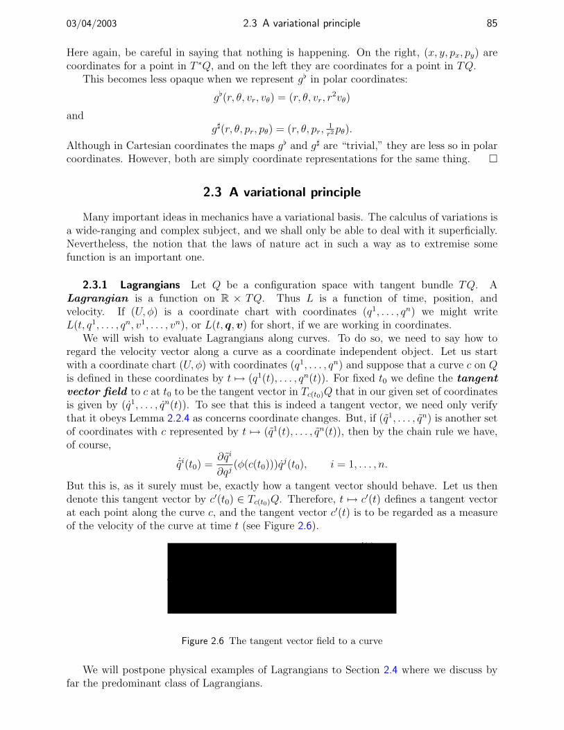
03/04/2003 2.3 A variational principle 85
Here again, be careful in saying that nothing is happening. On the right, (x, y, px, py) arecoordinates for a point in T ∗Q, and on the left they are coordinates for a point in TQ.
This becomes less opaque when we represent g[ in polar coordinates:
g[(r, θ, vr, vθ) = (r, θ, vr, r2vθ)
andg](r, θ, pr, pθ) = (r, θ, pr,
1r2pθ).
Although in Cartesian coordinates the maps g[ and g] are “trivial,” they are less so in polarcoordinates. However, both are simply coordinate representations for the same thing.
2.3 A variational principle
Many important ideas in mechanics have a variational basis. The calculus of variations isa wide-ranging and complex subject, and we shall only be able to deal with it superficially.Nevertheless, the notion that the laws of nature act in such a way as to extremise somefunction is an important one.
2.3.1 Lagrangians Let Q be a configuration space with tangent bundle TQ. ALagrangian is a function on R × TQ. Thus L is a function of time, position, andvelocity. If (U, φ) is a coordinate chart with coordinates (q1, . . . , qn) we might writeL(t, q1, . . . , qn, v1, . . . , vn), or L(t, q,v) for short, if we are working in coordinates.
We will wish to evaluate Lagrangians along curves. To do so, we need to say how toregard the velocity vector along a curve as a coordinate independent object. Let us startwith a coordinate chart (U, φ) with coordinates (q1, . . . , qn) and suppose that a curve c on Qis defined in these coordinates by t 7→ (q1(t), . . . , qn(t)). For fixed t0 we define the tangentvector field to c at t0 to be the tangent vector in Tc(t0)Q that in our given set of coordinatesis given by (q1, . . . , qn(t)). To see that this is indeed a tangent vector, we need only verifythat it obeys Lemma 2.2.4 as concerns coordinate changes. But, if (q1, . . . , qn) is another setof coordinates with c represented by t 7→ (q1(t), . . . , qn(t)), then by the chain rule we have,of course,
˙qi(t0) =∂qi
∂qj(φ(c(t0)))q
j(t0), i = 1, . . . , n.
But this is, as it surely must be, exactly how a tangent vector should behave. Let us thendenote this tangent vector by c′(t0) ∈ Tc(t0)Q. Therefore, t 7→ c′(t) defines a tangent vectorat each point along the curve c, and the tangent vector c′(t) is to be regarded as a measureof the velocity of the curve at time t (see Figure 2.6).
c(t)
c′(t)
Figure 2.6 The tangent vector field to a curve
We will postpone physical examples of Lagrangians to Section 2.4 where we discuss byfar the predominant class of Lagrangians.
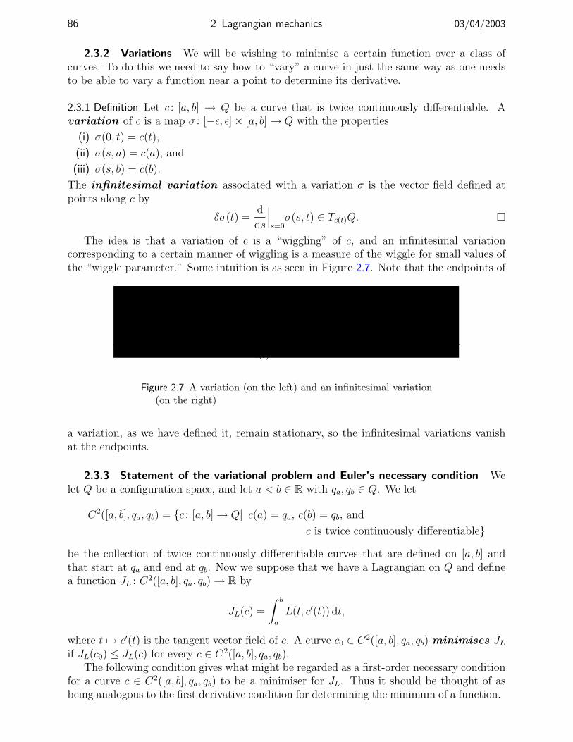
86 2 Lagrangian mechanics 03/04/2003
2.3.2 Variations We will be wishing to minimise a certain function over a class ofcurves. To do this we need to say how to “vary” a curve in just the same way as one needsto be able to vary a function near a point to determine its derivative.
2.3.1 Definition Let c : [a, b] → Q be a curve that is twice continuously differentiable. Avariation of c is a map σ : [−ε, ε]× [a, b] → Q with the properties
(i) σ(0, t) = c(t),
(ii) σ(s, a) = c(a), and
(iii) σ(s, b) = c(b).
The infinitesimal variation associated with a variation σ is the vector field defined atpoints along c by
δσ(t) =d
ds
∣∣∣s=0
σ(s, t) ∈ Tc(t)Q.
The idea is that a variation of c is a “wiggling” of c, and an infinitesimal variationcorresponding to a certain manner of wiggling is a measure of the wiggle for small values ofthe “wiggle parameter.” Some intuition is as seen in Figure 2.7. Note that the endpoints of
c(t)
σ(s, t)
c(t)
δσ(t)
Figure 2.7 A variation (on the left) and an infinitesimal variation(on the right)
a variation, as we have defined it, remain stationary, so the infinitesimal variations vanishat the endpoints.
2.3.3 Statement of the variational problem and Euler’s necessary condition Welet Q be a configuration space, and let a < b ∈ R with qa, qb ∈ Q. We let
C2([a, b], qa, qb) = c : [a, b] → Q| c(a) = qa, c(b) = qb, and
c is twice continuously differentiable
be the collection of twice continuously differentiable curves that are defined on [a, b] andthat start at qa and end at qb. Now we suppose that we have a Lagrangian on Q and definea function JL : C2([a, b], qa, qb) → R by
JL(c) =
∫ b
a
L(t, c′(t)) dt,
where t 7→ c′(t) is the tangent vector field of c. A curve c0 ∈ C2([a, b], qa, qb) minimises JL
if JL(c0) ≤ JL(c) for every c ∈ C2([a, b], qa, qb).The following condition gives what might be regarded as a first-order necessary condition
for a curve c ∈ C2([a, b], qa, qb) to be a minimiser for JL. Thus it should be thought of asbeing analogous to the first derivative condition for determining the minimum of a function.

03/04/2003 2.3 A variational principle 87
2.3.2 Theorem If a curve c ∈ C2([a, b], qa, qb) minimises JL then for any chart (U, φ) withthe property that the image of c intersects U, the representation t 7→ q(t) of c in that chartmust satisfy
d
dt
( ∂L
∂vi
)− ∂L
∂qi= 0, i = 1, . . . , n,
at (t,q(t), q(t)) for each t with the property that c(t) ∈ U.
Proof Let us first show that if c is a minimiser, then any subarc of c is also a minimiser.Thus let t1, t2 ∈ [a, b] satisfy a ≤ t1 < t2 ≤ b, and define a curve c : [t1, t2] → Q by c(t) = c(t)(i.e., c is the restriction of c to [t1, t2]). With t1 and t2 as defined we can also define theset of curves C2([t1, t2], c(t1), c(t2)) analogously to our definition of C2([a, b], qa, qb). We alsodefine a function JL on the set of curves C2([t1, t2], c(t1), c(t2)) by
JL(c) =
∫ t2
t1
L(t, c′(t)) dt.
We claim that if c is a minimiser for JL, then c is a minimiser for JL. Indeed, if c were not aminimiser for JL, this could imply the existence of a curve c1 ∈ C2([t1, t2], c(t1), c(t2)) withthe property that JL(c1) < JL(c). Now define a curve c1 : [a, b] → Q by
c1(t) =
c(t), t ∈ [a, t1]
c1(t), t ∈ [t1, t2]
c(t), ∈ [t2, b].
We then have
JL(c1) =
∫ t1
a
L(t, c′(t)) dt+
∫ t2
t1
L(t, c′1(t)) dt+
∫ b
t2
L(t, c′(t)) dt
<
∫ t1
a
L(t, c′(t)) dt+
∫ t2
t1
L(t, c′(t)) dt+
∫ b
t2
L(t, c′(t)) dt
=
∫ b
a
L(t, c′(t)) dt = JL(c).
This would complete our assertion that the restriction of c to any subinterval of [a, b] is itselfa minimiser, but for the fact that the curve c1 may not be twice continuously differentiable, asit may fail to be differentiable at t1 and t2. However, one may show (see Exercise E2.18) thatit is possible to modify c1 slightly to a curve c1 so that c1 is twice continuously differentiableon [a, b], and so that |JL(c1)− JL(c1)| ≤ ε for any ε > 0. In this way, one can ensure thatJL(c1) < JL(c), contradicting the fact that c is a minimiser.
The above argument says that c is a minimiser along every subinterval of [a, b] if it is aminimiser along the entire interval. Therefore, if (U, φ) is a chart so that c(t) ∈ U for somet ∈ [a, b], if c is a minimiser on [a, b], it is also a minimiser for the curve restricted to aninterval [t1, t2] with the property that c(t) ∈ U for t ∈ [t1, t2]. The upshot is that withoutloss of generality, we may suppose that the curve c lies in the domain of a chart (U, φ), andwe do this for the remainder of the proof.
Let σ be a variation of c and let cσ,s ∈ C2([a, b], qa, qb) be defined by cσ,s(t) = σ(s, t).Consider the function fσ defined on [−ε, ε] by fσ(s) = JL(cσ,s). If c is a minimiser for JL then

88 2 Lagrangian mechanics 03/04/2003
s = 0 should be a minimum of fσ for every variation σ of c. We let qσ,s be the coordinaterepresentative of cσ,s. We have
0 =d
ds
∣∣∣s=0
fσ(s) =d
ds
∣∣∣s=0
∫ b
a
L(t, qσ,s(t), qσ,s(t)) dt
=
∫ b
a
(∂L
∂qi
dqiσ,s(t)
ds
∣∣∣s=0
+∂L
∂vi
dqiσ,s(t)
ds
∣∣∣s=0
)dt.
Now note thatdqi
σ,s(t)
ds
∣∣∣s=0
=d
ds
∣∣∣s=0
dqiσ,s
dt=
d
dt
dqiσ,s(t)
ds
∣∣∣s=0
.
Therefore
0 =d
ds
∣∣∣s=0
fσ(s) =
∫ b
a
(∂L
∂qi
dqiσ,s(t)
ds
∣∣∣s=0
+∂L
∂vi
d
dt
dqiσ,s(t)
ds
∣∣∣s=0
)dt
=
∫ b
a
(∂L
∂qi
dqiσ,s(t)
ds
∣∣∣s=0
− d
dt
( ∂L∂vi
))dqiσ,s(t)
ds
∣∣∣s=0
dt+∂L
∂vi
dqiσ,s(t)
ds
∣∣∣s=0
∣∣∣∣t=b
t=b
=
∫ b
a
(∂L
∂qi
dqiσ,s(t)
ds
∣∣∣s=0
− d
dt
( ∂L∂vi
))dqiσ,s(t)
ds
∣∣∣s=0
dt
where in the next to last step we have used integration by parts, and in the last step wehave used the fact that an infinitesimal variation vanishes at the endpoints. Since∫ b
a
(∂L
∂qi
dqiσ,s(t)
ds
∣∣∣s=0
− d
dt
( ∂L∂vi
))dqiσ,s(t)
ds
∣∣∣s=0
dt = 0
for every variation, this means thatdqi
σ,s(t)
ds
∣∣∣s=0
can be arbitrary, and so the only way for the
integral to vanish is for∂L
∂qi− d
dt
( ∂L∂vi
)to be zero when evaluated at (q, q(t), q(t)).
The equationsd
dt
( ∂L∂vi
)− ∂L
∂qi= 0, i = 1, . . . , n,
are called the Euler-Lagrange equations , and they are what we will be primarily con-cerned with in the remainder of these notes. Though innocent enough in appearance, theyhide an enormous amount of beautiful structure. Note that the Euler-Lagrange equations areonly necessary conditions. A solution to the Euler-Lagrange equations may or may not be anactual minimiser. The common language is to call a curve in C2(qa, qb, [a, b]) an extremalwhen it satisfies the Euler-Lagrange equations. This reflects the fact that the Euler-Lagrangeequations are essentially analogous to the first derivative conditions in calculus.
Let’s look at a very simple example.
2.3.3 Example (Example 2.1.5 cont’d) We work again with Q = R2 and its two coordinatecharts (U1, φ1) and (U2, φ2). We define a Lagrangian on Q by defining it in the coordinatechart (U1, φ1) to be
L(t, x, y, vx, vy) =1
2(v2
x + v2y).

03/04/2003 2.3 A variational principle 89
Suppose that we have a curve t 7→ (x(t), y(t)) that is a minimiser for JL for some interval andwith some endpoints. Then the Euler-Lagrange equations say that this curve must satisfy
d
dt
( ∂L∂vx
)− ∂L
∂x=
d
dtvx = vx(t) = x(t) = 0
d
dt
( ∂L∂vy
)− ∂L
∂y=
d
dtvy = vy(t) = y(t) = 0.
Thus the Euler-Lagrange equations are the simple second-order differential equations
x(t) = 0, y(t) = 0,
and these have solution x(t) = x(0) + x(0)t and y(t) = y(0) + y(0)t. These describe straightlines in the plane Q = R2.
Now let us look at the same example in the polar coordinate chart (U2, φ2). First weneed to determine the Lagrangian in these coordinates. Using the transformation rule (2.5)we have
vx =∂x
∂rvr +
∂x
∂θvθ = cos θvr − r sin θvθ
vy =∂y
∂rvr +
∂y
∂θvθ = sin θvr + r cos θvθ.
With these relations we readily compute
v2x + v2
y = v2r + r2v2
θ
so that
L =1
2(v2
r + r2v2θ).
The Euler-Lagrange equations are then
d
dt
( ∂L∂vr
)−∂L∂r
=d
dtvr − r(t)v2
θ(t) = vr(t)− r(t)v2θ(t) = r(t)− r(t)θ2(t) = 0
d
dt
( ∂L∂vθ
)− ∂L
∂θ=
d
dt(r2vθ) = r2vθ(t) + 2r(t)r(t)vθ(t) = r2(t)θ(t) + 2r(t)r(t)θ(t) = 0.
That is, the Euler-Lagrange equations are the two coupled second-order differential equations
r(t)− r(t)θ2(t) = 0, r2(t)θ(t) + 2r(t)r(t)θ(t) = 0.
These equations are less amenable to solution by inspection than their Cartesian coordinatecounterparts. However, since we know the Cartesian solutions and the change of coordinateformulae, we may in principal write the solutions to the polar coordinate equations. However,to do so is straightforward, and not a very interesting display of symbology.
2.3.4 The Euler-Lagrange equations and changes of coordinate In the previousexample, we wrote the Euler-Lagrange equations in two different sets of coordinates, andsomehow we think that the two sets of equations should represent the same thing. Let usexplore exactly what is meant by this. First of all, we remark that the problem of minimisingJL over curves in C2([a, b], qa, qb) obviously does not depend upon any choice of coordinates.Now, if the problem statement is not dependent on coordinate chart, then so should be anystatements relating to its solution. Thus we should hope that the Euler-Lagrange equationsare in some sense coordinate invariant. Indeed they are, and in just the way of the followingresult.

90 2 Lagrangian mechanics 03/04/2003
2.3.4 Proposition Let Q be a configuration space with (q1, . . . , qn) and (q1, . . . , qn) coordi-nates for Q. If L is a Lagrangian on Q then
d
dt
( ∂L
∂vi
)− ∂L
∂qi=∂qj
∂qi
[d
dt
( ∂L
∂qj
)− ∂L
∂qj
].
In particular, the Euler-Lagrange equations are satisfied in the coordinates (q1, . . . , qn) if andonly if they are satisfied in the coordinates (q1, . . . , qn).
Proof Note that by (2.5) we have
∂vj
∂vi=∂qj
∂qi,
∂vj
∂qi=
∂2qj
∂qi∂qkvk
Therefore, using the chain rule, we have
∂L
∂vi=∂L
∂vj
∂vj
∂vi+∂L
∂qj
∂qj
∂vi
=∂L
∂vj
∂qj
∂qi
∂L
∂qi=∂L
∂vj
∂vj
∂qi+∂L
∂qj
∂qj
∂qi
=∂L
∂vj
∂2qj
∂qi∂qkvk +
∂L
∂qj
∂qj
∂qi.
Now note thatd
dt
( ∂L∂vi
)=
d
dt
( ∂L∂vj
)∂qj
∂qi+∂L
∂vj
∂2qj
∂qi∂qk˙qk.
Therefore, simple addition verifies the first part of the proposition. As for the second as-sertion, it follows from the first since the matrix with components ∂qj
∂qi , i, j = 1, . . . , n, isinvertible.
2.3.5 Important remark Note that the components of the Euler-Lagrange equations transformjust like the components of a one-form on Q. However, the Euler-Lagrange equations are nota one-form, because their coefficients depend time, velocity, and acceleration. A utilisationof this fact is to be found in [Lewis 2000c].
Let’s see how this plays out in our running example.
2.3.6 Example (Example 2.1.5 cont’d) We have, as usual, Q = R2 with its Cartesian andpolar coordinate charts. In Example 2.3.3 we derived the Euler-Lagrange equations for aparticular Lagrangian in both sets of coordinates. Let us verify that these equations areindeed related as in Proposition 2.3.4.
In Cartesian coordinates the Euler Lagrange equations were
x = 0, y = 0,
and in polar coordinates we had
r − rθ2 = 0, r2θ + 2rrθ = 0.
03/04/2003 2.4 Simple mechanical systems 91
We compute
∂x
∂r
[d
dt
( ∂L∂vx
)−∂L∂x
]+∂y
∂r
[d
dt
( ∂L∂vy
)−∂L∂y
]= cos θ(x) + sin θ(y)
= cos θ(cos θr − 2 sin θrθ − r cos θθ2 − r sin θθ)+
sin θ(sin θr + 2 cos θrθ − r sin θθ2 + r cos θθ)
= r − rθ2.
Similarly we compute
∂x
∂θ
[d
dt
( ∂L∂vx
)−∂L∂x
]+∂y
∂θ
[d
dt
( ∂L∂vy
)−∂L∂y
]= −r sin θ(x) + r cos θ(y)
= − r sin θ(cos θr − 2 sin θrθ − r cos θθ2 − r sin θθ)+
r cos θ(sin θr + 2 cos θrθ − r sin θθ2 + r cos θθ)
= r2θ + 2rrθ.
Thus the components do indeed transform as they ought to, although a direct verificationof this, even in a simple example, is a not entirely pleasant task.
2.4 Simple mechanical systems
“Simple” mechanical systems are not so named because they behave in a particularlysimple manner. The usage of the word simple here has a precise meaning, and the fact ofthe matter is that the vast majority of mechanical systems one encounters are “simple” byour usage of the word. Simple mechanical systems are characterised by having a special sortof Lagrangian.
2.4.1 Kinetic energy The most important feature of a simple mechanical system isthat it has kinetic energy. This means something very particular in the terminology weintroduced in Section 2.2.4. Let g be a Riemannian metric on Q. The kinetic energyassociated with g is the function K on TQ defined by K(vq) = 1
2g(vq, vq). Note that we
need a Riemannian metric to define kinetic energy! This is why we introduced the conceptof a Riemannian metric. However, when working with an example, one can often readilydetermine by elementary methods its kinetic energy in a set of coordinates (q1, . . . , qn),without knowing what is the Riemannian metric in these coordinates. But the fact of thematter is that the Riemannian metric is there. To recover it proceed as follows. Thekinetic energy you derive will be a function K(q1, . . . , qn, v1, . . . , vn). The components gij,i, j = 1, . . . , n, of the corresponding Riemannian metric are then determined by
gij =∂2K
∂vi∂vj, i, j = 1, . . . , n.
Note that if you apply this formula and the components for g turn out to involve thevelocities, then you have either made a mistake, or the system you are dealing with is not asimple mechanical system.
Let us see how this works in our simple example.

92 2 Lagrangian mechanics 03/04/2003
2.4.1 Example (Example 2.1.5 cont’d) We now add some physics to this example. The con-figuration space Q = R2 we take to be the configuration space for a particle of mass mmoving in a plane. Thus we have chosen an appropriate coordinate system for a Galileanspacetime to reduce ourselves to this situation. In Cartesian coordinates, the kinetic energyof such a mass is simply
K =1
2m(x2 + y2) =
1
2m(v2
x + v2y).
One then computes
gij =∂2K
∂vi∂vj= mδij, i, j = 1, . . . , n.
Therefore, the kinetic energy of a particle in the plane is in exact correspondence with thestandard Riemannian metric on R2, scaled by m > 0.
Although we have illustrated this correspondence via the Cartesian coordinate system,it does not rely on this system of coordinates. Let us see how this pans out in polarcoordinates. Clearly the particle example is essentially like the Example 2.2.18 as concernsthe Riemannian metric, and like Example 2.3.3 as concerns the Lagrangian. Referring tothose examples, the Riemannian metric g in polar coordinates is
g = m(dr ⊗ dr + r2dθ ⊗ dθ
),
and we also have K = 12m(v2
r + r2v2θ) so that
∂2K
∂vi∂vj=
m, i = 1,
mr2, i = 2,
0, otherwise.
This demonstrates that ∂2K∂vi∂vj = gij, even in polar coordinates.
2.4.2 Remarks 1. Since we have a 1–1 correspondence between the concept of kinetic energyand a Riemannian metric, let us agree to use the latter as basic, since, as we shall see, aRiemannian metric possesses many interesting properties.
2. In very simple examples like the previous one, one can see that it is a bit overkill to for-mally compute ∂2K
∂vi∂vj in order to determine the components of the Riemannian metric;one can simply look at the expression for kinetic energy and write down the corre-sponding metric components. However, for more complicated system formed on multiplecomponents, one often will write the kinetic energy of each component, then taking thetotal kinetic energy to be the sum of the component energies. In this case, the formulagij = ∂2K
∂vi∂vj can be used, perhaps in a symbolic manipulation language, to produce themetric components with relative ease.
2.4.2 Potential energy The notion of potential energy is quite simple as concerns itsbasic definition: a potential function is a function V on the configuration space Q. Inparticular, it is a function independent of velocity.
2.4.3 Example (Example 2.1.5 cont’d) Let us resume talking about a mass m moving aboutin the plane. Now let us suppose that the plane is oriented in such a way that the forceof gravity acts in the y-direction in Cartesian coordinates. In this case, our elementary

03/04/2003 2.4 Simple mechanical systems 93
physics tells us that potential energy should be a “storage function” for the energy thatthe system has when it is at a given height. This, of course, requires us to declare someheight as being the zero height, where the body has no gravitational potential energy. Thischoice is arbitrary, so let us choose it to be y0. The gravitational potential energy is thenV = mag(y − y0) where ag is the acceleration due to gravity (e.g., ag ≈ 13.24m/sec2 on thesurface of Neptune). One of the drawbacks of the classical (due to Einstein, I expect) use ofg for a Riemannian metric is that one cannot now use that symbol for the acceleration dueto gravity.
Let us see what this function looks like in polar coordinates. Define r0 ∈ R+ andθ0 ∈ (−π, π) by y0 = r0 sin θ0. This supposes that y0 6= 0. We then have
y − y0 = r sin θ − r0 sin θ0,
so the gravitational potential in polar coordinates is
V = mag(r sin θ − r0 sin θ0).
Note that, even in the Newtonian world, this is really only an approximation of thegravitational force (see Exercise E2.24).
Although the concept of potential energy is benign enough, there is actually a reasonwhy it is a wee bit subtle, and we will touch on that soon.
2.4.3 The Euler-Lagrange equations for simple mechanical systems We now havethe data to say what we mean by a simple mechanical system.
2.4.4 Definition A simple mechanical system is a triple (Q, g, V ) where
(i) Q is a configuration space,
(ii) g is a Riemannian metric on Q, and
(iii) V is a potential energy function on Q.
The Lagrangian associated to a simple mechanical system (Q, g, V ) is the function on TQdefined by
L(vq) =1
2g(vq, vq)− V (q).
One might well ask, “Why use a minus sign on the potential?” Indeed, the “natural”quantity seems to be the total energy 1
2g(vq, vq) + V (q). The reasons for using the minus
sign cannot be explicated in a coherent manner until we look at the Lagrange-d’Alembertprinciple in Section 2.5. For now, let us just say that we use it because it works.
Let us look at the Euler-Lagrange equations for simple mechanical systems. To do so,given a potential function V on Q, define a vector field gradV on Q by
gradV (q) = g](dV (q)).
Note that since dV is a one-form, gradV is indeed a vector field as claimed. In coordinateswe have
gradV = gij ∂V
∂qj
∂
∂qi.
Now we may state the following result.

94 2 Lagrangian mechanics 03/04/2003
2.4.5 Proposition Let (Q, g,V) be a simple mechanical system with associated Lagrangian L.Let c : I → Q be a curve which is represented by t 7→ (q1(t), . . . , qn(t)) in a coordinate chart(U, φ). The following statements are equivalent:
(i) t 7→ (q1(t), . . . , qn(t)) satisfies the Euler-Lagrange equations for the Lagrangian L;
(ii) t 7→ (q1(t), . . . , qn(t)) satisfies the second-order differential equation
qi + Γijkq
jqk = −(grad V)i, i = 1, . . . , n,
where Γijk, i, j, k = 1, . . . , n, are functions of q defined by
Γijk =
1
2gi`(∂gj`
∂qk+∂gk`
∂qk− ∂gjk
∂q`
).
Proof In coordinates we have
L =1
2gjkv
jvk − V (q).
We therefore have∂L
∂v`= g`jv
j,∂L
∂q`=
1
2
∂gjk
∂q`vjvk − ∂V
∂q`.
Therefore the Euler-Lagrange equations are
g`j qj +(∂g`j
∂qk− 1
2
∂gjk
∂q`
)qj qk +
∂V
∂q`= 0. (2.8)
Since the expression qj qk is symmetric with respect to transposing the indices j and k, onlythe symmetric part of the expression
A`jk ,∂g`j
∂qk− 1
2
∂gjk
∂q`
with respect to the indices j and k will contribute to the expression(∂g`j
∂qk− 1
2
∂gjk
∂q`
)qj qk.
But the symmetric part of A`jk with respect to j and k is
1
2(A`jk + A`kj) =
1
2
(∂gj`
∂qk+∂gk`
∂qj− ∂gjk
∂q`
).
The result now follows by multiplying (2.8) by gi`.
We shall see in the next section the meaning of the functions Γijk, i, j, k = 1, . . . , n. They
represent a very important object in the study of simple mechanical systems.Let us see how the description of the Euler-Lagrange equations plays out for our running
example.
2.4.6 Example (Example 2.1.5 cont’d) We take as our simple mechanical system (Q =R2, g, V ) where g is the Riemannian metric of Example 2.4.1 and V is the potential functionof Example 2.4.3.

03/04/2003 2.4 Simple mechanical systems 95
In Cartesian coordinates, the resulting Lagrangian on TQ is given by
L(x, y, vx, vy) =1
2m(v2
x + v2y)−mag(y − y0).
The Euler-Lagrange equations are then readily computed to be
mx = 0, my +mag = 0. (2.9)
Given thatg = m(dx⊗ dx+ dy ⊗ dy)
in these coordinates, one readily determines that the functions Γijk are zero for all i, j, k = 1, 2.
One also sees that
gradV = ag∂
∂y.
Therefore the equations of part (ii) of Proposition 2.4.5 read
x = 0, y = −ag,
and these equations are obviously equivalent to the equations (2.9).Now let us also check that things work out in polar coordinates. In these coordinates we
have
L(r, θ, vr, vθ) =1
2m(v2
r + r2v2θ)−mag(r sin θ − r0 sin θ0).
The Euler-Lagrange equations are then
mr −mrθ2 +mag sin θ = 0, mr2θ + 2mrrθ +magr cos θ = 0. (2.10)
To check the equations of part (ii) of Proposition 2.4.5, we note that
g = m(dr ⊗ dr + r2dθ ⊗ dθ),
and a simple, slightly tedious, computation gives
Γrθθ = −r, Γθ
rθ = Γθθr =
1
r,
with the remaining Γ’s being zero. One also computes
gradV = ag sin θ∂
∂r+
1
rag cos θ
∂
∂θ.
Therefore the equations of part (ii) of Proposition 2.4.5 are
r − rθ2 = −ag sin θ, θ +2
rrθ = −1
rag cos θ.
These equations are clearly equivalent to the equations (2.10).Note that the equations are independent of the datum y0 from which potential energy
was measured.

96 2 Lagrangian mechanics 03/04/2003
2.4.4 Affine connections In the previous section, we saw arise the functions Γijk,
i, j, k = 1, . . . , n, defined in a set of coordinates for a configuration space Q. We shall nowaddress the question, “What are these functions?” The answer may seem weird, but it isnonetheless the answer, dictated by the physics of the problem.
In order to make the definition, we need a few simple concepts. If X is a vector field onQ and f is a function on Q, then fX is also a vector field on Q with (fX)(q) = f(q)X(q)for each q ∈ Q. Thus fX is simply the vector field with the vectors scaled by the values off . Also, given a vector field X and a function f we define the Lie derivative of f withrespect to X to be the function on Q defined by
L Xf(q) = 〈df(q);X(q)〉 .
In coordinates (q1, . . . , qn) we have
L Xf = X i ∂f
∂qi,
thus L Xf may be known to you as the “directional derivative.”With this language, we make the following definition.
2.4.7 Definition An affine connection on a configuration space Q is an assignment to eachpair of vector fields X and Y on Q a vector field ∇XY and the assignment has the properties:
(i) the map (X, Y ) 7→ ∇XY is bilinear with respect to multiplication by real numbers;
(ii) for each pair of vector fields X and Y and for each function f on Q, we have ∇fXY =f(∇XY );
(iii) for each pair of vector fields X and Y and for each function f on Q, we have ∇X(fY ) =f(∇XY ) + (L Xf)Y .
We also call ∇XY the covariant derivative of Y with respect to X.
What can this possibly have to do with mechanics?! Well, let us see what an affineconnection looks like in coordinates. Let (U, φ) be a coordinate chart with coordinates(q1, . . . , qn). Given a pair of coordinate vector fields ∂
∂qi and ∂∂qj their covariant derivative
is also a vector field. Therefore, ∇ ∂
∂qi
∂∂qj must be a linear combination of the basis vector
fields ∂∂q1 , . . . ,
∂∂qn. Thus there exists n functions Γk
ij, k = 1, . . . , n, so that
∇ ∂
∂qi
∂
∂qj= Γk
ij
∂
∂qk. (2.11)
As this must be true for each i, j = 1, . . . , n, this defines n3 functions Γkij, i, j, k = 1, . . . , n,
of the coordinates (q1, . . . , qn) which are called the Christoffel symbols for the affineconnection ∇ in the coordinate chart (U, φ). Note that the affine connection is determineduniquely in a coordinate chart by its Christoffel symbols. This is made clear by the followingresult.
2.4.8 Proposition Let ∇ be an affine connection on a configuration space Q and let X andY be vector fields on Q. If (U, φ) is a coordinate chart with coordinates (q1, . . . , qn) thenwe have
∇XY =(∂Yk
∂qiXi + Γk
ijXiYj) ∂
∂qk
on U, where Γkij, i, j, k = 1, . . . , n, are the Christoffel symbols for ∇ in the coordinate chart
(U, φ).

03/04/2003 2.4 Simple mechanical systems 97
Proof This follows by the properties of an affine connection. Indeed we have
∇XY = ∇Xi ∂
∂qiY j ∂
∂qj
= X iY j∇ ∂
∂qi
∂
∂qj+X iL ∂
∂qiY j ∂
∂qj
=(X iY jΓk
ij +X i∂Yk
∂qi
) ∂
∂qk,
just as claimed.
Now we see that Γ’s may come up as claimed, but it is still not clear how the Γ’s ofProposition 2.4.5 are related to the Christoffel symbols. To see how this relationship isestablished, we will associate with a Riemannian metric, i.e., with kinetic energy, a uniqueaffine connection. In order to carry this out, we need to have at hand the concept of a Liebracket between two vector fields X and Y on Q. This is defined to be the vector field[X,Y ] on Q which, in any set of coordinates (q1, . . . , qn) is given by
[X, Y ] =(∂Y i
∂qjXj − ∂X i
∂qjY j) ∂
∂qi. (2.12)
Of course, for this definition to make sense, one must check that this definition does notdepend on coordinates, and we leave this straightforward calculation to the reader (Exer-cise E2.15). The Lie bracket is an extremely important object in differential geometry, and wewill put it to rather pedestrian usage here in our discussion of affine connections. However,in Sections 2.6 and 4.5, we shall see a more interesting application of the Lie bracket.
Let us proceed with our discussion. The following result is not difficult to prove, butits proof is perhaps a bit sophisticated for our purposes here. We refer the reader to, forexample, [Kobayashi and Nomizu 1963] for a proof.
2.4.9 Theorem Let g be a Riemannian metric on a configuration space Q. There exists a
unique affine connectiong
∇ on Q with the following properties:
(i)g
∇XY −g
∇YX = [X,Y] for all vector fields X and Y on Q;
(ii) L Z(g(X,Y)) = g(g
∇ZX,Y) + g(X,g
∇ZY) for all vector fields X, Y, and Z on Q.
Furthermore, in a set of coordinates (q1, . . . , qn) for Q, the Christoffel symbols forg
∇ aregiven by
g
Γijk =
1
2gi`(∂gj`
∂qk+∂gk`
∂qk− ∂gjk
∂q`
).
The affine connectiong
∇ is the Levi-Civita connection corresponding to the Riemannianmetric g.
Now we at last see the meaning of the functions Γijk in the statement of Proposition 2.4.5.
They are the Christoffel symbols of an affine connection, called the Levi-Civita connection,which one may associate with the Riemannian metric defining the kinetic energy. Let us looka little more closely at the differential equation of part (ii) of Proposition 2.4.5, concentratingon the case when the case when the potential energy function is zero. The differentialequation in question is then,
qi +g
Γijkq
j qk = 0, i = 1, . . . , n,

98 2 Lagrangian mechanics 03/04/2003
where we now acknowledge explicitly the dependence of the Γ’s on g. Clearly, there isnothing preventing us from talking about this equation when we do not use the Christoffelsymbols for the Levi-Civita connection, but rather Christoffel symbols for a general affineconnection. To this end, let ∇ be a general affine connection on Q. A curve c : I → Q iscalled a geodesic for ∇ when for any t0 ∈ I and any coordinate chart (U, φ) around c(t0)with coordinates (q1, . . . , qn), the coordinate representation t 7→ (q1(t), . . . , qn(t)) satisfiesthe differential equation
qi + Γijkq
j qk = 0, i = 1, . . . , n,
where Γijk, i, j, k = 1, . . . , n, are the Christoffel symbols of ∇ in the coordinate chart (U, φ).
Of course, for this to make sense, the definition needs to be shown to be independent of coor-dinates. We leave this only slightly tedious computation to the reader (Exercise E2.26). Note,however, that each of the terms in the geodesic equations are not coordinate independent!Thus one should not write qi as a tangent vector, since it does not obey a transformation lawlike a tangent vector should! To talk about acceleration as a vector one genuinely needs anaffine connection. In this case, the notation one uses for the quantity which in coordinatesis qi + Γi
jkqj qk is ∇c′(t)c
′(t), and a geodesic is a curve c for which ∇c′(t)c′(t) = 0.
We may now offer the following coordinate independent restatement of Proposition 2.4.5.
2.4.10 Theorem Let (Q, g,V) be a simple mechanical system with associated Lagrangian L.Let c ∈ C2([a, b], qa, qb). The following statements are equivalent:
(i) c satisfies the Euler-Lagrange equations for the Lagrangian L;
(ii) c satisfiesg
∇c′(t)c′(t) = − grad V(c(t)).
Let us see how this looks in our running example.
2.4.11 Example (Example 2.1.5 cont’d) The Q = R2 example we have been using, althoughsimple, is ample to illustrate why one cannot regard acceleration as a tangent vector. On Qwe consider a curve c : R → Q defined in Cartesian coordinates by
c(t) = (cos t, sin t).
Thus c describes a circle. In Cartesian coordinates we then have (x(t), y(t)) = (cos t, sin t)so that
(x(t), y(t)) = (− sin t, cos t), (x(t), y(t)) = (− cos t,− sin t).
In polar coordinates the curve is represented by (r(t), θ(t)) = (1, t), but note that r(t) andθ(t) are only defined for t ∈ (−π, π). We readily compute
(r(t), θ(t)) = (0, 1), (r(t), θ(t)) = (0, 0).
Therefore the acceleration along the curve is zero in polar coordinates, but nonzero in polarcoordinates. This precludes acceleration from being a tangent vector since it cannot be bothzero and nonzero.
Now let us look at the acceleration represented by the Levi-Civita connection corre-sponding to the Riemannian metric g from Example 2.4.1. In Cartesian coordinates, theChristoffel symbols are zero so we have
g
∇c′(t)c′(t) = x
∂
∂x+ y
∂
∂y= − cos t
∂
∂x− sin t
∂
∂y.

03/04/2003 2.5 Forces in Lagrangian mechanics 99
In polar coordinates, the Christoffel symbols were computed in Example 2.4.1, and usingthese we have
g
∇c′(t)c′(t) = (r − rθ2)
∂
∂r+(θ + 2
rrθ) ∂∂θ
= − ∂
∂r.
Thus in both Cartesian and polar coordinates, the quantityg
∇c′(t)c′(t) is a vector of “unit
length” (if m = 1, remove the quotes) pointing towards the origin (see Figure 2.8). The
c′(t)
∇c′(t)c′(t)
c(t)
Figure 2.8 Velocity and “geometric acceleration” along a curve
quantityg
∇c′(t)c′(t) is sometimes called the geometric acceleration . Note that since the
geometric acceleration is nonzero, the curve c is not a geodesic. Well, of course it is not:geodesics, as we have seen, are straight lines for this affine connection.
2.4.12 Remark One often sees the Euler-Lagrange equations for a simple mechanical La-grangian L(vq) = 1
2g(vq, vq)− V (q) written as
M(q)q + C(q, q) +K(q) = 0,
or something similar to this, where M(q) is a matrix whose entries are gij(q) in some set ofcoordinates. In our manner of writing the equations of motion, the term C(q, q) is given by
gi`
g
Γ`jkq
j qk, and is called by some authors “Coriolis forces.” This, as we can see, is nonsensicalin a certain sense. The term C(q, q) makes no sense by itself. Indeed, as Example 2.4.11shows, this term in the equations can be zero in one set of coordinates, and nonzero inanother set of coordinates. The term C(q, q) should not be taken by itself as meaningful.
2.5 Forces in Lagrangian mechanics
If one wishes to talk about control theory for mechanical systems, as we do, then thenatural “inputs” for these systems are forces. In this section we discuss forces generally,concentrating on the various nature of forces which can arise in mechanical systems. Webegin with a discussion of how forces appear in the Euler-Lagrange equations.
2.5.1 The Lagrange-d’Alembert principle The appearance of forces in Newtonianmechanics is done using the laws Newton laid out as motivation. How one should go about

100 2 Lagrangian mechanics 03/04/2003
adding forces to the Euler-Lagrange equations is not altogether obvious. First let us say thata force on a configuration space Q is a map F : R×TQ→ T ∗Q which has the property thatF (t, vq) ∈ T ∗q Q. Thus a force is a function of time, position, and velocity, and for each fixedvalue (t, vq) of these arguments, it is a covector in the cotangent space T ∗q Q. Just why a forceshould naturally be regarded as a covector rather than a tangent vector is a question bestanswered by saying, “Because that’s the way it works out.” Some motivation may be drawnfrom Proposition 2.3.4 which indicates how that the Euler-Lagrange equations themselveschange like the components of a one-form under coordinate changes. In any event, we canwrite a force in coordinates as
F (t, q,v) = Fi(t, q,v)dqi,
for some function F1, . . . , Fn of time, configuration, and velocity, called the components
of the force F .The Lagrange-d’Alembert principle, often simply called “d’Alembert’s principle,” tells
us how a force F should appear in the Euler-Lagrange equations.
2.5.1 Definition Let L be a Lagrangian on a configuration space Q and let F be a force. Acurve c : [a, b] → Q satisfies the Lagrange-d’Alembert principle for the force F if forevery variation σ : [−ε, ε]× [a, b] → Q we have
d
ds
∣∣∣s=0
∫ b
a
L(t, d
dtσ(s, t)
)dt+
∫ b
a
〈F (t, c′(t)); δσ(t)〉 dt = 0.
The idea behind this definition is that when the external forces are not present, they makeno contribution in the second term in Definition 2.5.1. However, when they are present, theydo work, and this is evidently properly accounted for in the variational formulation whichwe call the Lagrange-d’Alembert principle.
Let us see what are the implications of the Lagrange-d’Alembert principle for the equa-tions describing the motion of a Lagrangian system in the presence of forces.
2.5.2 Proposition Let L be a Lagrangian on Q with F a force on Q. A curve c : [a, b] → Qsatisfies the Lagrange-d’Alembert principle if and only if for any coordinate chart (U, φ)which intersects the image of c, the coordinate representation t 7→ (q1(t), . . . , qn(t)) satisfies
d
dt
( ∂L
∂vi
)− ∂L
∂qi= Fi, i = 1, . . . , n, (2.13 )
where F1, . . . ,Fn are the components of F. The equations (2.13) are the forced Euler-Lagrange equations.
Proof Fix a coordinate chart (U, φ) which intersects the image of c. By considering vari-ations of c whose infinitesimal variation vanishes outside a coordinate chart, we may sup-pose that c(t) ∈ U for each t. Let σ be a variation of c with cσ,s the curve defined bycσ,s(t) = σ(s, t). Denote the coordinate representation of cσ,s by qσ,s. Then, by following thecalculations of Theorem 2.3.2, we arrive at∫ b
a
(∂L
∂qi
dqiσ,s(t)
ds
∣∣∣s=0
− d
dt
( ∂L∂vi
)+ Fi
)dqi
σ,s(t)
ds
∣∣∣s=0
dt = 0.
Since this must hold for every variation, the result follows.

03/04/2003 2.5 Forces in Lagrangian mechanics 101
Thus the manner in which one adds forces to the Euler-Lagrange equations, governedby the Lagrange-d’Alembert principle, is very simple: one merely sticks the componentsof the force on the right-hand side of the Euler-Lagrange equations. The question of whythis is the right thing to do often results in a pointless metaphysical discussion. The realreason is, “Because it works,” meaning that the Lagrange-d’Alembert principle agrees withmeasurement to a tolerable degree. Mathematical descriptions of our physical world mustbe a slave to empirical data.
2.5.2 Potential forces A potential force is one resulting from potential energy. Moreusefully, given a potential function V on Q, its potential force is the force given byF (t, vq) = −dV (q). In particular, potential forces are independent of time and velocity.2
However, potential forces are more than simply independent of time and velocity. Theyhave a useful property with respect to the “work” done by a mechanical system. We needto define work. One normally takes as the definition of work “force times distance.” This isfine for defining work done on straight line paths in Euclidean space. However, our settingis more general than this in several ways. First, we are working with general configurationspaces. Second, on a general configuration space, there is no such thing as a straight linepath. Thus we are led to the following definition. On a configuration space Q, we define thework done by a force F along a curve c : I → Q to be the quantity
W (F, c) =
∫I
〈F (t, c′(t)); c′(t)〉 dt. (2.14)
One should be able to readily see that this properly generalises the classical notion of work(see Exercise E2.27).
Now with this notion of work, we have the following characterisation of a potential force.A curve c : [a, b] → Q is closed if c(a) = c(b).
2.5.3 Proposition Let F be a force on a configuration space Q. The following statements areequivalent:
(i) the work done by F on any closed curve is zero;
(ii) F is a potential force.
Proof The implication (ii) =⇒ (i) is readily made. Indeed, if F is a potential force, thenF (t, vq) = −dV (q) for some function V . We then have
W (F, c) =
∫ b
a
〈F (t, c′(t)); c′(t)〉 dt
= −∫ b
a
〈dV (c(t)); c′(t)〉 dt
= −∫ b
a
dV (c(t))
dtdt
= − (V (c(b))− V (c(a))) = 0,
for every closed curve c : [a, b] → Q.
2One can actually define potential forces to be time-dependent by allowing V to depend on time. Some-times it is interesting to do this, but we shall not do so.

102 2 Lagrangian mechanics 03/04/2003
The implication (i) =⇒ (ii) goes as follows. Suppose that F is a potential force and letq0 ∈ Q. For q ∈ Q define V (q) ∈ R by
V (q) = −∫ 1
0
〈F (c(t)); c′(t)〉 dt,
where c : [0, 1] → Q is any curve satisfying c(0) = q0 and c(1) = q. We will first show thatthe function V defined in this manner does not depend on the choice made for the curvec. Let c1, c2 : [0, 1] → Q be two curves satisfying c1(0) = c2(0) = q0 and c1(1) = c2(1) = q.Define a curve σ : [0, 1] → Q by
σ(t) =
c1(2t), t ∈ [0, 1
2]
c2(2− 2t), t ∈ [12, 1].
Note that σ(0) = σ(1) so that ∫ 1
0
〈F (σ(t));σ′(t)〉 dt = 0.
However, we also have∫ 1
0
〈F (σ(t));σ′(t)〉 dt =
∫ 12
0
〈F (σ(t));σ′(t)〉 dt+
∫ 1
12
〈F (σ(t));σ′(t)〉 dt
=
∫ 1
0
〈F (c1(t)); c′1(t)〉 dt+
∫ 0
1
〈F (c2(t)); c′2(t)〉 dt,
from which we conclude that∫ 1
0
〈F (c1(t)); c′1(t)〉 dt =
∫ 1
0
〈F (c2(t)); c′2(t)〉 dt.
Thus our definition of V is independent of curve, as desired.Finally, let us show that F = −dV , thus making F a potential force. Let (U, φ) be
a coordinate chart around q ∈ Q and suppose that φ(q) = 0. Let Bε(0) be the ball ofradius ε centred at the origin in Rn, and suppose that Bε(0) ⊂ φ(U). Let v ∈ Rn and letx1 = ε
‖v‖v be the point on Bε(0) which lies in the direction of v. Denote q1 = φ−1(x1). Let
c : [0, 1] → Q be a curve with the properties
1. c(0) = q0;
2. c(1−ε‖v‖ ) = q1;
3. φ c(t) = ‖v‖(1−t)‖v‖+ε−1
x1, t ∈ [1−ε‖v‖ , 1].
Now we define ψ : [1−ε‖v‖ , 1] → R by
ψ(t) =
∫ t
1−ε‖v‖
〈F (φ c(s)); v〉 ds,
where F is the representation of F is the coordinate chart (U, φ). Let Vφ : Bε(0) → R bedefined by Vφ(x) = V φ−1(x). Note that with ψ defined as we have done, we have
Vφ(tv) = ψ(1− t), t ∈ [0, ε‖v‖ ].

03/04/2003 2.5 Forces in Lagrangian mechanics 103
Therefore we have
〈dVφ(0); v〉 = − d
dt
∣∣∣∣t=1
ψ(t).
By the definition of ψ this gives
〈dVφ(0); v〉 = −〈F (0); v〉.
If vq ∈ TqQ is the tangent vector whose coordinate representation in the chart (U, φ) is v,then this means that
〈dV (q); vq〉 = −〈F (q); vq〉.
Since our above construction can be done for any v ∈ Rn this shows that F (q) = −dV (q),as desired.
Of course, we have already seen a potential function, but let us explicitly identify theforce associated with it.
2.5.4 Example (Example 2.1.5 cont’d) We consider the gravitational potential introduced inExample 2.4.3. In Cartesian coordinates we had V (x, y) = mag(y − y0), so the potentialforce is simply
F = −dV = −magdy.
In polar coordinates we had V = mag(r sin θ− r0 sin θ0), so that the potential force in thesecoordinates is
F = −dV = −mag(sin θdr + r cos θdθ).
Were one to derive from “first principles” the formula for the potential force, one would havesome work to do, but using the blind calculations, it is quite simple.
Rayleigh
dissipation
function2.5.3 Dissipative forces A force F on a configuration space Q is a dissipative forceif 〈F (t, vq); vq〉 ≤ 0 for every (t, vq) ∈ R×TQ. A dissipative force is strictly dissipative ifstrict inequality holds for each vq ∈ TQ. Dissipative forces “dissipate energy.” Although wehave talked about kinetic energy and potential energy, we have not really talked about thetotal energy of a Lagrangian system. Certainly, for a simple mechanical system (Q, g, V )one is inclined to define the total energy to be the sum of the kinetic and potential energy:E(vq) = 1
2g(vq, vq) + V (q). This can be generalised for arbitrary Lagrangians.
Let L : R × TQ → R be a Lagrangian on a configuration space Q. For (t, q) ∈ R × Qlet L(t,q) : TqQ → R be the function L(t,q)(vq) = L(t, vq). Thus L(t,q) is simply obtained byrestricting L to a given time and configuration, leaving velocity free. This function on TqQcan then be differentiated with respect to velocity, and let us denote the derivative at vq byFL(t, vq). In natural coordinates (q1, . . . , qn, v1, . . . , vn) for TQ, FL is given by
FL(t, q,v) =∂L
∂vi(t, q,v),
the derivative with respect to velocity.
2.5.5 Lemma FL(t, vq) ∈ T∗qQ.

104 2 Lagrangian mechanics 03/04/2003
Proof We need to show that the coordinate expression transforms in the correct way whenwe change coordinates. If (q1, . . . , qn) and (q1, . . . , qn) are coordinates in overlapping coor-dinate charts, then we have
∂L
∂vi=∂L
∂qj
∂qj
∂vi+∂L
∂vj
∂vj
∂vi.
But qj, j = 1, . . . , n, is independent of vi, i = 1, . . . , n (the q’s are only functions of the q’s,not the v’s). Also, we have
vj =∂qj
∂qkvk,
so that∂vj
∂vi=∂qj
∂qi.
The result now follows from Lemma 2.2.11.
Thus we have defined a map FL : R × TQ → R × T ∗Q which has the property thatFL(t, vq) ∈ T ∗q Q. This map is called the Legendre transformation associated with theLagrangian L. The energy we now define to be the function EL : R× TQ→ R given by
EL(t, vq) = 〈FL(t, vq); vq〉 − L(t, vq).
In natural coordinates (q1, . . . , qn, v1, . . . , vn) for TQ we have
EL =∂L
∂vivi − L. (2.15)
Let us verify that this gives the usual expression for energy when L is the Lagrangianfor a simple mechanical system.
2.5.6 Proposition If (Q, g,V) is a simple mechanical system with L the associated La-grangian, then
(i) FL(t, vq) = g[(vq) and
(ii) EL(t, vq) = 12g(vq, vq) + V(q).
Proof In coordinates we have L(q,v) = 12gijv
ivj − V so that
FL =∂L
∂vidqi = gijv
jdqi.
That is to say, FL(t, vq) = g[(vq). The definition of energy now gives
EL(t, vq) = 〈FL(t, vq); vq〉 − L(t, vq)
=⟨g[(vq); vq
⟩− 1
2g(vq, vq) + V (q)
=1
2g(vq, vq) + V (q),
where we have used the defining properties of g[.
Let us now show that a dissipative force dissipates energy, which is the whole point ofdefining energy at this point.

03/04/2003 2.5 Forces in Lagrangian mechanics 105
2.5.7 Proposition Let L be a time-independent Lagrangian on a configuration space Q and letF be a dissipative force. If a curve c : [a, b] → Q satisfies the Lagrange-d’Alembert principlefor the Lagrangian L and the force F, then
d
dtEL(t, c′(t)) ≤ 0
for every t ∈ [a, b].
Proof The proof is easily carried out in coordinates, using the fact that L is time-independent. Using the coordinate expression (2.15) for EL we have
d
dtEL(t, c′(t)) =
∂EL
∂qiqi +
∂EL
∂vivi
=∂2L
∂vi∂vjviqj +
∂2L
∂qi∂vjqiqj +
∂L
∂vivi − ∂L
∂qiqi − ∂L
∂vivi. (2.16)
Since the Euler-Lagrange equations hold, we may expand them fully to give
∂2L
∂vi∂vjvj +
∂2L
∂vi∂qjqj − ∂L
∂qi= Fi, i = 1, . . . , n. (2.17)
Comparing the expressions (2.16) and (2.17) gives the coordinate independent expression,true for general forces,
d
dtEL(t, c′(t)) = 〈F (t, c′(t)); c′(t)〉 .
If F is a dissipative force, the result clearly follows.
This yields the following corollary of independent interest. It states that for an unforcedLagrangian system, energy is conserved.
2.5.8 Corollary If L is a time-independent Lagrangian on a configuration space Q then thefunction EL is constant along solutions of the Euler-Lagrange equations.
Let’s look at our simple example.
2.5.9 Example (Example 2.1.5 cont’d) We return to our example of a mass m moving in theplane Q = R2. We consider three examples of dissipative forces.
1. We take as an example of a dissipative force the force defined in Cartesian coordinatesby
Fδ(t, x, y, vx, vy) = −δ(vxdx+ vydy),
where δ > 0. That this is indeed a dissipative force follows since
〈Fδ(t, x, y, vx, vy); (vx, vy)〉 = −δ(v2x + v2
y),
and this quantity is negative except when vx = vy = 0. This kind of dissipative forceis often called viscous friction , and is characterised by its being a linear function ofvelocity. It is often a good model when the contact is “lubricated.”

106 2 Lagrangian mechanics 03/04/2003
We can also represent this same force in polar coordinates. Trying to do this from “firstprinciples” is a bit annoying. But just writing the above force in polar coordinates isquite simple: we compute
vxdx+ vydy = (vr cos θ − rvθ sin θ)(cos θdr − r sin θdθ)+
(vr sin θ + rvθ cos θ)(sin θdr + r cos θdθ)
= vrdr + r2vθdθ.
Therefore the viscous dissipation force in polar coordinates is
F (t, r, θ, vr, vθ) = −δ(vrdr + r2vθdθ).
2. Another example of a dissipative force is given by
FK,δ(t, x, y, vx, vy) =
K(dx+ dy), vx = vy = 0
−δ(vxdx+ vydy), otherwise,
where both K and δ are positive numbers. This kind of dissipative force is discontinuous,and is called sticking friction . It is commonly observed when there is no lubrication,and the contact between surfaces needs to be “broken” before motion can commence.
We may again compute the polar coordinate version of this force. Doing the calculationsgives
FK,δ(t, r, θ, vr, vθ) =
K((cos θ + sin θ)dr + r(cos θ − sin θ)dθ
), vx = vy = 0
−δ(vrdr + r2vθdθ), otherwise.
Again, if one were to try to derive such a force in polar coordinates using first principles,it would not be a trivial task. But by understanding the force as a one-form, and so asa coordinate independent object, the calculations become systematic.
3. A final example of a dissipative force is what is termed rolling friction . This is thefriction encountered when two surfaces are in rolling contact, and is intended to modelthe force required as one surface deflects as the other rolls across it. No matter, rollingfriction is modelled by a force
Fα(t, x, y, vx, vx) =
0, vx = vy = 0
−α vx√v2
x+v2y
dx− α vy√v2
x+v2y
dy, otherwise.
Note that this force is independent of the magnitude of velocity, and points in the opposite“direction” as velocity.
As alway, we may compute the rolling friction force in polar coordinate, and it is readilydetermined to be
Fα(t, x, y, vx, vx) =
0, vx = vy = 0
−α vr√v2
r+r2v2θ
dr − α r2vθ√v2
x+r2v2θ
dθ, otherwise.
We shall leave to the reader the simple task of verifying that both sticking and rollingfriction meet our criteria of being dissipative forces.

03/04/2003 2.5 Forces in Lagrangian mechanics 107
2.5.4 Forces for simple mechanical systems When dealing with simple mechanicalsystems, because of their special structure, one can write forces in a slightly different man-ner, making them compatible with the writing of the equations using the affine connectionformalism. The idea is quite simple, and is encapsulated in the following result, which gives anice coordinate free way of expressing the forced equations for a simple mechanical system.
2.5.10 Proposition Let (Q, g,V) be a simple mechanical system with Lagrangian L, and letF be a force on Q. A curve c : [a, b] → Q satisfies the Lagrange-d’Alembert principle for Fif and only if
g
∇c′(t)c′(t) = − grad V(c(t)) + g](F(t, c′(t))). (2.18 )
Proof This follows directly from Proposition 2.5.2 and the computations of Proposi-tion 2.4.5.
As always, this is readily illustrated via our running example.
2.5.11 Example (Example 2.1.5 cont’d) Let us consider the particle of mass m of Exam-ple 2.4.1 with the potential function of Example 2.4.3 and the viscous friction force ofExample 2.5.9. Therefore, in Cartesian coordinates, the force on the mass is
F = −δ(vxdx+ vydy).
If we wished, we could consider the potential force as part of the total force, or we could leaveit in the Lagrangian as the potential energy function; the equations are the same, of course.Just make sure you do not account for the potential force twice! The forced Euler-Lagrangeequations, using the Lagrangian L = 1
2m(v2
x + v2y)−mag(y − y0) are therefore
mx = −δxmy +mag = −δy.
(2.19)
On the other hand, we compute
g](F ) = − δ
m
(vx
∂
∂x+ vy
∂
∂y
).
Therefore the equation (2.18) is given by
x = − δmx
y = −ag − δmy.
(2.20)
Clearly the two sets of differential equations (2.19) and (2.20) are equivalent.Now let us do the same thing in polar coordinates. In polar coordinates the dissipative
force isF = −δ(vrdr + r2vθdθ).
Therefore, the forced Euler-Lagrange equations with Lagrangian
L =1
2m(v2
r + r2v2θ)−mag(r sin θ − r0 sin θ0)
aremr −mrθ2 +mag sin θ = −δrmr2θ + 2mrrθ +magr cos θ = −δr2θ.
(2.21)

108 2 Lagrangian mechanics 03/04/2003
To compare these equations with equations (2.18), we compute
g](F ) = − δ
m
(vr∂
∂r+ vθ
∂
∂θ
).
Therefore we may compute the equations (2.18), with the aid of our computations in Exam-ple 2.4.6, to be
r − rθ2 = −ag sin θ − δ
mr
θ +2
rrθ = −1
rag cos θ − δ
mθ.
(2.22)
One readily sees that equations (2.21) and (2.22) are indeed equivalent.
2.6 Constraints in mechanics
The subject of constraints in mechanics seems to be one which lends itself readily tonotational confusion. However, this need not be the case. With our notion of an abstractconfiguration space and its tangent bundle, it is quite easy to give a coherent definition ofa constraint, and then write the equations of motion in the presence of a constraint. Thusyou will find the treatment in this section brief compared to the often seen treatment, anddevoid of the bizarre posturing one typically encounters.
2.6.1 Definitions For us, a constraint will be a specification of an affine subspaceCq of the tangent space TqQ for each q ∈ Q. Recall from Example 1.1.4 that as Cq is anaffine subspace, there exists a subspace `(Cq) of TqQ so that
Cq = ηq + uq | uq ∈ `(Cq)
for some vector ηq ∈ TqQ. We call `(Cq) the linear part of the constraint. A constraintis linear if Cq = `(Cq) for each q ∈ Q. For simplicity, we will ask that dim(`(Cq)) beindependent of q and that for each q0 ∈ Q there exists a neighbourhood U of q0 and linearlyindependent vector fields X1, . . . , Xr on U so that
`(Cq) = spanR X1(q), . . . , Xr(q) , q ∈ U,
and a vector field η on Q so that Cq = η(q) + `(Cq). The integer r is the rank of theconstraint, denoted rank(C). These assumptions are almost always (but not always) satisfiedfor physical systems. Note that it may not be possible to find vector fields X1, . . . , Xr definedon all of Q which have this property. We shall typically denote a constraint by C where, asexpected,
C =⋃q∈Q
Cq.
A curve c : I → Q satisfies the constraint C if c′(t) ∈ Cc(t) for each t ∈ I. Thus we see thatwhat a constraint does is places restrictions on the allowable velocities.
An example here might do some good.
2.6.1 Example Let us introduce a new example into the mix. As this is the first time wehave seen the example, let us take this opportunity to describe its configuration space andits Lagrangian.

03/04/2003 2.6 Constraints in mechanics 109
z
y
x
φr
θ
Figure 2.9 A rolling disk
The example is a disk rolling upright on a flat surface as shown in Figure 2.9. Theconfiguration space for the disk is Q = R2 × T2, where R2 gives the point where the disktouches the plane and where the angles in T2 describe the two angles of rotation, “roll” and“spin.” For coordinates on Q, we shall take (x, y, θ, φ) as shown in Figure 2.9.
We suppose the disk to have a uniform mass distribution with support in a vertical plane.Thus its inertia tensor has two equal eigenvalues as seen in Proposition 1.5.9. We denotethe inertia for the “spin” motion by J and the inertia for the “roll” motion by I. The massof the body we denote by m. The kinetic energy for the disk is then
K =1
2m(x2 + y2) +
1
2Iθ2 +
1
2Jφ2,
giving the associated Riemannian metric as
g = m(dx⊗ dx+ dy ⊗ dy) + Idθ ⊗ dθ + Jdφ⊗ dφ.
We suppose the system to be without potential, which will be the case if gravity acts in thez-direction in Figure 2.9.
Now let us describe the constraints. We ask that the disk roll without slipping on theplane. This will place constraints on the velocities allowed to us, as we shall now see. InFigure 2.10, we view the disk from directly above. A little thought with this picture, and
θ
(x, y)
Figure 2.10 The rolling disk from above
one realises that the condition that the disk roll without slipping may be expressed as the

110 2 Lagrangian mechanics 03/04/2003
conditionx = r cos θφ, y = r sin θφ,
where r is the radius of the disk. This means that the points (x, y, θ, φ, vx, vy, vθ, vφ) in TQwhich are allowed by the constraints must satisfy
vx − r cos θvφ = 0, vy − r sin θvφ = 0.
We now must put this into the form we have given for a constraint. That is, we must writedown the set of allowable velocities at each configuration (x, y, θ, φ). We shall do this bywriting down vector fields on Q which span the linear part of the constraint distribution ateach point. To do this, we note that a vector field X given by
X = Xx∂
∂x+Xy
∂
∂y+Xθ
∂
∂θ+Xφ
∂
∂φ
will satisfy the constraints if and only if the vector (Xx, Xy, Xθ, Xφ) lies in the kernel of thematrix [
1 0 0 −r cos θ0 1 0 −r sin θ
].
One readily ascertains that two such vector fields are
X1 = r cos θ∂
∂x+ r sin θ
∂
∂y+
∂
∂φ, X2 =
∂
∂θ.
We therefore have
C(x,y,θ,φ) = spanR X1(x, y, θ, φ), X2(x, y, θ, φ) .
We note that this is therefore a linear constraint.
2.6.2 Holonomic and nonholonomic constraints We have already seen that a con-straint is linear when Cq = `(Cq) for each q ∈ Q. Linear constraints are by far the predom-inant type, although others certainly occur. Within the set of linear constraints, however,there is an important distinction which can be made. Let q0 ∈ Q. Denote by Mq0 the set ofpoints q ∈ Q for which there exists a piecewise differentiable curve c : [0, 1] → Q, satisfyingthe constraints, with the property that c(0) = q0 and c(1) = q. Thus Mq0 is the set ofpoints reachable from q0 with curves which satisfy the constraint. The set of points Mq0
will typically be some smooth surface in Q running through the point q0, and so Mq0 willhave a well-defined dimension. We shall suppose that this dimension is independent of thepoint q0, something which is frequently true. A linear constraint C is holonomic if thedim(Mq0) = rank(C). A constraint which is not holonomic is called nonholonomic. Thus,the idea with an holonomic constraint is that one can only access as many dimensions inconfiguration space as directions are allowed by the constraints. Perhaps a newcomer wouldexpect that this would always be the case. But the fact of the matter is that many linearconstraints are in fact nonholonomic. If this were not so, you would not be able to parkyour car. Indeed, your car can be thought of as having a configuration space of dimension5 (at least for present purposes): (1) 3 dimensions for the position and orientation of thecar (say (x, y, θ)); (2) 1 dimension for the steering wheel angle; (3) 1 dimension for the drivewheel angle i.e., what makes the car move forward. However, you have direct access to only2 of the 5 directions, one via the steering angle, and the other via the drive wheel angle.

03/04/2003 2.6 Constraints in mechanics 111
Nonetheless, by properly using these two directions, you can move your car anywhere youwant!
Let us give a simple example of an holonomic constraint.
2.6.2 Example We work with Q = R2 \ 0. We exclude the origin, as we shall see, becausewe want the constraint we define to satisfy the property that rank(C) be independent of q.For (x, y) ∈ Q we define
C(x,y) = spanR
−y ∂
∂x+ x
∂
∂y
.
Thus C is a linear constraint of rank 1. We shall show that it is holonomic by explicitlyconstructing the set of points reachable from any point (x0, y0). Let t 7→ (x(t), y(t)) bea curve starting at (x0, y0) which satisfies the constraint. This means that (x(t), y(t)) ∈C(x(t),y(t)). Since C(x,y) is 1-dimensional, this means that there exists a(t) so that
(x(t), y(t)) = a(t) (−y(t), x(t)).
However, this simply means that (x(t), y(t)) satisfy the differential equation
x = −a(t)yy = a(t)x.
Supposing that a(t) 6= 0 we may rescale time by τ(t) =∫ t
0a(s) ds. We then have
dx
dτ= x
dt
dτ= −y
dy
dτ= y
dt
dτ= x.
Thus we have rendered the equation linear with constant coefficients:(xy
)= A
(xy
), A =
[0 −11 0
].
The curve τ 7→ (x(τ), y(τ)) then satisfies(x(τ)y(τ)
)= eAt
(x0
y0
)=
[cos t − sin tcos t sin t
](x0
y0
).
Thus the set of points reachable from (x0, y0) by curves which satisfy the constraint must lieon the circle of radius
√x2
0 + y20 with centre at the origin. This is illustrated in Figure 2.11.
Notice that the subspace Cq ⊂ TqQ is tangent to the set Mq0 of reachable points. This isgenerally the case.
Note that with an holonomic constraint, we may as well specify Mq0 since the tangentvectors in Cq0 will always simply be tangent to Mq0 . Indeed, one often does simply specifythe subset of accessible points Mq0 rather than specifying the vectors tangent to this set. Insuch cases, one directly restricts the configuration space to Mq0 , and so in some sense, onemay as well just take Mq0 to be the configuration space. The following example, followingfrom Example 2.6.2, illustrates this.

112 2 Lagrangian mechanics 03/04/2003
Figure 2.11 An holonomic constraint
`
θ
Figure 2.12 The classical pendulum
2.6.3 Example (Example 2.6.2 cont’d) We suppose that we wish to model a classical pen-dulum. Thus the model we use is that of a point mass at the end of a massless rod oflength ` (see Figure 2.12). We shall declare that the configuration space for the system isQ = R2 \0, and then add the constraint that all configurations (x, y) of the system satisfy√x2 + y2 = `. Note, however, that the set of all points which satisfy the constraint is exactly
the set Mq0 for the constraint C of Example 2.6.2, provided that one chooses q0 = (x0, y0) to
satisfy√x2
0 + y20 = `. Thus, in principle, there is not much difference between writing the
constraint as C or by asking that all points satisfy the relation√x2 + y2 = `.
It is also now obvious that by taking Q = R2 \ 0, we have a configuration space that issimply too large for the problem. To fix this, we simply take our actual configuration spaceto be
Q =(x, y) ∈ Q
∣∣ √x2 + y2 = `.
The smaller configuration space is therefore S1 in this example. As we shall see, it is ofno consequence whether one chooses to define a holonomic constraint by specifying C or byspecifying the smaller configuration space.
Let us now address the question of how one may determine whether a given linear con-straint is holonomic or nonholonomic. By using the definition, or by following Example 2.6.2,we would have to construct all curves which start at a given point, and try to determine

03/04/2003 2.6 Constraints in mechanics 113
the dimension of the set of points reached in this manner. Clearly this is not an attractiveproposition. The following result, which we shall not prove, is a famous one, and relies onthe Lie bracket which we defined in coordinates in (2.12). We refer to [van der Schaft andMaschke 1994] for a proof of this theorem.
2.6.4 Frobenius’s Theorem A linear constraint C is holonomic if and only if the vector field[X,Y] takes values in C for every pair of vector fields X and Y taking their values in C.
The idea, then, is simple. Although the statement of the result suggests that we need to takeevery pair of vector fields taking values in C and check their Lie bracket, in fact it sufficesto choose a set of vector fields which form a basis, possibly only locally, for C.
This is best illustrated with an example.
2.6.5 Example (Example 2.6.1 cont’d) We continue on with our example of the rolling disk.As we have seen, the constraint in this example is linear, and has as basis the following twovector fields:
X1 = r cos θ∂
∂x+ r sin θ
∂
∂y+
∂
∂φ, X2 =
∂
∂θ.
Theorem 2.6.4 tells us that to check whether the constraint is holonomic, we need only takethe Lie bracket of the vector fields X1 and X2; if the resulting vector field satisfies the con-straint, then the constraint is holonomic, if it does not then the constraint is nonholonomic.The expression (2.12) for the Lie bracket tells us that the vector of components of the Liebracket [X1, X2] is the Jacobian of X2 times X1 minus the Jacobian of X1 times X2. Doingthis gives
DX2 ·X1 −DX1 ·X2 =
0 0 0 00 0 0 00 0 0 00 0 0 0
r cos θr sin θ
01
−
0 0 −r sin θ 00 0 r cos θ 00 0 0 00 0 0 0
0010
=
r sin θ−r cos θ
00
.Since the Lie bracket does not satisfy the constraint, the constraint is nonholonomic.
That the constraint should be nonholonomic in this example is not surprising, and let usexplain why. Start the disk with the initial configuration (0, 0, 0, 0) and with zero velocity.Were the constraint to be holonomic, then, from this configuration, we should only be able toreach a 2-dimensional subset of other configurations. However, it is possible to explicitly givea 3-dimensional subset of reachable configurations. There are two obvious directions whichare reachable. The disk can “spin” and “roll.” Therefore, we can reach any configuration ofthe form (rθ, 0, θ, φ) where θ and φ are arbitrary. However, by combining a spin and a roll,one can see that it is possible to make the disk move in a circle of any radius. Therefore, it ispossible to reach any configuration of the type (0, y, π, 2π y
r) where y is arbitrary (the angle
2π yr
is the angle through which the disk would have to roll in a semi-circular arc so thatthe point of contact would reach the point (0, y)). This then explicitly demonstrates a 3-dimensional subset of configurations which are reachable from (0, 0, 0, 0), thereby precludingthe constraint from being holonomic.

114 2 Lagrangian mechanics 03/04/2003
A question which now arises is, “What does Mq0 look like when the constraint is notholonomic?” We know that when it is holonomic, the set of configurations available from agiven configuration is restricted. Is the set of available configurations unrestricted when theconstraint is nonholonomic? The answer is, “Maybe.” The fact is that the set of availableconfigurations can in principle be described using constructions involving the Lie bracket,3
but we postpone this description until Section 4.5.1 where it will be given a control theoreticcontext. We will say here, however, that the dimension of the set of accessible configurationscan be pretty arbitrary, ranging from a minimum possible value of rank(C) to a maximumpossible value of dim(Q). For the rolling disk example, it turns out that all points in Q areaccessible from any point with curves which satisfy the constraint.
Let us finish off this section by giving a useful example of an holonomic constraint. Thismay seem like something of a contrived and silly example, but we shall see in Section 2.7that it is actually quite useful.
2.6.6 Example We let Q = (R3)6 be six copies of R3. Let r1, r2, and r3 be positive realnumbers. We shall construct an holonomic constraint by directly specifying the subset Q ofpoints which we will consider. Given (x1, . . . ,x6) ∈ Q define yi = xi − xi+3, i = 1, 2, 3. Weshall say that a point q = (x1, . . . ,x6) ∈ Q is in the subset Q if it satisfies the conditions
1. ‖yi‖ = 2ri, i = 1, 2, 3,
2. the vectors y1,y2,y3 are orthogonal,
3. the matrix [y1 y2 y3
]has positive determinant, and
4. the three lines`i = xi + tyi | t ∈ R , i = 1, 2, 3,
have a point of intersection.
The picture is that there is a point O ∈ R3 (the point of intersection `1 ∩ `2 ∩ `3) with theproperty that the points xi and xi+3 lie a distance ri from O, and that the lines `i, i = 1, 2, 3are orthogonal. An attempt to illustrate this is Figure 2.13.
What we are trying to account for here is the configurations of a rigid body using the fact,demonstrated in Example 1.5.10–3, that a general rigid body with nondegenerate inertiatensor is dynamically equivalent to six appropriately placed points in R3. Therefore, theset Q we are claiming to be the configuration space of six point masses which are rigidlyconstrained so that they form a rigid body. We should therefore be able to provide anidentification of Q with SE(3), since the latter is the set of configurations of a rigid body.Indeed, this is easily done as follows. Let (x1, . . . ,x6) ∈ Q and define yi = xi − xi+3,i = 1, 2, 3. Since the vectors y1,y2,y3 are orthogonal and since the matrix[
y1 y2 y3
]has positive determinant, the vectors
y1
‖y1‖, y2
‖y2‖, y3
‖y3‖
form a positively oriented orthonor-
mal basis for R3. Therefore, there exists a unique matrix R ∈ SO(3) with the propertythat Rei = yi
‖yi‖, i = 1, 2, 3, where e1, e2, e3 is the standard basis for R3. Also, the point
O = `1 ∩ `2 ∩ `3 ∈ R3 is uniquely defined by our point in Q. This therefore gives a unique
3The result is often call “Chow’s theorem” [Chow 1939].

03/04/2003 2.6 Constraints in mechanics 115
O
r3
r3
r2
r2 r1
r1
Figure 2.13 Six points in R3 satisfying the constraint of Exam-ple 2.6.6
element (R, O) of SE(3) which we can associated to each point in Q. One can also easilyprovide a unique point in Q for each element of SE(3), which establishes that indeed Q isthe configuration space for a rigid body.
2.6.3 The Euler-Lagrange equations in the presence of constraints Up til now,our discussion of constraints has focussed on how to write constraints and how to classifythem. We have not told you how to actually give dynamical equations which describe themotion of a constrained system. It turns out that to do this, the correct thing to do is to addforces to the Euler-Lagrange equations which are “constraint forces.” These constraint forceshave the property that they maintain the constraint. However, they should also have someother properties which ensure that the resulting equations do in fact agree with physicalobservations.
To provide the magical characterisation of constraint forces, for a constraint C, anda curve c : [a, b] → Q which satisfies the constraint, a virtual displacement along c isan assignment of a tangent vector v(t) ∈ Tc(t)Q for each t ∈ [a, b] with the property thatv(t) ∈ `(Cc(t)). We then define a constraint force along c to be an assignment of a covectorα(t) ∈ T ∗c(t)Q for each t ∈ [a, b] which satisfies 〈F (t); v(t)〉 = 0 for every virtual displacementv.
2.6.7 Remarks 1. A natural question to ask is why virtual displacements are not required tosatisfy v(t) ∈ Cc(t) rather than v(t) ∈ `(Cc(t)). Of course, the two competing definitionswould agree when the constraints are linear, but when they are not, there is a genuinedifference. Some authors choose to call v a “possible displacement” when v(t) ∈ Cc(t).The introduction of the additional terminology seems to have nothing to recommend it,however. I have not seen a reasonable description of why virtual displacements need tobe defined the way we have defined them. Thus we must resort to the old mantra of,“Because it agrees with the physics.”
2. For linear constraints, where C = `(C), constraint forces have the property that they dono work (in the sense of our definition (2.14)) on curves which satisfy the constraints.

116 2 Lagrangian mechanics 03/04/2003
However, for constraints which are not linear, the constraint forces will generally do workon curves which satisfy the constraint.
We may now say what it means for a curve to be a solution for a Lagrangian system witha constraint.
2.6.8 Definition Let Q be a configuration space. A constrained Lagrangian system onQ is a triple (L, F,C) where L is a Lagrangian on Q, F is a force on Q, and C is a constrainton Q. A curve c : [a, b] → Q is a solution to the constrained Lagrangian system(L, F, C) if there exists a constraint force α so that together c and α satisfy
(i) c satisfies the constraint C and
(ii) c satisfies the Lagrange-d’Alembert principle for the force F + α.
Thus, in coordinates (q1, . . . , qn) for Q, the constrained equations are simply
d
dt
( ∂L∂vi
)− ∂L
∂qi= Fi + αi, i = 1, . . . , n,
plus the requirement that t 7→ (q1(t), . . . , qn(t)) satisfies the constraints. Note that theconstraint force α is an unknown in this equation. To make this more concrete, let usrepresent the constraint equations in a slightly different manner. For q ∈ Q, define a subspaceof T ∗q Q by
ann(`(Cq)) =αq ∈ T ∗q Q
∣∣ 〈αq; vq〉 = 0 for every vq ∈ `(Cq).
We also choose a vector field η on Q so that
Cq = η(q) + uq | uq ∈ `(Cq) . (2.23)
Thus η(q) provides a vector to “shift” the subspace `(Cq) to get the affine subspace Cq. Thecondition that a curve c : I → Q satisfy the constraint, i.e., that c′(t) ∈ Cc(t), may be writtenas c′(t)− η(c(t)) ∈ `(Cc(t)) which is in turn the same as requiring that
〈α; c′(t)− η(c(t))〉 = 0, ∀ α ∈ ann)`(Cq)).
To represent this in a set of coordinates we choose n − r one-forms α1, . . . , αn−r on acoordinate neighbourhood so as to be a basis for ann(`(C)). A coordinate representation,t 7→ (q1(t), . . . , qn(t)), of a curve satisfies the constraint if and only if
αai q
i = αai η
i, a = 1, . . . , n− r.
Thus we arrive at the following coordinate characterisation of the solutions for a constrainedLagrangian system.
2.6.9 Proposition Let (L,F,C) be a constrained Lagrangian system on Q. A curve c : [a, b] →Q is a solution to the constrained Lagrangian system (L,F,C) if and only if for every chart(U, φ) for which U intersects the image of c, the coordinate representation, t 7→ q(t), of csatisfies the equations
d
dt
( ∂L
∂vi
)− ∂L
∂qi= Fi + λaα
ai , i = 1, . . . , n,
αai q
i = αai η
i, a = 1, . . . , n− r,
where

03/04/2003 2.6 Constraints in mechanics 117
(i) α1, . . . , αn−r are one-forms on U forming a basis for ann(`(C)),
(ii) η is a vector field satisfying (2.23), and
(iii) where λ1, . . . , λn−r are functions of t to be determined, and are called Lagrange mul-tipliers.
Proof The only thing we have not already shown is that the unknown constraint force shouldbe expressible as α = λaα
a. However, this is clear since by our definition of constraint forces,and since α1, . . . , αn−r form a basis for ann(`(C)).
2.6.10 Remark The 2n − r equations of Proposition 2.6.9 have both a differential and analgebraic component. Indeed, equations of this type are often called DAE’s, for “d ifferentialalgebraic equations.” As such, methods for solution, including numerical methods, exist.
Let us see how this works out for our rolling disk example. It is really quite simple, aswe shall see.
2.6.11 Example (Example 2.6.1 cont’d) We work with the coordinates (x, y, θ, ψ) as given inExample 2.6.1. Let us first determine one forms α1, α2 which form a basis for ann(`(C)). Wehave practically done this already. Recall that admissible velocities were specified to satisfythe relations
vx − r cos θvφ = 0, vy − r sin θvφ = 0.
From this, we can immediately “read off” the one-forms as
α1 = dx− r cos θdφ, α2 = dy − r sin θdφ.
Using the system Lagrangian L = 12m(v2
x+v2y)+
12Iv2
θ+12Jv2
φ, we then determine the equationsof Proposition 2.6.9 to be
mx = λ1
my = λ2
Iθ = 0
Jφ = −λ1r cos θ − λ2r sin θ
x− r cos θφ = 0
x− r sin θφ = 0.
(2.24)
Let us not deal right now with the matter of solving these equations, but leave this untilChapter 3.
2.6.12 Remark In our above discussion we have presented a method for computing equationsof motion for Lagrangian systems with constraints. There are other methods available fordetermining equations of motion. Some of these are now listed.
1. The Poincare equations: This method is one which eliminates the need for La-grange multipliers, by incorporating the equations of constraint into the equationsof motion by introducing “quasi-velocities.” This method receives a quite coherenttreatment in the recent book of Talman [2000].
2. The Gibbs-Appell equations: These equations use not only “quasi-velocities,” but“quasi-accelerations.” In the original formulation of Appell [1900b, 1900a] and Gibbs[1879] (yes, the free energy guy), the treatment is for particles and rigid bodies. Ageneralisation to arbitrary Lagrangian systems is provided by Lewis [1996].

118 2 Lagrangian mechanics 03/04/2003
3. Gauss’s principle of least constraint: This method is of a variational nature,although Gauss [1829] was able to cast the problem so that the variational methods arefinite dimensional. That this method bears a strong resemblance to the Gibbs-Appellequations is flushed out in a general setting by Lewis [1996].
4. The “vakonomic method”: Notice that the Lagrange-d’Alembert principle, unlikethe characterisation Theorem 2.3.2 of the Euler-Lagrange equations, is not given in theform of a variational problem. That is, the Lagrange-d’Alembert principle does notproduce equations which are necessary conditions for the minimisation of a functionalon a class of curves. Since Definition 2.6.8 gives the definition of the solution of aconstrained Lagrangian system in terms of the Lagrange-d’Alembert principle in whichthe external force is a constraint force, it follows that one may expect that the solutionsto a constrained system, even without external forces which are not constrained forces,are not curves which minimise a functional on a class of curves. This is indeed the case,and is seen by some as a weakness of Definition 2.6.8. In an attempt to circumventthis difficulty, Kozlov [1983] gives a variational formulation of constrained motion,calling the resulting equations of “variational axiomatic k ind,” leading to the name“vakonomic.” The problem is that these equations are genuinely different from theequations of Definition 2.6.8, as is shown in a simple example in [Lewis and Murray1995]. There has been a heated debate over which of the methods, the vakonomicmethod or any of the methods equivalent to Definition 2.6.8, are correct [e.g., Kozlov1992, Kharlomov 1992]. In Section 2.7 we shall show that the equations derived fromDefinition 2.6.8 can be derived from Newtonian mechanics. Therefore, if the vakonomicmethod is correct, it is so in violation of Newtonian mechanics. This constitutes, oneshould think, the death knell for the vakonomic method, at least as concerns its validityfor modelling “normal” mechanical systems.
This is an incomplete list, and some people who read it will be offended in the extremeat the omission of their favourite method. However, with the exception of the “vakonomicmethod,” all methods are equivalent. Depending on the problem one is looking at, and whatone wishes to do, one or the other of the available methods may be the most suitable.
2.6.4 Simple mechanical systems with constraints Let us briefly specialise ourdiscussion of constraints to simple mechanical systems with Lagrangians of the formL(vq) = 1
2g(vq, vq) − V (q). To present our main result, we need the notion of orthogo-
nal projection. We let (Q, g, V ) be a simple mechanical system and we let C be a constrainton Q. We let `(C)⊥ be the g-orthogonal complement to `(C). Thus for each q ∈ Q we havea subspace of TqQ defined by
`(Cq)⊥ = vq ∈ TqQ | g(vq, uq) = 0 for all uq ∈ `(Cq) .
Now any vector v ∈ TQ can be written as v = v1 + v2 with v1 ∈ `(C) and v2 ∈ `(C)⊥. Wethen define a map PC : TQ→ TQ which sends a vector v to its component v2 ∈ `(C)⊥.
Let us see how to compute all of these objects in our rolling disk example.
2.6.13 Example (Example 2.6.1 cont’d) For the rolling disk we have Q = R2 × T2 and wewere using coordinates (x, y, θ, φ). The Riemannian metric in these coordinates is
g = m(dx⊗ dx+ dy ⊗ dy) + Idθ ⊗ dθ + Jdφ⊗ dφ,

03/04/2003 2.6 Constraints in mechanics 119
and the one-forms which form a basis for ann(`(C)) are
α1 = dx− r cos θdφ, α2 = dy − r sin θdφ.
Referring to Exercise E2.35, we see that the vector fields g](α1) and g](α2) form a basis for`(C)⊥. To compute the components of these vector fields, we may use matrix notation. Thecomponents of g](α1) are then
m 0 0 00 m 0 00 0 I 00 0 0 J
−1
100
−r cos θ
=
1m
00
− rJ
cos θ
,so that
g](α1) =1
m
∂
∂x− r
Jcos θ
∂
∂φ.
We similarly compute
g](α1) =1
m
∂
∂y− r
Jsin θ
∂
∂φ.
This then gives a basis for `(C)⊥, so effectively describing it.Let us now turn to the computation of the orthogonal projection PC. This is actually a
not entirely trivial thing to compute, but let us go through the steps. From Example 2.6.1we have the vector fields
X1 = r cos θ∂
∂x+ r sin θ
∂
∂y+
∂
∂φ, X2 =
∂
∂θ
as a basis for `(C). We also have the vector fields
X3 =1
m
∂
∂x− r
Jcos θ
∂
∂φ, X4 =
1
m
∂
∂y− r
Jsin θ
∂
∂φ
as a basis for `(C)⊥. Therefore, any tangent vector v can be written as
v = v1X1 + v2X2 + v3X3 + v4X4
for some suitable coefficients (v1, v2, v3, v4). The orthogonal projection of v onto `(C)⊥ willthen be simply
PC(v) = v3X3 + v4X4. (2.25)
But it remains to do the computations. To determine (v1, v2, v3, v4) we must use the changeof basis formula. Thus we write
X1
X2
X3
X4
=
r cos θ r sin θ 0 1
0 0 1 01m
0 0 − rJ
cos θ0 1
m0 − r
Jsin θ
︸ ︷︷ ︸
qP
∂∂x∂∂y∂∂θ∂∂φ
.
With the 4× 4 matrix P as defined above, if we write
v = vx∂
∂x+ vy
∂
∂y+ vθ
∂
∂θ+ vφ
∂
∂φ= v1X1 + v2X2 + v3X3 + v4X4,

120 2 Lagrangian mechanics 03/04/2003
then we may determine (v1, v2, v3, v4) in terms of (vx, vy, vθ, vφ) using the change of basisformula:
v1
v2
v3
v4
= P−t
vx
vy
vθ
vφ
=1
mr2 + J
mr(cos θvx + sin θvy) + Jvφ
(mr2 + J)vθ
(mJ + 12m2r2(1− cos 2θ))vx − 1
2m2r2 sin 2θ −mrJ cos θvφ
−12m2r2 sin 2θvx + (mJ + 1
2m2r2(1 + cos 2θ))vy −mrJ sin θvφ
.Using (2.25) we may now compute the components of PC(v) relative to the basis ∂
∂x, ∂
∂y, ∂
∂θ, ∂
∂φ as
1
mr2 + J
J +mr2 sin2 θ −mr2 sin θ cos θ 0 −rJ cos θ−mr2 sin θ cos θ J +mr2 cos2 θ 0 −rJ sin θ
0 0 0 0−mr cos θ −mr sin θ 0 mr2
︸ ︷︷ ︸
vx
vy
vθ
vφ
.Thus the object with the brace under it is the matrix representation of PC at the pointq = (x, y, θ, φ) relative to the basis ∂
∂x, ∂
∂y, ∂
∂θ, ∂
∂φ for TqQ.
The example illustrates that unless we have to, we really do not want to participate incomputing the projection PC, and certainly we would wish to have at hand a computer todo the algebra. But, it is in principle computable.
The tedium of the previous example notwithstanding, let us see what our notation using`(C)⊥ and PC gives us. The following result is useful because it gives us a way of writing theequations for constrained systems in a coordinate independent manner without resorting toa variational statement.
2.6.14 Proposition Let (Q, g,V) be a simple mechanical control system with Lagrangian L,let F be a force on Q, and let C be a constraint on Q. Let η be the unique vector field withthe properties that η(q) ∈ `(Cq)
⊥ and that
Cq = η(q) + vq | vq ∈ `(Cq) .
Then a curve c : [a, b] → Q is a solution for the constrained system (L,F,C) if and onlyfor each t ∈ [a, b] there exists λ(t) ∈ `(Cc(t))
⊥ so that
g
∇c′(t)c′(t) = − grad V(c(t)) + g](F(t, c′(t))) + λ(t)
PC(c′(t)) = η(c(t)).
Proof The result will follow from Propositions 2.5.10 and 2.6.9 provided we can show thatthe constraint force α in Definition 2.6.8 has the property that g](α(c(t))) ∈ `(C)⊥. However,this follows since g] : T ∗Q→ TQ maps ann(`(C)) exactly onto `(C)⊥. This fact follows fromExercise E2.35.

03/04/2003 2.6 Constraints in mechanics 121
The essential content of the result is that for simple mechanical systems, when we applyg] to a constraint force, the resulting vector field is g-orthogonal to the linear part of the con-straint distribution. This will be helpful for us when we look at establishing a correspondencebetween Newtonian and Lagrangian mechanics in Section 2.7.
Let us verify Proposition 2.6.14 for our rolling disk example.
2.6.15 Example (Example 2.6.1 cont’d) We have yet to compute the Christoffel symbols forthe rolling disk, but this is easy since the coefficients of the Riemannian metric in thecoordinates (x, y, θ, φ) are constant, implying that all Christoffel symbols are zero. In Ex-ample 2.6.13 we determined that the vector fields
X3 =1
m
∂
∂x− r
Jcos θ
∂
∂φ, X4 =
1
m
∂
∂y− r
Jsin θ
∂
∂φ
were a basis for `(C)⊥. Therefore, the vector field λ(t) of Proposition 2.6.14 must be of theform λ(t) = λ1(t)X3(c(t)) + λ4(t)X4(c(t)) for some functions λ3, λ4 : [a, b] → R. Therefore,we may write the differential equation of Proposition 2.6.14 as
x =1
mλ3
y =1
mλ4
θ = 0
φ = − rJ
cos θλ3 − r
Jsin θλ3.
These equations are obviously equivalent to the first four of the equations (2.24). To thesedifferential equations, we must append the constraint equations, which, in Proposition 2.6.14are the equations PC(c′(t)). Since we have computed PC in Example 2.6.13, we can inprinciple write down these equations, but let us not do this, as it is ugly, and at this stagepointless.
2.6.16 Remark The computations in this section with our disk example make one wonderabout the actual utility of Proposition 2.6.14. While the equations in abstract form looknice, in practice to compute PC is burdensome. It is true that if one’s only objective is towrite equations of motion, then computing PC is not recommended. However, it turns outthat the formulation of the equations of motion in Proposition 2.6.14 has some interestingbenefits, particularly in the study of control theory for these systems. It turns out that usingthe equations of Proposition 2.6.14 as background, one may put the equations of motion fora constrained simple mechanical control system into affine connection form, but using anaffine connection which is not the Levi-Civita connection associated with the kinetic energyRiemannian metric. The control theory is explained in the paper [Lewis 2000b], while theaffine connection background is explained in [Lewis 1998], motivated by earlier papers [e.g.,Synge 1928, Bloch and Crouch 1998]. We shall deal with this briefly in Section 3.8.3.
2.6.5 The Euler-Lagrange equations for holonomic constraints As a final elementof our discussion of constrained systems, let us demonstrate that for holonomic constraintsdefined by their constraint surface Mq0 , one may genuinely restrict attention to Mq0 , forget-ting that Mq0 sits inside some larger configuration space.

122 2 Lagrangian mechanics 03/04/2003
2.6.17 Theorem Let (L,F,C) be a constrained Lagrangian system and let C be holonomic.Let q0 ∈ Q and define Q = Mq0 to be the set of points accessible from q0 by curves satisfyingthe constraint and let TQ by the subset of TQ consisting of vectors tangent to Q. Denoteby L the restriction of L to TQ.
For a curve c : [a, b] → Q with the property that image(c) ⊂ Q, the following statementsare equivalent:
(i) a curve c : [a, b] → Q is a solution to the constrained Lagrangian system (L,C,F) withc(a) ∈ Q;
(ii) there exists a force F on Q so that c : [a, b] → Q satisfies the Lagrange-d’Alembertprinciple for F on Q.
Proof Let c(t) be a point on image(c) and let (q1, . . . , qn) be coordinates around c(t). Letus choose the coordinates so that (q1, . . . , qr) are coordinates for Q and so that qn−r+1 =· · · = qn = 0 on Q. (That this can be done is true, but is not obvious from anything we havesaid here.) The curve c in these coordinates then looks like t 7→ (q1(t), . . . , qr(t), 0, . . . , 0).Since the vector fields ∂
∂qi , i = 1, . . . , r are tangent to Q, we can use (q1, . . . , qr, v1, . . . , vr)
as coordinates for TQ. We then have
L(t, q1, . . . , qr, v1, . . . , vr) = L(t, q1, . . . , qr, 0, . . . , 0, v1, . . . , vr, 0, . . . , 0).
We also note that α1 = dqn−r+1, . . . , αn−r = dqn form a basis for ann(`(C)). We may now usethe equations of Proposition 2.6.9 to represent in coordinates the solution of the constrainedsystem:
d
dt
( ∂L∂va
)− ∂L
∂qa= Fa, a = 1, . . . , r
d
dt
( ∂L∂vb
)− ∂L
∂qb= Fb + λb, b = n− r + 1, . . . , n
qb = 0, b = n− r + 1, . . . , n.
Since qn−r+1(t) = · · · = qn(t) = 0 we have
d
dt
( ∂L∂vb
)=
∂L
∂t(t, q1(t), . . . , qr(t), 0, . . . , 0, q1(t), . . . , qr(t), 0, . . . , 0), b = 1, . . . , n− r + 1, . . . , n.
For similar reasons we have
d
dt
( ∂L∂va
)=∂L
∂t+
∂2L
∂va∂viqi +
∂2L
∂va∂qiqi
=∂L
∂t+
∂2L
∂va∂vcqc +
∂2L
∂va∂qcqc, a = 1, . . . , r.
where the index i runs from 1 to n, and the index c runs from 1 to r, and where allpartial derivatives are evaluated at (t, q1(t), . . . , qr(t), 0, . . . , 0, q1(t), . . . , qr(t), 0, . . . , 0). Onetherefore sees that, in fact
d
dt
( ∂L∂va
)=
d
dt
( ∂L∂va
).
03/04/2003 2.6 Constraints in mechanics 123
Similarly,∂L
∂qa=∂L
∂qa
when the left-hand side has the argument (t, q1(t), . . . , qr(t), 0, . . . , 0, q1(t), . . . , qr(t), 0, . . . , 0).Therefore, if we define a force on Q by
F (t, q1, . . . , qr, v1, . . . , vr) = F (t, q1, . . . , qr, 0, . . . , 0, v1, . . . , vr, 0, . . . , 0),
the result follows.
This seems perhaps a bit intimidating, but it is very simple. The idea is that whenthe constraint is holonomic, then we may we well restrict to the subset Q specified by theconstraint. Once we do this, we can also restrict the Lagrangian, and in doing so, we canthen write the unconstrained Euler-Lagrange equations on Q. The question then is, are theequations we get the same as the equations we get if we apply the definition of a constrainedsolution? The above theorem answers this question in the affirmative.
This is easily illustrated with an example.
2.6.18 Example (Examples 2.1.5 and 2.6.2 cont’d) We look again at the pendulum exampleof Example 2.6.3. Thus we work with Q = R2 \ 0 and the holonomic constraint C whichgives rise to the subset
Q =(x, y) ∈ Q
∣∣ √x2 + y2 = `
as in Example 2.6.3. By the nature of Q, obviously polar coordinates are the better coordi-nates for the job. Indeed, in polar coordinates we simply have
Q = (r, θ) | r = ` .
Therefore, since r is fixed by restricting to Q, we can simply use θ as a coordinate. We thenhave
TQ = (r, θ, vr, vθ) | r = `, vr = 0as the description of the tangent bundle TQ in polar coordinates. Thus we may use (θ, vθ) ascoordinates for TQ. The restricted kinetic energy will then be 1
2m`2v2
θ , simply the restriction
of the kinetic energy to TQ. Since the pendulum also needs potential energy, we also need torestrict the gravitational potential function. But from Example 2.4.3 we can easily see thatthe restriction of the potential function to Q is mag(` sin θ − r0 sin θ0). Thus the restrictedLagrangian, as a function of (θ, vθ), is
L(θ, vθ) =1
2m`2v2
θ −mag(` sin θ − r0 sin θ0).
The Euler-Lagrange equations for this Lagrangian are
m`2θ +mag` cos θ = 0. (2.26)
Let us now compare this with what happens when we write the equations using Lagrangemultipliers. First we need to find a basis for ann(`(C)). But this is simple since in polarcoordinates, the vector field ∂
∂θis a basis for C. Therefore dr will be a basis for ann(C).
Thus we take α1 = dr. The equations of Proposition 2.6.9 then read
mr − rθ2 = λ1
mr2θ + 2mrrθ +mag` cos θ = 0
r = 0.

124 2 Lagrangian mechanics 03/04/2003
From the first equation, using the fact that r(t) = `, we read off λ1 = −`θ2 which determinesthe constraint force. From the second equation, we directly see that it is equivalent to (2.26),using again the fact that r(t) = `.
2.7 Newton’s equations and the Euler-Lagrange equations
By now, we have presented a rather general setting for Lagrangian mechanics, and al-though we have seen that things appear to be reasonable in a couple of examples, the dis-cerning reader will question the very idea of Lagrangian mechanics as modelling the physicalworld, and will be crying out once more for Newton’s mechanics. This is hardly surprisingsince the contents of the chapter to this point have been a compression of about 250 yearsof intense work by many of the best mathematicians and mechanicians during that time.To attempt to quell some of these anxieties, in this section we shall prove that Lagrangianmechanics and Newtonian mechanics agree, at least when both can be applied. Clearly,Lagrangian mechanics is more general, deriving as it does from an abstract variational prin-ciple on a general configuration space. Thus we will provide a fairly general Newtoniansetting for mechanics, and then show that the laws of motion of Newton are the same as theEuler-Lagrange equations.
2.7.1 Lagrangian mechanics for a single particle We shall start with somethingvery simple. We consider a single particle of mass m moving in R3 and subject to a forceand a constraint. Thus we have fixed a coordinate system φ for some Galilean spacetimeG = (E , V, g, τ), and so the R3 we are considering is the first component of the canonicalGalilean spacetime R3×R. Let us first deal with the Newtonian mechanics for our particle.We shall consider the particle to have a force F acting on it. Thus, in the Newtonian setting,F is a map from R×R3×R3 to R3 which sends a triple (t,x,v) of time, position, and velocityto a force. We also consider a constraint on the particle. Thus we constrain the velocities ofthe particle to satisfy equations of the form
ca(x) · v = fa(x), a = 1, . . . , 3− r.
for maps ca : R3 → R3 and fa : R3 → R, a = 1, . . . , 3− r. Here r ∈ 0, 1, 2, 3, depending onhow many constraints we place on the particle. Note that this form of writing the constraintsfollows along lines like the constraint equations of Proposition 2.6.9. This type of constraintwill take into account any of the various ways in which the motion of a particle may beconstrained; for example
1. the particle may be constrained to move on a surface in R3,
2. the particle may be constrained to follow a prescribed path,
3. the particle may be constrained to slide on the surface of a rigid body, or
4. the particle may have its velocity constrained by some external source.
One may wish to consider generalisations where the maps c1, . . . , c3−r are time-dependent.This, however, is easily done—one simply sticks a t in the argument of ca, a = 1, . . . , 3− r,at each stage. We shall not worry about whether constraints are holonomic or nonholo-nomic—of the examples of constraints listed above, many are holonomic. As we have seen,we may think of an holonomic constraint as being nonholonomic. Therefore we will keepall constraints in the general nonholonomic form which allows holonomic constraints as a

03/04/2003 2.7 Newton’s equations and the Euler-Lagrange equations 125
special case. In Newtonian mechanics, experimental observation leads one to the conclusionthat forces of constraint are always orthogonal to the direction of the linear part of the con-straint, with orthogonality being with respect to the standard inner product on R3. That isto say, if you, for example, looked at any of the four constraint situations enumerated above,you would measure that they behaved as if they were subjected to a force orthogonal to thelinear part of the constraint. Thus a constraint force will have the form
R = λ1c1(x) + · · ·+ λ3−rc
3−r(x),
for some λ1, . . . , λ3−r. Newton’s equations are now written as
mx = F (t,x, x) + λ1c1(x) + · · ·+ λ3−rc
3−r(x)
ca(x) · q = fa(x), a = 1, . . . , 3− r,(2.27)
where the functions of t, λ1, . . . , λ3−r, are to be determined.This completes the Newtonian description of the dynamics of a single forced and con-
strained particle. For the Lagrangian description, let us fix upon using the canonical Carte-sian coordinates (x, y, z) for Q = R3 which give (x, y, z, vx, vy, vz) as the natural coordinatesfor TQ. The kinetic energy of the particle is then
K =1
2m(v2
x + v2y + v2
z),
giving the Riemannian metric
g = m(dx⊗ dx+ dy ⊗ dy + dz ⊗ dz)
on Q. We can subtract from this a potential function to get the classical Lagrangian, butsince the result is simply an external force, but one of a specific type, we shall omit thepotential function from the Lagrangian, and consider its appearance as part of the externalforce. Indeed, now is a good time to describe a force in our Lagrangian setup. By ourdefinition, a force is to be a T ∗Q-valued function with coefficients which may depend ontime, position, and velocity. Thus we write a force as
F = Fxdx+ Fydy + Fzdz,
where F , as well as the coefficients Fx, Fy, and Fz, have the argument (t, x, y, z, vx, vy, vz).A constraint is then specifiable, as in Proposition 2.6.9, by a set of equations of the form
αai (x, y, z)v
i = βa(x, y, z), a = 1, . . . , 3− r,
for functions αai , a = 1, . . . , 3 − r, i = 1, 2, 3, and βa, a = 1, . . . , 3 − r, on Q = R3. By
Proposition 2.6.9, the solution to the constrained system then satisfies the equations
mx = Fx + λaαax
my = Fy + λaαay
mz = Fz + λaαaz
αai q
i = βa, a = 1, . . . , 3− r.
(2.28)
However, if we define
x = (x, y, z), v = (vx, vy, vz)
F (t,x,v)) =(Fx(t, x, y, z, vx, vy, vz), Fy(t, x, y, z, vx, vy, vz), Fz(t, x, y, z, vx, vy, vz)
)ca(x) =
(αa
x(x, y, z), αax(x, y, z), α
az(x, y, z)
),

126 2 Lagrangian mechanics 03/04/2003
then clearly the equations (2.27) and (2.28) are equivalent; indeed they are identical!Thus we have shown the following:
For a single particle moving in R3 subjected to a general constraint4 and a generalforce, the equations of Newtonian mechanics and Lagrangian mechanics agree.
2.7.2 Lagrangian mechanics for multi-particle and multi-rigid body systems Ofcourse, the simplification of the previous section is too simple to be really all that useful.Most mechanical systems one encounters are formed of various interconnections of particlesand rigid bodies. For example, a look through the exercises at the end of the chapterwill yield several mechanical systems which are built up of particles and rigid bodies. Foreach of these, one could apply Newtonian methods, with appropriate constraints to modelthe interconnectedness, and arrive a set of governing equations. One could then choosecoordinates for the systems, possibly taking into account any holonomic constraints, and thenderive the Euler-Lagrange equations. The resulting set of equations would be equivalent tothose derived using Newtonian mechanics. In this section we shall prove that this is generallythe case. The first thing we need to do is simplify things by considering only particles and notrigid bodies. We do this by resorting to Example 2.6.6 which shows that a rigid body withnondegenerate inertia tensor can be regarded as six particles with an holonomic constraintkeeping them in a certain configuration. Using this fact, we can model any collection ofinterconnected particles and rigid bodies by a collection of particles which are appropriatelyconstrained.
Let us proceed then by modelling a set of particles subject to arbitrary forces and con-straints in a Newtonian setting. We shall suppose that we have N particles with massesm1, . . . ,mN . To describe the system we use (x1, . . . ,xN) ∈ (R3)N to provide the posi-tions of the N masses. Each mass is subject to a force which may depend on time, andon the position and velocity of the other N masses. Thus the force on mass i is writtenF i(t,x1, . . . ,xN ,v1, . . . ,vN). The collection of masses is also subject to constraints. Notethat we do not constrain each mass independently since one can expect a constraint to relatetwo or more of the masses. Thus we have constraint equations of the form
ca1(x1, . . . ,xN)v1+· · ·+ca
N(x1, . . . ,xN)vN = fa(x1, . . . ,xN), a = 1, . . . , 3N−r, (2.29)
for maps cai : (R3)N → R3, i = 1, . . . , N , a = 1, . . . , 3N − r, and fa : (R3)N → R, a =
1, . . . , 3N − r. Here r ∈ 0, . . . , 3N − r depends on the number of constraints which weapply to the system of particles. As with the single particle, we can readily make theconstraints time-dependent, but let us agree not to do this. The constraints place a force oneach mass. Again, we simply assert that the force of constraint on the ith mass is given bya force of the form
Ri = λ1c1i (x1, . . . ,xN) + · · ·+ λ3N−rc
3N−ri (x1, . . . ,xN)
for some λ1, . . . , λ3N−r. This is one of those facts that is empirically verified.With the nature of the forces of constraint at hand, we can now immediately write down
4Some, including the author, may disagree that the constraint we consider is the most general. However,it is quite general, particularly if one does the business of formally sticking in a t in various place to makethe constraints possibly time-dependent.

03/04/2003 2.7 Newton’s equations and the Euler-Lagrange equations 127
Newton’s equations. These are
x1 = F 1(t,x1, . . . ,xN , x1, . . . , xN) +3N−r∑a=1
λaca1(x1, . . . ,xN)
...
xN = F N(t,x1, . . . ,xN , x1, . . . , xN) +3N−r∑a=1
λacaN(x1, . . . ,xN)
c11(x1, . . . ,xN)x1 + · · ·+ c1
N(x1, . . . ,xN)xN = f 1(x1, . . . ,xN), a = 1, . . . , 3N − r.(2.30)
As usual, the functions of time, λ1, . . . , λ3N−r are to be determined.For the Lagrangian description, we take Q = (R3)N and use coordinates
(x1, y1, z1, . . . , xN , yN , zN). We shall write the corresponding natural coordinates for TQas (x1, y1, z1, . . . , xN , yN , zN , vx1 , vy1 , vz1 , . . . , vxN
, vyN, vzN
). The kinetic energy of the systemis
K =1
2m1(v
2x1
+ v2y1
+ v2z1
) + · · ·+ 1
2mN(v2
xN+ v2
yN+ v2
zN).
This gives the Riemannian metric
g = m1(dx1 ⊗ dx1 + dy1 ⊗ dy1 + dz1 ⊗ dz1) + · · ·+mN(dxN ⊗ dxN + dyN ⊗ dyN + dzN ⊗ dzN).
A general force is written as
F = Fx1dx1 + Fy1dy1 + Fz1dz1 + · · ·+ FxNdxN + FyN
dyN + FzNdzN ,
where the coefficients are functions of time, as well as functions of all the coordinates andtheir velocities. A general constraint, in the Lagrangian formalism, can be written usingProposition 2.6.9 as
αai (q)v
i = βa(q),
where q denotes a point in Q = (R3)N . One now directly applies Proposition 2.6.9 to getthe equations of motion in the Lagrangian setting as
m1x1 = Fx1 +3N−r∑a=1
λ1αa1, m1y1 = Fy1 +
3N−r∑a=1
λ1αa2, m1z1 = Fz1 +
3N−r∑a=1
λ1αa3
...
mN xN = FxN+
3N−r∑a=1
λ1αa3N−2, mN yN = FyN
+3N−r∑a=1
λ1αa3N−1, mN zN = FzN
+3N−r∑a=1
λ1αa3N
αai (q)q
i = βa(q), a = 1, . . . , 3N − r.(2.31)
Now we define
xi = (xi, yi, zi), i = 1, . . . , N, vi = (vxi, vyi
, vzi), i = 1, . . . , N
F i = (Fxi, Fyi
, Fzi), i = 1, . . . , N
cai = (αa
3i−2, αa3i−1, α
a3i), i = 1, . . . , N, a = 1, . . . , 3N − r,

128 2 Lagrangian mechanics 03/04/2003
where we have omitted arguments for convenience. As with the single particle, one readilysees that the equations (2.30) and (2.31) are identical. Thus we have demonstrated thefollowing:
For an arbitrary number of particles and rigid bodies moving in R3 subjected toa general constraint and a general force, the equations of Newtonian mechanicsand Lagrangian mechanics agree.
2.7.1 Remark The above calculations are harder to write down than they are to understand.This is in contrast to the usual situation where much work is made of demonstrating theequivalence of the Newtonian and Lagrangian formalism. Part of the reason for this is thatmost authors deal explicitly with holonomic constraints and introduce a set of coordinates toparameterise the set Mq0 . However, as we have demonstrated in Theorem 2.6.17, it mattersnot whether one restricts to the subset of Q defined by the holonomic constraints as far as theLagrangian formalism is concerned. It therefore suffices to consider holonomic constraintsas nonholonomic constraints, and if all one is after is a demonstration of the equivalence ofthe Newtonian and Lagrangian formalisms, then this is sufficient.
2.8 Euler’s equations and the Euler-Lagrange equations
In our above discussion of the equivalence of the Newtonian and the Lagrangian formula-tions for mechanics, we cheated somewhat when considering rigid bodies in that we modelleda rigid body as a collection of particles subject to constraints. While this is correct, it de-prives us of any insight in understanding how Euler’s equations for rigid body motion arerelated to the Euler-Lagrange equations. Let us address this point by demonstrating explic-itly the equivalence between the two sets of equations for a single rigid body in the absenceof constraints and forces.
Thus in this section we consider a rigid body (B, µ) moving in a Galilean spacetimeG = (E , V, g, τ) via the rigid motion Σ = (Ψ, ν). We consider a centre of mass observerO ∈ Ob(Σ). By choosing a coordinate system φ ∈ Coor(O), the equations which govern therigid body are, by Proposition 1.6.12,
R(t) = R(t)Ω(t)
r(t) = R(t)V (t)
Ic(Ω(t)) =(Ic(Ω(t))
)×Ω(t)
µ(B) V (t) = µ(B) V (t)×Ω(t),
where t 7→ (R(t), r(t)) are coordinate representations of the rigid motion, and where Ω, V ,and Ic are coordinate representations of the body angular velocity, the body linear velocity,and the inertia tensor. While these equations do indeed describe the motion of the rigidbody, the problem is that it is not so easy to compare them to the Euler-Lagrange equationsof the rigid body since the body velocities Ω and V are not expressible as derivatives ofcoordinates. Actually, you will recall that with our choice of a centre of mass observer and acoordinate system adapted to this observer, the linear body velocity V (t) is in fact r(t), andso is a legitimate Lagrangian velocity. However, the body angular velocity, being definedby Ω(t) = R−1(t)R(t) is not actually a legitimate Lagrangian velocity. This is not entirelyobvious, but is true (Exercise E2.37). This then raises the question about what is the bestway to do Lagrangian mechanics for a rigid body. Let us now turn to this very issue.

03/04/2003 2.8 Euler’s equations and the Euler-Lagrange equations 129
2.8.1 Lagrangian mechanics for a rigid body We retain the setup in the introductionto the section, and we try to fit this setup into our Lagrangian scheme. The configurationspace for the rigid body is clearly Q = SE(3). We shall represent a point in SE(3) by(R, r) ∈ SO(3) × R3. We need to assign a Lagrangian to the system. The rigid body haskinetic energy. To define the kinetic energy, we integrate the kinetic energy of each point inthe rigid body via its mass distribution. The following result records the answer.
2.8.1 Lemma Let (B, µ) be a rigid body in a Galilean spacetime G = (E ,V, g, τ) whichundergoes a rigid motion Σ = (Ψ, ν). Let O ∈ Ob(Σ) and suppose that φ is a coordinatesystem adapted to O. If t 7→ (R(t), r(t)) are the coordinate representations of the rigidmotion, t 7→ Ω(t) and t 7→ V(t) are the coordinate representations of the body angular andlinear velocity, and Ic is the coordinate representation of the inertia tensor about the centreof mass, then the kinetic energy of the rigid body along the rigid motion is
t 7→ 1
2µ(B) ‖V(t)‖2 +
1
2gcan(Ic(Ω(t)),Ω(t)).
Proof Suppose that B ⊂ E (s0). If TΣ is the motion associated with the rigid motion Σ,then the kinetic energy is by definition
1
2
∫‖T ′Σ(s, x)‖ dµ.
However, with the notation we have introduced for our coordinate representation of the rigidmotion, the coordinate form of TΣ is
T Σ(t,x) = R(t)x + r(t),
since the observer at each instant is at the origin in the coordinate system φ. Here x is apoint in the rigid body φs0(B). Therefore the kinetic energy at time t is
K(t) =1
2
∫ ∥∥R(t)x + r(t)∥∥2
dµ.
We have R(t) = R(t)Ω(t) and r(t) = R(t)V (t) using the definitions of body velocity. Thuswe compute
K(t) =1
2
∫‖R(t)V (t)‖2 dµ+
1
2
∫‖R(t)(Ω(t)× x)‖2 dµ+∫
gcan
(R(t)V (t),R(t)(Ω(t)× x
)dµ
=1
2µ(B) ‖V (t)‖2 +
1
2
∫gcan
(x× (Ω(t)× x),Ω(t)
)dµ
=1
2µ(B) ‖V (t)‖2 +
1
2gcan(Ic(Ω(t)),Ω(t)).
Here we have used Lemma 1.5.2(ii), the vector identity (1.19), and the definition of theinertia tensor.
As an immediate corollary to the lemma, we have the following description of the Rie-mannian metric describing the rigid body kinetic energy. Note that in the statement of thecorollary, we are writing a point in TSO(3) as (R,A). Thus A is a matrix representing atangent vector in the tangent space TRSO(3); one may wish to think of A as being R. Wealso write A∨ for the image of a 3 × 3 skew-symmetric matrix A under the inverse of themap ·.

130 2 Lagrangian mechanics 03/04/2003
2.8.2 Corollary The Riemannian metric on Q = SE(3) describing the kinetic energy ofLemma 2.8.1 is given by
gB(r,R)((v1,A1), (v2,A2)) = µ(B)gcan(v1,v2) + gcan
(Ic((R
−1A1)∨), (R−1A2)
∨).Proof From the expression of Lemma 2.8.1 for the rigid body kinetic energy, the only thingwe need to show is that any tangent vector A ∈ TRSO(3) can be written as RΩ for someΩ ∈ R3. But this follows from the proof of Proposition 1.4.5 where we showed that ift 7→ R(t) is a curve in SO(3), then the tangent vector R(t) in the tangent space TR(t)SO(3)
always has the form R(t)Ω(t) for some Ω(t) ∈ R3. Since this is true for any curve t 7→ R(t),it must be true for any tangent vector at any point.
Lemma 2.8.1 provides us, then, with a description of the kinetic energy of a rigid bodyin terms of the body velocities. What one would like to do is use this expression as theLagrangian for the rigid body since we are assuming there are no external forces or con-straints. However, as we have seen, the body angular velocity is not a normal Lagrangianvelocity, so we cannot use it as we use “v” in the Euler-Lagrange equations. This leavesus with having to use coordinates for SE(3) to describe the motion of a rigid body in theLagrangian setting. Since SE(3) = SO(3)×R3 this amounts really to choose coordinates forSO(3). For this, one could use the Euler angles (α, β, γ) of Example 2.1.3–3. One would thenhave to express the velocities (vα, vβ, vγ) in terms of the body angular velocity to get thekinetic energy expressed in a form where one could apply the Euler-Lagrange equations. Todo this, one could differentiate the expression (2.3) with respect to t (suppose that (α, β, γ)were functions of t) and then use the relation R(t) = R(t)Ω(t). One would then have aLagrangian given in terms of coordinates for TSO(3), and it would then be possible to com-pute the Euler-Lagrange equations. While this is possible, it is not very pleasant, and is nota very agreeable way to prove that the Euler equations are equivalent to the Euler-Lagrangeequations.
In the next section we illustrate a rather more slick way to show the equivalence we areafter.
2.8.2 A modified variational principle The idea we give here is due to Marsden andScheurle [1993] and is also explained in the book [Marsden and Ratiu 1999]. What we shalldo is, rather than compute the Euler-Lagrange equations for a rigid body, we will employthe variational principle of Section 2.3 to deduce the equivalence of the Euler equationsfor a rigid body with the Euler-Lagrange equations. The result is the following importanttheorem.
2.8.3 Theorem On Q = SE(3) consider the Riemannian metric gB given by Corollary 2.8.2and let L be the corresponding Lagrangian function on TSO(3). Define a function ` onR3 × R3 by
`(v,ω) =1
2µ(B) ‖v‖2 +
1
2gcan(Ic(ω),ω).
The following statements are equivalent:
(i) t 7→ (R(t), r(t)) is a solution of the Euler-Lagrange equations with Lagrangian L;
(ii) t 7→ (R−1(t)r(t),R−1(t)R(t)) satisfies the Euler equations.
Furthermore, the above two statements are implied by the following:

03/04/2003 2.8 Euler’s equations and the Euler-Lagrange equations 131
(iii) t 7→ (R−1(t)r(t),R−1(t)R(t)) minimises the functional
(v(t),ω(t)) 7→∫ b
a
`(v(t),ω(t)) dt
over curves t 7→ (ω(t),v(t)) ∈ R3 × R3 where the variations have the property thattheir infinitesimal variations satisfy
d
ds
∣∣∣s=0
ω(s, t) = η(t) + ω(t)× η(t)
d
ds
∣∣∣s=0
v(s, t) = u(t) + ω(t)× u(t)− η(t)× v(t),
where u and η vanish at the endpoints.
Proof Let us first show that (iii) is equivalent to the variational principle of Theorem 2.3.2.Thus, we let g : [a, b] 3 t 7→ (R(t), r(t)) be a curve on SE(3) and define a curve on R3 × R3
byξ(t) = (Ω(t),V (t)) =
(R−1(t)r(t), (R−1(t)R(t))∨
).
Let σ : (s, t) 7→ (r(s, t),R(s, t)) be a variation of a curve c. We shall first show that theinfinitesimal variation corresponding to σ gives rise to an infinitesimal variation of ξ which
satisfies the conditions of (iii). Define η(t) = R−1(t) dds
∣∣∣s=0
R(s, t). Using the fact that
ddt
R−1(t) = −R−1(t)R(t)R−1(t), we then have
η(t) = −R−1(t)R(t)R−1(t)d
ds
∣∣∣s=0
R(s, t) + R−1(t)d
ds
∣∣∣s=0
R(s, t)
We then compute
d
ds
∣∣∣s=0
Ω(s, t) = −R−1(t)d
ds
∣∣∣s=0
R(s, t)R−1(t)R(t) + R−1(t)d
ds
∣∣∣s=0
R(s, t)
= η + (R−1(t)R(t))(R−1(t)
d
ds
∣∣∣s=0
R(s, t))−(
R−1(t)d
ds
∣∣∣s=0
R(s, t))(R−1(t)R(t))
= η(t) + Ω(t)η(t)− η(t)Ω(t)
= η(t) + Ω(t)× η(t).
In the last step we have used Exercise E1.11. We also need to show that variations of V (t)
have the specified form. If we let u(t) = R−1(t) dds
∣∣∣s=0
r(s, t) we compute
u(t) = −R−1(t)R(t)R−1(t)d
ds
∣∣∣s=0
r(s, t) + R−1(t)d
ds
∣∣∣s=0
r(s, t).
Therefore
d
ds
∣∣∣s=0
V (s, t) = −R−1(t)d
ds
∣∣∣s=0
R(s, t)R−1(t)r(t) + R−1(t)d
ds
∣∣∣s=0
r(s, t)
= u(t) + R−1(t)R(t)(R−1(t)
d
ds
∣∣∣s=0
r(s, t))−(
R−1(t)d
ds
∣∣∣s=0
R(s, t))R−1(t)r(t)
= Ω(t)u(t)− η(t)V (t)
= u(t) + Ω(t)× u(t)− η(t)× V (t).

132 2 Lagrangian mechanics 03/04/2003
Now, since we have∫ b
a
`(V (s, t),Ω(s, t)) dt =
∫ b
a
L(R(s, t), R(s, t)) dt,
it follows thatd
ds
∣∣∣s=0
∫ b
a
L(R(s, t), R(s, t)) dt
will vanish for arbitrary variations if and only if
d
ds
∣∣∣s=0
∫ b
a
`(V (s, t),Ω(s, t)) dt
vanishes for all variations of the form specified in part (iii) of the theorem.By Theorem 2.3.2, the above calculations also show that (i) is implied by (iii).Let us show that (iii) implies (ii). Suppose that we have a variation of t 7→ (V (t),Ω(t))
satisfying the conditions of part (iii) of the theorem. We then compute
d
ds
∣∣∣s=0
∫ b
a
`(V (s, t),Ω(s, t)
)dt =
∫ b
a
( ∂`∂ω
d
ds
∣∣∣s=0
Ω(s, t) +∂`
∂v
d
ds
∣∣∣s=0
V (s, t))
dt
=
∫ b
a
( ∂`∂ω
(η(t) + Ω(t)× η(t)
)+
∂`
∂v
(u(t) + Ω(t)× u(t)− η(t)× V (t)
))dt
=
∫ b
a
(− d
dt
∂`
∂ωη(t) +
∂`
∂ω
(Ω(t)× η(t)
)−
d
dt
∂`
∂vu(t) +
∂`
∂v
(Ω(t)× u(t)− η(t)× V (t)
))dt
=
∫ b
a
(− d
dt
∂`
∂ω+∂`
∂ω×Ω(t) +
∂`
∂v× V (t)
)η(t) dt+∫ b
a
(− d
dt
∂`
∂v+∂`
∂v×Ω(t)
)u(t) dt,
where all partial derivatives are evaluated at (Ω(t),V (t)). Using the given expression for `we have
∂`
∂v(Ω(t),V (t)) = µ(B)V (t),
∂`
∂ω(Ω(t),V (t)) = Ic(Ω(t)).
Therefore, using the fact that
d
ds
∣∣∣s=0
∫ b
a
`(V (s, t),Ω(s, t)
)dt = 0
for arbitrary variations gives
Ic(Ω(t)) =(Ic(Ω(t))
)×Ω(t)
µ(B) V (t) = µ(B) V (t)×Ω(t).
However, these are exactly the Euler equations, and thus this completes the proof.
This result provides a useful application of variational methods, although Theorem 2.8.3strictly follows from the results of Section 2.7.

03/04/2003 2.9 Hamilton’s equations 133
2.9 Hamilton’s equations
The Hamiltonian formalism (named for Sir William Rowan Hamilton (1805–1865)) pro-vides another setting in which to study the problems of mechanics. Some like to quibble overwhich is the “best” setting. We shall adopt the position that each provides advantages whichcan be exploited, and circumstances often dictate which, if any, approach is best. However,since the topic under discussion is Lagrangian mechanics, we will marginalise Hamiltonianmechanics only for this reason. There are many excellent texts which give a modern overviewof Hamiltonian mechanics and dynamics [Abraham and Marsden 1978, Arnol’d 1989, Liber-mann and Marle 1987, Talman 2000].
Let L : R× TQ→ R be a Lagrangian on Q. Recall that in Section 2.5.3 we had definedthe Legendre transformation as a map FL : R×TQ→ R×T ∗Q which in a set of coordinatesis given by
(t, q1, . . . , qn, v1, . . . , vn) 7→(t, q1, . . . , qn,
∂L
∂v1, . . . ,
∂L
∂vn
).
We wish to think of the Legendre transformation as a change of coordinates, and compute theform of the Euler-Lagrange equations in these coordinates. This can only be done for certainLagrangians. To wit, a Lagrangian L is hyperregular 5 when FL is a diffeomorphism; thatis, when FL is invertible and it and its inverse are smooth. The following result ensuresthat a large number of important Lagrangians are hyperregular.
2.9.1 Proposition If (Q, g,V) is a simple mechanical system with associated Lagrangian L,the Legendre transformation FL is hyperregular.
Proof This is easily seen in coordinates where
FL(t, q1, . . . , qn, v1, . . . , vn) = (t, q1, . . . , qn, g1jvj, . . . , gnjv
j).
From the coordinate expression (2.7) for the map g[ : TQ → T ∗Q, we see that FL = g[.Since g[ is invertible with inverse g] : T ∗Q→ TQ, the result follows.
Corresponding to a hyperregular Lagrangian L : R × TQ → R on Q define the corre-sponding Hamiltonian HL : R× T ∗Q→ R by
HL(t, αq) = EL(t,FL−1(αq)) = 〈αq; FL−1(αq)〉 − L(t,FL−1(αq)).
The following result gives the form of “Hamilton’s equations,” and how they are related tothe Euler-Lagrange equations.
2.9.2 Theorem Let L be a hyperregular Lagrangian on a configuration space Q with HL thecorresponding Hamiltonian. Let c be a curve on Q and let (U, φ) be a coordinate chart forQ which intersects image(c). Denote natural coordinates for TQ in this coordinate chart by(q1, . . . , qn, v1, . . . , vn) and denote natural coordinates for T∗Q by (q1, . . . , qn, p1, . . . , pn).
The following statements concerning c are equivalent:
(i) c satisfies the Euler-Lagrange equations
d
dt
( ∂L
∂vi
)− ∂L
∂qi= 0, i = 1, . . . , n;
5We have bypassed the notion of merely being regular . Regularity occurs when for each vq ∈ TQ thereexists a neighbourhood U of vq so that FL|U is a diffeomorphism onto its image. Regularity may be easilyshown to be equivalent to the n× n matrix with components ∂2L
∂vi∂vj , i, j = 1, . . . , n, being invertible.

134 2 Lagrangian mechanics 03/04/2003
(ii) the curve t 7→ FL(c′(t)) satisfies Hamilton’s equations
qi =∂HL
∂pi
pi = −∂HL
∂qi,
i = 1, . . . , n.
Proof In coordinates we have
HL(t, q,p) = pivi − L(t, q,v),
where we think of v as being expressed in terms of p using the inverse of the Legendretransformation. We thus compute
dHL =∂HL
∂qidqi +
∂HL
∂pi
dpi +∂HL
∂tdt
= vidpi + pj∂vj
∂qidqi + pj
∂vj
∂pi
dpi −∂L
∂qidqi − ∂L
∂vj
∂vj
∂pi
dpi −∂L
∂tdt.
Now we use the fact that vj is independent of qi and the fact that pj = ∂L∂vj , j = 1, . . . , n, to
simplify the above expression to
∂HL
∂qidqi +
∂HL
∂pi
dpi +∂HL
∂tdt = vidpi −
∂L
∂qidqi − ∂L
∂tdt,
where again v is to be thought of as a function of p via the inverse of the Legendre trans-formation. This gives us the equalities
∂HL
∂qi= −∂L
∂qi,
∂HL
∂pi
= vi.
Now suppose that the curve c satisfies the Euler-Lagrange equations. In this case, vi = qi,i = 1, . . . , n, so the first n of Hamilton’s equations hold. Also, since pi = ∂L
∂vi , i = 1, . . . , n,and since the Euler-Lagrange equations hold, we have
∂HL
∂qi= −∂L
∂qi= − d
dt
( ∂L∂vi
)= −pi, i = 1, . . . , n.
Thus the second n of Hamilton’s equations also hold.Now suppose that Hamilton’s equations hold. One then easily sees that
d
dt
( ∂L∂vi
)− ∂L
∂qi= 0, i = 1, . . . , n.
This completes the proof.
The coordinates pi, i = 1, . . . , n, are called conjugate momenta in the Hamiltonianformalism.
Let us see what Hamilton’s equations look like for our planar particle example.
2.9.3 Example (Example 2.1.5 cont’d) We first deal with Cartesian coordinates where theLagrangian is, from Examples 2.4.1 and 2.4.3,
L(t, x, y, vx, vy) =1
2m(v2
x + v2y)−mag(y − y0).

03/04/2003 2.9 Hamilton’s equations 135
The Legendre transformation is
FL(t, x, y, vx, vy) = (t, x, y,mvx,mvy)
=⇒ FL−1(t, x, y, px, py) =(t, x, y, 1
mpx,
1mpy
).
From Proposition 2.5.6 we have
EL(t, x, y, vx, vy) =1
2m(v2
x + v2y) +mag(y − y0)
which then, by the definition of the Hamiltonian, gives
HL(t, x, y, px, py) =1
2m(p2
x + p2y) +mag(y − y0).
We thus readily compute Hamilton’s equations in Cartesian coordinates to be
x =∂HL
∂px
=px
m
y =∂HL
∂py
=py
m
px = −∂HL
∂x= 0
py = −∂HL
∂y= −mag.
One may readily verify that these equations have the same solution as their Lagrangiancounterpart of Example 2.4.6.
Now let us do the same thing in polar coordinates where the Lagrangian is
L(t, r, θ, vr, vθ) =1
2m(v2
r + r2v2θ)−mag(r sin θ − r0 sin θ0).
The Legendre transformation is then readily derived to be
FL(t, r, θ, vr, vθ) = (t, r, θ,mvr,mr2vθ)
=⇒ FL−1(t, r, θ, pr, pθ) =(t, r, θ, 1
mpr,
1mr2pθ
).
The energy is easily seen to be given by
EL(t, r, θ, vr, vθ) =1
2m(v2
r + r2v2θ) +mag(r sin θ − r0 sin θ0).
One then determines that in polar coordinates we have
HL(t, r, θ, vr, vθ) =1
2m
(p2
r + 1r2p
2θ
)+mag(r sin θ − r0 sin θ0).
Hamilton’s equations in polar coordinates are then
r =∂HL
∂pr
=pr
m
θ =∂HL
∂pθ
=pθ
mr2
pr = −∂HL
∂r= mag sin θ − p2
θ
mr3.

136 2 Lagrangian mechanics 03/04/2003
Theorem 2.9.2 tells us that these equations must be the same as the Euler-Lagrange equa-tions we derived in polar coordinates in Example 2.4.6. While the correspondence is easilyestablished above in Cartesian coordinates, it is less transparent in polar coordinates. In-deed, although the moving between the Euler-Lagrange and the Hamiltonian equations areaffected merely by a change of coordinates, there is something not completely transparenthappening.
2.9.4 Remarks 1. For simple mechanical systems (Q, g, V ), as is the example we just workedout, it is possible to describe the Hamiltonian quite explicitly. For each q ∈ Q we maydefined an inner product g−1(q) on the cotangent space T ∗q Q by
g−1(q)(αq, βq) = g(g](αq), g](βq)).
One readily verifies that the matrix for this inner product with respect to a coordinatebasis dq1|q, . . . , dqn|q for T ∗q Q is simply the matrix with components gij, i, j = 1, . . . , n(recall that the matrix with components gij, i, j = 1, . . . , n, is defined to be the inverseof the matrix with components gij, i, j = 1, . . . , n). With this inner product on eachcotangent space, the Hamiltonian corresponding to the Lagrangian L(vq) = 1
2g(vq, vq)−
V (q) is given by HL(αq) = g−1(αq, αq) + V (q).
An important distinction to make between the Lagrangian and the Hamiltonian for-malisms comes up when describing the equations of motion associated with each. In theLagrangian setting, Proposition 2.4.5 provides a convenient equivalent expression for theEuler-Lagrange equations involving the Levi-Civita affine connection associated with theRiemannian metric g. For Hamilton’s equations, there is no such convenient expression.
2. It is possible to include forces and constraints in an Hamiltonian setting, although we donot pursue this here [see Weber 1986]
3. As a final comment on the Hamiltonian approach, let us say that there is an enormousamount of literature available which expounds upon its many virtues. A good review isin the book [Libermann and Marle 1987]. An account of control theory for Hamiltoniancontrol systems can be found in Chapter 12 of the book [Nijmeijer and van der Schaft1990].
2.10 Conservation laws
In our discussion of rigid body dynamics in Section 1.6, we used the fact that spatialand angular momentum are conserved for a free rigid body to derive the Galilean Eulerequations for rigid bodies. The idea of quantities being conserved by the motion of a systemis an important one, and in the Lagrangian setting has it most basic formulation in Noether’stheorem, (Emmy Amalie Noether (1882–1935)) which we address in this section.
The formulation of Noether’s theorem requires the notion that a Lagrangian be “invari-ant” with respect to a vector field. Let us try to be clear about what that means. Let Q bea configuration space and let L : TQ → R be a time-independent Lagrangian on Q. For avector field X on Q, recall that the integral curve of X through q0 ∈ Q is the unique curvet 7→ c(t) with the property that c(0) = q0 and that c′(t) = X(c(t)). (Also recall that c′(t)denotes the tangent vector field of c. Thus c′(t) ∈ Tc(t)Q gives the “velocity” of the curve attime t.) The Lagrangian L is invariant under the vector field X if for each integral curvet 7→ c(t), the function t 7→ L(c′(t)) is independent of t. The following result gives an easyway to determine when a Lagrangian is invariant under a vector field. The proof, although

03/04/2003 2.10 Conservation laws 137
readable with the tools we have developed thus far, perhaps relies on concepts just out ofrange of what we are doing.
2.10.1 Lemma Let L: TQ → R be time-independent Lagrangian on a configuration space Q,and let X be a vector field on Q. Let (U, φ) be a coordinate chart for Q with coordinates(q1, . . . , qn). L is invariant under X if and only if
∂L
∂qiXi +
∂L
∂vi
∂Xi
∂qjvj = 0. (2.32 )
Proof Note that the curve c′(t) is the solution to the differential equation given in coordi-nates by
qi = X i
vi =∂X i
∂qjvj,
i = 1, . . . , n. (2.33)
To verify this, one need only differentiate the first n of these equations using the chain rule toget the second n equations. Therefore, the equation (2.32) merely states that the directionalderivative of L in the direction
(X1, . . . , Xn, ∂X1
∂qj vj, . . . , ∂Xn
∂qj vj)
is zero. But this means that
L is constant along solutions of the differential equations (2.33), which is exactly what ismeant by L being invariant under X, by definition.
Let us see how this works out in an example.
2.10.2 Example (Example 2.1.5 cont’d) We take Q = R2 with the Lagrangian given in Carte-sian coordinates by
L(x, y, vx, vy) =1
2m(v2
x + v2y)−mag(y − y0).
Note here the Lagrangian is time-independent. Let us show that this Lagrangian is invariantunder the vector field X = ∂
∂x. One readily sees that the integral curve of X through the
point (x, y) ∈ Q is given by c : t 7→ (x + t, y) ∈ Q. To arrive at this, one simply solves theinitial value problem
x = 1, y = 0, x(0) = x, y(0) = y.
Therefore, the corresponding curve t 7→ c′(t) is given by t 7→ (x + t, y, 1, 0) ∈ TQ. We thensee that the function
t 7→ L(c′(t)) =1
2m−mag(y − y0)
is indeed independent of t, thus verifying that L is indeed invariant under X, by directlyemploying the definition.
We may arrive at the same conclusion using Lemma 2.10.1. Indeed, this is merely a simplecalculation. We note that the components of X are X1 = 1 and X2 = 0. Therefore theterms in the expression (2.33) which involve the derivatives of the components of X vanish.In this case, the expression (2.33) reduces to ∂L
∂xX1 which is zero since L is independent of x.
In this way, and somewhat more straightforwardly, we again show that L is invariant underX.
The computations in the above example illustrate a commonly encountered situation. If(U, φ) is a coordinate chart, and a Lagrangian L in this set of coordinates is independentof one of the coordinates, say q1, then we say q1 is a cyclic coordinate for L. As in the

138 2 Lagrangian mechanics 03/04/2003
previous example, one may show that if q1 is a cyclic coordinate, then L is invariant underthe vector field X = ∂
∂q1 .Now let us turn to investigating the implications of L being invariant under some vector
field. The following result shows that if L admits a vector field X under which it is invariant,then this implies the existence of a “constant of motion.”
2.10.3 Theorem (Noether’s Theorem) Let L be a time-independent Lagrangian on Q and letX be a vector field on Q. Define a function PL,X : TQ → R by PL,X(vq) = 〈FL(vq); X(q)〉.If L is invariant under X, then the function t 7→ PL,X(c′(t)) is independent of t for eachsolution t 7→ c(t) of the Euler-Lagrange equations.
Proof Fix a solution t 7→ c(t) of the Euler-Lagrange equations. For simplicity, supposethat c(t) is defined for all t ∈ R and that all integral curves of X can be infinitely extended.Define a map Φ: R×R → Q by asking that Φ(s, t) = FX(s, c(t)) where FX is the flow of X.Thus Φ(s, t) is the point on Q where c(t) gets mapped to after time s under the flow of X.
1 Lemma For each s ∈ R, the curve t 7→ Φ(s, t) is a solution of the Euler-Lagrange equations.
Proof We use the variational characterisation of the Euler-Lagrange equations of Theo-rem 2.3.2. Since c is a solution of the Euler-Lagrange equations, for a < b we know that c isan extremal of the functional
c 7→∫ b
a
L(c′(t)) dt
over curves c ∈ C2(c(a), c(b), [a, b]). Let us denote by cs the curve t 7→ Φ(s, t). Since theLagrangian is invariant under X, the function L(c′s(t)) is independent of s. Therefore, cs isan extremal of the functional
c 7→∫ b
a
L(c′(t)) dt
over curves c ∈ C2(cs(a), cs(b), [a, b]), which means that cs is a solution of the Euler-Lagrangeequations. H
For the remainder of the proof, we work in a coordinate chart for Q with coordinates(q1, . . . , qn). In this case, Φ becomes a map from R × R into Rn. By the lemma, for eachfixed s we have
d
dt
( ∂L∂vi
(Φ(s, t), Φ(s, t)
))− ∂L
∂qi
(Φ(s, t), Φ(s, t)
)= 0, i = 1, . . . , n, (2.34)
where Φ denotes the derivative of Φ with respect to t. Since L(Φ(s, t), Φ(s, t)) is independentof s we have
dΦi(s, t)
ds
∂L
∂qi
(Φ(s, t), Φ(s, t)
)+
dΦi(s, t)
ds
∂L
∂vi
(Φ(s, t), Φ(s, t)
)= 0. (2.35)
Substituting (2.34) into (2.35) gives
dΦi(s, t)
ds
d
dt
( ∂L∂vi
(Φ(s, t), Φ(s, t)
))+
dΦi(s, t)
ds
∂L
∂vi
(Φ(s, t), Φ(s, t)
)= 0.

03/04/2003 2.10 Conservation laws 139
However, using the chain rule we write
dΦi(s, t)
ds
d
dt
( ∂L∂vi
(Φ(s, t), Φ(s, t)
))+
dΦi(s, t)
ds
∂L
∂vi
(Φ(s, t), Φ(s, t)
)=
d
dt
(dΦi(s, t)
ds
∂L
∂vi
(Φ(s, t), Φ(s, t)
)),
which gives the result after evaluation at s = 0 since dds
∣∣∣s=0
Φ(s, t) = X(c(t)).
Noether’s theorem is often quite easy to apply. Let us do so for our simple example.
2.10.4 Example (Example 2.10.2 cont’d) We resume with the situation when the Lagrangianon Q = R2 given in Cartesian coordinates by
L(x, y, vx, vy) =1
2m(v2
x + v2y)−mag(y − y0)
is invariant under the vector field X = ∂∂x
. Theorem 2.10.3 tells us that the function on TQgiven by
〈FL(vq);X(q)〉 =∂L
∂vx
= mvx
is conserved. We recognise this simply as the linear momentum of the particle in the x-direction. Note that if we choose X = ∂
∂y, then the Lagrangian is no longer left invariant
under X (check this!)We could proceed to work through the above case in polar coordinates, but this is actually
not very pleasant. Let us instead simplify the Lagrangian and look at another type ofconservation law. We remove the potential energy from the Lagrangian so that in Cartesiancoordinates we have
L(x, y, vx, vy) =1
2m(v2
x + v2y).
This Lagrangian will still be invariant under the vector field used above, but it is nowinvariant under other vector fields. Let us take the vector field X = −y ∂
∂x+ x ∂
∂yand show
that L is invariant under X. Since L is independent of x and y, and since X1 is independentof x and X2 is independent of y, one readily computes that the expression (2.33) is given by
∂L
∂vx
∂X1
∂yvy +
∂L
∂vy
∂X2
∂xvx = mvx(−1)vy +mvy(1)vx = 0.
This verifies that L is indeed invariant under X. Noether’s theorem tells us that the corre-sponding conserved quantity is
∂L
∂vx
(−y) +∂L
∂vy
(x) = m(xvy − yvx).
If you are in the know, you recognise this as the angular momentum of the particle aboutthe origin.
Let us now look at the situation in polar coordinates where
L(r, θ, vr, vθ) =1
2m(v2
r + r2v2θ).

140 2 Lagrangian mechanics 03/04/2003
As we saw in Example 2.2.3, the vector field X is given by ∂∂θ
. Also note that θ is a cycliccoordinate! Therefore, had we been working in polar coordinates in the first place, the taskof verifying that L is invariant under X would have followed immediately. In any case, theconserved quantity in polar coordinates is, by Theorem 2.10.3,
∂L
∂vθ
(1) = mr2vθ.
Perhaps this is more readily identified as the angular momentum of the particle about theorigin. Indeed, the angular inertia of the particle is mr2, and its angular velocity is vθ, sothe angular momentum is angular inertia times angular velocity.
Note that only when we used polar coordinates did we see that the situation was onewhere a cyclic coordinate was involved. Typically, one cannot expect to be in the cyclicsituation, although it does come up often.
2.10.5 Remark If in some set of coordinates q1 is cyclic for the Lagrangian L, then we seethat the conserved quantity is ∂L
∂v1 . But this is trivial, actually. If L is independent of q1,then the Euler-Lagrange equations directly give
d
dt
( ∂L∂v1
)= 0,
which is exactly the conservation law of Theorem 2.10.3. Thus one can view Noether’stheorem as a generalisation of cyclic coordinates.

Exercises for Chapter 2 141
Exercises
E2.1 Suppose a mass is constrained to move in a three-dimensional Galilean sub-spacetimeF of a Galilean spacetime G = (E , V, g, τ).
(a) What is the configuration space for the system?
(b) How would one choose “Cartesian coordinates” for the system? Over whichportions of the configuration space are these coordinates valid? What is therange of validity of these coordinates?
(c) How would one choose “polar coordinates” for the system? Over which portionsof the configuration space are these coordinates valid? What is the range ofvalidity of these coordinates?
(d) If the particle has mass m, what is its kinetic energy in Cartesian coordinates?
(e) What is the kinetic energy of the particle in polar coordinates?
E2.2 Consider a particle constrained to move on the surface of a cylinder.
(a) What is the configuration space for the system?
(b) Find a set of coordinates for the configuration space, making sure you state exactlyhow they coordinatise the space, and their range of validity.
(c) Is it possible to find a single set of coordinates that are valid on the entire con-figuration space?
(d) Is it possible to find vector fields that form a basis each point of the configurationspace?
(e) If the particle has mass m, what is the kinetic energy for the system in thecoordinates you specified?
E2.3 Let B be a rigid body whose mass distribution has its support contained in a line (seeExample 1.5.1–2).
(a) What is the configuration space for the system?
(b) Find a set of coordinates for the configuration space, making sure you state exactlyhow they coordinatise the space, and their range of validity.
(c) Is it possible to find a single set of coordinates that are valid on the entire con-figuration space?
(d) Is it possible to find two vector fields that are linearly independent at each pointof the configuration space?
(e) Show that a single number I describes the inertia tensor of the system.
(f) With the coordinates you have chosen, provide an expression for the kinetic energyof the system.
E2.4 Consider a pendulum swinging atop a cart constrained to move in a line (Figure E2.1).
(a) What is the configuration space of the system?
(b) Define a coordinate system for the configuration space.
E2.5 Consider a pendulum attached to a radial arm by a universal joint. The base of theradial arm is constrained to move in a line. See Figure E2.2.
(a) What is the configuration space of the system?
(b) Define a coordinate system for the configuration space.
E2.6 Consider the two-axis gyroscope of Figure E2.3.
(a) Determine the configuration space for the system.
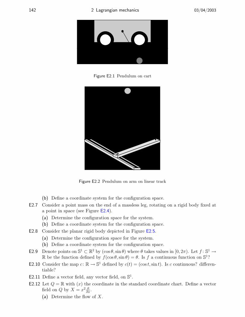
142 2 Lagrangian mechanics 03/04/2003
Figure E2.1 Pendulum on cart
Figure E2.2 Pendulum on arm on linear track
(b) Define a coordinate system for the configuration space.
E2.7 Consider a point mass on the end of a massless leg, rotating on a rigid body fixed ata point in space (see Figure E2.4).
(a) Determine the configuration space for the system.
(b) Define a coordinate system for the configuration space.
E2.8 Consider the planar rigid body depicted in Figure E2.5.
(a) Determine the configuration space for the system.
(b) Define a coordinate system for the configuration space.
E2.9 Denote points on S1 ⊂ R2 by (cos θ, sin θ) where θ takes values in [0, 2π). Let f : S1 →R be the function defined by f(cos θ, sin θ) = θ. Is f a continuous function on S1?
E2.10 Consider the map c : R → S1 defined by c(t) = (cos t, sin t). Is c continuous? differen-tiable?
E2.11 Define a vector field, any vector field, on S1.
E2.12 Let Q = R with (x) the coordinate in the standard coordinate chart. Define a vectorfield on Q by X = x2 ∂
∂x.
(a) Determine the flow of X.

Exercises for Chapter 2 143
Figure E2.3 A two-axis gyroscope
Figure E2.4 A “robotic leg”
Figure E2.5 A planar rigid body

144 2 Lagrangian mechanics 03/04/2003
Now consider another coordinate chart (V, ψ) for Q defined V = Q and ψ(x) = ex.
(b) Express X in this new coordinate chart.
(c) Determine the flow of X in this new coordinate chart.
E2.13 Is it possible to define two vector fields X1 and X2 on S2 with the property thatX1(q), X2(q) are linearly independent for every q ∈ Q?
E2.14 Let Q = R2 with (x, y) the coordinates in the standard coordinate chart. Define avector field on Q by X = x ∂
∂x+ y ∂
∂y.
(a) Determine the flow of X.
(b) Determine the components of X in the polar coordinate chart.
(c) Determine the flow of X in the polar coordinate chart.
E2.15 Let Q be a configuration space with (U, φ) a coordinate chart. For vector fields Xand Y with components (X1, . . . , Xn) and Y 1, . . . , Y n) in the given chart, we proposethe following two expressions,
∂Y i
∂qjXj +
∂X i
∂qjY j, i = 1, . . . , n,
∂Y i
∂qjXj − ∂X i
∂qjY j, i = 1, . . . , n,
as being the components of a vector field on Q. Which, if either, are actually thecomponents of a vector field?
E2.16 When we allow arbitrary coordinate charts, the notion of a linear ordinary differentialequation looses its distinctness. Let Q = R2 and consider on Q with the standardcoordinate system (U1, φ1) defined in the usual manner by U1 = R2 and φ1(x, y) =(x, y). In these coordinates define a vector field
X = x∂
∂x− y
∂
∂x.
(a) Determine the flow of X.
Now consider the coordinate chart (U2, φ2) where U2 = R2 and φ2(x, y) = ().Finish this
(b) Write the vector field X in this coordinate chart.
(c) Obtain the flow in these coordinates. Do you think you could have solved the dif-ferential equations were you given them without knowing how they came about?
E2.17 Let Q be a configuration space with g a Riemannian metric on Q. Show that for acoordinate chart (U, φ) with coordinates (q1, . . . , qn) and for a fixed q ∈ U , the linearmap g[(q) : TqQ→ T ∗q Q has components gij, i, j = 1, . . . , n, with respect to the bases
∂∂q1
∣∣q, . . . , ∂
∂q1
∣∣q and dq1|q, . . . , dqn|q for TqQ and T ∗q Q, respectively. Also show
that the components of g](q) : T ∗q Q → TqQ with respect to these same bases are gij,i, j = 1, . . . , n.
E2.18 Let c ∈ C2([a, b], qa, qb) and let [t1, t2] ⊂ [a, b]. Let c ∈ C2([t1, t2], c(t1), c(t2)) anddefine a curve c1 : [a, b] → Q by
c1(t) =
c(t), t ∈ [a, t1]
c1(t), t ∈ [t1, t2]
c(t), ∈ [t2, b].

Exercises for Chapter 2 145
Show that for any ε > 0 there exists a curve c1 ∈ C2([a, b], qa, qb) so that|JL(c1)− JL(c1)| ≤ ε.Hint: You may find it helpful to use a function like
f(x) =
exp(−1/(1− x2)), −1 < x < 1
0, otherwise.
E2.19 For the system of Exercise E2.4 do the following.
(a) Determine the kinetic energy Riemannian metric for the system in your set ofcoordinates.
(b) Determine the Christoffel symbols for the Riemannian metric.
(c) Determine the potential function.
(d) Using this data, write the Euler-Lagrange equations for the system.
E2.20 For the system of Exercise E2.5 do the following.
(a) Determine the kinetic energy Riemannian metric for the system in your set ofcoordinates.
(b) Determine the Christoffel symbols for the Riemannian metric.
(c) Determine the potential function.
(d) Using this data, write the Euler-Lagrange equations for the system.
E2.21 For the system of Exercise E2.6 do the following.
(a) Determine the kinetic energy Riemannian metric for the system in your set ofcoordinates.
(b) Determine the Christoffel symbols for the Riemannian metric.
(c) Determine the potential function.
(d) Using this data, write the Euler-Lagrange equations for the system.
E2.22 For the system of Exercise E2.7 do the following.
(a) Determine the kinetic energy Riemannian metric for the system in your set ofcoordinates.
(b) Determine the Christoffel symbols for the Riemannian metric.
(c) Determine the potential function.
(d) Using this data, write the Euler-Lagrange equations for the system.
E2.23 For the system of Exercise E2.8 do the following.
(a) Determine the kinetic energy Riemannian metric for the system in your set ofcoordinates.
(b) Determine the Christoffel symbols for the Riemannian metric.
(c) Determine the potential function.
(d) Using this data, write the Euler-Lagrange equations for the system.
E2.24 Exercise on how the Newtonian potential gives the linear approximation.
E2.25 Let Q = R and let F : R × TQ → T ∗Q be a force which is independent of time andvelocity. Show that F is a potential force. Show that this is not true when Q = R2.
E2.26 Let ∇ be an affine connection on a configuration space Q and let (U1, φ1) and (U2, φ2)be overlapping coordinate charts with coordinates (q1, . . . , qn) and (q1, . . . , qn). If Γi
jk,i, j, k = 1, . . . , n are the Christoffel symbols for ∇ in the coordinate chart (U1, φ1)

146 2 Lagrangian mechanics 03/04/2003
and Γijk, i, j, k = 1, . . . , n, are the Christoffel symbols for ∇ in the coordinate chart
(U2, φ2), show that
Γijk =
∂qi
∂q`
∂qr
∂qj
∂qs
∂qkΓ`
rs +∂qi
∂q`
∂2q`
∂qj∂qk.
Show that as a result of this, the geodesic equations
qi + Γijkq
j qk = 0, i = 1, . . . , n,
are independent of coordinates. What can you say about the coordinate independenceof each of the separate terms “qi” and “Γi
jkqj qk” in the geodesic equation?
E2.27 Argue that the quantity defined in equation (2.14) generalises the usual freshmannotion of “work.”
E2.28 Let Q = R2 \ (0, 0) and define a force on Q by
F (t, x, y, vx, vy) = − y
x2 + y2dx+
x
x2 + y2dy.
(a) Is F a potential force? Why or why not?
(b) If Q = (x, y) ∈ Q | x > 0, if F a potential force on Q? Why or why not?
E2.29 This is a continuation of Exercise E2.4. Suppose that a torque is applied to the baseof the pendulum. What is this force, written as a one-form on Q?
E2.30 This is a continuation of Exercise E2.5. Suppose that two forces are applied to thesystem, one a torque at the base of the arm to rotate the arm, and the other a linearforce moving the base down the track. What are these forces, written as a one-formson Q?
E2.31 This is a continuation of Exercise E2.6. Suppose that a torque is applied which rotatesthe gyro in its frame. What is this force, written as a one-form on Q?
E2.32 This is a continuation of Exercise E2.7. Suppose that we actuate the system with twoinputs as follows. We may apply a linear force to the mass, so extending its distancefrom the pivot, and we have a motor atop the rigid body which we can use to actuatethe angle of the arm relative to the body. What are these forces, written as one-formson Q?
E2.33 This is a continuation of Exercise E2.8. Suppose a force F is applied to the body ata point a distance h form the centre of mass. Write this force as a one-form on Q.
E2.34 Show using Frobenius’s theorem that if C is a linear constraint with the property thatrank(C) = 1, then C is holonomic.
E2.35 Let C be a constraint on Q and let the one-forms α1, . . . , αn−r be a basis for ann(`(C)).Show that the vector fields g](α1), . . . , g](αn−r) form a basis for `(C)⊥.
E2.36 Consider a ball rolling on a flat horizontal table rotating with uniform angular velocityΩ with respect to some inertial frame (see Figure E2.6).
(a) What is the configuration space for the system?
Suppose that the ball has radius r, mass m, and isotropic inertia tensor so that allprincipal inertias are equal to I.
(b) Use the spatial angular velocity ω of the ball to express the constraints of thesystem.

Exercises for Chapter 2 147
Ω
(x, y)
Figure E2.6 Ball rolling on rotating table
(c) Using the definition of the spatial angular velocity, turn the constraints from theprevious part of the problem into a constraint of the type we discuss. Is theconstraint linear? Why or why not?
(d) Write the Lagrangian for the system in terms of the spatial angular velocities.
(e) Use the previous part of the problem, give an expression for the Lagrangian as afunction on the tangent bundle of the configuration space. Use Exercise E1.11(e)to make for a nicer expression of the rotational kinetic energy.
You will observe that this Lagrangian is not altogether a pleasant one, and that writingthe Euler-Lagrange equations is not a pleasing prospect.
(f) However, use the fact that the Euler-Lagrange equations are equivalent to New-ton’s equations to obtain the equations of motion in terms of the spatial angularvelocities and the position of contact of the ball with the table.
E2.37 Show that the body angular velocity of a rigid body is not a vector in the tangentspace to the configuration space Q = SO(3).
E2.38 Let Q be a configuration space and consider a function H : R × T ∗Q → R. In acoordinate chart, define a map FH : R× T ∗Q→ R× TQ by
FH(t, q,p) =(q,∂H
∂p
).
(a) Show that FH is well-defined, i.e., that the above definition is independent ofcoordinates, and that FH(t, αq) ∈ TqQ.
Call the function H hyperregular if FH is a diffeomorphism. For a hyperregularH, define a function LH : R× TQ→ R by
LH(t, vq) = 〈FH−1(vq); vq〉 −H(t,FH−1(vq)).
(b) State and prove the natural result corresponding to Theorem 2.9.2.
(c) Show that for a hyperregular Lagrangian, HL is a hyperregular Hamiltonian andthat FL−1 = FHL.
(d) Show that for a hyperregular Hamiltonian, LH is a hyperregular Lagrangian andthat FH−1 = FLH .

148 2 Lagrangian mechanics 03/04/2003

This version: 03/04/2003
Chapter 3
Lagrangian dynamics
Essentially, the previous two chapters dealt with writing the equations of motion, andhad very little to say about the behaviour of the solutions of the resulting equations. Gen-erally, one can say very little about the nature of solutions to the Euler-Lagrange equations.Therefore, in this section we look at special cases, and introduce qualitative methods. Thestudy of the dynamics of mechanical systems fills an enormous number of pages, but despitethis, very little is known about the behaviour of such systems. Thus we start our discussionin this section with some rather general ideas. Only when we get to Section 3.4 are we able toapply the general ideas to specific, and very simple, systems. It is only in these very specialcases that one is able approach anything like a complete understanding to the dynamics ofa class of systems. For these systems, the general ideas of the earlier sections of the chapterbecome more tangible, so it is hoped that the reader will have some patience in waiting forthe application of these ideas.
3.1 The Euler-Lagrange equations and differential equations
We begin our investigation of Lagrangian dynamics with a discussion of how one obtainsdifferential equations from the Euler-Lagrange equations. For those who think that theEuler-Lagrange equations are differential equations, we bring you the following example.
3.1.1 Example Consider the Lagrangian on Q = R defined by L(t, x, v) = v − x. The Euler-Lagrange equation (there is only one) is then
d
dt
(∂L∂v
)− ∂L
∂x= 1 = 0.
Clearly this is nonsense, and in this case there can be no solution for the Euler-Lagrangeequations.
You will say that the preceding example is contrived, as surely it is. However, it nonethe-less points out the need for there to be some consideration given to the matter of when theEuler-Lagrange equations have solutions. The following result is perhaps not surprisinggiven Theorem 2.9.2.
3.1.2 Proposition If L is a hyperregular Lagrangian on Q, then for each q0 ∈ Q and foreach v0 ∈ Tq0Q there exists T > 0 and a solution c : [t0, t0 + T] → Q to the Euler-Lagrangeequations for L with the property that c′(t0) = v0. Furthermore, if we have T > 0 anda curve c : [t0, t0 + T] → Q with the properties that c is a solution to the Euler-Lagrangeequations and that c′(t0) = v0, then c(t) = c(t) for all t ∈ [t0, t0 + T] ∩ [t0, t0 + T].

150 3 Lagrangian dynamics 03/04/2003
Proof We fix a coordinate chart (U, φ) around q. Since L is hyperregular, the map FL,given in coordinates by,
(q1, . . . , qn, v1, . . . , vn) 7→(q1, . . . , qn,
∂L
∂v1, . . . ,
∂L
∂vn
)is invertible. By the inverse function theorem, this means that the Jacobian of the map mustalso be invertible. The Jacobian will be a matrix of the form[
In 0n×n
A1 A2
],
where A1 is the matrix with components ∂2L∂vi∂qj , i, j = 1, . . . , n, and where A2 is the matrix
with components ∂2L∂vi∂vj , i, j = 1, . . . , n. In order that this Jacobian be invertible, it is
necessary and sufficient that A2 be invertible when evaluated at any (q,v) ∈ Rn × Rn.Now let us look at the Euler-Lagrange equations. We expand them to arrive at
d
dt
( ∂L∂vi
)− ∂L
∂qi=
∂2L
∂vi∂vjvj +
∂2L
∂vi∂qjqj +
∂2L
∂vi∂t− ∂L
∂qi, i = 1, . . . , n.
Therefore, the Euler-Lagrange equations, when L is hyperregular, are equivalent to
qk =(A−1
2
)ki(∂L∂qi
− ∂2L
∂vi∂qjqj − ∂2L
∂vi∂t
), k = 1, . . . , n.
Here(A−1
2
)ki, k, i = 1, . . . , n, are the components of the inverse of A2. Thus we have shown
that the Euler-Lagrange equations are equivalent to a second-order differential equationwhen the Lagrangian is hyperregular, and thus the result follows by the standard existenceand uniqueness theory for ordinary differential equations.
The above result has the following corollary which gets us out of the woods as concernsworrying about existence and uniqueness of solutions for simple mechanical systems.
3.1.3 Corollary If (Q, g,V) is a simple mechanical system with Lagrangian L, then for eachq0 ∈ Q and for each v0 ∈ Tq0Q there exists T > 0 and a solution c : [t0, t0 + T] → Q to theEuler-Lagrange equations for L with the property that c′(t0) = v0. Furthermore, if we haveT > 0 and a curve c : [t0, t0 + T] → Q with the properties that c is a solution to the Euler-Lagrange equations and that c′(t0) = v0, then c(t) = c(t) for all t ∈ [t0, t0 + T]∩ [t0, t0 + T].
Proof This follows directly from Proposition 2.9.1.
Also note that the differential equations derived in Proposition 2.4.5 for simple mechanicalsystems also serve as proof of the previous result. In any case, the bottom line is that theequations describing the behaviour of simple mechanical systems, at least in the absenceof forces and constraints, satisfy the usual existence and uniqueness properties of ordinarydifferential equations.
Let us explore this just a little bit further in order that we ensure ourselves that we haveleft some stones unturned. Indeed, the immediate question raised by Proposition 3.1.2 iswhether hyperregularity of L is equivalent to there being a unique solution to the Euler-Lagrange equations through each point vq ∈ TQ. The answer is that while hyperregularityis, as we have seen, sufficient for existence and uniqueness, it is not necessary. Some contrivedexamples illustrate this.

03/04/2003 3.2 Linearisations of Lagrangian systems 151
3.1.4 Examples 1. On Q = R consider the Lagrangian L(t, x, v) = ev. This Lagrangian isnot hyperregular since the Legendre transformation
(x, v) 7→ (x, ev)
is not surjective; points of the form (x, a) are not in the image of the Legendre transfor-mation when a < 0. However, the Euler-Lagrange equation is determined to be exx = 0,which is clearly equivalent to x = 0. Thus the Euler-Lagrange equations possess uniquesolutions for any initial condition, despite the Lagrangian not being hyperregular.
2. On Q = R consider the Lagrangian L(t, x, v) = xv. One determines that the Euler-Lagrange equations are then simply 0 = 0. In this case, any function of t will be asolution! Thus, the Euler-Lagrange equations possess solutions, but they are not unique.
3. Example where
injective
The above examples suggest that if we are unwilling to place restrictions on our La-grangians, we can expect the Euler-Lagrange equations to be generally weird. However,Corollary 3.1.3 assures us that if we are dealing with typical Lagrangians from physics, thenthings are as they are in the standard theory of differential equations.
3.2 Linearisations of Lagrangian systems
The first thing one does with pretty much any general ordinary differential equation isseek fixed points, and linearise about them. This is a good idea for Lagrangian systemsas well, and as we shall see, linearisation of Lagrangian systems yields a structure which isquite special.
3.2.1 Linear Lagrangian systems When we linearise a general differential equation,the linearisation of the system is, by construction, a linear differential equation. Similarly,when we linearise Euler-Lagrange equations, we end up with “linear Euler-Lagrange equa-tions.” Therefore, it is helpful to know what these are.
In order to define the equations governing the behaviour of a linear Lagrangian system,it is helpful to have at hand some notation. Let V be a R-vector space (let us agree notto confuse V in this discussion with the potential function V ). A map A : V × V → R isbilinear if
A(u1 + u2, v1 + v2) = A(u1, v1) + A(u1, v2) + A(u2, v1) + A(u2, v2)
for all u1, u2, v1, v2 ∈ V and ifA(au, bv) = abA(u, v)
for all a, b ∈ R and u, v ∈ V . A bilinear map A is symmetric (resp. skew-symmetric)if A(u, v) = A(v, u) (resp. A(u, v) = −A(v, u)) for all u, v ∈ V . We all know of an exampleof a symmetric bilinear map, and that is an inner product which further has the propertythat A(u, u) > 0 for u 6= 0. Using our notation for inner products as motivation, for asymmetric bilinear map A : V × V → R define a map A[ : V → V ∗ by asking that A(u)satisfy
⟨A[(u); v
⟩= A(u, v). If e1, . . . , en is a basis for V with dual basis e1, . . . , en
for V ∗, then the matrix of A in the given basis is defined to be the n × n matrix withcomponents
Aij = A(ei, ej), i, j = 1, . . . , n.

152 3 Lagrangian dynamics 03/04/2003
Note, of course, that Aij = Aji, i, j = 1, . . . , n. One then readily verifies (see, for example,Exercise E2.17) that
A(viei) = Aijviej,
thus giving a component expression for A[. If A is skew-symmetric, then one may defineA[ : V → V ∗ in exactly the same way, except that the matrix with components Aij, i, j =1, . . . , n, will now be skew-symmetric.
Now we may make our definition concerning linear Lagrangian systems.
3.2.1 Definition Let V be an n-dimensional R-vector space. A linear Lagrangian systemon V is a triple (M,C,K) where M,C,K : V × V → R are bilinear maps with M and Kbeing symmetric and C being skew-symmetric. The Lagrangian associated with a linearLagrangian system (M,C,K) is the function L : V × V → R defined by
L(u, v) =1
2M(v, v) +
1
2C(u, v)− 1
2K(u, u).
A curve t 7→ c(t) ∈ V is a solution of the linear Lagrangian system (M,C,K) if c satisfiesthe differential equation
M [(c(t)) + C[(c(t)) +K[(c(t)) = 0.
Note that our notion of a solution for a linear Lagrangian system seems disjointed fromthe usual notion of solutions for Euler-Lagrange equations. Let us state a result to makethe connection. In stating the result, it is helpful to note that for a R-vector space V wehave TV ' V × V . We shall simply state this as a fact, and not prove it, although thisis easily done in an appropriate setting. Using this fact, a point vq in TV is written as(q, v) ∈ V × V .
3.2.2 Proposition Let V be a R-vector space and let (M,C,K) be a linear Lagrangian systemon V with Lagrangian L defined on V × V ' TQ. A curve t 7→ c(t) ∈ V is a solution tothe linear Lagrangian system (M,C,K) if and only if it is a solution to the Euler-Lagrangeequations for L.
Proof We have
L(q, v) =1
2M(v, v) +
1
2C(q, v)− 1
2K(q, q).
Let e1, . . . , en be a basis for V with Mij, Cij, and Kij, i, j = 1, . . . , n, the matrices for M ,C, and K in this basis. We compute
d
dt
( ∂L∂vi
)− ∂L
∂qi= Mjiq
j +1
2Cjiq
j − 1
2Cij q
j +Kjiqj, i = 1, . . . , n.
The result now follows since Cji = −Cij, i, j = 1, . . . , n.
In the case when M is invertible then its inverse is denoted M ] : V ∗ → V . Also, in thiscase we may write the equations which are satisfied by a linear Lagrangian system as thefollowing set of 2n first-order differential equations:(
qv
)=
[0 idV
−M ] K[ −M ] C[
](qv
),

03/04/2003 3.2 Linearisations of Lagrangian systems 153
where idV is the identity map on V . Note that M ] K[ and M ] C[ are simply lineartransformations of V . Recall that the behaviour of the linear system is determined in largepart by the eigenvalues of the linear transformation A(M,C,K) : V × V → V × V which isrepresented by
A(M,C,K) =
[0 idV
−M ] K[ −M ] C[
].
The following result characterises these eigenvalues.
3.2.3 Proposition Let (M,C,K) be a linear Lagrangian system on a vector space V, andsuppose that M[ is invertible. If λ ∈ C is an eigenvalue of A(M,C,K) then
(i) −λ is an eigenvalue of A(M,C,K);
(ii) λ is an eigenvalue of A(M,C,K);
(iii) −λ is an eigenvalue of A(M,C,K);
Furthermore, the multiplicity of the eigenvalues λ, −λ, λ, and −λ are equal.
Proof On the vector space V 2 = V × V define a bilinear map JM,C : V 2 × V 2 → R by
JM,C((u1, u2), (v1, v2)) = M(u1, v2)−M(u2, v1) + C(v1, u1).
Clearly J is skew-symmetric. If M [ is invertible then JM,C is nondegenerate in the sensethat if JM,C((u1, u2), (v1, v2)) = 0 for all (v1, v2) ∈ V 2, then (u1, u2) = (0, 0). Indeed, ifJM,C((u1, u2), (v1, v2)) = 0 for all (v1, v2) ∈ V 2 then
M(u1, v2)−M(u2, v1) = 0
for all (v1, v2) ∈ V 2. Taking v1 = 0, this means that M(u1, v2) =⟨M [(u1); v2
⟩= 0 for all
v2 ∈ V . This implies that M [(u1) = 0 and since M [ is invertible, this means that u1 = 0.Taking v2 = 0 we see that we must have M(u2, v1)− C(v1, u1) = 0 for every v1 ∈ V . Sinceu1 has already been demonstrated to be zero, it follows that M(u2, v1) =
⟨M [(u2); v1
⟩= 0
for every v1 ∈ V , from which we deduce that u2 = 0.Next we compute
JM,C(A(M,C,K)(u1, u2), (v1, v2))
= JM,C((u2,−M ] K[(u1)−M ] C[(u2)), (v1, v2)) + C(v1, u2)
= M(u2, v2) +M(M ] K[(u1) +M ] C[(u2), v1) + C(v1, u2)
= M(u2, v2) +K(u1, v1) + C(u2, v1) + C(v1, u2)
= M(v2, u2) +K(v1, u1) + C(v2, u1)− C(v2, u1)
= M(M ] K[(v1) +M ] C[(v2), u1) +M(v2, u2)− C(v2, u1)
= −M(u1,−M ] K[(v1)−M ] C[(v2)) +M(v2, u2)− C(v2, u1)
= − JM,C((u1, u2), (v2,−M ] K[(v1)−M ] C[(v2))
= − JM,C((u1, u2), A(M,C,K)(v1, v2)).
Let us now use this fact to prove the result.Suppose that λ ∈ C is an eigenvalue as stated. Then there exists a vector v = (v1, v2) ∈
V 2 so that A(M,C,K)(v) = λv. This means that for every v ∈ V 2 we have
JM,C(v, A(M,C,K)(v)− λv) = 0
=⇒ − JM,C(A(M,C,K)(v), v)− λJM,C(v, v) = 0
=⇒ JM,C((A(M,C,K) + λ idV 2)v, v) = 0.
(3.1)

154 3 Lagrangian dynamics 03/04/2003
This proves that is v is an eigenvector for A(M,C,K) with eigenvalue λ then v is orthogonalto image(A(M,C,K) +λ idV 2) with orthogonality taken with respect to JM,C . This renders thefollowing lemma helpful.
1 Lemma Let U be a finite-dimensional R-vector space with J: U×U → R a nondegenerateskew-symmetric bilinear map. For a linear map B: U → U define B : U → U by
J(B(u1), u2) = J(u1,B(u2)).
Then the following facts hold:
(i) a vector u ∈ U satisfies J(B(u), u) = 0 for every u ∈ U if and only if u ∈ ker(B)—thatis, the J-orthogonal complement to image(B) is equal to ker(B);
(ii) dim(ker(B)) = dim(ker(B)).
Proof (i) We haveu ∈ U
∣∣ J(B(u), u) = 0 for every u ∈ U
=u ∈ U
∣∣ J(u, B(u)) = 0 for every u ∈ U
=u ∈ U
∣∣ B(u) = 0
= ker(B).
(ii) Choose a basis u1, . . . , um for V . Let Jij, i, j = 1, . . . ,m, be the matrix for J in this
basis, let Bij, i, j = 1, . . . ,m, be the matrix for B in this basis, and let Bi
j, i, j = 1, . . . ,m,
be the matrix for B in this basis. We then have, by the definition of B,
JkiBkj = JjkB
ji , i, j = 1, . . . ,m.
Letting J ij, i, j = 1, . . . ,m, be the components of the inverse of the matrix with componentsJij, i, j = 1, . . . ,m, we then have
Bij = JkiB`
kJj`, i = 1, . . . , n.
Writing this in matrix form, it reads B = J−tBJ t. Now since J is nondegenerate, J isinvertible, which implies that B and B have the same rank. H
Using the lemma with U = V 2, J = JM,C , and B = A(M,C,K) + λ idV 2 , we see that if v is aneigenvector for A(M,C,K) with eigenvalue λ then v ∈ ker((A(M,C,K) + λ idV 2)∧). Also by thelemma, this implies that there exists a nonzero vector v′ ∈ ker(A(M,C,K) + λ idV 2), and thusv′ is an eigenvector with eigenvalue −λ. That λ and −λ are eigenvalues follows from thefact that V is a real vector space.
For the final assertion of the proposition, note that the reasoning of (3.1), along withpart (i) of the above lemma, demonstrates that
dim(ker(A(M,C,K) − λ idV 2)) = dim(ker((A(M,C,K) − λ idV 2)∧)),
and so the assertion about the multiplicities then follows from part (ii) of the above lemma.
3.2.4 Remark The above proof, although straightforward in nature, relies on the introductionof the mysterious bilinear map JM,C . This may seem like something of a rabbit pulled froma hat, and indeed it is without some extra context. On the R-vector space V × V ∗ considerthe skew-symmetric bilinear map J : (V × V ∗)2 → R defined by
J((v1, α1), (v2, α
2)) = α2(v1)− α1(v2).

03/04/2003 3.2 Linearisations of Lagrangian systems 155
Note that this map is defined without the assistance of additional structure. Now consider alinear Lagrangian system (M,C,K) on V . The Legendre transformation for the correspond-ing Lagrangian L is the map
FL(q, v) = (q,M [(v) + 12C[(q)).
The map JM,C defined in the proof of Proposition 3.2.3 is readily determined to be exactly
JM,C((u1, u2), (v1, v2)) = J(FL(u1, u2),FL(v1, v2)).
Thus JM,C is “the same” as J . The object J is well studied, and is called a symplecticstructure on the vector space V × V ∗. The mapping A(M,C,K) is then an example of aninfinitesimally symplectic mapping . These are well studied, and here we only give aglimpse of their properties. Williamson [1937] gives a classification of the Jordan normalforms for such linear mappings.
The position of the eigenvalues for various situations is shown in Figure 3.1. Let us
λ
λ
−λ λ
−λ λ
−λ λ
Figure 3.1 Imaginary eigenvalues (left), real eigenvalues (middle),and general complex eigenvalues (right) for a linear Lagrangiansystem
illustrate the conclusions of Proposition 3.2.3 in the simplest possible case.
3.2.5 Example We take V = R and define a linear mechanical system on V by M = m,C = 0, K = k, for m, k ∈ R. Note that skew-symmetric linear mappings on a 1-dimensionalvector space are necessarily zero. We then have, provided that m 6= 0,
A(M,C,K) =
[0 1− k
m0
].
We have three cases.
1. If km
is positive, then we write km
= ω20. The eigenvalues of A(M,C,K) are readily computed
to be λ1 = iω0 and λ2 = −iω0. Thus, in this case, both eigenvalues are purely imaginary,and they obviously have the property of being complex conjugates of one another.
2. If km
is negative, that we write km
= −ω20 and we determine that the eigenvalues of
A(M,C,K) are λ1 = ω0 and λ2 = −ω0. Thus we see that when we have a real eigenvalue,we also have its negative, as predicted by Proposition 3.2.3.
3. The final case is when km
= 0 when the eigenvalues are both zero. These also obviouslysatisfy the conditions of Proposition 3.2.3.

156 3 Lagrangian dynamics 03/04/2003
Let us finally address the question of what are the implications of Proposition 3.2.3 forthe dynamics of linear Lagrangian systems, at least when M [ is invertible.
The reader will at this point wish to recall some of the basic ideas assembled in Section C.2concerning fixed points of general ordinary differential equations. In particular, we will atthis point make reference to the notions of stability and asymptotic stability of a fixed point.
Recall that the algebraic multiplicity of an eigenvalue is the multiplicity of the eigen-value as a root of the characteristic polynomial, and that the geometric multiplicity of aneigenvalue is the dimension of the eigenspace for that eigenvalue. The algebraic multiplicityalways bounds the geometric multiplicity from above. The following result gives the stabilityproperties of a linear Lagrangian system. The proof relies on some elementary facts fromthe theory of linear differential equations with constant coefficients. A rapid review of thismaterial may be found in Section C.1. The notions of stability we use are to be found inSection C.2.
3.2.6 Proposition Let (M,C,K) be a linear Lagrangian system on a vector space V and sup-pose that M[ is invertible. Consider the differential equation(
qv
)=
[0 idV
−M] K[ −M] C[
](qv
). (3.2 )
A point (q0, v0) ∈ V2 is a fixed point of (3.2) if and only if v0 = 0 and q0 ∈ ker(K]).Let (q0, v0) be a fixed point of (3.2). The following statements hold:
(i) (q0, v0) is not asymptotically stable;
(ii) (q0, v0) is stable if and only if all eigenvalues of A(M,C,K) lie on the imaginary axis andhave equal algebraic and geometric multiplicities.
Proof That (q0, v0) ∈ V 2 is a fixed point of (3.2) if and only if v0 = 0 and q0 ∈ ker(K])follows directly from the form of A(M,C,K).
(i) This follows since a linear system is asymptotically stable if and only if all eigenvalueshave negative real part. For a linear Lagrangian system, if an eigenvalue has negative realpart, then Proposition 3.2.3 guarantees that there will also be an eigenvalue with positivereal part.
(ii) From part (i) we see that for a fixed point to be stable, all eigenvalues of A(M,C,K)
should lie on the imaginary axis. Recall from the Jordan canonical form theorem that if thegeometric multiplicity is less than the algebraic multiplicity, then for some initial conditionsthe solution will have the form of a linear combination of terms like
tk cosωt, tk sinωt,
for some ω ≥ 0 and k ≥ 1. This precludes stability as such solutions are not bounded ast→∞.
Our previous simple example is enough to illustrate the consequences of the previousresult.
3.2.7 Example (Example 3.2.5 cont’d) We again take V = R and take the linear Lagrangiansystem with M = m, C = 0, and K = k. We had
A(M,C,K) =
[0 1− k
m0
].

03/04/2003 3.2 Linearisations of Lagrangian systems 157
Recall that the solution to (3.2) is(q(t)v(t)
)= eA(M,C,K)t
(q(0)v(0)
).
Again, we consider three cases.
1. We first take km> 0 and write k
m= ω2
0. In this case, the only fixed point is (0, 0) sinceK] is invertible. A straightforward computation gives
eA(M,C,K)t =
[cos(ω0t)
sin(ω0t)ω0
−ω0 sin(ω0t) cos(ω0t)
].
Clearly, by choosing the initial condition small enough, one can ensure that solutionsremain inside a ball of any specified radius. Thus (0, 0) is a stable fixed point. However,it is not asymptotically stable.
2. Next take km< 0 and write k
m= −ω2
0. Again the only fixed point is (0, 0). One alsocomputes
eA(M,C,K)t =
[cosh(ω0t)
sinh(ω0t)ω0
−ω0 sinh(ω0t) cosh(ω0t)
].
Note that now there will be initial conditions which result in unbounded solutions. There-fore, the system is not stable.
3. Finally we take k = 0. In this case any point (q0, 0) will be a fixed point since K = 0.One computes
eA(M,C,K)t =
[1 t0 1
].
Therefore any initial condition with v(0) 6= 0 will result in unbounded solutions. Thisprecludes any of the infinite number of fixed points from being stable. Note here thatthe eigenvalues lie on the imaginary axis—they are both zero—but since the geometricmultiplicity is only one, Proposition 3.2.6 implies that fixed points will be unstable.
3.2.8 Remark We have studiously avoided talking about the case when M ] is not invertible.In such cases, the differential equations
Mq + Cq +Kq = 0
are “implicit” in that one cannot solve explicitly for the derivative and stick it on the left-hand side as one likes to do with differential equations. In this situation, the concerns ofSection 3.1 come into play. That is to say, matters of existence and uniqueness become ofconcern. Rather than getting involved in such matters, we will concentrate on describing thedynamics in those cases when the Euler-Lagrange equations give well-behaved differentialequations.
3.2.2 Equilibria for Lagrangian systems In order to linearise, we need something tolinearise about, and such things are titled “equilibria.” To be specific, let L be a Lagrangianon a configuration space Q. A point q0 ∈ Q is an equilibrium point for L if the trivialcurve t 7→ q0 is a solution of the Euler-Lagrange equations for L. The following result givesa useful characterisation of equilibrium points for time-independent Lagrangians. For thestatement of this result, we use the notation 0q to denote the zero vector in the tangentspace TqQ.

158 3 Lagrangian dynamics 03/04/2003
3.2.9 Proposition A point q0 is an equilibrium point for a time-independent Lagrangian L ona configuration space Q if and only if dEL(0q0) = 0.
Proof We work in a set of coordinates (q1, . . . , qn) and denote by q0 the image of q0 in thisset of coordinates. Recall that in coordinates we have
EL =∂L
∂vivi − L
so that
dEL =∂2L
∂qj∂vividqj +
∂2L
∂vj∂vividvj +
∂L
∂vidvi − ∂L
∂qidqi − ∂L
∂vidvi
=∂2L
∂qj∂vividqj +
∂2L
∂vj∂vividvj − ∂L
∂qidqi.
Thus dEL(0q0) = 0 if and only if
∂L
∂qi(q0,0) = 0, i = 1, . . . , n. (3.3)
However, this Euler-Lagrange equations are
∂2L
∂vj∂viqj +
∂2L
∂qj∂viqj − ∂L
∂qi= 0, i = 1, . . . , n.
Thus q0 is an equilibrium point if and only if (3.3) holds, and thus follows the proposition.
This fact relating the energy to equilibrium points will be important when we talk aboutdynamics near equilibrium points later in this section.
We shall now in show that when the Lagrangian is time-independent, one may define alinear Lagrangian system on the vector space Tq0Q. Suppose that L is a time-independentLagrangian on a configuration space Q and let q0 ∈ Q be an equilibrium point for L. Letus choose a coordinate chart (U, φ) around q0 with coordinates (q1, . . . , qn), and supposethat φ(q0) = q0. Let us try to obtain an approximate expression for solutions of the Euler-Lagrange equations which start near q0. Let t 7→ q(t) be a coordinate representation of sucha solution. We therefore have the Euler-Lagrange equations:
d
dt
( ∂L∂vi
)− ∂L
∂qi= 0, i = 1, . . . , n.
Let us Taylor expand everything about (q,v) = (q0,0). We have
d
dt
( ∂2L
∂qj∂vi(qj(t)− qj
0) +∂2L
∂vj∂vi(qj(t)− qj
0) + · · ·)−
∂2L
∂qj∂qj(qj(t)− qj
0)−∂2L
∂vj∂qi(qj(t)− qj
0) + · · · = 0
=⇒ ∂2L
∂vj∂viξj(t) +
( ∂2L
∂qj∂vi− ∂2L
∂vj∂qi
)ξj(t)− ∂2L
∂qj∂qiξj(t) + · · · = 0,
where ξi(t) = qi(t)−qi0, i = 1, . . . , n. Here all partial derivatives have been evaluated at each
step at (q0,0), and we have used the fact that t 7→ q0 is a solution of the Euler-Lagrange

03/04/2003 3.2 Linearisations of Lagrangian systems 159
equations. From this expression we may define a linear Lagrangian system (ML,CL,KL)on Rn by asking that the matrix representations of these bilinear maps satisfy
(ML)ij =∂2L
∂vi∂vj(q0,0), i, j = 1, . . . , n
(CL)ij =∂2L
∂qi∂vj(q0,0)− ∂2L
∂vi∂qj(q0,0), i, j = 1, . . . , n
(KL)ij = − ∂2L
∂qi∂qj(q0,0), i, j = 1, . . . , n.
(3.4)
This is, of course, not very satisfying because it only works in a fixed coordinate chart. Thefollowing result indicates how that can be made to be coordinate independent.
3.2.10 Proposition Let L be a time-independent Lagrangian on Q and let q0 be an equilibriumpoint for L. There exists bilinear maps ML(q0),CL(q0),KL(q0) : Tq0Q × Tq0Q → R withML(q0) and KL(q0) symmetric, and with CL(q0) skew-symmetric, and having the propertythat with respect to any set of coordinates (q1, . . . , qn) they are represented as in (3.4).
Proof Let (q1, . . . , qn) and (q1, . . . , qn) be two sets of coordinates around q0. Suppose thatq0 is mapped to q0 and q0 in the two sets of coordinates. Using the chain rule and evaluatingat (q0,0) we compute
∂2L
∂vi∂vj(q0,0) =
( ∂2L
∂vk∂v`
∂qk
∂qi
∂q`
∂qj
)(q0,0)
∂2L
∂qi∂vj(q0,0) =
( ∂2L
∂q`∂vk
∂q`
∂qi
∂qk
∂qj
)(q0,0) +
( ∂L∂vk
∂2qk
∂qi∂qj
)(q0,0)
∂2L
∂qi∂qj(q0,0) =
( ∂2L
∂qk∂q`
∂qk
∂qi
∂q`
∂qj
)(q0,0) +
( ∂L∂qk
∂2qk
∂qi∂qj
)(q0,0).
We therefore have
∂2L
∂qi∂vj(q0,0)− ∂2L
∂vi∂qj(q0,0) =
[( ∂2L
∂q`∂vk− ∂2L
∂v`∂qk
)∂q`
∂qi
∂qk
∂qj
](q0,0), i, j = 1, . . . , n.
Furthermore, one see directly from the Euler-Lagrange equations (cf. equation (3.3)) that isq0 is an equilibrium point then
∂L
∂qk(q0,0) = 0, k = 1, . . . , n.
This implies that
∂2L
∂qi∂qj(q0,0) =
( ∂2L
∂qk∂q`
∂qk
∂qi
∂q`
∂qj
)(q0,0), i = 1, . . . , n.
Now suppose that v1, v2 ∈ Tq0Q are two tangent vectors which we write as
ua = uia
∂
∂qi= ui
a
∂
∂qi, a, b = 1, 2.

160 3 Lagrangian dynamics 03/04/2003
Using Lemma 2.2.2 we directly compute
∂2L
∂vi∂vjui
1uj2 =
∂2L
∂vi∂vjui
1uj2( ∂2L
∂qi∂vj− ∂2L
∂vi∂qj
)ui
1uj2 =
( ∂2L
∂qi∂vj− ∂2L
∂vi∂qj
)ui
1uj2
∂2L
∂qi∂qjui
1uj2 =
∂2L
∂qi∂qjui
1uj2.
This shows that the representation of ML(q0), CL(q0), and KL(q0) in coordinates by theexpressions (3.4) is indeed independent of coordinates.
With the above result at hand, we define the linearisation of a Lagrangian L at an equi-librium point q0 to be the linear Lagrangian system (ML(q0), CL(q0), KL(q0)) on the vectorspace Tq0Q. For brevity, if M [
L(q0) is invertible, let us denote AL(q0) = A(ML(q0),CL(q0),KL(q0)).The question now becomes, “What is the relationship between the dynamics of the linearLagrangian system (ML(q0), CL(q0), KL(q0)) and the dynamics of the Euler-Lagrange equa-tions for L near q0?” In Section C.2 we provide some results which address this questionin the case of a general ordinary differential equation (the Hartman-Grobman Theorem andthe Stable and Unstable Manifold Theorem). Let us summarise these results in the contextof Lagrangian systems. For precise statements, we refer to Section C.2.
3.2.11 Summary Let L be a hyperregular, time-independent Lagrangian on a configurationspace Q and let q0 ∈ Q be an equilibrium point for L. Let Es(q0) be the subspace of TqQ⊕TqQ consisting of the generalised eigenvectors of AL(q0) for eigenvalues with negative realpart, and let Eu(q0) be the subspace of TqQ⊕TqQ consisting of the generalised eigenvectorsof AL(q0) for eigenvalues with positive real part.
(i) If AL(q0) has no eigenvalues on the imaginary axis, then the dynamics of the Euler-Lagrange equations near q0 “look like” the dynamics of the linear Lagrangian system(ML(q0),CL(q0),KL(q0)).
(ii) There exists subsets Ws(q0) and Wu(q0) of TQ which are invariant under the dynamicsof the Euler-Lagrange equations, and solutions starting on Ws(q0) tend to q0 as t →∞and solutions on Wu(q0) tend to q0 as t → −∞. Furthermore, the tangent space toWs(q0) at 0q0 is Es(q0) and the tangent space of Wu(q0) at 0q0 is Eu(q0).
We shall encounter various applications of these ideas as we proceed. In particular, inSection 3.3 we see how these results give some, although not much, insight into the stabilityof equilibrium points. We shall also see in Section 3.4 that the ideas of Summary 3.2.11allow a great deal of insight into the dynamics of very simple systems.
3.3 Stability of Lagrangian equilibria
First the reader should recall the definitions of stability and asymptotic stability in Sec-tion C.2. Of course, these notions are applicable to Lagrangian systems only when theEuler-Lagrange equations can be put into ordinary differential equation form, e.g., when theLagrangian is hyperregular. In this case, if q0 ∈ Q is an equilibrium point, then 0q0 is a fixedpoint for the corresponding differential equations on TQ. In this case, we thus say that q0is a stable (resp. asymptotically stable , resp. spectrally stable , resp. linearly stable ,

03/04/2003 3.3 Stability of Lagrangian equilibria 161
resp. linearly asymptotically stable) equilibrium point if 0q0 is a stable (resp. asymptoti-cally stable, resp. spectrally stable, resp. linearly stable, resp. linearly asymptotically stable)fixed point of the corresponding differential equations.1
The following result is the only easy general result one can get for Lagrangian systems,and even it relies on some nontrivial ideas. For example, we refer to Appendix B for thenotion of the Hessian of a critical point of a function.
3.3.1 Theorem Let L be an hyperregular, time-independent Lagrangian on a configurationspace Q. If q0 is an equilibrium point for L then
(i) q0 is not asymptotically stable,
(ii) if AL(q0) has an eigenvalue with nonzero real part, then q0 is unstable, and
(iii) q0 is stable if 0q0 is either a strict local maximum or a strict local minimum of EL,
(iv) q0 is stable if Hess(EL)(0q0) is either positive or negative-definite.
Idea of Proof (i) The proof here is not quite within our reach. It relies on the fact that theflow of the Euler-Lagrange equations preserves a natural volume on TQ. The idea is that ifan equilibrium point is to be stable, then a ball around 0q0 would have to be shrunk underthe flow, and this is not possible if the flow is volume preserving.
(ii) If AL(q0) has an eigenvalue with nonzero real part, then by Proposition 3.2.3 it musthave an eigenvalue with positive real part. By the Unstable Manifold Theorem, there existsa subset W u(q0) on TQ on which all solutions of the Euler-Lagrange equations tend to 0q0
as t → −∞. But this implies that the solutions must move away from 0q0 as t increases,and so will leave any sufficiently small neighbourhood of 0q0 in finite time. This means thatq0 is unstable.
(iii) We fix a coordinate chart (U, φ) for Q with coordinates (q1, . . . , qn). If we supposethat φ(q0) = 0, then we may as well suppose that Q is an open subset U in Rn containing aneighbourhood of 0. In this case we have TQ = U × Rn. Define
Br = (q,v) ∈ TQ | ‖q‖+ ‖v‖ ≤ r∂Br = (q,v) ∈ TQ | ‖q‖+ ‖v‖ ≤ r .
Now let ε > 0 and r ∈ (0, ε] and let
α = min EL(q,v) | (q,v) ∈ ∂Br .
For β ∈ (0, α) letΩβ = (q,v) ∈ TQ | EL(q,v) ≤ β .
We claim that Ωβ lies in the interior of Br. Indeed, suppose that (q,v) ∈ ∩∂Br. Then, by Check this
definition of α, EL(q,v) ≥ α, and since β < α, we cannot have (q,v) ∈ Ωβ. Since Br isbounded, since Ωβ ⊂ Br, and since Ωβ is closed, we have EL−1(β) ⊂ Ωβ as a compact subsetof U . Thus we have shown that in a neighbourhood of a strict local minimum of EL, thelevel sets of EL are compact. Since EL is constant along solutions of the Euler-Lagrangeequations (see Corollary 2.5.8), this implies that solutions which start near 0q0 remain near0q0 , implying stability. The same argument, with a change of inequalities from “less than”
1To make sense of these definitions, at least as they are related to the definitions of Section C.2, one mustchoose a particular coordinate chart on Q. However, it is easy to show that if a stability property holds inone coordinate chart, it will hold in any coordinate chart.

162 3 Lagrangian dynamics 03/04/2003
to “greater than” shows that the same argument works if 0q0 is a strict local maximum ofEL.
(iv) This follows from part (iii) and the fact that definiteness of Hess(EL)(0q0) impliesthat 0q0 is a strict local minimum (positive-definiteness) or a strict local maximum (negative-definiteness).
Part (iii) is essentially due to Aleksandr Mikhailovich Liapunov (1857–1918). Part (iv) ofthe theorem is due in part to Dirichlet [1846] (Johann Peter Gustav Lejeune Dirichlet (1805–1859)).
Since asymptotic stability is not possible, we are left with deciding whether an equilibriumpoint is stable. Although part (iv) gives a sufficient condition, it is not necessary. Thefollowing example provides a system for which Hess(EL)(0q0) is not definite, but for whichthe system is nonetheless stable.
3.3.2 Example We take Q = R2 and define a Lagrangian by
L(x, y, vx, vy) =1
2(v2
x − v2y)−
1
2(x2 − y2).
Note that this is a Lagrangian for a linear Lagrangian system, so we can explicitly determinethe stability of the system from the eigenvalues, and if need be, the eigenvectors usingProposition 3.2.6. However, for the moment let us ignore the fact that the system is linear,and proceed as if it were not.
The energy is readily determined to be
EL(x, y, vx, vy) =1
2(v2
x − v2y) +
1
2(x2 − y2).
We computedEL = vxdvx − vydvy + xdx− ydy.
Therefore there is only one equilibrium point, and it is q0 = (x0, y0) = (0, 0). The linearisa-tion of L about q0 is given by
ML(q0) =
[1 00 −1
], CL(q0) = 0, KL(q0) =
[1 00 −1
].
We thus compute
AL(q0) =
0 0 1 00 0 0 1−1 0 0 00 −1 0 0
.The eigenvalues of AL(q0) are readily computed to be i, i,−i,−i. Thus the eigenvalues areon the imaginary axis, and so it is possible that the equilibrium point be stable. However,we cannot conclude this from part (iv) of Theorem 3.3.1 since we compute that the matrixfor Hess(EL)(0q0) is given by
1 0 0 00 −1 0 00 0 1 00 0 0 −1
.Thus Hess(EL)(0q0) is neither positive nor negative-definite.

03/04/2003 3.3 Stability of Lagrangian equilibria 163
However, one can verify that the equilibrium point is stable. Here we take advantageof the fact that the system is linear. We have computed its eigenvalues, and from these wecannot yet conclude stability since they have algebraic multiplicity 2. By Proposition 3.2.6we need to show that the geometric multiplicity is also 2, but this is something which we canreadily check. Thus this example is one which violates the sufficient condition of part (iv) ofTheorem 3.3.1, but which is still stable.
From the previous example, one may be compelled to conjecture that a sufficient condi-tion for stability would be that the eigenvalues for the linearised system should lie on theimaginary axis. After some thought, and a reference to Proposition 3.2.6, one may wishto alter this conjecture to say that the eigenvalues should also have equal geometric andalgebraic multiplicities. That is, one would be led to the following.
3.3.3 False Conjecture An equilibrium point q0 for a hyperregular Lagrangian is stable if andonly if its linearised system (ML(q0),CL(q0),KL(q0)) is stable.
This conjecture is false in both directions. Let us first give a nontrivial example whichindicates that the “if” assertion in the conjecture is false. The following example, apparentlydue to Cherry [1928], indicates that an equilibrium point with a stable linearisation can beunstable.
3.3.4 Example We take Q ⊂ R2 (we will say exactly what Q is shortly) and use the La-grangian
L(x, y, vx, vy) =1
4(4 + 2√
2x+ y2)2
(−32x4 − 8
√2x3(8 + 3y2)−
4x2(16 + 12y2 + 3y4 − 2v2x) + 2(4 + y2)
(4y2 + y4 + 2v2
x − 2√
2yvxvy − 4v2y
)+
x(−√
2y6 + 2√
2y2(8 + v2x)− 16yvxvy + 16
√2(v2
x − v2y))).
Clearly this is no ordinary Lagrangian! One can readily ascertain that q0 = (0, 0) is anequilibrium point, and that the above Lagrangian is well-defined on a neighbourhood of q0.Thus we take Q = Br(0) for some sufficiently small r. A computation with a computer gives
ML(q0) =
[12
00 −1
], CL(q0) = 02, KL(q0) =
[2 00 −1
].
The eigenvalues of AL(q0) are readily computed to be i,−i, 2i,−2i. Therefore the lin-earised system is stable by Proposition 3.2.6.
However, Cabral and Meyer [1999] provide a general result which demonstrates that theequilibrium point q0 is unstable. This result is a long way beyond our grasp. However, inFigure 3.2 we show some plots of solutions projected from TQ to Q. Note that the linearsolution starts and remains close to the equilibrium point. Indeed, we can compute thissolution in closed form to verify this. However, the nonlinear solution, starting at the sameinitial condition, zips around the equilibrium point, and then shoots away. If you believenumerics, this means something, but one really needs to resort to Cabral and Meyer for the“truth.”
As a final example to illustrate the complex relationship between the dynamics of alinearised system and the full dynamics of the system, we give an example where the lineari-sation is unstable, but the full system is stable. Thus the “only if” assertion in the abovefalse conjecture is also wrong.

164 3 Lagrangian dynamics 03/04/2003
-0.4 -0.2 0 0.2 0.4
-0.4
-0.2
0
0.2
0.4
PSfrag replacements
q(t)q
q(t)v(t)v(t)
vx(t)
y(t
)
V (q)
-0.4 -0.2 0 0.2 0.4
-0.4
-0.2
0
0.2
0.4
PSfrag replacements
q(t)q
q(t)v(t)v(t)
vx(t)
y(t
)
V (q)
Figure 3.2 Solutions near an unstable equilibrium point with sta-ble linearisation. On the left is the nonlinear solution for theinitial condition x(0) = 1
10 , y(0) = 110 , x(0) = 0, and y(0) = 0.
On the right is the linear solution for the same initial condition.
3.3.5 Example We consider Q = R and on Q take the Lagrangian L(q, v) = 12v2 − 1
4q4. This
system has energy EL = 12v2 + 1
4q4. We compute
dEL = vdv + q3dq
Therefore, by Proposition 3.2.9, the system has one equilibrium point at q0 = 0. We compute
ML(q0) =∂2L
∂v2(q, 0) = 1, CL(q0) =
∂2L
∂q∂v(q, 0)− ∂2L
∂v∂q(q, 0) = 0,
KL(q0) =∂2L
∂q2(q, 0) = 0.
Thus we have
AL(q0) =
[0 10 0
].
This matrix has two zero eigenvalues, so does not satisfy the hypotheses of the Hartman-Grobman Theorem. Let us compare the linear and the nonlinear dynamics. It is possible,of course, to explicitly solve the linear differential equation(
qv
)=
[0 10 0
](qv
)using the matrix exponential:(
q(t)v(t)
)= eAL(q0)t
(q(0)v(0)
)=
[1 t0 1
](q(0)v(0)
)=
(v(0)t+ q(0)
v(0)
).
To allow a comparison with the solutions of the nonlinear system, let us represent thissolution by plotting the curves t 7→ (q(t), v(t)) for various initial conditions. The result isshown in Figure 3.3.

03/04/2003 3.3 Stability of Lagrangian equilibria 165
-1 -0.5 0 0.5 1
-1
-0.5
0
0.5
1
PSfrag replacements
q(t)
qq(t)v(t)
v(t
)
vx(t)y(t)
V (q)
-1 -0.5 0 0.5 1
-1
-0.5
0
0.5
1
PSfrag replacements
q(t)
qq(t)v(t)
v(t
)
vx(t)y(t)
V (q)
Figure 3.3 For the Lagrangian L = 12v2 − 1
4q4, on the left is thelinearised dynamics for the equilibrium q0 = 0 and on the rightis the actual dynamics
Now let us look at the actual dynamics. In this case the differential equations are
q + q3 = 0.
While it actually is possible to obtain a closed form expression for the solution of thisdifferential equation, to do so is rather pointless, at least as concerns trying to understandwhat the system is doing. In Section 3.4 we shall present a way of looking at systems of thistype. For now, let us merely say that the flow is represented in Figure 3.3. The key thingto observer here is that the linearised system and the actual system behave nothing like oneanother. In particular, the origin is an unstable fixed point for the linearised system, but isstable, although not asymptotically stable, for the nonlinear system.
These examples illustrate the difficulty one has in even doing something apparently simplelike determining the stability of equilibrium points for Euler-Lagrange equations. Matterssuch as these are currently active areas of research. Indeed, the reason why Example 3.3.4is so contrived is that for systems with model physical systems, the matter of stability ofequilibria is unknown.
3.3.1 Equilibria for simple mechanical systems Let us see how the above devel-opment specialises to the case when the Lagrangian is derived from a simple mechanicalsystem (Q, g, V ). In this case, the general discussion above concerning the relation of energyto equilibrium points and their stability boils down to looking only at the potential function.As we shall see, things are not as depressingly complicated for simple mechanical systemsas they are for general systems.
First of all, let us look at how to find equilibrium points for a simple mechanical system.
3.3.6 Proposition Let (Q, g,V) be a simple mechanical system with Lagrangian L. A pointq0 ∈ Q is an equilibrium point for L if and only if dV(q0) = 0.

166 3 Lagrangian dynamics 03/04/2003
Proof This is easily verified in coordinates where
EL(q,v) =1
2gijv
ivj + V (q).
We then have
dEL(q,v) = gijvjdvi +
1
2
∂gij
∂qkvivjdqk +
∂V
∂qidqi,
where all partial derivatives are evaluated at (q,v). Thus we obtain
dEL(q,0) =∂V
∂qi(q)dqi,
and from this the proposition easily follows.
Thus when one defines the linear Lagrangian system for a simple mechanical systemat an equilibrium point q0, one knows that q0 is a critical point of the potential function.Therefore, at q0 the Hessian of V , Hess(V )(q0), is well-defined. With this in mind, we statethe following result, telling us the nature of the linearisation for simple mechanical systems.
3.3.7 Proposition Let (Q, g,V) be a simple mechanical system with Lagrangian L, and letq0 ∈ Q be an equilibrium point for L. The linearised Lagrangian system at q0 is then
ML(q0) = g(q0), CL(q0) = 0, KL(q0) = Hess(V)(q0).
Proof This is straightforward in coordinates. We have
L =1
2gk`v
kv` − V,
and so we compute
∂2L
∂vi∂vj= gij
∂2L
∂qi∂vj=∂gj`
∂qiv`
∂2L
∂vi∂qj=∂gi`
∂qjv`
∂2L
∂qi∂qj=
1
2
∂2gk`
∂qi∂qjvkv` − ∂2V
∂qi∂qj.
The result follows after taking v = 0.
Now let us see how this rather specific form of the linearised system leads to correspondingsimplifications in the computation of eigenvalues. You will wish to refer to Appendix A forthe notion of the index and the rank of a symmetric bilinear mapping.
3.3.8 Proposition Let (Q, g,V) be a simple mechanical system with associated Lagrangian Land let q0 ∈ Q be an equilibrium point for L. Let (ML(q0) = g(q0),CL(q0) = 0V,KL(q0) =Hess(V)(q0)) be the linearisation of L at q0. A complex number λ is an eigenvalue of AL(q0)if and only if λ =
√−` where ` is an eigenvalue of M]
LK[
L. Furthermore, the eigenvaluesof M]
LK[
L are real, and

03/04/2003 3.3 Stability of Lagrangian equilibria 167
(i) the number of zero eigenvalues is n− rank(KL(q0)),
(ii) the number of negative eigenvalues is ind(KL(q0)), and
(iii) the number of positive eigenvalues is rank(KL(q0))− ind(KL(q0)),
where n = dim(Q).
Proof For brevity, denote V = Tq0Q, M = ML(q0), and K = KL(q0). Then λ ∈ C is aneigenvalue of AL(q0) if and only if
det
[−λ idV idV
−M ] K[ −λ idV
]= det(λ2 idV +M ] K[) = 0.
This shows that λ is an eigenvalue for AL(q0) if and only if −λ2 is an eigenvalue for M ] K[.Next we claim that the eigenvalues of M ] K[ are real. This will follow if we can show thatM ] K[ is symmetric with respect to an inner product on V . However, we compute
M(M ] K[(v1), v2) = 〈K[(v1); v2〉= K(v1, v2) = K(v2, v1) = 〈K[(v2); v1〉 = M(M ] K[(v2), v1).
This shows that M ] K[ is symmetric with respect to the inner product M . This meansthat −λ2 must be real.
Finally, it remains to prove that the stated relationship between the eigenvalues ofM ] K[
and the index of K. First of all, note that if we choose a basis e1, . . . , en for V which isM -orthonormal, then the matrix of M ] K[ in this basis is δikKkj, i, j = 1, . . . , n. Let usdenote this matrix by K. Therefore, the eigenvalues of M ] K[ are the eigenvalues of K.Let `1, . . . , `n be the eigenvalues of K ordered so that `1, . . . , `k are positive, `k+1, . . . , `k+m
are negative, and `k+m+1, . . . , `n are zero. For i ∈ 1, . . . , k + m let vi be the eigenvectorcorresponding to `i, and having the property that vt
iKvi = 1. For i ∈ k+m+1, . . . , n letvi be any collection of orthogonal eigenvectors for the eigenvalue 0. In the basis v1, . . . ,vnthe matrix for K is then Ik 0 0
0 −Im 00 0 0
,since the basis v1, . . . ,vn is orthogonal with respect to the standard inner product. There-fore the index of K is k and the rank of K is n− k −m, and thus our claim follows.
Note that all eigenvalues for the linearisation of a simple mechanical system lie on eitherthe real or imaginary axis. There can be no eigenvalue configurations as illustrated on theright in Figure 3.1.
The following result turns the above statement about eigenvalues into a statement aboutstability of the linearised system.
3.3.9 Proposition Let (Q, g,V) be a simple mechanical system with Lagrangian L, and let q0
be an equilibrium point for L. Let (ML(q0) = g(q0),CL(q0) = 0V,KL(q0) = Hess(V)(q0)) bethe linearisation of L about q0. The following statements hold:
(i) q0 is spectrally stable if and only if ind(KL(q0)) = 0;
(ii) q0 is linearly stable if and only if rank(KL(q0))− ind(KL(q0)) = n;
(iii) q0 is stable if q0 is a strict local minimum of V;
(iv) q0 is stable if rank(KL(q0)))− ind(KL(q0)) = n;

168 3 Lagrangian dynamics 03/04/2003
(v) q0 is unstable if ind(KL(q0)) > 0.
Proof Throughout the proof, for brevity denote M = ML(q0), KL(q0) = K, and V = Tq0Q.(i) This follows since there are no eigenvalues of AL(q0) in C+ if and only if M ] K has
no negative eigenvalues. From part (iii) of Proposition 3.3.8 the result then follows.(ii) For linear stability we must first of all have all eigenvalues of AL(q0) on the imaginary
axis. This means all eigenvalues of M ] K[ must be nonnegative. We shall show that theymust further be strictly positive, and that this is in fact sufficient for stability. So firstsuppose that all eigenvalues of M ] K[ are strictly positive. The only problem which canarise is when we have eigenvalues whose algebraic and geometric multiplicities are not equal.To resolve this, let e1, . . . , en be a basis in which the matrix of M ] K[ is diagonal, withthe diagonal entries therefore being the eigenvalues. Let ` ∈ R be an eigenvalue of M ] K[
and suppose that the basis e1, . . . , en is arranged so that the matrix for M ] K[ has theform [
`Ik 00 D
]where D is a diagonal matrix with diagonal entries di, i = 1, . . . , n−k, none of whose entriesare `. Corresponding to the eigenvalue ` of M ] K[ are the eigenvalues ±
√−` for AL(q0).
Let us look at the eigenvalue λ =√−`. In the basis we have for V , the matrix for
AL(q0)− λidV 2 has the form−λIk 0 Ik 0
0 −λIn−k 0 In−k
−`Ik 0 −λIk 00 −D 0 −λIn−k
.First suppose that ` 6= 0. By performing the row operations Rn+i +
√−`Ri, i = 1, . . . , k, we
obtain the matrix −λIk 0 Ik 0
0 −λIn−k 0 In−k
0 0 0 00 −D 0 −λIn−k
.Now, performing the row operations Rn+k+i − di√
−`Rk+i, i = 1, . . . , n − k, we obtain the
matrix −λIk 0 Ik 0
0 −λIn−k 0 In−k
0 0 0 00 0 0 −λIn−k − 1√
−`D
.Thus we see that dim(ker(AL(q0)− λ idV 2)) = k.
Now we take the case where λ = −√`. Here we have the matrix for AL(q0)−λ idV 2 again
as −λIk 0 Ik 0
0 −λIn−k 0 In−k
−`Ik 0 −λIk 00 −D 0 −λIn−k
.By performing the row operations Rn+i+
√−`Ri, i = 1, . . . , k, followed by the row operations

03/04/2003 3.3 Stability of Lagrangian equilibria 169
Rn+k+i + di√−`Rk+i, i = 1, . . . , n− k, we get the matrix
−λIk 0 Ik 00 −λIn−k 0 In−k
0 0 0 00 0 0 −λIn−k + 1√
−`D
,which again has rank 2n−k. Thus we have shown that nonzero eigenvalues for M ] K[ giverise to eigenvalues for AL(q0) whose geometric and algebraic multiplicities are equal. ByProposition 3.2.6, this proves that q0 is linearly stable if all eigenvalues of V are positive.
Finally, suppose that ` is a zero eigenvalue for M ] K[ of algebraic multiplicity k. ByProposition 3.2.3, this gives rise to a zero eigenvalue of AL(q0) of multiplicity 2k. We choosea basis e1, . . . , en for V as above so that the matrix for AL(q0) has the form
0 0 Ik 00 0 0 In−k
0 0 0 00 D 0 0
.The rank of this matrix k, which shows that zero eigenvalues of the linearisation of a simplemechanical system never have equal algebraic and geometric multiplicities. Therefore, byProposition 3.2.6, if M ] K[ has a zero eigenvalue, q0 is linearly unstable. This part of theproposition now follows from Proposition 3.3.8(i).
(iii) From Theorem 3.3.1(iii), we need only show that if q0 is a strict local minimum ofV , then 0q0 is a strict local minimum of EL. Suppose that 0q0 is not a strict local minimumof EL. This means that there exists a vq nearby 0q0 with the property that
EL(vq) =1
2g(vq, vq) + V (q) ≤ V (q0).
Since g is positive-definite, this would imply that there exists a q nearby q0 with the propertythat V (q0)− V (q) ≥ 0. This means that q0 is not a strict local minimum for V .
(iv) If rank(K) − ind(K) = n then Hess(V )(q0) is positive-definite. However, sinceEL(vq) = 1
2g(vq, vq) + V (q), we compute in coordinates
Hess(EL)(0q0) = gijdvi ⊗ dvj + (Hess(V )(q0))ijdq
i ⊗ dqj.
Therefore Hess(EL)(0q0) is definite if and only if Hess(V )(q0) is positive-definite. From thiswe determine, from Theorem 3.3.1(iv) that q0 is stable if Hess(V )(q0) is positive-definite,from which follows our result.
(v) Recall from Proposition 3.3.8(iii) that AL(q0) has a nonzero real eigenvalue if andonly if ind(KL(q0)) > 0. The result now follows from Theorem 3.3.1(ii).
Thus our False Conjecture 3.3.3 is partially true for simple mechanical systems, as isborne out by the following important result.
3.3.10 Corollary An equilibrium point for a simple mechanical system is stable if it is linearlystable.
The converse assertion is still false, and Example 3.3.5 is a counterexample where anequilibrium point is stable, but not linearly stable. However, it is true that if one disallowsequilibrium points where Hess(V )(q0) is degenerate, then linear stability is necessary andsufficient for stability of simple mechanical systems. Let us record this as another corollary.

170 3 Lagrangian dynamics 03/04/2003
3.3.11 Corollary Let S be the class of simple mechanical systems, all of whose equilibriumpoints q0 have the property that Hess(V)(q0) is nondegenerate. Then an equilibrium pointq0 for a simple mechanical system (Q, g,V) ∈ S is stable if and only if it is linearly stable.
In nonlinear analysis, functions all of whose critical points are nondegenerate are calledMorse functions.
Note that our above discussion of stability of equilibrium points for simple mechanicalsystems has a simple interpretation as follows.
3.3.12 Corollary Let (Q, g,V) be a simple mechanical system with q0 an equilibrium point forthe associated Lagrangian. The following statements hold:
(i) q0 is stable if q0 is a strict local minimum of the potential function V;
(ii) if Hess(V)(q0) is nondegenerate, then q0 is unstable if and only if q0 is a local maxi-mum or a saddle point for the potential function V.
Proof The first statement is simply a restatement of Proposition 3.3.9(iii). The secondassertion follows from the classical results (see Appendix B) stating that if Hess(V )(q0) isnondegenerate, then q0 is a local maximum of V if and only if ind(Hess(V )(q0)) = 0, i.e., ifand only if V is positive-definite.
The picture one might have in mind here is shown in Figure 3.4. If one wished, one
Figure 3.4 Stability and local minimima/maxima of the potential
could turn this into some meta-principle where a physical system will seek to minimise itsenergy. But such a principle might not be that helpful in really understanding what is goingon. . . The question of what happens when q0 is not a strict local minimum of the potentialfunction is explored by Laloy and Peiffer [1982]. I am not aware of any result stating thatif q0 is degenerate then one may still conclude that q0 being a strict local maximum impliesinstability of q0.
3.4 The dynamics of one degree of freedom systems
The previous section was very general in nature, and the examples we gave were forthe most part “cooked” to show how some of our results are the best one can generallyexpect, without a lot of work. We have deliberately set aside any detailed discussion ofspecific physical systems, because there are really very few of these we can handle. Thevast majority of systems we have any sort of complete understanding of are examples with

03/04/2003 3.4 The dynamics of one degree of freedom systems 171
a one-dimensional configuration space, and in this section we will see that the behaviour ofthese are, in principal, simple.
3.4.1 General one degree of freedom systems It is a fact that essentially2 the onlyone-dimensional configuration spaces are Q = R and Q = S1. If Q = S1 one may supposewithout loss of generality that Q = R by simply assuming that everything is 2π-periodic inthe configuration coordinate. Thus throughout this section we suppose that Q = R. Weshall also denote by q the standard coordinate on Q = R and use (q, v) as the inducedstandard coordinates for TQ.
The key simplification comes from the fact that for time-independent Lagrangians, energyis conserved (Corollary 2.5.8). Therefore, for a given initial condition (q(0), q(0)) ∈ TQ, eachpoint (q(t), q(t)) along the solution to the Euler-Lagrange equations will satisfy (q(t), v(t)) ∈EL−1(e) where e = EL(q(0), q(0)) and where
EL−1(e) = (q, v) ∈ TQ | EL(q, v) = e
(note that EL−1(e) is not the inverse of e under EL!) An important question is then, “Whatdo the level sets EL−1(e) of the energy look like?” For one degree of freedom systems, it is theanswer to this question which leads to our being able to give these systems a rather thoroughtreatment. The following result contains some key features of the level sets EL−1(e). Thestatement of this result requires that we know what a real analytic function is, and the proofrequires some techniques which would take us slightly far afield. However, the reader will,I hope, be satisfied by our saying that the vast majority of Lagrangians which are smoothand associated with physical systems are actually real analytic.
3.4.1 Theorem Let L: TQ → R be a real analytic Lagrangian with Q = R. For e ∈image(EL), the following statements hold:
(i) if dEL(q, v) 6= 0 for each (q, v) ∈ EL−1(e) then EL−1(e) is a smooth, nonintersectingone-dimensional surface in TQ;
(ii) if dEL(q, v) = 0 for some (q, v) ∈ EL−1(e) then EL−1(e) is a union of smooth one-dimensional surfaces and points in TQ;
(iii) if EL−1(e) contains an open subset of TQ then EL is the constant function given byEL(q, v) = e.
The first assertion in the theorem is true even when L is not real analytic, but the othertwo statements require real analyticity.
3.4.2 Examples Let us look at some simple examples of Lagrangians to verify that we under-stand what the above statements mean.
1. First we take L(q, v) = 12v2− 1
2q2. We then have EL(q, v) = 1
2v2+ 1
2q2. Clearly EL−1(0) =
(0, 0). If e < 0 then EL−1(e) = ∅. If e > 0 then EL−1(e) is the circle of radius√
2e.The level sets are depicted in Figure 3.5.
Let us see how this lines up against Theorem 3.4.1. We compute
dEL(q, v) = vdv + qdq.
Therefore dEL(q, v) = 0 if and only if (q, v) = (0, 0). Therefore, by Theorem 3.4.1,EL−1 should be a smooth one-dimensional surface for e > 0, and indeed it is. For e = 0,
2By “essentially,” we mean “up to diffeomorphism.”

172 3 Lagrangian dynamics 03/04/2003
-1 -0.5 0 0.5 1-1
-0.5
0
0.5
1
PSfrag replacements
q(t)
q
q(t)v(t)v(t)
v
x(t)y(t)
V (q)-1 -0.5 0 0.5 1
-1
-0.5
0
0.5
1
PSfrag replacements
q(t)
q
q(t)v(t)v(t)
v
x(t)y(t)
V (q)
Figure 3.5 Level sets for EL for L(q, v) = 12v2 − 1
2q2 (left) andL = 1
2v2 + 12q2 (right).
Theorem 3.4.1 says that EL−1(0) should be the union of one-dimensional surfaces andpoints. Since EL−1(0) = (0, 0), it is a single point in this case.
2. Next we take L(q, v) = 12v2 + 1
2q2. We have EL = 1
2v2− 1
2q2. Note that image(EL) = R,
so EL−1(e) is nonempty for each e ∈ R. The level sets are things you plotted as a child,and there you noticed that they were hyperbolae, except when e = 0. If e > 0 then thehyperbolae are “up and down” mirror images of one another, and when e < 0 they are“left and right” mirror images of one another. When e = 0 the points (q, v) in EL−1(0)satisfy q2 = v2. Therefore the level set EL−1(0) consists of the two lines with slopes ±1passing through the origin. This is shown in Figure 3.5.
Let us make sure we understand that this is the same as what is predicted by Theo-rem 3.4.1. For e 6= 0 the level set is comprised of two nice one-dimensional surfaces. Fore = 0 the level set if comprised of the four lines
`1 = (a, a) | a > 0`2 = (a, a) | a < 0`3 = (a,−a) | a > 0`4 = (a,−a) | a < 0 ,
along with the point (0, 0). For various reasons which are perhaps not transparent,we do not wish to allow our one-dimensional surfaces to intersect, and for this reason wemake four nonintersecting lines out of the two intersecting lines, and then throw in thepoint of intersection as something extra.
In the next section we shall see many not quite so trivial illustrations of Theorem 3.4.1.Let us now turn to the investigation of equilibrium points for single degree of freedom
systems. Whereas in the general setting of Section 3.2 we were primarily concerned withstability, which is a qualitative notion, for single degree of freedom systems, one can be a bitmore ambitious and try to get a somewhat more quantitative understanding of the systembehaviour near an equilibrium point q0. Thus we let q0 be an equilibrium point for a time-independent Lagrangian on Q = R. By Proposition 3.2.9 it follows that dEL(q0, 0) = 0.

03/04/2003 3.4 The dynamics of one degree of freedom systems 173
This puts us in the situation of part (ii) of Theorem 3.4.1. Thus the level set through (q0, 0)may not be a smooth one-dimensional surface. We also note that the linearisation at q0 issimply defined
m = ML(q0) =∂2L
∂v∂v(q0, 0) ∈ R, k = KL(q0) =
∂2L
∂q∂q(q0, 0) ∈ R,
since CL(q0) = 0. Thus the linearisation is defined by two numbers m and k. The followingresult gives some key properties of an equilibrium configuration in terms of the numbers mand k.
3.4.3 Proposition Let L be a time-independent Lagrangian on Q = R and let q0 be an equi-librium point for L. If m = ML(q0) and k = KL(q0), then the following statements hold:
(i) if L is hyperregular then m = ML(q0) 6= 0;
(ii) Hess(EL)(q0, 0) is nondegenerate if and only if both m and k are nonzero.
Proof (i) This follows from the fact that if L is hyperregular, then the derivative of FLmust be invertible. Indeed, the Jacobian for the mapping FL has the matrix representation[
1 0∂2L∂q∂v
∂2L∂v2
].
Thus we see that hyperregularity implies that ∂2L∂v2 6= 0, which in particular implies that
m = ML(q0) 6= 0.(ii) As
EL(q, v) =∂L
∂vv − L,
we directly compute (skipping the calculation) that
Hess(EL)(q0, 0) =∂2L
∂v2(q0, 0)dv ⊗ dv − ∂2L
∂q2(q0, 0)dq ⊗ dq.
Therefore the Hessian is nondegenerate if and only if both m and k are nonzero, as stated.
Now let us look at the nature of the dynamics near an equilibrium point q0 whereEL(q0, 0) is nondegenerate. First let us look at the exact dynamics of the linearised system.We have obtained the closed form solution to the linearised system already (cf. Exam-ple 3.2.7). Here we are after a more descriptive characterisation of the solutions.
3.4.4 Proposition Let L be a time-independent Lagrangian on Q = R and suppose that q0
is an equilibrium point where Hess(EL)(q0, 0) is nondegenerate. Denote m = ML(q0) andk = KL(q0). We have the following two cases.
(i) km> 0: Nonequilibrium solutions t 7→ q(t) have the property that (q(t), q(t)) lies on
the ellipses defined by v2 + km
q2 = 2em
.
(ii) km< 0: Nonequilibrium solutions come in three forms:
(a) solutions t 7→ q(t) with the property that (q(t), q(t)) lies on the line of slope√−k/m through the origin and which satisfy limt→−∞ q(t) = 0;
(b) solutions t 7→ q(t) with the property that (q(t), q(t)) lies on the line of slope−√−k/m through the origin and which satisfy limt→∞ q(t) = 0;

174 3 Lagrangian dynamics 03/04/2003
(c) solutions t 7→ q(t) for which (q(t), q(t)) lies on one of the hyperbolae defined byv2 + k
mq2 = 2e
m.
Proof In each case, the result simply follows by conservation of energy; solutions must lieon the level sets EL−1(e), e ∈ R. Since the energy for the linearised Lagrangian is given bym2v2 + k
2q2, when k
m> 0 these level sets are ellipses, and when k
m< 0, these level sets are
hyberbolae. In part (ii), the statements about the limiting values of q(t) follow if we notethat if q(t) > 0 then q(t) must be increasing at time t, and if q(t) < 0 then q(t) must bedecreasing at time t.
The situation of Proposition 3.4.4 is illustrated in Figure 3.6. Note, of course, that the
-0.75 -0.5 -0.25 0 0.25 0.5 0.75 1
-0.75
-0.5
-0.25
0
0.25
0.5
0.75
1
PSfrag replacements
q(t)
qq(t)v(t)
v(t
)
vx(t)y(t)
V (q)
-0.75 -0.5 -0.25 0 0.25 0.5 0.75 1
-0.75
-0.5
-0.25
0
0.25
0.5
0.75
1
PSfrag replacements
q(t)
qq(t)v(t)
v(t
)
vx(t)y(t)
V (q)
Figure 3.6 Solutions to one degree of freedom linear Lagrangiansystems. On the left, k
m > 0 and on the right, km < 0. In each
case∣∣ km
∣∣ = 12 .
solutions follow curves which look a lot like the level sets we plotted in Example 3.4.2. Allwe have done is added arrows to indicate that these are curves which are parameterised bytime.
Now one can ask whether the dynamics of the nonlinear system “look like” the dynamicsof the linearised system. We still restrict our discussion to the case where Hess(EL)(q0, 0)in nondegenerate. We consider the two cases.
1. When km< 0, the answer is given to us by the Hartman-Grobman Theorem since in
this case the eigenvalues of AL(q0) all have nonzero real part; indeed they are real andnonzero. By the Hartman-Grobman Theorem we may assert that the solutions nearbythe equilibrium point behave like those of the linearised system. Furthermore, we canappeal to the Stable and Unstable Manifold Theorem to assert the existence of stableand unstable manifolds which emit from the point (q0, 0) ∈ TQ and which are tangentto the lines of slope ±
√−k/m.
2. When km> 0 then we can appeal to neither the Hartman-Grobman Theorem nor the
Stable and Unstable Manifold Theorem to help us in understanding the nature of the so-lutions. However, we can appeal to Morse’s Lemma which tells us, since Hess(EL)(q0, 0)

03/04/2003 3.4 The dynamics of one degree of freedom systems 175
is nondegenerate, that the solutions must lie on one-dimensional subsets of TQ whichare like circles. So, even in the case when AL(q0) has imaginary eigenvalues, in the sin-gle degree of freedom case we can understand the nature of solutions near nondegenerateequilibrium points by looking at the linearisation. But this only works for single degree offreedom systems! This is evident from Example 3.3.4 which has two degrees of freedom.
Let us see how to apply this in an example. We choose an example which is not a simplemechanical system, since we shall specifically deal with such systems in the next section.
3.4.5 Example We take L = 12v2 + 1
4v4 − 1
2q2 + 1
3q3. We then compute
EL =∂L
∂vv − L =
1
2v2 +
3
4v4 +
1
2q2 − 1
3q3
=⇒ EL = (q − q2)dq + (v + 3v3)dv.
Therefore, equilibrium points occur when q(1 − q) = 0. Thus there are two equilibriumpoints q1 = 0 and q2 = 1. We compute
m1 =∂L
∂v2(q1, 0) = 1, k1 =
∂L
∂q2(q1, 0) = 1
m2 =∂L
∂v2(q2, 0) = 1, k2 =
∂L
∂q2(q2, 0) = −1.
Referring to Proposition 3.4.4, we see that for the linearised system at q1 the solutions lieon ellipses (in fact circles in this case), and for the linearised system at q2 the solutions lieon hyperbolae. This then tells us the local nature of the solutions near these equilibria sinceHess(EL) is nondegenerate at each of the equilibrium points.
While this describes solutions near the equilibria, it does not provide a complete de-scription of the solutions. To provide such a description, one would need to understand thestructure of all level sets of EL. For general Lagrangians, even single degree of freedomLagrangians, this can be problematic. Thus we simply give the numerically plotted set ofsolution curves in Figure 3.7. Note that in this problem the stable and unstable manifolds ofthe equilibrium point q2, while they look locally like their linear counterparts, behave quitedifferently when we move away from the equilibrium point. Indeed, the stable and unstablemanifolds of this equilibrium point intersect! This is something which cannot happen in alinear system.
3.4.6 Remarks 1. It is interesting to observe that our approach to describing the solutions inthis section has been done without explicit reference to the differential equations! Thisperhaps seems very strange indeed. However, it serves to illustrate the important pointthat when dealing with Lagrangian mechanics, and indeed with many other complicatedsystems, often it is beneficial to concentrate on the other aspects of the problem ratherthan concentrating on the differential equations themselves. This is because it is not ofmuch value to obtain actual solutions to these differential equations since such solutions,when obtainable, involve complicated functions. It is often more useful to have at handthe qualitative information our described methods yield. However, some diehards mayprefer elliptic functions, or approximations of elliptic functions, in lieu of a nice picturelike Figure 3.7.
2. A picture such as Figure 3.7 is called a phase portrait for the system. It is possible todraw these effectively only for single degree of freedom systems. However, for systems

176 3 Lagrangian dynamics 03/04/2003
-1.5 -1 -0.5 0 0.5 1 1.5 2
-1.5
-1
-0.5
0
0.5
1
1.5
2
PSfrag replacements
q(t)
qq(t)v(t)
v(t
)
vx(t)y(t)
V (q)
Figure 3.7 Solution curves for the Lagrangian L(q, v) = 12v2 +
14v4 − 1
2q2 + 13q3
with multiple degrees of freedom, it is still an effective way to think of solutions, ratherthan thinking of them as functions of time.
3.4.2 Simple mechanical systems with one degree of freedom Now let us specialisethe somewhat general discussion of the previous section to the case of a simple mechanicalsystem with a single degree of freedom. Let us begin by demonstrating that in this case wemay make some fairly extreme simplifications.
First note that the most general simple mechanical system on Q = R has the Lagrangian
L(q, v) =1
2g(q)v2 − V (q)
for functions g : Q→ R+ and V : R → R. The Euler-Lagrange equations for this Lagrangianare
d
dt
(∂L∂v
)− ∂L
∂q= g(q)q +
1
2g′(q)q2 + V ′(q) = 0.
If we introduce a new coordinate q for R defined by
q(q) =
∫ q
0
√g(s) ds,
then we determine that the equality√g(q)q +
g′(q)
2√g(q)
q2 +V ′(q)√g(q)
= ¨q + V ′(q)

03/04/2003 3.4 The dynamics of one degree of freedom systems 177
holds, where V (q) = V (q(q)). The equations on the right are exactly the Euler-Lagrangeequations for the Lagrangian L(q, v) = 1
2v2 − V (q). Thus we have proved the following
result.
3.4.7 Lemma If (Q, g,V) is a simple mechanical system with Q = R, then we may choose acoordinate q for Q so that in this coordinate system the Lagrangian is 1
2v2 − V(q).
Therefore, without loss of generality, in the remainder of this section we shall assumethat we are working with a simple mechanical system on Q = R with Lagrangian L(q, v) =12v2 − V (q).
Most of what is interesting about such systems can be gleaned from the potential functionV . Indeed, from what we have done in general, we may make the following statements:
1. from Proposition 3.3.6, a point q0 ∈ Q is an equilibrium point if and only if V ′(q0) = 0;
2. Hess(EL)(q0, 0) is nondegenerate if and only if V ′′(q0) 6= 0;
3. from Proposition 3.4.4(i), if q0 is an equilibrium point and if V ′′(q0) > 0 then solutionsnear the equilibrium point lie on ellipses in TQ;
4. from Proposition 3.4.4(ii), if q0 is an equilibrium point and if V ′′(q0) < 0 then solutionsnear the equilibrium point lie on either (1) hyperbolae in TQ or on (2) curves whichapproach the point (q0, 0) ∈ TQ as t goes to either +∞ or −∞.
There is, in fact, a very simple intuitive rule which takes into account all of the above,and makes it very easy to draw the phase portraits for single degree of freedom simplemechanical systems. The rule is this.
3.4.8 Phase portraits for single degree of freedom simple mechanical systems Do the following:
(i) Draw the graph of the potential function V.
Imagine a ball rolling without friction in a well with the shape of the potential function youhave drawn (see Figure 3.8). To get the essential features of the phase portrait, imagine
z = V (x)
Figure 3.8 Ball rolling in a potential well
placing the ball at various spots in the potential well and watching its motion as follows.
(ii) Locate the points where the ball will remain if placed there with zero velocity. Theseare exactly at the critical points of V.
(iii) If a critical point is a strict local minimum of V, then the ball will roll around in thepotential well as long as it is not given too much energy (i.e., too much initial velocity).

178 3 Lagrangian dynamics 03/04/2003
(iv) If the critical point is a strict local maximum of V, then there will be trajectories whicheither
(a) have just the right energy so that as t →∞ the ball will end up sitting at the localmaximum, or
(b) have just the right energy so that as t → −∞ the ball will end up sitting at thelocal maximum.
In all of the preceding, remember that the ball will display conservation of energy. Therefore,if it at rest at height h, if it is as rest at any other time, then it must still be at height h.
Note that the above rules are an analogy, and are useful for generating qualitative phaseportraits. It is not quite true that the phase portraits are exactly the same for a simplemechanical system with potential V and a ball rolling well of shape V . However, they doshare the same qualitative features, and this is all we are after.
Let us see how this works for some examples. Let us begin with the linear examples.
3.4.9 Examples 1. We first take L(q, v) = 12v2 − 1
2q2. The potential function is V = 1
2q2,
and the graph is given in Figure 3.9, along with the corresponding phase portrait. Oneshould verify that all the artifacts alluded to in the recipe above do indeed hold in thissimple example.
2. Next we take L(q, v) = 12v2 + 1
2q2, so that V (q) = −1
2q2. This potential function and the
corresponding phase portrait are shown in Figure 3.9. If you can understand this simpleproblem using the rolling ball analogy, then you should be able to pretty much do anyproblem, provided you can plot the potential function.
The above two examples are simple, and we already knew what their phase portraitsshould look like. All we have done is provide an interpretation for them using an analogy ofa ball rolling in a potential well. Let us look at some examples for which we do not alreadyknow the answer.
3.4.10 Examples 1. First we take the Lagrangian L(q, v) = 12v2 + 1
2q2 − 1
4q4, with potential
function V (q) = −12q2 + 1
4q4. This potential function is plotted in Figure 3.10. Let us
point out the most interesting features, and see that we understand their relationshipwith the rolling ball analogy.
(a) There are three equilibrium points, one corresponding to the local maximum of thepotential at q1 = 0, and two at the two local minima q2 = −1 and q3 = 1. At thesepoints, the ball will sit at rest in the potential well.
(b) Since the equilibrium point at q1 = 0 is at a maximum of the potential well, thiswill be an unstable point. Any small perturbation of the ball from this rest pointwill result in it zipping off away from the equilibrium point.
(c) There are two curves coming into the equilibrium point at q1 = 0 which correspondto giving the ball just the right amount of energy that it will make it to the lo-cal maximum of the potential in infinite time. This is the stable manifold of theequilibrium point.
(d) There are also two curves leaving the equilibrium point at q1 = 0 which correspondto solutions where the ball was at the equilibrium point at time −∞. This is theunstable manifold of the equilibrium point.

03/04/2003 3.4 The dynamics of one degree of freedom systems 179
-0.75 -0.5 -0.25 0 0.25 0.5 0.75 1
-0.75
-0.5
-0.25
0
0.25
0.5
0.75
1
PSfrag replacements
q(t)
q
q(t)v(t)v(t)
vx(t)y(t)
V(q
)
-0.75 -0.5 -0.25 0 0.25 0.5 0.75 1
-0.75
-0.5
-0.25
0
0.25
0.5
0.75
1
PSfrag replacements
q(t)
q
q(t)v(t)v(t)
vx(t)y(t)
V(q
)
-0.75 -0.5 -0.25 0 0.25 0.5 0.75 1
-0.75
-0.5
-0.25
0
0.25
0.5
0.75
1
PSfrag replacements
q(t)
qq(t)v(t)
v(t
)
vx(t)y(t)
V (q)
-0.75 -0.5 -0.25 0 0.25 0.5 0.75 1
-0.75
-0.5
-0.25
0
0.25
0.5
0.75
1
PSfrag replacements
q(t)
qq(t)v(t)
v(t
)
vx(t)y(t)
V (q)
Figure 3.9 Potential wells and phase portraits for the LagrangiansL(q, v) = 1
2v2 − 12q2 (left) and L(q, v) = 1
2v2 + 12q2 (right)
(e) The branches of the stable and unstable manifolds join with one another on the leftand right sides of the equilibrium point at q1 = 0. This corresponds to the factthat if you nudge the ball infinitesimally (whatever that means) from its unstableequilibrium point, it will rush away, then get trapped by the potential again, andwind up coming back to where it started.
(f) All other solutions are periodic, and there are essentially three types of these. Thereare the periodic solutions whose energy is insufficient to get them out of the twosmall wells in the potential. This accounts for two types: one type on the left andone on the right of the equilibrium point at q1 = 0. The other type consists of thosesolutions whose energy is enough that they do not remain in the two small potentialwells, but zip right through both of these.
2. Example 2.6.3 cont’d: We look now at the simple pendulum. In Example 2.6.18 weshowed that this system has configuration space Q = S1 and in the standard coordinate

180 3 Lagrangian dynamics 03/04/2003
-1.5 -1 -0.5 0 0.5 1 1.5 2
-1.5
-1
-0.5
0
0.5
1
1.5
2
PSfrag replacements
q(t)
q
q(t)v(t)v(t)
vx(t)y(t)
V(q
)
-3 -2 -1 0 1 2 3
-1
-0.5
0
0.5
1
1.5
PSfrag replacements
q(t)
q
q(t)v(t)v(t)
vx(t)y(t)
V(q
)
-1.5 -1 -0.5 0 0.5 1 1.5 2
-1.5
-1
-0.5
0
0.5
1
1.5
2
PSfrag replacements
q(t)
qq(t)v(t)
v(t
)
vx(t)y(t)
V (q)
-3 -2 -1 0 1 2 3-3
-2
-1
0
1
2
3
PSfrag replacements
q(t)
qq(t)v(t)
v(t
)
vx(t)y(t)
V (q)
Figure 3.10 Potential wells and phase portraits for the La-grangians L(q, v) = 1
2v2 − 12q2 − 1
4q4 (left) and L(q, v) =12v2 − 1
3q3 (right)
θ for S1 the Lagrangian is
1
2m`2v2
θ −mag(` sin θ − r0 sin θ0).
For simplicity, let us work in units where g`
= 1. Also, since the equations of motion onlydepend on the derivative of the potential, we can eliminate the constant term from thepotential. Thus we end up with the simplified Lagrangian 1
2v2
θ − sin θ. As we mentionedat the beginning of this section, we can think of this not as a Lagrangian on S1, but asa Lagrangian on R which is 2π periodic. To make for a more attractive phase portrait(thank you, hindsight), we use the coordinate q = θ + π
2. In this case we have our
Lagrangian in the form we like:
L(q, v) =1
2v2 + cos q.

03/04/2003 3.5 Lagrangian systems with dissipative forces 181
The potential function is therefore V (q) = − cos q. The potential and the phase portraitare plotted in Figure 3.10. We plot for q ∈ (−π, π]. Let us point out the interestingfeatures, here pointing out the correspondence to pendulum motions, although the rollingball analogy still works.
(a) There are two equilibrium points, one at q1 = 0 and another at q2 = π. One maywish to say that there is also one at −π, but for the pendulum, this is the same asthe one at π: both correspond to the pendulum being in the upright equilibriumconfiguration.
(b) The equilibrium point at q2 = π is unstable. There are two solutions which go intothe unstable equilibrium point, corresponding to the pendulum having just the rightamount of energy that it will end up at rest at the upright configuration. Theseform the stable manifold of the equilibrium point at q2 = π.
(c) There are also two curves which come out of the unstable equilibrium. These corre-spond to solutions which were at the upright configuration at t = −∞. These formthe unstable manifold of the equilibrium point at q2 = π.
(d) If we think in terms of the configuration space as being S1, then the stable andunstable manifolds intersect. This corresponds to the pendulum starting in itsunstable configuration at t = −∞, then swinging up to its unstable configurationfrom the other side at t = +∞.
(e) The other solutions fall into two categories. Solutions with not enough energy toswing past the upright configuration are the periodic solutions in the potential well.Other solutions are periodic if we think of S1 being the configuration space, andcorrespond to motions of the pendulum where it just keeps swinging around, andaround, and around.
3.5 Lagrangian systems with dissipative forces
In the above analysis on Lagrangian dynamics, we have made no reference to either forcesor constraints. That is, we have thus far only talked about “pure” Lagrangian dynamics.It is simply not possible to engage in a systematic study of Lagrangian dynamics in thepresence of arbitrary forces. This is simply too general a situation to allow a significantdiscussion. However, we can say something useful when the forces are dissipative, so let usaddress this situation.
Before we begin, we need to make a few remarks about solutions of Euler-Lagrangeequations in the presence of external forces. It is readily shown (see Exercise E3.1) that aslong as the Lagrangian is hyperregular, the curves which satisfy the Lagrange-d’Alembertprinciple for a Lagrangian L and a force F satisfy an ordinary differential equation. There-fore, for hyperregular Lagrangians, one has existence and uniqueness of curves satisfying theLagrange-d’Alembert principle. One also has the same notion of an equilibrium point asbeing a point q0 ∈ Q for the curve t 7→ q0 satisfies the Lagrange-d’Alembert principle. Onemay also immediately transfer the notions of stability , and asymptotic stability to theforced case. In the discussion below, we take all this for granted.
3.5.1 The LaSalle Invariance Principle for dissipative systems In the study ofmechanical systems with dissipation, there is a natural notion of what is generally called aLiapunov function. This is a concept which exists in general, however, we will only see it inour mechanical context. Throughout this section we will make the assumption that for each

182 3 Lagrangian dynamics 03/04/2003
point vq ∈ TQ, the solution to the Euler-Lagrange equations with initial condition c′(0) = vq
exists for all forward and backward time. This will very often be the case, but it needs tobe an hypothesis.
From Proposition 2.5.7 we know that energy will decrease (or at least not increase)along the solutions of the Euler-Lagrange equations in the presence of dissipative forces.Intuitively, one would expect that this would mean that one should eventually end up ata minimum of the energy. To make this precise and have a respectable level of generalityrequires a few moments effort.
The first thing we need to do is precisely characterise the set of points to which a solutionof the Euler-Lagrange equations tends.
3.5.1 Definition Let L be a hyperregular Lagrangian on a configuration space Q and let Fbe a force on Q. For vq ∈ TQ let ω(L, F, vq) be the set of points uq ∈ TQ with the propertythat there exists a sequence tkk∈Z+ ⊂ R with the properties
(i) 0 < t1 < · · · < tk < · · · ,(ii) limk→∞ tk = ∞, and
(iii) limk→∞ c′(tk) = uq,
where c satisfies the Lagrange-d’Alembert principle and c′(0) = vq. We shall call ω(vq, L, F )the positive limit set of vq.
The idea of this definition is simply that the set ω(L, F, vq) is the set of points to whichthe solution tends as t → ∞. Some examples using problems we have already worked outillustrate the idea.
3.5.2 Examples All the systems we consider for now are unforced, single degree of freedomsystems.
1. Example 3.4.9–1 cont’d: We take L(q, v) = 12v2 − 1
2q2. There are two cases to consider.
(a) First we take vq = (0, 0). In this case, ω(vq, L, 0) = (0, 0) trivially, since this pointis an equilibrium point.
(b) Next we take an arbitrary point vq = (q, v) ∈ TQ. In this case we have
ω(vq, L, 0) =
(q, v) ∈ TQ | q2 + v2 = q2 + v2.
That is, the positive limit set is the circle containing (q, v). Since the solution tothe Euler-Lagrange equations in this case lies on this circle, ω(vq, L, 0) must becontained in the circle, and it is easy to see from the definition that every point onthe circle is also a point in ω(vq, L, 0). In fact, it will always be the case that thepositive limit set for points along periodic solutions will be the entire periodic orbit.If you do not see why this is so, then think on it.
2. Example 3.4.9–2 cont’d: Next we take L(q, v) = 12v2 + 1
2q2. Here we have a few cases to
look at.
(a) For vq = (0, 0) we have ω(vq, L, 0) = (0, 0 since (0, 0) is an equilibrium point.
(b) If vq lies on the line which flows into the origin, i.e., if vq = (a,−a) for some a 6= 0,then ω(vq, L, 0) = (0, 0). This is because the solution curve passing through thesepoints approaches (0, 0) as t→∞, It therefore stands to reason that (0, 0) shouldbe the only point in the positive limit set.

03/04/2003 3.5 Lagrangian systems with dissipative forces 183
(c) For all other points vq than covered in the previous two cases, ω(vq, L, 0) = ∅. This isbecause the solution curves through all other points become unbounded as t→∞.
3. Example 3.4.10–1 cont’d: The next case we look at is nonlinear, and we take L(q, v) =12v2 + 1
2q2 − 1
4q4. Again, we have a few cases.
(a) For the three equilibrium points, vq ∈ (−1, 0), (0, 0), (1, 0), we have as usualω(vq, L, 0) = vq.
(b) For a point vq on the stable (and therefore also the unstable) manifold for (0, 0), wehave ω(vq, L, 0) = (0, 0) since all such points tend to (0, 0) as t→∞.
(c) The solution through all other points are periodic, and so for a point vq on such aperiodic orbit, the positive limit set is equal to the set of points along the periodicorbit.
4. Example 3.4.10–2 cont’d: Finally, we look at the pendulum whose Lagrangian we re-worked to look like L(q, v) = 1
2v2 + cos q. In the following discussion, we are thinking of
Q as being S1.
(a) As usual, if vq is one of the two equilibrium points (0, 0) or (0, π), then ω(vq, L, 0) =vq.
(b) If vq is a point on the stable (and therefore the unstable) manifold through (π, 0),then ω(vq, L, 0) = (π, 0). This is for the reason, as we have seen, that the solutioncurve through such points tends to the point (π, 0).
(c) The remaining points lie on periodic orbits, so for such points vq we have the positivelimit set as the collection of points along the periodic orbit.
3.5.3 Remark The above examples all exhibit simple limiting behaviour in that the setsω(vq, L, F ) are quite benign for these systems: when defined, they are either points orperiodic orbits. This is an artifact of these systems being time-independent systems in theplane. There is a general result, known as the Poincare-Bendixson Theorem , whichclassifies all possibilities for ω(vq, L, F ), provided that L and F are time-independent anddefined on a one-dimensional configuration space (actually, the theorem is stated in themore general setting of differential equations in the plane). Things are not so rosy in higherdimensions where the limiting sets can have rather exotic behaviour.
We need some other notions, but these may be easier to come to grips with than thepositive limit set. Let L be a Lagrangian on Q and let F be a force on Q. A subset Ω ⊂ TQis invariant for L and F if for every vq ∈ Ω and for every T > 0 we have c(T ) ∈ Ω andc(−T ) ∈ Ω where t 7→ c(t) satisfies the Lagrange-d’Alembert principle for L and F withc′(0) = vq. The idea here is simply that all solutions with initial condition in Ω remain in Ωin both forward and backward time.
The following technical result is not of intrinsic importance, so can be bypassed by readersonly interested in using the results of this section. The proof of the lemma in our generalcontext is not within our reach. We refer to [Munoz-Lecanda and Yaniz-Fernandez 2000] forthe general result, and to [Khalil 1996] for a proof when Q = Rn.
3.5.4 Lemma Let L be a time-independent hyperregular Lagrangian on a configuration spaceQ and let F be a time-independent force on Q. For vq ∈ TQ let c be the curve satisfyingthe Lagrange-d’Alembert principle for L and F and for which c′(0) = vq. If there existsa compact subset of TQ containing the image of the map t 7→ c′(t) then ω(vq,L,F) is acompact set, invariant for L and F.

184 3 Lagrangian dynamics 03/04/2003
The following result shows that for a class of dissipative systems, the sets ω(vq, L, F )have a structure which can be characterised in terms of the force and the energy of theLagrangian.
3.5.5 Theorem Let L be a hyperregular time-independent Lagrangian on a configuration spaceQ and let F be a time-independent dissipative force. For vq ∈ TQ let c be the curve satisfyingthe Lagrange-d’Alembert principle for L and F and for which c′(0) = vq. If there exists acompact subset of TQ containing the image of the map t 7→ c′(t) then
ω(vq,L,F) ⊂ uq ∈ TQ | 〈F(uq); uq〉 = 0 .
Proof By Proposition 2.5.7, ddt
EL(c′(t)) ≤ 0. Since c′(t) is contained in a compactset, this means that the limit limt→∞ EL(c′(t)) exists. Denote this limit by e. Now letuq ∈ ω(vq, L, F ). There exists a sequence tk with the property that limk→∞ tk = ∞ andlimk→∞ c′(tk) = uq. As EL is continuous, this implies that EL(uq) = limk→∞ EL(c′(tk)).This shows that EL takes the value e on every point of ω(vq, L, F ). Since ω(vq, L, F ) is in-variant for L and F by Lemma 3.5.4, if c(t) is the curve satisfying the Lagrange-d’Alembertprinciple for L and F and satisfying c′(0) = uq, then
d
dt
∣∣∣t=0
EL(c(t)) = limt→0
EL(c(t))−EL(uq)
t= lim
t→0
e− e
t= 0.
However, in the proof of Proposition 2.5.7 we showed that
d
dtEL(c(t)) = 〈F (c′(t)); c′(t)〉.
Thus we have shown that for points in ω(vq, L, F ) we have 〈F (c′(t)); c′(t)〉 = 0, as claimed.
This theorem is a specialisation to Euler-Lagrange equations of a more general resultcalled the LaSalle Invariance Principle [LaSalle 1968]. As we shall see in Section 4.3, itis the basis of an entire branch of control theory for mechanical systems. The above theoremalso leads immediately to some useful corollaries which we now list.
First we adopt the same hypotheses as Theorem 3.5.5 and let Ω be the largest subset ofTQ which is invariant under L and F and for which
Ω ⊂ uq ∈ TQ | 〈F (uq);uq〉 = 0 .
A curve t 7→ c(t) on Q approaches Ω if for every open subset U of Q containing Ω thereexists a T > 0 so that c′(t) ∈ U for every t > T . The following corollary is sometimes whatis given as the LaSalle Invariance Principle.
3.5.6 Corollary Under the same hypotheses as Theorem 3.5.5 and with Ω as just defined, capproaches Ω.
Proof Suppose that c does not approach Ω. Then there exists an open subset U of Qcontaining Ω and T > 0 so that c′(t) 6∈ U for every t > T . In particular for uq ∈ ω(vq, L, F )there exists a neighbourhood U of uq so that c′(t) 6∈ U for each t > T . But this contradictsthe definition of ω(vq, L, F ).
The next corollary is the basic result which the LaSalle Invariance Principle may bethought of as generalising. For this result, call a force strictly dissipative if it is dissipativeand if 〈F (t, vq); vq〉 = 0 only if vq = 0q.
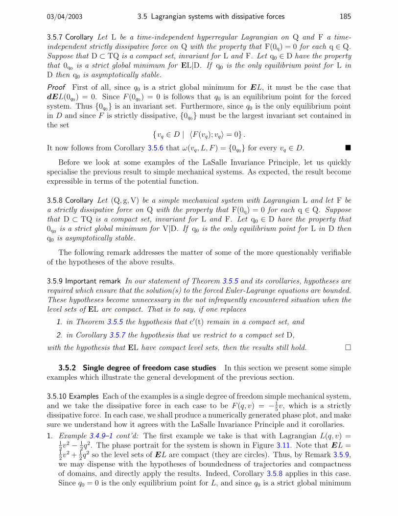
03/04/2003 3.5 Lagrangian systems with dissipative forces 185
3.5.7 Corollary Let L be a time-independent hyperregular Lagrangian on Q and F a time-independent strictly dissipative force on Q with the property that F(0q) = 0 for each q ∈ Q.Suppose that D ⊂ TQ is a compact set, invariant for L and F. Let q0 ∈ D have the propertythat 0q0 is a strict global minimum for EL|D. If q0 is the only equilibrium point for L inD then q0 is asymptotically stable.
Proof First of all, since q0 is a strict global minimum for EL, it must be the case thatdEL(0q0) = 0. Since F (0q0) = 0 is follows that q0 is an equilibrium point for the forcedsystem. Thus 0q0 is an invariant set. Furthermore, since q0 is the only equilibrium pointin D and since F is strictly dissipative, 0q0 must be the largest invariant set contained inthe set
vq ∈ D | 〈F (vq); vq〉 = 0 .
It now follows from Corollary 3.5.6 that ω(vq, L, F ) = 0q0 for every vq ∈ D.
Before we look at some examples of the LaSalle Invariance Principle, let us quicklyspecialise the previous result to simple mechanical systems. As expected, the result becomeexpressible in terms of the potential function.
3.5.8 Corollary Let (Q, g,V) be a simple mechanical system with Lagrangian L and let F bea strictly dissipative force on Q with the property that F(0q) = 0 for each q ∈ Q. Supposethat D ⊂ TQ is a compact set, invariant for L and F. Let q0 ∈ D have the property that0q0 is a strict global minimum for V|D. If q0 is the only equilibrium point for L in D thenq0 is asymptotically stable.
The following remark addresses the matter of some of the more questionably verifiableof the hypotheses of the above results.
3.5.9 Important remark In our statement of Theorem 3.5.5 and its corollaries, hypotheses arerequired which ensure that the solution(s) to the forced Euler-Lagrange equations are bounded.These hypotheses become unnecessary in the not infrequently encountered situation when thelevel sets of EL are compact. That is to say, if one replaces
1. in Theorem 3.5.5 the hypothesis that c′(t) remain in a compact set, and
2. in Corollary 3.5.7 the hypothesis that we restrict to a compact set D,
with the hypothesis that EL have compact level sets, then the results still hold.
3.5.2 Single degree of freedom case studies In this section we present some simpleexamples which illustrate the general development of the previous section.
3.5.10 Examples Each of the examples is a single degree of freedom simple mechanical system,and we take the dissipative force in each case to be F (q, v) = −1
5v, which is a strictly
dissipative force. In each case, we shall produce a numerically generated phase plot, and makesure we understand how it agrees with the LaSalle Invariance Principle and it corollaries.
1. Example 3.4.9–1 cont’d: The first example we take is that with Lagrangian L(q, v) =12v2 − 1
2q2. The phase portrait for the system is shown in Figure 3.11. Note that EL =
12v2 + 1
2q2 so the level sets of EL are compact (they are circles). Thus, by Remark 3.5.9,
we may dispense with the hypotheses of boundedness of trajectories and compactnessof domains, and directly apply the results. Indeed, Corollary 3.5.8 applies in this case.Since q0 = 0 is the only equilibrium point for L, and since q0 is a strict global minimum

186 3 Lagrangian dynamics 03/04/2003
-0.75 -0.5 -0.25 0 0.25 0.5 0.75 1
-0.75
-0.5
-0.25
0
0.25
0.5
0.75
1
PSfrag replacements
q(t)
qq(t)v(t)
v(t
)
vx(t)y(t)
V (q)
-1.5 -1 -0.5 0 0.5 1 1.5 2
-1.5
-1
-0.5
0
0.5
1
1.5
2
PSfrag replacements
q(t)
qq(t)v(t)
v(t
)
vx(t)y(t)
V (q)
-3 -2 -1 0 1 2 3-3
-2
-1
0
1
2
3
PSfrag replacements
q(t)
qq(t)v(t)
v(t
)
vx(t)y(t)
V (q)
Figure 3.11 Phase portraits for dissipative systems with La-grangians L(q, v) = 1
2v2− 12q2 (top left), L(q, v) = 1
2v2 + 12q2−
14q4 (top right), and L(q, v) = 1
2v2 + cos q (bottom). In eachcase the dissipative force is F (q, v) = −1
5v.
for V , Corollary 3.5.8 implies that q0 is an asymptotically stable equilibrium point. Thisis clearly seen from the phase portrait as well.
2. Example 3.4.10–1 cont’d: Next we take the Lagrangian L(q, v) = 12v2 + 1
2q2 − 1
4q4. The
phase portrait is shown in Figure 3.11. Note that the level sets of the energy are againcompact, so we need no special hypotheses concerning bounded trajectories or com-pact domains. Note that there are three equilibrium points, so we cannot apply Corol-lary 3.5.8. Let us apply Corollary 3.5.6. We have
vq ∈ TQ | 〈F (vq); vq〉 = 0 = (q, 0) | q ∈ R .
The maximal invariant set Ω contained in this set is then comprised of the three fixedpoints. Thus, in the notation of Corollary 3.5.6, Ω = (−1, 0) ∪ (0, 0 ∪ (1, 0). Itthen follows from Corollary 3.5.6 that for each (q, v) ∈ TQ, the positive limit set must be

03/04/2003 3.6 Rigid body dynamics 187
one of these three points. And indeed from Figure 3.11 we see that all initial conditionsend up in one of the fixed points. In fact, almost all trajectories end up in one of the twostable fixed points at (−1, 0) and (1, 0). The only initial conditions which end up at theunstable fixed point at (0, 0) are those which lie on the stable manifold for this point.
3. Example 3.4.10–2 cont’d: As our final example, we take L(q, v) = 12v2 + cos q. The
phase portrait is shown in Figure 3.11, and the discussion goes much as in the previousexample.
The mantra of the examples in this section seems to be that dissipation will make astable equilibrium point into an asymptotically stable equilibrium point. This is true forthe kinds of systems we have been looking at, but care must be taken when extending thisas a general principle. In [Lewis and Murray 1995] a mechanical system is investigated forwhich the introduction of dissipation causes instability of previously stable motions. Thisphenomenon is examined in a general setting by Bloch, Krishnaprasad, Marsden and Ratiu[1993]. See also Exercise E3.13.
3.6 Rigid body dynamics
While we spent a significant portion of Chapter 1 talking about rigid bodies, and howthey move in space, and in Section 2.8 we demonstrated that Euler’s equations for a rigidbody are equivalent to the Euler-Lagrange equations, we have yet to say anything about theactual solutions to the rigid body equations. Thus in this section we tackle this problem,describing these solutions in the absence of external forces.
The differential equations we concentrate on then are those for the body velocities aboutthe centre of mass. We make the assumption that the rigid motion undergone by the rigidbody is observed by a compatible observer. Thus, you will recall, the equations we look atare
R(t) = R(t)Ω(t)
r(t) = R(t)V (t)
Ic(Ω(t)) =(Ic(Ω(t))
)×Ω(t)
µ(B) V (t) = µ(B) V (t)×Ω(t),
(3.5)
where (R, r,Ω,V ) ∈ SO(3)× (R3)3. The meat of these equations is in the third equation
Ic(Ω(t)) =(Ic(Ω(t))
)×Ω(t). (3.6)
Indeed, once one has the solution t 7→ Ω(t) to this equation, the equation for the bodyvelocity V is then a time-dependent linear differential equation, as is the differential equationfor R. Finally, once one has t 7→ V (t) and t 7→ R(t), one may directly integrate to get r(t).However, the equation for Ω is nonlinear, and its solutions are quite interesting, so that iswhere we shall focus our attention.
3.6.1 Conservation laws and their implications It turns out that everything we needto know about equations (3.5) may be derived from the conservations laws these equationspossess. This is true even of the more difficult equation (3.6). The following result classifiesall the conserved quantities.
3.6.1 Theorem Let (B, µ) be a rigid body. For the equations (3.5), the following quantitiesare constant along solutions:

188 3 Lagrangian dynamics 03/04/2003
(i) the spatial linear momentum m(t) = µ(B)R(t)V(t);
(ii) the translational kinetic energy ET(t) = 12µ(B) ‖r(t)‖;
(iii) the rotational kinetic energy ER(t) = 12gcan(Ic(Ω(t)),Ω(t));
(iv) the length of the body angular momentum vector LR(t) = ‖Ic(Ω(t))‖.
Proof (i) We compute
m(t) = µ(B) R(t)V (t) + µ(B) R(t)V (t)
= µ(B) R(t)Ω(t)V (t) + µ(B) R(t)V (t)×Ω(t)
= 0.
(ii) Here we use the fact that m(t) = µ(B)r(t). From (i) we thus conclude that r(t) isconstant. From this the conclusion that ET (t) is constant immediately follows.
(iii) We compute
ER(t) =1
2gcan(Ic(Ω(t)),Ω(t)) +
1
2gcan(Ic(Ω(t)), Ω(t))
= gcan(Ic(Ω(t)),Ω(t)),
using the fact that Ic is symmetric with respect to gcan. Now we use (3.6) to give
ER(t) = gcan
((Ic(Ω(t)))×Ω(t),Ω(t)
)= gcan
(Ic(Ω(t)),Ω(t)×Ω(t)
)= 0,
where we have used the vector identity (1.19).(iv) From (iii) we know that if LR(0) = 0 then LR(t) = 0 for all t. Thus we may suppose
that LR(0) 6= 0. We compute
dL2R
dt= 2gcan
((Ic(Ω(t)), Ic(Ω(t))
)= 2gcan
((Ic(Ω(t)))×Ω(t), Ic(Ω(t))
)= − 2gcan
(Ω(t), (Ic(Ω(t)))× (Ic(Ω(t)))
)= 0.
But we also havedL2
R
dt= 2LR(t)LR(t). Since we are assuming that LR(0) 6= 0 it follows that
LR(0) = 0, and from this that LR(t) = LR(0) for all t, as desired.
Some of the statements of this theorem are unsurprising, but some are perhaps notobvious.
3.6.2 Remarks 1. That the spatial linear momentum is conserved should be in no way sur-prising. After all, in Section 1.6 we used this very fact to derive the equations (3.5)! Aconsequence of this conservation law is that the centre of mass of a rigid body in theabsence of forces moves at a uniform velocity.
2. That the total kinetic energy should be preserved is, of course, a consequence of conser-vation of energy for general Euler-Lagrange equations (cf. Proposition 2.5.7). It is notquite so obvious, perhaps, that the translational and rotational components should beindividually preserved.

03/04/2003 3.6 Rigid body dynamics 189
3. The most interesting conservation law is that for LR, the length of the body angularmomentum vector. It is this conservation law which will allow us to describe the solutionsof the equation (3.6). Its presence is an artifact of the conservation of spatial angularmomentum, and is reflective of similar statements in a more general setting, as presentedin Section 4.4 of [Abraham and Marsden 1978]. Interestingly, this phenomenon appearsin a different manner for a wide variety of physical problems. For example, Arnol’d [1966]uses a setting like this to provide an interpretation of “helicity” as a conservation law inthe flow of an inviscid incompressible fluid. Check
The statement 1 is of sufficient interest to merit its separate statement.
3.6.3 Corollary The centre of mass of a rigid moves at a constant velocity with respect to anobserver which is compatible with the rigid motion.
Let us now use the fact that ER and LR are constants of motion to obtain a descriptionof the solutions to (3.6).
3.6.4 Proposition Let (B, µ) be a rigid body and let I1, I2, I3 be the principal inertias withv1,v2,v3 the corresponding principal axes. We have the following four case, which classifyall possibilities up to permutation of the principal inertias.
(i) The principal inertias are strictly positive and not all equal: The solutions to (3.6) lieon the intersection of an ellipsoid
Ω ∈ R3∣∣ ‖I(Ω)‖ = C1
and an ellipsoid
Ω ∈ R3∣∣ gcan(Ic(Ω),Ω) = C2
for some C1,C2 > 0.
(ii) 0 = I1 < I2 = I3: The solutions to (3.6) are all of the form t 7→ Ω0 + ω(t)v1 whereΩ0 ∈ spanR v2,v3 and where t 7→ ω(t) ∈ R is arbitrary.
(iii) 0 = I1 = I2 = I3: Any curve t 7→ Ω(t) is a solution to (3.6).
Proof (i) This follows directly from parts (iii) and (iv) of Theorem 3.6.1. In this case sinceIc is invertible, the set
Ω ∈ R3∣∣ ‖Ic(Ω)‖ = C1
and the set
Ω ∈ R3∣∣ gcan(Ic(Ω),Ω) = C2
are indeed ellipsoids.
(ii) Recall from Proposition 1.5.6(ii) that a single zero principal inertia implies that theother two principal inertias must be equal. If (x1, x2, x3) denotes coordinates for R3 withrespect to the principal axes, then the condition (iii) of Theorem 3.6.1 reads
I((x2)2 + (x3)2
)= constant,
and the condition (iv) reads
I2((x2)2 + (x3)2
)= constant,
where I = I2 = I3. Thus one cannot make a conclusive statement regarding the solu-tions of (3.6) from the conservation laws alone. However, substituting the inertias directly

190 3 Lagrangian dynamics 03/04/2003
into (3.6) gives the equations x1 = 0, x2 = 0, and 0 = 0. Thus x1 and x2 are constant, andx3 is arbitrary, just as stated in the proposition.
(iii) In this case we note that (3.6) is simply the identity 0 = 0. Thus any curve in R3
will indeed be a solution.
The only really interesting case is part (i) of the proposition. We shall give this moreattention shortly, but for now let us make some general remarks about the other cases.
3.6.5 Remarks 1. The case (i) covers the most interesting cases, and we shall investigate thisin detail in the next section.
2. The case (ii) corresponds, as shown in the proof of Proposition 1.5.6(ii), to the case wherethe support of µ is contained in a line. The motion described in part (ii) of the aboveproposition simply says that the angular velocity about this line is irrelevant since thebody has no inertia to resist this angular velocity. The equations are degenerate becausethree angular velocities are one too many in this case. One should properly describe thesystem with a two-dimensional set of angular velocities.
3. The most degenerate case, case (iii), corresponds to a rigid body which is a point mass.In this case, the remarks from the previous case apply to all angular velocities since thebody has no angular inertia. Therefore the three angular velocities have no meaning forthe motion of the body in this case.
3.6.2 The evolution of body angular momentum Let us now proceed to discuss inmore detail the case (i) of Proposition 3.6.4. Since the length of the body angular momentumis constant along solutions of (3.6), it is convenient to change coordinates from body angularvelocity to body angular momentum, since in momentum space, all solutions lie on spheresof constant radius. The differential equation describing body angular momentum when Ic isinvertible is
M(t) = M(t)×(I−1c (M(t))
). (3.7)
It is this equation we proceed to analyse. First we note that the conservation laws for ER
and LR in Theorem 3.6.1 when expressed in terms of body angular momentum imply thatER(t) = 1
2gcan(Ic(M(t)),M(t)) and LR(t) = ‖M(t)‖ are constant along solutions of (3.7).
The sets of constant value for LR are, of course, spheres, and the sets of constant value forER are ellipsoids. The solutions must therefore lie on the intersection of some such sphereand some such ellipsoid.
Let us proceed to formally analyse (3.7). First let us find its fixed points.
3.6.6 Proposition Let (B, µ) be a rigid body with principal inertias I1, I2, I3 arranged so that0 < I1 ≤ I2 ≤ I3, and let v1,v2,v3 be the corresponding principal axes. If F (B, µ) ⊂ R3
denotes the fixed points of equation (3.7) which occur on the sphere of radius R, then
(i) when I1 < I2 < I3 we have
F (B, µ) = ±Rv1 ∪ ±Rv2 ∪ ±Rv3;
(ii) when I1 = I2 < I3 we have
F (B, µ) =
a1v1 + a2v2 | a21 + a2
2 = R2∪ ±Rv3;

03/04/2003 3.6 Rigid body dynamics 191
(iii) when I1 < I2 = I3 we have
F (B, µ) = ±Rv1 ∪
a2v2 + a3v3 | a22 + a2
3 = R2
;
(iv) when I1 = I2 = I3 we have
F (B, µ) =
a1v1 + a2v2 + a3v3 | a21 + a2
2 + a23 = R2
.
Proof From (3.7) we see that M ∈ R3 is a fixed point if and only if M and I−1c (M) are
collinear. Thus M is a fixed point if and only if it is an eigenvector of I−1c if and only if it is
an eigenvector of Ic. The result now follows by our discussion in the course of the proof ofProposition 1.5.8 about the eigenvectors of Ic when it has equal eigenvalues.
Now let us determine the stability of the various fixed points by linearising, and com-puting the eigenvalues of the linearised system. Suppose that M 0 is a fixed point for (3.7).Then, as we saw in the proof of Proposition 3.6.6, M 0 must be an eigenvector for I−1
c , so wemust have Ic(M 0) = I−1
a M 0 for some principal inertia Ia, a ∈ 1, 2, 3 (here we use the factthat the eigenvalues of an invertible matrix are the inverse of the eigenvalues of the matrix).Linearising (3.7) about such a fixed point gives the linearised equations
ξ(t) = ξ(t)×(I−1c (M 0)
)+ M 0 ×
(I−1c (ξ(t))
)= M 0 ×
(I−1c (ξ(t))− I−1
a ξ(t)).
Now let us write ξ(t) in a principal basis we
ξ(t) = ξ1(t)v1 + ξ2(t)v2 + ξ3(t)v3,
and let us suppose that we have permuted the principal inertias so that a = 3. Then wehave suppose that M 0 = M0v3 for some M0 ∈ R. Since I−1
c (v3) = I−13 v3, we have ξ3(t) = 0.
We then compute
ξ1(t) = M0(I−12 − I−1
3 )ξ2(t)
ξ2(t) = M0(I−13 − I−1
1 )ξ1(t).
Thus the eigenvalues for the linearised system are 0 (which is an eigenvalue with eigenvectorv3) and the eigenvalues of the matrix
M0
[0 I−1
2 − I−13
I−13 − I−1
1 0
]. (3.8)
These latter eigenvalues are the roots of the polynomial
λ2 +M20 (I−1
2 − I−13 )(I−1
1 − I−13 ). (3.9)
Note that the automatic zero eigenvalue is not a surprise since its eigenvector is orthogonalto the sphere of constant length for body angular momentum. It is the very preservationof this sphere which makes this eigenvalue zero. The other two eigenvalues are, therefore,the ones which interest us as they are in directions tangent to the body momentum sphere.From (3.9) we may immediately deduce the following result.

192 3 Lagrangian dynamics 03/04/2003
3.6.7 Proposition Let (B, µ) be a rigid body with principal inertias I1, I2, I3, and supposewithout loss of generality that I1 ≤ I2. Let M0 be a fixed point of (3.7) corresponding tothe principal inertia I3 (i.e., M0 is an eigenvalue of I−1
c with eigenvalue I−13 ). Then 0 is an
eigenvalue for the linearisation of (3.7) about M0, and the other eigenvalues are given asfollows:
(i) I1 < I3 < I2: eigenvalues are ±M0
√(I−1
3 − I−12 )(I−1
1 − I−13 );
(ii) I3 < I1 < I2: eigenvalues are ±iM0
√(I−1
3 − I−12 )(I−1
3 − I−11 );
(iii) I1 < I2 < I3: eigenvalues are ±iM0
√(I−1
2 − I−13 )(I−1
1 − I−13 );
(iv) I1 = I2 < I3: eigenvalues are ±iM0
√(I−1
2 − I−13 )(I−1
1 − I−13 );
(v) I3 < I1 = I2: eigenvalues are ±iM0
√(I−1
3 − I−12 )(I−1
3 − I−11 );
(vi) I1 < I2 = I3: all eigenvalues are zero;
(vii) I1 = I3 < I2: all eigenvalues are zero;
(viii) I1 = I2 = I3: all eigenvalues are zero.
It is now easy to turn this into the following result concerning stability of the linearisationof (3.7) about fixed points.
3.6.8 Corollary Let (B, µ) be a rigid body. We have the following cases.
(i) If the principal inertias of B are distinct, then
(a) the linearisation for rotations about the intermediate principal axis are unstableand
(b) the linearisation for rotations about the largest and the smallest principal axes arestable.
(ii) If there are two equal principal inertias, then the linearisation about any of the fixedpoints is unstable.
(iii) If all principal inertias are equal, then the linearisation is stable.
Proof The only thing that is in doubt are the cases where all the eigenvalues are zero.For these cases, we need to ensure that there are 2 linearly independent eigenvectors forthe matrix (3.8). However, in all such cases, one verifies that the matrix (3.8) has rank 1when only two eigenvalues are equal; this means that the linearisation is unstable. When alleigenvalues are equal, then the matrix (3.8) is identically zero, so it indeed has two linearlyindependent eigenvectors.
This then completes the linear stability analysis of the fixed points for (3.7). When thelinearisation is unstable, this it is so by virtue of there being a positive real eigenvalue, sothe Unstable Manifold Theorem ensures instability of the full equations at such fixed points.However, in all of the cases when the linearisation is stable, it is stable with all eigenvalues onthe imaginary axis, so one cannot conclude stability of the full equations from the linearisedequations (as seems to be the way with mechanical systems). However, since the solutionsrestricted to the spheres on must also lie on the ellipsoids of constant energy, one may use thisto help determine the character of the full nonlinear equations. Indeed, if you are good atimagining such things, imagine fixing a sphere of some radius, and starting with an ellipsoidwhich sits in the interior of the sphere. Now gradually grow the ellipsoid. Eventually itwill touch the sphere, and as the ellipsoid grows further, the points or lines of intersectionwill determine the solutions of (3.7). By growing the ellipsoid in this manner one obtains

03/04/2003 3.6 Rigid body dynamics 193
Figure 3.12 Solutions for equation (3.7) when I1 = I2 < I3 (topleft), when I1 < I2 = I3 (top right), and when I1 < I2 < I3
(bottom)
all solutions as each point on the sphere will intersect some ellipsoid. In Figure 3.12 isdepicted a numerically generated set of solution curves for (3.7) in the various cases. Notethat in these pictures we always assume I1 ≤ I2 ≤ I3, in order to reduce the number ofcases we need to plot. This is in contrast with Proposition 3.6.7 and Corollary 3.6.8 wherethe principal inertias were considered arranged so that we are interested in the fixed pointscorresponding to the third principal inertia. Also, in Figure 3.12 we do not include the casewhere I1 = I2 = I3. In this case, all points are fixed points, and so stable.
Let us summarise the conclusions one may derive from Figure 3.12.
3.6.9 Proposition Let (B, µ) be a rigid body with principal inertias I1, I2, I3, and supposewithout loss of generality that I1 ≤ I2. Let M0 be a fixed point of (3.7) corresponding to theprincipal inertia I3 (i.e., M0 is an eigenvalue of I−1
c with eigenvalue I−13 ). The stability of
M0 is given as follows:
(i) I1 < I3 < I2: unstable;
(ii) I3 < I1 < I2: stable;
(iii) I1 < I2 < I3: stable;
(iv) I1 = I2 < I3: stable;
(v) I3 < I1 = I2: stable;

194 3 Lagrangian dynamics 03/04/2003
(vi) I1 < I2 = I3: unstable;
(vii) I1 = I3 < I2: unstable;
(viii) I1 = I2 = I3: stable.
Fixed points are never asymptotically stable.
3.6.3 Poinsot’s description of a rigid body motion Louis Poinsot (1777–1859) de-vised a clever way to visualise the solutions to (3.7). Poinsot’s description tells us how thebody itself moves in space, as opposed to Euler’s equation which tells us how the angularmomentum vector looks in a frame moving with the body. In this section, as in our previousdiscussion of rigid body dynamics, we fix a centre of mass observer adapted to the rigidmotion, and a coordinate system adapted to this observer. The description of Poinsot relieson the inertial ellipsoid discussed in Section 1.5.3. With our conventions for the observerand the coordinate system, the inertial ellipsoid becomes the subset of R3 given by
E(B) =Ω ∈ R3
∣∣ gcan(Ic(Ω),Ω) = 1.
We think of the inertial ellipsoid as being attached to the body so that the axes of theellipsoid align with the corresponding principal axes of the body. As the body moves inspace, so too will the inertial ellipsoid move in space. It is this motion of the inertialellipsoid which Poinsot describes. For simplicity, we assume that the centre of mass of thebody is stationary, i.e., that the spatial linear momentum, which is conserved, is zero.
The following result gives Poinsot’s description. You will recall that spatial angularmomentum is constant along natural motions of a rigid body; indeed, we used this veryproperty to derive the governing equations.
3.6.10 Theorem (Poinsot’s description of rigid body motion) Let (B, µ) be a rigid body andlet the equations
R(t) = R−1(t)Ω(t)
Ic(Ω(t)) =(Ic(Ω(t))
)×Ω(t)
describe the angular motion of the body, and suppose that the centre of mass of the body isstationary. Also suppose that none of the principal inertias of the body are zero. The solutiont 7→ R(t) has the property that the family of ellipsoids t 7→ R(t)(E(B)) rolls without slippingon a stationary plane P orthogonal to the (constant) spatial angular momentum vector `.The plane P is called the invariable plane.
Proof Suppose that the rigid motion has rotational kinetic energy e so that all motion takesplace on the body angular momentum sphere of radius
√2e. We work first in a body frame
where the inertial ellipsoid is stationary. We define a plane Pt which is tangent to E(B) atthe point Ω(t). At the point Ω(t) ∈ E(B) we determine the that the normal to E(B) isgiven by
grad(gcan(Ic(Ω),Ω)
)|Ω=Ω(t) = 2Ic(Ω(t)) = 2L(t).
A translated plane Pt orthogonal to this normal vector should satisfy
Pt =
x ∈ R3∣∣ gcan
(x, 2Ic(Ω(t))
)= C
(3.10)
for some C ∈ R. However, since the point Ω(t) must satisfy the constraint of conservationof rotational energy, we must have
gcan
(Ω(t), 2Ic(Ω(t))
)= 2e.

03/04/2003 3.7 Geodesic motion 195
Therefore, by the definition of the inertial ellipsoid, the point Ω(t)/√
2e must lie in E(B).Indeed we have
gcan
(I(Ω(t)/
√2e),Ω(t)/
√2e)
=1
2egcan
(I(Ω(t)),Ω(t)
)= 1.
Therefore (3.10) defines a plane Pt tangent to the inertial ellipsoid at time t provided thatwe take C =
√2e. Thus we have
Pt =x ∈ R3
∣∣ gcan(x,L(t)) =√
2e.
We now move to a spatial frame. Fix the same time t and define the ellipsoid Et(B) =R(t)(E(B)). The body velocity Ω(t) gets mapped to the spatial velocity ω(t) = R(t)(Ω(t)).The plane Pt is mapped to the plane P = R(t)(Pt) which is therefore tangent to Et(B) atthe point ω(t). Therefore P satisfies
P =y ∈ R3
∣∣ gcan(L(t),R−1(t)(y)) =√
2e
=y ∈ R3
∣∣ gcan(R(t)L(t), (y)) =√
2e
=y ∈ R3
∣∣ gcan(`(t), (y)) =√
2e.
Now since `(t) is constant, this shows that the plane P is independent of t. Thus we haveshown that the ellipsoids Et(B) do indeed roll along the plane P . It remains to be shownthat they roll without slipping.
This latter fact will follow if we note that the point of contact of Et(B) with the planeP lies at a point ω(t)/
√2e which is on the line of instantaneous rotation of the body. Since
all points along this line have zero instantaneous spatial velocity, our result follows.
A picture corresponding to Poinsot’s description is given in Figure 3.13. We referto [Arnol’d 1989] for a few applications of Poinsot’s description of rigid body motion todetermining the character of this motion. Also see Exercise E3.7.
3.7 Geodesic motion
In our analysis of the stability of equilibrium points Section 3.2—and particularly in ouranalysis of simple mechanical systems in Section 3.3.1—we paid little attention to the casewhere KL(q0) and CL(q0) are both zero. However, for the class of simple mechanical systemswith no potential force, this will always be the case, cf. Proposition 3.3.7. Therefore, noneof our preceding stability analysis has much relevance for this important class of systems.In this section we will study such systems and say what little we can about them; they area very complicated class of system, interestingly made more complicated in some ways bythe absence of a potential function.
3.7.1 Basic facts about geodesic motion In Section 2.4.4 we showed how the equa-tions of motion for a simple mechanical system (Q, g, 0) with a zero potential function aregeodesics of a particular affine connection—the Levi-Civita connection—which is associatedwith the Riemannian metric g. However, it is of no particular advantage to specialise tothe case of the Levi-Civita connection, so in this section we consider a general affine con-nection ∇ on Q. Recall that in a coordinate chart one defines the Christoffel symbols Γi
jk,

196 3 Lagrangian dynamics 03/04/2003
PSfrag replacements
q(t)q
q(t)v(t)v(t)
vx(t)y(t)
V (q)
Figure 3.13 Poinsot’s description of the motion of a rigid body
i, j, k = 1, . . . , n, as in (2.11). Geodesics are then curves on Q which in coordinates satisfythe second-order differential equation
qi + Γijkq
j qk = 0, i = 1, . . . , n.
From this equation, we immediately have the following result. The result uses factsabout geodesic normal coordinates which we do not know about (see [Kobayashi and Nomizu1963]).
3.7.1 Proposition For a simple mechanical system (Q, g, 0) with zero potential function, allpoints in Q are equilibrium points, none are linearly stable, and none are stable for thenonlinear system.
Proof That all points in Q are equilibrium points follows from Proposition 3.3.6. FromProposition 3.3.7 we see that at every equilibrium point, i.e., every point q0 ∈ Q, we have
AL(q0) =
[0 idTq0Q
0 0
].
Thus all eigenvalues of AL(q0) are zero, but dim(ker(AL(q0))) = n so the fixed points arelinearly unstable since the geometric and algebraic multiplicities of the eigenvalues on theimaginary axis are not the same. Finally, let us show that the equilibria are not stable forthe full system. This follows from the fact that about each point q0 ∈ Q we may find a“normal” set of coordinates (q1, . . . , qn) with the property that any geodesic t 7→ c(t) withinitial condition c′(0) = vq0 ∈ Tq0Q has the form t 7→ vt for some v ∈ Rn. Such a curve

03/04/2003 3.7 Geodesic motion 197
will leave any sufficiently small neighbourhood of q0 in finite time, implying the equilibriumpoint is unstable.
Clearly such systems must be of interest for things other than their equilibria, sinceequilibria are abundant and all unstable. The following result gives a distinctive propertyfor solutions of the geodesic equations. Note that the result is not generally true for solutionsof the Euler-Lagrange equations for arbitrary Lagrangians.
3.7.2 Proposition Let ∇ be an affine connection on a configuration space Q. Let c : [0,T] →Q be a curve and for λ > 0 define a new curve cλ : [0, T
λ] → Q by cλ(t) = c(λt). Then, if c
is a geodesic, so is cλ.
Proof In coordinates represent c by t 7→ (q1(t), . . . , qn(t)) so that we have
d2qi
dt2+ Γi
jk
dqj
dt
dqk
dt= 0, i = 1, . . . , n.
Now define τ = λt and compute
d2qi
dτ 2+ Γi
jk
dqj
dτ
dqk
dτ= λ2
(d2qi
dt2+ Γi
jk
dqj
dt
dqk
dt
), i = 1, . . . , n,
which gives the result.
Note that with the notation of the preceding result we have c′λ(0) = λc′(0). The idea ofthe result is therefore that if one scales the initial velocity of a given geodesic, the resultinggeodesic will follow the same path as the original, but will simply do so more quickly ormore slowly, depending on whether λ > 1 or λ < 1.
3.7.2 The Jacobi metric It turns out that even when the potential function isnonzero, one may still describe the motion of a simple mechanical system as geodesic motion.That this is possible is a discovery of Carl Gustav Jacob Jacobi (1804–1851). The principalobservation is that since kinetic energy is always nonnegative, if a solution t 7→ c(t) has totalenergy e, then the potential energy should satisfy V (c(t)) ≤ e. For this reason, solutions oftotal energy e will evolve in the subset
Qe = q ∈ Q | V (q) ≤ e .
Let us also denoteQe = q ∈ Q | V (q) < e .
Note that on Qe the function q 7→ e−V (q) is strictly positive. Therefore, given a Riemannianmetric g on Q, at points q ∈ Qe, ge(q) = (e − V (q))g(q) defines an inner product on TqQ.Therefore, this defines a Riemannian metric ge on Qe called the Jacobi metric.
We now state the relationship between the Riemannian metric ge on Qe and solutions ofthe Euler-Lagrange equations.
3.7.3 Theorem Let (Q, g,V) be a simple mechanical system with Lagrangian L and let e ∈ Rhave the property that Qe 6= ∅. If vq ∈ EL−1(e), then the solution to the Euler-Lagrangeequations with initial condition vq agrees up to reparameterisation with the geodesic of theJacobi metric with initial velocity vq.
198 3 Lagrangian dynamics 03/04/2003
Proof Lete
∇ be the Levi-Civita connection associated with the Riemannian metric ge. Webegin with a computational lemma.
1 Lemma Let e2ρ = (e− V), so defining ρ. Then we have
e
∇XY =g
∇XY + 〈dρ; X〉Y + 〈dρ; Y〉X− g(X,Y) grad ρ.
Proof In coordinates we have
(e
∇XY )i =∂Y i
∂qjXj +
e
ΓijkX
jY k, i = 1, . . . , n,
wheree
Γ are the Christoffel symbols fore
∇. The result will then follow if we can show that
e
Γijk =
g
Γijk +
∂ρ
∂q`X`Y i +
∂ρ
∂q`Y `X i − g`mX
`Y mgir ∂ρ
∂qr, i, j, k = 1, . . . , n. (3.11)
By definition of the Levi-Civita Christoffel symbols we have
e
Γijk =
1
2(ge)
i`(∂(ge)`j
∂qk+∂(ge)`k
∂qj− ∂(ge)jk
∂q`
), i, j, k = 1, . . . , n. (3.12)
However, since (ge)ij = e2ρgij, i, j = 1, . . . , n, we directly compute
∂(ge)ij
∂qk= 2e2ρ ∂ρ
∂qkg`j + e2ρ∂gij
∂qk, i, j, k = 1, . . . , n. (3.13)
Plugging (3.13) into (3.12) gives (3.11) after some manipulation. H
Now let us proceed with the remainder of the proof. Fix a solution c to the Euler-Lagrange equations for L. We compute
d(e2ρ) = −dV =⇒ 2e2ρdρ = −dV =⇒ 2(e− V )dρ = −dV. (3.14)
By conservation of energy we also have
g(c′(t), c′(t)) = 2(e− V ), (3.15)
which using (3.14) givesg(c′(t), c′(t)) grad ρ = − gradV. (3.16)
Since c is a solution to the Euler-Lagrange equations we have
g
∇c′(t)c′(t) = − gradV (c(t)).
Using Lemma 1 and (3.16) we obtain
e
∇c′(t)c′(t) =
g
∇c′(t)c′(t) + 2 〈dρ; c′(t)〉 c′(t) + g(c′(t), c′(t)) grad ρ
= − gradV (c(t)) + 2 〈dρ; c′(t)〉 c′(t) + g(c′(t), c′(t)) grad ρ
= 2 〈dρ; c′(t)〉 c′(t).

03/04/2003 3.8 The dynamics of constrained systems 199
Now reparameterise c with the time parameter τ defined so that dτdt
= (e − V ). We thenhave
dc
dτ=
dt
dτc′(t) =
1
e− Vc′(t) = e−2ρc′(t).
We then compute
e
∇ dcdτ
dc
dτ=
e
∇e−2ρc′(t)(e−2ρc′(t))
= e−2ρe
∇c′(t)(e−2ρc′(t))
= e−4ρe
∇c′(t)c′(t) + e−2ρ(L c′(t)e
−2ρ)c′(t)
= e−4ρ( e
∇c′(t)c′(t)− 〈dρ; c′(t)〉 c′(t)
)= 0.
In deriving this formula, we have used the defining properties of an affine connection given in
Definition 2.4.7. Note that we have shown that c is a geodesic ofe
∇ provided we parameteriseit with the time parameter τ .
Ong [1975] provides a nice discussion of various aspects of dynamics of simple mechanicalsystems using the Jacobi metric. The substance of the above proof comes from Ong. Onecould, I suppose, give an application of Theorem 3.7.3, but it would not be an exercise whichwould shed any more light on the subject. We should really think of Theorem 3.7.3 as aninteresting theoretical tidbit, although it may have some useful dynamical consequences insome examples.
3.8 The dynamics of constrained systems
Let us complete our incomplete discussion of Lagrangian dynamics with a few wordsabout the dynamics of constrained systems. Owing to the fact that the body of workconcerning the dynamics of constrained systems is minimal, our discussion only touchesupon a few basic questions. Some issues are dealt with more thoroughly by Neımark andFufaev [1972], but even there the authors remark on the lack of a consistent approach to thesubject of dynamics for systems with constraints.
3.8.1 Existence of solutions for constrained systems In Section 3.1 we saw thathyperregularity of L was sufficient to guarantee that the solutions to the Euler-Lagrangeequations are determined by an ordinary differential equation, and so subject to the existenceand uniqueness theory of ordinary differential equations. For constrained systems, mattersare not so simple, as is illustrated by a simple example.
3.8.1 Example We consider Q = R2 with the time-independent hyperregular LagrangianL(x, y, vx, vy) = 1
2(v2
x − v2y). As a constraint we take the linear constraint
C(x,y) = (vx, vy) | vx + vy = 0 .
The constraints are annihilated by the single one-form α = dx−dy. Thus we have a perfectlywell-behaved Lagrangian and a perfectly well-behaved constraint. However, when we putthem together, we get the constrained equations of motion
x = 1, −y = −1.

200 3 Lagrangian dynamics 03/04/2003
Therefore we must have x = y. But the constraint equations give us x = −y, so we musthave x = y = 0. This, however, is an immediate contradiction of the equations of motion.
It is not immediately obvious what is the problem with the previous example. However,after some thought, one sees that the difficulty lies in the fact that the quadratic form withmatrix ∂2L
∂vi∂vj is degenerate on the subspace of virtual displacements. More specifically, thequadratic form represented by the matrix[
1 00 −1
]is identically zero when evaluated on vectors in spanR (1,−1). Let us convince ourselvesthat this is indeed a source of problems by looking at the same constraint, but with aLagrangian for which the quadratic form with matrix ∂2L
∂vi∂vj is nondegenerate on the subspaceof virtual displacements.
3.8.2 Example (Example 3.8.1 cont’d) We maintain the constraint from Example 3.8.1 butconsider a different Lagrangian. We take L(x, y, vx, vy) = 1
2(v2
x + v2y). In this case the
equations of motion readx = 1, y = −1,
from which we derive x = −y. These equations are now compatible with the constraints,and one can verify directly that any curve of the form
x(t) = x(0) + vt, y(t) = y(0)− vt
will satisfy the constraints for any v ∈ R. Note that this version of our example simplymodels a particle of unit mass constrained (by an holonomic constraint) to move along linesin R2 with slope −1.
Let us now reveal that the above example generalises in a natural manner.
3.8.3 Theorem Let L be a hyperregular Lagrangian on Q with C a constraint and F a force. Iffor each vq ∈ TQ the quadratic form with components ∂2L
∂vi∂vj , i, j = 1, . . . , n, is nondegenerateon the subspace `(Cq) ⊂ TqQ, then the solutions to the constrained Lagrangian system(L,F,C) satisfy a second-order differential equation.
Proof We work in a set of coordinates (q1, . . . , qn). Let α1, . . . , αn−r be a basis for ann(`(C))in these coordinates, and let η be a vector field on Q with the property that Cq = `(Cq)+η(q).The constrained equations of motion are then
∂2L
∂vi∂vjqj +
∂2L
∂vi∂qjqj +
∂2L
∂vi∂t− ∂L
∂qi= Fi + λaα
ai , i = 1, . . . , n
αai q
i = αai η
i, a = 1, . . . , n− r.
Differentiating the second equation with respect to time gives
αai q
i +∂αa
i
∂qjqiqj =
∂αai
∂qjηiqj + αa
i
∂ηi
∂qjqj, a = 1, . . . , n− r. (3.17)
Since L is hyperregular we may solve the first of the equations of motion for qi:
qi = Ai`( ∂L∂q`
− ∂2L
∂v`∂qjqj − ∂2L
∂v`∂t+ F` + λaα
a`
), i = 1, . . . , n, (3.18)

03/04/2003 3.8 The dynamics of constrained systems 201
where Ai`, i, ` = 1, . . . , n, are defined by
Ai` ∂2L
∂v`∂vj= δi
j, i, j = 1, . . . , n.
Substituting (3.18) into (3.17) and simplifying gives
αaiA
i`αb`λb =
∂αai
∂qjηiqj + αa
i
∂ηi
∂qjqj − ∂αa
i
∂qjqiqj−
αaiA
i`( ∂L∂q`
− ∂2L
∂v`∂qjqj − ∂2L
∂v`∂t+ F`
), a = 1, . . . , n− r. (3.19)
Now we use a lemma to complete the final step.
1 Lemma The (n − r) × (n − r) matrix with components αai A
i`αb` , a, b = 1, . . . , n − r, is
invertible.
Proof Suppose that we have β1, . . . , βn−r so that
αaiA
i`αb`βb = 0, a = 1, . . . , n− r.
This would imply that Ai`αb`βb, i = 1, . . . , n, are the components of the zero vector field in
`(C) since α1, . . . , αn−r form a basis for ann(`(C)). Since the quadratic form with matrix∂2L
∂vi∂vj , i, j = 1, . . . , n, is nondegenerate on `(C), we have
Ai`αb`βb = 0, i = 1, . . . , n
⇐⇒ ∂2L
∂vi∂vjAi`αb
`βb = αbjβb = 0, i = j, . . . , n.
Since the one-forms α1, . . . , αn−r are linearly independent, the result now follows. H
Using the lemma we may use (3.19) to solve for the Lagrange multipliers. Now we plugthese Lagrange multipliers back into (3.18), and the result is a set of second-order differentialequations, as desired.
3.8.4 Remarks 1. Of course, the value of the theorem is that it gives an existence and unique-ness result for constrained systems. Constrained systems are capable of a great deal ofexotic behaviour, so it is consoling to have some not unreasonable conditions whichguarantee that solutions exist and are unique.
2. We make use of “the quadratic form whose matrix is ∂2L∂vi∂vj , i, j = 1, . . . , n.” Well,
this is an actual quadratic form, and we actually demonstrated this in the proof ofProposition 3.2.10. If you look through the proof, you will see that when we demonstratedthat ML(q0) was independent of choice of coordinates, we never used the fact that weevaluated the quantities ∂2L
∂vi∂vj , i, j = 1, . . . , n, at zero velocity. This quadratic form isactually a quite useful object. Of course, for simple mechanical systems, it is simply theRiemannian metric.
3. Speaking of Riemannian metrics, note that the hypotheses of the theorem are satisfiedautomatically if L is the Lagrangian for a simple mechanical system (see Corollary 3.8.5below).
The upshot of Remark 3 is worth recording on its own.
202 3 Lagrangian dynamics 03/04/2003
3.8.5 Corollary If (Q, g,V) is a simple mechanical system with Lagrangian L, C is a con-straint on Q, and F is a force on Q, then whenever vq ∈ C is an initial condition satisfyingthe constraints, there exists a solution to the constrained system (L,F,C) with initial condi-tion vq. Furthermore, any two such solutions will agree on the intersection of their domains.
3.8.2 Some general observations In this section let us give answers to a few questionsof the form, “What aspects of dynamics for unconstrained Lagrangian systems carry overto constrained systems?” In particular, we concentrate on two questions, one concerningconservation of energy, and the other concerning the nature of the stability of equilibriumpoints.
Let us first consider the situation concerning conservation of energy.
3.8.6 Proposition Let L be a time-dependent Lagrangian on Q and C a constraint on Q.Suppose that t 7→ c(t) is a solution to the constrained Lagrangian system (L, 0,C) witht 7→ α(t) ∈ ann(`(Cc(t))) the corresponding constraint force. If EL denotes the energy of thesystem then we have
d
dtEL(t, c′(t)) = 〈α(t); c′(t)〉 .
In particular, if the constraint C is linear, then energy is conserved.
Proof We work in coordinates (q1, . . . , qn) with α1, . . . , αn−r a local basis for ann(`(C)).We also define a vector field η on Q so that Cq = `(Cq) + η(q). Recall that the equations ofmotion are then
d
dt
( ∂L∂vi
)− ∂L
∂qi= λaα
ai , i = 1, . . . , n
αai q
i = αai η
i, a = 1, . . . , n− r.
Following the computations of Proposition 2.5.7 we determine from the first of these equa-tions that
d
dtEL(t, c′(t)) = 〈α(t); c′(t)〉 ,
which is the first assertion of the proposition. The second assertion follows from the secondof the equations of motion since if C is linear we may take η = 0.
Now let us consider the matter of stability of equilibrium points. We have seen inSection 3.2 that it is not possible for an equilibrium point of an unconstrained system tobe asymptotically stable. However, this is not the case for systems with constraints, and solet us give an example of a constrained system with an asymptotically stable equilibriumpoint.
3.8.7 Example Finish this
3.8.3 Constrained simple mechanical systems In this section we address the natureof the equations which govern the dynamics of simple mechanical systems with constraints.The observation we make in this section seems to have originated with Synge [1928].
We consider a simple mechanical system (Q, g, 0) with no potential energy, and a linearconstraint C. The constructions we make are readily modified to include the potential

03/04/2003 3.8 The dynamics of constrained systems 203
function and to include constraints which are not necessarily linear. However, the clutter ofthis extra generality serves only to obscure the basic idea we illustrate.
Recall that in Section 2.6.4 we had introduced the g-orthogonal projection PC : TQ→ TQonto the orthogonal complement of the constraint distribution. Using this projection, inProposition 2.6.14 we had shown that solutions to the constrained system satisfy
g
∇c′(t)c′(t) = λ(t)
PC(c′(t)) = 0(3.20)
for some vector field t 7→ λ(t) ∈ C⊥c(t) along c taking its values in the subspaces orthogonal to
C. We wish to examine these equations, and eliminate the Lagrange multipliers in a cleverway.
Our construction requires that we be able to differentiate the projection PC in the correct
fashion. To this end, for a vector field X on Q, let us define a mapg
∇XPC : TQ → TQ as
follows: for any vector field Y on Q we requireg
∇XPC to satisfy
(g
∇XPC)(Y ) =g
∇X(PC(Y ))− PC(g
∇XY ).
In this manner we are able to defineg
∇XPC using our knowledge of how to defineg
∇ on vector
fields. Using this definition ofg
∇XPC we may show that in coordinates we have
(g
∇XPC)ij =
∂P ij
∂qkXk +
g
ΓiklP
ljX
k −g
ΓlkjP
ilX
k, i, j = 1, . . . , n, (3.21)
where P ij , i, j = 1, . . . , n, are the components of PC, and so are defined by
PC
( ∂
∂qj
)= P i
j
∂
∂qi, j = 1, . . . , n.
The expression (3.21) can be troublesome to compute in practice, much as PC can be abother to calculate. However, the utility of what we do in this section lies in its theoreticalcontent.
Let us see how to computeg
∇XPC in an example for which we have already computedPC.
3.8.8 Example (Example 2.6.1 cont’d) We carry on looking at the rolling disk example whereQ = R2 × T2, and we use coordinates (x, y, θ, φ). The constraints are defined by
x = r cos θφ, y = r sin θφ.
In Example 2.6.13 we determined that the components P ij , i, j = 1, . . . , 4, for the projection
PC are given by
1
mr2 + J
J +mr2 sin2 θ −mr2 sin θ cos θ 0 −rJ cos θ−mr2 sin θ cos θ J +mr2 cos2 θ 0 −rJ sin θ
0 0 0 0−mr cos θ −mr sin θ 0 mr2
.In Example 2.6.11 we saw that the Christoffel symbols are all identically zero for the Rie-
mannian metric g for this problem. Therefore we may compute the components ofg
∇XPC

204 3 Lagrangian dynamics 03/04/2003
using (3.21). This is a tedious, unpleasant task, obviously best handled by a computer. Bydelegating the labour in this fashion, we determine that if
X = Xx∂
∂x+Xy
∂
∂y+Xθ
∂
∂θ+Xφ
∂
∂φ,
then the components ofg
∇XP are given by
1
mr2 + J
mr2 sin 2θXθ −mr2 cos 2θXθ 0 rJ sin θXθ
−mr2 cos 2θXθ −mr2 sin 2θXθ 0 −rJ cos θXθ
0 0 0 0mr sin θXθ −mr cos θXθ 0 0
.While this final expression is bearable, the intervening calculations are less so.
Now we believe that at least in principle we may compute this quantityg
∇XPC. Let ussee why it is useful for us.
3.8.9 Theorem Let (Q, g, 0) be a simple mechanical system with zero potential, and let C bea linear constraint on Q. A curve t 7→ c(t) on Q is a solution of the equations (3.20) if and
only if c′(0) ∈ Cc(0) and if c is a geodesic of the affine connectionC
∇ on Q defined by
C
∇XY =g
∇XY + (g
∇XPC)(Y).
Proof Take the covariant derivative of the second of equations (3.20) with respect to c′(t)to get
g
∇c′(t)
(PC(c′(t))
)=( g
∇c′(t)PC
)(c′(t)) + PC(
g
∇c′(t)c′(t)) = 0. (3.22)
Now apply PC to the first of equations (3.20) to get
PC(g
∇c′(t)c′(t)) = PC(λ(t)) = λ(t),
since λ is orthogonal to C. By (3.22) we now have
λ(t) = −( g
∇c′(t)PC
)(c′(t)).
Substituting this back into the first of equations (3.20) we see that if c satisfies both ofequations (3.20) then c′(0) ∈ Cc(0) and c satisfies the equation
g
∇c′(t)c′(t) +
( g
∇c′(t)PC
)(c′(t)) =
C
∇c′(t)c′(t) = 0.
To show the reverse implication is a matter of simply reversing the above steps.
Note that the geodesic equations forC
∇ will read in coordinates as
qi +g
Γijkq
j qk +∂P i
j
∂qkXk +
g
ΓiklP
ljX
k −g
ΓlkjP
ilX
k, i = 1, . . . , n. (3.23)
Thus one can in principle compute the geodesic equations for a given system. Certainly, onecan ask a computer to do it for you.

03/04/2003 3.8 The dynamics of constrained systems 205
3.8.10 Remarks 1. The essential statement of the above result is this: The solutions for apotentialless simple mechanical system subject to a linear constraint are geodesics of anappropriately defined affine connection. This justifies any of our previous constructionsusing general affine connections, rather than restricting to Levi-Civita connections.
2. A somewhat thorough exploration of the matters surrounding Theorem 3.8.9 are providedby Lewis [1998]. Implications to control theory may be found in [Lewis 2000b].
3. Bullo and Zefran [2002] give a way to simplify the computations involved in computing
the geodesics for the affine connectionC
∇.
As a final demonstration of what we are doing in this section, let us use Theorem 3.8.9to provide equations which govern the motion of the rolling disk.
3.8.11 Example (Example 2.6.1 cont’d) Let us write the equations of motion for the rollingdisk as geodesic equations as commanded by Theorem 3.8.9. In the coordinates (x, y, θ, φ)the equations (3.23) are computed as
x+1
mr2 + J
(mr2 sin 2θxθ −mr2 cos 2θyθ + Jr sin θθφ
)= 0
y +1
mr2 + J
(mr2 cos 2θxθ +mr2 sin 2θyθ + Jr cos θθφ
)= 0
θ = 0
φ+1
mr2 + J
(mr sin θxθ −mr cos θyθ
)= 0.
Of course, the solutions to these equations are only physical solutions when the initial ve-locities satisfy the constraints. Although one can certainly choose other initial conditions,they will have no relation to the problem of the rolling disk.
The equations can be simplified significantly by substituting the constraint equations,which we know must be satisfied. Thus we use the relations
x = r cos θφ, y = r sin θφ
and after some straightforward manipulations we arrive at
x+ r sin θθφ = 0
y − r sin θθφ = 0
θ = 0
φ = 0.
These equations are now straightforwardly solved (see Exercise E3.12).

206 3 Lagrangian dynamics 03/04/2003
Exercises
E3.1 Show that if L is a hyperregular Lagrangian on a configuration space Q and F is aforce on Q, then existence and uniqueness if guaranteed for curves which satisfy theLagrange-d’Alembert principle for L and F . State a precise result which captures thisphenomenon.
E3.2 This exercise is a continuation of Exercise E2.4. In Figure E3.1 are shown the coordi-
x
θ
Figure E3.1 Coordinates for Exercise E2.4
nates for this example which will be used from now on.Note that the system is a simple mechanical system. For this system, do the fol-
lowing.
(a) Determine all equilibrium points for the system.
(b) For each equilibrium configuration q0, compute ML(q0), CL(q0), and KL(q0).
(c) For each equilibrium point q0, determine whether it is linearly stable.
(d) For each equilibrium point q0, determine whether it is stable.
E3.3 This exercise is a continuation of Exercise E2.5. In Figure E3.2 are shown the coordi-
x
θ
φ
ψ
Figure E3.2 Coordinates for Exercise E2.5

Exercises for Chapter 3 207
nates for this example which will be used from now on. Choose θ = 0 so that the armpoints “straight ahead,” and choose φ = ψ = 0 so that the pendulum is straight up.
Note that the system is a simple mechanical system. For this system, do the fol-lowing.
(a) Determine all equilibrium points for the system.
(b) For each equilibrium configuration q0, compute ML(q0), CL(q0), and KL(q0).
(c) For each equilibrium point q0, determine whether it is linearly stable.
(d) For each equilibrium point q0, determine whether it is stable.
E3.4 This exercise is a continuation of Exercise E2.6. In Figure E3.3 are the coordinates
ψ
θ
φ
Figure E3.3 Coordinates for Exercise E3.4
for this example which will be used from now on.Note that the system is a simple mechanical system. For this system, do the fol-
lowing.
(a) Determine all equilibrium points for the system.
(b) For each equilibrium configuration q0, compute ML(q0), CL(q0), and KL(q0).
(c) For each equilibrium point q0, determine whether it is linearly stable.
(d) For each equilibrium point q0, determine whether it is stable.
E3.5 Let Q = R2. Since Q is a vector space, it makes sense to ask whether a Lagrangian onL is linear. For each of the following hyperregular Lagrangians, answer the followingquestions:
1. Is the Lagrangian a Lagrangian for a linear system?
2. Is the Lagrangian a Lagrangian for a simple mechanical system? If so, write theRiemannian metric and the potential function.
3. Find all equilibrium points for the Lagrangian.
4. Find the linearisation about each of the equilibrium points.

208 3 Lagrangian dynamics 03/04/2003
5. Is the linearisation stable? State which of the results from this chapter youapplied to obtain your answer.
6. Is it possible, using the results given in this chapter, to determine whether theequilibrium is stable under the actual dynamics of the system? If it is possible,state the result which is applicable. If it is not possible,
(a) state why none of the results in this chapter apply, and
(b) see if you can figure out using your ingenuity whether the equilibrium pointis stable (you can play with the equations, or try numerical simulation).
(a) L(x, y, vx, vy) = 12(v2
x + (1 + x2 + y2)v2y)− 1
2(x2 − y2).
(b) L(x, y, vx, vy) = 12(v2
x − v2y)− 1
2(x2 + 4y2).
(c) L(x, y, vx, vy) = 12(v2
x + v2y)− 1
2(xvy − yvx) + 1
2(x2 + y2).
(d) L(x, y, vx, vy) = 12(v2
x + v2y) + 1
2(xvx + yvy)− 1
2(x2 + y2).
(e) L(x, y, vx, vy) = 12(v2
x + 2v2y)− 1
2(x2 + 1
2x4 + y2).
(f) L(x, y, vx, vy) = 12(−v2
x + v2y)− 1
2(y2 − x2 − 1
2x4).
(g) L(x, y, vx, vy) = 12(2v2
x − v2y)− 1
2(2x2 + xy + 3y2 − xy2).
(h) L(x, y, vx, vy) = 12(v2
x + 12v4
x + 2v2y)− 1
2xy.
(i) L(x, y, vx, vy) = 12(v2
x + v2y)− 1
2(x+ y2).
E3.6 For the following single degree of freedom Lagrangians, draw the corresponding phaseportraits.
(a) L(q, v) = 12v2.
(b) L(q, v) = 12v2 − q.
(c) L(q, v) = 12v2 − 1
2q2 + 1
3q3.
(d) L(q, v) = 12v2 + 1
2q2 − 1
3q3.
(e) L(q, v) = 12v2 − 1
3q3.
E3.7 Take a typical hardcover book (by typical, it is meant that it has three quite distinctprincipal inertias, as most books do—avoid square books). You may wish to wrapan elastic band around it to keep it closed. Now flip the book once around the axiscorresponding to its intermediate principal inertia.
(a) Does the book return to its initial configuration?
We shall now endeavour to explain the phenomenon you observed by using the equa-tions (3.7) which describe the evolution of angular momentum of the body.
Finish this
(b)
E3.8 A car sits at rest with its passenger door open at an angle of 90. At time t = 0 thedriver accelerates with constant acceleration a.
(a) Write down the Lagrangian associated to the door.
(b) Without writing down the Euler-Lagrange equations , write an expression in termsof an integral for the time taken for the door to close.Hint: Is energy conserved for the Lagrangian you wrote down?
E3.9 For each of the systems of Exercise E3.6, give a sketch of the phase portrait whichwould result from the addition of a dissipative force of the form F (q, v) = −δv for somesmallish δ. Interpret these phase portraits in light of the discussion of Section 3.5.1.
E3.10 This exercise is a continuation of Exercise E2.2. Suppose a particle of mass m isconstrained to move on a cylinder of radius r in the absence of external forces.

Exercises for Chapter 3 209
(a) In the coordinates used in Exercise E2.2, provide an expression for the kineticenergy Riemannian metric.
(b) In these same coordinates, write the Euler-Lagrange equations.
(c) In these same coordinates, determine the Christoffel symbols and write thegeodesic equations for the kinetic energy Riemannian metric.
(d) What do the geodesics look like from the previous part of the question.
E3.11 Let Q = R+×R (here R+ is the set of positive real numbers). Use standard Cartesiancoordinates (x, y) for Q. On Q consider the Riemannian metric g specified in the givencoordinates by
g =1
y2(dx⊗ dx+ dy ⊗ dy).
(a) Determine the Christoffel symbols and write the geodesic equations for this Rie-mannian metric.
(b) Show that geodesics fall into two classes:
1. vertical lines;
2. arcs of circles lying in Q with their centres on the x-axis.
Make sure that you demonstrate that these are the only possibilities.Hint: For the second type of geodesic, try to substitute the parameterised equationfor a circle into the geodesic equations, and see what comes out.
(c) Using the discussion of Section 3.7.2, comment on the geodesics you have foundas they relate to a simple mechanical system with a nonzero potential function.That is, relate the geodesics to a physical system with a nonzero potential.
E3.12 This problem refers to Example 3.8.11 for the rolling disk. Do the following.
(a) Obtain explicit solutions to the rolling disk equations using the final form of thegeodesic equations derived in Example 3.8.11.
(b) Describe the resulting motions of the disk.
(c) Verify that the energy of the system is constant along solutions. Should you havebeen able to predict this?
(d) Are there any other functions of the configurations and their velocities which youcan see are conserved?
E3.13 This exercise refers to Exercise E2.36. In part (f) of that exercise you obtained equa-tions which govern the motion of the ball in terms of the ball’s spatial angular velocityand the position of contact of the ball with the table.
(a) Eliminate the spatial angular velocity from these equations to get equations onlyin the point of contact of the ball with the table.
(b) Solve the equations from the previous part of the problem (this should be easy; ifit is not, you have made an error), and plot a typical path for the point of contactas seen by an inertial observer.
(c) Show explicitly that the energy of the ball is not constant along solutions. Shouldyou have been able to guess that this was the case?
Now we add some dissipation to the problem. We consider the forces which mightarise from air resistance as the surface of the ball rotates. A simple model for such aneffect would be the addition of a force of the form F = −δω where ω is the spatialangular velocity.

210 3 Lagrangian dynamics 03/04/2003
(d) Derive the equations of motion in terms of the spatial angular velocity and pointof contact of the ball with the surface of the table, with the addition of the airresistance force.
(e) As is part (a), eliminate the spatial angular velocity from your equations to getequations only in the position of the point of contact.
(f) Observe that the equations you have are linear. Obtain the characteristic equa-tion. Plug in some numbers, and numerically find the roots of this equation.What is the effect of the dissipative force on the motion of the ball?
This version: 03/04/2003
Chapter 4
An introduction to control theory for Lagrangiansystems
In this chapter we undertake rather a hodgepodge of control theoretic topics. The sys-tematic investigation of control theory for mechanical systems is in its infancy, so one cannotexpect much in the way of unity here. What’s more, what is known is often beyond the scopeof our presentation. What we try to do is indicate how the special structure of Lagrangiansystems plays out when one employs some of the standard control theoretic techniques.
The most pleasure is apt to be derived from the material in this section by those who havesome background in control. However, much of the material is self-contained. An excellentintroduction to the mathematical foundations of control is the book by Sontag [1998]. Werefer to [Spong and Vidyasagar 1989] for more detail on the material in Section 4.2 on robotcontrol. In Section 4.4 it would be helpful if the reader had some background in linearsystems theory, and a good source for this is [Brockett 1970]. The subject of nonlinearcontrol is one with which an average reader may not be familiar. A good text is [Nijmeijerand van der Schaft 1990]. The subject of passivity methods is dealt with in the book [Ortega,Loria, Nicklasson and Sira-Ramirez 1998]. We should blatantly state that the reader whoforms an opinion about the subject matter in control theory based upon the material in thischapter will have a rather non-conventional view of the subject.
4.1 The notion of a Lagrangian control system
In this section we shall simply describe a general control problem in Lagrangian mechan-ics. Our setting here will be far too general for us to be able to say much about it, but itforms the basis for the specialising as we do in subsequent sections.
Let L be a Lagrangian on a configuration space Q. We consider a collection F =F 1, . . . , Fm of forces on Q. The idea is that each one of these forces represents a directionin which we have control over our system. The total force which we command is then a linearcombination of the forces F 1, . . . , Fm. Following the convention in control theory, we denotethe coefficients in this linear combination by u1, . . . , um. Thus the governing differentialequations in a set of coordinates are
d
dt
( ∂L∂vi
)− ∂L
∂qi= uaF
ai , i = 1, . . . , n. (4.1)
We shall call a pair (L,F ) as above a Lagrangian control system . Let us for simplic-ity make the assumption that the subspace of TqQ spanned by F 1(t, vq), . . . , F
m(t, vq) isindependent of q. If for each (t, vq) ∈ R× TQ we have
spanRF 1(t, vq), . . . , F
m(t, vq)
= TqQ,

212 4 An introduction to control theory for Lagrangian systems 03/04/2003
we say that the system is fully actuated . Otherwise we say that it is underactuated .Generally, the issues surrounding the control of fully actuated systems are comparativelystraightforward. Underactuated systems are quite challenging, on the other hand.
When one looks at equation (4.1) as a control system, the types of questions one isinterested in differ from those one considers when one is interested in dynamics. One wishes,in control, to design the coefficients u1, . . . , um so that the system behaves in a desiredmanner. If one designs the controls to be functions only of time, u1(t), . . . , um(t), one saysthe controls are open loop. The idea with open loop control is that you have analysedyour problem and determined that the specified controls, when substituted into (4.1) willaccomplish the desired objective. The problem is that this procedure is often not robust. Itwill suffer in the presence of model inaccuracies, uncertainty in initial conditions, etc. Thusone often wishes to have the controls somehow keep track of the current state using feedback,as well as perhaps the time, say, u1(t, vq), . . . , um(t, vq), so that if one is not quite doing whatis expected, then the control can compensate. This is called a closed loop control.
Some examples of control problems are as follows.
1. The reconfiguration problem: Here one wishes to start the system at time t = 0 ata state vq1 ∈ TQ and design the controls u1, . . . , um so that at time t = T > 0 thesystem, upon solving the equation (4.1), will arrive at the state vq2 .
2. The trajectory tracking problem: For this problem, one has a prescribed curve t 7→cdes(t) ∈ Q one wishes to follow. The objective is to design the controls so that onefollows this curve, or follows it as closely as possible.
3. The point stabilisation problem: Here one has a point q0 ∈ Q and one wishes to designthe controls u1, . . . , um, probably closed loop, so that q0 is an asymptotically stableequilibrium point for the equations (4.1).
Sometimes one will also have outputs for the system. These will be in the form offunctions hα : R×TQ→ R, α = 1, . . . , s. In such cases, one becomes not so much interestedin the states in TQ as in the value of the outputs. Thus to the above problems, one maywish to add the following.
4. The output tracking problem: The problem here is something like the trajectory track-ing problem, except that one is interested in making the outputs follow a desired path.Thus one has s desired functions of time, h1
des, . . . , hsdes, and one wishes to design the
controls u1, . . . , um so that the output follows these desired outputs, or at least doesso as nearly as possible.
5. The output stabilisation problem: Here one has a fixed operating point for the output,say h0 ∈ Rs, and one wishes to design controls in such a manner that outputs whichstart near h0 end up at h0 as t→∞. Thus h0 becomes an asymptotically stable fixedpoint, in some sense.
4.2 “Robot control”
We place the title of this section in inverted commas because the subject of robot controlis large, and there are many issues involved. We will only address the most basic ones. For amore thorough overview, see Chapter 4 of [Murray, Li and Sastry 1994], or the book [Spongand Vidyasagar 1989].
Before we begin with the control theory proper, let us state what we mean by a systemto which we may apply “robot control.” This is a rather limited class of problems. To be
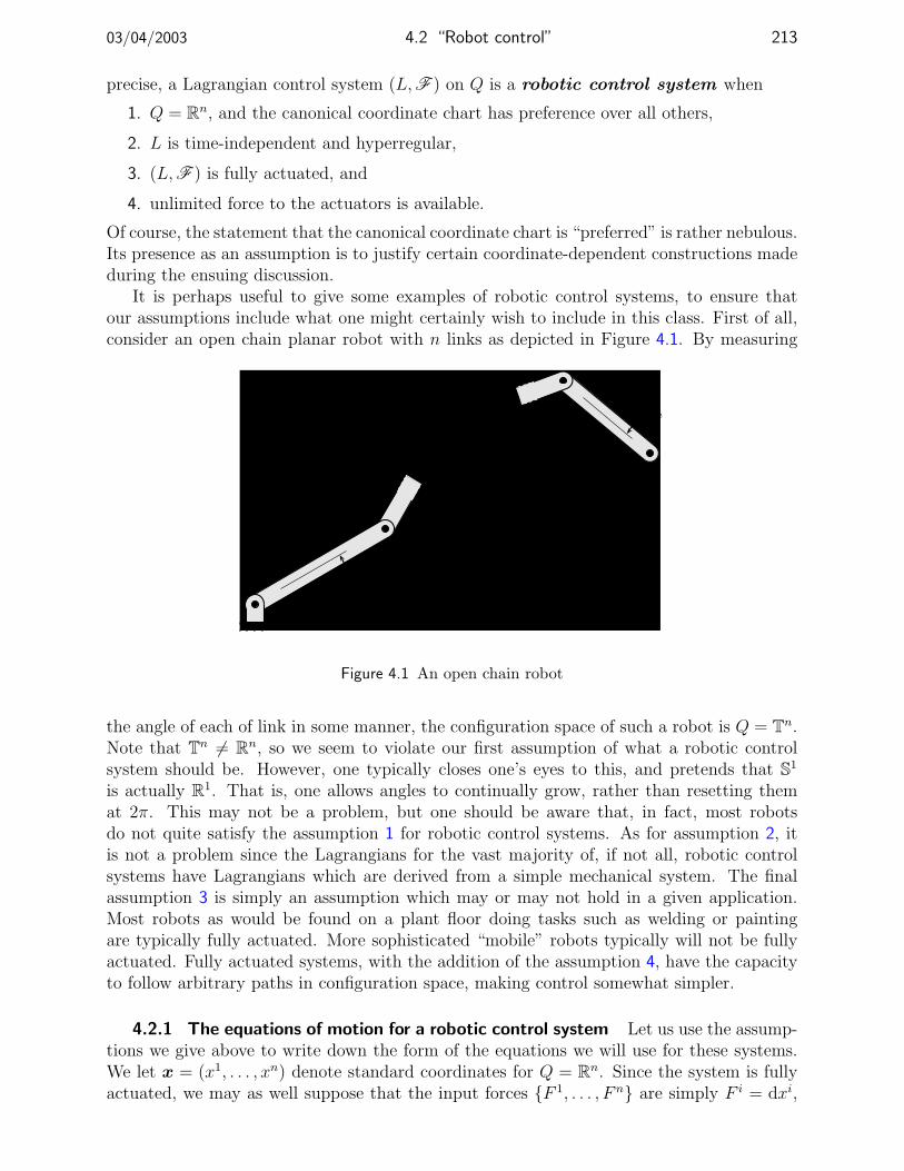
03/04/2003 4.2 “Robot control” 213
precise, a Lagrangian control system (L,F ) on Q is a robotic control system when
1. Q = Rn, and the canonical coordinate chart has preference over all others,
2. L is time-independent and hyperregular,
3. (L,F ) is fully actuated, and
4. unlimited force to the actuators is available.
Of course, the statement that the canonical coordinate chart is “preferred” is rather nebulous.Its presence as an assumption is to justify certain coordinate-dependent constructions madeduring the ensuing discussion.
It is perhaps useful to give some examples of robotic control systems, to ensure thatour assumptions include what one might certainly wish to include in this class. First of all,consider an open chain planar robot with n links as depicted in Figure 4.1. By measuring
θ1
θn
Figure 4.1 An open chain robot
the angle of each of link in some manner, the configuration space of such a robot is Q = Tn.Note that Tn 6= Rn, so we seem to violate our first assumption of what a robotic controlsystem should be. However, one typically closes one’s eyes to this, and pretends that S1
is actually R1. That is, one allows angles to continually grow, rather than resetting themat 2π. This may not be a problem, but one should be aware that, in fact, most robotsdo not quite satisfy the assumption 1 for robotic control systems. As for assumption 2, itis not a problem since the Lagrangians for the vast majority of, if not all, robotic controlsystems have Lagrangians which are derived from a simple mechanical system. The finalassumption 3 is simply an assumption which may or may not hold in a given application.Most robots as would be found on a plant floor doing tasks such as welding or paintingare typically fully actuated. More sophisticated “mobile” robots typically will not be fullyactuated. Fully actuated systems, with the addition of the assumption 4, have the capacityto follow arbitrary paths in configuration space, making control somewhat simpler.
4.2.1 The equations of motion for a robotic control system Let us use the assump-tions we give above to write down the form of the equations we will use for these systems.We let x = (x1, . . . , xn) denote standard coordinates for Q = Rn. Since the system is fullyactuated, we may as well suppose that the input forces F 1, . . . , F n are simply F i = dxi,

214 4 An introduction to control theory for Lagrangian systems 03/04/2003
i = 1, . . . , n. Let us denote this set of forces by Fcan. The Euler-Lagrange equations arethen
∂2L
∂vi∂vjxj +
∂2L
∂vi∂xjxj − ∂L
∂xi= ui, i = 1, . . . , n.
If we define a symmetric invertible matrix function M : Rn×Rn → Rn×n to have components∂2L
∂vi∂vj , i, j = 1, . . . , n, and if we define a map N : Rn × Rn → Rn by
N (x,v)i =∂2L
∂vi∂xjxj − ∂L
∂xi, i = 1, . . . , n,
then the equations of motion can be written
M(x, x)x + N (x, x) = u. (4.2)
Let us specialise the notation further to the situation when the Lagrangian L is derivedfrom a simple mechanical system (Q, g, V ), which will most often be the case. In this caseone readily sees, first of all, that M is independent of v, and indeed is simply the matrix ofcomponents for the Riemannian metric g in the standard coordinates for Rn. The term Ncan also be effectively broken down. We define a map C : Rn → L(Rn × Rn; Rn) by
C(x)(v1,v2)i =1
2
(∂M ij
∂xk+∂M ik
∂xj− ∂M jk
∂xi
)vj
1vk2 .
Thus C is related in a simple way to the Christoffel symbols for the Riemannian metric g inthe standard coordinates. If dV is the vector of partial derivatives of the potential functionV , then the equations (4.2) specialise to the equations
M(x)x + C(x)(x, x) + dV = u. (4.3)
The term C(x)(x, x) is often given the name “Coriolis forces.” Note that we violate our codeof coordinate invariance in writing these equations. Indeed, in Remark 2.4.12 we explicitlyadvised against writing equations in the form (4.3)! However, we justify what we havedone by saying that we have used our assumption 1 for a robotic control system where thestandard coordinates for Q are preferred. Also, since we are supposed to be talking aboutrobot control, we may as well do as most robot control folks do, and write the equationsas (4.2) or (4.3).
Before we move on, let us give a useful property of the notation used in (4.3).
4.2.1 Lemma With M and C as used in (4.3) we have xtMx− 2xt(C(x)(x, x)
)= 0.
Proof We compute
M ij =∂M ij
∂xkxk.
It is then a straightforward computation using the definition of C to verify that
xtMx− 2xt(C(x)(x, x)
)=(∂M jk
∂xixk − ∂M ik
∂xjxk)xixj.
Since the expression in the brackets is skew-symmetric with respect to the indices i and j,the result follows.
Lewis [1997] gives an interpretation of this result in terms of conservation of energy.

03/04/2003 4.2 “Robot control” 215
4.2.2 Feedback linearisation for robotic systems The title of this section is a bitpretentious. What we talk about in this section is sometimes referred to as the “computedtorque” control law. It is, however, an example of a more general technique known asfeedback linearisation, and this is why the title is as it is.
The setup for the computed torque control law, like that for the PD control law in thenext section, is that one has a robotic control system (L,Fcan) on Q, and a desired trajectoryt 7→ xdes(t) for the configuration of the system. If the actual robot is evolving according toa curve t 7→ x(t) in configuration space, the error , t 7→ e(t), is then the difference betweenwhere one is and where one wants to be:
e(t) = x(t)− xdes(t).
The idea is that one wishes to design a control law u for (4.2) so that the error goes to zeroas t→∞. The computed torque control law is defined by
uCT = M(x, x)xdes + N (x, x)−M(x, x)(Kve + Kpe
),
where Kv,Kp ∈ Rn×n are matrices, designed so as to accomplish a stated objective. Let usfirst get the form of the error dynamics using the computed torque control law.
4.2.2 Proposition Let t 7→ xdes(t) be a curve in Rn. With u(t) = uCT(t) in (4.2), the errore(t) = x(t)− xdes(t) satisfies the differential equation
e(t) + Kve(t) + Kpe(t) = 0.
Proof Substituting uCT into (4.2), some straightforward manipulation yields
M(x, x)(e(t) + Kve(t) + Kpe(t)
)= 0.
The result follows since M(x,v) is invertible for all v and v.
Now it is a simple matter to give a general form for Kv and Kp so that the error dynamicsgo to zero at t→∞.
4.2.3 Proposition If Kv and Kp are symmetric and positive-definite, then the error dynamicsin Proposition 4.2.2 satisfy limt→∞ e(t) = 0.
Proof Writing the differential equation for the error in first-order form gives(e
f
)=
[0 In
−Kp Kv
](ef
),
where f = e. The result will follow if we can show that all eigenvalues of the matrix
A =
[0 In
−Kp Kv
]have negative real part. Let λ ∈ C be an eigenvalue with eigenvector (v1,v2) ∈ Cn × Cn.We must then have (
v2
−Kpv1 −Kvv2
)=
(λv1
λv2
).

216 4 An introduction to control theory for Lagrangian systems 03/04/2003
Let 〈·, ·〉 be the standard inner product on Cn: 〈z1, z2〉 = zt1z2, where · means complex
conjugation. We then have⟨λz1, λv1
⟩=⟨λz1,v2
⟩= 〈v1, λv2〉= 〈v1,−Kpv1 −Kvv2〉= − 〈v1,Kpv1〉 − λ 〈v1,Kvv1〉 .
We also have⟨λz1, λv1
⟩= λ2 〈v1,v1〉, thus giving us
〈v1,v1〉λ2 + 〈v1,Kvv1〉λ+ 〈v1,Kpv1〉 = 0.
Now note that if v1 = 0 then we also have v2 = 0. Since eigenvectors are necessarilynonzero, this implies that v1 6= 0. Thus λ satisfies the equation
aλ2 + bλ+ c = 0,
where a > 0 since v1 6= 0, and where b, c > 0 since Kp and Kv are symmetric and positive-definite. We therefore conclude that λ has strictly negative real part, as desired.
The computed torque control law has the advantage, therefore, of being able to trackaccurately any desired reference trajectory. To do so, however, may require significantactuator forces. Nevertheless, it is an effective control strategy.
4.2.3 PD control It is possible to use some simple ideas from classical control forrobotic systems, and perhaps the simplest controller which might be effective is PD control,or Proportional-Derivative control. Here one simply defines the control to be the sum oftwo terms, one proportional to the error, and one proportional to the derivative of the error.That is, for a given desired trajectory t 7→ xdes(t) in Q, we define
uPD(t) = −Kpe(t)−Kve(t),
for symmetric positive-definite matrices Kp,Kv ∈ Rn×n, and where e(t) = x(t) − xdes(t),as before. The PD control law is not as effective as the computed torque controller forfollowing arbitrary reference trajectories. This is a general failing of PD controllers, oftenalleviated by implementing integral control. However, the following result indicates thata PD controller will stabilise a robotic control system to a desired configuration when theLagrangian is derived from a simple mechanical system. Since almost all robotic systemsare in practice of this form, this is not at all a significant restriction.
4.2.4 Proposition Let (L,Fcan) be a robotic control system with L the Lagrangian for thesimple mechanical system (Q, g, 0) with zero potential energy. If t 7→ xdes(t) = x0 is aconstant desired trajectory, then taking u(t) = uPD(t) in (4.3) gives limt→∞ e(t) = 0.
Proof We will use the LaSalle Invariance Principle to show that x0 is an asymptoticallystable equilibrium point for (4.3) if we take u = uPD. First note that the equations (4.3)with u = uPD are
M(x)x + C(x)(x, x) + Kvx + Kp(x− x0) = 0. (4.4)

03/04/2003 4.3 Passivity methods 217
Now define a Liapunov function on Q by
G(x,v) =1
2vtM(x)v +
1
2(xt − xt
0)Kp(x− x0).
We compute
G(x, x) = xM (x)x +1
2xM(x)x + xKp(x− x0)
= − x(C(x)(x, x)
)+
1
2xM(x)x− xtKvx
= − xtKvx.
Here we have used Lemma 4.2.1. Note that the closed-loop equations (4.4) are forced Euler-Lagrange equations with Lagrangian
L(x,v) = L(x,v)− 1
2(xt − xt
0)Kp(x− x0).
and with external force F (x,v) = Kvv. This force is strictly dissipative so we apply theLaSalle Invariance Principle. The LaSalle Invariance Principle states that the system willtend towards the set where F (x,v) · v = 0. However, this set is comprised of those pointsin TQ where v = 0. Now we note, again with the LaSalle Invariance Principle in mind, thatthe largest invariant set for L for which v = 0 is the set of critical points for L of the form(x,0). However, for such critical points x must be a critical point for the potential function
V (x) =1
2(xt − xt
0)Kp(x− x0).
Since x0 is the only critical point for V , the result follows from Corollary 3.5.7.
Murray, Li and Sastry [1994] provide an extension of the PD control we have definedhere which allows one to asymptotically track general reference trajectories. Also, the ideasbehind what we suggest here can be extended in a geometric framework which alleviatessome of the inherent restrictions of the PD control we suggest in this section. We refer thereader to [Koditschek 1989, Bullo and Murray 1999] for ideas along these lines.
4.3 Passivity methods
Sorry, not this year. See [Ortega, Loria, Nicklasson and Sira-Ramirez 1998].
4.4 Linearisation of Lagrangian control systems
The material in the previous section was geared towards fully actuated systems, anda special class of these, even. When confronted with a system with fewer controls thandegrees of freedom, things become more difficult. For certain control problems, notably thepoint stabilisation problem, a good thing to try first is linearisation, just as when studyingdynamics.
4.4.1 The linearised system When linearising (4.1), one wishes to linearise both withrespect to control and state. In Section 3.2 we already linearised the left hand side of (4.1),

218 4 An introduction to control theory for Lagrangian systems 03/04/2003
so it only remains to linearise the terms with the control. This, however, is trivial since thisterm is already linear in the control. Therefore, when linearising, one need only substitutethe value of the equilibrium point into the forces. With this as motivation, we make thefollowing definition.
4.4.1 Definition Let (L,F ) be a Lagrangian control system on Q and let q0 be an equilibriumpoint for L. The linearisation of (L,F ) is the quadruple (ML(q0), CL(q0), KL(q0),F (q0))where ML(q0), CL(q0), and KL(q0) are as defined in Proposition 3.2.10, and where F (q0) =F 1(0q0), . . . , F
m(0q0) ⊂ T ∗q0Q.
Corresponding to the linearisation is the following linear control system on Tq0Q:
ML(q0)q(t) + CL(q0)q(t) +KL(q0)q(t) = uaFa(0q0),
where t 7→ q(t) is a curve on Tq0Q. (We make a nasty abuse of notation here, so beware:we let q denote both points in Q and points in Tq0Q.) In the same way as we did whenlinearising near equilibria in studying dynamics, let us suppose that L is hyperregular sothat M ]
L(q0) is invertible. In this case, let us define a linear map BL(q0) : Rm → Tq0Q by
BL(q0)(u1, . . . , um) = u1M]L(q0)
(F 1(0q0)
)+ · · ·+ umM
]L(q0)
(Fm(0q0)
).
We then arrive at the linear control system on Tq0Q⊕ Tq0Q given by(qv
)=
[0 idV
−M ]L(q0) K
[L(q0) −M ]
L(q0) C[L(q0)
](qv
)+
(0
BL(q0)
)u.
This is a linear control system in the best tradition. That is to say, it is a time-invariantsystem of the form
x = Ax+Bu
where
x =
(qv
)A = AL(q0) =
[0 idV
−M ]L(q0) K
[L(q0) −M ]
L(q0) C[L(q0)
]B = BF (q0) ,
(0
BL(q0)
).
There is an exorbitant amount of literature on such systems [e.g., Brockett 1970], and weonly address a few of the more basic notions for such systems. Our emphasis, like it waswhen we were dealing with dynamics, is on deciding the relationship between the linearisedsystem and the actual system near the equilibrium point in question.
4.4.2 Controllability of the linearised system A first basic question deals with con-trollability. The reader will recall that a linear control system
x = Ax+Bu,
where t 7→ x(t) is a curve in a vector space V , is controllable if for any x1, x2 ∈ V thereexists a control u : [0, T ] → Rm so that if the initial condition is x(0) = x1, then x(T ) = x1.

03/04/2003 4.4 Linearisation of Lagrangian control systems 219
In brief, the system is controllable if it can be steered from any state to any other state. TheKalman rank condition says that the system is controllable if and only if the matrix[
B AB · · · AN−1B]
has rank equal to N = dim(V ), where A ∈ RN×N and B ∈ RN×m are the matrix represen-tations of A and B in some basis for V .
Let us see how this transfers to our Lagrangian setting. The first result we state is themost general, and to state it requires some notation. Let I be the collection of multi-indices in 1, 2. Thus an element I ∈ I has the form I = (i1, . . . , ik) where ia ∈ 1, 2 fora = 1, . . . , k. For a multi-index I, we write |I| for its length. Thus |(i1, . . . , ik)| = k. For amulti-index I ∈ I we denote by |I|1 the number of 1’s in I, and by |I|2 the number of 2’sin I. Note that |I|1 + |I|2 = |I|. Now suppose that we choose a basis for Tq0Q and denote
by A1(q0),A2(q0) ∈ Rn×n the matrices of M ]L(q0) K
[L(q0) and M ](q0) C
[L(q0), respectively,
with respect to this basis. Now for k ∈ Z+ define
Rn×n 3 M (k)(q0) =
k∑j=k/2
∑|I|=j
|I|1=k−j
Ai1(q0) · · ·Aij(q0), k even
k∑j=(k+1)/2
∑|I|=j
|I|1=k−j
Ai1(q0) · · ·Aij(q0), k odd.
Let us give the first few of the matrices M (k)(q0) so that the reader might begin to understandthe cumbersome notation. We determine that
M (1)(q0) = A2(q0)
M (2)(q0) = A1(q0) + A2(q0)2
M (3)(q0) = A1(q0)A2(q0) + A2(q0)A1(q0) + A2(q0)3
M (4)(q0) = A1(q0)2 + A1(q0)A2(q0)
2 + A2(q0)A1(q0)A2(q0) + A2(q0)2A1 + A2(q0)
4.
Hopefully this is enough to enable the reader to see how one proceeds, using the definitionsfor M (k)(q0). k > 0.
With this notation in hand, we may state our main result concerning controllability oflinearisations.
4.4.2 Theorem Let (L,F ) be a Lagrangian control system on Q with L a hyperregular La-grangian. Let q0 be an equilibrium point for L and let (ML(q0),CL(q0),KL(q0),F (q0)) bethe linearisation of (L,F ) at q0. The linearised system
x = AL(q0)x + BF (q0)u
is controllable if and only if the matrix[B(q0) M(1)(q0)B(q0) · · · M(2n−2)(q0)B(q0)
]has rank 2n, where M(k)(q0), k = 1, . . . , 2n − 2 are as defined above with respect to somebasis for Tq0Q, and where B(q0) is the matrix of BL(q0) with respect to the same basis.

220 4 An introduction to control theory for Lagrangian systems 03/04/2003
Proof The following lemma contains the bulk of the idea of the tedious proof.
1 Lemma Let A ∈ R2n×2n and B ∈ R2n×m be given by
A =
[0 In
A1 A2
], B =
[0B2
],
for A1,A2 ∈ Rn×n and B2 ∈ Rn×m. Let M(0) = In and for k ∈ Z+ define
M(k) =
k∑j=k/2
∑|I|=j
|I|1=k−j
Ai1 · · ·Aij , k even
k∑j=(k+1)/2
∑|I|=j
|I|1=k−j
Ai1 · · ·Aij , k odd.
Then, for k ∈ Z+ we have
AkB =
[M(k−1)B2
M(k)B2
].
Proof For k = 1 we have M (1) = A2 so that(M (0)B2
M (1)B2
)=
(B2
A2B2
).
One readily verifies now that the lemma holds for k = 1. Suppose it true for k > 1. Wethen have
Ak+1B =
(M (k)B2
A1M(k−1)B2 + A2M
(k)B2
).
First let us suppose that k is even. In this case we have
A1M(k−1) + A2M
(k) =k−1∑
j=k/2
∑|I|=j
|I|1=k−j−1
A1Ai1 · · ·Aij +k∑
j=k/2
∑|I|=j
|I|1=k−j
A2Ai1 · · ·Aij
=k−1∑
j=k/2
∑|I|=j
|I|1=k−j−1
A1Ai1 · · ·Aij +k−1∑
j=k/2
∑|I|=j
|I|1=k−j
A2Ai1 · · ·Aij + Ak+12
=k∑
j=(k+2)/2
∑|I|=j
|I|1=k−j+1
Ai1 · · ·Aij + Ak+12
=k∑
j=(k+2)/2
∑|I|=j
|I|1=k−j+1
Ai1 · · ·Aij
= M (k+1).
A similarly styled computation also shows that A1M(k−1) + A2M
(k) = M (k+1) when k isodd. This now gives the result. H

03/04/2003 4.4 Linearisation of Lagrangian control systems 221
To proceed with the proof of the theorem, note that the situation dealt with in thetheorem is just as in the lemma with A1 = −A1(q0), A2 = −A2(q0), and B2 = B(q0).Furthermore, by the lemma we have
[B AB A2B · · · A2n−1B
]=
[0 B2 M (1)B2 · · · M (2n−2)B2
B2 M (1)B2 M (2)B2 · · · M (2n−1)B2
].
Let us define M 1,M 2 ∈ R2n×2nm by
M 1 =[
0 B2 M (1)B2 · · · M (2n−2)B2
]M 2 =
[B2 M (1)B2 M (2)B2 · · · M (2n−1)B2
].
Note image(M 1) ⊂ image(M 2). Therefore the rank of[M 1
M 2
]will equal 2n if and only if rank(M 1) = n, as stated.
Let us now specialise the above theorem to the important case when CL(q0) = 0. In thiscase, with our above notation with respect to a basis for Tq0Q, we have A2(q0) = 0. We nowshow, using Theorem 4.4.2, that the following condition for controllability of the linearisedsystem holds.
4.4.3 Corollary Let (L,F ) be a Lagrangian control system on Q with L a hyperregular La-grangian. Let q0 be an equilibrium point for L and let (ML(q0),CL(q0),KL(q0),F (q0)) bethe linearisation of (L,F ) at q0, supposing that CL(q0) = 0. The linearised system
x = AL(q0)x + BF (q0)u
is controllable if and only if the matrix[B(q0) A1(q0)B(q0) · · · An−1
1 (q0)B(q0)]
has rank n, where A2(q0) is the matrix of M]L(q0) K
[L(q0) with respect to some basis for
Tq0Q, and where B(q0) is the matrix of BL(q0) with respect to the same basis.
Proof One verifies using the definition of M (k)(q0) above, with A2(q0) = 0, that
M (k)(q0) =
0, k odd
A1(q0)k/2, k even.
The result now follows directly from Theorem 4.4.2.
4.4.4 Remark Corollary 4.4.3 holds in the important case where q0 is an equilibrium point fora simple mechanical system since, by Proposition 3.3.7, CL(q0) = 0 at equilibrium points forsimple mechanical systems. Also note that the condition for controllability of the linearisedsystem simplifies significantly in this case since the matrix whose rank needs to be checkedis essentially half the size.
Let us look at a simple example on the basis of the previous remark.
222 4 An introduction to control theory for Lagrangian systems 03/04/2003
4.4.5 Example (Example 2.6.3 cont’d) We consider the pendulum of Example 2.6.3, and nowapply a torque at the base of the pendulum. One might intuitively expect the system to becontrollable, but let us perform the linearisation analysis, just so we know how it goes.
The Lagrangian for the system we take to be L(q, v) = m`2 12v2 +m`ag cos q. Note that
we reinsert units into the problem to make it a little more interesting. The Euler-Lagrangeequations, with the torque at the base of the pendulum denoted by u, read
m`2q +m`ag sin θ = u.
There are two equilibrium points, q1 = 0 and q2 = π. We compute the linearisations of L atthese points to be
ML(q1) = m`2, KL(q1) = m`ag
ML(q2) = m`2, KL(q2) = −m`ag,
with CL(q1) = CL(q2) = 0 by virtue of the system being a simple mechanical system. Wethen determine that
M ]L(q1) K
[L(q1) =
ag
`, M ]
L(q2) K[L(q2) = −ag
`.
We also have BL(q1) = BL(q2) = 1m`2
. Now, adopting the notation of Corollary 4.4.3, wefind that [
B(q1) A1(q1)B(q1)]
=[
1m`2
ag
m`
][B(q2) A1(q2)B(q2)
]=[
1m`2
− ag
m`
].
In each case, of course the rank of the matrix has maximal rank 1. This example is perhapstoo trivial to illustrate much, and the reader is encourage to try out the results on the moreinteresting examples in the exercises.
An important corollary is the following which deals with simple mechanical systems withno potential. Recall that for such systems, every point q0 ∈ Q is an equilibrium point.
4.4.6 Corollary Let (L,F ) be a Lagrangian control system with L the Lagrangian for a sim-ple mechanical system (Q, g, 0) with zero potential. For any q0 ∈ Q, the linearisation(ML(q0),CL(q0),KL(q0),F (q0)) is controllable if and only if (L,F ) is fully actuated.
Proof In the notation of Theorem 4.4.2, A1(q0) = A2(q0) = 0. Therefore, using Corol-lary 4.4.3 the system is controllable if and only if the matrix B(q0) has rank n. But this willhappen if and only if
spanRF 1(0q0), . . . , F
m(0q0)
= Tq0Q.
By our assumption of the independence of the dimension of the span of the forcesF 1(vq), . . . , F
m(vq) on vq ∈ TQ, the result follows.
This result has important implications. It says that one cannot expect anything helpfulto occur when linearising a simple mechanical system with a kinetic energy Lagrangian,except in the trivial case when we have full authority available to us with the controls. Inthese cases, we may resort to the methods of Section 4.2. In other cases, when the systemis underactuated, things become rather complicated, and we mention a few “simple” ideasin Section 4.5.

03/04/2003 4.4 Linearisation of Lagrangian control systems 223
Let us give another important application of Theorem 4.4.2. Let us suppose that wehave a system which is subjected to a dissipative force which is linear in velocity, as is thecase with viscous friction. The force we consider is thus of the form
F (vq) = −R[q(vq)
where Rq is a positive semi-definite quadratic form on TqQ. Note that this is simply ageneralisation of the viscous force given in a simple example in Example 2.5.9–1. With adissipative force of this type, an equilibrium point for L will still be an equilibrium point withthe addition of the dissipative force since this force vanishes when velocity is zero. Therefore,we may still linearise about equilibria for L, even in the presence of this dissipative force. Todetermine the controllability of the linearisation, we need a comparatively straightforwardmodification of the notation used in Theorem 4.4.2. Let A1(q0) = A1(q0) be as used inthat theorem, and let A2(q0) be the matrix for the linear map M ]
L(q0) (C[L(q0) +R[
q0). Now
define
Rn×n 3 M (k)(q0) =
k∑j=k/2
∑|I|=j
|I|1=k−j
Ai1(q0) · · · Aij(q0), k even
k∑j=(k+1)/2
∑|I|=j
|I|1=k−j
Ai1(q0) · · · Aij(q0), k odd.
The following result tells us when the resulting linearisation of a system with viscousdissipation is controllable.
4.4.7 Proposition Let (L,F ) be a Lagrangian control system on Q with L a hyperreg-ular Lagrangian, and let F be a dissipative force on Q of the form F(vq) = R[
q(vq),with Rq positive semi-definite, as above. If q0 is an equilibrium point for L, let(ML(q0),CL(q0),KL(q0),F (q0)) be the linearisation of (L,F ). The linearisation of thesystem with the addition of the dissipative force F is controllable if and only if the matrix[
B(q0) M(1)(q0)B(q0) · · · M(2n−2)(q0)B(q0)]
has rank 2n, where M(k)(q0), k = 1, . . . , 2n − 2 are as defined above with respect to somebasis for Tq0Q, and where B(q0) is the matrix of BL(q0) with respect to the same basis.
Proof We shall compute the linearisation of the system at the equilibrium point q0. We dothis by working in coordinates (q1, . . . , qn). Following the computations preceding Proposi-tion 3.2.10, we Taylor expand about (q0,0). The resulting expression is
∂2L
∂vj∂viξj(t) +
( ∂2L
∂qj∂vi− ∂2L
∂vj∂qi
)ξj(t)− ∂2L
∂qj∂qiξj(t) + · · · =
−Rij(q0)ξj(t) + uaF
ai (q0,0), i = 1, . . . , n,
where ξi(t) = qi(t)− qi0, i = 1, . . . , n. Thus the linearised equations look like
ML(q0)q + CL(q0)q +KL(q0)q = −R[q0
(q) + uaFa(0q0).
Here again we make the horrific abuse of notation of writing points in the tangent spaceTq0Q as q. Using the fact that L is hyperregular, we write these as first-order equations:(
qv
)=
[0 idV
−M ]L(q0) K
[L(q0) −M ]
L(q0) (C[L(q0) +R[
q0)
](qv
)+
(0
BL(q0)
)u.
The result now follows directly from Lemma 1 of the proof of Theorem 4.4.2.

224 4 An introduction to control theory for Lagrangian systems 03/04/2003
4.4.3 On the validity of the linearised system The previous section dealt with thelinearisation of a Lagrangian system. However, given our discussion of Section 3.2 on lineari-sation as it relates to dynamics near equilibrium points, one would be well-justified in beingsuspicious about cavalierly making conclusions about Lagrangian control systems based uponproperties of their linearised systems.
Things, however, are not as grim as they might be. The following result is Proposition 3.3of [Nijmeijer and van der Schaft 1990], but translated into our context.
4.4.8 Theorem Let (L,F ) be a Lagrangian control system with hyperregular Lagrangian L, letq0 be an equilibrium point for L, and let (ML(q0),CL(q0),KL(q0),F (q0)) be the linearisationof (L,F ) at q0. If the linearised system is controllable, then for every T, ε > 0 the set ofpoints in TQ reachable from 0q0 in time T using controls satisfying ‖u(t)‖ < ε, t ∈ [0,T],contains a neighbourhood of 0q0.
In other words, if the linearisation at q0 is controllable, then the system is controllable forsmall times, and for small controls, near q0. This result is important, because it suggests thatit may be valid to use the linear approximation, as long as we remain near the equilibriumpoint. Indeed, this is a very common technique for controlling systems near equilibriumpoints.
The converse of the question dealt with by Theorem 4.4.8, however, is not so straight-forward. That is, it is certainly not true that if a system is controllable near q0 then itslinearisation is also controllable. To determine the controllability properties of such systems,one must resort to nonlinear methods. It is towards this that we now turn our attention.
4.5 Control when linearisation does not work
In this section we give a crude flavour to the problem of how to attack the control problemfor a mechanical system when one has found that the linearisation is not controllable. It isbeyond the scope of what we are doing to deal in any depth with the problems here, andtherefore we give only a brief sketch of some of the existing technology, and point the readerto the appropriate literature.
4.5.1 Driftless nonlinear control systems As a preparation to the techniques wewill use to control mechanical systems, we look at a class of nonlinear system which is notmechanical. A driftless control system is a pair Σ = (Q,X ) where X = X1, . . . , Xsis a collection of vector fields on Q. The control system we consider is given by
c′(t) = uα(t)Xα(c(t)). (4.5)
The controls we consider are, say, piecewise differentiable, although we may use more generalcontrols. A controlled trajectory for a driftless system Σ = (Q,X ) is a pair (c, u) whereu : [0, T ] → Rs is piecewise differentiable, and where c : [0, T ] → Q is such that the differentialequation (4.5) is satisfied. We shall make the assumption that the dimension of the subspaceXq defined by
Xq = spanR X1(q), . . . , Xs(q)
is independent of q.It is possible to give a complete description of controllability for such systems. First
let us describe the type of controllability we consider. The driftless system X1, . . . , Xs is

03/04/2003 4.5 Control when linearisation does not work 225
controllable if for q1, q2 ∈ Q there exists a controlled trajectory (c, u) defined on the interval[0, T ] with the property that c(0) = q1 and c(T ) = q2. To determine the controllabilityconditions we let L(X ) be the smallest subset of vector fields on Q with the property thatX ⊂ L(X ) and with the property that [X, Y ] ∈ L(X ) for all vector fields X, Y ∈ L(X ).Now, for each q ∈ Q, define a subspace Lie(X )q by
Lie(X )q = X(q) | X ∈ L(X ) .
To compute L(X ) in practice, it often suffices to iterative take Lie brackets of the vectorfields X1, . . . , Xs until one stops generating new directions. Thus one computes the vectorfields [Xa, Xb], a, b = 1, . . . , s, [Xa, [Xb, Xc]], a, b, c = 1, . . . , s, and so on. Typically thisprocess will “terminate” in the sense that Lie(X )q will stop growing.
The following important result gives conditions on when a driftless system is controllable.
4.5.1 Theorem (Chow [1939]) A driftless control system Σ = (Q,X ) is controllable ifLie(X )q = TqQ for each q ∈ Q. If the vector fields X are real analytic, then this conditionis also necessary.
Let us make some general comments concerning driftless systems.
4.5.2 Remarks 1. We name driftless systems as we do because they are a specific case ofcontrol systems of the type
c′(t) = X0(c(t)) + uα(t)Xα(c(t)),
where we now have no control over the vector field X0, which is called the drift vectorfield . For driftless systems, of course, the drift vector field is zero. Systems with nonzerodrift vector fields are significantly harder to deal with. In particular, there are no knownnecessary and sufficient conditions for controllability of the type given in Theorem 4.5.1for systems with drift.
2. Note that equation (4.5) essentially describes the set of curves t 7→ c(t) whose tangentvectors lie in c′(t) lie in the subspace spanR X1(c(t)), . . . , Xs(c(t)) for each t. In thisway, one can think of (4.5) as describing a linear constraint on Q, exactly as we didin Section 2.6. With this interpretation, Theorem 4.5.1 gives conditions on when it ispossible to connect any two points in Q with a curve satisfying the constraint.
3. If one linearises (4.5) about a point q0, the resulting linear control system on Tq0Q issimply
q(t) = B(q0)u,
where B(q0) : Rs → Tq0Q is defined by B(q0)u = uαXα(q0). The Kalman rank condition(the “A” matrix is zero) tells us that this linearisation is stable if and only if B(q0) issurjective, i.e., if the tangent vectors X1(q0), . . . , Xs(q0) generate Tq0Q. Thus the systemis controllable only in the trivial case where the inputs allow us to access all directionsin Q.
Now that we have dealt with the controllability question for driftless systems, let uslook at how to handle some common control problems. First let us look at the problem ofdesigning a control law which will stabilise the system to a desired point q0. The followingresult states that the upshot of the observation Remark 4.5.2–3 is fatal as far as usingfeedback to stabilise a driftless system.

226 4 An introduction to control theory for Lagrangian systems 03/04/2003
4.5.3 Theorem (Brockett [1983]) Let q0 ∈ Q. It is not possible to define a continuous func-tion u: Q → Rs with the property that the closed-loop system for (4.5),
c′(t) = uα(c(t))Xα(c(t)),
has q0 as an asymptotically stable fixed point.
The theorem states that if we wish to use a closed-loop controller to stabilise the sys-tem (4.5), then the feedback must either be discontinuous, or time-dependent. Both ap-proaches have been tried in the literature with some success. The papers [Sontag 1999, Bac-ciotti and Ceragioli 1999] provide a review of the use of discontinuous feedback to stabilisean equilibrium point. One of the problems surrounding the use of discontinuous feedbackis that it becomes an issue to decide in what sense solutions are to be defined. The mostcommon notion is “the sense of Fillipov” [Filippov 1984], but ideas of Clarke, [Clarke 1983]and [Clarke, Ledyaev, Stern and Wolenski 1998], are also important.
When talking about stabilisation of driftless systems, the notion of “homogeneity” is im-portant. A recent paper with an excellent survey of such issues in the introduction is [Morin,Pomet and Samson 1999]. In that paper will also be found an algorithm for providing a sta-bilising control law based on the method of homogeneous approximation. Coron and Rosier[1994] show, roughly, that if a system can be stabilised by discontinuous feedback, then itcan be stabilised by time-varying feedback.
Now let us turn to reviewing the literature concerning the question of constructing acontrol law which steers the system from one point to another. Of course, before attemptingsuch a thing, one must ensure that the system is controllable. The state of knowledgehere is not as advanced as it is for the stabilisation problem, and a review of what isknown is presented in Chapter 8 of [Murray, Li and Sastry 1994]. The paper [Murray andSastry 1993] gives a methodology of using sinusoids to steer a class of systems. The classof systems are somewhat restricted, but it is sometimes possible to put a given system intothe required form. Lafferriere and Sussmann [1991] provide another methodology based on“nilpotent approximations.” The methods here may be useful in the context of kinematicallycontrollable systems which we discuss in Section 4.5.4.
4.5.2 Affine connection control systems The mechanical systems we consider are animportant subclass of Lagrangian control systems whose Lagrangians are those for a simplemechanical system (Q, g, 0) with zero potential. We also make the assumption that the inputforces are independent of time and velocity. Thus the input forces F = F 1, . . . , Fm aresimply one-forms on Q. As we saw in Proposition 2.5.10, the equations which govern themotion of this control system are then
g
∇c′(t)c′(t) = ua(t)g
](F a(c(t))),
whereg
∇ is the Levi-Civita connection associated with g. It turns out that we loose nothingby generalising to the situation where the connection is arbitrary, and the inputs are arbitraryvector fields. To this end, we say that an affine connection control system is a tripleΣaff = (Q,∇,Y ) where ∇ is an affine connection on Q, and Y = Y1, . . . , Ym are vectorfields on Q. The control equations are then, of course,
∇c′(t)c′(t) = ua(t)Ya(c(t)). (4.6)
03/04/2003 4.5 Control when linearisation does not work 227
A controlled trajectory for an affine connection control system is a pair (c, u) whereu : [0, T ] → Rm is piecewise differentiable, and where c : [0, T ] → Q has the property thatthe differential equation (4.6) is satisfied. The act of even defining appropriate notions ofcontrollability for (4.6) requires some ideas we do not wish to deal with in full generality [seeLewis and Murray 1997]. Let us agree to deal only with the simplified notion of controllabilitycalled equilibrium controllability where the system possesses this property if for eachq1, q2 ∈ Q, there exists a controlled trajectory (c, u) defined on the interval [0, T ] with theproperty that c′(0) = 0q1 and c′(T ) = 0q2 . Roughly, the system is equilibrium controllablewhen it can be steered from any point at rest to any other point at rest. As we have beendoing all along, we shall assume that the dimension of the subspace
Yq = spanR Y1(q), . . . , Ym(q)
is independent of q.Note that (4.6) has a form somewhat similar to the equation (4.5) for driftless systems.
However, the two types of systems are in no way the same! For example, the equations (4.6)are second-order, whereas the equations (4.5) are first-order. Despite the fact that the twotypes of equations are not equivalent, in some examples they are related in some way, andit is this fact which we will exploit in the remainder of the section.
4.5.3 Mechanical systems which are “reducible” to driftless systems It turns outthat some, but certainly not all (in some sense very few indeed), mechanical systems can, ina limited sense, be thought of as driftless systems. Fortunately, these systems are ones forwhich linearisation is ineffective, so the connection with driftless systems provides an “in”to being able to do some control tasks for these systems.
The following definition establishes the type of correspondence we are after in this sec-tion.
4.5.4 Definition Let Σaff = (Q,∇,Y ) be an affine connection control system and let Σ =(Q,X ) be a driftless system. Σaff is reducible to Σ if the following two conditions hold:
(i) for each controlled trajectory (c, u) for Σ defined on [0, T ] with u differentiable andpiecewise C2, there exists a piecewise differentiable map u : [0, T ] → Rm so that (c, u)is a controlled trajectory for Σaff;
(ii) for each controlled trajectory (c, u) for Σaff defined on [0, T ] and with c′(0) ∈ Xq, thereexists a differentiable and piecewise C2 map u : [0, T ] → Rs so that (c, u) is a controlledtrajectory for Σ.
The idea of the definition is quite simple. It establishes that there is a correspondencebetween controlled trajectories for the driftless system and the affine connection controlsystem. In making the correspondence, one has to be careful of two things.
1. The same types of controls cannot be used for both Σaff and Σ. For the driftlesssystem, if the input is discontinuous, this will imply that there will be instantaneousvelocity jumps. Such phenomenon are not physically realisable for affine connectioncontrol systems since this would require infinite forces. This is because at points of aninstantaneous velocity jump, acceleration will be infinite. This explains why in part (i)we need to add extra differentiability to the input for Σ.
2. It will not be possible to assign to every controlled trajectory of Σaff a controlledtrajectory of Σ. This is clear since initial conditions for Σaff allow that c′(0) can be

228 4 An introduction to control theory for Lagrangian systems 03/04/2003
arbitrary, whereas all controlled trajectories for Σ will have c′(0) ∈ Xc(0). This explainsthe subsidiary condition on controlled trajectories for Σaff is part (ii) of Definition 4.5.4.
The following result gives the surprisingly simple answer to the question of when an affineconnection control system is reducible to some driftless system.
4.5.5 Theorem (Lewis [1999]) An affine connection control system Σaff = (Q,∇,Y ) is re-ducible to a driftless system Σ = (Q,X ) if and only if the following two conditions hold:
(i) Xq = Yq for each q ∈ Q;
(ii) ∇XX(q) ∈ Yq for every vector field X having the property that X(q) ∈ Yq for everyq ∈ Q.
The first condition is perhaps not surprising, but neither is it obvious. It states thatwhen establishing whether Σaff = (Q,∇,Y ) is reducible to Σ = (Q,X ) we may as wellassume that X = Y . The meat of the theorem is the second condition, however. Thiscondition is one which is readily checked. It is also true that there will be very few systemswhich satisfy this condition. Nevertheless, there appears to be an unnaturally large class ofphysical systems which meet the criterion of Theorem 4.5.5, so it is an interesting one asconcerns applications.
Not only does Theorem 4.5.5 provide conditions for when a system is reducible to adriftless system, but it turns out that when the conditions of the theorem are met, it iscomparatively easy to derive the controls for the affine connection control system from thosefor the driftless system. To state the result, we need to introduce the symmetric productwhich takes two vector fields X and Y on Q and returns another vector field 〈X : Y 〉 definedby
〈X : Y 〉 = ∇XY +∇YX.
It is easy to show (see Exercise E4.4) that condition (ii) of Theorem 4.5.5 is equivalent to thestatement that 〈X : Y 〉 (q) ∈ Yq for every pair of vector fields X and Y with the propertythat X(q), Y (q) ∈ Yq. With this, we state the following result.
4.5.6 Proposition Let Σaff = (Q,∇,Y ) be an affine connection control system which is re-ducible to the driftless system (Q,Y ). Suppose that the vector fields Y = Y1, . . . ,Ym arelinearly independent and define γd
ab : Q → R, a, b, d = 1, . . . ,m, by
〈Ya : Yb〉 = γdabYd,
which is possible by condition (ii) of Theorem 4.5.5. If (c, u) is a controlled trajectory forthe driftless system Σ then, if we define the control u by
ud(t) = ua(t)ub(t)(˙ud(t) + 1
2γd
ab(c(t))), d = 1, . . . ,m,
(c, u) is a controlled trajectory for the affine connection control system Σaff.
Proof By definition (c, u) satisfy
c′(t) = ua(t)Ya(c(t)).

03/04/2003 4.5 Control when linearisation does not work 229
Therefore
∇c′(t)c′(t) = ∇c′(t)
(ub(t)Yb(c(t))
)= ub(t)∇c′(t)Yb(c(t)) + ˙ub(t)Yb(c(t))
= ub(t)∇ua(t)Ya(c(t))Yb(c(t)) + ˙ub(t)Yb(c(t))
= ua(t)ub(t)∇Ya(c(t))Yb(c(t)) + ˙ub(t)Yb(c(t))
= ua(t)ub(t)1
2
(∇YaYb +∇Yb
Ya
)+ ˙ub(t)Yb(c(t))
= ua(t)ub(t)(˙ud(t) + 1
2γd
ab(c(t)))Yd(t).
Now, if we define u as in the statement of the proposition, we have
∇c′(t)c′(t) = ud(t)Yd(c(t)),
as desired.
Let us summarise the point of the development in this section.
4.5.7 Affine connection control systems reducible to a driftless system Suppose that an affineconnection control system Σaff = (Q,∇,Y ) is reducible to a driftless system Σ = (Q,Y ).(Note that without loss of generality we may suppose the input vector fields are the samefor Σaff and Σ.) First examine the control problem to see if it is one for which the designmay be done for the driftless system Σ. Examples of control problems of this type are
1. steering from rest at a given configuration to another and
2. stabilising to a point, provided that all initial conditions have velocities in Y.
One then does the design for the problem, if possible, using the driftless system, making useof the literature given in Section 4.5.1. Once the controls are found for the driftless system,then one uses Proposition 4.5.6 to translate controls for the driftless system to controls forthe affine connection control system.
An example of an affine connection control system which can be reduced to a driftlesssystem is given in Exercise E4.5.
4.5.4 Kinematically controllable systems Bullo and Lynch [2001] provide a notionwhich is weaker that the notion of equivalence to a driftless system we looked at in the lastsection. The notion they provide is applicable to a larger class of systems, and so is worthlooking at as another means of approaching control for systems where linearisation methodsare not applicable.
The idea of Bullo and Lynch is somewhat like the idea of reducibility presented in theprevious section. There is a subtle difference, however, and this difference broadens the classof problems to which the methods can be applied, although the method of applicability issomewhat more restricted. The idea is that one starts with an affine connection controlsystem Σaff = (Q,∇,Y ) (one not necessarily reducible to a driftless system) and asks ifthere are any vector fields on Q whose integral curves can be followed up to arbitrary pa-rameterisation. Let us be precise about this. A vector field X on Q is a decoupling vectorfield for Σaff if for every integral curve t 7→ c(t) for X and for every reparameterisationt 7→ τ(t) for c, there exists a control t 7→ u(t) with the property that (c τ, u) is a controlled

230 4 An introduction to control theory for Lagrangian systems 03/04/2003
trajectory. Σaff is kinematically controllable if there exists a collection of decouplingvector fields for Σaff, X = X1, . . . , Xs, so that Lie(X )q = TqQ for each q ∈ Q.
Before we provide the conditions for determining when a vector field is a decouplingvector field, let us say a few words about the implications of a system being kinematicallycontrollable, and contrast it with the notion of reducibility introduced in the previous section.It is true that if a collection of vector fields X = X1, . . . , Xs has the property thatLie(X )q = TqQ for each q ∈ Q, then one is able to connect any two points in Q with a curvewhich is a concatenation of integral curves of the vector fields from X . Note that this isnot quite what is implied by Chow’s theorem. Chow’s theorem gives conditions so that onecan connect points with a curve whose tangent vector field lies in the subspace Xq at eachpoint. The distinction here is an admittedly subtle one, but is one worth understanding.For example, it may be harder to construct a control law connecting two points if one isonly allowed to follow integral curves of the given vector fields from X . Also, the problemof stabilisation is one which is better adapted to the situation where one can use arbitrarycurves with tangent vector fields in X. Therefore, in some ways the notion of possessingdecoupling vector fields is not as useful as being reducible to a driftless system. In thelatter case, one has greater freedom in determining the control laws available. However, thenotion of decoupling vector fields is important because they can sometimes be applied incases where the system is not reducible to a driftless system (see Exercise E4.6).
As a further note, we remark that if one wishes to avoid instantaneous velocity jumps,then one must switch between vector fields in X at zero velocity. Therefore, if one wishesto use a control law designed for the system
c′(t) = uα(t)Xα(c(t)),
then one must alter the parameterisation of the curves so that one always starts and endswith zero velocity when flowing along the segment of an integral curve for one of the vectorfields from X .
Now let us look at conditions which determine when a given vector field is a decouplingvector field.
4.5.8 Proposition (Bullo and Lynch [2001]) A vector field X is a decoupling vector field foran affine connection control system Σaff = (Q,∇,Y ) if and only if
(i) X(q) ∈ Yq for each q ∈ Q and
(ii) ∇XX(q) ∈ Yq for each q ∈ Q.
Proof First suppose that (i) and (ii) hold. To show that a vector field X is a decouplingvector field, it suffices to show that for any function f : Q→ R and any integral curve c forfX, there exists a control u so that (c, u) is a controlled trajectory for Σaff. Letting f andc be so chosen, we have
∇c′(t)c′(t) = ∇fXfX(c(t))
= f 2(c(t))∇XX(c(t)) + f(c(t))(L Xf(c(t))
)X(c(t)).
Now using (i) and (ii) we have
X(c(t)),∇XX(c(t)) ∈ Yc(t).
Therefore, there exists t 7→ u(t) so that
f 2(c(t))∇XX(c(t)) + f(c(t))(L Xf(c(t))
)X(c(t)) = ua(t)Ya(c(t)),

03/04/2003 4.5 Control when linearisation does not work 231
and this shows that X is a decoupling vector field.Now suppose that X is a decoupling vector field and let q ∈ Q. Let t 7→ c(t) be the
integral curve of X through q and suppose that c(0) = q. Define two reparameterisations,τ1 and τ2, of c with the following properties:
1. τ1(0) = 0, τ ′1(0) = 1, and τ ′′1 (0) = 0;
2. τ2(0) = 0, τ ′2(0) = 1, and τ ′′2 (0) = 1.
Let c1 = c τ1 and c2 = c τ2. We then have
∇c′1(t)c′1(t) = ∇c′(τ1(t))τ ′1(t)c
′(τ1(t))τ′1(t)
= (τ ′1(t))2∇c′(τ1(t))c
′(τ1(t)) + τ ′′1 (t)c′(τ1(t)).
Evaluating this at t = 0 gives
∇c′1(t)c′1(t)∣∣t=0
= ∇XX(q).
Similarly for c2 we have∇c′2(t)c
′2(t)∣∣t=0
= ∇XX(q) +X(q).
Since we are assuming that X is a decoupling vector field for Σaff we then have
∇XX(q) = ua1Ya(q), ∇XX(q) +X(q) = ua
2Ya(q)
for some u1, u2 ∈ Rm. This then clearly implies that ∇XX(q), X(q) ∈ Yq, as in the statementof the proposition.
As with systems reducible to a driftless system, it is possible to relate the control laws usedto move the system along a decoupling vector field to control laws for the affine connectioncontrol system.
4.5.9 Proposition Let X be a decoupling vector field for the affine connection control systemΣaff = (Q,∇,Y ), let t 7→ c(t) be an integral curve for X and let t 7→ τ(t) be a reparameter-isation for c. If t 7→ u(t) ∈ Rm is defined by
ua(t)Ya(c τ(t)) = (τ ′(t))2∇XX(c τ(t)) + τ ′′(t)X(c τ(t)),
then (c τ, u) is a controlled trajectory for Σaff.
Proof Since c is an integral curve for X, c′(t) = X(c(t)). We therefore have
∇(c τ)′(t)(c τ)′(t) = (τ ′(t))2∇c′(τ(t))c
′(τ(t)) + τ ′′(t)c′(τ(t))
= (τ ′(t))2∇XX(c τ(t)) + τ ′′(t)X(c τ(t)).
The result now follows since X is a decoupling vector field so that
(τ ′(t))2∇XX(c τ(t)) + τ ′′(t)X(c τ(t)) ∈ Yc τ(t).
Let us summarise how to deal with affine connection control systems which are kinemat-ically controllable.

232 4 An introduction to control theory for Lagrangian systems 03/04/2003
4.5.10 Strategy for affine connection control systems which are kinematically controllable Firstone must find a collection of decoupling vector fields. Tips on how to do this are givenby Bullo and Lynch [2001]. One then must decide whether the control problem is onewhich can be dealt with using the decoupling vector fields one has found. Here one mustface the fact that for a system which is kinematically controllable, one can only move asone wishes exactly along the decoupling vector fields, and not along curves whose tangentvector field lies in their span. Typical problems which can be dealt with in this frameworkare path-planning problems. One then designs the control laws for the driftless system.In order to prevent instantaneous velocity changes, each segment of the control law forthe driftless system must be reparameterised to stop and start at zero velocity. Then oneuses Proposition 4.5.9 to design the corresponding controls for the affine connection controlsystem.

Exercises for Chapter 4 233
Exercises
E4.1 This exercise is a continuation of Exercises E2.4, E2.29, and E3.2. For the equilibriayou determined for this example, determine the linearised control system, and checkwhether it is controllable.
E4.2 This exercise is a continuation of Exercises E2.5, E2.30, and E3.3. For the equilibriayou determined for this example, determine the linearised control system, and checkwhether it is controllable.
E4.3 This exercise is a continuation of Exercises E2.6, E2.31, and E3.4. For the equilibriayou determined for this example, determine the linearised control system, and checkwhether it is controllable.
E4.4 Show that condition (ii) of Theorem 4.5.5 is equivalent to the statement that〈Ya : Yb〉 (q) ∈ Yq for every pair of vector fields Ya, Yb ∈ Y .
E4.5 This exercise is a continuation of Exercises E2.7, E2.22, and E2.32. Let us use thecoordinates (r, ψ, θ) as indicated in Figure E4.1. The system is a simple mechanical
θ
ψ
r
Figure E4.1 A “robotic leg”
system with zero potential energy, and so can be represented as an affine connectioncontrol system.
(a) In the stated set of coordinates, write the vector fields Y and from Exercise E2.22,write the Christoffel symbols.
(b) Use the results of your previous answer to write the control equations in affineconnection control system form.
(c) Verify that the system is reducible to a kinematic system.
(d) If (t 7→ (r(t), ψ(t), θ(t)), t 7→ u(t)) is a controlled trajectory for the driftless system(Q, Y1, Y2), find the control t 7→ u(t) which makes (t 7→ (r(t), ψ(t), θ(t)), t 7→u(t)) is a controlled trajectory for the affine connection control system.
E4.6 This exercise is a continuation of Exercises E2.8 E2.23, and E2.33. Consider the planarrigid body depicted in Figure E4.2. Let e1, e2 be an orthonormal frame fixed in aninertial coordinate system, and let f 1,f 2 be an orthonormal frame fixed to thebody at the centre of mass. Denote by (x, y) the location of the origin of the framef 1,f 2 (i.e., of the centre of mass) and let θ be the orientation of f 1,f 2 withrespect to e1, e2. Thus (x, y, θ) are coordinates for the rigid body. Suppose a forceF is applied to the body at a point a distance h form the centre of mass along the body

234 4 An introduction to control theory for Lagrangian systems 03/04/2003
e2
e1
f1
f2
h
F
Figure E4.2 A controlled planar rigid body
f 1 direction as shown in the figure. Let F 1 denote the component of F along the bodyf 1-direction and let F 2 denote the component of F along the body f 2-direction.
(a) What are the two input forces for the system written as one-forms on Q?
The system is a simple mechanical system with zero potential energy, and so can berepresented as an affine connection control system.
(b) Write the vector fields Y in the same coordinates, and from Exercise E2.23, writethe Christoffel symbols.
(c) Use the results of your previous answer to write the control equations in affineconnection control system form.
(d) Verify that the system is not reducible to a kinematic system.
(e) Show that the two vector fields
X1 = cos θ∂
∂x+ sin θ
∂
∂y
X2 = − sin θ∂
∂x+ cos θ
∂
∂y− mh
J
∂
∂θ
are decoupling vector fields for the system.
(f) Show that the system is kinematically controllable.
Define points (x1, y1, θ1), (x2, y2, θ2) ∈ Q by letting (xi, yi, θi) be the point on theintegral curve t 7→ (x(t), y(t), θ(t)) for Xi which satisfies (x(0), y(0), θ(0)) = (0, 0, 0)and (x(1), y(1), θ(1)) = (xi, yi, θi), i = 1, 2. That is to say, solve the differentialequation for the vector field Xi, i = 1, 2, with initial configuration (0, 0, 0), and let(xi, yi, θi), i = 1, 2, be the solution evaluated at t = 1.
(g) Construct control laws which start at (x(0), y(0), θ(0)) at rest, and steer thesystem to the point (xi, yi, θi), i = 1, 2, also at rest. (That is, construct twocontrol laws, each steering to one of the desired points.)

This version: 03/04/2003
Appendix A
Linear algebra
The study of the geometry of Lagrangian mechanics requires that one be familiar withbasic concepts in abstract linear algebra. The reader is expected to have encountered theseconcepts before, so this appendix serves as a refresher. We also use our discussion of linearalgebra as our “in” to talking about the summation convention is a systematic manner.Since this gets used a lot, the reader may wish to take the opportunity to become familiarwith it.
A.1 Vector spaces
We shall suppose the reader to be familiar with the notion of a vector space V over a fieldK, particularly the field R of real numbers, or the field C of complex numbers. On such avector space, one has defined the notions of vector addition , v1+v2 ∈ V , between elementsv1, v2 ∈ V , and the notion of scalar multiplication , av ∈ V , for a scalar a ∈ K and v ∈ V .There is a distinguished zero vector 0 ∈ V with the property that 0 + v = v + 0 = v foreach v ∈ V . For the remainder of the section we take K ∈ R,C.
A subset U ⊂ V of a vector space is a subspace if U is closed under the operations ofvector addition and scalar multiplication. If V1 and V2 are vector spaces, the direct sum ofV1 and V2 is the vector space whose set is V1 × V2 (the Cartesian product), and with vectoraddition defined by (u1, u2) + (v1, v2) = (u1 + v1, u2 + v2) and scalar multiplication definedby a(v1, v2) = (av1, av2). If U1 and U2 are subspaces of V we shall also write V = U1 ⊕ U2
if U1 ∩ U2 = 0 and if every vector v ∈ V can be written as v = u1 + u2 for some u1 ∈ U1
and u2 ∈ U2.A collection v1, . . . , vk of vectors is linearly independent if the equality
c1v1 + · · ·+ ckvk = 0
holds only when c1 = · · · = ck = 0. A set of vectors v1, . . . , vk generates a vector spaceV if every vector v ∈ V can be written as
v = c1v1 + · · ·+ ckvk
for some choice of constants c1, . . . , ck ∈ K. A basis for a vector space V is a collection ofvectors which is linearly independent and which generates V . The number of vectors in abasis we call the dimension of V , and this is readily shown to be independent of choice ofbasis. A vector space is finite-dimensional if it possesses a basis with a finite number ofelements. If e1, . . . , en is a basis for V , we can write
v = v1e1 + · · ·+ vnen

236 A Linear algebra 03/04/2003
for some unique choice of v1, . . . , vn ∈ K, called the components of v relative to the basis.Here we begin to adopt the convention that components of vectors be written with indexup. Let us use this chance to introduce the summation convention we shall employ.
A.1.1 Basic premise of summation convention Whenever one sees a repeated index, one as asubscript and the other as a superscript, summation is implied.
Thus, for example, we have
viei =n∑
i=1
viei,
as summation over i is implied.A map A : U → V between is k-linear if A(au) = aA(u) and if A(u1 + u2) = A(u1) +
A(u2) for each a ∈ k and u, u1, u2 ∈ U . The linear map idV : V → V defined by idV (v) = v,v ∈ V , is called the identity map for V . If f1, . . . , fm is a basis for U and e1, . . . , enis a basis for V , for each i ∈ 1, . . . ,m we may write
A(fa) = A1ae1 + · · ·+ An
aen
for some unique choice of constants A1a, . . . , A
na ∈ K. By letting a run from 1 to m we thus
define nm constants Aia ∈ K, i = 1, . . . , n, a = 1, . . . ,m, which we call the matrix of A
relative to the two bases. If u ∈ U is written as
u = u1f1 + · · ·+ umfm,
one readily ascertains that
A(u) =n∑
i=1
m∑a=1
Aiau
aei.
Thus the components of A(u) are written using the summation convention as A1au
a, . . . , Anau
a.Let us say a few more things about our summation convention.
A.1.2 More properties of the summation convention Therefore, in our usual notion of ma-trix/vector multiplication, this renders the up index for A the row index, and the downindex the column index. Note that we can also compactly write
n∑i=1
m∑a=1
Aiau
aei = Aiau
aei.
The set of linear maps from a vector space U to a vector space V is itself a vector spacewhich we denote L(U ;V ). Vector addition in L(U ;V ) is given by
(A+B)(u) = A(u) +B(u),
and scalar multiplication is defined by
(aA)(u) = a(A(u)).
Note that what is being defined in these two equations is A+B ∈ L(U ;V ) in the first case,and aA ∈ L(U ;V ) in the second case. One verifies that dim(L(U ;V )) = dim(U) dim(V ).

03/04/2003 A.2 Dual spaces 237
Given a linear map A : U → V , the kernel of A is the subspace
ker(A) = u ∈ U | A(u) = 0
of U , and the image of A is the subspace
image(A) = A(u) | u ∈ U
of V . The rank of A is defined to be rank(A) = dim(image(A)). The rank-nullityformula says that dim(ker(A)) + rank(A) = dim(U).
Of special interest are linear maps from a vector space V to itself: A : V → V . In thiscase, an eigenvalue for A is an element λ ∈ K with the property that A(v) = λv forsome nonzero vector v, called an eigenvector for λ. To compute eigenvalues, one findsthe roots of the characteristic polynomial det(λ idV −A) which has degree equal to thedimension of V . If K = C this polynomial is guaranteed to have dim(V ) solutions, butit is possible that some of these will be repeated roots of characteristic polynomial. Ifdet(λ idV −A) = (λ− λ0)
kP (λ) for a polynomial P (λ) having the property that P (λ0) 6= 0,then the eigenvalue λ0 has algebraic multiplicity k. The eigenvectors for an eigenvalueλ0 are nonzero vectors from the subspace
Wλ0 = v ∈ V | (A− λ0 idV )(v) = 0 .
The geometric multiplicity of an eigenvalue λ0 is dim(Wλ0). We let ma(λ0) denote thealgebraic multiplicity and mg(λ0) denote the geometric multiplicity of λ0. It is always thecase that ma(λ0) ≥ mg(λ0), and both equality and strict inequality can occur.
A.2 Dual spaces
The notion of a dual space to a vector space V is extremely important for us. It is alsoa potential point of confusion, as it seems, for whatever reason, to be a slippery concept.
Given a finite-dimensional vector space V (let us agree to now restrict to vector spacesover R), the dual space to V is the set V ∗ of linear maps from V to R. If α ∈ V ∗, we shallalternately write α(v), α · v, or 〈α; v〉 to denote the image in R of v ∈ V under α. Note thatsince dim(R) = 1, V ∗ is a vector space having dimension equal to that of V . We shall oftencall elements on V ∗ one-forms .
Let us see how to represent elements in V ∗ using a basis for V . Given a basis e1, . . . , enfor V , we define n elements of V ∗, denoted e1, . . . , en, by ei(ej) = δi
j, i, j = 1, . . . , n, whereδij denotes the Kronecker delta
δij =
1, i = j
0, otherwise.
The following result is important, albeit simple.
A.2.1 Proposition If e1, . . . , en is a basis for V then e1, . . . , en is a basis for V∗, calledthe dual basis.
Proof First let us show that the dual vectors e1, . . . , en are linearly independent. Letc1, . . . , cn ∈ R have the property that
ciei = c1e
1 + · · ·+ cnen = 0.

238 A Linear algebra 03/04/2003
For each j = 1, . . . , n we must therefore have ciei(ej) = ciδ
ij = cj = 0. This implies linear
independence. Now let us show that each dual vector α ∈ V ∗ can be expressed as a linearcombination of e1, . . . , en. For α ∈ V ∗ define α1, . . . , αn ∈ R by αi = α(ei), i = 1, . . . , n.We claim that α = αie
i. To check this, it suffices to check that the two one-forms α and αiei
agree when applied to any of the basis vectors e1, . . . , en. However, this is obvious sincefor j = 1, . . . , n we have α(ej) = αj and αie
i(ej) = αiδij = αj.
If e1, . . . , en is a basis for V with dual basis e1, . . . , en then we may write α ∈ V ∗ asα = αie
i for some uniquely determined α1, . . . , αn ∈ R. If v ∈ V is expressed as v = viei
then we haveα(v) = αie
i(vjej) = αivjei(ej) = αiv
jδij = αiv
i.
Note that this makes the operation of feeding a vector to a one-form look an awful lot liketaking the “dot product,” but it is in your best interests to refrain from thinking this way.One cannot take the dot product of objects in different spaces, and this is the case withα(v) since α ∈ V ∗ and v ∈ V . The proper generalisation of the dot product is given inSection A.3.
A.2.2 More properties of the summation convention When we write a collection of elementsof a vector space, we use subscripts to enumerate them, e.g., v1, . . . , vk. For collections ofelements of the dual space, we use superscripts to enumerate them, e.g., α1, . . . , αk. Thecomponents of a vector with respect to a basis are written with indices as superscripts. Thecomponents of a dual vector with respect to a basis for the dual space are written with indicesas subscripts.
A.3 Bilinear forms
We have multiple opportunities to define mechanical objects that are “quadratic.” Thusthe notion of a bilinear form is a useful one in mechanics, although it is unfortunately notnormally part of the background of those who study mechanics. However, the ideas arestraightforward enough.
We let V be finite-dimensional R-vector space. A bilinear form on V is a map B : V ×V → R with the property that for each v0 ∈ V the maps v 7→ B(v, v0) and v 7→ B(v0, v) arelinear. Thus B is “linear in each entry.” A bilinear form B is symmetric if B(v1, v2) =B(v2, v1) for all v1, v2 ∈ V , and skew-symmetric if B(v1, v2) = −B(v2, v1) for all v1, v2 ∈ V .If e1, . . . , en is a basis for V , the matrix for a bilinear for B in this basis is the collectionof n2 number Bij = B(ei, ej), i, j = 1, . . . , n. B is symmetric if and only if Bij = Bji,i, j = 1, . . . , n, and skew-symmetric if and only if Bij = −Bji, i, j = 1, . . . , n.
A.3.1 More properties of the summation convention Note that the indices for the matrix of abilinear form are both subscripts. This should help distinguish bilinear forms from linearmaps, since in the latter there is one index up and one index down. If B is a bilinear formwith matrix Bij, and if u and v are vectors with components ui, vi, i = 1, . . . , n, then
B(u, v) = Bijuivj.
An important notion attached to a symmetric or skew-symmetric bilinear form is a mapfrom V to V ∗. If B is a bilinear form which is either symmetric or skew-symmetric, we define

03/04/2003 A.4 Inner products 239
a map B[ : V → V ∗ by indicating how B[(v) ∈ V ∗ acts on vector in V . That is, for v ∈ Vwe define B[(v) ∈ V ∗ to be defined by
〈B[v;u〉 = B(u, v), u ∈ V.
The rank of B is defined to be rank(B) = dim(image(B[)). B is nondegenerate ifrank(B) = dim(V ). In this case B[ is an isomorphism since dim(V ) = dim(V ∗), and wedenote the inverse by B] : V ∗ → V .
A.3.2 More properties of the summation convention If e1, . . . , en is a basis for V with dualbasis e1, . . . , en, then B[(v) = Bijv
jei. If B is nondegenerate then B](α) = Bijαjei, whereBij, i, j = 1, . . . , n, are defined by BijBjk = δi
k.
This statement is the content of Exercise E2.17.For symmetric bilinear forms, there are additional concepts which will be useful for us.
In particular, the following theorem serves as the definition for the index, and this is a usefulnotion.
A.3.3 Theorem If B is a symmetric bilinear form on a vector space V, then there exists abasis e1, . . . , en for V so that the matrix for B in this basis is given by
1 · · · 0 0 · · · 0 0 · · · 0...
. . ....
.... . .
......
. . ....
0 · · · 1 0 · · · 0 0 · · · 00 · · · 0 −1 · · · 0 0 · · · 0...
. . ....
.... . .
......
. . ....
0 · · · 0 0 · · · −1 0 · · · 00 · · · 0 0 · · · 0 0 · · · 0...
. . ....
.... . .
......
. . ....
0 · · · 0 0 · · · 0 0 · · · 0
.
The number of nonzero elements on the diagonal of this matrix is the rank of B. The numberof −1’s along the diagonal is called the index of B.
This theorem is proved by the Gram-Schmidt argument. Note that the number of +1’s onthe diagonal of the matrix in the theorem is given by rank(B)− ind(B).
A.4 Inner products
An important special case is when all elements on the diagonal in Theorem A.3.3 havethe same sign. If all diagonal elements are +1 then we say B is positive-definite and ifall diagonal elements are −1 then we say B is negative-definite . Clearly, B is positive-definite if and only if B(v, v) > 0 whenever v 6= 0, and B is negative-definite if and only ifB(v, v) < 0 whenever v 6= 0. A symmetric, positive-definite bilinear form is something withwhich you are doubtless familiar: it is an inner product .
The most familiar example of an inner product is the standard inner product on Rn.We denote this inner product by gcan and recall that it is defined by
gcan(x,y) =n∑
i=1
xiyi,
240 A Linear algebra 03/04/2003
if x = (x1, . . . , xn) and y = (y1, . . . , yn). If e1, . . . , en is the standard basis for Rn, i.e., ei
consists of all zeros, with the exception of a +1 in the ith entry, then one verifies that thematrix for gcan in this basis is the n× n identity matrix, denoted In.
On a vector space V with an inner product g, it is possible to define the notions ofsymmetry and skew-symmetry for linear transformations A : V → V . To wit, a lineartransformation A is g-symmetric if g(Av1, v2) = g(v1, Av2) for every v1, v2 ∈ V , and isg-skew-symmetric if g(Av1, v2) = −g(v1, Av2) for every v1, v2 ∈ V . Often, when the innerproduct is understood, we shall just say “symmetric” or “skew-symmetric.” However, oneshould be sure to understand that an inner product is necessary to make sense of thesenotions.Add oriented
normal vector
A.5 Changes of basis
In our presentation of Lagrangian mechanics, often objects are characterised by how theyalter under changes of coordinate. This is reflected on the linear level by changes of basis.Let us characterise how components of the objects discussed above behave when bases arechanged.
We let V be a finite-dimensional R-vector space with E = e1, . . . , en and F =f1, . . . , fn bases for V . Since both E and F are bases, we may write
fi = P ji ej, i = 1, . . . , n
andei = Qj
ifj, i = 1, . . . , n,
for 2n2 constants P ij and Qi
j, i, j = 1, . . . , n. Furthermore we have
ei = Qjifj = Qj
iPkj ek.
Since E is linearly independent, this implies that
QjiP
kj = δi
k, i, k = 1, . . . , n.
Thus P ij and Qi
j, i, j = 1, . . . , n, are the components of matrices which are inverses of oneanother.
We may also find relations between the dual bases E∗ = e1, . . . , en and F∗ =f 1, . . . , fn for V ∗. We may certainly write
f i = Aije
j, i = 1, . . . , n,
for some constants Aij, i, j = 1, . . . , n. We then have
δij = f i(fj) = Ai
kek(P `
j e`) = AikP
kj , i, j = 1, . . . , n.
Therefore, we conclude that Aij = Qi
j, i, j = 1, . . . , n, so that we have
f i = Qije
j, i = 1, . . . , n.
In like manner we haveei = P i
jfj, i = 1, . . . , n.

03/04/2003 A.5 Changes of basis 241
Let v ∈ V and writev = viei = vifi.
Using the relation between the basis vectors we have
viei = viQjifj = vjfj.
Since F is linearly independent, this allows us to conclude that the components vi, i =1, . . . , n, and vi, i = 1, . . . , n, are related by
vj = viQji , j = 1, . . . , n.
Similarly, if α ∈ V ∗, then we write
α = αiei = αif
i.
Proceeding as we did for vectors in V , we compute
αiei = αiP
ijf
j = αjfj.
Since F∗ is linearly independent we conclude that the components αi, i = 1, . . . , n, and αi,i = 1, . . . , n, are related by
αj = αiPij , j = 1, . . . , n.
Now let A : V → V be a linear map. The matrix of A in the basis E, Aij, i, j = 1, . . . , n,
are defined byAei = Aj
iej, i = 1, . . . , n.
Similarly, the matrix of A in the basis F, Aij, i, j = 1, . . . , n, are defined by
Afi = Ajifj, i = 1, . . . , n.
We writeA`
if` = Afi = P ji Aej = P j
i Akj ek = P j
i AkjQ
`kf`, i = 1, . . . , n.
Therefore, since F is linearly independent, we have
A`i = P j
i AkjQ
`k, i, ` = 1, . . . , n.
Note that this is the usual similarity transformation.Finally, let us look at a bilinear map B : V ×V → R. We let the matrix of B in the basis
E be defined byBij = B(ei, ej), i, j = 1, . . . , n,
and the matrix of B in the basis F be defined by
Bij = B(fi, fj), i, j = 1, . . . , n.
Note that we have
Bij = B(fi, fj) = B(P ki ek, P
`j e`) = P k
i P`jBk`, i, j = 1, . . . , n.
This relates for us the matrices of B in the two bases.

242 A Linear algebra 03/04/2003
This version: 03/04/2003
Appendix B
Differential calculus
Our approach to Lagrangian mechanics is to use a basic differential geometric formula-tion. In order to carry this out, the reader must be supposed familiar with some basic topicin real analysis. In this section we quickly review the prerequisite results.
B.1 The topology of Euclidean space
We let Rn be the collection of ordered n-tuples of real numbers. This is a vector space,of course, but in this section, and indeed throughout this appendix, we are not so interestedin the algebraic structure as much as the analytic properties of Rn.
A subset U ⊂ Rn is open if for each x ∈ U there exists ε > 0 so that the open ball ofradius ε centred at x,
Bε(x) = y ∈ Rn | ‖y − x‖ < ε ,is contained in U . Here ‖·‖ : Rn → R is defined by ‖x‖ =
√gcan(x,x). A subset A ⊂ Rn is
closed if its complement Rn \ A is open. Here
Rn \ A = x ∈ Rn | x 6∈ A .
A limit point of a subset S ⊂∈ Rn is a point x ∈ Rn with the property that for each ε > 0the sets
S ∩Bε(x), (Rn \ S) ∩Bε(x)
are nonempty. One verifies that a set is closed if and only if it contains all of its limit points.If S ⊂ Rn is any subset and if A ⊂ S, we say A is open relative to S if for every x ∈ A
and for every ε > 0 the set Bε(x) ∩ S is contained in A. The set A ⊂ S is closed relativeto S if S \ A is open.
A subset C ⊂ Rn is compact if it is closed and bounded. One can show that thisdefinition of compactness is equivalent to saying that for every collection of open sets Uαα∈A
indexed by an arbitrary index set A with the property that C ⊂ ∪α∈AUα, there exists afinite subset Uαi
i∈1,...,N of these open set with the property that C ⊂ ∪i∈1,...,NUαi. This
is often abbreviated suggestively by the words, “every open cover of C possesses a finitesubcover.” This equivalent notion of compactness has the advantage that it can be appliedto more general situations where one has a notion of open sets, but no notion of boundedness.
The above terminology expresses the fact that Rn is a “topological space.” Generally, atopological space is a pair (S,O) where S is a set and O is a collection of subsets of Ssatisfying
1. ∪i∈IUi ∈ O for an arbitrary collection Uii∈I of subsets from O,
2. ∩ki=1Ui ∈ O for every finite collection U1, . . . , Uk of subsets from O, and
3. ∅ ∈ O and S ∈ O.

244 B Differential calculus 03/04/2003
B.2 Mappings between Euclidean spaces
Let U ⊂ Rn and V ⊂ Rm be open sets and let f : U → V be a map. The map f iscontinuous at x0 ∈ U if for every ε > 0 there exists δ > 0 so that ‖x− x0‖ < δ impliesthat ‖f(x)− f(x0)‖ < ε. One can verify that this definition of continuity at x0 is equivalentto asking that for every neighbourhood V of x0, the subset f−1(V ) is an open subset of U . Inthis way one can define continuity only using the properties of open sets, without recourse tothe notion of a norm. This allows one to talk about continuous functions in a more generalsetting. The map f is continuous if it is continuous at every x ∈ U .
More stringent than mere continuity is differentiability. A map f : U → V as above isdifferentiable at x0 ∈ U if there exists a linear map L ∈ L(Rn; Rm) so that the limit
limx→x0
f(x)− f(x0)− L(x− x0)
x− x0
exists. If the limit does exist, we shall denote the linear map L by Df(x0). If fis differentiable at each x ∈ U then f is differentiable , and we have defined a mapDf : U → L(Rn; Rm). If this map is continuous, then f is continuously differentiableon U . Let us write
f(x) = (f 1(x), . . . , fm(x))
for m functions fa : U → R. If f is differentiable, then the partial derivative of fa withrespect to xi exists for each a = 1, . . . ,m and i = 1, . . . , n. One then sees that the matrix ofthe linear map Df(x0) with respect to the standard bases for Rn and Rm is
∂f1
∂x1∂f1
∂x2 · · · ∂f1
∂xn
∂f2
∂x1∂f2
∂x2 · · · ∂f2
∂xn
......
. . ....
∂fm
∂x1∂fm
∂x2 · · · ∂fm
∂xn
,where all partial derivatives are evaluated at x0. This matrix and the linear map Df(x0)will interchangeably be referred to as the Jacobian of f .
Let f : U → V be a continuously differentiable map between open sets U ⊂ Rn andV ⊂ Rm. A point x0 ∈ U is a critical point for f if Df(x0) does not have maximal rank.A point y0 ∈ V is a regular value for f if there are no critical points in the set f−1(y0).If y0 ∈ V is not a regular value, it is a critical value for f .
B.3 Critical points of R-valued functions
The general notions at the end of the previous section will be most interesting for us inthe particular case where f takes its values in R. In this case, we adopt the convention ofwriting Df(x0) as df(x0). Therefore, x0 is a critical point if and only if df(x0) = 0. Notethat since df(x0) ∈ L(Rn; R) we may say that df(x0) ∈ (Rn)∗.
Since f is R-valued, it makes sense to ask if a point x0 ∈ U is a local maximum orminimum for f . A necessary condition for a local maximum or minimum to occur at x0 is,as you will recall, is that x0 be a critical point. To assess further whether a critical point isa local maximum or minimum, one looks at the second derivative. The second derivative isto be thought of as the derivative of the map df : Rn → (Rn)∗. If e1, . . . , en is the basisfor (Rn)∗ dual to the standard basis, then we may write the map df as
df(x) =∂f
∂x1(x)e1 + · · ·+ ∂f
∂xn(x)en.

03/04/2003 B.3 Critical points of R-valued functions 245
To differentiate the map df we simply differentiate the components of df with respect tox1, . . . , xn. The resulting Jacobian is then represented by the square matrix of second partialderivatives
∂2f∂x1∂x1
∂2f∂x1∂x2 · · · ∂2f
∂x1∂xn
∂2f∂x2∂x1
∂2f∂x2∂x2 · · · ∂2f
∂x2∂xn
......
. . ....
∂2f∂xn∂x1
∂2f∂xn∂x2 · · · ∂2f
∂xn∂xn
. (B.1)
When this is evaluated at a critical point x0 for f , we call it the Hessian of f at x0, anddenote it by Hess(f)(x0). Note that we only define the Hessian at critical points for f . Forreasons we do not get into here, we do not evaluate the matrix (B.1) at general points in U ,although there is nothing in principal stopping us from doing this. Note that we adopt withour summation convention the convention that the superscripts in the denominator in theHessian comprise subscripts. Thus the components of the Hessian have index down, and thisleads us to believe that the Hessian should be a bilinear form, symmetric by virtue of equalityof mixed partial derivatives. It is indeed the case that Hess(f)(x0) is a symmetric bilinearform,1 and so we can speak of its rank and index. The critical point x0 is nondegenerateif rank(Hess(f)(x0)) = n, and degenerate otherwise.
The following important result tells us what a function must “look like” near a nonde-generate critical point.
B.3.1 Theorem (Morse’s Lemma) If x0 ∈ Rn is a nondegenerate critical point of a functionf : Rn → R, then there exists a neighbourhood U of x0 ∈ Rn, a neighbourhood V of 0 ∈ Rn,and a diffeomorphism φ : U → V with the property that
f φ−1(y) = (y1)2 + · · ·+ (yk)2 − (yk+1)2 − · · · − (yn)2.
From this result, we can conclude the following for a nondegenerate critical point x0:
1. if ind(Hess(f)(x0)) = n then x0 is a strict local maximum for f ;
2. if ind(Hess(f)(x0)) = 0 then x0 is a strict local minimum for f ;
3. if 0 < ind(Hess(f)(x0)) < n then x0 is a saddle point for f ; in particular, x0 is neithera local maximum nor a local minimum for f .
1This is at the root of our refusal to evaluate the matrix (B.1) at non-critical points for f . When atgeneral points, there is a certain sense in which the matrix (B.1) is not the matrix for a bilinear form.

246 B Differential calculus 03/04/2003
This version: 03/04/2003
Appendix C
Ordinary differential equations
Although the subject of these notes is not dynamical systems, in order to say someelementary but useful things about the behaviour of Lagrangian systems, it is essential tohave on hand a collection of standard tools for handling differential equations. We assumethat the reader knows what a differential equation is , and is aware of the existence anduniqueness theory for such.
C.1 Linear ordinary differential equations
Although linear equations themselves are not necessarily interesting for us—few La-grangian systems are actually linear—when linearising differential equations, one naturallyobtains linear equations (of course). Thus we record some basic facts about linear differentialequations.
Let V be an n-dimensional R-vector space. A linear ordinary differential equationwith constant coefficients on V is a differential equation of the form
x = Ax, x(0) = x0 (C.1)
for a curve t 7→ x(t) ∈ V and where A : V → V is a linear transformation. Given a lineartransformation A we define a linear transformation eA by
eA =∞∑
k=0
Ak
k!.
This series may be shown to converge using the fact that the series for the usual exponentialof a real variable converges. We next claim that the solution to (C.1) is x(t) = eAtx0. Tosee this we simply substitute this proposed solution into the differential equation:
x(t) =d
dt
∞∑k=1
Aktk
k!
=∞∑
k=1
kAktk−1
k!
= A
∞∑k=1
Ak−1tk−1
(k − 1)!
= A
∞∑`=0
A`t`
`!= Ax(t).

248 C Ordinary differential equations 03/04/2003
Thus x(t) satisfies the differential equation. It is also evident that x(t) satisfies the initialconditions, and so by uniqueness of solutions, we are justified in saying that the solution ofthe initial value problem (C.1) is indeed x(t) = eAtx0.
Let us turn to the matter of computing eAt. First note that if P is an invertible lineartransformation on V then one readily shows that eP (At)P−1
= PeAtP−1. Thus eAt is inde-pendent of similarity transformations, and so we may simplify things by choosing a basise1, . . . , en for V so that the initial value problem (C.1) becomes the ordinary differentialequation
x(t) = Ax(t), x(0) = x0 (C.2)
in Rn. To compute eAt one proceeds as follows. First one computes the eigenvalues forA. There will be n of these in total, counting algebraic multiplicities and complex conju-gate pairs. One treats each eigenvalue separately. For a real eigenvalue λ0 with algebraicmultiplicity k = ma(λ0), one must compute k linearly independent solutions. For a com-plex eigenvalue λ0 with algebraic multiplicity ` = ma(λ0), one must compute 2` linearlyindependent solutions, since λ0 is also necessarily an eigenvalue with algebraic multiplicity`.
We first look at how to deal with real eigenvalues. Let λ0 be one such object withalgebraic multiplicity k. It is a fact that the matrix (A− λ0In)k will have rank n− k, andso will have a kernel of dimension k by the Rank-Nullity Theorem. Let u1, . . . ,uk be a basisfor ker((A − λ0In)k). We call each of these vectors a generalised eigenvector . If thegeometric multiplicity of λ0 is also k, then the generalised eigenvectors will simply be theusual eigenvectors. If mg(λ0) < ma(λ0) then a generalised eigenvector may or may not be aneigenvector. Corresponding to each generalised eigenvector ui, i = 1, . . . , k, we will define asolution to (C.2) by
xi(t) = eλ0t exp((A− λ0In)t)ui.
Note that because ui is a generalised eigenvector, the infinite series exp((A−λ0In)t)ui willhave only a finite number of terms—at most k in fact. Indeed we have
exp((A−λ0In)t)ui =(In + t(A−λ0In)+
t2
2!(A−λ0In)2 + · · ·+ tk−1
(k − 1)!(A−λ0In)k−1
)ui,
since the remaining terms in the series will be zero. In any case, it turns out that the k vectorfunctions x1(t), . . . ,xk(t) so constructed will be linearly independent solutions of (C.2). Thistells us how to manage the real case.
Now let us look at the complex case. Thus let λ0 be a complex eigenvalue (with nonzeroimaginary part) of algebraic multiplicity `. This means that λ0 will also be an eigenvalue ofalgebraic multiplicity ` since A, and hence PA(λ), is real. Thus we need to find 2` linearlyindependent solutions. We do this by following the exact same idea as in the real case,except that we think of A as being a complex matrix for the moment. In this case it is stilltrue that the matrix (A−λ0In)` will have an `-dimensional kernel, and we can take vectorsu1, . . . ,u` as a basis for this kernel. Note, however, that since (A−λ0In)` is complex, thesevectors will also be complex. But the procedure is otherwise identical to the real case. Onethen constructs ` complex vector functions
zj(t) = eλ0t exp((A− λ0In)t)uj.
Each such complex vector function will be a sum of its real and imaginary parts: zj(t) =xj(t) + iyj(t). It turns out that the 2` real vector functions x1(t), . . . ,x`(t),y1(t), . . . ,y`(t)are linearly independent solutions to (C.2).

03/04/2003 C.2 Fixed points for ordinary differential equations 249
We still haven’t gotten to the matrix exponential yet, but all the hard work is done.Using the above methodology we may in principle compute for any n × n matrix A, nlinearly independent solutions x1, . . . ,xn(t).1 If we assemble the resulting solutions into thecolumns of a matrix X(t):
X(t) =[
x1(t) · · · xn(t)],
the resulting matrix is an example of a fundamental matrix. Generally, a fundamentalmatrix is any n×nmatrix function of t whose columns form n linearly independent solutionsto (C.2). What we have done above is give a recipe for computing a fundamental matrix(there are an infinite number of these). The following result connects the construction of afundamental matrix with the matrix exponential.
C.1.1 Theorem Given any fundamental matrix X(t) we have eAt = X(t)X−1(0).
Thus, once we have a fundamental matrix, the computation of the matrix exponential isjust algebra, although computing inverses of matrices of any size is a task best left to thecomputer.
One of the essential observations from the above discussion is that the behaviour of thesolutions to the differential equation (C.1) are largely governed by the eigenvalues of A.
C.2 Fixed points for ordinary differential equations
In this section we consider the differential equation
x(t) = f(x(t)) (C.3)
for x(t) ∈ Rn and with f : Rn → Rn a smooth map. A fixed point for (C.3) is a point x0
for which f(x0) = 0. Thus if x0 is a fixed point, the trivial curve t 7→ x0 is a solution to thedifferential equation. A fixed point x0 is stable if for each ε > 0 there exists δ > 0 so that if‖x(0)− x0‖ < δ, then ‖x(t)− x0‖ < ε for all t > 0. The fixed point x0 is asymptoticallystable if there exists δ > 0 so that if ‖x(0)− x0‖ < δ then limt→∞ x(t) = x0. These notionsof stability are often said to be “in the sense of Liapunov,” to distinguish them from otherdefinitions of stability. In Figure C.1 we give some intuition concerning our definitions.
As a first pass at trying to determine when a fixed point is stable or asymptotically stable,one linearises the differential equation (C.3) about x0. Thus one has a solution x(t) of thedifferential equation, and uses the Taylor expansion to obtain an approximate expression forthe solution:
d
dt(x(t)− x0) = f(x0) + Df(x0) · (x(t)− x0) + · · ·
=⇒ ξ(t) = Df(x0) · ξ(t) + · · ·
where ξ(t) = x(t)− x0. Thus linearisation leads us to think of the differential equation
ξ(t) = Df(x0) · ξ(t) (C.4)
1Note that the solutions x1, . . . ,xn are those obtained from both real and complex eigenvalues. Therefore,the solutions denoted above as “yi(t)” for complex eigenvalues will be included in the n linearly independentsolutions, except now I am calling everything xj(t).

250 C Ordinary differential equations 03/04/2003
x0
ε
δ
x(0)
x0
δx(0)
Figure C.1 A stable fixed point (left) and an asymptotically stablefixed point (right)
as somehow approximating the actual differential equation near the fixed point x0. Let usdefine notions of stability of x0 which are related only to the linearisation. We say that x0
is spectrally stable if Df(x0) has no eigenvalues in the positive complex plane, and thatx0 is linearly stable (resp. linearly asymptotically stable) if the linear system (C.4)is stable (resp. asymptotically stable). Let us introduce the notation
C+ = z ∈ C | Re(z) > 0C+ = z ∈ C | Re(z) ≥ 0C− = z ∈ C | Re(z) < 0C− = z ∈ C | Re(z) ≤ 0 .
From our discussion of linear ordinary differential equations in Section C.1 we have thefollowing result.
C.2.1 Proposition A fixed point x0 is linearly stable if and only if the following two conditionshold:
(i) Df(x0) has no eigenvalues in C+, and
(ii) all eigenvalues of Df(x0) with zero real part have equal geometric and algebraic mul-tiplicities.
The point x0 is linearly asymptotically stable if and only if all eigenvalues of Df(x0) lie inC−.
A question one can ask is how much stability of the linearisation has to do with stabilityof the actual fixed point. More generally, one can speculate on how the solutions of thelinearisation are related to the actual solutions. The following important theorem due toHartman and Grobman tells us when we can expect the solutions to (C.3) near x0 to “looklike” those of the linear system. The statement of the result uses the notion of a flow whichwe define in Section 2.2.
C.2.2 Theorem (Hartman-Grobman Theorem) Let x0 be a fixed point for the differentialequation (C.3) and suppose that the n×n matrix Df(x0) has no eigenvalues on the imaginaryaxis. Let Ff denote the flow associated with the differential equation (C.3). Then there existsa neighbourhood V of 0 ∈ Rn and a neighbourhood U of x0 ∈ Rn, and a homeomorphism(i.e., a continuous bijection) φ : V → U with the property that φ(eDf(x0)tx) = Ff (t, φ(x0)).

03/04/2003 C.2 Fixed points for ordinary differential equations 251
The idea is that when the eigenvalue all have nonzero real part, then one can say thatthe flow for the nonlinear system (C.3) looks like the flow of the linear system (C.4) in aneighbourhood of x0. When Df(x0) has eigenvalues on the imaginary axis, one cannot makeany statements about relating the flow of the nonlinear system with its linear counterpart.In such cases, one really has to look at the nonlinear dynamics, and this becomes difficult.A proof of the Hartman-Grobman theorem can be found in [Palis, Jr. and de Melo 1982].
Let us be more specific about the relationships which can be made about the behaviourof the nonlinear system (C.3) and its linear counterpart (C.4). Let Es(x0) be the subspace ofRn containing all generalised eigenvectors for eigenvalues of Df(x0) in C−, and let Eu(x0) bethe subspace of Rn containing all generalised eigenvectors for eigenvalues of Df(x0) in C+.Es(x0) is called the linear stable subspace at x0 and Eu(x0) is called the linear unstablesubspace at x0. For the linearised system (C.4), the subspaces Es(x0) and Eu(x0) will beinvariant sets (i.e., if one starts with an initial condition in one of these subspaces, thesolution of the differential equation will remain on that same subspace). Indeed, initialconditions in Es(x0) will tend to 0 as t→∞, and initial conditions in Eu(x0) will explodeas t→∞. The following result says that analogues of Es(x0) and Eu(x0) exist.
C.2.3 Theorem (Stable and Unstable Manifold Theorem) Let x0 be a fixed point for the dif-ferential equation (C.3).
(i) There exists a subset Ws(x0) of Rn with the following properties:
(a) Ws(x0) is invariant under the flow Ff ;
(b) Es(x0) forms the tangent space to Ws(x0) at x0;
(c) limt→∞ Ff (t,x) = x0 for all x ∈ Ws(x0).
(ii) There exists a subset Wu(x0) of Rn with the following properties:
(a) Wu(x0) is invariant under the flow Ff ;
(b) Eu(x0) forms the tangent space to Wu(x0) at x0;
(c) limt→−∞ Ff (t,x) = x0 for all x ∈ Wu(x0).
Ws(x0) is called the stable manifold for the fixed point x0, and Wu(x0) is called theunstable manifold for the fixed point x0.
Again, we refer to [Palis, Jr. and de Melo 1982] for a proof. Some simple examples of stableand unstable manifolds can be found in Section 3.4. A picture of what is stated in thisresult is provided in Figure C.2. The idea is that the invariant sets Es(x0) and Eu(x0) forthe linear system do have counterparts in the nonlinear case. Near x0 they follow the linearsubspaces, but when we go away from x0, we cannot expect things to look at all like thelinear case, and this is exhibited even in the simple examples of Section 3.4.

252 C Ordinary differential equations 03/04/2003
Es(x0)
Eu(x0)
Ws(x0) W
u(x0)
Figure C.2 Stable and unstable manifolds of a fixed point

This version: 03/04/2003
Appendix D
Some measure theory
We refer the reader to [Cohn 1980] for more details on measure theory than we providehere.
In measure theory, it is helpful to have on hand the extended real numbers. Let us denoteby [−∞,∞] the union of the real numbers R with the two point sets with one element −∞and ∞. This set is ordered in the following way. Points in (−∞,∞) adopt the usual orderon R, and we declare that −∞ < x and x <∞ for every x ∈ (−∞,∞). We also declare thatx+∞ = ∞ and x+(−∞) = −∞ for every x ∈ [−∞,∞), and that∞+∞ = ∞, thus definingaddition in [−∞,∞] (we ask that addition be commutative and we decree that (−∞) +∞makes no sense). Multiplication on [−∞,∞] is defined by x · ∞ = ∞ and x · (−∞) = −∞for x > 0, x · ∞ = −∞ and x · (−∞) = ∞ for x < 0, ∞ · ∞ = (−∞) · (−∞) = ∞,(−∞) · ∞ = −∞, and 0 · ∞ = 0 · (−∞) = 0. We declare multiplication to be commutative.Note that [−∞,∞] is not a field!
A measure is applied to a certain class of subsets. Precisely, if S is a set, a σ-algebrais a collection A of subsets of S with the properties
SA1. S ∈ A ,
SA2. if A ∈ A then S \ A ∈ A ,
SA3. for each sequence Aii∈Z+ in A , ∪i∈Z+Ai ∈ A , and
SA4. for each sequence Aii∈Z+ in A , ∩i∈Z+Ai ∈ A .
D.0.4 Examples 1. If S is a set, the the collection 2S of all subsets of S is a σ-algebra.
2. Given an arbitrary collection F of subsets of S, we may construct “the smallest σ-algebracontaining F .” We do this as follows. Let CF be the collection of σ-algebras containingF . Note that 2S is a σ-algebra containing F so CF is not empty. One then ascertainsthat ⋂
A
A ∈ CF
is itself a σ-algebra. Obviously it is the smallest σ-algebra containing F by the verymanner in which it was constructed. We call this σ-algebra that generated by F .
3. We shall be interested in measures on Rn. There is a natural σ-algebra on Rn which wecall the Borel subsets. This is the σ-algebra generated by the following collection ofsubsets:
(a) the closed subsets of Rn;
(b) the closed half-spaces(x1, . . . , xi, . . . , xn) | xi ≤ b for some i = 1, . . . , n and b ∈ R;
(c) the cubes (x1, . . . , xn) | ai < xi ≤ bi, i = 1, . . . , n.

254 D Some measure theory 03/04/2003
As usual, we consider the standard topology on Rn when making these definitions. Inthe sequel, unless we state otherwise, when we need a σ-algebra on Rn we shall supposeit to be the collection of Borel subsets.
If S is a set with A a σ-algebra on S, then a countably additive measure (resp. afinitely additive measure) on S is a function µ : A → [0,∞] with the property that forevery sequence Aii∈Z+ (resp. for every finite collection A1, . . . , An ⊂ A ) we have
µ
(⋃i∈Z+
Ai
)=
∞∑i=1
µ(Ai) (resp. µ
(n⋃
i=1
Ai
)=
n∑i=1
µ(Ai)),
and such that µ(∅) = 0.Now suppose that S has a topology O. Let Z denote the union of all open sets in S
which have zero measure. This union exists, and is an open set. Thus its complement isclosed, and we call this complement the support of µ. Thus the support of a measure isthe smallest closed set whose complement has zero measure. A mass distribution on S isa measure µ which has compact support and which has the property that µ(S) <∞. Notethat by the Heine-Borel theorem a mass distribution on Rn (with its usual topology) hasbounded support.
Now let us turn to integrating functions with respect to measures. A function f : S → Ris simple if f(S) ⊂ R is finite. If A is a measure on S and µ : A → [0,∞] is a σ-algebra,then a simple function f on S taking values a1, . . . , an is measurable if Ai , f−1(ai) ∈ A ,i = 1, . . . , n. If ai > 0 for i = 1, . . . , n, then we define
∫f dµ =
∑ni=1 aiµ(Ai). If f is an
arbitrary function taking values in [0,∞] then we define∫f dµ = sup
∫g dµ| g is a positive, measurable simple function
with g(x) ≤ f(x) for x ∈ S.
For an arbitrary function f : S → [−∞,∞] we may define functions f+ and f− on S by
f+(x) = max0, f(x), f−(x) = −min0, f(x).
We then define ∫f dµ =
∫f+ dµ−
∫f− dµ.
Of course,∫f dµ may not exist. However, we shall say that f is measurable if
f−1((−∞, x)) ∈ A for every x ∈ R, and one may show that if f is measurable then∫f+ dµ
and∫f− dµ exist in [−∞,∞]. If these integrals are both finite then
∫f dµ is finite and f
is said to be integrable . Given this definition of the integral of a function, one may thenproceed to verify that it is linear:∫
(f + g) dµ =
∫f dµ+
∫g dµ,
∫(a f) dµ = a
∫f dµ (D.1)
for f, g : S → R and a ∈ R. If V is a finite-dimensional vector space, then one may extendour definition of the integral to an V -valued function f : S → V by choosing a basis for V ,and integrating f component-wise. By (D.1) such an operation will be independent of basis.
D Some measure theory 255
Let us now consider how we might restrict a measure to a subset of S. Not just anysubset will do; we must consider subsets contained in the corresponding σ-algebra. We letA be a σ-algebra on S with T ∈ A . We may define a σ-algebra AT on T by
AT = A ∩ T | A ∈ A .
If we further have a measure µ : A → [−∞,∞] then this restricts to a measure µT : AT →[−∞,∞] defined by
µT (A ∩ T ) = µ(A ∩ T ).
This definition makes sense since T ∈ A . One may then define the integral for functionsrestricted to T as above.

256 D Some measure theory 03/04/2003

This version: 03/04/2003
Bibliography
Abraham, R. and Marsden, J. E. [1978] Foundations of Mechanics, 2nd edition, Addison Wesley,Reading, MA, ISBN 0-8053-0102-X.
Abraham, R., Marsden, J. E., and Ratiu, T. S. [1988] Manifolds, Tensor Analysis, and Applications,2nd edition, number 75 in Applied Mathematical Sciences, Springer-Verlag, ISBN 0-387-96790-7.
Appell, P. [1900a] Developpements sur une forme nouvelle des equations de la Dynamique, Journalde Mathematiques Pures et Appliquees. Neuvieme Ser, 6, 5–40.
— [1900b] Sur une forme generale des equations de la Dynamique, Journal fur die Reine undAngewandte Mathematik, 121, 310–319.
Arnol’d, V. I. [1966] Sur la geometrie differentielle des groupes de Lie de dimension infinie etses applications a l’hydrodynamique des fluides parfaits, Universite de Grenoble. Annales del’Institut Fourier, 16, 319–361.
— [1989] Mathematical Methods of Classical Mechanics, 2nd edition, number 60 in Graduate Textsin Mathematics, Springer-Verlag, New York-Heidelberg-Berlin, ISBN 0-387-96890-3.
Artz, R. E. [1981] Classical mechanics in Galilean space-time, Foundations of Physics, 11(9-10),679–697.
Bacciotti, A. and Ceragioli, F. [1999] Stability and stabilization of discontinuous systems and non-smooth Lyapunov functions, ESAIM. Control, Optimization and Calculus of Variations. Eu-ropean Series in Applied and Industrial Mathematics, 4, 361–376.
Berger, M. [1987] Geometry I, Universitext, Springer-Verlag, New York-Heidelberg-Berlin, ISBN0-387-11658-3.
Bloch, A. M. and Crouch, P. E. [1998] Newton’s law and integrability of nonholonomic systems,SIAM Journal on Control and Optimization, 36(6), 2020–2039.
Bloch, A. M., Krishnaprasad, P. S., Marsden, J. E., and Ratiu, T. S. [1993] Dissipation inducedinstabilities, Annales de l’Institut Henri Poincare. Analyse Non Lineaire, 11(1), 37–90.
Brockett, R. W. [1970] Finite Dimensional Linear Systems, John Wiley and Sons, New York, NewYork, ISBN 471-10585-6.
— [1983] Asymptotic stability and feedback stabilization, in Differential Geometric Control Theory,R. W. Brockett, R. S. Millman, and H. J. Sussmann, editors, pages 181–191, number 27 inProgress in Mathematics, Birkhauser, Boston/Basel/Stuttgart, ISBN 3-7643-3091-0.
Bullo, F. and Lynch, K. M. [2001] Kinematic controllability and decoupled trajectory planning forunderactuated mechanical systems, Institute of Electrical and Electronics Engineers. Transac-tions on Robotics and Automation, 17(4), 402–412.
Bullo, F. and Murray, R. M. [1999] Tracking for fully actuated mechanical systems: a geometricframework, Automatica. The Journal of IFAC. The International Federation of AutomaticControl, 35(1), 17–34.

258 Bibliography
Bullo, F. and Zefran, M. [2002] On mechanical systems with nonholonomic constraints and sym-metries, Systems & Control Letters, 45(2), 133–143.
Cabral, H. E. and Meyer, K. R. [1999] Stability of equilibria and fixed points of conservative systems,Nonlinearity, 12(5), 1351–1362.
Cherry, T. M. [1928] On periodic solutions of Hamiltonian systems of differential equations, Philo-sophical Transactions of the Royal Society of London. Series A. Mathematical and PhysicalSciences, 227, 137–221.
Chow, W.-L. [1939] Uber systemen von linearen partiellen Differentialgleichungen erster Ordnung,Mathematische Annalen, 117, 98–105.
Clarke, F. H. [1983] Optimization and Nonsmooth Analysis, Canadian Mathematical Society Seriesof Monographs and Advanced Texts, John Wiley and Sons, New York, New York.
Clarke, F. H., Ledyaev, Y. S., Stern, R. J., and Wolenski, P. R. [1998] Nonsmooth Analysis andControl Theory, number 178 in Graduate Texts in Mathematics, Springer-Verlag, New York-Heidelberg-Berlin.
Cohn, D. L. [1980] Measure Theory, Birkhauser, Boston/Basel/Stuttgart, ISBN 0-8176-3003-1.
Coron, J.-M. and Rosier, L. [1994] A relation between continuous time-varying and discontinuousfeedback stabilization, Journal of Mathematical Systems, Estimation, and Control, 4(1), 67–84.
Dirichlet, G. P. L. [1846] Uber die stabilitat des gleichgewichts, Journal fur die Reine und Ange-wandte Mathematik, 32, 85–88.
Filippov, V. V. [1984] Existence and properties of solutions of ordinary differential equations anddifferential inclusions, Doklady Akademii Nauk UzSSR, 279(1), 47–50.
Gauss, C. F. [1829] Uber ein neues allgemeines grundgesatz der mechanik, Journal fur die Reineund Angewandte Mathematik, 4, 232–235.
Gibbs, J. W. [1879] On the fundamental formulae of dynamics, American Journal of Mathematics,II, 49–64.
Guillemin, V. and Sternberg, S. [1984] Symplectic Techniques in Physics, Cambridge UniversityPress, New York/Port Chester/Melbourne/Sydney, ISBN 0-521-38990-9.
Khalil, H. K. [1996] Nonlinear Systems, 2nd edition, Prentice-Hall, Englewood Cliffs, NJ, ISBN0-13-228024-8.
Kharlomov, P. V. [1992] A critique of some mathematical models of mechanical systems with differ-ential constraints, Journal of Applied Mathematics and Mechanics. Translation of the Sovietjournal Prikladnaya Matematika i Mekhanika, 56, 584–594.
Kobayashi, S. and Nomizu, K. [1963] Foundations of Differential Geometry, Volume I, number 15in Interscience Tracts in Pure and Applied Mathematics, Interscience Publishers, New York,ISBN 0-470-49647-9.
Koditschek, D. E. [1989] The application of total energy as a Lyapunov function for mechanicalcontrol systems, in Dynamics and Control of Multibody Systems, J. E. Marsden, P. S. Krish-naprasad, and J. C. Simo, editors, volume 97 of Contemporary Mathematics, pages 131–157,American Mathematical Society, Providence, Rhode Island.
Kozlov, V. V. [1983] Realization of nonintegrable constraints in classical mechanics, Soviet Physics.Doklady. A translation of the physics sections of Doklady Akademii Nauk SSSR, 28, 735–737.

Bibliography 259
— [1992] The problem of realizing constraints in dynamics, Journal of Applied Mathematics andMechanics. Translation of the Soviet journal Prikladnaya Matematika i Mekhanika, 56, 594–600.
Lafferriere, G. and Sussmann, H. J. [1991] Motion planning for controllable systems without drift, inProceedings of the IEEE International Conference on Robotics and Automation, pages 1148–1153, Institute of Electrical and Electronics Engineers.
Laloy, M. and Peiffer, K. [1982] On the instability of equilibrium when the potential has a nonstrictlocal minimum, Archive for Rational Mechanics and Analysis, 78(3), 213–222.
LaSalle, J. P. [1968] Stability theory for ordinary differential equations, Journal of DifferentialEquations, 4, 57–65.
Lewis, A. D. [1996] The geometry of the Gibbs-Appell equations and Gauss’s Principle of LeastConstraint, Reports on Mathematical Physics, 38(1), 11–28.
— [1997] Energy preserving affine connections, Preprint, available online athttp://penelope.mast.queensu.ca/~andrew/.
— [1998] Affine connections and distributions with applications to nonholonomic mechanics, Re-ports on Mathematical Physics, 42(1/2), 135–164.
— [1999] When is a mechanical control system kinematic?, in Proceedings of the 38th IEEE Con-ference on Decision and Control, pages 1162–1167, Institute of Electrical and ElectronicsEngineers, Phoenix, AZ.
— [2000a] Rigid body mechanics in Galilean spacetimes, Preprint, available online athttp://penelope.mast.queensu.ca/~andrew/.
— [2000b] Simple mechanical control systems with constraints, Institute of Electrical and ElectronicsEngineers. Transactions on Automatic Control, 45(8), 1420–1436.
— [2000c] Towards F = ma in a general setting for Lagrangian mechanics, Annales Henri Poincare.A Journal of Theoretical and Mathematical Physics, 1(3), 569–605.
Lewis, A. D. and Murray, R. M. [1995] Variational principles for constrained systems: Theory andexperiment, International Journal of Non-Linear Mechanics, 30(6), 793–815.
— [1997] Controllability of simple mechanical control systems, SIAM Journal on Control and Op-timization, 35(3), 766–790.
Libermann, P. and Marle, C.-M. [1987] Symplectic Geometry and Analytical Mechanics, num-ber 35 in Mathematics and its Applications, D. Reidel Publishing Company, Dor-drecht/Boston/Lancaster/Tokyo, ISBN 90-2772-438-5.
Marsden, J. E. and Ratiu, T. S. [1999] Introduction to Mechanics and Symmetry, 2nd edition,number 17 in Texts in Applied Mathematics, Springer-Verlag, New York-Heidelberg-Berlin,ISBN 0-387-98643-X.
Marsden, J. E. and Scheurle, J. [1993] Lagrangian reduction and the double spherical pendulum,Zeitschrift fur Angewandte Mathematik und Physik. ZAMP. Journal of Applied Mathematicsand Physics. Journal de Mathematiques et de Physiques Appliquees, 44(1), 17–43.
Morin, P., Pomet, J.-B., and Samson, C. [1999] Design of homogeneous time-varying stabilizingcontrol laws for driftless controllable systems via oscillatory approximation of Lie brackets inclosed loop, SIAM Journal on Control and Optimization, 38(1), 22–49.

260 Bibliography
Munoz-Lecanda, M. C. and Yaniz-Fernandez, F. J. [2000] Dissipative control of mechanical systems:A geometric approach, Preprint.
Murray, R. M., Li, Z. X., and Sastry, S. S. [1994] A Mathematical Introduction to Robotic Manip-ulation, CRC Press, 2000 Corporate Blvd., N.W., Boca Raton, Florida 33431, ISBN 0-849-37981-4.
Murray, R. M. and Sastry, S. S. [1993] Nonholonomic motion planning: Steering using sinusoids,Institute of Electrical and Electronics Engineers. Transactions on Automatic Control, 38(5),700–716.
Neımark, J. I. and Fufaev, N. A. [1972] Dynamics of Nonholonomic Systems, volume 33 of Trans-lations of Mathematical Monographs, American Mathematical Society, Providence, Rhode Is-land, ISBN 0-8218-1583-0, translation from the 1967 Russian edition.
Newton, I. [1934] Principia, volume I, The Motion of Bodies, University of California Press, Berke-ley, Los Angeles, London, from the 1729 translation by Andrew Motte.
Nijmeijer, H. and van der Schaft, A. J. [1990] Nonlinear Dynamical Control Systems, Springer-Verlag, New York-Heidelberg-Berlin, ISBN 0-387-97234-X.
Ong, C. P. [1975] Curvature and mechanics, Advances in Mathematics, 15, 269–311.
Ortega, R., Loria, A., Nicklasson, P. J., and Sira-Ramirez, H. [1998] Passivity-Based Control ofEuler-Lagrange Systems: Mechanical, Electrical and Electromechanical Applications, Commu-nications and Control Engineering Series, Springer-Verlag, New York-Heidelberg-Berlin, ISBN1-85233-016-3.
Palis, Jr., J. and de Melo, W. [1982] Geometric Theory of Dynamical Systems, Springer-Verlag,New York-Heidelberg-Berlin, ISBN 0-387-90668-1.
Sontag, E. D. [1998] Mathematical Control Theory: Deterministic Finite Dimensional Systems, 2ndedition, number 6 in Texts in Applied Mathematics, Springer-Verlag, New York-Heidelberg-Berlin, ISBN 0-387-98489-5.
— [1999] Nonlinear feedback stabilization revisited, in Dynamical Systems, Control, Coding, Com-puter Vision (Padova, 1998), pages 223–262, Progress in Systems and Control Theory,Birkhauser, Boston/Basel/Stuttgart.
Spong, M. W. and Vidyasagar, M. [1989] Dynamics and Control of Robotic Manipulators, JohnWiley and Sons, New York, New York.
Synge, J. L. [1928] Geodesics in nonholonomic geometry, Mathematische Annalen, 99, 738–751.
Talman, R. [2000] Geometric Mechanics, John Wiley and Sons, New York, New York, ISBN 0-471-15738-4.
van der Schaft, A. J. and Maschke, B. M. [1994] On the Hamiltonian formulation of nonholonomicmechanical systems, Reports on Mathematical Physics, 34(2), 225–233.
Weber, R. W. [1986] Hamiltonian systems with constraints and their meaning in mechanics, Archivefor Rational Mechanics and Analysis, 91(4), 309–335.
Williamson, J. [1937] On the normal forms of linear canonical transformations in dynamics, Amer-ican Journal of Mathematics, 59, 599–617.

This version: 03/04/2003
Symbol Index