Embed Size (px)
Citation preview
MATH 304
Linear Algebra
Lecture 3:Applications of systems of linear equations.

Systems of linear equations
a11x1 + a12x2 + · · · + a1nxn = b1
a21x1 + a22x2 + · · · + a2nxn = b2
· · · · · · · · ·am1x1 + am2x2 + · · · + amnxn = bm
Here x1, x2, . . . , xn are variables and aij , bj areconstants.
A solution of the system is a common solution of allequations in the system. It is an n-dimensionalvector.
Plenty of problems in mathematics and applicationsrequire solving systems of linear equations.

Applications
Problem 1. Find the point of intersection of thelines x − y = −2 and 2x + 3y = 6 in R
2.{
x − y = −22x + 3y = 6
Problem 2. Find the point of intersection of theplanes x − y = 2, 2x − y − z = 3, andx + y + z = 6 in R
3.
x − y = 22x − y − z = 3x + y + z = 6

Method of undetermined coefficients often involvessolving systems of linear equations.
Problem 3. Find a quadratic polynomial p(x)such that p(1) = 4, p(2) = 3, and p(3) = 4.
Suppose that p(x) = ax2 + bx + c . Thenp(1) = a + b + c , p(2) = 4a + 2b + c ,p(3) = 9a + 3b + c .
a + b + c = 44a + 2b + c = 39a + 3b + c = 4

Problem 4. Evaluate
∫
1
0
x(x − 3)
(x − 1)2(x + 2)dx .
To evaluate the integral, we need to decompose the rational
function R(x) = x(x−3)(x−1)2(x+2)
into the sum of simple fractions:
R(x) =a
x − 1+
b
(x − 1)2+
c
x + 2
=a(x − 1)(x + 2) + b(x + 2) + c(x − 1)2
(x − 1)2(x + 2)
=(a + c)x2 + (a + b − 2c)x + (−2a + 2b + c)
(x − 1)2(x + 2).
a + c = 1a + b − 2c = −3−2a + 2b + c = 0

Traffic flow
450 400
610 640
520 600
Problem. Determine the amount of trafficbetween each of the four intersections.

Traffic flow
x1
x2
x3
x4
450 400
610 640
520 600
x1 =?, x2 =?, x3 =?, x4 =?

Traffic flow
A B
CD
x1
x2
x3
x4
450 400
610 640
520 600
At each intersection, the incoming traffic has tomatch the outgoing traffic.

Intersection A: x4 + 610 = x1 + 450Intersection B : x1 + 400 = x2 + 640Intersection C : x2 + 600 = x3
Intersection D: x3 = x4 + 520
x4 + 610 = x1 + 450x1 + 400 = x2 + 640x2 + 600 = x3
x3 = x4 + 520
⇐⇒
−x1 + x4 = −160x1 − x2 = 240x2 − x3 = −600x3 − x4 = 520

Electrical network
3 ohms 2 ohms
4 ohms
1 ohm
9 volts
4 volts
Problem. Determine the amount of current ineach branch of the network.

Electrical network
3 ohms 2 ohms
4 ohms
1 ohm
9 volts
4 volts
i1
i2
i3
i1 =?, i2 =?, i3 =?

Electrical network
3 ohms 2 ohms
4 ohms
1 ohm
9 volts
4 volts
i1
i2
i3
Kirchhof’s law #1 (junction rule): at everynode the sum of the incoming currents equals thesum of the outgoing currents.

Electrical network
3 ohms 2 ohms
4 ohms
1 ohm
9 volts
4 volts
i1
i2
i3
A B
Node A: i1 = i2 + i3Node B : i2 + i3 = i1

Electrical network
Kirchhof’s law #2 (loop rule): around everyloop the algebraic sum of all voltages is zero.
Ohm’s law: for every resistor the voltage drop E ,the current i , and the resistance R satisfy E = iR .
Top loop: 9 − i2 − 4i1 = 0Bottom loop: 4 − 2i3 + i2 − 3i3 = 0
Big loop: 4 − 2i3 − 4i1 + 9 − 3i3 = 0
Remark. The 3rd equation is the sum of the firsttwo equations.

i1 = i2 + i39 − i2 − 4i1 = 04 − 2i3 + i2 − 3i3 = 0
⇐⇒
i1 − i2 − i3 = 04i1 + i2 = 9−i2 + 5i3 = 4

Stress analysis of a truss
Problem. Assume that the leftmost and rightmostjoints are fixed. Find the forces acting on eachmember of the truss.

Truss bridge
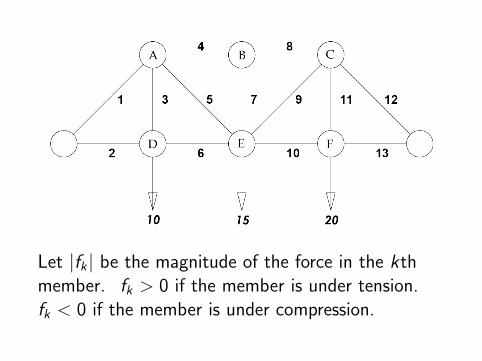
Let |fk | be the magnitude of the force in the kthmember. fk > 0 if the member is under tension.fk < 0 if the member is under compression.

Static equilibrium at the joint A:
horizontal projection: − 1√2f1 + f4 + 1√
2f5 = 0
vertical projection: − 1√2f1 − f3 − 1√
2f5 = 0
Static equilibrium at the joint B:
horizontal projection: −f4 + f8 = 0
vertical projection: −f7 = 0
Static equilibrium at the joint C:
horizontal projection: −f8 − 1√2f9 + 1√
2f12 = 0
vertical projection: − 1√2f9 − f11 − 1√
2f12 = 0

Static equilibrium at the joint D:
horizontal projection: −f2 + f6 = 0
vertical projection: f3 − 10 = 0
Static equilibrium at the joint E:
horizontal projection: − 1√2f5 − f6 + 1√
2f9 + f10 = 0
vertical projection: 1√2f5 + f7 + 1√
2f9 − 15 = 0
Static equilibrium at the joint F:
horizontal projection: −f10 + f13 = 0
vertical projection: f11 − 20 = 0

− 1√2f1 + f4 + 1√
2f5 = 0
− 1√2f1 − f3 − 1√
2f5 = 0
−f4 + f8 = 0
−f7 = 0
−f8 − 1√2f9 + 1√
2f12 = 0
− 1√2f9 − f11 − 1√
2f12 = 0
−f2 + f6 = 0
f3 = 10
− 1√2f5 − f6 + 1√
2f9 + f10 = 0
1√2f5 + f7 + 1√
2f9 = 15
−f10 + f13 = 0
f11 = 20