MATH 217C NOTES

ARUN DEBRAY

AUGUST 21, 2015

These notes were taken in Stanford’s Math 217c class in Winter 2015, taught by Eleny Ionel. I live-TEXed them using vim,

and as such there may be typos; please send questions, comments, complaints, and corrections to a.debray@math.utexas.edu.

Thanks to Ikshu Neithalath for finding a few errors.

Contents

1. Introduction, Complex Manifolds and Holomorphic Maps: 1/6/15 12. Complex Manifolds from Two Different Perspectives: 1/8/15 43. Tensor Calculus for Complex Manifolds: 1/13/15 74. Dolbeault Cohomology and Holomorphic Vector Bundles: 1/15/15 95. Holomorphic Vector Bundles and More Dolbeault Cohomology: 1/20/15 126. Hermitian Bundles and Connections: 1/22/15 147. Kahler Metrics: 1/27/15 168. Curvature on Kahler Manifolds: 1/29/15 199. Hodge Theory: 2/3/15 2110. The Hard Lefschetz Theorem: 2/5/15 2411. Line Bundles and Chern Classes: 2/10/15 2412. 2/12/15 2613. Sheaves and Cech Cohomology: 2/17/15 2614. 2/19/15 2915. Special Holonomy and Kahler-Einstein Metrics: 2/24/15 29

“A differential geometer whose work often uses the simplifications obtained by considering thecomplex domain explained to me that the additional structure of complex manifolds makes them moreinteresting, just as two sexes are more interesting than one, but various aspects of this argument areopen to debate.” – Michael Spivak

1. Introduction, Complex Manifolds and Holomorphic Maps: 1/6/15

The audience of the class has quite a varied background; some days, some people will be quite bored and others willfind it quite difficult. We’ll try to stay at an elementary level; this is an introductory course in complex differentialgeometry, supposed to be a second-year graduate-level course. In particular, this is not a topics course.

We’re going to be most interested in complex manifolds and related structures, and we’ll approach them withdifferential geometry and complex analysis. There’s another approach which uses algebra, which we’re not going totalk about as much. We’re not going to follow any textbook particularly closely; here are the course topics (possiblyout of order).

• Complex structures, almost complex structures, and integrability.• Hermitian and Kahler metrics.• Connections.• Complex vector bundles, holomorphic vector bundles, connections and curvature.• Chern classes and Chern-Weil theory.• Many examples; in particular, the physicists will be interested in Calabi-Yau manifolds and Kahler-Einstein

metrics and the relationship with physics.• Cohomology theories: Hodge theory and Dolbeault cohomology.• Vanishing theorems.• Deformation theory and Kodaira-Spencer theory.

1

Since this is a second-year class, there will be no final and no midterm, but there will be homeworks; as usual, thebest way to understand the material is to work through the examples.

We mentioned that there are the two analytic or algebraic approaches to complex differential geometry; the bestresults follow from combining the two. Here are some references for the class, recommended but not followed exactly.

• Moroianu, Lectures on Kahler Geometry. These lecture notes are short and to the point, and thus serve as auseful introduction. The first six lectures cover elementary differential geometry, which is a useful reference,since it will be assumed in this class.

• Huybrechts, Complex Geometry. This is a more detailed reference, and uses more complex analysis, and alittle algebra. This is a cleaned-up version of Griffiths’ and Harris’ Principles of Algebraic Geometry (whichis nonetheless still mostly analytic).

• Voisin, Hodge Theory and Complex Algebraic Geometry: Volume I. This is less relevant to the course, but itsalgebraic approach is useful and interesting.

• Demailly, Complex Analytic and Differential Geometry. This is also less relevant to the course; it mixes theanalytic and algebraic approaches.

Now, let us enter the world of mathematics.In this class, we want to study complex manifolds; we’ll define them precisely in a moment, but one can think

of these as spaces covered by charts, where each chart locally looks like Cn, and the change-of-charts maps areholomorphic, i.e. complex differentiable; the linearization is complex linear. Complex manifolds are special cases ofreal manifolds, but there are real manifolds which cannot be complexified.

Kahler manifolds are a special class of complex manifolds; not every complex manifold is Kahler. Cn and CPn areKahler, as are complex submanifolds of CPn and Calabi-Yau manifolds. These will have relatively nice properties.

A real manifold may have several complex structures (which will play a role in deformation theory), and similarlya complex manifold may have several Kahler structures.

This class will assume some knowledge of real differential geometry, and the study of real manifolds. One studiesa real manifold by adding structure, e.g. a metric (turning it into a Riemannian manifold). Adding a metric isn’tcanonical, but forgetting it is. Similarly, we’ll view a complex manifold as a complex structure on a real manifold,and we can add additional struture, such as a Hermitian metric (where the inner product is Hermitian), producingwhat is called a Hermitian manifold. Like a Riemannian metric, there is always such a metric and generally manychoices, and forgetting the complex structure, one obtains a Riemannian metric. Kahler metrics (and their associatedKahler manifolds) are special cases of Hermitian manifolds.

We’ll develop tools to prove our main results, mostly from differential geometry (connections, bundles, curvature),but also a little from algebraic topology (typically cohomology). The idea is that a complex structure places restrictionson the underlying topology of the manifold.

We will have three types of main results.

(1) The Hodge and Lefschetz theorems impose strong restrictions on the cohomology of Kahler manifolds, and inparticular implies that there are complex manifolds that do not admit a Kahler structure.

(2) Vanishing results, e.g. the Kodaira vanishing theorem and its applications, such as Kodaira embedding.These results can also be stated in terms of cohomology (specifically, H0 vanishes). Intuitively, this resultstates that if a complex line bundle has negative curvature, then it has no nontrivial holomorphic sections;then, the Kodaira vanishing theorem states that under the assumption of positive curvature, all of the highercohomology groups Hq(M,E) on the manifold M and line bundle E vanish (i.e. q > 1).

With the Riemann-Roch theorem (which itself is a special case of an index theorem), we can reframe thisas a criterion for nice Kahler manifold to be embedded in CPN for some large N . This is quite a surprise,because in the complex case things are very different from Rn: there are no partitions of unity and no compactcomplex submanifolds of Cn (other than a point), which ultimately follows from Liouville’s theorem.

(3) In deformation theory, one asks how many differentiable complex structures there are on a given smoothmanifold. This is a bit of a hopeless question, but we can ask the infinitesimal version: given a complexstructure, how any infinitesimal deformations are there? These end up being once again governed by anothercohomology group, and in particular, complex structures come in finite-dimensional families, unlike, say,Riemannian structures. However, not all of these first-order variations are integrable (which yields globalstructures from local ones), but higher-order cohomology groups dictate whether a global structure can beobtained.

A lot of questions concerning complex structure are difficult, and some are even open. For example, does S6 admit acomplex structure? We know it’s not Kahler, but otherwise this is an open question. Note that S6 is compact, butthere’s a possibility that it has a complex structure that can’t be embeddied in Cn.

2

Holomorphic maps and complex manifolds. Since everyone in the class has seen single-variable complex analysis,we can use it to move to several complex variables.

Definition. A domain will refer to an open, connected subset of Cn.

For the time being, U will always refer to a domain.

Definition. A function f : U → Cm is holomorphic if it is complex differentiable, i.e. df is complex linear.

We’ll clarify what complex linear means in just a little bit.This is equivalent to any of the following:

• f satisfies the Cauchy-Riemann equations.• ∂f = 0.• f is analytic.• f has a continuous complex differential.

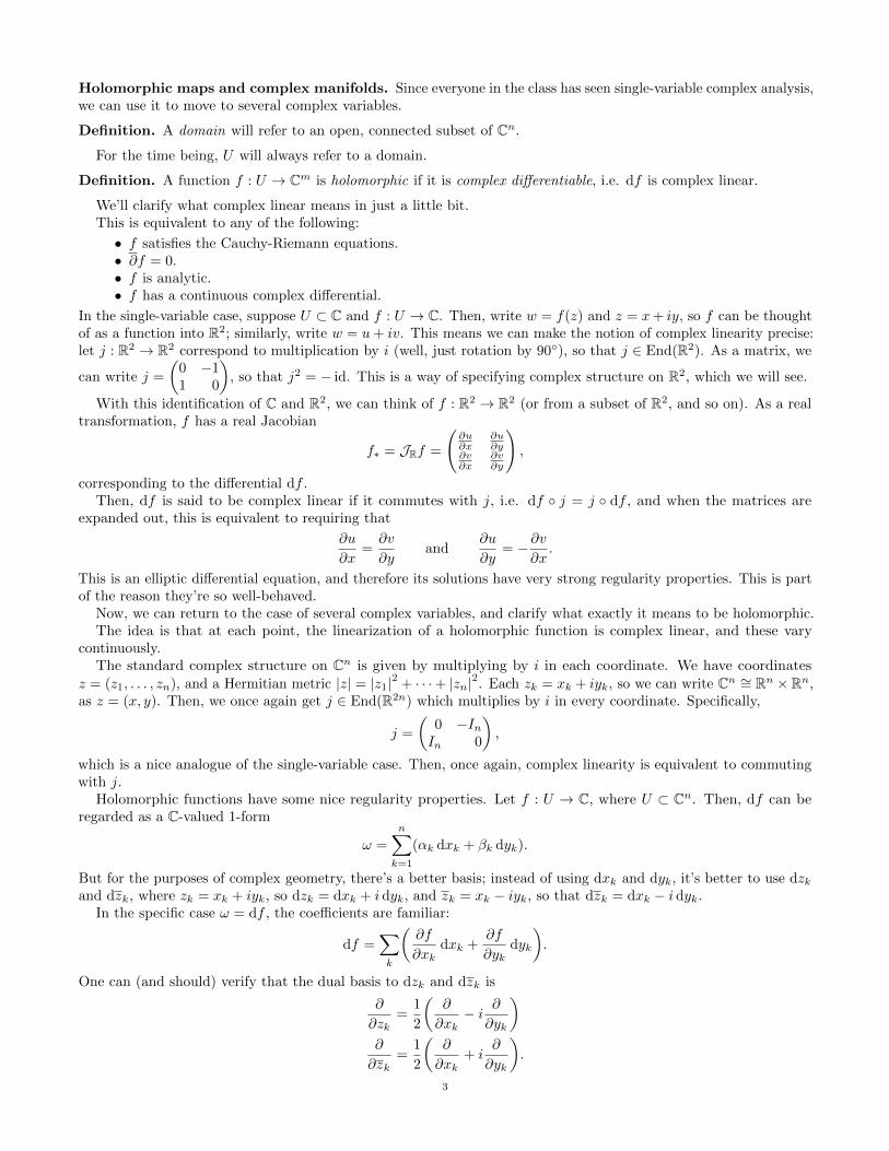
In the single-variable case, suppose U ⊂ C and f : U → C. Then, write w = f(z) and z = x+ iy, so f can be thoughtof as a function into R2; similarly, write w = u+ iv. This means we can make the notion of complex linearity precise:let j : R2 → R2 correspond to multiplication by i (well, just rotation by 90), so that j ∈ End(R2). As a matrix, we

can write j =

(0 −11 0

), so that j2 = − id. This is a way of specifying complex structure on R2, which we will see.

With this identification of C and R2, we can think of f : R2 → R2 (or from a subset of R2, and so on). As a realtransformation, f has a real Jacobian

f∗ = JRf =

(∂u∂x

∂u∂y

∂v∂x

∂v∂y

),

corresponding to the differential df .Then, df is said to be complex linear if it commutes with j, i.e. df j = j df , and when the matrices are

expanded out, this is equivalent to requiring that

∂u

∂x=∂v

∂yand

∂u

∂y= −∂v

∂x.

This is an elliptic differential equation, and therefore its solutions have very strong regularity properties. This is partof the reason they’re so well-behaved.

Now, we can return to the case of several complex variables, and clarify what exactly it means to be holomorphic.The idea is that at each point, the linearization of a holomorphic function is complex linear, and these vary

continuously.The standard complex structure on Cn is given by multiplying by i in each coordinate. We have coordinates

z = (z1, . . . , zn), and a Hermitian metric |z| = |z1|2 + · · ·+ |zn|2. Each zk = xk + iyk, so we can write Cn ∼= Rn ×Rn,as z = (x, y). Then, we once again get j ∈ End(R2n) which multiplies by i in every coordinate. Specifically,

j =

(0 −InIn 0

),

which is a nice analogue of the single-variable case. Then, once again, complex linearity is equivalent to commutingwith j.

Holomorphic functions have some nice regularity properties. Let f : U → C, where U ⊂ Cn. Then, df can beregarded as a C-valued 1-form

ω =

n∑k=1

(αk dxk + βk dyk).

But for the purposes of complex geometry, there’s a better basis; instead of using dxk and dyk, it’s better to use dzkand dzk, where zk = xk + iyk, so dzk = dxk + i dyk, and zk = xk − iyk, so that dzk = dxk − i dyk.

In the specific case ω = df , the coefficients are familiar:

df =∑k

(∂f

∂xkdxk +

∂f

∂ykdyk

).

One can (and should) verify that the dual basis to dzk and dzk is

∂

∂zk=

1

2

(∂

∂xk− i ∂

∂yk

)∂

∂zk=

1

2

(∂

∂xk+ i

∂

∂yk

).

3

Mind the sign change.Then, we have operators ∂ and ∂, defined as

∂f =∑k

∂f

∂zkdzk

∂f =∑k

∂f

∂zkdzk.

Hence, df = ∂f + ∂f , and f is holomorphic iff ∂f = 0.In this new basis, j is considerably easier to write down.Here are some useful properties of holomorphic functions. Most come from one variable, and many but not all

extend to several variables; there are a few properties which are only true in several complex variables.

Theorem 1.1 (Cauchy integral formula). Let U ⊆ C be a ball (this can be made more general), f : U → C beholomorphic on U so that it extends continuously to U . Then, for any z0 ∈ U ,

f(z0) =1

2πi

∫∂U

f(z) dz

z − z0.

From a differential-geometric perspective, this states that

α =f(z) dz

z − z0is a closed one-form on U \ z0 (which you can check by computing dα = 0), so this is essentially a corollary ofStokes’ theorem. This also relies on the calculation that

1

2πi

∫|z−z0|=ε

f(z) dz

z − z0ε→0−→ f(z0).

This generalizes to several complex variables thanks to Fubini’s theorem. Let U be a polydisc (i.e. a product of discs),and f : U → Cn be holomorphic on U and extend continuously to U . Then, the iterated integral satisfies

f(w) =1

(2πi)n

∫f(w) dw

(w1 − z1) · · · (wn − zn),

where dw = dw1 ∧ · · · ∧ dwn, where the integral is taken over the product of the boundaries.Regarding the integrand as a power series, we can see the following.

Theorem 1.2 (Osgood). A holomorphic function of several variables is complex analytic (i.e. given by a complexpower series).

2. Complex Manifolds from Two Different Perspectives: 1/8/15

The two perspectives will be thinking of complex manifolds as integrable almost complex manifolds (linear algebraic)and a more complex-analytic perspective.

A complex manifold is just like a real manifold, except that the charts are subsets of Cn and the transition mapsare holomorphic.

Definition. A n-dimensional complex manifold M is a smooth manifold on which there exists a collection of charts(Uα, ϕα) covering M , where each Uα ⊂ M is open and ϕα : Uα → Cn has open image. Furthermore, if α and βgive two charts, then the transition maps ϕ−1β ϕα are holomorphic on the overlaps.

The charts are called holomorphic charts, and the coordinates they induce are called holomorphic coordinates.

Note. In this class, we will require all manifolds to be Hausdorff, and have a countable topological basis.

Note. Just as the same topological manifold may admit many smooth structures, a smooth manifold can admitdifferent complex structures; this will be useful in deformation theory.

Definition. f : M → C is holomorphic if f ϕ−1α is holomorphic for all holomorphic charts. Similarly, f : M → N isholomorphic if it is holomorphic as a map Cm → Cn on each chart.

One can check that these are well-defined notions, no matter which set of charts one uses.

Note. There are no nonconstant holomorphic functions on a compact, connected, complex manifold, which is just acorollary of the maximum modulus principle (in several variables, which follows from the single-variable statement, bychecking each coordinate). This is one of the huge differences between complex geometry and real geometry.

4

Definition. f : M → N is a biholomorphism if it is a holomorphic bijection and f−1 is also holomorphic.

This is the notion of equivalence in complex geometry, akin to a diffeomorphism in differential topology. If M andN are biholomorphic, one writes M ' N .

Another interesting fact is that the size of the charts matters; Liouville’s theorem (in one variable) implies thatC 6' D.

Note. More worryingly, when n ≥ 2, the unit ball (‖z‖ < 1) is not holomorphic to the polydisc (the product of n discs,or |z1| < 1, . . . , |zn| < 1). The proof is not that easy, but ultimately it’s because they have different automorphismgroups; the automorphism group of the unit ball contains U(n), but that of the polydisc is abelian (once the originis fixed). In particular, the Riemann mapping theorem does not extend to several variables (though the maximummodulus principle and analytic continuation both extend).

This is why we will prefer polydiscs to balls for bases; it allows us more naturally to do complex geometry in eachvariable.

Example 2.1.

(1) Cn is a complex manifold, with only one chart. More generally, any finite-dimensional complex vector spaceV is a complex manifold (which will be useful when there’s no natural basis). In complex geometry, this iscalled affine space.

(2) Similarly, any open subset of Cn is also a manifold.(3) More nontrivially, we can make tori : consider a lattice Λ in Cn, e.g. Λ = Z2n, which can be thought of as n

linearly independent vectors (over R) and then integer linear combinations of them. Then, Cn/Λ is a complexmanifold, and is diffeomorphic to T 2n = S1 × · · · × S1︸ ︷︷ ︸

2n times

.

For example, if n = 1 and Λ = Z ⊕ τZ, for τ ∈ C \ R, the quotient is an elliptic curve. Not all ellipticcurves are biholomorphic, and therefore not all tori of a given dimension are. Eτ ' Eτ ′ iff τ ′ = Aτ for anA ∈ SL(2,Z), i.e. the two lattices can be taken into each other by a linear transformation (which is where thespecial linear group comes from). Nonetheless, all tori of the same dimension are diffeomorphic.

(4) We also have complex projective space CPn, which is geometrically the space of complex lines in Cn+1. It’shard to put a complex structure on it from this perspective, so it’s easier to think of it algebraically, asCPn = (Cn+1 \0)/C∗, where C∗ = C\0 and a λ ∈ C∗ acts on Cn+1 \0 by (z0, . . . , zn) 7→ (λz0, . . . , λzn).Thus, points on the same line through the origin are identified, so this is really the same thing.

Once we quotient out, keep the same coordinates: [z] = [z0, . . . , zn], where scaling factors are ignored (andbrackets are used so we don’t forget this). These are sometimes known as homogeneous coordinates.

To get charts, take

Ui = [z0, . . . , zn] ∈ CPn | zi 6= 0and ϕi : Ui → Cn given by

ϕi([z0, . . . , zn]) =

(z0zi, . . . ,

zi−1zi

,zi+1

zi, . . . ,

znzi

).

CPn \ Ui is Hi = [z0, . . . , zn] | zi = 0, which is called the hyperplane at infinity in the ith coordinate.Hi ' CPn−1, so Hi is closed, and therefore Ui is open.

To see that ϕi is a bijection, its inverse is just (w0, . . . , wn) 7→ [w0, . . . , wi−1, 1, wi+1, . . . , wn]. It’s not toohard to check that the transition maps are holomorphic (because the product of holomorphic functions isholomorphic, and the quotient is too, whenever the denominator doesn’t vanish, just as in the single-variablecase).

A special case of this is the Riemann sphere CP1 = S2. The two hyperplanes at infinity are the north andsouth poles.

The process of obtaining CPn from Cn+1 is called projectivizing ; one can do this to any (finite-dimensional)complex vector space V to get P(V ) = (V \ 0)/C∗. This is of course biholomorphic to CPn, but there mightnot be a natural biholomorphism.

(5) The complex Grassmanian of k-dimensional complex planes in Cn is also a complex manifold; when k = 1 ork = n− 1, this is the same as CPn−1.

(6) The Hopf manifold is the quotient of Cn \ 0 by Z acting as follows: fix a λ > 1 (the topology is independentof the choice of λ) and for k ∈ Z, k ∗ (z1, . . . , zn) = (λkz1, . . . , λ

kzn). The resulting quotient is a complexmanifold diffeomorphic to S1 × S2n−1, and will be important because when n ≥ 2, it will provide an exampleof a complex manifold that cannot admit a Kahler structure (for topological reasons). When n = 1, one getsa torus which is an elliptic curve, and it’s possible to explicitly write down which lattice it corresponds to.

5

(7) To produce more examples, one can talk about complex submanifolds in precisely the same way as one wouldtalk about real submanifolds. N is a k-dimensional complex submanifold of an n-dimensional manifold M ifthere exists a collection of holomorphic charts on M covering N such that the image of N under the chartmaps is linear (specifically, Cn−k).

This definition is motivated by the inverse function theorem; there are plenty of other definitions, butfortunately they’re all equivalent.

Now, we can define lots of complex submanifolds of Cn or CPn; for example, if f : Cn → C is holomorphic,then the zero locus of f , i.e. Z(f) = f−1(0), is a complex manifold by the implicit function theorem. Usefulexamples of this include polynomials; if f is cubic, then Sard’s theorem is another way to show that forgeneric coefficients, the zero locus is smooth (i.e. 0 is a regular value) and therefore is a complex manifold.

If f : Cn+1 → C is a homogeneous polynomial of degree k, i.e. f(λz0, . . . , λzn) = λkf(z0, . . . , zn), e.g.f(z0, z1) = z30 + z0z

21 + z31 , then Z(f) ⊂ Cn+1, and if 0 is a regular value (which is not always true), then the

homogeneity guarantees that Z(f) descends as a submanifold of CPn. Now we can talk about varieties andall that.

(8) Another large class is the complex Lie groups, groups with a complex manifold structure such that multiplicationand inversion (equivalently (x, y) 7→ x−1y) are holomorphic. For example GL(n,C) is a complex Lie group,but U(n) is not (for example, U(1) = S1 isn’t even-dimensional!), ultimately because all compact, complexLie groups are abelian (because the adjoint map is holomorphic and bounded, and therefore constant), andthen (a bit harder to show) one can show they’re all tori.

A lot of these examples were quotients; other examples exist, but they’re sometimes harder to construct.

Another Perspective. For the purposes of deformation theory, there’s a different, equivalent definition of a complexmanifold, and it will be useful for some other cases, too. This will be more linear-algebraic, involving differentialcalculus or tensor calculus on complex manifolds. The idea is to take the linear-algebraic notion of an almost complexstructure and then require integrability. In the process of defining this, we can also discuss the Dolbeault cohomology.

If M is a complex manifold, one would expect TM to be a complex vector bundle, and that’s what we’re going tosee.

Definition. An almost complex structure on a real manifold M is a vector bundle endomorphism J ∈ End(TM )such that J 2 = − id.

Note. J makes TM into a complex vector bundle, as (a+ ib) ·X = aX + bJX for all a, b ∈ R and X ∈ TM . Thus,J is really just multiplication by i.

We’ll define complex vector bundles later, but the general idea is that each fiber is a complex vector space and thetrivialization functions can be chosen to be complex linear.

Lemma 2.2. If M is a complex manifold, then multiplication by i in each holomorphic coordinate chart induces awell-defined almost complex structure on TM .

Proof. We’ll differentiate multiplication by i and see what happens, and then prove its independence of choice ofholomorphic chart.

Let’s pick holomorphic coordinates (z1, . . . , zn), and decompose them into zk = xk + iyk, so we have basis vectors∂∂xk

and ∂∂yk

for the tangent space. Then, define J as last lecture, i.e. J(

∂∂xk

)= ∂

∂ykand J

(∂∂yk

)= − ∂

∂xk, and

write z = (x, y), so Cn = Rn × Rn. Then, J is the same matrix as last time, and J 2 = − id (as a matrix or justby the action on the basis), and it’s independent of a change of coordinates, because a change of coordinates ψ isholomorphic, i.e. it commutes with J .

For the rest of this lecture, assume J is an almost complex structure. A lot of the linear algebra we want stillworks for almost complex structures, though not all of it. Since J 2 = − id, then its eigenvalues are ±i. After wecomplexify, it can even be diagonalized.

Consider the complexified tangent space TCM = TM ⊗R C. Tensoring with C is what is meant by complexifying.TCM is a complex vector space of dimension n.

Lemma 2.3. Let T 1,0(M) (resp. T 0,1(M)) denote the i (resp. −i) eigenbundle (i.e. eigenspace at each fiber) of J .Then:

(1) TCM = T 1,0M ⊕ T 0,1M .(2) T 1,0M = X − iJX | X ∈ TM .(3) T 0,1M = X + iJX | X ∈ TM .

6

Proof. Regard Z ∈ TCM as Z = X+iY for X,Y ∈ TM . Then, define T 1,0M and T 0,1M as in (2) and (3), respectively;one can check that for all Z ∈ T 1,0M , JZ = iZ, because J (X − iJX) = JX − iJ 2X = JX + iX = i(X − iJX).Then, the decomposition (1) is immediate, because any X satisfies 2X = (X − iJX) + (X + iJX).

Next time, we’ll talk about the integrability condition.

3. Tensor Calculus for Complex Manifolds: 1/13/15

Last time, we started talking about tensor calculus on the tangent bundle, but we can place it in the more generalsetting of complex vector spaces to make it useful in more places.

Definition. A complex vector space is a real vector space V together with a real linear J : V → V such thatJ 2 = − id.

This gives it the structure of a vector space over C, but this alternate definition is useful as well.

Definition. The complex conjugage of a complex vector space (V,J ) is V = (V,−J ).

We can complexify V by taking V ⊗R C; it’s already complex, but now we have the structure induced by C, so wecan take its i-eigenspace V 1,0 and its −i-eigenspace V 0,1; thus, V ⊗R C = V 1,0 ⊕ V 0,1. As complex vector spaces,V 1,0 = V 0,1 ∼= (V,J ) (where V 1,0 has complex structure given by multiplication by i).

This extends to the dual V ∗ and exterior powers in the same way.

Note. If V is already a complex vector space, then V ⊗R C = V ⊕ V . (It also has a quaternionic structure, but that’sless important.)

Now, we can apply this linear algebra to manifolds. Assume (M,J ) is an almost complex manifold; then, we canapply the above to its tangent space: TM ⊗R C = T 1,0M ⊕ T 0,1M . To use forms, we’ll look at the cotangent bundleT ∗M = Λ1M . We can complexify it, to obtain Λ1

CM = Λ1,0 ⊕ Λ0,1.

Definition. If M is a complex manifold with local holomorphic coordinates (z1, . . . , zn). T 1,0M is also denoted

τM , and is called the holomorphic tangent space; its local basis is

∂∂zk

. Similarly, T 0,1M = τM is called the

anti-holomorphic tangent space, and has a local basis

∂∂zk

.

We want the dual structure to factor through the direct sum, so let

Λ1,0 = ω ∈ Λ1CM | ω(X) = 0 for all X ∈ T 0,1M,

and Λ0,1 is defined similarly (with T 1,0 in place of T 0,1). Thus, Λ1,0 = η− iη J | η ∈ Λ1M, and Λ0,1 = η+ iη J |η ∈ Λ1M.

We can extend this to (p, q)-forms by using the fact that

Λk(E ⊕ F ) =

k⊕j=1

ΛjE ⊗ Λk−jF.

Thus, we just wedge p things in Λ1,0 and q things in Λ0,1 together to get a basis, i.e. Λp,qM = Λp(Λ1,0M)⊗Λq(Λ0,1M).Then, ΛkCM =

⊕p+q=k Λp,qM .

Definition. Denote by Ap,q the space of smooth (p, q)-forms on M . That is, this is the space of sections Γ(Λp,q).

In differential geometry, this space of sections is usually denoted Ω, but this will be used for holomorphic sectionslater.

Again, if M is a complex manifold, we have some nice bases.

• A basis for Λ1,0 is given by dzk = dxk + i dyk.• Similarly, a basis for Λ0,1 is given by dzk = dxk − idyk.• If η ∈ Ap,q (i.e. η is a (p, q)-form), then in local coordinates

η =∑I,J

ηIJ dzI ∧ dzJ ,

where dzi = dzi1 ∧ · · · ∧ dzip and dzJ = dzj1 ∧ · · · ∧ dzjq , where i1 < · · · < ip and j1 < · · · < jq.1 The

coefficients ηIJ are smooth functions.

1Sometimes, the notation ηIJ is used. This has no content, but is an interesting reminder, and sometimes is useful for keeping track of

things.

7

All of this linear algebra works for almost complex manifolds, so let’s talk about integrability, which will make thedifference.

Definition. Assume (M,J ) is an almost complex structure. Then, the Nijenhuis2 tensor is

NJ (X,Y ) = [X,Y ] + J [JX,Y ] + J [X,J Y ]− [JX,J Y ].

Here, X,Y ∈ TM , though we can complexify.

Exercise 3.1. Check that NJ is actually a tensor.

The Nijenhuis tensor’s signs aren’t arbitrary, and we’ll see how to derive them,

Proposition 3.2. If J comes from a complex structure on M , then NJ = 0.

This can be proven by checking for X,Y ∈

∂∂xk

, ∂∂yk

.

The converse is also true, which is the harder direction.

Theorem 3.3 (Newlander-Nirenberg Integrability Theorem). If NJ = 0, then J comes from a complex structure onM .

Proof sketch. If NJ = 0 and J is real analytic, then the Frobenius integrability theorem tells us that J is integrable.But the hard part is the regularity result: it’s beautiful, but hard to show that NJ = 0 induces a differential equationwhich leads J to be real analytic.

Proposition 3.4. Assume J is an almost complex structure on a smooth manifold M . Then, the following areequivalent:

(1) J comes from a complex structure on M .(2) NJ = 0.(3) T 1,0M is formally integrable, i.e. for any Z,W ∈ T 1,0M , [Z,W ] ∈ T 1,0M .(4) T 0,1is formally integrable.(5) d(A1,0) ⊆ A2,0 ⊕A1,1 (i.e. there’s no (0, 2)-component).(6) d(Ap,q) ⊆ Ap+1,q ⊕Ap,q+1.

When we define ∂, we will see that this is also equivalent to ∂2

= 0.

Proof sketch. We’re only going to show the easier parts, as we saw in the proof sketch of Theorem 3.3 it can get quitedifficult.

To see why (2) ⇐⇒ (3), suppose Z ∈ T 1,0M , so that Z = X − iJX for X ∈ TM . If we take X,Y to be localvector fields on M , then we can regard them as vector fields in T 1,0M ; then, let Z = X − iJX and W = Y − iJX,so one can check that [Z,W ] = NJ (X,Y ) + iJNJ (X,Y ).

To see why (3) ⇐⇒ (5), take a (1, 0)-form ω, so that ω(Z) = 0 for Z ∈ T 0,1M . Thus, dω has no (0, 2)-part. Thisis equivalent to showing that dω(Z,W ) = 0 for all Z,W ∈ T 0,1M . But we can expand this out to

dω(Z,W ) = Z · ω(W )−W · ω(Z)− ω[Z,W ],

but the condition given shows ω(Z) = ω(W ) = 0, so therefore dω has no (0, 2)-part iff the Lie bracket [Z,W ] ∈ T 0,1Mfor all Z,W ∈ T 0,1M , which is (4), and by complex conjugation, we get (3). Then, by the Leibniz rule, this can beextended to (6), and the other direction is immediate.

What’s left is the equivalences of (1), (2), and (3), which is more or less the content of Theorem 3.3 and uses theFrobenius integrability theorem.

Now, let’s use this.

Proposition 3.5. Any almost complex structure on a real, orientable 2-manifold is integrable.

Proof. This is by dimensionality: NJ (X,X) = 0 and NJ (X,JX) = 0, so that’s all we need for a basis.

Note. An almost complex structure is a topological condition (which we’ll see because it involves cohomology), andtherefore the only spheres that admit almost complex structures are S2 and S6.

On S6, one can explicitly create a nonintegrable almost complex structure by considering it to be the unit spherein R7, which can be regarded as the imaginary part of the octonions O (sometimes this is called the Cayley numbers).Then, there is a definition of a cross product p× v ⊥ p if v ⊥ p, and then Jp(v) = p× v. Calabi showed this isn’tintegrable; there may be others which could be integrable, but this is still open.

2Prononced “nigh-house.”

8

Condition (2) of Proposition 3.4 implies that if G is a complex Lie group, then its Lie algebra TeG is also a complexLie algebra.

One would expect (and it’s true) that if M is a compact complex manifold, then Aut(M), the set of biholomorphicfunctions M → M , is a Lie group. Its Lie algebra is the space of infinitesimal automorphisms of M , i.e. flows of“holomorphic” vector fields. We haven’t defined these precisely; that’s all right.

Definition. If M is a complex manifold, then a holomorphic vector field on M is a vector field = X − iJX ∈ T 1,0M(i.e. X is real) such that the flow of X consists of holomorphic maps, i.e. LXJ = 0.

Later, we’ll see that these are equivalent to holomorphic sections of τM , the holomorphic vector bundle. For now,if (z1, . . . , zk) are holomorphic coordinates on M , then

Z =∑k

ak(z1, . . . , zn)∂

∂zk,

where the ak are holomorphic functions. Again, to show all of these things, there’s a lot of linear algebra.

Dolbeault cohomology. Suppose M is a complex manifold, so that condition (6) of Proposition 3.4 implies that wehave a map d : Ap,q → Ap+1,q⊕Ap,q+1. Thus, we can define ∂ = πp−1,q d and ∂ = πp,q+1d. Thus, ∂ : Ap,1 → Ap+1,q

and ∂ : Ap,q → Ap,q+1.These are both differential operators (i.e. C-linear and satisfying the Leibniz rule, which one can check); furthermore

∂2 = ∂2

= 0, and they anti-commute, as ∂∂ + ∂∂ = 0. This can be checked because d2 = 0, and then expanding out.Now, we have something called the Hodge complex :

A0,0

∂

∂

A1,0

∂

∂

A0,1

∂

∂

A2,0 A1,1 A0,2

and so on.

Definition. The (p, q) Dolbeault cohomology group Hp,q(M) is the (co)homology of Ap,•∂→ Ap,•+1. That is, it is the

∂-closed (p, q)-forms on M mod the ∂-exact (p, q)-forms on M .

4. Dolbeault Cohomology and Holomorphic Vector Bundles: 1/15/15

“I don’t know why, but I always forget the 1/(2πi) term in the Cauchy integral formula!”

Recall that we had a chain complex Ap,0∂→ Ap,1

∂→ · · · , and the Dolbealut cohomology group Hp,q(M) is the qth

homology group of the complex.

Definition. The Hodge numbers hp,q(M) of the manifold are given by the ranks of the respective Dolbeaultcohomology groups.

It’s hard to calculate this from the definition, like any cohomology.

Example 4.1. However, one simple case is H0,0, because ∂-closed (0, 0)-forms are holomorphic functions, and thereare locally lots of them. In general, this could be infinite-dimensional, but if M is compact and connected, they’reglobally only constant, so H0,0(M) = C, which is nice.

Why do we care about this construction? One useful case is the existence of an invariant of the complex structure.Another useful thing is that it’s contravariant functorial: if f : M → N is a holomorphic map of complex manifolds,then there’s an induced f∗ : Hp,q(N)→ Hp,q(M), and it is a group homomorphism. But Dolbeault cohomology isalso useful in local deformation or obstruction theory, which can be useful for keeping track of obstructions to theexistence of a complex structure on a manifold.

Suppose one wants to solve the equation ∂β = α for a (p, q)-form α. If this were to have a solution, ∂α = 0 (i.e. αis ∂-closed), which can be checked locally. If there is no obstruction, then the equation has local solutions, but wemay not be able to patch them together to get a global solution on M . The global obstruction is governed by Hodgetheory, which says that if the cohomology class [α] ∈ Hp,q(M) vanishes, then we can do this.

There are two powerful tools to deal with this.9

• Sheaf theory adopts the approach of looking at locally holomorphic functions and forms, and spends timeworrying about how they patch together, which sheaves help with.• A more analytic approach is to use Sobolev spaces, which relax the holomoprhic condition, but require one to

worry about regularity.

Ideally, one could use both, but one may be more useful than the other in a given situation.This lemma is really due to Dolbeault, but has Poincare’s name on it for some reason.

Lemma 4.2 (∂-Poincare). Any ∂-closed (p, q)-form is locally ∂-exact.

As a corollary, if P is the polydisc, then Hp,q(P ) = 0 if q > 0.

Proof sketch. For the complete proof, see Huybrechts’ book, §1.3.We’ll use the polydisc for working locally, since analysis is easier in compact spaces.In one variable, assume g is smooth on the closed unit disc D; then, we want an f such that ∂f = g dz. We can

explicitly construct a solution:

f(z) =1

2πi

∫D

g(w)

w − zdw ∧ dw,

which is smooth on D and satisfies ∂f = g dz. This was a version of the Cauchy integral formula.Now, let’s talk about (0, 1)-forms in n variables; let

α =

K∑k=1

αj dzj ,

where K ≤ n. We’ll induct on K; since α is ∂-closed, then each αj is holomorphic in zK+1, . . . , zn.

One can integrate (made more precise in the book) the coefficient αK of dzK to get a β such that α − ∂β is alinear combination of dz1, . . . ,dzK−1, which is the necessary inductive step.

Then, we can generalize to (0, q)-forms from (0, 1)-forms. Let Ap,qK be space of (p, q)-forms that only involve

dz1, . . . , dzK . Then, filter A0,q by A0,qK ; one can show that if α ≡ 0 mod A0,q

K and α is ∂-closed, then one can find a β

such that α− ∂β ≡ 0 mod A0,qK−1.

Finally, generalizing yet further to (p, q)-forms is immediate from (0, q), since we’re merely adding dz terms.

For some purposes, it may be easier to have cohomology vanish on the open polydisc, which can be analyzedby exhausting it by closed polydiscs that approach it in the limit. Thus, there’s an extension problem, of taking asolution on one polydisc and extending it to a new solution on a larger polydisc which agrees (or mostly agrees) onthe smaller one.

Often in PDE theory, one considers a differential equation Df(x) = g(x) (where D is a differential operator).One way to solve this (intuitively, though it can be made precise) is to try to find a kernel k(x, y) which satisfiesDxk(x, y) = δx,y.3 Then, general principles tell us that

f(x) =

∫k(x, y)g(y) dy

is a solution of the differential equation. There are lots of important issues of convergence and making sense of this,but in the context where this works,

Dxf =

∫Dxk(x, y)g(y) dy =

∫δxyg(y) dy = g(x).

This applies to complex geometry: for us, D = ∂, and we want to solve ∂f = g. Our kernel was the Cauchy kernel

k(z, w) =dw

2πi(z − w).

Well, this is a one-form and not a function, and we’re secretly using a metric, and so on; this isn’t rigorous yet, but itcan be and will be; this is the intuition for later on.

Lemma 4.3 (Local ∂∂ Lemma). Let M be a complex manifold and ω be a real (1, 1)-form. Then, dω = 0 iff ω islocally of the form ω = i∂∂u for a (locally defined) real-valued function u.

In this case, u is called the potential.

3The δ function is not a function; it’s a distribution, of course, but the equation can be reformulated such that this is all right.

10

Proof. Suppose we know that ω = i∂∂u, and we want to show that it’s closed. Well, since ω is a (1, 1)-form,

dω = (∂ + ∂)(∂∂u) = ∂2∂u+ ∂∂∂u = −(∂)2∂u = 0,

because they anticommute.The other direction uses both the real and complex versions of the Poincare lemma; the real one is similar to the

complex one, but follows from Stokes’ theorem. Assume ω is d-closed, so that dω = 0. Then. by the real Poincarelemma, ω = dτ , for some real-valued 1-form τ . Then, thinking of τ as complex, we can uniquely decompose it asτ = τ1,0 + τ0,1; since τ is real, then τ0,1 = τ1,0 (which follows from the formula). Thus,

ω = dτ = ∂τ1,0︸ ︷︷ ︸(2,0)

+ ∂τ1,0 + ∂τ0,1︸ ︷︷ ︸(1,1)

+ ∂τ0,1︸ ︷︷ ︸(0,2)

.

But since this is a unique decomposition and ω is a (1, 1)-form, then ∂τ1,0 = 0, and similarly ∂τ0,1 = 0 too; thus,ω = ∂τ1,0 + ∂τ0,1.

By Lemma 4.2, τ0,1 = ∂f for a (local) complex-valued function f , and similarly the complex conjugate τ0,1 = ∂f .Thus,

ω = ∂τ1,0 + ∂τ0,1 = ∂∂f + ∂∂f

= 2∂∂(i Im(f)),

so let u = Im(f).

This proof follows a common approach of doing one thing from analysis followed by a bunch of linear algebra.We’ve talked about holomorphic functions, so it may also be useful to discuss holomorphic forms as well.

Definition. A holomorphic p-form is a (p, 0)-form ω such that ∂ω = 0.

Equivalently, ω is a holomorphic p-form iff it can be written as

ω =∑

ωI dzI ,

where the ωI are holomorphic functions. It turns out this will also be equivalent to ω being a section in a holomorphicvector bundle.

Note that if q 6= 0, a (p, q)-form α such that ∂α = 0 isn’t called holomorphic; we’l see why in a bit.

Holomorphic Vector Bundles. Intuitively, a holomorphic vector bundle is a complex vector bundle such that the

transition functions are holomorphic. Equivalently, it is a complex vector bundle with a ∂ operator such that ∂2

= 0.This last condition means that Dolbeault cohomology only makes sense over holomorphic vector bundles.

While one can define real and complex vector bundles over any topological space, holomorphic vector bundles canonly exist over complex manifolds.

Definition. Let M be a complex manifold. Then, a holomorphic vector bundle of rank r is a complex vector bundleπ : E →M such that the following hold.

• There exist holomorphic charts Uα covering M and holomorphic local trivializations, i.e. the following diagramcommutes.

π−1(Uα)

π

ψα // Uα × Cr

pr1Uα

• The transition functions gαβ : Uα ∩ Uβ → GL(n,C) are holomorphic. These are given as follows: going from

β → α, we have for x ∈M and e ∈ Cr, ψα ψ−1β (x, e) = (x, gαβ(x)e).

Example 4.4. Let M be a complex manifold.

• The trivial bundle M × Cr is of course a holomorphic vector bundle.• τM = T 1,0M (i.e. involving just ∂

∂z ) is a holomorphic vector bundle (but T 0,1M isn’t).

• Its dual (τM)∗ = Λ1,0M is holomorphic as well (which follows from its functorial properties); in complex andalgebraic geometry, this is often denoted ΩM , called the bundle of holomorphic one-forms.

• Ωp = Λp,0M , the space of (p, 0)-holomorphic forms.4

4These forms are sections of the bundle, so we should speak carefully, but they are frequently talked about as the same spaces. A

bundle can also be thought of as a sheaf of sections.

11

• The top power is a holomorphic line bundle, called the canonical line bundle. It has the special notationΩnM = Λn,0M . These are the analogues of volume forms, but in complex geometry.

Here’s why τM is holomorphic: choose local holomorphic coordinates (z1, . . . , zn) on M , so the local trivialization ofτM has as a basis ∂zk. We need to check that the change-of-coordinates and transition functions are holomorphic.

If z = z(w) is a change of holomorphic coordinates, then

∂

∂w`=∑k

∂zk∂w`

∂

∂zk,

with no extra terms because w is also holomorphic; thus, these coordinate changes are holomorphic.Similarly, a trivialization of ΩpM has basis dzII , where |I| = p for multi-indices I; one has to check that

dwK =∑|I|=p

∂wK∂zI

dzI

has holomorphic functions (which relates to the Jacobian of the change of coordinates z → w).

5. Holomorphic Vector Bundles and More Dolbeault Cohomology: 1/20/15

“You may have seen something like this [tautological line bundle] at IKEA.”

Recall that if M is a complex manifold, we have the holomorphic vector bundles, sections ΩM = τM∗ = Λ1,0M , whereτM = T 1,0M . Then, ΩpM = Λp,0M . Be careful, though; these are generally not Λp,q for q > 0.

A general principle here is tht most natural constructions on real vector bundles still work in the complex orholomorphic case. Here are some examples which stay holomorphic, where E and F are holomorphic vector bundles.

• The direct sum, E ⊕ F .• The tensor product E ⊗ F .• The dual E∗.• The exterior powers ΛkE, and as a special case, the determinant line bundle ΛrE, where r is the rank of E.• The pullback : if f : V →M is holomorphic and E →M is a vector bundle, then f∗ : V → N is a holomorphic

vector bundle. One useful example is that if V ⊂ N is a complex submanifold, the restriction of E|V isdefined as the pullback under inclusion i : V →M , and is holomorphic.5

Another useful fact about holomorphic vector bundles is that the total space is a complex manifold, with the projectionholomorphic.

Definition. Suppose V ⊂M is a complex submanifold. Let TM |V denote the restriction of TM to V ; then, we havea short exact sequence

0 // TVϕ // TM |V // NV // 0,

for a holomorphic bundle NV = coker(ϕ) called the normal bundle of V .

Keep in mind that while short exact sequences of complex vector bundles always split (i.e. if 0→ E → F → G→ 0is short exact, then F ∼= E ⊕G), this is not true for holomorphic bundles. For example, there’s a rank 2 bundle Eover an elliptic curve which fits into a short exact sequence 0→ C→ E → C→ 0 (where C denotes the trivial linebundle), but does not split. Since this sequence splits as a sequence of complex line bundles, we end up seeing thatthe same complex manifold may have nonisomorphic holomorphic structures.

Nonetheless, the determinant behaves well in short exact sequences: if 0→ E → F → G→ 0 is short exact, thendetF ∼= detE ⊗ detG as holomorphic line bundles. In particular, we have the adjunction formula det(TM |V ) ∼=det TV ⊗ detNV , which is used all the time.

Example 5.1. Consider the tautological line bundle τ over CPn. Geometrically, we want the fiber of τ at a line` ∈ CPn to be the line `. Algebraically, consider τ to be the total space τ = (`, u) ∈ CPn × Cn+1 | u ∈ `, whichcomes with the projection π onto the first factor.

This is a holomorphic line bundle: consider coordinate charts Ui on CPn, so zi 6= 0, which comes with the projectionπ onto the first factor.

This is a holomorphic line bundle: consider coordinate charts Ui on CPn, so zi 6= 0. The trivialization will beψi([z], u) = ([z], ui), which (you can check) plays well with transition functions gij([z])t = zi/zj , which is clearlyholomorphic.

When n = 1, CP1 is the Riemann sphere C ∪ ∞. Thus, we have two charts, z ∈ C and w = 1/z, whose overlapis C× (one ignores 0, the other ignores ∞). Thus, the transition functions are g(w)(t) = w−1t, for w ∈ C×.

5One can also pull back under the constant map, but the result is the trivial bundle.

12

This seems a little silly, but more interesting constructions, e.g. the canonical bundle or the tangent bundle, can bedescribed in terms of τ (e.g. T ∗M ∼= τ⊗2: the transitions of T ∗M are between dz and dw, so dw = d(1/z) = −1/z2 dz).

Remark. A complex or holomorphic vector bundle is determined by the transitions functions gαβ : Uα∩Uβ → GL(r,C)(where r is the rank of the vector bundle), such that gαβgβγ = gαγ on Uα ∩ Uβ ∩ Uγ , for all charts α, β, and γ. This

is known as the Cech cocycle condition, and relates to Cech cohomology, which we’ll discuss later.

Dolbeault Cohomology with Values in a Holomorphic Vector Bundle. Let E →M be a rank-r holomorphicvector bundle over an n-dimensional manifold. Choose a holomorphic trivialization (a local basis for the fiber)ekk=1,...,r, and let Λp,q(E) = Λp,qM ⊗ E. Then, we can define

∂E

(n∑k=1

ωk × ek

)=

k∑k=1

(∂ωk)⊗ ek,

where ωk are (p, q)-forms, i.e. in holomorphic coordinates (z1, . . . , zn),

ωk =∑I,J

ωIJk dzI dzJ .

Since ∂2

= 0, then ∂2

E = 0 as well, of course. And we can do some of the same stuff as before, taking smooth sectionsAp,q(E) of Λp,q(E) (since we can only differentiate sections, such as vector fields, rather than vectors themselves),and we get maps

Ap,0(E)∂E // Ap,1(E)

∂E // Ap,2(E)∂E // · · · (1)

This should look very familiar, and if E is the trivial line bundle we recover the Dolbeault cohomology from last time.

Definition. The Dolbeault cohomology of M with values in E Hp,q(M ;E) is the homology of the complex (1), i.e.the ∂E-closed (p, q)-forms with values in E modulo the ∂E-exact (p, q)-forms.

As a special case, H0,0(E) (sometimes Ω(E) or H0(M ;E); the latter notation comes from Cech cohomology) isthe sections σ of E which are holomorphic and satisfy ∂Eσ = 0, i.e.

σ =∑k

σk(z)⊗ ek

in a holomorphic frame, were the coefficients σk are holomorphic functions on M . Additionally, the tautological vectorbundle τ → CPn has no holomorphic sections (other than the zero section), which is a little bit of a chore to calculate.

There are more interesting examples, such as that of τ∗; one appears in the homework.

Remark. By the ∂-Poincare lemma (which still works just as well in this setup), over a polydisc (i.e. locally), (1)has trivial homology except in degree 0, where one gets Ω(E) = H0,0(M ;E). This is called an affine or an acyclicresolution, and leads to the following theorem.

Theorem 5.2 (Dolbeault). If Hq(M,F ) denotes the qth Cech cohomology with coefficients in F , then Hp,q(M ;E) =Hq(M,ΩpM ⊗ E).

This will be a little less mysterious once we actually define Cech cohomology.

Integrability of Complex Vector Bundles. The question is, when is a complex vector bundle (over a complexmanifold) a holomorphic vector bundle? The answer will be when there is an ∂E operating on smooth sections of E,i.e. ∂E : Λ0,0(E) → Λ0,1(E) that acts as a differential operator. That is, it satisfies the Leibniz rule: when ω is a(p, q)-form and σ is a section of E,

∂E(ω ⊗ σ) = (∂ω)⊗ σ + (−1)qω ⊗ ∂Eσ.

Furthermore, we require ∂2

E = 0.Once this exists, it can be extended using complex linearity and the Leibniz rule to ∂E : Λp,q(E)→ Λp,q+1(E).

Theorem 5.3. Assume E → M is a complex vector bundle over a complex manifold M . Then, a holomorphic

structure on E is uniquely determine by a C-linear differential operator ∂E : Λ0,0(E)→ Λ0,1(E) such that ∂2

E = 0.

This should be thought of as a linear version of Theorem 3.3, but for vector bundles.13

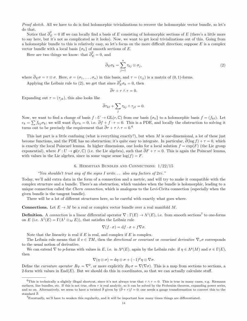
Proof sketch. All we have to do is find holomorphic trivializations to recover the holomorphic vector bundle, so let’sdo that.

Notice that ∂2

E = 0 iff we can locally find a basis of E consisting of holomorphic sections of E (there’s a little moreto say here, but it’s not as complicated as it looks). Now, we want to get local trivializations out of this. Going froma holomorphic bundle to this is relatively easy, so let’s focus on the more difficult direction; suppose E is a complexvector bundle with a local basis σk of smooth sections of E.

Here are two things we know: that ∂2

E = 0, and

∂Eσk =

n∑j=1

τkj ⊗ σj , (2)

where ∂Eσ = τ ⊗ σ. Here, σ = (σ1, . . . , σn) in this basis, and τ = (τij) is a matrix of (0, 1)-forms.

Applying the Leibniz rule to (2), we get that since ∂2

Eσk = 0, then

∂τ + τ ∧ τ = 0.

Expanding out τ = (τjk), this also looks like

∂τk` +∑j

τkj ∧ τj` = 0.

Now, we want to find a change of basis f : U → GL(r,C) from our basis σk to a holomorphic basis f = (fk`). Letek =

∑fkjσk; we will want ∂Eek = 0, i.e. ∂f + f · τ = 0. This is a PDE, and locally the obstruction to solving it

turns out to be precisely the requirement that ∂τ + τ ∧ τ = 0.6

This last part is a little confusing (what is everything exactly?), but when M is one-dimensional, a lot of these justbecome functions, and the PDE has no obstruction; it’s quite easy to integrate. In particular, ∂(log f) + τ = 0, whichis exactly the local Poincare lemma. In higher dimensions, one looks for a local solution f = exp(F ) (the Lie groupexponential), where F : U → gl(r,C) (i.e. the Lie algebra), such that ∂F + τ = 0. This is again the Poincare lemma,with values in the Lie algebra, since in some vague sense log(f) = F .

6. Hermitian Bundles and Connections: 1/22/15

“You shouldn’t trust any of the signs I write. . . also any factors of 2πi.”

Today, we’ll add extra data in the form of a connection and a metric, and will try to make it compatible with thecomplex structure and a bundle. There’s an obstruction, which vanishes when the bundle is holomorphic, leading to aunique connection called the Chern connection, which is analogous to the Levi-Civita connection (especially when thegiven bundle is the tangent bundle).

There will be a lot of different structures here, so be careful with exactly what goes where.

Connections. Let E →M be a real or complex vector bundle over a real manifold M .

Definition. A connection is a linear differential operator ∇ : Γ(E)→ Λ1(E), i.e. from smooth sections7 to one-formson E (i.e. Λ1(E) = Γ(Λ1 ⊗M E)), that satisfies the Leibniz rule

∇(f · σ) = df · σ + f∇σ.

Note that the linearity is real if E is real, and complex if E is complex.The Leibniz rule means that if v ∈ TM , then the directional or covariant or covariant derivative ∇vσ corresponds

to the usual notion of derivative.We can extend ∇ to p-forms with values in E, i.e. in Λp(E), again by the Leibniz rule: if η ∈ Λp(M) and σ ∈ Γ(E),

then

∇(η ⊗ σ) = dη ⊗ σ + (−1)pη ⊗∇σ.Define the curvature operator R∇ = ∇2, or more explicitly R∇σ = ∇(∇σ). This is a map from sections to sections, a2-form with values in End(E). But we should do this in coordinates, so that we can actually calculate stuff.

6This is technically a slightly illegal shortcut, since it’s not always true that τ ∧ τ = 0. This is true in many cases, e.g. Riemann

surfaces, line bundles, etc. If this is not true, often τ is real analytic, so it can be solved by the Frobenius theorem, expanding power series,

and so on. Alternatively, we seem to have a twisted ∂ given by (∂ + τ)f = 0; one needs a gauge transformation to convert this to the

standard ∂.7Eventually, we’ll have to weaken this regularity, and it will be important how many times things are differentiated.

14

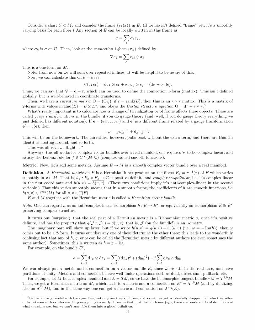
Consider a chart U ⊂M , and consider the frame ek(x) in E. (If we haven’t defined “frame” yet, it’s a smoothlyvarying basis for each fiber.) Any section of E can be locally written in this frame as

σ =∑k

σkek,

where σk is σ on U . Then, look at the connection 1-form (τij) defined by

∇ek =∑`

τk` ⊗ σ`.

This is a one-form on M .Note: from now on we will sum over repeated indices. It will be helpful to be aware of this.Now, we can calculate this on σ = σkek:

∇(σkek) = dσk ⊗ ek + σkτkj ⊗ ej = (dσ + στ)ej .

Thus, we can say that ∇ = d + τ , which can be used to define the connection 1-form (matrix). This isn’t definedglobally, but is well-behaved in coordinate transforms.

Then, we have a curvature matrix Θ = (Θij); if r = rank(E), then this is an r × r matrix. This is a matrix of2-forms with values in End(E) = E ⊗ E∗, and obeys the Cartan structure equation Θ = dτ − τ ∧ τ .8

What’s really important is to calculate how a change of trivialization or of frame affects these objects. These arecalled gauge transformations in the bundle, if you do gauge theory (and, well, if you do gauge theory everything wejust defined has different notation). If e = (e1, . . . , er) and e′ is a different frame related by a gauge transformatione′ = g(e), then

τe′ = gτeg−1 + dg · g−1.

This will be on the homework. The curvature, however, pulls back without the extra term, and there are Bianchiidentities floating around, and so forth.

This was all review. Right. . . ?Anyways, this all works for complex vector bundles over a real manifold; one requires ∇ to be complex linear, and

satisfy the Leibniz rule for f ∈ C∞(M ;C) (complex-valued smooth functions).

Metric. Now, let’s add some metrics. Assume E →M is a smooth complex vector bundle over a real manifold.

Definition. A Hermitian metric on E is a Hermitian inner product on the fibers Ex = π−1(x) of E which variessmoothly in x ∈M . That is, hx : Ex ×Ex → C is positive definite and complex sesquilinear, i.e. it’s complex linearin the first coordinate and h(u, v) = h(v, u). (These two conditions imply it’s anti-complex-linear in the secondvariable.) That this varies smoothly means that in a smooth frame, the coefficients of h are smooth functions, i.e.h(u, v) ∈ C∞(M) for all u, v ∈ Γ(E).E and M together with the Hermitian metric is called a Hermitian vector bundle.

Note. One can regard h as an anti-complex-linear isomorphism h : E → E∗, or equivalently an isomorphism E ∼= E∗

preserving complex structure.

It turns out (surprise!) that the real part of a Hermitian metric is a Riemannian metric g, since it’s positivedefinite, and has the property that g(J u,J v) = g(u, v); that is, J (on the bundle!) is an isometry.

The imaginary part will show up later, but if we write h(u, v) = g(u, v) − iω(u, v) (i.e. ω = − Im(h)), then ωcomes out to be a 2-form. It turns out that any one of these determine the other three; this leads to the wonderfullyconfusing fact that any of h, g, or ω can be called the Hermitian metric by different authors (or even sometimes thesame author). Sometimes, this is written as h = g − iω.

For example, on the bundle Cr,

h =

r∑k=1

dzk ⊗ dzk =

r∑k=1

((dxk)2 + (dyk)2

)− i

r∑k=1

dxk ∧ dyk.

We can always put a metric and a connection on a vector bundle E, since we’re still in the real case, and havepartitions of unity. Metrics and connection behave well under operations such as dual, direct sum, pullback, etc.

For example, let M be a complex manifold and E = TM , so we have the holomorphic tangent bundle τM = T 1,0M .Then, we get a Hermitian metric on M , which leads to a metric and a connection on E∗ = Λ1,0M (and by dualizing,also on Λ0,1M), and in the same way one can get a metric and connection on Λp,q(E).

8Be particularly careful with the signs here; not only are they confusing and sometimes get accidentally dropped, but also they oftendiffer between authors who are doing everything correctly! It seems that, just like our frame ek, there are consistent local definitions of

what the signs are, but we can’t assemble them into a global definition.

15

Adding Complex Structure. For now, let E →M be a complex vector bundle, where M is a real manifold (soonto be complex, but not yet), and let h be a Hermitian metric on this bundle.

Definition. A connection ∇ is called compatible with h if h is parallel (i.e. ∇h = 0) as a real tensor.

Equivalently, h is parallel iff it satisfies the Leibniz rule

dXh(u, v) = h(∇Xu, v) + h(u,∇Xv),

where X ∈ TM and u, v ∈ Γ(E).Now, suppose E →M is a complex vector bundle and M is a complex manifold; then, choose a complex linear ∇

in E. It can be decomposed along Λ1E = Λ1,0(E)⊕Λ0,1(E) (i.e. compose with projections): ∇ = ∇1,0 +∇0,1. Then,∇1,0 : Γ(E)→ Λ0,1(E) satisfies the following Leibniz rule:

∇0,1(f · σ) = ∂f ⊗ σ + f∇0,1σ.

There is a similar one for ∇1,0, but with ∂ instead of ∂.

Definition. If E is a holomorphic vector bundle, a connection ∇ is said to be compatible with the holomorphicstructure (sometimes compatible with the integrable structure) of E if ∇0,1 = ∂E .

Before we go on to the Chern connection, let’s look at this a little more. (∇0,1)2 = (R∇)0,2 (which can be computedby expanding (∇0,1 +∇1,0)2), i.e. just the (0, 2)-part of the curvature. In particular, this means that the (0, 2)-partof the curvature is 0 iff ∇ is compatible with the holomorphic structure. This should look like the proofs we did lasttime.

Proposition 6.1. Assume E →M is a holomorphic vector bundle and h is a Hermitian metric on E. Then, thereexists a unique connection ∇ on E, called the Chern connection, that is compatible with both the Hermitian structureof h and the holomorphic structure of E.

This plays a similar role to the Levi-Civita connection over real manifolds, but is compatible with more structure.

After we show this, the curvature of ∇ is of type (1, 1); we saw above that the (0, 2)-term is ∂2

E = 0, andunsurprisingly the (2, 0)-term comes from ∂2 = 0.

Proof of Proposition 6.1. The formula for the connection is

∇ = ∂E + h−1(∂E)∗ h.Here, we use h : E → E∗ (anti-complex-linear). Then, it suffices to check the compatibility conditions, e.g. incoordinates, though an intrinsic proof also works. This is the only possible one once the conditions are written down.

Since h : E → E∗ is anti-complex-linear, then h is ∇-parallel (because it’s compatible), i.e. ∇h = 0. Thus, if onetakes a section u of E, then by the Leibniz rule

∇(h(u)) = (∇h)(u) + h(∇u) = h(∇u),

and therefore h commutes with ∇; thus, by anti-complex-linearity, the (0, 1)-part has to be determined by ∂, and therest has to be determined by pulling back by h. Thus, this is unique.

If you don’t like this, we can do it in coordinates; we can choose either a holomorphic frame or a Hermitian frame.In a local frame, though, ∇ is determined by the connection 1-form τ , i.e. ∇ek = τkj ⊗ ej , so writing this as a columnmatrix, ∇e = τ ⊗ e.

If ek is a holomorphic frame, then let hij be the coefficients of h in this basis. Then, the compatibility condition

ensures that ∂h = τ · h and ∂h = hTτ , so τ = ∂h · h−1. Thus, in the unitary (Hermitian) frame, τ is skew-Hermitian.

7. Kahler Metrics: 1/27/15

Last time, we showed that if E →M is a holomorphic vector bundle and h is a Hermitian metric, then there existsa unique connection, called the Chern connection, that is compatible with the metric. We’ll use this next week inHodge theory, which is the theory of the Dolbeault cohomology H∗,∗(M,E), where M is a compact, complex manifold.This relates to an operator, known as the Hodge star, which provides a finite-dimensional version of Poincare duality(called Serre duality). We can also fix a metric h and consider the space of holomorphic structures given by vectorbundles E →M ; this is known as deformation theory.

But this is all later; this week we are going to talk about Kahler metrics. Today, we’ll take a special case of thediscussion last time, where M is a complex manifold and E = TM . Some Hermitian metrics on E will have a specialproperty and will be called Kahler metrics, though they don’t always exist. When they do, they have very specialproperties.

16

There are many equivalent definitions of Kahler metrics, and it will be helpful to pass between them. Just aswe showed the existence and uniqueness of the Chern connection last time, we’ll spend this lecture proving thesedefinitions are equivalent.

Definition. A Hermitian metric h = g − iω is called a Kahler metric if rhe Kahler form ω = − Imh is d-closed, i.e.dω = 0.

Theorem 7.1. The following are equivalent for a Hermitian metric h = g − iω.

(1) h is Kahler.(2) Locally, ω has a potential, i.e. ω = i∂∂u, called the Kahler potential.(3) h osculates to order 2 to the standard metric, i.e. at each z0 ∈M there exist holomorphic coordinates z on

M such that

hij(Z) = δij +O(|z|2).

(4) The Chern and Levi-Civita connections coincide.

For (3), recall that any Riemannian metric looks like a Euclidean metric in some coordinates (specifically, theRiemann normal coordinates) to first order, but here it’s possible to do better.

There are actually even more definitions and equivalences, but this seems like a reasonable place to start

Example 7.2.

• The flat connection or Euclidean connection on Cn is given by

h = i

n∑k=1

dzk ⊗ dzk =1

2i∂∂|z|2,

so it has a global potential, and is thus Kahler.• For an example with a local but not global potential, consider CPn with the standard Fubini-Study form

ωFS =i

2π∂∂ log(1 + |z|2), (3)

which is defined on Cn = CPn \H, where H is the hyperplane at infinity. This can be shown to extend toCPn, though this require some calculation. Nonetheless, thi illustrates that it has a local, but not global,potential.

There’s a better way to write it, though: we know about a projection π : Cn+1 \ 0→ CPn, quotienting byC∗, so we can describe the pullback

(π∗ωFS) =i

2π∂∂ log|z|2,

with z ∈ Cn+1 \ 0. Then, π sends (z0, . . . , zn) 7→ [z0, . . . , zn]. It’s a simple but useful exercise to show thatthese are the same notion, and that this one descends to the quotient.

Now, why is this Kahler? Clearly we have a local potential, but we need to check that we even have ametric. So, why is it positive definite? This comes after a calculation on (3):

2π

iωFS =

1

1 + |u|2∑k

duk ∧ duk +1

(1 + |u|2)2

(∑uk duk

)∧(∑

uk duk

).

This is a brute-force calculation, but one can see why it’s positive definite: when u = 0, lot of things cancel,and when u 6= 0, it’s possible to use a unitary transformation in U(n + 1) on C(n + 1) to rotate to thatparticular point: this form is homogeneous.9

Another nice thing about the Fubini-Study form is that if ` is a line, then∫`ωFS = 1. Thus, it has a

nonzero de Rham cohomology class [ω] ∈ H2(M ;Z), and is therefore Poincare dual to the line ` ∈ H2(M,Z).This can be generalized, but for CPn it’s particuarly nice.

Note. One can describe Aut(CPn), i.e. its biholomorphisms, as Aut(CPn) = PGL(n+1,C). In single-variable complexanalysis, this is just the description of Mobius transformations. Now, since the data of a Kahler form is the data of acertain Hermitian metric, then those biholomorphisms that fix ωFS are isometries, which come from U(n+ 1), andthese act transitively on CPn. Hence, CPn is homogeneous.

Corollary 7.3. If h is a Kahler form, then its restriction to a complex submanifold is still Kahler. In particular,every complex submanifold of CPn is Kahler.

9You can do the explicit calculation at a particular point, but do you really want to?

17

This follows directly from the definition: dω = 0, so dω|M = 0.For example, we mentioned earlier that complete intersections of hypersurfaces in CPn, i.e. transverse intersections

of zero loci of homogeneous polynpmials are complex submanifolds.10

Example 7.4. On the unit ball in Cn, there’s

ω =i

2π∂∂ log(1− |u|2).

After we discuss curvature, we’ll see that this metric has negative curvature.

Example 7.5. As a non-example, remember the Hopf manifold? When n ≥ 2, it ha no Kahler structure, which isbecause of a cohomology condition.

Fact. If M is a compact, Kahler manifold, then H2j(M,R) 6= 0 whenever j ≤ dimCM . This is because the Kahlermetric ω is d-closed, so [ω] ∈ H2(M) is nonzero, and it’s nondegenerate, so Λnω is a volume form on M , and so inthe top dimension, [ω]n 6= 0 in H2n(M).

Note. Kahler metrics also induce nonzero Dolbeault cohomology, which we will show later: Hj,j(M) 6= 0 if M isKahler. This follows for a very similar reason: ω is ∂-closed, so [ω] ∈ H1,1(M).

In Hodge theory, if ω is a Hermitian metric (not necessarily even Kahler), then ωn is still nondegenerate, and (thispart requires some argument) gives a nonzero class in Hn,n(M).

Note. A d-closed, nondegenerate 2-form on a real manifold is called symplectic; thus, all Kahler metrics are symplectics.In fact, symplectic is to Kahler as almost complex is to complex; both differ by an integrability condition, and anysymplectic manifold has an almost complex geometry.

Proof outline of Theorem 7.1. Let h be a Hermitian metric on a complex manifold (M,J ).That (1) is equivalent to (2) is the statement of the Poincare ∂∂ lemma, Lemma 4.3.That (1) follows from (3) is just a calculation. In the other direction, it’s a PDE: we want to find a holomorphic

change of coordinates ϕ to “kill” the 1-jet of h. It’ll end up being sufficient for ϕ to be holomorphic in z and z.First of all, there’s a linear cange of coordinates to make hij(0) = δij , i.e.

hij(z) = δij +∑

aijkzk + `(z) +O(|z|2),

where `(z) is some linear term that we don’t care about. Since h is Hermitian, it’s determined by the one in z, andis in fact its complex conjugate. But since dω = 0, then aijk = akji, which is an unpleasant, but not very difficult,calculation. Thus, just take

wj = zj +1

2

∑i,k

aijkzizk,

and just check it, though we won’t do this here. The idea is, since it’s merely quadratic, one can just make a solutionby hand.

Finally, that (4) ⇐⇒ (1) is a brute-force calculation, though it can be simplified somewhat; see Morianu’s book.Here are the main ideas:

• Both the Chern and Levi-Civita connections are compatible with the metric.• The Levi-Civita connection is torsion-free, though the Chern connection may not be. It turns out that the

torsion of the Chern connection is 0 iff dω = 0.• J is compatible with respect to Chern (which is sometimes taken as a definition of the Chern connection),

though the Levi-Civita connection may not be. It turns out that the Levi-Civita connection is parallel iffNJ = 0 and dω = 0.

We won’t provide all of the ingredients of this calculation, but the ingredients will all be provided, so that checkingthe rest is simpler. Recall that the torsion of a metric is T (X,Y ) = ∇XY − ∇YX − [X,Y ], and the Levi-Civitaconnection is the unique torsion-free connection compatible with a given Riemannian metric g (i.e. ∇g = 0); similarly,the Chern connection is the unique connection compatible with a Hermitian metric h = g − iω, i.e. ∇h = 0 andR0,2∇ = 0. Thus, ∇g = 0, ∇ω = 0, since ω = g(J ·, ·).Recall also that the curvature for a Riemannian manifold was RXY = ∇X∇Y − ∇Y∇X − ∇[X,Y ], and if ∇ is

torsion-free and ω is a k-form, then

dω(X0, . . . , Xk) =∑k

(−1)k∇Xk(ω)(X0, . . . , Xk, . . . , Xn).

10In differential geometry, the term “transverse intersections” is used, and in complex or algebraic geometry, one sees “completeintersections.” You also might want to intersect more general holomorphic functions in this definition, but these end up only being

polynomials, anyways!

18

(Here, Xk means the absence of index k.)Thus, since ∇g = 0 and ∇ω = 0 for the Chern connection, then ∇J = 0, so (as was on the homework), the (1, 1)

part of the torsion T vanishes. Since torsion basically measures the difference between dω and ∇ω, then the torsion isonly (0, 2).

Thus, one can prove two lemmas. Assume h is Hermitian on an almost complex manifold and ∇ is the Levi-Civitaconnection.

Lemma 7.6. There exists a connection ∇XY = ∇XY − (1/2)J (∇XJ )Y , which is a connection preserving g and J ,but has torsion T = −(1/4)NJ .

Lemma 7.7. ∇J = 0 iff NJ = 0 and dω = 0.

Proof sketch of Lemma 7.6. This is yet another calculation, using

• the Leibniz rule,• that g(J ·,J ·) = g(·, ·), and• J 2 = − id, so ∇J and J anticommute.

Once we address Lemma 7.7, then all of the required equivalences are proven.

8. Curvature on Kahler Manifolds: 1/29/15

“I’ve forgotten how to do logic.”

Recall that last time, we showed that the Levi-Civita connection is equal to the Chern connection iff M is Kahler.We provided much of the proof, but not all of it.

Lemma 8.1. Let M be a complex manifold, h a Hermitian metric, and ∇ the Levi-Civita connection. Then, ∂ for

∇, regarded as ∂∇

: Γ(TM )→ Λ0,1(TM ) is

∂∇VX =

1

2(∇VX + J∇JVX − J (∇V J )(X)). (4)

Corollary 8.2. In particular, if M is Kahler, then the Levi-Civita and Chern connection coincide.

This is because in this case, J is parallel to ∇, and therefore terms drop out and the same expression holds.

Proof of Lemma 8.1. Though one could calculate this by brute force, there’s a cleverer way to do this, involving thelinearization of the holomorphic map equation at the identity. This is defined in the following way: if ϕ : M →M isholomorphic, then

0 = ∂ϕ =1

2(dϕ+ J dϕ J ),

which is equivalent to ϕ∗J = J .Thus, the following one-parameter family of variations is a vector field:

X =d

dt

∣∣∣∣t=0

ϕt.

But be careful with this linearization: J may not be parallel, so we have to keep track of its variation. Thus, when

we linearize, it ends up being ∂∇X = 0, where ∂

∇is exactly a in (4).

If one linearizes the condition ϕ∗J = J instead, then it’s just the Lie derivative, by definition:

0 = LXJ =d

dt

∣∣∣∣t=0

(ϕ∗J ).

Thus, X is a holomorphic vector field, i.e. an infinitesimal automorphism.Recall that Aut(M) is a Lie group, though it may be infinite-dimensional. Certainly id ∈ Aut(M), and we can

consider its tangent space Tid Aut(M). Recall back in differential topology, one did something similar: using theflow equation, Tid Diff(M) = X (M) = Γ(TM ) (smooth vector fields). This is a little weird, because this Lie group isdefinitely infinite-dimensional (in our case, it’ll be finite-dimensional). In any case, this tangent space is a Lie algebra,which will be useful; it’ll be important to make sense of this precisely, but it is useful motivation.

Exercise 8.3. Calculate the infinitesimal automorphisms (i.e. the biholomorphic ones) of CPn.

Back in the world of complex geometry, if M is a complex manifold, Tid Aut(M) = Xholo(M) = H0(M ; TM ), i.e.holomorphic vector fields. (Here, as always, TM is the holomorphic bundle, the (1, 0)-part).

Note. X is a Killing vector field if it is an infinitesimal isometry, i.e. in Tid Isom(M); and isometries are defined asg(ϕ(·), ϕ(·)) = g(·, ·), or, equivalently, ϕ∗g = g.

19

Exercise 8.4. Calculate the linearizations of both limits; this should agree with the standard definition of a Killingvector field.

Now, back to the proof. Remember that the Levi-Civita connection is defined on the real tangent bundle, andthe Chern connection is defined on the holomorphic tangent bundle, so one must pull them back and identify themsomehow to identify them. That is, we need T 1,0M ' TM , as an isometry of complex vector bundles.

Consider ψ : TM → T 1,0M given by X 7→ (1/2)(X − iJX) = Z. Then, Z 7→ X is called taking the real part.

Then, one can pull back the Levi-Civita connection by ψ−1 to get ∇ on T 1,0M . Then, with ∂∇

as in (4), one justchecks that it satisfies the Leibniz rule for ∂. Some care should be taken with ∂ versus d, but in the end, one canshow that (∂f)(X) = dZf for all f : M → C.

Finally, we need to check that this is ∂. This is done by looking at the holomorphic tangent bundle, and showing

that ∂∇Z = 0 is the same as the real part of X satisfying LXJ = 0.

Curvature. Curvature is very special for Kahler manifolds. Recall that in the real case, where E = TM , there’s theRiemann curvature tensor R(X,Y, Z,W ) = g(R(X,Y )Z;W ), with coefficients Rijk` = giRijk. There’s also the Riccitensor

Ric(X,Y ) = Tr(v 7→ R(v,X)Y ) =∑k

R(ek, X, Y, ek).

In a frame, this has coefficients Rij = Rkikj . Finally, there’s the scalar curvature = Tr(Ric) = Rijgij . There are other

curvatures, but we won’t worry about this; similarly, one can define these on almost complex or complex manifolds,but we’ll go directly to the Kahler case.

Now, let M be a Kahler manifold, and ∇ denote the Levi-Civita (and therefore also Chern) connection.

Definition. The Ricci form is ρ(X,Y ) = Ric(JX,Y ).

Proposition 8.5. ρ is a closed 2-form, and agrees with i · TrC(R∇).

Therefore it has a geometric interpretation: in cohomology, [ρ] = 2πc1(M) (that is, it represents the first Chernclass), or equivalently,

c1(M) =i

2π[TrR∇] =

1

2π[ρ].

This follows from Chern-Weil theory, which we’ll discuss later on; one could also take it as a definition. That thisclass is independent of the choice of Kahler metric, which is a good exercise.

This is also related to U(n) holonomy and parallel transport, which we’ll expand on later.Another application of curvature is the notion of Kahler-Einstein metrics, which show up in physics. In the real

case, the Einstein equation is Ric = λg for a constant λ, and the analogous equation for Kahler manifolds is theKahler-Einstein equation ρ = λω (with the Ricci and Kahler forms). Since the right-hand side is positive definite,then the left-hand side is required to be as well. This relates to the special notion of a Ricci-flat metric, where ρ = 0everywhere, and the Calabi-Yau theorem.

Note. If E →M is a complex vector bundle and ∇ is a complex connection, then R∇ ∈ Λ2(M,EndC(E)) (that is, it’sa two-form), so one can take its complex trace TrC : EndC(E)→ C, yielding a two-form on M (with values in thetrivial bundle), TrR∇ ∈ Λ2(M).

Here are some useful properties, even if they may be a little simple.

Proposition 8.6. Let M be a Kahler manifold.

(1) Ric(JX,J Y ) = Ric(X,Y ).(2)

Ric(X,Y ) =1

2TrR(R(X,Y ) J ).

(3) ρ is real (1, 1) and closed; ω is also closed (1, 1).(4) ρ = iTrC(R∇) for the holomorphic vector bundle E = TM .11

(5) In holomorphic coordinates, if H is the matrix of h, then

ρ = −i∂∂ log det(H).

(6) Intrinsically, ρ represents c1(TM ) = −c1(KM ); specifically,

c1(TM ) = c1(detC

TM ) =i

2π[TrC(R∇)] =

1

2π[ρ].

11Here, R∇ ∈ Λ1,1(End(TM )), so taking the trace gives something in Λ1,1(M), as before.

20

Proof. (1) follows because J is parallel, and then follows from properties of R, so it can be calculated in an orthonormalbasis ek (or even better a unitary basis).

Specifically, since R∇ is complex linear, then

R(X,Y,JZ,JW ) = R(X,Y, Z,W ) = R(JX,J Y,Z,W ).

Then, substitute in a basis and take the trace.(2) requires more work. Use the first Bianchi identity,12 which says that cyclic permutations of the terms in

R(X,Y, Z, ·) don’t affect the result. Then,

Ric(X,Y ) =∑k

R(ek, X,J Y,J ek)

= mess−R(J Y, ek, X,J ek),

and when the mess of terms simplifies, it ends up being the formula we wanted.For (3), use (1), which implies that ρ is (1, 1); then, by the second Bianchi identity, ∇R∇ = 0, and dρ can be

written as a combination of terms in ∇ρ, so therefore dρ = 0.

(4) is (2) plus some linear algebra: for a skew-Hermitian matrix A, one can write A =

(0 −ARAR 0

); then, A = ARJ ,

so iTrC(A) = TrR(AR J ). Then, apply the spectral theorem. This follows because since A is skew-Hermitian, then

A = −AT, i.e. A ∈ u(n), which is equivalent to iA being Hermitian.

Another way to think of this is that Tr : u(n)→ iR. Recall that in a unitary frame, the matrix of one-forms τ andthe curvature matrix Θ are both skew-Hermitian, i.e. τ,Θ ∈ u(n). This has connections to representations of Liegroups! τ ∈ Λ1(Ad(E)), and Θ ∈ Λ2(Ad(E)).

There are sometimes sign errors or missing factors of i, relating to the fact that the natural Lie algebra of S1 is iR,but people often write it as R, so things can get muddled.

Anyways, we get exp : u(n) → U(n), and the associated log, and so log det(A) = Tr(logA). This is the insightbehind Chern-Weil theory, and in particular when one does a brute-force calculation in a basis, then (5) falls out.This involves pushing around Christoffel symbols.

Γiki =1

2gim

∂gim∂xk

=1

2g−1

∂g

∂xk= d log

√det g.

For the Kahler case, of course we’ll compute in a unitary frame, and let hij be the coefficient of dzi ⊗ dzj , so that

hij = hij . Then, because T 1,0M is ∇-parallel, all mixed Christoffel symbols are 0. There’s more calculation to be

done, e.g. R∇ is of type (2, 2), and so on, so a lot of terms drop out.

9. Hodge Theory: 2/3/15

This will seem like a considerable digression from Kahler metrics, but the two come together and interplay ininteresting ways. It would be nice to talk about them simultaneosly, but this is as close as one can get.

Hodge theory is a way of analyzing various cohomology theories on complex manifolds. We’ve already seen severaldifferent complexes in this context:

• When M is a real manifold, there’s the de Rham cohomology d : Ak(M)→ Ak+1(M).• When M is a complex manifold, there’s the Dolbeault cohomology ∂ : Ap,q(M)→ Ap,q+1(M).• The Dolbeault cohomology could also be contstructed as ∂ : Ap,q → Ap+1,q.• Finally, if E →M is a holomorphic vector bundle, then Dolbeault cohomology with coefficients in E i given

by maps ∂E : Ap,q(M ;E)→ Ap,q+1(M ;E).

The commomalities are an operator D (d or ∂ or ∂), which is a first-order linear differential operator, such thatD2 = 0. Thus, one can take the cohomology of this complex, which is D-closed forms modulo D-exact forms.

Then, for every α ∈ Ap,q (or more generally the objects in the complex), there’s an induced [α] ∈ Hp,q(M) (ormore generally, the homology group), given by [α] =

α+ ∂ϕ | ϕ ∈ Ap,q−1(M)

. Today’s question is: is there a best

representation for this cohomology class? In general, no, but with the choice of a metric there does end up being agood choice.

Our goal is to prove that if M is compact, dimHp,q(M) is finite, and there will be a version of Poincare duality,called Serre duality. This involves the pairing Ak ×An−k → C, given by

(α, β) 7−→∫M

α ∧ β.

12. . . which was discovered by Ricci, not Bianchi, but whatever.

21

In order for these integrals to make sense, we’ll assume M is compact (otherwise, one could take compactly supportedsections, I suppose).

This is completely intrinsic, and descends first of all to a pairing Ap,q ×An−p,n−q → C, with the same formula, andthen to cohomology, e.g. Hk

dR(M)×Hn−kdR (M)→ R for de Rham cohomology and Hp,q(M)×Hn−p,n−q(M)→ C for

Dolbeault cohomology. We will prove this is nondegenerate; then, the canonical representatives will (in the presenceof a metric) lead to a way of passing between the two cohomology classes.

Thus, fix a metric (Riemannian for de Rham; Hermitian for Dolbeault). Then, there’s another pairing

〈α, β〉 =

∫M

〈α(z), β(z)〉dV, (5)

where dV is a volume form. This just takes the pointwise inner product and integrates it, and is called the L2 innerproduct on Ak. This means there’s a norm ‖α‖ = 〈α, α〉; is there a representation of [α] that minimizes the norm (orequivalently, the norm squared)? The goal is to find

minϕ‖α+Dϕ‖2,

which is basically a variational problem. It’s basically an orthogonal projection of α onto the space of exact forms.

Lemma 9.1. Assume α minimizes the norm in [α]. Then, 〈α,Dψ〉 = 0 for all smooth ψ.

In some sense, these are the Euler-Lagrange equations for this problem.

Proof. If α is the minimum, then for t ∈ R,

d

dt

∣∣∣∣t=0

‖α+ tDψ‖2 = 〈α,Dψ〉+ 〈Dψ,α〉.

This is sufficient for a Riemannian inner product, but if 〈·, ·〉 is Hermitian, then all we know is that the real part is

zero. For the imaginary part, one should minimize over complex lines, i.e. t ∈ C (or just using ‖α+ itDϕ‖2), afterwhich the same calculation shows the imaginary part is zero.

Definition. Let E,F →M be vector bundles over a manifold M , and D : Γ(E)→ Γ(F ). Then, fix metrics on E,F , and M , which creates an L2 inner product on Γ(E) and Γ(F ), once again given by (5). Then, the (L2) formaladjoint of D is D∗ : Γ(F )→ Γ(E) defined as

〈Dα, β〉 = 〈α,D∗β〉,for all compactly supported smooth section α ∈ Γ(E) and β ∈ Γ(F ).

It will also be useful that the adjoint of D∗ is equal to D.

Note. It’s easy to show that if it exists, then it’s unique, by some formal nonsense, but in our case, it’s possible tocalculate D∗, using integration by parts, Stokes’ theorem, and the Hodge star operator.

It will also end up that D∗ is a first-order differential operator; D as an operator on L2 is unbounded, which meansfutzing around with Sobolev spaces, and so on.

In summary, here’s what we’ve bought so far.

• Finding the “best” representation for [α], when α is closed, boils down to solving D∗α = 0 and Dα = 0.• Thus, it boils down to solving ∆α = 0, where ∆ = DD∗ +D∗D is the Laplacian.

These are equivalent by some formal nonsense.

〈∆α, α〉 = 〈DD∗α, α〉+ 〈D∗Dα,α〉

= ‖D∗α‖2 + ‖Dα‖2.Thus, ∆α = 0 iff Dα = 0 and D∗α = 0.

Definition. A solution of ∆α = 0 is called a harmonic.

The space of harmonics depends on what cohomology theory we’re talking about: for Dolbeault cohomology, the(p, q)-harmonics are Hp,q =

x ∈ Ap,q | ∆∂α = 0

, i.e. solutions to ∂α = 0 and ∂α = 0.

This is a little messy, since there are multiple cohomology theories floating around, and in general they’re differet.But in the case of Kahler manifolds, the harmonics are all the same!

Proposition 9.2.

• The minimum norm of [α] is achieved for a harmonic α.• ∆ is formally self-adjoint, and semipositive definite.

22

This boils down to solving the equation ∆α = 0.

Note. If a minimal α exists, then it is unique: such an α satisfies

‖α+Dϕ‖2 = ‖α‖2 + ‖Dα‖2 + 〈α,Dϕ〉+ 〈Dϕ,α〉 ≥ ‖α2‖,

and they’re equal iff Dϕ = 0.

Thus, all of the work goes into showing the existence of a minimal element, i.e. solving ∆α = 0. Here’s an outline.

• First, one can show the existence of a weak solution.• Then, regularity implies that a weak solution is smooth and a strong solution. This crucially uses the fact

that ∆ is an elliptic operator (which has to be checked separately for each cohomology theory) is an ellipticoperator, and therefore one can use the spectral theorem for self-adjoint, elliptic operators.

The second step is less PDE theory and more linear algebra: given that ∆ is self-adjoint and elliptic, one can considerits eigenspaces, satisfying ∆α = λα. These are finite-dimensional eigenspace, and the eigenvectors are smooth; thus,the spectrum is discrete, and there’s an L2-orthogonal decomposition into eigenspaces, which helps greatly in findinga solution.

Here, we require M to be compact; otherwise, ∆ wouldn’t be elliptic.

Theorem 9.3 (Hodge). Assume M is a compact, complex manifold, and fix a Hermitian metric. Conisider theLaplacian ∆ : Ap,q(M)→ Ap,q(M) from the Dolbeault cohomology and the harmonics Hp,q = ker(∆). Then:

(1) Hp,q is finite-dimensional.(2) There is a well-defined orthogonal projection h : Ap,q → Hp,q, inducing an isomorphism Hp,q ∼= Hp,q.(3) There exists a unique operator G : Ap,q → Ap,q such that:

• G|Hp,q = 0,• G∂ = ∂G,

• G∂∗ = ∂∗G, and

• I = h+ ∆ G.The last condition gives a sort of orthogonal decomposition.

(4) There is an orthogonal decomposition

Ap,q = Hp,q ⊕ ∂Ap,q−1 ⊕ ∂∗Ap,q+1

α = h(α) + ∂(∂∗Gα) + ∂

∗(∂Gα).

The operator G in (3) is called Green’s operator.

Note. The same theorem works with minor, predictable modifications for de Rham theory and the other cohomologytheories listed at the beginning of the class.

In order to dig into the proof, it’s necessary to understand what D∗ (in this case, ∂∗) is doing. Here’s where the

Hodge star comes in; it’s some more linear algebra.Given a real manifold M , fix a metric, so that there’s the rescaled L2 inner product on Ak given by

〈α, β〉 =1

k!

∫M

〈α(x), β(x)〉dVol ,

where dVol =√

det gij dx1 . . . dxn is a volume form.

If ei is a basis of a vector space V , then eI = ei1 ∧ · · · ∧ eik is a basis of ΛkV .

Definition. The Hodge star operator ? : Ak → An−k is defined by 〈α, β〉 = (α, ?β), i.e.

1

k!

∫M

〈α, β〉dVol =

∫M

α ∧ (?β).

This comes out sending basis vectors to basis vectors: let eIc denote wedging together all of the ej that aren’tcontained in the multi-index eI . Then, ∗eI = ±eIc , where the sign is the sign of the permutation (I, Ic) (in Sn)).

The Hodge star has some nice properties.

• ?( dVol) = 1.• ? is an ieometry, i.e. 〈?α, ?β〉 = 〈α, β〉.• ?2 = (−1)k(n−k) on Ak, i.e. ? is self-adjoint up to sign.• If M is complex, ? : Ap,q → An−q,n−p.

23

This means the following diagram commutes.

AkOO

?

d //Ak+1

d∗oo OO

?

An−k An−k−1doo

Lemma 9.4. d∗ : Ak+1 → Ak is given by the formula d∗ = −(−1)nk ? d?. Similarly, ∂∗

= − ? ∂?.

Thus, there’s a similar commutative diagram for the complex case. Thee both follow from Stokes’ theorem.

10. The Hard Lefschetz Theorem: 2/5/15

11. Line Bundles and Chern Classes: 2/10/15

Today, we’ll finish the proof of the Hard Lefchetz theorem, and discuss line bundles and Chern classes.Recall that if M is a Kahler manifold and ω is a Kahler form, then the Lefschetz operator Λ· = ωΛ·, so

L : Ap,q → Ap+1,q+1. Then, adj Λ = L∗.Let H be the counting operator H(ω) = (K − n)η when η ∈ AK(M) and n = dimCM . This shifts the dimension

down.Recall that the Lie algebra sl2 consists of trace-free 2× 2 matrices, with a generating set

X =

(1 −10 0

), Y = X∗ =

(0 01 0

), h =

(1 00 −1

),

satisfying certain commutativity relations [X,h] = 2X, [Y, h] = −2Y , and [X,Y ] = h (which is easy to check).

Lemma 11.1. If M is a Kahler manifold, then:

(1) [L,H] = 2L, [Λ, H] = −2Λ, and [L,Λ] = H; thus, these form an sl2-representation.(2) This descends to cohomology: [L,∆] = [Λ,∆] = 0.

Both parts are fairly easy to directly check.

Theorem 11.2 (Hard Lefschetz theorem). If M is a compact Kahler manifold and n = dimCM , then Lk :Hn−k(M)→ Hn+k(M) is an isometry, and both the de Rham and Dolbeault cohomnologies are sl2(Z)-representations.

Example 11.3. For H∗(CP1) (which is on the homework. . . cough), both H0,0 and H1,1 are one-dimensional, andthe rest are zero. Something similar happens in H∗(CPn).

Corollary 11.4. If M is a complex submanifold of CPN and h ⊆ CPN are hyperplanes, then Λhk : Hn+k(M) →Hn−k(M) is an isometry (where hk is the intersection of the k planes in homology), and the Poincare dual to theFubini-Study form is PD(ωFS) = h.

This is a homological restriction on the existence of a Kahler structure of a manifold, and is useful for proving thatsome manifolds don’t have a Kahler structure. There are several other, similar Lefschetz theorems, which also involveintersection theory.

Note. The irreducible representations of sl2 are classified by dimension, with exactly one in each dimenion: the trivialone C, the fundamental representation V (1) = H∗(CP1), and more generally the nth one is n+ 1-dimensional andgiven by V (n) = H∗(CPn) = Symn(C2).

Since H is just a shifting operator, then these decompose into eigenspaces for H:

V (n) = V−n ⊕ V−n+2 ⊕ · · · ⊕ Vn−2 ⊕ Vn.These are the eigenspaces for H; each is a copy of C, so L and Λ commute with them, and shift from one to the next.Thus, at some point, it terminates with ker(Ln+1). Similarly, V−n is ker(Λ) intersected with the eigenspace of H.These subspaces are called primitive.

Definition. The primitive cohomology P ∗ ⊆ H∗ is P ∗ = ker(Λ) ∩H∗.Thus, there is a decomposition

Hk =⊕p

LpP k−2p.

One can also use this to realize the Riemann bilinear pairing (for a Kahler manifold): instead of a skew-symmetricbilinear form Q(α, β) =

∫Mα ∧ β, one can instead create one on Hk by

Q(α, β) =

∫M

α ∧ β ∧ ωn−k.

24

This is Hermitian; H(α, β) = ikQ(α, β). This is a very useful technique for studying Kahler manifolds further, thoughwe won’t use it any more.

Line Bundles. The goal for today is to understand complex or holomorphic line bundles up to isomorphism, includingwhen they’re isomorphisms or classifying them. Line bundles are easier to deal with than higher-dimensional cases,but it’s nice to have them too.

There are several approaches to line bundles; they’re all useful in different contexts.

• One way is via transition functions, which ends up in a 1-Cech cocycle.13

• Another way is as zeros of open sections, though in the holomorphic case it’ll be necessary to considermeromorphic functions, and tracking zeros and poles with multiplicity. This leads to a notion of divisors.

• One very good way is via the first Chern class, which is the Euler class, and relates to both of the previousapproaches, the first via an exponential function, and the second thanks to Poincare duality, By Chern-Weiltheory, it also relates to curvature.

We will spend the most time working on the third approach.One important question: is there a difference between isomorphism as complex line bundles and as holomorphic

line bundles? Relatedly, how many different holomorphic structures can one place on the same complex line bundle?Typically, they’ll come in families. This leads to deformation theory: deformations of holomorphic structures, moduliproblems, and Kodaira-Spencer theory. But this is just motivation.

Definition. Let M be a complex manifold. Then, the Picard group Pic(M) is the set of holomorphic line bundles,up to isomorphism; here, multiplication is given by L1, L2 7→ L1 ⊗ L2 and inversion by L1 7→ L∗1. Then, Pic0(M) orJac(M), called the Jacobian, is the subgroup of topologically trivial ones.

Before presenting some massive theory, it’s good to have some concrete examples in mind.

Example 11.5. We can show that Pic(CPn) = Z, generated by the tautological line bundle (from Dolbeaultcohomology), and therefore Pic0(CPn) = 0. Thus, isomorphism as holomorphic line bundles over CPn is the same asisomorphism of smooth, complex line bundles over CPn.

However, on an elliptic curve E, that’s no longer the case; there exists a one-parameter family of holomorphic linebundles which are all topologically trivial (and therefore isomorphic as complex line bundles). Another way to saythat is that the moduli space is one-dimensional. In particular, Pic0(E) ∼= E, with the isomorphism canonical as soonas the origin is chosen. This will be as topological spaces (where Pic0(E) happens to have a natural topology andbecomes a one-dimensional complex manifold), but we don’t know that yet.

Topologically, think of an elliptic curve as a torus; then, given a point p ∈ E, one can product a holomorphicline bundle O(p) which has a holomorphic section that has a simple zero at p and nowhere else. Then, O(p− q) =O(p)⊗O(q)∗ (because of where the simple zeroes are, and such); this is topologically trivial, but not holomorphicallyso when p 6= q; if it were, then there would exist a meromorphic f on E with a simple zero and a simple pole, whichisn’t possible, since it gives a degree-1 map f : E → CP1.

This is just like in complex analysis: on the sphere there is one unique complex structure, and on the torus there’sa one-parameter family of them. The reasoning is basically the same (Dolbeault cohomology).

Recall that for a line bundle the transition functions take the form gαβ : Uα ∩ Uβ → C∗ = GL(1,C).14 Thesemaps can be required to be smooth or holomorphic, depending on the kind of bundle. Note that we want this to becovariant, so gαβ is a transition from β to α.

On the intersection of Uα, Uβ , and Uγ , they satisfy a 1-Cech cocycle condition, that gαγ = gαβ gβγ .

In particular, gαα is the identity and gβα = g−1αβ . Thus, the above cocycle condition can be rewritten in the equivalent

form gαβ gβγ gγα = 1. Thus, the transition functions give a class in the one-dimensional Cech cohomology of (the

cover of) the manifold, with values in O∗, the nowhere vanishing holomorphic functions. That is, (gαβ) ∈ H1(M,O∗).

Theorem 11.6. There is a natural group isomorphism Pic(M) ∼= H1(M,O∗).O∗ is a sheaf, a generalization of a bundle, and whenever there’s a sheaf, there’s the exponential sequence

1 // Z // O

exp // O∗ // 1

where exp : f 7→ exp(2πif). This is a short exact sequence, and therefore there’s a long exact sequence in cohomology:

H1(M,O) // H1(M,O∗) δ∗ // H2(M,Z) // · · ·

13If you haven’t seen Cech cohomology before, it’s worth reading up on sheaves and cohomology in Griffith and Harris, §3, or in

Huybrechts.14“Linear algebra is just the representation theory of GL(n,C); we’ll do the representation theory of GL(1,C).”

25

Then, (gαβ) ∈ H1(M,O∗), and, as we’ll see, the first Chern class is in H2(M,Z). This sequence, and the relatedtechnique of Chern cohomology, can be used to more efficiently prove things such as the results in Example 11.5.

A section s in a line bundle is a collection of sα : Uα → C, required to be smooth or holomorphic dependingon context, so that sα = gαβsβ (which is where it’s nice to have the signs right!). A nowhere vanishing section

corresponds to a global trivialization of the bundle, and also corresponds to Cech-exact functions sα : Uα → C∗. Inparticular, the space of trivializations corresponds to H0(M,O∗) (which we’ll say more explicitly next time).

A good way to think of H0 is as holomorphic automorphisms of the line bundle; in particular, H0(M,O∗)corresponds to holomorphic, nowhere vanishing global function on M ; if M is compact, all such functions are constant,and in this case H0(M,O∗) = C∗.

Chern classes. There are many different definitions of Chern classes; they satisfy a universal property, so they canbe axiomatized; there’s also a definition in terms of classifying spaces, which is possibly the best, but definitely thescariest; and in this class, we’ll use Chern-Weil theory, which involves curvature.

In any case, they have universal properties, are topologically invariant under (continuous, but we only careabout) smooth isomorphism of complex vector bundles, and come from obstruction theory. Thus, they’re usefulfor understanding things such as whether two bundles are isomorphic, or whether one is trivial, and so on. Mostinterestingly, though, is whether a bundle has a nowhere vanishing section (given by the top Chern class), or k such(globally) linearly independent sections?

Chern classes are defined for any continuous complex vector bundle over a topological space, though we’ll usesmooth bundles over complex manifolds.

Definition. Let E →M be a smooth bundle over a complex manifold M ; then, the first Chern class c1(E) ∈ H2(M,Z)is the unique element that satisfies the following axioms.

(1) Naturality: c1(f∗E) = f∗(c1(E)).(2) Sums: c1(E ⊕ F ) = c(E)⊕ c1(F ).

(3) Normalization: c1(τ) = −h, where τ → CP1 is a tautological line bundle, and h ∈ H2(CP1,Z) is the generator,Poincare-dual to the point, i.e. ∫

CP1

c1(τ) = −1.

These will also imply how c1 behaves with products, which isn’t an axiom: c1(L1 ⊗ L2) = c1(L1) + c1(L2).Surprisingly, it’s also additive.

We don’t want to think too much about category theory, but the assignment c1(E) from a complex vector bundleE is functorial. Here are some more properties:

• Normalization also implies that c1(τ) = −h for τ → CPn the tautological line bundle, which is somewhatimmediate from restriction to CP1.

• But more interestingly, recall that det(E) = Λtop(E); then, c1(detE) = c1(E), which is a property we willend up using.

All of these properties follow from something called the splitting principle and the other axioms. This has nothingto do with complex analysis, but is good to know; a good reference is Bott and Tu. While it’s not true that everycomplex vector bundle splits as a direct sum of line bundles, but after a pullback to something called a splittingmanifold M(E), it does so, and this splitting manifold is a canonical construction (that does depend on the bundle),and then one can pushforward.

The basic idea of the splitting manifold is that if one pulls E back to itself, it has a canonical section σ(x, e; e) = (x, e)(this is a map E → π∗E), and this descends to the projectivization P(E) of E, and thus splits off a line bundle; then,repeat this process.

There are two more useful properties worth mentioning; we might actually prove them later.

• c1 is a complete topological invariant for smooth line bundles, i.e. E ∼= F iff c1(E) = c1(F ).• c1(L) = χ(L) is the Euler class, which is the Poincare dual of the generating section.

Next time, we’ll construct all of the Chern classes using curvature.

12. 2/12/15

13. Sheaves and Cech Cohomology: 2/17/15

“Algebra. . . whatever.”

Next time, we will discuss divisors and line bundles, albeit not in a whole lot of detail, since it relies on commplexanalysis we haven’t talked about. To read more about this, read the appendix to Moroianu and §2.3 of Huybrechts.

26

But today, we’ll talk about sheaves, sheaf cohomology, and applications. Sheaves should be thought of asgeneralizations of bundles, especially the notion of things patched together like sections. We’ll define Cech cohomologyon sheaves, and show Dolbeault’s theorem, that H(M ; Ωp) ' Hp,q(M). It will also be helpful that a short exactsequence of these leads to a long exact sequence on cohomology.

These will be applied to classify holomorphic or complex line bundles, which relates to the 1-Check cocycle and the1st Chern class. This relates to obstructions and determining whether a given complex line bundle has a holomorphicstructure. This relates to somehow yet two more Lefschetz theorems.

Sheaves. Let M be a complex manifold. Recall that locally there are lots of holomorphic functions, but globallymaybe there are fewer. For example, if M is compact, they must be constant.

This motivates the sheaf of holomorphic functions on M . On each open U ⊆ M , let OM (U) be the space ofholomorphic functions on U . The usual example is that U = Uα is a chart, so that OM (Uα) ∼= OCn(ϕα(Uα)).

In many arguments, it was helpful to shrink the charts, which leads to the notion of germs of holomorphic functions.This is the stalk of the sheaf at any point x ∈M , i.e. the germ at x is OM,x = lim−→U :x∈U OM (U); that is, one considers

the holomorphic functions in any neighborhood of x, with two functions considered the same if they agree on anyopen neighborhood of U .

Note that this is an extremely informal argument; it would take perhaps six lectures to do everything properly andrigorously!

In the same way, one can consider O∗M , the sheaf of nowhere vanishing holomorphic functions on M ; Γ(E) = A(E),the sheaf of smooth sections on a smooth vector bundle E; and Ω(E) = O(E), the sheaf of holomorphic sections ofa holomorphic vector bundle E. There are more examples of sheaves, e.g. skyscraper sheaves, but we won’t worryabout them right now.

We’ve seen this before in Dolbeault cohomology; for example, Ap,q(M ;E) consists of smooth section of Λp,qM ⊗ E.

Definition. A sheaf F on a second-countable, Hausdorff topological space M is an association:

• To each open U ⊆M , associate a group (or vector space, or some algebraic gadget) F(U) = Γ(U,F), calledthe section of F over U .

• To each inclusion U ⊆ V of open sets, associate the restriction map rU,V : F(V )→ F(U), which is requiredto be a homomorphism.

These are required to satisfy the following compatibility conditions.

(1) rU,V rV,W = rU,W for all U ⊆ V ⊆W open, and rU,U = id.(2) The gluing axiom: if σi ∈ F(Ui) for i = 1, 2 agree on an overlap U1 ∩U2, then there is a σ ∈ F(U1 ∪U2) such

that σ|Ui = σi for each i.(3) The uniqueness axiom: if σ ∈ F(U1 ∪ U2) and σ|Ui = 0 for each i, then σ = 0.

Even though the geometric intuition is reasonably clear, the algebra takes some time to write down.The topological condition is satisfied by all smooth manifolds, which will be enough for this class.

Note. In the definition of a sheaf, if only axiom (1) is satisfied, the resulting structure is called a presheaf. This isequivalent to a contravariant functor from the open sets of M (with inclusions a morphisms) to the category of groups(or whichever algebraic structure we’re looking at).

Definition. The stalk or fiber at x is the generalization of germs: Fx = lim−→U :x∈U F(U).

One can define morphisms of sheaves and presheaves, and with a little care, exact sequences. For example, considerthe exponential sequence below:

0 // Z i // O

exp // O∗ // 0.

Here, exp : f 7→ exp(2πif). i is injective for all U , but is surjective only if U is “small enough,” e.g. if U = C∗, thenit’s not possible to take the logarithm for all z ∈ O∗(U). Thus, the naıve definition of an image of cokernel of a sheafis only a presheaf; be careful! However, the naıve notion of a kernel is fine.

Note. To each presheaf F , one can associate a sheaf F+, called the sheafification (the process is called sheafifying,which is fun to say), which is a completely algebraic procedure; if F is a sheaf, then F+ = F , and this manages to fixthe exactness problem raised just above.

Sheaf Cohomology. Technically, sheaf cohomology and Cech cohomology are two different things, but they will bepresented as one thing; specifically, we’ll be talking about the latter. These record the failure of local sections to glueglobally.

Fix a (pre)sheaf F over a smooth manifold M , and choose a locally finite cover U = Uα of M . For each finiteindex set I, let UI =

⋂α∈I Uα.

27

Then, define the Cech (co)chain complex

C0(U ,F)δ // C1(U ,F)

δ // C2(U ,F) // · · ·

in the following way: Ck is the set of sections on (k + 1)-overlaps: C0 =∏α F(Uα), and in general,

Ck =∏

|I|=k+1

F(UI).

Then, the (co)boundary operator is

(δσ)I =

k+1∑j=0

(−1)j(σI\j

)∣∣Ui.

It’s the alternating sum of looking at one less overlap. Of course, there are two different sign conventions, e.g.Huybrechts uses the opposite one.

So, you can check (or Cech) that δ2 = 0, and when one takes the (co)homology, one obtains the Cech cohomologyHq(U ,F) of the cover U with coefficients in F . Then, one can refine the cover U , which induces a chain homotopy, soone can take the direct limit to obtain the Cech cohomology of M .

Hq(M,F) = lim−→UHp(U ;F).

This is really exactly the same idea as constructing refinements of partitions to obtain the Riemann integral!Don’t Google Cech cohomology, because the first result is a bunch of really confusing category-theoretic words.

Unless you’re all about category theory, I guess.For example, H0(M,O) is the group of globally holomorphic functions, and H0(M,Z) is the set of locally constant

integer-valued functions.Short exact sequences (which one has to be careful with) induce long exact sequences as before. And the inclusion

from holomorphic sections to smooth ones induces the following commutative diagram.Short exact sequences (which one has to be careful with) induce long exact sequences as before. And the inclusion

from holomorphic sections to smooth ones induces the following commutative diagram.

H1(M,Z) // H1(M,O) //

H1(M,O∗) δ∗ //

H2(M,Z) // H2(M,O)

H1(M,Z) // H1(M,A) // H1(M,A∗) δ∗ // H2(M,Z) // H2(M,A)

(6)

Here are some results we’ll use, but not prove.

Proposition 13.1. If F is the sheaf of smooth sections in some bundle, then one can patch local sections, so if q > 0,then Hq(M ;F) = 0.

Thus, in particular, Hq(M ;A∗,∗) = 0.

Theorem 13.2 (Leray). If the cover is acyclic, then H∗(U ;F) = H∗(M ;F), i.e. Hq(UI ,F) = 0 for all q > 0 and Ifinite.

Proposition 13.3. The Cech and “usual” (e.g. singular) cohomologies on a manifold coincide: H∗(M ;Z) =H∗(M ;Z).

If one takes an acyclic resolution

0 // R // A0 d // A1 d // A2 // · · ·

it’s possible to use the Poincare lemma to prove the following.

Theorem 13.4 (de Rham). Hq(M ;R) = HqdR(M) (that is, the de Rham cohomology).

Theorem 13.5 (Dolbeault). Using the ∂-Poincare lemma, one can use the resolution

0 // Ωp // Ap,0

∂ // Ap,1∂ // Ap,2

∂ // · · ·

to show that Hq(M,Ω) = Hp,q(M).

Basically, on a manifold, all cohomology theories are very similar.Now, we can actually use this to do some complex geometry. If this was bewildering, keep in mind that one cares

about the Cech cohomology to keep track of how local sections do or don’t patch into global ones.28

Theorem 13.6 (Kodaira-Spencer). Complex line bundles on a smooth manifold M are classified up to isomorphismby [gαβ ] ∈ H1(M ;A∗) ' H2(M ;Z), with the isomorphism given by δ∗(L) = [c1(L;∇)] = c1(L), the first Chern class.

Holomorphic line bundles on a complex manifold M are classified by [gαβ ] ∈ H1(M ;O∗). Thus, there is a naturalisomorphism Pic(M) ' H1(M ;O∗).

Proof. First, look back at (6), using the exponential sequence for smooth or holomorphic functions. Since A has apartition of unity, so Hq(M,A) = 0 when q > 0. Thus, δ∗ is an isomorphism.

It’s important to check that a holomorphic (or smooth) line bundle and a choice of trivialization gives a 1-Cechcocycle, and its class is independent of trivialization; then, that any cocycle in H1(U) represent a line bundle trivializedover U ; and if a cocycle [g] is exact, then the bundle is trivial, i.e. if g = δ(ϕ), then gαβ = ϕβ/ϕα.

Last lecture, we showed this is equivalent to showing that ϕ is a nowhere zero section of L, and therefore isequivalent to a trivialization.

These can all be walked through, but it’s still unclear why δ∗(L) = [c1(L;∇)]. These follow from formulas weproved last time! This is a big diagram chase, with an appropriately big diagram I wasn’t able to write down in time.We have that c1(L,∇)− (i/2π)Θ and Θα = dτα, and also that τβ − τα = −d log(gαβ); see the last lecture for moredetails. It will also be helpful to have the calculation

δ∗g =1

2πi(log gαβ + log gβγ + log gγα).

But gαβgβγgγα = 1.

One ends up taking the double Cech-de Rham complex Cq(U , Ap) with values in Ap.

Corollary 13.7. If H0,2(M) = 0, then any complex line bundle has a holomorphic structure; if H0,1(M) = 0, thenthis structure is unique.

Proof. From the exponential sequence and Dolbeault’s theorem, Hq(M,O) = H0,q(M) for all q, so plug theassumptions into the sequence

H1(M,O) // H1(M,O∗) // H2(M,Z) // H2(M,O).

Theorem 13.8 (Lefschetz theorem on (1, 1)-classes). Assume M is a compact, Kahler manifold. Then, Pic(M)→H1,1(M) ∩H2(M,Z) surjects, i.e. for all γ ∈ H1,1(M,Z), there exists a holomorphic line bundle structure such thatc1(L) = γ; and moreover, for any real, closed (1, 1)-form ω such that [ω] = c1(L) there exists a Hermitian metricsuch that the Chern connection has c1(L,∇) = 0.

The proof is once again a big diagram chase, using the de Rham and Dolbeault cohomologies, as well as the∂∂-Poincare lemma.

14. 2/19/15

15. Special Holonomy and Kahler-Einstein Metrics: 2/24/15

Today, we’ll return to the differential-geometric world, rather than the algebraic geometry from the last fewlectures. The goal is to provide a holonomy condition for Kahler metrics and the Kahler-Ricci flat condition, whichrelates to the notion of a Calabi-Yau manifold. More generally, there are bundle versions of these, known as theHermitian-Einstein or Hermitian-Yang-Mills condition.

There will be a trichotomy of 0, positive definite, and negative definite made in the curvature; there will be a clearrelation between this and other properties, though we don’t have time to cover the relationship between the curvatureand stability.

Holonomy. If E →M is a bundle over a (real or complex) manifold M and ∇ is a connection on it, then there’s aparallel transport Pγ : Ex → Ey, where γ : [0, 1] → M is a path from x to y. Pγ is a linear isomorphism, and anyσ0 ∈ Ex can be uniquely extended to a parallel section σ(t) along γ, i.e. a solution to the ODE ∇γ(t) = 0 and initialcondition σ(0) = σ0.

That’s holonomy in complete generality; if γ is a loop (x = y), then Pγ is an automorphism, and it might notbe the identity; that is, Pγ ∈ GL(Ex). If one takes all possible loops γ based at x, the result is the holonomy groupHolx(E,∇) = Pγ (for loops γ based on x). Holx(E,∇) ⊆ GL(Ex). One can also define the restricted holonomysubgroup, which is generated only by contractible loops, in case it’s useful to have something with vanishing π1.

Holonomy is conjugate along paths; that is, if γ is a path from x to y, then Holy(E,∇) = Pγ Holx(E,∇) P−1γ .In particular, if M is connected, there is a well-defined (up to conjugacy) holonomy subgroup, called Hol(E,∇).

29

Flat Bundles. Like everything else in this class, we’ll barely cover this, and it would be nice to spend more time onthem.

A bundle is flat if its curvature is, which strictly speaking depends on the connection. In differential geometry, thecurvature is called R∇, but sometimes, this is called F , and flatness just means that R∇ = 0.

By Stokes’ theorem, on a flat bundle, holonomy is invariant under homotopy of paths relative to endpoints, whichis to say that it descends to the fundamental group π1(M); that is, this gives the holonomy representation (sometimescalled monodromy, though technically that’s a different word) π1(M,x)→ GL(Ex).

Note. As a corollary, the bundle is flat iff the restricted holonomy is trivial (which is why assuming a manifold issimply connected is nice). On a complex manifold, this also implies that all Chern classes are torsion, i.e. identicallyzero in H∗dR(M).

Note. If M is simply connected, so that holonomy and restricted holonomy are identical, then any flat (principal)G-bundle is trivial, i.e. it has a nonzero, parallel section. This is proven by existence and uniqueness of a solution toan ODE.

In general, if M isn’t simply connected, local parallel sections always exist, though they may not patch globally.Equivalently, a nice solution will exist on the universal cover, but it might not be well-defined on M itself.

Note. Holonomy identifies the moduli space of flat, principal G-bundles (up to isomorphism) with representationsπ1(M)→ G up to conjugacy; there is a one-to-one correspondence. In other words, given a representation, there issome sort of line bundle. The best reference for this is the paper by Atiyah and Bott.

For example, if G is a finite group, then a principal G-bundle (i.e. with a free G-action) is a regular cover, and thisis just a restatement of deck transformations and their relations to the fundamental group.

As another example, the moduli space of flat, holomorphic line bundles on a compact Riemann surface Σ isJacobian Pic0(Σ) = Hom(π1(Σ), S1) (where S1 is interpreted as an abelian group), since in this case, G = U(1) = S1,so it’s abelian, and there is no conjugacy. And since this descends to H1 as the abelianization, this is also H1(Σ, S1).

All of these facts are nice and important and pretty, though strictly speaking we won’t depend on them in thisclass.

Holonomy and Kahler Manifolds. Let M be a 2n-dimensional Riemannian manifold, E = TM , and ∇ be theLevi-Civita connection. Now, this means parallel transport is an isometry, because ∇ is metric-compatible, soHolx(M, g) is conjugate to a subgroup of O(2n).

Berger’s theorem is hopefully review from differential geometry; it classifies all possible holonomies on a simplyconnected, irreducible, Riemannian manifold.

Definition. A Riemannian manifold is irreducible if it isn’t a product of lower-dimensional Riemannian manifolds;equivalently, it gives an irreducible representation.

It’s possible to do the same thing for an n-dimensional complex manifold M with a Hermitian metric. Out ofBerger’s list, here are a couple possible holonomies.

• If the holonomy is U(n), the result is a Kahler manifold.• If the holonomy is SU(n), the result is a Ricci-flat Kahler manifold, i.e. a Calabi-Yau manifold.• If n is even, Sp(n/2) gives rise to a hyper-Kahler manifold (also known as a holomorphic symplectic manifold).

There are a few more, but these three are the most interesting to us, and we’ll focus in particular on the first two.The third case, though, is very special and very rare; it has rich properties, since it has so much symmetry, and infact it can be regarded as the quaternionic analogue of the Kahler condition! This theory is much more rigid, andit’s a special case of the second one, since Sp(n/2) ⊆ SU(n) ⊆ U(n), and indeed Sp(n/2) = U(n/2,H), which is asubgroup of U(n,C). For example, if n = 2 (since 1 isn’t divisible by 2), then Sp(1) = SU(2), so K3 surfaces and toriare hyper-Kahler.

For the rest of the class, we’ll focus on the first two.

Proposition 15.1 (Holonomy principle). Any holonomy-invariant (pointwise) tensor at TxM extends uniquely to aparallel tensor field on TM .

This follows, like so many before it, from the existence and uniqueness of a solution to a certain ODE.

Lemma 15.2. Let (M, g) be a 2n-dimensional real, connected manifold; then, it is Kahler iff Hol(M, g) ⊆ U(n).Moreover, if the holonomy is precisely U(n), this structure is unique: there exists a unique integrable almost complexstructure J such that (M,J , g) is Kahler.

30

Proof. Suppose M is Kahler. Then, ∇J = 0 (where ∇ is the Levi-Civita connection), and holonomy is complexlinear, which implies that Hol(M,x) ⊆ O(2n) and Hol(M,x) ⊆ GL(n,C), but the intersection of these two is U(n)(i.e. transformations which preserve the metric and are complex linear must be unitary). This was used implicitlyearlier in the class, during Chern-Weil theory.

The other direction is harder; suppose Hol(M) ⊆ U(n). Fix Jx, a complex structure on the fiber TxM . Then, sincethe holonomy is unitary, then Jx is holonomy invariant, so by the holonomy principle, there’s a unique extension to aparallel tensor J ∈ End(TM ). By the chain rule, this means J 2 is parallel, but at x, J 2 = − id, and − id is alsoparallel. But by existence and uniqueness, this means J 2 = − id everywhere, so J is an almost complex structureparallel with respect to the Levi-Civita connection; that is, ∇J = 0.

Now, g is parallel, so ω(·, ·) = g(J ·, ·) is parallel, too (the composition of parallel tensors is parallel), and thereforeit is also closed, and therefore M is Kahler.

Uniqueness is left as an exercise.

Note that this uses that the Levi-Civita connection is torsion-free, which is embedded within the implication∇ω = 0 =⇒ dω = 0.

Before talking about the Ricci-flat condition, there will be a brief intermission, to discuss Kahler-Einstein metrics.

Assume M is a Kahler manifold; then, there is the Ricci form ρ(X,Y )(1)= Ric(JX,Y )

(2)= iTrC(R∇). In local,

holomorphic coordinates, let H = Hi; then, ρ = −i∂∂ log det(H), where ∇ is the Chern connection on TM , not theLevi-Civita connection.

(2) implies that iρ is the curvature of the Chern connection on the canonical line bundle KM = Λn,0, and isthe determinant bundle of the holomorphic cotangent bundle. Using this, one can prove that the Chern formc1(KM ,∇) = (1/2π)ρ = −c1(TM ,∇), ultimately following from Chern-Weil theory; we stated it a month ago, butnow there is a proof (along with a proof for the expression for ρ in coordinates).

When (M, g) is Kahler, then (1) implies that g is Einstein (i.e. Ric(g) = λg) iff g is Kahler-Einstein (i.e. ρ = λω;in both cases, λ ∈ R, and it’s called the Einstein constant). Up to a factor of 2πi, ρ represents the first Chern class,so if g is Kahler-Einstein, then c1(M) = (λ/2π)[ω].

The Kahler-Ricci-flat condition, i.e. λ = 0, implies that c1(M) = 0 in H2dR(M). The Calabi-Yau theorem will

imply that the converse is true.This gives a restriction on c1(M) if M admits a Kahler-Einstein metric: it has to be 0, positive, or negative, in the

following sense.

Note. A real, (1, 1)-form α is positive (written, of course α > 0), if α(·.J ·) is positive definite; negative definiteness isdefined similarly.

For example, α = − Imh, if h is a Hermitian metric, is positive. Note that if α is closed, then it’s a Kahler form.

Note. Much of this discussion extends to special metrics on holomorphic vector bundles over Kahler manifolds. Thereare connections (no pun intended) to a variational problem and to applications within physics.

If E is a holomorphic vector bundle, h a Hermitian metric on E, and ∇ the Chern connection, then R∇ ∈Λ2(M ; End(E)), so, tracing R∇ in the M -direction using the Kahler metric, Trg(R

∇) ∈ End(E), so if σα is a basis of

E, then (Trg R∇)βα = Rβαig

i.

A Hermitian-Einstein or Hermitian-Yang-Mills metric on E is a solution to Trg(R∇) = λ id, for a constant λ ∈ R.

This is a nonlinear analogue to the Laplacian equation from Hodge theory.

Next time, we’ll talk about the Calabi-Yau theorem and its extensions, and talk about SU(n) holonomy.

31