MATH 145 NOTES

ARUN DEBRAYAUGUST 21, 2015

These notes were taken in Stanford’s Math 145 class in Winter 2015, taught by Ravi Vakil. I TEXed these notes up using vim, and assuch there may be typos; please send questions, comments, complaints, and corrections to a.debray@math.utexas.edu.

CONTENTS

1. Meta Stuff and an Overview of Algebraic Geometry: 1/5/15 12. Projective Space and Fractional Linear Transformations: 1/7/15 33. Diophantine Equations and Classifying Conics: 1/9/15 54. Quadratics and Cubics: 1/12/15 65. Cubics: 1/14/15 86. The Elliptic Curve Group and the Zariski Topology: 1/16/15 97. Affine Varieties and Noetherian Rings: 1/21/15 118. Localization and Varieties: 1/23/15 139. Hilbert’s Nullstellensatz: 1/26/15 1410. Affine Varieties: 1/28/15 1511. Affine Schemes: 1/30/15 1712. Regular Functions and Regular Maps: 2/2/15 1813. Rational Functions: 2/4/15 2014. Rational Maps: 2/6/15 2115. Varieties and Sheaves: 2/9/15 2316. From Rational Functions to Rational Maps: 2/11/15 2417. Varieties and Pre-Varieties: 2/13/15 2518. Presheaves, Sheaves, and Affine Schemes: 2/18/15 2619. Morphisms of Varieties and Projective Varieties: 2/20/15 2820. Products and Projective Varieties: 2/23/15 2921. Varieties in Action: 2/25/15 3122. Dimension: 2/27/15 3223. Smoothness and Dimension: 3/2/15 3324. The Tangent and Cotangent Spaces: 3/6/15 3525. Images of Regular Maps: 3/9/15 3626. The Fundamental Theorem of Elimination Theory: 3/11/15 3727. Chevalley’s Theorem: 3/13/15 38

1. META STUFF AND AN OVERVIEW OF ALGEBRAIC GEOMETRY: 1/5/15

“Well, sadly, we live in the real world, but if you put on your complex glasses. . . ”The thing about undergraduate algebraic geometry is that very few schools offer it, and perhaps strictly fewer should.The class has a potential to end in tears, so we’ll speak carefully about where these things can go wrong.

Algebraic geometry is a grand unified theory of mathematics; well, maybe not so unified. It’s very broad, and youhave to know a lot to understand it very well. We’ll try to make the only prerequisite Math 120, though it will alsorequire a lot of intestinal fortitude if that’s your only experience. Similarly, we’ll try to actually do interesting thingsand motivate them, so that it’s not too hand-wavy or without motivation.

Algebraic geometry, the language of varieties, still also applies to number theory and complex geometry in other ways.This deals with something called a scheme, which we’ll define and discuss, but most of the cases will be for varieties.

Given that the people in the classes have vastly different backgrounds, difficult problem sets for one person will bemore straightforward for others, so we’ll have traditional problem sets along with maybe some other things. Perhaps wecan have a source of course documents or information in which people can edit other people’s documents, and people can

1

take (or even live-TEX!) notes for the class. This, along with problem sets and learning about some enrichment beyondthe lectures, will play into the course grade.

While we’re not going to follow a single book, there is a sort of canonical set of things to do, and here are some usefulreferences to have; all of them are freely and legally available online to Stanford students.

• Miles Reed. Undergraduate Algebraic Geometry.• Frances Kirwan, Complex Algebraic Curves.• Fulton, Algebraic Curves.

The thing about algebraic geometry is that it’s very hard to give a three-sentence description of it. It connects andunifies many branches of mathematics, including (commutative and noncommutative) algebra, complex (and to a certainextend, differential) geometry, number theory, topology (especially algebraic topology), and even a little mathematicallogic. It’s even not so much as if they were unified, but that this modern machine, whose foundation was laid in the1950s and ’60s, underlies and affects the ways that these fields are done. We’ll focus on the number theory, the geometry,and the algebra in this class, since not everyone has seen a lot of topology.

A lot of this came from one man’s head, Grothendieck; he died a few weeks ago. Another major player, Serre, is aliveand well.

Let’s talk about the central theme, more or less, in this course. Consider the Diophantine equation x2 + y2 = 1; we’relooking for rational solutions, i.e. Pythagorean triples a2 +b2 = c2. But we can’t help but draw a circle (which is usefulfor real-valued solutions). We can even do this over C, which gives us (as we’ll see later on) a sphere with two points. Wewant to have an object which tracks all of these properties, that is somewhat geometric and a little arithmetic. Thisobject is a scheme; it’s a notion of a kind of geometric space. We’ve seen geometric spaces before, e.g. in finite-dimensionallinear algebra, where we have subspaces and maps of subspaces. Importantly, when you learn linear algebra, the basefield doesn’t really matter. Another example is a manifold, which locally looks like Rn (we’ll define it precisely later on).

Vector spaces and manifolds have dimension, but it’s kind of a weird notion, especially for vector spaces over finitefields. How do we even know that dimension is an invariant (or is well-defined)? Can a manifold made by gluing togetherpieces of R2 also be obtained by gluing together pieces of R3? Dimension is a weird notion, and once we get the rightdefinition (which will be weird), we will be able to define dimension in all sorts of strange but useful contexts.

Let’s talk about number theory. Talking about linear equations, such as x+ y= 1, is relatively easy; we have seenlinear algebra before, and there are well-known algorithms. For quadratic equations, e.g. x2 + y2 = 1, there are lots ofsolutions, and we can find them. In the general case, xn + yn = 1 over Q is equivalent to Fermat’s Last Theorem. Ofcourse, this means it’s hard! And relatively few solutions exist. The case x3 + y3 = 1 is intermediate to these; a littleeasier.

For the linear case, but over C, the solution ought to be a complex line, but this topologically looks like a sphereminus a point. Conics are spheres minus two points, and in general given an nth-degree equation over the complexnumbers, it should look like something minus n points.

Furthermore, geometrically speaking, the second-degree case looks like the linear case: negative curvature. Theylook like spheres. For the cubic, it’s flat, and then afterwards, in higher-degree cases, it’s positively curved. Mordell’sconjecture, proven by Faltings (and how he got his Fields medal in the 1980s) says that in these cases, there are fewsolutions (in general, there are always finitely many).

This connection between Q and C looks somewhat magical, but let’s throw in finite fields, too; why not? The Weil1

conjectures relate solutions over finite fields.Quick recap: for any prime p and n ∈N, there’s a unique field, up to isomorphism, of size pn. This is usually denoted

Fpn .Of course, there can only be finitely many solutions over each finite field, but if one considers solutions of an equation

over Fpn for varying values of n, it comes packaged as a generating function. The conjectures claim that one can recoverthe behavior of the geometry of the solutions over C from this generating function, and vice versa. This might seemmagical; this is to be expected.

Given a prime p, we can define the p-adic numbers, denoted Zp, as power series in p, with coefficients on [0, p−1].Then, one can add, subtract, and multiply then, though not necessarily divide, and the integers sit inside them. Thisisn’t a formal definition, but we’ll fix that later. If one looks at the integers Z, think of them as a line, geometrically. Thisis related to the result from complex analysis that if one knows the value of a holomorphic function in a neighborhood,one knows it on its entire domain. Then, one can recover a p-adic in a neighborhood of a prime p of Z. This, again, is ahand-wavy overview that we will make rigorous later.

Let’s talk about projective space, which can be defined over any field. For example, P2R is the set of lines through the

origin in R3.2 This is something better than a set, even intuitively: it makes sense for some lines to be near other lines

1Weil is pronounced “veil.”2“I should have brought some actual, physical lines with me.”

2

(non-horizontal lines meet the ceiling at some point (x, y,1), and points near each other should be near each other on theceiling, too). Thus, we can think of P2

R as a topological space (and even a manifold; it’s two-dimensional, which is why wehave P2 even though it’s built from R3).

Looking at non-horizontal lines by identifying them with their points on the ceiling, P2R =R2 ∪P1

R, where the latter isthe set of horizontal lines. We can do this more generally, too; if k is any field, Pn−1

k = kn−1 ∪Pn−2k . Even if the field is

different or weird, it’s easiest to think of it intuitively or geometrically as P2R.

Definition. If k is a field, then projective n-space over k, denoted Pnk , is the space of lines through the origin in kn+1.

We also have a hyperplane at ∞, which corresponds to our horizontal lines in P2R. These are different from the rest of

our lines, because they don’t have a spot on the ceiling, but thy shouldn’t be that different, since rotating one’s framemakes different lines horizontal. Algebraically, there’s a transitive action on Pn

k .

Definition. Projective coordinates on Pnk is a set of equivalence classes of (n+1)-tuples of elements of k, not all zero,

such that if λ 6= 0, then [a1, . . . ,an]∼ [λa1, . . . ,λan].

So we consider points up to scalar multiplication.We can also talk about the symmetry group of projective space. GLn+1(k) is the set of invertible (n+1)-dimensional

matrices, so they act on Pnk . However, since we care about lines, scaling everything by a constant doesn’t change anything

(the same line; also, the same projective coordinate). Thus, we should identify scalar multiplication, and therefore weget the projective general linear group PGLn+1(k) (formally, A ∼ B if A =λB for λ 6= 0). We don’t yet know why these arethe symmetries, but there’s geometric structure being preserved, especially in the real- and complex-valued cases. We’llget to this later in the class.

Let’s talk a little more about R and C. Let p(x)= anxn +·· ·+a1x+a0. How many roots are there (with multiplicity,because it’s more natural to do so)? Over C, which is algebraically closed, we get n solutions, but over R, which isn’t, wemay get fewer. This suggests that it’s nicer to deal with algebraically closed fields, which we’ll see again and again.

We also never said that an 6= 0. This is sometimes part of the definition of “degree,” but ultimately, maybe we can’t. Infact (e.g. if one looks at the quadratic formula), when an → 0, the solution goes to infinity, which ends up correspondingto a place in projective space!

Note that “the plane” is ambiguous, because it could mean k2 or P2.Let’s talk about conics in P2

R and R2. In the latter, conics fall into different classes (hyperbola, parabola, ellipse), butit turns out that in P2, they can all be translated, one into another. This deals with some of the stuff at infinity again.

2. PROJECTIVE SPACE AND FRACTIONAL LINEAR TRANSFORMATIONS: 1/7/15

“We haven’t defined dimension, and we haven’t defined codimension, which may be scary, but thatshouldn’t stop us.”

We haven’t defined a variety yet, but that’s OK; we will have some examples, and then can see how they fit into adefinition.

Last lecture, we discussed projective space Pn, and that its automorphisms are PGLn+1(k). For example,P1C is the complex numbers plus a point at infinity, which is best visualized as a sphere. P1

F2looks like three points, but

this ignores some of the structure. Then, we defined projective coordinates; for example, on P1C, [z,1] corresponds to a

z ∈C, but [1,0] corresponds to the point at infinity.The automorphism group PGL(n+1) acts as matrices, e.g.[

a bc d

][xy

]=

[ax+bycx+d y

].

This corresponds to the linear fractional transformation

t 7−→ at+bct+d

.

Why aren’t these all linear? It’s worth thinking about. In some sense, the linear fractional transformation can be givenby writing x/y for

[ xy]; since we can ignore scalars, everything works out.

Exercise 2.1. Prove that this group of linear fractional transformations with coefficients in k is isomorphic to PGL2(k)(with function composition and matrix multiplication, respectively).

Definition. A group G acts precisely 3-transitively on a set X if for any distinct p1, p2, p3 ∈ X and distinct q1, q2, q3 ∈ X ,there is a unique g ∈G such that g · pi = qi for i = 1, . . . ,3.

Theorem 2.2. PGL(2) acts precisely 3-transitively on P1.3

Proof. It is sufficient to show that given any p1, p2, and p3, we can send p1 7→ 0, p2 7→ 1, and p3 7→∞, since then we getq1, q2, and q3 in the opposite direction.

The group element we would want acts by (ax+ b)/(cx+d), but by plugging in p3 and p1, we know that (cp3x+p1)/(cx+1)= p2, so we can just solve for c. (The trick is of course that scalar multiples can be forgotten.) �

Thus, for any pairs (p1, p2, p3, p4) and (q1, q2, q3, q4) of elements of projective space, there are transformations(p1, p2, p3, p4)∼ (0,1,∞,λ)∼ (q1, q2, q3, q4). This λ is called the cross ratio of the points.

Question. Find linear fractional transformations f (t) that satisfy the following, preferably over any field.

• f ( f ( f (t)))= t.• f (t) 6= t for any t.• f (0)= 1, f (1)=∞, and f (∞)= 0. How many are there? Can we classify them? Maybe all of the order-3 elements

are conjugate (i.e. given f and g of order 3, there’s an h such that h(g(t))= f (h(t)), i.e. h◦ g ◦h−1 = f ). This is aclaim we can check.

We can ask more general questions: PGL(2) acts on P1 3-transitively, but what does PGL(n+1) do to Pn?We can make a hazy argument with dimension for P2: PGL(3) is eight-dimensional (which we haven’t defined exactly,

but ends up being as a manifold; there are nine degrees of freedom, and then we’re ignoring one dimension of scalars).Given a point x ∈P2, there are two dimensions of places it can be sent (again, as a manifold), so the subgroup fixing xhas codimension 2.

Dimension is hard: it’s weird in linear algebra, and gets weirder in algebraic geometry. For example, even formanifolds, we want the dimension of a manifold M to be the n of the Rn that it looks like locally, but how do we knowthat Rn and Rm aren’t diffeomorphic for m 6= n? Algebraic topology can answer that question, but it’s a bit beyond thescope of the class, and is a topological criterion, not a geometric one.

Manifolds are not vector spaces, but at each point there’s a tangent space. How do we do this? Given an abstractmanifold, how do we determine what an abstract tangent space means? Once we do that, we can intrinsically definewhat the dimension of a manifold is (since we do know what the dimension of a vector space is, thanks to bases andlinear independence).

There was a change in point-of-view in some of this stuff in about 1900 or so; one first imagines a manifold sitting inone ambient space. But a torus could also be a square where the sides are identified (as in Figure 1). This is an intrinsicdefinition, which is nicer, and is more popular nowadays.

FIGURE 1. An intrinsic definition of a torus; sides with the same label or color are identified. Source:http://en.wikipedia.org/wiki/Fundamental_polygon.

Anyways, we were talking about projective space. The subset of PGL(3) fixing a point is six-dimensional (codimension2), but we only have 8 dimensions floating around, so we can’t intersect five of these and still have anything left. Thebest we can hope for is four points. . .

But that doesn’t work either. What if you take all four points to be on a line? This ends up not working. Thus, we usethe words “general position” to exclude these special cases, and then it does work.

Fact. Inside Pn, this does work for n+2 points in general position (no 3 in a line, no 4 in a plane, etc.); they can be sentuniquely to n+2 points.

This is a linear algebra fact, and linear algebra is supposed to be easier, right?For example, on P3, we can do this with five points in general position.Another way to think of general position is that, when one does all of the linear algebra, a determinant is nonzero.

4

Conics in P2. Using projective coordinates [x0, x1, x2], we can write down equations such as x20 + x1x2 = 0. We have to

be careful, though; sometimes these equations aren’t homogeneous, e.g. x20 + x4

1 = 0. That is, this equation isn’t invariantunder scaling. Thus, we should only consider homogeneous ones.

Definition. A conic in projective space is the solution set to a homogeneous second-degree polynomial in 3 variables.

How many conics are there? That is, what dimension is the space of conics, and why? It ends up being five-dimensional, because the general form is a1x2 +a2 y2 +a3z2 +a4xy+a5xz+a6 yz, but then we mod out by scalars, so weget k6 \0/k× ∼=P5. Thus, the space of conics is P5, which is cool. And this is true over every field, even finite ones.

Question. More generally, how many degree-d hypersurfaces (i.e. dimension) are there over Pn?

This can be solved by counting monomials in the same way. We also need to define “hypersurface” (and later, “smooth”),but for the purposes of this question, this still makes sense.

This leads to other interesting questions, e.g. can one send one conic to another using an element of PGL(n)? Ormore intuitively, what kinds of conics are identical?

3. DIOPHANTINE EQUATIONS AND CLASSIFYING CONICS: 1/9/15

Last time, we discussed projective n-space over a field k, Pnk , and that its automorphism group is PGLn+1(k). It

makes sense why this ought to be true for k =C, but for, say, k =F17, why would it be true?When you learn about a mathematical object, you really want to know what category it belongs to; not just the objects,

but the morphisms (or maps) that go between them. In linear algebra, you learn about vector spaces and linear maps; indifferential topology, manifolds and smooth maps, and so on. This always looks the same at a distance.

To pin this down, we’ll ask some questions; we know what the answers ought to be, which forces us to say what thedefinition has to be. Consider P2 with projective coordinates [x, y, z]; then, does a line through it (e.g. {z = 0}) look likeP1? Yes, because we have the projective coordinates [x, y] there (and similarly, if x = 0, we have [y, z]). Alternatively,we have injections P1 ,→P2, e.g. [x, y] 7→ [x, y,0]. But we technically don’t know what the maps are in projective spaces,though we know this ought to be true. However, [x, y] 7→ [x, y,1] isn’t linear, so it’s not even well-defined (e.g. [1,2]∼ [2,4],but they have different images). [x, y] 7→ [x, y, x− y] is well-defined and injective, corresponding to a diagonal line. Whyis it a line? Well, it’s a linear polynomial.

What about [x, y] 7→ [x2, xy, y2]? The image is a conic now, not a line (specifically, the conic ac = b2), and is injective.We still need to talk about what a map is, and why these are lines. Technically, the “line” is really P1, but this image iscut out by a linear polynomial, so it’s reasonable to call it a line.

One interesting consequence is that if two different injections i1, i2 : P1 ,→ P2 have the same image, then one cancompose i−1

2 ◦ i1 to get an automorphism of P1 distinct from the identity! This is an interesting, albeit somewhathand-wavy, way to obtain automorphisms of P1, though we could just do the linear algebra to double-check.

Last lecture, we also talked about conics (degree-2 homogeneous polynomial in 3 variables). We can classify conics, butit seems reasonable to classify all ellipses to be the same, etc., so let’s try to classify conics in P2 up to PGL(3)=Aut(P2).For simplicity, let’s do this over C.

For example, x2 + y2 = z2 and x2 +3y2 +2xz− z2 = 0 are equivalent. There’s a change of coordinates which makes thiswork, and Sylvester’s inertial law (which is a consequence of the spectral theorem) guarantees that if the number ofnegative entries of a quadratic form doesn’t change, then they are equivalent after a change of coordinates.

Geometrically, ellipses and circles are equivalent over C. Cool! How about over other fields? Over R, Sylvester’s lawtakes a different form, so we get the classification of conics in the projective plane that we are more familiar with.

Over Q, things get more potentially scary. Consider x2 + y2 = z2, which gives is Pythagorean triples. This gives usa nice circle. Given a line in P2 that intersects [1,0,1], does it intersect this curve somewhere else? Well, we havey= m(x−1) and x2 + y2 = 1, so x2 + (m2x2 −2m2x+m2)= 1, i.e. in general we get two roots, unless m is infinite (verticalline), in which case the root at [1,0,1] is a double root. So we just solved a Diophantine problem. Cool.

You can do this with many related problems: pick a given solution, and then do some not-so-complicated algebra toknow them all. But first you have to find a specific solution. . . this could be harder with, say, x2 + y2 = 99z2. Thus, allconics with a point are P1, and if they don’t have a point, well, that’s the empty set.

Next up, how about y2 = x3 +3x2? How do we find solutions in C2? (This isn’t homogeneous, so we can’t do it in P2C;

we would really want y2z = x3 +3x2z.) We have a solution, e.g. x = 0 and y= 0, or x = 1 and y=±2. But the origin reallyis two solutions (since the curve hits the origin twice, or alternatively, a line generically meets a cubic at three points,and a line intersecting the origin only meets one other point). Thus, if y= mx, then m2x2 = x2 +3x2, or x = m2 −3, i.e.y= m(m2 −3), and there’s another rational point at infinity (if we homogenize the equation as above).

Question. Let’s end with some rhetorical questions (which we’ll actually talk about next time).• Why do a line and a degree-d curve generally intersect at d points?

5

FIGURE 2. The elliptic curve y2 = x3 +3x2, or a depiction of it in R2.

• Why do a degree-d curve and a degree-e curve generally intersect at de points?• How many conics pass through five points? Or through four points, but are tangent to a line? In the P5 of

conics, there is a single equation corresponding to the conics tangent to a given line. What is the degree of thatequation?

4. QUADRATICS AND CUBICS: 1/12/15

Proposition 4.1. Given a set of five points in P2, no three of which are collinear, there is exactly one conic through allfive.

Notice that we haven’t specified a field; it’s easiest to think about complex numbers, and then relax assumptionswhere need be. We’ll typically prefer algebraically closed fields, but sometimes this can also be relaxed.

Proof. Let [x, y, z] be our projective coordinates; then, last time, since we showed all conics take the form of ax2 +byx+cy2 +dxz+ ezy+ f z2, then there are six parameters, but they are invariant under scaling; thus, the space of conics is aP5.

A conic passing through a point is a linear condition, so the space of conics passing through one point is a P4 (formally,it’s a linear equation in one variable, which kills off one degree of freedom). Then, passing through the next point is alsoa linear condition, so we get a P3 after specifying two points.

This continues in the same way, but not all linear conditions are nontrivial, so we have to check. But this is wherethe restriction on collinearity comes in: for a degree-2 polynomial to vanish on four non-collinear points, it must be thezero polynomial.

To look at what happens when three points are collinear, notice that since there are six parameters, there is a C6 ofcoefficients, and therefore a (C6)∗, the dual space, of linear conditions. Similarly, hyperplanes are dual to P5, so we get a(P5)∗.

The point is, the condition {ax+by+ cz = 0} is within a P2 × (P2)∗. Each point of P2 gives a linear condition, but itsits in P5, which is much larger! Specifically, we have P2 ,→P5 by [x, y, z] 7→ [x2, xy, y2, xz, yz, z2]. It’s kind of a strangeembedding, but is useful. �

P2 and P5 (over C, at least) are both complex manifolds, as is a generic conic condition {ax2 + bxy+·· ·+ f z2 = 0}.When we mess around with the dimensions, this latter can be seen as a six-dimensional complex manifold.

Question. How many conics pass through four points (no three collinear), and are tangent to a given line?

Playing the same game, there’s a P1 of conics passing through the four points. Thus, it’s one-dimensional, i.e. it’sof the form λp(x)+ q(x) for some quadratics p and q. This should have zero roots most of the time, but sometimestwo roots, and this can be solved for (e.g. by taking the derivative, or looking at the discriminant). For example., ifp(x) = 3x2 +2xy+ y2 and q(x) = 3x2 +7xy, then there are two solutions tangent to a given line. Sometimes, one mayhave one root, but this is in some sense an exceptional case.

The question above can be rephrased as intersecting four curves of degree 1 and one curve of degree 2, so the numbershould in general be the product of the degrees (which will be formalized in Bézout’s theorem, eventually). Thus, there

6

ought to be four conics passing through three points and tangent to two given lines (in general position). This method ofthinking relates to parameter spaces, a subclass of moduli spaces.

Now, here’s a trick question: how about the conics that are tangent to five given lines? It’s reasonable to think thereshould be 25 = 32 solutions, or maybe that there are no solutions. But in general, there’s one solution! (We’ll look at thedual space, which will be explained.)

Recall that we had the “universal conic,” the P2 ×P5 of conics and points on them. Similarly, we can encode the dataof a conic and its tangent line, which gives us P5 × (P2)∗. In (P2)∗, tracing the tangent lines on a conic as one movesaround gives us a different variety in the dual space. We want to know the degree of this thing in the dual space with ageneral line in the dual space.

Points in (P2)∗ correspond to lines in P2. So what do lines in (P2)∗ correspond to? They will sweep out a one-dimensional variable of a line, which ends up being all of the lines through a given point. Thus, this line can be identifiedwith that point (because the double-dual can be identified with the original space). Points on a line correspond to lineson a point.

Anyways, now we want to determine the degree of the dual to the conic, the object traced out by the tangents to it in(P2)∗. Translating this back into P2, given a random point, how often does a given line through that curve intersect theconic? Well, in general, twice, so the dual to a conic is a conic!

And since lines in P2 are points in (P2)∗, then a conic is tangent to five lines iff its dual is tangent to their duals,which are five points. Thus, there’s one such dual conic, and therefore one such original conic.

There’s one last thing that we should say about degree-2 curves (though there is still so much more to say). Let’sconsider conics in P3 (where k =C, or, more generally, an algebraically closed field of characteristic not 2), called quadricsurfaces. Then, we get conics which look somewhat like w2 + x2 + y2 + z2 = 0, or, in a different system of coordinates,wx = yz. These generally look like ellipsoids or hyperboloids.

Exercise 4.2. Each quadric surface is ruled by two dimensions of lines, so it should be given by P1 ×P1. Make thisexplicit for wx = yz for P1 ×P1 →P3.

FIGURE 3. A hyperboloid of one sheet, which is an example of a quadric surface, albeit over R. Source:http://en.wikipedia.org/wiki/Hyperboloid.

Exercise 4.3. How do these change when the base field is R or Q?

For example, if w2 + x2 = y2 + z2, we have [1,0,0,1] for Q, or [0,1,1,0], or more generally anything of the form w = yand x = z, which specifies a line in three-space. This leads to the idea that there is a P2 (topologically) of directions awayfrom a point on the surface, though something funny happens in the tangent direction.

Since we have three minutes, let’s talk about cubics in the plane.

Question.7

• Given a cubic y2 = x3 +ax+b, what are its rational solutions? This is harder than the quadratic case, becausewe can’t just consider the set of lines through a point, but intuitively we can do this with two points (since a linein general intersects three points on the cubic). We can consider a point and itself (intersecting twice).

• Why is a cubic curve not P1? What does that even mean? Maybe it will have a different genus (well, over C.What about other fields?), but we’ll have to make that precise.

5. CUBICS: 1/14/15

“In freshman calculus, we don’t ask them this, because their heads would explode.”Finite fields are kind of weird: P1

Fqis just a set of q+1 points; unlike Pn

C, it’s a lot harder to see what the geometry is.Assume Char(Fq) 6= 2.

But we can certainly ask questions such as, how many solutions to x2 + y2 = z2 are there in P2Fq

? One solution is[1,0,1], and another is [0,1,1]. If q is a prime, then we can use quadratic residues to do this, and in general one canpush this up to prime powers. But let’s do exactly the same thing as we did over Q: let’s consider the set of lines throughour first solution [1,0,1], and then we can consider the slopes, which must be rational. This is an interesting point,because it gives us geometry in something that seems a little ungeometric (it’s really a scheme, but we’ll talk about thatlater), and this geometric method is in some sense a little more general than the number-theoretic one, as it works overany field.

If q is prime, we can prove that there’s at least one solution to x2 + y2 = ` for some ` ∈Fq (which is useful for findingthat initial solution). Half of the nonzero numbers are quadratic residues, so there are (q−1)/2 squares, but then weadd 0, which is its own square, i.e. (q+1)/2 numbers in Fq are squares. But this is just over half, so just over half of theelements of Fq are of the form k−x2, and just over half are of the form y2, so there must be an overlap by the PigeonholePrinciple.

Exercise 5.1. More generally, let p(x, y, z) be a conic in P2Fq

, where q can be any prime power. Must p have a point?

Returning to cubics, let’s consider a cubic in P2 which looks something like zy2 = x3 +axz+bz3, or its affine versiony2 = x3 +ax+b. At some point, we can talk about smoothness conditions on these; there’s a P9 of cubics just by lookingat the coefficients, but this includes nonsmooth and degenerate conics. Thus, there’s a P8 of cubics passing through agiven point, and a P8 passing through two given points, and so on, assuming general position. Given eight points ingeneral position, we have a P1 of cubics, literally a 2-dimensional vector space, or, taking a basis, two cubics p(x, y, z)and q(x, y, z) that are linearly independent, and both vanish on the eight specified points.

We expect p and q to intersect at 3×3 = 9 points in general (which is Bézout’s theorem, though we still haven’tproven it yet). Thus, we get an interesting conclusion: eight points determine two linearly independent cubics (in thesense that it determines the space spanned by them), and therefore determine the nine points they intersect at! Sogiven eight general points, there’s a unique ninth point given by drawing the two cubics.

One interesting thing to think about is the P1 of cubics (or conics for simplicity) passing through eight (fewer forconics) points; how do they vary as one moves through P1? There are a few transition points, e.g. self-intersection orcusps. One kind of transition occurs 12 times, and for some reason the number 12 appears all over the place in ellipticcurve theory.

Let’s talk about tangents. Given a plane curve, e.g. y2 = x3 +ax+ b, or more generally f (x, y) = 0, we can take thepartial derivatives fx(x, y) and f y(x, y) to determine the direction and slope of a tangent vector. But what do we do ifthey’re both zero? That would involve dividing zero by itself, which is a problem. . . so we just say that it’s not smooth.There (bam!) is the definition of smoothness for plane curves. It sounds like cheating, but if you try to convince me thatit’s cheating, you won’t succeed.

This is a nice definition in general, but it seems weird taking partials over positive characteristic; we’re used toinvoking things called δ and ε, but the rule 3x5 7→ 15x4 doesn’t depend on the base field (though it’s a little weirder ifthe characteristic is 5, where x5 = x and 5x4 = 0). Some of these things depended on the base field being algebraicallyclosed, but in general one can work in a suitably large finite extension.

What is a polynomial? We’re used to using them as functions, but defining them as formal expressions, which is aproblem over finite fields, and even over R, how do we a priori know that two polynomial expressions give us differentfunctions? In infinite fields, we can choose more points than in their degree (overdetermined, in some sense), but infinite fields it may be an issue, e.g. polynomials that vanish anywhere. This small thing will grow up to an importantproblem.

If R is any ring, we have to define R[x] as a sequence of points in R, with certain rules for addition and multiplication.It’s nice that we can evaluate it at points, but totally not what we expected.

We wanted to talk about addition on elliptic curves, but that’s ok; we’ll get back to it. Let’s return to the mysteriousfact that for cubics, a general set of eight points (but not all such sets) determines a ninth.

8

Given a cubic y2z = x3+axz2+bz3 in P2 over an algebraically closed field (or just over C), we can turn it into a group.The curve intersects the point at infinity once (in the y-direction), and we’ll call that the 0 of the group law.

But a line in general position intersects three points of the elliptic curve, since it’s a cubic, so given any two points Aand B on the curve, a line containing them is unique and intersects a third point −A−B. Reflect it across the y-axis,and the result can be called A+B. We’ll call this addition; it’s clear that it is commutative, but that’s about it. Thus, anythree collinear points are thought of as adding to zero.

The line through A and A is interpreted as the tangent line (since we saw that this can be thought of as a doubleintersection), and the negative of a point can be thought of as its reflection across the y-axis, so that the line through Aand −A rockets off to infinity, i.e. 0 (so A+ (−A)= 0).

Theorem 5.2. This operation is an abelian group on the zero set of the elliptic curve.

We basically have to show associativity; everything else has been accounted for. This will be hard, because we’ll havegeneral coordinates that may differ at different sections of the curve, and we have to do some messy algebra to showthis is independent of coordinates. Is there a better way to do this? Stay tuned.

6. THE ELLIPTIC CURVE GROUP AND THE ZARISKI TOPOLOGY: 1/16/15

“If I put a gun to your head, would you be able to prove it?”Let’s begin by proving that the elliptic curve group law is associative, which is basically the only meat in the constructionof the elliptic curve group law. We will assume that the curve is smooth.

We should mention exactly what we’re constructing the group law on: the points of an elliptic curve in P2k. In C, this

is equivalent to modding out by a lattice Λ, and the quotient group inherits the group structure from C (there’s somestuff dealing with the Weierstrass ℘-function, but we won’t digress into that). This is the same as the group law that wedefined, but it will be nontrivial to prove that.

Proof of Theorem 5.2. Recall that given points A and B, A+B is defined by taking a line joining A and B, and thenreflecting the third intersection point across the y-axis (i.e. joining it with O, the point at infinity). To add threepoints A, B, and C, do something similar: draw out the lines, so that any two points determine a third. This is a littlesketchy,3 but it is a nice visualization as to why this ought to work. In particular, we can simplify to showing that−(A+B)−C =−A− (B+C), since then adding with O will be the same.

Let’s consider the cubic through the points A, B, −A−B, C, A, B+C, −B−C, and 0. This can be drawn in two ways(three lines through A, B, and −A−B; C, A+B, and −(A+B)−C; and B+C, −B−C, and O; or alternatively, A, B+C,and −(A+B)−C and so on). Thus, since any eight points determine a ninth, −(A+B)−C and −A− (B+C) are the sameninth point, so they must be equal. �

There’s a more algebraic (and more rigorous) way to do this, in which everything is computed with algebra andpolynomials. But it takes a lot of rote computation and paper, and is a bit unpleasant. There will be special cases formultiple intersections. So right now, we have a mostly defined map E×E → E. There are little issues with adding apoint to itself, which boils down to saying the right thing. For example, when we want to add (u,v) and (s, t) to get (x, y),when the two points are distinct, we get y = (v− t)(x−u)/(u− s), but what if they’re the same? One can write downanother rule for that case, which looks more like the tangent line, as we talked about last time.

Question. Can you write down a more unified law for the algebraic formula for this group operation? Ideally, it will bea “nice” map (whatever that means).

One way to do this is to show that the tangent line is the limit of secant lines, but this also is true in an algebraic setas well.

Note that we had an assumption of continuity, allowing this to be formalized with deltas and epsilons. So whatdo we do more generally? One can define the group law algebraically, with two solutions to a curve in a certain waydetermining a third.

But it helps to have some topology on this curve. Let’s quickly review what this entails: recall that in a metric spaceX , we have a collection of open subsets U ⊂ X , such that:

• arbitrary unions of open sets are open,• finite intersections of open sets are open, and• ; and X are both open.

Then, one defines closed sets as the complement of open sets. This can be generalized to the notion of a topological space:a set X and a collection of open sets U ⊂ X satisfying these properties, so that metric spaces (and any real or complexmanifolds, and a great many spaces besides) are topological spaces.

3No pun intended.

9

Maps between topological spaces are continuous maps, which are functions f : X →Y such that the preimage of everyopen subset of Y is open in X .

Anyways, we want to generalize to things other than C, but we’ll stick with algebraically closed field (including thoseof positive characteristic, such as Fp, the algebraic closure of Fp). Finite fields will still be confusing for now, but we canprove associativity by passing up to Fp. We had a topology on C, and we’ll want to put one on Fp, so that we can bring itto a given elliptic curve.

Suppose we have a curve such as y2 = x3 + x2, which intersects itself at the origin. Let’s take out the origin, which isa singularity. But what’s left (over C) is P1 where ∞ and 0 are thrown out, so we get C\{0} (which is a multiplicativegroup), and it turns out the group laws coincide! Similarly, if y2 = x3, then we topologically get a sphere, so when wethrow out a point, we get C, and the group law of (C,+) and this elliptic curve coincide too!

This relates to something called Pappus’ theorem: take two lines ` and m, and pick three points on each line. Then,draw all six lines between pairs of points on different lines; they intersect at three points, which the theorem says arecollinear. Pascal’s theorem generalizes this to any conic, and it’s interesting to see how this relates to the associativitylaw of cubics. Let’s speak more generally. Over Cn, or even over any kn, we can consider points (x1, . . . , xn) as solutions

FIGURE 4. Depiction of Pappus’ theorem: if A, B, and C are collinear and D, E, and F are collinear,then X , Y , and Z are collinear. Source: http://mathworld.wolfram.com/PappussHexagonTheorem.html.

to polynomials in n variables, which live in k[x1, . . . , xn]. Given polynomials f1, · · · ∈ k[x1, . . . , xn], we can define V ( f1, . . . )as the points which are the zeroes of every specified polynomial. But since linear combinations of polynomials preservetheir mutual zeroes, we might as well consider the ideal generated by the specified polynomials.

So the map V sends ideals of k[x1, . . . , xn] to subsets of kn: this is a map from algebra to geometry. We can use this toput a topology on kn by defining the closed sets to be of the form V (I) for some ideal I ⊂ k[x1, . . . , xn]. (It feels weird tostart with the closed sets, but that’s the way it works.) Why is this a topology?

• ;=V (1) and kn =V (0).• We want to check that finite unions of closed sets are closed, so V ( f )∪V (g)=V ( f g) (and then by induction, this

is generalized to arbitrarily large finite unions).• To show that arbitrary intersections of closed sets are closed, we can do the same thing with sums (of ideals or

of functions).This topology on kn is called the Zariski topology. One weird thing about it is that larger ideals correspond to smallersets.

Definition. A basis for a topology is a collection of (nice) open sets such that every open set in the topology is a union ofsets in the basis.

In a metric space, open balls are a basis for the topology, and in the Zariski topology, the complements of zero sets ofa single function, kn \V ( f ), are the basis, because every V (I) is determined by its generators.

Here’s a useful result which isn’t particularly intuitive.

Proposition 6.1. Every closed set on kn is cut out by finitely many polynomial equations.

To make sense of this, we need to describe how to break a zero set into “pieces.”

Definition. A closed subset X of a topological space is irreducible if one cannot write X = Y ∪Z for closed Y and Z,where neither Y nor Z is all of X .

This really only makes sense in weird toplogies like Zariski’s. An interesting example of a closed subset is kn, thougha line or a curve is as well. It’s similar to the idea of a connected component (maximal connected subset, i.e. can’t bewritten as the disjoint union of two clopen subsets), though the two aren’t the same notion.

We’ll prove Proposition 6.1 by showing that every closed subset has finitely many irreducible components. Thisultimately follows because for any ideal I ⊂ k[x1, . . . , xn], I is finitely generated, and those generators cut out V (I). Thisleads to the notion of a Noetherian ring.

10

7. AFFINE VARIETIES AND NOETHERIAN RINGS: 1/21/15

“I said it in English so you probably have no idea what I’m talking about, but I’ll say it again inmathspeak in a second.”

One interesting fact about cubics is that if one has a cubic with a point p where a line meets it with multiplicity 3 (a flexline), one can send it to a point at infinity [0,1,0]. This simplifies it by killing the terms in y when z = 0 (that is, settingz = 0 tells us about the point at infinity). In particular, this leads to a curve yz =?x3+?x2z+?xz2+?z3, but by choosing xto be a suitable multiple of z and rescaling, we have y2z = x3+?xz+?z3. In particular, in dehomogenized form, everysuch cubic can be transformed into y2 = x3 +ax+b, and elliptic curve.

Question.• Geometrically, what does it mean for a point on a cubic to be a flex point?• How many flex points are there on a smooth cubic, given that there is at least one?

For the latter question, over C we can think of an elliptic curve as C/Λ, where Λ is a lattice, and therefore one candeduce that there are nine flex points (which are the points of order 3), but that’s not immediate right now.

Another question, which may come up on a problem set: suppose we have a smooth cubic with a flex point, and letp and q be any points on a cubic. Starting with a point r̂, the line joining r̂ to p passes through the cubic once more,at r̃, and the line through r̃ and q intersects the cubic once more, at some r1. Repeating with r1 in place of r̂, and soforth, consider how many iterations it takes to return to r̂. This depends on p and q, and a priori on r̂, but actually onlydepends on p and q. Why?4 Another interesting statement to prove is that for “most” points on the cubic, the recurrencetime is infinite.

Suppose I have two conics; is there an automorphism of projective space that sends one to the other? Well, this seemsdifficult, so let’s ask a harder question: given two conics, each with an ordered triple of points, is there an automorphismsending one to the other that sends the first point to the first point, the second to the second, and the third to the third?It turns out this is a little more approachable; we have less freedom, so there are only a few things to try, and one ofthem works.

We may as well show that we can send any conic to a particular conic. First, though, we’ll need to restrict to smoothconics, since not everything can be sent to xy = 0 (which isn’t smooth at the origin). So now we have something likexy+ yz+ xz = 0, with the points [0,0,1], [0,1,0], and [1,0,0]. This is sufficient: at this point, P2 can be scaled to get thisfrom anything of the form ?xy+?yz+?xz = 0; as long as these are nonzero, this will remain smooth.

Now, let’s return to the Zariski topology and other things from last time. Specifically, we talked about the Zariskitopology induced by k[x1, . . . , xn] on kn, where the closed sets are the zero sets of polynomial equations, and the opensets are complements of closed sets. If k is algebraically closed, this is a well-behaved notion, but otherwise it can beweird, and over finite fields, it’s pretty boring.

Definition. An algebraic (sub)set of kn is the vanishing set V (I) of an ideal of polynomials I ⊂ k[x1, . . . , xn].

Thus, these are just the closed sets.

Definition. A ring A is Noetherian if every ideal is finitely generated.

Proposition 7.1. A ring A is Noetherian iff every ascending chain of ideals eventually stabilizes, i.e. if I1 ⊆ I2 ⊆ I3 ⊆ ·· ·and all if the In are ideals of A, then eventually In = In+1 for all sufficiently large n.

Example 7.2. A lot of familiar rings are Noetherian.• All principal ideal domains are Noetherian, e.g. Z and k[x].• All fields are Noetherian, which is a little silly.

Theorem 7.3 (Hilbert basis theorem). If A is Noetherian, then A[x] is Noetherian as well.

Corollary 7.4. k[x1, . . . , xn] is Noetherian.

This will end up implying Proposition 6.1 from last time: this means that every ideal I ⊂ k[x1, . . . , xn] is finitelygenerated, i.e. every closed set V (I) of kn is cut out by the generators of I, and therefore a finite number of polynomialcurves.

Proposition 7.5. Let A be a Noetherian ring and I ⊂ A be an ideal; then, A/I is Noetherian.

Proof sketch. It’s possible to set up a correspondence between ideals of A and ideals of A/I; therefore one can take anyideal of A/I, and pass it up to an ideal of A, where it is finitely generated. Then, passing back to A/I, it remains finitelygenerated. �

4One way to think of it intuitively involves drawing lines on a torus, which sometimes are periodic and tend not to be. It may also be worththinking of cosets in the elliptic curve group.

11

Proof of Proposition 7.1. Suppose A is Noetherian; then, given a chain I1 ⊆ I2 ⊆ ·· · of ideals of A, let

I =∞⋃

k=1Ik,

which is an ideal (which is easy to check). Then, since A is Noetherian, then I is finitely generated. Thus, thereare a finite number of generators f1, . . . , fmn ∈ In for each In, and since all of these generators generate all of I, then( f1, . . . , fmn ) certainly generates In. But then, if In+1 ) In, then there has to be another generator fmn+1, and one canonly do this finitely many times, since there are only finitely many generators. Thus, the chain stabilizes.

In the other direction, suppose A has the ascending chain condition, and suppose I is an ideal that isn’t finitelygenerated. Thus, if S is a generating set for I, there exists an infinite sequence s1, s2, . . . of distinct elements from S,and therefore a chain of ideals (s1)( (s1, s2)( (s1, s2, s3)( · · · , but this is a violation of the ascending chain condition(since each containment is strict), so I cannot exist; thus, every ideal of A is finitely generated. �

The definition of Noetherian is the thing one might think of first; the ascending ideal property is often more useful inpractice.

Have you ever played a game called “Chomp!”? Imagine you have a friend and a bunch of cookies in a grid, but one ofthem, the one to the farthest southwest is poisoned! You and the friend can make moves by eating all cookies north ofand east of a given point, and the winner wins by not eating the poisoned cookie.

FIGURE 5. Depiction of the game Chomp, whose goal is to avoid the poisoned chocolate. Source:http://www.whydomath.org/Reading_Room_Material/ian_stewart/chocolate/chocolate.html.

Claim. The first player has a winning strategy (unless the board is 1×1).

Proof. We will give a proof without knowing what the strategy is!Take only the cookie furthest to the northwest. Suppose this isn’t a winning strategy: then, the second player wins by

making some other move — but you could have won by making that move beforehand. Thus, the second player doesn’thave a winning strategy, but someone has to. �

Now, we’re nice to our friends, so we don’t want anyone to die. Let’s play with an infinite board! Then, we shouldthink about winning strategies, etc., and can even generalize to more dimensions of cookies in the grid.

This delicious metaphor, if you think about it enough, leads to the proof to the Hilbert basis theorem.

Proof sketch of Theorem 7.3. Suppose that A is Noetherian, and let I ⊂ A[x], which we want to be finitely generated.Then, let I0 = I ∩ A, I1 be the elements of I of degree 1, I2 be those elements of degree 2, and so on. Thus, we have achain I0 ⊆ I1 ⊆ I2 ⊆ ·· · .

I0 is an ideal of A, so it’s finitely generated by some coefficients (a00,a01, . . . ). But the key is choosing in I1 a setof generators that are the degree-1 polynomials with leading coefficients in the generating set for I0. Using this, it’spossible to finish the rest of the proof. �

12

Recall that we defined the notion of an irreducible component of an algebraic set, and that there are only finitelymany in any closed set. It seems reasonable over R, but over C, who knows? But if V (I) is a closed set and has infinitelymany irreducible components, then each one is a distinct generator of I, and we know I is finitely generated becausek[x1, . . . , xn] is Noetherian.

Next time: localization, especially in the more general context where the ring might not be an integral domain.

8. LOCALIZATION AND VARIETIES: 1/23/15

“This follows from the Fourth Isomorphism Theorem, which is not a well-defined theorem.”Recall from last time that we defined Noetherian rings, i.e. those in which every ideal is finitely generated, orequivalently, every ascending chain of ideals is Noetherian. We proved the Hilbert basis theorem, implying if A isNoetherian then A[x] is too, and the definition implies all PIDs are Noetherian. Furthermore, the ascending chaincondition implies all quotients of Noetherian rings are Noetherian; thus, all finitely generated Z-algebras and finitelygenerated k-algebras (when k is a field) are Noetherian, since they’re of the form A[x1, . . . , xn]/I (where A =Z or A = k).

Next, let’s talk localization.5

Definition. If A is a ring, then a nonempty S ⊂ A is a multiplicative subset of A if whenever s1, s2 ∈ S, then s1s2 ∈ S,and 0 6∈ S.

Definition. If A is an integral domain and S ⊂ A is a multiplicative subset, then the localization S−1 A of A at S is theset of fractions a/s (well, formally ordered pairs (a, s)) for a ∈ A and s ∈ S, under the equivalence relation that a/s = a′/s′iff as′ = a′s. Using the typical rules for fraction addition and multiplication, S−1 A is a ring.

If S = A \{0}, then S−1 A is called the field of fractions.

For example, if A =Z and S =Z\ {0}, then we obtain Q; if S is the set of odd numbers, we get fractions with odddenominators; if S is the set of powers of two, we get the dyadic numbers a/2n, with a ∈Z. But if S is the set of evennumbers, we just get all of Q again, since 3/5 is really just 6/10.

We want to be able to do this when A is more generally any commutative ring, but we have to be more careful. Forexample, if A =Z/6, then S = {2,4} is a multiplicative subset. Then, 3/2= 0/4= 0, and therefore 3= 0, which is weird, butnot fatal; S−1 A ∼=Z/2. The most important bit is that 1/1 6= 0/1, so it’s not all that weird.

We’ll need to modify the definition for more general A just slightly: we’ll consider a/s = a′/s′ iff s′′(as′−a′s)= 0 forsome s′′ ∈ S. This is necessary because otherwise, the equivalence relation isn’t transitive, and addition doesn’t end upworking right. Specifically, if a′s = as′ and a′s′′ = a′′s′, then we don’t know that as′′ = a′′s unless we multiply by s′ onboth sides. In Math 210A, there’s a more universal way of addressing this, and here, we make a definition that may looka little arbitrary; stay tuned.

One goal is to always have a map A → S−1 A sending a 7→ a/1 (or if 1 6∈ S, then pick an s ∈ S and send a 7→ sa/s, whichends up being well-defined). This is a useful thing to keep in mind.

For a more general version of the Z/6 example, let’s take a ring A and the multiplicative subset S = {1, f , f 2, . . . } forsome f ∈ A. Thus, S−1 A is the set of a/ f i, where a/ f i = b/ f j if f D( f ja− f ib)= 0. We can think of this as formally addingan element equal to 1/ f , and in fact on the homework we’ll see that S−1 A ∼= A[x]/(xf −1). It looks weird, but try it in thecase Z/6→ (Z/6)[x]/(2x−1).

For one last example, what happens when 0 ∈ S? Then, since 0a = 0b for all b, then everything gets killed, andlocalizing creates the zero ring. Oops. We know how to divide by zero, sure, but all the numbers go away.

Exercise 8.1. What is the relationship between the primes (i.e. prime ideals) of A and the primes of S−1 A? Specifically,describe the bijection between primes of A not meeting S and the primes of S−1 A. This is exactly what you think it is,and plays well with respect to sums, products, etc.6

This is nice to know, but once you do it once there’s no need to look at the proof again; then, you can use it again.

Corollary 8.2. If A is Noetherian and S is a multiplicative subset, then S−1 A is also Noetherian.

This nice result follows because of the relationship between ideals of A and ideals of S−1 A.

Varieties. Recall that we defined the vanishing set of an ideal I ⊂ k[x1, . . . , xn]: given an ideal I, we get its zero setV (I)⊂ kn. (Here, k is algebraically closed.)

Now, we want to go in the other direction: given a subset S ⊂ kn, let I(S) = { f ∈ k[x1, . . . , xn] | f (x) = 0 for all x ∈ S}.I(S) is exactly the ideal of polynomials that vanish on S. This is obviously an ideal, because two functions that vanishon a set can be added and still vanish, and similarly for the absorption property.

5Sometimes spelled “localisation,” depending on your religion.6Apparently this problem was on a Math 210A problem set last quarter, and also on a Math 210B problem set due today.

13

For example, if S is the x-axis, then I(S) is the set of multiples of y (since k is algebraically closed and thereforeinfinite, then any nonzero polynomial has some point at which it doesn’t vanish). Similarly, if S = {(n,0) | n ∈Z}, thensince each polynomial vanishes at only finitely many points, then I(S) is once again the set of multiples of y.

One interesting thing is that since k is an integral domain, then if f 2 vanishes at a point, then f must vanish at k aswell.

Definition. The radical of an ideal I in a ring A is the idealp

I = { f ∈ A | f n ∈ I for some n > 0}. If I =pI, then I is said

to be radical.

Totally radical, dude!This is an ideal,7 because if gm,hn ∈ I, then (g+h)m+n ∈ I (expand out the terms, as they’ll always have either gm or

higher, or hn or higher).Notice that if S ⊂ kn, then I(S) is radical.So now we have a correspondence between subsets of kn and ideals of k[x1, . . . , xn] given by V and I, though not every

subset is in the image of V , and not every ideal in the image of I.

Claim. If S ⊂ kn, then V (I(S))= S, i.e. the closure in the Zariski topology.

Proof. Certainly, V (I(S)) is closed, since V of anything is closed. But if S is closed, then S = V (J) for some J, andtherefore I(S)⊃ J (which is a little weird, based on a definition chase), and therefore S ⊆ V (I(S))⊆ V (J)= S, i.e. (ohdear) I(S)⊃ I(V (I(S)))⊇ I(V (J))= I(S). �

But since I(S) is always radical, then this bijection of algebra is really between Zariski-closed subsets and radicalideals.

We still haven’t used the fact that k is algebraically closed, but we will soon.

Definition. The nilradical of a ring A is N=p0, i.e. the ideal of all nilpotents.

That’s a \mathfrak N, in case you were wondering.

Lemma 8.3. The nilradical is the intersection of all prime ideals of A.

Proof. Let P be a prime ideal, and suppose f ∈N; then, f n = 0 for some N, and therefore f n ∈ P, so f · f n−1 ∈ P, andtherefore one of f and f n−1 are (if the latter, repeat, and we’ll end up at f eventually).

In the other direction, suppose f 6∈N, and we want to find some prime ideal not containing f . Well, localizationis useful: let A f denote localization at all powers of f ; then, since f is not nilpotent, then A f is not the zero ring, as1/1 6= 0/1, because 1 · f N 6= 0 · f M for all M, N.

Now, things get weirder: consider the set of all ideals of A f (i.e. those ideals not containing f back in A, using thecorrespondence we discussed earlier); these are partially ordered by inclusion, and by Zorn’s lemma, there’s a maximalelement, and we can prove that it’s prime in A. �

Even though we’re invoking the Axiom of Choice, any ring that you and I will write down will almost certainly havean explicit example, without relying on the Axiom of Choice, and certainly this is true for applications to the real world,e.g. Fermat’s Last Theorem.

Localization seems like it was pulled out of a hat here, but doing something like this (or the alternative version,quotienting) is a very common way to reduce or solve problems.

Exercise 8.4. If I ⊂ A is an ideal, thenp

I the intersection of all prime ideals containing I.

9. HILBERT’S NULLSTELLENSATZ: 1/26/15

“Never look at Lang.”We’re now really getting to the crux of the idea of algebraic geometry: a dictionary between algebra and geometry, withgeometry providing a lot of motivation for what we’re doing. Here’s the correspondence we know so far.

• Subsets of kn (geometry) correspond to subsets of k[x1, . . . , xn] (algebra), with maps between them.• More specifically, we have closed subsets of kn corresponding to ideals of k[x1, . . . , xn], with the map V going

from ideals to subsets.• The map I going from subsets of kn to ideals means the correspondence goes between closed subsets of kn and

radical ideals. Certainly, we get all closed subsets; do we get all radical ideals? We will soon see that we do, atleast when k is algebraically closed.

Recall that a radical ideal I is such that I =pI, i.e. if an ∈ I for some n, then a ∈ I.

pI is also (as will be proven on the

next problem set) the intersection of all primes containing I.

7“I thought radical ideals were a thing of the 70s” – Boris Perkhounkov

14

Question. Show that a closed subset S ⊂ kn is irreducible iff I(S) is prime.

This is on the homework, but let’s look at one direction, since it illustrates the effectiveness of this dictionary. SupposeI(S) is not prime; then, there exist f , g 6∈ I(S) such that f g ∈ I(S). Thus, V ( f ) and V (g) are subsets of S (since I and Vare inclusion-reversing).

Claim. V (I) is irreducible iff I has exactly one minimal prime ideal containing it.

This is intuitively true, but let’s leave something left on the homework.Returning to the question, since f g ∈ I(S), then S ⊂V ( f g)=V (( f )∩ (g))=V ( f )∪V (g). But V ( f ) and V (g) are closed

sets that cover S, and V ( f ),V (g) don’t cover S, because f 6∈ I(S), so f doesn’t vanish on all of S (and g is the same); thus,I(S) decomposes as V ( f )∪V (g), and therefore is reducible.

Irreducibility feels very geometric, and primacy very algebraic, but they’re instances of the same notion.Now, we know that if S ⊂ kn is closed, then V (I(S))= S, and if J is in the image of I, then I(V (J))= J. But what’s

the image of I? This is a little difficult question, and leads to Hilbert’s Nullstellensatz.One way to characterize a prime ideal p of a ring A is that A/p is an integral domain; similarly, if m is a maximal

ideal, A/m is a field. This is a useful characterization; for example, since fields are integral domains, all maximal idealsare prime. Additionally, (x1 −a1, . . . , xn −an)⊂ k[x1, . . . , xn] is maximal, because the quotient is k, (the quotient map isevaluation at (a1, . . . ,an)). If k isn’t algebraically closed, we may have others, e.g. (x2 +1) if k =R.

Theorem 9.1 (Hilbert’s Nullstellensatz). Suppose k is algebraically closed. Then,(version 1) If I ⊂ k[x1, . . . , xn] is an ideal, then I(V (I))=p

I.(version 2) If V (I)=;, then I = k[x1, . . . , xn].(version 3) The only maximal ideals of k[x1, . . . , xn] are m= (x1 −a1, . . . , xn −an).

Proof sketch. We can see that (2) implies (3), because if we have an additional kind of maximal ideal, then it mustvanish nowhere, but therefore it is k[x1, . . . , xn], and therefore not really a maximal ideal.

Exercise 9.2. Show that if (a1, . . . ,an) ∈V (I), then I ⊆ (x1 −a1, . . . , xn −an).

This is the kind of proof where, once you unravel the definitions, it’s pretty easy; furthermore, it means that (3) =⇒(2).

Now, why does (1) imply (2)? Every function vanishes at ;, so if V (I)=;, i.e. I(V (I))= k[x1, . . . , xn], and thereforeI =√

k[x1, . . . , xn] — but since 1 ∈ k[x1, . . . , xn], then the entire ring is a radical ideal. Thus, I is the whole ring.To see why (2) implies (1), suppose I ⊂ k[x1, . . . , xn], so we know I(V (I))⊃p

I. Suppose f ∈ I(V (I)); then, let’s localizeat f , looking at A f = A[y]/(yf −1) (S = {1, f , f 2, . . . }). Then, V ( f ) ⊃ V (I). Now, consider I as an ideal of A f (samegenerating equations), but we know that we’re forcing f = 0 whenever we’re in I (since f ∈ I(V (I)), and that’s exactlywhat it means), so this ideal has to be empty in A f , since 1/ f = y is not zero. This is weird, which is why it’s known asRabinowitsch’s trick.8 Thus, by part (2), the ideal (I, yf −1)= 0, and therefore its vanishing polynomials are the wholering. Since f = 0 in (A/I) f , then f s = 0 for some s in the multiplicative set, i.e. s = f N ; thus, f N = 0 in A/I, so f ∈p

I(since f N ∈ I in A).

Now, we only have to prove one of them, and we’re done! This will be an exercise. �

We’ve now defined algebraic subsets (that is, closed subsets) of n-space, corresponding to radical ideals of thepolynomial ring. Then, we want to talk about maps of objects, which will be related to maps of rings. Thus, next timewe’ll completely describe the category of affine algebraic varieties, leading to the notion of schemes.

10. AFFINE VARIETIES: 1/28/15

Today we’ll get to defining the category of affine varieties, and — this is the insane part — affine schemes.Remember that last time we discussed Hilbert’s Nullstellensatz, which comes in three equivalent forms for an

algebraically closed field k: that for all ideals I ⊂ k[x1, . . . , xn], I(V (I))=pI; that if V (I)=;, then I = k[x1, . . . , xn]; and

that the maximal ideals of A = k[x1, . . . , xn] are (x1 −a1, . . . , xn −an).Why did we do this? Really for the following reason: we have a dictionary of algebra and geometry, which is only

going to get more and more connected. Algebraic subsets S ⊂ kn correspond (one-to-one) to radical ideals I(S)⊂ A, andvice versa via V . Within this correspondence, prime ideals correspond to irreducible closed subsets of kn, and maximalideals in A correspond to points in kn, thanks to the Nullstellensatz.

It’s sort of weird, because larger ideals correspond to smaller subsets. This is the nature of an inclusion-reversingcorrespondence, and it’ll be possible to get used to it. There are other useful conseqeunces, e.g.

pIJ =p

I ∩ J.We almost know what affine varieties are, but we need to define the morphisms.

8It isn’t well-known who Rabinowitsch was, or even how to agree on a spelling of his (her?) name. But according to Wikipedia, s/he was apseudonym of a Russian mathematician, George Yuri Kainich. http://en.wikipedia.org/wiki/Rabinowitsch_trick.

15

Definition. Let Z be a Zariski-closed subset of kn; then, the set of functions on Z is the set of restrictions of polynomialsin k[x1, . . . , xn] to Z.

This sounds stupid, but it means that if Z = V (I), with I radical, then this set of functions is just k[x1, . . . , xn]/I,because if f = g when restricted to Z, then f − g = 0 on Z, i.e. f − g ∈ I. There’s a little more to say here, but this is thereason the definition exists.

This is the building block that allows one to define functions between two algebraic sets, not just Z → kn.

Definition. A map (or morphism) of algebraic sets X ,→ km to Y ,→ kn is given by maps of n polynomials in m variables,restricted to X , such that the image stays in Y .

These are the right kinds of maps because functions on Y pull back to functions on X .It may seem like we’ve left projective space entirely; this is the affine story. But we’ll be able to return to them

eventually; just like one studies manifolds by first studying patches of Rn, these are the ingredients we will use to createmore powerful structures.

Example 10.1. Consider the hyperbola given by uv−1= 0. The ring of functions here is k[u,v]/(uv−1).9 Then, considerxz− y2 = 0, and send the former to the latter by (u,v) 7→ (u,u2,u3). See Figure 6.

FIGURE 6. Depiction of the varieties of a polynomial map (u,v) 7→ (u,u2,u3).

Thus, there’s an induced ring homomorphism (actually, k-algebra homomorphism) k[x, y, z]/(xz− y2)→ k[u,v]/(uv−1)given by (x, y, z) 7→ (u,u2,u3). Notice that this map goes in the opposite direction.

From one of these, you should be able to understand the other: every step is OK, but the whole thing can seem kindof confusing.

For a different example, suppose we send k[x, y]/(y2 − x3)→ k[t] by x 7→ t2 and y 7→ t3. This can be recast into a mapfrom the line to the cubic y2 = x3.

If you want more examples, just try stuff and see where it goes.

Theorem 10.2. Suppose I ⊂ k[x1, . . . , xm] and J ⊂ k[y1, . . . , ym] are ideals. Then, the set of maps V (I)→V (J) is the sameas maps k[x1, . . . , xm]/I ← k[y1, . . . , ym]/J.

Now, we have enough to talk about a category, using fancy language that you can impress your friends with.Informally, a category is a collection of stuff, with some stuff that looks like maps, i.e. there’s an identity map, and mapscompose. Cool. For example, vector spaces with linear maps form a category.

Thus, given an algebraically closed field k, we can define the category of affine varieties over k, which is the set ofalgebraic subsets of kn (for all possible n), with the polynomial maps given above as its morphisms.

Given a category C, one can define the opposite category Copp by reversing all of the arrows (or functions), but keepingthe objects the same.

Thus, Theorem 10.2 above tells us that the category of affine subsets of kn is equivalent (in some categorical sense)to the opposite category to the category of rings k[x1, . . . , xn]/I when I is radical, and, more generally (where we relax

9This happens to be equal to k[u,1/u]= k[u]u , which is not a coincidence.

16

notions of generators), the category of affine varieties is the opposite category to the category of finitely generatedk-algebras where 0 is radical (i.e. no nilpotents).

One important point is that we’re being agnostic about generators; just as in theoretical linear algebra, one is carefulto avoid questions about bases, even though people are usually brought up to think of linear functions as matrices,where a basis comes along for the ride. Thus, we’ll try not to worry about generators, just as in linear algebra. Thenotion is that the dual (space of functions) on a vector space V is isomorphic, but not canonically, just like affine varietiesand finitely generated k-algebras.

11. AFFINE SCHEMES: 1/30/15

Recall that the algebraic (sub)sets, or affine varieties of kn are just those closed under the Zariski topology. When kis algebraically closed, the Nullstellensatz guarantees that polynomials are determined by their values (up to radicalideals), even on affine varieties, which is nice.

Given an algebraic set S, we define its ring of functions on the set to be the functions, restricted to that set, so moddedout by the functions vanishing on that set: this is just k[x1, . . . , xn]/I(S). We also defined maps from one algebraic subsetS =V (I)⊂ km to another, T =V (J)⊂ kn, there is a bijection between maps of rings k[x1, . . . , xm]/I ← k[y1, . . . , yn]/J andmaps S → T, reversing the direction of the arrows, and of course composition plays nicely with this correspondence.Thus, this is a contravariant functor, if you want to impress your friends with categorical language.

Proving this is a little weird, since there’s almost nothing to say, but one still has to figure out why.

Exercise 11.1. If k 7→ k3 sends t 7→ (t, t2, t3), what is the map in the other direction? Prove that this is isomorphic ontoits image.

The contravariant functor above is a mapping between the categories of algebraic subsets of kn and the finitelygenerated, nilpotent-free k-algebras (i.e. k[x1, . . . , xn]/I for some ideal I) with n chosen generators. This is only sayingthe above content. (Technically, one needs to reverse the arrows, so it’s the opposite category.)

But we can define affine varieties in general; it’s not as natural to embed it in space in a certain way, or to pickgenerators for a nilpotent-free k-algebra that may have more than one choice of generator. Thus, our contravariantfunctor can be more generally thought of as mapping between affine varieties and (the opposite category of) finitelygenerated, nilpotent-free k-algebras.

There’s some notion that affine varieties are more or less the same as finitely-generated (nilpotent-free) k-algebras— so sometimes, people define affine varieties as finitely-generated, nilpotent-free k-algebras! Then, the geometricdescription comes from picking generators and applying the functor. It seems weird, but there’s no good argumentagainst it. There’s a lot of things here which seem like tautologies, but are restatements in important ways. Later on,we’ll be able to add back in nilpotents. Even now, zero divisors are allowed, so long as they aren’t nilpotent.

Example 11.2. For example, k× k is a finitely generated k-algebra, where (x1, x2) · (y1, y2) = (x1x2, y1 y2), which isgenerated by (1,0) and (0,1). Thus, we ought to be able to draw a picture of it in k2.

On the algebra side, the goal is to find an I such that k× k ∼= k[x, y]/I. The relations are xy = 0, x2 = x, y2 = y, andx+ y= 1, so I = (xy, x2 − x, y2 − y, x+ y−1), which geometrically looks like the intersection of these curves, which is twopoints. More generally, if R1, R2 are two rings, then the geometric realization of R1 ×R2 is the union of the realizationsof R1 and R2.10

Anyways, maybe it’s possible to have fewer generators, since the two points are collinear. The Chinese remaindertheorem shows that it’s the same as k[t]/(t(t−1))∼= k[t]/t×k[t]/(t−1). Notice how the Nullstellensatz is hidden in this: tand t−1 are relatively prime, so this works, but relative primeness is equivalent to 1 ∈ (t(t−1)) by the Nullstellensatz.

Now, we’ll do the thing we weren’t supposed to do: to define affine schemes, taking this equivalence between algebraand geometry to a radical11 level, including many more kinds of rings.

For example, what should one do for working with varieties over a field k where k 6= k? One reasonable idea is towork in k anyways, so that the Nullstellensatz still holds, and then interpret the results in kn. There’s a whole theoryhere, with lots of words like Jacobson ring, and so forth.

The Nullstellensatz has a nice interpretation, though: in R[x], (x2 +1) is maximal, and R[x]/(x2 +1)∼=C, so (x2 +1)corresponds to the points i and −i, both at once: they can’t be separated. This worked well enough into part of the 20th

Century.Now, though, one can generalize to any ring A. Even when A = k[x1, . . . , xn] for an algebraically closed k, this theory

is richer. According to the Nullstellenatz, maximal ideals corresponded to points, but our new definition of points is theprime ideals of A. Since maximal ideals are prime, then old points are new points too. There’s nothing to prove here,since this is just a definition.

10Another interesting fact, which we’ll get to later, is that R1 ⊗R2 corresponds to the Cartesian product of the varieties.11No pun intended.

17

For example, on Q[x], there are ideals such as (x−a) for a ∈Q, which correspond to points on Q, but (x2+1) correspondsto the points ±i, glued together! And similarly, the three roots of x3 + x+1 are the three roots, glued together.

As another example, take C[x, y]. The Nullstellensatz told us that (x−a, y−b) is maximal, but (x) is prime but notmaximal. This “point” is the whole y-axis. We’re not quotienting or gluing the whole y-axis together, but instead, this isa generic point, which is on the line, but in some sense everywhere at once. It is definitely on the line, but nowhere inparticular on the line.

Similarly, the ideal (y2 − x3), which is prime (why? It’s good to check), is a parabola. Or rather, it lies on thatparabola, but we can’t be more specific than that, and it’s also a generic point. Another weird consequence of thisis that the smaller points (ideals) contain the bigger points, or smaller pictures give bigger ideals. But this is justinclusion-reversing again.

And there’s one more kind of prime ideal, (0). This is the smallest ideal, so it’s the biggest point: it’s everywhere atonce, but nowhere in particular!

Finally, we can consider Z. The prime ideals are (p) for p prime (prime numbers, that is), and (0) — which is manyplaces at once, but also not quite everywhere.

So what happens to the ring of functions? They were given by elements of the ring back in variety-land, so herethey’re given by elements of A. For example, in Z, 34 vanishes at (2) and (17); at (3), it become 34 mod 3≡ 1, and at (5),it’s 34 mod 5≡ 4, and so on. At (0), it stays 34.

The point is, the notions of functions and vanishing are the same, but a function may take values in different placesat different points. This is a little weird, but not all that weird in context of today. Vanishing at a generic point meanchecking whether the ideal corresponding to the generic point contains the ideal in question. Then, vanishing creates aZariski topology on A similar to the one on kn.

The goal here is to build a topological object on these points, the prime ideals of A, and it will be called Spec(A).The Nullstellensatz has an analogue, but it’s easier (that the radical of an ideal is the intersection of the prime idealscontaining it). Then, given two rings A and B, a map Spec(B) → Spec(A) can be induced by a map A → B, and thereasonable way of extending it to Spec(B) → Spec(A) can be checked to be continuous, and therefore we have objects(there topological spaces) and morphims, describing the category of affine schemes! These make surprising things mucheasier.

Thus, an affine scheme is, for now, a ring, but thought of in interesting ways. . .

12. REGULAR FUNCTIONS AND REGULAR MAPS: 2/2/15

Today’s lecture was given by the course assistant, Donghai Pan.Today’s lecture will be the last lecture before the definition of rational functions. It will provide several definitions

(regular functions and maps, coordinate rings) in the context of affine varieties.Let k be an algebraically closed field and X ⊆ kn be algebraic.

Definition. A function f : X → k is regular if there is some polynomial F ∈ k[x1, . . . , xn] such that for all x, F(x)= f (x).

There is a difference between a regular function and a polynomial, though they are closely related.

Proposition 12.1.(1) The regular functions form a ring A(X ).12

(2) A(X )∼= k[x1, . . . , xn]/I(X ).

The ring A(X ) is called the coordinate ring of X .

Example 12.2.(1) Consider p = (0, . . . ,0)⊂ kn; then A(p)∼= k, with the map k[x1, . . . , xn]→ k[x1, . . . , xn]/(x1, . . . , xn)∼= k. Each function

is considered to be its value at the origin.(2) Since kn corresponds to the zero ideal, then any regular function on kn is just a polynomial.

But there’s also some topology floating around, and it’s important to think about it. There were two definitions ofcontinuity: one for a single point (shrinking neighborhoods are sent to shrinking neighborhoods, intuitively), and onefor the whole space (the preimage of every open set is open). Thus, one can make an equivalent definition of a regularfunction.

Definition. F : X → k is regular if for any point p ∈ X , there exists an open U ⊆ X and polynomials f , g ∈ k[x1, . . . , xn],where g 6= 0, such that for all x ∈U , F|U = f /g.

12Often, this is denoted A[X ], e.g. in Hartshorne, so that A(X ) can refer to rational functions.

18

These definitions are equivalent, but the proof will be postponed.For example, on k \0, 1/x is regular, though it lives in k[x,1/x]. More generally, any polynomial function with zeros at

p1, . . . , pn is invertible in any open neighborhood not containing the pi. This relates to localization again, e.g. 1/x ∈ k[x] fif pn = 0, as 1/x = (1/ f )(x− p1) · · · (x− pn−1).

This shows up, for example, in projective space CP1 (i.e. P1C). This can be given two charts as a manifold, each of

which looks like C; in one chart, the north pole is left out, and in the other chart, the south pole is. One of these is givenz-coordinates (so every regular function looks like k[z]), and in the other, one uses w = 1/z, with regular functions k[w].

Thus, a regular function is one that plays well with these coordinate transformations, i.e. f (z) 7→ f (1/w). But if fhas any nonconstant part, f (x)= xn +stuff, and therefore after changing coordinates, this becomes 1/xn +stuff, whichisn’t generally polynomial. Thus, all regular functions on CP1 are constant! This is an algebraic analogue to Liouville’stheorem.

Given an X ⊂ km and Y ⊂ kn, what are the regular functions on X×Y ? Given an f (x1, . . . , xm) ∈ A(X ) and g(y1, . . . , yn) ∈A(Y ), the polynomial definition of regular functions implies that f (x1, . . . , xm)g(y1, . . . , yn) ∈ A(X ×Y ).

Thus, it turns out that A(X ×Y )∼= A(X )⊗k A(Y ).13 The isomorphism f : A(X )⊗k A(Y )→ A(X ×Y ) is given by∑ci f i(x)⊗ g i(y) 7−→∑

ci f i(x)g i(y).

This is surjective, because it hits all of the generators (which are just the monomials), since∑

xis ⊗1 7→ xi1 · · ·xi` (andsimilarly for any combination of yi, or xi and yi). It’s injective, because if the f i are linearly independent over k, and theg i are all linearly independent over k, then one can check that f1 ⊗ g1 +·· ·+ f`⊗ g` is nonzero (unless `= 0, etc.), andtherefore for all x ∈ X , ci f i(x)= 0, and therefore the image is nonzero (since a polynomial vanishes everywhere iff it isnonzero). Thus, injectivity requires k to be algebraically closed, but surjectivity doesn’t.

A lot of things are nicer when rings are integral domains; geometrically, this relates to irreducible sets.

Question. Suppose X and Y are irreducible. Then, when is X ×Y irreducible?

Definition. If X ⊂ km and Y ⊂ kn are algebraic, then F : X →Y is regular if F = ( f1, . . . , fn) for regular f1, . . . , fn : X → k.A regular map F : X →Y is an isomorphism if there exists a regular G : Y → X such that F ◦G = idY and G ◦F = idX .

Using this definition, one can easily check that the hyperbola xy= 1 is isomorphic to the line k\0, given by x 7→ (x,1/x),and in the other direction by projecting to the first coordinate. There’s another more local characterization of regularity,which we’ll say eventually.

This is interesting because k \ 0 is open in k, but xy = 1 is Zariski-closed in k2! So isomorphisms are an intrinsicnotion, but might not preserve how a variety sits in ambient space. Another example is that GL(n,k) is an open subsetof Mn×n(k) (i.e. those with det(M) 6= 0; since the determinant is a polynomial condition in the entries of a matrix,it is continuous, so the preimage of the open k \ 0 must be open). But it can also be realized as a closed subset, askn2+1/(det y−1). It’s also possible to use regular or rational functions to prove that a conic in P2 looks like P1.

Recall that there’s a categorical correspondence between affine varieties, with regular maps, and finitely generated,nilpotent-free k-algebras and their k-algebra homomorphisms. Given such a k-algebra A, let G be a finite subgroup ofAutk(A), such that Char(k) - |G|. Then, construct another k-algebra AG = {x ∈ A | g(x)= x for all g ∈G}. Thus, AG ,→ A,but it’s merely a subring, not an A-module, and in fact there’s an equivalence

AG //OO

��

AOO

��X /G Xoo

Exercise 12.3.(1) Prove that AG is finitely generated (so that it does correspond to a closed subset).(2) Check that the induced red arrow is correct, and that X →V (AG) corresponds to taking a quotient of sets.

Ideally,14 one could check that X /G is a quotient of varieties or schemes, but we haven’t defined exactly what thatmeans yet.

A priori, it seems like V (AG) should be larger than V (A), but the trick is that AG often needs more generators, and itdoesn’t follow from k[x1, . . . , xn] being Noetherian: AG cannot always be realized as a quotient of k[x1, . . . , xn].

Proposition 12.4. If X ⊆ kn is irreducible and U ⊆ X is nonempty and open, then U is dense in X .

13In case you don’t know what a tensor product is, let A be a ring and M1 and M2 be A-modules. Then, the tensor product M1 ⊗A M2 can beformed by taking the module free on the elements M1 ×M2 and quotienting by all relations of the form (am1,m2)− (m1,am2) for m1 ∈ M1, m2 ∈ M2,and a ∈ A, along with (m1,m2 +m′

2)− (m1,m2)− (m1,m′2), and similarly in the first coordinate. This allows elements to be written as m1 ⊗m2 such

that am1 ⊗m2 = m1 ⊗am2, and m1 ⊗ (m2 +m′2)= m1 ⊗m2 +m1 ⊗m′

2, and so on. The tensor product thus has a natural A-module structure.14No pun intended.

19

Proof. Suppose U isn’t dense in X , so that X \U is a nonempty proper closed subset of X , and U is a nonempty properclosed subset of X ; thus, X = (X \U)∪U , but X is irreducible, so this is a problem. Thus, U must be dense in X . �

This allows us to return to the question of when X ×Y is irreducible. It turns out this is true whenever X and Y are,because if A and B are finitely generated integral domains, then A⊗B is still an integral domain (the finitely generatedhypothesis is necessary); proving the geometric side of this fact is easier than proving this algebraic fact.

Specifically, suppose X ×Y is not irreducible. Then, X ×Y =U ∪V , where U and V are proper, closed, and nonempty.Then, for any y ∈Y , take the slice X × {y}= (U ∩X × {y})∪ (V ∩X × {y}); thus, one can define sets A = {y ∈Y | X × {y}⊂U}and B = {y ∈Y | X × {y}⊂V }; then, (one can prove that) A and B are nonempty, proper closed subsets of Y whose unionis Y , and therefore Y would be reducible.

13. RATIONAL FUNCTIONS: 2/4/15

Today’s lecture was by Brian Conrad. All fields k will be algebraically closed today.Let A be a reduced (that is, no nilpotents), finitely generated k-algebra, i.e. A ' k[x1, . . . , xn]/J, where J is a radical

ideal. Then, V (J)⊂An is isomorphic to MaxSpec(A), i.e. the maximal ideals of A, using k[x1, . . . , xn]� A.Then, we saw that V (J) is irreducible iff J is prime, or, equivalently, A is a domain. One calls the elements of A

regular functions on J.Now, assume A is a domain, so V (J) is irreducible. We saw last time that all nonempty open U ⊂V (J) are dense —

they’re huge! For example, a typical Zariski-closed set is a line in V (J), so open sets are complements of these. Whilethe Zariski topology is weird (not Hausdorff, nowhere near Euclidean, where open sets are generally small), it’s stillquite useful.

Given an f ∈ A, there’s a function f : V (J)→ k (using the polynomial representation of f , where if f = g on J, thenf − g ∈ J, and therefore is 0 mod J). But there’s a more elegant way to see this: points in V (J) are maximal ideals m, sof : V (J)→ k sends m 7→ f mod m ∈ A/m, but A/m= k by the Nullstellensatz.

Exercise 13.1. If this doesn’t make sense, try it in the case J = 0, and see what happens. Then, k ← k[x1, . . . , xn] isnaturally the constant term of

f (x1, . . . , xn)= f (c1, . . . , cn)+∑i

f i(xi − ci).

This interpretation of these functions, relating to the evaluation map at that point, is more intrinsic to A, and lessdependent on the ambient coordinates the variety lives in.

Since A is a domain, one can take its fraction field Frac(A), with f /g ∈Frac(A) for f , g ∈ A and g 6= 0. These will bethe rational functions.

Aside. One nice thing about the field of fractions is that if D is a domain and S = D \0 is multiplicative, then the naturalmap D → S−1D is injective. In principle, one can lose some information, but in this case, just like when you learnedabout fractions in 3rd grade, nothing is lost. Then, the fraction field is made by taking as many fractions as possible:S = D \0, so S−1D is denoted Frac(D).

Example 13.2. Consider 3-space A3, where A = k[x, y, z]. Then, let f = (x− y)/xy and g = (y− z)/yz. Thus, f , g ∈Frac(A).Unlike 3rd grade, A might not be a UFD (though k[x, y, z] is), so least common denominators might not exist.There’s

no God-given reduced form, though there may be different expressions for the same element.So, can we define these functions in nice ways? On {xy 6= 0}=U ⊂A3, we have f : U → k sending (x, y, z) 7→ (x− y)/xy,

and on {yz 6= 0} = U ′ ⊂ A3, there’s similarly g : U ′ → k sending (x, y, z) 7→ (y− z)/yz. It seems reasonable to definef + g : U ∩U ′ → k, given by (x, y, z) 7→ (x− z)/xz. So really this has a bigger domain of definition, {xz 6= 0}, rather thanU ∩U ′ = {xyz 6= 0}, which is interesting — we’ll want to understand this systematically, rigorously defining rationalfunctions and domains of definition. In general, finding the domain of definition is pretty hard; we don’t know all of theways to write it as a fraction from a given vantage point.

Definition. Choose an f ∈Frac(A)= K . Then, f is regular at a p ∈V (J) if f can be written as f = a/b for a,b ∈ A andb(p) 6= 0.

That is, it’s regular at p if it can be written as an expression whose denominator is nonzero at p.

Lemma 13.3. If f = a/b = a′/b′, where b(p), b′(p) 6= 0 for a p ∈V (J), then a(p)/b(p)= a′(p)/b′(p).

Thus, rational functions can be defined the way they ought to be: one can really write f (p), and it’s independent ofchoice of representative.

Proof. Cross-multiply: is it true that a(p)b′(p)= a′(p)b(p) in k? This is (ab′)(p) and (a′b)(p), but we know ab′ = a′b inA, as a/b = a′/b′ (since A is a domain, so cross-multiplication works). �

20

Thus: at a regular point, there is a well-defined value.

Remark. The locus where f is regular is open: if p is regular for f , then p ∈ D(b), and all points of D(b) are regular forf . D(b) is open, and on it a/b works; there may be more regular points, though.

Sometimes, Reg( f ) is used to denote the locus of regular points; then, this set is open. Since b 6= 0 in A, then D(b) 6= ;,so there will be some regular points, and in fact a big, fat open set’s worth.

Definition. The domain of f , dom( f ), is the set of regular points of an f ∈Frac(A), inside V (J).

We’ve seen that this is a nonempty open set. Of course, if f ∈ A, then dom( f )=V (J); the beautiful thing is that theconverse is true, too! This is totally non-obvious, and really awesome.

But first, let’s have an example where A isn’t a UFD. There’s a canonical example of this.

Example 13.4. Let A = k[x, y, z,w]/(xy− zw).

Exercise 13.5.(1) Show that (xy− zw) is prime, so that A is really a domain.(2) Show that A isn’t a UFD.

The idea here is that if R = k[x, y], then A = R[z,w]/(zw− r), and r = xy ∈ R. Then, it’s a little easier, as there arefewer choices of representatives. Then, xy= zw in A, and it’s necessary to show that neither is a unit or a multiple ofthe others.

Let f = w/x = y/z in Frac(A). Clearly, dom( f )⊃ {x 6= 0}, and dom( f )⊃ {z 6= 0}. Maybe it’s even bigger than {x 6= 0}∪ {z 6=0}; we still need to check points of the form (0,α,0,β). What can happen at these points? β/0 and α/0 look kind of funny.

In general, computing exact domains of definition can be quite difficult, but here is a useful trick.

Lemma 13.6. If f = a/b, and if p is such that b(p)= 0 and a(p) 6= 0, then p 6∈ dom( f ).

Proof. If p ∈ dom( f ), then f = a′/b′, where a′,b′ ∈ A and b′(p) 6= 0. Thus, ab′ = a′b, but evaluating at p, a(p)b′(p) 6= 0,but a′(p)b(p)= 0, which is a contradiction. �

This is the one elementary criterion; it’s the cases that evaluate to 0/0 that require some real head-scratching, I meanclose analysis.

Returning to the example, we now know that (0,α,0,β) 6∈ dom( f ) if α 6= 0 or β 6= 0. In particular, if V = {xy= zw}⊂A4,then the closed set V \dom( f )⊃ {(0,α,0,β) |α 6= 0 or β 6= 0}.

The only mystery left is: what about the origin? Well, V \dom( f ) is closed, so fixing the “punctured line” α 6= 0, takingits closure preserves the origin. More specifically, it’s irreducible and closed in V , so the closure of the punctured linemust be the whole line. In particular, (0,0,0,0) 6∈ dom( f ), so V \dom( f )= {x = 0, z = 0}.

Next time, we’ll prove that if dom( f )=V (J), then f ∈ A, which shows that even though the coordinate ring is a veryglobal object, it has some important local properties.

Example 13.7. Let f = y2/(x−1) for A =C[x, y]/(x2+ y2−1) or A′ =C[x, y]. Then, A′� A, but there’s no associated mapFrac(A′)→Frac(A) (since 1/x is sometimes sent to 1/0, so to speak). For example, Z�Z/5, but there’s no map Q→F5.

Exercise 13.8. Use the UFD property of C[x, y] to show that domA2 ( f )= {x 6= 1}.

The interesting point is that a domain of definition can expand on a subvariety, because the two fraction fields havenothing to do with each other: on y2 = 1− x2, f looks like x+1, which is a ring element — in ambient space, it looks likea fraction, but on the subvariety {y2 = 1− x2}, it is a regular function. This is no accident; we’ll generalize it next time.

14. RATIONAL MAPS: 2/6/15

Brian Conrad gave today’s lecture again, and, as usual, throughout this lecture k denotes an algebraically closedfield.

Remark. If f and g are rational functions on an irreducible affine algebraic set X =V (J)⊂An, and A = k[x1, . . . , xn]/J,let U = dom( f ) and U ′ = dom(g).

Then, f +g ∈Frac(A), and dom( f +g)⊃U∩U ′, which is nonempty (since U and U ′ are dense). Sometimes, the domainis much larger, e.g. if f =−g.

If p ∈U ∩U ′, then f = a/b with b(p) 6= 0 for some a,b ∈ A, and similarly g = c/d, where d(p) 6= 0. Then, by the surefireSally method of adding fractions, f + g = (ad+bc)/bd, since bd(p) 6= 0, so p ∈ dom( f + g), and

( f + g)(p)= (ad+bc)(p)bd(p)

= a(p)b(p)

+ c(p)d(p)

= f (p)+ g(p),

and f · g is similar.21

Proposition 14.1. If f and g are rational functions on X and U ⊂ dom( f )∩dom(g) is nonempty, and f |U = g|U ask-valued functions, then f = g.

This is actually quite easy. And it’s very useful, too; even though the domain of definition is hard to calculate inpractice, it doesn’t really matter, as functions are often the same. There’s this rigidity to algebraic geometry, unlikecontinuous functions in calculus.

Note that even though k[T]� A, k(T) 6�Frac(A) (look at where the kernel can go). Thus, it’s really better to think ofrational functions as locally rational functions, as we’ve defined them.

Proof of Proposition 14.1. We can always shrink U if we want; if f = a/b and g = c/d, then shrink U such that U ⊂{bd 6= 0}, e.g. replace U with U ∩ {bd 6= 0}. Since X is irreducible, the resulting set is nonempty and contained withindom( f )∩dom(g); now, we’ve made the problem easier, since U is smaller.

On U , f (p)= a(p)/b(p)= g(p)= c(p)/d(p), so ad−bc ∈ A vanishes on U . But V (ad−bc) is a closed set in X containingU , which is dense, because X is irreducible. Thus, V (ad−bc)=V (0) on X , and therefore ad−bc = 0 in A. Thus, a/b = c/din Frac(A). �

We use this lemma tacitly all the time; it’s the reason the difficulty of computing the domain of definition is actuallypretty irrelevant in practice.

Corollary 14.2. f ∈Frac(A) is uniquely determined by the associated function U → k, for any nonempty open U ⊂ dom( f ).

This is just like how polynomials, as functions, determine their coefficients, over any algebraically closed or eveninfinite field. We used this all the time in high school.

Now, here’s the miracle from last time.

Theorem 14.3. If f ∈Frac(A)= K satisfies dom( f )= X , then f ∈ A (inside K).

Note that algebraic closure is quite necessary. For example, if k =R, X =A1, and f = 1/(u2 +1), then f 6∈R[u], true asrings or functions over R. The proof will use the Nullstellensatz; there’s a more general version for schemes, but that’sbeyond the scope of this class.

The theorem is silly as elements of the polynomial ring; it’s meaningful precisely because rational functions have nobest representation as a ring element.

Proof of Theorem 14.3. Consider the ideal of denominators I = {a ∈ A | af ∈ A inside K}. The name is a little weird, e.g.0 ∈ I.

Exercise 14.4. Show that the ideal of denominators is a nonzero ideal of A (e.g. if f = c/d in A and d 6= 0, then d ∈ I \0).

The whole content of the proof here is that we don’t know that f ∈ I, 1 ∈ I, or I is principal. Any of these would implywhat we want.

Suppose I ( A, so I ⊂m for a maximal ideal m of A. Thus, by the Nullstellensatz, m corresponds to some p ∈ X , so forany expression c/d for f with c,d ∈ A and d 6= 0, d ∈ I, so d(p)= 0. Thus, p 6∈ dom( f ), which is a contradiction. �

This is totally nonconstructive, but there’s nothing to construct.

Remark. The ideal of denominators can be defined for all f , in which case dom( f )= X \V (I). Thus, the proof boils downto that V (I) 6= ; unless I = A. This sounds like our good friend the Nullstellensatz, always there when we need to talk toit.

The UFD property means that even though A has many principal ideals in general, ideals of denominators arealways principal. Generally, tricks like the ideal of denominators come up all the time. When there’s no good uniquepresentation, considering the ideal of all of them (sometimes slightly adjusted) is really useful.

Theorem 14.5. Suppose f ∈ K satisfies dom( f )⊃ X \V (b)= D(b), i.e. f is regular wherever b is nonzero. Then, f = a/bn

for some a ∈ A, n ≥ 1.

The point is, we would want f = a/b, but this is as nice as one can get, since V can’t tell I fromp

I in general. Also,notice that the converse is trivial.

Proof. By hypothesis, X \ V (b) ⊂ dom( f ) = X \ V (I), where I is the ideal of denominators for f , so V (b) ⊃ V (I). Thatis, b vanishes everywhere that I vanishes, i.e. V (I). But by the Nullstellensatz, that means bn ∈ I for some n ∈N (i.e.b ∈p

I). �

This is essentially the same argument as for Theorem 14.3, and has a very interesting consequence.

Corollary 14.6. Ab = A[1/b]= { f ∈ K | dom( f )⊃ X \V (b)}, i.e. the f regular whenever b 6= 0.22

So we have a characterization of V (b) in the fraction field. Additionally, if V (b)=V (b′), then Ab = Ab′ within K ! Thisis completely determined by where stuff vanishes. Ab is “intrinsic” to V (b) or D(b), i.e. the elements of Ab are functionson Db. This is both extremely hard to prove with bare hands and extremely useful, as we’ll see later.

Just like generalizing regular functions to regular maps, one can generalize rational functions to rational mapsbetween varieties.

Definition. Let X ⊂An be an irreducible closed set with coordinate ring A and K = Frac(A). Then, a rational mapX 99KAm is a map U →Am sending u 7→ ( f1(u), . . . , fm(u)) with f1, . . . , fm ∈ K and U ⊂⋂n

i=1 dom( f i).

Notice that rational maps are only partial functions out of X most of the time. Furthermore, two such rationalfunctions ( f1, . . . , fm) and (g1, . . . , gm) are the same if f i = g i for all i; the open set doesn’t matter.

Remark. If two rational maps X 99K99KAm coincide on some nonempty open set, then they’re the same.

Proof. The proof is exactly the same as for rational functions — or as a consequence of it: compare their components,which are rational functions. �

The notion of a rational map is extremely flexible, and it’s very characteristic of algebraic geometry and large opensets (as opposed to the small open sets of differential geometry) that these are so useful.

Just as varieties correspond to coordinate rings as regular maps, varieties with dominant rational maps (that is,they have dense image) correspond to finitely generated fields over k, which we’ll talk about next week. This leads to adefinition of dimension; rational maps link the algebraic (transcedence degree) and geometric (irreducible closed sets)definitions of dimension.

15. VARIETIES AND SHEAVES: 2/9/15

“Secretly, I’m laughing here, because I hit you on the head. . . Now, we give these maximal ideals names.I call it (1,1), and you call it Fred. What’s the value of the function at Fred?”

Ravi Vakil is back today.Before we get to the substance, let’s think once again about the notion of an affine variety. Fix k to be an algebraically

closed field.When we fix how an affine variety sits inside kn, it corresponds to a nilpotent-free, finitely generated k-algebra, with

generators chosen, i.e. k[x1, . . . , xn]/I. More generally, though, we want affine varieties (without an ambient embedding)to correspond to nilpotent-free, finitely generated k-algebras without generators known.

One could simply take the category of such k-algebras with arrows reversed, but that’s somehow unsatisfying. It’salso not satisfying to just embed in kn; similarly, one wouldn’t define all vector spaces in terms of bases.

However, we know the dictionary between the two: given an affine variety, its functions form the correspondingk-algebra, and given a nilpotent-free, finitely generated k-algebra A, its maximal ideals, mSpec(A), is the set of pointsof an affine variety (though, there’s a little more information contained here: the points and the functions). Then, onecan get a subring of functions out of it. mSpec sends maximal ideals to points, and a ring element f to f mod m (whichis a function). The ring of functions is always nilpotent-free, because if f 2 = 0, then f (x)2 = 0 at each x, and thereforef (x)= 0 for each x (since k lacks nilpotents).

Thus, one can define an affine variety as a set of points X with a subring of functions whose set of maximal ideals isgiven by X . Then, maps between varieties are formalized as pullbacks of these nice maps.

For example, y2 = x3 in k2 is an affine variety corresponding to, of course, k[x, y]/(y2 − x3). One can describe thecorrespondence between them independent of the embedding into k or the generators of the k-algebra.

However, J = (x+ y)2 isn’t an affine variety, since we don’t have all the functions needed. This has to do with it notbeing radical.

One can apply this to define the cotangent space in a coordinate-free way near a point.

Definition. Let R be a ring and m be a maximal ideal of R, so that k = R/m is a field. Then, m is a R-module, and som/m2 is an R/m-module, i.e. a k-vector space. m/m2 is called the cotangent space at the point m.

This is somewhat irrelevant to the rest of today’s lecture, but the point is that lots of interesting things can be definedin a coordinate-free way, and without a whole lot of work. Try calculating the cotangent space of Z, which sort of relatesto schemes or smoothness.

Another goal for today is to discuss varieties more generally; we’ve already seen affine varieties and projectivehypersurfaces, and hopefully we can unify them somehow. First, though, let’s review rational functions. Let R be a ringand S−1R be a localization, where S = R \p for a prime ideal p.15 For now, R will be a finitely generated, nilpotent-freek-algebra and an integral domain, and p=m will be maximal. Thus, R has a fraction field K(R), and R ,→ K(R).

15We’ve been using maximal ideal here, but in scheme-land, it works just as well with prime ideals.

23

Given an irreducible affine variety X whose ring of functions is R, and an S ⊂ X , one has R ⊂Reg(S)⊂ K(R) (that is,Reg(S) is the functions regular at S: at each point p, each regular function has a representation a/b with b(p) 6= 0). Thisis inclusion-reversing: if S ⊂ T ⊂ X , then Reg(T)⊂Reg(S).

It’s also true that Reg(;)= K(R), and if m⊂ R is maximal, then Reg(m)= Rm = (R \m)−1R.

Definition. A ring is local if it has a unique maximal ideal.

Then, Rm is local (localized rings are local, which is good linguistically): its sole maximal ideal is mRm, becauseRm/mRm

∼= k is a field.

Exercise 15.1. Finish this proof, i.e. show that Rm has no other maximal ideals.

Now, the next question: what are the functions that are regular everywhere? We proved that they’re exactly R, andthe key thing is the ideal of denominators.

Exercise 15.2. Show that Reg(D( f ))= R f .

This is pretty reasonable intuitively, and uses the ideal of denominators again.

Sheaves. We’re going to define something we probably shouldn’t do in an undergraduate class again, the notion of asheaf. Well, that is, we’ll give a bunch of examples today, and then define it on Wednesday.

The idea is that on an affine variety, a lot of the information is contained in the functions on the space, not just on thewhole space, but on open sets of it. This is also true of complex projective varieties (since, e.g. on P1

C, there aren’t verymany interesting ones by Liouville’s theorem). A sheaf will be the gadget used to understand all functions on all opensets of something.

Consider a topological space X .16 For each open set U , there’s a ring C(U) of R-valued, continuous functions on U ; ifV ⊂U , then restriction of functions gives a map resU ,V : C(U)→ C(V ).

If W ⊂ V ⊂U, then restriction composes: resV ,W ◦resU ,V = resU ,W . It’s also true that if one has several continuousfunctions on different open sets that agree on all of the intersections, there’s a way to glue them together into a singlefunction.

One can do the same thing with differentiable R-valued functions, or C∞(R)-functions, or holomorphic (C-valued, ofcourse) functions; the same axioms work.

16. FROM RATIONAL FUNCTIONS TO RATIONAL MAPS: 2/11/15

“Awkwardly, C is not Q.”

Recall that a rational map V 99K kn (the notation because it’s a partially defined map) is a tuple of rational functionsx 7→ ( f1(x), . . . , fn(x)). This will be defined on some open set within V , though there are issues with this characterizationthat lead us to want to define this more intrinsically for general varieties.

Then, one can define a rational map V 99KW by choosing W ,→ kn and then writing a map V 99K kn and taking thepullback, which is adequate, but maybe not as intrinsic as one would like.

In terms of rings, a map V →W induces a map in the other direction on rings of rational functions k(V )← k(W).17

Thus, we can also map O (W) to the field of rational functions Frac(O (V )) (which is sometimes denoted K(V ), which I’msure isn’t confusing in the slightest).

Example 16.1. Consider the circle x2 + y2 = 1 (over C, though nothing except intuition changes over a more generalk), where there’s a nice near-bijection between lines through a given point and elements on the circle. Thus, there’s arational map between the circle C[x, y]/(x2 + y2 −1) and the line, given by C[t], and a map

t 7→(

2tt2 +1

,t2 −1t2 +1

),

which isn’t defined everywhere, but is a rational map! The same is true of the reverse map (x, y) 7→ y/(x−1); once again,it’s a rational function.

Since each rational function is defined on a dense (equivalently, nonempty!) open set (the intersection of the domainsof definition of their components, which is nonempty because they’re all dense), then one can compose rational maps.

Definition. Let X and Y be irreducible varieties; then, f : X 99KY is dominant if the image is dense.

16“An example of a topological space is this blackboard. We’ll take the usual topology on the blackboard. . . ”17This isn’t the best notation for the ring of regular functions, since one might think this is a field; alternative notations include Γ(V ) or O (V ).

24

The circle mapping to the line is dominant; the line mapping onto the plane given by the circle isn’t dominant (sincethe image is just the circle).

But the point is, we can compose dominant maps, so there’s a category again! It’s not the same as the category ofvarieties with regular maps. This is linguistic, not a theorem. This category has for objects irreducible varieties over analgebraically closed k, and morphisms dominant rational maps.

When is a rational map an isomorphism? Once again, it requires an inverse in the other direction, so that theircomposition is the identity. Then, the trick is that everything is only mostly defined, but if two rational functions agreeon an open set, then they’re equivalent.

Definition. An isomorphism in this category is called birational. Then, a rational variety is any variety birational tokn.

Why does this particular class get its own name? This is because on a rational variety, one can solve Diophantineequations, in the same way that we did: mapping from the variety to kn, where finding points is easy, and then mappingback. For example, we had w2 + x2 = y2 + z2 is a rational variety, and therefore finding solutions is relatively easy (as onthe problem set); it’s birational to k3, plus some special cases.

Next question: xn + yn = 1. Wait, maybe this is a little too ambitious. We have a particular solution (1,0), but theissue is that this is birational to something with

(n−12

)holes and some number of missing points, so this isn’t birationally

equivalent to a sphere (though it’s OK for n = 3). This is a nifty relation between geometry and arithmetic, and illustrateswhy Fermat’s Last Theorem was so difficult.

Theorem 16.2. The following are equivalent.(1) f : V 99KW is a dominant rational map.(2) There’s an induced map Frac(O (V ))←Frac(O (W)).

One interesting fact is that the degree of a field extension k ,→ L is the topological degree of the map: a given pointhas five preimages when one adjoins some roots. For example, y2 = x3 − x is a degree-two extension of the rationalfunctions k(x), and is a double cover. This relates to the fact that a generic point has two preimages.

Claim. The topological shape of xn + yn = 1 isn’t birationally equivalent to the line if n > 2.

This is interesting, because you can prove it yourself: if there are rational functions f , g such that f (t)n + g(t)n = 1,and then clearing denominators there are polynomials F(t)n+G(t)n = H(t)n.18 This doesn’t work, because the only mapsthat work here are constant (where k =C), which is worth working through. It illustrates algebraic, arithmetic, andtopological connections.

Another useful consequence is that not all curves are birational to each other.With two minutes left, let’s talk about a sheaf of rings on a topological space.

Definition. A sheaf of rings on a topological space X is an association of a ring Γ(U) to each open set U , with restrictionmaps resU ,V : Γ(U) → Γ(V ) whenever U ⊇ V , such that resV ,W ◦resU ,V = resU ,W . An element of Γ(U) is often called asection over U . Furthermore, we require that if two sections agree on each element of a cover, then they agree on U , andthe “gluability axiom” requires that if two sections agree on all triple intersections of open sets, then they are identical.

17. VARIETIES AND PRE-VARIETIES: 2/13/15

“It smells like the Nullstellensatz.”Recall that an affine variety over an algebraically closed field k is a set of points (with the Zariski topology) and a ring ofalgebraic functions (i.e. restrictions of polynomials), and maps from one to another are continuous maps X →Y betweenthe point sets, such that the pullback of nice (i.e. regular) functions on Y consists of regular functions on X .

Today we’ll want to generalize this. Consider P1 with the usual topology; there simply won’t be enough functions (e.g.on P1

C, all holomorphic functions are constant), so P1 isn’t an affine variety. However, if S denotes the south pole and Nthe north pole, then P1 \ S and P1 \ k are both copies of k, which is an affine variety! Thus, we don’t have very manyfunctions globally on P1, but we have more open sets, and functions on those open sets.

Geometrically, P1 is the union of the two affine lines [u,1] and [1,v], which are open sets that cover it. A function onP1 is given by functions on each of these that glue, i.e. agree on the overlap. But this makes a lot of sense: we needa polynomial f (u) and a polynomial g(v), but since u = 1/v, then on the overlap, f (u)= g(1/v), so we just get constantfunctions. This is an interesting way to think about Liouville’s theorem.

Thus, we need to keep track of lots of open sets and functions on those sets. The tool to do this is a sheaf.

18This doesn’t prove Fermat’s Last Theorem; it just says any solutions that would exist aren’t very nicely parameterized.

25

Definition. If X is an irreducible affine variety, then OX , its sheaf of regular functions, is given by assigning to everyopen U ⊂ X the ring of functions Reg(U)= {x ∈Frac(A) | x is regular on all of U}.

Eventually, we will relax the requirement that X is irreducible.This really is a sheaf; restriction was already a map Reg(V )→Reg(W), and composes, and since these are functions,

we care about their value, so the gluing axiom is satified, too, even though the fractional representation of a regularfunction may not glue. There’s also the identity axiom, which is easy because this is a sheaf of a ring of functions, sothere’s little work to do.

Note that this setup can be generalized considerably; with a little more work, relatives of this construction withdifferent kinds of functions give you schemes (more than just affine schemes!), manifolds, measurable spaces, and so on.

Now, we have a sheaf! We want to talk about how functions pull back, which is geometric, so let’s see the algebraicside of things. Let X =mSpec(R) and Y =mSpec(S) be irreducible (for now), so a map of affine varieties X →Y inducesa ring map φ : S → R. Suppose a p ∈ X goes to a q ∈Y ; then, p is a maximal ideal, so p =φ−1(q).

If η ∈ S is regular at q, then η= f /g, where g(q) 6= 0. Then, the pullback to p is φ( f )(p)/φ(g)(p). The value at thepullback is the same, because that’s what pulling back does; this is a little too simple to believe the first time.

Definition. An irreducible prevariety (over an algebraically closed field k) is an irreducible topological space X with asheaf of functions OX , such that every point p ∈ X has an open neighborhood U such that the sheaf at U is mSpec(A) fora nilpotent-free domain finitely generated over a field k.

A map of irreducible prevarieties is a continuous map π : X → Y such that for any open U ⊂ Y , the pullback π∗ ofregular functions on U are regular functions on π−1(U).

This solves the P1 problem from before. Also, any irreducible affine variety X and its ring of functions R will do; onany open D( f ) ⊂ X , for f ∈ R, the corresponding ring of functions is the localization R f . Topological localization andalgebraic localization are really the same! Topologously, the open sets and regular functions are the same; R f is reallyassociated with D( f ). Moreover, every U ⊂ X is an irreducible prevariety.

Finally, a map of affine varieties is a map of irreducible prevarieties, since the maps of functions are the same; if onethinks about it more sheafily, there’s a way to think of this more flashily by using sheaves, but when one unravels thedefinition, it’s the same thing, really.

Exercise 17.1. Prove that these two ways of stating this are the same, and that a map of affine varieties is a map ofirreducible prevarieties.

Finally, as noted, P1 is an irreducible prevariety, since it is covered by two copies of k, just as P1R and P1

C are coveredas manifolds.

Now, let’s get rid of the irreducibility condition.

Definition. Let R be a nilpotent-free finitely generated k-algebra, where k is algebraically closed. Then, an element ofFrac(R) is regular at a p ∈mSpec(R) if it can be written as a/b, where b(p) 6= 0.

In English (well, more or less), this is a function on D(b), where there’s some b such that p ∈ D(b). This looks familiar,but the point is, we want to be able to define the sheaf without using Frac(R).

The sheaf of regular functions O (U) at an open U ⊂ X , where X may be reducible, is given by defining functions onlyin a neighborhood of p (since X isn’t irreducible, then the field of functions isn’t an integral domain, so we can’t use it),i.e. f /g ∈ Rm, where m is a maximal ideal of R contained within U , where g(p) 6= 0 (and g 6= 0 in a neighborhood of p).

Using this sheaf, one can take the same sheafy definition to get prevarieties in the case where X may be reducible.This is a little confusing, so let’s have some more examples.

Example 17.2. Here’s an example of a prevariety that you probably won’t like. Recall that we made P1 into a prevarietyby taking two copies of k and gluing them with v = 1/u, so the localized functions are k[u]u = k[u,1/u] (or k[v,1/v]).

Instead, let’s just glue on v = u. Then, the result looks mostly like k, but now has two copies of the origin! This is notsomething we want. It recalls the notion of manifolds, where this can happen, but there, the condition to prevent it isthe Hausdorff condition. However, the Zariski topology is very non-Hausdorff, so we’ll need a better definition.

This journey from local to global happens over and over again: it’s how varieties and manifolds (and any kind ofgeometric space, e.g. complex singular spaces) are defined; and even schemes! A scheme is given by patching togetheraffine schemes, with maps of schemes given by taking pullbacks.

18. PRESHEAVES, SHEAVES, AND AFFINE SCHEMES: 2/18/15

Today’s lecture was given by Donghai Pan.Let k = k be an algebraically closed field and X ⊆An

k be an affine irreducible variety; then, we have its coordinatering A(X ) and k(X ), its ring of rational functions.

Recall some stuff Brian Conrad did a few weeks ago.26

(1) The rational functions f ∈ k(X ) which are regular everywhere are in A(X ).(2) The rational functions that are regular on D( f ) lie in A f .(3) The rational functions that are regular around p can be identified with Ap.

These will be the starting point for the notion of an affine scheme.In the language of sheaves, Ap is a germ and A f is a stalk: the germ is defined as the direct limit of a bunch of stalks.

There’s also an association from open sets to commutative rings, and there’s a way to restrict from larger opens tosmaller opens.

Definition. Let C be a category. Then, a terminal object in C is an object O ∈C such that for any object A ∈C , there isa unique C -morphism A →O.

If a terminal object exists, it is unique up to isomorphism; not all categories have a terminal object, but all of the oneswe’ll think about, and most reasonable categories, do. For example, any set with one element is terminal in the categoryof sets, and the trivial (abelian) group, ring, or R-module is also a terminal object.

Definition. Let X be a topological space and C be a category with a terminal object O. Then, a presheaf F in thecategory C consists of the following:

(1) for each open U ⊆ X , there is an object F (U) in C , and(2) for U ,V open in X with V ⊆U , there is a restriction map resU ,V : F (U)→F (V ), which is a C -morphism,

subject to the following restrictions.19

(1) F (;)=O.(2) For any open U , resU ,U = idU .(3) If W ⊆U ⊆V as open subsets of X , then resU ,W = resV ,W ◦resU ,V .

Common choices for C include sets, abelian groups, and (as in the example from above) commutative rings. Also,resU ,V (s) is sometimes denoted s|V if U is understood from context.

It is possible to define a category T (X ) on the open subsets of X , where there is a unique arrow U → V iff thereis an inclusion U ⊆ V . Then, the axioms of a presheaf are equivalent to stating that F is a contravariant functorF : T (X ) → C . This means that the notion of elements in objects of C is important (though in classical algebraicgeometry, C is always some kind of rings, modules, etc., and abelian categories can always be realized as some kind ofenriched sets, but this is somewhat beyond the scope of our course).

Definition. If X is a topological space and F is a C -valued presheaf on X , then F is a sheaf if it satisfies the followingtwo additional axioms.

• For any open U ⊆ X and s, t ∈F (U), if {Ui}i∈I is a (possibly infinite) cover of U such that resU ,Ui (s)= resU ,Ui (t)for all i, then s = t in F (U).

• If U ⊆ X is open and {Ui →U}i∈I is an open covering, then suppose that for each i ∈ I, there’s an si ∈F (Ui) suchthat for all i and j, si|Ui∩U j = s j|Ui∩U j ; then, there’s some s ∈F (U) such that s|Ui = si.

The first example is the sheaf of continuous functions on a topological space X , which is a sheaf of rings; here, the keyis that continuous functions satisfy the gluing axioms nicely. If X is a variety, then regular functions on open subsets ofX form a sheaf, which is also a sheaf of rings.

Let X = {p, q} be the two-point space with the discrete topology (i.e., every set is open). Define a presheaf F by lettingF (U)=Z for each open U ⊆ X , where the restriction map is the identity. That is, we can summarize it in the followingdiagram.

F (X )=Z

zz $$F ({p})=Z

$$

F ({q})=Z

zzF (;)=Z

For now, let’s ignore the condition that F (;)= 0, and think about gluing. The empty set can be covered by anything,especially by the empty cover {Ui →U}i∈;. This means that, since there’s nothing to check, then any two elements inF (;) must be the same! This is the reason that one require F (;) to be the terminal object, which in any concrete casewe’ll use is a single-element set (group, ring, module, etc.).

Awesome, so let’s replace Z with 0, and Z→ 0 is the zero map. So now, if 1 ∈F ({p}) and 2 ∈F ({q}), then they glue to0, sure, but there’s no way to lift to F (X ), since these two are a cover.

19No pun intended.

27

Exercise 18.1. However, if one replaces F (X ) with Z⊕Z, the result is a sheaf, called a constant sheaf. Prove this; whatare the restriction maps?

It’s also important to talk about morphisms of sheaves, but we won’t need that today.

Affine Schemes. Now, we can talk about arbitrary rings. Let A be a commutative ring with identity (no Noetheriancondition exists here).

Definition. The spectrum of A, denoted Spec(A), is the set of prime ideals of A.

Spec(A) has a topology on it, again called the Zariski topology, in which the closed sets are those of the followingform: for an ideal a⊆ A, one gets the closed set V (a)= {p | a⊆ p}.

It’s important to check that this is really a topology, but just as in the affine case,⋂i∈I

V (ai)=V

(∑i∈I

ai

),

since p⊇ ai for all i iff p contains the ideal generated by the ai. Similarly, we also have that:• V (a)∪V (b)=V (a∩b).• If V (a)⊇V (b), then

pa⊆p

b.These can be thought of as a more general version of the Nullstellensatz.

Now, it’s possible to define a presheaf on the topological space X =Spec(A): for each open U ⊆ X , associate the ringof functions f : U → ∏

p∈U Ap, with the condition that for each q ∈U, there exits an open V ⊂U with q ∈ V and somea, g ∈ A such that g(p) 6= 0 for any p ∈V and f can be expressed as a/g in V .

This is a little weird, but it encompasses the same notion as regular or rational functions at a point, but in the moregeneral case than affine varieties. And checking that it is in fact a presheaf is a little strange, but makes sense; thisrelates to the ways that regular functions could be restricted that we talked about last week.

To check that it is a sheaf, the idea to check not that s = t, but s− t = 0; the idea is that if s can be written as 0/ganywhere locally, then s = 0 in some open set, and therefore s = 0 everywhere.

This is an interesting difference between presheaves and sheaves: presheaves are only defined on open sets, butsheaves have stalks, and the gluing axiom is really more global.

19. MORPHISMS OF VARIETIES AND PROJECTIVE VARIETIES: 2/20/15

“It’s exactly the same picture, but there are blobs here, so I feel like I’m doing geometry.”One consequence of talking about maps of varieties will be to unify the projective notions from the first few weeks ofclass with the more general things we’re discussing now.

We started with just irreducible (affine) varieties X . Then, the regular functions on an open U ⊆ X correspondto sections of the structure sheaf O on U, and are also those elements of Frac(R) that are regular at all points of U.Additionally, on mSpec(R), we just get R back, which is just the argument with the ideal of denominators.

Sections of O on U are the regular functions, i.e. the k-valued functions on U. But near any point p ∈U, one canwrite these as f = g/h for h 6= 0 in a neighborhood V ⊆U containing p.

Suppose we have a regular function b on mSpec(R), not just an element of R (though we’ll get there). Is b ∈ R? Inother words, is the map R →Reg(mSpec(R)) injective? Is it surjective?

For injectivity, suppose r1, r2 ∈ R, and suppose r1 = r2 as regular functions. Then, are they equal in R? This isactually kind of trivial, because it’s equivalent to asking whether the zero function corresponds to the 0 ∈ R, which istrue. Functions are determined by their values (since R is nilpotent-free), which is untrue when one generalizes toschemes.

Why is it surjective? Let r be a regular function on X =mSpec(R). A priori, this seems kind of ugly, because thereare an infinite number of points to check on. But we can make this easier to deal with by covering X with sets of theform D(h), where r = a/h on that set. (This implicitly requires a little clearing of denominators: r may not look like a/heverywhere, but it does somewhere, and since they’re a basis, one can find a g such that D(g)⊂ D(h), and then writer = ag/gh.)

So now the question is, what’s the union of these D( f i)? Consider I = ( fp)p∈mSpec(R). Then, I (m for any maximalideal m, so that means I = R, and in particular, 1 ∈ I, so it’s a finite sum of r i f i; in fact, one can use a finite number ofsuch i, by compactness. In other words, R = I = ( f i), so X =⋃

D( f i) for a finite number of i.So now, we have finitely many distinguished subsets, and therefore

⊕ni=1 R f i , and they agree on the overlaps, i.e.

ai/ f i = a j/ f j on D( f i, f j). Then, ( f1, . . . , fn) = 1, or r1 f1 + ·· · + rn fn = 1. Next question: why can this be used to findsomething in R? This is a somewhat rhetorical question, but once it’s done, we’ll really know what varieties are.

This felt a little like a black box, maybe a bit confusing, but it’s the only such black box in the class.28

Morphisms of Varieties. First, we’ll recall the notion of a map of varieties.

Definition. Let X and Y be varieties. Then, a morphism of varieties π : X →Y is a continuous map such that for everyU ⊂Y , every regular function on U pulls back to a regular function on π(U).

Consider a map X =mSpec(A)→Y =mSpec(B). This map was induced from φ : B → A. We want to prove this is amap of varieties more generally, but notice: we want to prove things on arbitrary open sets, so we want to prove it forD( f ), where we know exactly what the regular functions are, and then use the fact that sets of the form D( f ) cover thewhole space. But this is pretty nice, because on D( f ), we can write all regular functions as a/ f for some a ∈ R, and thispulls back to φ(a)/φ( f ), so we’re good.

However, can we go in the other direction? Given a morphism of varieties X →Y , is it a map of affine varieties? Itinduces a map of varieties, but why is it the same map? Consider a p ∈ X ; then, there are two maps. In each case, howdoes one tell where p goes? In the new case, it’ll go to qnew, and in the old case to qold.

Given a maximal ideal of A, which is equivalent to a map A → k, one can get a maximal ideal of B by precomposing.Then, consider all functions on mSpec(B) whose pullback vanishes at p. This is the maximal ideal qold, because that’sjust what the old map does.

It’s also qnew, because it can be recognized as the functions whose pullbacks vanish at p (and there can’t be anythingelse, since it’s a maximal ideal). Thus, this is qold again (but this is a little weird to understand; try tracing back toexactly how everything was defined).

Example 19.1. Consider the conic x2 + y2 = z2 in P2.First of all, P2 is a variety, because it’s covered by two open sets, z 6= 0, corresponding to the ring k[x/z, y/z], and when

y 6= 0, we get k[x/y, z/y] (and there’s a further one, where x 6= 0, in the same way). Let a = x/z, b = y/z, c = x/y, and d = z/y.Then, we want to identify mSpeck[a,b]b and mSpeck[c,d]d . But this is equivalent to identifying the rings. But c = a/band d = 1/b, and a = c/d and b = 1/d, so these glue together nicely. Then, adding the third open, P2 becomes a variety.

The conic x2+ y2 = z2 can be realized on these three affine spaces. When z 6= 0, it’s the max-spec of k[a,b]/(a2+b2−1);when y 6= 0, its coordinate ring is k[c,d]/(c2 +1 = d2), and similarly for the third open. Thus, this is a variety with asheaf of rings.

When z 6= 0, then b 6= 0, so it’s possible to localize k[a,b]/(a2 + b2 −1) at b, and similarly k[c,d]/(c2 +1 = d2) can belocalized at d. Then, the goal is to show these are isomorphic (which is the statement of gluing), and the isomorphism isgiven by a = c/d, b = 1/d, etc.

Thus, we can rigorously define the notion of a projective variety: since Pn is a variety, then one can use homogeneousequations to cut out a subset of Pn, which can be patched into a bunch of affines just like the above example.

Exercise 19.2.(1) Show that x2 + y2 = z2 in P2 is isomorphic to P1 as varieties.(2) Show that xy− zw = 0 in P3 is isomorphic to P1 ×P1 as varieties.

Now, we have the tools to say what “isomorphic” means, independent of field or such; it’s the real deal.

20. PRODUCTS AND PROJECTIVE VARIETIES: 2/23/15

“There’s no eraser in here. . . there must have been a philosophy class in here before.”If X and Y are prevarieties, one can defined their product X ×Y ; for example, given varieties corresponding tok[x1, . . . , xm]/( f1, . . . , fr) and k[y1, . . . , yn]/(g1, . . . , gs). Then, the product is given by taking all the variables and all therelations: it’s the MaxSpec of k[x1, . . . , xm, y1, . . . , yn]/( f1, . . . , fr, g1, . . . , gs).

This is cool, but it’s not clearly well-defined. What if a variety has two different presentations given by patchingtogether affines in different ways, or by different generators and relations? Maybe we can prove some independenceresult, but it will be a mess.

There’s a more elegant way to do this.

Definition. Let X and Y be objects in a category C . Then, Z ∈C is a product for X and Y , denoted Z = X ×Y , if thereare maps πY : Z →Y and πX : Z → X if for all objects W of C with maps f : W → X and g : W →Y , there is a unique maph : W → Z such that πX ◦h = f and πY ◦h = g.

Products may not exist in a given category (e.g. fields, since Q×Q is not a field), but if they do, they are the familiarproducts wherever you’ve seen them: sets, groups, rings, topological spaces, manifolds, vector spaces, modules, and nowvarieties. The maps πX and πY should be thought of as coming with the product object.

Traditionally, one can draw a diagram here, and the commutativity of the diagram encapsulates the definition of theproduct: let X , Y , Z, and W be as above. Then, the definition requires that there’s a unique h such that the following

29

diagram commutes.W f

g

��

h

Z

πX//

πY��

X

YRemember products of sets? Your grandfather may have told you, sitting on his front porch, that if A and B are sets,then A×B is the set of ordered pairs (a,b) for a ∈ A and b ∈ B. But maybe down in Louisiana they defined them as theset AB of a

b with a ∈ A and b ∈ B. But the point of the more abstract definition is that there are maps A×B� AB, andthey’re unique. This means they must compose as the identity, since πX ◦h = f and so on, and therefore they’re inversesof each other. In particular, if Z and W are both products of X and Y , then they are uniquely isomorphic.

Exercise 20.1. Check that the product we defined on affine varieties satisfies the categorical definition.

Note that this is not the product as topological spaces! For example, if X = k and Y = k, the topology on A2 is not thaton A1 ×A1 (since there are more curves to be closed in the Zariski topology).

Now, we can return to P1×P1, with coordinates [u,1] and [1,v] (two copies of A1 for the first coordinate) and [s,1] and[1, t] (two more copies of A1 for the second coordinate). Then, for wz− xy= 0, send (u, s) 7→ (us,u, s,1), (u, t) 7→ (u,ut,1, t)(so that they agree on the overlap), and so on: on each of these open sets, one can check that they agree on the overlaps,and that these are continuous bijections with continuous inverses, which is a little less fun to think about.

Products are useful for structures like manifolds and varieties where there may be more than one way to think aboutan abstract objects: there are many ways to cover manifolds with charts and atlases, so proving that products exist andare unique is extremely messy. But the categorical definition makes it more abstract and a little weirder, but muchslicker.

Projective Varieties. One interesting aspect of products is that since there is a map id : X → X , and there are mapsπ1,2 : X × X â X (specified as part of the product), then the universal property of a product says that there must bea unique map X → X × X . This is called the diagonal map. It usually isn’t that weird (e.g. in sets, groups, rings, ortopological spaces, this sends x 7→ (x, x)). This is a nice example of something that comes for free with the more abstractdefinition.

Definition. A prevariety X is a variety if the diagonal map X → X × X has closed image.

This is a weird analogue of the Hausdorff condition, akin to a condition on a premanifold (like a manifold, but notHausdorff) that turns it into a manifold.

So you believed you knew what products were, but were lied to; it turns out, you were lied to about projective varieties,too: the definition already given involved choice of the covering affine sets. This is a useful way to think about it, but it’snot as nice as a definition.

We want to be able to do this in a reasonably choice-free way, e.g. starting with k[x0, . . . , xn] and a bunch ofhomogeneous polynomials that describe how it’s cut out of projective space. We’ll want a projective prevariety to be aprevariety, i.e. a set with a topology and a sheaf of functions.

It’s a little weird to think of how, e.g. P2 sits in R3, but the set of points is just what we wanted before: (n+1)-tuplesof points in k on which an ideal of homogeneous polynomials vanishes; then, the topology is given by closed sets, thevanishing sets of ideals I of homogeneous polynomials.

One annoying thing is that the traditional Nullstellensatz is false for stupid reasons in projective space; there existsa proper ideal I such that V (I)=;. This has exactly one exception: I = (x1, . . . , xn). This is therefore sometimes calledthe irrelevant ideal.

Exercise 20.2. Prove that there is no other ideal J such that J ( k[x0, . . . , xn], but V (J)=;.

Now, the sheaf: take regular (or algebraic) functions similarly to before, the functions which locally are degree-0quotients of homogeneous polynomials (i.e. f /g where deg( f )= deg(g)), which are defined on open sets, which give riseto the sheaf.

For example, consider the map P1 ×P1 → {wz− yx = 0}⊂P3 sending [`,m]× [n, p] 7→ [`n,`p,mn,mp].

Schemes. Now, we have a few minutes left, so let’s define schemes.We know already an affine scheme is a topological space X =Spec(R), whose points are prime ideals, and with the

Zariski topology. Then, the sheaf of functions is given again by the ring of functions f /g where g 6= 0, since {g 6= 0} isopen.

Then, the same Hausdorff-like condition (called separatedness) applies to schemes just like varieties.30

21. VARIETIES IN ACTION: 2/25/15

Today, we’ll try to do mostly examples, first for varieties (and morphisms between them), and then maybe for schemestoo. With time, we may cover a bit of dimension theory. Though we’re talking about varieties today, we’re not going torely on separatedness, so this all works for prevarieties as well.

Given the field k, which can also be thought of as the variety A1, whose ring is k[v], then we can build P1 by gluing itwith another copy of A1 with ring of functions k[u], such that they agree on the intersection (not the north and southpoles).

To glue them, we need to glue the topological space, but more interestingly also the sheaves of functions. We’ll sendu 7→ 1/v and v 7→ 1/u, which creates a bijection of sets, between the set of everything but the poles and itself, and alsoleads to gluing on the sheaves: we get k[u]u = k[u,1/u]∼= k[v,1/v] (which is isomorphic through u = 1/v, albeit in a sillyway). This defines the entire variety: the points, the rings, the topology, and even the sheaf of functions. This is exactlythe information we want.

But what about an open set, e.g. all of P1, which isn’t covered by one of the affines? The whole point of the sheaf isthat different maps can be glued together, so it ends up working out. All we needed to do to make them glue was todescribe an isomorphism of the rings.

But there’s an even more obvious isomorphism: what if we instead glued along the isomorphism u = v? This is aprevariety, but the result isn’t P1. Since they’re glued everywhere except at the origin, the result is a copy of A1, exceptwith two copies of the origin. This is noticeably non-Hausdorff.

One quick way to check that this isn’t P1 is that on P1, there are no non-constant regular functions, but here,3u+1= 3v+1 is a nonconstant function.

Thus, one can ask what sorts of gluings are possible. This means asking what the isomorphisms k[u] ∼→ k[u] are, i.e.its automorphisms. More generally, if R is any such ring (not necessarily k[u,1/u]), what do its automorphisms looklike?

Within k[u,1/u], the only units are λua, λ ∈ k and a ∈Z. Scaling λ doesn’t do much, so to get constants, there areonly two choices, a = 1 and a =−1.

Now, we can go back and make rigorous something from very early on in the quarter: that Aut(P1) is the groupof fractional linear transformations. Now, we actually know what automorphisms of varieties are, so we can check iffractional linear transformations satisfy the definition.

For example, consider f : u 7→ (u + 1)/(u − 1). How does this boil down on the affines? We want k[u] ↔ k[w]and k[v] ↔ k[x]. f is defined on everything except 1, so it creates an isomorphism k[u]u−1 ← k[w]w−1, given byw 7→ (u+1)/(u−1). Then, it’s important to check that this is invertible; this ends up being its own inverse. The map onthe other affine sending k[x]→ k[v], hits everything except −1 (where would have the point at infinity gone?), and themap in the other direction hits everything except 1. Thus, we have maps k[v]v+1� k[x]x−1.

Finally, we need to check that the map is the same on the overlaps. The intersection is k[u](u−1)(u+1), and so wealready have ϕ1 and ϕ2 as isomorphisms in the following diagram, so ψ is an isomorphsim, and the diagram commutes.

k[u](u−1)(u+1);;

ϕ1

{{

cc

ϕ2

##k[w](w−1)u oo

ψ // k[x](x−1)u

In summary, to check whether two varieties are isomorphic, check on the affines, at which point it just boils down toinvestigating a bunch of ring maps. There’s some sheafiness here, but it’s not fundamental to understanding everything.

Using this strategy, one can prove all fractional linear transformations are automorphsims of P1. How can we provethat all automorphisms are fractional linear? It’s sufficient to show that if φ ∈ Aut(P1), then φ ∈ PGL(2), since weestablished the equivalence of PGL(2) and fractional linear transformations. And it’s possible to reduce further: nomatter what φ(0), φ(1), and φ(∞) are, since PGL(2) is 3-transitive, then there’s an α sending them to 0, 1, and ∞respectively, so their composition is a β ∈ PGL(2) sending 0 7→ 0, 1 7→ 1, and ∞ 7→∞, so β= id, and therefore φ= α−1.(There’s more work here, but this is the general idea.)

In particular, since ∞ 7→ ∞, we can restrict to P1 \∞ = A1. Thus, it’s equivalent to a map k[u] ← k[u], and it’sinvertible, so u 7→ au+b. But 0 7→ 0 and 1 7→ 1, so a = 1 and b = 0. This is the complete proof.

Thinking About Schemes. We know how to think about varieties, with their well-behaved rings of functions, butwhat about more general rings?

• Z/6 isn’t nilpotent. Its prime ideals are (2) and (3), so the Zariski topology is pretty discrete. 4 is a function,defined on points as 0 mod 2 and 1 mod 3. This ends up relating to the Chinese remainder theorem.

31

• Consider k[x]/(x2). Geometrically, this sits within the affine line A1, at a single point, but we have more thanthat; we have an x such that x 6= 0, but x2 6= 0. The functions are things like 3+4x, but they’re not just determinedby their values on the single point.

• Let X and Y be varieties on kn =An; then, let I and J be their vanishing ideals. Usually, one would takep

I ∪ Jto calculate their intersection, but now, we don’t have to worry about radicals. For example, if X = {x = 0} andY = {x = y2}, then the result is just k[x]/(x2). Geometrically, the intersection is a point again, but the nilpotenceprovides information about the direction of the tangent line at that point (i.e. along the y-axis), since the onlything left is the degree-one y-term, which is the directional derivative there.

This is most of the weirdness that happens when one goes from varieties to schemes: nilpotents keep track of infinitesimalinformation, and generic points are weird, but there’s not too much to say about them. If you’re still worried, pick anexample and work it out; there’s somehow nothing to worry about, and the world becomes much bigger seemingly forfree.

The last caveat is that functions aren’t determined by their values, but that’s true of finite fields as well, so that’s notso odd.

22. DIMENSION: 2/27/15

To make sense of dimension, there’s a little bit of a question. Geometric objects tend to have dimension associatedwith them. For example, A2

C = C2 should have dimension 2 or 4 (as a complex or real manifold, respectively), butintuitively, it ought to have two dimensions. But then, what about A2

Fp? This has only p2 points, so it’s zero-dimensional

if one thinks about dimension on the old-fashioned way — and A1Fp2

has the same number of points, but maybe it ought

to be one-dimensional.Though we’ve been thinking mostly about algebraically closed fields, the definition of dimension that we’ll get to

works more generally too. However, we’ve only really defined varieties over an algebraically closed field, so we’ll staythere. Furthermore, we’ll stick with irreducible varieties, because it’s not worth our time asking what the dimension ofa line union a plane is.

Given an irreducible variety X over an algebraically closed field k, there’s a function field K(X ), which is finitelygenerated over k (since this is true on each affine that’s part of a cover).

This leads to the notion of transcendence degree. Consider the ring of functions on y2 = x3 − x. It can be given byk[x, y], but there are algebraic (i.e. polynomial) relations between them, so in some sense only one is really necessary tocreate the extension.

The reason this all works so nicely is that algebraic independence and dimension of function fields or varieties willwork exactly like linear independence for the dimension of vector spaces.

Definition.

• If K /k is a field extension, then x1, . . . , xn ∈ K are algebraically independent if there is no polynomial relationover k among them (i.e. a nontrivial function f (x1, . . . , xn) ∈ k[x1, . . . , xn] that is equal to 0).

• Let K /k be a (finitely generated) field extension. Then, the transcendence degree of K , denoted trdeg(K), is thesize of any maximal set of algebraically independent elements (called a transcendence basis) of K .

• The dimension of an algebraic variety X is dim(X )= trdeg(K(X )).

Intuitively, just as in a vector space, this corresponds to degrees of freedom of movement.

Definition. A field extension E/F is algebraic if every element e ∈ E satisfies some algebraic relation over F, i.e. thereexists a monic f ∈ F[x] such that f (e)= 0. An element that isn’t algebraic is called transcendental, and a field extensionof the form k(x1, . . . , xn)/k is called transcendent (or sometimes also transcendental).

Be careful; some of these similar-sounding words mean different things. Also, a field extension is algebraic iff it hastranscendence degree zero.

Notice that intrinsically, transcendental elements look the same, so Q(π)∼=Q(x).Let K /k be a field extension; then, it’s possible to introduce an equivalence relation on subfields of K that contain k;

specifically, if E,E′ ,→ K are extensions of k, then E ∼ E′ if their compositum EE′ is algebraic over E and over E′. Whatthis really means is that everything in E is algebraic over E′ and vice versa, or equivalently that E and E′ are bothalgebraic over E∩E′.

For example, let X = mSpec(k[x, y, z]/(y2 − x3 − x)). Then, k(X ) contains as subextensions k(x) and k(y), which areequivalent under this relation, since their intersection is k(y2)= k(x3 − x) (and they both have transcendence degree 0),but k(x, z) isn’t equivalent to them.

32

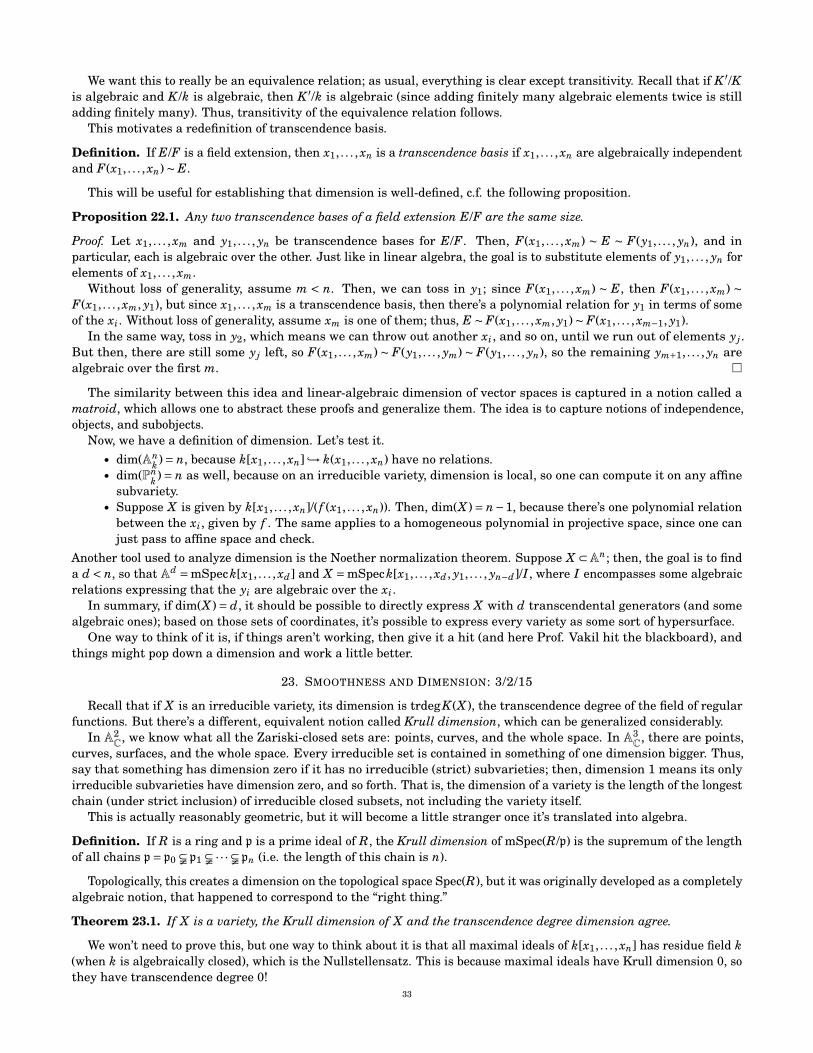
We want this to really be an equivalence relation; as usual, everything is clear except transitivity. Recall that if K ′/Kis algebraic and K /k is algebraic, then K ′/k is algebraic (since adding finitely many algebraic elements twice is stilladding finitely many). Thus, transitivity of the equivalence relation follows.

This motivates a redefinition of transcendence basis.

Definition. If E/F is a field extension, then x1, . . . , xn is a transcendence basis if x1, . . . , xn are algebraically independentand F(x1, . . . , xn)∼ E.

This will be useful for establishing that dimension is well-defined, c.f. the following proposition.

Proposition 22.1. Any two transcendence bases of a field extension E/F are the same size.

Proof. Let x1, . . . , xm and y1, . . . , yn be transcendence bases for E/F. Then, F(x1, . . . , xm) ∼ E ∼ F(y1, . . . , yn), and inparticular, each is algebraic over the other. Just like in linear algebra, the goal is to substitute elements of y1, . . . , yn forelements of x1, . . . , xm.

Without loss of generality, assume m < n. Then, we can toss in y1; since F(x1, . . . , xm) ∼ E, then F(x1, . . . , xm) ∼F(x1, . . . , xm, y1), but since x1, . . . , xm is a transcendence basis, then there’s a polynomial relation for y1 in terms of someof the xi. Without loss of generality, assume xm is one of them; thus, E ∼ F(x1, . . . , xm, y1)∼ F(x1, . . . , xm−1, y1).

In the same way, toss in y2, which means we can throw out another xi, and so on, until we run out of elements yj.But then, there are still some yj left, so F(x1, . . . , xm) ∼ F(y1, . . . , ym) ∼ F(y1, . . . , yn), so the remaining ym+1, . . . , yn arealgebraic over the first m. �

The similarity between this idea and linear-algebraic dimension of vector spaces is captured in a notion called amatroid, which allows one to abstract these proofs and generalize them. The idea is to capture notions of independence,objects, and subobjects.

Now, we have a definition of dimension. Let’s test it.• dim(An

k )= n, because k[x1, . . . , xn] ,→ k(x1, . . . , xn) have no relations.• dim(Pn

k )= n as well, because on an irreducible variety, dimension is local, so one can compute it on any affinesubvariety.

• Suppose X is given by k[x1, . . . , xn]/( f (x1, . . . , xn)). Then, dim(X )= n−1, because there’s one polynomial relationbetween the xi, given by f . The same applies to a homogeneous polynomial in projective space, since one canjust pass to affine space and check.

Another tool used to analyze dimension is the Noether normalization theorem. Suppose X ⊂An; then, the goal is to finda d < n, so that Ad =mSpeck[x1, . . . , xd] and X =mSpeck[x1, . . . , xd , y1, . . . , yn−d]/I, where I encompasses some algebraicrelations expressing that the yi are algebraic over the xi.

In summary, if dim(X )= d, it should be possible to directly express X with d transcendental generators (and somealgebraic ones); based on those sets of coordinates, it’s possible to express every variety as some sort of hypersurface.

One way to think of it is, if things aren’t working, then give it a hit (and here Prof. Vakil hit the blackboard), andthings might pop down a dimension and work a little better.

23. SMOOTHNESS AND DIMENSION: 3/2/15

Recall that if X is an irreducible variety, its dimension is trdegK(X ), the transcendence degree of the field of regularfunctions. But there’s a different, equivalent notion called Krull dimension, which can be generalized considerably.

In A2C, we know what all the Zariski-closed sets are: points, curves, and the whole space. In A3

C, there are points,curves, surfaces, and the whole space. Every irreducible set is contained in something of one dimension bigger. Thus,say that something has dimension zero if it has no irreducible (strict) subvarieties; then, dimension 1 means its onlyirreducible subvarieties have dimension zero, and so forth. That is, the dimension of a variety is the length of the longestchain (under strict inclusion) of irreducible closed subsets, not including the variety itself.

This is actually reasonably geometric, but it will become a little stranger once it’s translated into algebra.

Definition. If R is a ring and p is a prime ideal of R, the Krull dimension of mSpec(R/p) is the supremum of the lengthof all chains p= p0 á p1 á ·· · á pn (i.e. the length of this chain is n).

Topologically, this creates a dimension on the topological space Spec(R), but it was originally developed as a completelyalgebraic notion, that happened to correspond to the “right thing.”

Theorem 23.1. If X is a variety, the Krull dimension of X and the transcendence degree dimension agree.

We won’t need to prove this, but one way to think about it is that all maximal ideals of k[x1, . . . , xn] has residue field k(when k is algebraically closed), which is the Nullstellensatz. This is because maximal ideals have Krull dimension 0, sothey have transcendence degree 0!

33

Now, let’s calculate dim(Z). All prime ideals are of the form (0) or (p) for a prime p. If p and q are distinct primes,then p 6∈ (q) and vice versa, so the longest chain is (0)á (1). Thus, dim(Z)= 1.

What about Z[i]? Not all prime ideals lift from Z ,→Z[i]. For example, Z[i]/(5)=Z[x]/(x2 −1,5)= ((Z/5)[x]/(x−2))×((Z/5)[x]/(x+2)), but x2 +1 doesn’t factor mod 3, so (Z/3)[x]/(x2 +1)=F9, which is a field, rather than a product. But mod2, F2[x]/(x2 +1)=F2[x]/((x+1)2)=F2[t]/t2. This feels like a branched double cover, but in arithmetic! That is, it seemslike Spec(Z[i]) is a branched double cover of Spec(Z) — and it’s probably not a coincidence that each covering point iseither a field extension of order 2 (at (2) or (3 mod 4)), or a product of two field extensions of order 1, at (1 mod 4). Thisgets weird topologically, because it’s branched at exactly one point.

There’s a correspondence between Galois theory and that of covering spaces, and in fact one can use this to understandthe algebraic topology of Spec(Z)! For example, these correspondences can be used to show that there are no nontrivialconnected covering spaces, and therefore the universal cover is itself. Thus, π1(Spec(Z)) is trivial — Spec(Z) is simplyconnected. The correspondence is beautiful: topology turns into Galois theory, and vice versa.

Returning to varieties, let π : X →Y be a dominant (i.e. with dense image) map of irreducible algebraic varieties, i.e.K(X )/K(Y ) is a field extension.

Exercise 23.2. Suppose π : X →Y is a map of irreducible algebraic varieties and dim(X )< dim(Y ). Then, show that πis not dominant.

Solution. If this were dominant, then K(X )/K(Y ) would be a field extension with a smaller transcendence degree, whichcannot happen. �

If dim(X )= dim(Y ), then K(X )/K(Y ) is of transcendence degree zero, so it’s algebraic! Thus, we can talk about itsdegree (since all of these are finitely generated, then this extension is even finite algebraic).

Definition. Let X and Y be irreducible algebraic varieties of the same dimension. Then, the degree of a dominant mapπ : X →Y is deg(K(X )/K(Y )) (as a field extension).

In other words, a dominant map X →Y corresponds to an injective map K(Y ) ,→ K(X ).We can also talk about the codimension of a subvariety within another (which is the difference in their two dimensions).

If f is a function, what possible codimensions exist for spaces V ( f )? Clearly, if f = 0, we get a codimension 0 surface.If V ( f ) is irreducible, then it’s possible to show that it must have codimension 1! This can be proven geometrically oralgebraically (thanks to something called Krull’s principal ideal theorem). This was a little hand-wavy, but makes someintuitive sense, and can be made properly rigorous.

Claim. In P5, any five homogeneous equations of positive degree have a common, nontrivial solution.

Proof. Let’s look at A6 instead. Here, since the equations are homogeneous, the solution space includes 0. Then, it mustbe at least one-dimensional, if it is nonempty (by calculating the solution space of the first equation, then the second inthe first, and so on). But we have a solution, the origin! So the solution space is at least one-dimensional, so a solutionremains when we pass to projective space. �

Smoothness. We’ve already discussed smoothness here and there, implicitly. It’s yet another thing Brian Conrad putthe brakes on in a graduate-level class, so let’s talk about it.

We have, at least implicitly, the notion of the Zariski tangent space on a variety (or more generally, a scheme). IfX is affine and p ∈ X , then it corresponds to a maximal m within a ring R. Then, m is an R-module, so m/m2 is anR/m-module, i.e. a k-vector space. This is kind of weird, but has the right naturality properties to be the cotangentspace; thus, take its dual to obtain the tangent space.

This a priori seems like it would depend on coordinates, but when we localize, taking Rm and its maximal idealn=mRm, the result looks exactly the same: n/n2 =m/m2.

Well, what are the elements of this, actually? We have sets of open sets U and functions f on U , where ( f ,U)∼ (g,V )if there’s a neighborhood W of p such that W ⊂U ,V and f |W = g|W . In other words, one takes the direct limit as theopen neighborhoods get smaller and smaller, leading to the germs of functions at p, in some sense the local functions.This is a local ring, called Op, and its unique maximal ideal is the functions vanishing at p (since if you’re not in that,it’s possible to invert near p).

But this is also looks exactly like the definition of the tangent space to a manifold. A manifold, of course, is a ringedspace, and the tangents are germs of functions near a point p! So this is actually the same notion, and the direct limitand the sheaf was hiding there the whole time. This leads to forms in algebraic geometry.

So consider the following, uh, Math 51 problem: the surfaces x+ y+ x4 y7 = 0 and z+ (yxz)95 + x4 = 0 intersect at theorigin. What’s the tangent to this curve at the origin?

Instead of taking lots of derivatives and kvetching, we know m= (x, y, z), and m/m2 =αx+βy+γz for some α, β, andγ. But we can restrict the curves to m/m2: in particular, anything in m2 dies, including any higher powers. This equation

34

reduces to the much nicer x+ y = 0 and z = 0, and the linearization is exactly what they would get anyways. If thelinearization becomes 0= 0, then there is no nice tangent space (wrong dimension), which means it’s not smooth. Butit’s always true that dimk(m/m2)≤ dim(X ).

Exercise 23.3. Check that the integers are a smooth curve.

This is all really just calculus. Or maybe calculus is really just algebraic and differential geometry, which is whythese definitions seem to be the right ones.

24. THE TANGENT AND COTANGENT SPACES: 3/6/15

Today’s lecture was given by Donghai Pan.Assume k is an algebraically closed field and f (x, y) ∈ k[x, y]. Then, if f ∈ (x, y), then f (x, y)=αx+βy+·· · . Assume

at least one of α and β are nonzero; then, the curve corresponding to k[x, y]/( f ) is smooth at the origin (in the senseof taking partial derivatives, as well as the sense of algebraic geometry), and the tangent line is given by 0=αx+βy.Another way of saying this is that the tangent vector has the form t(β,−α) for t ∈ k.

Last time, we defined the cotangent vector space: if n denotes the maximal ideal (0,0)/( f ), then this is just n/n2. Thatis, n/n2 = (m/( f ))/(m/( f ))2 (where m= (0,0)), but this is just m/(m2 + ( f )) (the sum of modules given by taking sums ofgenerators of m and of ( f )). This can be viewed as the quotient space of m/m2 by ( f1), where f1 denotes the linear termof f . But this is therefore

{(u,v) |αu+βv = 0

}.

Since this is the cotangent space, the elements ought to be linear functionals, and the action is α(1,0) = 1 andα(0,1)= 0 (and then, since we need the sum to be zero, this defines how β acts). This means that we really get the linearfunctionals we were looking for, so this is in fact the cotangent space.

The next question is, how does the tangent vector come out of this? Recall that inside the ring k[x,ε]/(ε2), the mapx 7→ x+ε sends an f (x) ∈ k[x] to f (x)+ f ′(x) ·ε. Since this space contains information about the derivative of f , it’s usedto define tangent vectors, on varieties as well as on schemes.

The map k[x, y]/( f )→ k[ε]/(ε2) should be thought of as sending a point into the scheme k[ε]/(ε2) (it’s not nilpotent, soit’s not a variety!) that only has one maximal ideal (one point), but with some “fuzziness” which defines its direction.

Assume the preimage of (ε) is (x, y)/( f ), i.e. the point of k[ε]/(ε2) is sent to the origin. We could put this anywhere, sothe origin isn’t a bad choice, and it can be thought of as localizing at the origin. Then, x 7→ x0 + x1 ·ε and y 7→ y0 + y1 ·ε,with f (x, y)= 0 (mod ε2). But since the constant term is 0, then x0 = y0 = 0, so α · x1ε+β · y1ε= 0 implies αx1 +βy1 = 0.Thus, this seems like a reasonable notion of tangent direction.

Another way to look at this is that if A is a local ring, then Spec(k[ε]/(ε2))→Spec(A) gives all of the tangent vectorsof Spec(A) at the unique maximal ideal mA of A. The idea is, once we compute the corresponding map of rings, we getthe tangent space. But it seems like the key is not the global scheme, but some local data near it, so one can replacek[x, y] with k[x, y]( f ).

Smoothness. Related to this is the notion of smoothness.

Definition. Let A be a Noetherian local ring (e.g. k[x](x)), with maximal ideal m and residue field k = A/m. Then, A isregular (or is a regular local ring) if dimk(m/m2)= dim A (the latter as the Krull dimension).

If A is a finitely generated k-algebra, then one can use the transcendence degree dimension, but the Krull dimensionis more general.

The intuition is that regularity should be like a manifold: the dimension of a manifold, a property that can bedetermined locally (after all, it’s the dimension of the tangent space), is a global property. A regular ring has the sameproperty.

Example 24.1.• If k is a field, then it’s zero-dimensional as a finitely generated k-algebra (i.e. over itself), and (0) is a maximal

ideal, and dimk((0)/(0))= 0, so k is regular.• More interestingly, k[x](x) has two primes, (0)⊆ (x), and it’s regular and one-dimensional.• Z(p) is similar, with (0)⊆ (p).

Let p be prime; then, one can take the field extension Fp[x]/(xp −a) such that a doesn’t have a root in Fp. This is asomewhat funny thing, and will illustrate that regularity and smoothness aren’t the same thing; they are intuitivelysimilar for manifolds, and are indeed the same for perfect or algebraically closed fields, it’s not always the case. In otherwords, regular schemes and smooth schemes are not the same things.

Definition. Let k be an algebraically closed field and X ⊆Ank be an irreducible r-dimensional variety; then, an x ∈ X is

a non-singular point if the Jacobian matrix[∂ f i∂x j

]m×n

has rank n− r at x.35

Proposition 24.2 (Jacobian criterion). Let k be algebraically closed and X ⊆Ank be an irreducible variety. Then, X is

non-singular at an x ∈ X if Ox is a regular local ring.

Proof. Let I(X )= b⊆ k[x1, . . . , xn]. Then, an a ∈An corresponds to aa = (x1−a1, . . . , xn−an), so its image x ∈ X correspondsto mx ∈ k[x1, . . . , xn]/b.

Then, we want to show that aa/a2a∼= kn. Let θ : aa → kn send

f 7→⟨∂ f∂x1

(x), . . . ,∂ f∂xn

(x)⟩

.

Since X is non-singular, then θ is surjective.

Exercise 24.3. Show that ker(θ)= a2a.

Thus, θ : aa/a2a� kn is an isomorphism. (Alternatively, computing the dimensions, given that the map is surjective,

works too.) As before, mx/m2x can be identified with aa/(aa +b).

Now, what’s θ(b)? If b= ( f1, . . . , fn), then we’ll obtain ∇ f1, . . . ,∇ fn. These form into the matrix of partial derivatives (àla Math 51), and therefore the rank of the image spanned by these ∇ f i is equal to the rank of the derivative matrix.

If M′, N are submodules of a module M, if π : M�M′ is the canonical projection, then π(N)= (N +M′)/M′, which issimilar to the isomorphism theorems for rings. Thus, by checking the dimensions once again, b is sent to (b+a2)/a2.Specifically, this has dimension rank J, and ax/a2

x has dimension r. Then, mx/m2x = ax/(a2

x +b), which is a quotient of theother two modules, so its dimension is n− r. �

In other words, when k = k, regularity and smoothness are the same for affine varieties over k.This is still a fundamentally local idea; in general, all the calculations only care about the local rings. Thus, this

statement is also true for general varieties (e.g. projective varieties); the argument is in an affine neighborhood, andthat’s it.

Given an affine variety X , one can look at its singular locus. By thinking about determinants, this ends up beingequal to the set of x whose Jacobians have the property that all of their (n− r)× (n− r)-minors have determinant 0 at x.This is a finite condition (there are finitely many such minors) and the determinant is a polynomial condition, so thesingular locus is a closed subvariety of X .

25. IMAGES OF REGULAR MAPS: 3/9/15

Recall that a prevariety is a ringed space that locally is homeomorphic to mSpec(k[x1, . . . , xn]/I) (a nilpotent, finitelygenerated k-algebra), and, of course, k is algebraically closed. However, we forgot one important part of the definition:that it is required to be quasi-compact: every open cover has a finite subcover.

The first part says that it has a cover by affine spaces, and the second part means that it is covered by finitely manyaffines. This eliminates things such as infinite sets of points, etc.

Note that quasi-compactness sounds like compactness in other parts of mathematics; the difference is the Hausdorffcondition, which one does not require for varieties.

Let π : X →Y be a map of varieties. What can we say about π(X )⊂Y ? This relates to questions such as how oftentwo polynomial curves can intersect.

One might suspect that π(X ) is closed, but if X = k \ 0, Y = k, and π is inclusion, then the image is open but notclosed, and if X = {0} and π is inclusion, then the image is closed but not open, so we can’t say anything about whetherthey’re closed. The image might not even be a subvariety in some particularly weird cases. Moreover, any open or closedset could be the image of something (specifically, given by inclusion).

Well then, let’s talk about what (sub)sets can be the images of maps of varieties. This includes all open and all closedsets, but also unions, intersections, and complements of these sets.

Definition.• If X is a topological space, an A ⊆ X is locally closed if A = C∩U , where C is closed in X and U is open in X .• A subset A of a topological space X is constructible if it can be built from finite unions, intersection, and

complements, starting with open and closed sets.

Note that all open sets are locally closed.

Proposition 25.1. The constructible sets are exactly the finite unions of locally closed sets.

Theorem 25.2 (Chevalley). If π : X →Y is a morphism of varieties, then Im(π) is constructible.

This is actually quite powerful; thus (of course!) we will use it to prove the Nullstellensatz. As tends to happen inthis class, the theorem is true both for varieties and schemes, but the proofs differ.

Specifically, we will prove the most general version.36

Theorem 25.3 (Nullstellensatz, general version). Let k be any field and K /k be a field extension. Then, if K is finitelygenerated as an algebra, then it is a finite extension of fields.

Proof. If K isn’t a finite extension of fields, but is finitely generated as a k-algebra, then there exists an x ∈ K that istranscendental over k. Thus, k[x] ,→ K , so Speck[x]←SpecK , so mapping a point into an affine line, and we know whatthe points are.

In particular, we know the locally closed subsets of the affine line.

Exercise 25.4. Using the fact that A1k has the cofinite topology (as was on one of the homeworks), determine all of its

locally closed sets.

This can be used to embed Spec(K) into Spec(K[x]/I), for some ideal I. But this establishes an algebraic relation forx, which is a contradiction. �

The statement about the image being closed can be recovered in a different form. Specifically, using projective spacemakes things work better.

Proposition 25.5. The image of projection π :Pn ×Y →Y is closed.

Consider the following related problem. If we want to solve the following system of equations,

ax+by+ cz = 0

dx+ ey+ f z = 0

gx+hy+kz = 0

they constitute a curve in A9, but mapped from three curves in A3. This suggests that a constructive proof ofProposition 25.5 would provide a determinant. It’s also related to the question as to whether two polynomials share aroot, because each polynomial condition can be restated as projections from projective space.

Another result, called elimination of quantifiers, relates to interesting results in model theory and Banach’s realalgebras.

In P2, with coordinates x0, x1, and x2, consider four polynomials g1, . . . , g4. Then, do they have a common solution?(We’ll be able to do this for any values of 4 and 2.) It will turn out they do share a root iff they have a nontrivial solutionin A3 other than just 0, i.e. iff V (g1, . . . , g4) 6⊂V (x0, x1, x2), i.e.

√(g1, . . . , g4) 6⊇ (x0, x1, x2), i.e. (g1, . . . , g4)N 6⊇ (x0, x1, x2), or

for all N, (g1, . . . , g4) 6⊇ (xN0 , xN

1 , xN2 ) for all N, but this latter ideal is just that of degree-N homogeneous polynomials.

Then, we ran out of time, but this does lead down the right direction for this theorem (called the “fundamentaltheorem of elimination theory”): if Sm is the ideal of degree-m homogeneous polynomials, then there’s a map SN−deg(g1)⊕·· ·SN−deg(g4) → Sn (given by (·g1, . . . , ·g4)).

Now this is just a linear algebra problem, and the question boils down to determining whether a certain matrix issurjective. And we can do that using the determinant. This is a lot of things to check, in practice, but the point is we cando it.

26. THE FUNDAMENTAL THEOREM OF ELIMINATION THEORY: 3/11/15

Definition. If X and Y are topological spaces, a closed map is a continuous function f : X →Y such that the image ofevery closed set is closed.

Theorem 26.1. Let k be an algebraically closed field and Y be a variety. Then, π :Pn ×Y →Y is a closed map.

Proof. It suffices to do this in a local basis, since intersecting with an open set doesn’t change the condition. In particular,one can assume Y is affine, i.e. there’s a ring R such that Y = mSpec(R). In particular, these will be homogeneousequations with R-coefficients, and without loss of generality all of them have positive degree.

If R = k is a field, then this boils down to asking if a bunch of homogeneous polynomials g1, g2, . . . have a commonnontrivial solution in An+1 (equivalently, a solution in Pn).

We know V (g1, . . . )⊇ 0=V (x0, . . . , xn), i.e.√

(g1, . . . )⊆ (x0, . . . , xn) (since the latter ideal is already radical). Then, theyhave a common nontrivial solution if this inclusion is strict.

In particular, there’s no nontrivial solution if x0, . . . , xn ∈ √(g1, . . . ), and this is equivalent to xN

1 , . . . , xNn ∈ (g1, . . . )

for some N ∈ N. That is, SM , the Mth graded piece of the ring k[x1, . . . , xn] ⊂ (g1, . . . ) for some M (in the forwarddirection, M = N, but not necessarily in the reverse direction). That is, SM is equal to the Mth graded piece of (g1, . . . ),corresponding to a map SM−deg(g1)⊕SM−deg(g2)⊕·· ·→ SM that is not surjective (for all M, it’s not surjective). But this isequivalent to all of the maximal minors of the corresponding matrix being 0. This is a little strange to think about, butthis condition is polynomial, so the map is closed. �

Corollary 26.2. If Y is a variety and X ⊂Pn is a closed subset, then π : X ×Y →Y is also a closed map.37

We’ll be able to use this in many ways; for example, consider three conics; this triple of conics lives in Y =P5×P5×P5.Then, the points form a P2. The points that pass through all three conics form a closed condition, so one can applyCorollary 26.2 to get some conditions for the conics having an intersection.

The same story works for schemes, but some of the steps of the proof need to be different.

Upper Semicontinuity of Fiber Dimension. The preimage of a point (e.g. under Pn ×Y → Y ) is called a fiber,20 Iguess because it looks fibrous and is fun to say. The dimension of the fiber can vary, and we’ll see how that will affect thenumber of solutions.

Consider y= mx within A3, projected to the xy-plane. Most points have a single preimage, but the preimage of theorigin is an A1 (since if x = y = 0, then any m works). But we would like to work in P1, so instead we have ny = mx,which is homogeneous. Once again, the dimension only jumps up on closed sets, as any m and n work at the origin,giving a P1.

Remark. Let X ⊂ Pn be irreducible and have dimension d > 0. Then, every hyperplane meets X , but also there is ahyperplane not containing X , because the intersection of all of the hyperplanes is empty. Thus, a randomly chosenhyperplane will knock the dimension down by 1.

Definition. Let Z be a closed subset of Pn ×Y and π : Z →Y be the (restriction of the) canonical projection map. Then,the fiber dimension fd : Y →Z sends p 7→ dim(π−1(p)),21 with dim(;)=−1.

Theorem 26.3 (Upper semicontinuity of fiber dimension). fd−1([d,d+1, · · · ]) is closed.

Notice that the case d = 0 is Theorem 26.1.

Proof. As seen above, pick a hyperplane H, which intersects Z, so there’s a πH : Z∩H →Y . The image is a closed subset,and in particular, the intersections of the images for all of the hyperplanes is still a closed set.

For the more general case d, choose d intersecting hyperplanes. �

Theorem 26.4. Let π : X →Y be a regular map of varieties; then, fd : X →Z can be defined as p 7→ dim(π−1(π(p))), i.e.the largest dimension of the components of π−1(p). Then, this fd is also upper semicontinuous on X .

The trick in the proof is to restrict to a small open set (so we don’t have to worry about affine or projective or general),so that X ,→An ×Y π→Y , and Y is affine too, but we can take the compatification and use Pn in place of An. This doesn’tchange anything dimension-wise, since this is the closure, but allows Theorem 26.3 to imply upper semicontinuity on X .

This also works just fine for schemes.

27. CHEVALLEY’S THEOREM: 3/13/15

“I feel sorry for the scribes.”

Proposition 27.1. Suppose X and Y are irreducible varieties and ϕ : X → Y is a dominant map. Then, the fiberdimensions might jump, but we know that it’s upper semicontinuous. Then, it’s constant on some nonempty (and thereforedense) open set.

Proof. Without loss of generality, we can assume X and Y are affine, since we’re just looking for some open set, and canshrink as necessary.

Then, dim(X )= dim(Y )+dim(most fibers). There are two ways to prove this.• The first will use schemes, or I guess generic points, and is meant to illustrate how they can enrich the tools one

uses to prove things. Consider the generic points of X and Y ; the former must be sent to the latter, because ifnot, then the closure, i.e. X , is sent to some non-generic point, whose closure isn’t all of Y . We know the functionfield of Y , FF(Y ), has transcendence degree dim(Y ) over k (by definition), and FF(X ) has dimension r (whichis the dimension of fibers on some nonempty open) over FF(Y ), and dimension is additive, so we can expressdim(X )= dim(Y )+ r.

There’s lots to check here; specifically, some of the facts this proof leaned on require schemes, where weproved the results only for varieties. �

• There is a way to do this without generic points. Can you find it?

Theorem 27.2 (Chevalley). Let π : X → Y be a map of varieties. Then, π(X ) is constructible, i.e. it’s a finite union oflocally closed subsets.

20The British and French often prefer the alternate spelling fibre.21One thing to be careful of: dimension isn’t quite well-defined on open sets. So in this case, take the maximum over all compact subsets.

38

Proof. First, we can reduce to the case where X is irreducible; then, since all varieties are quasicompact, they havefinitely many irreducible components, and finite unions of finite unions remain finite. This means we can assume Yis irreducible as well, by just choosing the irreducible component of Y that π(X ) is contained into (since π(X ) is alsoirreducible, and therefore contained in an irreducible component of Y ). This means we can also assume Y is affine, andthat π is dominant, by working within the closure of π(X ).

Proposition 27.3. There is a dense open U ⊂Y such that π(X )∩U =U , or π(X )∩U =;.

Proof. Since π is dominant, then FF(Y ) ,→FF(X ) as fields; let r be the transcendence degree of this extension, so thatr ≥ 0.

We will reduce to the case when r = 0: if Y = mSpec(B) and X is given from B[x1, . . . , xn], then setting x1 = 0 is anontrivial equation which reduces the dimension by 1, since x1 is transcendent over Y . Then, pick an irreducible, affinecomponent of this set and continue. Repeating this over and over leads to the zero case, and if the n−1 case has a denseopen subset, then this will still be dense and open when considered within X , so the induction goes through.

Now, let’s talk about the base case, when r = 0. We can map X ,→ An ×Y → Y , so we can also map X ,→ Pn ×Y .Then, π(X ) is closed, and, since π is dominant, then the image is Y ! But since X is irreducible, then X \ X has smallerdimension than X (which has the same dimension as Y ), so the image can’t be all of Y ; instead, it’s a closed strict subset,and therefore the image of X contains a nonempty open. �

Now, since we’ve reduced to Y = π(X ), but if U =;, then its closure must be in the closed complement, which is afinite union of locally closed subsets (which requires a little more thinking). And if U ⊂π(X ), then we’re done. �

There’s a nicer way to deal with the inner proposition for generic points; specifically, the image of a generic point isgeneric, so the map in question is always dominant. Maybe this shines some light on why one would care about theseweird, fat points. Furthermore, in either case, dimension theory and upper semicontinuity also have to come together tomake the proof happen.

Retrospective. Well, that was an insane idea realized: teaching algebraic geometry to undergraduates. What all havewe done?

• Polynomials and the curves they cut out in kn.• Homogeneous polynomials in Pn

k , and that Aut(Pn)=PGL(n+1). Linear polynomials in projective space. Bézout’stheorem.

• Higher-degree polynomials, where it’s useful to have k algebraically closed. As a particular case, conics (degree-2): their classification, as long as k is algebraically closed. In degree-3 cubics, we talked about the group law(though we never did prove associativity. . . ), and their Weierstrass normal forms, so long as they had a flexpoint.

• This group law makes a lot more sense if we had topology, e.g. over C. But more generally, we have the Zariskitopology, which began with vanishing sets V (I)⊂An, the closed sets of a weird and wild topology. This leads toNoetherian rings, with the consequences that infinitely many equations on An are the same as finitely many,and that every affine variety has finitely many irreducible components. In the other direction, we have I(S), sothat V (I(S))= S and I(V (J))=p

J, which is the Nullstellensatz! Moreover, all affine varieties are quasicompact.(This is already well over a quarter’s work, but we were just a few weeks in!)

• Affine varieties, with their maps X →Y , form a category. So do affine schemes (just for fun).• The relation between rational functions and regular functions, relating to localization in algebra; domains

of definition, which are big (i.e. nonempty) open sets. We saw birational maps between algebraic varieties;whenever we can easily solve a Diophantine equation, it was birational to An, but there are cubics that aren’tbirational, and therefore are somewhat harder to solve.

• We defined varieties, and prevarieties; this involved talking about sheaves, including the sheaf of regularfunctions on (irreducible) affine varieties. Then, varieties are given by quasicompact locally ringed spaces (sowith the sheaf of functions) which locally look like affine varieties. This allows one to define manifolds, products,Hausdorff spaces, projective varieties, and so forth.

If you’re keeping track, this is a second quarter’s worth of stuff.• Dimension theory! The transcendence degree and Krull dimensions agree in the cases we care about, and the

definition of smoothness and the Zariski cotangent space, which are a sort of calculus. A nontrivial equationcuts the dimension down by one.

• The fundamental theorem of elimination theory, upper semicontinuity of dimension, and Chevalley’s theorem.I think that makes for a third quarter of content. How wonderfully insane. The writing projects will add at least aquarter’s more worth of material.

39