DISCUSSION PAPER SERIES DPS13.07 APRIL 2013

Maternal employment: the impact of triple rationing in childcare in Flanders Dieter VANDELANNOOTE, Pieter VANLEENHOVE, André DECOSTER, Joris GHYSELS and Gerlinde VERBIST

Public Economics

Faculty of Economics And Business

Maternal employment: the impact of triple rationing inchildcare in Flanders∗

Dieter Vandelannoote†, Pieter Vanleenhove‡,André Decoster‡, Joris Ghysels§, Gerlinde Verbist†

19th April 2013

Abstract

This paper analyses how maternal labor supply responds to the price and availab-ility of childcare services. It focuses in particular on the childcare market of Flanders,which is characterised by above average childcare use, a wide variety of price schemesand suppliers, and strong government supervision regarding quality.

Variation in prices and the degree of rationing of three types of childcare servicesat the municipal level are used to identify mothers’ labor supply responses. A discretelabor supply model of the Van Soest (1995) type is elaborated to allow for heterogen-eity in prices and to distinguish between rationed and non-rationed households.Theseextensions rest on rationing probabilities that are estimated separately for informalchildcare, formal subsidised childcare and formal non-subsidised childcare using par-tial observability models (Poirier,1980).

The estimates confirm earlier findings for Germany and Italy, indicating only smallprice effects and relatively large supply effects. This shows that labor supply incentivesof expansion of childcare services are also present in a country which has surpassed theEU target of childcare slots for 33% of children below the age of 3 (Belgium, in contrastwith Germany and Italy). Moreover, budgetary simulations suggest the expansion tobe beneficial to the exchequer. Rising tax and social security benefits following theincrease in labor supply largely exceed the costs of expansion.

JEL Classification: C35 H24 J13 J22 D10Keywords: Labor supply, Childcare, Microsimulation

∗We are grateful to the participants of the IMPROVE workshop at CHILD in Turin, 1 October 2012, ofthe Microsimulation research workshop in Bucharest, 11-12 October 2012 and of the PE-ETE seminar inLeuven, 15 November 2012. The usual disclaimer applies.†Centre for Social Policy Herman Deleeck, University of Antwerp‡Centre for Economic Studies, KU Leuven§TIER, University of Maastricht

1

1 Introduction

Childcare is a key factor in the employment decisions of parents, especially of mothers.The availability of different childcare options, their quality and their price are major de-terminants of the work-family balance of households with (young) children. These issuesfigure also highly on the policy agenda, which is illustrated by the Europe 2020 target ofincreasing employment rates toward 2020 to 75% for the population aged between 20 and64. Especially for women there is scope to increase the employment rate, and formal child-care provisions figure prominently among the policy instruments to achieve this goal.1 TheBarcelona childcare targets formulated in 2002 by the European Council, and confirmed in2005, should be viewed as part of this framework.2

In this paper we investigate the effect of different childcare options in terms of availabilityand prices on employment decisions of mothers with young children in Flanders (Belgium).The case of Flanders and/or Belgium in this domain remains largely under-studied, eventhough the childcare context is interesting from an internationally comparative viewpoint.To some extent, the Belgian welfare state remains oriented towards the breadwinner model(e.g. in the form of substantial derived social security rights, tax support for sole earners).However, in contrast to other continental welfare states, such as Germany, Belgium com-bines this with a well-organized and more wide-spread system of institutional childcare,and can thus be characterized by what Leitner (2005) called ‘optional familialism’. Withan enrolment rate in formal care of children younger than three of 48.4% (2008), Belgiumfigures among the top nations in this respect in the OECD.3

Nevertheless, this does not mean that availability of childcare places is not an issue inBelgium. There are indications that all three forms of non-parental childcare that we distin-guish (i.e. informal care, non-subsidized and subsidized formal care types) are characterizedby excess demand, and hence that rationing is at work in the three types. The richnessof our dataset, the Flemish Families and Care Survey, allows us to incorporate this triplerationing in our empirical analysis, which is a novelty in the literature. The distinctionbetween types allows for a robust identification of price and availability (supply) effects,since the price and supply of the types varies strongly between municipalities, while theservice quality is relatively homogeneous, because public supervision extends to all typesof (formal) childcare.

Our paper builds on a structural labor supply model as proposed by Van Soest (1995),using a discrete random utility maximization model. We extend this framework by explicitlytaking triple rationing in the Flemish childcare market into account. We do so in two ways.First, in line with Wrohlich (2011), access restrictions to childcare are taken into account in

1According to EUROSTAT, the employment rate for men in the EU in 2010, the year when Europe 2020was launched, was 75.1% while for women it was 62.1%.

2According to these targets, each country should provide childcare by 2010 to at least 90% of childrenbetween 3 years old and the mandatory school age and at least 33% of children under 3 years of age.

3Only the Nordic States and the Netherlands have higher rates. (OECD, 2011).

2

the budget constraint of each household. The expected price households pay for childcaredepends on household-specific offer probabilities of each type of care. Households whoenjoy a large probability of being offered a childcare spot of the informal type have a lowerexpected childcare cost than a similar household with a low offer probability of informal care.These offer probabilities are estimated by applying the partial observability framework, assuggested by Poirier (1980). In contrast to Wrohlich (2011), we also take rationing in theformal non-subsidized childcare sector into account, as we have clear evidence that thissector also faces excess demand. Second, in the estimation of the labor supply model wemake a distinction between two different groups of households depending on their access tochildcare. Households that have a low probability of finding suitable childcare in generalare assumed to face a restricted labor supply choice set.

This paper contributes to the existing literature in several ways. First, because we haveclear evidence that the non-subsidized childcare sector in Flanders faces excess demand, weextend the framework suggested by Wrohlich (2011) and explicitly take this rationing intoaccount in the model. Thus, we no longer rely on an automatic market clearing assump-tion to identify rationing effects. Second, we propose an alternative way of taking totalrationing in the childcare market into account in the estimation of the labor supply modelby distinguishing between two groups of households, i.e. the non-restricted and restrictedhouseholds. Households who face a low probability of finding suitable childcare, face arestricted labor supply choice set. Finally, our methodology can be used to analyse howlabor supply is affected by different policy changes. In line with estimates from countrieswith stronger supply restrictions (Italy and Germany), we find that, for a country with arelatively generous service supply, maternal labor supply is more sensitive to changes inthe availability of care than to changes in price. Not surprisingly, the estimates of the netbudgetary effect of expansion plans are strongly positive.

The paper is organized as follows. Section 2 discusses the childcare context in Flanders.Section 2 gives a brief overview of related studies in the literature. Section 4 explains indetail how the different offer probabilities for the three types of childcare are estimated byapplying the partial observability model suggested by Poirier (1980). Section 5 presents ourmethodological framework, and the data assumptions are explained in Section 6. The laborsupply estimation results and labor supply impact of some alternative policy scenarios arepresented in Section 7. The final section concludes.

3

2 Childcare in Flanders

This section discusses the childcare context in Belgium and more specifically in Flanders.Section 2.1 gives an overview of which categories of care can be distinguished and howfrequently they are used. Section 2.2 discusses in further detail three important elementsof the childcare market in Flanders: the price, the quality, and the availability of childcare.

2.1 Types and usage of childcare

The childcare landscape in Belgium, and more specifically in Flanders, is highly fragmen-ted, as can be seen in Table (1), but can roughly be divided in two categories: formaland informal care. Child and Family (Kind en Gezin, K&G) supervises the organizationof formal childcare in Flanders and controls whether childcare providers meet the legalrequirements.4 Formal childcare mainly focuses on children between 3 (end of maternityleave) and 30 months (start of publicly-financed nursery school).

A closer look at formal childcare providers suggests a distinction between subsidized andnon-subsidized care. The former receives cost-covering subsidies from Child and Family,for which they need to be accredited. The formal non-subsidized childcare providers arenot eligible for these subsidies, and need only to register.5 In both cases, parents canapply for a tax deduction, which is not the case if providers do not register. Therefore,client pressure may explain why almost all formal care providers (both subsidized and non-subsidized) are registered, and thus controlled by Child and Family. Secondly, in bothsubsidized and non-subsidized care, a distinction can be made between child-minders andday nurseries. Child-minders take care of a relatively small group (max. 8) of childrenin their own house, whereas day nurseries are located in specific childcare centres. Thereare also local services for neighbourhood-oriented care that are small childcare initiativesaimed at providing diverse and easily accessible childcare, especially for more vulnerablefamilies.6 Child and Family partly subsidizes the latter initiatives working towards equalopportunities (Ghysels and Vercammen (2012) & Kind en Gezin (2012)).

Beside formal childcare, informal childcare is also an important care channel. Mainlygrandparents, but also other family members, neighbours, or friends are possible providersof care.

User surveys reported in Bettens et al (2002) and Hedebouw and Peetermans (2009b),reveal a strong increase in the the frequent use of childcare (from 49% in 2001 to 63% in

4The same is undertaken by the Bureau of Birth and Childhood (Office de la Naissance et de l’Enfance,ONE) in the French speaking community.)

5In order to be accredited, childcare facilities need to fulfil different legal requirements, which is not thecase if you are only registered.

6The first initiatives of local services for neighbourhood oriented care were taken in 1998 in Brussels,Antwerp and Leuven. They received project-based support from Child and Family. Since 2009, this typeof childcare is legally and structurally integrated into the Flemish childcare landscape. More informationcan be found at: http://www.lokalediensteneconomie.be/node/9.

4

2009).7 The percentage of families that never used any type of childcare gradually decreasedfrom 41% in 2001 to 31% in 2009. Table (1) looks at the evolution of the main childcarechoices amongst families in Flanders. The use of informal care as the primary care-takingchannel decreased in favor of formal care (mainly the non-subsidized part of it). Withinthe non-subsidized formal care sector, the most notable rise regards the (near) doubling ofchild minders as the primary care-taking channel between 2001 and 2009.

Table 1: Most frequently used type of childcare, 3 months – 3 years, Flanders (%).

2001 2009Formal subsidized care 45.6 46.9- Child-minders 28.7 28.5- Day nurseries 16.9 18.4Formal non-subsidized care 17.8 23.9- Child-minders 9.6 17.6- Day nurseries 8.2 6.3Informal care (grandparents) 29.9 22.4Source: Bettens et al (2002) and Hedebouw and Peetermans (2009b)

2.2 Price, quality and availability of childcare

The price, quality and availability are three central factors of the market for childcareservices. This section discusses each of these items in detail for the Flemish childcarecontext.

2.2.1 The price of childcare in Flanders

A first important aspect of childcare relates to the price paid by parents. This price differsaccording to the type and amount of care.

Subsidized providers of formal childcare are obliged to apply a legally determined means-tested tariff structure, dependent on household income. The payment rate differs in blocks,rather than hourly proportions.8 In 2005, which is the year of the survey used in this paper,78% of the children who were in formal subsidized childcare stayed a whole day (between 5and 12 hours) and paid 100% of the daily price. This daily price lies between a minimumprice of 1.28 Euro and a maximum of 22.82 Euro with an average cost of 13.5 Euro. Adiscount of 2.58 Euro is given for each dependent child in the family, after the first, and formultiples.9 Childcare providers can also freely choose to apply a social tariff for households

7The category ’frequently’ means minimum 5 hours of childcare per week. For preschool children, these5 hours need to take place in a continuous period. For children between 2,5 and 3 years going to a nurseryschool, this continuity is not necessary.

8Four different categories can be distinguished. A Mini Day amounts to [0,3[ hours of care/day and ischarged 40% of the daily cost. A Half Day reflects [3,5[ hours/day and is charged 60% of the daily cost. AWhole Day is equal to the range of [5,12[ hours/day and is charged at 100% of the daily price and a MaxiDay reflects [12,24[ hours/day and costs 160% of the daily cost.

9For 2012, the minimum daily price is 1.5 Euro, the maximum price 26.68 Euro and the average dailycost is 13.7 Euro. A discount of 3.02 Euro is given for each dependent child in the family.

5

in a financially difficult situation, which is either 75, 50 or 25% of the normal means-testedtariff.10

Non-subsidized providers of formal childcare are free to determine the price they charge.Not much information is available about the price setting by these providers. The bestsource available is a Child and Family report from 2009 (Hedebouw and Peetermans,2009a). Based on this report, we can determine the average daily cost for a whole dayin non-subsidized care for children between 0 and 3 years old in Flanders. On average, anon-subsidized child minder charges 17.16 Euro in 2009 and a non-subsidized day nursery21.16 Euro. Reacting upon concern about the growing market share of the non-subsidizedsector (see Table (1)), and hence the expected growing cost for low income families, theFlemish government introduced, as a test case, in 2009 the means-tested tariff system inthe non-subsidized sector. Registered but non-subsidized facilities may opt to join thesystem wherein the same means-tested tariff structure as in the subsidized sector is ap-plied. The Flemish government complements the parent’s means-tested contribution up toa guaranteed daily price. 11 (Ghysels and Vercammen (2012)).

Additionally, parents who use accredited childcare (both formal subsidized and non-subsidized) are eligible for a tax deduction. The taxable income of the fiscal unit is reducedwith out-of-pocket costs of childcare service, with a maximum of 11.20 Euro per day perchild in care. Since 2005, this is possible for dependent children until the age of 12. Familieswho do not deduct childcare fees qualify for a lump sum raise of the income tax exemption,equal to 520 Euro for every child younger than 3 in 2012 (Ghysels et al (2010)).

No information about prices (parental costs) in the informal sector is available. In theempirical part of this paper, we assume that the cost paid by the parents for informalchildcare equals zero, which is the common assumption in the literature.

2.2.2 The quality of Flemish childcare facilities

A second important element is the quality of the care provided by the different child carefacilities. Both formal subsidized and non-subsidized childcare meet the legal requirementsof quality care, as determined by Child and Family. However, this doesn’t guarantee apermanent level of high quality in itself. A quality check is only done at the opening ofa care center or when deemed necessary (e.g. after several complaints). The caretaker istherefore itself responsible for the level of quality provided. Yet, this structural commentdoes not obviate that satisfaction among parents is very high. A survey conducted byChild and Family in 2009 (Hedebouw and Peetermans (2009a)) gives an idea about thequality of childcare as perceived by parents in Flanders with a child between 0-3 years old.96.2% judge the quality of the main care taking channel as very good (64.2%) or good

10No information about the frequency of use of this social tariff is available.11Within the simulations presented in this paper, we use data from 2005. This means that we don’t use

the means-tested tariff structure for the non-subsidized childcare sector, because this was first implementedin 2009.

6

(32%). Informal care (mainly grandparents) is perceived as the most qualitative form ofcare. Formal non-subsidized is considered the least qualitative one, although still more than95% of the users judge this type of care as very good (55.9%) or good (39.4%). Questionsabout the well being of the child in childcare gave similar results.

2.2.3 Triple rationing in the Flemish childcare market

A final important element regards the availability of childcare. There are indications thatall sorts of childcare services are in short supply in Flanders. Research commissioned byChild and Family in 2007 indicated that 10% of parents were not able to secure a suitablechildcare service after a search period of six months (Market Analysis and Synthesis (2007)).Obviously, we acknowledge that a cross-section result based on those who are currently inthe market does not provide full information on the dynamics of demand and supply. Ineffect, supply may expand in the medium term and excess demand may be eliminated bymarket forces. Haan and Wrohlich (2011) assume in their analysis of labor and childcare inGermany, for example, that market forces automatically clear the market through supplyby non-subsidized providers. In their approach, rationing is limited to supply of subsidizedand informal care, which does not respond to classic market dynamics (e.g. rising prices).

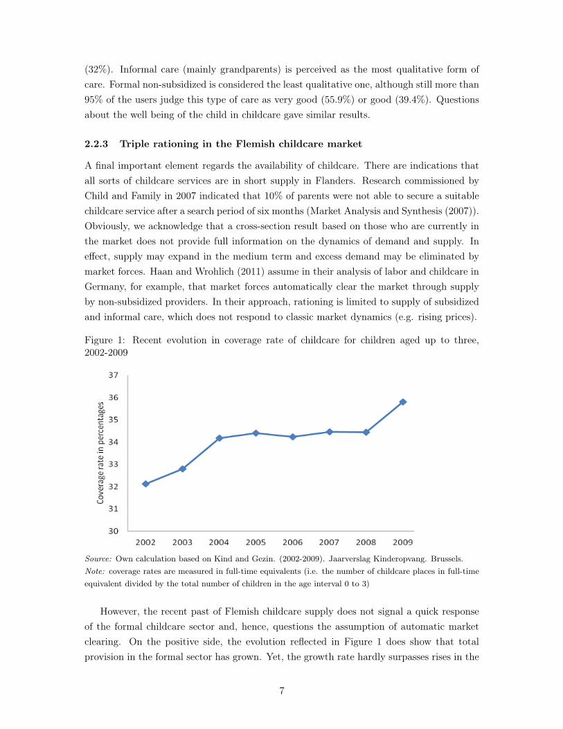
Figure 1: Recent evolution in coverage rate of childcare for children aged up to three,2002-2009

Source: Own calculation based on Kind and Gezin. (2002-2009). Jaarverslag Kinderopvang. Brussels.Note: coverage rates are measured in full-time equivalents (i.e. the number of childcare places in full-timeequivalent divided by the total number of children in the age interval 0 to 3)

However, the recent past of Flemish childcare supply does not signal a quick responseof the formal childcare sector and, hence, questions the assumption of automatic marketclearing. On the positive side, the evolution reflected in Figure 1 does show that totalprovision in the formal sector has grown. Yet, the growth rate hardly surpasses rises in the

7

birth rate, and does not account for growing employment rates among mothers. Knowingconcurrently that informal (grandparental) care is on the decline (Ghysels and Van Vlas-selaer (2007)), it is clear that over the last decade overall excess demand (formal+informal)has not been eliminated.

Our second observation relates to the composition of the Flemish childcare servicesmarket, which suggests a three-leveled hierarchy of rationing. Rationing that most parentsare likely to be confronted with, stems from the changing role of grandparents. As inmost European countries (Hank and Buber(2009)), the care contribution of grandparents isdecreasing in Flanders. Several explanations are given, such as more active ageing, throughwhich grandparents are still working or do not have the time to take care of children.Meanwhile, many parents state that grandparents are their preferred care providers (Ghyselsand Debacker (2007)), which should not come as a surprise given their traditional role inchild-raising and the fact that they usually do not charge a price for their help.

Yet, childcare rationing goes beyond the informal part. Development of subsidized andnon-subsidized formal childcare led to locally uneven results. Municipal supply statisticscorresponding to our period of analysis (December 2004) show that the coverage rate12

of subsidized childcare averaged 24% and the coverage rate of non-subsidized childcareaveraged 11%. 13 For formal childcare overall, Flanders, 340 municipalities had an averagecoverage rate of 34% (interquartile range 27 to 40%). While one small municipality boasteda coverage rate of over 100%, it is more important to observe that the 95th percentile’scoverage rate is only 54%. Confronted with municipal employment rates of mothers withyoung children of on average 70%, there is little doubt that rationing in both the subsidizedand the non-subsidized childcare sectors may exist in at least some locations.14 Therefore,we will assume that besides grandparental rationing, parents can also experience rationingin subsidized and non-subsidized formal childcare.

12The coverage rate is defined as the amount of slots as a percentage of children below the age of 3 livingin the municipality.

13The interquartile range for the former equals 27% to 40% and for the latter 3% to 16%.14Note that the part-time nature of demand for childcare does not warrant a simple equation of the

coverage rate with the employment rate of mothers. In effect, a full-time childcare slot may cover for morethan one child. As a rule of thumb, the Flemish childcare authority ‘Kind en Gezin’ assumes in its planningexercises that a full-time slot can cover the demand of 1.2 children.

8

3 Literature review

There exists a large amount of literature describing the effect of children, and more specific-ally the effect of childcare, on parental labor supply. Anderson and Levine (1999), Brewerand Paull (2004) and Kalb (2009) provide overviews of the existing studies related to child-care and labor supply. This latter study discusses in detail how the cost, availability andquality of childcare affect parental labor supply decisions for different countries.

The literature about labor supply and childcare demand can be broadly classified intotwo categories depending on the assumptions made regarding parental demand for childcare.The first stream considers childcare as a way to make time time available for parents toengage in market work. As such, childcare only forms part of the cost of working andthe demand for care is completely determined by the parental labor supply decision. Thisis known in the literature as the “Cost of Working” approach, and only the employmentdecision is endogenously modelled. Kimmel (1995), Averett et al (1997) andWrohlich (2004)are examples of studies that can be found in this stream of literature. The second streamassumes that households make their employment and childcare decisions simultaneously,and thus it is known as the “Simultaneous” approach. Examples of studies that work inthe “Simultaneous” approach are Connely (1992) and Ribar (1995) for the United Statesand Kornstad and Thoresen (2007) for Norway.15 The work presented in this paper canbe situated in the first stream of literature as our main purpose is to see how employmentdecisions are affected by characteristics of the childcare market and not how childcarechoices are made.

The existing literature focuses mainly on three aspects of childcare: price, quality andavailability. Basic economic intuition suggests the price of childcare to be one of the mostimportant features of childcare in the parental labor supply decision. Hence, many studies,regardless of working with a “Cost of Working” or “Simultaneous” approach, have put em-phasis on these costs to explain labor market behaviour, such as the participation decisionof mothers. These effects are most often presented as elasticities that report the percent-age change of labor supply and labor market participation which results from a percentagechange in childcare prices. Anderson and Levine (1999), Brewer and Paull (2004), Kalb(2009) and Gong, Breunig and King (2010) provide summary tables of estimated elasti-cities for different countries and subgroups. Their estimates vary across a wide range butindicate that, on average, childcare prices affect labor supply negatively. For example, Blauand Robins (1988) find for the United States an elasticity of maternal employment relativeto the price of childcare of -0.34; Ribar (1995) reports an elasticity of -0.09 for marriedwomen in the United States; and Wrohlich (2004) finds an elasticity of -0.21 for Germanmothers with full-time working husbands. Gong, Breunig and King (2010) state that thisvariation partly reflects the fact that childcare and other welfare institutions vary acrosscountries and that differences in methodology and data sources may also play an important

15For a more detailed overview, see Brewer and Paull (2004) and Kalb (2009)

9

role, making a direct comparison difficult. Anderson and Levine (1999) find that paperstaking a structural approach obtain elasticities on the lower end of these estimates, rangingbetween 0 and -0.1.

In more recent literature, the focus has shifted from the cost of childcare to its avail-ability and accessibility. This literature provides mixed evidence of the size and sign ofthe effect of these availability constraints on labor supply. For Germany, Hank and Krey-enfeld (2000) employ a multinomial logit model to estimate how the availability of publicand informal day-care arrangements affect female labor-force participation. The authorsfind no significant effect of regional childcare provision on female labor-force participation.Wrohlich (2011), however, does find significant labor supply responses for German moth-ers of an increase in childcare availability. Wrohlich (2011) models availability restrictionsexplicitly in the budget constraint, and assumes that rationing occurs only with respect tosubsidized childcare. The author assumes that childcare can always be bought at some (po-tentially very high) price on the private market. Wrohlich (2011) shows that policy reformsin Germany targeted at an increase in childcare slots had larger effects on maternal laborsupply than reductions of the cost in childcare. For Italy, Del Boca (2002), Del Boca andVuri (2007) and Brilli et al. (2011) find a positive impact of childcare availability on thelikelihood of mothers working. These studies restrict the choice set of households accordingto a simulated probability of being rationed in the childcare sector. For Russia, Lokshin(2004) models rationing by restricting the choice set of parents who report to be rationed inthe childcare market. Kornstad and Thoresen (2007) follow a similar method for Norway.Both studies find positive labor supply responses to increased availability of the childcaresector.

For Belgium in particular, there is hardly any literature about the effects of childcareon labor supply decision of households. The only recent paper that estimates labor supplyelasticities with respect to childcare costs is Van Klaveren and Ghysels (2012). The authorsfind, in contrast to many studies in the literature, positive labor supply elasticities withrespect to childcare costs. However, it is hard to compare their work to the work presentedin this paper because the authors use a collective household model which treats childcarecosts as a pure income effect, given the power balance (sharing rule) in the household.Rising costs reduce the non-labor income of the household and, hence, motivate parents toincrease their working hours. Farfan-Portet, Lorant and Petrella (2011) analyse the impactof both demand-side and supply-side subsidies on the use of formal childcare by low incomefamilies in Belgium. They conclude that the choice of policy instruments is not neutral interms of access to formal childcare for families of different income groups. As such, theauthors call for a heterogenous treatment of rationing and availability restrictions, takinghousehold characteristics into account. We will return to this issue below.

10

4 Triple rationing in the childcare sector

This section discusses in detail how rationing in the childcare sector is accounted for. Giventhe triple face of rationing, we look in detail at the search process of parents when lookingfor a suitable childcare place and estimate the probability of them being rationed in theirchildcare choice.16

4.1 Rationing and the stepwise search for a childcare slot

Earlier, we characterized the Flemish childcare market and described its three main typesof care. In this section we develop an ordered estimation strategy based on the priceand quality attributes of the three types of care, which suggests a rationing hierarchy.Grandparents hardly ever charge for their care, which makes their care by far the most cost-attractive for parents. Even if opinions on the inherent quality of grandparents as carersmay differ between parents, we assume the price element to trump potential preferenceissues and, hence, assume that parents who are looking for childcare will first turn to thegrandparents if available.17 Only if they cannot assure grandparental care to cover theirfull care needs, parents will start searching within the formal sector.

Within the Flemish formal childcare sector, prices can be treated as the dominantfactor. The regulatory framework ensures that all types of providers attain high qualitylevels, but prices vary strongly.18 In the subsidized sector, parents pay an income-relatedfee with a maximum of e25 per day, while non-subsidized providers are free to determinetheir prices. Even though a survey amongst non-subsidized providers of childcare servicesin 2008 suggested that hardly any of them charge a daily price over the maximum of thesubsidized tariff 19, their prices are not income-related and, hence, using childcare in thenon-subsidized sector results in considerably higher costs than in the subsidized sector formost parents.20 Therefore, we assume the non-subsidized sector to be the provider of lastresort, when parents cannot cover their care needs with grandparental help nor with carefrom a subsidized care provider.

In short, we assume the search process of parents to follow the cost hierarchy of childcareservices in Flanders: first grandparents are considered as childcare providers, then an offerof subsidized childcare is looked for and lastly parents attain whether they can secure a slotin the more expensive non-subsidized sector.

16Note that we do not make a distinction between rationing for childminders and day nurseries. We onlyfocus on the distinction between informal, formal subsidized care and formal non-subsidized care.

17Ghysels and Debacker (2007) show that grandparental care is the most preferred type of childcare. Seealso section 2.2

18Non-accredited providers are believed to be of marginal importance. (Kind en Gezin 2010)19Unpublished data obtained from the Flemish governing authority ‘Kind en Gezin’.20Earlier calculations by the authors indicate that even in the ninth income decile the income-related fee

amounts to less than 20 Euros a day, a 20% discount with regard to the usual price in the formal sector(childcare centres).

11

4.2 Rationing estimation through partial observability models

As will be discussed in the following section, our labor supply model incorporates estim-ates of the offer probabilities of childcare that parents experience. The model necessitateshousehold-specific offer probabilities of childcare in general and for each type of care indi-vidually. The general offer probability will be used to determine the set of labor marketchoices that are open to specific parents, while the offer probabilities of each type will becombined into a household-specific price of childcare.

Therefore, we estimate four offer probabilities: total supply (any type of childcare),supply in the subsidized sector, supply in the non-subsidized sector and supply of informalcare (grandparental care).

To estimate these supply probabilities, we rely on a simultaneous estimate of demandand supply of childcare using the partial observability probit framework suggested by Poirier(1980) and adapted to a childcare setting by Viitanen and Chevalier (2003). We do notapply the modified framework suggested by Wrohlich (2008), because, unlike Germany,we see no large group of municipalities with full coverage, as already documented above.The historically high supply of childcare services in the eastern part of Germany allowedWrohlich (2008) to restrict estimation to demand for only part of her sample, but no suchsituation exists in Flanders.21

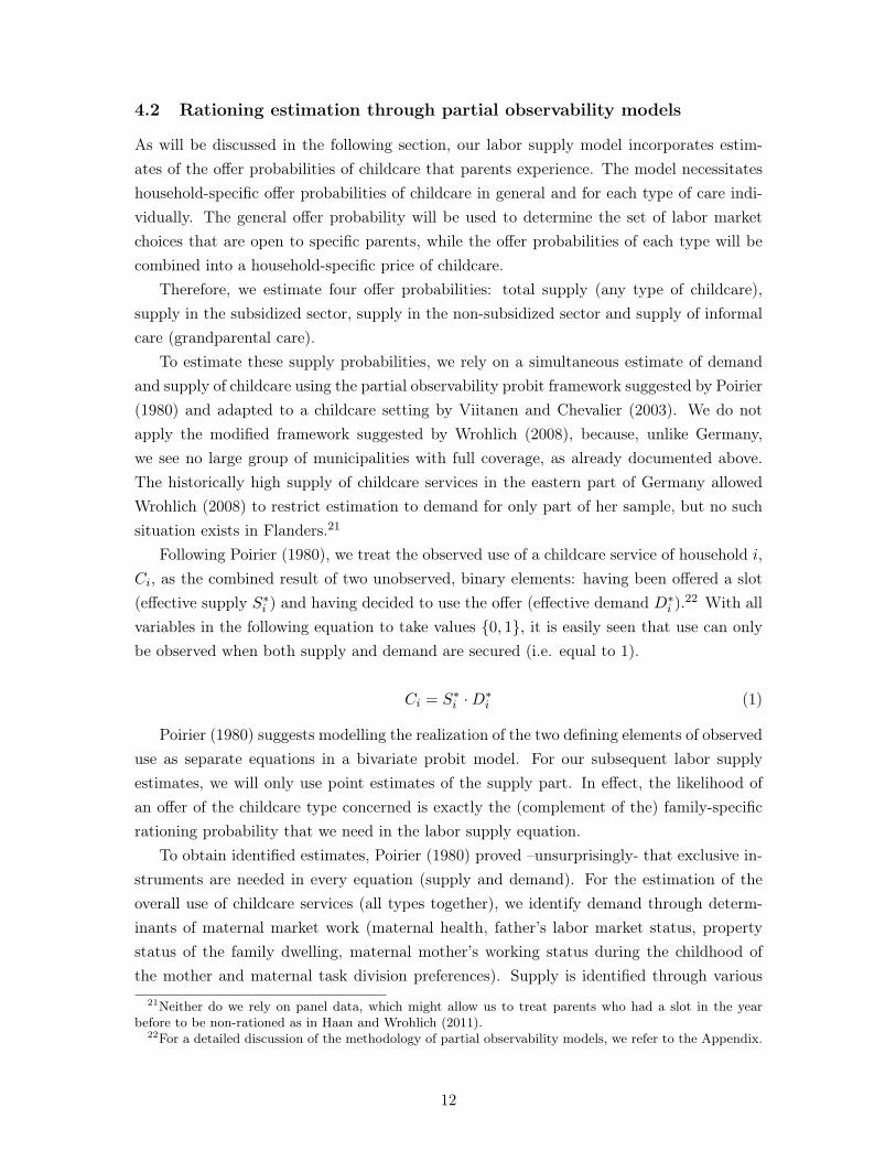
Following Poirier (1980), we treat the observed use of a childcare service of household i,Ci, as the combined result of two unobserved, binary elements: having been offered a slot(effective supply S∗i ) and having decided to use the offer (effective demand D∗i ).22 With allvariables in the following equation to take values {0, 1}, it is easily seen that use can onlybe observed when both supply and demand are secured (i.e. equal to 1).

Ci = S∗i ·D∗i (1)

Poirier (1980) suggests modelling the realization of the two defining elements of observeduse as separate equations in a bivariate probit model. For our subsequent labor supplyestimates, we will only use point estimates of the supply part. In effect, the likelihood ofan offer of the childcare type concerned is exactly the (complement of the) family-specificrationing probability that we need in the labor supply equation.

To obtain identified estimates, Poirier (1980) proved –unsurprisingly- that exclusive in-struments are needed in every equation (supply and demand). For the estimation of theoverall use of childcare services (all types together), we identify demand through determ-inants of maternal market work (maternal health, father’s labor market status, propertystatus of the family dwelling, maternal mother’s working status during the childhood ofthe mother and maternal task division preferences). Supply is identified through various

21Neither do we rely on panel data, which might allow us to treat parents who had a slot in the yearbefore to be non-rationed as in Haan and Wrohlich (2011).

22For a detailed discussion of the methodology of partial observability models, we refer to the Appendix.

12

indicators of grandparental availability and the coverage rate of formal childcare servicesfor the municipality of the household.

Regarding grandparental care, we identify supply through variables that have provento determine grandparental childcare efforts in earlier research (Uhlenberg and Hammill1998; Hank and Buber 2009): the health of grandparents, their employment status andthe distance between their home and the home of the children requiring care. Demand bythe parents is identified through a preference indicator in the dataset, which relates to thepreferred type of childcare of the father (a similar indicator for the mother is not includedto avoid multicollinearity with other characteristics of the mother).

Regarding subsidized care, we assume the likelihood of an effective offer to be identifiedby the municipal structure of childcare supply (coverage rate and proportion of subsidizedprovision). Furthermore, indicators of the search skills of the parents (educational levelof the mother and poverty status) are included, as the latter proved to be linked to therationing experience in the 2007 research of MAS (Market Analysis and Synthesis 2007),and various elements that determine the preference rules of subsidised childcare institutions(family composition, family income), are taken into account. The latter allows us to clarifythat in our framework supply is to be understood as the offer as experienced (perceived)by the household. To the extent that household characteristics explain variation in theoffer experienced by the household (because of search skills and/or preference rules), thesecharacteristics are determinants of supply. We identify demand through the inclusion ofpreference indicators regarding formal childcare, and the likelihood of grandparental careas estimated in the grandparent procedure. The latter follows from our hierarchical under-standing of the search process (see Section 4.1). We expect parents with a high likelihoodof grandparental support to be less inclined to look for formal childcare.

Regarding non-subsidized care, we rely for identification of supply on the municipalstructure of formal childcare. For demand, we incorporate preference indicators regardingformal childcare and include the previously estimated likelihoods of grandparental care andsubsidized care. Again, the latter reflects the assumed hierarchy in the childcare searchprocess, which sees the most expensive type of care (non-subsidized care) as less likely tobe demanded when either grandparental care or subsidized care are expected (i.e. havehigh estimated use probabilities).

Finally, since the rationing indicators are to be used in subsequent labor supply es-timates, we do not incorporate the employment status of the mother in itself as a controlvariable. However, we do include the age and education level of the mother and incorporatefurthermore the age of the youngest child and the number of children in the household ascommon determinants of supply and demand. While not being exclusive instruments, theydo influence the eventual use of childcare services.

Descriptive information on the variables included is given in Table (20) in the appendix.The reader may note that the stated preferences regarding the type of childcare servicereflects a high proportion of formal-, rather than informal -care to be the first choice of

13

mothers and fathers. Yet, we should not obviate that preference questions are likely to bebiased, since parents are invited to reflect on abstract preferences and not to take costsand rationing into consideration. Therefore, we hereafter model the choice process as acombination of supply and demand considerations.

Empirically, we estimate the likelihood of childcare utilization for the youngest child inthe household, excluding children younger than 6 months, because maternity and parentalleave regulations largely depress demand for childcare services for younger children.23 Weassume that parents with more than one child between the ages of 7 and 35 months usesimilar arrangements for all these children. Above the age of 35 months, the use of child-care services is drastically reduced, because children quasi-universally enter pre-primaryeducation before the age of three.

4.3 Estimates

Table 2 shows the results of the four estimation procedures described above.24 It reflectsthe predicted offer probabilities of informal or grandparental care, formal subsidized, formalnon-subsidized care (pinfi , pfsi , pfnsi ) and the predicted probability of an offer of any typeof childcare service ptoti , which is the combined probability of parents finding grandparentswilling to take care of their child and/or finding a formal childcare slot of any type. The tableshows that the latter probability, ptoti , is not a simple sum of the underlying probabilities(pinfi , pfsi , pfnsi ). This follows from the importance of combination probabilities as shownin the following equation:

ptoti = pinfi + pfsi + pfnsi −

p(Sinfi ∪ Sfs

i )− p(Sfsi ∪ S

fnsi )− p(Sinf

i ∪ Sfnsi ) +

p(Sinfi ∪ Sfs

i ∪ Sfnsi ), (2)

with S denoting supply and p referring to a (supply) probability.In the empirical procedure, we have avoided estimating every combination probability

separately, by estimating the total offer probability directly. Table 2 shows that parentsface an average supply probability of .82, with 7% (1-93%) of the parents in our sampleliving in a situation of excess demand, i.e. being totally rationed in childcare.

The variation in the predicted offer probabilities of the separate types of care, on theother hand, underpins the distinction we will make when calculating the expected cost ofchildcare. As will be discussed further in Section 5.2.2, due to the high variation in offerprobabilities for the three different sectors, we expect the price of childcare to vary stronglybetween households.

23Haan and Wrohlich (2011) avoid estimations for all children younger than 12 months, but our datasetshows that in Flanders childcare service use resumes earlier than in Germany.

24The estimated coefficients are included in the appendix.

14

Table 2: Predicted offer probabilities of three types of childcare services

Type of care Mean pred. probability p25 p75 % above .50(1) Grandparental care pinfi .50 .30 .72 50%(2) Subsidized formal care pfsi .86 .81 .99 90%(3) Non-subsidized formal care pfnsi .63 .33 .95 64%(4) Any type of childcare service ptoti .82 .73 .95 93%Source: Own Calculations, FFCS (2005), N = 512

15

5 Theoretical framework

The first part of this section provides a brief overview of the existing methodology of laborsupply modelling and the second discusses the model applied in this paper.

5.1 Modelling labor supply

Up to the nineties, labor supply was modelled in a continuous way, see Hausman and Ruud(1984) and Arrufat and Zabalza (1986), where the household chooses from a continuousset of hours. The household selects the best combination of labor supply and consumptionso as to maximize its utility function, given a time and budget constraint. However, thisway of modelling labor supply was increasingly criticized. First, assuming a continuous setof hours implies that one has to derive the full budget constraint of each household, i.e.the net disposable income, at each hour-point. This often leads to practical problems andtime-consuming work. Second, the maximization problem is very complex because the taxfunction is often non-linear, which leads to non-convex budget sets. Third, the model doesnot allow for individual utility maximisation, but rather assumes homogeneous householddecision making. Finally, and possibly the most important drawback of this methodology,the assumption that individuals may choose their optimal point anywhere along the budgetconstraint is not realistic. As pointed out by Aaberge and Colombino (1999), the structureof labor costs makes it less attractive to firms to offer contracts that allow for flexible workschedules. Consequently, the choice set available for the individual may be severely reduced.

In order to overcome several of these problems, researchers have made use of a dis-crete random utility maximization model (RUM) initiated by Daniel McFadden (1974).25

Two distinct features can be observed when comparing this method with the continuousapproach. In this methodology the household’s hour-choices can be approximated by adiscretized set instead of a continuous one. Secondly, the optimal labor supply choice ismodelled in terms of a comparison of the different utility levels at the discrete choices.Introducing a random utility term that is assumed to be distributed according to an ex-treme value distribution leads to an easy expression for the probability that any particulardiscrete labor supply point is chosen. These models are structural in the sense that there isno reduced form labor supply function which depends on wages and non-labor income butthat the structural parameters for the preference for consumption and leisure are identifiedout of an a priori assumed functional form of the utility function. Van Soest (1995) can beseen as one of the first papers that applied this random utility framework to the estimationof labor supply. Our paper estimates such a discrete labor supply model for Flanders, withan explicit focus on childcare.

25McFadden (1974) applied these random utility models to several transport and occupational choices.He considered these choices to be discrete.

16

5.2 Methodological framework

This subsection explains in detail which labor supply model is estimated, and how we extendthe model suggested by Van Soest (1995) by taking childcare explicitly into account. Wedevelop our approach only for couple households with a father engaged in full-time work.In other words, the choice variable of the household is the labor supply of the mother. laborincome of the father is assumed to be given. We will discuss the exact empirical relevanceof this selection of households below.

5.2.1 General outline of the model

Van Soest (1995) assumes that each household is confronted with a limited amount oflabor supply alternatives j = {0, 1, ..., J}. The utility of household i when supplying j =

{0, 1, ..., J) hours of work per week is equal to:

Vi,j = Ui((T − hi,j), Ci,j |Xi) + εi,j , (3)

in which T stands for the total available time per week, hi,j represents total labor supplyof mother i at alternative j, Xi are household characteristics and Ci,j stands for totaldisposable household income when the mother works j hours per week.

In line with Van Soest (1995), we assume that utility Vi,j can be divided in two parts.The first element of equation 3 reflects the structural or deterministic component of util-ity which is assumed to be known to both researcher and household. This deterministicpart depends on the amount of weekly non-working time, (T − hi,j) and total disposablehousehold income Ci,j at the chosen discrete point j, given household characteristics Xi.The second part is random and is unknown to the researcher but assumed to be knownto each household individually. This term arises from factors such as measurement errorsconcerning the variables in Xi, optimization errors of the individual, or the existence ofunobserved preference characteristics.

Assuming that the random term is identically and independently distributed acrosshouseholds and alternatives according to an extreme value distribution, McFadden (1974)shows that the probability that household i chooses an alternative k from their choice setj = {0, 1, ..., J} is given by

pi,k = Pr(Vi,k ≥ Vi,j , ∀j = 0, ...J) (4)

=expUi((T − hi,k), Ci,k|Xi)∑Jj=0 expUi((T − hi,j), Ci,j |Xi)

Van Soest (1995) assumes that each discrete labor supply point from the choice setj = {0, 1, ..., J} is equally available and accessible to each household.26 Above, we argued

26Note, however, that Van Soest (1995) includes alternative specific constants for part-time work in the

17

that some households face availability restrictions in the childcare market and do not findsuitable childcare if needed. Therefore, we extend the standard Van Soest (1995) model andassume that mothers who are rationed in their childcare choice have a restricted labor supplychoice set j = {0} that includes only non-participation. Mothers who have a probabilityof being offered a childcare spot in general ptoti that is lower than 50%, are assumed tobe restricted in their choice set and do not have the opportunity to accept market work.According to Table (2), 7% of all households in our sample face a restricted choice set.

The parameters of the utility function Ui are estimated by maximum likelihood as theindividual likelihood contributions, and can be derived from expression (4). Households thatface a restricted choice set are not taken into account in the estimation of the householdpreferences as their individual log likelihood contribution is zero.

5.2.2 Specification of the model

According to Equation (3), the deterministic part of household utility depends on theamount of non-working time of the mother (T − hi,j) and net disposable household incomeCi,j when working j hours. In line with Keane and Moffit (1998) and Blundell et al. (1999),we assume the following quadratic specification for the deterministic part of utility:

Ui((T − hi,j), Ci,j |Xi) = βc [Ci,j ] + βcc [Ci,j ]2 +

βh(Xi) [T − hi,j ] + βhh [T − hi,j ]2 +

βhc [T − hi,j ] · [Ci,j ] (5)

where we allowed for interaction effects between non-working time and income. We allowfor heterogeneity in the estimated coefficient for non-working time (T − h):

βh(Xi) = βh,0 + β′hX

hi (6)

where Xhi is a vector representing the observed heterogeneity that contains variables such

as education and age of the mother, and number and age of children.The net disposable household income Ci,j of household i when supplying j amount of

hours can be formally written as:

Ci,j = t (hi,j · wi, Ii)− E [Pi,j ] , (7)

where the function t denotes the tax-transfer system, wi stands for the hourly gross wage,Ii represents all non-labor income27 and E[Pi,j ] equals the expected childcare costs forhousehold i when working j hours.

estimation of the model in order to account for the lack of availability of part-time jobs.27The model is estimated for married mothers with a full-time working husband. The income of this

spouse is an element of mothers’ non-labor income.

18

When mothers are considering labor supply, we assume they take into account twodecision elements regarding childcare: the probability of finding a slot of any type, whichdetermines the possibility to accept a job offer, and the price they are expected to pay forthe service, which influences the net gain of a potential job offer. The former is included inour model in the restricted choice set of some households and the latter is reflected in thebudget constraint of each household. The expected price of childcare of household i withthe mother working j hours per week is the weighted average of the unit price of the threedifferent types of childcare for j hours of care per week :28

E[Pi,j ] = zinfi · P infi,j + zfsi · P

fsi,j + zfnsi · P fns

i,j . (8)

The household-specific weights for the informal childcare market and the formal subsidizedand formal non-subsidized childcare markets are represented respectively by zinfi , zfsi andzfnsi . The household-specific price for the three different childcare types when working jhours is given by P inf

i,j , P fsi,j and P fns

i,j . Given the zero price of grandparental care, the formerequation reduces to:

E[Pi,j ] = zfsi · Pfsi,j + zfnsi · P fns

i,j . (9)

In this equation, weights depend on the likelihood of an offer of a particular type of carerelative to the other likelihoods, see Section 4.3. The reference value is not straightforward,however. A simple approximation of parental behaviour assumes that parents sum alllikelihoods and assign weights proportionally, as in:

zti =pti

pinfi + pfsi + pfnsi

, for t = {fs, fns} (10)

Yet this assumes that parents do not discriminate between price options, while ration-ality assumes that decision makers choose, ceteris paribus, the least costly solution. Hence,in their demand for childcare parents can be assumed to choose grandparental care overformal childcare options, because the former is free and the latter are not, and to choosefor subsidized formal childcare over non-subsidized childcare, because the former is gener-ally cheaper than the latter. The denominator of the following weighting equation takesthis stepwise demand pattern into account, assuming that the probability of formal care isonly counted to the extent informal care is not expected to be available, (1 − pinf ), andthe probability of non-subsidized care is weighted to an even lesser degree because it isthe option of last resort, and depends on the probabilities of the two preceding options,

28As discussed before, we assume that the demand for childcare equals the amount of labor supply.

19

(1− pinf )(1− pfs). Therefore, the weights used in Equation 9 are given by:29

zfsi =(1− pinfi ) · pfsi

[pfsi + (1− pfsi ) · pfnsi ](11)

zfnsi =(1− pinfi ) · (1− pfsi ) · pfnsi

[pfsi + (1− pfsi ) · pfnsi ](12)

29Note that Equations 11 and 12 contain a normalizing factor (1− pinf ), which ensures that the sum ofthe weights for the formal care options to be (1 − pinf ) and hence to complement the weight of informalcare which carries a zero price.

20

6 Data assumptions and childcare rationing

Section 6.1 provides an overview of the data which is used in this study. Section 6.2 brieflyshows which discrete labor supply points are available for each household. Finally, wediscuss in detail how the budget constraints look and how they are affected by childcarecosts.

6.1 Data

This paper uses data from the 2004-2005 Flemish Families and Care Survey (FFCS) thatcontains a representative sample of 1275 Flemish families with a youngest child aged up tothree years.30 The survey contains relevant information such as childcare utilization , thecost of childcare, household income, working hours and household characteristics.31

The model presented in this paper is estimated on a subsample of couples.32 Onlycouples in which both partners are available for the labor market are retained in our sample.Moreover, we only consider the labor supply decision of the mother, and focus on couplesin which the father works full-time.33 We try to keep the model relatively simple byfocusing on this specific subgroup which represents the most common situation amongfamilies with young children.34 Hence, we can investigate the labor supply decisions ofmothers separately.

Both partners need to be aged between 18 and 65 years old and not in education,(pre)retired, disabled or ill. Self-employed individuals are excluded from the sample for tworeasons: no reliable information about hours worked is available for them, and the laborsupply decisions of self-employed people are possibly very different from those of salariedworkers. Furthermore, households with children already available for the labor marketbut still living with their parents are excluded from the sample. The reason for this isthat it is possible that their labor supply decisions are different from households withoutworking children, because it is not clear whether the former households see their laborsupply decision as a collective or an individual process. We retain a dataset containing512 households. Descriptive statistics about this sub-sample can be found in Table (21) inappendix.

30We do not use data from the Survey of Income and Living Conditions (SILC) for our analysis, whichis the standard database used in Flemosi-based simulations. The reason for this is twofold: first, we areunable to distinguish in SILC between formal subsidized and formal non-subsidized childcare. The second,and most important reason is that the SILC data does not contain enough Flemish families with a youngestchild between 0 and 3 years old.

31For more information about the FFCS, see Debacker et al. (2006).32Not enough cases of single mothers (58 cases) or single fathers (10 cases) are available in our sub-sample

to estimate a separate discrete labor supply model.33Full-time work is equal to the interval [35,60] hours per week.34In 76% of households with a child below 3 years old, the father was working full-time in 2005 (Ghysels

and Debacker, 2007:26).

21

Figure 2: Hours distribution female

6.2 Discrete labor supply points

In the Flemish Family and Care Survey (FFCS), information on the number of weekly hoursworked in the month before the interview was given, and is presented in Figure (2). Weassume that women face a choice set of four discrete points; not working (0 hours), workingpart-time (20 hours), 80% work (32 hours) and working full-time (40 hours).35

As already discussed in Section 3, we use a cost of working approach, which considerschildcare only as a way to make time available for mothers to engage in market work. Thismeans that the amount of care is completely determined by the maternal labor supply.Households in which the mother is not working do not require childcare. If the motherworks part-time, households demand 2 full days and 1 half day of care. A mother whoworks 4 days in a week is in need of 4 full days of childcare and a full-time working motherneeds 5 days of childcare.36 We make the assumption that it is not possible for parents towork and take care of their children at the same time. Also, the assumption is made thatparents are unable to organize their working hours in a flexible way, in order to be able tomaximize the amount of time they can take care of their children themselves.

6.3 Budget constraints

In order to be able to estimate the model presented in Section 5, household disposablenet income is required for each discrete point (see Equation 7 ). We apply the tax benefit

35Not working equals the interval [0,10] hours/week, part-time is equal to [11,25] hours/week, 4/5 to[26,35] hours/week and full-time reflects the interval [35,50] hours/week.

36A half day of childcare is charged 60% of a full day. Hence, 2 full days and 1 half day is charged 2,6full days.

22

microsimulation model Euromod for the derivation of these budget constraints.37

Gross earnings from employment are calculated by multiplying gross hourly wages bythe respective working hour in each hours category. We hereby make the assumption thatthe hourly wage rate is independent of the amount of hours worked, which implies thatgross earnings increase linearly with working time. Due to this assumption, hourly wages,are obtained by dividing observed gross income by the actual observed number of hoursworked.

There are also households where gross earnings are not observed, for example house-holds with unemployed or inactive mothers. Most studies in the literature apply a Heckmancorrection model for the estimation of hourly wages in order to avoid biased estimationsdue to sample selection. It could be that the average wage for someone in the labor marketis substantially different than for someone who is out of work. Participants in the labormarket may have observable and/or unobservable characteristics that determine wages andthat are different from the ones of the inactive or unemployed. We estimated such a Heck-man correction model for women, but found that the selection effect was not significant.38

Consequently, there is no need to account for a possible selection effect and a simple wageregression can be used. The estimation results of this wage regression can be found in Table(22) in appendix. As expected, higher experience and higher schooling lead to higher grosshourly wages.39

Gross household income is equal to the sum of the labor earnings of all householdmembers. The income tax and employees’ social security contributions are deducted fromgross income, and social transfers are added to obtain the net disposable household income.Social transfers include child benefits, education benefits for students and housing benefits.No social assistance benefits or unemployment benefits are granted to households.40

According to Equation 7, expected childcare costs are also taken into account in thecalculation of the budget constraint. Given the estimated probabilities of receiving an offerof childcare for the three sectors (see Table (2)) and the stepwise search for care by parents,we derive the expected childcare cost for each household at each discrete labor supply pointaccording to Equation 9. The higher the probability of being offered a place in informal care,the lower the expected childcare cost. The lower the probability of an informal childcareplace, the higher the expected childcare cost, as households must rely on more expensivechildcare such as formal subsidized or non-subsidized care.41 These expected costs are

37More information about Euromod can be found at https://www.iser.essex.ac.uk/euromod.38Results are available from the authors upon request.39Wages are imputed for 76 households (14,8% of our sample).40We only look at households in which the male works full-time, so these families are not eligible for

means-tested social assistance.41An example can make this more clear. Take a low income family whereby the female, if working, has

a gross hourly wage of 8 Euro. The male works 40 hours and has a gross hourly wage of 12 Euro. Theyhave one child younger than 3 years old. In a first simulation, we assume that the expected probabilityof receiving an offer for this family equals in the informal childcare sector 80%, and in both the formalsubsidized and non-subsidized sector 30%. The expected cost of childcare for this family is calculated usingEuromod and equals 25 Euro / month, 41 Euro / month or 54 Euro / month, when the female works

23

included in Euromod and then subtracted from households’ net disposable income. For thecalculation of the cost of formal subsidized childcare, we simulate the 2005 tariff structurein detail. We use a Child and Family survey of 2009 for the calculation of the cost of formalnon-subsidized childcare (Hedebouw and Peetermans, 2009b). As mentioned before, we canonly determine the average daily cost of care by a child-minder (17.16 Euro) or by a daynursery (21.16 Euro), respectively 68% and 84% of the maximum daily cost in the subsidizedsector in 2009. We used these percentages to calculate an average daily cost of childcare bya non-subsidized child minder and a non-subsidized day nursery in 2005. This resulted ina daily cost of 15.23 Euro for a child minder and 18.8 Euro for a day nursery, respectively68% and 84% of the maximum daily cost in the subsidized sector in 2005. In line with theformal subsidized sector, we charge only 60% of the daily price for half a day of childcarein the formal non-subsidized sector. For both the subsidized and non-subsidized sector, thetax deduction for childcare is simulated within Euromod. Childcare in the informal caresector is assumed to be free of charge.

Table 3 presents the cost of childcare for an average household in our sample for each ofthe three types of childcare. By assumption, the price households have to pay for informalcare in each of the four discrete labor supply points is zero. If, on the other hand, thisaverage household uses formal subsidized care it would pay 126 Euro/month when themother is working 20 hours per week. This amount increases to 295 Euro/month whenworking full-time. A similar household that uses formal non-subsidized childcare pays aconsiderably higher fee for each of the three strictly positive labor supply points.

Table 3: Illustration of average cost of childcare (Euro/month)

Informal childcare Formal sub. care Formal non-sub. care0 hours 0 0 020 hours 0 126 17032 hours 0 221 26240 hours 0 295 327Source: Own Calculations, FFCS (2005)

Table 4 provides summary statistics of the weighting factors in the childcare cost equa-tion 8. On average, the cost of formal subsidized care is for 45.90% accounted for andthe average weight for formal non-subsidized childcare equals only 3.68%. The weight forinformal care, which is provided for free, is on average 50.41%. We see, however, a largevariation in these weights by looking at the minimum and maximum. Consequently, theexpected price of childcare varies strongly between different types of households.

respectively 20, 32 & 40 hours per week. In a second simulation, we assume an expected probability of30% in both the informal and the formal subsidized childcare sectors, and of 80% in the more expensiveformal subsidized sector. The expected cost of childcare for this family equals now 100, 160 and 205 Europer month, when the female works respectively 20, 32 & 40 hours per week.

24

Table 4: Childcare cost weighting factor

Mean Std. dev Min MaxInformal zinfi 50.41 26.28 1.24 99.17Formal sub zfsi 45.90 27.89 0.10 98.75Formal non-sub zfnsi 3.68 8.14 0.00 63.82Source: Own Calculations, FFCS (2005)

Table 5 provides summary statistics of the budget constraints. The average householdincome if the mother is not participating in the labor market equals 2 579 Euro/month.Remember that we focus solely on households in which the father is working full-time. Thisincome is included in the budget constraint, and explains why net disposable income whenworking 0 hours is considerable. The more the mother works, the higher the average netdisposable household income.

Table 5: Net disposable household income (Euro/month)

Mean Std. dev Min Max0 hours 2579 700 1004 648220 hours 3275 753 1671 712032 hours 3649 804 1951 749140 hours 3879 843 2115 7788Source: Own Calculations, FFCS (2005)

25

7 Labor supply estimation results

This section discusses the results from the labor supply estimation by looking at the para-meter estimates of the quadratic utility specification. In order to fully capture the hetero-geneity in preference structure, we present an overview of the marginal rate of substitutionfor different subgroups, look at the fit of the model, and calculate labor supply elasticities.Section 7.2 looks at the effect of childcare costs on maternal labor supply in Flanders, anddiscusses how rationing affects maternal labor supply decisions.

7.1 Labor supply estimates

Table (6) presents the estimated parameters of the quadratic utility function in Equation5. Looking at the estimated coefficients for non-working time, we clearly see that thereexists heterogeneity in preferences for leisure. The parameter for age of the mother has asignificant negative value and the quadratic term is significantly positive. Older mothersappear to attribute less value to non-working time than younger women. We find that thetaste for non-working time increases with the presence of children, the size of the coefficientdepending on the age of the children. The estimated coefficients with respect to schoolingreveal that mothers without higher education have a larger preference for leisure than highlyeducated mothers. Consumption positively affects a mother’s utility and the quadratic termfor consumption is negative, which is in line with the theoretical predictions. Note that noheterogeneity is included for preference for consumption.

Table 6: Estimated parameters of quadratic utility function

Coeff. Std. error 95% conf. int.

Consumption (βc) 8.504** 3.120 2.389 14.618Consumption sq. (βcc) -0.621** 0.268 -1.150 -0.096

Non-work time (βf (Xi))Age -0.027** 0.011 -0.049 -0.005Age squared 0.0004** 0.0001 0.000 0.001Children 0-3 0.021** 0.009 0.003 0.039Children 4-6 0.033** 0.008 0.017 0.047Children 7-9 0.027** 0.0101 0.006 0.047Higher education -0.026** 0.001 -0.045 -0.007Constant 0.595** 0.216 0.171 1.0718

Non-work time sq. (βff .) -0.001 0.000 -0.002 0.000Non-work time * Cons. (βfc) -0.028* 0.019 -0.065 0.007*Significant at 10% level, ** Significant at 5% level

Source: Own Calculations, FFCS (2005)

A comparison of the actually observed and predicted frequencies of mothers in each

26

discrete labor supply point shows that the estimated model fits the data very well, seeTable (7).

Table 7: Observed and predicted labor supply densities

Observed density Estimated density0 hours 19.36 18.5020 hours 20.70 19.9332 hours 26.56 27.7640 hours 34.38 33.80Source: Own Calculations, FFCS (2005)

Table (8) presents the preference heterogeneity by means of the variation in the mar-ginal rates of substitution for different subgroups. For each observation in our sample, wecalculate the slope of the indifference curve at the same bundle of 20 hours work and anet disposable monthly income of 3200 Euro, which is the average income observed for 20hours of work per week. Different marginal rates of substitution reveal different preferencesfor the considered subgroups. An average mother in the whole sub-sample requests a com-pensation of 17.3 Euro for one additional hour of work. We see that a mother without auniversity degree has a higher preference for leisure than a similar mother with a universitydegree. The former is willing to give up 23.4 Euro for one additional hour of non-workingtime, whereas the latter is only willing to sacrifice 14.1 Euro. The amount of preschoolchildren also clearly affects mother’s preferences. A mother with only one child between 0and 3 years old has a marginal rate of substitution of 17.0 Euro. A similar mother withtwo preschool children has a marginal rate of substitution of 18.0, and this increases to 33.0Euro for a mother with three preschool children. Having more preschool children leads tohigher preferences for non-working time.

Table 8: Marginal rates of substitution

Subgroup Marginal rate of substitution Standard errorWhole sample 17.3 10.5

No university degree 23.4 10.2University degree 14.1 9.1

One child 0-3 17.0 10.7Two children 0-3 18.0 9.5Three children 0-3 33.0 9.9Note: Marginal rates of substitution were calculated in the bundle (C,h)=(3200,20)

Source: Own Calculations, FFCS (2005)

An alternative way of interpreting the estimated coefficients is by looking at the size oflabor supply responses with respect to changes in budgetary constraints. Table (9) providesthe elasticities with respect to a increases in gross hourly wages and childcare prices. The

27

structural basis of a discrete labor supply model implies that there is no explicit laborsupply function from where one can derive the wage elasticity. Therefore, numerical meth-ods are used to analyse the sensitivity of labor supply with respect to wage changes. Theindividual’s gross wage or childcare cost is increased by 10%, keeping all the other character-istics constant. We simulate the new budget constraint of each household using Euromod,and the new expected labor supply can be calculated, given the estimated coefficients. Thehours elasticity expresses the percentage change in total hours supplied with respect to agiven percentage increase in gross hourly wage or childcare cost. The participation elasticityis defined as the expected percentage change in labor market participation after a givenpercentage change in gross wages or childcare cost.

We find a total hours elasticity for wages of 0.275 and a participation elasticity of 0.192.These results are in line with expectations and the literature, see, for example, Blundell andMaCurdy (1999) and Keane and Rogerson (2012). For Belgium more specifically, Orsini(2006) estimates total hours elasticity in the range [0.16, 0.30] and participation elasticitybetween [0.10, 0.19].42

The participation elasticity with respect to childcare costs is equal to -0.034 and totalhours elasticity to -0.056. In line with the literature, these labor supply elasticities arenegative and rather small. Increasing the cost of childcare by 10 percent leads to a smalldecrease in labor force participation of 3.4% for the subgroup of Flemish mothers. Flemishmaternal labor supply appears to be rather insensitive to price changes.43 Wrohlich (2011)asserts that policy reforms related to the rationing in the childcare market are more effectivethan reforms that focus on the cost of care. Section 7.2 investigates if this statement alsoholds for Flanders.

Table 9: labor supply elasticities

Participation elast. Total hours elast.Wage increase 0.192 0.275Childcare cost increase -0.034 -0.056Source: Own Calculations, FFCS (2005)

7.2 Labor supply impact of alternative policy measures

The model can be used to analyse how policy proposals potentially affect Flemish maternallabor supply. We present the results of four different policy proposals by looking at thelabor force participation rate and the percentage change in total hours.

The first two simulations are related to the calculation of the labor supply elasticitiesfrom Section 7.1. A 10% increase in gross hourly wages leads to an increase in total labor

42Orsini (2006) estimated a similar quadratic utility function on the Panel Survey of Belgian Householdsfor 2001 on the whole subgroup of married women and not specifically on married women with preschoolchildren and full-time working fathers.

43Van Klaveren and Ghysels (2012) draw the same conclusion for Flemish households. However, theyfind small positive labor supply elasticities with respect to the cost of childcare.

28

supply of 2.75%, and the labor force participation rate changes from 81.50% up to 83.11%.Increasing the cost of childcare by 10% only leads to a decrease of 0.56% in labor supplyand to a change of 0.30 percentage points in the labor force participation rate.

The third and fourth simulations are examples of two extreme reforms that are hardlyimplementable but are useful for gaining important insight of potential labor supply re-sponses. The policy debate on childcare reforms often boils down to the discussion ofwhether to decrease the cost of care or to increase the availability and accessibility of child-care facilities. According to Table (10), providing free childcare given the current availabilityconstraints in childcare supply would lead to an increase of 3.49% in total labor supply.The maternal labor force participation rate would increase with 1.74 percentage point from81.50% up to 83.24%.44

The fourth simulation assumes that there are no availability constraints in the formalsubsidized childcare sector. Consequently, the expected childcare costs are lower for almostall households due to the fact that formal non-subsidized care is more expensive. Addi-tionally, and most importantly, the elimination of rationing results in the fact that somehouseholds are no longer constrained in their labor supply choice. In the baseline situation,some households do not have the option of working due to the lack of suitable childcare.These restricted households have a probability of being offered childcare in general that islower than 50%. Due to this counter-factual simulation, these households can now choosetheir labor supply from the complete choice set. Total labor supply increases by 6.34% andthe labor force participation rate of Flemish mothers in our sub-sample increases to 87.29%instead of 81.50%.

Table (11) presents the governmental cost of implementing these two simulations. Theprovision of free childcare would cost the Flemish government 7.2 million Euro per month (in2005 prices).45 By far the biggest cost is the parental contribution, which is now assumed tobe paid by the government. However, this simulation leads to additional employment whichresults in extra revenues for the government. Making childcare free leads to an increasein governmental revenue of 5.2 million per month. Taking these additional revenues intoaccount, the compensatory effect for the government of this measure is 72.7% of the initialbudgetary cost. If, on the other hand, the government would provide enough suitablechildcare, the compensatory effect is much larger and equals 474.8%. Eliminating theexcess demand for childcare leads to a governmental cost of 1.0 million Euro/month forsubsidizing new childcare places. Due to the large employment effects, the extra revenueequals 4.8 million Euro/month. The cost per new full-time equivalent worker in the thirdsimulation equals 2 766 Euro, whereas this cost is negative for the fourth simulation and

44We assume that the supply of childcare is flexible enough to cover this limited increase in demand.However, we can not completely rule out that this reform also necessitates a slight increase in childcarecapacity.

45It is important to keep in mind that the model is estimated on a sub-sample, i.e. married mothers withfull-time working father and youngest child under 3 years old. Only the budgetary effects of this subgroupis taken into account in Table (11).

29

equals -2 883 Euro/FTE.

Table 10: Simulation results

LFP(%) Change total hours(%)Baseline 81.50 /10% higher gross wage 83.11 +2.7510% higher childcare costs 81.20 -0.56Free childcare 83.24 +3.49No rationing in childcare 87.29 +6.34Source: Own Calculations, FFCS (2005)

Table 11: Budgetary cost (Euro/month)

Free childcare No rationing in childcareGovernmental cost: 7 225 157 1 007 571Subsidizing extra places 502 770 1 007 571Cost of childcare: 6 722 387 /

Governmental revenue: 5 254 374 4 783 641Change in SSC employer 1 013 339 1 733 059Change in SSC employee 544 499 1 002 054Change in taxes 3 588 141 1 896 093Change in benefits 108 395 152 435

Net governmental cost 1 970 783 -3 776 070

Compensatory effect 72.7% 474.8%Cost per new FTE 2 766 -2 883SSC refers to Social Security Contributions; Source: Own Calculations, FFCS (2005)

30

8 Conclusion

In this paper we have estimated the impact of childcare provisions on employment decisionsof mothers with young children in Flanders. Even though parents state that grandparentsare their preferred care providers, the care contribution of grandparents is decreasing inFlanders, in line with the trend in most European countries. Moreover, the coverage rateof subsidized and non-subsidized care in many Flemish municipalities does not suffice toavail all currently employed mothers. Hence, we conclude that not only is informal formalchildcare characterized by rationing, but that we also have excess demand for non-subsidizedand subsidized formal childcare options.

We integrate this triple rationing in our model in the form of a three-level hierarchy ofrationing. By adopting the partial observability model of Poirier (1980), we estimate therationing probabilities in all three childcare sectors and include these estimates in the budgetconstraint of each household. Subsequently, we estimate a discrete labor supply model ofthe Van Soest (1995) type, while allowing for heterogeneity in prices and distinguishingbetween rationed and non-rationed households.

The resulting labor supply elasticities have the expected sign: we find a small negativeeffect of childcare costs on both participation and hours-of-work decisions. This indicatesthat Flemish mothers with young children are hardly sensitive to price changes of childcare.The simulations we elaborated in the last section show that rather the availability of formalchildcare slots is the bottleneck for mothers to increase their labor supply: when removingrationing in the subsidized formal childcare sector, the employment rate among our groupof mothers would increase by 7.63 percentage points.

Both the small impact of prices and the large supply effect are in line with previousfindings for Germany and Italy, countries with a lower employment rate of mothers and lessformal childcare use (below the Barcelona target of the EU) than is the case in Belgium,which surpassed the Barcelona target of childcare slots for 33% of children younger thanthree years, by 2005.Our analyses suggest that even beyond the Barcelona target thereremains scope for expansion.

Moreover, the removal of rationing that we simulate shows some sizeable, positivebudgetary effects for the government: the additional cost of increasing subsidized formalchildcare would, in balance, result in extra government revenue mainly in the form of ad-ditional social contribution and tax receipts, with the revenue largely exceeding the extracosts. Even if we want to stress that the outcomes of our simulations should be interpretedas indications rather than as exact predictions, our results suggest an immediate and largebenefit for the public budget.

31

References

Aaberge, R., U. Colombino, and S. Ström (1999): “Labour Supply in Italy: AnEmpirical Analysis of Joint Household Decisions, with Taxes and Quantity Constraints,”Journal of Applied Econometrics, 14(4), 403–422.

Anderson, P. M., and P. B. Levine (1999): “Child Care and Mothers’ EmploymentDecisions,” NBER Working Paper Series, 7058.

Arrufat, J. L., and A. Zabalza (1986): “Female Labor Supply with Taxation, RandomPreferences, and Optimization Errors,” Econometrica, 54, 47–63.

Averett, S. L., H. E. Peters, and D. M. Waldman (1997): “Tax Credits, LaborSupply, And Child Care,” The Review of Economics and Statistics, 79(1), 125–135.

Bargain, O., and K. Orsini (2006): “In-work policies in Europe: Killing two birds withone stone?,” Labour Economics, 13, 667–697.

Bettens, C., B. Buysse, and K. Govaert (2002): “Enquête inzake het gebruik vanKinderopvang voor kinderen jonger dan drie jaar,” .

Blau, D. M., and P. K. Robins (1988): “Child-Care Costs and Family Labor Supply,”The Review of Economics and Statistics, 70(3), 374–81.

Blundell, R., and T. Macurdy (1999): “Labor supply: A review of alternative ap-proaches,” Handbook of Labor Economics, 3, 1559–1695.

Boca, D. D. (2002): “The effect of child care and part time opportunities on participationand fertility decisions in Italy,” Journal of Population Economics, 15(3), 549–573.

Boca, D. D., and D. Vuri (2007): “The mismatch between employment and child carein Italy: the impact of rationing,” Journal of Population Economics, 20(4), 805–832.

Brewer, M., and G. Paull (2004): “Families and Children Strategic Analysis Programme(FACSAP) Reviewing approaches to understanding the link between childcare use andmothers’ employment,” DWP working paper No. 14.

Brilli, Y., D. Del Boca, and C. Pronzato (2011): “Exploring the Impacts of Pub-lic Childcare on Mothers and Children in Italy: Does Rationing Play a Role?,” IZADiscussion Papers 5918, Institute for the Study of Labor (IZA).

Connelly, R. (1992): “The Effect of Child Care Costs on Married Women’s Labor ForceParticipation,” The Review of Economics and Statistics, 74(1), pp. 83–90.

Debacker, M., J. Ghysels, and E. Van Vlasselaer (2006): “Gezinnen, Zorg enopvang in Vlaanderen (GEZO),” Technical report CSB.

32

Farfan-Portet, M.-I., V. Lorant, and F. Petrella (2011): “Access to ChildcareServices: The Role of Demand and Supply-Side Policies,” Population Research and PolicyReview, 30(2), 165–183.

Ghysels, J., and M. Debacker (2007): “Zorgen voor kinderen in Vlaanderen: eendagelijkse evenwichtsoefening?,” Leuven, Acco.

Ghysels, J., J. Vanhille, and G. Verbist (2010): “Taxing care: enhancing the valueof childcare time in the dual earner era.,” CSB Working paper series, 10/01.

Ghysels, J., and K. Vercammen (2012): “The beneficiaries of childcare expansion,”CSB Working paper series, 12/02.

Ghysels, J., and E. V. Vlasselaer (2008): “Child Well-being in Flanders: A Multidi-mensional Account,” Social Indicators Research, 89(2), 283–304.

Haan, P., and K. Wrohlich (2011): “Can child care policy encourage employment andfertility?: Evidence from a structural model,” Labour Economics, 18(4), 498–512.

Hank, K., and I. Buber (2009): “Grandparents caring for their grandchildren: findingsfrom the 2004 Survey on Health, Ageing and Retirement in Europe,” Journal of FamilyIssues, 30(1), 53–73.

Hausman, J. A., and P. Ruud (1986): “Family Labor Supply With Taxes,” AmericanEconomic Review, 74, 242–248.

Hedebouw, G., and A. Peetermans (2009a): “Het gebruik van opvang voor kinderenjonger dan 3 jaar in het Vlaams Gewest,” Leuven: Steunpunt Welzijn, Volksgezondheiden Gezin, p. 239.

(2009b): “Onderzoek naar het gebruik van opvang voor kinderen jonger dan 3 jaarin het Vlaamse Gewest in 2009. Samenvatting van de Resultaten.,” HIVA en SteunpuntWelzijn, Volksgezondheid en Gezin en met de medewerking van Kind en Gezin.

Kalb, G. (2009): “Children, Labour Supply and Child Care: Challenges for EmpiricalAnalysis,” Australian Economic Review, 42(3), 276–299.

Keane, M., and R. Moffitt (1998): “A structural model of multiple welfare programparticipation and labour supply,” International Economic Review.

Keane, M., and R. Rogerson (2012): “Micro and Macro Labor Supply Elasticities: AReassessment of Conventional Wisdom,” Journal of Economic Literature, 50(2), 464–76.

Kimmel, J. (1995): “The Effectiveness of Child-Care Subsidies in Encouraging the Welfare-to-Work Transition of Low-Income Single Mothers,” American Economic Review, 85(2),271–75.

33

Kind en Gezin (2002-2010): “Jaarverslagen Kind en Gezin,” .

Kornstad, T., and T. O. Thoresen (2007): “A Discrete Choice Model for Labor Supplyand Child Care,” Journal of Population Economics, 20, No.4, 781–803.

Kreyenfeld, M., and K. Hank (2000): “Does the availability of child care influencethe employment of mothers? Findings from western Germany,” Population Research andPolicy Review, 19, 317–337, 10.1023/A:1026556309080.

Leitner, S. (2005): “Conservative familialism reconsidered: The case of Belgium,” ActaPolitica, 40, 419–439.

Lokshin, M. (2004): “Household Childcare Choices and Womens Work Behavior in Rus-sia,” Journal of Human Resources, 39.

MAS (2007): “Analyse van het zoekproces van ouders naar een voorschoolse kinderopvang-plaats.,” Leuven, MAS/Kind en Gezin.

MCFadden, D. (1974): “Conditional logit analysis of qualitative choice behavior,” Fron-tiers in Econometrics, Chapter 4.

Poirier, D. J. (1980): “Partial observability in bivariate probit models,” Journal of Eco-nometrics, 12(2), 209–217.

Ribar, D. C. (1995): “A Structural Model of Child Care and the Labor Supply of MarriedWomen,” Journal of Labor Economics, 13(3), pp. 558–597.

Van Klaveren, C., and J. Ghysels (2012): “Collective Labor Supply and ChildCare Expenditures: Theory and Application,” Journal of Labor Research, 33, 196–224,10.1007/s12122-011-9127-4.

Van Soest, A. (1995): “Structural Models of Family Labor Supply: A Discrete ChoiceApproach,” The Journal of Human Resources, 30(1), 63–88.

Viitanen, T. K., and A. Chevalier (2003): “The Supply of Childcare in Britain: DoMothers Queue for Childcare?,” Royal Economic Society Annual Conference 2003 211,Royal Economic Society.

Wrohlich, K. (2004): “Child Care Costs and Mothers¿ Labor Supply: An EmpiricalAnalysis for Germany,” Discussion Papers of DIW Berlin 412, DIW Berlin, GermanInstitute for Economic Research.

(2008): “The excess demand for subsidized child care in Germany,” Applied Eco-nomics, 40(10), 1217–1228.

(2011): “Labor Supply and Child Care Choices in a Rationed Child Care Market,”Discussion Papers of DIW Berlin 1169, DIW Berlin, German Institute for EconomicResearch.

34

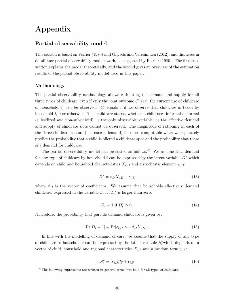
Appendix

Partial observability model

This section is based on Poirier (1980) and Ghysels and Vercammen (2012), and discusses indetail how partial observability models work, as suggested by Poirier (1980). The first sub-section explains the model theoretically, and the second gives an overview of the estimationresults of the partial observability model used in this paper.

Methodology

The partial observability methodology allows estimating the demand and supply for allthree types of childcare, even if only the joint outcome Ci (i.e. the current use of childcareof household i) can be observed. Ci equals 1 if we observe that childcare is taken byhousehold i, 0 or otherwise. This childcare status, whether a child uses informal or formal(subsidized and non-subsidized), is the only observable variable, as the effective demandand supply of childcare slots cannot be observed. The magnitude of rationing in each ofthe three childcare sectors (i.e. excess demand) becomes computable when we separatelypredict the probability that a child is offered a childcare spot and the probability that thereis a demand for childcare.

The partial observability model can be stated as follows.46 We assume that demandfor any type of childcare by household i can be expressed by the latent variable D∗i whichdepends on child and household characteristics Xi,D and a stochastic element εi,D:

D∗i = βDXi,D + εi,D (13)

where βD is the vector of coefficients. We assume that households effectively demandchildcare, expressed in the variable Di, if D∗i is larger than zero:

Di = 1 if D∗i > 0 . (14)

.Therefore, the probability that parents demand childcare is given by:

Pr[Di = 1] = Pr[εi,D > −βDXi,D] . (15)

In line with the modelling of demand of care, we assume that the supply of any typeof childcare to household i can be expressed by the latent variable S∗i which depends on avector of child, household and regional characteristics Xi,S and a random term εi,S :

S∗i = Xi,SβS + εi,S (16)46The following expressions are written in general terms but hold for all types of childcare.

35

where βS reflects the vector of coefficients. Similar to observed demand, we assume thateffective supply of a childcare slot to household i is observed is S∗i is larger than zero:

Si = 1 if S∗i > 0 . (17)

Consequently, the probability of being offered a childcare spot is given by:

Pr[Si = 1] = Pr[εi,S > −βSXi,S ] . (18)

In the data we only observe information on whether a household i uses care (Ci = 1)or does not (Ci = 0). However, this can be expressed as the joint outcome of both latentvariables demand D∗i and supply S∗i . The probability that someone is observed to usechildcare is given by the joint probability that this person demands care and the probabilitythat they are offered a childcare spot. In line with Poirier (1980), we assume that therandom terms of demand (Equation 13) and supply (Equation 16) are standard normallydistributed and cross-correlated through correlation parameter ρ as in a bivariate probitmodel. The probability of observation can be written as follows:

Pr[Ci = 1] = Pr[Si = 1 ∧Di = 1] (19)

Given Equations (13) to (18), the probability that we observe childcare usage can bewritten as follows:

Pr[Ci = 1] = Φ(βDXi,D, βSXi,S , ρ) (20)

where Φ denotes the bivariate standard normal distribution and ρ refers to the correlationbetween the random terms of the underlying demand and supply functions.

In addition, the probability that no childcare use is observed can also be written as ajoint outcome of demand and supply:

Pr[Ci = 0] = 1− Pr[Ci = 1]

= [1− Φ(βDXi,D, βSXi,S , ρ)] . (21)

Given Equations 20 and 21, the likelihood function L is equal to:

L(βD, βS , ρ) = Σni=1 Ci ln [Φ(βDXi,D, βSXi,S , ρ)] + (1− Ci) ln [1− Φ(βDXi,D, βSXi,S , ρ)]

(22)Once the coefficients of the covariates of the likelihood function are estimated, the

probabilities of being offered a spot in each childcare type can be derived. These estimates

36

are used in the labor supply model for the estimation of the model and the derivation ofthe budget constraints.

Estimation results

In the following tables we provide the results of the intermediary estimation of the demandand supply of childcare services in total and the three types of childcare services separatelythrough four partial observability probit procedures. We refer to the text for a discussion ofthe identifying variables that are specific to each equation. Table (12) highlights the resultsof the bivariate regression of demand for and access to (i.e. supply of) grandparental care.47

Table (14) presents the estimation results for demand and supply in the formal subsidizedchildcare sector, and Table (16) shows the estimation results for the non-subsidized childcaremarket. The final tables reflect the estimates of the procedure for total childcare servicedemand and supply.

47Note that demand and supply are estimated simultaneously but due to limits of space, we provide theresults in two separate tables.

37

Table 12: Bivariate regression of grandparental care

Demand for care by grandparents Coef. Std. Err.Age of the youngest child (in months) -0.322 ** 0.103Age² 0.008 ** 0.002Number of children 0.298 0.307Age of mother -0.023 0.041Child with special needs (parental assessment)(0/1) 0.154 0.944Marital status (reference = married couple)2. Single parent 2.632 ** 1.2353. Non-maritally cohabiting -0.011 0.395Maternal grandmother’s involvement in paid laborduring childhood of mother2. During part of childhood 0.638 0.5723. Not at all 0.840 ** 0.405Mother’s educational level (reference = up to primaryschool)3. Secondary school education -0.891 0.9064. Higher education -2.139 ** 0.892Mother’s preference regarding task division withpartner (reference = male breadwinner family)2. Mother with less time-demanding job than father -0.515 0.5643. Partners with equally demanding jobs -0.444 0.5594. Other -0.628 0.635Mother in fair health (self-assessed)(0/1) -0.189 0.352Father’s first preference regarding care isgrandparent (0/1)

1.781 ** 0.428

Father’s economic status (reference = father notpresent)1. Full-time job 0.168 0.4982. Part-time job 0.514 0.623Constant 4.167 ** 1.877The following page contains the second part of the estimates

38

Table 13: Bivariate regression of grandparental care (continued)

Supply of grandparental care Coef. Std. Err.Belongs to previous table

Age of the youngest child in months 0.162 ** 0.078Age² -0.004 ** 0.002Number of children in the household -0.335 * 0.187Mother’s age (years) -0.024 0.029Child with special needs (parental assessment) (0/1) 0.365 0.685Marital status (reference = married couple)2. Single parent -1.261 ** 0.5243. Non-maritally cohabiting -0.147 0.320Maternal grandmother’s involvement in paid laborduring childhood of mother (reference = over fullperiod)2. During part of childhood -0.570 0.4113. Not at all -0.975 ** 0.278Mother’s educational level (reference = up to primary)3. Secondary school education 0.139 0.3384. Higher education 1.045 ** 0.412Type of municipality (reference = residential)2. Rural community -0.079 0.2203. Economically concentrated or tourist -0.175 0.2304. Semi-urban -0.496 ** 0.2335. Urban -0.399 ** 0.200Childcare coverage in municipality (FTE/1000 0-2-yearolds)

0.669 0.688

Number of grandparents -0.056 0.075Grandparental availability index (health. workingstatus. living distance from family home)

0.242 ** 0.075

Constant -0.714 1.170N=869. selection: families with child(ren) below 3 of FFCS (2004-2005)

Likelihood-ratio test of rho=0 chi²(1)=0.514; use correctly predicted: 86%

Significance values * >90%. ** >95%. Log-likelihood = -285.549

39

Table 14: Bivariate regression of subsidized formal childcare

Demand for care by subsidized formal care Coef. Std. Err.Age of the youngest child in months 0.200 ** 0.042Age² -0.005 ** 0.001Number of children -0.156 ** 0.068Age of mother (years) -0.008 0.012Child with special needs (parental assessment)(0/1) -0.444 0.357Marital status (reference = married couple)2. Single parent 0.418 0.3543. Non-maritally cohabiting -0.025 0.136Maternal grandmother’s involvement in paid laborduring childhood of mother (reference = during fullperiod)2. During part of childhood -0.482 ** 0.1683. Not at all -0.472 ** 0.169Mother’s educational level (reference = up tot primary)3. Secondary school education 0.282 0.1964. Higher education 0.858 ** 0.240Household income is below the poverty line (0/1) 0.043 0.280Owner of own house (0/1) 0.291 0.181Taxable value of the house (euros) 0.000 0.000Mother’s preference of task division with partner(reference category: male breadwinner family)2. Mother with less time demanding job than father 0.589 ** 0.1883. Partners with equally demanding jobs 0.482 ** 0.1904. Other 0.389 0.251Mother in reasonable health (self assessed)(0/1) 0.000 0.188Formal care is father’s first choice (0/1) 1.062 ** 0.107Predicted supply of grandparental childcare -0.941 ** 0.429Father’s employment (reference = father not present)1. Full-time 0.092 0.2602. Part-time -0.520 0.401Constant -2.319 ** 0.609The following page contains the second part of the estimates

40

Table 15: Bivariate regression of subsidized formal childcare (continued)

Supply for care by subsidized formal care Coef. Std. Err.Belongs to previous tableAge of the youngest child in months -0.688 ** 0.219Age² 0.016 ** 0.005Number of children 0.575 ** 0.221Age of mother (years) 0.156 ** 0.042Child with special needs (parental assessment) (0/1) -0.993 * 0.571Marital status (reference = married couple)2. Single parent 4.181 ** 1.0593. Non-maritally cohabiting 0.900 ** 0.457Mother’s educational level (reference = up to primary)3. Secondary school education 0.337 0.6344. Higher education 0.053 0.634Household income is below the poverty line (0/1) -2.670 ** 0.647Type of municipality (reference = residential)2. Rural community -0.523 0.3823. Economically concentrated or tourist -1.388 ** 0.3684. Semi-urban 1.611 * 0.9615. Urban 0.838 0.563Childcare coverage in municipality (FTE/1000 0-2 yearolds)

-1.893 1.303

Proportion of formal care is non-subsidizedcenter-based care

-3.436 ** 1.182

Proportion of formal care is non-subsidized home-basedcare

1.144 1.407

Constant 3.056 2.387N=870. selection: families with child(ren) below 3 of FFCS (2004-2005)

Likelihood-ratio test of rho=0 chi²(1)=5.206**; use correctly predicted: 74%

Significance values * >90%. ** >95%. Log-likelihood = -451.885

41

Table 16: Bivariate regression of non-subsidized formal childcare

Demand for non-subsidized formal childcare Coeff. Std. Err.Age of the youngest child in months 0.024 0.052Age² -0.001 0.001Number of children -0.237 ** 0.081Age of mother (years) 0.047 ** 0.016Child with special needs (parental assessment) (0/1) -0.337 0.431Marital status (reference = married couple)2. Single parent 0.795 0.5853. Unmarried cohabition -0.094 0.153Educational level of mother (reference = up toprimary)3. Secondary school education 0.533 * 0.2954. Higher education 1.185 ** 0.322Family income is below the poverty line (0/1) 3.698 ** 1.841Home owner (0/1) -0.516 ** 0.203Taxable value of family house (euro) 0.000 ** 0.000Maternal grandmother’s involvement in paid laborduring childhood of mother (reference = during fullperiod)2. During part of childhood 0.113 0.1823. Not at all -0.035 0.189Mother’s preference of task division with partner(reference: male breadwinner family)2. Mother with less time-demanding job than father 0.263 0.2213. Partners with equally demanding jobs 0.367 * 0.2204. Other 0.293 0.277Father’s first choice of childcare service (reference =father not present)1. Formal care 0.180 0.1722. Informal care -0.524 ** 0.2303. Other -0.048 0.232Predicted supply of grandparental childcare -1.335 ** 0.481Predicted supply of subsidized formal childcare -0.889 ** 0.277Father’s employment (reference = father not present)1. Full-time 1.155 ** 0.4862. Part-time 1.112 ** 0.529Constant -2.679 ** 0.860The following page contains the second part of the estimates

42

Table 17: Bivariate regression of non-subsidized formal childcare (continued)

Supply of non-subsidized formal childcare Coef. Std. Err.Belongs to previous table

Mother’s age (years) -0.127 ** 0.039Marital status (reference = married couple)2. Single 1.131 ** 0.4723. Unmarried cohabition 2.406 ** 0.913Mother is in fair health (self assessed) (0/1) 0.334 0.579Mother’s educational level (reference = up to primary)3. Secondary school education 0.535 0.4784. Higher education 1.368 ** 0.411Family income is below poverty threshold (0/1) -2.683 ** 0.829Type of municipality (reference = residential)2. Rural community 1.378 ** 0.3993. Economically concentrated or tourist 0.455 0.2914. Semi-urban -1.436 ** 0.3635. Urban 0.154 0.244Childcare coverage in municipality (FTE/1000 0-2 yearolds)

4.760 ** 1.585

Proportion of formal care is non-subsidized childcarecentres

1.184 0.862

Proportion of formal care is non-subsidizedchildminders

1.042 0.820

Constant 1.281 1.404Significance levels: * >90%. **>95%; Use correctly predicted:

83%

Selection: Families with child(ren) below 3 of FFCS 2004-2005;

N = 870. Log likelihood = -347.885 ; Likelihood-ratio test of rho

= 0 chi²(1) = 2.779*

43

Table 18: Bivariate regression of childcare

Demand for any type of childcare Coeff Std. Err.Age of youngest child in months 0.205 ** 0.041Age² -0.006 ** 0.001Number of children -0.186 ** 0.068Age of mother (years) -0.045 ** 0.015Child with special needs (parental assessment) (0/1) -0.527 0.331Marital status (reference = married couple)2. Single parent 1.241 ** 0.3793. Non-maritally cohabiting -0.045 0.156Educational level of mother (reference = up toprimary)3. Secondary school education 0.755 ** 0.2044. Higher education 1.290 ** 0.190Mother’s preference of task division with partner(reference category: male breadwinner family)2. Mother with less time-demanding job than father 1.004 ** 0.1953. Partners with equally demanding jobs 0.936 ** 0.1884. Other 0.481 ** 0.241Maternal grandmother’s involvement in paid laborduring childhood of mother (reference = during fullperiod)2. During part of childhood -0.194 0.1723. Not at all 0.033 0.140Mother’s health (self-reported to be “fair”. 0/1) -0.033 0.164Household income is below the poverty line (0/1) -0.184 0.343Family is home owner (0/1) 0.021 0.223Taxable value of the house (euros) 0.000 ** 0.000Father’s employment status (reference: father notpresent)1. Working full-time 0.848 ** 0.2232. Working part-time 0.882 * 0.457Constant -1.503 ** 0.647Following page contains second part of estimates

44

Table 19: Bivariate regression of childcare (continued)

Supply of any type of childcare Coef. Std. Err.Belongs to previous table

Age of the youngest child (months) 0.063 0.042Age of the child squared (months squared) -0.002 ** 0.001Number of children -0.241 ** 0.079Mother’s age (years) 0.079 ** 0.019Child with special needs (parental assessment) (0/1) -0.107 0.349Marital status (reference = married couple)2. Single parent 0.461 0.4313. Unmarried cohabition 0.418 ** 0.191Maternal grandmother’s involvement in paid laborduring childhood of mother (reference = during fullperiod)2. During part of childhood -0.039 0.1833. Not at all -0.386 ** 0.140Mother’s educational level (reference = up to primary)3. Secondary school education -0.268 0.3914. Higher education 0.292 0.387Type of municipality (reference = residential)2. Rural community 0.194 0.1703. Economically concentrated or tourist -0.121 0.1614. Semi-urban -0.477 ** 0.1725. Urban 0.073 0.156Childcare coverage in municipality (FTE/1000 0-2 yearolds)

2.522 ** 0.771

Household income below the poverty line (0/1) -1.121 ** 0.287Number of grandparents living 0.243 ** 0.072Grandparental availability index (health. workingstatus. living distance from family home)

-0.108 ** 0.046

Constant -2.441 ** 0.916Significance levels: * >90%. **>95%; Use correctly predicted:

79%

Selection: Families with childr(en) below 3 of FFCS 2004-2005;

N = 870. Log likelihood = -405.554 ; Likelihood-ratio test of rho

= 0 chi²(1) = 24.624**

45

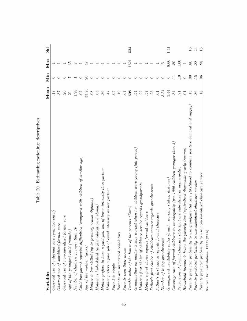
Tab

le20

:Estim

atingration

ing:

descriptives

Variables

Mean

Min

Max

Sd

Observeduseof

inform

alcare

(grand

parental)

.17

01

Observeduseof

subsidized

form

alcare

.37

01

Observeduseof

non-subsidized

form

alcare

.20

01

Age

oftheyoun

gest

child

(mon

ths)

217

35Num

berof

child

renyoun

gerthan

161.98

17

Child

hasparent-reporteddifficulties

(com

paredwithchild

renof

simila

rage)

.02

01

Age

ofthemother(years)

33.25

2047

Motheris

low-skilled(upto

prim

aryschool

diplom

a).08

01

Motheris

high-skilled(highereducationdiplom

a).63

01

Motherprefersto

have

apaid

job.

butof

lower

intensitythan

partner

.36

01

Motherprefersapaid

jobof

equa

lintensity

asherpartner

.47

01

Parentis

single

.05

01

Parents

areun

married

cohabitors

.19

01

Parents

owntheirhouse

.67

01

Taxable

valueof

thehouseof

theparents(E

uro)

608

01621

534

Grand

motheron

mother’sside

workedwhenherchild

renwereyoun

g(fullp

eriod)

.54

01

Mother’sfirst

choice

ofchild

care

serviceregardsgran

dparents

.22

01

Mother’sfirst

choice

regardsform

alchild

care

.57

01

Father’s

first

choice

ofchild

care

serviceregardsgran

dparents

.23

01

Father’s

first

choice

regardsform

alchild

care

.61

01

Num

berof

livinggran

dparents

3.54

06

Grand

parent

availabilityindex(health

.working

status.distan

ce)

3.44

08.66

1.41

Coveragerate

ofform

alchild

care

inmun

icipality(per

1000

child

renyoun

gerthan

3).34

.11

.80

Proportionof

form

alchild

care

slotsthat

aresubsidized

inmun

icipality

.71

.19

1.00

Hou

sehold

incomeis

belowthepovertylin

e(equivalized

disposable

yearly

income)

.01

01

Parents

predictedprobability

tousegran

dparentalc

are(likelihoodto

combine

positive

deman

dan

dsupply)

.15

.00

.80

.16

Parents

predictedprobability

tousesubsidized

child

care

service

.36

.15

.88

.24

Parents

predictedprobability

touseno

n-subsidized

child

care

service

.18

.06

.98

.15

Source:OwnCalculation

s.FFCS(2005)

46

Additional tables

• Descriptives of the sub-sample on which the model is estimated:

Table 21: Descriptive statistics sub-sample

CouplesMother Father

Average working time/week (hours) 27.44 42.01Average hourly gross wage 16.96 18.86Participation (%) 80.66 100Average age 33.25 36.78University degree (%) 62.70 49.22Presence of child 0-3 (%) 100Presence of child 4-6 (%) 37.70Presence of child 7-9 (%) 15.23Presence of child 10-12 (%) 9.18Presence of child 13-15 (%) 4.88Amount of observations 512Source: FFCS (2005). own calculations

• Wage regression in order to be able to derive gross labor income at each discrete laborsupply point:

Table 22: Hourly wage regression women

Dependent variable: ln hourly wage Coeff. Std. error

Age .00231 .032160Age squared .00011 .000486Civil servant .05576 .037624Experience .000034* .000796No degree -.37787* .158335Primary degree -.60236* .175674Low secondary degree -.49724* .056266High secondary degree -.23731* .031096Constant 2.65311* .519557*Significant on 5% level

Source: Own Calculations. FFCS (2005)

47

Copyright © 2013 @ the author(s). Discussion papers are in draft form. This discussion paper is distributed for purposes of comment and discussion only. It may not be reproduced without

permission of the copyright holder. Copies of working papers are available from the author.