Clemson UniversityTigerPrints

All Theses Theses

12-2017

Materials Properties of the Lepidopteran Proboscisand a Bio-Inspired Characterization Method ofCapillary AdhesionLuke Michael SandeClemson University

Follow this and additional works at: https://tigerprints.clemson.edu/all_theses

This Thesis is brought to you for free and open access by the Theses at TigerPrints. It has been accepted for inclusion in All Theses by an authorizedadministrator of TigerPrints. For more information, please contact kokeefe@clemson.edu.

Recommended CitationSande, Luke Michael, "Materials Properties of the Lepidopteran Proboscis and a Bio-Inspired Characterization Method of CapillaryAdhesion" (2017). All Theses. 2770.https://tigerprints.clemson.edu/all_theses/2770

MATERIALS PROPERTIES OF THE LEPIDOPTERAN PROBOSCIS AND A

BIO-INSPIRED CHARACTERIZATION METHOD OF CAPILLARY ADHESION

A Thesis

Presented to

the Graduate School of

Clemson University

In Partial Fulfillment

of the Requirements for the Degree

Master of Science

Materials Science and Engineering

by

Luke Michael Sande

December 2017

Accepted by:

Dr. Konstantin G. Kornev, Committee Chair

Dr. Olga Kuksenok

Dr. Peter Adler

ii

ABSTRACT

The feeding device of butterflies and moths, Lepidoptera, is called the “proboscis”

and it consists of two complex-shaped fibers, galeae, which get linked together when the

insects emerge from the pupa. The proboscis has been extensively studied by biologists,

but has never been investigated from the materials science point of view. The following

questions remain to be answered: What are the materials properties of the proboscis? How

does the proboscis assemble and repair and what role do capillary forces play? What are

the adhesion forces holding the galeae together during this assembly process?

We have investigated and are exhibiting a methodology for studying the self-

assembly and self-repair mechanism of the split lepidopteran proboscis in active and

sedated butterflies. The proposed method can be extended to a bio-inspired

characterization method of capillary adhesion for use with other samples. To probe the

repair capabilities, we have separated the proboscis far from the head with a metal post of

diameter comparable to the butterfly galea and moved the post ever closer to the head in

increments of 500 microns until the proboscis was fully split. Once split, we brought the

post back towards the tip in steps and observed the convergence of the two galeae back

into one united proboscis. To determine the materials properties of the proboscis, the

process of galeae gathering was filmed with a high speed camera. The galea profile,

extracted from each frame of the videos, was then fitted with a mathematical model based

on the Euler-Bernoulli beam theory where each galea was treated as a beam undergoing

small deflections. The theory was augmented by introducing the bending moments

modeling the muscular action and by a capillary force due to the saliva meniscus.

iii

Experiments on sedated butterflies, when the muscular action was diminished but saliva

was present, show the crucial role of the saliva meniscus in bringing galeae together. The

model sheds light on the evolutionary development of the butterfly proboscis.

iv

ACKNOWLEDGMENTS

We would like to acknowledge the National Science Foundation (NSF) for their

continued support on these works. This project was funded by NSF Projects: POL-

S1305338 and IOS-1354956.

This research was also supported in part by an appointment to the Student Research

Participation Program at the U.S. Air Force Civil Engineering Center (AFCEC)

administered by the Oak Ridge Institute for Science and Education (ORISE) through

interagency agreement between the U.S. Department of Energy and AFCEC.

Furthermore, I would like to acknowledge the following people: Dr. Kornev and

the Kornev group members, Pavel Aprelev and Chengqi Zhang, who have helped me every

step of the way during the course of my graduate school career; all of the Clemson

undergraduate students, Allison Kaczmarek, Alex Chernyk, and Madisen Weaver (a

Research Experiences for Undergrads (REU) summer student from Texas State University)

who assisted in data collection for my thesis; collaborators from the Department of Plant

& Environmental Sciences at Clemson University, Dr. Peter Adler, Dr. Charles (Eddie)

Beard, and Suellen Pometto; and the MS&E Director of Analytical Services, Kim Ivey, for

all of the help with dynamic mechanical analysis of the butterfly proboscises.

v

TABLE OF CONTENTS

Page

TITLE PAGE .................................................................................................................... i

ABSTRACT ..................................................................................................................... ii

ACKNOWLEDGMENTS .............................................................................................. iv

LIST OF TABLES ......................................................................................................... vii

LIST OF FIGURES ........................................................................................................ ix

CHAPTER

I. INTRODUCTION ......................................................................................... 1

1.1 Principles of Adhesion ....................................................................... 1

1.2 The Peel Test...................................................................................... 4

1.3 Introduction to Lepidoptera: The Butterfly

Proboscis ............................................................................................ 9

II. RESEARCH OBJECTIVE .......................................................................... 13

2.1 Motivation of Study ......................................................................... 13

2.2 Bio-Inspired Adhesion Characterization Method ............................ 13

III. RESEARCH METHODOLOGY................................................................. 17

3.1 Splitting of the Butterfly Proboscis.................................................. 17

3.2 Data Acquisition and Analysis......................................................... 42

IV. RESULTS AND DISCUSSION .................................................................. 51

4.1 Materials Properties of the Butterfly Proboscis ............................... 51

V. CONCLUSIONS.......................................................................................... 68

vi

Table of Contents (Continued)

Page

VI. SIGNIFICANCE OF WORK ...................................................................... 71

6.1 Reference Adhesion Experiment Using Ribbons

of Well Characterized Materials ...................................................... 71

APPENDICES ............................................................................................................... 79

A: Table of Collected Data ............................................................................... 80

B: Glossary of Parameters ................................................................................ 81

C: DMA Data .................................................................................................... 83

D: Wolfram Mathematica® Code ...................................................................... 84

E: Integration Constants for Solutions to Differential

Equations................................................................................................ 94

F: National Instruments LabVIEW® Code ....................................................... 96

REFERENCES ............................................................................................................ 105

vii

LIST OF TABLES

Table Page

1 Ranges of usable γ values when changing parameters B

and L, or the crack length, are shown by n1/n2 in

the table; any B-L pairs where waves always

propagate in our solution are unusable and are

shown by the red blocks in the table. This table can

be read as follows: for a certain B-L pair, we have

n1/n2 in the table and the n1, or number before the

backslash, is the first γ value that can be used for

this pair. Similarly, n2, or the number after the

backslash, is the largest value that can be used for

this pair. These γ=n1 and γ=n2 values were found

by plugging the designated B and L values into our

solution, setting the meniscus length, or length of

the wet region, equal to the length of the crack L,

and then searching through γ values until profiles

matching our physical case were be found. If the

profile dipped below the axis of symmetry (shown

by the dotted line in Figures 4 and 5) at any point,

then we couldn’t use that γ value. Additionally, if

waves start to propagate in our solution for a certain

γ, then we also cannot use this γ value. This table

was made for θ = π/2 and values are subject to

change for other θ values. The cells in green

display that for different B-L pairs corresponding to

different fiber shapes, lengths, and rigidities, ranges

of gamma values can remain similar. Therefore, in

our data fitting we have used γ=0.62 which seems

to fit the most fiber types. ...................................................................... 33

2 B values (data shown in Figure 17) collected for each

butterfly with their corresponding standard

deviations. The standard deviations were found by

considering each video and taking measurements of

B frame by frame. In this data set, 6 Monarchs and

5 Painted Ladies were tested to make up the 8 and

10 videos tested for each species, respectively. All

other collected data can be found in the appendices. ............................. 57

viii

List of Tables (Continued)

Table Page

3 The Modulus of Elasticity, E, values calculated from

equation [30] with average B values for each

butterfly species tested. The column indicated

‘Average’ is calculated with the Average B value

for each species whereas the ‘Low Estimate’ and

‘High Estimate’ are calculated with the upper and

lower B values that would be found based on our

standard deviation respectively. For further

clarification, higher B values lead to lower E values. ............................ 59

4 Comparison between the Modulus of Elasticity E

values found from the theoretical curve fitting and

the mechanical testing after calculating the moment

of inertia with parameter values for Rg1, Rg2, and h

found near the middle of the proboscis. Values for

these parameters can be found in Table 5. This

table shows that when using shape estimates for the

galeae near the middle of the proboscis instead of

the tip, we find much better agreement between our

theory and mechanical experiments in both the

averages and the lower and upper bounds (when

using one standard deviation to calculate them). ................................... 62

5 Tabulated parameters used in modulus of elasticity E

calculations where the symbol is shown in

parenthesis and the corresponding units are shown

in brackets. ............................................................................................. 63

6 Contact angle measurements on the surface of treated

tungsten wires. ....................................................................................... 78

ix

LIST OF FIGURES

Figure Page

1 Energy model of the peel test where P is the pulling

force at angle θ from the substrate. da is the length

that the film debonded from the surface, b is the

width of the film, and h is the thickness of the film. ............................... 6

2 Force model of the peel test where P is the pulling force

at angle θ from the substrate and Fadx and Fady are

the resisting forces in the x and y directions

respectively. Additionally, b and h are the width

and thickness of the film, respectively. .................................................... 8

3 a) Scanning Electron Microscope (SEM) image of the

butterfly proboscis in the coiled state, b) the cross

section, and c) the single galea curled up. These

images were taken from (43). d) A cross section of

a single galea where the white circular tube is the

trachea, and the semi-circular cut-out at the top is

one half of the food canal. e) Displays the

emergence from the pupa, or ‘eclosion’, and that the

two galeae are separated at this moment and come

together with a series of coiling-uncoiling motions

along with saliva pumping (courtesy of D.

Monaenkova). ........................................................................................ 11

x

List of Figures (Continued)

Figure Page

4 Experimental Schematic for the adhesion

characterization method. Two fibers are separated

by a wire where the beam is shown by the black

profile, the wire is shown by the brown circle, the

liquid meniscus is shown by the blue curved line,

and angles α1, α2, 𝜑, and θ are dependent upon the

slope of the profile at the point of contact with the

wire, point A. Additionally, Lcrack is the length of

the crack from x=0 to A’, lwet is the length of the

wet region from x=0 to the meniscus location, and

ldry is the length of the dry region or air-gap

between the meniscus and A’. Vadx and Vady are

the tangential, x, and normal, y, components of

adhesion force, respectively. Fn is the normal force

created at the post. The Y(X) is the beam profile

and dy/dx is the slope of the beam at the point A. ................................. 15

5 a) Idealized profiles of two fibers (black) separated by a

wire (brown) at one end but together at the other.

Three different loading scenarios on the beam ends:

b) θ = π/2, purely normal force Fnx acting on the

beam, c) θ < π/2, compression of the beam created

by inward horizontal component of the normal

force, Fnx, and d) θ > π/2, tension of the beam due

to the outward acting horizontal components of the

force, Fnx. .............................................................................................. 16

xi

List of Figures (Continued)

Figure Page

6 a) Schematic for butterfly galeae separation experiment

where the butterfly is shown in black and orange in

the top right, its proboscis is shown in black, is

extending to the left, and is separated by a wire

shown as a red circle between the black profiles.

Positions x=0, x=lwet, and x=Lcrack are the crack

location, meniscus location relative to the crack

location, and the position of contact between the

galea and the wire, respectively. The wet region is

displayed by zone 1 which has liquid and is shown

with details in the insert below the schematic of the

butterfly. The dry region is shown by zone 2 which

has no liquid and thus, only has the distributed

moment. b) Zoom in of zone 1 where the orange

arrows represent the capillary force that varies

linearly with respect to the deflection of the

proboscis away from the neutral axis (shown by the

equation for p(x)) and the green curled arrows

represent the distributed moment m in the beam

which accounts for muscular action. c) Free-body-

diagram of the cut region from b) (shown by the

dashed blue lines), where M and V signify the

internal moment and shear force, respectively. ..................................... 19

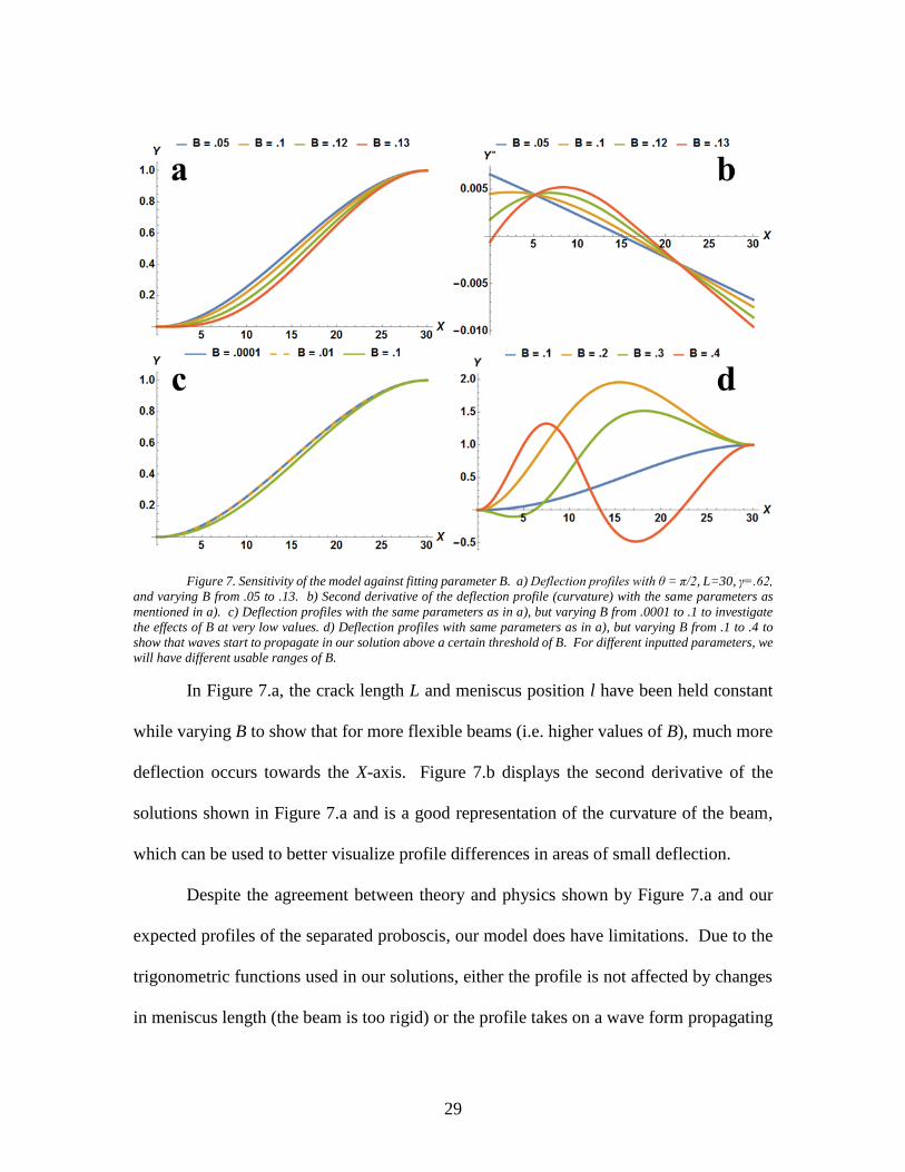
7 Sensitivity of the model against fitting parameter B. a)

Deflection profiles with θ = π/2, L=30, γ=.62, and

varying B from .05 to .13. b) Second derivative of

the deflection profile (curvature) with the same

parameters as mentioned in a). c) Deflection

profiles with the same parameters as in a), but

varying B from .0001 to .1 to investigate the effects

of B at very low values. d) Deflection profiles with

same parameters as in a), but varying B from .1 to

.4 to show that waves start to propagate in our

solution above a certain threshold of B. For

different inputted parameters, we will have different

usable ranges of B. ................................................................................. 29

xii

List of Figures (Continued)

Figure Page

8 Sensitivity of fittings to other parameters where L=30,

B =.13, and other parameters are varied. a) Varying

length of the wet region from l=0 to l=20 for γ=.62

and θ = π/2. b) Varying the angle θ from θ =23π/48

to θ =25π/48 for l=20 and γ=.62. c) While keeping

other parameters stable and l =15, varying the

dimensionless parameter γ from γ=.52 to γ=.77 by

changing the values of the post radius in the

parameter. For γ=.52, .62, and .77, post radii of

R=50 μm, 62.5 μm, and 75 μm were used,

respectively. ........................................................................................... 31

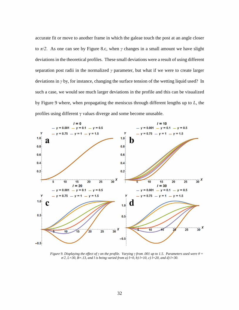
9 Displaying the effect of γ on the profile. Varying γ

from .001 up to 1.5. Parameters used were θ = π/2,

L=30, B=.13, and l is being varied from a) l=0, b)

l=10, c) l=20, and d) l=30. ..................................................................... 32

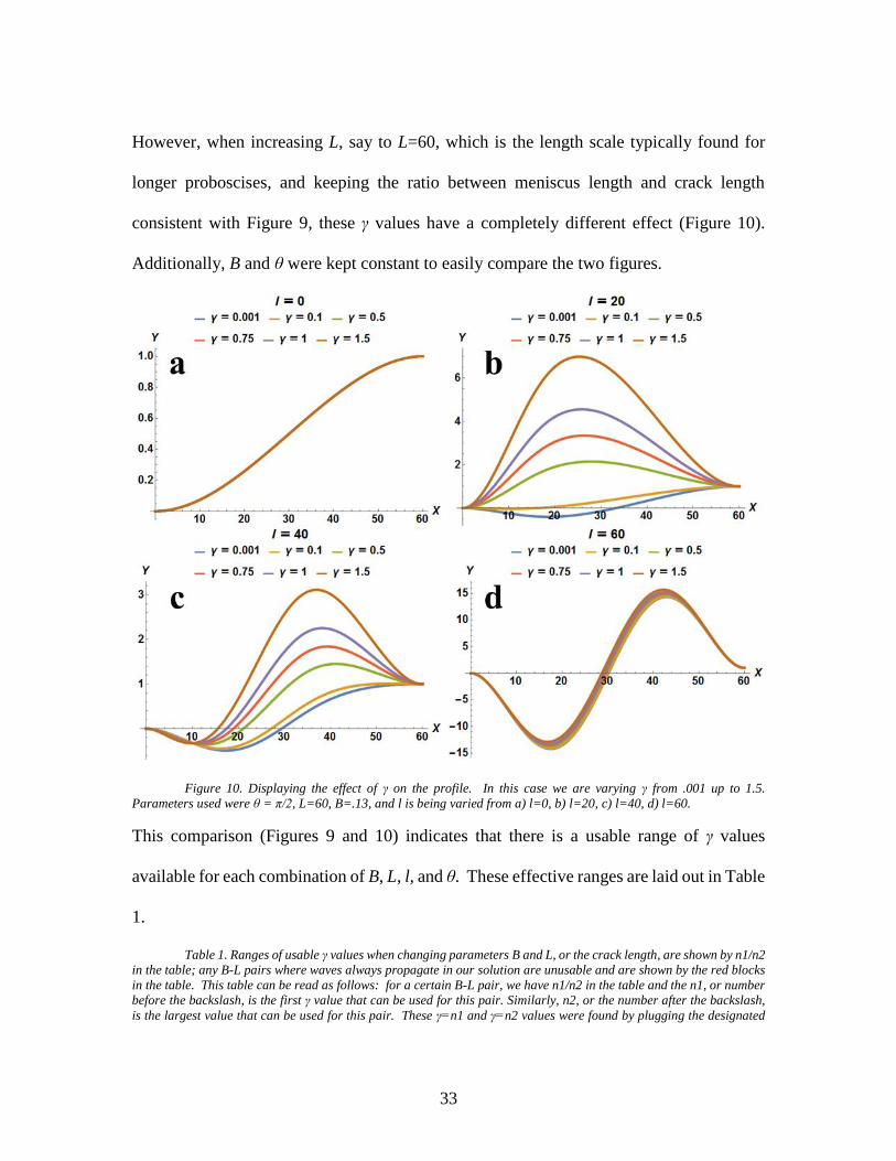
10 Displaying the effect of γ on the profile. In this case we

are varying γ from .001 up to 1.5. Parameters used

were θ = π/2, L=60, B=.13, and l is being varied

from a) l=0, b) l=20, c) l=40, d) l=60. ................................................... 33

xiii

List of Figures (Continued)

Figure Page

11 Experimental setup for proboscis separation and

butterfly sedation. a) Side view of the setup where

the butterfly is shown with its wings in paper

(shown by the transparent rectangle) and held

together with a clothespin (brown). The proboscis

(black line extending off of the head of the

butterfly) was extended and placed in a PDMS

clamp (not pictured) to ensure stability of the

galeae. The butterfly was sedated by using dry ice

in a warm water bath (beaker on a hot-plate shown

to right of the butterfly) to create a CO2 gas which

flowed out of the tube (green) via a showerhead

configuration to surround the butterfly with the gas.

After sedation the butterfly recovers completely

within a few minutes. b) Top view of the galea

separation experiment where the blue regions

between the galeae represent the saliva menisci and

the red signifies the separation post. c)

Experimental frames of the separated galeae

showing saliva propagation of a butterfly in the

“active” state, or before it has been dosed with

CO2. ....................................................................................................... 39

12 Flow-chart displaying data flow between LabVIEW

(green) and Mathematica (red) to outline the general

steps used in video/data analysis. The steps for

LabVIEW analysis can be found in this chapter, but

those used for data analysis in Mathematica can be

found in Chapter 3.2.3. .......................................................................... 44

13 a) Original, sample image of the butterfly proboscis

which had been split by a tungsten wire and b) the

binary (black and white) image with contours (thick

green lines) on the exterior of the proboscis and the

regions of interest shown by the thin green

rectangles situated at an angle parallel to the length

of the proboscis. ..................................................................................... 45

xiv

List of Figures (Continued)

Figure Page

14 Displaying the escape of saliva from the tip of the

proboscis and its propagation inside of the PDMS

clamp over time. The video was recorded at 30

FPS. ........................................................................................................ 52

15 Displaying the increasing of the meniscus retraction

length (LR) (normalized by the diameter of the post)

over time (t) and where the LR is measured by the

change in distance between the meniscus front and

the center of the post for butterflies in the sedation

process. The data (hollow circle points) were fit

with square-root-of-time kinetics as can be seen by

the solid colored lines. In this graph, each color is

representative of a single butterfly in a single video

and the data points were taken at each frame in the

videos where saliva retraction was seen. ............................................... 53

16 Butterflies undergoing sedation process: a) M213

141820 Sedating BG Frame 123, b) M213 141820

Sedating TG Frame 142. Video 2: c) M213 141820

Sedating BG Frame 124. Active butterflies: d) M12

120131 Awake BG Frame 0, e) M12 120131

Awake TG Frame 14, and f) M18 170354 Awake

BG Frame 301. ....................................................................................... 55

17 Displaying the average B values for Monarchs (shown

in orange and M on the legend) and Painted Ladies

(shown in purple and PL on the legend) in the active

state (A on legend), sedating state (Se), and sleeping

(anesthetized) state (Sl). It can be seen by the error

bars overlaying the data bars that for the case of

active butterflies, there is much more variability

than there is for sedated butterflies. Also, it is

worth noting that TG and BG signify Top Galea and

Bottom Galea, respectively. ................................................................... 56

xv

List of Figures (Continued)

Figure Page

18 Modulus of Elasticity values taken from DMA tensile

testing. This bar graph follows previous

conventions; orange represents monarchs tested,

purple represents the painted ladies tested, and the

green represents the average modulus of all

butterflies tested with an error bar showing one

standard deviation above and below the average.

The legend can be read as such; M stands for

Monarch and PL stands for Painted Lady, the

number afterwards represents the number of

butterflies tested, and A or B signifies the galea that

was tested from that butterfly. ............................................................... 61

19 Displaying the Capillary force (Fc) against the length of

the wet region along the length of the galeae. As

capillary length increases, we have a corresponding

increase in magnitude of capillary force and, thus, a

greater restoring force. In this figure, the orange

and purple dots represent data from Monarchs and

Painted Ladies, respectively. Additionally, the error

bars in the x and y directions are showing one

standard deviation for each of the data points. The

larger error bars correspond to tests on active

butterflies while those with smaller error bars are

typically sedated or sleeping butterflies. The linear

trendlines were added to guide the eye as to how the

data was acting. This raw data can be found in

supplemental information. ..................................................................... 65

20 Adhesion forces plotted against θ in the a) Horizontal

direction (Vadx) and b) Vertical direction (Vady).

In these figures, orange and purple dots correspond

to tests with Monarchs and Painted Ladies,

respectively. Error bars use the same conventions

as in previous figures. ............................................................................ 66

xvi

List of Figures (Continued)

Figure Page

21 Experimental setup for the reference experiment. a)

Side view of the experiment showing the wooden

clothespins, the syringe holder, syringe, and 90˚

angled needle used to send water between the

ribbons, the 500 μm separation tungsten wire

(shown by the vertical wire in the middle), the

tungsten ribbons (shown by the horizontal metallic

strip), and the tape holding them together at the

ends. b) Top view of the experiment showing the

top edge of the ribbons which have been separated

by the wire (500 μm). ............................................................................. 73

22 Typical contact angle measurement on the tungsten

ribbon. This particular image was taken of a ribbon

surface treated with trimethylethoxysilane and had a

contact angle of 49.5˚. ............................................................................ 77

1

CHAPTER ONE

INTRODUCTION

1.1 Principles of Adhesion

Adhesion can be defined as the tendency for two objects to be attracted to one

another when brought into close contact with each other (1, 2). This is true on the nano-

scale where atoms and molecules form quite strong bonds, but there is a paradox in that

statement because it is not always true on the macro, or engineering, scale. For instance,

if one placed two ceramic blocks together they would not simply stick together; one would

have to place an ‘adhesive’ such as glue, epoxy, or cement in between them to enhance the

interfacial attraction. Conversely, the molecules and atoms making up these ceramic

blocks adhere very well to each other, otherwise they would not form the large components

that they are comprising (1). Thus, the concept of adhesion is not well understood as of

yet.

The task of theoretically describing the work of adhesion between two objects, a

property which is ideally a characteristic of the joint and independent geometric parameters

of specimens, has been a significant challenge and thus, it is instructive to turn to the

simplest scenario of adhesion characterization, the peel test (Figure 1). Initially, scientists

attempted to analyze the peel test by considering the stress distribution around the peel

front but were met with little success due to the complex stress distributions around the

peel front (3-5). Others have attempted to use a fracture-mechanics method that considers

a stress intensity factor based upon a stress-singularity argument; however, this did not

prove successful either (3, 6, 7). Therefore, most people have adopted a simpler approach

2

that is not based on the complex stress distribution around the peel front or the

determination of the stress-intensity factor, and we will do the same (discussed in Chapter

1.2.1).

1.1.1 Benefits of Higher Adhesion at Fiber-Matrix Interface

In the past few decades, the use of fibers as reinforcements in matrices, including

polymers and ceramics, to create multifunctional materials has greatly increased due to the

capacity for such fibers to enhance the structural (strength, energy absorption, damping,

and fracture toughness among others) as well as non-structural properties of a material

(thermal conductivity, electromagnetic shielding, and energy storage for example) (8).

Since these fibers are now used for such a wide range of applications in multifunctional

materials, it is imperative to understand the role that the fiber-matrix interface plays on

such properties.

The interface between fibers and their surrounding matrix is a critical region that

determines many of the desired mechanical properties of a composite material, for it is

responsible for the load transfer from the matrix to the fibers and, hence, the quality of the

reinforcement itself (9, 10). At this interface, an interaction between two dissimilar

materials, depending on the chemical structure of both phases as well as their chemical

affinities for one another, will greatly affect measured adhesion energies. By surface

treating the reinforcing fibers, one can adjust the level of interactions at the interface to

increase or decrease the adhesion energy accordingly. Hoecker demonstrated this in 1995

by using various surface treatments on carbon-fibers in carbon-fiber-reinforced epoxy

3

resins and performing transverse and shear tests on the samples; with an improvement in

adhesion came an increase in mechanical properties (11). Likewise, the failure mode

changed from interfacial failure between the fibers and matrix to one of matrix failure when

adhesion was increased. Another study from 2011 performed by Lopez-Buendia added to

this correlation, with polypropylene (PP) fibers embedded in concrete (12). In addition to

an increase in mechanical properties, an enhanced fiber-matrix interface also leads to

increased energy dissipation, damping, and impact absorption as found by multiple

researchers in the past couple of decades (13-21). As discussed above, the strength of the

fiber-matrix interface in composites is an important aspect of the reinforcement and, thus,

a reliable and reproducible means for testing this interface, especially when performed in

different laboratories, is required to advance the state of the art.

The interface between a fiber and its surrounding matrix is critical in the transfer of

stress of the composite material (22); hence, it is important to have a reliable, repeatable,

and versatile characterization method that can be easily adapted to many different types of

samples.

1.1.2 Recent Advances in the Field of Adhesion

Of late, researchers have made many developments on the adjustment or

enhancement of the common adhesion tests such as the peel test and pull-out test among

others. For instance, Hassoune-Rhabbour has adjusted the pull-out technique by changing

the shape of the matrix so that it necks towards the fiber at the point of embedment on one

end and is perpendicular to the insertion of the fiber on the other end; this was intended to

4

lead to controlled, localized crack development at the flat end where the stress

concentration is higher (23). Moreover, Ostrowicki and Sitaraman created an interesting

variant of the peel test called the Magnetically Actuated Peel Test (MAPT) in which they

applied a permanent magnet to a specimen, placed it above an electromagnet a known

distance, and then ran a current through the electromagnet to create a controlled repulsive

force that imposes a peeling of the films from the substrate at a critical load; afterwards,

the delamination lengths of the films were measured and correlated with adhesion (24).

Additionally, there have been efforts to use vibrations and the inherent vibration damping

as a means for measuring the fiber-matrix adhesion of fiber reinforced composites (19, 25,

26). A method proposed by Narkis in 1988 relied on bending jigs to create curvature

changes in the fiber for adhesion characterization purposes; this was done to create a

desirable method that doesn’t depend on the longitudinal fiber strength or embedment

length to successfully perform experiments unlike other commonly used testing methods,

but it required further theoretical and experimental optimization before it could actually be

put to use (27). Only a brief review of the recent advances in the field of adhesion has been

mentioned above but, most of these are slight adjustments to existing methods and, thus,

are not groundbreaking new characterization methods viable for many applications.

1.2 The Peel Test

The most common testing method used for the measurement of adhesion between

thin films and a rigid substrate is the peel test; it has been used for adhesion characterization

applications ranging from solar cells (28) to polymer dielectrics (29) and is applicable for

5

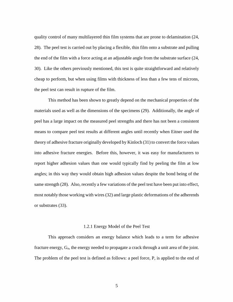
quality control of many multilayered thin film systems that are prone to delamination (24,

28). The peel test is carried out by placing a flexible, thin film onto a substrate and pulling

the end of the film with a force acting at an adjustable angle from the substrate surface (24,

30). Like the others previously mentioned, this test is quite straightforward and relatively

cheap to perform, but when using films with thickness of less than a few tens of microns,

the peel test can result in rupture of the film.

This method has been shown to greatly depend on the mechanical properties of the

materials used as well as the dimensions of the specimens (29). Additionally, the angle of

peel has a large impact on the measured peel strengths and there has not been a consistent

means to compare peel test results at different angles until recently when Eitner used the

theory of adhesive fracture originally developed by Kinloch (31) to convert the force values

into adhesive fracture energies. Before this, however, it was easy for manufacturers to

report higher adhesion values than one would typically find by peeling the film at low

angles; in this way they would obtain high adhesion values despite the bond being of the

same strength (28). Also, recently a few variations of the peel test have been put into effect,

most notably those working with wires (32) and large plastic deformations of the adherends

or substrates (33).

1.2.1 Energy Model of the Peel Test

This approach considers an energy balance which leads to a term for adhesive

fracture energy, Ga, the energy needed to propagate a crack through a unit area of the joint.

The problem of the peel test is defined as follows: a peel force, P, is applied to the end of

6

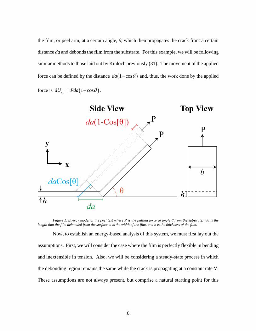
the film, or peel arm, at a certain angle, θ, which then propagates the crack front a certain

distance da and debonds the film from the substrate. For this example, we will be following

similar methods to those laid out by Kinloch previously (31). The movement of the applied

force can be defined by the distance 1 cosda and, thus, the work done by the applied

force is 1 cosextdU Pda .

Figure 1. Energy model of the peel test where P is the pulling force at angle θ from the substrate. da is the

length that the film debonded from the surface, b is the width of the film, and h is the thickness of the film.

Now, to establish an energy-based analysis of this system, we must first lay out the

assumptions. First, we will consider the case where the film is perfectly flexible in bending

and inextensible in tension. Also, we will be considering a steady-state process in which

the debonding region remains the same while the crack is propagating at a constant rate V.

These assumptions are not always present, but comprise a natural starting point for this

7

particular fracture mechanics problem. Now the energy analysis of this problem can be

initiated and written in terms of the energy release rate, G, where the adhesive fracture

energy density, Ga, can be found through [1]:

a a extG dA G bda dU

dA bda

[1]

Where dA is the increment of area created (b is the width of the film). Henceforth, for the

simple case that is infinitely rigid in axial tension (given a superscript of E ), we have an

adhesive energy of fracture per unit area shown by equation [2] below.

(1 cos )

1 cosE

a

Pda PG

bda b

[2]

This methodology can be extended to more complex cases such as one in which

tensile deformation of the peeling arm occurs due to the tensile stress (3); however, we will

not be using these results in these works and thus will not be going into further detail.

1.2.2 Force Model of the Peel Test

Now instead of an energy approach that was taken in the previous section, we will

be considering a quasi-static force balance for the peel test. When using a modified setup

as found by Figure 2, we can see that for the peel test a peeling force, P, is applied to one

end of the film while the other end is adhered to a substrate and the resisting forces, Fadx

and Fady, act in the x and y directions, respectively.

8

Figure 2. Force model of the peel test where P is the pulling force at angle θ from the substrate and Fadx and

Fady are the resisting forces in the x and y directions respectively. Additionally, b and h are the width and thickness of

the film, respectively.

When pulling on this film, one has to overcome a certain force threshold before the

film detaches from the surface of the substrate in any direction, but this force is not acting

completely in one direction; it has components in both the normal and tangential directions

due to the angle θ. Therefore, we can say that there is an adhesion force acting at the crack

location that holds the film to the substrate and resists the peeling force P in both the y,

normal, and x, tangential, directions relative to the substrate when assuming the substrate

surface extends in the x-direction. First, we will look at the force balance in the x-direction:

0 :

cos 0

cos

x

adx

adx

F

P F

F P

[3]

9

Where Pcos(θ) is the x-component of the peeling force P and Fadx is the force due to

adhesion acting in the x, or tangential, direction. Likewise, we can introduce the force

balance in the y-direction, where Fady is the force due to adhesion acting in the y-direction

and Psin(θ) is the y-component of the peeling force:

0 :

sin 0

sin

y

ady

ady

F

P F

F P

[4]

For the static case before the crack starts to propagate through the system, we can establish

the x and y components of the adhesion force by simply considering the force balance.

This simple method is advantageous over the energy approach due to the fact that

energy only considers the vertical bond between the film and the substrate while this

method also considers the horizontal; however, to extend it to dynamic systems where

movement of the crack is present, one would have to add the acceleration term in

Newtonian mechanics in place of the zero on the right hand side of the force balance and

this would be another unknown that would have to be measured experimentally.

1.3 Introduction to Lepidoptera: The Butterfly Proboscis

The mouthparts of lepidopterans, the order of insects composed of moths and

butterflies (34), are complex feeding apparatuses that make use of unique material

properties to keep the organs clean while the organism is drinking sticky and viscous

liquids. Specifically, the dichotomy of the wetting properties (35) along the length of the

lepidopteran proboscis, an interesting bio-fiber composed of two separate, semi-elliptical

10

organs known as galeae (Figure 3), is thought to assist in this process. The external surface

of the proboscis has a drinking region near the tip with hydrophilic properties and a non-

drinking region for the rest of the length (35). These wetting properties, combined with its

elliptical shape (Figure 3.b), help to create a larger meniscus in the hydrophilic region

which facilitates the entrance of the liquid into the food canal along with the feeding from

various types of sustenance ranging from floral nectar and sap to blood and dung (36). All

of the while, the butterfly proboscis remains clean from debris that could impede fluid

uptake due to the hydrophobic nature of the majority of the external surface (37-39).

However, the feeding functionality of the proboscis is not the only interesting mechanism

in the proboscis; the coiling and uncoiling capabilities for storage, usage, and assembly

(38, 40, 41), is a biomechanical feature that helps to create an intricate organ with many

possible bio-medical and mimetic applications in drug delivery and micro-fluidics (37, 42).

Before engineers will be able to replicate the fascinating capabilities of the butterfly

proboscis, however, the materials properties and assembly mechanism must be

investigated, quantified, and understood and thus, that is one particular goal of this work.

11

Figure 3. a) Scanning Electron Microscope (SEM) image of the butterfly proboscis in the coiled state, b) the

cross section, and c) the single galea curled up. These images were taken from (43). d) A cross section of a single

galea where the white circular tube is the trachea, and the semi-circular cut-out at the top is one half of the food canal.

e) Displays the emergence from the pupa, or ‘eclosion’, and that the two galeae are separated at this moment and come

together with a series of coiling-uncoiling motions along with saliva pumping (courtesy of D. Monaenkova).

In the past, the lepidopteran proboscis was thought to assemble only once during

the insect’s lifetime (40). This initial linking is facilitated via a series of coiling and

uncoiling motions immediately after eclosion (shown in Figure 3.e) during which the

cuticular structures known as the dorsal (top) and ventral (bottom) legulae interlock (38,

40); however, throughout this process, saliva is omnipresent which leads one to come to a

realization that saliva may actually play a significant role in the assembly of the

split/damaged proboscis. Recently, it was discovered that if the butterfly mouthparts are

separated, the butterfly can actually bring the galeae back together and repair the proboscis

12

back into one fiber (44). We hypothesize that by using a combination of muscular action

in the galeae, internal pressure from the hemolymph canals running through the galeae, and

capillary forces from liquid saliva which is being pumped from the head into the split

proboscis region, the butterfly can successfully bring the split galea back together into one

component. Our goal is to determine the role that saliva plays in the repair of the proboscis

and estimate the longitudinal Young’s Modulus of Elasticity (E) of the single galea as well

as the adhesion force between the galeae for use in bio-mimetic and micro-fluidic

transportation devices (37, 42) further down the road.

13

CHAPTER TWO

RESEARCH OBJECTIVE

2.1 Motivation of Study

The proboscis has been well described by biologists in regard to its shape and

behavior across many species of Lepidoptera (34, 45). However, the proboscis has never

been studied from the materials science point of view and thus, there are many unknowns

that lead to questions such as: What are the role of capillary forces in proboscis assembly

or repair? What is the Modulus of Elasticity (E) of the proboscis? What are the adhesion

forces holding the galeae together in this repair process? Therefore, the goals of this study

are to find solutions to these problems by using the separated galeae profiles along with

Euler-Bernoulli beam theory. Additionally, due to the lack of repeatable adhesion

characterization techniques currently available, it is our goal to create an adhesion

characterization method founded on the deflection of fibers and useable with fiber-fiber

interactions or fiber-matrix adhesion cases.

2.2 Bio-Inspired Adhesion Characterization Method

After its emergence from the pupa or in the case of separation later in life, the

butterfly tries to unite the two galeae with a series of coiling-uncoiling motions along with

saliva pumping as shown by Figure 3.e. In this series of events, a saliva meniscus can be

seen propagating between the two fibers and it is hypothesized that this saliva column helps

to bring the galeae together with capillary and adhesion forces. This idea is supported by

recent findings that show that capillary forces are strong enough to bend and greatly deform

14

slender structures, such as fibers and wires (46-49). The butterfly proboscis is modeled by

this scenario due to its high aspect ratio (long and thin) and the saliva propagation in the

assembly/repair process. Henceforth, we have studied the self-repair mechanism by

separating the galeae, straightening the fibers, keeping them separated with a wire far away

from its head, and then observing any repair that occurred. The similarities in geometry

between this galeae separation experiment and the peel test sparked the idea to create a

new experiment founded on the concepts of fiber separation and adhesion.

Therefore, we have created a novel adhesion characterization method inspired by

this repair of the split Lepidopteran proboscis (Figure 4) and related to the force balance

that was displayed for the peel test in Figure 2. The experiment is comprised of two fibers

that are separated far away from their point of contact with each other by a wire of known

diameter, as depicted by the schematic in Figure 4. Hence, the fiber deflection relative to

the x-axis (black horizontal line in Figure 4) is known at the point of incidence A’. In the

previous peel test case, the force P and angle at which the film was being pulled, θ, were

known parameters; however, in our case, the normal force created by the contact between

the post and the fiber is not known and must be quantified to determine the unknown

adhesion forces at the point of fiber contact, x=0. To classify these forces, we have

implemented the Euler-Bernoulli beam theory (50) which is a simplification of the Euler-

Elastica theory (51) for the case of small deflections of the beam relative to its length. This

beam theory uses the profile and deflection of the fibers to calculate the shear forces in the

fibers or ‘beams’ and thus, allows us to calculate the normal force created at the post

position along with the interfacial adhesion forces between the two fibers in both the

15

normal and tangential directions. Further details as to how this problem was solved can be

found in Chapter 3.1.2.

Figure 4. Experimental Schematic for the adhesion characterization method. Two fibers are separated by a

wire where the beam is shown by the black profile, the wire is shown by the brown circle, the liquid meniscus is shown

by the blue curved line, and angles α1, α2, 𝜑, and θ are dependent upon the slope of the profile at the point of contact

with the wire, point A. Additionally, Lcrack is the length of the crack from x=0 to A’, lwet is the length of the wet region

from x=0 to the meniscus location, and ldry is the length of the dry region or air-gap between the meniscus and A’. Vadx

and Vady are the tangential, x, and normal, y, components of adhesion force, respectively. Fn is the normal force created

at the post. The Y(X) is the beam profile and dy/dx is the slope of the beam at the point A.

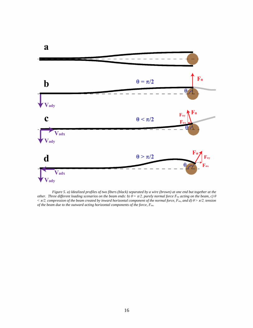
For this problem, we have three different cases of profile shape that could occur

due to the stiffness of the beams and the wire position and as such, we could have three

different loading scenarios: purely vertical forces, axial compression, and axial tension.

These scenarios are demonstrated by Figure 5 where Vadx, Vady, Fnx, Fny, and Fc are the x

and y components of adhesion force, the x and y components of the normal force Fn at the

position A’ (Figure 5), and the capillary force, respectively. Additionally, is the angle

between the x-axis and the vector A (Figures 4 and 5).

16

Figure 5. a) Idealized profiles of two fibers (black) separated by a wire (brown) at one end but together at the

other. Three different loading scenarios on the beam ends: b) θ = π/2, purely normal force Fnx acting on the beam, c) θ

< π/2, compression of the beam created by inward horizontal component of the normal force, Fnx, and d) θ > π/2, tension

of the beam due to the outward acting horizontal components of the force, Fnx.

17

CHAPTER THREE

RESEARCH METHODOLOGY

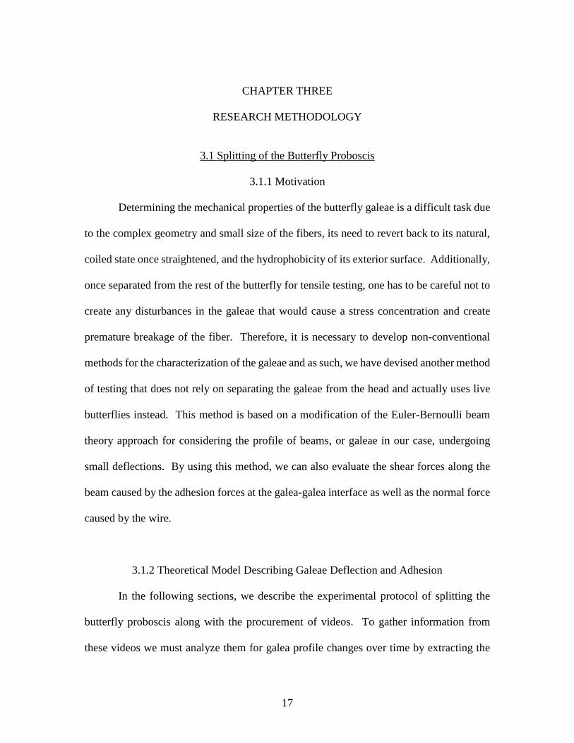
3.1 Splitting of the Butterfly Proboscis

3.1.1 Motivation

Determining the mechanical properties of the butterfly galeae is a difficult task due

to the complex geometry and small size of the fibers, its need to revert back to its natural,

coiled state once straightened, and the hydrophobicity of its exterior surface. Additionally,

once separated from the rest of the butterfly for tensile testing, one has to be careful not to

create any disturbances in the galeae that would cause a stress concentration and create

premature breakage of the fiber. Therefore, it is necessary to develop non-conventional

methods for the characterization of the galeae and as such, we have devised another method

of testing that does not rely on separating the galeae from the head and actually uses live

butterflies instead. This method is based on a modification of the Euler-Bernoulli beam

theory approach for considering the profile of beams, or galeae in our case, undergoing

small deflections. By using this method, we can also evaluate the shear forces along the

beam caused by the adhesion forces at the galea-galea interface as well as the normal force

caused by the wire.

3.1.2 Theoretical Model Describing Galeae Deflection and Adhesion

In the following sections, we describe the experimental protocol of splitting the

butterfly proboscis along with the procurement of videos. To gather information from

these videos we must analyze them for galea profile changes over time by extracting the

18

contour lines of the dark border separating the outer walls of the galeae from background

in the images. This video analysis algorithm will be further described in Chapter 3.2;

however, at this time it is important to introduce the mathematical model underlying the

contour fitting of the deflected galeae for the extraction of materials properties.

To characterize the materials properties of the butterfly proboscis, we have chosen

to use an augmented version of the well-understood Euler-Bernoulli beam theory, which is

used primarily to determine the load-bearing and deflection characteristics of beams when

subjected to lateral loads and small deflections (50). The reasoning behind the use of this

theory will become evident after establishing the force and moment balances acting on a

galea during the repair process. The galea profile is described by function y=y(x), Figure

6.

When splitting the proboscis of the butterfly and keeping them separated at a

distance far from the head, a liquid column of saliva can be seen propagating through the

food canal during which muscular contractions and expansions inside of the galeae work

to bring the galeae back together and eventually lock the legulae in place. The forces from

the muscular movements are being approximated by a distributed moment m of uniform

amplitude acting along the entire length of each galeae and the capillary force is being

modeled by [5] where 1F and 2F are constants. However, the capillary force is only acting

up to the saliva meniscus, and thus, we have two distinct zones to consider.

1 2( ) ( )p x F F y x [5]

19

Figure 6. a) Schematic for butterfly galeae separation experiment where the butterfly is shown in black and

orange in the top right, its proboscis is shown in black, is extending to the left, and is separated by a wire shown as a red

circle between the black profiles. Positions x=0, x=lwet, and x=Lcrack are the crack location, meniscus location relative

to the crack location, and the position of contact between the galea and the wire, respectively. The wet region is displayed

by zone 1 which has liquid and is shown with details in the insert below the schematic of the butterfly. The dry region is

shown by zone 2 which has no liquid and thus, only has the distributed moment. b) Zoom in of zone 1 where the orange

arrows represent the capillary force that varies linearly with respect to the deflection of the proboscis away from the

neutral axis (shown by the equation for p(x)) and the green curled arrows represent the distributed moment m in the

beam which accounts for muscular action. c) Free-body-diagram of the cut region from b) (shown by the dashed blue

lines), where M and V signify the internal moment and shear force, respectively.

3.1.2.1 Zone 1: Meniscus Region

For this zone, we have to incorporate all of the forces due to capillary action since

the liquid column is present here; thus, we will be taking into account the surface tension

as well as the capillary pressure inside of the liquid column approximated by [5]. Hence,

after making two cuts in the galea to expose internal forces (Figure 6) on each side of a

segment dx in length, the vertical force balance is as follows:

20

0 ( ) 0y

F V p x dx V dV . [6]

After simplifying [6], we are left with an expression for the change in internal shear force,

denoted by V :

dV

p xdx

. [7]

Similarly, we can sum moments on the galea to get an equilibrium expression with the

leftmost side of the cut portion with two exposed sides shown in Figure 6 with counter-

clockwise as our positive sign convention. This summation is shown in

2( )

0 02

p x dxM mdx M dM V dV dx . [8]

Simplifying [8] and neglecting higher order terms yields an expression for the change in

internal moment denoted by M :

dM

m Vdx

. [9]

Since we know that the internal shear force V changes along the x-direction, we can take

the first derivative of [9] which leads:

2

2( )

d M dmp x

dx dx [10]

Remembering the expression for the well-known Euler-Bernoulli relation:

''EIy x , [11]

where E is the longitudinal Young’s elastic modulus (a material property) and I is the area

moment of inertia (structural property) which is dependent on the cross sectional shape

21

(52). Taking the second derivative of [11] with respect to x gives an expression into which

we can input [5] and [10]. Thus, we arrive at our fourth order differential equation

1

1 1 2

'''' ( )

'''' ( )

dmEIy x p x

dx

EIy x F F y x

. [12]

In [12], we can neglect dm/dx by assuming that the butterfly is sedated; in this case, m is a

constant amplitude along the length of the galea and, thus, the 1st derivative of m with

respect to x would go to zero.

3.1.2.2 Zone 2: Air Gap

Similarly, we can set up the model for zone 2 where the liquid column has not

reached yet; thus, there are no capillary forces present, i.e. p(x)=0 and we only have to

consider the distributed moment m along the galea. As discussed directly above, this

distributed moment is of constant amplitude and therefore, the first derivative goes to zero

in this zone as well. Hence, we are left with the characteristic equation for zone 2:

2 '''' 0EIy x . [13]

3.1.2.3 Normalizing Differential Equations

Since both of these characteristic equations, [12] and [13], are fourth order

differential equations, we will need a series of boundary and continuity conditions,

specifically 8, to solve them together and create a fitting model from them. Before

establishing the boundary conditions, however, it is convenient to normalize equations [12]

and [13] by the radius of the post R; thus, we have y YR and x XR where Y and X

22

are dimensionless parameters for deflection and horizontal position along the length of the

proboscis respectively. The normalized equations can now rewritten as:

Zone 1: 3 4

1 21 1''''

F R F RY X Y X

EI EI [14]

Zone 2: 2 '''' 0Y X . [15]

Also, the ratios 4

2F REI

and 3

1F REI

are both dimensionless parameters. Note that the

dm/dx has been dropped prior to normalization due to reasons discussed previously.

3.1.2.4 Boundary Conditions

The angle θ, an important parameter which helps to define the shape of our beams

near the post, has been introduced in Figures 4 and 5. The boundary conditions are

specified as

1 1

2 2

0 0 ' 0 0

sin ' cot

0 ' 0

'' 0 ''' 0

Y Y

Y L Y L

Y l Y l

Y l Y l

[16]

where crackLL

R and wetl

lR

. In this equation set, 2Y L & 2 'Y L define the

deflection and slope of the beam at point A (Figure 4) and 1 2'' ''( ) ''( ) 0Y l Y l Y l is

a continuity condition that signifies that the second derivative of the deflection equations

in zones 1 and 2 must be equal at position l . Additionally, the zeroth, first, second, and

third derivatives of Y(X) correspond to the deflection, slope, moment, and shear force

distributions in the beam, respectively. The same conventions apply to the rest of the

23

conditions in equation set [16] where L is the normalized length from the crack position (at

X=0) to point A and l is the length from X=0 to the meniscus position where zones 1 and 2

meet. The two locations L and l are unknown and perpetually moving during the videos

due to the saliva pumping by the butterfly; thus, we have to introduce two more equations

specifying the galea deflection at the meniscus:

1

2

cr

cr

Y l y

Y l y

[17]

where ( )wet

cr

y ly

R . The critical separation distance, ycr, is found by measuring the

displacement of the galea from the horizontal axis at the meniscus front. The conditions

in the first row of equation set [16] state that the deflection and slope of the galea at point

X=0 must be met for the galeae to have symmetry about the X-axis, which is required in

our model. This X-axis extends from some point where the galeae are together to the center

of the separation post. At this point, we have a system of 10 equations and 10 unknowns

and henceforth, our system of equations is well established.

3.1.2.5 Solution

First, we will start with equation [14]. By using standard methods of solving the

4th order differential equations (50, 53), we can determine the general form of the equation

for zone 1:

1 1 2 3 4sinh cosh sin cosY A BX A BX A BX A BX [18]

where B is a non-dimensional term consisting of

24

4 4

2 24 4F R F R

BEI D

, [19]

EI has been replaced by the flexural rigidity, D, since it is a measure of the resistance to

beam deflection (51), and is the particular solution found to be 1

2

F

F R . By simple

integration of [15], we can come to the general solution for zone 2:

3 2

2 1 2 3 4Y C X C X C X C [20]

where all of the A and C terms in [18] and [20] are integration constants. To solve for these

8 integration constants, along with the two unknown positions, l and L, we must use the

system of equations established for the boundary conditions [16] paired with a combination

of analytical and numerical methods in Wolfram Mathematica®. The solutions for [18]

and [20], which are used in the fitting algorithm, are shown by the equations [21] and [22]

below:

11 11 21 211

11 11 21 21

cos( )( ) cosh( ) sin( ) sinh( )N N N N

Y BX BX BX BXD D D D

[21]

2 12 22 32

2

12

( )( ) ( )cot( ) sin( )

N XN NY X L X L

D

[22]

where 11N , 21N , 11D , 21D , 12N , 22N , 32N , and 12D are all constants determined by solving

for the integration constants in [18] and [20]. In this case, placeholders N and D represent

numerators and denominators in the solution where the subscripts denote the order that it

shows up in each solution, respectively. For further clarification, the notation can be

described as follows: 11N represents the first numerator in our Y1 solution and 12D denotes

25

the first denominator in the Y2 solution. These expressions are too bulky to display in the

main text and, thus, can be found in appendices.

Once these equations were solved with the boundary and continuity conditions, we

established a piecewise function stating that from positions 0 to l, the solution [21] for zone

1 was to be used and likewise, from l to L, the solution [22] for zone 2 was used. The

sensitivity of the piecewise solution has been discussed in Chapter 3.1.2.6. After inputting

all of the experimental constants into the piecewise solution, we were able to fit the profiles

of the beams with our theory to extract the materials properties of the fibers. The results

are presented in Chapter 4.

3.1.2.6 Adhesion Forces

To gather the desired adhesion forces acting to hold the galeae together, we must

establish a free-body-diagram (FBD) as shown by Figure 4 previously. This FBD has been

setup by making cuts at both the left and right sides of the galeae which exposes the internal

forces present in the beam, specifically those from the shear forces along the beam.

Additionally, to establish the shear forces in the beam, we must go back to equation [12]

which is the non-dimensionalized general form of the solution for zone 1. We also must

remember that when considering a constant distributed moment along the beam, as is

assumed in this works, the right hand side of [12] is equal to dV/dx shown by equation [7].

Therefore, we can multiply everything in [7] by dx and integrate along the length of the

beam as shown below:

26

1 2

0 0

''''

''''crack crackL L

dVEIy F F y x

dx

dVEIy dx dx

dx

. [23]

But since the forces F1 and F2 are only acting in the liquid column, integration for this term

is limited to the length l:

1 2

0

'''( ) '''(0) ( ) (0)

wetl

EI Y L Y V L V

F F y x dx

[24]

which accounts for the capillary forces due to surface tension and capillary pressure. Now,

to use this equation with our model, we have to input ( )y x YR into [24] which leaves us

with a our capillary force, Fc:

1 2

0

l

cF F F Y X R RdX . [25]

This leaves us with units of [N] as is expected for this force. Now, we have one of the

forces acting on our system. However, we still need to account for the normal force Fny as

well as the adhesion forces Vady and Vadx, the Y-component of which can be found from the

shear force at the crack position:

2

'''(0) '''(0)ady

EIV EIy Y

R . [26]

Likewise, we can evaluate the third derivative at position A to determine the Y-component

of the normal force acting between the separation post and the galea, Fny:

2

'''( )ny

EIF Y L

R . [27]

27

Now, if we consider Figure 4, we can create a vertical force balance from the exposed

forces in the FBD which can be used as a check since they need to sum to zero. We have

already found Fc, Vady, and Fny and, thus, we can sum forces in the Y-direction as:

0 :

0

'''( ) '''(0)

y

ny ady c

c

F

F V F

EI Y L Y F

[28]

and due to the geometry of the galea on the post, we can assume

tan2

nx nyF F

[29]

where Fnx is the X-component of the normal force due to the contact between the wire and

the galea. Finally, if we sum forces in the X-direction, we can calculate the X-component

of the adhesion force, Vadx, which is something that is never accounted for by the energy

approach used by pioneers of adhesion and fracture such as Obreimoff (54) and Kinloch

(3, 31). This horizontal summation gives:

0 :x

adx nx

F

V F

[30]

and as shown in [30], Vadx is an equivalent and opposite force of Fnx. Thus, we have firmly

established all of the forces in our system and created a means to determine the adhesion

forces, something which has not yet been documented. However, to be able to determine

the forces found in experiments, we first must have a robust video analysis algorithm that

can easily gather all of the experimental parameters and calculate the flexural rigidity D of

the galeae. Moreover, we can use this flexural rigidity in combination with the area

moment of inertia, I, to calculate the modulus of elasticity, E, of the galeae to get a sense

28

of the real-world strength of the proboscis. This video analysis procedure is discussed in

Chapter 3.2.

3.1.3 Sensitivity of the Model

When remembering the relation established for B, 4

24F R

BD

, we can state that

for lower B values we should encounter more rigid beams and vice-versa due to the

presence of the flexural rigidity D in the denominator. Moreover, small changes in B can

be associated with large changes in D spanning orders of magnitude due to the fourth root.

Physically, this entails that for a lower B, we would have less deformation of the beams

and vice-versa. Our model corroborated this physical phenomena and the results are

displayed in Figure 7 where for a lower B we have a much higher D and thus, a more rigid

beam.

29

Figure 7. Sensitivity of the model against fitting parameter B. a) Deflection profiles with θ = π/2, L=30, γ=.62,

and varying B from .05 to .13. b) Second derivative of the deflection profile (curvature) with the same parameters as

mentioned in a). c) Deflection profiles with the same parameters as in a), but varying B from .0001 to .1 to investigate

the effects of B at very low values. d) Deflection profiles with same parameters as in a), but varying B from .1 to .4 to

show that waves start to propagate in our solution above a certain threshold of B. For different inputted parameters, we

will have different usable ranges of B.

In Figure 7.a, the crack length L and meniscus position l have been held constant

while varying B to show that for more flexible beams (i.e. higher values of B), much more

deflection occurs towards the X-axis. Figure 7.b displays the second derivative of the

solutions shown in Figure 7.a and is a good representation of the curvature of the beam,

which can be used to better visualize profile differences in areas of small deflection.

Despite the agreement between theory and physics shown by Figure 7.a and our

expected profiles of the separated proboscis, our model does have limitations. Due to the

trigonometric functions used in our solutions, either the profile is not affected by changes

in meniscus length (the beam is too rigid) or the profile takes on a wave form propagating

30

at certain B thresholds which depends on l, θ, and γ. For instance, in Figure 7.c&d, we

have kept L, l, θ, and γ constant and equivalent to what was used in Figure 7.a&b, but have

varied the B parameter to determine regions of sensitivity, or lack thereof. We have found

that for this particular set of parameters, little deviation can be found when moving from

B=.0001 to B=.01 shown in Figure 7.c; only after reaching somewhere close to B=.1 do we

see any noticeable deflection from its original location.

On the other hand, when using that same set of parameters and increasing our B to

values above .1, such as the .2, .3, or .4 shown in Figure 7.d, waves start to propagate in

our solution which is a non-physical phenomenon and, thus, indicates that for this particular

set of parameters, somewhere between .1 and .2 lies a B threshold which we cannot surpass

for a reliable fitting. Therein lies a difficulty of this model; the range of useable B values

depends on the parameters inputted and changes slightly for each frame in each video. The

sensitivity of the model to variations in parameters l, θ, and γ can be seen in Figure 8.a-c

below where the meniscus front is indicated by the blue circles.

31

Figure 8. Sensitivity of fittings to other parameters where L=30, B =.13, and other parameters are varied. a)

Varying length of the wet region from l=0 to l=20 for γ=.62 and θ = π/2. b) Varying the angle θ from θ =23π/48 to θ

=25π/48 for l=20 and γ=.62. c) While keeping other parameters stable and l =15, varying the dimensionless parameter

γ from γ=.52 to γ=.77 by changing the values of the post radius in the parameter. For γ=.52, .62, and .77, post radii of

R=50 μm, 62.5 μm, and 75 μm were used, respectively.

Typically, if the profile of the graph goes below the X-axis, we will not be able to

use that fitting because we would not have symmetry between the galeae at that point

relative to this axis. An example of such a case is shown by the yellow line in Figure 8.b.

In this case, we would have to numerically solve for a better L parameter to find a more

32

accurate fit or move to another frame in which the galeae touch the post at an angle closer

to π/2. As one can see by Figure 8.c, when γ changes in a small amount we have slight

deviations in the theoretical profiles. These small deviations were a result of using different

separation post radii in the normalized γ parameter, but what if we were to create larger

deviations in γ by, for instance, changing the surface tension of the wetting liquid used? In

such a case, we would see much larger deviations in the profile and this can be visualized

by Figure 9 where, when propagating the meniscus through different lengths up to L, the

profiles using different γ values diverge and some become unusable.

Figure 9. Displaying the effect of γ on the profile. Varying γ from .001 up to 1.5. Parameters used were θ =

π/2, L=30, B=.13, and l is being varied from a) l=0, b) l=10, c) l=20, and d) l=30.

33

However, when increasing L, say to L=60, which is the length scale typically found for

longer proboscises, and keeping the ratio between meniscus length and crack length

consistent with Figure 9, these γ values have a completely different effect (Figure 10).

Additionally, B and θ were kept constant to easily compare the two figures.

Figure 10. Displaying the effect of γ on the profile. In this case we are varying γ from .001 up to 1.5.

Parameters used were θ = π/2, L=60, B=.13, and l is being varied from a) l=0, b) l=20, c) l=40, d) l=60.

This comparison (Figures 9 and 10) indicates that there is a usable range of γ values

available for each combination of B, L, l, and θ. These effective ranges are laid out in Table

1.

Table 1. Ranges of usable γ values when changing parameters B and L, or the crack length, are shown by n1/n2

in the table; any B-L pairs where waves always propagate in our solution are unusable and are shown by the red blocks

in the table. This table can be read as follows: for a certain B-L pair, we have n1/n2 in the table and the n1, or number

before the backslash, is the first γ value that can be used for this pair. Similarly, n2, or the number after the backslash,

is the largest value that can be used for this pair. These γ=n1 and γ=n2 values were found by plugging the designated

34

B and L values into our solution, setting the meniscus length, or length of the wet region, equal to the length of the crack

L, and then searching through γ values until profiles matching our physical case were be found. If the profile dipped

below the axis of symmetry (shown by the dotted line in Figures 4 and 5) at any point, then we couldn’t use that γ value.

Additionally, if waves start to propagate in our solution for a certain γ, then we also cannot use this γ value. This table

was made for θ = π/2 and values are subject to change for other θ values. The cells in green display that for different B-

L pairs corresponding to different fiber shapes, lengths, and rigidities, ranges of gamma values can remain similar.

Therefore, in our data fitting we have used γ=0.62 which seems to fit the most fiber types.

Table 1 displays ranges of usable γ values for different sets of parameters, namely

B-L pairs. In this case, the term ‘usable’ is defined by there being a lack of wave formations

in our solutions and by deflection occurring from capillary force when propagating the

saliva meniscus, l, through the entire crack length, L. This table can be read by first

choosing an L and B value corresponding to the fiber being used, then go to the cell where

the B-row and L-column overlap to see the minimum and maximum values of gamma

(separated by a /). For example, if we have a crack length of L=30 and a B= 0.1, then the

range of usable gammas would be between 0.6 and 1.4. The cells in green indicate that for

different B-L pairs, the solution can have similar ranges of usable γ values and thus, in our

experiments we will use a value that falls within all of the ranges laid out in the green cells,

γ=0.62, in order to fit the most fiber types (lengths, rigidities, and shapes). Additionally,

this table can be used to predict whether or not capillary forces would have an effect on

35

galeae of different shapes and sizes. For instance, for a very short and thick proboscis, say

for B=.05 and L=10, our solution predicts that the capillary force created by the galeae will

have an influence in a certain range of γ values, but for extreme cases the table would have

to be extended outside of the range of L values shown here. However, before any of this

was able to be used for data analysis, a program capable of gathering all of the experimental

parameters from the videos and video analysis was needed and this is shown in the Data

Acquisition and Analysis section, Chapter 3.2.

3.1.4 Experimental Design and Methods

3.1.4.1 Butterfly Storage and Feeding

Before any experiments could take place, we had to set up a consistent feeding

procedure and schedule for the butterflies. At the start of every day, the butterflies were

taken out of the refrigerator, where they were stored overnight, and their containers were

cleaned with water while the butterflies were still inactive. Then paper towels were placed

inside the containers and 15% sucrose-water solution (measured by mass) was pipetted

onto the paper towels. The butterflies were allowed about an hour to feed ad libitum and

afterwards one was chosen for testing. This particular butterfly was then hand-fed for 5-

10 minutes (depending on butterfly) about 20 minutes prior to the test. Once testing on

this butterfly was completed (at a room temperature of ~22 ˚C), it was placed back into its

container, another butterfly was chosen for testing, and the same procedure was followed.

At the end of the day, all butterflies were placed back into their respective containers (they

were labelled according to the date of emergence) along with a wet, tightly-balled-up paper

36

towel of about 10 cm in diameter to keep the containers at adequate humidity levels and

then these containers were placed back into the refrigerator until the next day. This

procedure was followed on all weekdays until the butterflies passed away; however, they

were not fed on the weekends. Butterflies were also used more than once for the splitting

experiment but they were given ample time to repair their proboscis in their food containers

before being used again or being placed back into the fridge.

3.1.4.2 Galeae Separation Procedure

The protocol of the proposed method to investigate the repair mechanism and

material properties of the butterfly proboscis is as follows. The experiment is designed to

investigate whether or not the liquid travels all the way to the tip of the proboscis or not, to

determine if the saliva plays any noteworthy role in the repair of the proboscis, and

furthermore, to gather the materials properties of the proboscis, such as the longitudinal

modulus of elasticity.

First, we take a butterfly, insert it into a paper holder encompassing its legs, body,

and wings, and then we restrain its wings with a clothespin to restrict movement as much

as possible. Next, we uncoil its proboscis, straighten it out, and use two PDMS

(Polydimethylsiloxane) strips, which are much larger than the proboscis, and slide the

proboscis between the two polymer layers. The procedure up to this point is similar to that

of a saliva collection method mentioned in a previous work (55). To keep the proboscis

from sliding out of the PDMS while running experiments, we used a custom clamp made

of spring steel (304V S/S S/T Alloy), which puts just enough pressure on the PDMS to

37

restrict proboscis movement while preserving the structural integrity of the proboscis.

After completing the tasks specified above, a small split is created by hand with a round-

tipped pin in both the dorsal and ventral legulae, the interlinking mechanisms of

proboscises, of approximately 3 mm in length. This split is 3 mm from the tip of the

proboscis initially. After the separation procedure, a wire-post of known diameter is placed

between the two galeae to keep them from repairing into one component. Once the butterfly

has been restrained properly with its galeae split around the post, a video acquisition

program (Point Grey FlyCapture®) is run with a video camera (Point Grey Grasshopper

GS3-U3-91S6C-C®) and lens (Meiji Techno® Short UNIMAC MacroZoom Lense MS-

40) to capture the shape and deflection of the galeae around the post along with the

meniscus propagation through the food canal. Subsequently, the post is moved towards

the head in .5 mm steps every 10 seconds until the proboscis is fully separated; at this point

it is translated in the opposite direction where one can study the repair mechanisms of the

proboscis including the role of the menisci in proboscis self-repair.

After carrying out this experiment, a few important observations must be mentioned.

First, moments after the galeae of a healthy butterfly are split, a liquid meniscus can be

seen propagating back and forth through the food canal which indicates that the pump in

the head is acting upon the saliva (Figure 11). Second, when studying the liquid meniscus

between the two separated galeae, the contact angle between the galea and the saliva was

much lower than 90˚, which is indicative of a hydrophilic relationship. The hydrophilicity

leads one to believe that the liquid wants to wet the entire interior surface of the food canal,

and thus, supports the argument that capillary forces aid in the repair of the proboscis.

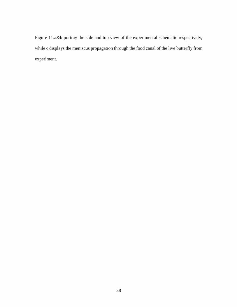
38

Figure 11.a&b portray the side and top view of the experimental schematic respectively,

while c displays the meniscus propagation through the food canal of the live butterfly from

experiment.

39

Figure 11. Experimental setup for proboscis separation and butterfly sedation. a) Side view of the setup where

the butterfly is shown with its wings in paper (shown by the transparent rectangle) and held together with a clothespin

(brown). The proboscis (black line extending off of the head of the butterfly) was extended and placed in a PDMS clamp

(not pictured) to ensure stability of the galeae. The butterfly was sedated by using dry ice in a warm water bath (beaker

on a hot-plate shown to right of the butterfly) to create a CO2 gas which flowed out of the tube (green) via a showerhead

40

configuration to surround the butterfly with the gas. After sedation the butterfly recovers completely within a few minutes.

b) Top view of the galea separation experiment where the blue regions between the galeae represent the saliva menisci

and the red signifies the separation post. c) Experimental frames of the separated galeae showing saliva propagation of

a butterfly in the “active” state, or before it has been dosed with CO2.

By glancing at Figure 11.c, it can be seen that there are liquid menisci to the left

(tip side) and right (head side) of the separation wire and one can glean that saliva has run

all the way to the tip and consequently filled the food canal. This can be said with

confidence due to the hydrophilicity of the interior of the food canal where a liquid finger

running along the interior surface of the canal must travel all the way down to the tip and

subsequently fill the canal; only afterwards can a liquid meniscus can be seen between the

galeae on both sides of the wire.

To determine if this phenomenon is prevalent in other butterflies, we tested

Monarchs (Danaus plexippus) and American Painted Ladies (Vanessa virginiensis) (56,

57) where, despite variability in size of the butterflies, shapes of the proboscises, and

feeding habits, we saw similar results between both types; henceforth, we can say that it is

common for butterflies to have the ability to completely wet their food canals with saliva.

Furthermore, when taking Figure 12.c into account, liquid pumping from the butterfly can

be observed; in the first frame at 0.00 s, there is no visible meniscus, but less than a second

later liquid can be seen on both sides of the wire, and finally, at 1.30 s, the meniscus has

receded on both sides.

We have seen another interesting phenomenon; some butterflies do not send liquid

down to the tip of their proboscis. The butterflies producing saliva can be observed

repairing their proboscis just minutes after the separation wire was withdrawn. However,

in some butterflies, no meniscus can be found and their proboscises are dry and inflexible

41

which, after putting in the experimental apparatus, running the test, and drawing the post

back to supposedly initiate repair, leads to a permanently separated and deformed

proboscis. This further supports our hypothesis that the saliva not only aids in the repair

of the proboscis, but seems to play an essential role in the self-repair of the galeae into one

component.

3.1.4.3 Butterfly Sedation

To say with confidence that the saliva of the butterfly plays a significant role in the

repair of the proboscis, we needed to separate the muscular forces from the capillary forces

acting upon the galeae in the repair process. To accomplish this goal, we used a CO2

sedation method (58) to minimize muscular action of butterflies (Figure 12.a). With the

exception of the addition of CO2, the second experimental procedure closely followed the

steps outlined in Chapter 3.1.4.2 where the galeae were separated by a post moving in small

steps. This additional step exploits the sublimation of CO2 from a solid form (dry ice) into

that of a gas by submerging pellets of dry ice into a warm water bath (~80 ˚C). The

resulting CO2 gas emissions were directed onto the head and body of the Lepidoptera for

the purpose of sedation by positioning the outflow opening of the tube towards the body of

the butterfly. This was specifically carried out when the saliva meniscus was close to, or

touching, the post so that a long liquid column could be seen and it was carried out until

the movement of the butterfly became inhibited, i.e., when there were no muscular actions

or hydrostatic deviations in the galeae from hemolymph (blood of insects) propagation.

Once no movements were visible, the butterfly was considered to be sedated. Afterwards,

42

the pressure produced by the butterfly onto the liquid column seemed to relax and the saliva

wanted to retract towards the head, a process that results in the further separation of the

galeae from which the effects of the capillary action can be gleaned. Thus, we are

investigating the inverse situation of repair by observing the galea deflection of the sedated

butterfly as the visible saliva meniscus is drawn away from the crack. The entire process

was filmed via the same camera and software that was mentioned previously, Chapter

3.1.4.2, to maintain consistent quality in the videos at a frame rate of 40 fps.

3.2 Data Acquisition and Analysis

3.2.1 Video Editing

VirtualDub video editing software was used for simple video modifications such as

cropping, rotation, and compression. To keep the videos consistent, we always used the

same procedure as follows. First, we opened the video in VirtualDub, we went to the

‘video’ tab, and opened up the ‘compression’ window where we chose the ‘XVid

compression codec’ with a target compression of 8 (between 0 and 20) which decreased

the file size of the videos and helped them run smoothly in the LabVIEW program. Lower

numbers for the target compression correspond to less compression and, therefore, a

smaller decrease in file size. After compression, we went to the ‘filter’ tab and added a

filter called ‘null transform’ which is a blank filter that doesn’t adjust the frames in any

way until we hit the ‘cropping’ button. In the ‘cropping’ window, we selected the region

of interest for the video by adjusting the height and width of what was shown in each frame;

however, each quantity must be a product of four due to the compression algorithm used

43

in the XVid Codec. Post cropping, we went through the video and separated it into three

parts; awake, sedating, and sleeping which correspond to regions in the video where the

butterfly can be seen moving and pumping saliva between the galeae, where CO2 gas can

be seen moving across the camera and less movement occurs, and where there is no

muscular action at all, i.e. the butterfly is completely anesthetized, respectively. These

three segments were saved as separate video files with names matching their region in the

video for easy identification later on in analysis. Once all of the segments were identified

and saved, a new video was opened and the steps were repeated.

3.2.2 LabVIEW Video Analysis Algorithm

After successfully acquiring the experimental videos, we were met with the task of

analyzing the frames in the videos by rotating the images so that the galeae were horizontal,

determining the angle at which the galeae touched the post, and extracting the profiles of

the galeae as X-Y coordinates. To do this, we created a custom code in National Instruments

LabVIEW®, using many features from their Vision Development Module, and paired it

with an analysis code developed in Wolfram Mathematica®. The data flow can be seen in

Figure 12 below where the green boxes correspond to steps done in LabVIEW (outlined

below) and the red ones relate to tasks completed in Mathematica (described further in

Chapter 3.2.3).

44

Figure 12. Flow-chart displaying data flow between LabVIEW (green) and Mathematica (red) to outline the general steps used in video/data analysis. The steps for LabVIEW analysis can be found in this chapter, but those used for data analysis in Mathematica can be found in Chapter 3.2.3.

The image processing procedure is as follows. First, we imported a video file by

adding the desired file path to an input text string which was fed into IMAQ AVI2 Open

and then to IMAQ AVI2 Get Info. This opens the video and gives information on each

image such as the number of frames and image size.

Once the video has been imported, it was directed into an IMAQ Create where we

created a mirror of a frame in the video and turned the RGB frames into grayscale for easier

processing. Even though the frames were grayscale, they were still complicated by

undesired artifacts such as a non-uniform background, the presence of the post behind the

galeae, and other foreign objects due to the lack of controlled environment. Therefore, a

set of binary (black and white) images was created via the IMAQ Local Threshold to deal

with image complications and the window size for the threshold was left adjustable to best

visualize each frame.

45

To gather the profiles of each galea in steps further down the road, the images had

to be broken up into two adjustable rectangular regions of interest (ROI). One rectangle

was used for each galea (stacked on top of each other) which spanned the entire horizontal

length of the image. After creating a series of binary images composed of pixel values of

0 (black) and 255 (white) and creating the ROIs, these images were then rotated so that the

proboscis was aligned as horizontally as possible.

Next, a contour line was created for each ROI by using the IMAQ Extract Contour

algorithm and the direction of the contour search was set to top-to-bottom for the top galea

in the image and vice-versa for the bottom galea. This contour algorithm finds the first

largest length of contrast in each ROI, the external wall of each galea in this case, and maps

them with contour lines so that the coordinates of the lines can be used to create plots for

each individual galea. An example frame of the grayscale and binary, contoured images

can be seen in Figure 13.

Figure 13. a) Original, sample image of the butterfly proboscis which had been split by a tungsten wire and b)

the binary (black and white) image with contours (thick green lines) on the exterior of the proboscis and the regions of

interest shown by the thin green rectangles situated at an angle parallel to the length of the proboscis.

46

Next, the extracted coordinates of the profiles were normalized by the quantity

( )gR T consisting of the post radius and the thickness of a galea at the post, which were

both manually measured parameters for each video. Likewise, we manually measured the

air gap between the meniscus front and the middle of the separation post, lairgap. The

rightmost point of this line (typically at the middle of the wire) was used as a cutoff point

in the coordinates so that the normalized profiles only go up to the center of the post and

therefore only extend to 1 on the Y-axis. The thickness of a galea at this point had to be

introduced since the contours used were those of the exterior walls of the galeae; had we

not done so, the profiles normalized by the post radius would’ve extended well past 1 and

fitting would not have been possible. Once doing so, we were left with profiles of the top

and bottom galeae, which could then be fitted by the solutions, [21] and [22].

In Figure 13, one can see the transition from grayscale to the binary, contoured

image, which is necessary to gather data in future steps. However, in many of the frames

(especially for active butterflies), the galeae deflections were not symmetric relative to the

neutral axis between them (shown by the interface between the top and bottom regions of

interest, thin green lines, in Figure 13.b). Furthermore, the galeae often touch the post at

positions before or after the center of the separation post leaving the galea at a tangent

angle other than 2

. Therefore, it was necessary to extract the slope of the tangent line

between the galea and the post. This was done by taking the rightmost coordinate points

(found from the contours), fitting them with a linear line, and then taking the derivative of

that linear line. We then realized that there were three scenarios of galeae shape that had

47

to be taken into account and dealt with differently in order to gather the correct angle θ

(Figure 5).

The first case is the one where the galea is laying on the post completely parallel

with the X-axis; as such, the tangent angle θ is perpendicular to the horizontal axis, or

2

and 0

dY

dX .

The second case was defined as the situation in which 2

and, in such a case,

the slope of the galea at the post is 0dY

dX . Now defining angle 1 as 1 arctan

dY

dX

and using simple geometry we can see that 12

and hence, we are left with:

arctan2

dY

dX

[31]

where dY

dX is our measurable parameter from the experimental videos. Thus, our tangent

angle θ for case 2 has been defined by [31]. By following similar methods for case 3 where

2

and therefore 0

dY

dX . The 1 arctan

dY

dX

condition still applies, but here we

must establish new angles 2 and which are shown in Figure 9. The former can be

defined as 2 arctandY

dX

while the latter can be found as

2 arctan2 2

dY

dX

and, thus, we can find the tangent angle for this case as

shown by [32] below.

48

3

arctan2

dY

dX

[32]

Once all of the necessary experimental parameters have been measured, namely

lairgap and θ, a text string was created that included all of the important values along with

the video name and frame analyzed for identification purposes. Then the normalized

profile coordinates were exported as a spreadsheet file with the previously created text

string as the file name. This file was then opened with a custom Wolfram Mathematica®

program for further analysis.

3.2.3 Mathematica Data Analysis

The main goal for the Mathematica program was to use our mathematical model to

analyze the normalized profiles that were extracted from the experimental videos via

LabVIEW. The data flow in this program can be briefly described by Figure 12, but is laid

out in detail as follows. First, the normalized equations [14] and [15] were inputted along

with the set of boundary and continuity conditions shown by [16]. Then, two derivatives

of [14] and [15] were taken for use with the boundary conditions. Then, the first two

boundary conditions in [16] were used to solve for two of the integration constants for [18]

. Additionally, the next two boundary conditions were used to solve for two of the

integration constants in [20]. Thus, we were left with four integration constants and can

use the four remaining continuity conditions in [16] to solve for them. The Solve function

in Mathematica was used for all of the analytical solutions. Next, a piecewise function was

49

created and the analytical solution of [21] was set to be used in the domain 0 X l , the

portion of the galea described by Zone 1, while [22] was used from l X L .

Now that the piecewise function describing the galeae along the length of the

proboscis was created, we can analyze the experimental data. First, we had to import the

extracted coordinates (created in LabVIEW) into Mathematica and save all of the

experimental parameters (present in each experimental filename) as certain parameters in

Mathematica. Then, after inputting all of the experimental parameters into the theoretical

piecewise solution, the FindFit command was used to fit the experimental curve and gather

B which could later be used to calculate the flexural rigidity D of the proboscis. This

FindFit algorithm numerically minimizes the sum of residuals squared, which is a

summation of the differences between the experimental and theoretical deflection over all

data points, i, 2

exp th

i i iY Y where exp

iY and th

iY are the experimental and theoretical

deflections at point i. However, one difficulty we had here was that the length of the crack,

L, is moveable and unknown and therefore, we were left with a moving boundary problem.

Thus, we needed to create a numerical, iterative technique using the previously gathered B

parameter as the initial fitting value and the largest value in our coordinate array as the

preliminary L. This is possible since the deflection in Y(X) is normalized by R and hence,

the largest value in the array will always be the length of the galea up to the post. After

this we could start the iteration process with L as our iterative term and [17] as our iterative

condition to be met in the While loop. Depending on the accuracy of the first fit, we could

adjust the iteration step according to the distance required to create a better fit. However,

we usually gathered accurate fittings (R2>.95) with our initial fitting method, so when

50

running our data in the iterative process we would receive values that are the same as with

the initial; therefore, we only used the iterative process when necessary, for instance, when

the initial fit was poor. Through these means, we’ve collected all of the data in Chapter 4.

51

CHAPTER FOUR

RESULTS AND DISCUSSION

4.1 Materials Properties of the Butterfly Proboscis

4.1.1 Saliva Movement Paradox: Where does the saliva go when receding at the tip?

During this experiment, a saliva meniscus can be seen on each side of the post

indicating that it travels to the tip prior to the splitting of the proboscis. After separating

the galeae, saliva gets trapped on the tip-side (Figure 11.c) and a meniscus can be seen

propagating back and forth. However, when the butterfly is sedated, the saliva meniscus

can be seen retracting towards the tip, which creates the following questions: why does the

saliva move to the tip and is there some reservoir where the saliva can move? If so, is this

reservoir a feature of the proboscis, similar to a pore, or is the saliva moving elsewhere?

To answer these questions, we modified the previous experiment described in

Chapter 3.1.4. The experiment remains largely the same in that the butterfly was placed in

the holding apparatus, the proboscis was straightened out, and the tip was placed in the

PDMS clamp; however, the main difference here is that the proboscis was not split.

Instead, the enclosed tip was brought under the same PointGrey camera and focused on

through the transparent PDMS. After carrying this out, almost immediately the saliva was

seen leaving from the tip region of the proboscis and moving into the small opening

between the PDMS layers. This process is illustrated in Figure 14. This simple experiment

demonstrated that the saliva withdrawal from the post at the tip side of the proboscis is due

to capillary wicking of the saliva between the two PDMS layers, and thus, we conclude

that the reservoir we were searching for was actually the gap in the PDMS clamp.

52

Figure 14. Displaying the escape of saliva from the tip of the proboscis and its propagation inside of the PDMS

clamp over time. The video was recorded at 30 FPS.

This saliva propagation into the PDMS clamp piqued our interest and led us to study

the kinetics of these snapping-off moments in the videos of sedated butterflies further due

to the supposed correlation between the two. To do so, we used the custom LabVIEW

software to measure the air gap between the center of the post and the meniscus front for

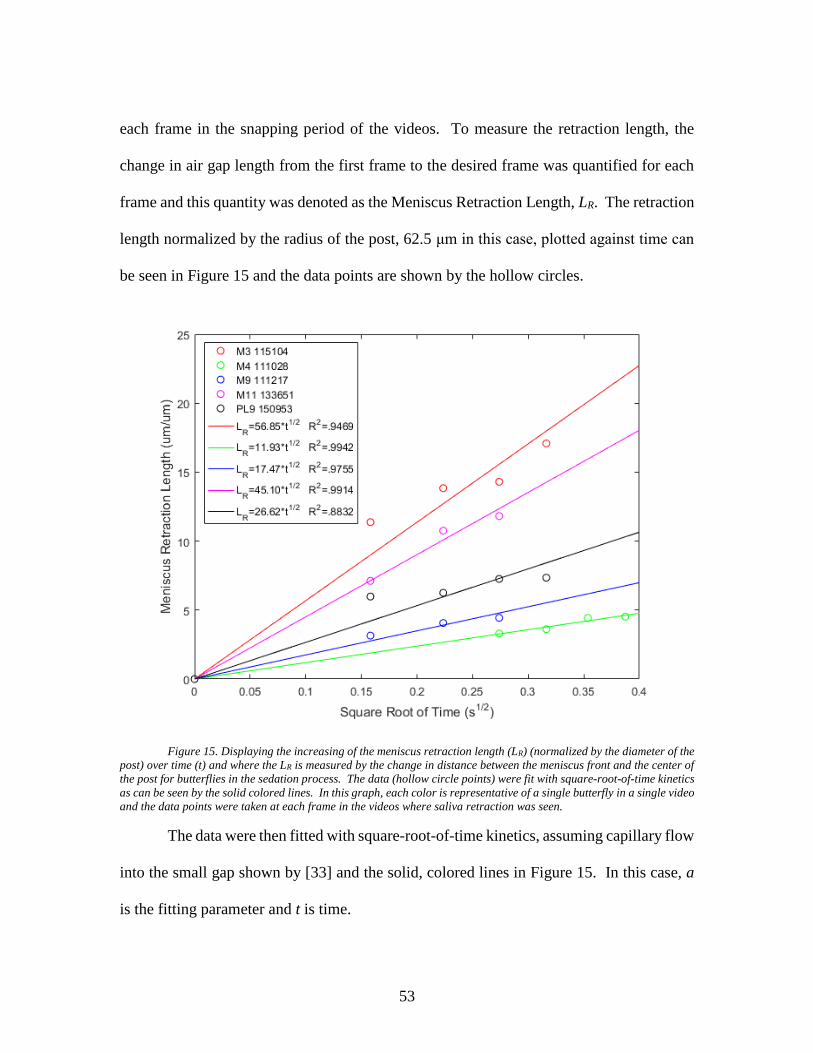
53

each frame in the snapping period of the videos. To measure the retraction length, the

change in air gap length from the first frame to the desired frame was quantified for each

frame and this quantity was denoted as the Meniscus Retraction Length, LR. The retraction

length normalized by the radius of the post, 62.5 μm in this case, plotted against time can

be seen in Figure 15 and the data points are shown by the hollow circles.

Figure 15. Displaying the increasing of the meniscus retraction length (LR) (normalized by the diameter of the

post) over time (t) and where the LR is measured by the change in distance between the meniscus front and the center of

the post for butterflies in the sedation process. The data (hollow circle points) were fit with square-root-of-time kinetics

as can be seen by the solid colored lines. In this graph, each color is representative of a single butterfly in a single video

and the data points were taken at each frame in the videos where saliva retraction was seen.

The data were then fitted with square-root-of-time kinetics, assuming capillary flow

into the small gap shown by [33] and the solid, colored lines in Figure 15. In this case, a

is the fitting parameter and t is time.

54

1/2

RL t at [33]

As one can see in Figure 15, we have good agreement between theory and

experiment, which validates our hypothesis that capillary wicking of the saliva into the gap

in the PDMS clamp from the liquid column near the tip does occur. However, the wicking

of the saliva does not occur at constant rates as can be seen by the wide distribution of data

as well as their respective fitting parameters (shown in front of the t1/2 in the legend inside

of Figure 15). This mystery will not be addressed in this work.

4.1.2 Results from Data Fitting and Mechanical Testing of Galeae

After the video analysis was completed, we performed the data fitting with the

solutions [21] and [22] to gather the desired materials parameters of the butterfly proboscis,

which lie in our fitting parameter B. The data fitting algorithm is a multiple step process

that can be found described in Chapter 3.2. Figure 16.a-c shows a variety of satisfactory

fits for the curves extracted from butterflies undergoing the sedation process (shown in

blue data points). The shape of the sedated butterfly’s proboscis did not change much

between frames due to the lack of muscular action; this lead to relatively unchanging

profiles between frames. However, the shape was different between the bottom galea and

the top galea due to the asymmetry of the galeae with respect to the neutral axis. Due to

this asymmetry, we have left these data out of the final data set, but they are still useful for

illustrating the robustness of our model.

55

Figure 16. Butterflies undergoing sedation process: a) M213 141820 Sedating BG Frame 123, b) M213 141820

Sedating TG Frame 142. Video 2: c) M213 141820 Sedating BG Frame 124. Active butterflies: d) M12 120131 Awake

BG Frame 0, e) M12 120131 Awake TG Frame 14,and f) M18 170354 Awake BG Frame 301.

Now that we have discussed the sedated butterflies, we can move on to a more difficult

scenario, at least in the data fitting sense, when the butterflies are active. The butterflies

are considered active when little or no CO2 has been used to sedate them and the proboscis

is twitching or moving in the videos. These deviations in contour profile led to difficulties

in data fitting, particularly because muscular action in the proboscis prevents the galeae

from having the desired shape as established by the Euler-Bernoulli beam model. For

instance, if the slope of the galeae at the start of the fitting region (left side) is not close to

zero, as our boundary conditions require, or if the butterfly manually separates the galeae

in the middle of the fitting region, we will have difficulty in getting a satisfactory match

between the data and the fit. With that said, in frames where the butterfly does not seem

to apply large muscular forces, we can see agreement between the experimental and

theoretical profiles as shown by the green data points in Figure 16.d-f.

56

Next, we must discuss the variability of the B parameter found for both species of

butterflies tested and the state that they were tested in (active, sedating, and sleeping). The

average B values from each butterfly in all three states can be found in Figure 17.

Figure 17. Displaying the average B values for Monarchs (shown in orange and M on the legend) and Painted

Ladies (shown in purple and PL on the legend) in the active state (A on legend), sedating state (Se), and sleeping

(anesthetized) state (Sl). It can be seen by the error bars overlaying the data bars that for the case of active butterflies,

there is much more variability than there is for sedated butterflies. Also, it is worth noting that TG and BG signify Top

Galea and Bottom Galea, respectively.

In this set of bar graphs, one can see the B values found for each particular butterfly

species and number, video number, and galea (top or bottom). The Monarchs are shown

by the orange bars and the Painted Ladies are shown by the purple bars. At this point it is

also worth clarifying how the legend can be read. As an example, let us choose the first

item on the legend (from top to bottom), namely ‘M213 143514 Se TG’. In this line of

text, ‘M213’ represents Monarch #213 that was tested, ‘143514’ is a string of numbers

generated by the video camera when acquiring a video for this particular butterfly and is

used for video identification purposes, ‘Se’ indicates that the butterfly was being sedated

0.00

0.05

0.10

0.15

0.20

0.25

Fit

tin

g P

ara

met

er (

B)

[Un

itle

ss]

M213 143514 Se TG

M8 145056 A TG

M11 133651 A TG

M4 110142 A TG

M8 134640 A BG

M1 142413 Sl BG

M4 114756 Sl TG

M9 144505 Sl TG

PL1 104827 Sl BG

PL1 134856 Sl BG

PL3 113156 A TG

PL3 113813 A TG

PL3 114723 A TG

PL6 154513 A TG

PL6 155022 A TG

PL1 134856 A TG

PL4 132734 Se TG

PL5 145450 Se BG

57

in this video, and ‘TG’ states that the top galea was tested (Figure 17). In this figure, it can

easily be seen that active, sedating, and sleeping (fully anesthetized) butterflies of both

species, Monarchs and Painted Ladies, span about an order of magnitude, from B=.07~.19,

which means that we can use this model for sedated butterflies as well as active ones.

However, the variability of active butterflies is much greater than that of sedating or

sedated butterflies. For instance, if observes the two sets of data, one awake butterfly, M11

133651 A TG, and one anesthetized, PL1 104827 Sl BG, the standard deviations of the B

for the awake butterfly is about twice the size of the standard deviation for the sleeping

butterfly. This is possibly due to the changing muscular actions inside of the proboscis for

the active butterfly and therefore the dm/dx which was previously ignored (Chapter 3.1.2)

would have to be taken into account in further iterations of the model. Furthermore, the

overall average B including both Monarchs and Painted Ladies was Boverall=.1520 with a

standard deviation of .0161 while the average B for Monarchs and Painted Ladies were BM

=.1519 and BPl =.1520 with standard deviations of .0148 and .0171, respectively. All table

of collected B values and standard deviations can be found in Table 2 below.

Table 2. B values (data shown in Figure 17) collected for each butterfly with their corresponding standard

deviations. The standard deviations were found by considering each video and taking measurements of B frame by frame.

In this data set, 6 Monarchs and 5 Painted Ladies were tested to make up the 8 and 10 videos tested for each species,

respectively. All other collected data can be found in the appendices.

Monarch B Painted Lady B

M213 143514 Se TG 0.20 PL1 104827 Sl BG 0.16

Standard Deviation 0.01 Standard Deviation 0.01

M8 145056 A TG 0.14 PL1 134856 Sl BG 0.14

Standard Deviation 0.02 Standard Deviation 0.02

58

M11 133651 A TG 0.17 PL3 113156 A TG 0.15

Standard Deviation 0.03 Standard Deviation 0.01

M4 110142 A TG 0.14 PL3 113813 A TG 0.16

Standard Deviation 0.03 Standard Deviation 0.01

M8 134640 A BG 0.11 PL3 114723 A TG 0.17

Standard Deviation 0.01 Standard Deviation 0.01

M1 142413 Sl BG 0.18 PL6 154513 A TG 0.19

Standard Deviation 0.00 Standard Deviation 0.03

M4 114756 Sl TG 0.13 PL6 155022 A TG 0.18

Standard Deviation 0.00 Standard Deviation 0.02

M9 144505 Sl TG 0.15 PL1 134856 A TG 0.16

Standard Deviation 0.01 Standard Deviation 0.02

PL4 132734 Se TG 0.14

Standard Deviation 0.02

PL5 145450 Se BG 0.15

Standard Deviation 0.03

Monarch Average 0.1519 Painted Lady Average 0.1520

Standard Deviation 0.0148 Standard Deviation 0.0171

Overall Averages 0.1520

Overall Standard Deviation 0.0161

Now that the non-dimensional B values have been found from fitting, we can

calculate the Longitudinal Young’s Modulus of Elasticity E of the galeae for Monarchs

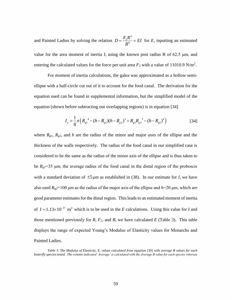
59

and Painted Ladies by solving the relation 4

2

4

F RD EI

B for E, inputting an estimated

value for the area moment of inertia I, using the known post radius R of 62.5 μm, and

entering the calculated values for the force per unit area F2 with a value of 11010.9 N/m2.

For moment of inertia calculations, the galea was approximated as a hollow semi-

ellipse with a half-circle cut out of it to account for the food canal. The derivation for the

equation used can be found in supplemental information, but the simplified model of the

equation (shown before subtracting out overlapping regions) is in equation [34]

4 3 3 4

1 1 2 1 2 1

1( )( ) ( )

8y g g g g g gI R h R h R R R h R [34]

where Rg1, Rg2, and h are the radius of the minor and major axes of the ellipse and the

thickness of the walls respectively. The radius of the food canal in our simplified case is

considered to be the same as the radius of the minor axis of the ellipse and is thus taken to

be Rg1=35 μm, the average radius of the food canal in the distal region of the proboscis

with a standard deviation of 5 μm as established in (38). In our estimate for I, we have

also used Rg2=100 μm as the radius of the major axis of the ellipse and h=20 μm, which are

good parameter estimates for the distal region. This leads to an estimated moment of inertia

of 17 41.13 10 mI which is to be used in the E calculations. Using this value for I and

those mentioned previously for R, F2, and B, we have calculated E (Table 3). This table

displays the range of expected Young’s Modulus of Elasticity values for Monarchs and

Painted Ladies.

Table 3. The Modulus of Elasticity, E, values calculated from equation [30] with average B values for each

butterfly species tested. The column indicated ‘Average’ is calculated with the Average B value for each species whereas

60

the ‘Low Estimate’ and ‘High Estimate’ are calculated with the upper and lower B values that would be found based on

our standard deviation respectively. For further clarification, higher B values lead to lower E values.

MODULUS OF ELASTICITY (E) [MPa] – Tip

Butterfly Species Average Low Estimate High Estimate

Overall 27.88 18.63 43.66

Monarch 27.96 19.28 42.14

Painted Ladies 27.83 18.18 44.81

Now, one can compare the calculated E values for Monarchs and Painted Ladies to

those found by tensile testing. A Dynamic Mechanical Analyzer (TA Instruments© DMA

Q800-0907) was used for tensile testing experiments with the help of the MS&E materials

characterization expert, Kim Ivey. The DMA was run in a controlled strain rate mode

(0.25% strain/min to 25% at temperature of 22˚C) where it simulated an ordinary tensile

test by extending a sample and measuring the resulting force until the sample fractures or

slips out.

These experiments were run on dead butterflies (usually no longer than two days

after they perished) and the galeae were separated, similarly to how it was described in

Chapter 3.1.4, severed from the head of the butterfly, and then the tip of each galea was

placed in an epoxy putty (J-B WELD® PlasticWeld™ or SteelStik™, succeeded with both)

that was attached to a plastic clamp with flat external surfaces to prevent slippage of the

sample during testing. During testing, the sample typically extended to between 1% and

3% strain before breakage occurs. All DMA data can be found in the appendices. Figure

18 shows a sample of the data taken from DMA.

61

Figure 18. Modulus of Elasticity values taken from DMA tensile testing. This bar graph follows previous

conventions; orange represents monarchs tested, purple represents the painted ladies tested, and the green represents

the average modulus of all butterflies tested with an error bar showing one standard deviation above and below the

average. The legend can be read as such; M stands for Monarch and PL stands for Painted Lady, the number afterwards

represents the number of butterflies tested, and A or B signifies the galea that was tested from that butterfly.

When comparing the results from our method to the DMA, one can see that our

estimations from curve fitting are an order of magnitude greater than that of the DMA.

There may be two possible reasons for this: 1. The butterfly tested in our galea separation

experiment is thought to have had an internal pressure created by the hemolymph (blood

of butterflies) that flows inside the proboscis. This internal pressure is also thought to

increase the rigidity of the galeae and thus, the effective modulus of elasticity that is

measured by our experiment would also increase. In the DMA experiments, we were

testing proboscises that were severed from the head of the dead butterfly and the

hemolymph was dry, so we did not have any pressure from the hemolymph. Measuring

the pressure inside the galeae is not in the scope of this work, so this question will remain

unanswered. 2. The modulus E calculations from our data fitting with B are sensitive to

62

the moment of inertia I that is inputted into the equation 4

2

4

F RE

B I , so since we are using

parameters for the moment of inertia that are found near the distal region (or tip) of the

proboscis, it would make sense that E would be larger than what is experienced with

experiments. Therefore, if we were to use typical parameter values that can be found in

the knee region (middle of the proboscis), we should be able to increase I and thus decrease

E to garner better agreement between our theoretical results and mechanical testing. These

parameters can be found in Table 5. Additionally, new estimations for E with the moment

of inertia near the middle of the proboscis can be found in Table 4.

Table 4. Comparison between the Modulus of Elasticity E values found from the theoretical curve fitting and

the mechanical testing after calculating the moment of inertia with parameter values for Rg1, Rg2, and h found near the

middle of the proboscis. Values for these parameters can be found in Table 5. This table shows that when using shape

estimates for the galeae near the middle of the proboscis instead of the tip, we find much better agreement between our

theory and mechanical experiments in both the averages and the lower and upper bounds (when using one standard

deviation to calculate them).

MODULUS OF ELASTICITY (E) [MPa] – Middle

Butterfly Species Average Low Estimate High Estimate

Overall 3.14 2.10 4.92

Monarch 3.15 2.17 4.75

Painted Ladies 3.14 2.05 5.05

MODULUS OF ELASTICITY (E) [MPa] – DMA

Average 4.13 2.24 6.03

As one can see from Table 3, the calculated E values of the butterfly proboscis for

both Monarchs and Painted Ladies are similar, and when calculated with an I near the

middle of the proboscis, are in agreement with the values from tensile testing with the

DMA and thus, we can glean from these data that the pressure of the hemolymph inside

the galeae does not play a large role in the stiffness of the organ. For reference, this range

of E values (under 10 MPa) is a few orders of magnitude lower than that of human hair,

63

which has an average value of about 3 GPa based on Quan’s observations (59). Therefore,

based on our calculations, we can say that in nature these butterflies, Monarchs and Painted

Ladies, do not need a rigid proboscis for drinking nectar from flowers and actually, the

flexibility of the proboscis facilitates the coiling and uncoiling needed for feeding as well

as the assembly/repair process. However, there are butterflies with much shorter or longer

proboscises than those studied here and these butterflies may need a more rigid proboscis

for purposes such as insertion into narrow flower tubes. The parameters used in the

modulus of elasticity calculations can be found tabulated in Table 5 below.

Table 5. Tabulated parameters used in modulus of elasticity E calculations where the symbol is shown in

parenthesis and the corresponding units are shown in brackets.

FITTING PARAMETER (B) [Unitless]

Butterfly Species Average Standard Deviation

Overall 0.1520 0.0161

Monarch 0.1519 0.0148

Painted Ladies 0.1520 0.0171

OTHER PARAMETERS USED IN CALCULATIONS

Parameter Name and (Symbol) Values used in

calculations [Units]

Radius of the separation wire (R) 62.50 [μm]

Force Per Unit Area (F2) 11010.90 [N/m2]

Tip – Distal Region of Proboscis

Moment of Intertia (Iy) 171.13 10

[m4]

Radius of the Minor Axis of the Ellipse

(Rg1) 35.00 [μm]

Radius of the Major Axis of the Ellipse

(Rg2) 100.00 [μm]

Wall Thickness (h) 20.00 [μm]

Middle – Knee Region of Proboscis

Moment of Intertia (Iy) 16

1.00 10

[m4]

Radius of the Minor Axis of the Ellipse

(Rg1) 40.00 [μm]

Radius of the Major Axis of the Ellipse

(Rg2) 200.00 [μm]

Wall Thickness (h) 27.00 [μm]

64

4.1.3 Adhesion Forces Between the Galeae

The galeae separation experiment was first designed to determine the mechanical

properties of the butterfly proboscis, but by investigating the shear forces in the galea, or

beam, along its length, we can actually gather the normal force created by the contact

between the galeae and the post and consequently determine the adhesion forces at the

crack location between the galeae and the capillary forces bringing them together. Most

of the forces are acting in the orders of magnitude between mN and μN, which is what was

expected for fibers of such small size, capillary forces, and small deflection of the galeae

from the post. Additionally, when looking at the capillary force data, as the meniscus

length l, or the length of the wet region, increases, we have an increase in magnitude of our

capillary force, which can be seen in Figure 19. The capillary force, Fc, was found from

an integration of forces from the crack position (X=0) up to the meniscus; therefore, all

capillary forces in our experiment were taken into account. These calculations can be

found in Chapter 3.1.2.5.

65

Figure 19. Displaying the Capillary force (Fc) against the length of the wet region along the length of the

galeae. As capillary length increases, we have a corresponding increase in magnitude of capillary force and, thus, a

greater restoring force. In this figure, the orange and purple dots represent data from Monarchs and Painted Ladies,

respectively. Additionally, the error bars in the x and y directions are showing one standard deviation for each of the

data points. The larger error bars correspond to tests on active butterflies while those with smaller error bars are

typically sedated or sleeping butterflies. The linear trendlines were added to guide the eye as to how the data was acting.

This raw data can be found in supplemental information.

Now we can introduce the adhesion force in the horizontal and vertical directions

with Figure 20. These forces were gathered from the shear force profile along the length

of the beam (third derivative with respect to displacement) and these calculations can be

found in Chapter 3.1.2.

66

Figure 20. Adhesion forces plotted against θ in the a) Horizontal direction (Vadx) and b) Vertical direction

(Vady). In these figures, orange and purple dots correspond to tests with Monarchs and Painted Ladies, respectively.

Error bars use the same conventions as in previous figures.

The horizontal adhesion force data shows a noteworthy trend (Figure 20.a). As θ,

or the angle between the normal vector at the point of contact between the galea and post

and the axis of symmetry goes to π/2 (~1.57 radians), the horizontal component of the

adhesion force diminishes to zero and actually, as the angle surpasses π/2, we get negative

values. This is displaying exactly what was expected for the three cases that were

67

mentioned previously. For instance, at angles below π/2, our horizontal adhesion force is

pointing towards the post and thus creating a compression scenario in the beam. On the

contrary, for angles above π/2, we see a reverse in the sign showing that the force is acting

in the opposite direction and thus, the case has switched to the tensile scenario. Likewise,

in between these two cases, we are left with extremely small adhesion forces that tend to

zero as we get closer and closer to π/2; and therefore, we have only vertical components of

the forces in this case as expected.

The vertical adhesion data is not easy to interpret (Figure 20.b). It was conjectured

that as θ tended to π/2, we would see an increase in vertical adhesion forces due to the

horizontal component going to zero. This is not the case for a couple of reasons. First,

since the vertical component is at least an order of magnitude larger than the horizontal

component in most of our cases, the increase in vertical force from the decrease in

horizontal force as the angle moves towards π/2 would be much smaller than that of the

original vertical force and thus, the deviation would not be noticeable in our data. Second,

since the profile of the proboscis is unique in every video and the vertical adhesion force

is directly related to this profile, it is likely that we would have a scatter of data due to this

and, thus, we do not have any direct trends between our vertical adhesion force and θ.

However, the range of vertical adhesion data points lie between 0.09 mN and .25 mN

(Figure 20.b), which coincidentally sits in the range exhibited by the capillary force data

points between .15 mN and .35 mN (Figure 19), but is always less than its corresponding

capillary force. This, along with the presence of liquid saliva and lack of other external

stimuli, suggests that the adhesion is most likely caused by capillarity.

68

CHAPTER FIVE

CONCLUSIONS

In this work, we have successfully created an adhesion characterization method

founded on the concept of Euler-Bernoulli Beam Theory and the treatment of fibers,

namely the lepidopteran galeae, as beams undergoing small deflections. We developed an

experimental protocol that enabled a quantitative analysis of capillary adhesion between

complex-shaped fibers of living organisms that can be extended to man-made fibers. We

developed a code in LabVIEW for the image analysis and contour fitting/extraction of the

galeae profile for use with the mathematical model. Alongside the LabVIEW code, a data

analysis code was developed in Mathematica which found solutions to the Beam Theory,

imported the contour data, and fit the data with the theory.

To find the adhesion forces holding the galeae together, we have taken the third

derivatives of the deflection solutions for each butterfly to determine the shear forces acting

on the galeae along its entire length. Then we investigated the shear force at the crack

location between the galeae (X=0) and at the position of contact between the galeae and

the wire, point A’, to determine the vertical adhesion force Vady in the beam acting to keep

the galeae together and the normal force Fn at the post acting to separate them.

Furthermore, we have found the capillary force acting to bring the separated galeae back

together by integrating the distributed force from the crack to the meniscus location.

Finally, we have found a horizontal adhesion force acting on the beam with a force balance

since the angle between the neutral axis and normal vector at the point of contact between

69

the galea and the wire is not always π/2; thus, we have exposed the horizontal forces acting

on the beam in the compression and tension states.

The measured vertical adhesion force is on the same order of magnitude as the

capillary forces found through integration along the meniscus length, which indicates that

the adhesion is due to capillarity and that capillary forces play a significant role in bringing

the galeae together and keeping them together in the repair and assembly processes.

Although the adhesion forces are feasible and the data exhibit the expected trends, it still

requires a secondary experiment for validation purposes to ensure that the data are correct;

however, this is a point of discussion for another work and an experimental method for

carrying this out along with some preliminary results can be found in Chapter 6.

Additionally, we have extracted the Young’s Modulus of Elasticity E of the

lepidopteran proboscis (for Monarchs and Painted Ladies that were active, being sedated,

and sleeping) from the profile of the deflected butterfly galeae by using Euler-Bernoulli

beam theory to relate the shape of the galea or ‘beam’ with the shear and moments acting

on it. The modulus was around 3.14 MPa for Monarchs and 3.15 MPa for Painted Ladies

based on data from video analysis and curve fitting using our solutions to the differential

equations in this theory and an estimation for I (taken from the knee region of the

proboscis). These data were corroborated with the moduli found from the tensile testing

of the butterfly galeae via DMA, which yielded an average modulus of 4.13 MPa between

species. Although we had good agreement between the DMA and the E values found from

B-fittings, we cannot confidently say the extracted moduli are correct due to our simple

approximation of the galeae shape (I), the lack of knowledge about F1 and F2 in [5], and

70

the assumption that E and I are constant along the length of the beam which is inherent in

this type of beam theory; however, as was mentioned previously, the proboscis shape is

tapered along its length and thus, it should not have a constant I. The further study of E

and I of the lepidopteran proboscis is the point of discussion for another work.

71

CHAPTER SIX

SIGNIFICANCE OF WORK

In this work we successfully determined the modulus of elasticity of a complex bio-

fiber known as the butterfly galea by using Euler-Bernoulli beam theory to relate the shape

of the fiber with the moments acting on the beam and the materials properties of the beam.

Also, we have created an adhesion characterization method based on this beam theory that

works by investigating the shear forces inside the beam and using force balances of the

galea free-body diagram to determine the horizontal and vertical components of the

adhesion force. This method, when validated with another experiment or force transducers

(to directly measure the applied force on the beams and wire), could potentially be used for

a wide range of composite materials such as fibers embedded onto/into matrices. Since

there is a plethora of adhesion characterization methods that do not produce repeatable and

easily analyzable results, we suggest there is a great need for a new adhesion experiment

and that this new method based on the shape of a deflected fiber could possibly help to fill

in that void. Therefore, to show that this method can be extended to other non-biological

materials, we have done a preliminary investigation with well characterized, tungsten

fibers.

6.1 Reference Adhesion Experiment using Ribbons of Well-Characterized Materials

6.1.1 Experimental Motivation

The goal of this reference experiment is to recreate the setup made for the butterfly

proboscis, but with other, non-biological fibers instead. This will help to validate the

72

method and display that with a well characterized material such as tungsten, which has a

modulus of elasticity of abound 400 GPa, fiber deflection via capillary forces can still be

realized and this deflection can be used as a measure of adhesion forces. This would also

show that our model isn’t limited by the rigidity of the materials being tested and that our

model can extract the materials properties from more stiff materials as long as they’re in

the same experimental configuration. Additionally, in the future when adding a force

transducer to various points on the fiber/setup, we will be able to determine the adhesion

forces in the horizontal and vertical directions and relate them with what is being measured

via our deflection method.

6.1.2 Experimental Protocol

To produce an experiment that is a reliable means of determining the materials

parameters from these complex, biological fibers, we must have a reference fiber to

validate our findings with the proboscis. We have mimicked the setup of the galeae

separation experiment with ribbon-like fibers. With ribbons there are two flat sides with

an edge in between that prevents droplets from moving from one flat surface to the other

due to the pressure singularity at the edge. Thus, to simulate the proboscis experiment, we

have used two ribbons of similar length to the proboscis (between 3 and 4 cm) and have

placed them together such that one face of each is touching the other. Then we have taped

both ends together with single sided scotch tape so that they stay together near the edges

but can be separated in the middle. The taped ends were placed in two clothespins that

were attached to a wooden block such that the fibers are straightened out (Figure 21.a).

73

Figure 21. Experimental setup for the reference experiment. a) Side view of the experiment showing the wooden

clothespins, the syringe holder, syringe, and 90˚ angled needle used to send water between the ribbons, the 500 μm

separation tungsten wire (shown by the vertical wire in the middle), the tungsten ribbons (shown by the horizontal

metallic strip), and the tape holding them together at the ends. b) Top view of the experiment showing the top edge of

the ribbons which have been separated by the wire (500 μm).

Next, the fibers were separated by a tungsten wire of known diameter, which was

attached to a 2-D manipulator so that different profiles could be realized (Figure 21.b).

Following the separation of the ribbons, the camera was used to take a few images to be

used as reference images before moving to the next step, the placement of a controlled

amount of liquid between the ribbons to mimic saliva propagation. Liquid had to be used

to measure the modulus of elasticity of the materials because when looking back to our

differential equation for the dry region [15], the EI drops out of the equation and we are

left with a polynomial solution [20].

To successfully place controlled amounts of liquid between the ribbons, we used a

specialized setup including a syringe (Cadence Science, inc. 1 mL Glass Tuberculin

Syringe), syringe holder with adjustable knobs to produce droplets (disassembled from

74

Krȕss DSA10), and 90˚ angled needle (EFD SS Tip 15 Gauge Blue) which were combined

appropriately and positioned horizontally and perpendicular to the ribbons. The tip of the

needle was positioned directly below the ribbons and pointed vertically such that if a

droplet was made it would be able to enter the gap between the ribbons; however, the

needle tip had to be placed out of the image frame because the creation of droplets would

impede image analysis in future steps. The setup can be seen in Figure 21.a. The wetting

agents used were water and n-hexadecane, which is an oil based solvent that has a low

surface tension and thus wets surfaces easily. Hexadecane was chosen with the aim to

easily penetrate into the gap between the ribbons.

For experiments to be carried out reliably with these ribbons, we must inject the

same amounts of liquid for every trial (turned the knob on the syringe holder 5 tick marks,

repeated 10 times per trial/video) and the ribbons must remain symmetric with the neutral

axis that extends from the crack location between ribbons through the center of the

separation wire to the crack location on the opposite side. We have used tungsten ribbons

(Scientific Instrument Services, Inc. Part numbers W339, W341, and W344) for the first

replication trial, but the ribbons came wrapped up in a circle and, thus, the ribbons have an

initial bend to them. Therefore, we had to minimize this bend by straightening it with the

procedure mentioned above.

6.1.3 Surface Activation via Silanization

To show the validity of this reference experiment and test our adhesion model, we

have changed the surface properties of these ribbons by treating them with three different

75

types of silanes (CHEM-IMPEX INT’L INC. 3-Methacryloxypropyltrimethoxysilane,

SIGMA-ALDRICH CO. (3-Glycidyloxypropyl) trimethoxysilane, and TOKYO

CHEMICAL INDUSTRY CO. (TCI) Trimethylethoxysilane) to change the contact angle

between the liquid phase and the solid. With a change in contact angle, we expect to see a

wealth of different ribbon profiles and adhesion forces between the ribbons in not only the

vertical, but also longitudinal direction. The silanization procedure consists of the

following.

Before any silanization could take place, it was necessary to activate the surfaces

of the ribbons. To do this, we have placed the ribbons in small plastic petri dishes (about

4 per dish) at an angle so that they were resting on the lip of the dish. Next they were

placed in a Plasma cleaner/sterilizer (Harrick Scientific Corp. model number) and the

chamber was closed with the specified cap and the attached vacuum pump was started to

reduce the pressure inside of the chamber to below 200 mTorr (working vacuum level for

this instrument). Next, the plasma cleaner was turned onto the High setting for 5 minutes

and afterwards, the vacuum was slowly released and the samples were taken out of the

chamber.

During the 5 minutes of plasma treatment, the silane containers were prepared. This

was done by placing 5 droplets of each silane being used for surface activation into separate

centrifuge tubes. Next, when the plasma treatment was successfully completed, the ribbons

were placed into each of the containers with silanes and the containers were closed for a

week. This gave enough time for the chemical vapor deposition of the silanes onto the

76

surface of the ribbons to uniformly cover the ribbons. Prior to use in experiments, the

ribbons were washed with methanol.

To prove that the silanes correctly bonded to the surface, contact angle

measurements were performed on each of the coated ribbons with deionized water as the

liquid phase. The general procedure followed for contact angle measurements is as

follows. First, the Krȕss Drop Shape Analyzer (DSA10) was turned on and the

corresponding Drop Shape Analysis program was opened. Then a glass syringe (Cadence

Science, inc. 1 mL Glass Tuberculin Syringe) was filled with deionized water and a 0.718

mm needle (Nordson EFD 22GA Blue Tips) was fitted to the end. Afterwards, a surface

treated ribbon was taken out of its silane container, cleaned with methanol, and placed

directly in front of and perpendicular to the camera (attached to DSA10) on the stage such

that one of the flat sides was face up and the ribbon was flush with the surface.

Then, it was necessary to perform the software setup. First, one had to go into

‘File’, open the ‘FG-Window’, and click the ‘Live’ button (resembling a camcorder) to

display the live image. Next, the drop type had to be selected by going into the menu

‘Option/Subtype’ and selecting the ‘Normal Sessile Drop’ option. After doing this, a

sample droplet was created, placed on the stage directly below the needle, and then focused

on so that the droplet took up most of the screen and the edges were sharp. Subsequently,

the ribbon substrate of choice was repositioned directly below the needle and a droplet was

formed on the needle tip by turning the knob on the syringe holder exactly 10 tick-marks

clockwise (for consistency). Once the droplet was formed on the tip, the substrate was

slowly raised up to the droplet via the knob on the stage until the ribbon touched the droplet.

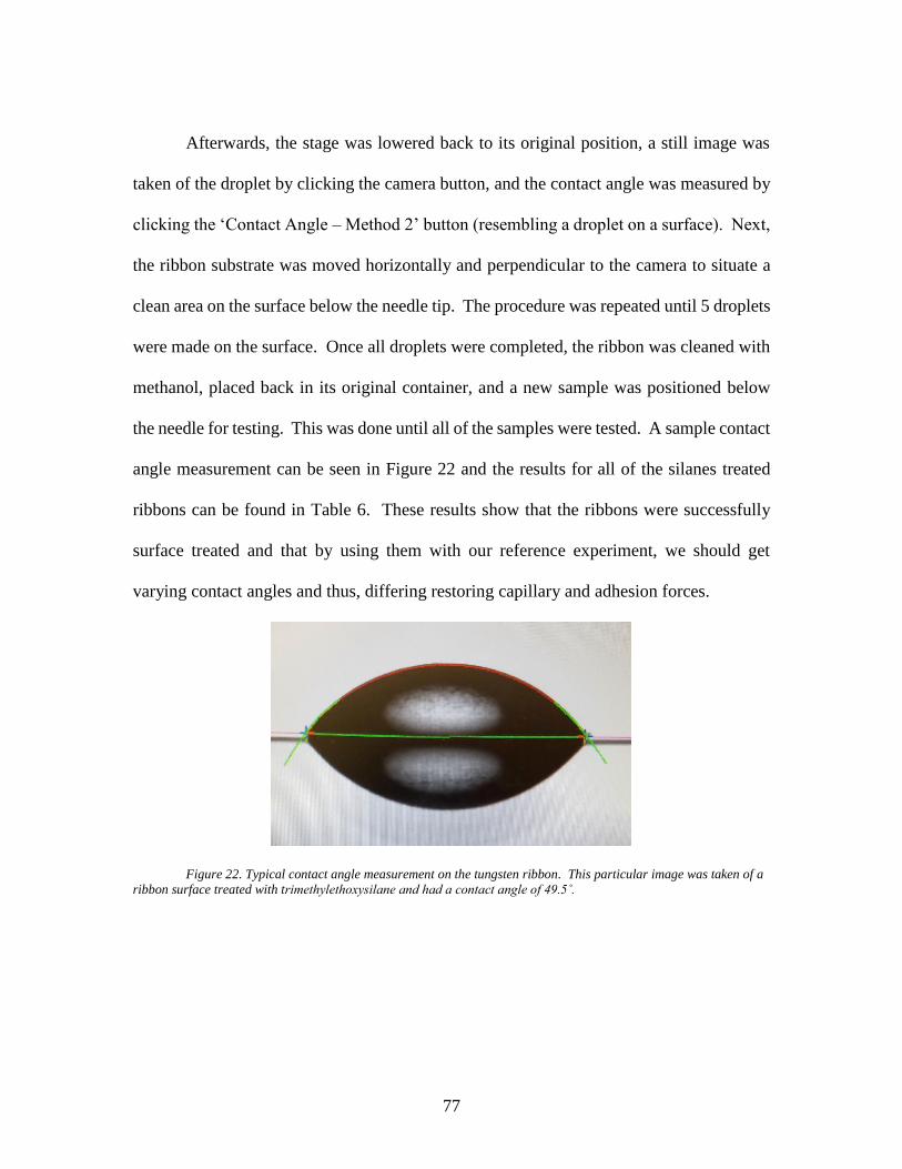
77

Afterwards, the stage was lowered back to its original position, a still image was

taken of the droplet by clicking the camera button, and the contact angle was measured by

clicking the ‘Contact Angle – Method 2’ button (resembling a droplet on a surface). Next,

the ribbon substrate was moved horizontally and perpendicular to the camera to situate a

clean area on the surface below the needle tip. The procedure was repeated until 5 droplets

were made on the surface. Once all droplets were completed, the ribbon was cleaned with

methanol, placed back in its original container, and a new sample was positioned below

the needle for testing. This was done until all of the samples were tested. A sample contact

angle measurement can be seen in Figure 22 and the results for all of the silanes treated

ribbons can be found in Table 6. These results show that the ribbons were successfully

surface treated and that by using them with our reference experiment, we should get

varying contact angles and thus, differing restoring capillary and adhesion forces.

Figure 22. Typical contact angle measurement on the tungsten ribbon. This particular image was taken of a

ribbon surface treated with trimethylethoxysilane and had a contact angle of 49.5˚.

78

Table 6. Contact angle measurements on the surface of treated tungsten wires.

6.1.4 Future of the Project

Experimental videos with this reference experiment have been gathered with

various combinations of tungsten ribbons, surface treatments, and wetting agents

(mentioned in Chapters 6.1.2 and 6.1.3); however, the experimental videos have not been

analyzed with our Mathematica code. This is due to a difference in the capillary forces

between the flat ribbons (compared to the c-shape food canal of the galeae). The capillary

force between the galeae for small distances of separation could be approximated by the

linear equation seen previously [5]; however, due to the flat surfaces of the ribbons, there

is a singularity in the theoretical capillary force profile (goes to infinity as the distance

between the two faces come close together) and as such, we cannot approximate this force

with a linear equation. Due to this non-linearity, we will have to change the model and use

the Euler-Elastica (51), which is the subject of another set of work. Another suggestion

could be to use non-ribbon-like fibers for future testing and as such, our model could

continue to be used. In conclusion, with slight modifications to either our model or sample

shape, the proposed adhesion method can be verified and used for multifunctional

composites to evaluate the fiber-matrix interface along with the adhesion properties.

Surface Treatment Average Contact Angle [˚] Standard Deviation

Untreated 58.5 9.7

3-Methacryloxypropyltrimethoxysilane 81.6 2.4

(3-Glycidyloxypropyl) trimethoxysilane 51.0 3.6

Trimethylethoxysilane 59.3 7.9

79

APPENDICES

80

Appendix A

Table of Collected Data

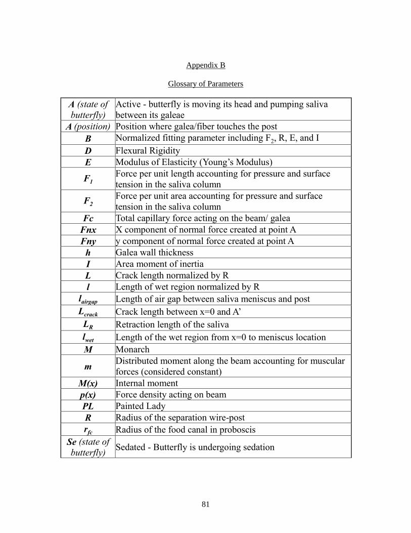
81

Appendix B

Glossary of Parameters

A (state of

butterfly)

Active - butterfly is moving its head and pumping saliva

between its galeae

A (position) Position where galea/fiber touches the post

B Normalized fitting parameter including F2, R, E, and I

D Flexural Rigidity

E Modulus of Elasticity (Young’s Modulus)

F1 Force per unit length accounting for pressure and surface

tension in the saliva column

F2 Force per unit area accounting for pressure and surface

tension in the saliva column

Fc Total capillary force acting on the beam/ galea

Fnx X component of normal force created at point A

Fny y component of normal force created at point A

h Galea wall thickness

I Area moment of inertia

L Crack length normalized by R

l Length of wet region normalized by R

lairgap Length of air gap between saliva meniscus and post

Lcrack Crack length between x=0 and A’

LR Retraction length of the saliva

lwet Length of the wet region from x=0 to meniscus location

M Monarch

m Distributed moment along the beam accounting for muscular

forces (considered constant)

M(x) Internal moment

p(x) Force density acting on beam

PL Painted Lady

R Radius of the separation wire-post

rfc Radius of the food canal in proboscis

Se (state of

butterfly) Sedated - Butterfly is undergoing sedation

82

Sl (state of

butterfly) Sleeping - Butterfly is completely anaesthetized

t Time

V(x) Internal shear force

Vadx Horizontal Adhesion Force - x component of adhesion force

(tangential)

Vady Vertical Adhesion Force - y component of adhesion force

(normal)

X Horizontal position normalized by radius of the post

x Horizontal position along the galeae

Y(X) Deflection normalized by radius of the post

y(x) Deflection of the galea from the x-axis

ycr Measured deflection of the galea at the meniscus position

γ Dimensionless parameter relating F1, F2, and R

θ Angle between x-axis & inwards normal vector of the tangent

line positioned at intersection of galea and post

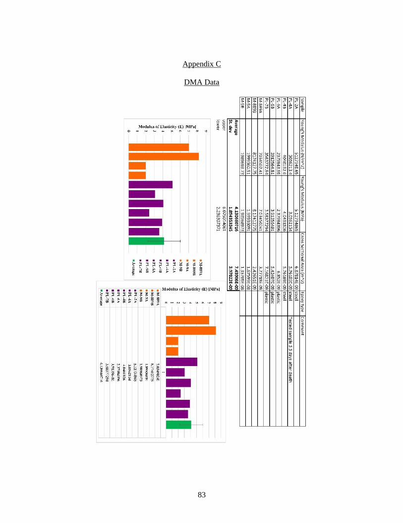
83

Appendix C

DMA Data

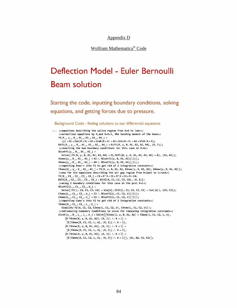
84

Appendix D

Wolfram Mathematica® Code

85

86

87

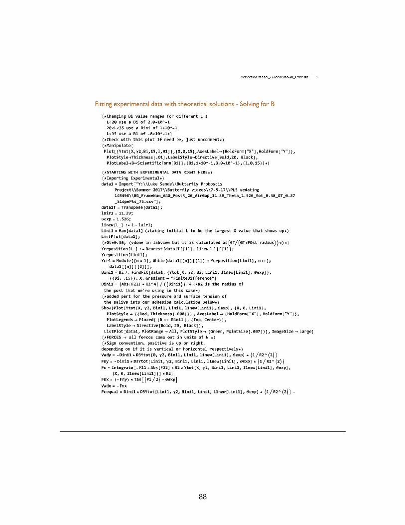
88

89

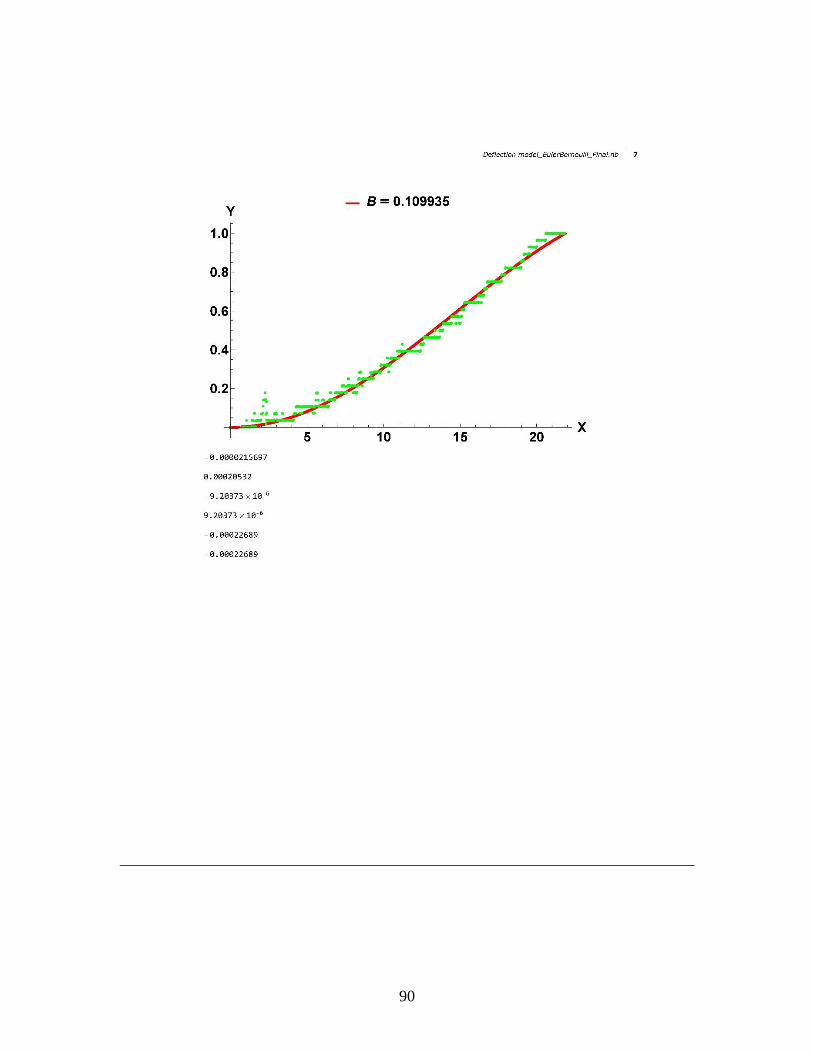
90

91

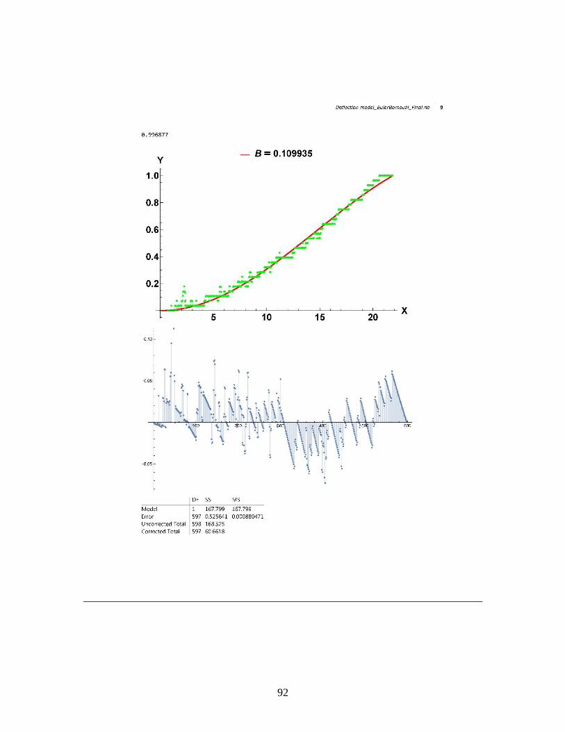
92

93

94

Appendix E

Integration Constants for Solutions to Differential Equations

N11 = 12𝐵𝛾 + 𝐵5𝑙4𝛾 − 4𝐵5𝑙3𝐿𝛾 + 6𝐵5𝑙2𝐿2𝛾 − 4𝐵5𝑙𝐿3𝛾 + 𝐵5𝐿4𝛾 − 12𝐵𝛾Cos[𝐵𝑙] +6𝐵3𝑙2𝛾Cos[𝐵𝑙] − 12𝐵3𝑙𝐿𝛾Cos[𝐵𝑙] + 6𝐵3𝐿2𝛾Cos[𝐵𝑙] + 12𝐵𝑙Cos[𝐵𝑙]Cot[𝜃] −2𝐵3𝑙3Cos[𝐵𝑙]Cot[𝜃] − 12𝐵𝐿Cos[𝐵𝑙]Cot[𝜃] + 6𝐵3𝑙2𝐿Cos[𝐵𝑙]Cot[𝜃] −6𝐵3𝑙𝐿2Cos[𝐵𝑙]Cot[𝜃] + 2𝐵3𝐿3Cos[𝐵𝑙]Cot[𝜃] − 12𝐵2𝑙𝛾Sin[𝐵𝑙] + 12𝐵2𝐿𝛾Sin[𝐵𝑙] −12Cot[𝜃]Sin[𝐵𝑙] + 6𝐵2𝑙2Cot[𝜃]Sin[𝐵𝑙] − 12𝐵2𝑙𝐿Cot[𝜃]Sin[𝐵𝑙] +6𝐵2𝐿2Cot[𝜃]Sin[𝐵𝑙] + 12𝐵Cos[𝐵𝑙]Sin[𝜃] − 6𝐵3𝑙2Cos[𝐵𝑙]Sin[𝜃] +12𝐵3𝑙𝐿Cos[𝐵𝑙]Sin[𝜃] − 6𝐵3𝐿2Cos[𝐵𝑙]Sin[𝜃] + 12𝐵2𝑙Sin[𝐵𝑙]Sin[𝜃] −12𝐵2𝐿Sin[𝐵𝑙]Sin[𝜃] + 𝐵Cosh[𝐵𝑙]((−12 − 12𝐵2(𝑙 − 𝐿)2 + 𝐵4(𝑙 − 𝐿)4)𝛾Cos[𝐵𝑙] −2((6 + 𝐵2(𝑙 − 𝐿)2)(𝑙 − 𝐿)Cot[𝜃] + 4𝐵3(𝑙 − 𝐿)3𝛾Sin[𝐵𝑙] + 3(2 + 𝐵2(𝑙 − 𝐿)2)(−𝛾 +Sin[𝜃]))) + (24𝐵2(𝑙 − 𝐿)𝛾Cos[𝐵𝑙] + 6(2 + 𝐵2(𝑙 − 𝐿)2)Cot[𝜃] + 𝐵((−12 +12𝐵2(𝑙 − 𝐿)2 + 𝐵4(𝑙 − 𝐿)4)𝛾Sin[𝐵𝑙] + 12𝐵(𝑙 − 𝐿)(−𝛾 + Sin[𝜃])))Sinh[𝐵𝑙]

N21 = 6(2𝐵2(𝑙 − 𝐿)𝛾Cos[𝐵𝑙] + 2Cot[𝜃] + 𝐵(−2 + 𝐵2(𝑙 −𝐿)2)𝛾Sin[𝐵𝑙])(−6(2(Cos[𝐵𝑙] − Cosh[𝐵𝑙]) + 𝐵2(𝑙 − 𝐿)2(Cos[𝐵𝑙] + Cosh[𝐵𝑙])) −4𝐵3(𝑙 − 𝐿)3(Sin[𝐵𝑙] − Sinh[𝐵𝑙])) − 6𝐵(−4𝐵3(𝑙 − 𝐿)3𝛾Sin[𝐵𝑙] − 6((2 +𝐵2(𝑙 − 𝐿)2)𝛾Cos[𝐵𝑙] + 2(−𝛾 + (𝑙 − 𝐿)Cot[𝜃] + Sin[𝜃])))

D11 = 2𝐵(12 + 𝐵4𝑙4 − 4𝐵4𝑙3𝐿 + 6𝐵4𝑙2𝐿2 − 4𝐵4𝑙𝐿3 + 𝐵4𝐿4 + Cosh[𝐵𝑙]((−12 +𝐵4(𝑙 − 𝐿)4)Cos[𝐵𝑙] − 4𝐵(3 + 𝐵2(𝑙 − 𝐿)2)(𝑙 − 𝐿)Sin[𝐵𝑙]) − 4𝐵(𝑙 − 𝐿)((−3 +𝐵2(𝑙 − 𝐿)2)Cos[𝐵𝑙] + 3𝐵(−𝑙 + 𝐿)Sin[𝐵𝑙])Sinh[𝐵𝑙])

D21 = −24𝐵(12 + 𝐵4𝑙4 − 4𝐵4𝑙3𝐿 + 6𝐵4𝑙2𝐿2 − 4𝐵4𝑙𝐿3 + 𝐵4𝐿4 + Cosh[𝐵𝑙]((−12 +𝐵4(𝑙 − 𝐿)4)Cos[𝐵𝑙] − 4𝐵(3 + 𝐵2(𝑙 − 𝐿)2)(𝑙 − 𝐿)Sin[𝐵𝑙]) − 4𝐵(𝑙 − 𝐿)((−3 +𝐵2(𝑙 − 𝐿)2)Cos[𝐵𝑙] + 3𝐵(−𝑙 + 𝐿)Sin[𝐵𝑙])Sinh[𝐵𝑙])

N12 = −4𝐵2𝐿(𝐵(−2𝐵𝑙𝛾 + 2𝐵𝐿𝛾 + 2𝐵(𝑙 − 𝐿)𝛾Cos[𝐵𝑙] + 𝐵(𝑙 − 𝐿)2Cot[𝜃] −2𝛾Sin[𝐵𝑙] + 𝐵2𝑙2𝛾Sin[𝐵𝑙] − 2𝐵2𝑙𝐿𝛾Sin[𝐵𝑙] + 𝐵2𝐿2𝛾Sin[𝐵𝑙] + 2𝐵𝑙Sin[𝜃] −2𝐵𝐿Sin[𝜃]) + 𝐵Cosh[𝐵𝑙](2(𝐵(𝑙 − 𝐿)𝛾 + Sin[𝐵𝑙](𝛾 + (−𝑙 + 𝐿)Cot[𝜃] − Sin[𝜃])) +𝐵(𝑙 − 𝐿)Cos[𝐵𝑙]((𝑙 − 𝐿)Cot[𝜃] + 2(−𝛾 + Sin[𝜃]))) − (𝐵(2 + 𝐵2(𝑙 − 𝐿)2)𝛾 −2Cot[𝜃]Sin[𝐵𝑙] − 2𝐵Cos[𝐵𝑙](𝛾 + (−𝑙 + 𝐿)Cot[𝜃] − Sin[𝜃]))Sinh[𝐵𝑙])

N22 = −2𝐵2(𝐵(−2𝐵𝑙𝛾 + 2𝐵𝐿𝛾 + 2𝐵(𝑙 − 𝐿)𝛾Cos[𝐵𝑙] + 𝐵(𝑙 − 𝐿)2Cot[𝜃] −2𝛾Sin[𝐵𝑙] + 𝐵2𝑙2𝛾Sin[𝐵𝑙] − 2𝐵2𝑙𝐿𝛾Sin[𝐵𝑙] + 𝐵2𝐿2𝛾Sin[𝐵𝑙] + 2𝐵𝑙Sin[𝜃] −2𝐵𝐿Sin[𝜃]) + 𝐵Cosh[𝐵𝑙](2(𝐵(𝑙 − 𝐿)𝛾 + Sin[𝐵𝑙](𝛾 + (−𝑙 + 𝐿)Cot[𝜃] − Sin[𝜃])) +𝐵(𝑙 − 𝐿)Cos[𝐵𝑙]((𝑙 − 𝐿)Cot[𝜃] + 2(−𝛾 + Sin[𝜃]))) − (𝐵(2 + 𝐵2(𝑙 − 𝐿)2)𝛾 −2Cot[𝜃]Sin[𝐵𝑙] − 2𝐵Cos[𝐵𝑙](𝛾 + (−𝑙 + 𝐿)Cot[𝜃] − Sin[𝜃]))Sinh[𝐵𝑙])

95

N32 = 2𝐵(𝐵(3(−2 + 𝐵2(𝑙2 − 𝐿2))𝛾Cos[𝐵𝑙] + 𝐵(𝐵(𝑙 − 𝐿)2(2𝑙 + 𝐿)Cot[𝜃] + (𝐵2𝑙3 +2𝐵2𝐿3 − 3𝑙(2 + 𝐵2𝐿2))𝛾Sin[𝐵𝑙] + 3𝐵(𝑙2 − 𝐿2)(−𝛾 + Sin[𝜃]))) + Cosh[𝐵𝑙](3𝐵(2 +

𝐵2(𝑙2 − 𝐿2))𝛾 − 6Sin[𝐵𝑙]((1 + 𝐵2𝑙(𝑙 − 𝐿))Cot[𝜃] + 𝐵2𝑙(−𝛾 + Sin[𝜃])) −1

2𝐵3(𝑙 −

𝐿)Cos[𝐵𝑙]Csc[𝜃](2(−2𝑙2 + 𝑙𝐿 + 𝐿2)Cos[𝜃] − 6(𝑙 + 𝐿)Sin[𝜃](−𝛾 + Sin[𝜃]))) −(𝐵(𝐵(𝐵2𝑙3 + 2𝐵2𝐿3 + 𝑙(6 − 3𝐵2𝐿2))𝛾 + 6Sin[𝐵𝑙](𝛾 + (−2𝑙 + 𝐿)Cot[𝜃] − Sin[𝜃])) +6Cos[𝐵𝑙]((−1 + 𝐵2𝑙(𝑙 − 𝐿))Cot[𝜃] + 𝐵2𝑙(−𝛾 + Sin[𝜃])))Sinh[𝐵𝑙])

D12 = 2(12 + 𝐵4𝑙4 − 4𝐵4𝑙3𝐿 + 6𝐵4𝑙2𝐿2 − 4𝐵4𝑙𝐿3 + 𝐵4𝐿4 + Cosh[𝐵𝑙]((−12 +𝐵4(𝑙 − 𝐿)4)Cos[𝐵𝑙] − 4𝐵(3 + 𝐵2(𝑙 − 𝐿)2)(𝑙 − 𝐿)Sin[𝐵𝑙]) − 4𝐵(𝑙 − 𝐿)((−3 +𝐵2(𝑙 − 𝐿)2)Cos[𝐵𝑙] + 3𝐵(−𝑙 + 𝐿)Sin[𝐵𝑙])Sinh[𝐵𝑙])

96

Appendix F

National Instruments LabVIEW® Code

97

98

99

100

101

102

103

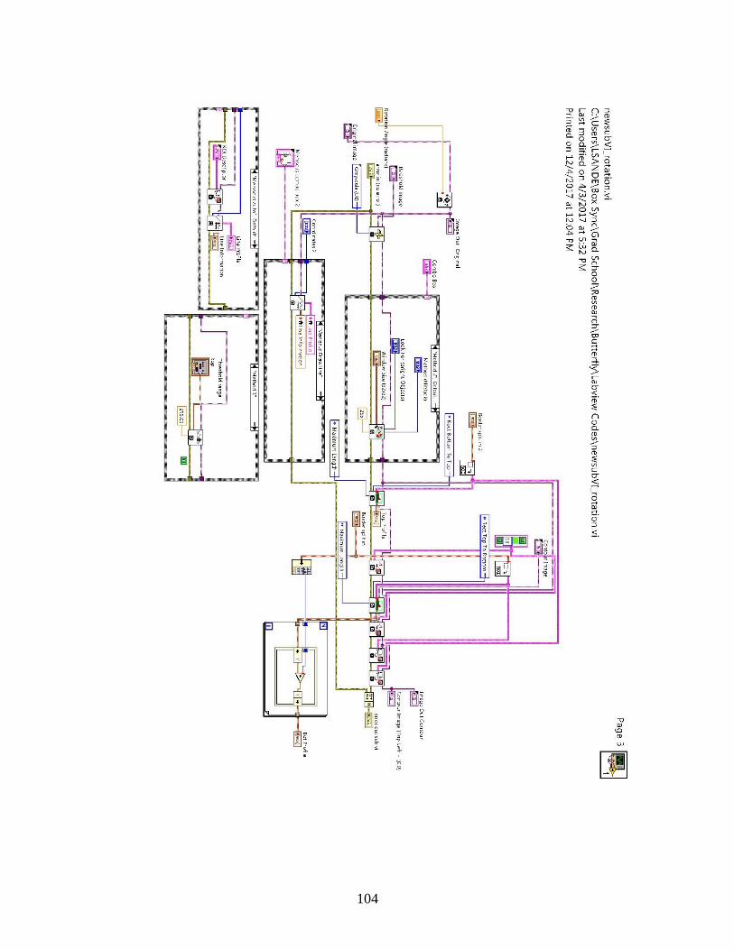
104

105

REFERENCES

1. Kendall K. Molecular Adhesion and Its Applications: The Sticky Universe. New

York: Kluwer Academic/Plenum Publishers; 2001.

2. K.R. S. Contact mechanics and the adhesion of soft solids. Materials Science and

Engineering R. 2002;36:1-45.

3. Kinloch AJ, Williams JG. The mechanics of peel tests. 2002:273-301.

4. Kaelble DH. Theory and Analysis of Peel Adhesion: Mechanisms and Mechanics.

Transactions of the Society of Rheology. 1959;3(1):161-80.

5. Bikerman JJ. Theory of Peeling through a Hookean Solid. Journal of Applied

Physics. 1957;28(12).

6. Crocombe AD, Adams RD. Peel Analysis Using the Finite Element Method. The

Journal of Adhesion. 1981;12(2):127-39.

7. Thouless MD, Jensen HM. Elastic Fracture Mechanics of the Peel-Test Geometry.

The Journal of Adhesion. 1992;38(3-4):185-97.

8. Gibson RF. A review of recent research on mechanics of multifunctional composite

materials and structures. Composite Structures. 2010;92(12):2793-810.

9. Zhandarov S. Characterization of fiber/matrix interface strength: applicability of

different tests, approaches and parameters. Compos Sci Technol. 2005;65(1):149-60.

10. Hoecker F, Karger-Kocsis J. Effects of the interface on the mechanical response of

CF/EP microcomposites and macrocomposites. Composites. 1994;25(7):729-38.

11. Hoecker F, Friedrich K, Blumberg H, Karger-Koscis J. Effects of fiber/matrix

adhesion on off-axis mechanical response in carbon-fiber/epoxy-resin componsites.

Compos Sci Technol. 1995;54:317-27.

12. López-Buendía AM, Romero-Sánchez MD, Climent V, Guillem C. Surface treated

polypropylene (PP) fibres for reinforced concrete. Cement and Concrete Research.

2013;54:29-35.

13. Chandra R, Singh SP, Gubta K. Damping studies in fiber-reinforced composites -

a review. Composite Structures. 1999;46:41-51.

14. Lawcock GD, Ye L, Mai YW, Sun CT. Effects of fiber/matrix adhesion on carbon-

fiber-reinforced metal laminates -- II. Impact behaviour. Compos Sci Technol.

1997;57:1621-8.

15. Effect of High Modulus Polyethylene Fibre Surface Treatment on Epoxy Resin

Composite Impact Properties.

16. Sun L, Gibson RF, Gordaninejad F, Suhr J. Energy absorption capability of

nanocomposites: A review. Compos Sci Technol. 2009;69(14):2392-409.

17. Tehrani M, Safdari M, Boroujeni AY, Razavi Z, Case SW, Dahmen K, et al. Hybrid

carbon fiber/carbon nanotube composites for structural damping applications.

Nanotechnology. 2013;24(15):155704.

18. Rajoria H, Jalili N. Passive vibration damping enhancement using carbon nanotube-

epoxy reinforced composites. Compos Sci Technol. 2005;65(14):2079-93.

19. Gibson RF, Chen Y, Zhao H. Improvement of Vibration Damping Capacity and

Fracture Toughness in Composite Laminates by the Use of Polymeric Interleaves. Journal

of Engineering Materials and Technology. 2001;123(3):309.

106

20. Gottardo L, Hufenus R, Dressler M, Heuberger M. Design and development of

liquid filled polymeric fibers with flexure rate viscoelastic properties. Aip Conf Proc.

2014;1593:60-3.

21. Khan SU, Li CY, Siddiqui NA, Kim J-K. Vibration damping characteristics of

carbon fiber-reinforced composites containing multi-walled carbon nanotubes. Compos

Sci Technol. 2011;71(12):1486-94.

22. Rao V, Herrera-Franco P, Ozzello AD, Drzal LT. A direct comparison of the

fragmentation test and the microbond pull-out test for determining the interfacial shear

strength. J Adhes. 1991;34:65-77.

23. Hassoune-Rhabbour B, Poussines L, Nassiet V. Development of an Adhesion Test

for Characterizing the Interface Fiber/Polymer Matrix. Key Engineering Materials.

2012;498:210-8.

24. Ostrowicki GT, Sitaraman SK. Magnetically actuated peel test for thin films. Thin

Solid Films. 2012;520(11):3987-93.

25. Vanwalleghem J, De Baere I, Huysman S, Lapeire L, Verbeken K, Nila A, et al.

Effective use of transient vibration damping results for non-destructive measurements of

fibre-matrix adhesion of fibre-reinforced flax and carbon composites. Polymer Testing.

2016;55:269-77.

26. Wu HF, Gu W, Lu G-Q, Kampe SL. Non-destructive characterization of fibre–

matrix adhesion in composites by vibration damping. Journal of Materials Science.

1997;32(7):1795-8.

27. M. N, Chen EJH. Review of Methods for Characterization of Interfacial Fiber-

Matrix Interactions. Polymer Composites. 1988;9(4):245-51.

28. Eitner U, Rendler LC. The Mechanical Theory behind the Peel Test. Energy

Procedia. 2014;55:331-5.

29. Brown HR, Yang ACM. The use of peel tests to examine the self adhesion of

polyimide films. Journal of Adhesion Science and Technology. 1991;6(3):333-46.

30. Jang J, Sung M, Han S, Yu W-R. Prediction of delamination of steel-polymer

composites using cohesive zone model and peeling tests. Composite Structures.

2017;160:118-27.

31. Kinloch AJ, Lau CC, Williams JG. The peeling of flexible laminates. International

Journal of Fracture. 1994;66:45-70.

32. Zhang Y, Hazelton DW, Knoll AR, Duval JM, Brownsey P, Repnoy S, et al.

Adhesion strength study of IBAD–MOCVD-based 2G HTS wire using a peel test. Physica

C: Superconductivity. 2012;473:41-7.

33. Yang QD, Thouless MD, Ward SM. Analysis of the Symmetrical 90°-peel Test

with Extensive Plastic Deformation. The Journal of Adhesion. 2006;72(2):115-32.

34. Krenn HW. Feeding mechanisms of adult Lepidoptera: structure, function, and

evolution of the mouthparts. Annu Rev Entomol. 2010;55:307-27.

35. Lehnert MS, Monaenkova D, Andrukh T, Beard CE, Adler PH, Kornev KG.

Hydrophobic-hydrophilic dichotomy of the butterfly proboscis. J R Soc Interface.

2013;10(85):20130336.

36. Krenn HW. Proboscis Morphology and Food Preferences in Nymphalid Butterflies

(Lepidoptera: Nymphalidae). The Zoological Society of London. 2001;254:17-26.

107

37. Tsai CC, Mikes P, Andrukh T, White E, Monaenkova D, Burtovyy O, et al.

Nanoporous artificial proboscis for probing minute amount of liquids. Nanoscale.

2011;3(11):4685-95.

38. Monaenkova D, Lehnert MS, Andrukh T, Beard CE, Rubin B, Tokarev A, et al.

Butterfly proboscis: combining a drinking straw with a nanosponge facilitated

diversification of feeding habits. J R Soc Interface. 2012;9(69):720-6.

39. Kingsolver JG, Daniel TL. Mechanics of Food Handling by Fluid-Feeding Insects.

In: Chapman RF, de Boer G, editors. Regulatory Mechanisms in Insect Feeding. Boston,

MA: Springer US; 1995. p. 32-73.

40. Krenn HW. Proboscis assembly in butterflies (Lepidoptera) - a once in a lifetime

sequence of events. Eur J Entomol. 1996(94):495-501.

41. Hepburn HR. Proboscis Extension and Recoil in Lepidoptera. Journal of Insect

Physiology. 1970;17:637-56.

42. Keis K, Kornev KG, Kamath YK, Neimark AV. Towards Fiber-Based Micro- and

Nanofluidics. 2007. In: Nanoengineered Nanofibrous Materials [Internet].

43. Kornev KG, Adler PH. The Butterfly Proboscis as a Fiber-Based, Self-Cleaning

Microfluidic System. SPIE Newsroom. 2014;4:6934.

44. Pometto S. Repair of the proboscis of brush-footed butterflies (lepidoptera:

Nymphalidae). Tiger Prints: Clemson University; 2014.

45. Krenn HW, Kristensen NP. Evolution of proboscis musculature in lepidoptera. Eur

J Entomol. 2004;101(4):565-75.

46. Liu J, Gong Y, Cao G. Chemical mediated elasto-capillarity of elastic sheets. Soft

Matter. 2017.

47. Roman B, Bico J. Elasto-capillarity: deforming an elastic structure with a liquid

droplet. J Phys Condens Matter. 2010;22(49):493101.

48. Bico J, Roman B, Moulin L, Boudaoud A. Elastocapillary coalescence in wet hair.

Nature Brief Communications. 2004;432:690.

49. Monaenkova D, Andrukh T, Kornev KG. Bernoulli catenary and elasto-capillary

effect in partially wet fibrous materials. Textile Research Journal. 2013;83(13):1386-97.

50. Hartog JPD. Advanced Strength of Materials: Dover Publications; 1987.

51. Landau LD, Lifshitz EM. Theory of Elasticity. 3 ed: Reed Educational and

Professional Publishing Ltd.; 1986.

52. Timoshenko S, Goodier JN. Theory of Elasticity. 2 ed. United States: McGraw-Hill

Book Company, Inc.; 1934. 35 p.

53. Kreyszig E. Advanced Engineering Mathematics. 10 ed: Wiley; 2011. 1280 p.

54. Obreimoff JW. The Splitting Strength of Mica. J R Soc Interface.

1930;127(805):290-7.

55. Pometto SF. Saliva Collection and Quantification from Adult Butterflies

(Lepidoptera). Entomological News. 2015;124(5):305-9.

56. Capinera JL. Encyclopedia of Entomology. 2 ed: Springer Netherlands; 2008. 4346

p.

57. Scudder SH. The Butterflies of the Eastern United States and Canada. 1889;1.

58. Nicolas G. Immediate and Latent Effects of Carbon Dioxide on Insects. Annu Rev

Entomol. 1989;34:97-116.

108

59. Quan C, Hu Z, Qian K, Li G, Xie H, Asundi AK, et al. Measurement of Young's

modulus and Poisson's ratio of human hair using optical techniques. 2009;7522:75222Q.