€¦ · MAT Serie A: CONFERENCIAS, SEMINARIOS Y TRABAJOS DE MATEMATICA ISSN: 1515-4904 Propiedad de ACES DIRECTOR D. A. TARZIA Departamento de …

C o n f e r e n c i a s , s e m i n a r i o s y t r a b a j o s d e M a t e m a t i c a

I S S N : 1 5 1 5 - 4 9 0 4

Terceras Jornadas

sobre Ecuaciones

Diferenciales,

Optimizacion y

A nalisis Numerico

Maria C. Maciel

Domingo A. Tarzia (EGIS.)

MAT

Serie A: CONFERENCIAS, SEMINARIOS Y TRABAJOS DE MATEMATICA ISSN: 1515-4904

Propiedad de ACES DIRECTOR

D. A. TARZIA Departamento de Matemática – CONICET, FCE-UA, Paraguay 1950, S2000FZF ROSARIO, ARGENTINA.

[email protected] COMITE EDITORIAL Y CIENTIFICO

L. A. CAFFARELLI Department of Mathematics, Univ. of Texas at Austin, RLM 8100 Austin, TEXAS 78712, USA.

[email protected] R. DURAN Departamento de Matemática, FCEyN, Univ. de Buenos Aires, Ciudad Universitaria, Pab. 1, 1428 BUENOS AIRES, ARGENTINA. [email protected] A. FASANO Dipartimento di Matematica “U. Dini”, Univ. di Firenze,

Viale Morgagni 67/A, 50134 FIRENZE, ITALIA. [email protected]

J.L. MENALDI Department of Mathematics, Wayne State University, Detroit, MI 48202, USA.

[email protected] M. PRIMICERIO Dipartimento di Matematica “U. Dini”, Univ. di Firenze,

Viale Morgagni 67/A, 50134 FIRENZE, ITALIA. [email protected]

C.V. TURNER FAMAF, Univ. Nac. de Córdoba, Ciudad Universitaria, 5000 CORDOBA, ARGENTINA. [email protected]

R. WEDER Instituto de Investigaciones en Matemáticas Aplicadas y en Sistemas, Univ. Nac. Autónoma de México (UNAM) Apartado Postal 20-726, MEXICO, DF 010000.

[email protected] N. WOLANSKI Departamento de Matemática, FCEyN, Univ. de Buenos Aires, Ciudad Universitaria, Pab. 1, 1428 BUENOS AIRES, ARGENTINA. [email protected] SECRETARIA DE REDACCION

G. GARGUICHEVICH Departamento de Matemática, FCE-UA, Paraguay 1950, S2000FZF ROSARIO, ARGENTINA.

[email protected] MAT es una publicación del Departamento de Matemática de la Facultad de Ciencias Empresariales de la Universidad Austral (FCE-UA) cuyo objetivo es contribuir a la difusión de conocimientos y resultados matemáticos. Se compone de dos series: • Serie A: CONFERENCIAS, SEMINARIOS Y TRABAJOS DE MATEMATICA. • Serie B: CURSOS Y SEMINARIOS PARA EDUCACION MATEMATICA. La Serie A contiene trabajos originales de investigación y/o recapitulación que presenten una exposición interesante y actualizada de algunos aspectos de la Matemática, además de cursos, conferencias, seminarios y congresos realizados en el Depto. de Matemática. El Director, los miembros del Comité Editorial y Científico y/o los árbitros que ellos designen serán los encargados de dictaminar sobre los merecimientos de los artículos que se publiquen. La Serie B se compone de cursos especialmente diseñados para profesores de Matemática de cada uno de los niveles de educación: E.G.B., Polimodal, Terciaria y Universitaria. Las publicaciones podrán ser consultadas en: www.austral.edu.ar/MAT

ISSN 1515-4904

MAT

SERIE A: CONFERENCIAS, SEMINARIOS Y TRABAJOS DE MATEMÁTICA

No. 14

TERCERAS JORNADAS SOBRE ECUACIONES DIFERENCIALES, OPTIMIZACIÓN Y ANÁLISIS NUMÉRICO

Maria Cristina Maciel - Domingo Alberto Tarzia (Eds.)

INDICE Tatiana I. Gibelli – María C. Maciel, “Large-scale algorithms for minimizing a linear function with a strictly convex quadratic constraint”, 1-12. María C. Maciel – Elvio A. Pilotta – Graciela N. Sottosanto, “Thickness optimization of an elastic beam”, 13-23. María F. Natale – Eduardo A. Santillan Marcus – Domingo A. Tarzia, “Determinación de dos coeficientes térmicos a través de un problema de desublimación con acoplamiento de temperatura y humedad”, 25-30. Rubén D. Spies – Karina G. Temperini, “Sobre la no convergencia del método de mínimos cuadrados en dimension infinita”, 31-34. Juan C. Reginato – Domingo A. Tarzia, “An alternative method to compute Michaelis-Menten parameters from nutrient uptake data”, 35-40.

Rosario, Marzo 2007

Las Terceras Jornadas sobre Ecuaciones Diferenciales, Optimización y Análisis Numérico tuvieron lugar en el Departamento de Matemática de la Universidad Nacional del Sur, en la ciudad de Bahía Blanca, del 9 al 10 de Marzo de 2006. Fue realizado con el apoyo del Proyecto de Investigación Plurianual “Partial Differential Equations and Numerical Optimization with Applications” subsidiado por la Fundación Antorchas e integrado por los siguientes subproyectos:

• “Free Boundary Problems for the Heat-Diffusion Equation” (UA-UNR-UNRC-UNSa); • “Inverse and Control Problems in the Mathematical Modeling of Phase Transitions in Shape

Memory Alloys” (UNL); • “Geophysical Scale Stratified Flows and Hydraulic Jumps” (UNC-UBA-UNLPa); • “Optimization Applied to Mechanical Engineering Problems” (UNS-UNC-UNCo).

El Comité Organizador estuvo compuesto por: M.C. Maciel (Bahía Blanca, Coordinadora), R.D. Spies (Santa Fe), D. A. Tarzia, (Rosario); C.V. Turner (Córdoba). La Secretaría Local estuvo compuesta por: Gabriela Eberle, Tatiana Gibelli y Adriana Verdiell (Coordinadora). Las Jornadas estuvieron dirigidas a graduados, profesionales y estudiantes de Matemática, Física, Química, Ingeniería y ramas afines, con conocimientos básicos sobre ecuaciones diferenciales, análisis numérico y optimización. En MAT – Serie A, # 14 (2007) se publican cinco de las conferencias y comunicaciones presentadas. Los manuscritos fueron recibidos y aceptados en marzo de 2007.

CONFERENCIAS Y COMUNICACIONES DE LAS TERCERAS JORNADAS SOBRE ECUACIONES DIFERENCIALES, OPTIMIZACIÓN Y ANÁLISIS NUMÉRICO

Jueves 9 de marzo de 2006

• Gabriela Eberle (Bahía Blanca), "Método de Newton en espacios matriciales". • Adriana Verdiell (Bahía Blanca), "Manejo de áreas naturales: alcances y limitaciones de un modelo

matemático". • María Cristina Maciel (Bahía Blanca), "Aplicación de la condición PLD al problema de

optimización multiobjetivo". • Olga Emilia Mandrini (Neuquén), "Sobre la resolución numérica de un problema de optimización de

formas". • Tatiana Gibelli (Bahía Blanca), "Un algoritmo para minimización de función lineal con restricciones

cuadráticas convexas". • María Cristina Sanziel (Rosario), "Optimización del flujo total de calor en un problema con

restricciones de temperatura, a través de un problema de Cauchy para la ecuación de Laplace". • Mariela C. Olguin (Rosario), "Comportamiento monótono de la temperatura y la frontera libre de

una sustancia, respecto de la variación de sus coeficientes térmicos". • Domingo A. Tarzia (Rosario), "La ecuación del calor no-clásica. Solución explícita para un

problema de Stefan con dato de temperatura en el borde fijo". • Eduardo A. Santillan Marcus (Rosario), "Un problema de desublimación en un medio poroso

húmedo". Viernes 10 de marzo de 2006:

Rubén Spies (Santa Fe), "Sobre un modelo termoelástico para los movimientos de las antenas del Telescopio espacial James Webb".

Karina Temperini (Santa Fe), "Divergencia con velocidad arbitraria del método de mínimos cuadrados en problemas inversos mal condicionados".

Jorge L. Blengino (Río Cuarto), "Toma de agua por raíces de cultivos. Algunos resultados numéricos".

Juan C. Reginato (Río Cuarto), "Interaccciones en la toma de nutrientes. Uso de cinéticas competitivas en un modelo de frontera móvil".

Marcos Gaudiano (Córdoba), “Condición convectiva en la difusión de un solvente en un polímero vidrioso”.

MAT-Serie A, 14(2007), 1-12 1

LARGE-SCALE ALGORITHMS FOR MINIMIZING A LINEAR FUNCTIONWITH A STRICTLY CONVEX QUADRATIC CONSTRAINT1

T.I. GIBELLI 2 and M.C MACIEL 3

Departamento de Matematica, Universidad Nacional del SurAv. Alem 1253, 8000 Bahıa Blanca, Argentina.

Abstract

The problem of minimizing a linear function subject to convex quadratic constraints appearsin many topological optimization problems such as truss and free material optimization.Usually this kind of problems is solved using interior point methods. In this work, theproblem with only one constraint is considered. The solution of the problem is analyzedwhen the constraint matrix is symmetric and positive definite. A simple iterative algorithmis proposed. It is essentially based on the steepest descent direction and the geometricproperties of the problem. In this method an iteration goes to the boundary in the negativegradient direction and then it finds the center of the region determined by the intersectionof the level hyperplane and the feasible set. The convergence of this algorithm is analyzed.Also, an improved version of the algorithm is established. It comes from the observationthat centers are in the same line, so only one center-finding operation is needed. Becauseof its simplicity, these algorithms are appropriate for very large scale problems. Numericalresults are presented.

Key words: Quadratic Constraints, Topological Optimization.AMS Subject Classification: 49M40, 49N10, 90C25, 90C30.

1 Introduction

Some topologic optimization problems, like truss and free material optimization, can be estab-lished as a constrained optimization problem as follows

mins.t.

cTx12xTAix ≤ bi, i = 1, ..., m,

(1)

where c ∈ Rn, Ai ∈ Rn×n are symmetric positive semidefinite matrices, and bi ∈ R for alli = 1, ..., m [3].

This kind of problems belongs to the more general class of convex optimization problems:

mins.t.

f(x)

gi(x) ≤ 0, i = 1, ..., m,(2)

where f, gi : Rn → R are twice continuously differentiable convex functions, the set of optimalsolutions is a nonempty and compact set and there exists a point x such as gi(x) < 0 for alli = 1, ..., m.

Many numerical methods solve the problem under some additional assumptions. The inte-rior point methods are perhaps the most popular [1, 4, 6, 10]. They are used to transform a

1This work has been partially supported by Universidad Nacional del Sur, Project 24/069 and FundacionAntorchas, Project 13900-4.

[email protected]. [email protected]. Fax: 54-291-4595163.

Gibelli–Maciel, Strictly convex quadratic constrained linear problem, MAT-Serie A, 14(2007), 1-12 2

constrained problem to a sequence of unconstrained problems, which are solved via well knownalgorithms, for instance the Newton method. Ben-Tal and Zibulesvsky [2] have developed anefficient method for large scale convex problems which are very common in topological design.The algorithm combines ideas of penalty and barrier methods with the Augmented Lagrangianmethod.

In this work, the problem (1) is analyzed with only one quadratic constraint, and the matrixis symmetric and positive definite. First, the existence of solution and its exact expression isstudied. Then, according to the geometric characteristics of the problem an iterative algorithmis proposed to find the solution. The convergence of this algorithm is analyzed. Finally, animproved version of the algorithm is presented and some numerical results are shown to illustratethe behavior of the algorithms.

2 The problem

We consider the optimization problem

mins.t.

f(x) = cTx

12xTAx − dTx ≤ b,

(3)

where c ∈ Rn, c 6= 0, d ∈ Rn, A ∈ Rn×n is a symmetric positive definite matrix and b ∈ R, b > 0.The problem (3) can be transformed into the following one

mins.t.

cTx

12xT Ax ≤ b,

(4)

via a simple substitution. Such a substitution consists of translating the center of the quadratic12xTAx − dTx = b to the origin.

The proposed algorithm is based on the geometric properties of the last problem. We statesome of them.

Lemma 2.1 The problem (4) has a unique solution x∗ and it satisfies that Ax∗ and c are paralleldirections.

Proof: It is straightforward.

........

............................................

......................

..........................

..................................

................................................

............................................................................................................................................................................................................................................................................................................................................................................................................................................................................................................................................................................................................................................................................................................................................................................................................................................................................

...............................................

..................................

.............................................................................................................

...............................................................................................................................................................

v = −c

•xmin

•xmaxxTAx = 2b

...................................

...................................

...................................

...................................

...................................

...................................

...................................

...................................

...................................

......

cT x = cTxmin

...................................

...................................

...................................

...................................

...................................

...................................

...................................

...................................

...................................

...................................

...................................

..................................

...................................

...................................

...................................

...................................

..........................

..................................

...................................

...................................

...................................

...................................

...................................

...................................

...................................

...................................

...................................

...................................

...................................

...................................

...................................

...................................

...................................

..........................

...................................

...................................

...................................

...................................

...................................

...................................

...................................

...................................

...................................

......

cTx = cTxmax

Figure 1: The geometric properties of the problem

Lemma 2.2 The problem (4), where c ∈ Rn, c 6= 0, A = In, and b is a positive real number,

has a unique solution x∗ = −

√2b

cT cc.

Proof: It is straightforward.


Theorem 2.1 The problem (4) has a unique solution, x∗ = −

√2b

cT A−1cA−1c.

Proof: It follows from Lemma 2.1.

3 The algorithm

The exact solution of problem (4) requires the computation of the inverse matrix of A. Itis well known that this computation is not convenient because of the numerical errors and thearithmetic cost. Then, we propose an iterative method which does not require the inverse matrixof A and takes into account the geometric properties of the problem described above.

The main idea is to find alternatively an interior point and a border point following thesteepest descent direction of the objective function until the minimizer is reached. The algorithmstarts with an interior point. Without of generality, let us take y1 = 0.

Figure 2 shows the sequence of interior and border points generated by this algorithm.

........

............................................

.......................

..........................

...................................

................................................

..........................................................................................................................................................................................................................................................................................................................................................................................................................................................................................................................................................................................................................................................................................................................................................................................................................................................................

...............................................

..................................

....................................................................................................• y1

...............................................................................................................................................................................................................................

x(t) = y1 − tc

• y2................................................................................................................

x(t) = y2 − tc

• x1

..................................

...................................

...................................

...................................

...................................

...................................

...................................

...................................

...................................

...................................

...................................

...................................

...................................

...................................

...................................

.................................

cTx = cT x1

•x2

...................................

...................................

...................................

...................................

...................................

...................................

...................................

...................................

...................................

...................................

...................................

...................................

...................................

...................................

...................................

................................

cT x = cTx2

xT Ax = 2b

Figure 2: The behavior of the iterative method

Algorithm 1:Given: c ∈ Rn, c 6= 0, A ∈ Rn×n symmetric and positive definite matrix and b ∈ R, b > 0.For k = 1, 2, .... “until convergence” repeat

Step 1:

– If k = 1, y1 = 0.

– If k > 1, find an interior point yk as the center of the resulting intersection betweenthe level hyperplane cTx = cTxk−1 and the constraint.

Step 2: Find a border point xk as the intersection between the halfline passing throughyk in the direction v = −c and the constraint.

Now let us describe in details Step 1 and 2.

• Step 1: (k > 1) Since c 6= 0, there exists at least an index i such that ci 6= 0. Iffk−1 = cTxk−1, then from the hyperplane cTx = fk−1 it is possible to obtain the component

xi =1ci

fk−1 −

n∑

j 6=i, j=1

cj xj

.


Then,

x1...

xi−1

xi

xi+1...

xn

=

1 0 . . . . . . 0 00 1 . . . . . . 0 0...

.... . .

......

...

−c1

ci. . . −

ci−1

ci−

ci+1

ci. . . −

cn

ci...

......

. . ....

...0 0 . . . . . . 1 00 0 . . . . . . 0 1

x1...

xi−1

xi+1...

xn

+fk−1

ci

0...010...0

.

Let

– P ∈ Rn×(n−1) be the matrix obtained from the identity In−1 ∈ R(n−1)×(n−1) addingthe zero vector as the i-th row . Clearly PPT = In and PT P = In−1.

– e =ei

ci, where eT

i = (0, 0, ..., 1place i

, ..., 0, 0)∈ Rn.

So x = Bx + fk−1e where B = (In − ecT )P ∈ Rn×(n−1) and x = PT x ∈ Rn−1. Theintersection between the hyperplane x = Bx + fk−1e with the constraint 1

2xT Ax = b is

12(Bx + fk−1e)T A(Bx + fk−1e) = b

12xT BT ABx + fk−1e

T ABx +12f2k−1e

TAe = b

12xT Ax − dk

Tx = bk,

where A = BT AB, dk = −fk−1BT Ae y bk = b− 1

2f2k−1e

T Ae.

The center yk of 12 xT Ax − dk

Tx = bk can be obtained by solving the linear system Ax =

dk or equivalently by obtaining the minimizer of the quadratic function 12 xT Ax − dk

Tx.

Clearly, that point can be obtained via any minimization algorithm.

Finally, yk = Byk + fk−1e.

• Step 2: The point xk is obtained as the intersection between the halfline x(t) = yk − tc,t > 0, and the quadratic constraint xTAx = 2b. Then,

(yk − tc)TA(yk − tc) = 2b

yTk Ayk − 2tcT Ayk + t2cTAc = 2b

(cTAc)t2 + 2(−cTAyk)t + (yTk Ayk − 2b) = 0

tk =cT Ayk +

√(cTAyk)2 − (cTAc)(yT

k Ayk − 2b)

cTAcxk = yk − tkc.

• Stopping criterion: the termination rules to stop the algorithm are the following:

– if the closeness between interior and border points is less or equal to a given tolerance‖yk − xk‖

‖xk‖≤ tolerance, or


– if the closeness between iterates,‖xk−1 − xk‖

‖xk‖≤ tolerance.

After these considerations, Algorithm 1 can be written as

Algorithm 1:

Given: c 6= 0 ∈ Rn, A ∈ Rn×n symmetric and positive definite and b ∈ R, b > 0.

Compute: B, e, A = BT AB and v = BT Ae.

For k = 1, 2, .... “until convergence” repeat

Step 1:• If k = 1, y1 = 0.• If k > 1,

∗ compute: fk−1 = cTxk−1 and dk = −fk−1v.

∗ yk = argmin12xT Ax − dk

Tx.

∗ yk = Byk + fk−1e.

Step 2:

• tk =cTAyk +

√(cTAyk)2 − (cTAc)(yT

k Ayk − 2b)

cTAc.

• xk = yk − tkc.

4 Convergence of the algorithm

In this section the behavior of the sequences of interior and border points, yk and xk,generated by the algorithm is analyzed. It will be show that both sequences converge to thesolution of the problem (4).

Lemma 4.1 Let fk, with fk = cTxk and yk, the sequences generated by Algorithm 1, and

x∗ = −

√2b

cTA−1cA−1c the solution of problem (4), then

i) fk is a negative decreasing sequence.

0 > f1 > f2 > ... > fk−1 > fk > fk+1 > ...

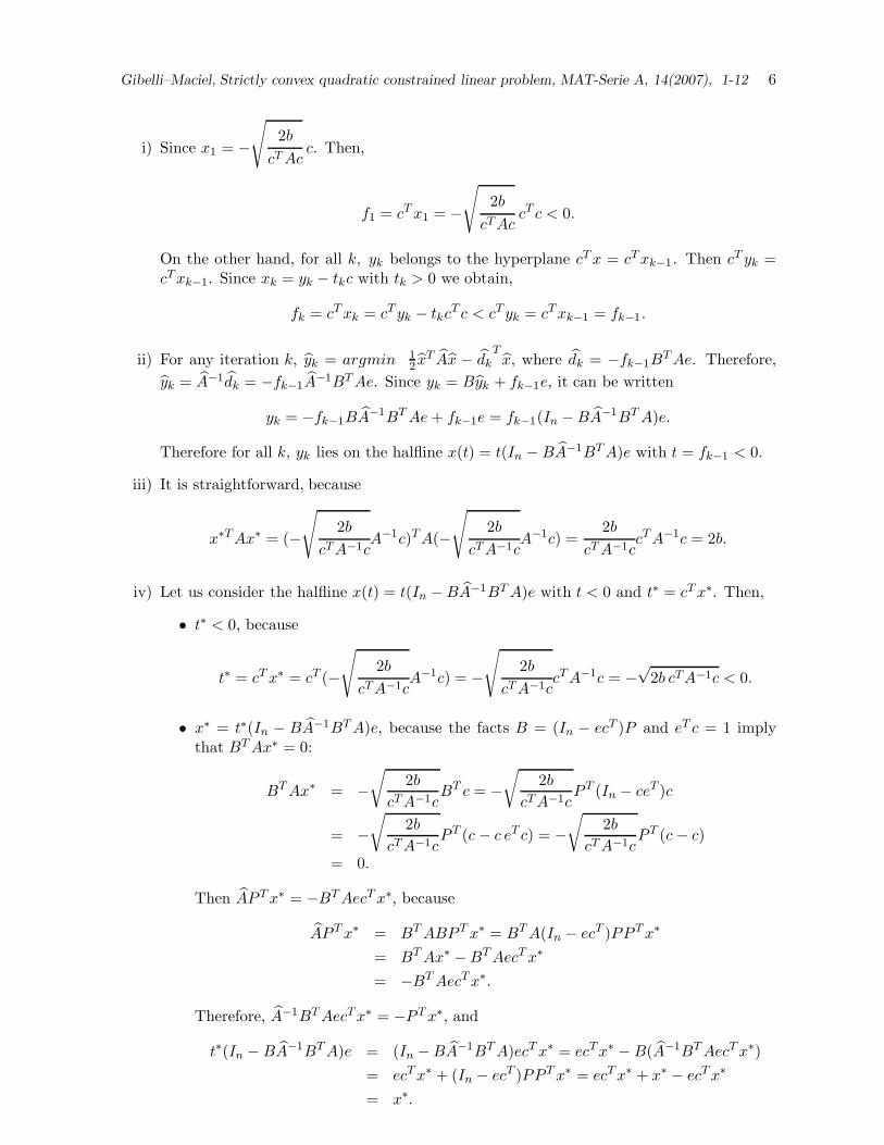
ii) Each term yk belongs to the halfline x(t) = t(In − BA−1BT A)e, t < 0.

iii) x∗TAx∗ = 2b.

iv) x∗ is located to the line x(t) = t(In − BA−1BT A)e, t < 0.

Proof:


i) Since x1 = −

√2b

cT Acc. Then,

f1 = cT x1 = −

√2b

cTAccT c < 0.

On the other hand, for all k, yk belongs to the hyperplane cT x = cTxk−1. Then cT yk =cTxk−1. Since xk = yk − tkc with tk > 0 we obtain,

fk = cTxk = cTyk − tkcT c < cTyk = cTxk−1 = fk−1.

ii) For any iteration k, yk = argmin 12 xT Ax − dk

Tx, where dk = −fk−1B

T Ae. Therefore,yk = A−1dk = −fk−1A

−1BT Ae. Since yk = Byk + fk−1e, it can be written

yk = −fk−1BA−1BT Ae + fk−1e = fk−1(In − BA−1BT A)e.

Therefore for all k, yk lies on the halfline x(t) = t(In − BA−1BT A)e with t = fk−1 < 0.

iii) It is straightforward, because

x∗TAx∗ = (−

√2b

cTA−1cA−1c)TA(−

√2b

cTA−1cA−1c) =

2b

cT A−1ccTA−1c = 2b.

iv) Let us consider the halfline x(t) = t(In − BA−1BT A)e with t < 0 and t∗ = cT x∗. Then,

• t∗ < 0, because

t∗ = cT x∗ = cT (−

√2b

cTA−1cA−1c) = −

√2b

cTA−1ccTA−1c = −

√2b cTA−1c < 0.

• x∗ = t∗(In − BA−1BT A)e, because the facts B = (In − ecT )P and eT c = 1 implythat BT Ax∗ = 0:

BT Ax∗ = −√

2b

cTA−1cBT c = −

√2b

cTA−1cPT (In − ceT )c

= −√

2b

cTA−1cPT (c − c eT c) = −

√2b

cTA−1cPT (c − c)

= 0.

Then APT x∗ = −BT AecT x∗, because

APT x∗ = BT ABPT x∗ = BT A(In − ecT )PPT x∗

= BT Ax∗ − BT AecT x∗

= −BT AecTx∗.

Therefore, A−1BT AecTx∗ = −PT x∗, and

t∗(In − BA−1BT A)e = (In − BA−1BT A)ecT x∗ = ecTx∗ − B(A−1BT AecT x∗)= ecTx∗ + (In − ecT )PPT x∗ = ecTx∗ + x∗ − ecTx∗

= x∗.


We establish the convergence result.

Theorem 4.1 The sequences yk and xk generated by Algorithm 1 converge to x∗.

Proof: Since A is symmetric and positive definite, it is possible to consider the elliptic norm‖z‖A =

√zT Az. In first place we show that the sequence ‖yk‖A is increasing and upper

bounded.

• Since for all k, yk is an interior point of the feasible region, ‖yk‖2A = yT

k Ayk < 2b. Therefore,the sequence ‖yk‖A is upper bounded by

√2b.

• According to the second part of the Lemma 4.1, ‖yk‖A = |fk−1|‖(In − BA−1BT A)e‖A

and from the part i) of Lemma 4.1, the sequence |fk| is monotone increasing, then thesequence ‖yk‖A also results to be monotone increasing.

Therefore, the sequence ‖yk‖A is convergent and from the fact that yk is contained in ahalfline, the sequence yk is also convergent. For each k, let us consider the triangle determinedby yk , yk+1 and xk, which is rectangle at xk. Then

‖xk − yk‖2 < ‖yk+1 − yk‖2.

The convergence of the sequence yk implies

limk→∞

xk = limk→∞

yk .

Moreover, from ‖xk‖A =√

2b for all k, then

limk→∞

‖yk‖A = limk→∞

‖xk‖A =√

2b.

According to Lemma 4.1 ii), iii) and iv), both x∗ and the sequence yk are on the halflinepassing through the origin and verify ‖yk‖A <

√2b = ‖x∗‖A. Thus,

limk→∞

‖yk − x∗‖A ≤ limk→∞

(‖x∗‖A − ‖yk‖A) =√

2b− limk→∞

‖yk‖A = 0.

Therefore yk converges to x∗, and

limk→∞

xk = limk→∞

yk = x∗.

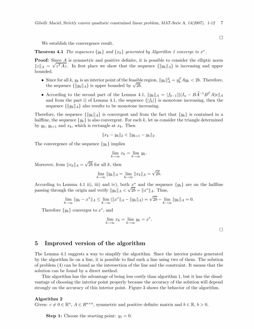
5 Improved version of the algorithm

The Lemma 4.1 suggests a way to simplify the algorithm. Since the interior points generatedby the algorithm lie on a line, it is possible to find such a line using two of them. The solutionof problem (4) can be found as the intersection of the line and the constraint. It means that thesolution can be found by a direct method.

This algorithm has the advantage of being less costly than algorithm 1, but it has the disad-vantage of choosing the interior point properly because the accuracy of the solution will dependstrongly on the accuracy of this interior point. Figure 3 shows the behavior of the algorithm.

Algorithm 2Given: c 6= 0 ∈ Rn, A ∈ Rn×n, symmetric and positive definite matrix and b ∈ R, b > 0.

Step 1: Choose the starting point: y1 = 0.


........

.............................................

.......................

...........................

...................................

..................................................

....................................................................................................................................................................................................................................................................................................................................................................................................................................................................................................................................................................................................................................................................................................................................................................................................................................

.............................................................

.......................................

...................................................................................................................• y1

........................................................................................................................................................................

x(t) = y1 − tc

• y2

....................................

...................................

...................................

...................................

...................................

...................................

...................................

...................................

...................................

...................

x(t) = y1 + t(y2 − y1)

•x1

•x∗

xTAx = 2b

Figure 3: The behavior of the direct method

Step 2: Find a border point x1 as the intersection between the halfline passing throughy1 in the direction v = −c and the constraint.

Step 3: Find an interior point y2 as the center of the resulting intersection between thelevel hyperplane cTx = cTx1 and the constraint.

Step 4: Find the solution x∗ as the intersection between the halfline passing through y1

in the direction v = y2 − y1 and the constraint.Let us analyze each step of the algorithm. There are no comments about Step 1, Step 2

and Step 3 because they are similar to those of Algorithm 1.Let us consider Step 4. Since y1 = 0, the point x∗ is obtained as the intersection between

the halfline x(t) = ty2, t > 0, and the quadratic constraint xTAx = 2b. Then,

(ty2)TA(ty2) = 2b, t∗ =

√2b

yT2 Ay2

, x∗ = t∗y2.

Then, Algorithm 2 is established as

Algorithm 2:

Given: c 6= 0 ∈ Rn, A ∈ Rn×n symmetric and positive definiteb ∈ R, b > 0.Compute: B, e and A = BT AB.

Step 1: Choose a starting interior point: y1 = 0.

Step 2: Find a border point: x1 = −

√2b

cTAcc.

Step 3: Find an interior point: y2 = By2 + f1e with y2 = argmin12xT Ax − dT x,

where f1 = cTx1 and d = −f1BT Ae.

Step 4: Find the solution: x∗ =

√2b

yT2 Ay2

y2.

6 Numerical experience

In this section implementations of Algorithms 1 and 2 are described. The algorithms have beenimplemented in Matlab in an environment PC with a Pentium 4 processor with 512 MB RAM


and 2.40GHz.The specific procedure used is given below.

• The stopping criterion used in Algorithm 1 is: ek = ‖yk − xk‖ < 10−12.

• In Step 1 of Algorithm 1 and Step 3 of Algorithm 2 the point yk = argmin 12 xT Ax− dk

Tx

is obtained by applying the spectral gradient method. It is a relatively novel non-descentmethod, appropriate to large scale optimization problems and competitive with the tradi-tional conjugate gradient method. For more details see [5, 7, 8, 9].

In the tables, the following abbreviations are used:

• n: the number of variable of the problem.

• it: the amount of iterations carried out by Algorithm 1.

• Nit: the number of iteration considered from Algorithm 1.

• it SG: the number of iterations required by spectral gradient method to obtain yk =

argmin12xT Ax − dk

Tx in the k-th iteration.

• fk = cTxk: the objective function value at the k-th iteration.

• ek =‖yk − xk‖

‖xk‖: the relative error in the k-th iteration.

• f∗ = cTx∗: the objective value function at the estimate x∗, given by the algorithm.

• r = ‖12x∗T

Ax∗ − b‖: the error constraint evaluated at x∗. We observe that r should bezero since the solution must satisfy the constraint.

• CPU time: the computing time required by the algorithm.

Now, we consider two problems, each of them with different number of variables. Bothproblems are considered without the linear term (d = 0) because any other problem can bereduced to this case.

Problem 1:Let us consider problem (4) with c = (1, 1, ..., 1)T ∈ Rn, A = diagonal(1, 2, ..., n) ∈ Rn×n

and b = 1.Table 1 shows the results obtained at each iteration of the iterative method with n = 100.

Tables 2 and 3 show the results obtained applying Algorithms 1 and 2 with different values ofn (n =100, 200, 300, 400, 500, 600, 700, 800, 900 and 1000).

The fast convergence of the algorithm can be observed in Table 1: the error decreases quitefast. Also, it is possible to observe that the number of iterations required by the spectral gradientmethod to obtain yk decreases as k increases.

Table 2 shows that the number of iterations required by Algorithm 1 do not increase whenthe number of variable is augmented. The time required to run the algorithm increases becauseof the operations needed at each iterations. Clearly, more computing time is needed if thenumber of variable is large.

Comparing Tables 2 and 3, there are not significant differences between the results obtainedby Algorithms 1 and 2, despite the considerable decrease in computing time.


Nit fk = cTxk ek = ‖yk−xk‖‖xk‖

it SG

1 −1.99007438041998 1 02 −2.96984668055811 0.18218129703840 1323 −3.20683507409673 0.03193981609218 1234 −3.22093665958930 0.00178265648084 1115 −3.22098665492903 6.297052951447885e− 006 946 −3.22098665555746 7.915125095980291e− 011 767 −3.22098665555746 5.035955884656709e− 017 18

Table 1: Iterations of Algorithm 1 - Problem 1, n = 100

n f∗ = cT x∗ r = ‖12x∗TAx∗ − b‖ CPU time It

100 −3.22098665555746 3.330669073875470e− 016 0.0630 7200 −3.42871140463044 2.220446049250313e− 016 0.3430 7300 −3.54476060695204 3.330669073875470e− 016 1.4530 7400 −3.62489439602770 2.220446049250313e− 015 2.9850 7500 −3.68587124842703 9.992007221626409e− 016 5.9680 7600 −3.73496410209512 2.220446049250313e− 015 11.1250 7700 −3.77597937377608 1.332267629550188e− 015 18.9220 7800 −3.81115527428657 9.992007221626409e− 016 27.3750 7900 −3.84191771929092 1.110223024625157e− 015 38.9690 71000 −3.86923011994643 2.220446049250313e− 016 56.9370 7

Table 2: Algorithm 1 applied to Problem 1 and different values of n

n f∗ = cT x∗ r = ‖12x∗TAx∗ − b‖ CPU time

100 −3.22098665555746 2.220446049250313e− 016 0.0320200 −3.42871140463045 8.881784197001252e− 016 0.1250300 −3.54476060695204 1.887379141862766e− 015 0.6400400 −3.62489439602770 8.881784197001252e− 016 1.4530500 −3.68587124842704 8.881784197001252e− 016 2.9850600 −3.73496410209512 1.332267629550188e− 015 5.3910700 −3.77597937377609 8.881784197001252e− 016 9.0470800 −3.81115527428656 5.551115123125783e− 016 12.5630900 −3.84191771929092 1.110223024625157e− 016 18.79701000 −3.86923011994643 9.992007221626409e− 016 24.8750


Problem 2:

Let us consider problem (4) with c = (1, 1, ..., 1)T ∈ Rn, b = 1 and A =H(v)TH(v)

n3∈ Rn×n,

where v = (1, 2, 3, ..., n) ∈ Rn and H(v) is a square Hankel matrix whose first column is v andwhose elements are zero below the first anti-diagonal. This matrix is symmetric and positivedefinite.

Table 4 shows the results obtained at each iteration of the algorithm when n = 100. Tables


5 and 6 show the results obtained via Algorithms 1 and 2.

Nit fk = cTxk ek = ‖yk−xk‖‖xk‖ it SG

1 −3.82499150774954 1 02 −7.25025696447532 0.09187993351090 8753 −10.07701880238112 0.04035743849082 7054 −12.17872638695642 0.02164347403184 7535 −13.51681325907164 0.01141576228632 8786 −14.16487459323087 0.00498514448544 6957 −14.34312557007998 0.00130895964353 7328 −14.35752222964941 1.044190646555198e− 004 7109 −14.35761670656568 6.845619643013136e− 007 58010 −14.35761671063453 2.948193549052210e− 011 33211 −14.35761671063453 0 27

Table 4: Iterations of Algorithm 1 - Problem 2, n = 100

n f∗ = cT x∗ r = ‖12x∗TAx∗ − b‖ CPU time It

100 −14.35761671063453 0 0.4060 11200 −20.15598398495877 0 5.8910 13300 −24.62326461541155 1.110223024625157e− 016 25.4060 15400 −28.39588023323513 0 78.4690 17500 −31.72283979772807 2.220446049250313e− 016 198.0780 18


n f∗ = cTx∗ r = ‖12x∗TAx∗ − b‖ CPU time

100 −14.35761671063453 2.220446049250313e− 016 0.0630200 −20.15598398495877 0 0.7500300 −24.62326461541155 2.220446049250313e− 016 2.1880400 −28.39588023323513 0 7.4060500 −31.72283979772806 2.220446049250313e− 016 13.3750


The observations done above are valid for Problem 2. However, it is possible to observe anincrement in the number of iterations required by Algorithm 1 to achieve convergence. Moreover,it is possible to observe that the computing time required for running Problem 2 is higher thanthe one required for Problem 1. It is because in Problem 1, the matrix is sparse.

7 Conclusions

The problem of minimizing a linear function subject to a strictly convex quadratic constrainthas been analyzed. The convergence of the algorithm is guaranteed via simple geometric consid-erations. The simplicity and the good behavior of proposed algorithm make it adequate to large


scale optimization problems. Since many topologic optimization problems are established as(1) the next objective is to extend the algorithm when the strictly convex quadratic constraintsappear showing a block structure. The truss optimization problems, if many bars are involved,show this block structure and the extended algorithm might be successfully used.

References

[1] A. BEN-TAL and M.P. BENDSØE. A new method for optimal truss topological design.SIAM Journal on Optimization, 3(2):322–358, 1993.

[2] A. BEN-TAL and M. ZIBULESVSKY. Penalty/barrier multiplier methods for convexprogramming problems. SIAM Journal on Optimization, 7(2):347–366, 1997.

[3] M.P. BENDSØE and O. SIGMUND. Topology Optimization. Theory, Methods and Appli-cations. Springer Verlag, Berlin, 2003.

[4] M.P. BENDSØE, A. BEN TAL, and J. ZOWE. Optimization methods for truss geometryand topology design. Structural Optimization, 7:141–159, 1994.

[5] R. FLETCHER. On the Barzilai-Borwein method. Technical Report NA/207, Departmentof Mathematics, University of Dundee, Dundee, Scotland, 2001.

[6] F. JARRE, M. KOCVARA, and J. ZOWE. Optimal truss design by interior-point methods.SIAM Journal on Optimization, 8(4):1084–1107, 1998.

[7] M. RAYDAN. Convergence properties of the Barzilai and Borwein gradient method. PhDthesis, Dept. of Mathematical Science, Rice University, Houston, Texas, 1991.

[8] M. RAYDAN. On the Barzilai and Borwein choice of the steplength for the gradient method.IMA Journal Numerical Analysis, 13:321–326, 1993.

[9] M. RAYDAN. The Barzilai and Borwein gradient method for the large scale unconstrainedminimization problem. SIAM Journal on Optimization, 7:26–33, 1997.

[10] J. ZOWE, M. KOCVARA, and M.P. BENDSØE. Free material optimization via mathe-matical programming. Computers & Structures, 79:445–466, 1997.

MAT-Serie A, 14 (2007), 13-23 13

Thickness optimization of an elastic beam

Marıa C. Maciel ∗

Depto. de Matematica, Universidad Nacional del Sur,Av. Alem 1253, 8000 Bahıa Blanca, Argentina

Elvio A. Pilotta †

FaMAF, Universidad Nacional de Cordoba, CIEM–CONICETMedina Allende s/n, 5000 Cordoba, Argentina

Graciela N. Sottosanto ‡

Depto. de Matematica, Universidad Nacional del Comahue,

Santa Fe 1400, 8300 Neuquen, Argentina

Abstract

An elastic beam of variable thickness subject to a vertical load is considered in thiswork. Finding the thickness distribution minimizing the compliance of the beam is thestructural optimization problem to be solved. Different types of support conditions forthe beam are also included in the analysis. The approach is based on the Haslingerand Makinen formulation, although the resulting optimization problem is solved in adifferent way. Finite elements method is used to obtain a suitable discretized problem.The optimization problem is solved by using interior point methods and trust-regionstrategies. Numerical results are reported.

Resumen

En este trabajo es considerada una viga de espesor variable sujeta a una carga ver-tical. El problema de optimizacion estructural a resolver consiste en hallar el espesorque minimiza la deformacion de la viga. Se analiza el problema con diferentes tipos decondiciones de soporte en la viga. El trabajo esta basado en la formulacion propuestapor Haslinger y Makinen aunque el problema de optimizacion obtenido es resuelto con unmetodo diferente. El metodo de elementos finitos es utilizado para formular el problemadiscreto. El problema de optimizacion es resuelto usando el metodo de puntos interioresy estrategias de region de confianza. Se muestran resultados numericos.

Key words: nonlinear programming, structural optimization, finite element method.Palabras Claves: programacion no lineal, optimizacion estructural, metodo de elementos

finitos.AMS Subject Classification: 74P05, 65L60, 90C30, 90C51.

∗[email protected]†[email protected]‡[email protected]

This work was supported by Fundacion Antorchas, Grant 13900/4, the Universidad Nacional del Sur, GrantUNS 24/L069, the Universidad Nacional del Comahue, Grant E060 and SECYT-UNC.

Maciel-Pilotta-Sottosanto, Thickness optimization of an elastic beam 14

1 Introduction

Our main objective in this work is to present an optimization model for solving a structuraldesign problem. Particularly, we are interested in sizing optimization problems, where a typicalsize of a structure has to be optimized.

The model problem that we considered is well known in the structural optimization liter-ature, however, the modelization technique presented here is simple because it avoids usingcomplex tools and aspects from the sensitivity analysis. The sensitivity analysis is the usualtheory for dealing this kind of problem (see [7, 12]). However, the computational aspects andnumerical implementation based on it use to be sophisticated (see [1, 5, 8]).

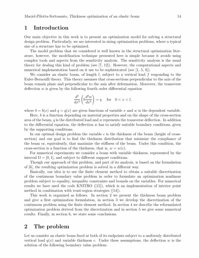
We consider an elastic beam, of length l, subject to a vertical load f responding to theEuler-Bernoulli theory. This theory assumes that cross-sections perpendicular to the axis of thebeam remain plane and perpendicular to the axis after deformation. Moreover, the transversedeflection w is given by the following fourth order differential equation

d2

dx2

(

bd2w

dx2

)

= q for 0 < x < l,

where b = b(x) and q = q(x) are given functions of variable x and w is the dependent variable.Here, b is a function depending on material properties and on the shape of the cross-section

area of the beam, q is the distributed load and w represents the transverse deflection. In additionto the differential equation, the deflection w has to satisfy suitable boundary conditions, givenby the supporting conditions.

In our optimal design problem the variable e is the thickness of the beam (height of cross-section) and our goal is to find the thickness distribution that minimize the compliance ofthe beam or, equivalently, that maximize the stiffness of the beam. Under this condition, thecross-section is a function of the thickness, that is, w = w(e).

For numerical experiments we consider a beam with variable thickness, represented by theinterval Ω = [0, 1], and subject to different support conditions.

Though our approach of this problem, and part of its analysis, is based on the formulationof [6], the resulting optimization problem is solved in a different way.

Basically, our idea is to use the finite element method to obtain a suitable discretizationof the continuous boundary value problem in order to formulate an optimization nonlinearproblem subject to equality, inequality constraints and bounds on the variables. For numericalresults we have used the code KNITRO ([15]), which is an implementation of interior pointmethod in combination with trust-region strategies ([14]).

This work is organized as follows. In section 2 we present the thickness beam problemand give a first optimization formulation, in section 3 we develop the discretization of thecontinuous problem using the finite element method. In section 4 we describe the reformulatedoptimization problem derived from the discretization and in section 5 we give some numericalresults. Finally, in section 6, we state some conclusions.

2 The problem

Let us consider an elastic beam fixed at both of its endpoints subject to a uniformly distributedvertical load q(x) and variable thickness e. Under these assumptions, the deflection w is thesolution of the following boundary value problem:


d2

dx2

(

βe(x)3 d2w

dx2

)

= q(x), 0 < x < l, (2.1)

w(0) = w(l) =dw

dx(0) =

dw

dx(l) = 0,

where β ∈ L∞([0, l]) is a positive function depending on material properties and on the shapeof the cross-section area of the beam.

The stiffness of the beam is characterized by the functional J : H20 (Ω) →

defined as

J(w(e)) =∫ l

0q(x)w(e)dx,

where H20 (Ω) represent the Sobolev space of functions whose second derivatives are square-

integrable and satisfy the boundary conditions and w(e) is the solution of the boundary valueproblem (2.1).

This functional, which represents the external energy of deformation, can be considered asa measure of flexibility of the beam. On the other hand, the decrease of this functional impliesincreasing of the stiffness, so the problem of maximizing the stiffness is equivalent to minimizethe functional J . This functional frequently appears in structural optimization either in theobjective function or in the constraint set of the problem ([2, 13]).

To formulate the mathematical problem, we add some conditions, besides (2.1), that thethickness e has to satisfy. This conditions define a set of admissible thicknesses C given by:

C =

e ∈ C0,1(Ω) | 0 < emin ≤ e ≤ emax in Ω,|e(x1) − e(x2)| ≤ γ|x1 − x2| for all x1, x2 ∈ Ω,∫ l0 e(x)dx = α, for some α > 0,

e is symmetrical in Ω

,

i.e., C consists of functions that are uniformly bounded, uniformly Lipschitz continuous in [0, l]and preserve the beam volume and due to the boundary conditions a symmetric property isrequired. All of such conditions make sense from the practical and physical point of view.

From numerical and implementation aspects we consider the set C characterized by contin-uous and piecewise constant thickness functions. This last requirement implies to construct astepped beam. Consequently, the optimization problem is given by

Find e? ∈ C such that

w(e?) = argmin J(w(e)) = argmin∫ l

0q(x)w(e(x))dx

where w(e) satisfy the problem (2.1).

To solve numerically this problem, we make a complete discretization of it, and we obtaina new problem defined by a finite number of design parameters.

3 Discretization of the State Problem

For a discretization of the continuous problem we use a finite element approach, that is, wediscretize the domain Ω and write the weak formulation of the differential equation. See [11, 10].


Let d ∈ be given and ∆h : 0 = a0 < a1 < . . . < ad = l be an equidistant partition of Ωwith the step h = l/d, ai = ih, i = 0, . . . , d. Thus, we divide the interval Ω in d subintervalscalled elements. The ai, i = 0 . . . , d are called nodes.

In order to obtain the weak formulation we consider an arbitrary element Ωk = [ak, ak+1].Let Vh be a finite dimensional subspace of H2

0 (Ω), whose functions are continuous piecewisepolynomials. Let v ∈ Vh be an arbitrary test function.

Now, by using the standard integration-by-parts formula twice in Ωk, we have

∫ ak+1

ak

(

βe3 d2v

dx2

d2w

dx2− vq

)

dx +

[

vd

dx

(

βe3d2w

dx2

)

−dv

dxβe3 dw

dx2

]ak+1

ak

= 0.

The variables at each node involve the deflection w and its derivative dwdx

.In the case of a beam supporting a flexion, the terms which have to be evaluated at the

endpoints, have structural interpretations ([10]). Thus, the natural boundary conditions in-

volve specifications about the bending moment βe3 d2wdx2 and the shear force d

dx

(

βe3 d2wdx2

)

at theendpoints.

For simplicity, we introduce the following notation

Qk1 =

[

ddx

(

βe3 d2wdx2

)]

ak

, Qk2 =

[

βe3 d2wdx2

]

ak

,

Qk3 = −

[

ddx

(

βe3 d2wdx2

)]

ak+1

, Qk4 = −

[

βe3 d2wdx2

]

ak+1

.

Thus, the weak formulation is given by

0 =∫ ak+1

ak

(

βe3 d2v

dx2

d2w

dx2− vq

)

dx − v(ak)Qk1 (3.1)

−

(

−dv

dx

)

Qk2 − v(ak+1)Q

k3 −

(

−dv

dx

)

Qk4.

See Fig. 1.The variational formulation (3.1) requires that the interpolation functions to be twice contin-

uously differentiable and has to satisfy interpolation conditions at the endpoints: w(ak), w(ak+1), w′(ak), w′(ak+1).These four conditions imply that we need a cubic polynomial to interpolate w(x) and we assignthe nodal variables for the element Ωk

u1 = w(ak), u2 = −w′(ak)u3 = w(ak+1), u4 = −w′(ak+1).

By using these nodal variables we have the following expression for w in Ωk

w(x) = u1φ1(x) + u2φ2(x) + u3φ3(x) + u4φ4(x) (3.2)

=4∑

j=1

ujφj(x),

where the functions φj are the cubic Hermitte polynomials.


Figure 1: Generalized forces at one element of the beam.

3.1 The Finite Element Model

According to (3.2) and the interpolation functions φj in the weak formulation (3.1) we obtainthe finite element model for the Euler-Bernoulli beam. Since there are four nodal variables ateach element, then four possible choices could be used for v: v = φi, i = 1, . . . , 4.

For simplicity we consider the function β with constant value at the whole beam. Therefore,for the i-th algebraic equation (for v = φi) we have that

0 = βe3k

4∑

j=1

(

∫ ak+1

ak

d2φkj

dx2

d2φki

dx2dx

)

uj

−∫ ak+1

ak

φki q(x)dx − Qk

i ,

or equivalently,4∑

j=1

Kkiju

kj − F k

i = 0,

where

Kkij = βe3

k

∫ ak+1

ak

d2φkj

dx2

d2φki

dx2dx,

F ki =

∫ ak+1

ak

φki q(x)dx + Qk

i .

Now, if we write these coefficients in matrix notation we have

Kk11 Kk

12 Kk13 Kk

14

Kk21 Kk

22 Kk23 Kk

24

Kk31 Kk

32 Kk33 Kk

34

Kk41 Kk

42 Kk43 Kk

44

uk1

uk2

uk3

uk4

=

qk1

qk2

qk3

qk4

+

Qk1

Qk2

Qk3

Qk4

,

where the matrix of the system, which is symmetric, is the stiffness matrix for the k-th elementof the beam and the right hand side term is the vector of generalized forces, including theapplied external forces and the shear force and flexion at the endpoints of the element.


If h is the length of the element and e is the thickness, the above equation is given by

Kk =2βe3

k

h3

6 −3h −6 −3h−3h 2h2 3h h2

−6 3h 6 3h−3h h2 3h 2h2

,

F k =qh

12

6−h

6h

+

Q1

Q2

Q3

Q4

.

See [11].

3.2 Element Assembly

Having calculated the matrices and equations describing our approximations over each finiteelement, the next step is to assemble these equations on the entire mesh adding up the contri-butions furnished by each element. To do this, we take into account the two degrees of freedomat each node. That is, we consider the relationship between the variables associated to the rightnode at one particular element and the left node to the next element. In particular we con-sider the equilibrium relationships between the bending moment and the shear force betweenelements.

When the beam is partioned in d elements we obtain a 2(d+1)× 2(d+1) assembly matrix.However, the algebraic system has 4(d + 1) unknown variables, 2(d + 1) correspond to thegeneralized forces vector and the other 2(d+1) to the deformations and its derivatives. Imposingthe boundary conditions and the applied loads will allow us to reduce the unknown variables.

The boundary conditions for the beam problem depend on the geometric nature of thesupport conditions.

In the particular case of a beam fixed at both endpoints the deflection w and its derivativedwdx

are zero at the endpoints. The equilibrium conditions, at the intermediate nodes, yield theequations

Qk3 + Qk+1

1 = 0, Qk4 + Qk+1

2 = 0,

because there are no forces applied there, whereas the shear force and the bending moment areunknown at the endpoints of the beam.

Now, by using the equilibrium conditions at the intermediate nodes we have the nonlinearsystem

K(e)U(e) = F (e),

where K(e) is the stiffness matrix

6e31 −3he3

1 . . . 0 0 0−3he3

1 2h2e31 . . . 0 0 0

−6e31 3he3

1 6(e31 + e3

2) . . . 0 0−3he3

1 h2e31 3h(e3

1 − e32) . . . 0 0

......

......

......

0 . . . . . . 3h(e3d−1 − e3

d) −6e3d −3he3

d

0 . . . . . . 2h2(e3d + e3

d−1) 3he3d h2e3

d

0 . . . . . . 3he3d 6e3

d 3he3d

0 . . . . . . h2e3d 3he3

d 2h2e3d


and

U(e) =

00u3......

u2d

00

, F (e) =qh4

24β

6−h

12......6h

+

Q11

Q12

0...0

Qd3

Qd4

.

Since the equations that contain deflections and its slopes do not contain the unknowncoefficients associated to the generalized forces, the corresponding equations can be solvedindependently. Thus, the matrix equation can be partitioned

K11 K12 K13

K21 K22 K23

K31 K32 K33

U1

U2

U3

=

F 1

F 2

F 3

,

where U1 and U3 contain the known deflection and derivatives (in this case are zero due thesupport conditions) and U 2 are the unknown. At the right hand side, in F 1 and F 3 there areunknown coefficients. Under this conditions the matrix equation that we are interested in, canbe expressed as

K22U2 = F 2. (3.3)

This is a 2(d−1)×2(d−1) system, whose unknown variables are the deflection and derivativesat the intermediate nodes of the discretization. The coefficients of the submatrix K22 dependon the thickness of each element of the beam.

4 Reformulation of the Optimization Problem

The discretization of the state problem yields a system of nonlinear algebraic equations (3.3).For the sake of simplicity of notation we rewrite the system (3.3) as

K(e)U(e) = F, (4.1)

where U(e) contains the deflection and its derivatives at the intermediate nodes. For thenumerical solution of the problem we have to consider the conditions for the admissible thicknessand discretization of the objective function.

The discretization of the state problem concern to the functional J , however, the restrictionof J to the subspace Vh is identified with another functional defined in the euclidean space 2(d−1) as in [6].

To do this, we discretize the integral by using the same numerical formula that we have usedfor the volume of the beam. Since we consider uniformly distributed load, that is q(x) = q,constant at the whole beam, and we also assume that the thickness is constant at each elementit is enough to use the rectangle rule. Clearly, if the load were not uniformly distributed it wouldbe better to use a higher order quadrature rule. Then, the objective function is approximatedby

J(u(e)) =∫ l

0q(x)u(e(x))dx ' qT U ,


where U contains only the d−1 components of U(e) associated to deflections at the intermediatenodes and q is a constant vector, which has the same size.

Since the discretized beam is stepped constant, the admissible thickness is defined by apiecewise constant function that satisfies the following conditions

emin ≤ ei ≤ emax, i = 1, . . . , d,

| ei+1 − ei |≤ γh, i = 1, . . . , d − 1,

for some constant γ. Moreover, the preserving volume condition is given by

hi=d∑

i=1

ei = α.

Finally, the optimization problem is given by

mine,U

qT U

s.t. K(e)U(e) = F

hi=d∑

i=1

ei = α,

emin ≤ ei ≤ emax, i = 1, . . . , d,

| ei+1 − ei |≤ γh, i = 1, . . . , d − 1.

Thus, the above problem is the classical formulation of a nonlinear programming problem withbounds at the variables and equality and linear inequality constraints. It is worth noting thatsystem of algebraic equations (4.1) is nonlinear strongly on the design variables ei. Throughthe derivation of the model is similar to the presentation in [6], the formulation is conceptuallydifferent. In our approach the variables corresponding to thickness and deflection are relatedthrough the constraint equation KU = F , although initially they are independent. Moreover,in that presentation the optimization problem take into account the thicknesses and their rela-tionship with the deflections trough a sensitivity analysis. While sensitivity analysis provides anelegant and mathematically rigorous method to formulate the problem, it has one very seriousdrawback: the numerical solution is very difficult to be computed.

5 Numerical Experiments

For numerical experiments we consider a beam with two different support conditions. First,we analyze a beam with both endpoints fixed, whose discretized model has been described inprevious sections. Then, we consider a beam with one endpoint fixed and the other one simplysupported. For this case, we note that the boundary conditions are different. At the simplysupported endpoint the deflection is zero whereas its derivative is not: this support conditiondoes not allow to assimilate bending moment at this endpoint. By using the notation of section3, we have

w(0) = u11 = 0;

dw

dx

x=0= u1

2 = 0;


w(l) = ud3 = 0; Qd

4 = −

[

βe3d

d2w

dx2

]

l

= 0.

According to these boundary conditions the nonlinear system of algebraic equations from thefinite element method is modified.

For solving the optimization problem, we have used the solver KNITRO 3.1 ([14, 15]), bymeans of a Visual Fortran interface. The user has to provide three subroutines including thedata of the problem, the objective function and the constraints, and finally, the gradient of theobjective function and the Jacobian matrix of the constraints. This code is an implementationof the interior point method, where the nonlinear programming problem is solved by means ofthe solution of a sequence of barrier subproblems, depending on a parameter µ. On the otherhand, the algorithm uses a trust-region method as a globalization strategy and a merit functionto obtain global convergence results.

Each iteration of the subalgorithm generates steps whose normal and tangential componentssatisfy mild conditions on adequate models. The normal component improves the feasibilityand the tangential component, which is computed using the projected conjugated gradientmethod, improves the optimality. The whole code KNITRO 3.1 computes some iterations foreach subproblem before the barrier parameter is decreased and then the procedure is repeateduntil suitable convergence conditions are reached. See [4, 3] for a complete description andanalysis of this method.

The number of elements used for numerical experiments in both problems was d = 8 andd = 32. For simplicity we adopted the following default values:

- l = 1, the length of the beam.

- β = 1; q(x) = −1, the uniformly distributed load.

- emin = 0.01, emax = 0.1, bounds for the thickness.

- α = 0.05, γ = 0.5.

The initial approximation for thickness were ei = 0.05, i = 1, . . . , d. Then we solved thelinear system of algebraic equations (4.1) in order to obtain the initial values for the othervariables.

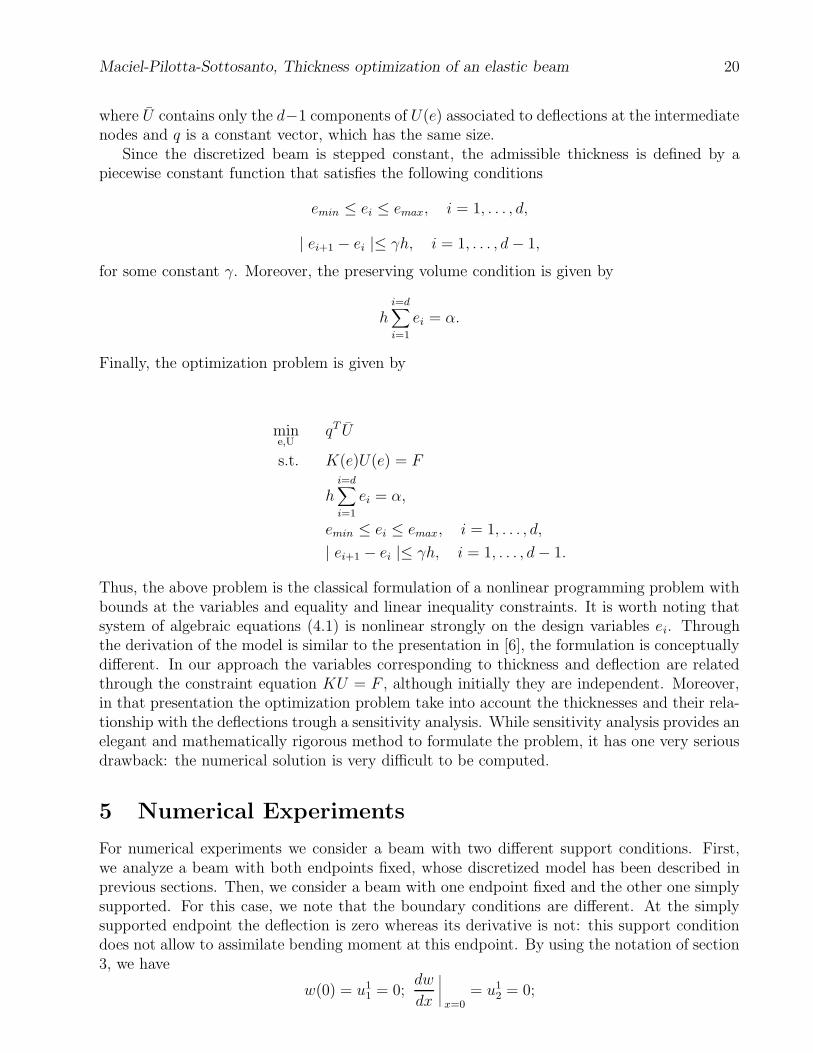
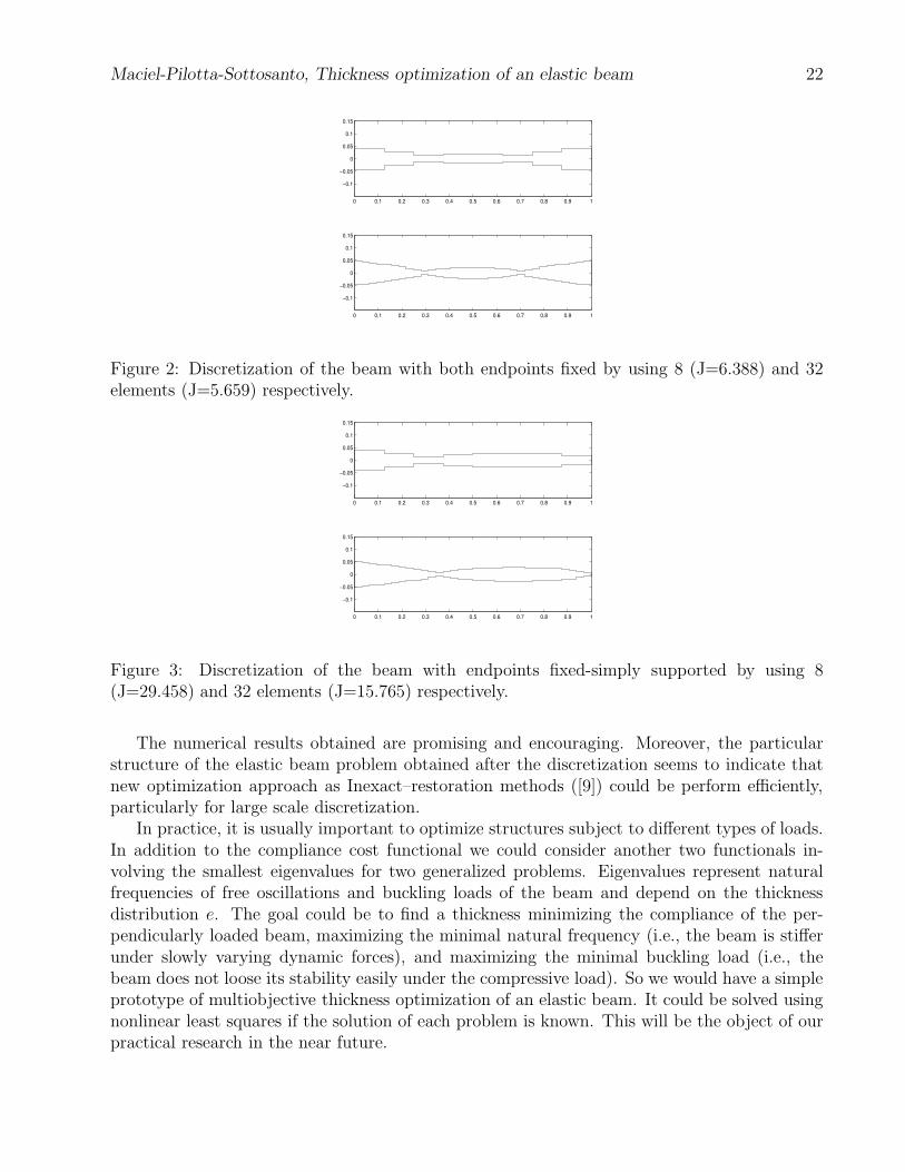
Finally, we show in Fig. (2–3), the profile of the optimal solution for the beam problem, inboth cases, and the corresponding optimal value of the objective function.

6 Conclusions

We have presented and tested an optimization formulation for the elastic beam problem, whichis subject to vertical loads, as in Euler-Bernoulli theory.

One of the main advantage of this formulation is that it is possible to use any of the manyavailable nonlinear programming method to solve the thickness problem. It is a very attractivefeature due to the advances in optimization algorithm during the last years. On the otherhand, researchers in engineering, applied mathematics and other sciences paid attention to theconexion between optimization and computational mechanics in structural problems (structuraloptimization), so important and interesting advances were done about this area recently.

Though we considered here a one dimensional model, the same ideas can be applied in morecomplicated structural problems of dimension 2 or 3, or subject to different support and loads.


0 0.1 0.2 0.3 0.4 0.5 0.6 0.7 0.8 0.9 1

−0.1

−0.05

0

0.05

0.1

0.15

0 0.1 0.2 0.3 0.4 0.5 0.6 0.7 0.8 0.9 1

−0.1

−0.05

0

0.05

0.1

0.15

Figure 2: Discretization of the beam with both endpoints fixed by using 8 (J=6.388) and 32elements (J=5.659) respectively.

0 0.1 0.2 0.3 0.4 0.5 0.6 0.7 0.8 0.9 1

−0.1

−0.05

0

0.05

0.1

0.15

0 0.1 0.2 0.3 0.4 0.5 0.6 0.7 0.8 0.9 1

−0.1

−0.05

0

0.05

0.1

0.15

Figure 3: Discretization of the beam with endpoints fixed-simply supported by using 8(J=29.458) and 32 elements (J=15.765) respectively.

The numerical results obtained are promising and encouraging. Moreover, the particularstructure of the elastic beam problem obtained after the discretization seems to indicate thatnew optimization approach as Inexact–restoration methods ([9]) could be perform efficiently,particularly for large scale discretization.

In practice, it is usually important to optimize structures subject to different types of loads.In addition to the compliance cost functional we could consider another two functionals in-volving the smallest eigenvalues for two generalized problems. Eigenvalues represent naturalfrequencies of free oscillations and buckling loads of the beam and depend on the thicknessdistribution e. The goal could be to find a thickness minimizing the compliance of the per-pendicularly loaded beam, maximizing the minimal natural frequency (i.e., the beam is stifferunder slowly varying dynamic forces), and maximizing the minimal buckling load (i.e., thebeam does not loose its stability easily under the compressive load). So we would have a simpleprototype of multiobjective thickness optimization of an elastic beam. It could be solved usingnonlinear least squares if the solution of each problem is known. This will be the object of ourpractical research in the near future.


References

[1] ARORA J. S., Introduction to optimal design. McGraw-Hill Book Company, New York(1989).

[2] BENDSØE M. P., Topology optimization. Theory, methods and applications, SpringerVerlag, Berlin, (2002).

[3] BYRD R. H., GILBERT C. & NOCEDAL J., A trust region method based on interiorpoint techniques for nonlinear programming, Mathematical Programming 89(1), (2000),pp. 149–185.

[4] BYRD R. H., HRIBAR M.E. & NOCEDAL J., An interior point algorithm for large scalenonlinear programming, SIAM Journal on Optimization, 9(4), (1999), pp. 877–900.

[5] HAFTKA R.T., GURDAL Z. & KAMAT M.P., Elements of structural optimization, 2nd.rev. ed., Kluwer Academic Publishers, Dordrecht, The Netherlands, (1990).

[6] HASLINGER J. & MAKINEN R.A., Introduction to Shape Optimization. Theory, Ap-proximation, and Computation. SIAM, Philadelphia (2003).

[7] HAUG E.J., CHOI K. K. & KOMKOV V., Design sensitivity analysis of structural systems,Academic Press, Orlando, FL, USA (1986).

[8] HAUG E.J. & ARORA S., Applied Optimal Design, John Wiley & Sons, New York (1979).

[9] MARTINEZ J. M. & PILOTTA E. A., Inexact–Restoration algorithm for constrainedoptimization, Journal of Optimization Theory and Applications 104(1), (2000), pp. 135–163.

[10] REDDY J. N., An Introduction to the finite element method, McGraw–Hill, Inc., USA(1993).

[11] SCHWARZ, H.R., Finite element methods, Academic Press, San Diego, CA, USA (1988).

[12] SOKOLOWSKI J. & ZOLESIO J. P., Introduction to shape optimization: shape sensitivityanalysis, Springer-Verlag, Berlin (1992).

[13] SVANBERG K., On the convexity and concavity of compliances, Structural OptimizationVol 7, (1994), pp. 42–46.

[14] WALTZ R.A., MORALES J.L., NOCEDAL J. & ORBAN D., An interior algorithm fornonlinear optimization that combines line search and trust–region steps, Tech. Rep. OTC2003-6, Northwestern University, Evanston, IL (2003).

[15] WALTZ R.A. & NOCEDAL J., Knitro User’s Manual, Version 3.1. Tech. Rep. OTC 2003-5,Optimization Technology Center, Northwestern University, Evanston, IL (2003).

Determinación de dos coeficientes térmicos a travésde un problema de desublimación con acoplamiento

de temperatura y humedad. ∗

María Fernanda NATALE (1) - Eduardo A. SANTILLAN MARCUS (1)

Domingo A. TARZIA (1)(2)

(1)Depto. de Matemática, F.C.E.,Universidad Austral,Paraguay 1950, S2000FZF Rosario, ARGENTINA

(2) CONICET, ARGENTINAE-mail: [email protected];

[email protected]; [email protected]

Resumen

Se considera un modelo de flujo de calor y humedad a través de un semiespacio poroso du-rante congelamiento, con sobrecondición de temperatura y de flujo de calor en el borde fijopara la determinación de dos coeficientes desconocidos del material semi-infinito de cam-bio de fase. Se trata de un problema de frontera móvil con acoplamiento de las funcionestemperatura y concentración (ecuaciones de tipo Luikov) con ocho parámetros. Para dosde los casos de determinación posibles, se hallan condiciones necesarias y suficientes parala existencia de una solución y las fórmulas correspondientes para las temperaturas yconcentraciones de ambas fases, como también para los coeficientes desconocidos.

Nomenclaturaam difusividad de humedadci, i = 1, 2 calor específico en la fase-iki, i = 1, 2 conductividad térmica de la fase-iq0 coeficiente que caracteriza el flujo de calor en x = 0r calor latentes(t) posición del frente de evaporaciónt tiempoTi, i = 1, 2 temperatura en la fase-i.t0 temperatura inicialts temperatura en el borde fijo x = 0

∗MAT - Serie A, 14 (2007), 25-30.

25

Natale-Santillan Marcus-Tarzia, MAT-Serie A, 14 (2007), 25-30 26

tv temperatura de cambio de fase (ts < tv < t0)u potencial de transferencia de masau0 potencial inicial de transferencia de masaρ densidad de masaδ coeficiente de gradiente térmicoσ constante que caracteriza la frontera móvil s(t) = 2σ

√t

Lu = ρamc2k2

número de LuikovKo = ruo

c2(t0−tv) número de Kossovitch

Pn = δ(t0−tv)uo

número de Posnov

1. Introducción.Los problemas de transferencia de calor y masa con cambio de fase que se llevan a cabo

en un medio poroso, tales como evaporación, condensación, congelamiento, derretimiento,sublimación y desublimación, tienen una gran aplicación en procesos de separación, tec-nología de alimentos, migración de calor en terrenos y suelos, etc. Debido a que estetipo de problemas es no lineal, el resolverlos usualmente tiene dificultades matemáticas.Sólo se han encontrado unas pocas soluciones exactas para casos ideales (ver [2],[3],[4]por ejemplo). Una extensa bibliografía sobre problemas de frontera libre y móvil para laecuación de calor-difusión está dada en [12].La formulación matemática de la transferencia de calor y masa en cuerpos de capilares

porosos fue establecida por Luikov ([5],[6]). Mikhailov [7] presentó dos modelos diferentespara resolver el problema de la evaporación de humedad líquida desde un medio poroso.Para el problema del congelamiento (desublimación) de un semiespacio poroso húmedo,Mikhailov también presentó una solución exacta [8] para una condición de temperaturaconstante en el borde fijo x = 0. En el trabajo [9] fue presentada una solución explícitapara las distribuciones de temperatura y humedad en un semiespacio poroso con unacondición de flujo de calor en el borde fijo x = 0 del tipo q0√

t.

Ahora se considerará el modelo presentado en [8]-[9] como un problema de fronteramóvil, esto es x = s(t) es conocida (dada por la expresión s(t) = 2σ

√t con σ > 0 una

constante dada) con una sobrecondición en el borde fijo. Esto nos permite considerar doscoeficientes térmicos desconocidos y calcularlos bajo ciertas restricciones sobre los datosiniciales del problema siguiendo la idea de [13] para una fase y de [11] para dos fases.Se considera el flujo de calor y humedad a través de un semiespacio poroso durante el

congelamiento. La posición del frente de cambio de fase al tiempo t está dada por x = s (t)que divide al cuerpo poroso en dos regiones. En la región congelada, 0 < x < s (t), no haymovimiento de humedad y la distribución de temperatura está descripta por la ecuacióndel calor

∂T1∂t(x, t) = a1

∂2T1∂x2

(x, t) , 0 < x < s (t) , t > 0, a1 =k1ρc1

. (1)

La región s (t) < x < +∞ es la parte húmeda del cuerpo de capilares porosos en dondefluyen acoplados el calor y la humedad. El proceso está descripto por el ya conocidosistema de Luikov [6] para el caso ε = 0 (ε es el factor de conversión de fase de líquido envapor) dado por

∂T2∂t(x, t) = a2

∂2T2∂x2

(x, t) , x > s (t) , t > 0, a2 =k2ρc2

(2)


∂u

∂t(x, t) = am

∂2u

∂x2(x, t) , x > s (t) , t > 0. (3)

Las distribuciones iniciales de temperatura y humedad son uniformes½T2 (x, 0) = T2 (+∞, t) = t0,u (x, 0) = u (+∞, t) = u0.

(4)

Se supone que sobre la superficie del semiespacio la temperatura es constante

T1 (0, t) = ts (5)

donde ts < tv.Sobre el frente de congelamiento, existe una igualdad entre las temperaturas

T1 (s (t) , t) = T2 (s (t) , t) = tv, t > 0, (6)

donde tv < t0.El balance de calor y humedad en el frente de congelamiento da lo siguiente

k1∂T1∂x

(s (t) , t)− k2∂T2∂x

(s (t) , t) = ρ r u (s (t) , t)ds

dt(t) , t > 0, (7)

∂u

∂x(s (t) , t) + δ

∂T2∂x

(s (t) , t) = 0, t > 0. (8)

Se considera además una sobre condición en el borde fijo x = 0 [1] considerando queel flujo de calor depende del tiempo de la siguiente manera

k1∂T1∂x

(0, t) =q0√t

(9)

donde q0 > 0 es un coeficiente que caracteriza el flujo de calor en el borde fijo x = 0.En este trabajo, se considerará que la frontera móvil x = s(t) definida para t > 0 con

s(0) = 0, está dada pors (t) = 2σ

√t (10)

donde σ > 0 es una constante dada (puede ser determinada por procesos experimentales).El conjunto de ecuaciones y condiciones (1)-(10) será llamado problema P.Se hallarán fórmulas para la determinación de dos coeficientes térmicos desconocidos

elegido entre ρ (densidad de masa), am (difusividad de la humedad), c1 (calor específico dela región congelada), c2 (calor específico de la región húmeda), k1 (conductividad térmicade la región congelada), k2 (conductividad térmica de la región húmeda), δ (coeficientede gradiente térmico), r (calor latente) junto con las temperaturas T1, T2 y la humedadu como función de los coeficientes térmicos y los datos t0, ts, tv, q0, u0 y σ en dos de losveintiocho casos posibles.Siguiendo [9], para el caso general Lu = ρamc2

k26= 1 se tiene que

T1 (x, t) = tv −√πq0√ρc1k1

h− erf

³γ0

x2√t

´+ erf (γ0σ)

i, 0 < x < s(t), t > 0 (11)

T2 (x, t) = tv +t0−tv

1−erf( Luam

σ)

herf³q

Luam

x2√t

´− erf(

qLuamσ)i, x > s(t), t > 0 (12)


u (x, t) = u0 − γ1 erf³q

Luam

x2√t

´−

exp ( 1Lu−1)

Luam

σ2 1−erf x2√amt√

Lu , x > s(t), t > 0

(13)con

γ0 =q

ρc1k1, γ1 =

δρamc2(t0−tv)k2−ρamc2

=Pn1Lu − 1

, (14)

donde los dos coeficientes térmicos desconocidos deben satisfacer el siguiente sistemade ecuaciones trascendentales:

γ2 exp¡− (γ0σ)2

¢− F1

³qLuamσ´= γ3σ 1 − γ1(1−

Q( σ√am

)

QLuam

σ

) (15)

erf (γ0σ) =1

γ4(16)

con

γ2 =√πq0√

c2k2ρ(t0−tv) , γ3 =q

πρc2k2

r u0(t0−tv) =

qπ LuamKo, γ4 =

√πq0√

c1k1ρ(tv−ts) (17)

donde las funciones reales F1 y Q están definidas por

F1 (x) =exp (−x2)(1− erf(x)) , Q (x) =

√πx exp

¡x2¢(1− erf(x)) (18)

con las siguientes propiedades

F1 (0) = 1, F1 (+∞) = +∞, F 01 (x) > 0 ∀x > 0 (19)

Q (0) = 0, Q (+∞) = 1, Q0 (x) > 0 ∀x > 0. (20)

De los 28 casos posibles en la presente comunicación sólo se considerará el caso de la de-terminación de los coeficientes térmicos c1, k1 y el de la determinación de los coeficientestérmicos c2, k2 .

Teorema 1: (Determinación de los coeficientes térmicos c1, k1) Si

γ5 =1γ2

⎧⎪⎨⎪⎩F1³q

Luamσ´+ γ3σ(1− γ1(1−

Q(σ√am

)

QLuam

σ

))

⎫⎪⎬⎪⎭ < 1 (21)

con γ1, γ2 y γ3 definidos en (14) y (17), y F1 y Q definidas en (18) , entonces existe unaúnica solución al problema P dada por (11)-(13), y los coeficientes térmicos k1 y c1 estándados por las siguientes expresiones

k1 =√πq0

(tv−ts)F2

⎛⎝s 1

log1γ5

⎞⎠ , c1 =√πq0

σρ(tv−ts)M

⎛⎝s 1

log1γ5

⎞⎠ (22)

donde las funciones reales F2 y M están definidas por

F2 (x) =erf (x)

x, M (x) = x erf (x) . (23)


Demostración: Considerando x =q

ρc1k1σ e y =

√ρc1k1(tv−ts)√

πq0, el sistema (15)-(16)

puede escribirse como

exp¡−x2

¢= γ5 (24)

erf (x) = y (25)

De (24) surge trivialmente que x =p− log (γ5). Notemos que x > 0 si y solamente si

0 < γ5 < 1. Teniendo en cuenta que γ5 siempre es un número positivo, considerando elLema 1 de [10] acerca del signo de m2−1

1−Q(mx)Q(x)

, así que sólo se debe imponer que γ5 debe ser

menor que uno, i.e. la condición (21). Entonces, de (25) se tiene que

y = erf³p− log (γ5)

´. Luego de algunos cálculos se obtiene (22).

Teorema 2: (Determinación de los coeficientes térmicos c2, k2) Si los datos verificanla condición

tv − tsσru0

qc1k1ρ

exp¡− (γ0σ)2

¢erf (γ0σ)

< 1 (26)

entonces existen infinitas soluciones al problema P que vienen dadas por (11-13),

c2 =k2σ2ρ

ξ2 (27)

donde ξ es una solución de la ecuación

P (x) = R (x) , x > 0 (28)

para cada k2 ∈ R+, con

P (x) = 1− amPn x2

σ2−amx2

Q(σ√am

)

Q(x), R (x) = q0

σρru0exp

£− (γ0σ)2

¤+ k2(t0−tv)√

πσ2ρru0xF1 (x) .

Demostración: Primero, los datos del problema deben verificar la condición (16).Luego, de (15) y considerando x =

qρc2k2σ se tiene que

q0σρru0

exp£− (γ0σ)2

¤+ k2(t0−tv)√

πσ2ρru0xF1 (x) = 1−

amPnx2σ2 − amx2

Q(σ√am

)

Q(x),

es decir, la ecuación (28). La función R tiene las siguientes propiedades:

R (0+) = q0σρru0

exp£− (γ0σ)2

¤, R (+∞) = −∞, R0 (x) < 0 ∀x > 0.

La función P tiene las siguientes propiedades:

P (0+) = 1, P (+∞) = 1 + Pn³1−Q( σ√

am)´> 1.

Por lo tanto, se tiene que ambas funciones se encontrarán en al menos un x > 0 si lacondición q0

σρru0exp

£− (γ0σ)2

¤> 1 se verifica. Así, teniendo en cuenta (16), se halla una

solución a la ecuación (28) si vale (26). Es sencillo ver que (27) surge de la definición dex. Este análisis puede hacerse para cualquier k2 > 0 dado.

Los veintiseis casos restantes serán considerados en un futuro trabajo que se encuentraen etapa de preparación.


Agradecimientos.Este trabajo ha sido realizado gracias al apoyo recibido del ”Fondo de Ayuda a la

Investigación” de la Universidad Austral, Rosario (Argentina).

References

[1] Cannon, J. R., The one-dimensional heat equation, Addison-Wesley, Menlo Park,1984.

[2] Cho, S. H., "An exact solution of the coupled phase change problem in a porousmedium", Int. J. Heat and Mass Transfer 18, 1139-1142 (1975).

[3] Fasano, A. - Guan, Z. - Primicerio, M. - Rubinstein, I., ”Thawing in saturated porousmedia”, Meccanica, 28, 103-109 (1993).

[4] Fasano, A. - Primicerio, M. - Tarzia, D. A., ”Similarity solutions in class of thawingprocesses”, Math. Models Methods Appl. 9, 1-10 (1999).

[5] Luikov, A. V., ”Heat and mass transfer in capillary-porous bodies”, Pergamon Press,Oxford (1966).

[6] Luikov, A. V., ”Systems of differential equations of heat and mass transfer in capillaryporous bodies”, Int. J. Heat Mass Transfer 18, 1-14 (1975).

[7] Mikhailov, M. D., ”Exact solution of temperature and moisture distributions in aporous half-space with moving evaporation front”, Int. J. Heat Mass Transfer 18,797-804 (1975).

[8] Mikhailov, M. D., ”Exact solution for freezing of humid porous half-space”, Int. J.Heat Mass Transfer 19, 651-655 (1976).

[9] Santillan Marcus, E. A. - Tarzia, D. A., "Explicit solution for freezing of humid poroushalf-space with a heat flux condition", Int. J. Eng. Science 38, 1651-1665 (2000).

[10] Santillan Marcus, E. A. - Tarzia, D. A., "Un caso de determinación de coeficientestérmicos desconocidos de un material semiinfinito poroso a través de un problemade desublimación con acoplamiento de temperatura y humedad.", MAT - Serie A 10,17-22 (2005).

[11] Stampella, M. B. - Tarzia, D. A., "Determination of one or two unknown thermalcoefficients of a semi-infinite material through a two-phase Stefan problem", Interna-tional Journal of Engineering Science 27, 1407-1419 (1989).

[12] Tarzia, D. A., "A bibliography on moving - free boundary problems for the heat-diffusion equation. The Stefan and related problems", MAT-Serie A #2 (2000) (con5869 títulos en el tema, 300 páginas). Ver www.austral.edu.ar/MAT-SerieA/2(2000).

[13] D. A. Tarzia, "Simultaneous determination of two unknown thermal coeficientsthrough an inverse one-phase Lame-Clapeyron Stefan problem with an overspecifiedcondition on the fixed face", Int. J. Heat & Mass Transfer 26 (1983) 1151 - 1157

MAT - Serie A, 14 (2007) 31-34

SOBRE LA NO CONVERGENCIA DEL METODO DE MINIMOSCUADRADOS EN DIMENSION INFINITA§

RUBEN D. SPIES(1,2,†) Y KARINA G. TEMPERINI (1,3,‡)

(1) INSTITUTO DE MATEMATICA APLICADA DEL LITORAL, IMAL, CONICET-UNL(2) DEPARTAMENTO DE MATEMATICA, FACULTAD DE INGENIERIA QUIMICA

(3) DEPARTAMENTO DE MATEMATICA, FACULTAD DE HUMANIDADES Y CIENCIAS

UNIVERSIDAD NACIONAL DEL LITORAL, SANTA FE, ARGENTINA

Resumen. Un procedimiento muy utilizado en diversas aplicaciones para aproximarlas soluciones de un problema inverso infinito-dimensional de la forma Ax = b, dondeA es un operador lineal y compacto sobre un cierto espacio de Hilbert X y b es eldato dado, consiste en encontrar una sucesion XN de subespacios aproximantes finito-dimensionales de X cuya union es densa en X y construir la sucesion xN de solucionesde mınimos cuadrados del problema en cada subespacio XN . En [3], Seidman demostroque si el problema es mal condicionado, entonces sin ninguna hipotesis adicional sobrela solucion exacta o sobre la sucesion de subespacios aproximantes XN, no se puedegarantizar que la sucesion xN convergera a la solucion exacta. En este artıculo seextiende este resultado: se prueba que si X es separable, entonces para cualquier b ∈ X,b 6= 0, y para cualquier funcion no negativa definida sobre los naturales f : IN → IR+,existe un operador lineal, compacto e inyectivo A y una sucesion creciente de subespaciosfinito-dimensionales XN ⊂ X tales que

∥∥xN −A−1b∥∥ ≥ f(N) para todo N ∈ IN, donde

xN es la solucion de mınimos cuadrados del problema Ax = b en XN .

1. Introduccion y Preliminares

Dentro de un marco matematico bastante general un problema inverso lineal en di-mension infinita se puede presentar como la necesidad de determinar x en una ecuacionde la forma

(1.1) Ax = b,

donde A : X → Y es un operador lineal y acotado, X, Y son espacios de Hilbert dedimension infinita, el rango de A no es cerrado y b es un dato conocido. En tal caso, lainversa generalizada de Moore-Penrose del operador A, A†, no es acotada y por lo tantoel problema inverso (1.1) es mal condicionado [1]. Es bien sabido que si b ∈ R(A†), lamejor solucion aproximada (i.e. la solucion de mınimos cuadrados de mınima norma) de(1.1) esta dada por x† .

= A†b. En lo que sigue nos referiremos a x† como la “solucionexacta” de (1.1). Un procedimiento estandar para aproximar las soluciones de este tipode problemas es la estimacion de mınimos cuadrados. Dada una sucesion creciente XNde subespacios de X de dimension finita cuya union es densa en X, xN es solucion demınimos cuadrados en XN si minimiza ‖Ax− b‖2 para x ∈ XN .

Palabras clave. Mınimos Cuadrados, Espacios de Hilbert, inversa generalizada de Moore-Penrose.† E-mail: [email protected], ‡ [email protected]§ Investigacion financiada en parte por CONICET, Consejo Nacional de Investigaciones Cientıficas yTecnicas de la Argentina, por UNL, Universidad Nacional del Litoral a traves del proyecto CAI+D 2006PE 236 y por Fundacion Antorchas de Argentina.

31

32 R. SPIES Y K. TEMPERINI, NO CONVERGENCIA DEL MMC - MAT - SERIE A, 14 (2007) 31-34

Es sabido que en problemas mal condicionados, sin supuestos adicionales sobre lasolucion exacta o sobre la sucesion de subespacios aproximantes XN , no se puede garan-tizar que la sucesion de soluciones de mınimos cuadrados converja a la solucion exacta.Mas precisamente, T. Seidman probo en [3] que si X es un espacio de Hilbert separable dedimension infinita, B

.= en∞n=1 es una base ortonormal de X y XN

.= spane1, ..., eN,

entonces existen un operador lineal A : X → X compacto, inyectivo, autoadjunto yde rango denso en X y b ∈ R(A), b = Ax∗ para algun x∗ ∈ X, tales que si xN es lasolucion de mınimos cuadrados de Ax = b en XN , entonces ‖xN − x∗‖ → ∞. Es impor-tante senalar aquı que esta falta de convergencia no es una consecuencia del metodo demınimos cuadrados, sino de elegir la sucesion de subespacios aproximantes sin tener encuenta el operador A que define el problema. Por ejemplo, Luecke y Hickey [2] probaronque cuando el operador A es compacto y los subespacios XN son los autoespacios asocia-dos a la descomposicion en valores singulares de A, la sucesion de soluciones de mınimoscuadrados siempre converge a la solucion exacta.

En este trabajo se extiende el resultado de Seidman en el siguiente sentido: se demuestraque es posible que la solucion de mınimos cuadrados diverja de la solucion exacta concualquier velocidad arbitrariamente grande, prescrita a-priori. Para ello, necesitamosintroducir las siguientes definiciones.

Definicion 1.1. Sean X un espacio de Hilbert separable de dimension infinita y B.=

en∞n=1 una base ortogonal de X. Se dice que un elemento x ∈ X es “degenerado conrespecto a la base B” si puede escribirse como una combinacion lineal finita de elementosde B; caso contrario se dice que x es “no degenerado con respecto a B”. En particular,si 〈x, en〉 6= 0 ∀ n ∈ IN se dice que x es “fuertemente no degenerado con respecto a B”.Si 〈x, en〉 6= 0 para infinitos valores de n, se dice que x es “debilmente no degeneradocon respecto a B”. Claramente, todo elemento fuertemente no degenerado en una base estambien debilmente no degenerado en la misma base.

2. Resultados Principales

El siguiente teorema afirma que dados un espacio de Hilbert separable de dimensioninfinita arbitrario X y un elemento b ∈ X, b 6= 0, existe un operador lineal A tal que lassoluciones de mınimos cuadrados del problema Ax = b en XN se alejan de la solucionexacta con velocidad arbitrariamente grande. Por razones de brevedad presentaremosaquı solo un bosquejo de la demostracion. Mayores detalles pueden encontrarse en [4].

Teorema 2.1. ([4]) Sean X un espacio de Hilbert separable de dimension infinita y f :N → IR+ una funcion creciente arbitraria. Entonces para cada b ∈ X, b 6= 0, existenuna sucesion creciente de subespacios XN cuya union es densa en X y un operador linealA = A(b, f) : X → X, compacto, inyectivo y de rango denso en X, tales que b = Ax∗ paraalgun x∗ ∈ X, y si xN es la solucion de mınimos cuadrados de Ax = b en XN , entonces‖xN − x∗‖ > f(N) para todo N ∈ IN.

Demostracion. Dado b ∈ X, b 6= 0, es posible probar que existe una base ortonormalB

.= en∞n=1 de X tal que b es fuertemente no degenerado con respecto a B. Luego, dada

esta base B, para cada par de sucesiones αn, βn ∈ `2 que satisfacen

(2.1) αn 6= 0 ∀ n ∈ IN, β1 = 0, βn 6= 0 ∀ n ≥ 2,

se tiene que el operador lineal A : X → X definido por

Ax.=

∞∑n=1

(αnξn + βnξ1) en,

R. SPIES Y K. TEMPERINI, NO CONVERGENCIA DEL MMC - MAT - SERIE A, 14 (2007) 31-34 33

donde x =∑∞

n=1 ξnen ∈ X, es compacto, inyectivo y tiene rango denso en X.Por ultimo, se puede ver que dado cualquier b ∈ X fuertemente no degenerado con

respecto a B es posible elegir las sucesiones αn, βn ∈ `2 de manera tal que, ademasde satisfacer (2.1), se tenga que b ∈ R(A) y, si xN es la solucion de mınimos cuadradosde Ax = b en XN , entonces ‖xN − A−1b‖ ≥ f(N) para todo N ∈ IN. ¤

Cuando se aplica el metodo de mınimos cuadrados para resolver problemas concretos,usualmente la base B

.= en∞n=1 esta dada y los subespacios XN se eligen como XN

.=

spane1, ..., eN. En el siguiente resultado se muestra que en este caso, para cualquierb ∈ X debilmente no degenerado con respecto a la base B y para cualquier funcionf : N → IR+ creciente no negativa, es posible construir un operador A = A(b, f) tal quelas soluciones de mınimos cuadrados de Ax = b en XN diverjan de la solucion exacta convelocidad arbitraria. Nuevamente presentamos aquı solo un bosquejo de la demostracionde este resultado.

Corolario 2.2. ([4]) Sean X un espacio de Hilbert separable de dimension infinita, f :N→ IR+ una funcion creciente arbitraria, B

.= en∞n=1 una base ortonormal de X, b ∈ X

debilmente no degenerado con respecto a la base B y XN.= spane1, ..., eN. Entonces

existe un operador lineal A = A(b, f) : X → X, compacto, inyectivo y de rango denso enX tal que b = Ax para algun x ∈ X y, si xN es la solucion de mınimos cuadrados deAx = b en XN , entonces ‖xN − x‖ > f(N) para todo N ∈ IN.

Demostracion. Se definen

∆.= n ∈ IN : 〈b, en〉 6= 0, Γ

.= IN \∆,

B∆ .= enj

: nj ∈ ∆, BΓ .= emj

: mj ∈ Γy Xb

.= span B∆. Es inmediato que

span BΓ = X⊥b

y que b es fuertemente no degenerado con respecto a la base B∆ de Xb. Como Xb esun espacio de Hilbert separable de dimension infinita, el Teorema 2.1 implica que existeun operador lineal A∆ : Xb → Xb compacto, inyectivo y de rango denso en Xb tal queb = A∆x para algun x ∈ Xb y si x∆

M es la solucion de mınimos cuadrados de A∆x = b en

X∆M

.= span enj

Mj=1 ⊂ Xb,

entonces ∥∥x∆M − x

∥∥ ≥ f(M) ∀ M ∈ IN,

donde f(j).= f(nj+1).

Finalmente, se construye el operador A como una extension apropiada de A∆ a todoel espacio X. La forma en que se realiza esta extension depende de la cardinalidad delconjunto Γ. ¤

Puede pensarse que el resultado del corolario anterior tiene poca relevancia desde elpunto de vista practico pues podrıa suceder que en un entorno de b, el unico valor deη ∈ R(A) para el cual se tiene que las soluciones de mınimos cuadrados de Ax = η enXN satisfacen que ‖xN − A−1η‖ > f(N) para todo N ∈ IN sea, precisamente, η = b. Sinembargo, en el siguiente resultado se prueba que esto no es ası. En efecto, veremos que entodo entorno reducido de centro en b y radio δ > 0 existe una sucesion bδ

k∞k=1 ⊂ R(A)tal que bδ

k → b cuando k → ∞ y∥∥xk

N − A−1bδk

∥∥ > f(N) para todo N ∈ IN, donde xkN es

la solucion de mınimos cuadrados de Ax = bδk en XN . Es decir, para cada elemento de la

sucesion bδk∞k=1 (i.e. para cada k fijo), las soluciones de mınimos cuadrados aproximantes

34 R. SPIES Y K. TEMPERINI, NO CONVERGENCIA DEL MMC - MAT - SERIE A, 14 (2007) 31-34

xkN∞N=1, tambien se alejan de la solucion exacta con velocidad arbitrariamente grande,

de la misma forma con que lo hacen las soluciones de mınimos cuadrados obtenidas condato igual a b.

Corolario 2.3. Sean X un espacio de Hilbert separable de dimension infinita, B.=

en∞n=1 una base ortonormal de X, XN.= spane1, ..., eN, f : N → IR+ una funcion

creciente arbitraria, b ∈ X no degenerado con respecto a B y A = A(b, f) el operadorcuya existencia se probo en el Corolario 2.2. Entonces, en todo entorno reducido de centroen b y radio δ > 0 existe una sucesion bδ

k∞k=1 ⊂ R(A) tal que bδk → b cuando k → ∞ y

para cada k ∈ N, la solucion de mınimos cuadrados xkN de Ax = bδ

k en XN verifica que∥∥xkN − A−1bδ

k

∥∥ > f(N) para todo N ∈ IN.

Demostracion. Sea δ > 0 dado, definimos bδk

.=

(1 + δ

2k‖b‖

)b para cada k ∈ IN (b 6= 0 por

ser no degenerado con respecto a β). Como 0 <∥∥bδ

k − b∥∥ = δ

2k< δ, se tiene que bδ

k∞k=1

esta en el entorno reducido de centro en b y radio δ. Claramente, bδk → b cuando k →∞.

Puesto que R(A) es un subespacio de X, resulta que bδk ∈ R(A) ∀ k ∈ IN. Si xN es la

solucion de mınimos cuadrados de Ax = b en XN , entonces xkN

.=

(1 + δ

2k‖b‖

)xN es la

solucion de mınimos cuadrados de Ax = bδk en XN . Ahora bien,

∥∥xkN − A−1bδ

k

∥∥ =

(1 +

δ

2k ‖b‖) ∥∥xN − A−1b

∥∥

≥∥∥xN − A−1b

∥∥≥ f(N) ∀ N ∈ IN,

donde la ultima desigualdad se sigue del Corolario 2.2.¤

Obs. 1. En la demostracion se uso el siguiente resultado: si xN es la solucion de mınimoscuadrados de Ax = b en XN , entonces σxN con σ 6= 0, es la solucion de mınimoscuadrados de Ax = σb en XN .

Referencias

[1] H. W. Engl, M. Hanke and A. Neubauer, Regularization of Inverse Problems, Kluwer AcademicPublishers, 1996.

[2] G. R. Luecke and K. R. Hickey, Convergence of approximate solutions of an operator equation, HoustonJournal of Mathematics 11, 3, 345-354, 1985.

[3] T. I. Seidman, Nonconvergence Results for the Application of Least-Squares Estimation to Ill-PosedProblems, Journal of Optimization Theory and Applications, 30, 4, 535-547, 1980.

[4] R. D. Spies and K. G. Temperini, Arbitrary divergence speed of the least-squares method in infinite-dimensional inverse ill-posed problems, Inverse Problems, 22, 2, 611–626, 2006.

MAT - Serie A, 14 (2007), 35-40

AN ALTERNATIVE METHOD TO COMPUTE MICHAELIS-MENTEN PARAMETERS FROM NUTRIENT UPTAKE DATA

Juan C. REGINATO 1 and Domingo A. TARZIA 2

1 Departamento de Física, Facultad de Ciencias Físico-Químicas y Naturales - Universidad Nacional de Río Cuarto, Ruta 36 Km 601, X5804BYA Río Cuarto, Argentina. E-mail:[email protected]

2 Departamento de Matemática-CONICET, FCE – Universidad Austral, Paraguay 1950,

S2000FZF Rosario, Argentina. E-mail: [email protected]

Abstract. An alternative method to compute the Michaelis-Menten parameters for nutrient uptake kinetics is presented. The method uses the explicit integration in time of the differential equation obtained from the relationship between decreasing nutrient concentration in a given volume of solution culture and nutrient uptake by roots. Thus, the depletion curve C = C(t) is obtained. Then, by using a non linear least squares fit method we obtain good estimations of the initial first derivative (rate of nutrient uptake) and the initial second derivative of the concentration. With these values and the average concentration at large times, explicit formulas for Jm (maximum influx at infinity concentrations), KM (the Michaelis-Menten constant) and E (the efflux) are obtained. The method is applied to the pioneer depletion curve obtained by Claassen and Barber. Results obtained by Claassen-Barber, linearization Hanes method, non linear fit method applied to C´(t) vs. C and our method are compared. The results shown that the error obtained by our method is significantly smaller for the parameter E in contrast to the results obtained by the other methods. Key words: Depletion curves, solution culture, kinetic parameters. Introduction One of the methods of generating nutrient uptake data is the pioneer nutrient depletion method of Claassen and Barber (1974). By this method, growing plants absorbing nutrient in a limited volume of nutrient solution decrease the nutrient concentrations over a short period of time. Aliquots are removed and analyzed for concentrations of the nutrient of interest. In a simple case, volume changes due to evapotranspiration and quantities of nutrients withdrawn with the aliquots are small to the point of being negligible. The slope of concentration with respect to time is the rate of nutrient uptake, i.e. dC/dt, and the rate of nutrient uptake can be measured for a range of concentrations in a single experiment as the nutrient concentration is drawn down by plant uptake. By assuming Michelis-Menten kinetics (Michaelis-Menten, 1913) with an additional term of efflux rate E, the rate of absorption of nutrient can be described by the differential equation

m

M

dC(t) J C Edt V K C

⎡ ⎤= − −⎢ ⎥+⎣ ⎦

(1)

where C is the concentration of nutrient in soil solution, is root length, V is the volume of nutrient solution, Jm is the influx a infinity concentrations, KM is the Michaelis-Menten constant and E is a constant efflux rate. This equation is generally applicable to this situation and the issue divides in two problems: to express Michaelis-Menten kinetics in an integral form as a function of time or to make a parameter optimization of the coefficients Jm and Km in order to generate the best fit of the kinetic model to the experimental data. For the first case the Michaelis-Menten equations can be analytically integrated in order to give an explicit expression in C but not in t. This means that if C is measured, then with values of E, Jm, KM,

Reginato – Tarzia, MAT – Serie A, Michaelis-Menten parameters, 14 (2007), 35-40 36

and Co, the time t predicted by the Michaelis-Menten kinetics model to drawn down concentrations to that value of C could be calculated. Alternatively, the Michaelis-Menten differential equation can be numerically integrated by Euler or Runge-Kutta’s methods. Another methods used are the Hanes linearization (Hanes, 1932) method and the non linear least squares fit method applied to C´(t) vs. C (Levemberg, 1944; Marquardt, 1963) which are widely applied in biochemical sciences to estimate parameters of Michaelis-Menten kinetics.

Our method In order to solve the first case we consider the differential problem for the depletion curve (Claassen and Barber, 1974), which is given by:

mo

M

J CdC(t) A E , C(0) Cdt K C

⎡ ⎤= − − =⎢ ⎥+⎣ ⎦

(2)

with AV

= . By integration of the Cauchy differential problem (2) we obtain:

( ) ( )m om Mo

m o M m o M

(J E) C(t) C(J E)C(t) EKt G G 1 G 1 C C(t)(J E)C EK (J E)C EK

− −⎛ ⎞ ⎡ ⎤− −ν = = + = − η −⎡ ⎤⎜ ⎟ ⎢ ⎥ ⎣ ⎦− − − −⎝ ⎠ ⎣ ⎦

(3)

where:

( )( ) ( )

2m m

m o M m o M,

J E A J EJ E C EK J E C EK

η=− −ν =

− − − − (4)

and real function G is defined by:

( )

M m

m o M

G(x) 1 x log x, 0 x 1,K J

J E C EK

= − −μ < <

μ =− −

(5)

By using the following properties

G(0 ) , G(1) 0, G (x) 0, 0 x 1+ ′= +∞ = < < < (6) and the real inverse function 1F(x) G (x)−= , defined for x > 0, which satisfies the properties F(0 ) 1, F( ) 0, F (x) 0, x 0+ ′= +∞ = < ∀ > (7) then we get the following explicit expression for the concentration C(t) versus time t:

m Mo

m m

EJ EKC(t) C F( t), t 0J E J E

⎛ ⎞= + − ν >⎜ ⎟− −⎝ ⎠

(8)

Now, from the depletion curve C = C(t), are obtained the following experimental data:

C '(0) , 0C''(0)C( )

= −α α >= β

∞ = γ (9)


These data are related with the efflux E, the maximum influx at infinity concentrations Jm and the Michaelis-Menten KM constant through the following analytical relations obtained from the expression for C(t) shown above, i.e.:

( )

( )

m o

o M

2M m

m o M3o M

M

m

J CA EC K

A K J J E C EKC KEK

J E

⎡ ⎤− = α⎢ ⎥+⎣ ⎦

− − = β⎡ ⎤⎣ ⎦+

= γ−

(10)

Solving the system of three equations for the unknown E, Jm, KM we obtain the following expressions for E, Jm and KM.

o o2

2

o

mo o o

2 2

o o2

Mo

2

EC CA 1 1

C 1J

A C C C1 1 1 1

C C 1 1K

C1 1

α=

⎡ ⎤⎛ ⎞β − −⎢ ⎥⎜ ⎟α γ⎝ ⎠⎣ ⎦

⎛ ⎞−⎜ ⎟γγβ ⎝ ⎠=

α ⎡ ⎤ ⎡ ⎤⎛ ⎞ ⎛ ⎞β βγ− − − −⎢ ⎥ ⎢ ⎥⎜ ⎟ ⎜ ⎟α γ α γ⎝ ⎠ ⎝ ⎠⎣ ⎦ ⎣ ⎦⎡ ⎤⎛ ⎞β − −⎢ ⎥⎜ ⎟α γ⎝ ⎠⎣ ⎦= γ⎡ ⎤⎛ ⎞βγ− −⎢ ⎥⎜ ⎟α γ⎝ ⎠⎣ ⎦

(11)

Moreover, from the above formulas obtained for E, Jm and KM as functions of the coefficients α, β and γ we deduce that a necessary and sufficient condition in order to have positive E, Jm and KM parameters is given by the following inequalities:

o2

o

C 1 1C

⎛ ⎞γ γβ< − <⎜ ⎟α γ⎝ ⎠

(12)

From this, we remark that coefficients α, β and γ are not independent. The independent dimensionless coefficients are:

2

oC 1 and 0αξ = > η = >

γ βγ (13)

which determine the admissible region given by:

1 ( 1)ξ − < η< ξ ξ − (14) Previously to apply our method, in order to obtain a more exact results is necessary a very good estimation of C´(0) = -α and C´´(0) = β. By using (3) we transform the expression (8) in an equivalent expression:


o1C(t) C I( t)= − νη

(15)

where [ ) [ )I : 0, 0,1+∞ → is the inverse function of the [ ) [ )H : 0,1 0,→ +∞ defined by the expression x log(1 x)H(x) −μ −= (16) which has the following properties

2 3H (x) 1 0, H (x) 0 x 12H (x) 0, ,

1 x (1 x) (1 x)′ ′′′= + = ≤ <

μ μ μ′′> = >− − −

H(0 ) 0, H(1 ) , H (0 ) 1 , H (0 ) , H (0) 2+ − + += = +∞ ′ ′′ ′′′= + μ = μ = μ (17)

Moreover, function I(x) has the following properties:

( ) ( )3 5I(0 ) 0, I( ) 1, I1 ( 2)(0 ) , I (0 ) , I (0 )

1 1 1+ + + +′= +∞ =

μ μ μ −′′ ′′′= = − =+μ +μ +μ

Now, in order to fit the depletion curve C(t) vs. t we define a new function

2 31 2 3

o o o

C(t) 1 1(t) 1 I( t) P t P t P tC C C

⎡ ⎤Γ = − = ν ≅ − +⎣ ⎦η (18)

where:

( ) ( ) ( )

2 3

1 2 33 5(2 )P , P , P

1 2 1 6 1ν μν μ −μ ν

= = =η +μ η +μ η +μ

(19)

The coefficients P1, P2, and P3 are obtained from fitted curve Г(t) versus t. Then, the coefficients ν, η, and μ can be obtained analytically solving the system of three equations (19) which solution is given by:

( )( )

22 2 21 3 2 1 3 2 2

2 221 2 1 3 21 2 1 3 2

P P 2P9 3 P P 2P 4 P, ,2 2 P P 3 3P P 2PP P 3P P 2P

+ +ν = η = μ =

++ (20)

and therefore the coefficients α and β are given by:

2

1 23P , 2P(1 ) (1 )ν μν

α = = β = =η +μ η +μ

(21)

The coefficient γ is obtained by averaging the last four values of C(t). Results and Discussion By using the experimental data for concentrations (mol cm-3) from Claassen-Barber, 1974: yo = 0.1918 x 10-6, y1 = 0.1713 x 10-6, y2 = 0.1509 x 10-6, y3 = 0.1266 x 10-6, h = 600 sec., solution volume = 2800 cm3, root length = 28610 cm (Claassen, N. 2000, personal communication) and


taking for large time the arithmetic mean of the last four values of the depletion curve of Claassen-Barber, we obtain 22.81 pmoles cm-1

s-1 for Jm, 576.6 mmoles cm-3 for KM y 0.1299 pmoles cm-1

s-1 for E. In Table I we show a comparison between the different results obtained by Claassen-Barber method, linearization method of Hanes, non linear fit method applied to C´(t) vs. C and our method.

Table 1. Jm, KM, E parameters computed by Claassen-Barber, Hanes, Non linear least squares methods and our method as described in this paper

§ Data obtained from Claassen-Barber paper # Results obtained applying the non linear fit (Levemberg-Marquadt) of the software Microcal Origin 7.5 *As defined by Cushman k = Jm/KM (Cushman, 1979) As it can be appreciated, the non linear least squares method gives us the best value for Jm and KM parameters. Instead, our method predicts the best value for E. Moreover, in Figure 1 we show the different curves C(t) vs. t obtained by integrating the equation (1) with the results obtained by the four methods. Figure 1. A comparison of the curves C(t) vs. t obtained by the four methods. Integration was performed with the mathematical package Mathcad

Parameter Claassen-Barber

method §

Hanes method Non linear least squares fit of C’(t)

vs. C method#

Our method

% Error % Error % Error Jm (pmoles cm-1

s-1) 4 10.54 21.1 11.7 3 22.81 16.7 KM (mmoles cm3) 27.9 180 19.5 11.5 17.2 576.6 33.8 E (pmoles cm-1

s-1) 0.18 0.274 61 0.143 156 0.1299 24.16 k (x 10-4 s-1) * 0.143 0.586 40.6 1.02 20.2 0.4019 50.5

0 2 103× 4 103× 6 103× 8 103× 1 104× 1.2 104×0

1 10 7−×

2 10 7−×

3 10 7−×

4 10 7−×

5 10 7−×

6 10 7−×Non linear fit of dC(t)/dt vs. CExperimentalClaassen-Barber methodReginato-Tarzia methodHanes method

Experimental and predicted C(t)

t (seg)

C(t)

(mol

/cm

3)


From the comparison between the experimental and predicted curves C(t) we observe that the best prediction is provided by the non linear least squares method and our method produces the second best prediction. We have presented an alternative method to compute the Michaelis-Menten parameters of kinetics of nutrient uptake. The simplicity of the method is given by the utilization of few data (a good determination of initial first and second derivative, and the value of concentration at large times obtained from an explicit depletion curve) and the computation of Jm (maximum influx at infinity concentrations), KM (the Michaelis-Menten constant) and E (the efflux) through explicit formulas. With respect to experimental data we obtain reasonable values for Jm and KM although with greater errors than those obtained by the non linear least squares method. In the case of the efflux E we obtain a more exact result with respect to Hanes and non linear least squares methods. This last fact shows that the election of method to determine kinetic parameters not only depends of type de equations which parameters we desire to know but in addition of the algorithm used. The present method have been applied in the determination of kinetic parameters for potassium uptake by maize roots (Dekalb 762) growing in a typical Hapludol soil from Rio Cuarto, Cordoba. The results obtained were applied to validate a moving boundary model of nutrient uptake (Reginato et. al, 1999) and a model of coupled kinetics absorption of P and N by maize ( Bernardo, 2005). References Bernardo, I. 2005. Uso de cinéticas acopladas en el estudio de absorción simultánea de P y N por maíz.

Tesis de Maestría en Manejo y Recuperación de Tierras, U.N. Río Cuarto, Argentina

Claassen, N., Barber, S.A. 1974. A Method for Characterizing the Relation between Nutrient Concentration and Flux into Roots of Intact Plants. Plant Physiol. 54, 564-568

Cushman, J.H. 1979. An analytical solution to solute transport near root surfaces for low initial concentrations: I. Equation development. Soil Sci. Soc. Am. J. 43, 1087-1090

Hanes, C.S. 1932. Studies on plant amylases: The effect of starch concentration upon the velocity of hydrolysis by the amylase of germinated barley Biochem. J. 26,1406-1421

Levemberg, K.A. 1944. A method for the solution of certain nonlinear problem in least squares. Quart. Appl. Math. 2, 164

Marquardt, D.W. 1963. An algorithm for least squares estimation of nonlinear parameters. J.Soc. Indust. Appl. Math. 11, 431

Michaelis L., Menten, M.L. 1913. Die kinetik der invertinwirkung. Biochem. Z. 49. 333-369

Reginato, J.C. 1999. Modelos de frontera libre y móvil, toma de nutrientes y crecimiento de raíces de cultivos. Tesis Doctoral en Física, U.N. Rosario, Argentina

Smith, L.H.; McCarty, P.L., Kitanidis, P.K. 1998. Spreadsheet Method for Evaluation of Biochemical Reaction Rate Coefficients and their uncertainties by Weighted Nonlinear Least-Squares. Analysis of the Integrated Monod Equation. Applied and Environmental Microbiology, 64 (6), 2044-2050

MAT

INDICE GENERAL Serie A: CONFERENCIAS, SEMINARIOS Y TRABAJOS DE MATEMÁTICA ISSN 1515-4904 # 1 (2000): Elvira Mascolo – Francesco Siepe, “Functionals of the Calculus of Variations with non Standard Growth Conditions”. # 2 (2000): Domingo A. Tarzia, “A Bibliography on Moving-Free Boundary Problems for the Heat-Diffusion Equation. The Stefan and Related Problems”. # 3 (2001): Domingo A. Tarzia (Ed.), “VI Seminario sobre Problemas de Frontera Libre y sus Aplicaciones”, Primera Parte:

• Ma. Cristina Sanziel, “Conditions to obtain a waiting time for a discrete two-phase Stefan problem”, 1-6.

• Ariel L. Lombardi – Domingo A. Tarzia, “On similarity solutions for thawing processes”, 7-12. • Ricardo Weder, “Direct and inverse scattering for the nonlinear Schrödinger equation with a

potential”, 13-20. • Domingo A. Tarzia, “Stefan problem for a non-classical heat equation”, 21-26. • Pedro Morin – Rubén D. Spies, “A quasilinearization approach for parameter identification in

nonlinear abstract Cauchy problems”, 27-41. # 4 (2001): Domingo A. Tarzia (Ed.), “VI Seminario sobre Problemas de Frontera Libre y sus Aplicaciones”, Segunda Parte:

• Omar Gil, “El problema de Hele-Shaw como un problema límite para la ecuación de los medios porosos”, 1-10.

• Juan C. Reginato – Domingo A. Tarzia, “Estimations of nutrient uptakes by roots of crops through a moving boundary model”, 11-16.

• Oscar D. Quiroga – Luis T. Villa – Fernando Suarez, “Problemas de frontera libre en procesos de transferencia de materia y energía con reacción química”, 17-22.

• Edgardo A. Spiazzi – Rodolfo H. Mascheroni, “Modelo de deshidratación osmótica de alimentos vegetales”, 23-32.

• Eduardo A. Santillan Marcus – Domingo A. Tarzia, “Exact solutions for phase change processes in humid porous half spaces”, 33-38.

# 5 (2001): Domingo A. Tarzia (Ed.), “VI Seminario sobre Problemas de Frontera Libre y sus Aplicaciones”, Tercera Parte:

• Adriana C. Briozzo – Domingo A. Tarzia, “On a two-phase Stefan problem with nonlinear thermal coefficients”, 1-10.

• Germán Torres – Cristina V. Turner, “Métodos de diferencias finitas para un problema de Bingham unidimensional”, 11-26.

• Analía Gastón – Gustavo Sánchez Sarmiento – Horacio Reggiardo, “Un problemas de frontera libre: Fusión de una vaina de acero dentro de una cuchara de acería”, 27-32.

• Ma. Fernanda Natale – Domingo A. Tarzia, “An exact solution for a one-phase Stefan problem with nonlinear thermal coefficient”, 33-36.

• Claudia Lederman – Juan L. Vazquez – Noemí Wolanski, “Uniqueness of solution to a free boundary problem from combustion with transport”, 37-41.

# 6 (2002): Federico Talamucci, “Some Problems Concerning with Mass and Heat Transfer in a Multi-Component System”. # 7 (2004): Domingo A. Tarzia (Ed.), “Primeras Jornadas sobre Ecuaciones Diferenciales, Optimización y Análisis Numérico”, Primera Parte:

• Adriana B. Verdiell – María C. Maciel – Susana L. Orofino – Tatiana I. Gibelli, “A survey of the

spectral gradient method”, 1-14. • María F. Natale – Domingo A. Tarzia, “An integral equation in order to solve a one-phase Stefan

problem with nonlinear thermal conductivity”, 15-24. • María C. Sanziel – Domingo A. Tarzia, “Optimization on the heat flux in a mixed elliptic problem

with temperature constraints”, 25-30. • Claudia M. Gariboldi – Domingo A. Tarzia, “A new proof of the convergence of distributed

optimal controls on the internal energy in mixed elliptic problems”, 31-42. # 8 (2004): Domingo A. Tarzia (Ed.), “Primeras Jornadas sobre Ecuaciones Diferenciales, Optimización y Análisis Numérico”, Segunda Parte:

• Rubén D. Spies, “Differentiability of the solutions of a semilinear abstract Cauchy problem with respect to parameters”, 1-10.

• Adriana C. Briozzo – María F. Natale – Domingo A. Tarzia, “An explicit solution for a two-phase Stefan problem with a similarity exponencial heat sources”, 11-19.

• Domingo A. Tarzia, “An explicit solution for a two-phase unidimensional Stefan problem with a convective boundary condition at the fixed face”, 21-27.

# 9 (2005): Micol Amar – Roberto Gianni, “A Brief Survey on Homogenization with a Physical Application”. # 10 (2005): Domingo A. Tarzia – Cristina V. Turner (Eds.), “Segundas Jornadas sobre Ecuaciones Diferenciales, Optimización y Análisis Numérico”:

• Marcos Gaudiano – Cristina Turner, “Difusión de un solvente en un polímero vidrioso con una condición de contorno del tipo creciente en el tiempo”, 1-9.

• Adriana C. Briozzo – María F. Natale – Domingo A. Tarzia, “A one-phase Lamé-Clapeyron-Stefan problem with nonlinear thermal coefficients”, 11-16.

• Eduardo A. Santillan Marcus - Domingo A. Tarzia, “Un caso de determinación de coeficientes térmicos desconocidos de un material semiinfinito poroso a través de un problema de desublimación con acoplamiento de temperatura y humedad”, 17-22.

# 11 (2005): Antonio Fasano, “Mathematical Models of Some Diffusive Processes with Free Boundaries”. # 12 (2006): Arturo De Pablo, “An Introduction to the Problem of Blow-up for Semilinear and Quasilinear Parabolic Equations”. #13 (2006): Graciela G. Garguichevich – Claudia M. Gariboldi – Pedro R. Marangunic – Diego Pallara, “Direct methods in the calculus of variations”. # 14 (2007): María C. Maciel – Domingo A. Tarzia (Eds.), “Terceras Jornadas sobre Ecuaciones Diferenciales, Optimización y Análisis Numérico”:

• Tatiana I. Gibelli – María C. Maciel, “Large-scale algorithms for minimizing a linear function with a strictly convex quadratic constraint”, 1-12.

• María C. Maciel – Elvio A. Pilotta – Graciela N. Sottosanto, “Thickness optimization of an elastic beam”, 13-23.

• María F. Natale – Eduardo A. Santillan Marcus – Domingo A. Tarzia, “Determinación de dos coeficientes térmicos a través de un problema de desublimación con acoplamiento de temperatura y humedad”, 25-30.

• Rubén D. Spies – Karina G. Temperini, “Sobre la no convergencia del método de mínimos cuadrados en dimension infinita”, 31-34.

• Juan C. Reginato – Domingo A. Tarzia, “An alternative method to compute Michaelis-Menten parameters from nutrient uptake data”, 35-40.

Serie B: CURSOS Y SEMINARIOS PARA EDUCACIÓN MATEMÁTICA ISSN 1515-4912 # 1 (2000): Domingo A. Tarzia, “Cómo pensar, entender, razonar, demostrar y crear en Matemática”. # 2 (2003): Domingo A. Tarzia, “Matemática: Operaciones numéricas y geometría del plano”

INFORMACION PARA LOS AUTORES

Los trabajos han de estar escritos en español o inglés. Excepcionalmente el Director y el Comité Editorial podrán admitir trabajos escritos en otros idiomas ampliamente utilizados. Deberá presentarse el texto mecanografiado o elaborado mediante un procesador de textos, con caracteres de 12 puntos, en un rectángulo de 16cm×24cm y en una sola cara del papel. Trabajos escritos en LATEX o en MS-WORD serán bienvenidos y en ese caso el autor deberá adjuntar un diskette con los archivos correspondientes, o bien enviarlos por correo electrónico. En cada trabajo deberá constar, en la primera página, a partir de la quinta línea, el título en letras mayúsculas y sin punto final, el nombre del o de los autores, su identificación institucional y su correspondiente dirección postal y electrónica. Se acompañará un resumen que no exceda las 200 palabras en español y otro en inglés, añadiendo en ambos las palabras claves. También se solicita la inclusión de la corresponiente AMS-Mathematics Subject Classification. Las tablas y gráficos deberán insertarse en el texto y estar numeradas en forma correlativa. Las referencias bibliográficas se compondrán sólo de los trabajos mencionados en el texto y se incluirán al final, por orden alfabético de autores y en orden cronológico, si existieran varios trabajos del mismo autor; cada una precedida por el correspondiente número de orden, entre corchetes. Las citas en el texto se efectuarán según los siguientes modelos: [1]; Caffarelli & Vazquez [1]; Caffarelli & Vazquez (1995, [1]). Y en la referencia final: [1] CAFFARELLI L. A. & VAZQUEZ J.L., A free-boundary problem for the heat equation arising inflame propagation, Trans. Amer. Math. Soc., 347 (1995), pp. 411-441. [2] FASANO A. & PRIMICERIO M., Blow-up and regularization for the Hele-Shaw problem, in Variational and free boundary problems, Friedman A. & Spruck J. (Eds.), IMA Math. Appl. Vol. 53, Springer Verlag, New York (1993), pp. 73-85. [3] RODRIGUES J. F., Obstacle problems in mathematical physics, North-Holland Mathematics Studies N. 134, North-Holland, Amsterdam (1987). Al final de la última página deberán dejarse al menos 2 líneas en blanco para incluir los datos de recepción.

INTERCAMBIOS Departamento de Matemática – Biblioteca, Servicio de Canje

Facultad de Ciencias Empresariales -Universidad Austral Paraguay 1950, S2000FZF ROSARIO, ARGENTINA

NUMEROS APARECIDOS Serie A: • #1 (2000): E.Mascolo–F.Siepe, “Functionals of the Calculus of Variations with non Standard Growth Conditions”. • #2 (2000): D.A. Tarzia, “A Bibliography on Moving-Free Boundary Problems for the Heat-Diffusion Equation.

The Stefan and Related Problems”. • # 3(2001): D.A.Tarzia (Ed.), “VI Seminario sobre Problemas de Frontera Libre y sus Aplicaciones”, Primera Parte. • #4(2001): D.A.Tarzia (Ed.), “VI Seminario sobre Problemas de Frontera Libre y sus Aplicaciones”, Segunda Parte. • #5(2001): D.A. Tarzia (Ed.), “VI Seminario sobre Problemas de Frontera Libre y sus Aplicaciones”, Tercera Parte. • #6(2002): F.Talamucci,“Some Problems Concerning with Mass and Heat Transfer in a Multi-Component System”. • #7(2004): D.A. Tarzia (Ed.), “Primeras Jornadas sobre Ecuaciones Diferenciales, Optimización y Análisis

Numérico”, Primera Parte. • #8(2004): D.A. Tarzia (Ed.), “Primeras Jornadas sobre Ecuaciones Diferenciales, Optimización y Análisis

Numérico”, Segunda Parte. • #9(2005): M. Amar – R. Gianni, “A Brief Survey on Homogenization with a Physical Application”. • #10(2005): D.A. Tarzia – C.V. Turner (Eds.), “Segundas Jornadas sobre Ecuaciones Diferenciales, Optimización y

Análisis Numérico”. • #11(2005): A. Fasano, “Mathematical Models of Some Diffusive Processes with Free Boundaries”. • #12(2006): A. De Pablo, “An Introduction to the Problem of Blow-up for Semilinear and Quasilinear Parabolic

Equations”. • #13(2006): G.G. Garguichevich - C.M. Gariboldi - P.R. Marangunic – D. Pallara, “Direct methods in the calculus of variations”. • #14(2007): M.C. Maciel – D.A. Tarzia (Eds.), “Terceras Jornadas sobre Ecuaciones Diferenciales, Optimización y Análisis Numérico”. Serie B: • #1(2000): D.A. Tarzia, “Cómo pensar, entender, razonar, demostrar y crear en Matemática”. • #2(2003): D.A. Tarzia, “Matemática: Operaciones numéricas y geometría del plano”.

Documents

€¦ · MAT Serie A: CONFERENCIAS, SEMINARIOS Y TRABAJOS DE MATEMATICA ISSN: 1515-4904 Propiedad de ACES DIRECTOR D. A. TARZIA Departamento de …