Embed Size (px)
Citation preview

Department Of Cognitive Robotics (CoR)
Vehicle Dynamics Control UsingControl Allocation
Karan Chatrath
Mas
tero
fScie
nce
Thes
is


Vehicle Dynamics Control UsingControl Allocation
Master of Science Thesis
For the degree of Master of Science in Vehicle Engineering at DelftUniversity of Technology
Karan Chatrath
July 12, 2019
Faculty of Mechanical, Maritime and Materials Engineering (3mE) · Delft University ofTechnology

Copyright c© Department Of Cognitive Robotics (CoR)All rights reserved.

Delft University of TechnologyDepartment of
Department Of Cognitive Robotics (CoR)
The undersigned hereby certify that they have read and recommend to the Faculty ofMechanical, Maritime and Materials Engineering (3mE) for acceptance a thesis
entitledVehicle Dynamics Control Using Control Allocation
byKaran Chatrath
in partial fulfillment of the requirements for the degree ofMaster of Science Vehicle Engineering
Dated: July 12, 2019
Supervisor(s):Dr. Barys Shyrokau
Yanggu Zheng
Reader(s):Dr.ir.Tamas Keviczky
Dr. Bilge Atasoy


Abstract
Advancement of the state of the art of automotive technologies is a continuous process. It isessential for automotive engineers to combine the knowledge of vehicle dynamics and controltheory to develop useful applications that meet requirements of improved safety, comfort andperformance. A road vehicle is equipped with several actuators that can assist a user duringa dynamic driving task and ensure overall system reliability. Using all available actuatorseffectively to make a vehicle move in the desired manner is necessary. Typically, the availableactuators outnumber the states of motion to be controlled. Such mechanical systems arereferred to as over-actuated.
An effective way to control an over-actuated system is through the use of control allocation(CA). CA ensures coordination between, and the optimal use, of all available actuators.This strategy also considers the limits of the actuators. Despite its features, a lot of CAmethods have a drawback that actuator dynamics are neglected. This drawback has beenaddressed with a method called model predictive control allocation (MPCA). The behaviourof mechanical actuators is usually approximated by simplified models. Un-modelled systemdynamics are always a source of uncertainty. Also, the aging of actuators introduces theelement of uncertainty. The ability of MPCA to handle uncertainties is investigated and asolution is proposed to overcome this shortcoming. The proposed solution is the combinationof an online adaptive parameter estimator with the MPCA strategy. This way, the CA solveris constantly updated with the parameters of each actuator. This technique is used to designvehicle stability controllers and their performance on simulation is reported.
The results indicate that the proposed control allocation technique is effective for vehiclestability control in various scenarios. However, scope for betterment has been recognised andrelevant recommendations are made, to conclude this work.
Master of Science Thesis Karan Chatrath

ii
Karan Chatrath Master of Science Thesis

Table of Contents
Acknowledgements xiii
1 Introduction 11-1 Introduction to Electronic Stability Control . . . . . . . . . . . . . . . . . . . . . 21-2 Over-actuated Mechanical Systems . . . . . . . . . . . . . . . . . . . . . . . . . 31-3 Control Allocation . . . . . . . . . . . . . . . . . . . . . . . . . . . . . . . . . . 41-4 Problem Definition . . . . . . . . . . . . . . . . . . . . . . . . . . . . . . . . . 51-5 Summary Of Work Done . . . . . . . . . . . . . . . . . . . . . . . . . . . . . . 51-6 Contributions . . . . . . . . . . . . . . . . . . . . . . . . . . . . . . . . . . . . 71-7 Layout of This Master Thesis . . . . . . . . . . . . . . . . . . . . . . . . . . . . 7
2 Vehicle Dynamics Modelling 92-1 IPG CarMaker Multi Body Vehicle Model . . . . . . . . . . . . . . . . . . . . . 92-2 Planar Vehicle Model . . . . . . . . . . . . . . . . . . . . . . . . . . . . . . . . 10
2-2-1 Vehicle Body . . . . . . . . . . . . . . . . . . . . . . . . . . . . . . . . 102-2-2 Wheel and Tire Related Quantities . . . . . . . . . . . . . . . . . . . . . 13
2-3 Tire Modelling . . . . . . . . . . . . . . . . . . . . . . . . . . . . . . . . . . . . 142-3-1 Linear Tire Model And Friction Circle . . . . . . . . . . . . . . . . . . . 142-3-2 Dugoff Tire Model . . . . . . . . . . . . . . . . . . . . . . . . . . . . . 15
2-4 The Linear Bicycle Model . . . . . . . . . . . . . . . . . . . . . . . . . . . . . . 152-5 Actuator Dynamics . . . . . . . . . . . . . . . . . . . . . . . . . . . . . . . . . 16
2-5-1 Brake Actuator Dynamics . . . . . . . . . . . . . . . . . . . . . . . . . . 162-5-2 Steering Actuator Dynamics . . . . . . . . . . . . . . . . . . . . . . . . 18
2-6 Dynamic Driving Manoeuvre . . . . . . . . . . . . . . . . . . . . . . . . . . . . 192-7 Validation Of The Planar Model . . . . . . . . . . . . . . . . . . . . . . . . . . 202-8 Summary . . . . . . . . . . . . . . . . . . . . . . . . . . . . . . . . . . . . . . . 22
Master of Science Thesis Karan Chatrath

iv Table of Contents
3 Control Allocation Theory 233-1 Control Allocation Problem Formulation . . . . . . . . . . . . . . . . . . . . . . 233-2 Control Allocation Methods - A Brief Literature Review . . . . . . . . . . . . . . 243-3 Weighted Least Squares Control Allocation . . . . . . . . . . . . . . . . . . . . 263-4 Dealing With Actuator Dynamics . . . . . . . . . . . . . . . . . . . . . . . . . . 273-5 Model Predictive Control Allocation . . . . . . . . . . . . . . . . . . . . . . . . 283-6 A Simple Example . . . . . . . . . . . . . . . . . . . . . . . . . . . . . . . . . . 313-7 MPCA With Adaptive Parameter Estimation (APE) . . . . . . . . . . . . . . . . 34
3-7-1 Online adaptive parameter estimation . . . . . . . . . . . . . . . . . . . 353-7-2 Combining APE with MPCA . . . . . . . . . . . . . . . . . . . . . . . . 36
3-8 Summary . . . . . . . . . . . . . . . . . . . . . . . . . . . . . . . . . . . . . . . 38
4 Electronic Stability Control Using Control Allocation 394-1 Sine With Dwell Test With No Control . . . . . . . . . . . . . . . . . . . . . . . 394-2 General Layout Of The Stability Control System . . . . . . . . . . . . . . . . . . 404-3 Reference Generator . . . . . . . . . . . . . . . . . . . . . . . . . . . . . . . . . 414-4 High-Level Controller . . . . . . . . . . . . . . . . . . . . . . . . . . . . . . . . 434-5 Control Effectiveness Matrix Derivation . . . . . . . . . . . . . . . . . . . . . . 44
4-5-1 Case 1: 4 Actuators - Differential Braking . . . . . . . . . . . . . . . . . 454-5-2 Case 2: 5 Actuators - Differential Braking And Active Front Steering . . 45
4-6 Summary Of All Simulation Scenarios . . . . . . . . . . . . . . . . . . . . . . . 464-6-1 Configuration 1: With Four Actuators . . . . . . . . . . . . . . . . . . . 464-6-2 Configuration 2: With Five Actuators . . . . . . . . . . . . . . . . . . . 464-6-3 Additional Scenarios . . . . . . . . . . . . . . . . . . . . . . . . . . . . . 47
4-7 Details Of Simulation Scenarios and Results . . . . . . . . . . . . . . . . . . . . 474-7-1 Tuning Parameters . . . . . . . . . . . . . . . . . . . . . . . . . . . . . 484-7-2 Simulation Scenario Case E . . . . . . . . . . . . . . . . . . . . . . . . . 514-7-3 Simulation Scenario - Case J . . . . . . . . . . . . . . . . . . . . . . . . 53
4-8 Additional Vehicle Dynamics Factors . . . . . . . . . . . . . . . . . . . . . . . . 544-8-1 Tire Limits As Control Allocation Constraints . . . . . . . . . . . . . . . 554-8-2 Variation of Cornering Stiffness . . . . . . . . . . . . . . . . . . . . . . . 56
4-9 Simulations Scenarios: Cases K and M . . . . . . . . . . . . . . . . . . . . . . . 584-9-1 Simulations With Hydraulic Brake Model . . . . . . . . . . . . . . . . . 60
4-10 Summary . . . . . . . . . . . . . . . . . . . . . . . . . . . . . . . . . . . . . . . 63
5 Conclusions And Recommendations 655-1 Highlights And Conclusions . . . . . . . . . . . . . . . . . . . . . . . . . . . . . 655-2 Recommendations And Scope For Future Work . . . . . . . . . . . . . . . . . . 66
A Planar vehicle model and Dugoff model validation 69
Karan Chatrath Master of Science Thesis

Table of Contents v
B ESC with Control Allocation - Results 73B-1 Case A Results . . . . . . . . . . . . . . . . . . . . . . . . . . . . . . . . . . . . 73B-2 Case B Results . . . . . . . . . . . . . . . . . . . . . . . . . . . . . . . . . . . . 75B-3 Case C Results . . . . . . . . . . . . . . . . . . . . . . . . . . . . . . . . . . . . 77B-4 Case D Results . . . . . . . . . . . . . . . . . . . . . . . . . . . . . . . . . . . . 79B-5 Case E Results . . . . . . . . . . . . . . . . . . . . . . . . . . . . . . . . . . . . 80B-6 Case F Results . . . . . . . . . . . . . . . . . . . . . . . . . . . . . . . . . . . . 81B-7 Case G Results . . . . . . . . . . . . . . . . . . . . . . . . . . . . . . . . . . . . 83B-8 Case H Results . . . . . . . . . . . . . . . . . . . . . . . . . . . . . . . . . . . . 85B-9 Case I Results . . . . . . . . . . . . . . . . . . . . . . . . . . . . . . . . . . . . 87B-10 Case J Results . . . . . . . . . . . . . . . . . . . . . . . . . . . . . . . . . . . . 88B-11 Case K Results . . . . . . . . . . . . . . . . . . . . . . . . . . . . . . . . . . . . 91B-12 Case L Results . . . . . . . . . . . . . . . . . . . . . . . . . . . . . . . . . . . . 93B-13 Case M Results . . . . . . . . . . . . . . . . . . . . . . . . . . . . . . . . . . . 95
Bibliography 97
Glossary 101List of Acronyms . . . . . . . . . . . . . . . . . . . . . . . . . . . . . . . . . . . 101
Master of Science Thesis Karan Chatrath

vi Table of Contents
Karan Chatrath Master of Science Thesis

List of Figures
1-1 Working Of ESC Using Differential Braking . . . . . . . . . . . . . . . . . . . . 21-2 Control allocation general strategy . . . . . . . . . . . . . . . . . . . . . . . . . 4
2-1 Planar vehicle motion indicating coordinate frames . . . . . . . . . . . . . . . . 102-2 Hydraulic brake model schematic for a single wheel . . . . . . . . . . . . . . . . 172-3 Pfeffer Steering Model . . . . . . . . . . . . . . . . . . . . . . . . . . . . . . . 192-4 Sine With Dwell Test Steering Input . . . . . . . . . . . . . . . . . . . . . . . . 202-5 Validation with Steering wheel angle amplitude of 120 degrees . . . . . . . . . . 212-6 Dugoff Tire Model Validation - Steering Wheel Angle 120 degrees . . . . . . . . 21
3-1 Weighted Least squares CA block diagram . . . . . . . . . . . . . . . . . . . . . 273-2 Control allocation with actuator dynamics considered . . . . . . . . . . . . . . . 283-3 Simple example - WLS - CA - No actuator Dynamics . . . . . . . . . . . . . . . 323-4 Simple example - WLS - CA - With actuator Dynamics . . . . . . . . . . . . . . 333-5 Simple example - MPCA . . . . . . . . . . . . . . . . . . . . . . . . . . . . . . 333-6 Simple example - MPCA with actuator uncertainties . . . . . . . . . . . . . . . 343-7 Simple example - APE with MPCA . . . . . . . . . . . . . . . . . . . . . . . . . 373-8 Simple example - APE with MPCA - Parameter Convergence . . . . . . . . . . . 37
4-1 Vehicle Response With No Control . . . . . . . . . . . . . . . . . . . . . . . . . 404-2 General Block Diagram for ESC Using Control Allocation . . . . . . . . . . . . . 414-3 Reference signals for yaw rate control for the sine with dwell test . . . . . . . . . 424-4 MPCA BLOCK Diagram - General . . . . . . . . . . . . . . . . . . . . . . . . . 494-5 APE+MPCA BLOCK Diagram - General . . . . . . . . . . . . . . . . . . . . . . 504-6 Sine With Dwell - Case E - Vehicle Response . . . . . . . . . . . . . . . . . . . 524-7 Sine With Dwell - Case E - Actuator Response . . . . . . . . . . . . . . . . . . . 52
Master of Science Thesis Karan Chatrath

viii List of Figures
4-8 Sine With Dwell - Case E - SWA - 130 degrees . . . . . . . . . . . . . . . . . . 534-9 Variation of Cornering stiffness with time during the sine with dwell manoeuvre . 574-10 APE with MPCA accounting for tire limits and dynamic control effectiveness . . 584-11 Sine With Dwell Test - Case K - Vehicle Response . . . . . . . . . . . . . . . . . 584-12 Sine With Dwell Test - Case K - Actuator Response . . . . . . . . . . . . . . . . 594-13 Sine With Dwell Test - Case J and K Comparison . . . . . . . . . . . . . . . . . 604-14 Sine With Dwell Test - Case M - Vehicle Response . . . . . . . . . . . . . . . . 614-15 Sine With Dwell Test - Case M - Vehicle Response . . . . . . . . . . . . . . . . 614-16 Sine With Dwell Test - Case M - SWA - 115 degrees . . . . . . . . . . . . . . . 624-17 Sine With Dwell Test - Case M - Control Allocation Effectiveness . . . . . . . . 62
A-1 Validation with Steering wheel angle amplitude of 100 degrees . . . . . . . . . . 70A-2 Validation with Steering wheel angle amplitude of 110 degrees . . . . . . . . . . 70A-3 Validation with Steering wheel angle amplitude of 130 degrees . . . . . . . . . . 71A-4 Dugoff Tire Model Validation - SWA - 130 degrees . . . . . . . . . . . . . . . . 71
B-1 Sine With Dwell - Case A - Vehicle Response . . . . . . . . . . . . . . . . . . . 73B-2 Sine With Dwell - Case A - Actuator Response - Brake Torques . . . . . . . . . 74B-3 Sine With Dwell - Case A - SWA - 130 degrees . . . . . . . . . . . . . . . . . . 74B-4 Sine With Dwell - Case A - SWA - 130 degrees - Control Allocation Effectiveness 75B-5 Sine With Dwell - Case A and B comparison - Vehicle Response . . . . . . . . . 75B-6 Sine With Dwell - Case A and B comparison - Actuator Response - Brake Torques 76B-7 Sine With Dwell - Case B - SWA - 130 degrees . . . . . . . . . . . . . . . . . . 76B-8 Sine With Dwell - Case B - SWA - 130 degrees - Control Allocation Effectiveness 77B-9 Sine With Dwell - Case C - Vehicle Response . . . . . . . . . . . . . . . . . . . 77B-10 Sine With Dwell - Case C - Actuator Response - Brake Torques . . . . . . . . . . 78B-11 Sine With Dwell - Case C - SWA - 130 degrees . . . . . . . . . . . . . . . . . . 78B-12 Sine With Dwell - Case C - SWA - 130 degrees - Control Allocation Effectiveness 79B-13 Sine With Dwell - Case D - SWA - 130 degrees - Control Allocation Effectiveness 79B-14 Sine With Dwell - Case D - SWA - 130 degrees . . . . . . . . . . . . . . . . . . 80B-15 Sine With Dwell - Case E - SWA - 130 degrees - Control Allocation Effectiveness 80B-16 Sine With Dwell - Case E - SWA - 130 degrees - Parameter Convergence . . . . 81B-17 Sine With Dwell - Case F - Vehicle Response . . . . . . . . . . . . . . . . . . . 81B-18 Sine With Dwell - Case F - Actuator Response . . . . . . . . . . . . . . . . . . . 82B-19 Sine With Dwell - Case F - SWA - 130 degrees . . . . . . . . . . . . . . . . . . 82B-20 Sine With Dwell - Case F - SWA - 130 degrees - Control Allocation Effectiveness 83B-21 Sine With Dwell - Case F and G comparison - Vehicle Response . . . . . . . . . 83B-22 Sine With Dwell - Case F and G comparison - Actuator Response - Brake Torques 84B-23 Sine With Dwell - Case G - SWA - 130 degrees . . . . . . . . . . . . . . . . . . 84B-24 Sine With Dwell - Case G - SWA - 130 degrees - Control Allocation Effectiveness 85
Karan Chatrath Master of Science Thesis

List of Figures ix
B-25 Sine With Dwell - Case H - Vehicle Response . . . . . . . . . . . . . . . . . . . 85B-26 Sine With Dwell - Case H - Actuator Response . . . . . . . . . . . . . . . . . . 86B-27 Sine With Dwell - Case H - SWA - 130 degrees . . . . . . . . . . . . . . . . . . 86B-28 Sine With Dwell - Case H - SWA - 130 degrees - Control Allocation Effectiveness 87B-29 Sine With Dwell - Case I - SWA - 130 degrees - Control Allocation Effectiveness 87B-30 Sine With Dwell - Case I - SWA - 130 degrees . . . . . . . . . . . . . . . . . . . 88B-31 Sine With Dwell - Case J - Vehicle Response . . . . . . . . . . . . . . . . . . . . 88B-32 Sine With Dwell - Case J - Actuator Response - Brake Torques . . . . . . . . . . 89B-33 Sine With Dwell - Case J - SWA - 130 degrees . . . . . . . . . . . . . . . . . . . 89B-34 Sine With Dwell - Case J - SWA - 130 degrees - Control Allocation Effectiveness 90B-35 Sine With Dwell - Case J - Brake Actuator Parameter Estimation . . . . . . . . . 90B-36 Sine With Dwell - Case J - Pfeffer Steering Actuator Parameter Estimation . . . 91B-37 Sine With Dwell - Case K - SWA - 130 degrees . . . . . . . . . . . . . . . . . . 91B-38 Sine With Dwell - Case K - SWA - 130 degrees - Control Allocation Effectiveness 92B-39 Sine With Dwell - Case K - Brake Actuator Parameter Estimation . . . . . . . . 92B-40 Sine With Dwell - Case K - Pfeffer Steering Actuator Parameter Estimation . . . 93B-41 Sine With Dwell - Case L - Vehicle Response . . . . . . . . . . . . . . . . . . . 93B-42 Sine With Dwell - Case L - Actuator Response - Brake Torques . . . . . . . . . . 94B-43 Sine With Dwell - Case L - SWA - 130 degrees . . . . . . . . . . . . . . . . . . 94B-44 Sine With Dwell - Case L - SWA - 130 degrees - Control Allocation Effectiveness 95B-45 Sine With Dwell - Case M - SWA - 130 degrees - Parameter Convergence . . . . 95
Master of Science Thesis Karan Chatrath

x List of Figures
Karan Chatrath Master of Science Thesis

List of Tables
3-1 Simple Example - WLS - CA Tuning Parameters . . . . . . . . . . . . . . . . . . 323-2 Simple Example - MPCA Tuning Parameters . . . . . . . . . . . . . . . . . . . . 34
4-1 High Level PD Controller as in equation 4-6 - Tuning parameters . . . . . . . . . 444-2 Tuning Parameters - 4 Actuators - WLS - CA . . . . . . . . . . . . . . . . . . . 484-3 Tuning Parameters - 4 Actuators - MPCA - Simple brake actuator . . . . . . . . 494-4 APE Initialization - 4 Actuators - APE + MPCA - Simple brake actuator . . . . 504-5 Tuning Parameters - 5 Actuators - WLS - CA . . . . . . . . . . . . . . . . . . . 514-6 Tuning Parameters - 5 Actuators - MPCA - simple brake and steering actuators . 514-7 Tuning Parameters - 5 Actuators - APE+MPCA - Simple Brake Model + Nonlinear
Steering Dynamics . . . . . . . . . . . . . . . . . . . . . . . . . . . . . . . . . . 54
A-1 Vehicle model parameters - Non exhaustive list - From IPG CarMaker . . . . . . 69
Master of Science Thesis Karan Chatrath

xii List of Tables
Karan Chatrath Master of Science Thesis

Acknowledgements
Working on this master thesis has been an eventful experience, to say the least. Lookingback, I see that I have grown into a better version of myself, as a student of science and asa person too. In this entire year-long journey, a few people played an important role in mylife and a few words of thanks is an inadequate expression of gratitude. My parents and mybrother, Varun, have always been a constant source of support and encouragement. I thankthem for all of that, their patience, and for their continued faith in me. They are the mostimportant people to me.
I consider myself fortunate to have been supervised by Dr. Barys Shyrokau. With his guid-ance, not only have I become a better student, my interest and proficiency in the area ofvehicle dynamics control has grown significantly. His feedback on my work proved to becrucial at every stage. I would also like to express my appreciation for Yanggu Zheng. Hisinsights and critical feedback proved to be helpful. Bright colleagues becoming good friendsis a desirable eventuality. I would like to thank Nishant, Vishrut, Damian, Pasquale, Arvindand Anoosh for being great companions during this two-year Master program. When therewere times I found myself grappling with a concept, or stuck altogether, one of them alwayslent a patient ear and offered their inputs.
Studying and work can often turn into a monotonous activity. Some friends that I made inthe past year, broke this monotony and gave me something more to look forward to. For this,I would like to thank Alex, Atif, Akshaya, Mehrnoush, Patrick, Maria, Mehdi, Abishek andHendrig. I would especially like to thank Elina for her kindness and companionship duringa very critical phase of my work and my life. My friends Dhruv and Alexandra, apart frombeing great people to spend time with, offered their inputs while I worked on this report.Each of these individuals are wonderful and it has been a privilege to get to know them.Finally, I would like to thank Dr. Tamas Keviczky and Dr. Bilge Atasoy, for taking time outfrom their schedule to evaluate my master thesis.
Delft, University of Technology Karan ChatrathJuly 12, 2019
Master of Science Thesis Karan Chatrath

xiv Acknowledgements
Karan Chatrath Master of Science Thesis

Chapter 1
Introduction
Advancement is a continuous process. The automotive industry is no exception to this fact.Right from the days of the first use of the pneumatic tire, to recent times where the scien-tific community is discussing the possibility of level 4 or level 5 autonomy [1], the quality ofroad transportation has come a long way forward. Despite making significant strides towardsbetterment, some key challenges continue to persist, namely, improvement of safety, comfort,performance and the impact of vehicles on the environment. The scope for improvement ineach of these domains is never-ending.
Elaborating on the point of improvement of safety, there are two forms of safety elementsthat a vehicle can be equipped with. One form is passive safety elements, which comprises ofseat belts and Supplementary Restraint Systems (SRS) or airbags. Passive safety elementsplay the role of mitigating the damage or injury caused to a user in the event of an acci-dent. The other form consists of active safety systems. Active safety elements differ in thesense that vehicles are equipped with such systems with the intent of avoiding accidents alto-gether. It is the development of such systems where knowledge of vehicle dynamics along withcontrol engineering becomes critical. Combining the understanding of vehicle dynamics andcontrol theory has led to the development of driver assistance systems, or Advanced DriverAssistance Systems (ADAS). Examples of ADAS includes functions like Antilock BrakingSystem (ABS), Electronic Stability Control (ESC) and Traction Control System (TCS). Theinclusion of ADAS in road vehicles has resulted in a decrease in road accidents and fatalities.However, occurrences of road accidents are still reported. This shows the need for bettermentin the state of the art of ADAS.
With the inclusion of such features in a vehicle in addition to its regular equipment, a roadvehicle now comprises of several actuators that can control the motion of the vehicle. An-other reason for equipping a vehicle with several actuators is the introduction of redundancy.Redundancy in a system can enhance its overall reliability.
Master of Science Thesis Karan Chatrath

2 Introduction
The primary objective of this thesis is to address the problem of designing a motion controlsystem of a vehicle that comprises of many actuators available for control. More specifically,the task of control system design for an ’over actuated mechanical system’ will be looked into.The notion of an over actuated mechanical system will be formally defined in a subsequentsection of this chapter. Furthermore, it is to be noted that the automotive application offocus in this work is the ESC system.
1-1 Introduction to Electronic Stability Control
Electronic stability control (ESC) is also known as Vehicle Dynamics Control (VDC), ElectronicStability Program (ESP) and Vehicle Stability Control (VSC). The theory of such controlsystems has been developed in detail in [2]. The main purpose of such systems is to preventthe vehicle from spinning or drifting out of control especially when it operates near its limitsof handling. The way an ESC system prevents vehicle stability loss is that in the event wherethe system detects that the vehicle might spin out of control, the system ’steers’ the vehicleback to its desired path. This corrective action generated by the controller is done using thebraking system (differential braking) or using steer by wire or by using a combination of both.
Figure 1-1 illustrates how the ESC system works using differential braking. The variablecontrolled by ESC is the yaw rate of the vehicle. The controller, depending on the situation,computes a desired yaw rate that a vehicle should acquire. This desired value is then com-pared with the actual yaw rate and a corrective yaw moment is calculated. This correctiveyaw moment is generated by the controller by actuating the brakes, or steering system. Thisgenerated brake force differs on each side of the vehicle. It is this difference in brake forceon each side that generates the desired corrective yaw moment about the Center Of Grav-ity (COG) of the vehicle.
Figure 1-1: Working Of ESC Using Differential Braking (Simplified top view of a vehicle)
In other words, if a driver steers the vehicle too aggressively, the ESC system assists the driver
Karan Chatrath Master of Science Thesis

1-2 Over-actuated Mechanical Systems 3
during the dynamic task to ensure that the stability of the vehicle is not lost. This systemhas proven to be useful in events where the driver is compelled to take sudden turns (to avoidobstacles), which push the vehicle to operate near its limits of handling. The risk of loss oftraction in this regime of operation is high and sophisticated control strategies are necessaryto ensure that the system behaves as desired.
The ESC system generates a corrective yaw moment by applying brakes or by using steer bywire. This means, to control only one state, i.e. yaw rate, at least four actuators are availablefor control. This is essentially the concept of an over actuated mechanical system.
1-2 Over-actuated Mechanical Systems
This section gives a formal introduction to the notion of over actuated mechanical systems.Consider a mechanical system of which n states need to be controlled. This mechanical systemis equipped with m actuators available to control the n states. Then, the mechanical systemis said to be over actuated iff
m > n (1-1)
The behaviour of mechanical systems is captured using mathematical models. These modelsare usually a system of nonlinear coupled differential equations of the general form
x = f(x, u) (1-2)
Where, x ∈ IRn and u ∈ IRm. An over actuated system will always satisfy the inequality 1-1.Such systems are frequently encountered when one considers aerospace and marine applica-tions. These applications require several redundant actuators for improved system reliabilityand to ensure fail-safe operation. As road vehicle development is heading towards an era ofautomated driving, the dependence on drivers to execute dynamic driving tasks is expectedto reduce further. The reliability of vehicle subsystems at such times is of great importance.
Effective use of all actuators using good automatic control strategies is essential. One way ofapproaching the control system design of such systems is by designing individual controllersfor each degree of freedom (DOF) of motion. This approach is less than ideal for a few rea-sons. As a vehicle would have more controllers, the complexity of the system and the overallamount of hardware and instrumentation required to be done on the vehicle increases signifi-cantly. This can also increase the energy consumed by the system. Additionally, the DOF ofmotion of a vehicle are usually coupled in a nonlinear fashion. Therefore, the control actionfor one specific state can generate unwanted motions in a different state. This can result inoverall performance deterioration of the system. An example of such behaviour can be seen inESC systems. Differential braking is typically used to stabilise the vehicle. Since the brakesare applied, there is an inevitable and unwanted decrease in the longitudinal velocity of thevehicle.
The states of motion of an over actuated system are coupled. Also, an actuator can influencemore than one state of the system. This leads one to the question: Does there exist an ideal
Master of Science Thesis Karan Chatrath

4 Introduction
combination of actuator commands that enables a vehicle to move in the desired manner?Addressing this question has been a challenge. An additional challenge gets posed when oneconsiders the limits and dynamics of the actuators. These factors must be considered foreffective control system design. A strategy known as Control Allocation (CA) has been de-veloped in literature to address these challenges. The stability control systems developed inthis thesis utilises the concept of CA.
1-3 Control Allocation
Control allocation is a technique to control over actuated mechanical systems. The mainfunction of a control allocator is the coordination of actuators so that the system respondsin a manner as desired. Using a control allocation algorithm, the control system design canbe separated into subtasks. A high-level controller computes a set of forces and moments re-quired to make a vehicle move as wanted. These high-level commands (also known as virtualcontrol inputs) are then fed into the control allocator which in turn distributes them amongthe available actuators in an optimal way. This working is illustrated in figure 1-2.
Figure 1-2: Control allocation general strategy
The control allocation technique has some interesting features. Firstly, since the control sys-tem is separated into two tasks, the high-level control system is independent of any actuatorconfigurations. In other words, the nature of the actuators has no effect on the high-levelcontrol algorithm. This introduces modularity in the control system. The CA algorithm alsoensures that all actuators are utilised in the best way possible. Finding the ’best possible’ setof actuator commands is usually done so by solving an optimization problem online. Thereexist a plethora of methods by which CA can be carried out. A survey carried out in [3]provides an insight into many of these methods.
Additionally, the limits of actuation are also considered in the CA problem. It also enables adesigner to account for secondary constraints such as energy and fuel consumption. Amongmany of the methods addressed in literature, many involve formulating the CA problem asa convex optimization problem. The advantage of doing so is that convex subroutines guar-antee global optimal solutions which converge quicker as compared to other optimizationstrategies [4].
In a subsequent chapter, the CA problem will be formulated and some of the key methodswill be described. An assessment of the advantages and shortcomings of the methods will bedescribed which will be followed by a description of how the drawbacks can be overcome.
Karan Chatrath Master of Science Thesis

1-4 Problem Definition 5
Most of the mathematical details will not be presented in this chapter, however, one keyequation is highlighted. Recall the formal definition of over actuated systems in relations1-1 and 1-2. To solve the CA problem, it is essential to have the knowledge of the relationbetween the virtual control input vector (v) and the actuator commands (u) (refer figure 1-2).The virtual control inputs are high-level commands generated for each state to be controlled.Typically, a linear mapping of the following form is derived.
v = Bu (1-3)
Here v ∈ IRn and u ∈ IRm and of course m > n. The matrix B is known as the control effec-tiveness matrix. It can be seen that B ∈ IRn×m. The details and insights into this equationwill be elaborated later. Equation 1-3 is an under determined set of equations which mayhave a unique solution, may have infinite solutions or may have no solution at all. The CAalgorithm is designed such that it either finds this unique solution, or the ’best’ among theinfinite solutions or a vector u such that Bu is as close as possible to v, in some sense, in theevent where there is no solution to the set.
1-4 Problem Definition
The technique of control allocation and its applicability to vehicle dynamics control is in-vestigated. Based on this, the problem is defined as a goal which is to achieve effectivecoordination of the actuators of different configurations in order to ensure that the vehiclebehaves in the desired manner. This thesis also aims to address the problem of consideringactuator dynamics and its uncertainties in the control allocation problem.
1-5 Summary Of Work Done
In the context of vehicle stability control, the vehicle is the over actuated system where theapplication of control allocation becomes warranted. It was mentioned earlier that many CAmethods involve solving an optimization problem. These optimization problems are usuallyconvex in nature and enable accounting for the limits of actuator operation. This is an im-portant feature of CA.
However, the behaviour of actuators, just like many electro-mechanical systems are dynamicin nature. In other words, if a command is sent to an actuator, it responds to that com-mand, but not instantaneously. The actuator takes a finite amount to time to build up theappropriate response. In more technical terms, each actuator has some transient dynamicsand/or some internal delays. Many of the CA methods investigated in literature operateunder the assumption that the actuators respond ’quickly’ to a command. As a result of thisassumption, several CA approaches neglect actuator dynamics altogether.
It will be demonstrated that neglecting actuator dynamics is a risky assumption. A methodto overcome this shortcoming has been discussed in detail and it is based on the strategy
Master of Science Thesis Karan Chatrath

6 Introduction
of Model Predictive Control (MPC). [5]. The MPC based control allocation technique willbe explained in detail in a later chapter. For now, the understanding that MPC is an op-timization based control strategy that operates with a knowledge of the system dynamics issufficient. The MPC based control allocation technique, or, Model Predictive Control Allo-cation (MPCA), effectively tackles actuator dynamics. However, it relies on the assumptionthat the dynamics of the actuators are known. However, a situation may so arise where thisis not the case. This can be encountered frequently in practice where the behaviour of theactuators is not fully understood and captured accurately by a set of governing differentialequations. This creates uncertainties in the actuator dynamics. It is therefore imperative toaddress this problem. With this understanding, the work done is summarised in the followingparagraphs.
Using the concepts of vehicle dynamics and control allocation theory, ESC systems are de-signed. Stability controllers are designed for two actuator configurations (Differential brakingand Differential braking + active front steering (AFS)). Among many of the methods thatdo not account for actuator dynamics, the Weighted Least Squares (WLS) CA method [6] ischosen to carry out preliminary investigations. The reason for doing so is because the WLS- CA method is simple to implement and computationally efficient, as will be described in alater chapter. The performance of the system is assessed with and without the presence ofactuator dynamics. The presence of actuator dynamics results in an expected deterioration ofclosed loop vehicle performance. This establishes the need to resort to methods that accountfor actuator dynamics.
The MPCA strategy considers actuator dynamics. MPCA based ESC systems are designed(for each actuator configuration) in order to investigate the features of the technique and theperformance of the vehicle. MPCA operates under the assumption that actuator dynamicsare accurate. The situation where actuator dynamic uncertainties exist is also investigated.The shortcoming of handling actuator uncertainties is addressed by combining the MPCAalgorithm with an online parameter estimator. This parameter estimator is adaptive in na-ture and fits the input-output behaviour of actuators to a linear system of known order andmathematical structure. The estimated parameters of this linear system are in turn used bythe MPCA technique to solve the control allocation problem.
The dynamics of the actuators used in this thesis are of a simplified nature. In other words,the actuator dynamics considered are governed by linear differential equations. This is asimplification. The next step is to test the parameter estimation technique combined withMPCA, on a set of actuators of an unknown nonlinear nature. In other words, the actuatordynamics are no longer governed by transfer functions but are of a more complex nature.Based on the results of the simulations, conclusions are drawn and an appropriate course ofaction for the future is recommended.
Karan Chatrath Master of Science Thesis

1-6 Contributions 7
1-6 Contributions
The main contribution of this work is the application of model predictive control allocationfor vehicle stability control. An extension to the CA design is carried out by combiningthe MPCA solver with an online adaptive parameter estimator to address uncertainties inactuator dynamics.
1-7 Layout of This Master Thesis
This Master thesis has been divided into five chapters. Chapter 1 gives a brief introductionto the concepts of over actuated mechanical systems and control allocation. It also introducesthe idea behind vehicle dynamics control and its importance for passenger and driver safety.The chapter also articulates the goal of this master thesis and summarises the work carriedout.
Chapter 2 goes into the details of vehicle dynamics modelling. In order to develop any con-trol system, an understanding of the system to be controlled is necessary. Since the task ofcontrol allocation is to ensure effective coordination of actuators to fulfill a control demand,the chapter also focuses on the description of the actuators. Chapter 3 provides the theoret-ical foundation for control allocation. A brief literature review is carried out followed by adetailed description of the CA methods used in this thesis. The features and shortcomings ofeach of these methods is highlighted by presenting a simple illustrative example for the readers.
Chapter 4 finally addresses the application of control allocation for electronic stability controlfor road vehicles. All methods described in chapter 3 are applied to develop ESC controllersfor vehicles. The investigations demonstrate the development of controllers for two actuatorconfigurations: Brakes only and Brakes with Active front steering. This chapter addressesmany scenarios, the results of most of which are summarised in an appendix. In Chapter5, this thesis is finally concluded by highlighting some of the key results and by drawingnecessary conclusions. The scope for taking this work forward is presented to the readers.
Master of Science Thesis Karan Chatrath

8 Introduction
Karan Chatrath Master of Science Thesis

Chapter 2
Vehicle Dynamics Modelling
Simulations are an integral part of automotive research and development activities. In orderto carry out meaningful simulations, it becomes necessary to use models of vehicles thataccurately depict how their dynamic behaviour is in reality. The models that are used forinvestigations can be of various degrees of complexity. There exist vehicle dynamics modelsranging from one to two degrees of freedom (DOF) to complex multi-body models that canbe well over a hundred DOF. Work has been carried out over a span of several decades as aresult of which, the models in use by the industry today exhibit a high degree of complexityand accuracy. For the purpose of this thesis, three vehicle dynamics models have been used.They are:
• Multi-body vehicle model in IPG CarMaker.
• 7 Degree of freedom planar vehicle dynamics Model.
• 2 Degree of Freedom linear bicycle model
The subsequent sections of this chapter describe each of these models. The main objectiveof this work is motion control. In order to perform motion control, a plant to be controlledis required. The multi-body vehicle model serves as the plant model. The controllers arebased on the simplified planar and bicycle models due to their relatively simple and sufficientmathematical description.
2-1 IPG CarMaker Multi Body Vehicle Model
The IPG CarMaker software is a vehicle simulation software. It contains a complete modelof the environment comprising of a driver model, a detailed multi-body vehicle model, andmodels for roads, traffic, and other driving conditions. This provides a user with a suitableplatform to build and simulate a wide range of test scenarios [7].
Master of Science Thesis Karan Chatrath

10 Vehicle Dynamics Modelling
Elaborate details of the vehicle model and vehicle subsystem models can be found in thesoftware documentation [8]. The software can be used along with other simulation tools suchas MATLAB and Simulink. The software offers a lot of flexibility as it enables users to in-corporate their own models for vehicle subsystems into the simulation environment.
While working with the multi-body vehicle model, it is assumed that all vehicle, tire andsubsystem signals can be measured and these measurements are noise-free. This assumptioneliminates the need to design state estimators. All investigations are carried out on a flat roadand external disturbances like side winds and road unevenness are considered to be absent.
2-2 Planar Vehicle Model
The planar vehicle model is a 7 degree of freedom vehicle model which captures longitudi-nal, lateral, and yaw motions of the car. This section aims to provide a detailed descriptionof the planar vehicle dynamics model. More information about this model can be found in [9].
2-2-1 Vehicle Body
Figure 2-1: Planar vehicle motion indicating coordinate frames
The planar model also incorporates the simplified rotational dynamics of each wheel. Degreesof freedom such as roll, pitch, and vertical motion are neglected. The effects of unsprung
Karan Chatrath Master of Science Thesis
2-2 Planar Vehicle Model 11
masses are also neglected. The vehicle is modelled as a single rigid body with tires. Vehicleplanar motion is analysed from two frames of reference. The inertial frame of reference isdenoted as G in figure 2-1 while the body-fixed frame has its origin at the COG of the vehicleand is denoted as B. Vehicle parameters (even those not mentioned in figure 2-1) include thefollowing:
• Tf and Tr are the front and rear track widths respectively.
• Lf and Lr are the longitudinal distances between the COG and front and rear axlesrespectively.
• hcg is the height of the center of gravity from the ground.
• δ is the steering angle of the front wheels.
• ψ is the heading or yaw angle. Its derivative ψ is the yaw rate of the vehicle body.
• β is the body slip angle which will be defined later in this section.
• vx and vy are the longitudinal and lateral components of velocity respectively, definedin the body fixed frame.
• Fxi and Fyi are the longitudinal and lateral forces generated by the tire in its own frameof reference. Fzi are the individual wheel loads. Here, i ∈ {fl, fr, rl, rr}.
• m is the mass of the vehicle and the moment of inertia about its local Z-axis is Izz.
The motion of the vehicle although observed from an inertial frame of reference is analysedwith respect to the body-fixed frame of reference. The velocity components of the vehicleexpressed in the inertial frame are found by inspecting figure 2-1. They are
[VgxVgy
]=[cos(ψ) − sin(ψ)sin(ψ) cos(ψ)
] [vxvy
](2-1)
The acceleration components in the global frame can be obtained by computing the timederivatives of Vgx and Vgy. These acceleration components are Agx and Agy respectively.Having carried out this step, the accelerations of the vehicle body expressed in the body-fixedframe can be computed as such:
[axay
]=[
cos(ψ) sin(ψ)− sin(ψ) cos(ψ)
] [AgxAgy
](2-2)
Master of Science Thesis Karan Chatrath

12 Vehicle Dynamics Modelling
The symbols ax and ay are the longitudinal and lateral acceleration components respectively.By working out and simplifying equations 2-1 and 2-2, one obtains
ax =(vx − ψvy
)ay =
(vy + ψvx
)(2-3)
The equations of motion of the vehicle body are formulated using Newton-Euler Equations.
m(vx − ψvy
)= Fx
m(vy + ψvx
)= Fy
Izz ψ = Mz
(2-4)
The right-hand sides of equation set 2-4 can be derived by analysing the free body diagramof motion of the vehicle in the body-fixed frame of reference. Looking at figure 2-1, theexpressions for the net forces and moments are:Longitudinal motion:
Fx = F xrl + Fxrr + Fxfl cos (δ) + Fxfr cos (δ)− Fyfl sin (δ)− Fyfr sin (δ) (2-5)
Lateral motion:
Fy = Fyrl + Fyrr + Fyfl cos (δ) + Fyfr cos (δ) + Fxfl sin (δ) + Fxfr sin (δ) (2-6)
Yaw motion:
Mz = FxrrTr2 − FxrlTr
2 − (F yrr + Fyrl)Lr + FyflLf cos (δ) + FyfrLf cos (δ)−
FxflTf cos (δ)2 + FxfrTf cos (δ)
2 + FxflLf sin (δ) + FxfrLf sin (δ)+
FyflTf sin (δ)2 − FyfrTf sin (δ)
2 +Mza
(2-7)
Mza is the total self-aligning moment contributed by each tire. For the purpose of the workconducted in this thesis, this term is neglected in further investigations.
Another quantity is of interest in the study of vehicle dynamics is that of the body slip angle.It is the angle between the direction the vehicle is heading, to that of the resultant vehiclevelocity. It quantifies the ’slip’ or lateral motion that a vehicle experiences. It is denoted bythe Greek letter β and is defined as
β = tan−1(vyvx
)(2-8)
Karan Chatrath Master of Science Thesis

2-2 Planar Vehicle Model 13
2-2-2 Wheel and Tire Related Quantities
Single Corner Wheel Dynamics
This section describes the rotational dynamics of each wheel. The wheel dynamics are cap-tured by using the single corner model [10] which is described as follows
Jwωwi = Tdi − Tbi − Fxirw (2-9)
Here, i ∈ {fl, fr, rl, rr}. Tdi is the drive torque and Tbi is the brake torque at the i − thwheel. The effective radius of the wheel is rw. Jw is the rotational inertia of the wheel.
Wheel Loads
Due to the vehicle accelerating in both longitudinal and lateral directions, the normal loadFzi acting at the point of contact of each wheel varies with time. The wheel loads are givenby the following equations.
Fzfl = mgLr2L − Fz,long − Fz,lat,f
Fzfr = mgLr2L − Fz,long + Fz,lat,f
Fzrl = mgLf2L + Fz,long − Fz,lat,r
Fzrr = mgLf2L + Fz,long + Fz,lat,r
(2-10)
Here, g is the acceleration due to gravity, L = Lf + Lr, hcg is the height of the center ofgravity of the vehicle from the ground, and
Fz,long = maxhcg2L
Fz,lat,f = mayLrhcgTfL
Fz,lat,r = mayLfhcgTrL
(2-11)
Here, the effects of unsprung masses and the static roll stiffness are ignored.
Slip Angles
The pneumatic tire is not a rigid body. As the wheel turns, the tire carcass deforms. Due tothis deformation the direction in which the wheel heads and its velocity vector are offset by
Master of Science Thesis Karan Chatrath

14 Vehicle Dynamics Modelling
an angle. This angle is known as the slip angle. This has been discussed in [9]. Here, onlythe equations are presented.
αfl = δ − tan−1
vy + Lf ψ
vx −Tf ψ
2
αfr = δ − tan−1
vy + Lf ψ
vx + Tf ψ2
αrl = − tan−1
vy − Lrψvx − Trψ
2
αrr = − tan−1
vy − Lrψvx + Trψ
2
(2-12)
Longitudinal Slip Ratio
Another useful concept used extensively in tire modelling is that of the longitudinal slip ratio.It is defined as a normalized relative wheel velocity defined as for two cases, assuming smalltire slip angles. It is denoted by κ.
For accelerating wheel:κ = ωwrw − vxw
ωwrw(2-13)
For braking wheel:
κ = vxw − ωwrwvxw
(2-14)
2-3 Tire Modelling
Tires play a critical role in vehicle motion. These elements are directly in contact with theroad and govern a lot of dynamic characteristics of a road vehicle. It is, therefore, necessaryto accurately model tire behaviour. These days, several very sophisticated models have beendeveloped that take into account many transient and nonlinear effects. IPG CarMaker itselfcontains detailed descriptions of various tires. However, in this thesis, highly simplified tiremodels have been used in subsequent sections (for the process of control system design only).One is the linear tire model while another is the physics-based Dugoff model.
2-3-1 Linear Tire Model And Friction Circle
The linear tire model is the simplest tire model. When one considers pure lateral and purelongitudinal slip, the longitudinal tire force is a function of the longitudinal slip ratio while
Karan Chatrath Master of Science Thesis

2-4 The Linear Bicycle Model 15
the lateral force is a function of the slip angle. At low slip ratios and low slip angles, the tireforces developed can be assumed to vary linearly as such
Fxi = Cκiκi (2-15)
Fyi = Cαiαi (2-16)
Here, Cα is known as the cornering stiffness of the tire while Cκ is referred to as the longi-tudinal slip stiffness of the tire. Here, i ∈ {fl, fr, rl, rr}. The concept of the friction ellipseor friction circle is also important as it quantifies the limits of tire force generation. Thesimplified friction circle is captured using the relation:
F 2xi + F 2
yi ≤ (µFzi)2 (2-17)
2-3-2 Dugoff Tire Model
This is a physical model derived in [11]. This model takes into account longitudinal andlateral tire behaviour. It does not compute other quantities like self-aligning moments. Italso considers the limits of tire force generation by using the concept of the friction ellipse.The equations governing this model are
Fxi = Cκiκi1− κi
f (λ) (2-18)
Fyi = Cαi tanαi1− κi
f (λ) (2-19)
Where,
f(λ) ={λ(2− λ) λ < 11 λ ≥ 1
(2-20)
λ = µnFzi (1− κi)
2√
(Cκiκi)2 + (Cαitan(αi))
2(2-21)
µn = µ
(1− ervxi
√κ2i + (tan (αi))2
)(2-22)
2-4 The Linear Bicycle Model
The planar vehicle model described earlier can be further simplified by making some assump-tions. They are: The tire model is linear and the vehicle is considered to be moving at aconstant longitudinal velocity. This vehicle model is used extensively for simplified vehiclemotion analysis and control system design.
Master of Science Thesis Karan Chatrath

16 Vehicle Dynamics Modelling
A linear dynamical 2nd order system can be derived, of the form
x = Ax+Bδδ
x =[vy ψ
]TA =
−(Cαf+Cαr)mvx
−LfCαf+LrCαrmvx
− vx−LfCαf+LrCαr
Izvx
−(L2fCαf+L2
rCαr)Izvx
Bδ =
[Cαfm
LfCαfIz
]T(2-23)
Note that: Cαf = Cαfl + Cαfr is the front axle cornering stiffness of the vehicle and Cαr =Cαrl+Cαrr is the rear axle cornering stiffness of the vehicle. All necessary vehicle parametersare defined in appendix A.
2-5 Actuator Dynamics
No actuator has an instant response to a command. They have a transient response andmaybe some internal delays which need to be modelled for the purpose of vehicle dynamicscontrol. Not accounting for the transient response of the actuators hinders a control systemto perform to its full potential. In this section, the brake and front steering actuator dynamicswill be briefly described.
2-5-1 Brake Actuator Dynamics
Simplified Brake Model
The brake system in consideration during this work is actuated hydraulically. A typicalhydraulic brake system consists of a master cylinder attached to the brake pedal which iscontrolled by a driver. Additional brake pressure can be applied by a controller. The pressuredeveloped in the master cylinder is transmitted to the brake calipers at each wheel. Thisrelation between the input pressure to the brake system and the actual caliper pressureis captured using a simple first-order transfer function model. This model is of the formpresented in [12]
Pactual (s)Pcommanded (s) = 1
τs+ 1e−δts (2-24)
The brake pressure can be converted into a brake torque using a simple static relationship ofthe form
Tbrake = PP2MPbrake (2-25)
In many of the simulations reported later, this simplified brake model is used. Here, τ = 1/20,δt = 0.01s. The parameter PP2M = 11.25. The maximum pressure that can be developed in
Karan Chatrath Master of Science Thesis

2-5 Actuator Dynamics 17
the brake system is 160 bar. The rate of brake torque build up is 12000Nm/s and the rateof brake torque release is 8000Nm/s. These numbers can be converted into rates of pressurebuild up and release by using the factor PP2M .
Hydraulic Brake Model
Figure 2-2: Hydraulic brake model schematic for a single wheel [8]
For testing the control system in a more realistic environment, a hydraulically actuated brakemodel (HAB) has been used. The model presented in this section captures a larger numberof details as opposed to the simplified model.
The complete hydraulic model consists of two brake circuits. Each circuit actuates a pair ofwheels. There can be two configurations of the circuits. One is the ’X’ configuration wherea circuit operates a front-wheel brake and a rear-wheel brake on the other side. In the otherconfiguration, each circuit applies the brakes for each axle (front and rear). A schematic ofthe primary circuit for one wheel brake is shown in figure 2-2.
In figure 2-2, there are two sets of valves, namely, the inlet and outlet valves. The inlet valveregulates the build-up of pressure in the brake system while the outlet valve regulates the
Master of Science Thesis Karan Chatrath

18 Vehicle Dynamics Modelling
release of pressure. Both valves operate independently of each other and are not the same.The opening and closing of each of these valves is what is regulated by the ESC system logic.
2-5-2 Steering Actuator Dynamics
Simplified Steering Model
Typically, a static relation between steering wheel input and wheel steering angle exists. Thisrelation is defined by the so called steering ratio which is
Sratio = δswaδwheel
(2-26)
The steering system behaviour is captured using simplified second order dynamics: Thisdynamic system is of the form:
δactual (s)δcommanded (s) = ω2
n
s2 + 2ζωns+ ω2n
e−δts (2-27)
In this simplified description of the steering system, the control action is aimed at assistingthe driver as opposed to automating the steering. This is known as active front steer (AFS).The limits of the active front steer actuation are −30◦ to 30◦, and the rates of the actuatorare limited between 50◦/sec and 50◦/sec. Additionally, ωn = 30 rad/sec and ζ = 0.7 andδt = 0.007s.
Pfeffer Steering Model
In comparison to the 2nd order dynamic steering model, the Pfeffer model is more detailed.The system comprises of two units namely the mechanical module and the power assistancemodule. The mechanical module comprises of the steering wheel, the torsion bar, the rack andpinion, and other mechanical linkages. The model takes into account friction and dampingeffects. The assistance module is what enables power steering functionality. The assistancecan be either offered hydraulically or electronically. While using this model during investiga-tions, the Electronic power steering (EPS) assistance module is enabled. The model is withinIPG CarMaker and more elaborate details of it can be found in [8]. A schematic of the Pfeffermodel can be studied in figure 2-3.
Karan Chatrath Master of Science Thesis

2-6 Dynamic Driving Manoeuvre 19
Figure 2-3: Mechanical Module of Pfeffer Steering Model with All assistance modules exceptEPS [8]
2-6 Dynamic Driving Manoeuvre
The dynamic manoeuvre chosen to evaluate the control systems in this thesis is the standardISO Sine With Dwell (SWD) test [13–15]. This is suitable to test vehicle stability when pushednear the limits of handling. The Sine With Dwell steering input can be seen in figure 2-4. Itconsists of three-quarters of a 0.7Hz sine wave with a 0.5-second dwell. The dwell starts 1.07seconds after the beginning of steering. The asymmetry of the steering profile promotes thevehicle to spin at larger steering angles. During this test, the initial longitudinal speed of thevehicle is maintained at 80km/hr.
The performance metrics include a few criteria such as the lateral displacement at 1.07 sec-onds after the beginning of steer must be greater than 1.83m. Additionally, the yaw ratesafter 1s and 1.75 seconds after completion of steering must not exceed 20% and 35% of thepeak yaw rate respectively.
Master of Science Thesis Karan Chatrath

20 Vehicle Dynamics Modelling
Figure 2-4: Sine With Dwell Test Steering Input
2-7 Validation Of The Planar Model
The planar vehicle model, as mentioned earlier, is used for the purpose of control systemdesign. To validate the planar model, the standard ISO Sine with Dwell Test is chosen. Thistest is used mainly to evaluate stability control systems. The validation is done by assumingthat the tire forces and front-wheel steering angle are available measurements (Obtained fromIPG CarMaker). Using these virtual sensor measurements, the model behaviour is assessed.The vehicle is given an initial speed of 80km/hr. Four variants of the steering wheel angleamplitude are tested namely 100◦, 110◦, 120◦ and 130◦. The complete validation of the vehicleand Dugoff tire model can be found in Appendix A. Here, only the case for 120◦ is presented.Refer to figures 2-5 and 2-6.
In order to use the Dugoff tire model, knowledge of quantities such as slip angle and longi-tudinal slip ratio are necessary. It is assumed that the virtual sensors in IPG CarMaker thatgenerate these signals are accurate and noise-free. This assumption eliminates the need forstate estimation. The other validation results are reported in appendix A.
Karan Chatrath Master of Science Thesis

2-7 Validation Of The Planar Model 21
Figure 2-5: Validation with Steering wheel angle amplitude of 120 degrees
Figure 2-6: Dugoff Tire Model Validation for lateral forces - Steering Wheel Angle 120 degrees(TM - Dugoff Tire Model)
Master of Science Thesis Karan Chatrath

22 Vehicle Dynamics Modelling
2-8 Summary
This chapter presented details of the modelling of the dynamics of a vehicle and its subsystems.Specifically, three models were described. One is a multi-body vehicle model available in IPGCarMaker. The second model described in detail is the seven DOF planar vehicle model.Then, a simple linear bicycle model was presented to the readers. The simplified planarand bicycle models are used during control system design and the IPG multi-body model isconsidered as a plant model. This thesis is on control allocation, which is a strategy involvingthe coordination between actuators. A description of the steering and brake actuators usedfor investigations has also been provided. This chapter concludes with a validation of theplanar vehicle model.
Karan Chatrath Master of Science Thesis

Chapter 3
Control Allocation Theory
3-1 Control Allocation Problem Formulation
A brief introduction to control allocation (CA) was provided in section 1-3 of this report.This chapter aims to describe this strategy in more detail. Control allocation is a techniqueused for over actuated mechanical systems. The use of a control allocator divides the controlsystem design into subtasks:
• A high-level controller computes a set of forces and moments to control the motion.This controller is designed independent of actuator configurations.
• This control action generated by the high-level controller, or control demand is dis-tributed among all available actuators using the control allocator, typically by solvingan optimization problem.
Figure 1.2 demonstrates this strategy. The mathematical description is as follows. Considera nonlinear dynamic system described by the following general state-space description.
x = f (x, u)x ∈ IRn
u ∈ IRm
(3-1)
Here, u is a vector of all actuator commands, while x is a vector of states to be controlled.Recall, that the inequality m > n is the necessary condition, if satisfied, qualifies a system asover actuated. Without any loss of generality, the dynamic system can be re-written as follows:
x = f (x) + g (x) v (3-2)
Andv = h (x, u) (3-3)
Master of Science Thesis Karan Chatrath

24 Control Allocation Theory
Here, v is a vector known as a virtual control input vector and can be mapped to the vectorof actuator commands, where v ∈ IRn. This mapping is of a nonlinear nature and usingequation 3-3 to solve the control allocation problem would amount to solving a nonlinearprogramming (NLP) problem. Real-time computational efficiency of such NLP algorithms isa problem that is avoided by linearising the equation 3-3 about a suitable operating point ue.Using a first-order Taylor expansion:
v ≈ v (h, ue) +(∂h
∂u
∣∣∣∣u=ue
(u− ue))
(3-4)
Typically, no actuator commands produce no control inputs. For this reason, ue is taken asthe zero vector. This leads to the relationship
v = Bu (3-5)
Where, B ∈ IRn×m.B = ∂h
∂u
∣∣∣∣u=ue
(3-6)
This matrix is known as the control effectiveness matrix. It was mentioned in chapter 1 thatthe control system design becomes modular with the introduction of CA. This can be seen inequation 3-2 that the state space description is independent of all actuator commands. Thetask of the high-level controller is to compute the vector v. Looking back at equation 3-5,we see an underdetermined set of equations which may have a unique solution, many haveinfinite solutions or may have no solution. The task of the control allocation algorithm is tofind this unique solution, or the best among the infinite solutions or a solution for the vectoru such that Bu is as close to v, in the event where there are no solutions.
The above brief formulation of the control allocation problem has been discussed in detailin [6, 16]. A feature of CA is that it accounts for the limits of the actuators. This ensuresthat the solution obtained does not compel the actuators to operate outside their range ofoperation.
3-2 Control Allocation Methods - A Brief Literature Review
There are several methods using which the control allocation problem can be solved. Methodshave been devised and worked on since the early ’90s. A lot of them were developed keepingin mind aerospace and marine applications. In those systems, each subsystem has manylevels of actuator redundancy to ensure overall reliability. Earlier primitive methods involvedensuring that the actuator commands generated by the control allocator do not violate theirconstraints. Examples of such methods are:
• Explicit Ganging• Redistributed pseudo-inverse• Daisy chaining
A detailed description of these methods can be found in [17] with simple examples to illustrateeach method. The downside of such methods is that they only ensure that the actuators do
Karan Chatrath Master of Science Thesis
3-2 Control Allocation Methods - A Brief Literature Review 25
not violate their constraints. The solutions obtained in these cases are quite often not the’best’, or in other words, ’optimal’.
In the work carried out by Durham and Bordignon [18–22], the authors provide a geometri-cal interpretation of the control allocation problem. Looking at equation 3-5 and keeping inmind the actuator constraints, they called the set of all feasible solutions of the CA problem,u, as the set of ’admissible control actions’. The corresponding set of virtual control inputvectors was referred to as the ’attainable moment set’. The authors devised a method toensure that the CA problem yielded solutions that fall within the set of admissible controlactions. This approach, in the year 2002, was reformulated as a linear programming programby Bodson [16]. This method came to be known as the method of direct control allocation.
Apart from the mentioned methods, a lot of work was carried out to formulate and solvethe CA problem as a constrained optimization problem. Notable contributions were made byHärkegård in his Ph.D. thesis [6]. In his work, the author mainly focused on formulating thecontrol allocation problem as a convex optimization problem. More specifically, the focus ofthat work was to formulate the CA problem as a constrained least squares problem.
Solving optimization problems online can be computationally expensive. The work donein [23] lays emphasis on the algorithms used to solve 2-norm based optimization problems.The method of solving the optimization problem was a computationally and numerically ef-ficient implementation of the active set method [24, 25]. In addition to developing efficientalgorithms to solve 2-norm based CA problems, the author of [6] also made a MATLAB basedtoolbox known as ’Quadratic Programming Control Allocation Toolbox’ [26]. Other similartoolboxes for solving CA problems have been described in [27,28].
The algorithms available for use in the openly available QCAT toolbox are:• Sequential Least Squares (SLS)• Weighted Least Squares (WLS)• Minimal Least Squares (MLS)• Interior point method based WLS CA• Cascaded generalised inverses (CGI)• Fixed point algorithm• Direct control allocation• Dynamic control allocation
There is also an algorithm combining optimal control and control allocation. Details of thiswork can be found in [29]. The importance of convex optimization techniques, that are nu-merically and computationally efficient, is known. Slow convergence to solutions can give riseto time delays in a closed-loop control system, resulting in possible deterioration of overallsystem performance.
In addition to developing efficient CA techniques, its also becomes important to consider thehealth of the actuators themselves. This thought led towards development in the domainof fault tolerant control allocation. These techniques enable the CA algorithm to deal with
Master of Science Thesis Karan Chatrath

26 Control Allocation Theory
unforeseen actuator deterioration or failures. To briefly summarise such techniques, the CAalgorithm is constantly ’informed’ about the health of the actuators, and using this knowl-edge, makes necessary changes if actuator failures or deterioration is detected. Work relevantto fault-tolerant control allocation techniques has been carried out in [30–38].
On some occasions, it becomes necessary to account for the nonlinear relationships betweenvirtual control inputs and actuator commands, as described in equation 3-3. Framing the CAproblem as an optimization problem would result in a nonlinear and non-convex optimiza-tion problem. Such CA problems come under the category of nonlinear control allocationtechniques. Relevant work in this domain has been carried out in [39–42]. Framing the CAproblem as a nonlinear optimization can offer a designer a lot of flexibility. It enables usersto account for additional terms in the cost function such as minimization of fuel consump-tion, energy efficiency, structural loads, etc. Such an atypical choice of cost functions can befound in the work carried out in [43, 44]. The CA problem can also be framed as a multi-objective optimization problem [45]. The downside of nonlinear and multi-objective-nonlinearCA methods is that the problem is most likely non-convex.
An important assumption is made in many of the CA techniques highlighted in this brief re-view of the literature. The assumption is that the actuators respond fast to a command, andas a result, actuator dynamics can be neglected. The following section aims to describe, indetail, the Weighted Least Squares CA algorithm, which also operates under this assumption,just like most other methods.
3-3 Weighted Least Squares Control Allocation
It was mentioned earlier that the control allocation algorithm takes into account the limits ofthe actuators. Let us consider a set of actuators with the following position and rate limits.The constraints are formulated as per the work carried out in [6].
uMin ≤ u(t) ≤ uMax (3-7)
ρMin ≤ u(t) ≤ ρMax (3-8)
The rate limits can be re written as position limits by approximating the derivative as follows.
u (t) ≈ u (t)− u(t− T )T
(3-9)
Based on this, the overall actuator constraints are
u ≤ u ≤ u (3-10)
Where
u = max[uMin, u (t− T ) + TρMin]u = min[uMax, u (t− T ) + TρMax]
(3-11)
Karan Chatrath Master of Science Thesis
3-4 Dealing With Actuator Dynamics 27
The CA problem is now considered. According to the work carried out in [6], the CA problemcan be formulated as a two-step optimization problem that involves the minimisation of two2-norm cost functions (Sequential Least Squares). This two-step problem can be merged intoa single optimization problem of the form
u = arg minu≤u≤u
‖Wu(u− ud)‖22 + γ‖Wv(Bu− v)‖22 (3-12)
Here, ud is the desired set of actuator commands (which is typically set to zero), Wv andWu are positive definite weighting matrices using which the emphasis laid on each DOF oractuator command can be varied as tuning parameters. γ is a parameter, which is typicallytaken to be a large value since the desired outcome of the control allocator should be such thatequation 3-5 is satisfied. This method is the WLS algorithm. It is a single step optimizationprocedure which makes it numerically faster when compared to the sequential least squaresalgorithm. This method is also found to be quite frequently used in literature, specifically forvehicle dynamics control [46–49]. The algorithm used to solve the quadratic programmingproblem defined in equation 3-12 is known as the active set method. It has been programmedto be computationally efficient [23].
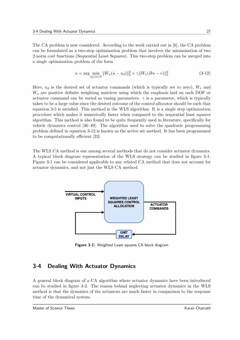
The WLS CA method is one among several methods that do not consider actuator dynamics.A typical block diagram representation of the WLS strategy can be studied in figure 3-1.Figure 3-1 can be considered applicable to any related CA method that does not account foractuator dynamics, and not just the WLS CA method.
Figure 3-1: Weighted Least squares CA block diagram
3-4 Dealing With Actuator Dynamics
A general block diagram of a CA algorithm where actuator dynamics have been introducedcan be studied in figure 3-2. The reason behind neglecting actuator dynamics in the WLSmethod is that the dynamics of the actuators are much faster in comparison to the responsetime of the dynamical system.
Master of Science Thesis Karan Chatrath

28 Control Allocation Theory
Figure 3-2: Control allocation with actuator dynamics considered
The WLS method can indeed operate effectively when actuators respond fast. However, whenthe dynamics of the actuators are relatively slower, the WLS loses effectiveness. Since manyCA methods lack the ability to handle actuator dynamics, alternate approaches that over-come this shortcoming become necessary. The subsequent section goes into details of onesuch method.
3-5 Model Predictive Control Allocation
MPCA is a control allocation technique based on model predictive control and it effectivelyaccounts for the actuator dynamics. This section of the chapter is dedicated to the theoryof MPCA. Model predictive control is an optimal control technique based on the idea ofreceding horizon control. The theory behind MPC is developed in detail in [5]. The followingparagraphs briefly explain how MPC works.
The controller can be formed based on a linear or nonlinear model of the plant. This math-ematical model of the plant is used to look ahead in time and understand how the plant isexpected to evolve with time. This mathematical description is also known as the predictionmodel and the time duration for which it looks ahead is known as the prediction horizon.
After having computed the prediction model and predicted the future throughout the pre-diction horizon, a set of control inputs are computed for a certain number of time steps intothe future. This number of time steps is known as the control horizon. This computation iscarried out by solving an optimization problem. This optimization problem reflects certaincontrol objectives and is usually convex in nature. MPC allows the designer to account forconstraints on the inputs and outputs. After having solved the optimization problem, fromthe resulting set of control inputs that span the control horizon, only the first element of thecontrol input vector is applied to the plant. This process is repeated for each time step asthe plant’s behaviour evolves.
Karan Chatrath Master of Science Thesis

3-5 Model Predictive Control Allocation 29
MPCA works in a similar fashion, except here, the dynamics behaviour captured is that ofthe actuators. The theory of MPCA has been developed based on [50] and [5]. The rest ofthis section is dedicated to the formulation of the MPCA problem. Consider the followingsystems of actuators of an over actuated mechanical system. The number of actuators isconsidered to be Nu, and each actuator is modelled as a continuous-time, linear dynamicalsystem. The dynamics of the i-th actuator is of the form
xi(t) = Aixi(t) +Biuci(t− δi)ui = Cixi
(3-13)
Here, xi represents the states of the i-th actuator, uci represents the command sent to thei-th actuator, and ui is the response of the i-th actuator. Here, i ∈ (1, 2, 3 . . . Nu). Sincethe MPCA algorithm operates in discrete time, each of these actuators can be discretizedaccording to the zero-order hold (ZOH) operation. The resulting discrete-time dynamics ofeach actuator, without any loss of generality, can be represented as
xi (k + 1) = Adixi (k) +Bdiuci(k)ui(k) = Cdixi(k)
(3-14)
The actuator dynamics can be combined into a single state-space description as suchx1(k + 1)x2(k + 1)
...xNu(k + 1)
=
Ad1 0 . . . 00 Ad2 . . . 0...
... . . . 00 0 . . . AdNu
x1(k)x2(k)
...xNu(k)
+
Bd1 . . . 0... . . . ...0 . . . BdNu
uc1(k + 1)uc2(k + 1)
...ucNu(k + 1)
u1(k)u2(k)
...uNu(k)
=
Cd1 0 . . . 00 Cd2 . . . 0...
... . . . 00 0 . . . CdNu
x1(k)x2(k)
...xNu(k)
(3-15)
Equations 3-15 can be written in short as
x (k + 1) = Adx (k) +Bduc (k)u (k) = Cndx(k)
(3-16)
Equation set 3-16 describes the combined discrete-time actuator dynamics. Recall that v =Bu. Using this, the following is obtained
x (k + 1) = Adx (k) +Bduc (k)u (k) = Cndx(k)BCnd = Cd
(3-17)
Master of Science Thesis Karan Chatrath

30 Control Allocation Theory
Finally, the combined state-space representation of the actuator dynamics is
x (k + 1) = Adx (k) +Bduc (k)v(k) = Cdx(k)
(3-18)
The sizes of each system matrix is: Ad ∈ IRNs×Ns ,Bd ∈ IRNs×Nu , Cd ∈ IRNo×Ns . Forformulating the MPCA problem, the notation shown above will be used consistently. Tobegin the formulation of the problem, three key pieces of information are necessary. Thesampling time of the control system, the prediction horizon Np and the control horizon Nc.Knowing this, the equation 3-19 can be iterated for future time steps as shown
v (k + 1) = CdAdx (k) + CdBd uc (k)v (k + 2) = CdA
2dx (k) + CdAdBd uc (k) + CdBd uc(k + 1)
...v (k +Np) = CdA
Npd + CdA
Np−1d Bd uc (k) + · · ·+ CdA
Np−Ncd Bd uc (k +Nc − 1)
(3-19)
This set of iterated equations can be combined in a matrix form as suchv(k + 1)v(k + 2)
...v(k +Np)
=
CdAdCdA
2d
...CdA
Npd
x (k) +
CdBd . . . 0No×NuCdAdBd . . . 0No×Nu
... . . ....
CdANp−1d Bd . . . CdA
Np−Ncd Bd
uc(k)uc(k + 1)
...uc(k +Nc − 1)
(3-20)
Here, the notation 0p×q represents a matrix of p rows and q columns and having all elementsas zero. The equation 3-20 can be rewritten in a condensed form
V (k) = Fx (k) + φ Uc(k) (3-21)
Equation 3-21 is known as the predictor model based on which the controller operates. Thematrix F is of a similar form as the observability matrix and the matrix φ is known asthe Toeplitz matrix. The sizes of each of these matrices and vectors are V (k) ∈ IRNpNo×1,F ∈ IRNpNo×Ns , φ ∈ IRNpNo×NuNc and Uc(k) ∈ IRNuNc×1. The next step in the formulation ofthe MPCA problem is accounting for constraints imposed on the actuators. Recall that theconstraints on the actuators comprise of position as well as rate limits. The rate constraintscan be re-written as position constraints as in equation 3-11. The vector variable in theMPCA optimization problem is the vector Uc. The constraints need to be recast in termsof that. All the actuator commands computed through MPCA must satisfy all constraintsthroughout the control horizon Nc. This is done as such
Ain =[−INu×Nc INu×Nc
]TbL =
[uc uc . . . uc
]TbU =
[uc uc . . . uc
]Tbin =
[−bL bU
]T(3-22)
Karan Chatrath Master of Science Thesis

3-6 A Simple Example 31
The relations in equation 3-22 can be combined to yield a combined set of inequality con-straints
AinUc ≤ bin (3-23)
Having computed the predictor model, as per equation 3-22 and the constraints on the MPCAproblem as per equation 3-23, the next step is to define the control allocator objective. Letus consider a high-level controller to be generating a virtual input vector or control demandnamely vref . The control allocator must compute a set of actuator commands such that theactuators together produce this control demand throughout the prediction horizon. This canbe captured by doing the following. The reference virtual control demand is defined referredto as Vref .
Vref =[vref vref . . . vref
]T(3-24)
Here, Vref ∈ IRNpNo×1. Now, the MPCA optimization is formulated as such. It is formedsuch that it is a convex optimization problem. The cost function is defined as
J = (V (k)− Vref )T W (V (k)− Vref ) + Uc (k)T Q Uc(k) (3-25)
The objective is to minimise the cost function J with respect to the vector Uc such thatthe constraints defined in equation 3-23 are satisfied. Equation 3-21 is replaced in the costfunction and expanded leading to the formation of a convex quadratic programming problem.This concludes the formulation of the MPCA problem. The MPCA problem has several tun-ing parameters. There is the sample time of the control allocator T and the prediction andcontrol horizons and the diagonal elements of the weighting matrices W and Q.
3-6 A Simple Example
In this section, a simple example is presented to the readers. This example is aimed atdemonstrating certain features and possible shortcomings. of the CA algorithms used in thisthesis. A system comprising of two actuators is considered as such:
u1 = −2u1 + 2u1c
u2 = −u2 + u2c
(3-26)
The position and rate limits of each actuator are taken to be the same in this example. Theposition is limited between −20 ≤ ui ≤ 20. The rate is limited between −500 ≤ ui ≤ 500.Here i ∈ {1, 2}. The scenario here is that the system is equipped with a high-level controllerand a control allocator. The hypothetical high-level controller works such that it produces atime-varying virtual control demand v which is of the form
v = 10 sin(t) (3-27)
The system is over actuated since a single control demand v has to be optimally distributedamong two actuators. Here, the control effectiveness matrix is taken as
B = [1 2] (3-28)
Master of Science Thesis Karan Chatrath

32 Control Allocation Theory
At first, the weighted Least squares control allocator is tested on this system without con-sidering actuator dynamics according to figure 3-1. The tuning parameters for the controlallocator are as per table 3-1.
Tuning Parameter ValueControl Allocation Effectiveness weight - Wv 1
Actuator Command Weight - Wu diag[0.1;0.1]Relative Weight - γ 1
Sampling Time of CA 0.01 secMax. Number of Iterations 100
Table 3-1: Simple Example - WLS - CA Tuning Parameters
The control allocator, in this case, works effectively as can be seen in figure 3-3. The effec-tiveness of the control allocator is assessed by how well the actuators can together producethe required demand. In other words how close is Bu to v.
Figure 3-3: Simple example - WLS - CA - No actuator Dynamics
Without actuator dynamics considered, the control allocator works effectively as seen inthe figure above. On the introduction of actuator dynamics (according to figure 3-2), theeffectiveness of the control allocator can be assessed in figure 3-4. In this case, the controlallocator’s tuning parameters are kept the same as the previous case where actuator dynamicswere not considered. It can be seen that the introduction of actuator dynamics causes adeterioration in the effectiveness of the control allocator. This is because the WLS methodneglects actuator dynamics.
Karan Chatrath Master of Science Thesis

3-6 A Simple Example 33
Figure 3-4: Simple example - WLS - CA - With actuator Dynamics
The next step of this simple example is to test the model predictive control allocation algo-rithm. Keeping in mind that the system is equipped with actuators described in equations3-26, the tuning parameters for the MPCA algorithm can be studied in table 3-2.
Figure 3-5: Simple example - MPCA
In table 3-2, the weight matrices W and Q need to be resized according to the predictionand control horizons. The effectiveness of the MPCA method can be assessed in figure 3-5. Figure 3-5 demonstrates that MPCA can handle actuator dynamics. However, MPCAoperates under one assumption. The assumption is that the actuator dynamics are knownand that there are no large uncertainties in the actuator dynamics.
Master of Science Thesis Karan Chatrath

34 Control Allocation Theory
Tuning Parameter ValueControl Allocation Effectiveness Weight - W 1
Actuator Commands Weight - Q diag([0.01;0.01])Prediction Horizon - Np 50Control Horizon - Nc 20Sampling Time of CA 0.01 sec
Table 3-2: Simple Example - MPCA Tuning Parameters
3-7 MPCA With Adaptive Parameter Estimation (APE)
It was mentioned that the MPCA algorithm operates under the assumption that the actuatordynamics are known. This section tests a situation where this is not the case. This test wascarried out by operating under the premise that the MPCA algorithm is formulated based onthe set of actuator dynamics described as
u1 = −20u1 + 20u1c
u2 = −70u2 + 70u2c
(3-29)
The actual actuator parameters are according to those described in equations 3-26. All tuningparameters are according to table 3-2. In figure 3-6, it is seen that there is a reduction in theeffectiveness of the control allocator. The actuators do manage to meet the demand v butthis happens after a visible delay. This shortcoming of handling actuator uncertainties willbe addressed in this section by combining the MPCA algorithm with a parameter estimatorwhich is adaptive in nature.
Figure 3-6: Simple example - MPCA with actuator uncertainties
Karan Chatrath Master of Science Thesis

3-7 MPCA With Adaptive Parameter Estimation (APE) 35
3-7-1 Online adaptive parameter estimation
The work carried out in the area of system identification and parameter estimation has beenof great interest in the past decades and continues to be a topic that researchers embarkon. In this thesis, the parameter estimation algorithm used is the Auxiliary Model BasedRecursive Least Squares (AM-RLS) Algorithm. Details of this work can be found in [51,52].The algorithm is described in this section. Consider a general discrete-time transfer functiondescribing some form of input-output relationship of the form
Y (z)U(z) = 1
zd
(a0z
m + a1zm−1 + a2z
m−2 + · · ·+ amzn + b1zn−1 + b2zn−2 + · · ·+ bn
)(3-30)
Here, d is a known delay and the variables m and n are also known. The coefficients of eachpower of the variable z are considered unknown. This transfer function can be re-written assuch: (
zn + b1zn−1 + b2z
n−2 + · · ·+ bn)Y (z) =(
a0zm−d + a1z
m−1−d + a2zm−2−d + · · ·+ a−d
m
)U(z)
(3-31)
Now, both sides are multiplied by a filter of the form 1/(z + λ)n to give(zn
(z + λ)n + b1zn−1
(z + λ)n + b2zn−2
(z + λ)n + · · ·+ bn1
(z + λ)n)Y (z) =(
a0zm−d
(z + λ)n + a1zm−1−d
(z + λ)n + a2zm−2−d
(z + λ)n + · · ·+ amz−d
(z + λ)n)U(z)
(3-32)
Now, taking the inverse Z-transform on both sides yields filtered versions of the signals y(k)and u(k). The filtered versions of the signals obey the following notation
Z−1[zn−iY (z)(z + λ)n
]= yfi(k)
Z−1[zm−d−iU(z)
(z + λ)n]
= ufi(k)
(3-33)
Here, λ is a number which is chosen by the user and its magnitude is taken to be within theunit circle centered at the origin. With this in mind equation 3-31 is converted into timedomain giving the following
yf0(k) + b1yf1(k) + b2yf2(k) + · · ·+ bnyfn(k) = a0uf0(k) + a1uf1(k) + a2uf2(k)+· · ·+ amufm(k)
(3-34)
After a bit of rearrangement
z(k) = φT (k)θ(k)
φ(k) =[−yf1(k) . . . −yfn(k) uf0(k)(k) . . . ufm(k)
]Tθ(k) =
[b1 b2 . . . bn a0 a1 . . . am
]T(3-35)
Master of Science Thesis Karan Chatrath

36 Control Allocation Theory
The above equation 3-35 is referred to as a linear-in-the-parameters parametric model. Here,z(k) is the signal yf0(k), which, like φ(k), is also computed at each instant of time. It isbased on this parametric model that parameter estimation is carried out. The estimate ofthe parameter vector at the present time instant is referred to as θ(k). Having explained theparametric model, the AM-RLS algorithm is presented as follows [51,52]
θ(k) = θ(k − 1) + P (k)φ(k)(z(k)− φT (k)θ(k − 1)
)P (k) = P (k − 1) + P (k − 1)φ(k)φT (k)P (k − 1)
1 + φT (k)P (k − 1)φ(k)(3-36)
The initial conditions of the algorithm can be defined by setting P (0) to be a larger numberlike 100 or 1000, and the initial parameter estimate θ(0) can be set to smaller values (0.1, 0.01,etc.). There are a number of parameter estimation methods that exist in literature that makeuse of the parametric model in 3-35. Typically, such estimators are derived by minimizingsome kind of a cost function. What distinguishes different algorithms is the structure ofthe cost function and the resulting speed of parameter convergence of the algorithm. TheAM-RLS algorithm, just like many others operates under a few assumptions. They are:
• Only the input and output of the system to be estimated are measured and all mea-surements are noise-free.
• The order of the system, number of zeros and the input delay of the system are consid-ered to be known quantities.
• The input to the system is persistently exciting. It is this condition which is necessaryand sufficient to ensure asymptotic convergence of parameters.
This adaptive parameter estimation algorithm is henceforth abbreviated as ’APE’ for therest of this report. This parameter estimator is combined with the MPCA algorithm. Thiscombination is henceforth referred to as ’APE+MPCA’ or ’APE with MPCA’.
3-7-2 Combining APE with MPCA
The APE algorithm fits input-output data to transfer functions with a known structure anddelay. In the event where the actuator dynamics to be considered in MPCA are uncer-tain, it can be combined with the APE to overcome this uncertainty. This combination ofAPE+MPCA is tested on the simple example described earlier. In this case, all tuning pa-rameters of the MPCA are defined according to table 3-2. Additionally, the initial values ofthe matrix P and the vector θ are set to 100I2 where I2 is the identity matrix of size 2, and[0.1 0.1
]Trespectively. The effectiveness of this control allocation algorithm can be assessed
in figure 3-7. It is seen that the shortcoming of handling actuator uncertainties is effectivelyhandled by the MPCA algorithm combined with the parameter estimator.
The parameter convergence can be studied in figure 3-8. The reader is asked to observethe values to which the parameters converge. If one were to take the dynamics defined in
Karan Chatrath Master of Science Thesis

3-7 MPCA With Adaptive Parameter Estimation (APE) 37
equation 3-26, and perform a zero-order hold discretization with a sampling time of 0.01s,the parameters of the resulting first-order discrete transfer functions would be the same asthe ones seen in figure 3-8.
Figure 3-7: Simple example - APE with MPCA
Figure 3-8: Simple example - APE with MPCA - Parameter Convergence
Master of Science Thesis Karan Chatrath

38 Control Allocation Theory
3-8 Summary
This chapter laid out the underlying theory of control allocation. The problem was formu-lated and a brief review of literature was carried out. Among all methods briefly discussed,the weighted least squares algorithm was elaborated in detail and its shortcomings were high-lighted. Keeping the shortcomings in mind, the theory of model predictive control allocationwas developed. Both these methods were tested on a simple example based on which each oftheir features and shortcomings was demonstrated. After establishing that MPCA is not aseffective when actuator dynamic uncertainties are present, the MPCA algorithm is combinedwith an adaptive parameter estimator.
These three approaches of control allocation, namely, weighted least squares, MPCA andAPE+MPCA is what this entire thesis is based on. Using these allocation strategies, vehi-cle yaw rate stability control systems are designed and evaluated on simulation. A detailedanalysis of these control systems is the subject of the subsequent chapters of this report.
Karan Chatrath Master of Science Thesis

Chapter 4
Electronic Stability Control UsingControl Allocation
This chapter delves into the domain of vehicle dynamics control. All the theory built up in theprevious chapters leads to this application. The vehicle is stabilised by controlling its yaw rate,using differential braking or active steering or a combination of both. A basic introduction tovehicle stability control is given in the introductory chapter of this thesis. This chapter, onthe other hand, goes into the details and results of the work carried out. Vehicle dynamicscontrol has been covered in several publications. A lot of the theory applied in this thesisis inspired by literature. Noteworthy references are that of Laine [46–49] and Shyrokau [53,54].
While assessing the controllers designed in this chapter on simulation, the vehicle is subjectedto the standard ISO Sine With Dwell test (refer section 2-6). Before going into the details ofthe control system design, a need for vehicle yaw rate control is established in the followingsection.
4-1 Sine With Dwell Test With No Control
In this section, the performance of the vehicle, with no stability controller, when subjectedto the Sine With Dwell (SWD) Test is studied, using IPG CarMaker. The SWD test is per-formed by varying the steering wheel angle amplitudes (SWA) for a given initial vehicle speedof 80 km/hr. The vehicle performance can be studied in figure 4-1.
It can be seen that the vehicle loses stability beyond 110 degrees of SWA. There is a consid-erable loss of vehicle speed and the yaw rate does not stabilize to zero after completion of thesteering input. It can also be seen that the vehicle experiences high lateral accelerations ofnearly 0.8 g’s. Such levels of accelerations indicate that the vehicle is operating near its limits
Master of Science Thesis Karan Chatrath

40 Electronic Stability Control Using Control Allocation
of handling. An aggressive steering input of 115 degrees SWA causes the vehicle to spin outof control.
Figure 4-1: Vehicle Response With No Control
The necessity to control the stability of the vehicle is therefore established. Loss of lateralcontrol also manifests itself in the form of high body slip angles. This quantity indicates thatthe vehicle acquires high lateral velocity which needs to be regulated appropriately. The workconducted in this thesis is, however, confined to yaw rate control.
4-2 General Layout Of The Stability Control System
This section aims to give a brief layout of the control system. A general block diagram of theclosed-loop system can be studied in figure 4-2. It can be seen that the plant model is thevehicle model within IPG CarMaker. The goal is to control the Yaw rate of the plant model.The overall control system has been divided into three subsystems which are: the referencegenerator, the high-level controller and the control allocation algorithm.
The goal of the reference generator is to generate a signal that represents the desired yawrate that the vehicle must acquire. The high-level controller performs the computation of acorrective yaw moment in the event where it detects a difference between actual and desiredyaw rates of the vehicle. The control allocation algorithm has the task of distributing the highlevel control action among available actuators in such a way that the response of the actuatorswhen combined amounts to the corrective yaw moment demanded by the high level controller.
Karan Chatrath Master of Science Thesis

4-3 Reference Generator 41
Figure 4-2: General Block Diagram for ESC Using Control Allocation
Subsequent sections of this report will elaborate on each of these subsystems in detail.
4-3 Reference Generator
The yaw rate to be controlled requires a desired signal to which the controller drives it. Thereference yaw rate can be obtained in more than one way. In this report, two approaches arereported. One approach is shown as follows and is based on the linear bicycle model.
x = Ax+Bδδ
x =[vy ψ
]T(4-1)
The linear bicycle model is a highly simplified 2-DOF vehicle model described in equation4-1. The system matrices are shown in chapter 2, equation 2-23. The reference signal can begenerated based on this model. However, since the model is simplified, the peak reference yawrate computed by the linear bicycle model does not account for the limitations of the roadconditions. The coefficient of friction must be factored into this calculation and the upperand lower bound of the yaw rate is
ψbound =∣∣∣∣µgvx
∣∣∣∣ (4-2)
Here, µ is the friction coefficient and vx is the longitudinal velocity of the vehicle. Thissequence of computations based on the linear bicycle model does limit the yaw rate. However,the resulting reference signal has some ’abrupt changes’ or ’sharp corners’. This can have anadverse impact on passenger comfort as the control system tends to follow this ’desired’ signaland abrupt changes can lead to higher jerk. To avoid this, another approach is used whichgenerates a smooth curve as the reference yaw rate signal. This second approach also involvesthe use of the bicycle model, however, in this case, only its steady-state response is considered.
Master of Science Thesis Karan Chatrath

42 Electronic Stability Control Using Control Allocation
Looking at equation 4-1, one can compute the steady-state yaw rates and lateral velocitiesby equating its derivatives to zero as such
xss =[vyss ψss
]T= −A−1Bδδ (4-3)
The steady-state yaw rate expression is then limited according to equation 4-2. This isthen filtered through a standard second-order transfer function of appropriate frequency anddamping. This filter is designed so that the filtered steady state yaw rate response is as closeas possible to that of the linear bicycle model. The reference trajectories predicted by bothapproaches can be seen in figure 4-3. These reference signals in figure 4-3 are generated forthe sine with dwell test. The signals will be different for different manoeuvres are they dependon the driver steering input.
Figure 4-3: Reference signals for yaw rate control for the sine with dwell test
The natural frequency and damping ratio of this second-order filter is ωn = 15 rad/sec andζ = 0.7. It can seen in figure 4-3 that the steady-state filtered response is much smootherthan that predicted by the linear bicycle model.
Karan Chatrath Master of Science Thesis

4-4 High-Level Controller 43
4-4 High-Level Controller
It was explained in previous chapters that by using control allocation, the task of controlsystem design can be separated into sub-tasks. One is the high-level control while the otheris the control allocation algorithm. The high-level controller is independent of any details ofthe actuators and is therefore independent of the control allocation algorithm. Consider theequations of motion of a planar vehicle as described in equation 2-4. This is rewritten hereas such
m 0 00 m 00 0 Izz
vxvyψ
=
mψvy−mψvx
0
+
FxFyMz
(4-4)
This can be wriiten as
Mx = f(x) + v (4-5)
Equation 4-5 is clearly devoid of any actuator commands. The task of the high-level controlleris to compute the vector v of corrective forces and moments. In this thesis, different controlallocation algorithms are used. However, the high-level controller parameters in all thesecases are kept constant (irrespective of the number of actuators used and control allocationalgorithm applied) in order to compare the results objectively. Note that
v =[Fx Fy Mz
]T(4-6)
Since the control objective is that of yaw rate, the high-level controller computes a correctiveyaw moment for the vehicle. In other words
v =[0 0 Mz,corr
]T(4-7)
The high-level controller is kept as simple as necessary. The term f(x) in equation 4-5 isneglected during control for this reason. The choice of the controller is a standard discrete-time proportional-derivative regulator operating at 100 Hz. The proportional controller ismeant to drive the yaw rate response towards the reference signal while the derivative actionis used to ensure that the response is adequately damped. Tuning of this controller was doneby trial and error and its form is:
C(z) = Kp +KdN
1 + NTsz−1
(4-8)
The error signal is defined as e(k) and its Z transform is denoted by E(z)
e(k) = ψref (k)− ψ(k) (4-9)
Master of Science Thesis Karan Chatrath

44 Electronic Stability Control Using Control Allocation
Here ψref (k) and ψ(k) are discrete-time yaw rate signals sampled at 100 Hz. k is the presenttime instant. The corrective yaw moment is computed as follows:
Mz,corr(k) = Z−1 [C(z)E(z)] (4-10)
The high-level control action is therefore v(k) =[0 0 Mz,corr(k)
]T. The controller tuning
parameters are kept constant for all simulations reported for vehicle stability control analysis.They are summarised in table 4-1. These parameters were obtained after tuning the closed-loop control system depicted in figure 4-2.
Tuning Parameter ValueProportional Control - Kp 9000Derivative Control - Kd 1000Filter Coefficient - N 1
Table 4-1: High Level PD Controller as in equation 4-6 - Tuning parameters
The controller has been tuned so that the vehicle can be stabilized up to a steering wheel am-plitude of 130 degrees. This is a limited range of operation, however, the objective remainsto evaluate the control allocation strategies as opposed to controlling the vehicle for moreaggressive steering inputs. Even in the range where the SWA is between 110 degrees and 115degrees, the vehicle experiences high lateral accelerations and a considerable amount of bodyslip (figure 4-1). Controlling the vehicle, albeit in this limited range, is of great importance.
4-5 Control Effectiveness Matrix Derivation
Recall that in previous chapters, it was mentioned that in order to use a control allocationalgorithm, a mapping between states to be controlled and actuator commands is necessary.Such a mapping is often linear and of the form described in equation v = Bu. B is the controleffectiveness matrix. This section derives the mapping between planar motion and availableactuators. Consider the planar vehicle model described in section 2-2. If one were to neglectthe effect of steering angles in the equations of motion (described in equations 2-5, 2-6, 2-7)by approximating sin (δ) = 0,cos (δ) = 1, they simplify to.
Fx = Fxrl + Fxrr + Fxfl + Fxfr
Fy = Fyrl + Fyrr + Fyfl + Fyfr
Mz = (Fyfl + Fyfr)Lf − (Fyrl + Fyrr)Lr + Tf2 (−Fxfl + Fxfr) + Tr
2 (−Fxrl + Fxrr)
(4-11)
Consider the single corner model as described in equation 2-9. If one were to neglect thewheel angular accelerations, the model gets reduced to a steady-state relationship which is
Fxi = Tdi − Tbirw
(4-12)
Karan Chatrath Master of Science Thesis

4-5 Control Effectiveness Matrix Derivation 45
Equation 4-12 can be replaced in equation set 4-11. Additionally, the linear tire model(section 2-3-1) can be used to replace the lateral forces. The small-angle approximation isapplied to the slip angle equations. The resulting equation is what is finally used to establisha relationship between the forces/moments and actuator commands. Equation set 4-11 canbe written generally as
v = h (x, u) (4-13)
Where x is a state vector and u is the actuator command vector. The following cases are nowconsidered.
4-5-1 Case 1: 4 Actuators - Differential Braking
The number of high level control actions is three and the number of available actuators isfour. In other words, v =
[Fx Fy Mz
]Tand u =
[Tbfl Tbfr Tbrl Tbrr
]T.
Using 4-13, one can obtain the control effectiveness for this case by carrying out the followingoperation
B = ∂h
∂u(4-14)
This gives the mapping v = Bu, which is
FxFyMz
=
−1rw
− 1rw
− 1rw
− 1rw
0 0 0 0Tf2rw − Tf
2rwTr
2rw − Tr2rw
TbflTbfrTbrlTbrr
(4-15)
4-5-2 Case 2: 5 Actuators - Differential Braking And Active Front Steering
The number of high level control actions is three and the number of available actuators is five.In other words, v =
[Fx Fy Mz
]Tand u =
[Tbfl Tbfr Tbrl Tbrr δ
]T. By carrying out
the same steps as done in the previous case, one can obtain the required mapping v = Bu,where is control effectiveness matrix is:
B =
−1rw
− 1rw
− 1rw
− 1rw
00 0 0 0 CαfTf2rw − Tf
2rwTr
2rw − Tr2rw CαfLf
(4-16)
Here, Cαf = Cαfl + Cαfr is the front axle cornering stiffness of the vehicle. This mappingdeveloped (in each case) between states and actuator commands is essential for the controlallocation as will be seen in subsequent sections.
Master of Science Thesis Karan Chatrath

46 Electronic Stability Control Using Control Allocation
4-6 Summary Of All Simulation Scenarios
The signals generated by the high-level controller, or the virtual input, or the control demand,are fed into the control allocation algorithm. The task of the control allocation algorithm isthe coordination of available actuators such that the control demand is met. In the processof carrying out yaw rate control by employing control allocation methods, several scenarioswith different algorithms have been evaluated on simulation. This section aims to clearlypresent all the scenarios considered. The simulations have been carried out by increasing thecomplexity of the control allocation algorithm in a progressive manner. As mentioned earlier,two actuator configurations have been considered. One configuration uses four actuators(Differential braking) while the other uses braking and active front steering.
4-6-1 Configuration 1: With Four Actuators
The control effectiveness matrix for this actuator configuration is presented in equation 4-15.The following scenarios are assessed.
• Case A: Weighted Least squares with no actuator dynamics
• Case B: Weighted least squares algorithm with simplified brake actuator dynamics
• Case C: MPCA with simplified brake actuator dynamics
• Case D: MPCA with simplified brake actuator dynamics and with actuator uncertainties
• Case E: APE+MPCA with simplified brake actuator dynamics
4-6-2 Configuration 2: With Five Actuators
The control effectiveness matrix for this actuator configuration is presented in equation 4-16.The following scenarios are assessed.
• Case F: Weighted Least squares with no actuator dynamics
• Case G: Weighted least squares algorithm with simplified brake and steering actuatordynamics
• Case H: MPCA with simplified brake and steering actuator dynamics
• Case I: MPCA with simplified brake and steering actuator dynamics and with actuatorparameter uncertainties
Karan Chatrath Master of Science Thesis

4-7 Details Of Simulation Scenarios and Results 47
4-6-3 Additional Scenarios
It can be seen that from cases A to I, only simplified actuator dynamics are used for investi-gations. The following scenarios incorporate either the Hybdrulic brake model as describedin section 2-5-1 or the Pfeffer Steering model as described section 2-5-2. Additionally, somepractical constraints and considerations from a vehicle dynamics standpoint are consideredfor some cases. The practical considerations include the following:
• Incorporation of the limits of tire force generation in the control allocation constraints.
• Modifying the control effectiveness matrix so as to make it dynamic in nature.
The additional cases considered are:
• Case J: APE+MPCA using five actuators. Here the brake dynamics are simple as persection 2-5-1. However, the steering model in use is the relatively complex Pfeffer Model(see section 2-5-2).
• Case K: APE+MPCA using five actuators. Here the brake dynamics are simple as persection 2-5-1. However, the steering model in use is the Pfeffer Model. The limits ontire force generation and the dynamic control effectiveness matrix are also incorporatedin this analysis.
• Case L: WLS using four actuators. In this scenario, the hydraulic brake model is usedinstead of the simplified brake actuator dynamics. The limits on tire force generationand the dynamic control effectiveness matrix are also incorporated in this analysis.
• Case M: APE+MPCA using four actuators. In this scenario, the hydraulic brake modelis used instead of the simplified brake actuator dynamics. The limits on tire forcegeneration and the dynamic control effectiveness matrix are also incorporated in thisanalysis.
The scenario of using five actuators, all of which are not described by simplified dynamicswas attempted, however, the simulations crashed. In all, there are 13 scenarios which havebeen named as Cases A to M. Each of these scenarios are discussed in subsequent sections.Most of the simulation results are presented in appendix B. It should be noted that the highlevel PD controller has the same set of tuning parameters in all cases listed above.
4-7 Details Of Simulation Scenarios and Results
The underlying theory behind control allocation has been discussed in chapter 3 in detail.Specifically, the weighted least squares algorithm and the model predictive control allocationalgorithm were described. Combining the MPCA algorithm with an adaptive parameter esti-mation technique was also elaborated upon. These techniques are all used for vehicle stabilitycontrol.
Master of Science Thesis Karan Chatrath

48 Electronic Stability Control Using Control Allocation
Recall that in chapter 2, two actuator configurations were defined. One configuration com-prises of four actuators (brakes only) while the other is a combination of brakes with activefront steer. The control effectiveness matrices for each of these cases have been derived andare found in equations 4-15 and 4-16. For most of the simulations carried out, the simplifieddynamics of the brake and steering actuators were used as described in 2-5. The limits of thebrake actuators are defined as follows
uMax = 1800 NmuMin = 0 NmρMax = 12000 Nm/secρMin = −8000 Nm/secuMin ≤ uc(t) ≤ uMax
ρMin ≤ uc(t) ≤ ρMax
(4-17)
The steering system dynamics is described using a second-order transfer function describedin section 2-5-2. The limits of the active front steering steering actuation are
uMax,AFS = 30◦
uMin,AFS = −30◦ Nm
ρMax,AFS = 50◦/sec
ρMin,AFS = −50◦/sec
uMin,AFS ≤ uc(t) ≤ uMax,AFS
ρMin,AFS ≤ uc(t) ≤ ρMax,AFS
(4-18)
4-7-1 Tuning Parameters
The tuning parameters for the WLS - CA algorithm can be studied in table 4-2. The generalblock diagram for WLS CA can be seen in figure 3-1.
Tuning Parameter ValueControl Allocation Effectiveness weight - Wv diag[0;0;1]
Actuator Command Weight - Wu diag[0.1;0.1;0.1;0.1]Relative Weight - γ 1
Sampling Time of CA 0.01 secMax. Number of Iterations 100
Table 4-2: Tuning Parameters - 4 Actuators - WLS - CA
The reason for choosing Wv to be larger than Wu is because a greater emphasis needs tobe placed on reference tracking than limiting the magnitude of actuator commands. γ istypically chosen to be very high values like 106. However, here, a nominal value is chosen asa larger value may result in unnecessarily high brake torques, in the process of minimising
Karan Chatrath Master of Science Thesis

4-7 Details Of Simulation Scenarios and Results 49
the error between v and Bu. The sample time of the control allocator is kept similar tothat of the high-level controller. A lower sampling time would result in many more instanceswhere the optimization problem needs to be solved. This would lead to an increase in onlinecomputational load. The tuning parameters for the MPCA algorithm can be seen in table4-3.
Tuning Parameter ValueControl Allocation Effectiveness Weight - W diag[0;0;1]
Actuator Commands Weight - Q diag([0.1;0.1;0.1;0.1])Prediction Horizon - Np 30Control Horizon - Nc 10Sampling Time of CA 0.01 sec
Table 4-3: Tuning Parameters - 4 Actuators - MPCA - Simple brake actuator
Figure 4-4: MPCA BLOCK Diagram - General
The weight matrices W and Q need to be resized according to the prediction and controlhorizons. Lower sampling time of a model predictive control allocator enables it to effectivelyreject unknown disturbances [55]. On the other hand, a low sampling time for the CA alsoincreases the computational load. In the simulations reported, the selected scenarios are de-void of unknown disturbances, so the sampling time is taken to be the same as that of thehigh-level controller.
A rule of thumb for the choice of prediction horizon is that it should be chosen so that itcan look ahead throughout the transient response of the slowest actuator [55]. This was con-sidered while tuning the controllers. The control horizon should ideally be kept as low aspossible. This is because the number of variables for the optimization problem reduces, thuspromoting faster computations and convergence. However, small values like Nc = 2 do notenable the system to respond in the desired way. The control horizon was increased up to apoint where the response of the vehicle and the control allocator is considered acceptable. Ageneral block diagram for the MPCA algorithm can be seen in figure 4-4.
Master of Science Thesis Karan Chatrath

50 Electronic Stability Control Using Control Allocation
The third control allocation technique involves the combination of APE and MPCA. The tun-ing parameters of the MPCA solver are kept the same as table 4-3. The parameter estimator,in this case, works on estimating two unknown parameters of a first-order transfer functionwith a known time delay. The APE algorithm requires initialization of two quantities as perequation 3-36. One initialization is that of the initial estimate of the unknown parametervector θ(0) while the other is the matrix P (0). The initial conditions for the APE can beseen in the following table.
Tuning Parameter Valueθ(0) [0.1;0.1]P(0) 100I2
Table 4-4: APE Initialization - 4 Actuators - APE + MPCA - Simple brake actuator
Figure 4-5: APE+MPCA BLOCK Diagram - General
It should be noted that in table 4-4, the symbol I2 denotes the identity matrix of size two. Ageneral block diagram where APE is combined with MPCA can be studied in figure 4-5. Ithas been described earlier that the APE requires knowledge of the order of the system, thedelay, and the input and output of the dynamics to be estimated. The estimated parametersare then fed back into the MPCA algorithm following which the control allocation problemis solved with the knowledge of the estimated actuator dynamics.
The tuning parameters defined in tables 4-2, 4-3, 4-4 are mainly defined for the four actuatorconfiguration. The following tables show the tuning parameters when five actuators are inuse. The tuning parameters for the WLS algorithm can be seen in table 4-5.
Karan Chatrath Master of Science Thesis

4-7 Details Of Simulation Scenarios and Results 51
Tuning Parameter ValueControl Allocation Effectiveness weight - Wv diag[0;0;1]
Actuator Command Weight - Wu diag[0.1;0.1;0.1;0.1;5000]Relative Weight - γ 1
Sampling Time of CA 0.01 secMax. Number of Iterations 100
Table 4-5: Tuning Parameters - 5 Actuators - WLS - CA
The tuning parameters for MPCA can be studied in table 4-6. The prediction and controlhorizons are chosen according to the description given earlier in this section. A very largeweight is placed on the AFS action. The reason behind doing so is the same as that donewhile using the WLS algorithm.
Tuning Parameter ValueControl Allocation Effectiveness weight - W diag[0;0;1]
Actuator Command Weight - Q diag([0.1;0.1;0.1;0.1;108])Prediction Horizon - Np 30Control Horizon - Nc 25Sampling Time of CA 10−2 sec
Table 4-6: Tuning Parameters - 5 Actuators - MPCA - simple brake and steering actuators
The block diagrams for the MPCA and APE+MPCA strategies can be seen in figures 4-4and 4-5 respectively.
4-7-2 Simulation Scenario Case E
Most of the results obtained for each scenario as described in section 4-6 are reported inappendix B. In this section, case E is discussed. Recall that case E is the scenario wherefour simplified brake actuators are considered. The control allocation algorithm used is theAPEMPCA technique.
Figure 4-6, shows the performance of the vehicle in the sine with dwell test for a given steeringwheel angle amplitude (SWA). It is seen that the vehicle is stabilized for SWA up to 130degrees. Figure 4-7 shows the corresponding brake torques generated by the ESC controller.Figure 4-8 gives an idea of the performance metrics of the sine with dwell test, as described insection 2-6. The idea here is that if the yaw rate or the lateral displacement curves intersectwith the red dashed lines, then the manoeuvre fails. It can be seen in figure 4-8 that thevehicle behaves in a stable manner for a steering input of 130 degrees amplitude.
Master of Science Thesis Karan Chatrath
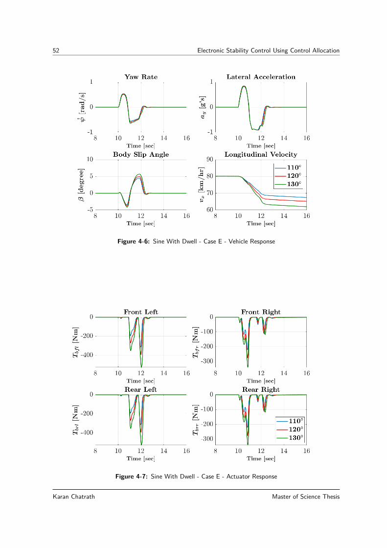
52 Electronic Stability Control Using Control Allocation
Figure 4-6: Sine With Dwell - Case E - Vehicle Response
Figure 4-7: Sine With Dwell - Case E - Actuator Response
Karan Chatrath Master of Science Thesis

4-7 Details Of Simulation Scenarios and Results 53
Figure 4-8: Sine With Dwell - Case E - SWA - 130 degrees
The control allocation algorithm works effectively in this scenario. The parameter estimationconvergence and the control allocation effectiveness can be studied in appendix B.
4-7-3 Simulation Scenario - Case J
This section aims to address cases J as defined in section 4-6. The results in the cases Ato I only consider simplified actuator dynamics. The simplified actuator dynamics are lineardynamical systems. It has been seen that the MPCA algorithm when combined with theAPE works effectively. Estimating the parameters of a linear system of a known order andstructure is a manageable task. However, in reality, things are different. The mathematicalstructure of the dynamics of the actuators is usually unknown. In fact, the governing dynam-ics of the actuators could be highly nonlinear. In this case, an attempt has been made to ’fit’the response of an unknown actuator to a linear dynamical system.
Looking at the scenario defined in case J, the goal of this investigation is to see whether theresponse of the steering system can be fit into a linear dynamical system. More specifically,can the steering response be fit into a first order transfer function? The simulations thatfollow make use of the tuning parameters described in table 4-7. Recall that the high-levelcontroller is kept constant throughout all cases.
The input to the steering system is the driver input (steering wheel angle) + AFS and theoutput is the road wheel angle δ. The parameter estimator uses this input-output informationto fit the response to a first order transfer function.
Master of Science Thesis Karan Chatrath

54 Electronic Stability Control Using Control Allocation
Tuning Parameter ValueControl Allocation Effectiveness Weight - W diag[0;0;1]
Actuator Command Weight - Q diag([0.1;0.1;0.1;0.1;106])Prediction Horizon - Np 30Control Horizon - Nc 25Sampling Time of CA 10−2 secAPE parameter: P(0) 10I2APE parameter: θ(0) [0.1 ; 0.1]
Table 4-7: Tuning Parameters - 5 Actuators - APE+MPCA - Simple Brake Model + NonlinearSteering Dynamics
The results of the simulations carried out for the case J is summarized in Appendix B. How-ever, an important observation is highlighted. When the active front steer is combined withdifferential braking, the total control demand is distributed among a larger number of actu-ators. As a result, the magnitudes of brake torques generated by the controller are lower. Aconsequence of this is that the vehicle experiences a lower loss of speed as opposed to whenonly four actuators are used. One can argue based on this that integrated yaw rate controlusing brakes and active front steering is a better option for vehicle dynamics control.
Another observation to be noted is that despite the response of the steering system beingapproximated by a first-order transfer function, the control allocation algorithm still workseffectively. The subsequent sections delve into the incorporation of practical considerationsfrom a vehicle dynamics standpoint following which cases K and M are discussed.
4-8 Additional Vehicle Dynamics Factors
In the previous section, a part of the simulation scenarios (as described in section 4-6) isdiscussed. It was reported that APE combined with MPCA effectively handles actuator dy-namics as well as actuator uncertainties. However, those evaluations carried out were stilltheoretical in nature. Practical aspects from a vehicle dynamics standpoint need to be takeninto consideration.
One such practical consideration is the pneumatic tires. Tires, in general, are limited in theirperformance. No tire can produce an unlimited amount of force. So while the control alloca-tion algorithm does consider the limits of the actuators, it also needs to take into considerationthe limits of the tire. To elaborate a bit further, the brake system aids in the generation ofa braking torque in the wheels. This, in turn, results in the generation of longitudinal tireforces that cause the vehicle to decelerate. During an aggressive manoeuvre, a situation mayarise where the tire cannot produce the force required to decelerate the vehicle. This couldresult in a loss of traction with the road, which can be dangerous. Therefore, it is imperativeto factor in the limits of the tire in the constraints of the control allocation problem.
The second practical consideration is the variation of cornering stiffness during a manoeuvre.The cornering stiffness of a tire is usually considered constant at low slip angles. However,
Karan Chatrath Master of Science Thesis

4-8 Additional Vehicle Dynamics Factors 55
the tire characteristics indicate that this is not the case for higher slip angles. Taking thisvariation into account results in the control effectiveness matrix becoming dynamic in nature(see equation 4-16). Each of these practical considerations is addressed as follows.
4-8-1 Tire Limits As Control Allocation Constraints
Here, the Dugoff tire model is considered. According to the equations laid out in section2-3-2, the lateral force developed in each tire can be estimated. This lateral force can then beused to compute the maximum possible longitudinal force that the tire can develop. This isdone using the concept of the friction circle (equation 2-17). Having computed the maximumpossible longitudinal force that can be developed, the limiting brake torque can be found bymultiplying that force with the effective radius of the wheel.
Fx,max =√(
µFz)2 − (Fy)2 (4-19)
Tmax = Fx,maxrw (4-20)
The following few equations have been highlighted in chapter 3, they are however redescribedhere for the sake of completeness. Looking back at the constraints on the brake actuators forthe CA problem, we have
uMin ≤ u(t) ≤ uMax (4-21)
ρMin ≤ u(t) ≤ ρMax (4-22)
The rate limits can be re written as position limits by approximating the derivative as follows.
u (t) ≈ u (t)− u(t− T )T
(4-23)
Based on the actuator limits, the constraints are
ulower ≤ u ≤ uupper (4-24)
Where
ulower = max[uMin, u (t− T ) + TρMin]uupper = min[uMax, u (t− T ) + TρMax]
(4-25)
By incorporating the limits of longitudinal tire force generation (equation 4-20), the overallconstraints are
u ≤ u ≤ u (4-26)
Where,
u = ulower
u = min(uupper, Tmax)(4-27)
Master of Science Thesis Karan Chatrath

56 Electronic Stability Control Using Control Allocation
4-8-2 Variation of Cornering Stiffness
The cornering stiffness of a tire is typically defined for a linear tire model as in equation2-16. This quantity is taken as a constant assuming that the tire operates in a range of verysmall slip angles. However, the need for stability control arises when the vehicle is pushedto its limits of handling. The assumption of small slip angles in that region is not a suitableone. Moreover, using a linear tire model for investigations of such nonlinear manoeuvres isan oversimplification of the scenario. To understand the nature of variation of tire corneringstiffness, a case presented in the previous section is revisited. Specifically, case J (section 4-6)is looked at. In this simulation scenario, an extra step was carried out, which had no impacton the results of the simulation. This extra step involved understanding the variation ofcornering stiffness as the manoeuvre progresses with time. Using the Dugoff model equation2-18, we have
Fyi = Cαi tanαi1− κi
f (λ) (4-28)
By assuming, small angles, one can write tan(α) = α. Dividing both sides by α leads toan expression Fy/α on the left-hand side of equation 4-28. This can be thought of as thecornering stiffness which varies with time and other tire-related quantities.
Each tire has a cornering stiffness associated with it. However, from a vehicle dynamicsstandpoint, it is useful to know the combined front cornering stiffness (used in the controleffectiveness matrix). A plot of this time-varying front cornering stiffness can be studied infigure 4-9.
Figure 4-9 shows that the variation in the quantity is high and that treating it as a constantis not suitable. Based on this assessment, it was decided to dynamically update the frontcornering stiffness in the control effectiveness matrix B. Upon inspecting the control effec-tiveness matrix a bit further, it was seen that the matrix has a few elements which are zero.This matrix has been shown in equation 4-29 again.
It was demonstrated earlier that the static control effectiveness matrix was derived by assum-ing small angles in the planar model. In this section, this assumption no longer holds true.The control effectiveness matrix is now derived using the planar model making a fewer num-ber of approximations. The linear tire model is still in use, however, the cornering stiffness isupdated according to the Dugoff model, as described earlier.
B =
−1rw
− 1rw
− 1rw
− 1rw
00 0 0 0 CαfTf2rw − Tf
2rwTr
2rw − Tr2rw CαfLf
(4-29)
This modification of the control effectiveness is inspired by the work carried out by Shyrokau[53]. The expression for the control effectiveness matrix is described in equation 4-30. Thisexpression for the control effectiveness described in equation 4-30, the terms Cαfl and Cαfrare the front left and front right cornering stiffness values computed using the Dugoff tiremodel as described earlier.
Karan Chatrath Master of Science Thesis

4-8 Additional Vehicle Dynamics Factors 57
8 9 10 11 12 13 14 15 16
0.4
0.6
0.8
1
1.2
1.4
1.610
5
Figure 4-9: Variation of Cornering stiffness with time during the sine with dwell manoeuvre
Bbrakes =
− cos(δ)/rw − cos(δ)/rw −1/rw −1/rw− sin(δ)/rw − sin(δ)/rw 0 0
Tf cos(δ)−2Lf sin(δ)rw
−Tf cos(δ)−2Lf sin(δ)rw
Tr2rw − Tr
2rw
BAFS =
−(Cαfl + Cαfl) sin(δ)(Cαfl + Cαfl) cos(δ)
(Cαfl + Cαfl) cos(δ) + (Cαfl−Cαfl)Tf sin(δ)2
B =
[Bbrakes BAFS
](4-30)
Master of Science Thesis Karan Chatrath

58 Electronic Stability Control Using Control Allocation
4-9 Simulations Scenarios: Cases K and M
Simulation Scenarios Cases K,L and M (section 4-6) take into consideration the vehicle dy-namics effects discussed in section 4-8. The APE+MPCA algorithm for this situation has ablock diagram as described in figure 4-10.
Figure 4-10: APE with MPCA accounting for tire limits and dynamic control effectiveness
Figure 4-11: Sine With Dwell Test - Case K - Vehicle Response
Karan Chatrath Master of Science Thesis

4-9 Simulations Scenarios: Cases K and M 59
Figure 4-12: Sine With Dwell Test - Case K - Actuator Response
With this understanding, the simulation for scenario Case K was carried out and the resultsare presented in the figures 4-11 and 4-12.
Figure 4-12 can be compared with figure 4-7. It was mentioned earlier that integrated controlresults in lower brake torques being generated when compared to the use of only differentialbraking. This results in a lower loss of speed. It is seen that for a steering wheel angle am-plitude of 130 degrees, the vehicle speed reduces to approximately 62 km/hr when only fouractuators are used, while the speed reduces to 65 km/hr when five actuators are used. Thiscomparison can be done by looking at figures 4-11 and 4-6. The greater loss of speed whenonly using differential braking is probably insignificant to a driver. However, a larger loss ofspeed is expected in more aggressive manoeuvres, where higher brake torques are likely tobe generated by the controller. The inference from this comparison is that integrated controlis a better alternative to differential braking since it has a lower impact on other states ofmotion like longitudinal velocity.
The tuning parameters are as described in table 4-7. The difference between cases J and Kis that case K incorporates tire limits and a dynamic control effectiveness matrix while caseJ does not. The results demonstrate that the vehicle is stabilised and the control allocationstrategy is effective. Additional results for case K can be studied in Appendix B. A comparisonfor the results of cases J and K was carried out to see the benefit of incorporating additionalvehicle dynamics factors. This comparison can be seen in figure 4-13. It can be seen thatthe yaw rate response is marginally better in case K as the vehicle stabilises faster than in
Master of Science Thesis Karan Chatrath

60 Electronic Stability Control Using Control Allocation
case J. Also, the amount of body slip experienced by the vehicle in case K is lower. Thisis desirable since the vehicle experiences a lesser amount of unwanted lateral motion, or ’drift’.
Figure 4-13: Sine With Dwell Test - Case J and K Comparison - Vehicle Response - SWA - 130degrees - Case J: Static B, Case K: Dyn B
4-9-1 Simulations With Hydraulic Brake Model
All simulations reported until case K consider simplified first-order brake actuator dynamics(section 2-5-1). However, to perform a more realistic assessment of the control system, thesimple brake model has been replaced by a hydraulically actuated brake (HAB) model asdescribed in section 2-5-1. This section reports observations made while simulating case M(refer section 4-6).
The control allocation technique in use in case M is APE+MPCA. An attempt is madeto fit the response of the HAB actuator to a linear dynamical system. More specifically, afirst-order transfer function. The results of case M can be studied in the following figures. Inthis case, only a SWA amplitude of 115 degrees is simulated. Simulations for more aggressivemanoeuvres fail due to numerical issues.
It can be seen in figure 4-16 that the SWD test nearly fails. Moreover, in figure 4-14 it can beseen that the vehicle experiences body slip angles greater than 10 degrees and a comparativelygreater loss of speed as it drops below 60 km/hr. Furthermore, the brake torques generatedby the controller are of a very ’jerky’ nature as seen in figure 4-15. This kind of brake systemresponse can cause passenger discomfort. Looking at the control allocation effectiveness infigure 4-17, it can be seen that the effectiveness considerably reduces.
Karan Chatrath Master of Science Thesis

4-9 Simulations Scenarios: Cases K and M 61
Figure 4-14: Sine With Dwell Test - Case M - Vehicle Response
Figure 4-15: Sine With Dwell Test - Case M - Vehicle Response
Master of Science Thesis Karan Chatrath

62 Electronic Stability Control Using Control Allocation
Figure 4-16: Sine With Dwell Test - Case M - SWA - 115 degrees
8 9 10 11 12 13 14 15 16
-2
-1
0
1
2
3
4
5
6
Figure 4-17: Sine With Dwell Test - Case M - Control Allocation Effectiveness
This kind of result can be explained primarily by the nature of the hydraulic brake system inuse. Referring to section 2-5-1, one can see that the HAB system is equipped with two setsof valves, each of which operates independently of each other. One set of valves is responsiblefor brake pressure build-up while the other regulates pressure release. On noticing figure 4-15,one can see that the rate at which pressure builds up is not the same as the rate at which it is
Karan Chatrath Master of Science Thesis

4-10 Summary 63
released. Different rates of increase and decrease cannot be fit into a linear first-order dynamicsystem which was the attempt made in case M. The nature of the HAB system dynamics isin fact, quite different from that predicted by a first-order transfer function. Approximatingbrake dynamics as a first order system has been carried out by [12]. In conclusion, byusing simplified brake actuator dynamics, the APE+MPCA control allocation method showspromising results. However, the introduction of a complex HAB system renders the controlallocation method to be ineffective.
4-10 Summary
In this chapter, the details of the ESC system design were presented. This was followed byan assessment of 13 simulation scenarios starting named as case A to M (refer section 4-6).Certain key results have been presented in this chapter while most of the results are presentedin appendix B. It was observed that the APE+MPCA control allocation technique was ef-fective when the brake actuator dynamics were described by a first-order transfer function.Moreover, it was observed that the response of the Pfeffer Steering model can be fit to afirst-order transfer function and doing so resulted in no loss of control allocation effectiveness.On introducing the more realistic HAB actuator model, it was seen that the APE+MPCAtechnique loses effectiveness. The response of the brake system cannot be fitted to a first-order linear system since the rate at which brake pressures (or torque) builds up and the rateat which the system releases pressure is different. Modelling such a system requires a moredetailed and possibly non-linear mathematical description.
Master of Science Thesis Karan Chatrath

64 Electronic Stability Control Using Control Allocation
Karan Chatrath Master of Science Thesis
Chapter 5
Conclusions And Recommendations
5-1 Highlights And Conclusions
The primary goal of this thesis was to investigate the concept of control allocation and applythe technique for vehicle stability control. It was found that the Control Allocation (CA)strategy enables optimal distribution of high-level control commands among available actua-tors. Furthermore, CA can perform such an optimal distribution by accounting for the limitsof the actuators.
To accomplish the design of electronic stability control systems using control allocation, twoactuator configurations were of focus. One configuration comprised of four actuators (differ-ential braking) while the second comprised of five actuators (Differential braking and activefront steering). For each of these actuator configurations, the Weighted Least Squares (WLS)CA method was at first applied without considering actuator dynamics. The results obtainedfor each of these cases demonstrated the benefit of coordinating a larger number of actuators.The high-level yaw moment correction when distributed among a larger number of actuatorsresulted in the generation of lower brake torques by the control system. This, in turn, resultedin a lower unwanted loss of speed at the end of the sine with dwell manoeuvre. In conclusion,the use of integrated control results in lower actuator commands and better vehicle perfor-mance.
Upon the introduction of actuator dynamics (governed by transfer functions), a deteriorationof the effectiveness of the WLS method was visible. This deterioration manifests itself in twoways. The actuators fail to meet the demand generated by the high-level controller and theclosed-loop system performance deteriorates. The need to account for actuator dynamics wasestablished and this warranted the use of Model Predictive Control Allocation (MPCA). Itwas seen that the MPCA method overcomes the shortcomings of the WLS and other suchmethods that do not consider actuator dynamics.
Master of Science Thesis Karan Chatrath

66 Conclusions And Recommendations
This work also drew attention to the fact that MPCA loses effectiveness when uncertaintiesin actuator dynamics are present. This was addressed by combining the MPC allocator alongwith an adaptive parameter estimator. It was shown that the APE+MPCA control allocationtechnique successfully handles actuator uncertainties when the actuators obey linear dynam-ics.
In reality, actuator responses are more complex than what simple linear dynamics can predict.With this understanding, keeping the brake actuators simple, the linear steering actuator dy-namic system was replaced with a more detailed Pfeffer Steering Model. An attempt wasmade to fit the response of the steering system to a linear dynamical system by using input-output data. The results demonstrated that the APE+MPCA strategy performs effectivelydespite the introduction of a complex steering model.
Finally, the linear brake system actuators were replaced with a detailed Hydraulic brakemodel. Upon attempting to fit the response of the brake system to a linear dynamic system,it was seen that the APE+MPCA strategy loses effectiveness. The reason for this result isthat the brake system comprises two sets of valves that operate independently. This resultedin rates of brake pressure build-up and release to be different. Such behaviour cannot bemodelled or fit as a linear dynamic system. It can be concluded that simplified actuatormodels for brakes inadequately capture hydraulic brake system behaviour.
In conclusion, the APE+MPCA control allocation technique can effectively deal with actuatoruncertainties as long as the actuators are governed by uncertain linear dynamics. The methodalso shows promise in some situations where the actuators in use are unknown and nonlinear.In this case, the CA solver successfully handles complex steering dynamics effectively. TheAPE+MPCA technique loses effectiveness when actuator behaviours are too complex to befit to a linear dynamical system.
5-2 Recommendations And Scope For Future Work
The author draws attention to the first sentence of the first chapter of this report. ’Ad-vancement is a continuous process’. The scope for improvement in any field is never-ending.Recognizing and acting on this scope is the key to advancement. The field of vehicle dynam-ics control is no exception to this fact. Automotive companies’ research and developmentactivities are constantly working towards the betterment of Advanced Driver Assistance Sys-tems (ADAS) and automated driving. Considering all the work carried out in this thesis, thefollowing recommendations are made:
• The high-level controller used in this thesis is a simple discrete-time PD controller. Thishas a limited range of operation as seen in the simulations. The vehicle, for most cases,could not be controlled for more aggressive sine with dwell manoeuvres (>130 degreesof SWA). Use of techniques such as feedback linearization or even high-level nonlinear
Karan Chatrath Master of Science Thesis

5-2 Recommendations And Scope For Future Work 67
model predictive control could prove to be a better choice than a simple PD compen-sator.
• In the APE+MPCA strategy, the adaptive parameter estimator is independent of theMPCA solver. In this case, only the identified parameters are fed into the MPCA solver.The parameter estimation technique used in this work is the AM - RLS technique whichoperates under the assumptions that the order and structure of the dynamical systemis known and is linear, the input delay (if any) is also a known quantity. The AM-RLStechnique can be easily replaced with a parameter estimator that makes fewer assump-tions. It is possible that the linear MPCA solver combined with a better parameterestimator can result in more effective control allocation.
• The actuator dynamics used for the most part of this thesis are linear in nature. It wasdemonstrated that by simulating the control system with more realistic brake actuatordescriptions, the control allocation effectiveness reduces. It is therefore highly recom-mended to carry out investigations with realistic actuator descriptions as opposed tousing simplified models. If the governing dynamics of the actuators become nonlinear,then the MPCA solver would also be of a nonlinear nature. The use of nonlinear MPCAis expected to handle nonlinear actuator dynamics effectively. Also, actuator aging canbe a potential problem. Nonlinear MPCA combined with nonlinear parameter estima-tors can result in fault-tolerant control allocation.
• From a vehicle dynamics standpoint, the controlled vehicle has been subjected to thestandard ISO sine with dwell test. The controller can be evaluated in different manoeu-vres in both simulations as well as real-time testing. More specifically, scenarios, wherethe vehicle is subjected to unknown disturbances, low friction conditions, poor roadconditions must be looked into to assess the robustness of the overall control system.
Master of Science Thesis Karan Chatrath

68 Conclusions And Recommendations
Karan Chatrath Master of Science Thesis
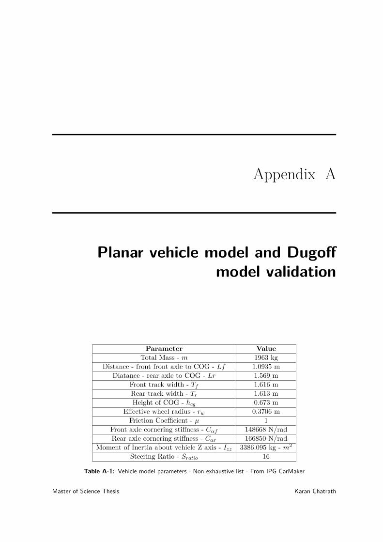
Appendix A
Planar vehicle model and Dugoffmodel validation
Parameter ValueTotal Mass - m 1963 kg
Distance - front front axle to COG - Lf 1.0935 mDiatance - rear axle to COG - Lr 1.569 m
Front track width - Tf 1.616 mRear track width - Tr 1.613 mHeight of COG - hcg 0.673 m
Effective wheel radius - rw 0.3706 mFriction Coefficient - µ 1
Front axle cornering stiffness - Cαf 148668 N/radRear axle cornering stiffness - Cαr 166850 N/rad
Moment of Inertia about vehicle Z axis - Izz 3386.095 kg - m2
Steering Ratio - Sratio 16
Table A-1: Vehicle model parameters - Non exhaustive list - From IPG CarMaker
Master of Science Thesis Karan Chatrath

70 Planar vehicle model and Dugoff model validation
Figure A-1: Validation with Steering wheel angle amplitude of 100 degrees
Figure A-2: Validation with Steering wheel angle amplitude of 110 degrees
Karan Chatrath Master of Science Thesis

71
Figure A-3: Validation with Steering wheel angle amplitude of 130 degrees
Figure A-4: Dugoff Tire Model Validation - SWA - 130 degrees - TM (Tire Model)
Master of Science Thesis Karan Chatrath

72 Planar vehicle model and Dugoff model validation
Karan Chatrath Master of Science Thesis

Appendix B
ESC with Control Allocation - Results
The specifics of each following case can be found in section 4-6.
B-1 Case A Results
Figure B-1: Sine With Dwell - Case A - Vehicle Response
Master of Science Thesis Karan Chatrath

74 ESC with Control Allocation - Results
Figure B-2: Sine With Dwell - Case A - Actuator Response - Brake Torques
Figure B-3: Sine With Dwell - Case A - SWA - 130 degrees
Karan Chatrath Master of Science Thesis

B-2 Case B Results 75
8 9 10 11 12 13 14 15 16
-2
-1.5
-1
-0.5
0
0.5
1
1.5
2
2.5
Figure B-4: Sine With Dwell - Case A - SWA - 130 degrees - Control Allocation Effectiveness
B-2 Case B Results
Figure B-5: Sine With Dwell - Case A and B comparison - Vehicle Response Legend: NoDyn -Case A, ActDyn - Case B
Master of Science Thesis Karan Chatrath

76 ESC with Control Allocation - Results
Figure B-6: Sine With Dwell - Case A and B comparison - Actuator Response - Brake Torques- Legend: NoDyn - Case A, ActDyn - Case B
Figure B-7: Sine With Dwell - Case B - SWA - 130 degrees
Karan Chatrath Master of Science Thesis

B-3 Case C Results 77
8 9 10 11 12 13 14 15 16
-2
-1
0
1
2
3
4
Figure B-8: Sine With Dwell - Case B - SWA - 130 degrees - Control Allocation Effectiveness
B-3 Case C Results
Figure B-9: Sine With Dwell - Case C - Vehicle Response
Master of Science Thesis Karan Chatrath

78 ESC with Control Allocation - Results
Figure B-10: Sine With Dwell - Case C - Actuator Response - Brake Torques
Figure B-11: Sine With Dwell - Case C - SWA - 130 degrees
Karan Chatrath Master of Science Thesis

B-4 Case D Results 79
8 9 10 11 12 13 14 15 16
-2
-1.5
-1
-0.5
0
0.5
1
1.5
2
2.5
Figure B-12: Sine With Dwell - Case C - SWA - 130 degrees - Control Allocation Effectiveness
B-4 Case D Results
8 9 10 11 12 13 14 15 16
-2
-1.5
-1
-0.5
0
0.5
1
1.5
2
2.5
Figure B-13: Sine With Dwell - Case D - SWA - 130 degrees - Control Allocation Effectiveness
Master of Science Thesis Karan Chatrath

80 ESC with Control Allocation - Results
Figure B-14: Sine With Dwell - Case D - SWA - 130 degrees
B-5 Case E Results
8 9 10 11 12 13 14 15 16
-1.5
-1
-0.5
0
0.5
1
1.5
2
2.5
Figure B-15: Sine With Dwell - Case E - SWA - 130 degrees - Control Allocation Effectiveness
Karan Chatrath Master of Science Thesis

B-6 Case F Results 81
Figure B-16: Sine With Dwell - Case E - SWA - 130 degrees - Brake Actuators’ parameterestimation convergence
B-6 Case F Results
Figure B-17: Sine With Dwell - Case F - Vehicle Response
Master of Science Thesis Karan Chatrath

82 ESC with Control Allocation - Results
Figure B-18: Sine With Dwell - Case F - Actuator Response
Figure B-19: Sine With Dwell - Case F - SWA - 130 degrees
Karan Chatrath Master of Science Thesis

B-7 Case G Results 83
8 9 10 11 12 13 14 15 16
-2
-1
0
1
2
3
4
Figure B-20: Sine With Dwell - Case F - SWA - 130 degrees - Control Allocation Effectiveness
B-7 Case G Results
Figure B-21: Sine With Dwell - Case F and G comparison - Vehicle Response - Legend: NoDyn- Case F, ActDyn - Case G
Master of Science Thesis Karan Chatrath

84 ESC with Control Allocation - Results
Figure B-22: Sine With Dwell - Case F and G comparison - Actuator Response - Legend: NoDyn- Case F, ActDyn - Case G
Figure B-23: Sine With Dwell - Case G - SWA - 130 degrees
Karan Chatrath Master of Science Thesis

B-8 Case H Results 85
8 9 10 11 12 13 14
-4
-2
0
2
4
6
8
Figure B-24: Sine With Dwell - Case G - SWA - 130 degrees - Control Allocation Effectiveness
B-8 Case H Results
Figure B-25: Sine With Dwell - Case H - Vehicle Response
Master of Science Thesis Karan Chatrath

86 ESC with Control Allocation - Results
Figure B-26: Sine With Dwell - Case H - Actuator Response
Figure B-27: Sine With Dwell - Case H - SWA - 130 degrees
Karan Chatrath Master of Science Thesis

B-9 Case I Results 87
8 9 10 11 12 13 14 15 16
-4
-3
-2
-1
0
1
2
3
4
5
Figure B-28: Sine With Dwell - Case H - SWA - 130 degrees - Control Allocation Effectiveness
B-9 Case I Results
8 9 10 11 12 13 14 15 16
-2
-1
0
1
2
3
4
Figure B-29: Sine With Dwell - Case I - SWA - 130 degrees - Control Allocation Effectiveness
Master of Science Thesis Karan Chatrath

88 ESC with Control Allocation - Results
Figure B-30: Sine With Dwell - Case I - SWA - 130 degrees
B-10 Case J Results
Figure B-31: Sine With Dwell - Case J - Vehicle Response
Karan Chatrath Master of Science Thesis

B-10 Case J Results 89
Figure B-32: Sine With Dwell - Case J - Actuator Response - Brake Torques
Figure B-33: Sine With Dwell - Case J - SWA - 130 degrees
Master of Science Thesis Karan Chatrath

90 ESC with Control Allocation - Results
8 9 10 11 12 13 14 15 16
-2
-1.5
-1
-0.5
0
0.5
1
1.5
2
2.5
3
Figure B-34: Sine With Dwell - Case J - SWA - 130 degrees - Control Allocation Effectiveness
Figure B-35: Sine With Dwell - Case J - Brake Actuator Parameter Estimation
Karan Chatrath Master of Science Thesis

B-11 Case K Results 91
0 5 10 15
0
0.02
0.04
0.06
0.08
0.1
0.12
0.14
0.16
0.18
8 10 12 14 16
-8
-6
-4
-2
0
2
4
6
8
10
Figure B-36: Sine With Dwell - Case J - Pfeffer Steering Actuator Parameter Estimation
B-11 Case K Results
Figure B-37: Sine With Dwell - Case K - SWA - 130 degrees
Master of Science Thesis Karan Chatrath

92 ESC with Control Allocation - Results
8 9 10 11 12 13 14 15 16
-1.5
-1
-0.5
0
0.5
1
1.5
2
2.5
Figure B-38: Sine With Dwell - Case K - SWA - 130 degrees - Control Allocation Effectiveness
Figure B-39: Sine With Dwell - Case K - Brake Actuator Parameter Estimation
Karan Chatrath Master of Science Thesis

B-12 Case L Results 93
0 5 10 15
0
0.02
0.04
0.06
0.08
0.1
0.12
0.14
0.16
0.18
8 10 12 14 16
-8
-6
-4
-2
0
2
4
6
8
10
Figure B-40: Sine With Dwell - Case K - Pfeffer Steering Actuator Parameter Estimation
B-12 Case L Results
Figure B-41: Sine With Dwell - Case L - Vehicle Response
Master of Science Thesis Karan Chatrath

94 ESC with Control Allocation - Results
Figure B-42: Sine With Dwell - Case L - Actuator Response - Brake Torques
Figure B-43: Sine With Dwell - Case L - SWA - 130 degrees
Karan Chatrath Master of Science Thesis

B-13 Case M Results 95
8 9 10 11 12 13 14 15 16
-2
-1
0
1
2
3
4
5
Figure B-44: Sine With Dwell - Case L - SWA - 130 degrees - Control Allocation Effectiveness
B-13 Case M Results
Figure B-45: Sine With Dwell - Case M - Brake Actuator Parameter Estimation - SWA - 115degrees
Master of Science Thesis Karan Chatrath

96 ESC with Control Allocation - Results
Karan Chatrath Master of Science Thesis
Bibliography
[1] SAE On-road Automated Vehicles Standards Committee and others, “SAE J3016: Tax-onomy and Definitions for Terms Related to On-Road Motor Vehicle Automated DrivingSystems,” SAE J3016, Sep, 2016.
[2] R. Rajamani, Vehicle Dynamics And Control. Springer, 2011.
[3] T. A. Johansen and T. I. Fossen, “Control Allocation-A Survey,” Automatica, vol. 49,no. 5, pp. 1087–1103, 2013.
[4] B. De Schutter and T. J. van den Boom, “Optimization In Systems and Control-LectureNotes-Department Of Systems and Control-Delft University Of Technology,”
[5] L. Wang, Model predictive control system design and implementation using MATLAB R©.Springer Science & Business Media, 2009.
[6] O. Härkegård, Backstepping and Control Allocation with Applications to Flight Control.PhD thesis, Linköpings universitet, 2003.
[7] “CarMaker | IPG Automotive.” https://ipg-automotive.com/products-services/simulation-software/carmaker/. Accessed: 2019-06-21.
[8] IPG CarMaker Reference Manual. IPG Automotive.
[9] R. N. Jazar, Vehicle dynamics: theory and application. Springer, 2017.
[10] S. M. Savaresi and M. Tanelli, Active braking control systems design for vehicles. SpringerScience & Business Media, 2010.
[11] H. Dugoff, P. Fancher, and L. Segel, “An analysis of tire traction properties and theirinfluence on vehicle dynamic performance,” SAE transactions, pp. 1219–1243, 1970.
[12] J. Zhou, J. Lu, and H. Peng, “Vehicle stabilization in response to exogenous impulsivedisturbances to the vehicle body,” in 2009 American Control Conference, pp. 701–706,IEEE, 2009.
Master of Science Thesis Karan Chatrath

98 Bibliography
[13] R. Mousseau, D. Song, B. Miller, G. Semrau, T. Klingler, and D. Jones, “Using Simu-lation to Quantify Sine with Dwell Maneuver Test Metric Variability,” tech. rep., SAETechnical Paper, 2008.
[14] S. M. Arndt, M. W. Arndt, and M. Rosenfield, “Effectiveness of Electronic StabilityControl on Maintaining Yaw Stability when an SUV has a Rear Tire Tread Separation,”SAE International Journal of Passenger Cars-Electronic and Electrical Systems, vol. 2,no. 2009-01-0436, pp. 120–140, 2009.
[15] N. Picot, B. Miller, M. D. Rizzo, and T. A. Klingler, “FMVSS126 Electronic StabilityControl Sine with Dwell Incomplete Vehicle Type 2 Analysis,” SAE International Journalof Passenger Cars-Mechanical Systems, vol. 4, no. 2011-01-0956, pp. 713–721, 2011.
[16] M. Bodson, “Evaluation of Optimization Methods for Control Allocation,” Journal ofGuidance, Control, and Dynamics, vol. 25, no. 4, pp. 703–711, 2002.
[17] M. W. Oppenheimer, D. B. Doman, and M. A. Bolender, “Control Allocation for Over-Actuated Systems,” in Control and Automation, 2006. MED’06. 14th MediterraneanConference on, pp. 1–6, IEEE, 2006.
[18] K. A. Bordingnon and W. C. Durham, “Closed-form Solutions to Constrained Con-trol Allocation Problem,” Journal of Guidance, Control, and Dynamics, vol. 18, no. 5,pp. 1000–1007, 1995.
[19] W. C. Durham, “Constrained Control Allocation-Three-Moment Problem,” Journal ofGuidance, Control, and Dynamics, vol. 17, no. 2, pp. 330–336, 1994.
[20] W. C. Durham, “Attainable Moments For The Constrained Control Allocation Problem,”Journal of Guidance, Control, and Dynamics, vol. 17, no. 6, pp. 1371–1373, 1994.
[21] W. Durham, K. A. Bordignon, and R. Beck, Aircraft Control Allocation. John Wiley &Sons, 2017.
[22] K. A. Bordignon, Constrained Control Allocation For Systems With Redundant ControlEffectors. PhD thesis, Virginia Tech, 1996.
[23] O. Harkegard, “Efficient Active Set Algorithms for Solving Constrained Least SquaresProblems in Aircraft Control Allocation,” in Decision and Control, 2002, Proceedings ofthe 41st IEEE Conference on, vol. 2, pp. 1295–1300, IEEE, 2002.
[24] E. Lundsager Hansen and C. Völcker, “Numerical Algorithms for Sequential QuadraticOptimization,” Master’s thesis, Technical University of Denmark, DTU, DK-2800 Kgs.Lyngby, Denmark, 2007.
[25] P. Hungerländer, “Algorithms for Convex Quadratic Programming,” 2014.
[26] O. Härkegård, “Quadratic Programming Control Allocation Toolbox QCAT For MAT-LAB,” 2004.
[27] M. L. Glaze, The Design and Implementation of a GUI-Based Control Allocation Toolboxin the MATLAB Environment. PhD thesis, Virginia Tech, 1998.
Karan Chatrath Master of Science Thesis

99
[28] J. Pei, G. Bassett, J. Grisham, P. Finch, M. Toniolo, L. Miller, , and P. Bandu, “GenericControl Allocation Toolbox for Preliminary Vehicle Design,” in Modeling and SimulationTechnologies Conference, 2018.
[29] O. Härkegård and S. T. Glad, “Resolving Actuator RedundancyâĂŤOptimal Control vs.Control Allocation,” Automatica, vol. 41, no. 1, pp. 137–144, 2005.
[30] J. B. Davidson, F. J. Lallman, and W. T. Bundick, “Real-Time Adaptive Control Allo-cation Applied to a High Performance Aircraft,” 2001.
[31] A. Cristofaro and T. A. Johansen, “Fault Tolerant Control Allocation Using UnknownInput Observers,” Automatica, vol. 50, no. 7, pp. 1891–1897, 2014.
[32] H. Ríos, S. Kamal, L. M. Fridman, and A. Zolghadri, “Fault Tolerant Control Alloca-tion via Continuous Integral Sliding-Modes: a HOSM-Observer Approach,” Automatica,vol. 51, pp. 318–325, 2015.
[33] Y. Liu and L. G. Crespo, “Adaptive Control Allocation in the Presence of ActuatorFailures,” Journal of Control Science and Engineering, vol. 2012, p. 3, 2012.
[34] A. Casavola and E. Garone, “Enhancing the Actuator Fault Tolerance in AutonomousOveractuated Vehicles via Adaptive Control Allocation,” in Mechatronics and Its Appli-cations, 2008. ISMA 2008. 5th International Symposium on, pp. 1–6, IEEE, 2008.
[35] A. Casavola and E. Garone, “Fault-Tolerant Adaptive Control Allocation Schemes forOveractuated Systems,” International Journal of Robust and Nonlinear Control, vol. 20,no. 17, pp. 1958–1980, 2010.
[36] F. Liao, K.-Y. Lum, J. Wang, and M. Benosman, “Adaptive Control Allocation for Non-linear Systems with Internal Dynamics,” IET control theory & applications, vol. 4, no. 6,pp. 909–922, 2010.
[37] A. Khelassi, J. Jiang, D. Theilliol, P. Weber, and Y. Zhang, “Reconfiguration of ControlInputs for Overactuated Systems Based on Actuators Health,” in Proceedings of 18thIFAC World Congress, 2011.
[38] P. Weber, B. Boussaid, A. Khelassi, D. Theilliol, and C. Aubrun, “Reconfigurable Con-trol Design with Integration of a Reference Governor and Reliability Indicators,” Interna-tional Journal of Applied Mathematics and Computer Science, vol. 22, no. 1, pp. 139–148,2012.
[39] M. A. Bolender and D. B. Doman, “Nonlinear Control Allocation Using Piecewise LinearFunctions,” Journal of Guidance, Control, and Dynamics, vol. 27, no. 6, pp. 1017–1027,2004.
[40] V. L. Poonamallee, S. Yurkovich, A. Serrani, and D. B. Doman, “A Nonlinear Pro-gramming Approach for Control Allocation,” in American Control Conference, 2004.Proceedings of the 2004, vol. 2, pp. 1689–1694, IEEE, 2004.
[41] T. A. Johansen, “Optimizing Nonlinear Control Allocation,” in Decision and Control,2004. CDC. 43rd IEEE Conference on, vol. 4, pp. 3435–3440, IEEE, 2004.
Master of Science Thesis Karan Chatrath

100 Bibliography
[42] T. A. Johansen, T. I. Fossen, and S. P. Berge, “Constrained Nonlinear Control Allocationwith Singularity Avoidance Using Sequential Quadratic Programming,” IEEE Transac-tions on Control Systems Technology, vol. 12, no. 1, pp. 211–216, 2004.
[43] Y. Chen and J. Wang, “Design and Experimental Evaluations on Energy Efficient Con-trol Allocation Methods for Overactuated Electric Vehicles: Longitudinal Motion Case,”IEEE/ASME Transactions on Mechatronics, vol. 19, no. 2, pp. 538–548, 2014.
[44] S. A. Frost, M. Bodson, J. J. Burken, C. V. Jutte, B. R. Taylor, and K. V. Trinh,“Flight Control With Optimal Control Allocation Incorporating Structural Load Feed-back,” Journal of Aerospace Information Systems, vol. 12, no. 12, pp. 825–834, 2015.
[45] R. Jamil, “Multi-Objective Control Allocation,” 2012.
[46] L. Laine and J. Fredriksson, “Coordination of Vehicle Motion and Energy ManagementControl Systems for Wheel Motor Driven Vehicles,” in Intelligent Vehicles Symposium,2007 IEEE, pp. 773–780, IEEE, 2007.
[47] L. Laine, S. Kharrazi, and N. Dela, “Proposal for Using Sine with Dwell on Low Frictionfor the Evaluation of Yaw Stability for Heavy Vehicle Combinations,” in Vehicular Elec-tronics and Safety, 2008. ICVES 2008. IEEE International Conference on, pp. 163–167,IEEE, 2008.
[48] L. Laine and J. Fredriksson, “Traction and Braking of Hybrid Electric Vehicles UsingControl Allocation,” International journal of vehicle design, vol. 48, no. 3-4, pp. 271–298,2008.
[49] L. Laine and J. Andreasson, “Control Allocation Based Electronic Stability Control Sys-tem for a Conventional Road Vehicle,” in Intelligent Transportation Systems Conference,2007. ITSC 2007. IEEE, pp. 514–521, IEEE, 2007.
[50] M. B. Hanger, “Model Predictive Control Allocation,” Master’s thesis, Institutt forteknisk kybernetikk, 2011.
[51] F. Ding, P. X. Liu, and G. Liu, “Gradient based and least-squares based iterative iden-tification methods for oe and oema systems,” Digital Signal Processing, vol. 20, no. 3,pp. 664–677, 2010.
[52] Y. Liu, L. Xie, and F. Ding, “An auxiliary model based on a recursive least-squaresparameter estimation algorithm for non-uniformly sampled multirate systems,” Proceed-ings of the Institution of Mechanical Engineers, Part I: Journal of Systems and ControlEngineering, vol. 223, no. 4, pp. 445–454, 2009.
[53] B. Shyrokau, D. Wang, and M. Lienkamp, “Integrated Vehicle Dynamics Control Basedon Control Allocation with Subsystem Coordination,” in Proc. 23rd IAVSD Int. Symp.Dyn. Vehicles Roads Tracks, pp. 1–10, 2013.
[54] B. Shyrokau, D. Wang, D. Savitski, K. Hoepping, and V. Ivanov, “Vehicle motion controlwith subsystem prioritization,” Mechatronics, vol. 30, pp. 297–315, 2015.
[55] “Sample Time And Horizons| Matlab Documentation.” https://www.mathworks.com/help/mpc/ug/choosing-sample-time-and-horizons.html. Accessed: 2019-06-29.
Karan Chatrath Master of Science Thesis

Glossary
List of Acronyms
CA Control Allocation
ESC Electronic Stability Control
MPC Model Predictive Control
SRS Supplementary Restraint Systems
ADAS Advanced Driver Assistance Systems
VDC Vehicle Dynamics Control
VSC Vehicle Stability Control
ABS Antilock Braking System
TCS Traction Control System
DOF Degree/s Of Freedom
MPCA Model Predictive Control Allocation
APE Adaptive Parameter Estimation
WLS Weighted Least Squares
ESP Electronic Stability Program
COG Center Of Gravity
SLS Sequential Least Squares
MLS Minimal Least Squares
CGI Cascaded Generalised Inverses
AM-RLS Auxillary Model Based Recursive Least Squares
Master of Science Thesis Karan Chatrath

102 Glossary
APE Adaptive Parameter Estimation
SWA Steering Wheel Angle/ Steering Wheel Angle Amplitude
HAB Hydraulically Actuated Brake Model
AFS Active Front Steering
EPS Electronic Power Steering
SWD Sine With Dwell
ISO International Standards Organisation
QCAT Quadratic Programming Control Allocation Toolbox
ZOH Zero Order Hold
Karan Chatrath Master of Science Thesis