Embed Size (px)
Citation preview

Delft Center for Systems and Control
The Analytical Mechanics ofConsumptionIn Mechanical and Economic Systems and Control
Coenraad Hutters
Mas
tero
fScie
nce
Thes
is


The Analytical Mechanics ofConsumption
In Mechanical and Economic Systems and Control
Master of Science Thesis
For the degree of Master of Science in Systems and Control at DelftUniversity of Technology
Coenraad Hutters
April 12, 2019
Faculty of Mechanical, Maritime and Materials Engineering (3mE) · Delft University ofTechnology

Copyright c© Delft Center for Systems and Control (DCSC)All rights reserved.

Delft University of TechnologyDepartment of
Delft Center for Systems and Control (DCSC)
The undersigned hereby certify that they have read and recommend to the Faculty ofMechanical, Maritime and Materials Engineering (3mE) for acceptance a thesis
entitledThe Analytical Mechanics of Consumption
byCoenraad Hutters
in partial fulfillment of the requirements for the degree ofMaster of Science Systems and Control
Dated: April 24, 2019
Supervisor(s):dr.ir. M.B. Mendel
Reader(s):prof.dr.ir. B. De Schutter
dr.ing. S. Grammatico
dr. J.W. Van Der Woude


Abstract
The Utility Lagrangian and the Surplus Hamiltonian in economic engineering do not dependon consumption. Two theories are proposed to include the effect of consumption in theUtility Lagrangian and the Surplus Hamiltonian. The second of these two theories resolvesthe dissipation obstacle in port-Hamiltonian systems as an additional result.
The first theory includes consumption as a fractional-order derivative in the Fractional UtilityLagrangian, following an action principle for dissipative systems proposed in the literature.The principle of maximal utility from economic engineering results in a fractional Euler-Lagrange equation that relates a change in price to the accrued benefit less the accrueddepreciation due to consumption. A Legendre transform of the Fractional Utility Lagrangianresults in a Fractional Surplus Hamiltonian the reveals the effect of consumption on surplus.A drawback of this theory is that control formalisms of port-Hamiltonian systems theorycannot be applied to the Fractional Surplus Hamiltonian, since it is not canonical.
The second theory includes consumption in the Surplus Hamiltonian with complex statevariables and —in general— dissipation in the Hamiltonian formalism. The theory of ComplexHamiltonians is developed to model damped harmonic oscillators as canonical Hamiltoniansystems. The Complex Hamilton’s equations result in the equations of motion of a dampedharmonic oscillator and are equivalent to the canonical Poisson bracket between the complexstate and the Complex Hamiltonian. Applying control formalisms from port-Hamiltoniansystems theory to the Complex Hamiltonian bypasses the dissipation obstacle that in real-valued port-Hamiltonian systems stymies the control of dissipative systems.
Utilizing the analogies from economic engineering results in a Complex Surplus Hamiltonian.Evaluating the Complex Surplus Hamiltonian shows that the marginal propensity to consumeis the economic analog of the damping ratio. Control formalisms from port-Hamiltoniansystems can be applied to the Complex Surplus Hamiltonian.
As an additional result, it is shown that the fractional derivative can be used as a storagevariable for heat generated by frictional dissipation; this results in an expression for dissipatedenergy of the same form as the familiar expressions for kinetic and potential energy.
Master of Science Thesis Coenraad Hutters

ii
Coenraad Hutters Master of Science Thesis

Table of Contents
Preface xi
1 Introduction 11-1 Economic Engineering . . . . . . . . . . . . . . . . . . . . . . . . . . . . . . . . 1
1-2 The Mechanics of Consumption with Fractional Derivatives . . . . . . . . . . . . 2
1-3 The Mechanics of Consumption with Complex-Hamiltonian Systems . . . . . . . 2
1-4 Additional Results for Modeling Dissipative Systems . . . . . . . . . . . . . . . . 3
1-5 Thesis Outline . . . . . . . . . . . . . . . . . . . . . . . . . . . . . . . . . . . . 3
2 Background 7
2-1 Introduction . . . . . . . . . . . . . . . . . . . . . . . . . . . . . . . . . . . . . 72-2 Consumption . . . . . . . . . . . . . . . . . . . . . . . . . . . . . . . . . . . . . 7
2-2-1 Utility . . . . . . . . . . . . . . . . . . . . . . . . . . . . . . . . . . . . 8
2-2-2 Surplus . . . . . . . . . . . . . . . . . . . . . . . . . . . . . . . . . . . . 8
2-3 Economic Engineering . . . . . . . . . . . . . . . . . . . . . . . . . . . . . . . . 9
2-3-1 The Utility Lagrangian . . . . . . . . . . . . . . . . . . . . . . . . . . . 10
2-3-2 The Surplus Hamiltonian . . . . . . . . . . . . . . . . . . . . . . . . . . 11
2-3-3 Dissipation as Analog of Consumption . . . . . . . . . . . . . . . . . . . 11
2-4 Port-Hamiltonian Systems . . . . . . . . . . . . . . . . . . . . . . . . . . . . . . 12
2-4-1 Input-State-Output Port-Hamiltonian System . . . . . . . . . . . . . . . 12
2-4-2 Economic Port-Hamiltonian System . . . . . . . . . . . . . . . . . . . . 13
2-4-3 The Dissipation Obstacle . . . . . . . . . . . . . . . . . . . . . . . . . . 13
Master of Science Thesis Coenraad Hutters

iv Table of Contents
3 The Mechanics of Consumption with Fractional Derivatives 173-1 Introduction . . . . . . . . . . . . . . . . . . . . . . . . . . . . . . . . . . . . . 173-2 Background: Fractional Derivatives . . . . . . . . . . . . . . . . . . . . . . . . . 18
3-2-1 Basic Concept . . . . . . . . . . . . . . . . . . . . . . . . . . . . . . . . 183-2-2 Fractional Calculus . . . . . . . . . . . . . . . . . . . . . . . . . . . . . 19
3-3 Principle of Maximum Utility with Fractional Derivatives . . . . . . . . . . . . . 213-3-1 Fractional Derivative as Consumption . . . . . . . . . . . . . . . . . . . 213-3-2 Fractional Principle of Maximum Utility . . . . . . . . . . . . . . . . . . 213-3-3 Obtaining the Price Equation with Fractional Calculus of Variations . . . 22
3-4 Marginal Utility from Consumption: Expense . . . . . . . . . . . . . . . . . . . . 223-5 Legendre Transform from Utility Lagrangian to Surplus Hamiltonian . . . . . . . 243-6 Surplus Hamiltonian in Port-Hamiltonian Control . . . . . . . . . . . . . . . . . 263-7 Conclusions . . . . . . . . . . . . . . . . . . . . . . . . . . . . . . . . . . . . . 27
4 Complex-Hamiltonian Systems and Control 314-1 Introduction . . . . . . . . . . . . . . . . . . . . . . . . . . . . . . . . . . . . . 314-2 From Modeling to Complex-Hamiltonian Systems . . . . . . . . . . . . . . . . . 32
4-2-1 Harmonic Oscillator . . . . . . . . . . . . . . . . . . . . . . . . . . . . . 324-2-2 Damped Harmonic Oscillator . . . . . . . . . . . . . . . . . . . . . . . . 33
4-3 The Complex Hamiltonian . . . . . . . . . . . . . . . . . . . . . . . . . . . . . 354-3-1 The Complex State . . . . . . . . . . . . . . . . . . . . . . . . . . . . . 354-3-2 The Complex Poisson Bracket . . . . . . . . . . . . . . . . . . . . . . . 354-3-3 The Complex Hamilton’s Equations . . . . . . . . . . . . . . . . . . . . 364-3-4 The Complex Hamiltonian of a Damped Harmonic Oscillator . . . . . . . 374-3-5 Concluding Remarks on the Complex Hamiltonian . . . . . . . . . . . . . 38
4-4 Complex-Port-Hamiltonian Systems . . . . . . . . . . . . . . . . . . . . . . . . . 394-4-1 Stateful and Stateless Elements . . . . . . . . . . . . . . . . . . . . . . . 394-4-2 Input-State-Output Description . . . . . . . . . . . . . . . . . . . . . . . 40
4-5 Complex-Port-Hamiltonian Control . . . . . . . . . . . . . . . . . . . . . . . . . 414-5-1 Passivity-Based Control . . . . . . . . . . . . . . . . . . . . . . . . . . . 414-5-2 Energy-Shaping and Damping Injection . . . . . . . . . . . . . . . . . . 434-5-3 Control by Interconnection . . . . . . . . . . . . . . . . . . . . . . . . . 48
4-6 Conclusions . . . . . . . . . . . . . . . . . . . . . . . . . . . . . . . . . . . . . 50
5 The Mechanics of Consumption with Complex-Hamiltonian Systems 555-1 Introduction . . . . . . . . . . . . . . . . . . . . . . . . . . . . . . . . . . . . . 555-2 The Saving-Investment Cycle . . . . . . . . . . . . . . . . . . . . . . . . . . . . 56
5-2-1 Some Preliminaries on the Hamiltonian Surplus Function . . . . . . . . . 565-2-2 The Complex Hamiltonian as the Complex Surplus Function . . . . . . . 565-2-3 Damping Ratio as the Marginal Propensity to Consume . . . . . . . . . . 575-2-4 Complex Hamilton’s Equation as Saving Equation . . . . . . . . . . . . . 59
5-3 Evaluating the Economic Agent as a Complex-Port-Hamiltonian System . . . . . 615-4 Evaluating Complex Surplus Hamiltonian Control . . . . . . . . . . . . . . . . . 625-5 Conclusions . . . . . . . . . . . . . . . . . . . . . . . . . . . . . . . . . . . . . 63
Coenraad Hutters Master of Science Thesis

Table of Contents v
6 Additional Results on Fractional Energy-Storage Variables for Dissipative Systems 676-1 Introduction . . . . . . . . . . . . . . . . . . . . . . . . . . . . . . . . . . . . . 676-2 Energy-Storage Variables . . . . . . . . . . . . . . . . . . . . . . . . . . . . . . 68
6-2-1 Inertance . . . . . . . . . . . . . . . . . . . . . . . . . . . . . . . . . . . 686-2-2 Capacitor . . . . . . . . . . . . . . . . . . . . . . . . . . . . . . . . . . 696-2-3 Resistor . . . . . . . . . . . . . . . . . . . . . . . . . . . . . . . . . . . 69
6-3 Half-Order Derivative of Position as Storage Variable of Heat . . . . . . . . . . . 696-4 Conclusions . . . . . . . . . . . . . . . . . . . . . . . . . . . . . . . . . . . . . 71
7 Conclusions 757-1 Conclusions . . . . . . . . . . . . . . . . . . . . . . . . . . . . . . . . . . . . . 757-2 Recommendations . . . . . . . . . . . . . . . . . . . . . . . . . . . . . . . . . . 76
A Fractional Calculus 79A-1 Fractional Calculus of Variations . . . . . . . . . . . . . . . . . . . . . . . . . . 79A-2 Legendre Transform: The Wrong Way . . . . . . . . . . . . . . . . . . . . . . . 80
B Economic Engineering 81
C Port- Hamiltonian Systems 83C-0-1 Passivity-Based Control . . . . . . . . . . . . . . . . . . . . . . . . . . . 83C-0-2 Energy-Shaping and Damping Injection . . . . . . . . . . . . . . . . . . 84C-0-3 Control by Interconnection . . . . . . . . . . . . . . . . . . . . . . . . . 84C-0-4 Energy-Casimir method . . . . . . . . . . . . . . . . . . . . . . . . . . . 85C-0-5 Dissipation Obstacle . . . . . . . . . . . . . . . . . . . . . . . . . . . . . 86
D Complex-Port-Hamiltonian Systems 87D-1 Derivation of the Complex Equation of Motion . . . . . . . . . . . . . . . . . . 87
Master of Science Thesis Coenraad Hutters

vi Table of Contents
Coenraad Hutters Master of Science Thesis
List of Figures
2-1 Port-based System . . . . . . . . . . . . . . . . . . . . . . . . . . . . . . . . . . 12
4-1 Harmonic Oscillator . . . . . . . . . . . . . . . . . . . . . . . . . . . . . . . . . 324-2 Undamped Complex Equation of Motion . . . . . . . . . . . . . . . . . . . . . . 324-3 Damped Harmonic Oscillator . . . . . . . . . . . . . . . . . . . . . . . . . . . . 344-4 Damped Complex Equation of Motion . . . . . . . . . . . . . . . . . . . . . . . 344-5 Visual Analysis of Complex Equation of Motion . . . . . . . . . . . . . . . . . . 384-6 Example: Autonomous Complex State Trajectory . . . . . . . . . . . . . . . . . 464-7 Example: Autonomous Position State Trajectory . . . . . . . . . . . . . . . . . . 464-8 Example: Stabilized Complex State Trajectory . . . . . . . . . . . . . . . . . . . 474-9 Example: Stabilized Position State Trajectory . . . . . . . . . . . . . . . . . . . 474-10 Example: Stabilized Complex State Trajectory with ES-DI . . . . . . . . . . . . 484-11 Example: Stabilized Position State Trajectory with ES-DI . . . . . . . . . . . . . 48
5-1 Trade Cycle . . . . . . . . . . . . . . . . . . . . . . . . . . . . . . . . . . . . . 575-2 Example: Non-Consuming Economic Agent . . . . . . . . . . . . . . . . . . . . 615-3 Example: Consuming Economic Agent . . . . . . . . . . . . . . . . . . . . . . . 61
Master of Science Thesis Coenraad Hutters

viii List of Figures
Coenraad Hutters Master of Science Thesis

List of Tables
4-1 Classes of elements in complex-port-Hamiltonian, port-Hamiltonian, and the relationshipto the physical components they describe. . . . . . . . . . . . . . . . . . . . . . . . 39
B-1 Overview of dynamical analogs in mechanical, electrical and economic engineering . . . 81B-2 Overview of dynamical analogs in mechanical, electrical and economic engineering . . . 81
Master of Science Thesis Coenraad Hutters

x List of Tables
Coenraad Hutters Master of Science Thesis
Preface
For the first time in my academic career I was asked not to just solve a problem, but tofind a problem that is worthwhile to solve. Finding a problem meant studying the theoryof economic engineering — developed the supervisor of this thesis— as well as studyingthe economic literature, and comparable approaches to economics developed by physicists.mHowever, this was the easy part. This thesis is the result of the difficult part: identifying andsolving the problem.
I want to thank my supervisor dr.ir. M.B. Mendel. Not only for giving me the opportunity todo research in the field of economic engineering, but predominantly for putting me in controlof my research and for allowing me to go beyond the standard curriculum of a systems andcontrol engineer. Special thanks go to dr.ir. S. Boersma for the fruitful discussions on thetheory of Complex Hamiltonians, developed in this thesis. Furthermore, I want to thank mypeers in the economic engineering group at DCSC for the meetings and discussions that havehad a great contribution to this thesis. Finally, I want to thank the members of the thesiscommittee for showing interest in this thesis. In particular, prof. dr. ir. B. De Schutter forpreliminary feedback on the structure of this thesis and dr. ing. S. Grammatico for a brief,but fruitful correspondence on the Complex Hamiltonian.
Notes to the reader:1. The references used in each chapter are listed at the end of that chapter
2. Important equations are emphasized by enclosing them in a cyan box
3. At the end of each chapter, the contributions made in that chapter are enumerated
Master of Science Thesis Coenraad Hutters

xii Preface
Coenraad Hutters Master of Science Thesis

” Study hard what interests you the most in the most undisciplined,irreverent and original manner possible. ”
— Richard Feynmann

Chapter 1
Introduction
1-1 Economic Engineering
In economic engineering [1], economic systems are modeled as causal dynamical systems.The economic engineering theory is based on the analogies between the dynamics of economicphenomena on the one hand and mechanical (and electrical) phenomena on the other hand.Based on these analogies, fundamental dynamical relations in economic systems are derivedfrom the dynamical relations in mechanical systems. An important advantage of deriving suchrelations is that it enables the application of control formalisms to control economic systems.The theories developed in economic engineering can be divided into two main approaches.The first approach uses Newtonian mechanics to describe changes in prices and quantities.The second approach uses analytical mechanics to model agents that maximize their utilityor their surplus. This thesis focuses on the second approach.In economics, utility and surplus are fundamental concepts [2, 3, 4, 5, 6]. Utility is a levelof satisfaction, or happiness, that an agent obtains from an economic activity, see e.g. [5].Surplus, is the amount of available funds that can generate economic activity, see e.g. [2].Utility and Surplus are further summarized in Section 2-2.However, both utility and surplus are inseparable from a third fundamental concept: Con-sumption [7, 8, 5, 6]. Consumption is the destruction of both utility and surplus [7]; consumingan economic asset destroys its utility and consuming an amount of surplus destroys its abilityto perform further economic activity. Consumption is also further summarized in Section 2-2.The inseparability of on the one hand utility and surplus and on the other hand consumptionpresents a problem for the analytical mechanical approach of economic engineering. Dis-sipation is the mechanical analog of consumption [1]. However, it is widely believed thatdissipation cannot be included in analytical mechanics, see e.g. the introduction of [9] andreferences therein. By analogy, this implies that economic engineering theories of utility andsurplus cannot include the effects of consumption.In this thesis, two theories are developed to include consumption in the analytical mechanicalapproach of economic engineering:
Master of Science Thesis Coenraad Hutters

2 Introduction
1. The Mechanics of Consumption with Fractional Derivatives
2. The Mechanics of Consumption with Complex-Hamiltonian Systems
1-2 The Mechanics of Consumption with Fractional Derivatives
The first theory: The Mechanics of Consumption with Fractional Derivatives is developed inChapter 3. This theory is based on the assumption in economic engineering that utility canbe modeled analogous to the Lagrangian from mechanics [1]. Consumption is included in theUtility Lagrangian using the fractional calculus of variations, a method developed to includedissipative systems in the action principle [9, 10, 11, 12, 13]. A maximum utility principle isderived analogous to the action principle in mechanics by applying the fractional calculus ofvariations. The maximum utility principle reveals the dynamic relation between the marginalutilities from trading, consuming and holding assets.
It will appear that the theory of consumption with fractional derivatives cannot be includedin the port-Hamiltonian [14, 15] description and therefore not in energy-based control for-malisms, as shown in Section 3-6. For this reason a second theory is developed.
1-3 The Mechanics of Consumption with Complex-HamiltonianSystems
The second theory, The Mechanics of Consumption with Complex-Hamiltonian Systems, isbased on the assumption in economic engineering that surplus can be modeled analogous tothe Hamiltonian from mechanics [1]. Consumption is included in the Surplus Hamiltonianby describing the agent with complex-valued state variables. This theory is developed intwo steps. First the theory of Complex-Hamiltonian Systems is developed for the mechanicaldamped harmonic oscillator in Chapter 4. Then, the theory of Complex-Hamiltonian sys-tems is applied to economic systems in Chapter 5, using the mechanical-economical analogssummarized in Section 2-3.
The concept of describing dissipative systems with a complex-valued Hamiltonian originatesfrom quantum mechanics, see e.g. [16, 17]. The theory in Chapter 4 is developed by definingthe equations of motion of a damped harmonic oscillator as the complex Poisson bracketbetween the state and the Complex Hamiltonian. Using this definition, the Complex Hamil-tonian is derived by substituting the known equations of motion of a damped harmonic os-cillator. The complex Hamiltonian is then incorporated in the port-Hamiltonian descriptionof mechanical systems, resulting in the Complex-Hamiltonian systems theory.
The Complex-Hamiltonian theory is used to model economic systems in Chapter 5. Theanalogy between the Hamiltonian and surplus introduced by economic engineering is extendedby including consumption in the complex Surplus Hamiltonian. The complex Hamiltonianwill be used to model the saving-investment cycle from economics, [2]. It will be shownthat the marginal propensity to consume from economics is equal to the damping ratio frommechanics. Chapter 5 furthermore shows that control methods from port-Hamiltonian theorycan be applied to the complex-port-Hamiltonian description of consumers.
Coenraad Hutters Master of Science Thesis

1-4 Additional Results for Modeling Dissipative Systems 3
1-4 Additional Results for Modeling Dissipative Systems
As a byproduct of both theories, additional contributions are obtained in the mechanicalengineering domain. The first additional contribution follows from applying mechanics withfractional derivatives in the bond graph description of dynamical systems. Chapter 6 showshow the fractional derivative of position can be used as frictional energy storage variable. Thisresults in a mechanical expression for dissipated energy of the same form as the expressionfor potential and kinetic energy.
The second, and most important, additional contribution is the theory of complex port-Hamiltonian systems in Chapter 4. Although this theory is developed as a tool to describeconsumers in the framework of economic engineering, the theory itself contributes to thedescription of damped harmonic oscillators as port-Hamiltonian systems. As shown in Section4-5, including dissipation in the complex Hamiltonian is a solution to the dissipation obstaclein port-Hamiltonian theory.
1-5 Thesis Outline
This thesis is structured as follows.
Chapter 2 presents the background knowledge used in this thesis: the concepts of utility,surplus, and consumption in economics, as well as the the theories developed by the economicengineering group, and an overview of port-Hamiltonian systems theory.
Chapter 3 presents the first theory: The Mechanics of Consumption with Fractional Deriva-tives. To be self-contained, the chapter summarizes the relevant theories of fractional calculusfrom the literature. The theory developed in Chapter 3 achieves the goal of modeling con-sumers using Lagrangian and Hamiltonian mechanics, but fails in applying control methodsfrom port-Hamiltonian systems theory.
Chapter 4 presents the major contribution of this thesis: the theory of Complex-HamiltonianSystems and Control. This chapter can be read separately from the rest of this thesis. Anypertinent background material on port-Hamiltonian system theory can be found in Section2-4.
Chapter 5 applies the theory of complex port-Hamiltonian systems to economic systems.This results in the second economic engineering theory: The Mechanics of Consumption withComplex-Hamiltonian Systems. This theory is developed by combining the theory devel-oped in Chapter 4 and the mechanical-economic analogs developed in economic engineering,summarized in Section 2-3.
Chapter 6 presents an additional contribution resulting from the work done in this thesis. It isshown how fractional calculus can be used in the bond graph description of systems to derivea function for heat from energy dissipation with fractional derivatives. Since the theory inChapter 6 is not relevant for the rest of the thesis, it can be read separately from the thesis.
Chapter 7 makes concluding remarks on the thesis, discusses the work presented in this thesis,and identifies topics for further research.
Master of Science Thesis Coenraad Hutters

4 Introduction
Coenraad Hutters Master of Science Thesis

Bibliography
[1] M.B. Mendel, Principles of Economic Engineering, Lecture Notes, Delft University ofTechnology, (2019)
[2] R.C. Moyer, J.R. McGuigan, R.P.Rao, W.J. Kretlow, Contemporary Financial Manage-ment, Mason, South-Western, (2012), pp. 30-32
[3] J. Sachs, F. Larrain B., Macroeconomics in the Global Economy, New Jersey: Prenctice-Hall Inc., (1993)
[4] P. A. Samuelson, W.D. Nordhaus, Economics, The mcGraw-Hill series economics,Boston:McGraw-Hill Irwin, 19th, (2010)
[5] H. Varian, Intermediate Microeconomics, W.W. Norton & Co., 8th Edition, (2010)
[6] E.R. Weintraub, Neoclassical Economics, The Concise Enclyopdia of Economics, Re-trieved from: http://www.econlib.org/library/Enc1/NeoclassicalEconomics.html on 14-02-2019 .
[7] K. E. Boulding, The Consumption Concept in Economic Theory, Am. Econ. Rev., Vol.35, No. 2, (1945), pp. 1-14
[8] A. Smith, The wealth of nations / Adam Smith ; introduction by Robert Reich ; edited,with notes, marginal summary, and enlarged index by Edwin Cannan, New York : Mod-ern Library, (2000)
[9] Allison, A., Pearce, C. E. M., Abbott, D., A Variational Approach tothe Analysis of Non-Conservative Mechatronic Systems, (2012), Online available:https://arxiv.org/pdf/1211.4214.pdf
[10] M.J. Lazo, C. E. Krumreich, The action principle for dissipative systems, Journal ofMathematical Physics 55, (2014)
[11] A.B. Malinowska, T. Odzijewicz, D.F.M. Torres, Advanced Methods in the FractionalCalculus of Variations, Springer , (2015)
Master of Science Thesis Coenraad Hutters

6 Bibliography
[12] F. Riewe, , Nonconservative Lagrangian and Hamiltonian Mechanics, Physical Review E52,(1996), pp. 1890 - 1899
[13] F.Riewe, Mechanics with fractional derivatives, Physical Review E 55, (1997), pp.3581-3592
[14] R. Ortega, A. J. Van der Schaft, I. Mareels, and B. Maschke, Putting energy back incontrol, Control Systems, IEEE, vol. 21, no. 2,(2001), pp. 18-33.
[15] A. Van der Schaft, D. Jeltsema, Port-Hamiltonian Systems Theory: An IntroductoryOverview, Foundations and Trends in Systems and Control, vol. 1, no. 2-3, (2014). pp.173-378
[16] H.C. Corben, P. Stehle, Classical Mechanics, 2nd Ed., Wiley & Sons Inc., (1950) , pp193-195
[17] H. Dekker, On the quantization of dissipative systems in the lagrange-Hamilton formal-ism, Z Physik B 21: 295., (1975), https://doi.org/10.1007/BF01313310
Coenraad Hutters Master of Science Thesis
Chapter 2
Background
2-1 Introduction
This chapter provides background material from the literature that will be used through-out this thesis. Section 2-2 provides background of the economic concepts of consumption,utility and surplus and compares their role in economics to their role in this thesis. Section2-3 summarizes the theories of utility and surplus introduced by economic engineering. Fi-nally, Section 2-4 briefly introduces the theory of port-Hamiltonian systems and addresses theconsequence of the dissipation obstacle on modeling economic systems as port-Hamiltoniansystems.
2-2 Consumption
In the words of Adam Smith consumption is the sole end and purpose of all production[1]. Consumption is defined as using up a resource for the acquisition of utility [2]. Food,beverages, clothes, consumer electronics are typical examples of consumption goods, but alsodurable goods such as cars and machines can be consumed. The consumption of durablegoods is typically measured in terms of depreciation [3]. Consumption is studied both inmicro- and macroeconomics. Microeconomists study individual agents that manage theirconsumption so as to maximize their utility [4]. Macroeconomists study the consumptionof aggregate economies, analyzing relation between consumption expenditure and disposableincome [5],[6].In economic engineering, consumption is modeled as the analog of dissipation. Utility andsurplus, on the other hand, are modeled in economic engineering with Lagrangian and Hamil-tonian mechanics, respectively [7]. This implies that the utility and the surplus function,cannot include consumption, see Section 2-3-3.In this thesis, two theories are developed to include consumption in the utility and the sur-plus function in economic engineering. In Chapter 3, consumption is included in the Util-ity Lagrangian and the Surplus Hamiltonian by applying fractional calculus. In Chapter
Master of Science Thesis Coenraad Hutters

8 Background
5, consumption is included in the Surplus Hamiltonian by applying the theory of complex-Hamiltonian systems, developed in Chapter 4.
2-2-1 Utility
Utility is a key concept in economics [4, 8, 9, 10, 11]. Since its introduction by DanielBernoulli [12] economists have used utility as a level of satisfaction to model the behaviourof economic agents [11]. In the paradigm of the maximum utility problem, economic agentsare assumed to manage their consumption so as to maximize their utility [4]. In neoclassicaleconomics, the utility-maximizing agent is modeled as an optimization problem. Economistscall this optimization problem the maximum utility problem. The maximum utility problemcan be solved using Lagrangian optimization techniques, see e.g.[13]. The Lagrangian L(x)represents the level of utility obtained from consuming a number of products x(t), given abudget. The optimal consumption of x(t) is found using Lagrange’s theorem. The distinctionbetween the consumption of non-durables and consumption of durables in utility functions istypically not made; utility is modeled as a function of only the non-durable consumption andnot of holding durables [14].
In economic engineering, utility is also modeled as a Lagrangian. However, in economicengineering utility is modeled as the Lagrangian from Lagrangian mechanics, which is distinctfrom the Lagrangian used in optimization.
Instead of treating the utility-maximizing agent as an optimization problem, the maximiza-tion of utility by an agent is considered as a fundamental principle in economic engineering,see section 2-3-1. This principle is analogous the principle of least action for a mechanicalsystem. By modeling the economic agent as a Lagrangian system instead of as an optimiza-tion problem, the differential equations that represent the internal dynamics of the agent canbe retrieved from the Euler-Lagrange equation. These differential equations will reveal theprice dynamics of the utility maximizing agent.
In Chapter 3, I extend this theory by including consumption in the Utility Lagrangian. Thisextension results in a Euler-Lagrange equation that includes the effect of depreciation due toconsumption on the price dynamics, see Section 3-4.
2-2-2 Surplus
Economic surplus occurs when the amount of money reserved for a period, the disposableincome, is different from the amount of money spent in that period: the consumption [2].Surplus plays an important role in economics [5]. An agent that has a surplus can lendits money to a borrower so that the borrower can increase its productivity. In the saving-investment cycle it is assumed that the aggregate saving, the surplus, equals the aggregateinvestment [6]. In economic engineering, surplus and savings are interpreted as the economicanalogs of energy, see Section 2-3-2. Based on this analogy, Hamiltonian mechanics is usedto model the surplus of economic agents.
As with the Utility Lagrangian, the Surplus Hamiltonian in economic engineering cannotinclude consumption.
Coenraad Hutters Master of Science Thesis
2-3 Economic Engineering 9
In this thesis, two theories that include consumption in the Hamiltonian formulation of surplusare developed. The first theory that includes consumption in the Hamiltonian is developedin Chapter 3. Fractional calculus is used to include consumption in the Utility Lagrangian,which is related to the Surplus Hamiltonian by a Legendre transform, see Section 2-3-2.The second theory is developed in Chapter 4 and Chapter 5. In Chapter 4, complex statevariables are used to include mechanical dissipation in the Hamiltonian, resulting in what Icall complex-Hamiltonian systems theory. This theory is applied to include consumption inthe Surplus Hamiltonian in Chapter 5.
2-3 Economic Engineering
In an effort to make this thesis self-contained, this section presents the relevant theoriesintroduced by dr. M. Mendel as the head the economic engineering group at DCSC [7].The starting point of economic engineering is modeling economic systems analogous to me-chanical systems. The analogs between mechanical and economic systems are similar to theanalogs between mechanical, electrical, hydraulic and pneumatic systems, extensively used inbond graph theory [15]. We start by defining the state-space variables of the economic agent
q := asset stock [#] (2-1)
p := price per unit asset[ $#
](2-2)
Asset stock is taken as the amount of a certain asset1 held or desired by the economic agent.The agent’s asset stock is positive when the agent owns the amount of assets (long in financeterms) and negative if the agent owes an amount of assets they do not own (short). Assetstocks are measured in physical units, where a continuous scale of units is consumed, e.g.weight or metric volume. Price is defined as the dollar price per unit of the correspondingasset, i.e for every asset, qk, there is a corresponding price, pk, where k ∈ N and N isthe space of unique assets. The state of an economic agent is given by the state vectorx =
(q1 . . . qN p1 . . . pN
)ᵀ∈ R2N . From the units of the states, it follows that a
volume on the state space has the units of money, M [$]. By time derivation it follows thatthe economic analog of energy is surplus, Σ [ $
yr ], and growth, G [ $yr2 ], is the economic analog
of power.A change in the state variables with respect to time is
q := flow of assets[#yr
](2-3)
p := price movement[ $#yr
](2-4)
Asset flow is the amount of assets transferred in physical units per time. The standard unitof time (second, day, year, etc.) depends on the type of asset and economic system. The pricemovement is the change of price per unit of time signaled between agents. Following bondgraph terminology, it is said that the asset flow, q is the economic flow variable, f(t), and theprice movement, p, is the economic effort variable, e(t).
1Assets are any tangible or intangible results from past economic transactions or activities [2]
Master of Science Thesis Coenraad Hutters

10 Background
2-3-1 The Utility Lagrangian
Following Lagrangian mechanics, see e.g. Landau [16], the state of an agent at any given timecan be derived if the asset stock at time t, q(t), and at what rate the stock is changing, q(t),are known. Let us introduce he running, or intertemporal, Utility Lagrangian
L(q, q) (2-5)
In economic engineering, it is assumed that over a time interval [a, b] economic agents changestheir asset stock from q(a) to q(b), such that the integral
S =∫ b
aL(q, q)dt (2-6)
takes the highest possible value. That is, the agent changes their stock so as to maximize thetotal utility S.Following the calculus of variations, the total utility is maximized if, assuming a concaveutility function [11], the first variation of S vanishes
δS = 0 (2-7)
The condition in (2-7) will be referred to as the principle of maximum utility. In contrastto economists that model the maximization of utility as a Lagrangian optimization problem,the maximization of utility is considered in economic engineering as a fundamental principleof the economic agent. Evaluating the principle of maximum utility with the calculus ofvariations results in the Euler-Lagrange equation:
− d
dt
(∂L
∂q
)+(∂L
∂q
)= 0 (2-8)
From classical mechanics we have that the utility of an agent is maximum if the Euler-Lagrange equation is satisfied [16].The marginal utilities in the Euler-Lagrangian equation (2-8) are characterized as follows.
Price The marginal utility from to a change in a asset flow is defined as the price, p,determined by the agent; it is the price the agent is willing to pay (receive) for an increasing(decreasing) flow of assets
∂L
∂q≡ p (2-9)
Benefit (Cost) The Euler-Lagrange equation entails that the flow of price is equal to theinstantaneous marginal utility from holding an asset, the benefit, B
p = ∂L
∂q= B (2-10)
The benefit is the opposite of a cost and is expressed in units[
$#yr
].
Integrating the Euler-Lagrange equation results in a price dynamics equation, stating thatthe reservation price at time t is equal to the initial price plus the accrued benefit
p(t) = p(0) +∫ t
Bdt (2-11)
Coenraad Hutters Master of Science Thesis

2-3 Economic Engineering 11
2-3-2 The Surplus Hamiltonian
Whereas utility is analogous to the Lagrangian, surplus analogous to the Hamiltonian [7]. Inmechanics, the Hamiltonian is a function that represents the mechanical energy in a system. Ineconomic engineering, the Hamiltonian represents the total surplus. The Surplus Hamiltonianis related to the Utility Lagrangian by a Legendre transform from asset flow, q, to price, p.
H(p, q) = pq − L(q, q) (2-12)
Analogous to the Hamiltonian of classical mechanics, the Surplus Hamiltonian for a closedsystem is a conserved quantity, dH
dt = 0. Furthermore, surplus is the generator of economicactivity by means of the Hamilton equations
∂H
∂q= −p, ∂H
∂p= q (2-13)
A change in surplus due to an increase in asset stock thus results in a negative price-movement.The second Hamilton’s equation states that a change in surplus due to a change in price resultsin a positive asset flow. This equation represents the price effect of scarcity and abundanceof products.
2-3-3 Dissipation as Analog of Consumption
The final economic analogy summarized in this section is the analogy between dissipation andconsumption [7]. In mechanical systems, dissipation is the conversion of mechanical energyinto heat [17]. Dissipation is an irreversible process; once mechanical energy is convertedinto heat it cannot be converted back into mechanical energy without the use of additionalwork. In economic systems, consumption has an analogous effect on surplus and utility; onceeconomic surplus or utility is consumed, it cannot be reversed [18].
The analogy between consumption and dissipation introduces a problem for the analogies be-tween utility and the Lagrangian and surplus and the Hamiltonian. Lagrangian and Hamil-tonian mechanics can only be applied to conservative systems, i.e. systems that do notdissipate energy, see the introduction of [19] and references therein. This implies that theUtility Lagrangian and the Surplus Hamiltonian cannot be applied to economic systems withconsumption.
In this thesis, two theories are developed to include consumption in the Utility Lagrangian andthe Surplus Hamiltonian. The first theory, developed in Chapter 3, includes consumption inthe Utility Lagrangian. The main result of this theory is analytically showing that consumingassets decreases their value, resulting in a decrease in price caused by depreciation, see Section3-4.
Consumption does not only have an effect on the (to utility related) price; it also has an effecton surplus [6]. In Chapter 5, the complex-Hamiltonian theory, which itself is developed inChapter 4, is applied to include the effect of consumption on surplus. The main results ofthis theory are showing that the marginal propensity to consume is analogous to the dampingratio in mechanics (Section 5-2-3) and that complex port-Hamiltonian can be used to modeland control economic agents, see Section 5-3.
Master of Science Thesis Coenraad Hutters

12 Background
2-4 Port-Hamiltonian Systems
Economic engineering seeks for control methods that leverage energy. From the analogiesbetween the Lagrangian and utility on one hand and the Hamiltonian and surplus on the otherhand, energy-based control methods are preferred over signal-based methods, since energy-based methods can include utility and surplus as a quantity. Using signal-based methodsrequires utility and surplus to be accounted for separately from the signal dynamics.
In this thesis I will explore the use of the control formalisms introduced by port-Hamiltonian(pH) systems theory [20, 21] . In this section, I give an overview of pH systems theory, itscontrol formalisms and a major open problem for applying its control formalisms to dissipativesystems: the dissipation obstacle.
pH system theory [21] combines the Hamiltonian dynamics of a system and a geometric inter-connection structure that models the input-output behaviour of the system and its connectedenvironment, see Figure 2-1. Key feature of pH systems is leveraging the Hamiltonian asenergy function. Furthermore, its geometric interconnection structure enables the modellingof many (complex) physical systems [22].
Figure 2-1: Illustrative system with external port. The port is always constructed by an effortsignal, e(p), and a flow signal f(p) so that the product of the signal is power.
2-4-1 Input-State-Output Port-Hamiltonian System
An interesting feature of the port-based approach is that effort and flows are used as thenatural input and output of a system. This means that if a mechanical system is driven by aforce, the velocity of the system is the output. Or, if an electrical network has a voltage input,the current will be the output. For an economic system, this implies that a pair of asset flowand price movement represents the input-output pair of a system. The input-state-outputdescription of pH systems [23]
x = [J −R]∇H + g(x)uy = gᵀ(x)∇H
(2-14)
Here we have that x ∈ Rn is the state vector, u ∈ Rm,m ≤ n is the input of the system,y ∈ Rm the output of the system, H : Rn −→ R is the Hamiltonian, g(x) : Rn −→ Rn×m denotesthe input matrix, R : Rn −→ Rn×n is a semi-definite matrix representing the dissipativeelements, J : Rn −→ Rn×n is the interconnection matrix and the ∇ operator denotes thevector of partial derivatives: ∇ = [ ∂
∂x1. . . ∂
∂xn]ᵀ. This interconnection matrix J = −Jᵀ
represents the symplectic structure of the pH system. This is an important feature, since this
Coenraad Hutters Master of Science Thesis

2-4 Port-Hamiltonian Systems 13
is the structure on which Hamiltonian dynamics are defined. This structure is violated whendamping is present in the pH theory, R 6= 0.
2-4-2 Economic Port-Hamiltonian System
With the analogies between mechanical and economic systems, economic systems can bemodeled as a pH system. In fact, simple macroeconomic models have been formalized inthe pH framework in the work of Macchelli [24]. An important difference between the workof Macchelli and the economic engineering approach applied in this thesis, however, is thedynamical interpretation of price. Whereas in economic engineering, price is the analog ofmomentum, in the work of Macchelli price is the analog of a force. As a result, the Hamiltonianof Macchelli does not have the units of income or cash flow, but of money itself. Furthermore,Macchelli does not consider the supply and demand curves to be analogous to inertia, but todissipation.
In the economic engineering framework, the pH formulation of a simple autonomous economicsystems with asset stock q, price p, and surplus function H is(
qp
)= [J − C]
(∂H∂q∂H∂p
)(2-15)
Here, C is the consumption matrix as analog of the dissipation matrix in (2-14), q is the rate ofchange in asset stock, p is the rate of change in price, and J is again the interconnection matrix.In this formulation, however, consumption is not considered as an endogenous property of thesurplus of an agent. Since the Surplus Hamiltonian and the Utility Lagrangian are related bya Legendre transform, handling consumption outside the Surplus Hamiltonian implies thatthe agent does not obtain utility from consumption. Conceptually, this is not in line with theutility functions in economics, which in general are a function of consumption.
This conceptual problem with economic pH systems is dealt with in Chapter 4 and Chapter 5.In Chapter 4, the pH framework is reformulated with complex coordinates so that dissipationis endogenous to the Hamiltonian. In Chapter 5, this reformulation is used to model economicsystems.
However, there is not only a conceptual problem regarding dissipation and consumption inpH systems theory. Several of the developed control methods in pH systems theory cannotbe applied to dissipative systems. This is known as the dissipation obstacle.
2-4-3 The Dissipation Obstacle
Besides modeling system with respect to the energy function, control methods have beendeveloped in pH systems theory that ”put energy back in control” [20]. Three of thesemethods are summarized in Appendix C. However, these control methods suffer from whatis known as the dissipation obstacle, see Appendix C-0-5.
In essence, the dissipation obstacle is due to the damping matrix, R, in the input-state-output description (2-14), see [20, 21, 25]. This implies that control formalisms from pHsystems cannot be applied to systems with dissipation (R > 0). For the implementation of
Master of Science Thesis Coenraad Hutters

14 Background
pH systems theory on economic systems, this implies that economic systems with consumptionwill suffer from the dissipation obstacle, following from the analogy between dissipation andconsumption, see Section 2-3-3.
In Chapter 4, the dissipation obstacle will be resolved by omitting the need for a dissipationmatrix. By formulating a Hamiltonian with complex coordinates, the Complex Hamiltonian,the effect of dissipation can be accounted for in the Hamiltonian itself. In Section 4-5, controlmethods from pH systems theory are redefined for the Complex Hamiltonian. Using theredefined methods, controllers are designed for dissipative systems without being affected bythe damping obstacle. The methods developed in Chapter 4 are applied to economic systemsin Chapter 5.
Coenraad Hutters Master of Science Thesis

Bibliography
[1] A. Smith, An Inquiry into the Nature and Causes of the Wealth of Nations, London:Methuen & Co, (1776), (Book IV, chapter 8, 49)
[2] J. Black, N. Hashimzade, G. Myles, A Dictionary of Economics, New York: OxfordUniversity Press, (1997), pp. 84
[3] S. Bragg, Cost Management Guidebook, 3rd, Accounting Tools, , (2017)
[4] E.R. Weintraub, Neoclassical Economics, The Concise Enclyopdia of Economics, Re-trieved from: http://www.econlib.org/library/Enc1/NeoclassicalEconomics.html on 14-02-2019 .
[5] R.C. Moyer, J.R. McGuigan, R.P.Rao, W.J. Kretlow, Contemporary Financial Manage-ment, Mason, South-Western, (2012), pp. 30-32
[6] J. Sachs, F. Larrain B., Macroeconomics in the Global Economy, New Jersey: Prenctice-Hall Inc., (1993) Butterworth-Helnemann, 3rd, Oxford, (2000), pp. 1-10
[7] M.B. Mendel, Principles of Economic Engineering, Lecture Notes, Delft University ofTechnology, (2019)
[8] J. Von Neumann and O. Morgenstern, Theory of Games and Economic Behaviour,Princeton University Press, (1944)
[9] F.P. Ramsey, "Truth and Probability", 1926, Chapter VII in The Foundations of Math-ematics and other Logical Essays, (1931), pp. 156-198 (PDF Archived 2008-02-27 at theWayback Machine)
[10] L. J. Savage, The Foundations of Statistics, New York: John Wiley and Sons, (1954)
[11] H. Varian, Intermediate Microeconomics, W.W. Norton & Co., 8th Edition, (2010), pp.54-70
[12] D. Bernoulli, Exposition of a new theory on the measurement of risk, Econometrica,22(1), (1954), pp. 23-36
Master of Science Thesis Coenraad Hutters
16 Bibliography
[13] H. Varian, Intermediate Microeconomics, W.W. Norton & Co., 8th Edition, (2010), pp.90-94
[14] R. Smit, The Interpretation and Application of 300 Years of Optimal Control inEconomics, TU Delft repository, (2018), http://resolver.tudelft.nl/uuid:b119979b-2348-4ca6-8d6b-02c923912d1b
[15] Karnopp, D.C., Margolis, D.L., Rosenberg, R.C., System Dynamics, Modelling and Sim-ulation of Mechatronic Systems, New York: John Wileys and Sons Inc., (2000)
[16] L. D. Landau, E.M. Lifshits, Mechanics, Course of Theor. Phys. vol. 1, Pergamon PressLtd., (1969) pp.1-10
[17] F. Roddier , Thermodynamique de l’evolution (The Thermodynamics of Evolution), pa-role editions, (2012)
[18] K. E. Boulding, The Consumption Concept in Economic Theory, Am. Econ. Rev., Vol.35, No. 2, (1945), pp. 1-14
[19] Allison, A., Pearce, C. E. M., Abbott, D., A Variational Approach tothe Analysis of Non-Conservative Mechatronic Systems, (2012), Online available:https://arxiv.org/pdf/1211.4214.pdf
[20] R. Ortega, A. J. Van der Schaft, I. Mareels, and B. Maschke, Putting energy back incontrol, Control Systems, IEEE, vol. 21, no. 2,(2001), pp. 18-33.
[21] A. Van der Schaft, D. Jeltsema, Port-Hamiltonian Systems Theory: An IntroductoryOverview, Foundations and Trends in Systems and Control, vol. 1, no. 2-3, (2014) .pp.173-378
[22] A. Van der Schaft, L2-gain and passivity techniques in nonlinear control., Springer Sci-ence & Business Media, (2012).
[23] B. Maschke and A. Van der Schaft, Port-controlled hamiltonian systems: modelling ori-gins and system theoretic properties, Proc. 11th Int.Symp. Math. Theory of Networksand Systems, University of Groningen, Johann Bernoulli Institute for Mathematics andComputer Science, (1993), pp. 349-352
[24] A. Macchelli, Port-Hamiltonian Formulation of Simple Macro-Economic Systems, 52ndIEEE Conference on Decision and Control, , (2013), pp.3888-3893
[25] J. Koopman and D. Jeltsema, Casimir-based control beyond the dissipation obstacle,ArXiv e-prints, (2012).
Coenraad Hutters Master of Science Thesis

Chapter 3
The Mechanics of Consumption withFractional Derivatives
3-1 Introduction
In the framework of economic engineering, utility is a function of holding and trading assets,see Section 2-3-1. Using the calculus of variations to maximize the total utility over a pe-riod, the differential equations that describe the dynamics of the economic agent are revealedin the Euler-Lagrange equation. Neoclassical economists assume that individuals maximizetheir utility, see e.g. [1]. Economists consider utility primarily as a function of consumptionand, in the view of some economists, secondarily as a function of holding assets [2]. In eco-nomic engineering, however, consumption is modeled as the dynamical analog of dissipation,see Section 2-3-3. Since dissipation is not included in the classical sense of the Lagrangianformalism [3], it follows by analogy that consumption cannot be included in the Utility La-grangian from economic engineering. The approach of economic engineering to utility thusdoes not correspond to that of economists.
Summarizing, this chapter addresses the following problem
Problem
The Utility Lagrangian of economic engineering is not a function of consumption.
In mechanics, several techniques have been introduced in order to include dissipative sys-tems in the Lagrangian formalism. These techniques include Rayleigh’s dissipation function,multiplying the Lagrangian by an auxiliary exponent to account for dissipation, and directlyincluding the microscopic behaviour of frictional forces in the Lagrangian, see the works ofRiewe [4, 5] and references therein. In his work on Lagrangian mechanics for dissipative sys-tems, Riewe indicated that although all these techniques are correct non of them provide ageneral method of including dissipation in classical Lagrangian mechanics.
Master of Science Thesis Coenraad Hutters

18 The Mechanics of Consumption with Fractional Derivatives
Riewe showed that a general method of including dissipation in Lagrangian mechanics canbe introduced by using fractional derivatives. In Riewe’s method, a fractional derivative isintroduced as an independent variable for frictional energy in the Lagrangian. Using varia-tional calculus, this results in the desired velocity dependent frictional force in the equationsof motion. Riewe’s work was the beginning of the theory of fractional calculus of variations.This theory has been further developed by several authors over the past two decades. Anoverview of these developments is provided in [6]. Furthermore, use of fractional calculus ineconomics has been researched in e.g. [7].
In this chapter, I use the fractional calculus of variations to include consumption in theUtility Lagrangian in economic engineering. Analogous to Riewe’s frictional energy, utilityfrom consumption is modeled with fractional derivatives. Following the steps of the fractionalcalculus of variations, I obtain an economic meaningful Euler-Lagrange equation. The Euler-Lagrange equation reveals the dynamical relation between the marginal utilities from trading,holding and consuming commodities.
Solution
Include consumption as an independent variable in the Utility Lagrangian of economicengineering by using the fractional calculus of variations.
The remainder of this chapter is structured as follows. Section 3-2 presents the relevantmathematical background of the fractional calculus used in this chapter. Section 3-3 presentsthe main result of this chapter: the Fractional Utility Lagrangian. Section 3-4 elaborates onthe economic interpretation of the Fractional Utility Lagrangian. Section 3-5 presents theeffect of consumption on the Surplus Hamiltonian. Section 3-6 discusses the application ofcontrol techniques from port-Hamiltonian systems on the derived models. Section 3-7 providesa conclusion and discussion of this chapter.
3-2 Background: Fractional Derivatives
Whereas integer-order calculus only considers dαf(t)dtα for integer values of α, fractional calculus
considers the differential for every real or complex valued α.
In this section I omit some mathematical formalities of the fractional derivative and approachit from an engineering perspective, using operator calculus. A more formal formulation offractional derivatives is presented hereafter.
3-2-1 Basic Concept
Let us first explore the fractional derivative through an example using the exponent functionf(t) = eat. It is known from integer-order calculus that the first order derivative of thisfunction is
D1f(t) = aeat,
Coenraad Hutters Master of Science Thesis

3-2 Background: Fractional Derivatives 19
Here, the operator Dn represents time derivation of order n: Dn = dn/dtn. The second orderderivative of f(t) is
D2f(t) = a · aeat = a2eat
For negative valued n, we get the indefinite integral, or anti-derivative, e.g. in case n = −1we have
D−1 = I1 = a−1eat
In general, the nth−order derivative is given by
Dnf(t) = aneat
where n is any integer. Fractional calculus extends this generalization by letting n be anyrational number.
Setting n = 12 we get
D12 f(t) =
√aeat
Taking this derivative twice result in the first order derivative of f(t):
D12D
12 f(t) = D1f(t) = aeat
The above two equations play an important role in the fractional calculus of variations ofLagrangians as we will see in the next section.
The above example is only valid for exponential functions in case the interval of evaluationruns from zero to infinity. Fractional-order operators, fractional derivatives in particular,have some subtleties that are not present in integer-order operators. Contrary to integer-order derivatives, the fractional derivatives are non-local operator; the values of fractionalderivatives are dependent of past or future states during a time interval. Furthermore, thereexists more than one definition, each with its own calculus. In the next section, a more formalintroduction to fractional-order operators is provided. An historic overview of the fractionalcalculus can be found in [8].
3-2-2 Fractional Calculus
There are several definitions for a fractional derivative. In this work I use the definitions fromRiemann-Liouville and that of Caputo, see [6]. Both definitions are based on the Riemann-Liouville fractional integral:
aIαt x(t) = 1Γ(α)
∫ t
a
x(τ)(t− τ)1−αdτ (3-1)
and
tIαb x(t) = 1Γ(α)
∫ b
t
x(τ)(τ − t)1−αdτ (3-2)
where Γ(α) denotes the Gamma function. The fractional integral operators aIαt and tIαb arecalled the left and right fractional integrals, respectively.
On an interval [a, b], the left integral is done from a up to the point of evaluation, t, and theright integral is done from t to b.
Master of Science Thesis Coenraad Hutters

20 The Mechanics of Consumption with Fractional Derivatives
The Riemann-Liouville fractional derivatives are defined by
aDαt x(t) ≡ Dnt aIn−at x(t) = 1Γ(n− α)
dn
dtn
∫ t
a
x(τ)(t− τ)1+α−ndτ (3-3)
and
tDαb x(t) ≡ Dnt tIn−ab x(t) = (−1)n
Γ(n− α)dn
dtn
∫ b
t
x(τ)(τ − t)1+α−ndτ (3-4)
where n = [α] + 1.
The Caputo definition of the fractional derivatives changes the order of derivation and integra-tion with respect to the Riemann-Liouville derivative. The left and right Caputo fractionalderivatives are defined as
Ca Dαt x(t) ≡ aIn−αt Dnt x(t) = 1
Γ(n− α)
∫ t
a
x(n)(τ)(t− τ)1+α−mdτ (3-5)
andCt Dαb x(t) ≡ (−1)ntIn−αb Dnt x(t) = (−1)n
Γ(n− α)
∫ b
t
x(n)(τ)(τ − t)1+α−mdτ (3-6)
The difference between the Riemann-Liouville and the Caputo definitions thus is the order inwhich integration and differentiation are performed.From the above definitions it is clear that contrary to ordinary derivatives, fractional deriva-tives are non-local operators. The left fractional derivatives depend on all past and presentvalues and the right fractional derivatives depend on the present and future values on a spec-ified interval. Therefore, the interpretation is that the left fractional derivatives as causaloperators with memory where the size of the memory depends on the length of the evaluatedinterval [8]. The right fractional derivative is anticausal1 since it depends not only on presentvalues, but also all future values on the evaluated interval.In this chapter the following properties of fractional derivatives are needed in the derivationof the price equation from the principle of maximum utility.
Property I Integration by parts, see Klimek [9]∫ b
af(t)aDαt g(t)dt =
∫ b
ag(t)Ct Dαb f(t)dt+
[f(t)aI1−α
t g(t)]ba
(3-7)
Property II On a short interval, the following approximation holds, see Lazo [10]
Ct D
12b ≈ −
Ca D
12t , fora− b << 1, t = a+ 1
2(b− a). (3-8)
Property III From the general property aIαt aIβt = aIα+β
t , see Kilbas [11], it follows that,see Lazo [10]
aD12tCa D
12t f(t) = d
dtaI
12t aI
12t
d
dt= d
dtf(t) (3-9)
1Sometimes only operators that depend exclusively on future values are called anticausal.
Coenraad Hutters Master of Science Thesis
3-3 Principle of Maximum Utility with Fractional Derivatives 21
3-3 Principle of Maximum Utility with Fractional Derivatives
Following Riewe’s [4, 5, 10] method of including dissipative elements in the Lagrangian, I in-clude consumption in the Utility Lagrangian. In particular, I include consumption in the Util-ity Lagrangian so that the variational principle results in a price equation (Euler-Lagrange)that includes the effect of consumption on the price. The effect of consumption on the priceis an extension of the price equation (2-11) in economic engineering.
3-3-1 Fractional Derivative as Consumption
Let me introduce the right-sided Caputo fractional derivative with order n = 1/2 of stock asconsumption variable, see the definition in (3-6)
q ≡ Ct D
12b q (3-10)
Here, I introduce the breve notation to represent half a fluxion, Newton’s notation for a flow.That is,
D0 = f
D1/2 = f
D1 = f
To include the effect of consumption on the utility, I introduce the consumption as an in-dependent variable in the Utility Lagrangian, i.e. L = L(q, q, q). The intertemporal utilityis now a function of asset stock, q, asset flow, q, and asset consumption, q. For the sake ofclarity, I will refer to the Lagrangian with the added fractional derivative, L(q, q, q), as theFractional Utility Lagrangian.
Defining the consumption variable as the right-sided Caputo derivative, implies that the utilityfrom consumption, L(q), depends on future values, see the previous section. In economics, akey hypothesis is that agents base their decisions on the utility they expect to receive frommaking those particular decisions. This is known as the expected utility hypothesis, see e.g.[?]. Therefore, defining the consumption variable as the right-sided Caputo derivative resultsin a utility from consumption that the agent expects to receive over the interval [t, b].
3-3-2 Fractional Principle of Maximum Utility
The total utility over a time interval [t1, t2] is
S =∫ t2
t1L(q, q, q)dt (3-11)
The principle of maximum utility from economic engineering states (see Section 2-3) thatan economic agent adjusts its asset stock from q(t1) to q(t2) so that the integral in (3-11)takes the highest possible value. Assuming that the Fractional Utility Function is continuousand concave and the variables (q, q, q) are continuously differentiable, the total utility, S, ismaximum if δS = 0, see e.g. [12].
Master of Science Thesis Coenraad Hutters

22 The Mechanics of Consumption with Fractional Derivatives
3-3-3 Obtaining the Price Equation with Fractional Calculus of Variations
Applying the fractional calculus of variations [6], the principle of maximum utility will resultin a differential equation that reveals the dynamic relation between the marginal utility fromtrade, q, consumption, q, and holding a stock, q, see Section 2-3.
Treating q, q and q as independent variables, the variation of the total utility can be writtenas
δS =∫ t2
t1
[(∂L
∂q
)δq +
(∂L
∂q
)δq +
(∂L
∂q
)δq
]dt (3-12)
Using that δq = dδqdt and δq = C
t D12b δq, integration by parts can be performed such that the
total utility is varied only over the asset stock, δq. Performing integration by parts (see (3-7)for the fractional case), the variation of the total utility can be rewritten as
δS =[∂L
∂qδq
]t2t1
−[aI
12t
∂L
∂qδq
]t2t1
+∫ t2
t1
[− d
dt
(∂L
∂q
)+a D
12t
(∂L
∂q
)+(∂L
∂q
)]δqdt (3-13)
Since the variation is done over the interval from t1 to t2 and not at the begin and end points,it holds that
δq(t1) = δq(t2) = 0; (3-14)
the integrated terms in (3-13) vanish.
For the total utility to be maximized, the integral in (3-13) has to be zero for every variationδq. This implies that the total utility is maximum if the following condition is satisfied
− d
dt
(∂L
∂q
)+ aD
12t
(∂L
∂q
)+(∂L
∂q
)= 0 (3-15)
Equation (3-15) is the fractional Euler-Lagrange (fEL) equation, see [10].
In the context of the principle of maximum utility, the fEL equation implies that there existsa differential equation, relating the marginal utilities —∂L/∂q, ∂L/∂q, and ∂L/∂q— whenthe utility is maximized. Comparing the fEL equation to the price equation in economicengineering (2-11), we see that the marginal utility from consumption is included in the priceequation.
3-4 Marginal Utility from Consumption: Expense
The fEL equation (3-15) relates the price movement, p, to the benefit of holding the stock2,B, and the left Riemann-Liouville derivative of the effect on utility from consumption
p = B + aD12t
(∂L
∂q
)(3-16)
That is, the price is not only influenced by the benefit, B, from holding the asset, but alsoby consumption of the asset.
2See (2-11)
Coenraad Hutters Master of Science Thesis

3-4 Marginal Utility from Consumption: Expense 23
To get an economic meaningful interpretation of the cost from consumption in the aboveequation, I interpret the marginal utility from consumption as the expense, γ
∂L
∂q= γ (3-17)
An expense is different from a cost [13]. A cost is related to the the expenditure to increasevalue of an asset, e.g. acquire material, allocation, production. An expense refers to theconsumption of an asset. A key difference between a cost and an expense is that a cost refersto an underlying asset, q, whereas an expense does not.In the fEL equation (3-15), the expense results in a cost (that causes a price movement, p)by taking its half-order derivative. The resulting cost is the depreciation per unit, D [13].
D = aD12t
(∂L
∂q
)= aD
12t γ (3-18)
Before comparing the depreciation per unit, D, to the price movement, p, and the benefit,B, in the fEL equation, I will evaluate an important feature of the Caputo derivative in thevariational principle, as introduced by Lazo [10]. In (3-10) I have introduced the consumptionvariable as the right-sided Caputo derivative of stock. This implies that the expense, γ, is afunction of the right-sided Caputo derivative: γ = γ(Ct D
12b q). In particular, if the expense is
a linear function we have thatγ = cCt D
12b q (3-19)
where c is a depreciation constant. Substituting the above expression of expense in (3-17)and subsequently in the (3-16) results in
p = B + caD12tCt D
12b q (3-20)
Setting time, t, as the midpoint of a small interval [a, b] and using property II (3-8) andproperty III (3-9), we get the following [10]
p = B − cq (3-21)
This implies that the (linear) depreciation, D = cq, has a negative effect on the price-movement:
p = B −D (3-22)
Finally, integrating both sides of this equation we get that the price at time t is equal to thespot-price plus the accrued benefit minus the accrued depreciation
p(t) = p(0) +∫ t
Bdt−∫ t
Ddt (3-23)
To conclude, applying the principle of maximum utility to the Fractional Utility Lagrangian,L(q, q, q), includes the effect consumption in the price equation. By interpreting the marginalutility of consumption as an expense that results in a depreciation in the fEL equation, we geta clear distinction between the benefit (negative cost) and the depreciation. This distinctionis also made in economics where benefits are linked to an asset, whereas depreciation is linkedto the consumption of an asset [13].
Master of Science Thesis Coenraad Hutters
24 The Mechanics of Consumption with Fractional Derivatives
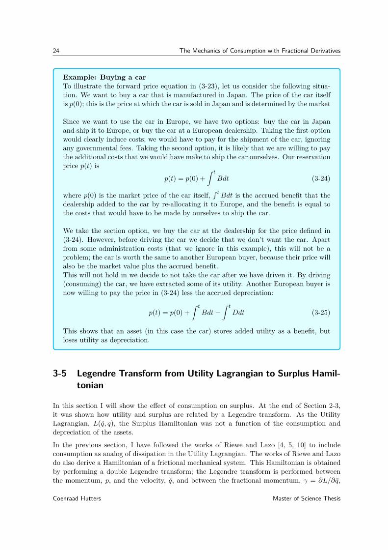
Example: Buying a carTo illustrate the forward price equation in (3-23), let us consider the following situa-tion. We want to buy a car that is manufactured in Japan. The price of the car itselfis p(0); this is the price at which the car is sold in Japan and is determined by the market
Since we want to use the car in Europe, we have two options: buy the car in Japanand ship it to Europe, or buy the car at a European dealership. Taking the first optionwould clearly induce costs; we would have to pay for the shipment of the car, ignoringany governmental fees. Taking the second option, it is likely that we are willing to paythe additional costs that we would have make to ship the car ourselves. Our reservationprice p(t) is
p(t) = p(0) +∫ t
Bdt (3-24)
where p(0) is the market price of the car itself,∫ tBdt is the accrued benefit that the
dealership added to the car by re-allocating it to Europe, and the benefit is equal tothe costs that would have to be made by ourselves to ship the car.
We take the section option, we buy the car at the dealership for the price defined in(3-24). However, before driving the car we decide that we don’t want the car. Apartfrom some administration costs (that we ignore in this example), this will not be aproblem; the car is worth the same to another European buyer, because their price willalso be the market value plus the accrued benefit.This will not hold in we decide to not take the car after we have driven it. By driving(consuming) the car, we have extracted some of its utility. Another European buyer isnow willing to pay the price in (3-24) less the accrued depreciation:
p(t) = p(0) +∫ t
Bdt−∫ t
Ddt (3-25)
This shows that an asset (in this case the car) stores added utility as a benefit, butloses utility as depreciation.
3-5 Legendre Transform from Utility Lagrangian to Surplus Hamil-tonian
In this section I will show the effect of consumption on surplus. At the end of Section 2-3,it was shown how utility and surplus are related by a Legendre transform. As the UtilityLagrangian, L(q, q), the Surplus Hamiltonian was not a function of the consumption anddepreciation of the assets.
In the previous section, I have followed the works of Riewe and Lazo [4, 5, 10] to includeconsumption as analog of dissipation in the Utility Lagrangian. The works of Riewe and Lazodo also derive a Hamiltonian of a frictional mechanical system. This Hamiltonian is obtainedby performing a double Legendre transform; the Legendre transform is performed betweenthe momentum, p, and the velocity, q, and between the fractional momentum, γ = ∂L/∂q,
Coenraad Hutters Master of Science Thesis

3-5 Legendre Transform from Utility Lagrangian to Surplus Hamiltonian 25
and the fractional derivative q.
However, using this Legendre transform to derive a Fractional Surplus Hamiltonian from theFractional Surplus Lagrangian leads to the incorrect result that an increase in depreciation hasa positive effect on the surplus, see Appendix A-2. Therefore, I propose that the FractionalSurplus Hamiltonian should be obtained by performing the Legendre transform only overthe price (generalized momentum), p, and the flow variable (velocity), q. I motivate thisproposition by the observation that whereas the price (generalized momentum) is a conservedproperty, there is no conservation law for the expense (fractional momentum).
The Fractional Surplus Hamiltonian is derived by performing a Legendre transform on theLagrangian over the velocity.
H = ∂L
∂qq − L (3-26)
Substituting the definition of reservation price (p ≡ ∂L/∂q), the surplus can be written as
H = pq − L (3-27)
The total derivative of this Surplus Hamiltonian, which I name the Surplus Statement3, dH,is
dH = ∂H
∂pdp+ ∂H
∂qdq + ∂H
∂qdq (3-28)
This implies that the surplus changes with the change in price, expense, and stock multi-plied by the factors ∂H
∂p ,∂H∂γ , and
∂H∂q , respectively. These three factors can be identified by
evaluating the total derivative of the Fractional Utility Lagrangian
dL = ∂L
∂qdq + ∂L
∂qdq + ∂L
∂qdq (3-29)
Substituting the price, p, yields
dL = pdq + ∂L
∂qdq + ∂L
∂qdq (3-30)
Using the product rule and subsequently moving the term d(pq) to the left-hand side resultsin
d(pq − L) = qdp− ∂L
∂qdq − ∂L
∂qdq (3-31)
Observing that the left-hand side is equal to the Surplus Hamiltonian (3-27) we find thefollowing Hamilton equations
∂H
∂p= q,
∂H
∂q= −∂L
∂q,
∂H
∂q= −∂L
∂q, (3-32)
Substituting the equalities ∂L∂q = γ and ∂L
∂q = B we get that the Surplus Statement, dH, is
dH = qdp− γdq −Bdq (3-33)
That is, the change in surplus is a result of3Using terminology from accounting; e.g. Income Statement, Cash Flow Statement [13]
Master of Science Thesis Coenraad Hutters

26 The Mechanics of Consumption with Fractional Derivatives
1. the change in price multiplied by the flow,
2. the change in consumption multiplied by the expense, and
3. the change in stock multiplied by the cost
The Fractional Surplus Hamiltonian H(p, q, q) can be linked to the earnings before interestand tax (EBIT 4) in accounting [13]. Comparing the Surplus Statement, dH, to a change inEBIT, I link the first effect to the change in revenue, the second effect to the depreciation,and the third effect to the cost of goods sold.By deriving the Hamiltonian as done in (3-27), the depreciation has a negative effect on theSurplus Statement, dH, corresponding to the negative effect of depreciation on the EBIT.Riewe and Lazo argued that deriving the Hamiltonian as done in (A-1) results in a Hamilto-nian as the total energy in the system [4, 5, 10]. Assuming their Hamiltonian is indeed thetotal energy, this implies that surplus is not analogous to energy in general, but to availability;whereas availability is the energy available to perform work, surplus is the cash flow availableto perform economic activity.
3-6 Surplus Hamiltonian in Port-Hamiltonian Control
So far, this chapter concerned the first objective of this thesis: modeling consumption aseconomic analog of dissipation in the Lagrangian and Hamiltonian formalism. The secondobjective of this thesis is to use control methods from port-Hamiltonian systems theory tocontrol an economic system in the presence of consumption. In the previous section, theLegendre transform was used to relate the economic fundamental concept of utility to theHamiltonian description that is used in port-Hamiltonian systems theory.5 Now, the goal isto include the Fractional Surplus Hamiltonian (3-27) in the port-Hamiltonian formalism.However, there is a problem with including the Fractional Surplus Hamiltonian (3-27) in theport-Hamiltonian formalism. Whereas the Hamilton’s equations of a traditional Hamiltoniansystem can be expressed with Poisson brackets (see Paragraph 42 of [12]), this is not the casefor the Fractional Surplus Hamiltonian since the coordinate system (p, q, q) is not canonical.Naively implementing the Surplus Hamiltonian H(p, q, q) in the port-Hamiltonian formalism,we would write q˙q
p
= S
∂H∂q∂H∂q∂H∂p
, (3-34)
where S is some structure matrix. However, such a description cannot be obtained since ˙qis not defined. This implies that the Fractional Surplus Hamiltonian is inadmissible for theport-Hamiltonian formalism.
4EBIT= Revenue - costs and expenses (except interest and tax).5The fractional Lagrangian can be used in the context of optimal control. As mentioned in the introduction,
economists model utility as a Lagrangian in a similar fashion as done in optimal control techniques. TheFractional Utility Lagrangian introduced in this chapter is suitable to be included in optimization. Since thisis not inside the scope of this thesis, I will not discuss this in further detail. Interested readers are referred toSection 5 of [14], where a similar fractional Lagrangian is used in optimal control in the context of a mechanicalsystem with friction.
Coenraad Hutters Master of Science Thesis

3-7 Conclusions 27
For this reason, I leave the port-Hamiltonian control of the Surplus Hamiltonian with frac-tional derivatives as an open problem. In the next chapter, I derive an alternative methodto include consumption as analog of dissipation in the Hamiltonian, using complex-valuedcoordinates. The resulting Complex Hamiltonian is a function of a coordinate pair that iscanonical.
3-7 Conclusions
This chapter addressed the problem that the Utility Lagrangian in economic engineering isnot a function of consumption.
I have shown that with fractional calculus [4, 5, 10], consumption can be included as anindependent variable in the Fractional Utility Lagrangian. Applying the fractional calculusof variations to the principle of maximum utility — stating that economic agents adjusttheir asset stock so as to maximize their utility — results in a fractional Euler-Lagrangeequation that represents the price dynamics. Whereas the classical Euler-Lagrange equationused in economic engineering relates a change in price to an accrued benefit, the fractionalEuler-Lagrange equation relates a change in price to the accrued benefit less the accrueddepreciation from consuming the asset. The classical example of this phenomenon is that thevalue of a car decreases proportional to the distance it has covered over its lifetime.
Performing a Legendre transform on the Fractional Lagrangian results in the Fractional Sur-plus Hamiltonian, which is an extension to the Fractional Surplus Hamiltonian in economicengineering. I showed that the Legendre transform should be performed over the flow ofassets only, rather than over the flow of assets and the consumption, as done in [4, 5, 10].The former results in a Fractional Surplus Hamiltonian that decreases when depreciation in-creases, whereas the latter would result in a Fractional Surplus Hamiltonian that increaseswhen depreciation increases.
In this thesis I aim to apply control formalisms from port-Hamiltonian systems theory toeconomic systems. The Fractional Surplus Hamiltonian is, however, not a function of a setof canonical coordinates. As a result, control formalisms of port-Hamiltonian systems theorycannot be applied to the Fractional Surplus Hamiltonian.
Contributions
1. Consumption is included as an independent variable in the Utility Lagrangian
2. The fractional Euler-Lagrangian equation includes depreciation from consumption inthe price dynamics
3. It was shown that economic surplus is analogous to the availability rather than theenergy in general
Master of Science Thesis Coenraad Hutters

28 The Mechanics of Consumption with Fractional Derivatives
Coenraad Hutters Master of Science Thesis

Bibliography
[1] H. Varian, Intermediate Microeconomics, W.W. Norton & Co., 8th Edition, (2010), pp.54-70
[2] R. Smit, The Interpretation and Application of 300 Years of Optimal Control inEconomics, TU Delft repository, (2018), http://resolver.tudelft.nl/uuid:b119979b-2348-4ca6-8d6b-02c923912d1b
[3] Allison, A., Pearce, C. E. M., Abbott, D., A Variational Approach tothe Analysis of Non-Conservative Mechatronic Systems, (2012), Online available:https://arxiv.org/pdf/1211.4214.pdf
[4] F. Riewe, , Nonconservative Lagrangian and Hamiltonian Mechanics, Physical Review E52,(1996), pp. 1890 - 1899
[5] F.Riewe, Mechanics with fractional derivatives, Physical Review E 55, (1997), pp.3581-3592
[6] A.B. Malinowska, T. Odzijewicz, D.F.M. Torres, Advanced Methods in the FractionalCalculus of Variations, Springer , (2015)
[7] V.V. Tarasova and V.E. Tarasov, Economic Interpretation of Fractional Derivatives,Progr. Fract. Differ. Appl. 3, No. 1, 1-6 (2017)
[8] Oldham, K.B., Spanier, J.,The Fractional Calculus, New York: Dover Publications Inc.,(1974)
[9] M. Klimek, On solutions of linear fractional differential equations of a variational type,Czestochowa: The Publishing Office of Czestochowa University of Technology, (2009)
[10] M.J. Lazo, C. E. Krumreich, The action principle for dissipative systems, Journal ofMathematical Physics 55, (2014)
[11] A.A. Kilbas, H.M. Srivastava ,J.J. Trujillo, Theory and applications of fractional dif-ferential equations, vol 204. North-Holland mathematics studies. Elsevier, Amsterdam,(2006)
Master of Science Thesis Coenraad Hutters
30 Bibliography
[12] L. D. Landau, E.M. Lifshits, Mechanics, Course of Theor. Phys. vol. 1, Pergamon PressLtd., (1969), pp.1-10
[13] S. Bragg, Cost Management Guidebook, 3rd, Accounting Tools, (2017)
[14] Frederico, G.S.F., Lazo, M.J., Fractional Noether’s Theorem With Caputo Derivatives:Constants of Motion for Non-Conservative Systems, Nonlinear Dyn85,(2016), pp. 839-851
Coenraad Hutters Master of Science Thesis

Chapter 4
Complex-Hamiltonian Systems andControl
4-1 Introduction
Although port-Hamiltonian systems theory does account for dissipative systems, it does notinclude the dynamics of dissipation in the Hamiltonian itself, see Section 2-4. Conceptually,this is not in line with the Hamiltonian description of economic engineering where consumption— the economic analog of dissipation — is endogenous to the economic agent, as shown in Sec-tion 2-3. Furthermore, the passivity-based control and control by interconnection formalismsfrom port-Hamiltonian systems are constrained by the dissipative elements, see Section 2-4-3.The latter is known as the dissipation obstacle [1, 2, 3, 4].
Problem
1. In port-Hamiltonian systems theory the dynamics of dissipation are handled sep-arately from the Hamiltonian
2. Control formalisms in port-Hamiltonian systems theory are constrained by thedissipation obstacle
In this chapter, I develop a theory that both models dissipation as an endogenous effect of theHamiltonian and bypasses the dissipation obstacle. To achieve this, I propose the followingsolution.
Solution
Include the dynamics of dissipative elements in the Hamiltonian by using complex statevariables.
Master of Science Thesis Coenraad Hutters

32 Complex-Hamiltonian Systems and Control
This chapter is structured as follows. Section 4-2 introduces the Hamiltonian description of(damped) harmonic oscillators with complex state variables. Section 4-4 joins the Complex-Hamiltonian description and the port-based description of port-Hamiltonian systems, result-ing in complex-port-Hamiltonian systems. Section 4-5 applies the control formalisms fromport-Hamiltonian systems theory to complex-port-Hamiltonian systems. Section 4-6 con-cludes and discusses the chapter.
In order to relate the developments I make in this chapter to port-Hamiltonian theory, Iwill consider mechanical systems only. Chapter 5 applies the developed formalisms to theeconomic agent.
4-2 From Modeling to Complex-Hamiltonian Systems
In this section I show how physical systems can be described as Complex-Hamiltonian systems.This will be done in a constructive manner using the mechanical harmonic and dampedharmonic oscillator as fundamental systems. The purpose of this section is to introducethe similarity between the Complex-Hamiltonian and the port-Hamiltonian description. TheComplex-Hamiltonian and the complex equations of motion are formalized in Section 4-3.
4-2-1 Harmonic Oscillator
Complex Equation of Motion
Figure 4-1: Mass-Spring system as har-monic oscillator Figure 4-2: Geometric representation of (4-
1). The equation of motion can simply beread off using the structure of the complexplane. The dash-dotted circle represents theHamiltonian H = aa.
Consider the mass-spring system in Figure 4-1. It is well-known that the systems time evo-lution can be written either as a set of two coupled first-order equations or one second-orderequation of motion. Less known is the fact that it can be written as a single first-orderequation in a complex state variable a as follows, see e.g. [5]
a = −iωna (4-1)
Coenraad Hutters Master of Science Thesis

4-2 From Modeling to Complex-Hamiltonian Systems 33
Here, ωn denotes the natural frequency of the system and the complex-valued state is definedas
a =√V + i
√T =
√k
2 q + i
√1
2mp (4-2)
with V the potential and T the kinetic energy. The complex equation of motion (4-1) is easilyverified geometrically, see Figure 4-2.
Hamilton’s Equation
Alternatively, the system can be described using Hamilton’s equations. In port-Hamiltoniansystems this is done in matrix form, see [3](
qp
)= J
(∂H∂q∂H∂p
), H = 1
2kq2 + p2
2m (4-3)
where J is a skew-symmetric structure matrix such that J2 = −I.
In complex state variables, Hamilton’s equations reduces to a single equation. First noticethat the Hamiltonian for the undamped oscillator becomes:
H = aa (4-4)
as can be verified by substituting (4-2) into this expression. This allows the complex equationof motion to be written as:
a = −iωn∂H∂a
, H = aa (4-5)
Compare this to the port-Hamiltonian formulation. It can be seen that the complex structureJ-matrix is replaced by the factor −i. However, whereas the J-matrix is an abstract matrixwith J2 = −I, the factor −i directly corresponds to the −90 rotation required to go fromthe gradient of H to the direction of a.
4-2-2 Damped Harmonic Oscillator
Complex Equation of Motion
I now extend this analysis to the damped harmonic oscillator.
Expressing the equation of motion of a mass-spring damper system in complex state variables,the complex equation of motion becomes
a = −(β + iωn)a+ βa (4-6)
where β = b2m is the damping coefficient. Figure 4-4 shows a geometric representation of
the complex equation of motion. This is a single first-order equation that replaces the usualsystem given by the A-matrix formalism. The derivation of the complex equation of motion(4-6) is done step-by-step in Appendix D-1.
Master of Science Thesis Coenraad Hutters

34 Complex-Hamiltonian Systems and Control
Figure 4-3: Mass-Spring-Damper Systemas damped harmonic oscillator
Figure 4-4: Complex equation of motion ofa mass-spring-damper system
Hamilton’s Equation
Non-conservative elements are typically not included in the Hamiltonian, see e.g. [6]. InSection 2-4 it was shown that in port-Hamiltonian systems this issue is solved by introducinga dissipation matrix R and representing dissipative systems as(
qp
)= (J −R)
(∂H∂q∂H∂p
), H = 1
2kq2 + p2
2m (4-7)
However, as was reviewed in Section 2-4-3, the R matrix causes the dissipation obstacle inseveral control techniques of port-Hamiltonian systems theory.I now show that damping can be included in the Hamiltonian with complex numbers so thatthe equation of motion of a damped system can be written as a Hamilton’s equation.I introduce the complex-valued Hamiltonian of a damped system (see Section 4-3):
H(a) = (1− iζ)aa− 12 iζa
2 + 12 iζa
2 (4-8)
where ζ = b2√km
is the damping ratio. Following the same procedure as in (4-5), I find theexpression for the equation of motion as
a = −iωn∂H∂a
, H = (1− iζ)aa− 12 iζa
2 + 12 iζa
2 (4-9)
This expression indeed coincides with the expression found in (4-6). Again, compare thisresult to the port-Hamiltonian formulation in (4-3-5).
By describing a system with complex state variables, the equation of motion can be definedas a single Hamilton’s equation even in the presence of damping. This allows the structure ofthe Hamilton’s equation, −i, to be maintained in the presence of damping. The dissipationmatrix R used in port-Hamiltonian systems (4-3-5) thus becomes obsolete. In Section 4-5 Iwill show that this is an important result for solving the dissipation obstacle.
Coenraad Hutters Master of Science Thesis

4-3 The Complex Hamiltonian 35
4-3 The Complex Hamiltonian
In this section, I show that the Complex-Hamiltonian of a damped harmonic oscillator isdefined on a complex symplectic structure. This will show to be an important result regardingthe dissipation obstacle.First I define the complex state, a. Then I define the complex equation of motion, a, asthe Poisson bracket Finally, I derive the Complex-Hamiltonian, H, of a damped harmonicoscillator.
4-3-1 The Complex State
For a set of symplectic state variables (qj , pj), j = 1, . . . , n, the corresponding complex statesare (see e.g. [5, 7])
aj = α1,jqj + iα2,jpj , (4-10)Here, the α’s are some complex constants.For the mechanical oscillator, I choose these complex coordinate so that iso-energetic curvesare simply represented by circles on the complex plane. This is achieved by choosing a as
aj =√Vj(qj) + i
√Tj(pj) =
√kj2 qj + i
√1
2mjpj , (4-11)
with Vj(qj) and Tj(pj) the potential and kinetic energy, respectively. A circle, aa, on thecomplex plane coincides with the Hamiltonian of a conservative system on the (q, p)−plane
H(q, p) = p2
2m + 12kq
2,
implying that a circle on the complex plane indeed represents constant energy.
4-3-2 The Complex Poisson Bracket
Following the lecture notes of Svistunov [7], I define the time evolution of a system as thecanonical Poisson bracket between the complex state, a, and the Complex-Hamiltonian, H
a ≡ a,H (4-12)
In matrix form, the complex Poisson bracket can be written as
A,B = Ω∂ᵀA
∂a J∂B
∂a , (4-13)
where, the complex state vector, a ∈ C2n, is constructed as n pairs of complex states, aj , andtheir complex conjugate, aj , for j = 1, . . . n. Matrix Ω is constructed as
Ω =
ρ1 0 . . . 0 00 ρ1 . . . 0 0...
... . . . ......
0 0 . . . ρn 00 0 . . . 0 ρn
, (4-14)
Master of Science Thesis Coenraad Hutters

36 Complex-Hamiltonian Systems and Control
with ρj = (α1,jα2,j + α1,jα2,j), for j = 1, . . . n [7]. For the complex state in (4-11) this implies
ρj =√
kjmj
= ωn, is the natural frequency.
Matrix J is constructed as
J =
0 −i . . . 0 0i 0 . . . 0 0...
... . . . ......
0 0 . . . 0 −i0 0 . . . i 0
(4-15)
Notice that we have that J 2 = −I. Compare this to the symplectic matrix of the Hamilton’sequations on the (q, p)−plane
J =(
0 1−1 0
)(4-16)
for which it holds that J2 = −I.
Since the Poisson bracket (4-13) is canonical, it obeys the rules of anticommutivity, bilinearity,Leibniz’s rule and Jacobi’s identity. More importantly, the Poisson bracket satisfies H =H,H = 0. The latter observation means that the Complex Hamiltonian is a constant ofthe motion, i.e. it is a conserved property.
H = H,H = 0 (4-17)
4-3-3 The Complex Hamilton’s Equations
For a simple (damped) harmonic oscillator with complex state a ∈ C2, (4-12) and (4-13)imply that the complex equation of motion is
a = a,H = ωn
(∂a
∂a
∂a
∂a
)(0 −ii 0
)∂H∂a
∂H∂a
= −iωn∂H∂a
(4-18)
By complex conjugation it immediately follows that
˙a = a,H = ωn
(∂a
∂a
∂a
∂a
)( 0 i−i 0
)∂H∂a
∂H∂a
= iωn∂H∂a
(4-19)
I will refer to (4-18) and (4-19) as the Complex Hamilton’s equations. This implies thatthe Complex-Hamiltonian is— as is the classical Hamiltonian— the generator of the time-evolution of the system. Also similar to classical Hamiltonian mechanics, the Complex Hamil-ton’s equations have an equivalent expression in terms of the canonical Poisson bracket. Thelatter implies that the complex coordinate space (a, a) is canonical, see e.g. [8].
Coenraad Hutters Master of Science Thesis

4-3 The Complex Hamiltonian 37
4-3-4 The Complex Hamiltonian of a Damped Harmonic Oscillator
In this section I derive the Complex Hamiltonian of a damped harmonic oscillator. TheComplex Hamiltonian is derived by comparing the complex equation of motion derived fromthe definition of the complex state (4-11) and the Complex Hamilton’s equations.
For a damped harmonic oscillator, the complex equation of motion and its conjugate are (seeAppendix D-1 for the derivation)
a = −(β + iωn)a+ βa (4-20)˙a = βa− (β − iωn)a (4-21)
From the Complex Hamilton’s equations, (4-18) and (4-19), we also have that
a = −iωn∂H∂a
(4-22)
˙a = iωn∂H∂a
(4-23)
Substituting (4-20) and (4-21) in the Complex Hamilton’s equation yields
−(β + iωn)a+ βa = −iωn∂H∂a
(4-24)
βa− (β − iωn)a = iωn∂H∂a
(4-25)
Using β = ζωn, the above equations can be rewritten as
−(iζ + 1)a+ iζa = ∂H∂a
(4-26)
−iζa+ (iζ + 1)a = ∂H∂a
(4-27)
Integrating these equalities with respect to a and a, respectively, we find the Complex Hamil-tonian (up to a constant) as
H = (1− iζ)aa− 12 iζa
2 + 12 iζa
2 (4-28)
Alternatively, the Complex Hamiltonian, H, can be written as
H = E − iD, (4-29)
with E and D the mechanical energy and the dissipation function, respectively. The mechan-ical energy, E , was already evaluated in Section 4-3-1 as
E = aa (4-30)
This leaves the dissipation function, D, as
D = 12ζ(a2 + 2aa− a2) (4-31)
Master of Science Thesis Coenraad Hutters

38 Complex-Hamiltonian Systems and Control
The alternative description of the Complex Hamiltonian can be used to illustrate the geometryof the complex equation of motion, a. The complex equation of motion is generated by theComplex Hamiltonian as the Complex Hamilton’s equation, see (4-18). Using the alternativeexpression for the Complex Hamiltonian (4-29), a can be written as the combination of themotion generated by the energy function, E , and by the dissipation function, D
a = aE − iaD − iωn∂E∂a− ωn
∂D∂a
= −iωn + β(a− a) (4-32)
This construction of the complex equation of motion is visualized in Figure 4-5. Notice thatthe motion generated by the dissipation function, β(a− a), is always directed at the real axisand cancels when Im(a) = 0. This implies that the dissipation is negative proportional tothe momentum.
Figure 4-5: Complex equation of motion, a, generated by the mechanical energy, E , and thedissipation function, D, for different states. The motion generated by the dissipation function isalways directed at the real axis and cancels when Im(a) = 0. This implies that the dissipation isnegative proportional to the momentum.
4-3-5 Concluding Remarks on the Complex Hamiltonian
In contrast to the classical Hamiltonian, the Complex Hamiltonian can describe dampedharmonic oscillators. In fact, the Complex Hamiltonian is a generalization of the classicalHamiltonian on the complex plane. Indeed, setting ζ = 0 the Complex Hamiltonian (4-28)reduces to the classical Hamiltonian. This is easily verified with the alternative formulationH = E+iD with E and D defined in (4-30) and (4-31), respectively. The Complex Hamiltonianis indeed a Hamiltonian, since it is the generator of the time-evolution of the system, obeyingthe algebra of the canonical Complex Poisson bracket.
The statement that the Complex Hamiltonian is the generalization of the classical Hamilto-nian implies that the Complex Hamilton’s equation is the generalization of the Hamilton’sequation. This is an important result regarding the dissipation obstacle in pH systems theory.
In pH systems, dissipation is accounted for by subtracting a damping matrix, R, from thesymplectic matrix, J . (
qp
)= (J −R)
(∂H∂q∂H∂p
), H = 1
2kq2 + p2
2m
Coenraad Hutters Master of Science Thesis

4-4 Complex-Port-Hamiltonian Systems 39
However, if R 6= 0 the damping matrix, R, clearly violates the symplectic structure of theHamiltonian vector field. In comparison, the Complex-Hamiltonian description of the samesystem is
a = −iωn∂H∂a
(4-33)
This description is the same in the absence and the presence of dissipation; the structure ofthe Complex Hamiltonian vector field is not violated by dissipation.
The algebraic link between the classical Hamiltonian and the Complex Hamiltonian is due tothe link between symplectic and complex geometry [9]. I argue that the complex geometry onwhich the Complex Hamiltonian is defined facilitates a structure that allows damped harmonicoscillators to be described by Hamiltonian mechanics. However, finding the correspondingmanifolds and algebraic groups is beyond the scope of this thesis.
4-4 Complex-Port-Hamiltonian Systems
In this section I employ the Complex Hamiltonian in pH systems theory. The combinationof the Complex-Hamiltonian and pH systems theory will be referred to as the complex-port-Hamiltonian (cpH) theory. The structure of the Complex Hamilton’s equations is not affectedby dissipation. In the cpH description, control formalisms from pH systems are not affectedby the dissipation obstacle. Furthermore, since Complex-Hamiltonians can include damping,the Energy Shaping and Damping Injection formalisms reduce to a single formalism.
4-4-1 Stateful and Stateless Elements
The first implication of the Complex Hamiltonian regarding the port-based approach is thatenergy-storing and energy-dissipating do not have to be treated separately. Whereas thetraditional port-Hamiltonian formalism divides system elements into energy-storing, energy-dissipating and energy-routing elements, the cpH formalism divides elements into two classes.These two classes will be referred to as Stateful, for elements that store a state, and Stateless,for elements that do not store any state, borrowing terminology from computer science. Thecomparison between element classes of cpH and pH systems is summarized in Table 4-1.
The difference in element classes illustrates the difference in pH and cpH systems. All elementsthat can be specified by a Complex-Hamiltonian are stateful elements. In contrast to in pHsystems, this includes dampers. As a result, there is no dissipation matrix in the input-state-output description of a cpH system, as will be shown in the next section.
Complex-Port-Hamiltonian Port-Hamiltonian Physical componentsMasses, inductors, ...Energy-Storing Spring, capacitors, ...Stateful
Energy-Dissipating Damper, resistors, ...Stateless Energy-Routing Gears, wires, transformers, ...
Table 4-1: Classes of elements in complex-port-Hamiltonian, port-Hamiltonian, and the relation-ship to the physical components they describe.
Master of Science Thesis Coenraad Hutters

40 Complex-Hamiltonian Systems and Control
4-4-2 Input-State-Output Description
In this section, I introduce physical inputs and outputs to the Complex Hamiltonian de-scription. Although complex state variables are useful for incorporating damping in theHamiltonian description of mechanics, they are inconvenient to use as physical inputs andoutputs, such as forces and velocities. I use the definition of the complex state (4-10) toconvert real-valued physical input and output signals to complex-valued state variables. Thisway, physical inputs and outputs can be used to measure and actuate the system, while thedynamics of the systems are computed with Complex-Hamiltonian mechanics.
The input-state-output description of a cpH system is
a = J∇H+ Guy = Gᵀ∇H
(4-34)
with state vector a ∈ C2n, input vector u ∈ Rm,m ≤ 2n, output vector y ∈ Rm, complexmatrix J : C2n −→ C2n×2n (defined in (4-15)), input matrix G : C2n×m —relating pairs of realstate variables to complex state variables — and the operator ∇H ∈ C2n constructed as1
∇H =(∂H∂a1
∂H∂a1
. . .∂H∂an
∂H∂an
)ᵀ
(4-35)
Comparing the description in (4-34) to the input-state-output description of a pH system(2-14):
x = [J −R]∇H + g(x)uy = gᵀ(x)∇H,
(PH-1)
it can immediately be seen that the descriptions are similar However, whereas in the pHdescription a dissipation matrix, R(x), is needed to account for damping, the cpH descriptionhas no need for the dissipation matrix. See (2-14) for the definitions of the elements in (PH-1).
Note that including physical real-valued inputs and outputs requires the complex conjugatesaj , for j = 1, . . . , n to be incorporated in the input-state-output description. This is a resultof the inverse definitions of the complex state,
q =√
12k (a+ a), p = −i
√m
2 (a− a), (4-36)
Example: Mass-Spring-Damper system with Force input
Consider a linear Mass-Spring-Damper system with mass m, spring constant k, damp-ing constant b, natural frequency ωn =
√km , damping ratio ζ = b
2√km
and Complex-
1∇H is constructed so that J∇H is a shorthand notation for(a1,H a1,H . . . an,H an,H
)ᵀCoenraad Hutters Master of Science Thesis

4-5 Complex-Port-Hamiltonian Control 41
HamiltonianH = (1− iζ)aa− 1
2 iζa2 + 1
2 iζa2 (4-37)
The system is driven by a force acting on the mass, u = F . From the port-basedapproached it follows that the velocity of the system is the output of the system:y = q. From (4-34), the input-state-output description of this system is
(a˙a
)=(
0 −iωniωn 0
)∂H∂a∂H∂a
+
i√
12m
−i√
12m
u
y =(i√
12m −i
√1
2m
)∂H∂a∂H∂a
(4-38)
Notice that the output y can be written as
y =(−i√
12m i
√1
2m
)∂H∂a∂H∂a
=(−i√
12m i
√1
2m
)(−iω−1n
˙aiω−1n a
)=√
12k (a+ ˙a) = q
(4-39)
From the first equation in (4-36) we have that this indeed is the velocity.
4-5 Complex-Port-Hamiltonian Control
In this section, I apply the control formalisms from pH systems theory (see Appendix C)to cpH systems. First I show that the energy flow at the port of the system is the productof the input and the output signals. Then, I apply the passivity based control and controlby interconnection formalisms to the cpH systems description. It will appear that in bothformalisms cpH systems are not affected by the dissipation obstacle.
4-5-1 Passivity-Based Control
A key concept in pH systems theory is passivity [3]. A system is said to be passive if it is notable to autonomously generate energy along its trajectories. An important equation in thistechnique is the energy-balance equation [4]
H[x(t)]−H[x(0)]︸ ︷︷ ︸stored energy
=∫ t
0uᵀ(s)y(s)ds︸ ︷︷ ︸
supplied energy
− d(t)︸︷︷︸dissipated energy
Master of Science Thesis Coenraad Hutters

42 Complex-Hamiltonian Systems and Control
In the passivity based control (PBC) formalism , it is assumed that a perfect model of a plantis provided and no noise is acting on the system or the measurement, i.e. static control. ThePBC formalism exploits the physical structure and the energy balance of physical systems[10, 11, 12]. For an actuated system, the energy balance states that the stored energy isequal to the supplied energy minus the dissipated energy. With controls, a desired amount ofstored energy can be realized by supplying additional energy and increasing the dissipationto render a system closed-loop passive [3].
The first occurrence of the dissipation obstacle in pH systems arises from pervasive dissipation[4]. The power balance of a passive system with input-output description (PH-1) is
dH
dt= ∇Hᵀx
= ∇Hᵀ ([J −R]∇H + g(x)u)= −∇HᵀR∇H︸ ︷︷ ︸
d(x)
+uᵀy(PH-2)
Assume that the control objective is to steer the system to a desired equilibrium x∗ ∈ Rn.Since the energy flow, dH/dt, should be zero at x∗, we have that for a dissipative system,R > 0, the dissipated power has to be compensated by the controller:
u∗ᵀy∗ = ∇ᵀH(x∗)R(x∗)∇H(x∗) (PH-3)
where u∗ and y∗ are the input and output at the equilibrium, respectively. However, thepower that can be extracted from a passive system is bounded [16]. This implies that if thesystem dissipates power at the equilibrium —a phenomenon known as pervasive dissipation—it cannot be stabilized by a passive controller. Therefore, only systems for which it holds that
R(x∗)∇H(x∗) = 0 (PH-4)
can be stabilized with passive controllers. Systems for which (C-25) does not hold are con-strained by the dissipation obstacle [4]
Now compare this to the same situation for a cpH description. From the cpH input-state-output description in (4-34) it can be derived that the energy flow at the port of a cpH systemis
dHdt
= ∇Hᵀa
= ∇HᵀJ∇H+∇HᵀGu= yᵀu
(4-40)
Since the Complex Hamilton’s equation is embedded in y, (4-40) returns the equation ofmotion with the dissipation accounted for. If we steer the cpH system to a desired equilibriuma∗ ∈ Cn, the complex Hamiltonian flow, dH/dt should be zero at a∗. This results in
y∗ᵀu∗ = 0 (4-41)
Coenraad Hutters Master of Science Thesis

4-5 Complex-Port-Hamiltonian Control 43
Compare (4-41) to (PH-3). In (PH-3), the system can only be stabilized with a passivecontroller if condition (PH-4) holds. In (4-41) this is clearly not the case. The dissipationobstacle is thus bypassed in the cpH description.
Rather than describing the energy flow at the port of the storage element, as done in pHsystems, the energy flow of a cpH system is described at the port of the stateful element. Fora damped harmonic oscillator, the stateful element represents the entire physical system.
From the energy flow at the port of a cpH system (4-40), we can obtain a control law, u, thatrenders the closed-loop system passive. The most straightforward choice for this control lawis u = −Ky where K is a positive constant. Indeed, this control law results in the followingenergy flow at the port of the system
dHdt
= −yᵀKy ≤ 0 (4-42)
Since the energy of this system is always decreasing, the stability of the system is guaranteed.
4-5-2 Energy-Shaping and Damping Injection
To emphasize the advantage of using the cpH systems description for the design of controllerswith respect to using the pH description, I first summarize the energy-shaping and damping-injection (ES-DI) formalism for a pH system and then show the simplicity of the same methodfor a cpH system. Moreover, I show how the dissipation obstacle that affects the (ES-DI)formalism for a pH system is bypassed in the cpH description.
ES-DI in PH Systems
Stabilization via energy balancing [4] is a control method that uses the additive propertyof the Hamiltonian. A controller with added energy function Ha can be designed so that adesired closed-loop energy function Hd is obtained
Hd(x) = H(x) +Ha(x) (PH-5)
If Hd has a minimum at the desired equilibrium x∗, the system will be stable.
In [7] this technique is further developed by introducing a damping injection input in orderto ensure convergence of the state trajectories to the desired equilibrium. This procedureis known as Energy-shaping and damping injection (ES-DI). Note that since the classicalHamiltonian does not represent damping, damping injection has to be implemented separatelyfrom energy-shaping.
For a pH plant such as in (2-14) the ES-DI method attempts to obtain a desired closed-loopsystem
x = (J(x)−Rd(x))∇Hd(x) (PH-6)
where Rd is the desired damping matrix
Rd(x) = R(x) + g(x)Kd(x)gᵀ(x)
with damping injection matrix Kd. The desired Hamiltonian Hd is defined in (C-5).
Master of Science Thesis Coenraad Hutters

44 Complex-Hamiltonian Systems and Control
The desired closed-loop dynamics can be realized with control input
u(x) = uES(x) + uDI
where the energy shaping input is generated by the added energy Hamiltonian Ha and thedamping injecting input generated by desired Hamiltonian Hd
uES = (gᵀ(x)g(x))−1gᵀ(x)[J(x)−R(x)]∂Ha
∂x(x)
uDI = −Kd(x)gᵀ(x)∂Hd
∂x(x)
The added energy function Ha(x) can then be found solving the following set, see equation(15.18) of [3] [
g⊥(x)[J(x)−R(x)]gᵀ(x)
]∂Ha
∂x(x) = 0 (PH-7)
The solution for Ha that satisfies x∗ = argmin(Hd = H +Ha) is then selected.
However, the PDE’s in (PH-7) imply that the controlled state cannot be affected by damping.Since in physical systems states are in general affected by damping, this implication reducesthe applicability of the ES-DI method. This is known as the dissipation obstacle shown ine.g. Section 15.7 of [3].
ES-DI in CPH Systems
The Complex-Hamiltonian acts as both the generator of the equations of motion of the systemand as an energy function. In (C-5) it was shown how a synthesized additive energy functionHa(x) can be added to the energy function of the plant in order to obtain a desired energyfunction Hd. For cpH systems, this results in a Hamiltonian balance equation:
Hd(a) = Hp(a) +Hc(a) (4-43)
Since the controller Hamiltonian2 Hc(a) uses the same state as the plant Hp(a), the closed-loop dynamics are obtained as the Poisson bracket (4-13) between the state and the desiredHamiltonian Hd. From the sum rule in differentiation we have that the desired closed-loopequation of motion is
ad = a,Hd = a,Hp+ a,Hc (4-44)
Compare this to (PH-6) in a pH system. Since the Complex Hamiltonian can include damping,the damping injection is done simultaneously with the energy-shaping in the Hamiltonianbalance equation (4 − 43). As I will now show, the ES-DI formalism,— from (C-5) up to(PH-7)— is reduced to (4-43) and (4-44).
2I use the term controller Hamiltonian Hc rather than added energy Ha, since in contrast to the addedenergy Hamiltonian in pH systems, the complex controller Hamiltonian, Hc, can also inject damping.
Coenraad Hutters Master of Science Thesis

4-5 Complex-Port-Hamiltonian Control 45
For a CpH system with input-state-output description
a = J∇H(a) + Gu,y = Gᵀ∇H(a),
(4-45)
Energy-Shaping and Damping Injection (ES-DI) —see Section C-0-2— can be used to obtainthe desired closed-loop system
ad = J∇Hd(a) (4-46)The desired Hamiltonian Hd is found using (4-43) so that it has a minimum at some desiredequilibrium a∗:
a∗ = arg min(Hd(a)) (4-47)The desired closed-loop dynamics (4-46) can be achieved by introducing the feedback law
u = (GᵀG)−1GᵀJ∇Hc(a) = a,Hc (4-48)
as control input u of the system in (4-45). This indeed corresponds to the closed-loop equationof motion described by the Poisson bracket (4-44):
ad = J∇H(a) + J∇Hc(a) = a,H+ a,Hc (4-49)Substituting (4-46) and (4-48), this can be rewritten as
u = ad − a = a,Hd − a,H (4-50)
The simplicity of the above expression for the control law, u, is due to ability of Complex-Hamiltonians to include damping. Whereas the Hamiltonian dynamics of a controller inpH systems can only generate the energy shaping input, the dynamics of a CpH controllergenerates both the energy shaping and dissipation injection inputs. For a CpH system, theEnergy-Shaping and Damping-Injection formalisms are thus combined in a single formalism.More importantly, the controller Hamiltonian is a solution to the set(
G⊥(a)J (a)Gᵀ
)∇Hc(a) = 0 (4-51)
where G⊥(a) is the left-annihilator of G(a).In the previous Section in was shown that the PDE’s in (PH-7) imply that the controlledstate cannot be affected by damping: the dissipation obstacle. The set of PDE’s in (4-51)clearly does not imply that the to be shaped state cannot be affected by damping. Therefore,the dissipation obstacle is bypassed in the cpH description.Bypassing the dissipation obstacle is the result of the structure of the Complex Hamilton’sequation (or the Complex Hamiltonian vector field). Since the structure is not violated bydamping, the set of PDE’s in (4-51) does not require the to be shaped state to be unaffectedby damping.It should be kept in mind that the cpH theory introduced in the present chapter has so far onlybeen developed for linear damped harmonic oscillators. Therefore, it can not be concludedthat using Complex-Hamiltonians will solve the dissipation obstacle in port-Hamiltonian sys-tems in general. This needs to be further researched.
Master of Science Thesis Coenraad Hutters

46 Complex-Hamiltonian Systems and Control
Example: Energy-Shaping and Damping InjectionConsider a linear Mass-Spring-Damper system with mass m, spring constant k, damp-ing constant b, natural frequency ωn =
√km , damping ratio ζ = b
2√km
, input matrix
G =(i√
12m −i
√1
2m
)ᵀ. The Complex-Hamiltonian of the system is
H = 12(a a
)( −iζ (1− iζ)(1− iζ) iζ
)(aa
)= 1
2aᵀHa (4-52)
The input-state-output description of this system is
(a˙a
)=(
0 −iωniωn 0
)∂H∂a∂H∂a
+
i√
12m
−i√
12m
u
y =(i√
12m −i
√1
2m
)∂H∂a∂H∂a
(4-53)
Suppose we want to stabilize the system around a desired equilibrium (q, p) = (q∗, 0)or, in complex state variables, a∗ = a∗ =
√k2q∗.
The desired Hamiltonian, Hd, thus is
Hd = 12(a− a∗
)ᵀ( −iζ (1− iζ)(1− iζ) iζ
)(a− a∗
)(4-54)
Figure 4-6: Trajectory of autonomoussystem. The dashed circles representiso-energetic lines. a∗ is the desiredforced equilibrium
Figure 4-7: Signal trajectory of positionq for the autonomous system.
From (4-50) we can immediately find the control law that results in the desired closed-loop dynamics as
u = a,Hd − a,H (4-55)
Coenraad Hutters Master of Science Thesis

4-5 Complex-Port-Hamiltonian Control 47
The controller that achieves the desired closed-loop dynamics is specified by the Hamil-tonian
Hc = iζ (a(a∗ − a∗) + a(a∗ − a∗))− aa∗ − aa∗ − a∗a∗ (4-56)
Verifying that Hc is indeed a solution for (4-51)(G⊥(a)J (a)Gᵀ
)∇Hc(a) =
(iωn −iωni√
12m −i
√1
2m
)(−iζ(a∗ − a∗)− a∗iζ(a∗ − a∗)− a∗
)= 0, (4-57)
with left-annihilator G⊥ =(1 1
)and using that a∗ = a∗.
Figure 4-8: Trajectory of system stabi-lized around forced equilibrium a∗
Figure 4-9: Position signal of systemstabilized around forced equilibrium.
Now suppose we want to achieve the closed-loop dynamics
ad = −(δ + iψ)(a− a∗) + δ(a− a∗) (4-58)
Here, δ is the closed-loop damping coefficient and ψ is the closed-loop frequency.This implies that the controller law is
u = a,Hc = (δ − β︸ ︷︷ ︸DI
)(a− a)− i(ψ − ωn︸ ︷︷ ︸ES
)a+ (δ + iψ)a∗ − δa∗︸ ︷︷ ︸Forced equilibrium
(4-59)
From (4-43), the controller Hamiltonian is simply found as
Hc = 12(a− a∗
)ᵀ( −iDd Ed − iDd
Ed − iDd iDd
)(a− a∗
)−H (4-60)
with Dd = δ/ωn and Ed = ψ/ωn.
Master of Science Thesis Coenraad Hutters
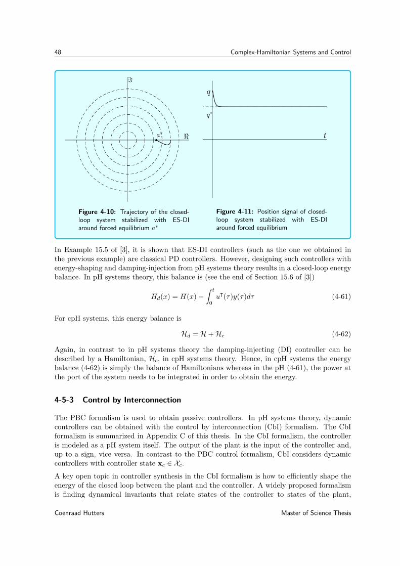
48 Complex-Hamiltonian Systems and Control
Figure 4-10: Trajectory of the closed-loop system stabilized with ES-DIaround forced equilibrium a∗
Figure 4-11: Position signal of closed-loop system stabilized with ES-DIaround forced equilibrium
In Example 15.5 of [3], it is shown that ES-DI controllers (such as the one we obtained inthe previous example) are classical PD controllers. However, designing such controllers withenergy-shaping and damping-injection from pH systems theory results in a closed-loop energybalance. In pH systems theory, this balance is (see the end of Section 15.6 of [3])
Hd(x) = H(x)−∫ t
0uᵀ(τ)y(τ)dτ (4-61)
For cpH systems, this energy balance is
Hd = H+Hc (4-62)
Again, in contrast to in pH systems theory the damping-injecting (DI) controller can bedescribed by a Hamiltonian, Hc, in cpH systems theory. Hence, in cpH systems the energybalance (4-62) is simply the balance of Hamiltonians whereas in the pH (4-61), the power atthe port of the system needs to be integrated in order to obtain the energy.
4-5-3 Control by Interconnection
The PBC formalism is used to obtain passive controllers. In pH systems theory, dynamiccontrollers can be obtained with the control by interconnection (CbI) formalism. The CbIformalism is summarized in Appendix C of this thesis. In the CbI formalism, the controlleris modeled as a pH system itself. The output of the plant is the input of the controller and,up to a sign, vice versa. In contrast to the PBC control formalism, CbI considers dynamiccontrollers with controller state xc ∈ Xc.
A key open topic in controller synthesis in the CbI formalism is how to efficiently shape theenergy of the closed loop between the plant and the controller. A widely proposed formalismis finding dynamical invariants that relate states of the controller to states of the plant,
Coenraad Hutters Master of Science Thesis

4-5 Complex-Port-Hamiltonian Control 49
decreasing the degrees of freedom in the choice of possible controllers. This formalism, knownas the Energy-Casimir formalism, can however not be applied to states that are subject todamping; as the PBC formalism, the CbI formalism is affected by the dissipation obstacle.For a summary of the CbI formalism, the Energy-Casimir formalism, the dissipation obstacle,as well as for references to the literature, the reader is referred to Appendix C-0-3.
In this Section, I integrate the CbI formalism in cpH systems theory. The starting point of theCbI formalism is that a controller is modeled as a cpH system itself. That is, the controllerhas a Hamiltonian Hc(ac), with controller state ac, and a port connecting the controller toits environment. The input-state-output description of the controller is
ac = Jc∇Hc + Gcucyc = Gᵀc∇Hc
(4-63)
with natural frequency of the controller ωc, controller-state vector ac ∈ C2v, input vectoruc ∈ Rw, w ≤ 2v, output vector yc ∈ Rw, complex structure matrix3 Jc : C2v −→ C2v×2v,input matrix Gc : C2v×w, and the operator ∇Hc ∈ C2v constructed as
∇Hc =(∂Hc∂ac,1
∂Hc∂ac,1
. . .∂Hc∂ac,n
∂Hc∂ac,n
)ᵀ
(4-64)
A closed-loop system can be achieved by interconnecting a plant with input-output description(4-34) and a controller (4-63). Using a negative feedback interconnection implies
uc = y, u = −yc (4-65)
This results in a closed-loop system with input-state-output description
(aac
)=(Jp −GpGᵀcGcGᵀp Jc
)(∇Hp∇Hc
)(yyc
)=(Gᵀp 00 Gᵀc
)(∇Hp∇Hc
) (4-66)
with state vector a ∈ C2n, input vector u ∈ Rm,m ≤ 2n, output vector y ∈ Rm, complexmatrix J : C2n −→ C2n×2n (defined in (4-15)), input matrix G : C2n×m, and the operator∇Hp ∈ C2n as defined in (4-35).
Comparing the closed-loop system in (4-66) to a closed-loop system obtained with CbI in pHsystems theory (see (C-0-3)), we notice that the cpH description does not contain a dissipationmatrix. This is again an important result.
In the Energy-Casimir formalism for pH systems, a Casimir function is found as a solutionF (x) for (
−∂ᵀF (x)x
Inc
)(J(x)−R(x) −g(x)gᵀc (ξ)gc(ξ)gᵀ(x) Jc(ξ)−Rc(ξ)
)= 0 (PH-8)
3The structure matrix is constructed as (4-15). Here, the natural frequency is that of the controller.
Master of Science Thesis Coenraad Hutters

50 Complex-Hamiltonian Systems and Control
However, the equality R(x)∂F/∂x = 0 implies that the to be shaped states cannot be affectedby damping [16]. This is known as the dissipation obstacle for the CbI formalism.As for pH systems, Casimir functions for cpH systems (4-66) can be found by relating thestates of the plant to the states of the controller. This can be done by finding dynamicalinvariants (Casimirs) for the closed-loop system [3, 13, 14, 15, 16]. In general, this impliesfinding functions C(a,ac) that satisfy4
(∂ᵀC∂a
∂ᵀC∂ac
)×(Jp −GpGᵀcGcGᵀp Jc
)= 0 (4-67)
and present a Lyapunov candidate function
V = Hp +Hc + C (4-68)
that has a minimum at (a∗,a∗c).The typical candidate function used in pH systems, expressed in complex state variablesbecomes
C(a, ac) = ac −F(a) = κ (4-69)where F(a) is some differentiable function and κ is some constant. With the Casimir candi-date, C(a, ac), the closed-loop energy can be written as
Hcl = H(a) +Hc(C(F(a) + κ)) (4-70)
The closed-loop energy function is conserved (invariant) if [13, 14, 15]
d
dtC(a, ac) = 0 (4-71)
If this is the case, C is indeed a Casimir function and is independent of the Hamiltonian.A Casimir function is found as a solution F(x) for the following PDE’s(
−∂ᵀF(a)∂ᵀa I
)( Jp −GpGᵀcGcGᵀp Jc
)= 0 (4-72)
Compare (4-72) to (PH-8). Clearly, (4-72) —nor (4-67))— does not imply that dampingcannot act on the complex states that need to be shaped. This implies that the dissipationobstacle in the Energy-Casimir formalism is bypassed by the cpH description
4-6 Conclusions
A Complex-Hamiltonian theory can be developed by defining the equations of motion of adamped harmonic oscillator as the complex Poisson bracket between the state and the Com-plex Hamiltonian. Using this definition, the Complex Hamiltonian can be derived by substi-tuting the known equations of motion of a damped harmonic oscillator. Including the Com-plex Hamiltonian in the port-Hamiltonian formalism generalizes energy-storing and energy-dissipating elements as stateful elements. Contrary to port-Hamiltonian systems, Complex-Port-Hamiltonian systems include the effect of dissipation in the Hamilton’s equation. This
4Notice that this set of PDE’s is the complex equivalent of the set of PDE’s in the lossless case of pHsystems. See equation (15.9) of Van Der Schaft [3]
Coenraad Hutters Master of Science Thesis

4-6 Conclusions 51
has two main results. The first result is that the Energy-Shaping and Damping-Injectioncontrol formalism reduces to a single Complex-Hamiltonian balance function. The second,and most important, result is that the control formalisms for a Complex-Port-Hamiltoniansystems is not affected by the dissipation obstacle.
I conclude that defining the complex equation of motion as the Poisson bracket betweenthe state and the Hamiltonian has a crucial step in the derivation of the Complex Hamil-tonian. Resulting from this step, the Complex Hamiltonian always fulfills the requirementsthat it should generate the time-evolution of the system and is a constant of the motion.Furthermore, I argue that this is the reason why the Complex-Hamiltonian is not affectedby the dissipation obstacle. The control formalisms from port-Hamiltonian systems theoryare defined for systems with a Poisson algebra. The dissipation matrix in port-Hamiltoniansystems, however, violates the Poisson bracket of the classical Hamiltonian. As a result, thecontrol methods from port-Hamiltonian systems theory fail for dissipative systems. Since theComplex Hamiltonian is defined so that the Poisson bracket defines the equation of motion ofa damped harmonic oscillator, the Complex Hamiltonian bypasses the dissipation obstacle.Proof of these notions is, however, left for further research.
Future work is also needed to relate the Complex Hamiltonian to a Lagrangian, e.g. thefractional Lagrangian in Chapter 3. This would imply that dissipative systems follow afundamental principle. Furthermore, the theory developed in this chapter has only consid-ered linear second-order damped harmonic oscillators. Conceptually, it is possible to modelhigher order systems as interconnected second-order systems, but a structured formalism tomatch the natural frequencies of the individual subsystems has to be developed. Finally, theComplex-Hamiltonian theory may contribute in modeling and controlling dissipative nonlin-ear systems from an energy perspective.
Contributions
1. Damped harmonic oscillators are included in the Hamiltonian formalism
2. The equation of motion of a damped harmonic oscillator is expressed as a canonicalHamilton’s equation
3. Dissipative cpH systems do not violate the symplectic structure, in contrast to dissipa-tive pH systems
4. For cpH systems, the ES-DI method reduces to a single complex equation of motion
5. The dissipation obstacle that affects the control of pH systems is bypassed in cpHsystems
Master of Science Thesis Coenraad Hutters

52 Complex-Hamiltonian Systems and Control
Coenraad Hutters Master of Science Thesis

Bibliography
[1] J. Koopman and D. Jeltsema, Casimir-based control beyond the dissipation obstacle,ArXiv e-prints, (2012).
[2] M. Zhang, R. Ortega, D. Jeltsema, and H. Su, Further Deleterious Effects of the Dissipa-tion Obstacle in Control-by-Interconnection of Port-Hamiltonian Systems, Automatica,vol. 61, (2015), pp. 227-231
[3] A. Van der Schaft, D. Jeltsema, Port-Hamiltonian Systems Theory: An IntroductoryOverview, Foundations and Trends in Systems and Control, vol. 1, no. 2-3, (2014) .pp.173-378
[4] R. Ortega, A. J. Van der Schaft, I. Mareels, and B. Maschke, Putting energy back incontrol, Control Systems, IEEE, vol. 21, no. 2,(2001), pp. 18-33.
[5] H.C. Corben, P. Stehle, Classical Mechanics, 2nd Ed., Wiley & Sons Inc., (1950) , pp193-195
[6] Allison, A., Pearce, C. E. M., Abbott, D., A Variational Approach tothe Analysis of Non-Conservative Mechatronic Systems, (2012), Online available:https://arxiv.org/pdf/1211.4214.pdf
[7] Svistunov, B, Complex Variables in Classical Hamiltonian Mechan-ics, Lecture Notes, University of Massachusetts, (2018), online availabe:https://people.umass.edu/bvs/605ham.pdf
[8] L. D. Landau, E.M. Lifshits, Mechanics, Course of Theor. Phys. vol. 1, Pergamon PressLtd., (1969), pp.135-138
[9] A. Cannas da Silva, Lectures on Symplectic Geometry, Springer, (2001), pp. 67-72
[10] R. Ortega, A. van der Schaft, B. Maschke, and G. Escobar, Interconnection and DampingAssignment Passivity-Based Control of Port-Controlled Hamiltonian Systems, Automat-ica, vol. 38, no. 4, (2002), pp. 585-596
Master of Science Thesis Coenraad Hutters

54 Bibliography
[11] R. Ortega, A. van der Schaft, F. Castanos, and A. Astolfi, Control by Interconnectionand Standard Passivity-Based Control of port-Hamiltonian Systems, Automatic Control,IEEE Transactions on, vol. 53, no. 11, (2008), pp. 2527-2542
[12] R. Ortega and E. GarcÃŋa-Canseco, Interconnection and Damping Assignment PassivityBased Control: A Survey, European Journal of Control, vol. 10, no. 5, (2004), pp. 432-450,
[13] J. Marsden and T. Ratiu, Introduction to Mechanics and Symmetry, New York: Springer,(1994), pp. 35-42
[14] Dalsmo and A. Van der Schaft, On Representations and Integrability of MathematicalStructures in Energy-Conserving Physical Systems, SIAM J. Opt. Control, vol. 37, no.1, (1999) ,pp. 354-369
[15] V. Duindam, A. Macchelli, S. Stramigioli, and H. Bruyninckx, Modeling and Control ofComplex Physical Systems, Springer, (2009).
[16] A. Van der Schaft, L2-gain and Passivity Techniques in Nonlinear Control., SpringerScience & Business Media, (2012).
Coenraad Hutters Master of Science Thesis
Chapter 5
The Mechanics of Consumption withComplex-Hamiltonian Systems
5-1 Introduction
In economic engineering, available surplus is the economic analog of the Hamiltonian frommechanics, see Section 2-3. Modeling an economic agent as a Surplus Hamiltonian systemresults in a description of a trader that is analogous to a mechanical harmonic oscillator.However, the mechanical Hamiltonian only describes conservative systems, see e.g. the intro-duction of [1] and references therein. For the description of an economic agent, this impliesthat consumption (and profits) are not included in the Surplus Hamiltonian.
ProblemThe Surplus Hamiltonian from Economic Engineering is not a function of consumption
In this Chapter, I use the Complex Hamiltonian, developed in Chapter 4, to include con-sumption (and profit) in the Surplus Hamiltonian.
SolutionInclude Consumption in the Surplus Hamiltonian following the Complex Hamiltoniantheory
In Chapter 4, the Complex Hamiltonian was introduced to include dissipative systems in theHamiltonian formalism. In the present chapter, the Complex Hamiltonian will be used toinclude consumption in the Hamiltonian formulation of economic agents [2]. The economictheory of the saving-investment cycle [3, 4] is interpreted in the framework of economic engi-neering in Section 5-2. The Complex Hamiltonian represents the saving function, constructedas the sum of the disposable income function and the consumption function. In Section 5-3, the saving function[4] as Complex Hamiltonian system is reformulated as a cpH system
Master of Science Thesis Coenraad Hutters

56 The Mechanics of Consumption with Complex-Hamiltonian Systems
with physical inputs and outputs. In Section 5-4, control methods of cpH systems theory areapplied to the cpH formulation of the saving function.
5-2 The Saving-Investment Cycle
In the financial system, surplus from one economic agent, e.g. a household, is used to financethe investment of another agent, e.g. a firm. This is known as the saving-investment cycle[3]. The saving, S, of an agent equals their disposable income, Yd, minus their consumption,C, see e.g. [4]
S = Yd − C (ECON-1)
Here, disposable income, Yd, is the income after taxes, social security fees and necessities[5]. The agent is thus free to choose whether to save or consume its disposable income. Theconsumption function, C, does not include the consumption necessary for survival, i.e. foodand shelter; only the consumption of disposable income, C = C(Yd).
5-2-1 Some Preliminaries on the Hamiltonian Surplus Function
The goal of this chapter is to present a prove of concept for the use of the Complex Hamiltonianto model the saving function (ECON-1). As is done in economic engineering theory in general,economic agent is modeled as a simple (damped) mechanical oscillator [?]. The agent isdefined by a single capital asset stock, q, with price p. The disposable income, Yd, is thecapital income obtained by trading the capital asset, q, see Figure 5-1. Here, it is assumedthat the agent has a fixed Trade Frequency, ωT .
Notice that the model only regards disposable income. Zero disposable income does not meanthat the agent is broke; the agent still finances its necessities with its non-disposable income.The capital itself cannot be consumed; the agent can only consume the monetary value ofthe capital after liquidating the capital stock. Depreciation of capital is not considered in themodel.
5-2-2 The Complex Hamiltonian as the Complex Surplus Function
Whereas the Surplus Hamiltonian from economic engineering can only model the surplus fromdisposable income (see Section 2-3), the Complex Hamiltonian can conceptually also includethe surplus from consumption as economic analog of dissipation, see Section 4-3. Modelingthe agent as a Complex-Hamiltonian results in a Complex Surplus Hamiltonian, Σ, as thegenerator of a saving equation corresponding to (ECON-1).
The state of the economic agent is defined by the stock of capital assets, q, and the corre-sponding price, p. Integrating this state in the Complex-Hamiltonian theory, the complexstate is defined as
z ≡ α1q + iα2p (5-1)
Here, α1 and α2 depend on the illiquidity, κ, and the slope of the demand curve (price rigidity),µ, respectively, see section 2-3. Assuming that both the illiquidity and the price rigidity are
Coenraad Hutters Master of Science Thesis

5-2 The Saving-Investment Cycle 57
Figure 5-1: Periodic fluctuation in capital stock due to trade.
linear, the complex economic state is
z =√κ
2 q + i
√1
2µp, (5-2)
Analogous to the Complex Hamiltonian (see Section (4-3)), the Complex Surplus Hamiltonian,Σ, is composed by a real part representing the Disposable Income function, Yd, and animaginary part representing the Consumption function, C.
Σ = Yd − iC (5-3)
The Disposable Income function, Yd, is analogous to the mechanical energy (E in (4-29))1 andthe Consumption function is analogous to the Dissipation function (D in (4-29)). Followingthis analogy, the Disposable Income function of an economic agent with state (5-2) is
Yd = zz (5-4)
When the Consumption, C, is zero and no profits are made by trading the capital, the sur-plus, Σ, is constant. In that case, the Complex Surplus Hamiltonian reduces to the SurplusHamiltonian introduced by economic engineering in Section 2-3.
5-2-3 Damping Ratio as the Marginal Propensity to Consume
Now we will evaluate the analogy between dissipation and consumption. In economics, theconsumption function, C, introduced by Keynes [6], relates consumption to Disposable In-come, Yd [7]. In its simplest form, the Consumption function is a linear function of thedisposable income, see e.g. Chapter 4 of [4]
C = a+ λYd (ECON-2)1For your convenience (4-29): H = E − iD
Master of Science Thesis Coenraad Hutters

58 The Mechanics of Consumption with Complex-Hamiltonian Systems
Here, a is the (constant) autonomous consumption and λ is the marginal propensity to con-sume. The autonomous consumption is the consumption that is independent of the income.Since it is a constant, the autonomous income will not have an influence on the dynamics ofthe economic agent and can therefore be omitted.
In economics, the marginal propensity to consume (MPC) is the change in consumption dueto a change in disposable income [4]
λ = ∆C∆Y (ECON-3)
Substituting the complex Disposable Income function, Yd in (5-4), it follows that the com-plex Consumption function, C, should be proportional to the Disposable Income functionmultiplied by the MPC, λ:
C ∝ λYd
The economic agent generates disposable income by trading capital. However, capital itselfcannot be consumed; the agent first needs to liquidate the capital in order to consume. Thisis the same effect as was found for the damped harmonic oscillator in Chapter 4. The dampedharmonic oscillator can only dissipate kinetic energy. To capture this effect, I will use thedissipative function, D, of the Complex Hamiltonian of a damped harmonic oscillator (4-29)to model the Consumption function:
C := λ
(zz + z2 − z2
2
)(5-5)
This implies that the marginal propensity to consume, λ, is analogous to the mechanicaldamping ratio, ζ. In economics, the MPC is the ratio of the differences in consumption anddisposable income over a given period [4]
MPC ≡ ∆C∆Y (ECON-4)
Substituting the (5-4) and (5-5) this becomes
MPC =∆λ
(zz + z2−z2
2
)∆zz = λ
(∆zz∆zz + ∆(z2 − z2)
2∆zz
)(5-6)
The first fraction on the right-hand side clearly reduces to identity. The second fraction takesvalues between −i and i and vanishes when the interval over which the difference is measuredis set to the economic period2 of the agent. Therefore, it follows that
MPC := λ (5-7)
Comparing the Consumption function, C, in (5-5) with the Complex Hamiltonian of a dampedharmonic oscillator in (4-8), it can be seen that the MPC in the Consumption function isanalogous to the damping ratio, ζ in the Complex Hamiltonian of a mechanical system, seeSection 4-3.
2See Figure 5-1
Coenraad Hutters Master of Science Thesis

5-2 The Saving-Investment Cycle 59
Mathematically, we can also evaluate the instantaneous change in consumption with respectto the disposable income:
Λ = dC
dY= λ
(1 + zdz − zdz
zdz + zdz
)(5-8)
Here, Λ is the instantaneous marginal propensity to consume (iMPC). In contrast to theMPC, the iMPC is not a constant but a complex function. The real part of the iMPC isequal to the MPC (λ) and the imaginary part, generated by zdz−zdz
zdz+zdz , takes values between−iλ and iλ.Modeling an economic agent as a Complex Hamiltonian Surplus function thus implies thatthe damping ratio, ζ, in mechanical systems is analogous to the MPC in economics. Fur-thermore, the model implies that the instantaneous MPC is not constant, but a complexfunction with constant real part (the MPC) and an imaginary oscillation. This fluctuation inthe instantaneous MPC, Λ, is due to the fact that the economic agents first has to liquidateits capital before he can consume its value. This is a similar effect as observed in the Com-plex Hamiltonian of a mechanical system, where the dissipation function in the Hamiltonianaccounts for the fact that damping can only act on the kinetic energy.
5-2-4 Complex Hamilton’s Equation as Saving Equation
Now we evaluate the time-evolution of the complex state, z, following the Complex Hamilton’sequations, see Section 4-3-3. From the theory on Complex Hamiltonians developed in Chapter4, we have that the equations of motion are defined as the Poisson bracket between the stateand the Complex Hamiltonian, see Section 4-3-2. This implies that the flow of the economicstate is defined by the Poisson bracket between the economic state, z, and the complex surplusfunction, Σ.
z = z,Σ (5-9)With the definition of the Poisson bracket [8], this can be written as
z = i
ρ
(∂Σ∂z
∂z
∂z− ∂z
∂z
∂Σ∂z
)(5-10)
Substituting ρ = 1/α1α2 + α1α2 =√
µκ , results in the economic interpretation of the Complex
Hamilton’s equationz = −i
√κ
µ
∂Σ∂z
(5-11)
Here,√
κµ is defined as the rate of the economic cycle 3, the trade frequency, of the agent [?]
ωT ≡√κ
µ(5-12)
From the sum rule in differentiation, the flow of the economic state is the combined effect ofthe flow generated by the disposable income function, Yd, and the consumption function, C,
z = z,Σ = z,Yd − z, iC (5-13)3Evaluating the units of κ and µ, we have that since µ provides a relation between a flow of capital
[ #yr
]and price
[$#
]and κ provides a relation between a stock of capital [#] and a cost
[$
#yr
]. The units of ωT thus
are[
1yr
].
Master of Science Thesis Coenraad Hutters

60 The Mechanics of Consumption with Complex-Hamiltonian Systems
Defining the flow generated by the Disposable Income function, Yd, as the disposable income,yd,
y ≡ z,Yd (5-14)
and the flow generated by the Consumption function, C, as the consumption, c,
c ≡ z, iC, (5-15)
it follows that the flow of the economic state, z, represents the saving (ECON-1)
z = yd − c = s (5-16)
Note that the saving, s, is the amount of money saved per unit of time —thus, a flow variable— and not the amount of money saved [6].
Example: Income and Consumption from an Endowment
Consider an economic agent that receives an endowment q0 = q(t0) at time t = t0.The price of the endowment asset at time t = t0 is p(t0) = p0. The agent has a pricerigidity µ, an illiquidity κ, a marginal propensity to consume λ, and its complex statez is
z =√κ
2 q + i
√1
2mp (5-17)
The agent can be described by the Complex Hamiltonian
Σ = Yd − iC (5-18)
Here Yd is the disposable income function and C is the consumption function, respec-tively given as
Yd = zz (5-19)
C = λ
(zz + z2 − z2
2
)(5-20)
If the MPC is zero, λ = 0, the saving of the agent is equal to the income of the agent,generated by the initial endowment
s = z,Σ = z,Yd = yd = −iωT z (5-21)
Clearly, in this case the surplus of the agent is conserved.If the MPC is greater than zero, λ > 0, the agent will consume a part of the DisposableIncome, Yd. The saving of the agent then becomes
s = z,Σ = z,Yd − z, iC = yd − c = −iωT z − λωT (z − z) (5-22)
Coenraad Hutters Master of Science Thesis

5-3 Evaluating the Economic Agent as a Complex-Port-Hamiltonian System 61
Figure 5-2: Trajectory of the complexstate, z, of the economic agent. Sincethe agent does not consume, the saving,s, is equal to the disposable income, yd.
Figure 5-3: Trajectory of the complexstate, z, with consumption, c. Since theagent consumes a part of its disposableincome, yd, its saving, s, decreases.
Applying the Complex-Hamiltonian of a damped harmonic oscillator, introduced in Chapter4, allows us to model the saving, s of an economic agent that obtains disposable income,yd,from trading capital and consumes, c, a part of the disposable income. In general, thisimplies that the Complex-Hamiltonian theory can include consumption in the Hamiltonianformulation of an economic agent, introduced by [2].
5-3 Evaluating the Economic Agent as a Complex-Port-HamiltonianSystem
In the next two section, I show how the economic agent with a Complex Surplus Hamiltoniancan be described as Complex-Port-Hamiltonian systems and introduce the interpretation ofthe cpH controller for the economic agent. Since these topics are beyond the scope of thisthesis, they are only discussed briefly to illustrate the potential of the Complex-Hamiltoniantheory for economic systems.
The description of an economic agent as a Complex-Hamiltonian system includes the marginalpropensity to consume, λ, as an endogenous variable in the Complex Surplus Hamiltonian,Σ. However, the complex state, z, itself is an abstract description of the economic agent. InSection 4-4, physically meaningful input and output signals are connected to the ComplexHamiltonian system by describing the system as a complex-port-Hamiltonian system (cpH).By describing the economic agent as a cpH system, ”physical”economic input and outputsignals can be connected to the Complex Surplus Hamiltonian. From economic engineering[2], we have that pairs of price movement, p, and flow of assets, q, serve as pairs of inputsand outputs.
The input-state-output description of the economic agent with Complex Surplus Hamiltonian,
Master of Science Thesis Coenraad Hutters

62 The Mechanics of Consumption with Complex-Hamiltonian Systems
Σ, as a cpH system is
z = J∇Σ + Guy = Gᵀ∇Σ
(5-23)
with state vector z ∈ C2n, input vector u ∈ Rm,m ≤ 2n, output vector y ∈ Rm, complexmatrix J : C2n −→ C2n×2n (defined in (4-15)), input matrix G : C2n×m —relating pairs of realcoordinates to complex coordinates — and the operator ∇Σ ∈ C2n constructed as4
∇Σ =(∂Σ∂z1
∂Σ∂z1
. . .∂Σ∂zn
∂Σ∂zn
)ᵀ
(5-24)
From the input-state-output description in (5-23) it can be derived that the Complex Surplusflow at the port of the system is
dΣdt
= ∇Σᵀz
= ∇ΣᵀJ∇Σ +∇ΣᵀGu= yᵀu
(5-25)
This implies that the loss or gain in surplus is a result of the interaction of the agent with itsenvironment. Conceptually, this implies that the agent cannot loose or gain surplus if thereis no counterparty to interact with.
5-4 Evaluating Complex Surplus Hamiltonian Control
The cpH description of the economic agent enables the use of control formalisms from cpHsystems theory. In this section, I briefly discuss the interpretation of a cpH controller foreconomic systems. Again, note that this is beyond the scope of this thesis,
For mechanical systems, cpH controllers are defined as a Complex Hamiltonian, see Section 4-5. For an economic system, this implies that a cpH controller is defined as a Complex SurplusHamiltonian. That is, the controller will be modeled as an economic agent that has an incomeand consumes. The total Complex Surplus Hamiltonian, ΣT , is then the sum the ComplexSurplus Hamiltonian of the agent, Σ, and the external Complex Surplus Hamiltonian fromthe controller, ΣE :
ΣT = Σ + ΣE (5-26)
The Complex Surplus Controller will, by analogy [2], control the economic agent by addingor subtracting surplus. A passive Complex Surplus Controller will subtract economic surplusfrom the economic agent and an active Complex Surplus Controller will add surplus to theagent. A possible economic interpretation of the passive Complex Surplus Controller is a firmthat drains surplus from its clients. A possible interpretation of the active Complex SurplusController is an investor that provides surplus to a firm.
4See (4-35)
Coenraad Hutters Master of Science Thesis

5-5 Conclusions 63
5-5 Conclusions
Consumption has been included in the Surplus Hamiltonian, using the Complex-Hamiltoniantheory that was developed in Chapter 4 of this thesis. Utilizing the analogies between me-chanical and economics systems, the Complex-Hamiltonian description of the agent resultedin a dynamical reformulation of the saving function from economics. Analyzing the ComplexSurplus Hamiltonian, it was shown that the marginal propensity to consume of an economicagent is analogous to the damping ratio of a damped harmonic oscillator.
Describing economic systems with Complex Surplus Hamiltonians enables the use of con-trol formalisms from Complex-Hamiltonian theory. This is an important result regardingeconomic engineering. Since the scope of this thesis was to include consumption in the Sur-plus Hamiltonian, control of the Complex Surplus Hamiltonian has been illustrated but hasnot been formally developed. However, combining the analogies from economic engineering,the interpretation of the economic agent as Complex-Hamiltonian system and the controlformalisms of Complex-Port-Hamiltonian provides a strong template for further research.
Contributions
1. Consumption is included in the Surplus Hamiltonian
2. The Marginal Propensity to Consume is analogous to the Damping Ratio
3. Economic systems can be controlled with control formalisms from Complex-Port-Hamiltonian systems theory
Master of Science Thesis Coenraad Hutters

64 The Mechanics of Consumption with Complex-Hamiltonian Systems
Coenraad Hutters Master of Science Thesis

Bibliography
[1] Allison, A., Pearce, C. E. M., Abbott, D., A Variational Approach tothe Analysis of Non-Conservative Mechatronic Systems, (2012), Online available:https://arxiv.org/pdf/1211.4214.pdf
[2] M.B. Mendel, Principles of Economic Engineering, Lecture Notes, Delft University ofTechnology, (2019)
[3] R.C. Moyer, J.R. McGuigan, R.P.Rao, W.J. Kretlow, Contemporary Financial Manage-ment, Mason, South-Western, (2012), pp. 30-32
[4] J. Sachs, F. Larrain B., Macroeconomics in the Global Economy, New Jersey: Prenctice-Hall Inc., (1993), pp. 78-113
[5] J. Black, N. Hashimzade, G. Myles, A Dictionary of Economics, 1997, New York: OxfordUniversity Press
[6] R.E. Hall,J.B. Taylor, Macroeconomics: Theory, Performance, and Policy, New York: W.W. Norton, (1986), pp. 63âĂŞ67.
[7] J. Lindauer, Macroeconomics 3rd ed., New York: John Wiley & Sons., (1976), pp. 40-43.
[8] Svistunov, B, Complex Variables in Classical Hamiltonian Mechan-ics, Lecture Notes, University of Massachusetts, (2018), online availabe:https://people.umass.edu/bvs/605ham.pdf
Master of Science Thesis Coenraad Hutters

66 Bibliography
Coenraad Hutters Master of Science Thesis

Chapter 6
Additional Results on FractionalEnergy-Storage Variables for
Dissipative Systems
6-1 Introduction
Resistors do not store energy. This makes resistors different from the other two basic dy-namical elements, inertances and capacitors [1]. Inertances and capacitors store respectivelykinetic energy as a function of momentum and potential energy as a function of position. Re-sistors dissipate mechanical (or electric) energy into heat. However, heat (or internal energy)is not expressed in mechanical properties but in the thermodynamic properties temperatureand entropy, see e.g. [2]. The amount of heat is quantitatively equal to the amount of energysubtracted from the system and transferred to the environment [3].
Riewe [4, 5] showed that dissipative elements can be included in the mechanical Lagrangianwith fractional derivatives. In particular, Riewe used the half-order derivative of position Byperforming a Legendre transform, he obtained a Hamiltonian that included the energy fromdissipative elements. Improvements on Riewe’s Hamiltonian have been proposed in [6], in[7] it was shown that Riewe’s Hamiltonian is conserved by applying a fractional Noether’stheorem.
In this additional chapter, I show how Riewe’s fractional derivative can be used to obtaina mechanical storage function for internal energy generated by heat from dissipation. Thebond graph approach for dynamical systems [1] is used as methodological framework for thisderivation. This will result in a mechanical expression for internal energy, U(q), analogousto the the well-know mechanical expressions for the variation of kinetic energy T (p) andpotential energy V (q)
T (p) =∫ p
f(p)dp V (q) =∫ q
e(q)dq U(q) =∫ q
p(q)dq (6-1)
Master of Science Thesis Coenraad Hutters

68 Additional Results on Fractional Energy-Storage Variables for Dissipative Systems
Here, q is the half-order derivative of the position, and p is its conjugate.This chapter is structured as follows.
6-2 Energy-Storage Variables
In this section, I summarize from Karnopp [1] the derivation of the expressions for kinetic andpotential energy stored in an inertance and a capacitor, respectively. Furthermore, I showwhy such an expression cannot be obtained for a resistor using integer calculus.Whereas in classical mechanics, power is derived from energy by time-derivation, the bondgraph approach starts by defining power. The basic bond graph elements (inertances, capac-itors, and resistors) have a common expression for power:
P (t) = e(t)f(t) (6-2)
Here, e(t) is the effort signal, e.g. a force, and f(t) is the flow signal, e.g. a velocity.The energy expressions for the basic elements are, however, distinct for each element. Thisdistinction arises from the relations between the power and energy variables1 and the consti-tutive laws of the basic elements[1]. The power variables are expressed as the time derivativesof the energy variables:
dp
dt= e(t) (6-3)
dq
dt= f(t) (6-4)
The general expression for energy is the integral of power over a time interval
E(t) =∫ t
e(t)f(t)dt (6-5)
By substituting edt = dp (6-3) or fdt = dq (6-4), the integral is varied over one of the energyvariables (q or p) instead of over time. However, this is observation is only useful if the flow,f(t), can be expressed as a function of the momentum, p, or the effort, e(t), can be expressedas a function of the position, q, respectively. The energy can then be expressed as an explicitfunction of one of the energy variables.
6-2-1 Inertance
For an inertance, the constitutive law states that the flow variable is
f(p) = p
m, (6-6)
with m the inertance constant. Thus, by substituting edt = dp and the expression for f(p),the energy stored in an inertance is an explicit function of the momentum
E(p) =∫ p p
mdp (6-7)
Solving E(p) as an indefinite integral results in the familiar expression for kinetic energyT (p) = p2
2m .
1 Power Variables: e(t), f(t)Energy Variables: p(t), q(t)
Coenraad Hutters Master of Science Thesis

6-3 Half-Order Derivative of Position as Storage Variable of Heat 69
6-2-2 Capacitor
The potential energy for a capacitor can be derived similarly. The constitutive law of acapacitor relates the effort signal to the generalized position
e(q) = kq, (6-8)
with k the capacitor constant. Substituting this expression in the energy expression andreplacing fdt by dq results in
E(q) =∫ q
kqdq (6-9)
Solving E(q) as an indefinite integral yields the well-known expression for potential energy incapacitor elements V (q) = 1
2kq.
6-2-3 Resistor
This approach shows why such an energy expression does not exist for resistors. Since theconstitutive law of a resistor,
e(t) = Rf(t), (6-10)
relates the two power variables by the resistor constant, the energy can not be written asan explicit function of one of the energy variables. Because neither efforts and flows canbe stored, there is no storage variable for dissipated energy in the integer-order framework.Using fractional calculus we will show how internal energy, generated by dissipation, can bestored in an additional coordinate.
6-3 Half-Order Derivative of Position as Storage Variable of Heat
In this section I derive an expression for internal energy as a function of the half-order deriva-tive of position. The definitions and properties from fractional calculus used in this sectioncan be found in 3-2.
To express internal energy as a function of a coordinate, instead of time — similar as in (6-9)and (6-7)— a relation between a power and an energy variable is needed. For integer ordervariables, such a relation does not exist, see (6-10). However, using fractional order variablesallows us to define an energy variable over which the energy integral can be varied.
I define the internal energy variable, q, as the integral of the left Riemann-Liouville derivativeof the power variable f(t)
q(t) ≡∫ t
aDαt f(t)dt (6-11)
In differential form this is written as
d
dtq = aDαt f(t) (6-12)
Master of Science Thesis Coenraad Hutters

70 Additional Results on Fractional Energy-Storage Variables for Dissipative Systems
By using some properties of fractional calculus, it is possible to arrive at an expression forenergy as a function of q.
E(t) =∫ t
e(t)f(t)dt −→ E(q) =∫ q
γ(q)dq (6-13)
where γ(q) is the power variable of q.
The first property is, that for any function x(t), continuous on the interval [a, b], we have that[8] (
Ct Dαb tIαb
)x(t) = x(t) (6-14)
This allows us to perform the right-sided Caputo derivative and the right-sided fractionalintegral on the effort signal, e(t):
E(t) =∫ t
e(t)f(t)dt =∫ t
Ct Dαb tIαb e(t)f(t)dt (6-15)
This notation allows us to use the second property: fractional integration by parts. Thefractional integration by parts is defined as, [9]∫ b
ax(t)Ct Dαb y(t)dt =
∫ b
ay(t)aDαt x(t)dt+ x(t)aI1−α
t y(t)|ba, (6-16)
In case x(a) = x(b) = 0, this reduces to∫ b
ax(t)Ct Dαb y(t)dt =
∫ b
ay(t)aDαt x(t)dt (6-17)
Substituting x(t) = f(t) and y(t) = tIαb e(t) and assuming for the sake of simplicity2 that thebegin and end values of f(t) are zero, (6-15) can be rewritten as
E(t) =∫ t
[tIαb e(t)] aDαt f(t)dt (6-18)
Using (6-12), to substitute dq for aDαt fdt, the integral can be varied over the fractional energyvariable q
E(t) =∫ t
tIαb e(t)dq (6-19)
Now, the goal is to derive an expression for the fractional integral of the effort signal, tIαb e(t)as a function of q.
For linear resistors, the effort signal is a function of the flow signals, e(t) = e(f(t)) = Rf(t).Using the definition of the right-sided Caputo derivative (3-6) it can be derived that
tI12b e(f(t)) = tI
12b Rq = RtI
12b
d
dtq = R C
t D12b q (6-20)
Then, from the definition of q (6-11) and the definitions of Riemann-Liouiville (3-3) andCaputo derivatives (3-5), q can be expressed as the left-sided Caputo derivative of q
q =∫
aD12t
d
dtqdt = aI
1t
d
dtaI
12t
d
dtq = aI
12t
d
dtq = C
a D12t q (6-21)
2In case the begin and end values are nonzero, the integrated part of (6-16) will have to be added.
Coenraad Hutters Master of Science Thesis

6-4 Conclusions 71
Finally, we use the relation between left- and right-sided Caputo derivatives. As shown in [6],taking the limit a −→ b and setting t as the midpoint of the [a, b] allows the approximation
Ct D
αb ≈ −CaDα
t for a− b << 1 (6-22)
so that 6-20 can be rewritten astI
12b e(f(t)) = −Rq (6-23)
Therefore, we can define a fractional effort variable, p, that is a function of q
p(q) ≡ tI12b e(f(t)) = −Rq (6-24)
Finally, we arrive at an expression for internal energy, U , from heat generated by dissipationas an explicit function of q
U(q) ≡ E(q) =∫ q
p(q)dq (6-25)
This expression mathematically shows that it is possible to store internal energy by varyingq. Computing the integral without defining the begin and end points, results in the squareenergy function
U(q) = −12Rq
2 (6-26)
This is up to the sign, the energy function that is used in the Lagrangian and Hamiltonianin the work of Lazo [6]. This implies that in Lazo’s work, the Lagrangian is constructed as
L = T − V − U (6-27)
with T , V , and U , the kinetic, potential, and internal energy respectively. Lazo, however,does not specify this. His Lagrangian is constructed such that the action principle leads tothe desired Euler-Lagrange equation, without remarking whether the internal energy shouldbe positive or negative in the Lagrangian.
6-4 Conclusions
An expression for internal energy generated by heat from dissipation as a function of a me-chanical variable was derived. The starting point of this derivation was the observation thatthe expression for power in a resistor is the product of the effort and the flow. The expressionfor energy dissipated by a resistor is the integral of this expression for power. Defining theinternal energy variable as the integral of the fractional derivative of position, fractional calcu-lus was used to vary the expression for energy over the internal energy variable instead of overtime. The resulting expression for internal energy is analogous to the mechanical expressionsfor the variation of kinetic energy, T (p), and potential energy, V (q), see (6-1). Furthermore,for a linear damper, the expression coincided with the fractional energy introduced in theLagrangian of Lazo [6] and of Riewe [4, 5].
The expression for internal energy derived in this chapter shows that it is mathematicallypossible to store and vary internal energy as a function of a mechanical variable. However,
Master of Science Thesis Coenraad Hutters

72 Additional Results on Fractional Energy-Storage Variables for Dissipative Systems
it was not shown in this chapter how the mechanical expression for internal energy relatesto the thermodynamic expression for internal energy. This brings up the question: howdo the fractional derivative of position and its corresponding fractional momentum relatethermodynamic properties. In particular, if we consider a closed, isochoric (constant volume)system: how does the fractional derivative of position relate to entropy and how does thefractional momentum relate to temperature? These are interesting topics for further researchin the field of fractional calculus.
Contributions
1. Internal energy generated by heat from dissipation is expressed as a mechanical property
2. Mathematically, it is possible to vary internal energy over the half-order derivative ofposition
Coenraad Hutters Master of Science Thesis

Bibliography
[1] Karnopp, D.C., Margolis, D.L., Rosenberg, R.C., System Dynamics, Modelling and Sim-ulation of Mechatronic Systems, New York: John Wileys and Sons Inc., (2000)
[2] M. Bailyn, A Survey of Thermodynamics, American Institute of Physics Press, New York,(1994)
[3] Corben, H.C., Stehle, P., Classical Mechanics, 2nd Ed., Wiley & Sons Inc., (1950) pp.66-76
[4] F. Riewe, , Nonconservative Lagrangian and Hamiltonian Mechanics, Physical Review E52,(1996), pp. 1890 - 1899
[5] F.Riewe, Mechanics with fractional derivatives, Physical Review E 55, (1997), pp.3581-3592
[6] M.J. Lazo, C. E. Krumreich, The action principle for dissipative systems, Journal ofMathematical Physics 55, (2014)
[7] Frederico, G.S.F., Lazo, M.J., Fractional Noether’s Theorem With Caputo Derivatives:Constants of Motion for Non-Conservative Systems, Nonlinear Dyn85, (2016), pp. 839-851
[8] A.A. Kilbas, H.M. Srivastava ,J.J. Trujillo, Theory and applications of fractional differen-tial equations, vol 204. North-Holland mathematics studies. Elsevier, Amsterdam, (2006)
[9] M. Klimek, On solutions of linear fractional differential equations of a variational type,Czestochowa: The Publishing Office of Czestochowa University of Technology, (2009)
Master of Science Thesis Coenraad Hutters

74 Bibliography
Coenraad Hutters Master of Science Thesis

Chapter 7
Conclusions
7-1 Conclusions
The purpose of this thesis was to include consumption in the analytical mechanics approachof economic engineering. For this purpose, two main contribution have been made in thisthesis.Following the method of including dissipation in the mechanical Lagrangian with fractionalderivatives, consumption is included in the Utility Lagrangian from economic engineering.Assuming that an economic agent always allocates its assets so as to maximize its utility,the fractional action principle is reformulated as a fractional principle of maximum utility.The fractional calculus of variations can be used to find a fractional Euler-Lagrange equationthat reveals the price dynamics that lead to maximum utility. This price dynamics equationis similar to the one already present in economic engineering, but it includes the effect ofdepreciation due to consumption. A Fractional Surplus Hamiltonian that includes consump-tion in the mechanics of surplus can be obtained by performing a Legendre transform on theFractional Utility Lagrangian. However, this Fractional Surplus Hamiltonian cannot be usedfor control formalisms from port-Hamiltonian theory, since it is not a function of canonicalstate variables.A second method to include consumption in the analytical mechanical approach formulates aComplex Surplus Hamiltonian with complex-valued state variables. This thesis has developeda Complex-Hamiltonian theory by defining the equations of motion of a damped harmonicoscillator as the complex Poisson bracket between the state and the Complex Hamiltonian.Using this definition, the Complex Hamiltonian has been derived by substituting the knownequations of motion of a damped harmonic oscillator. Utilizing the analogies between mechan-ical and economics systems, the Complex-Hamiltonian results in an analytical description ofsurplus that includes the effect of consumption. Not only can the Complex Surplus Hamil-tonian be used to model surplus and consumption with analytical mechanics, it can also beused to apply control formalisms to economic systems.Besides the contributions to economic engineering, this thesis made two additional contribu-tions to engineering.
Master of Science Thesis Coenraad Hutters
76 Conclusions
The first, and most important, of these two additional contributions is the theory of Complex-Hamiltonians for damped harmonic oscillators. This theory resulted in a novel formalism thatdescribes damped harmonic oscillator with Hamiltonian mechanics. Besides this novelty itwas shown that when applied to port-Hamiltonian systems, the Complex-Hamiltonian theorysolves a major problem: the dissipation obstacle.
The second additional contribution showed that with fractional calculus internal energy, gen-erated by heat from dissipation, can be varied over a mechanical state variable. The resultingexpression for internal energy coincides with the frictional energy used by Riewe and Lazoin their fractional Lagrangians. The derivation made in this thesis implied that the internalenergy as a function should be subtracted from the kinetic energy in the Lagrangian.
7-2 Recommendations
This thesis developed two alternative theories to solve the same problem: include consumptionin the analytical mechanics of utility and surplus. The first theory had the advantage of beingbased on a fundamental principle, the second had the advantage of possessing a Poissonstructure.
However, it was not shown in this thesis how these two theories are related. Both the Frac-tional Utility Lagrangian and the Complex Surplus Hamiltonian can generate the equationsof motion (the economic analog of) a damped harmonic oscillator. Furthermore, it is knownthat the Lagrangian and the Hamiltonian are equivalent by the Legendre transform. In fact,the Fractional Surplus Hamiltonian was derived from the Fractional Utility Lagrangian byperforming a Legendre transform. This implies that the Fractional Utility Lagrangian and theComplex Surplus Hamiltonian are equivalent by some unknown transform. Further researchon deriving this unknown transform will relate the fundamental principle of the FractionalUtility Lagrangian to the computational-friendly Complex Surplus Hamiltonian.
Besides further research on unifying the two theories developed in this thesis, the theoriesthemselves will benefit from further developments.
The consumption variable in the Fractional Utility Lagrangian was defined as the Caputo frac-tional derivative of asset stock. This definition was made following the literature. Althoughthe resulting fractional Euler-Lagrangian resulted in a price equation that describes the effectof consumption corresponding to the economic literature, the behavior of consumption as afractional derivative has not been evaluated. Further research on describing consumption asa fractional derivative is therefore needed,
Regarding the Complex-Hamiltonian theory, further research is needed to include other sys-tems than the (damped) harmonic oscillator. Conceptually, it is possible to model higherorder systems as interconnected second-order systems, but a structured formalism to matchthe natural frequencies of the individual subsystems has to be developed. Furthermore, in thisthesis it was shown that Complex-Port-Hamiltonian systems bypass the dissipation obstacle,but mathematical proof to generalize this observation is needed. Finally, future research onComplex-Hamiltonian theory can contribute to modeling and control of dissipative nonlinearsystems from an energy perspective.
Coenraad Hutters Master of Science Thesis

7-2 Recommendations 77
Since the scope of this thesis was to include consumption in the Surplus Hamiltonian, controlof the Complex Surplus Hamiltonian has been illustrated but has not been formally devel-oped. However, combining the analogies from economic engineering, the interpretation ofthe economic agent as Complex-Hamiltonian system and the control formalisms of Complex-Port-Hamiltonian provides a strong template for further research.
Master of Science Thesis Coenraad Hutters

78 Conclusions
Coenraad Hutters Master of Science Thesis

Appendix A
Fractional Calculus
A-1 Fractional Calculus of Variations
The fractional calculus of variations was introduced by Riewe [1] who proposed to use thehalfth-order derivative of q to model frictional energy such that the velocity-dependent fric-tional force resulted from the Euler-Lagrange equation, using the fact that coordinates in theLagrangian proportional to (dn/dtn)2 result in coordinates proportional to d2n/dt2n in theEuler-Lagrange equation.
Consider for example a mechanical mass-spring system. Its Lagrangian is
L(q, q) = 12mq
2 − 12kq
2,
which from the variational calculus results in the following Euler-Lagrange equation:
−mq − kq = 0
Riewe, and enhanced versions by e.g. [2], showed that by introducing the right Caputoderivative of position q = C
t D12b q as frictional energy-variable and constructing the Lagrangian
of a mass-spring-damper system as
L(q, q, q) = 12mq
2 + 12bq
2 − 12kq
2
results in the following Euler-Lagrange equation
− d
dt
∂L
∂q+ aD
12t
∂L
∂q+ ∂L
∂q= 0
Using that aD12tCt D
12b f(t) = − d
dtf(t) this results in the equation of motion of a mass-springdamper system
−mq − bq − kq = 0
Master of Science Thesis Coenraad Hutters

80 Fractional Calculus
A-2 Legendre Transform: The Wrong Way
Following Riewe’s and Lazo’s procedure, the Legendre transform switches from the Lagrangiandescription of an agent with the coordinates (q, q, q) to a Hamiltonian description with thecoordinates (p, γ, q) as follows
H = ∂L
∂qq + ∂L
∂qq − L (A-1)
Substituting the definition of reservation price (p ≡ ∂L/∂q) and the expression for expenseas marginal utility from consumption (γ = ∂L/∂q), the surplus can be written as
H(p, γ, q) = pq + γq − L (A-2)
Taking the total derivative of the Surplus Hamiltonian in (A-2) yields
dH = ∂H
∂pdp+ ∂H
∂γdγ + ∂H
∂qdq, (A-3)
The surplus changes with the change in price, expense, and stock multiplied by the factors∂H∂p ,
∂H∂γ , and
∂H∂q , respectively. These three factors can be identified by evaluating the total
derivative of the Fractional Utility Lagrangian
dL = ∂L
∂qdq + ∂L
∂qdq + ∂L
∂qdq (A-4)
Substituting price, p, and expense, γ, we get
dL = pdq + γdq + ∂L
∂qdq (A-5)
Using the product rule we arrive at a total derivative that changes with the price, p, theexpense, γ, and the stock, q:
dL = d(pq)− qdp+ d(γq)− qdγ + ∂L
∂qdq
d(pq + γq − L) = qdp+ qdγ − ∂L
∂qdq
(A-6)
Here, the left-hand side is equal to the total derivative of the Surplus Hamiltonian —see(A-2)— so we have that
dH = qdp+ qdγ − ∂L
∂qdq (A-7)
Comparing this expression of the total derivative of the Surplus Hamiltonian to the expressionin (A-3) we find the unknown factors as the economic Hamilton’s equations
∂H
∂p= q,
∂H
∂γ= q,
∂H
∂q= −∂L
∂q= −B, (A-8)
This implies that the change in surplus is a result of
1. the change in price multiplied by the flow,
2. the change in expense multiplied by the consumption, and
3. the change in stock multiplied by the cost
Coenraad Hutters Master of Science Thesis

Appendix B
Economic Engineering
Overview of the economical analogs introduced by [3]
Generalized Mechanical Electrical EconomicalMomentum, p Momentum, p [kgms ] Flux linkage, λ [Vs] Price, p [ $
# ]Position, q Position, q [m] Charge, q [C] Stock, q [#]Effort, e Force, F [N] Voltage, U [V] Cost/Benefit, B [ $
#yr ]Flow, f Velocity v [ms ] Current, I [A] Flow, q [ #
yr ]Energy, H Hamiltonian, p2
2m + kq2
2 , [J ] Hamiltonian, λ2
2I + Cq2
2 , [J ] Surplus, Σ [ $yr ]
Power, P Power, P = Fv [W ] Power, P = UI [W ] Growth, G [ $yr2 ]
Table B-1: Overview of dynamical analogs in mechanical, electrical and economic engineering
Generalized Mechanical Electrical EconomicalCompliance, C Spring Capacitor Rigidity, µInertance, I Mass Inductor Illiquidity, λResistance, R Damper Resistor Depreciation Constant, [?]
Table B-2: Overview of dynamical analogs in mechanical, electrical and economic engineering
Master of Science Thesis Coenraad Hutters

82 Economic Engineering
Coenraad Hutters Master of Science Thesis

Appendix C
Port- Hamiltonian Systems
C-0-1 Passivity-Based Control
Passivity-based control (PBC) is a control method in which a system is rendered passive inorder to stabilize a system, [4]. A system is said to be passive if it is not able to autonomouslygenerate energy along its trajectories. An important equation in this technique is the energy-balance equation[5]
H[x(t)]−H[x(0)]︸ ︷︷ ︸stored energy
=∫ t
0uᵀ(s)y(s)ds︸ ︷︷ ︸
supplied energy
− d(t)︸︷︷︸dissipated
(C-1)
From the above equation we can derive the power balance of the system described in (2-14)
dH
dt= ∇Hᵀx
= ∇Hᵀ ([J −R]∇H + g(x)u)= −∇HᵀR∇H︸ ︷︷ ︸
d(x)
+uᵀy(C-2)
with natural dissipation d(x). From the fact that R is semi-definite, it follows that
dH
dt≤ uᵀy (C-3)
The above equation is known as the passivity inequality [6]. An immediate result that can beobtained from this equality is that a simple control law
u = −Ky (C-4)
with K = Kᵀ > 0 ensures that the energy in the system will decrease. If the Hamiltonian isbound from below this guarantees that the system is stable [5].
Master of Science Thesis Coenraad Hutters

84 Port- Hamiltonian Systems
An interesting technique introduced in [5] is stabilization via energy balancing. Using thatenergy is an additive property, it is possible to design a controller with added energy functionHa so that the desired energy function Hd is obtained
Hd(x) = H(x) +Ha(x) (C-5)
If Hd has a minimum at the desired equilibrium x∗, the system will be stable.
C-0-2 Energy-Shaping and Damping Injection
In [7] this technique is further developed by introducing a damping injection input in orderto ensure convergence of the state trajectories to the desired equilibrium. This procedure isknown as Energy-shaping and damping injection (ES-DI).
For a pH plant such as in (2-14) the ES-DI method attempts to obtain a desired closed-loopsystem
x = (J(x)−Rd(x))∇Hd(x) (C-6)
where Rd is the desired damping matrix
Rd(x) = R(x) + g(x)Kd(x)gᵀ(x) (C-7)
with damping injection matrix Kd. The desired Hamiltonian Hd is defined in (C-5).
The desired closed-loop dynamics can be realized with control input
u(x) = uES(x) + uDI (C-8)
where the energy shaping input is generated by the added energy Hamiltonian Ha and thedamping injecting input generated by desired Hamiltonian Hd
uES = (gᵀ(x)g(x))−1gᵀ(x)[J(x)−R(x)]∂Ha
∂x(x) (C-9)
uDI = −Kd(x)gᵀ(x)∂Hd
∂x(x) (C-10)
The added energy function Ha(x) can then be found solving the following set, see equation(15.18) of [7] [
g⊥(x)[J(x)−R(x)]gᵀ(x)
]∂Ha
∂x(x) = 0 (C-11)
The solution for Ha that satisfies x∗ = argmin(Hd = H + Ha) is then selected. I will comeback to the above set of PDE’s in Section 2-4-3, where I discuss the dissipation obstacle.
C-0-3 Control by Interconnection
In order to obtain dynamic feedback control, the controller can be modelled as another pHsystem connected to the plant. This method is known as Control by Interconnection (CbI)[5, 6, 8]. Whereas most PBC controllers are full-state feedback controllers, CbI controllersonly use the output signal of the plant.
Coenraad Hutters Master of Science Thesis

85
The controller is modelled as a pH system with its own states ξ ∈ Rnc and energy functionHc(ξ). The input-state output description of the controller is
ξ = [Jc(ξ)−Rc(ξ)]∇Hc(ξ) + gc(ξ)ucyc = gc(ξ)ᵀ∇H(ξ)
(C-12)
The control loop can then be closed by using a negative feedback interconnection(uuc
)=(
0 −II 0
)(yyc
)(C-13)
Since this is a power preserving interconnection, the composed system is also a pH system[7]. The input-state-output system of the composed system is
(x
ξ
)=(J(x)−R(x) −g(x)gᵀc (ξ)gc(ξ)gᵀ(x) Jc(ξ)−Rc(ξ)
)∂Hcl
∂x(x, ξ)
∂Hcl
∂ξ(x, ξ)
(C-14)
where the closed-loop energy function Hcl is
Hcl(x, ξ) = H(x) +Hc(ξ) (C-15)
Thus, since the energy function of the plant H(x) is given, Hc(ξ) can be freely determinedin order to obtain the desired closed-loop energy function. However, it is not clear how theclosed-loop energy is shaped effectively [9].
C-0-4 Energy-Casimir method
A widely proposed method to solve this problem is to investigate so-called Casimir functionsthat are dynamical invariants (conserved quantities) relating the states of the plant to thestates of the controller [8, 10, 11, 12].
A typical candidate function to relate the states of the plant to the states of the controller is
C(x, ξ) = ξ − F (x) = κ (C-16)
where F is some differentiable function of x and κ is some constant. The closed-loop energyfunction is then Hcl = H(x) +Hc(F (x) + κ). This function is invariant if
d
dtC(x, ξ) = 0 (C-17)
If this is the case, C is indeed a Casimir function and is independent of the Hamiltonian.
A Casimir function is found as a solution F (x) for the following PDE’s(−∂
ᵀF (x)x
Inc
)(J(x)−R(x) −g(x)gᵀc (ξ)gc(ξ)gᵀ(x) Jc(ξ)−Rc(ξ)
)= 0 (C-18)
Master of Science Thesis Coenraad Hutters

86 Port- Hamiltonian Systems
Assuming that R(x) ≥ 0 and Rc(ξ) ≥ 0 (positive damping) the above PDE’s are characterizedby the following chain of equalities [12]
∂ᵀF
∂x(x)J(x)∂F
∂x(x) = Jc(ξ) (C-19)
R(x)∂F∂x
(x) = 0 (C-20)
Rc(ξ) = 0 (C-21)
J(x)∂F∂x
(x) = −g(x)gᵀc (ξ) (C-22)
C-0-5 Dissipation Obstacle
Condition (C-20) however has a problematic effect on finding a Casimir function for systemswith damping. This condition implies that the Casimir functions cannot depend on coordi-nates that are subject to damping [9]. This condition is called the dissipation obstacle [5].As a result, the Energy-Casimir method can only be used when dissipation is only actingon the states of the closed-loop system that do not require shaping of the Hamiltonian. In[9] removing the passivity constraint on the controller (Rc ≥ 0) was proposed to resolve thedissipation obstacle. Other methods of resolving the damping obstacle were proposed in [5]and [6].
Not only the Energy-Casimir method is affected by the dissipation obstacle, also the PDE’sin (C-11) of ES-DI method cannot be solved when R(x) 6= 0. This has been shown in Section15.7 of Van Der Schaft’s overview.
The first occurrence of the dissipation obstacle arises from pervasive dissipation [20]. Thepower balance of a passive system with input-output description (2-14) is
dH
dt= −∇ᵀH(x)R(x)∇H(x) + uᵀy (C-23)
Assuming that the control objective is to steer the system to a desired equilibrium x∗ ∈ Rn.Since the energy flow dH/dt should be zero at x∗, we have that for a dissipative system,R > 0, the dissipated power has to be compensated by the controller:
u∗ᵀy∗ = ∇ᵀH(x∗)R(x∗)∇H(x∗) (C-24)
where u∗ and y∗ are the input and output at the equilibrium, respectively. However, thepower that can be extracted from a passive system is bounded [22]. This implies that if thesystem dissipates power at the equilibrium —a phenomenon known as pervasive dissipation—it cannot be stabilized by a passive controller. Therefore, only systems for which is holds that
R(x∗)∇H(x∗) = 0 (C-25)
can be stabilized with passive controllers. Systems for which (C-25) does not hold are con-strained by the dissipation obstacle [5].
Coenraad Hutters Master of Science Thesis

Appendix D
Complex-Port-Hamiltonian Systems
D-1 Derivation of the Complex Equation of Motion
The complex state is defined as
a =
√k
2 q + i
√1
2mp, (D-1)
This implies that the position, q, and the momentum, p, can be retrieved as
q =√
12k (a+ a), p = −i
√m
2 (a− a), (D-2)
For a mechanical damped harmonic oscillator with mass m, spring constant k, and dampingconstant b, the system dynamics are(
qp
)=(
0 1m
−k − bm
)(qp
)(D-3)
Substituting the expression in (D-2), the system dynamics can be rewritten as
q(a, a) = −i√
12m(a− a) (D-4)
p(a, a) = −
√k
2 (a+ a) + ib
√1
2m(a− a) (D-5)
Since a, as defined in (D-1), is a linear function of q and p, it holds that
a = 1√2
(q√k + ip
√1m
)(D-6)
Substituting (D-4) and (D-5) in the above equation results in the time evolution of a dampedharmonic oscillator on the a−plane and its conjugate
a = −(β + iωn)a+ βa (D-7)˙a = βa− (β − iωn)a (D-8)
Master of Science Thesis Coenraad Hutters

88 Complex-Port-Hamiltonian Systems
Coenraad Hutters Master of Science Thesis

Bibliography
[1] F. Riewe, , Nonconservative Lagrangian and Hamiltonian Mechanics, Physical Review E52,(1996), pp. 1890 - 1899
[2] M.J. Lazo, C. E. Krumreich, The action principle for dissipative systems, Journal ofMathematical Physics 55, (2014)
[3] M.B. Mendel, Principles of Economic Engineering, Lecture Notes, Delft University ofTechnology, (2019)
[4] R. Ortega and E. GarcÃŋa-Canseco, Interconnection and Damping Assignment PassivityBased Control: A Survey, European Journal of Control, vol. 10, no. 5, (2004), pp. 432-450
[5] R. Ortega, A. J. Van der Schaft, I. Mareels, and B. Maschke, Putting energy back incontrol, Control Systems, IEEE, vol. 21, no. 2,(2001), pp. 18-33.
[6] R. Ortega, A. van der Schaft, F. Castanos, and A. Astolfi, Control by Interconnectionand Standard Passivity-Based Control of port-Hamiltonian Systems, Automatic Control,IEEE Transactions on, vol. 53, no. 11, (2008), pp. 2527-2542
[7] A. Van der Schaft, D. Jeltsema, Port-Hamiltonian Systems Theory: An IntroductoryOverview, Foundations and Trends in Systems and Control, vol. 1, no. 2-3, (2014) .pp.173-378
[8] Dalsmo and A. Van der Schaft, On Representations and Integrability of MathematicalStructures in Energy-Conserving Physical Systems, SIAM J. Opt. Control, vol. 37, no.1, (1999) ,pp. 354-369
[9] J. Koopman and D. Jeltsema, Casimir-based control beyond the dissipation obstacle,ArXiv e-prints, (2012).
[10] J. Marsden and T. Ratiu, Introduction to Mechanics and Symmetry, New York: Springer,(1994), pp. 35-42
Master of Science Thesis Coenraad Hutters

90 Bibliography
[11] V. Duindam, A. Macchelli, S. Stramigioli, and H. Bruyninckx, Modeling and Control ofComplex Physical Systems, Springer, (2009).
[12] A. Van der Schaft, L2-gain and Passivity Techniques in Nonlinear Control., SpringerScience & Business Media, (2012).
Coenraad Hutters Master of Science Thesis