Master’s Thesis · manually input into billing systems to facilitate data transfer. First deployed over 20 years ago, the SCADA architecture has changed very little over time. A

Master’s Thesis

PEREZ JulioSeptember 2005

MQTT Performance Analysiswith OMNeT++

IBM Zurich Research Laboratory, Switzerland

Technical Supervisors :Dr. Sean RooneyDr. Paolo Scotton

Academic Supervisor :Dr. Pietro Michiardi

This thesis is NOT confidential.

NetworkingInstitut Eurecom

Abstract

Publish/subscribe systems increasingly enjoy popularity because of theirsimplicity, efficiency and scalability. The Message Queue Telemetry Trans-port protocol (MQTT) is a scalable publish/subscribe protocol developed byIBM and targeted at networks consisting of small footprint devices such assensors and control devices.

Up until now, no performance analysis of the MQTT protocol has beencarried out, although especially for small footprint devices with restrictedprocessing power and power supply, it is important to know how the protocolbehaves in different environments.

This thesis addresses the investigation of MQTT’s performance undervarious error conditions of the communication channels and over differentprotocol stacks. To perform the simulations the discrete event simulatorOMNeT++ was used. Various network setups have been tested and measuressuch as end-to-end delay and power consumption have been estimated andcompared. To accomplish this task, OMNeT++ had first to be extended byadditional modules and models to allow for simulating MQTT’s performanceover TCP and wireless channels.

Resume

Les protocoles publish/subscribe gagnent de plus en plus en popularite acause de leur simplicite, efficacite et possibilite de passage a l’echelle. Le pro-tocole Message Queue Telemetry Transport (MQTT), developpe par IBM,est un protocole publish/subscribe pour les reseaux consistues de petits dis-positifs comme, par exemple, des capteurs ou des dispositifs de controle.

Malgre le fait qu’il soit important de connaıtre l’efficacite du protocolesous differentes conditions, surtout si on considere des dispositifs avec des res-sources limitees, la performance de MQTT n’a pas ete testee jusqu’a present.

Dans cette these, nous proposons une etude des performances de MQTTsous differents taux d’erreur de transmission et avec differentes piles de pro-tocoles. Les resultats ont ete obtenus avec l’outil de simulation OMNeT++.Nous avons adopte comme criteres de performance le temps de transmissionde bout-en-bout et la consommation d’energie. Ces valeurs ont ete mesureesou estimees pour differents types de reseaux. Afin d’obtenir ces resultats,nous avons du developper et mettre au point de nouveaux modules pourOMNeT++, notamment un module TCP et un module simulant un reseausans fil.

iv

Acknowledgments

Special thanks go to all the people at the IBM Zurich Research Laboratorywho strongly supported and advised me during the last 6 months, includingSean Rooney, Paolo Scotton, Daniel Bauer, Luis Garces-Erice and BernardMetzler.

I also would like to thank the Eurecom Institute for making this thesispossible and giving me the opportunity to make this special experience.

v

vi

Contents

1 Introduction 1

2 WebSphere Message Queue Telemetry Transport Protocol 32.1 Introduction . . . . . . . . . . . . . . . . . . . . . . . . . . . . 32.2 Protocol Specification . . . . . . . . . . . . . . . . . . . . . . . 4

2.2.1 MQTT Message Format . . . . . . . . . . . . . . . . . 42.2.2 MQTT Command Messages . . . . . . . . . . . . . . . 9

3 The Discrete Event Simulation System OMNeT++ 193.1 Introduction . . . . . . . . . . . . . . . . . . . . . . . . . . . . 193.2 Modeling Concept . . . . . . . . . . . . . . . . . . . . . . . . . 193.3 Basic Parts of an OMNeT++ Model . . . . . . . . . . . . . . 213.4 Interesting Features . . . . . . . . . . . . . . . . . . . . . . . . 213.5 Comparison with Other Simulators . . . . . . . . . . . . . . . 22

4 Protocols and Models Implemented for OMNeT++ 254.1 MQTT Implementation . . . . . . . . . . . . . . . . . . . . . . 254.2 Integration of a TCP Stack . . . . . . . . . . . . . . . . . . . 27

4.2.1 Integration of the NetBSD TCP Stack . . . . . . . . . 274.2.2 Validation with Real TCP . . . . . . . . . . . . . . . . 29

4.3 Wireless Channel Model . . . . . . . . . . . . . . . . . . . . . 31

5 MQTT Performance Analysis 335.1 Parameters and Performance Measures . . . . . . . . . . . . . 33

5.1.1 MQTT Parameters . . . . . . . . . . . . . . . . . . . . 345.1.2 TCP Parameters and Options . . . . . . . . . . . . . . 355.1.3 Data Link Layer Settings . . . . . . . . . . . . . . . . . 365.1.4 Physical Layer Settings . . . . . . . . . . . . . . . . . . 365.1.5 Performance Measures . . . . . . . . . . . . . . . . . . 37

5.2 Wired Network . . . . . . . . . . . . . . . . . . . . . . . . . . 395.2.1 Preliminary Observations with a Small Ethernet Network 39

vii

viii CONTENTS

5.2.2 Several Publishers and Subscribers . . . . . . . . . . . 465.3 Wireless Network . . . . . . . . . . . . . . . . . . . . . . . . . 54

5.3.1 Introduction . . . . . . . . . . . . . . . . . . . . . . . . 545.3.2 Adapted Gilbert-Elliot Model . . . . . . . . . . . . . . 545.3.3 Small IEEE 802.11 Network . . . . . . . . . . . . . . . 565.3.4 Several Publishers and Subscribers . . . . . . . . . . . 59

6 Conclusion and Future Work 73

List of Figures

2.1 MQTT Connection Establishment . . . . . . . . . . . . . . . . 10

2.2 MQTT Publication with QoS 0 . . . . . . . . . . . . . . . . . 12



2.5 MQTT Subscription to Topics . . . . . . . . . . . . . . . . . . 15

2.6 MQTT Unsubscription from Topics . . . . . . . . . . . . . . . 16

3.1 OMNeT++ Module Hierarchy . . . . . . . . . . . . . . . . . . 20

3.2 OMNeT++ Screenshot . . . . . . . . . . . . . . . . . . . . . . 24

4.1 MQTT Implementation Design . . . . . . . . . . . . . . . . . 26

4.2 Lab setup to validate the TCP implementation integrated intoOMNeT++. . . . . . . . . . . . . . . . . . . . . . . . . . . . . 29

4.3 TCP validation with 10 messages per second and 10B MQTTpayload. . . . . . . . . . . . . . . . . . . . . . . . . . . . . . . 30

4.4 TCP validation with 50 messages per second and 10B MQTTpayload. . . . . . . . . . . . . . . . . . . . . . . . . . . . . . . 30

4.5 Gilbert-Elliot Channel Model . . . . . . . . . . . . . . . . . . 32

5.1 Overhead caused by higher QoS levels. . . . . . . . . . . . . . 40

5.2 Impact of the error distribution on the end-to-end delay for aBER of 10−4, 30B payload and QoS 0. . . . . . . . . . . . . . 42

5.3 Mean end-to-end delay evolution for different QoS and 30Bpayload. . . . . . . . . . . . . . . . . . . . . . . . . . . . . . . 43

5.4 Computed TCP RTO with and without timestamp option for65B of payload and BER = 10−4. . . . . . . . . . . . . . . . . 46

5.5 Mean end-to-end delay for pBB = 0.1. . . . . . . . . . . . . . 47

5.6 Mean end-to-end delay for pBB = 0.8. . . . . . . . . . . . . . 48

5.7 Mean end-to-end delay distribution for pBB = 0.8, 10−4 and200B payload. Comparison between different kinds of sub-scribers. . . . . . . . . . . . . . . . . . . . . . . . . . . . . . . 49

ix

x LIST OF FIGURES

5.8 Gilbert Channel Model . . . . . . . . . . . . . . . . . . . . . . 555.9 Difference between the Gilbert and the Gilbert-Elliot channel

models. . . . . . . . . . . . . . . . . . . . . . . . . . . . . . . 555.10 B-Efficiency for 60ms mean bad state sojourn time and en-

abled RTS/CTS. . . . . . . . . . . . . . . . . . . . . . . . . . 595.11 Mean end-to-end delay evolution for QoS 0 and 1. RTS/CTS

enabled. . . . . . . . . . . . . . . . . . . . . . . . . . . . . . . 625.12 Mean end-to-end delay evolution for QoS 2. RTS/CTS enabled. 625.13 End-to-end delay distribution with QoS 0. 200 and 1000B. . . 635.14 End-to-end delay distribution with QoS 2. 200 and 1000B. . . 645.15 Mean end-to-end delay evolution for QoS 0 and 1 with 1024B

MSS. RTS/CTS enabled. . . . . . . . . . . . . . . . . . . . . . 655.16 Mean end-to-end delay evolution for QoS 2 with 1024B MSS.

RTS/CTS enabled. . . . . . . . . . . . . . . . . . . . . . . . . 65

List of Tables

2.1 Fixed Header Format . . . . . . . . . . . . . . . . . . . . . . . 5

2.2 Command Message Types . . . . . . . . . . . . . . . . . . . . 6

2.3 QoS Levels . . . . . . . . . . . . . . . . . . . . . . . . . . . . . 6

2.4 Variable Header Fields . . . . . . . . . . . . . . . . . . . . . . 7

2.5 CONNECT Flags . . . . . . . . . . . . . . . . . . . . . . . . . 8

5.1 Simulation Parameters . . . . . . . . . . . . . . . . . . . . . . 38

5.2 Small Ethernet network: Efficiency for different QoS. . . . . . 40

5.3 Small Ethernet network: Influence of the payload size on theefficiency. . . . . . . . . . . . . . . . . . . . . . . . . . . . . . 41

5.4 Impact of the MSS on the mean and the standard deviation ofthe end-to-end delay [ms] for 65B payload and a bursty channel. 45

5.5 Mean and standard deviation of the end-to-end delay [ms] forpBB = 0.8. . . . . . . . . . . . . . . . . . . . . . . . . . . . . 48

5.6 Efficiency for 50B payload and pBB = 0.1. . . . . . . . . . . . 50

5.7 Efficiency for 200B payload and pBB = 0.1. . . . . . . . . . . 50

5.8 Efficiency for 50B payload, pBB = 0.8 and BER = 10−4. . . . 51

5.9 Efficiency for 200B payload, pBB = 0.8 and BER = 10−4. . . 51

5.10 B-Efficiency comparison of different subscribers, pBB = 0.1. . 53

5.11 B-Efficiency comparison of different subscribers, pBB = 0.8,BER = 10−4. . . . . . . . . . . . . . . . . . . . . . . . . . . . 53

5.12 End-to-end delay with and without RTS/CTS with 200B pay-load. . . . . . . . . . . . . . . . . . . . . . . . . . . . . . . . . 57

5.13 B-Efficiency with and without RTS/CTS in a small wirelessnetwork. . . . . . . . . . . . . . . . . . . . . . . . . . . . . . . 58

5.14 Efficiency for 200B payload. . . . . . . . . . . . . . . . . . . . 66

5.15 Efficiency for 1000B payload. . . . . . . . . . . . . . . . . . . 66

5.16 Efficiency for 1000B payload with 1024B TCP MSS. . . . . . . 67

5.17 Mean end-to-end delay [ms] with and without RTS/CTS with200B and 1000B payload. . . . . . . . . . . . . . . . . . . . . 68

xi

xii LIST OF TABLES

5.18 Mean and standard deviation of the end-to-end delay [ms] withand without RTS/CTS with 1000B payload and 1024B MSS. . 69

5.19 Efficiency without RTS/CTS and 200B payload. . . . . . . . . 715.20 Efficiency without RTS/CTS and 1000B payload. . . . . . . . 715.21 Efficiency without RTS/CTS, 1000B payload and 1024B MSS. 71

Chapter 1

Introduction

Direct device-to-device or machine-to-machine communication within com-puter networks is increasingly enjoying great popularity. Probably the mostpopular technology implementing this communication paradigm is the Ra-dio Frequency Identification (RFID) used in e.g. supply chain management.Further examples are the use of wireless sensor networks for environmentalmonitoring, maintenance systems for early recognition of component replace-ment requirements as well as real-time process-control systems for industrialautomation.

The demand for real-time status information and notification requiresintegration of these networks into general enterprise computer networks. Amain issue for machine-to-machine communication is the completely differentinformation flow compared to conventional computer networks. Instead oflarge flows from central servers to clients possibly at the edge of the network,the main data flow for sensor network systems is from many devices at theedge of the network towards a few central servers.

Publish/subscribe systems implement this machine-to-machine commu-nication. Senders label each message with the name of a topic, rather thanaddressing it to specific recipients. The messaging system then sends the mes-sage to all eligible systems that have asked to receive messages on that topic.This form of asynchronous messaging is a far more scalable architecture thanpoint-to-point alternatives such as message queueing, since message sendersneed only concern themselves with creating the original message, and canleave the task of servicing recipients to the messaging infrastructure. It is avery loosely coupled architecture, in which senders often do not even knowwho the subscribers are. Moreover, publish/subscribe networks are highlydynamic, as generally any node can leave and rejoin as many times as itwants.

1

2 CHAPTER 1. INTRODUCTION

The rest of this document is organized as follows:

Chapter 2 In this chapter the MQTT protocol is described, including themessage types and formats and the QoS levels.

Chapter 3 OMNeT++, the simulation system used to perform the actualanalysis of MQTT, is shortly discussed.

Chapter 4 To actually simulate MQTT over TCP, both protocols hadto be implemented for OMNeT++. This process is described in chapter 4.Also an additional OMNeT++ model implemented is discussed, namely theGilbert-Elliot wireless channel model.

Chapter 5 This chapter is dedicated to the simulations performed, theresults gathered and their interpretation.

Chapter 6 Finally, the thesis concludes with a short summary on OM-NeT++ and MQTT and proposals for future work.

Chapter 2

WebSphere Message QueueTelemetry Transport Protocol

In this chapter the WebSphere Message Queue Telemetry Transport protocol(MQTT) will be described in detail. After a short introduction the messageformats and the message commands will be given followed by a discussion ofthe quality of service message flows.

2.1 Introduction

Currently many oil and gas pipeline distribution and metering systems usetraditional SCADA (Supervisory Control And Data Acquisition) systems tocollect data and prepare information for use by isolated applications. Someeven record information on chart recorders and meter tickets to be read andmanually input into billing systems to facilitate data transfer.

First deployed over 20 years ago, the SCADA architecture has changedvery little over time. A SCADA system is typically based on a poll/responsemodel, continually interrogating devices and acquiring information for reportlogs. A SCADA system is a large capital investment and as such, replace-ment of a legacy system in order to take advantage of new technologies and toachieve increased efficiency can be a costly venture. This exercise can involvesignificant costs particularly when this requires effort to develop custom ap-plications. The benefits of efficiently delivering data directly from sensors,flow computers or the legacy SCADA system are obvious.

Minimizing the time and costs of data acquisition while maximizing itsutilization across multiple applications will ultimately improve business per-formance. What this really means is delivering data efficiently from fielddevices as diverse as flow meters and pressure sensors in the process con-

3

4 CHAPTER 2. WEBSPHERE MQTT PROTOCOL

trol environment, to applications across many other industries such as batchcounters and check weighers on a factory production line. This can then bedisseminated directly into back-office applications.

Arcom in association with IBM, have worked to develop a new methodfor end-to-end enterprise data delivery, which offers wider distribution ofoperational data and allows legacy SCADA systems to be enhanced at aminimal cost. The lightweight TCP/IP based protocol MQTT was developedto deliver data directly from remote devices and data producers into thepublish and subscribe ‘integration broker’. A remote device can therebyconsist of e.g. a conventional Linux PC running the MQTT protocol. In aRFID environment, the RFID reader device could take up the role of a remotedevice delivering data to the backend system. Though, on-going researchfocuses on integrating MQTT into small sensor devices such as Crossbow’sMote systems and it is on such devices that we will focus in this thesis.

From the broker, information can be distributed on a ‘one-to-many’ basisand delivered directly to multiple applications. This solution supplies eventdriven, real time data to any application within the enterprise such as SAPbased ERP, billing, scheduling or even directly to the energy trading floors.MQTT is designed to minimize the required communication bandwidth byusing a protocol with very low overhead, and providing three levels of deliveryassurance or ‘quality of service’ (QoS). The QoS for each data message canbe selected by the system programmer on the basis of its importance to theenterprise applications or because of bandwidth constraints. The low dataoverhead ensures it has very little impact on existing local area networks andis also cost effective over dial up, radio or communication satellite channels(the trend for telecommunication operators which offer GPRS and satellitebased data services is to bill user traffic on a per byte basis). Essentially,by implementing the MQTT protocol along with the publish/subscribe datamodel, you can make full use of existing SCADA based reporting systems,while increasing flexibility through TCP/IP connectivity.

2.2 Protocol Specification

2.2.1 MQTT Message Format

The message header for each MQTT command message contains a fixedheader. Some messages also require a variable header and a payload.

2.2. PROTOCOL SPECIFICATION 5

2.2.1.1 Fixed Header

The fixed header is contained in each MQTT command message. Table 2.1shows the fixed header format. The possible message types are listed in table2.2.

Table 2.1: Fixed Header Format

7 6 5 4 3 2 1 0Byte 1 Message Type DUP Flag QoS Level RETAINByte 2 Remaining Length

The DUP flag is only used with QoS level greater than zero (and thereforean acknowledgment is required, see 2.2.2.2) and is set by the client or thebroker when a PUBLISH message is resent.

The QoS field indicates the level of assurance for delivery of a MQTTmessage. The possible QoS values are shown in table 2.3.

The RETAIN flag, when set, indicates that the broker sends the messageas an initial message to new subscribers to this topic. Thereby, a new clientconnecting to the broker can quickly establish the current number of topics.This is useful where publishers send messages on a “report by exception”basis, and it might be some time before a new subscriber receives data ona particular topic. After sending a SUBSCRIBE message to one or moretopics, a subscriber receives a SUBACK message, followed by messages foreach newly subscribed topic for which the publishers set the retain flag.The retained messages are published from the broker to the subscriber withthe retain flag set and with the same QoS with which they were originallypublished, and are therefore subject to the usual QoS delivery assurances.The retain flag is set in the messages to the subscribers to distinguish themfrom “live” data so that they are handled appropriately by the subscriber.However it should be noted that overuse of this flag can inhibit scalability,as a new subscriber may receive a huge number of retained messages.

The second byte of the fixed header contains the remaining length field.It represents the number of bytes remaining within the current message,including data in the variable header and the payload (see following sections).


Table 2.2: Command Message Types

Mnemonic Enumeration DescriptionReserved 0 ReservedCONNECT 1 Client request to Connect to BrokerCONNACK 2 Connect AcknowledgmentPUBLISH 3 Publish messagePUBACK 4 Publish AcknowledgmentPUBREC 5 Publish ReceivedPUBREL 6 Publish ReleasePUBCOMP 7 Publish CompleteSUBSCRIBE 8 Client Subscribe requestSUBACK 9 Subscribe AcknowledgmentUNSUBSCRIBE 10 Client Unsubscribe requestUNSUBACK 11 Unsubscribe AcknowledgmentPINGREQ 12 Ping RequestPINGRESP 13 Ping ResponseDISCONNECT 14 Client is DisconnectingReserved 15 Reserved

Table 2.3: QoS Levels

QoS Value Bit 2 Bit 1 Description0 0 0 At Most Once Sent only once.

Receiver will get zero or one copies.1 0 1 At Least Once Acknowledged delivery.

Receiver gets at least one copy.2 1 0 Exactly Once Assured delivery.

Receiver gets exactly one copy.3 1 1 Reserved


2.2.1.2 Variable Header

The message header for some types of WebSphere MQTT command mes-sages contains a variable header. It resides between the fixed header and thepayload. The format of the variable header fields are described in table 2.4and are listed in the order in which they must appear in the header. Forsome fields a more detailed explanation is given in the following paragraphs.

Table 2.4: Variable Header Fields

Field Present In DescriptionProtocol Name CONNECT UTF-encoded string representing the protocol

name “MQIsdp” 1.Protocol Version CONNECT 8-bit unsigned value representing the revision

level of the protocol used by the client (cur-rently version 3).

CONNECT Flags CONNECT Clean start, Will Flag, Will QoS, and WillRetain, see page 7.

Keep Alive Timer CONNECT Defines the maximum time interval in secondsbetween messages received from a client. Seealso page 8.

CONNECT CONNACK Defines a one byte return code.Return Code 0: Connection accepted

1-3: Connection refusedTopic Name PUBLISH UTF-encoded string which identifies the in-

formation channel to which payload data ispublished.

Message Identifier Several 16-bit unsigned integer (not used when QoS iszero). See page 9.

CONNECT Flags Since the CONNECT message is the first informationexchanged between a MQTT client and the MQTT broker, it seems sensibleto have some special fields within this message to carry extra information.Some of them have already been described in table 2.4. In the next table theremaining fields within the CONNECT variable header are shown.

The purpose of the Clean Start flag is to return the client to a known,“clean” state with the broker. If the flag is set, the broker discards anyoutstanding messages, deletes all subscriptions for the client, and resets the

1Originally called “ArgoOTWP” in version 1, the protocol name was changed to“MQIpdp” in version 2 before being set to “MQIsdp” (MQSeries Integrator SCADA De-vice Protocol) in the final release 3.


Message ID to 1. The client proceeds without the risk of any data fromprevious connections interfering with the current connection.

The remaining flags are all related to the so called Will message whichmay be contained in the payload of the CONNECT message. If the Will flagis set, the Will message is published on behalf of the client by the broker wheneither an I/O error is encountered by the broker during communication withthe client, or the client fails to communicate within the Keep Alive Timerschedule. Therefore, the Will message is sent in the event that the clientis disconnected unexpectedly and is published to the Will Topic. Sendinga Will message is not triggered by the broker receiving a DISCONNECTmessage from the client.

If the Will flag is set, the Will QoS and Will Retain fields must be presentin the CONNECT flag’s byte, and the Will Topic and Will Message fieldsmust be present in the payload. The Will QoS specifies at which servicelevel a potential Will message should be published by the broker whereas theWill Retain flag indicates whether or not the broker should retain the Willmessage after having it published.

Table 2.5: CONNECT Flags

7 6 5 4 3 2 1 0

Flag Reserved ReservedWill Will Will Clean

ReservedRetain QoS Flag Start

Keep Alive Timer The Keep Alive Timer, measured in seconds, definesthe maximum time interval between messages received from a client. Itenables the broker to detect that the network connection to a client hasdropped, without having to wait for the long TCP timeout. The client has aresponsibility to send a message within each keep alive time period. In theabsence of a data-related message during the time period, the client sendsa PINGREQ message, which the broker acknowledges with a PINGRESPmessage.

If the broker does not receive a message from the client within one anda half times the keep alive time period (the client is allowed “grace” of halfa time period), it disconnects the client as if the client had sent a DISCON-NECT message. This action does not impact any of the client’s subscriptions.See the DISCONNECT notification in section 2.2.2.5 for more details.

The Keep Alive Timer is a 16-bit value that represents the number ofseconds for the time period. The actual value is application-specific, but


a typical value is a few minutes. The maximum value is approximately 18hours. A value of zero (0) means the client is never disconnected.

Message Identifier The message identifier is present in the variable hea-der of the following WebSphere MQTT messages: PUBLISH, PUBACK,PUBREC, PUBREL, PUBCOMP, SUBSCRIBE, SUBACK, UNSUBSCRI-BE and UNSUBACK. This field is only present in messages where the QoSbit in the fixed header indicates QoS level 1 or 2. See section 2.2.2.2 for moreinformation.

The message ID is a 16-bit unsigned integer. It typically increases byexactly one from one message to the next, but is not required to do so. Thisassumes that there are never more than 65535 messages “in flight” betweenone particular client-broker pair at any time. The message ID 0 is reservedas an invalid message ID.

2.2.1.3 Payload

As stated previously, some MQTT command messages carry additional in-formation in the payload part. The payload contained in the CONNECTcommand consists of either one or three UTF-8 encoded strings. The firststring uniquely identifies the client to the broker. The second string is theWill topic, and the third string is the Will message. The second and thirdstrings are present only if the Will flag is set in the CONNECT flag’s byte.

In a SUBSCRIBE command message the payload contains a list of topicnames to which the client wants to subscribe, and the QoS level. Thesestrings are UTF-encoded.

Furthermore, there is the SUBACK message containing a list of grantedQoS levels in the payload. These are the QoS levels at which the adminis-trators for the broker have permitted the client to subscribe to a particulartopic. Granted QoS levels are listed in the same order as the topic names inthe corresponding SUBSCRIBE message.

With regard to the PUBLISH message, the payload part contains appli-cation-specific data only. No assumptions are made about the nature orcontent of the data.

2.2.2 MQTT Command Messages

In the preceding sections the general structure of MQTT messages was ex-plained. This section explains in more detail the purpose of each MQTTcommand message and which fields have to be taken care of. Please refer to[1] for the exact structure of each command message.


Figure 2.1: MQTT Connection Establishment

2.2.2.1 Connecting to the Broker

Assuming that a client has already established a TCP connection to thebroker, the next step is to establish a MQTT connection to the broker. Thetwo messages targeted at establishing a protocol level session are the so calledCONNECT and CONNACK messages.

The CONNECT message is sent by the client to the broker to informthe latter that the client wants to set up a MQTT session. As explainedin page 7 this initial message contains the CONNECT flags and the KeepAlive Timer value in the variable header. Since the broker has to be able todistinguish the clients from one another, the CONNECT message must alsocontain a client identifier that is unique across all connected and connectingclients. This ID is present in the payload of the message, where also the Willtopic and message are put if necessary (see page 7).

The response of the broker to the CONNECT request by a client is aCONNACK message whose only purpose is to inform the client if the con-nection attempt was successful. From table 2.4 we can see that only returncode 0 indicates a successful MQTT connection attempt. Return codes 1 to3 indicate that the connection was refused by the broker because of an unac-ceptable protocol version (currently only version 3 is acceptable), an illegalclient identifier that was not specified or exceeds the maximum length of 23characters or because the broker is unavailable for any reason.

If the client does not receive a CONNACK message from the broker within


a client-specified timeout period, the client closes the TCP/IP socket con-nection and restarts first a TCP connection followed by the MQTT sessionestablishment.

2.2.2.2 Publishing to Topics

A PUBLISH message is sent by a client to a broker for distribution to inter-ested subscribers. Each PUBLISH message is associated with a topic name,which is part of the variable header. This is a hierarchical name space thatdefines a taxonomy of information sources for which subscribers can registeran interest. A message that is published to a specific topic name is deliveredto connected clients subscribed to that topic. The actual data publishedto the topic name is contained in the payload section of the message. Thecontent and format of the data is application-specific. Please note that PUB-LISH messages can be sent either from a publisher to the broker, or from thebroker to a subscriber.

Depending on the QoS level at which a PUBLISH message is sent, themessage ID and duplicate flag fields are used. For QoS 0, no message IDis included in the message and the message is never resent (best effort).For QoS greater than zero a unique message ID has to be included in thePUBLISH message and the duplicate flag is set when a retransmission istriggered because no response was received. The awaited response dependsagain on the QoS and is explained in the next paragraphs.

Quality of Service Flows PUBLISH messages are delivered according tothe QoS level specified in the corresponding field. Depending on this value,sender and receiver take different actions.

QoS 0 With QoS 0 the message is delivered according to the best effortsof the underlying TCP/IP network. A response is not expected and noretry semantics are defined in the protocol. The message arrives at thebroker/subscriber either once or not at all. Upon reception of a PUBLISHmessage by the broker, it forwards the message to all interested subscribers.


Figure 2.2: MQTT Publication with QoS 0

QoS 1 The reception of a PUBLISH message with QoS 1 by the brokeror subscriber is acknowledged by a PUBACK message (PUBlish ACKnowl-edgment) containing the same message ID as the PUBLISH message that isacknowledged. When the acknowledgment message is not received after aspecified period of time, the sender resends the message with the DUP bitset in the message header. The message arrives at the receiver at least once.The broker, upon reception of a QoS 1 PUBLISH message, logs the messageto persistent storage, makes it available to any interested parties, and returnsa PUBACK message to the sender. In the case where it receives a duplicatemessage from the client, the broker republishes the message to all interestedsubscribers, and sends another PUBACK message to the publisher. A sub-scriber receiving a duplicate PUBLISH message makes it available to theapplication and sends back a PUBACK to the broker.

Once the sender of the PUBLISH message (either a publisher or the bro-ker) receives the PUBACK message, it discards the corresponding PUBLISHmessage that was stored persistently.

It is important to note that a PUBLISH message is sent at QoS 1 from thebroker to the subscriber only if the minimum out of the QoS of the originalPUBLISH message sent by the publisher and the granted QoS by the brokerto the subscriber for that topic is equal to 1. See also section 2.2.2.3 for moredetails.



QoS 2 Additional protocol flows above QoS level 1 ensure that duplicatemessages are not delivered to the receiving application. This is the highestlevel of delivery, for use when duplicate messages are not acceptable. Thereis an increase in network traffic, but it is usually acceptable because of theimportance of the message content.

Between a publisher and the broker, the protocol flow is as follows (andanalogously between a broker and an interested subscriber). Upon receptionof a PUBLISH message with QoS 2, the message is stored persistently bythe broker and acknowledged with a so called PUBREC message (PUBlishRECeived). It contains the message ID of the original PUBLISH message.When it receives a PUBREC message, the publisher, as a next step, sends aPUBREL message (PUBlish RELease) to the broker with the same messageID as the PUBREC message (and the original PUBLISH message). Finally,upon reception of the PUBREL message, the broker sends back a PUBCOMP(PUBlish COMPlete) to the publisher, again with the same message ID asthe PUBREL that is acknowledged. It is only after receiving the PUBRELmessage that the broker makes the original PUBLISH message available tointerested subscribers.

When the client receives a PUBCOMP message, it discards the originalPUBLISH message because it has been delivered, exactly once, to the broker.If a failure is detected, or after a defined timeout period, each part of theprotocol flow is retried with the DUP bit set.

Again, one has to keep in mind that the PUBLISH message is deliveredat QoS 2 to the subscribers only and only if the corresponding granted QoSis 2 and the PUBLISH message was also sent out by the publisher at QoS 2.Only in this case the additional protocol flows ensure that the message is



delivered to the application at the subscriber once only.

2.2.2.3 Subscribing to Topics

After having successfully established a MQTT connection to the broker, aclient wishing to receive information on certain topics has to tell the brokerabout this interest. The basic data that a MQTT subscriber has to deliverto the broker is a list of topic names which interest the client. Furthermore,the QoS level at which the client wants to receive published messages can bespecified. Hence, a MQTT SUBSCRIBE command message contains a listof topic names/QoS pairs.

As any other message, SUBSCRIBEs can get lost. Therefore, in MQTTthe SUBSCRIBE message uses QoS 1 to ensure that the message is receivedby the broker, i.e. upon receiving a subscription request from a client, thebroker sends back a SUBACK message. The latter contains a list of grantedQoS levels. These are the levels at which the administrators for the brokerpermit the client to subscribe to specific topic names. In the current versionof the protocol, the broker always grants the QoS level requested by thesubscriber. The order of granted QoS levels in the SUBACK message matchesthe order of the topic names in the corresponding SUBSCRIBE message.However, the granted QoS don’t necessarily mean that the subscriber will getPUBLISH messages at these QoS levels. In fact, the client receives PUBLISHmessages at less than or equal to these granted QoS levels, depending on the


Figure 2.5: MQTT Subscription to Topics

QoS levels of the original messages from the publisher. As an example, letus assume that a publisher sends PUBLISH messages at QoS 2 to the brokerand that a subscriber is subscribed to the topic at a granted QoS of 1. Then,the broker will send PUBLISH messages at QoS 1 to the subscriber. If on theother hand you have a subscription at granted QoS 2, the messages will bepublished at QoS 2 from the broker to the subscriber. Thus, the message isalways published to the subscriber at QoS equal to the minimum of the QoSof the original PUBLISH message sent to the broker and the QoS granted bythe broker to the subscriber for the topic matching the one of the PUBLISH.Figure 2.5 illustrates the first example mentioned above. It is worth notingthat in the example the broker publishes the message with QoS 1, but theoriginal PUBLISH message is left unchanged and therefore the QoS field isset to 2.

Since the SUBSCRIBE message uses QoS 1, it must contain a message IDto match an arriving SUBACK to the correct SUBSCRIBE message. Also,if after a client-specified time no SUBACK is received, a duplicate of theSUBSCRIBE is sent to the broker with the duplicate flag set.

2.2.2.4 Unsubscribing from Topics

Once a subscriber is subscribed to certain topics, it is also allowed to un-subscribe from some of the topics if the client is not interested anymore inreceiving information to those topics. This is done by using the UNSUB-


Figure 2.6: MQTT Unsubscription from Topics

SCRIBE/UNSUBACK command messages. The client sends an UNSUB-SCRIBE message to the broker containing a list of topic names from whichit wishes to unsubscribe. The broker responds with an UNSUBACK messageto confirm that it received the unsubscription request. After having sent theUNSUBACK, the subscriber will not receive anymore PUBLISH messages tothe topics specified in the corresponding UNSUBSCRIBE message.

Obviously, the UNSUBSCIBE is sent at QoS 1 and therefore a messageID is used to match UNSUBACKs to UNSUBSCRIBEs. As in the caseof a subscription, timeouts are used and once expired, an UNSUBSCRIBEmessage is resent with the duplicate flag set.

2.2.2.5 Disconnecting

The DISCONNECT message is sent from the client to the broker to indicatethat it is about to close its TCP/IP connection. This allows for a clean dis-connection, rather than just dropping the line. Sending the DISCONNECTmessage does not affect existing subscriptions. They are persistent until ei-ther explicitly unsubscribed, or if there is a clean start. The broker retainsQoS 1 and QoS 2 messages for topics to which the disconnected client issubscribed to until the client reconnects. QoS 0 messages are not retained,since they are delivered on a best efforts basis. Note that the DISCONNECTmessage is not acked.


2.2.2.6 Ping Request

The PINGREQ message is an “are you alive” message that is sent from orreceived by a connected client. A PINGRESP message is the response to aPINGREQ message and means “yes I am alive”. Keep Alive messages flowin either direction, sent either by a connected client or the broker.

As explained in page 8, each client is responsable for sending at leastone message within each keep alive period in order to assure the brokerthat the network connection has not dropped. If there is no data-relatedmessage during the time period, MQTT PINGREQ messages have to besent to prevent the broker from DISCONNECTing the client because of akeep alive timeout. The response to a PINGREQ is a PINGRESP messagewhich, alike the PINGREQ contains nothing but the fixed header.


Chapter 3

The Discrete Event SimulationSystem OMNeT++

For simulations performed in this project, the OMNeT++ simulator wasused. This chapter serves as a short presentation of the main features ofOMNeT++.

3.1 Introduction

OMNeT++ [2] is a discrete event simulator based on C++, is highly modu-lar, well structured and scalable. It provides a basic infrastructure whereinmodules exchange messages. The name OMNeT++ stands for ObjectiveModular Network Testbed in C++. It has an open-source distribution pol-icy and can be used free of charge by academic research institutions. It runson Windows and Unix platforms, including Linux, and offers a commandline interface as well as a powerful graphical user interface. The simulatorcan be used, for instance, to model communication and queueing networks,multiprocessors and other distributed hardware systems as well as to validatehardware architectures.

3.2 Modeling Concept

An OMNeT++ model consists of hierarchically nested modules, which com-municate by passing messages to each other. OMNeT++ models are oftenreferred to as networks. The top level module is the system module. The sys-tem module contains submodules, which can also contain submodules them-selves. The depth of module nesting is not limited; this allows the user toreflect the logical structure of the actual system in the model structure.

19

20 CHAPTER 3. OMNET++

Figure 3.1: OMNeT++ Module Hierarchy

The model structure is described with OMNeT’s NED language. Mod-ules that contain submodules are termed compound modules, as opposed tosimple modules which are at the lowest level of the module hierarchy. Sim-ple modules contain the algorithms in the model. The user implements thesimple modules in C++, using the OMNeT++ simulation class library.

Modules communicate by exchanging messages. In an actual simulation,messages can represent frames or packets in a computer network, jobs orcustomers in a queueing network or other types of mobile entities. The localsimulation time of a module advances when the module receives a message.The message can arrive from another module or from the same module (self-messages are used to implement timers).

Gates are the input and output interfaces of modules; OMNeT++ sup-ports only simplex (one-directional) connections, so there are input and out-put gates. Messages are sent out through output gates and arrive throughinput gates.

Due to the hierarchical structure of the model, messages typically travelthrough a series of connections, to start and arrive in simple modules. Suchserieses of connections that go from simple module to simple module arecalled routes. Compound modules act as “cardboard boxes” in the model,transparently relaying messages between their inside and the outside world.Connections can be assigned three parameters, which facilitate the modelingof communication networks, but can be useful in other models too: propa-gation delay, bit error rate and data rate, all three being optional. One canspecify link parameters individually for each connection, or define link typesand use them throughout the whole model.

The simple modules of a model contain algorithms as C++ functions. Thefull flexibility and power of the programming language can be used, supported

3.3. BASIC PARTS OF AN OMNET++ MODEL 21

by the OMNeT++ simulation class library. The simulation programmer canchoose between event-driven and process-style description, and can freelyuse object-oriented concepts (inheritance, polymorphism etc.) and designpatterns to extend the functionality of the simulator.

3.3 Basic Parts of an OMNeT++ Model

An OMNeT++ model physically consists of the following parts:

- NED language topology description(s)

- Message definitions

- Simple modules implementations and other C++ code

To build an executable simulation program, you first need to translatethe NED files and the message files into C++, using the NED compiler(nedtool) and the message compiler (opp msgc). NED files can also be loadeddynamically, in which case they don’t need to be compiled beforehand. Afterthis step, the process is the same as building any C/C++ program fromsource.

3.4 Interesting Features

As it was shown in [3] and [4], the cycle length of a random number gener-ator (RNG) is fundamental, especially when RNGs are used for simulationpurposes. OMNeT++ releases prior to 3.0 used a linear congruential gener-ator (LCG) with a cycle length of 231 − 2. This RNG is still available but isonly suitable for small-scale simulation studies. Newer OMNeT++ releasesuse by default the Mersenne Twister RNG (MT) by M. Matsumoto and T.Nishimura ([5]). MT has a period of 219937− 1, and 623-dimensional equidis-tribution property is assured. MT is also very fast: as fast or faster thanANSI C’s rand(). In addition, OMNeT++ allows to plug in own RNGs aswell.

In many simulations, only the steady state performance (i.e. the performanceafter the system has reached a stable state) is of interest. The initial partof the simulation is called the transient period. After the model has enteredsteady state, simulation must proceed until enough statistical data has beencollected to compute results with the required accuracy.

Detection of the end of the transient period and a certain result accuracyis supported by OMNeT++. The transient detection and result accuracy


objects will do the specific algorithms on the data fed into the result objectand tell if the transient period is over or the result accuracy has been reached.The transient detection algorithm uses a sliding window approach with twowindows, and checks the difference of the averages of the two windows to seeif the transient period is over. The accuracy detection algorithm divides thestandard deviation by the square of the number of samples and checks if thisis within the accuracy range specified by the user. These algorithms wereused for the experiments described in chapter 5.

3.5 Comparison with Other Simulators

Available Models Non-commercial simulation tools cannot compete withsome commercial ones (especially OPNET) which have a large selection ofready-made protocol models. OMNeT++ is no exception, it clearly lacksmodels, also compared with non-commercial tools such as ns-2 (but it has tobe considered that OMNeT++ is a rather new tool, it was originally releasedin 1999). On the other hand OMNeT++ provides a larger variety of models(that allows the user to simulate more than just communication networks)as compared to ns, which mainly provides TCP/IP centered models.

Model Management The OMNeT++ simulation kernel is a class library,i.e. models in OMNeT++ are independent of the simulation kernel. The userwrites his components (simple modules) like using any other class library, andgenerates the executable by compiling and linking them against the simula-tion library. This means that there is no need to modify the OMNeT++sources (this enforces reusability). ns-2 tends to be monolithic: to add newmodels to it, one needs to download the full source and modify it a bit, copyfiles to specific locations, add constants in other files etc.

Reliability As a matter of fact, models provided with simulation tools areoften not validated. This also applies to OMNeT++. A good example is theTCP implementation in the INET framework for OMNeT++ (more on thatlater on). This is a general problem of non-commercial tools: anybody cancontribute, but nobody gives any garanty. Moreover, some models are stillunder development and therefore represent simplified versions of what theyare intended to model.

Network Topology Definition Network simulation tools naturally sharethe property that a model (network) consists of “nodes” (blocks, entities,

3.5. COMPARISON WITH OTHER SIMULATORS 23

modules, etc.) connected by “links” (channels, connections, etc.). Many com-mercial simulators have graphical editors to define the network; however, thisis only a good solution if there is an alternative form of topology description(e.g. text file) which allows one to generate the topology by program. Onthe other hand, most non-commercial simulation tools do not provide ex-plicit support for topology description: one must program a “driver entity”which will boot the model by creating the necessary nodes and interconnect-ing them (e.g. in ns-2 the OTcl scripting language is used). Finally, a largepart of the tools that do support explicit topology description support onlyflat topologies. OMNeT++ probably uses the most flexible method: it hasa human-readable textual topology description format (the NED language)which is easy to create with any text-processing tool (perl, awk, etc.), andthe same format is used by the graphical editor. It is also possible to createa “driver entity” to build a network at run-time by program. Moreover, OM-NeT++ also supports submodule nesting without limitations on the depthof nesting.

Configuration of Simulation Runs Parameters of a simulation exper-iment are written in the omnetpp.ini, this strongly enforces the concept ofseparating the model from experiments. Models and experiments are usuallyseriously interwoven in ns-2: parameters are usually embedded in the Tclscript and thus are difficult to edit.

Debugging C++-based simulation tools rarely offer much more than theprintf()-style debugging process; often the simulation kernel is also capableof dumping selected debug information on the standard output. OMNeT++goes a different way by linking the GUI library with the debugging/tracingcapability into the simulation executable. This architecture enables the GUIto be very powerful: every user-created object is visible (and modifiable)in the GUI via inspector windows and the user has tight control over theexecution. To the author’s best knowledge, the tracing feature OMNeT++provides is unique among the C++-based simulation tools. In addition,this property makes OMNeT++ an excellent tool for demonstrational oreducational purposes.

Performance Performance is a particularly interesting issue with OM-NeT++ since the GUI debugging/tracing support involves some extra over-head in the simulation library. Simulating large networks (e.g. MQTT net-works with hundreds of clients) results in unacceptable performance. Butthis is also a big problem with other popular simulators such as ns-2.


Figure 3.2: OMNeT++ Screenshot

Chapter 4

Protocols and ModelsImplemented for OMNeT++

This chapter contains a description of the protocols and models which hadto be implemented for OMNeT++ in order to allow for using the simulatorfor performance tests of MQTT over TCP and wireless links. First, theMQTT implementation is described, followed by the process of extendingOMNeT++ with a TCP stack. Finally, the implementation of an adequatemodel to simulate wireless channels is described.

4.1 MQTT Implementation

The fact that OMNeT++ is highly modular and well structured is a bigadvantage when it comes to implementing new protocols to be used in thesimulator. The process of implementing MQTT for OMNeT++ was quitestraightforward and convenient especially thanks to the NED language.

The implementation process can be summarized as developing two differ-ent compound modules: one representing a MQTT client and another onetaking the role of a broker. Furthermore, the implementation of the MQTTclient compound module can be subdivided into developing a MQTT pub-lisher and a MQTT subscriber. Additionally, with the help of OMNeT’smessage description compiler, all the necessary message types were devel-oped.

The MQTT client compound module is a conventional TCP/IP host ex-tended with a simple module representing the MQTT layer on top of TCPand a MQTT application. The MQTT layer module contains the logic toperform the MQTT protocol with the broker. That is, it contains the func-tionality to connect to the broker, to publish or subscribe to topics depending

25

26 CHAPTER 4. EXTENDING OMNET++

Figure 4.1: MQTT Implementation Design

on the application on top, and of course also to execute the ping process orto disconnect from the broker. Moreover, it has to be able to communicatewith the application that may represent a publisher or a subscriber. To al-low for this communication, an additional message type had to be introducedwhich would allow the MQTT layer to distinguish between MQTT messagesreceived from the broker and messages received from the application.

On top of the MQTT protocol layer sits the MQTT application, which canbe a publisher or a subscriber. The publishing application sends PUBLISHesto the MQTT layer via the special message type mentioned before. Thesubscriber application on the other hand contains the logic to tell the MQTTlayer to which topics it wants to subscribe and at which QoS level. Moreoverit is able to accept PUBLISH messages delivered by the MQTT protocollayer. In general, the two types of application modules do not differ much,hence to simplify matters they could also me merged to build one simplemodule representing a publisher, a subscriber or both.

The second compound module needed to make up a MQTT network isthe broker. Again, this is a conventional TCP/IP host, but extended witha simple module implementing the broker functionality. Besides containingthe logic to “talk” MQTT as the clients do, it needs the ability to matchpublications to subscriptions. This was implemented by adding an additionalsimple helper module which is instantiated for each client connecting to thebroker. Thus, the broker associates such a helper module to each client, andthis module is responsible for maintaining session information such as e.g.to which topics a client is subscribed to, when the last message was receivedfrom the client to be able to calculate the ping timeout expiration etc.

With the help of the NED language, we then define a MQTT network asa network consisting of a compound broker module, and several compoundMQTT client modules, each being connected to the broker either explicitlywhen using a wired network, or implicitly in the case of a wireless network,where the clients just have to be in transmission range of the broker.

4.2. INTEGRATION OF A TCP STACK 27

4.2 Integration of a TCP Stack

OMNeT++ as is does not come with any modules to simulate TCP/IP net-works. This is provided by the INET framework. The INET framework is anopen-source communication networks simulation package for the OMNeT++simulation environment. It contains models for several Internet protocols:beyond TCP and IP there is UDP, Ethernet, PPP and others.

However, it has been shown in [6] that not only there are features missingin the TCP/IP models provided with the INET framework, but also the im-plementation has been proved not to work correctly. Simple tests carried outat the beginning of this project have reinforced the observations made in [6]and have shown that the implementation behaves abnormal when higher linkerror rates are introduced. Since we are particularly interested in MQTT’sperformance over TCP and lossy links (as we will be communicating overwireless links) it was impossible to use the TCP implementation shippedwith the INET framework to perform the simulations.

There are basically two approaches as how to address this deficiency ofthe TCP implementation. On one hand, it is possible to take INET’s TCPimplementation and to try to fix possible errors found. However, this hastwo major disadvantages. First, it is probable to lead again to errors andmalfunctioning due to newly introduced bugs or to errors not identified.Secondly, it is not an easy task to look through the code and compare it witha real implementation, especially not if the simulator’s TCP stack was notbased on a particular operating system (OS). After all, TCP is not a simpleprotocol.

On the other hand, it seems more reasonable to take an existing, vali-dated TCP implementation and to make it fit into OMNeT’s environment.Thereby, you reduce the chances to introduce new errors since you reuse codeand avoid reimplementing a protocol based on a erroneous implementation.By reusing code, you base the implementation on another that has beenproven to work correctly.

Clearly, the second approach seems to be the more reliable and simplerone. Hence, in the following the process of integrating an existing TCPimplementation into OMNeT++ is shortly described.

4.2.1 Integration of the NetBSD TCP Stack

NetBSD [7] is a free and highly portable open source OS available for manyplatforms. Several protocol suites supported by this OS were inherited fromBSD and subsequently enhanced and improved. A big advantage of NetBSD’sTCP implementation is its proper structure that makes it easier to integrate


into OMNeT++.To integrate the NetBSD TCP implementation into OMNeT++, the sim-

plest and probably most efficient solution is to pack all the TCP function-ality into one OMNeT++ module. This is presumably also the most safeapproach, as the whole code is maintained together in one single module(which of course does not interdict to spread the code over several files).

To make the TCP stack available to the application, appropriate TCPsockets were implemented that let the application interact with the TCPstack via OMNeT++ messages. Moreover, appropriate in- and output gateswere added to the simple module definition to not only allow for communi-cation between the implemented TCP sockets and the TCP stack, but alsoto enable data passing between TCP and the IP layer beneath. The lattercorresponds to the module provided by the INET framework.

4.2.1.1 Blocking Calls

It has already been identified in [8] that implementing blocking calls in OM-NeT++ is not easily feasible. Since OMNeT++ is not a multithreaded envi-ronment, every function call that would let a process sleep or wait for a whilewould stop the simulation. This is due to the fact that the handleMessage()procedure, which every (non-coroutine based) OMNeT++ module imple-ments and that is called whenever a message (event) arrives, has to finishin order to return control back to the OMNeT++ simulation kernel. Thismakes it nearly impossible to avoid changing applications in order to allowfor blocking calls. Since in real life usually blocking socket calls are used, itis crucial to introduce somehow this functionality into our TCP stack.

The basic idea to simulate blocking calls is to have the TCP layer sendback a message to the application to inform it of how much space thereis in the socket buffer. Before sending any data through the socket, theapplication checks that TCP will have enough space to take the data. Ifthis is the case, the data is just sent through the socket. However, if TCPwould block because there is not enough free buffer space, the applicationstores the message to send in a FIFO queue until the TCP layer tells it towake up. When the wake up signal arrives, the first message within thequeue is dequeued and sent out. Whenever the queue is not empty and theapplication triggers a “send message event”, instead of directly checking ifthe socket would block, it verifies if there are any backlogged messages inthe queue. In this case the new message has to be enqueued at the tail. Inthe other case of an empty queue, the application checks if there is enoughbuffer space for the message.

Clearly, this is an unusual and cumbersome way to simulate blocking

4.2. INTEGRATION OF A TCP STACK 29

Figure 4.2: Lab setup to validate the TCP implementation integrated intoOMNeT++.

calls, as it is the application that has to care about the blocking mechanism.But to the best of our knowledge there is no simpler way to introduce theblocking calls functionality into OMNeT++.

4.2.2 Validation with Real TCP

To validate up to a certain level that the newly integrated TCP stack workscorrectly, some tests were performed to compare it with a real TCP environ-ment. The test scenario is depicted in figure 4.2.

To perform the tests, the SX/13a data link simulator was used, whichsimulates terrestrial and satellite data links for testing internetworking equip-ment and applications under repeatable and controllable conditions. It allowsfor bi-directional testing with programmable delays, random bit errors andburst errors.

The data link simulator used has two RS-422-A interfaces. By using aRS-232 to RS-422-A converter, two IBM Thinkpads were connected to it (seefigure). One Thinkpad took the role of a MQTT broker, the other machinewas used to run a publisher and a subscriber application. To communicateover the serial links, the Point-to-Point protocol (PPP) was used with a datarate of 115Kb/s. The tests were run with a negligible fix propagation delay of0.1ms and random errors. Several payload sizes and data rates were tested tohave some more confidence in the implementation. Figures 4.3 and 4.4 showsome of the performed validations for the mean end-to-end delay measuredin the laboratory setup and with OMNeT++, respectively. The shapes ofthe graphs are pretty similar. Clearly, the results do not match completely,but this is also comprehensible. It has to be noted that factors such asprocessing delays at different layers, socket read and write operations etc. are


not considered in the simulator. Moreover, in real life there are many factorsthat can slighty vary over time but which are constant in the simulation.

0 1 10 50 10040

60

80

100

120

140

BER [x 10−6]

Mea

n E

nd−t

o−E

nd D

elay

[ms]

QoS 0

0 1 10 50 10060

80

100

120

140

160

BER [x 10−6]

Mea

n E

nd−t

o−E

nd D

elay

[ms]

QoS 1

0 1 10 50 100150

200

250

300

350

BER [x 10−6]

Mea

n E

nd−t

o−E

nd D

elay

[ms]

QoS 2

LabSimulation

LabSimulation

LabSimulation

Figure 4.3: Comparison of the measured mean end-to-end delay of the labsetup and the OMNeT++ simulations. 10 messages per second with 10BMQTT payload.

0 1 10 50 100101

102

103

BER [x 10−6]

Mea

n E

nd−t

o−E

nd D

elay

[ms]

QoS 0

0 1 10 50 100101

102

103

BER [x 10−6]

Mea

n E

nd−t

o−E

nd D

elay

[ms]

QoS 1

0 1 10 50 100102

103

104

BER [x 10−6]

Mea

n E

nd−t

o−E

nd D

elay

[ms]

QoS 2

LabSimulation

LabSimulation

LabSimulation

Figure 4.4: 50 messages per second with 10B payload.

4.3. WIRELESS CHANNEL MODEL 31

4.3 Wireless Channel Model

A shortcoming of OMNeT++ is the limited number of available simulationmodels for different network protocols and technologies. Especially in thearea of wireless networks there is still a lot of development necessary to makeOMNeT++ a more powerful simulator. The latest INET framework releasecontains support for wireless network simulations. However, among otherthings, OMNeT++ still lacks models to simulate wireless channel properties.

Wireless channels differ a lot from wired channels, due to their unreliablebehavior. The state of a wireless channel may change within very short timespans. On the other hand, wireless communication is known for its corre-lated error characteristics which lead to error bursts ([9],[10]). Therefore, weextended OMNeT++ by a simple though powerful model that enables theuser to model wireless channel properties.

A very often referenced bit-level wireless channel model is the so calledGilbert or Gilbert-Elliot model ([11], [12]). It is a first-order Markov modelwhich assumes a good and a bad channel state. Within every state, bit errorsoccur according to the independent model with rates eG and eB, respectively,with eG << eB. The bit error rates in general depend on the frequency andcoding scheme used and on environmental conditions. The statistics of thebit errors are then fully characterized by the transition matrix

P =

(pBB pBG

pGB pGG

)

where pBG is the transition probability from the bad to the good state, andthe other entries in the matrix are defined analogously. The steady-stateprobabilities to be in a certain state are given by

pG =1− pBB

2− (pGG + pBB)pB =

1− pGG

2− (pGG + pBB)

and the mean bit error rate is given as e = pGeG + pBeB. The mean stateholding times can be computed as

1

1− pGG

1

1− pBB

for the good state and the bad state respectively. The Gilbert-Elliot modelhas short-term correlation properties for bit errors, but burst length se-quences are uncorrelated.

For our purposes, this model was simple enough to implement and issufficient to simulate wireless channels with a certain burstiness. Other al-gorithms found in literature, e.g. [13] may be more accurate due to their


Figure 4.5: Gilbert-Elliot Channel Model

trace-based approach, however they need to be fed with a trace having thedesired characteristics. Also, more accurate models mostly imply that thenumber of parameters to be computed is much larger.

Chapter 5

MQTT Performance Analysis

Up until now, no performance analysis of the MQTT protocol has been made,although there are various parameters that one can vary and which willhave an impact on the systems behavior. This chapter discusses some firstperformance measurements recorded with OMNeT++ enhanced with theintegrated NetBSD TCP stack. The goal is to test the protocol’s behaviorunder different network setups and to show how and why chosen parametersettings influence the protocols performance.

In the first section, the parameters and options used and varied will belisted. Also, the performance measures of interest are discussed. Then,the findings for the simulated wired networks are presented, followed by theprobably most interesting and realistic case of wireless networks using IEEE802.11.

5.1 Parameters and Performance Measures

A host using TCP as transport protocol has usually a set of parametersand options that it can alter or use. Depending on the TCP implementa-tion/operating system, it may be e.g. possible to use special ack mechanismssuch as SACK, or to use the timestamp option etc. Having additionally ontop of TCP MQTT that allows applications to choose some parameters ac-cording to their needs (e.g. the QoS) increases the “degrees of freedom”. Onthe other hand, you also have the choice between several data link layer andespecially MAC protocols such as Ethernet and IEEE 802.11. Next, OM-NeT++ provides the necessary means to define the physical layer propertiessuch as the bandwidth. This shows us that there are basically a lot of param-eters for different OSI layers that can be set to appropriate values. Hence, itis important to first specify which options the simulator provides and which

33

34 CHAPTER 5. MQTT PERFORMANCE ANALYSIS

of them will be used. Each of the following subsections discusses one layerand the possible modifiable parameters. The final subsection defines theperformance measures of interest.

5.1.1 MQTT Parameters

The most interesting parameter from a MQTT application point of view is theQoS which can take one of three possible values: 0 (at most once semantics),1 (at least once semantics) and 2 (exactly once semantics). The additionalmessages involved in QoS greater than 0, i.e. the acknowledgments at MQTTlayer and the potential retransmissions after timeouts will cause extra loadand influence thereby the performance of the system.

Since the MQTT protocol does not restrict the payload size of PUBLISHmessages, an application is free to choose the amount of data to be published(note that the topic name is also counted as payload from the point of viewof a MQTT application). This parameter again directly affects the data laodproduced on layers beneath and on the system.

Moreover, a publisher may choose freely at which rate it wants to sendout data. Regardless of the fact that there is no limit on the payload amountpublished, we should rather consider increasing the sending rate than thepayload size since this will more likely correspond to publish/subscribe andsensor networks infrastructures. Considering for instance the case of a sensorreporting the current temperature of a location, the data would consist ofonly a few bytes.

Not only the sending rate, but also the arrival distribution of PUBLISHmessages is of interest. Two very typical scenarios would be to have sensorsthat send whenever an event occurs (e.g. a sensor measuring the tempera-ture detects a change), which could be modeled with a poisson distribution(exponentially distributed interarrival times). On the other hand it is alsopossible that a sensor reports status at fix points in time, e.g. every ten sec-onds. This scenario would be modeled with a constant sending rate. We willconcentrate our attention on the poisson distributed arrival process, sincethis introduces some variance which may result in more interesting impacts.

Even if it cannot directly be considered as a MQTT parameter, the num-ber of MQTT clients can obviously also be varied. In sections 5.2 and 5.3we will first start with a small network and increase the number of clientsafterwards.

Table 5.1 lists the parameters of interest mentioned above.

5.1. PARAMETERS AND PERFORMANCE MEASURES 35

5.1.2 TCP Parameters and Options

Depending on the operating system used, the TCP implementation offersvarious options to be tuned to the users need. A setting that has an importantimpact on TCP’s performance is the send and receive buffer sizes/windowsizes. Most common OS use send and receive buffers of 16KB or 32KB perdefault. The user is subsequently allowed to change this value to his needs.However, the TCP specification limits the maximum window size to 64KB(since the window field in the TCP header is limited to 16 bits). Thus, someimplementations provide the window scale option specified in [15], whichallows to scale the window size to higher values. This is achieved by specifyingthe scale in an additional option field in the TCP header of a SYN message.This option is also available in our OMNeT++ TCP implementation.

[15] also suggests an other option to better estimate the round-trip timeRTT of a connection. This timestamp option which consists of three bytes,is a countermeasure to the fact that many TCP implementations base theirRTT measurements on a sample of only one packet per window. The times-tamp option proposes the sender to place a timestamp in each data segmentand the receiver to reflect the timestamp in the ACK. The sender can thenmore accurately calculate the RTT based on the timestamp.

The default maximum segment size MSS of TCP is 536, which is basedon IP’s default maximum datagram size of 576. Changing this (and accord-ingly IP’s maximum datagram size) value can affect the loss probability of asegment. Moreover, for application messages larger than the MSS the frag-mentation may cause higher end-to-end delays as the application data is splitinto different segments.

Unfortunately, an important ACK related option, the so called selectiveacknowledgment (SACK) mechanism described in [16] is not supported byour version of NetBSD (the SACK option was just recently added to theNetBSD stack). SACKs would inform the sender of data that has beenreceived as opposed to cumulative ACKs where the sender is only informedwhich sequence number the receiver expects next.

Finally, for all simulations, the NewReno TCP version ([18]) was used.In addition to the fast retransmission algorithm used in TCP Tahoe [19](when the sender receives three duplicate ACKs before the timeout expiresthe packet is considered as lost and retransmitted), TCP Reno [19] makesuse of the fast recovery algorithm. It prevents the sender to slow start afterexecuting fast retransmission. Instead, when the third duplicate ACK is re-ceived, the window threshold size ssthreshold is set to half the last seccussfulcongestion window (cwnd) and the cwnd is set to ssthresh + 3 (instead of1). Each time a duplicate ACK is received the cwnd is “artificially inflated”


by one and a new segment is transmitted if possible. Once an ACK arrivesthat acknowledges new data, the cwnd is set to ssthresh. In the case ofNewReno, fast retransmit and congestion window adaptation are as in Reno,but the loss recovery mechanism is as in Tahoe. That is, NewReno will notsend the first lost packet alone and wait for its ACK like Reno. Instead itwill continue with the transmission of subsequent packets like Tahoe. Thisallows NewReno to recover in some cases from multiple packet losses withina window (as opposed to Reno).

5.1.3 Data Link Layer Settings

Knowing that we want to test MQTT’s performance under wired and wirelessnetworks, we need adequate MAC protocols for each type of network. Fora wired setup, we will use Ethernet as it best represents today’s state ofart. Regarding wireless networks, the INET framework (see section 4.2)provides an implementation of IEEE’s 802.11 MAC layer. Also supported isthe RTS/CTS mechanism that can optionally be enabled or disabled.

5.1.4 Physical Layer Settings

For the physical layer the set of parameters depends on the protocol used atthe layer above. When using Ethernet, we have to choose the bandwidth ofthe channel, the delay and the bit error rate. Thanks to the implementedGilbert-Elliot channel model, we can also define the error burstiness of thechannel (see section 4.3). Although originally designed to model wirelesschannel properties, we can use this model also to introduce error burstinessin a wired network.

When simulating a wireless network, we have again the choice to set thebandwidth to our needs. For additional random errors besides collisions,we will have to use an adapted Gilbert-Elliot model which allows to set thestate holding times, i.e. how long we stay in each (good or bad) state. Thismodification will be explained in section 5.3.2.

Actually, we have some more parameters that might be varied, includingthe carrier frequency, the path loss coefficient, the transmission power andthe sensitivity of the WLAN cards. Nevertheless, these parameters were setto reasonable fixed values for all experiments.

Table 5.1 summarizes all the available parameters mentioned in this chap-ter.

5.1. PARAMETERS AND PERFORMANCE MEASURES 37

5.1.5 Performance Measures

The performance of a protocol can be defined in many ways. But dependingon the simulator used and on the network you would like to simulate, somethings may or may not be possible to be measured. For our needs, we basi-cally would like to test MQTT’s performance in three dimensions: end-to-enddelay, power consumption and where appropriate effective throughput.

The end-to-end delay measures the time it takes a PUBLISH message sentby a MQTT publisher to be received by a MQTT subscriber. For this, thepublishing application puts a timestamp in the message in order to allow thereceiving application to calculate by a simple subtraction how long it took thePUBLISH message to traverse the network. Please note that in OMNeT++you can make use of a timestamp without increasing the message’s size.

For wireless communication there is an extra measure which should beconsidered: power consumption. This measure is very important especiallyfor small footprint devices such as sensors. In [21] the power consumptionfor several components of a Mica2 sensor have been measured. While theradio consumed 7mA in receiving state, the current consumed when trans-mitting varied between 4 and 20mA depending on the transmission powerlevel used. At the same time, the CPU consumed only 8mA when beingactive. Other components tested were the EEPROM (6mA for read oper-ations, 18mA for write operations) or the LED (2mA). This clearly showsthat the power consumed by the radio makes up a very important part ofthe overall power consumption of a small device. Since on-going researchaims at integrating MQTT with exactly this kind of “restricted” devices, itis crucial to have results indicating how good the protocol performs withrespect to this aspect. Now, since we are using virtual networks where noreal wireless communication is involved, it is difficult to measure the powerconsumed by a host. Though, it is possible to record other related statisticsthat, when interpreted correctly, can give an indication on how power effi-cient the protocol is. The main idea is to measure the number of transmittedand received packets and bytes at the MAC layer to have an estimate ofthe power consumed. The measurement at packet granularity would indicatehow many times the radio interface switched from idle to active state. Atbyte granularity, we get an estimate of how long the radio has been active.Furthermore, the recorded statistics can be very useful when compared tothe number of sent and received messages and bytes at the application layer.From this kind of comparison, you can deduce an estimate for the efficiencyof the protocol. For instance, sending out one packet at the MAC layer perPUBLISH message sent by the application would be acceptable. Having fivepackets sent out per PUBLISH message is on the other hand less efficient


and may be caused by packet losses due to bit errors, retransmissions at e.g.the TCP layer etc. And since this indicator is not only useful for estimat-ing the power consumption but also to have an idea of the efficiency of thesystem, we will consider this measure also for wired networks. This will alsoallow comparisons between running the protocol in a wired and in a wirelessenvironment. For the rest of this document b-efficiency for the publisherwill refer to the ratio sent bytes at the application versus bytes sent (andreceived) at the MAC layer. For the subscriber b-efficiency denotes the ratiobytes received at the application versus bytes received (and sent) at the MAClayer. Similarly, we will use the term m-efficiency for the sending/receivingratios of application messages to frames at the MAC layer.

The effective throughput on the other hand is defined as the applicationdata per unit of time that a MQTT publisher was able to transmit. As datawe count the publish topic and the corresponding payload published to thattopic, plus one additional byte for the QoS (for the MQTT protocol layerhas to know with which QoS level the PUBLISH should be delivered).

For all experiments, the convergence detection algorithms provided byOMNeT++ (see section 3.4) were used and applied to the end-to-end delay. Ifno convergence up to 1% accuracy was detected, the simulation was stoppedas soon as each subscriber had received 50000 MQTT messages.

Table 5.1: Simulation Parameters

Protocol/Layer Parameter/Option

MQTT

QoSPayload SizePublisher’s Sending RateNumber of MQTT Clients

TCP

Buffer/Window SizesWindow Scale OptionTimestamp OptionMaximum Segment Size (MSS)

MAC LayerEthernet MACIEEE 802.11 MAC

Physical Layer

BandwidthPropagation DelayError RateError Burstiness

5.2. WIRED NETWORK 39

5.2 Wired Network

Although MQTT is a lightweight protocol mainly for remote sensors andcontrol devices through low bandwidth communications, it is certainly in-teresting to see the protocol’s behavior under other conditions, too. SinceMQTT over TCP/IP will certainly behave differently depending on the un-derlying data link and physical layer properties, it is important to compareresults obtained under different network assumptions. This will allow us tosee how different settings influence MQTT’s behavior and the results may beconsidered for future applications of MQTT. Nevertheless, the focus shouldbe on wireless networks, since they represent the main application area ofMQTT. Moreover, we are particularly interested in lossy links with errorbursts.

5.2.1 Preliminary Observations with a Small EthernetNetwork

In this section we will discuss some basic observations we make when assum-ing a simple Ethernet network of only two clients besides the broker. This iscertainly not a realistic setup, since in practice you will usually have severaltens or hundreds of clients per broker. However, this will give us a first in-sight into MQTT’s and TCP’s behavior depending on the paramater valueschosen. It will also serve to choose some default values for certain parameterswhich will assure stability of the system.

The MQTT payload length is set to 30B (includes the topic name, thepublish data and 1B for the QoS) and the interarrival time of PUBLISHmessages is exponentially distributed with parameter λ = 5ms (correspondsto a mean sending rate of 200 messages per second). The MQTT timeoutvalue for QoS > 0 is set to 10 seconds per default.

Regarding TCP, we set the buffer sizes to the default value of 32*MSSwith MSS equal to 210B. All options mentioned in section 5.1.2 are disabled.

The transmission links have a bandwidth of 100Mb/s and a propagationdelay of 1ms. The probability pBB of the Gilbert-Elliot channel model is setto 0.1 which corresponds to a 10% probability of staying in the bad state.This can clearly be considered as a non-bursty error distribution.

Table 5.2 shows some basic numbers regarding the efficiency of MQTTover TCP/IP for a bit error rate (BER) of 10−5. It is clear that the higherthe QoS level is, the lower the ratio of PUBLISH messages sent to totalnumber of frames sent (by the publisher) will be. Figure 5.1 illustrates thisproperty. With QoS 0, the ratio will only significantly drop below 1 whenthere are many retransmissions at the TCP layer, which is not the case for


Table 5.2: Small Ethernet network: Efficiency for different QoS.

QoS 0 QoS 1 QoS 2Publisher M-Efficiency .99 .49 .25Publisher B-Efficiency .33 .19 .10Subscriber M-Efficiency .99 .49 .24Subscriber B-Efficiency .33 .21 .11

this experiment (the m-efficiency is slightly below 1 because of the initialTCP and MQTT connection establishment packets, running the simulationfor a longer time would yield a ratio of 1). Increasing the QoS to 1 willinevitably bring down the ratio to below 50% as the publisher has to sendback a TCP ACK for the received PUBACK. Analogously, with QoS 2 wewill have to send a TCP ACK for both the PUBREC and the PUBCOMPreceived, therefore the ratio is supposed to fall below 25%. It is also notsurprising that the b-efficiency (for the publisher this is the ratio of bytessent by the application to overall number of bytes sent at the MAC layer,and for the subscriber analogously for received application bytes and receivedbytes at the MAC layer) is much lower with higher QoS.

Figure 5.1: Overhead caused by higher QoS levels.

Doing the same simulations with higher application payload sizes high-lights further facts. It is reasonable that increasing the payload size will leadto better b-efficiency. This is due to TCP ACKs and MQTT ACKs (PUB-REC, PUBREL and PUBCOMP) still having the same size independently ofthe size of the PUBLISH messages. Therefore the publisher will experiencea rise in the number of bytes sent that is more significant at the applicationlayer than it is at the MAC layer. Of course, this is under the assumptionthat the increased payload size does not significantly affect the packet loss


rate and thereby the number of TCP retransmissions. According to the sim-ulation results, this is clearly the case. An ideal indicator for this measureis the m-efficiency. If it stays about the same for different payload sizes, wecan deduce that TCP’s behavior was not importantly influenced.

However, the increase of the b-efficiency is not linear to the increase of thepayload size (e.g. for QoS 0 the publisher’s b-efficiency rises by 12% when thepayload is incresed from 100B to 250B, but only by 6% from 250B to 500B).This is because increasing the payload and thereby also the packet size resultsin a higher probability of the packet being lost. This will consequently leadto more bytes being retransmitted, and thus the increase of the b-efficiencywill be slowed down.

Note also the symmetry between the publisher’s and the subscriber’s m-and b-efficiency. Taking again a look at figure 5.1 shows that this is notsurprising. Nevertheless, please note that the publisher’s m- and b-efficiencyrefer to sent messages or sent bytes ratio, whereas the subscriber’s m- andb-efficiency measure the received messages or received bytes ratio.

Table 5.3 summarizes the observations explained in this section for a BERof 10−4.

Table 5.3: Small Ethernet network: Influence of the payload size on theefficiency.

QoS 0 QoS 1 QoS 2100B 250B 500B 100B 250B 500B 100B 250B 500B

Publisher M-Efficiency .98 .97 .95 .49 .50 .49 .24 .25 .26Publisher B-Efficiency .56 .68 .74 .41 .58 .68 .27 .44 .58Subscriber M-Efficiency .97 .98 .98 .49 .50 .53 .24 .25 .28Subscriber B-Efficiency .57 .69 .75 .41 .58 .68 .27 .46 .59

5.2.1.1 Effect of Error Correlation

TCP was originally designed for an environment where packets are lostmostly due to congestion, and therefore the control algorithms embeddedtherein act accordingly. When a connection extends over wireless links,packet losses occur primarily due to channel errors or during handoff. There-fore, it is important to understand the effect of channel errors. Wirelesschannels are known to introduce correlated bursts of errors at the physicallayer ([9], [10]). In this chapter we would like to test MQTT’s behavior overTCP/IP and Ethernet while having a channel with similar characteristics toa wireless environment.


0 10 20 30 40 50

101

102

103

104

105

Simulation Time [sec]

End

−to−

End

Del

ay [m

s]

Error Burstiness with pBB = 0.1

0 10 20 30 40 50

101

102

103

104

105


End

−to−

End

Del

ay [s

ec]

Error Burstiness with pBB = 0.9

Figure 5.2: Impact of the error distribution on the end-to-end delay for aBER of 10−4, 30B payload and QoS 0.

As a first approach to see the impact of error burstiness on the system’sperformance, we record the end-to-end delay of PUBLISH messages (time ittakes a PUBLISH message to get from the publisher to the subscriber). Let’stake a simple setup with just 30 bytes of payload published with QoS 0 (theother parameters are set as in the previous section). Figure 5.2 shows therecorded statistics for a BER of 10−4. A clear rise of the end-to-end delay canbe detected. More precisely, the mean end-to-end delay increased from 55msto over 570ms, hence a difference of an order of magnitude. Note also thatthe distribution contains much more variance with high peaks. This makesclear how deep the impact of the bit error distribution on the performancecan be. Doing the same experiments with higher QoS leads to the sameobservation: one order of magnitude increase of the mean end-to-end delay.The explanation is that back-to-back losses caused by the burstiness of thechannel lead to an exponential increase of TCP’s RTO. This not only implieshigher end-to-end delays, but also more variance.

Observing an effective throughput of around 48Kb/s at the publishingapplication unambiguously shows that the performance loss is not due tocongestion of TCP buffers (48Kb/s results from a sending rate of 200 mes-sages per second with 30 bytes per message).

Considering that with a bit error rate of 10−5 no significant end-to-enddelay increase was observed, it may be interesting to see how the mean end-to-end delay evolves for a BER in the range between 10−5 and 10−4. Figure5.3 plots the evolution of the mean end-to-end delay for different MQTT QoSlevels and 30B payload.

The shapes of the curves for QoS 0 and 1 are the same, which is reasonableas QoS 1 does not delay messages from the point of view of MQTT. QoS1 does only effect MQTT’s return path, on which an additional message(PUBACK) is sent. The curve of QoS 2 indicates about 10ms higher mean


2 4 6 8 10

x 10−5

101

102

103

Bit Error Rate

Mea

n E

nd−t

o−E

nd D

elay

[ms]

Mean End−to−End Delay Distribution

Figure 5.3: Mean end-to-end delay evolution for different QoS and 30B pay-load.

end-to-end delays, which is due to the additional protocol steps to ensureexactly once semantics.

Nevertheless, we will concentrate in the following on the upper “limit” ofa BER of 10−4.

Given the preliminary results from above, we may expect the performanceto be worse when increasing the payload size. For the moment, we will in-crease the payload size to 65B (i.e. we double more or less the payload size)and observe the corresponding behavior. Please note that we are just dou-bling the payload size, not the overall frame size which includes the MQTT,TCP/IP and Ethernet headers (∼60B overhead). Thus, theoretically thepacket loss probability for a PUBLISH message is increased by “only” 3%approximately.

Interestingly, by this 35B payload increment we get astonishing results.Plotting the end-to-end delay of the first 150 simulated seconds basicallyreveals a tremendous increase of the mean end-to-end delay for all QoS levels.

The distribution of the end-to-end delay shows that the end-to-end delaykeeps increasing with simulation time advancing. Looking at the tcp socketsend and receive buffers reveals that the publisher’s send buffer is filled upnearly from the beginning. Hence, the packet losses produced by the errorchannel completely break TCP’s throughput which would back pressure theapplication. But since the application produces load regardless of the ef-fective throughput that it experiences, more and more application messageswill be queued up, i.e. once the send buffer is full, following socket send callswill be blocked. Since TCP assumes that packets get lost because of network


congestion, the exponential backoff mechanism will be triggered. However,this is unlikely to help, for the mean channel BER will actually be aroundthe same in the future.

As a matter of fact, only the publisher’s send buffer will actually becongested, but not the broker’s one which is dedicated to sending data to thesubscriber. This can be easily explained if we consider that the publisher’sTCP layer will send at the rate that the advertised window by the broker’sTCP layer allows it to. Therefore, the broker will receive MQTT messagesat the rate the publisher was restricted to, and hence the sending rate ofthe broker towards the subscriber will be lower or equal to the receiving rateof the broker (which is significantly lower than the publisher’s sending ratebecause of the publisher’s congested buffers).

Assuming that we cannot change the properties of the channel, i.e. it isgiven that the channel exhibits error correlations in the form of bursty errors,we would like to find a way to get more promising results. Let’s also assumethat we cannot change the application’s behavior. More precisely, consider areal life situation where a sensor reports some status information wheneveran event happens, and the events happen at an average rate of 200 events persecond. We would not like to reduce this rate nor the size of the informationdata if it can be avoided.

As a first approach, one could suggest to increase the send and receivebuffers either beyond the default values, or even beyond TCP’s maximumallowable value of 64KB by using the window scale option. But essentiallythis will not give better results. The reason why we see bad performance isnot because the application is not provided with large enough buffers, butbecause TCP’s throughput decays as a response to overall network properties.Simulations carried out underline this basic fact.

The simplest solution to a bad performance mainly caused by an error-prone channel is basically to try reducing the direct effect of bit errors. Ifwe have a given bit error rate, the packet error rate still can vary dependingon the parameter settings. The packet loss rate depends on the packet sizesand more specifically, the probability of a packet getting lost (i.e. to containa bit error) depends on its size. Therefore, varying TCP’s maximum seg-ment size MSS can have important effects. We therefore consider reducingthe MSS from 1024B as set by default, to 536 as suggested by [17]. Oneshould be aware that in most TCP implementations the socket buffer sizesare declared as multiples of the MSS, thus when varying the MSS it shouldnot be forgotten to adjust accordingly the buffer sizes.

Table 5.4 shows the mean end-to-end delay distribution for several BER.It can clearly be seen that the impact of a lower MSS is huge for high BER.For lower BER, we get approximately the same results. However, comparing


the efficiency in terms of application bytes sent to bytes sent at the MAClayer is unnecessary since we know that we have a very bad performance inthe case of a MSS of 1024B.

Table 5.4: Impact of the MSS on the mean and the standard deviation ofthe end-to-end delay [ms] for 65B payload and a bursty channel.

BER QoS 0 QoS 1 QoS 2536B 1024B 536B 1024B 536B 1024B

Mean Std. Mean Std. Mean Std. Mean Std. Mean Std. Mean Std.0 4.0 0 4.0 0 4.0 0 4.0 0 12.0 0 12.0 0

10−6 4.1 1 4.2 1 4.1 1 4.1 1 12.3 1 12.2 1.210−5 4.8 4 4.9 4 5.2 6 5.2 6 14.3 9 14.4 1010−4 150 170 inf inf 159 190 inf inf 750 920 inf inf

Note that the mean end-to-end delay fo QoS 0 and QoS 1 does not differmuch, independent of the BER. However, while for low BER the mean end-to-end delay for QoS 2 is three times higher than for lower QoS (caused bythe 4-way handshake of QoS 2), with high error rates we have a factor of five(with a MSS of 536B).

The timestamp option suggested in [15] and supported by the NetBSDTCP stack is worth to be considered in more detail. The main problem isthat many TCP implementations (including NetBSD) base the RTT mea-surements on one packet sample per window. Hence, the data sent out witha certain packet rate is sampled only at the windows rate. Neverteless, agood RTT estimator with a conservative retransmission timeout calculationcan significantly improve performance. This is especially true when the num-ber of dropped packets increases. Since Karn’s algorithm prevents the RTTfrom being computed on retransmitted segments, at least a window’s worthof time has to be waited before a new RTT measurement can be computed.

Figure 5.4 shows the impact of activating the timestamp option on thecomputed retransmission timeout (RTO) of TCP. The traces were collectedat the publisher. First, we can see that the RTO’s with timestamp optiondisabled are much higher than with enabled option. Also, we can detecta higher sampling rate when the option is on. An interesting fact is thatwith higher QoS we get lower RTOs than with QoS 0 when not using thetimestamp option. For QoS 1 this could be explained by the fact that thePUBACK (in this case sent back by the broker to the publisher) can alsoserve as an ACK (piggybacking). If the original TCP ACK was lost (we havea BER of 10−4) there is still the PUBACK which can act as a TCP ACK. Inthe case of QoS 2 we also have this effect, but additionally the publisher (inthis case) has to send PUBRELs, which are smaller than PUBLISH messages


0 10 20 30 40 50

102

103

104


Com

pute

d R

etra

nsm

issi

on T

imeo

ut [m

s]

QoS 0

Without TimestampWith Timestamp

0 10 20 30 40 50

102

103

104


Com

pute

d R

etra

nsm

issi

on T

imeo

ut [m

s]

QoS 1


0 10 20 30 40 50

102

103

104


Com

pute

d R

etra

nsm

issi

on T

imeo

ut [m

s]

QoS 2


Figure 5.4: Computed TCP RTO with and without timestamp option for65B of payload and BER = 10−4.

(depending on the payload) and hence have a bigger chance to get through.Please note that NetBSD’s TCP implementation contains a parameter

which, for algorithmic stability, sets the minimal allowable retransmissiontimeout (TCPTV MIN). This value is set to 1 second per default. However,this has been proven to be bad for networks with bandwidths higher thana modem. Thus, in FreeBSD’s TCP implementation the default value wascorrected to 30ms, which is also the value we have chosen (and can be seenin figure 5.4).

Based on the results in this section, we will use a MSS of 536B and enablethe timestamp option if not specified explicitly.

5.2.2 Several Publishers and Subscribers

After shortly having discussed the main issues and options, in this sectionthe results of simulations carried out for a network of 20 MQTT clients, halfof them being publishers and the other half subscribers, are discussed. Tointroduce some variance, different kinds of publishers and subscribers arepresent. Basically, we subdivide the publishers into three sets of similarsize. Those publishing to let’s say topic X, another set of publishers sendingdata to topic Y and a third group informing the subscribers about topic Z.Analogously, we have three different sets of subscribers: some subscribersbeing subscribed to all topics, i.e. to topics X, Y and Z, others receivingPUBLISHes to two of the three topics and finally a group of subscribers onlybeing subscribed to one topic. Among other things we would like to see ifand how the number of subscribed topics influences the performance. Thedata rate (100Mb/s) and the propagation delay (1ms) are kept.

Since Ethernet provides a high data rate, the focus will be on high pub-lisher sending rates of 40 messages per second and per publisher. The down-side is that we are restricted to small payloads, since otherwise TCP’s bufferswill not be able to handle the load. We will see in section 5.3.4 that in a


0 0.1 0.25 0.5 0.75 14

4.5

5

5.5

6

6.5

BER [x 10−4]

Mea

n E

nd−t

o−E

nd D

elay

[ms]

QoS 0

0 0.1 0.25 0.5 0.75 14

4.5

5

5.5

6

6.5

7

BER [x 10−4]

Mea

n E

nd−t

o−E

nd D

elay

[ms]

QoS 1

0 0.1 0.25 0.5 0.75 112

13

14

15

16

17

BER [x 10−4]

Mea

n E

nd−t

o−E

nd D

elay

[ms]

QoS 2

50B200B

50B200B

50B200B

Figure 5.5: Mean end-to-end delay for pBB = 0.1.

wireless network the sending rate will have to be reduced to low values, andhence we will investigate on large payload sizes there.

The preliminary results from the previous section have shown that forsmall payload sizes, a BER below 10−5 does not significantly influence theperformance measures. This makes perfectly sense since having e.g. 100BMQTT payload will result in Ethernet frames of around 175B including theMQTT, TCP/IP and Ethernet headers. For such a frame the probability tocontain a bit error is only around 1%, hence very small. On the other hand,if we increase the BER up to 10−3, on average each frame containing 100BMQTT payload will be lost. So the interesting BER range for small sizedMQTT messages is between 10−5 and 10−4 and thus, we will use BERs inthis range for the following simulations.

It can be debated what a small size for a MQTT messages is. How-ever, considering a MSS of 536B and that we expect the MQTT clients tobe small footprint devices, payload sizes up to 200B may be a reasonableassumption. Also, the additional bytes added through the headers of eachlayer will significantly increase the packet size.

End-to-End Delay

Figure 5.5 summarizes the mean end-to-end delays obtained for a mean badstate sojourn time of one bit duration (i.e. pBB = 0.1, see section 4.3). Nointeresting observations can be made, as the effect of the BER is negligible.Moreover, the influence of the payload size does not affect the results, neither.QoS 0 and 1 basically show the same statistical values. Only QoS 2 showssome bias due to the MQTT 4-way handshake which delays the MQTTPUBLISH messages by a factor of three.

Considering a PUBLISH message with 50B payload and 75B headers,with a BER of 10−4 we expect a 10% packet loss rate for those kind ofmessages. The figures indicate how insensitive TCP is to these values, onaverage the delay increases by only 3ms when introducing a BER of 10−4.


0 0.1 0.25 0.5 0.75 1100

101

102

103

BER [x 10−4]

Mea

n E

nd−t

o−E

nd D

elay

[ms]

QoS 0

50B100B150B200B

0 0.1 0.25 0.5 0.75 1100

101

102

103

BER [x 10−4]

Mea

n E

nd−t

o−E

nd D

elay

[ms]

QoS 1

50B100B150B200B

0 0.1 0.25 0.5 0.75 1101

102

103

104

BER [x 10−4]

Mea

n E

nd−t

o−E

nd D

elay

[ms]

QoS 2

50B100B150B200B

Figure 5.6: Mean end-to-end delay for pBB = 0.8.

As stated above, we would like to see the effect of lossy links with burstyerror characteristics (as it is the case in wireless communications). Hence,by increasing the pBB probability of the Gilbert-Elliot model we get highererror burst lengths. When we increase the bad state sojourn time to 5 bitdurations (pBB = 0.8), we actually should expect to see different results.This is shown in figure 5.6. The end-to-end delay is now very sensitive toboth, the BER and the payload size. Again, we mostly see a match of QoS0 and 1, while QoS 2 is a case for itself. To better see how the values evolvetable 5.5 indicates the mean and standard deviation of the end-to-end delaysfor 50 and 200B.

Table 5.5: Mean and standard deviation of the end-to-end delay [ms] forpBB = 0.8.

BER QoS 0 QoS 1 QoS 250B 200B 50B 200B 50B 200B

Mean Std. Mean Std. Mean Std. Mean Std. Mean Std. Mean Std.0 4 0 4 0 4 0 4 0 12 0 12 0

10−5 5 4 6 7 5 4 6 7 14 7 15 910−4 25 46 485 400 27 43 574 412 59 67 2000 1000

It is clearly shown that the effect of both the BER and the payloadsize is very significant. However, we have taken the averages over all sub-scribers. Looking at the figures and the table mentioned above, it looks likethe back-to-back losses introduced through the error burstiness and the re-sulting exponentially increasing TCP RTO’s have led to congested buffers.But actually we don’t have congestion between the broker and the publish-ers, but between the broker and some subscribers. It is worth noting thatwe have ten publishers sending 40 messages per second each. Assuming aclient subscribed to all available topics, it will be served by the broker with400 messages per socond. We saw in figure 5.5 that with low burstiness this


does not cause any problems, but now that we have introduced longer errorbursts, we see the effects especially when increasing the payload size or theBER.

In figure 5.7 we compare the end-to-end distribution of three differentsubscribers: one is subscribed to all topics, one to two and another onlyto one topic. Obviously the number of topics plays an important role withregard to the end-to-end delay. This is due to fact that depending on thenumber of subscribed topics, the broker will have to send different amountsof data to a subscriber. For the client subscribed to only one topic (rightplot in figure 5.7) this will lead to a lower mean arrival rate of PUBLISHmessages as for the other two subscribers. Hence, if the number of subscribedtopics and the sending rates of the publishers result in too high amounts ofdata to be transmitted by the broker to the client, the congested buffers willbe responsible for poor performance. The end-to-end delay distribution forthe client subscribed to all topics also points out the burstiness of the link.We will see in the next section if the number of subscribed topics also affectsthe efficiency.

0 5 10 15 20

102

103

104

105


End

−to−

End

Del

ay [s

ec]

Client Subscribed to 2 Topics

0 5 10 15 20

102

103

104

105


End

−to−

End

Del

ay [s

ec]

Client Subscribed to 1 Topic

0 5 10 15 20

102

103

104

105


End

−to−

End

Del

ay [m

s]

Client Subscribed to All (3) Topics

Figure 5.7: Mean end-to-end delay distribution for pBB = 0.8, 10−4 and200B payload. Comparison between different kinds of subscribers.

Efficiency

In this section the efficiency of MQTT is addressed. Tables 5.6 and 5.7 con-tain the relevant data for pBB = 0.1. For the given payload sizes we observethe same facts as in the previous section for the end-to-end delay: the BERhardly changes the efficiency. The system is in a quite stable state, bothfrom the point of view of the end-to-end delay but also with regard to theefficiency. The S and R ratios for QoS 0 and 200B payload are especiallyinformative. We only loose 3% of b-efficiency when a BER of 10−4 is intro-duced. The higher the QoS, the lower is the effect of the BER on the m- andb-efficiency. This is due to the fact that errors will affect also smaller sizedmessages such as PUBACKs, PUBRECs etc. Loosing such messages is more


favorable for the efficiency as compared to loosing PUBLISH messages. Wecan actually conclude that if the error burst length is low, BER in the testedrange don’t significantly affect the performance.

Table 5.6: Efficiency for 50B payload and pBB = 0.1. Pub denotes the pub-lisher, Sub the subscriber, S the ratio of application bytes sent to bytes sentat the MAC layer, R analogously for received bytes. For the publisher Tp

refers to the ratio application bytes sent to overall bytes sent and receivedat the MAC layer, for the subscriber analogously with application bytes re-ceived (Ts).Additionally, we have included the ratios with respect to messagesinstead of bytes (Sm, Rm, Tpm and Tsm).

BER QoS 0 QoS 1 QoS 2Pub Sub Pub Sub Pub Sub

S Tp R Ts S Tp R Ts S Tp R Ts

0 .41 .26 .41 .26 .26 .15 .26 .15 .15 .08 .15 .0810−4 .4 .26 .4 .26 .26 .15 .26 .15 .15 .08 .15 .08

Sm Tpm Rm Tsm Sm Tpm Rm Tsm Sm Tpm Rm Tsm

0 .99 .49 .99 .49 .5 .25 .5 .25 .25 .13 .25 .1210−4 .98 .5 .98 .5 .5 .25 .5 .25 .25 .12 .25 .12

Table 5.7: Efficiency for 200B payload and pBB = 0.1.

BER QoS 0 QoS 1 QoS 2Pub Sub Pub Sub Pub Sub


0 .73 .58 .73 .58 .58 .41 .58 .41 .41 .26 .41 .2610−4 .7 .56 .7 .56 .56 .4 .56 .4 .4 .25 .4 .25


0 1 .5 1 .5 .5 .25 .5 .25 .25 .13 .25 .1310−4 .96 .48 .95 .48 .49 .25 .49 .25 .25 .13 .25 .12

We have seen that the results for a bad state sojourn time of one bitduration reveals a rather stable state of the system, introducing longer errorbursts produces the results represented in tables 5.8 and 5.9. Consideringa payload size of 50B, it is clearly shown that the efficiency decreases. ForQoS 0 we get around 5% lower S and Sm ratios. It is worth noting thatthe Tp and Ts values experience a lower decrease than the corresponding Sand R values. For the publisher this is because messages that it sends outare on average larger than the messages it receives (for QoS 0 it receivesonly TCP ACKs). Thus, on average the packets that it transmits have ahigher loss probability than packets sent to it by the broker. This implies


that the publisher will have to retransmit more often and larger packets thanthe broker. The total number of bytes received is hence less affected by theeffects of the error burstiness than it is the case for the total number of bytessent. For the subscriber, analogously, the packets sent by the broker willexperience a higher loss probability than the packets the subscriber sendsitself.

For QoS 2 the effect of back-to-back losses is negligible. This again is dueto the small MQTT ACK messages that lower the impact of lost packets.This is partially also true for QoS 1.

Table 5.8: Efficiency for 50B payload, pBB = 0.8 and BER = 10−4.

QoS 0 QoS 1 QoS 2Pub Sub Pub Sub Pub Sub


.36 .24 .34 .24 .22 .13 .21 .13 .14 .08 .14 .08


.92 .48 .98 .51 .44 .22 .46 .23 .24 .12 .25 .12

In the previous section it was shown that not only the BER but alsothe payload size significantly affect the end-to-end delay when the channelis bursty. As we can see from table 5.9 this is also the case for the mea-sured efficiency. This time also the Tp and Ts ratios experience a significantdownstream, due to the fact that PUBLISH messages are bigger and have ahigher loss probability. Retransmissions will result in more data having tobe retransmitted than it is the case with 50B payload. For instance for thepublisher, the number of outgoing bytes will affect the Tp ratio much strongerthan it is the case with lower payload sizes.

Impressive is again the robustness of higher QoS levels, especially ofQoS 2. While the T-ratios only differ by 3% from the measured values withpBB = 0.1, the m-efficiency only differs by 1%.

Table 5.9: Efficiency for 200B payload, pBB = 0.8 and BER = 10−4.

QoS 0 QoS 1 QoS 2Pub Sub Pub Sub Pub Sub


.56 .47 .52 .44 .48 .36 .47 .35 .36 .23 .34 .23


.83 .44 .9 .49 .46 .23 .52 .26 .24 .12 .26 .13

According to the results obtained for the end-to-end delay the number of


subscribed topics and the resulting arrival rate of messages have a significanteffect on the performance. The recorded statistics allow us to see if this isalso true for the efficiency. The results are summarized in tables 5.10 and5.11. To avoid overfilling the tables, only the more important b-efficiency isconsidered.

Table 5.10 serves just as a sanity check (and as a benchmark for thecomparison with pBB = 0.8). The “type” of subscriber does not affect theefficiency. Hence for any subscriber, the efficiency it experiences is equal tothe efficiency averaged over all subscribers.

If we increase the error burst length (see table 5.11) it shows that in sucha setup, different subscribers experience different performances. But actuallywhat was already stated earlier on, still holds: the higher the QoS level isthe minor is the performance gain of subscribing to less topics. If we look atQoS 0, we see that for small payload sizes different subscribers see the sameperformance. However, with a payload of 200B subscriber groups S2 and S3

suffer an efficiency drop. The reason why we see worse efficiency of thesegroups is not directly obvious, though. We can argue that higher sendingrates from the broker to these subscribers because of the higher numberof interesting PUBLISHes can result in loaded TCP buffers. This wouldjustify that end-to-end delays increase. Nevertheless, this does not directlyjustify that also the efficiency increases, since the ratio of application bytesreceived to bytes received (and sent) at the MAC layer is not directly affectedby congested buffers. If we look at the number of bytes received and sent(instead of looking at the ratios R and Ts) we can actually conclude whywe see this artifact. The recorded values reveal that, for a given amount ofapplication bytes received, the more topics the client is subscribed to, thehigher is the number of bytes received and the slightly lower the number ofbytes sent at the MAC layer. The higher number of MAC bytes received isan indication that there are more retransmissions. And this can only be dueto the fact that TCP packets are larger and therefore have a higher errorprobability, i.e. the packet error rate has increased. Why packets are largerin size can be explained by the fact that the higher number of subscribedtopics fills the send buffers at the broker. And since there is data in thebuffer waiting to be sent, TCP segments will be filled with more data (up toMSS). Thanks to OMNeT’s powerful GUI this was easily verified, since youcan inspect the size of each packet in the network.

On the other hand, the decreased number of MAC bytes sent is actuallydue to the same reason: since there are more bytes contained in a TCPsegment, the subscribers can acknowledge more data at once, i.e. they haveto send less TCP ACKs.

The fact that this feature is clearly less observable with higher QoS levels


needs further discussion. Comparing again the raw number of bytes receivedand sent at the MAC layer shows that the difference between different sub-scribers diminishes in the sense that the number of bytes received is nearlyequal and the same holds for the nunmber of bytes sent. This is most prob-ably due to the additional MQTT ACKs and the corresponding TCP ACKsthat will sum up to the bytes sent and received by the subscribers. Thisamount of additional bytes will actually be the same for all subscribers, sinceeach subscriber will have to send a MQTT ACK for each MQTT messagethat it wants to acknowledge and similarly the broker will send the corre-sponding TCP ACK for each such MQTT ACK received by a subscriber.And the higher the QoS, the more MQTT ACKs and corresponding TCPACKs we will have.

Table 5.10: B-Efficiency comparison of different subscribers, pBB = 0.1. S1

denotes the average over all clients being subscribed to only one topic, S2

the average over subscribers to two topics and S3 accordingly for subscribersto all three topics.

BER QoS 0 QoS 1 QoS 2R Ts R Ts R Ts

50B 200B 50B 200B 50B 200B 50B 200B 50B 200B 50B 200B

0S1 .41 .73 .26 .58 .26 .58 .15 .41 .15 .41 .08 .26S2 .41 .73 .26 .58 .26 .58 .15 .41 .15 .41 .08 .26S3 .4 .73 .26 .58 .26 .58 .15 .41 .15 .4 .08 .25

10−4S1 .41 .7 .26 .56 .26 .56 .15 .4 .15 .41 .08 .26S2 .4 .7 .26 .56 .26 .56 .14 .4 .15 .4 .08 .25S3 .4 .7 .26 .55 .25 .56 .15 .4 .15 .4 .08 .25

Table 5.11: B-Efficiency comparison of different subscribers, pBB = 0.8,BER = 10−4.

QoS 0 QoS 1 QoS 2R Ts R Ts R Ts

50B 200B 50B 200B 50B 200B 50B 200B 50B 200B 50B 200BS1 .35 .55 .24 .47 .22 .49 .14 .36 .14 .35 .08 .24S2 .34 .51 .24 .43 .21 .47 .14 .35 .14 .35 .08 .22S3 .34 .48 .24 .4 .20 .46 .13 .34 .14 .34 .08 .22


5.3 Wireless Network

In this chapter we will focus on MQTT’s performance in a wireless environ-ment. More specifically, the most recent INET-framework version (INET-20050720) for OMNeT++ includes modules to simulate IEEE 802.11 net-works.

5.3.1 Introduction

In IEEE 802.11, in addition to MQTT’s and TCP’s ACKs, we also haveACKs at the MAC layer. This leads to a more complex behavior than in anEthernet network. Furthermore, in a wireless environment, there are moreerror sources than in a wired network. Bit errors and packet losses will notonly occur because of random error sources and collisions, but also becauseof signal strength weakening over distance and fading. OMNeT’s INET-framework allows to set some parameters that influence these characteristics.In the following paragraphs we specify the chosen values.

Path attenuation refers to RF power loss due to e.g. link path obstructionsand link distance. It is usually expressed in dB. In the following simulationsthe path loss coefficient is set to 3dB. We also assume that the area overwhich the MQTT hosts are distributed, is composed of 100m · 100m. Thebroker is placed within the area such that it is within transmission range ofall clients and vice versa.

How strong a received signal is also depends on the sender’s transmissionpower. A reasonable value of 2mW (3dB) was chosen, with the receivers’sensitivity set to -100dB.

Moreover, for each host we define a threshold for the signal-to-noise ratio(SNR). When a signal is received and the SNR is beneath this threshold, theframe is considered to be corrupted and will be lost. This threshold was setto 4dB.

OMNeT++ also allows to set the thermal noise, which is noise generatedby the thermal agitation of electrons in a conductor. For completeness thisvalue was set to -110dB (which is nearly negligible).

Finally, the carrier frequency was fixed to 2.4GHz, which corresponds toa IEEE 802.11b WLAN.

5.3.2 Adapted Gilbert-Elliot Model

Due to OMNeT++’s internal functionality, it does not allow the use of thedeveloped Gilbert-Elliot model (see section 4.3) in a wireless network. How-ever, the INET-framework includes a modified Gilbert-Elliot model which

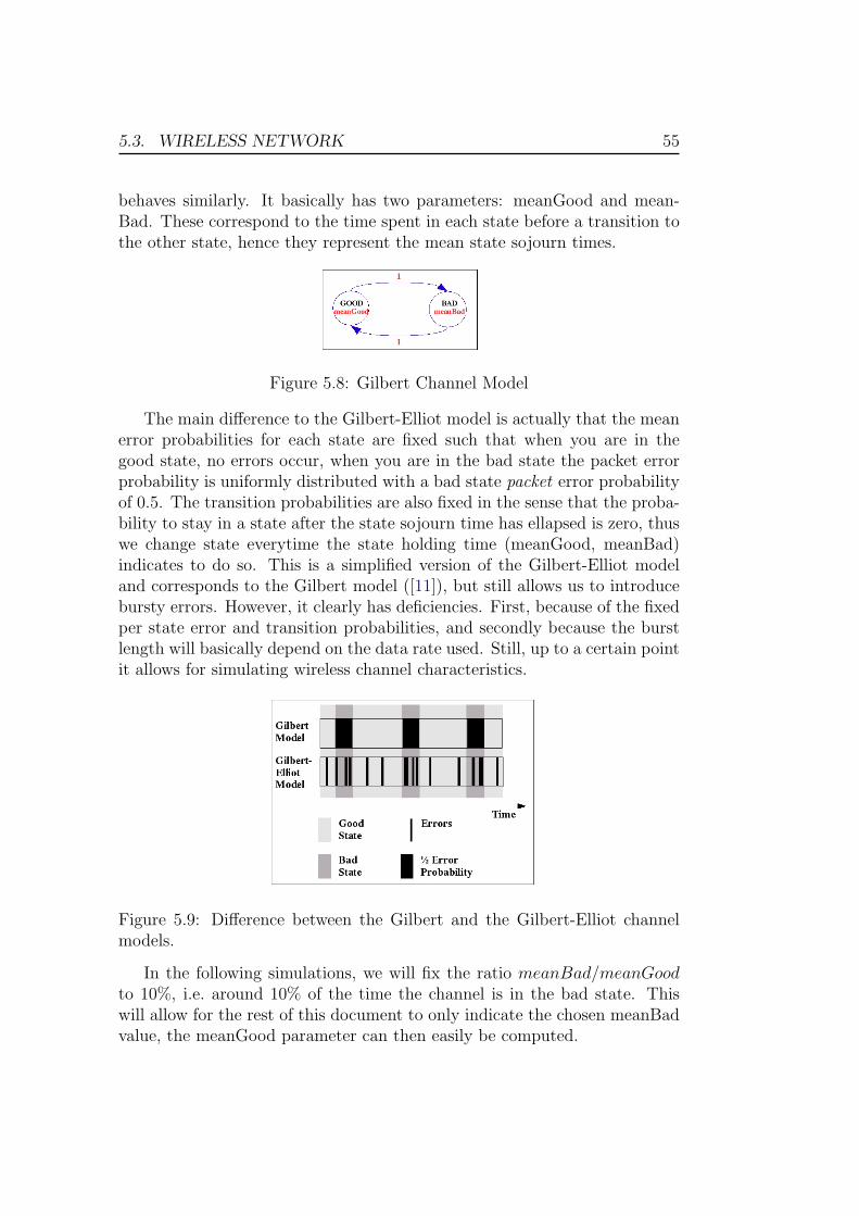
5.3. WIRELESS NETWORK 55

behaves similarly. It basically has two parameters: meanGood and mean-Bad. These correspond to the time spent in each state before a transition tothe other state, hence they represent the mean state sojourn times.

Figure 5.8: Gilbert Channel Model

The main difference to the Gilbert-Elliot model is actually that the meanerror probabilities for each state are fixed such that when you are in thegood state, no errors occur, when you are in the bad state the packet errorprobability is uniformly distributed with a bad state packet error probabilityof 0.5. The transition probabilities are also fixed in the sense that the proba-bility to stay in a state after the state sojourn time has ellapsed is zero, thuswe change state everytime the state holding time (meanGood, meanBad)indicates to do so. This is a simplified version of the Gilbert-Elliot modeland corresponds to the Gilbert model ([11]), but still allows us to introducebursty errors. However, it clearly has deficiencies. First, because of the fixedper state error and transition probabilities, and secondly because the burstlength will basically depend on the data rate used. Still, up to a certain pointit allows for simulating wireless channel characteristics.

Figure 5.9: Difference between the Gilbert and the Gilbert-Elliot channelmodels.

In the following simulations, we will fix the ratio meanBad/meanGoodto 10%, i.e. around 10% of the time the channel is in the bad state. Thiswill allow for the rest of this document to only indicate the chosen meanBadvalue, the meanGood parameter can then easily be computed.


5.3.3 Small IEEE 802.11 Network

We first would like to consider again a simple network of just two clients inaddition to the broker. The bandwidth of the channel is set 2Mb/s and theRTS/CTS mechanism ([20]) is enabled.

As a preliminary step, an adequate sending rate for the publisher shouldbe found. Please note that we reduced the bandwidth of the channel from100Mb/s in the Ethernet network to 2Mb/s. But, also we should considerthat we now have acknowledgments at the MAC layer in addition to thealready existing acknowledgment procedures in TCP and MQTT. Moreover,when RTS/CTS is enabled, we have additional messages sent by the 802.11MAC layer, which should lead to less collisions.

Looking at the end-to-end delay for meanBad values in the range of 0to 60 ms and a small payload size of 30B shows that the impact of varyingthe sending rate is significant. Especially for QoS 2 we see a high variancebetween different sending rates. E.g. decreasing the mean interarrival timefrom 50 to 40ms increases the mean end-to-end delay by at least 2 orders ofmagnitude for higher sojourn times in the bad state of the channel model.Based on these observations, we choose a temporary sending rate of 25 mes-sages/second.

We now would like to see the impact of data load on the performance ofMQTT from the point of view of the end-to-end delay and especially withregard to the b-efficiency.

The focus will be on the mechanisms that actually produce more dataload on the network. There are several features at different protocol levelsthat should be considered. On the MQTT level, we can clearly identify theMQTT payload size as one of the factors contributing to the data load. Also,we expect different QoS levels to be unequally efficient since they producedifferent amounts of MQTT control messages.

At the 802.11 MAC layer, the amount of data sent/received also dependson the fact that the RTS/CTS mechanism is enabled or not. Enabling thiscollision avoidance mechanism leads in general to an increased amount ofdata sent and received. But on the other hand it is supposed to lead to lesscollisions and hence to less retransmissions.

Table 5.12 shows the recorded values for a MQTT payload size of 200B.The results are similar for smaller sized payloads (simulations were performedfor 30B up to 200B of payload). With regard to the mean end-to-end delay,a very obvious observation is made. Since we have only a few hosts (ex-actly 3 of them) sharing the same medium, collisions are quite unlikely tohappen. Hence, the delay introduced by first sending a RTS message andsecondly waiting for the corresponding CTS from the peer before sending


the data frame, clearly affects the end-to-end delay. The higher the QoS,the more significant this impact is since there are more overall packets sent(please note that any MQTT message will trigger the sending of many otherpackets including RTS/CTS frames, MAC layer ACKs, TCP ACKs and even-tually MQTT ACKs). And more (MQTT and TCP) messages sent impliesmore performed RTS/CTS procedures. This also explains why for a disabledRTS/CTS mechanism the mean end-to-end delay for QoS 2 is around threeto four times higher than for lower QoS levels whereas with RTS/CTS theratio is clearly higher (say five to six).

Table 5.12: End-to-end delay [ms] with and without RTS/CTS with 200Bpayload. mB denotes the mean sojourn time in the bad state (= meanBadparameter).

mB [ms] RTS/CTS QoS 0 QoS 1 QoS 2Mean Std. Mean Std. Mean Std.

0

Enabled

6 2 11 5 49 3520 10 31 14 28 71 8040 11 35 16 31 90 16060 12 26 18 35 95 162

0

Disabled

5 1 7 3 23 1120 7 22 10 36 28 2140 8 31 10 30 30 3160 6 28 9 31 35 43

We can also observe how the evolution for different mB (mean bad statesojourn time) differs depending on the usage of RTS/CTS. Having this optiondisabled leads to minor increases in the end-to-end delay. Making usage of theRTS/CTS procedure instead lets the end-to-end delay nearly double whenhaving a 60ms state holding time in the bad state, as compared to havingno additional errors (mB = 0). This is in fact again caused by the increasednumber of steps involved in delivering a MQTT message over TCP and 802.11from sender to receiver, for then it is more probable that a step has to bereexecuted because of a loss. Hence, it shows that in this setup it clearlydoes not pay off to use the RTS/CTS machanism, as it leads to significantlyincreased end-to-end delays because of the additional message flows.

Probably more interesting than the mean end-to-end delay is the efficiencyin terms of bytes sent and received by the MQTT clients. Again we willdiscuss the results for 200B payload, but the observations made also applyfor smaller sized payloads (see figure 5.10). At first, it is interesting to seethat the ratios calculated don’t differ much for different mean bad state so-journ times (that’s why in table 5.13 only the statistics for two mB values


are included). On average they differ by 2 or 3%. It may primarily soundcontradictory to the results obtained for the end-to-end delay. There, weactually experienced quite large variances of the performance for differentmB values, especially for higher QoS levels. However, this can be explainedas follows. First of all we know that for higher mB values the performancedecreases because of retransmissions at any layer (mainly on TCP and onthe MAC layer). Then, the end-to-end delay for a retransmitted packet willmainly depend on the chosen retransmission timeout. But, since retranmit-ted packets will encouter the same mean error probability, the probabilitythat a retransmission is lost is non-negligible. The retransmission timeoutwill then increase exponentially and significantly affect the end-to-end delay.On the other hand, the retransmitted bytes will only add linearly to theb-efficiency ratios, hence the efficiency is less sensitive to retransmissions.

The table also reveals that for a given mB and QoS level with RTS/CTSenabled or disabled, the total amount of bytes sent and received by a clientis independent of the client being a publisher or a subscriber, i.e. Tp and Ts

(see the table) are equal for a given set of parameters. This indicates thatthe clients are in transmission range of each other, because then every packetsent by one client is received by the other, and assuming that both clients arein trasmission range of the broker, they both will receive the brokers data.Moreover, assuming that each PUBLISH message sent by the publisher willbe delivered to the subscriber (TCP should take care of this), the numberof application bytes sent by the publisher equals the number of applicationbytes received by the subscriber. Hence, Tp and Ts are equal.

Table 5.13: B-Efficiency with and without RTS/CTS with 200B payload.Pub denotes the publisher, Sub the subscriber, S the ratio of applicationbytes sent to bytes sent at the MAC layer, R analogously for received bytes.For the publisher Tp refers to the ratio application bytes sent to overall bytessent and received at the MAC layer, for the subscriber analogously withapplication bytes received (Ts).

mB [ms] RTS/CTS QoS 0 QoS 1 QoS 2Pub Sub Pub Sub Pub Sub


0Enabled

.59 .21 .25 .21 .42 .13 .16 .13 .28 .08 .1 .0860 .56 .2 .23 .2 .4 .13 .16 .13 .27 .08 .1 .08

0Disabled

.66 .25 .28 .25 .49 .16 .2 .16 .35 .1 .13 .160 .6 .22 .25 .22 .44 .15 .17 .16 .32 .09 .12 .09

It should now also be clear, why the S ratio is always higher than theR ratio. Again, this is because of the subscriber receiving everything that


0 50 100 150 2000

5

10

15

20

Payload Size [B]

App

l. by

tes/

MA

C b

ytes

sen

t and

rece

ived

[%]

T−Efficiency

0 50 100 150 2000

10

20

30

40

50

60

Payload Size [B]

App

l. by

tes/

MA

C b

ytes

sen

t and

rece

ived

[%]

S−Efficiency

0 50 100 150 2000

5

10

15

20

25

Payload Size [B]

App

l. by

tes/

MA

C b

ytes

sen

t and

rece

ived

[%]

R−Efficiency

QoS 0

QoS 1

QoS 2

QoS 0

QoS 1

QoS 2

QoS 0

QoS 1

QoS 2

Figure 5.10: B-Efficiency for 60ms mean bad state sojourn time and enabledRTS/CTS. T-Efficiency refers to the ratio averaged over Tp and Ts, S- andR-Efficiency denote the S and R ratios.

the publisher sends (to the broker) in addition to the data received from thebroker (be it data sent to the publisher or to the subscriber itself). It isnevertheless impressive to see already with QoS 0 that while for the pub-lisher more than every second byte sent out is MQTT application data, forthe subscriber at most every fourth byte received will be delivered to theapplication. And the higher the QoS, the lower these ratios are, both forthe publisher and for the subscriber. Also, disabling the RTS/CTS mech-anism will not help much, on average we will only see a 5% enhancement.Therefore we can actually state that the RTS/CTS mechanism has ratheran impact on the measured end-to-end delays than on the efficiency ratios(power consumption).

With regard to the Tp and Ts respectively, we see that the lower the QoSlevel, the bigger is the difference of the values between enabled and disabledRTS/CTS mechanism. The reduced number of bytes sent and received isself-explanatory, it corresponds to the RTS/CTS frames that are not sentnor received. Hence, in this setup some power is saved by disabling theRTS/CTS procedure with QoS < 2.

Figure 5.10 summarizes the observations made. It clearly shows that theshape of the different b-efficiency measures is the same for all QoS, whatdiffers is the scale.

5.3.4 Several Publishers and Subscribers

From the observations in the previous section it becomes clear that the factthat clients are in transmission range of each other or not has a clear impacton the performance measures. In the following experiments the clients arerandomly distributed over the test area, some of them being in transmissionrange of each other and some not. In a real life situation it may be possible


to place the clients at adequate positions to reduce the interference, but thisscenario will not be subject of the following simulations.

The network setup is similar to the one in section 5.2.2, i.e. we have 10MQTT publishers and 10 MQTT subscribers subdivided into the same kindsof sets.

Since we have more hosts sharing the medium, it is sensible to increasethe bandwidth to 11Mb/s, which corresponds to a 802.11b network. Simi-larly, the test area has been expanded to 150m · 150m, again because of theincreased number of hosts. This implies that the average distance betweenhosts increases and hence, also the transmission power has been adapted to6mW (∼8dB).

Preliminary tests have shown that already for sending rates of 10 messagesper second (100ms mean interarrival time) per publisher the system becomesvery unstable in the sense that the end-to-end delays rise to tens of secondsand buffers congest. It has to be kept in mind that having 10 publisherssending at such a rate will unevitably lead to an overall sending rate of 100messages per second. This was discovered to be to high already in the setupof the previous section, where we only considered two clients, a publisher anda subscriber. Hence, we will focus on a sending rate of just one message persecond and per publisher. It should however be considered that this will allthe same lead to a highly enough used medium, since all the control messagesof different OSI layers, i.e. RTS/CTS and ACKs at the 802.11 MAC, TCPand MQTT layer, will add to the PUBLISH messages sent.

5.3.4.1 RTS/CTS Enabled

We first consider that the RTS/CTS mechanism is turned on by every MQTThost. Since the sending rate has been reduced, we can effort to increase thepayload sizes and vary them between 200 and 1000B (and we still have aTCP MSS of 536B).

End-to-End Delay

In the following mean end-to-end delay refers to the mean averaged over allclients. We first concentrate on QoS 0 and 1 before discussing the resultsfor QoS 2. The results show that in general increasing the bad state holdingtime of the Gilbert model and thereby increasing the error burstiness of thechannel is not significant for lower application payload sizes. This was alsoobserved in the small network of the previous section. For QoS 0 we actuallyhave a rather smooth evolution of the mean end-to-end delay for differentbad state sojourn times and a fixed paylaod size. Only in the case of 1000B


payload we notice a strong impact of the error burstiness. For QoS 1 weactually see the impact of the burstiness once the payload size goes beyondthe MSS.

Increasing the payload over the MSS threshold leads clearly to an increaseof the mean end-to-end delay as TCP will fragment the payload and hence thefragments of the MQTT PUBLISH message may arrive delayed. However,also for higher payload sizes we have a low variation of the delay for QoS 0(except for the case mentioned above), only the measured delay when havingno additional errors differs significantly. Thus, we have a kind of robustnessagainst error burstiness with QoS 0. This is interesting to compare withthe results we obtained in section 5.3.3 (see table 5.12) where we actuallyexperienced a doubling of the delay when increasing the bad state holdingtime from 0 to 60. This discrepancy basically has two reasons. On one handit is caused by the fact that we have reduced the sending rate. On the otherhand the increased number of clients and the resulting contention periodsand collisions may reduce the impact of additional random packet losses.

Interestingly, QoS 1 seems to be more sensitive to error burstiness when hav-ing big payload sizes. Moreover, the scale of the mean end-to-end delay iscompletely different, we have values around 100% greater than the corre-sponding values for QoS 0. This increase cannot be explained by MQTT’soperation, as the additional PUBACKs in the return paths do not directlydelay the PUBLISH messages to be delivered to the subscribers’ applications.However, it can be explained by the consequences of the additional MQTTPUBACK messages, namely the loading of the medium by the PUBACKsand all the resulting messages (RTS/CTS, 802.11 ACKs, TCP ACKs andpotential retransmissions). In fact, the broker will send a PUBACK for eachPUBLISH received from any of the ten publishers, and the ten subscriberswill do the same when receiving data from the broker. This will obviouslylead to contentions and/or collisions. If we compare these results with theobservations made with Ethernet networks, it shows that a wireless envi-ronment is much more sensitive to additional message traffic, hence we getsignificant differences of the performance between QoS 0 and 1, whereas withEthernet this was not the case.


200 400 600 800 1000

040

80120

0

50

100

150

200

Payload Size [B]

QoS 0

Bad State Sojourn Time [ms]

Mea

n E

nd−t

o−E

nd D

elay

[ms]

200 400 600 800 1000

040

80120

0

100

200

300

400

Payload Size [B]

QoS 1


Mea

n E

nd−t

o−E

nd D

elay

[ms]

Figure 5.11: Mean end-to-end delay evolution for QoS 0 and 1. RTS/CTSenabled.

The most curious results were obtained for QoS 2. As figure 5.12 showswe have tremendous mean end-to-end values in the range of several seconds.It is actually difficult to interpret the results, because there seems to bequite a lot of randomness. Nonetheless, we should take these results as anindication that QoS 2 can lead to unstableness and poor performance ascompared to lower QoS levels. Moreover, it introduces a lot of variance thatmakes it impossible to estimate the performance. It should also be kept inmind that we get such bad results with low sending rates of one message persecond and per publisher, and that we have a simplified network of “only” 20clients. Experimenting with a network of 100 clients or more would probablycompletely break the system, i.e. the effective end-to-end delay would beenormous.

200400

600800

1000

040

80120

0

2

4

6

8

10

Payload Size [B]

QoS 2


Mea

n E

nd−t

o−E

nd D

elay

[s]

Figure 5.12: Mean end-to-end delay evolution for QoS 2. RTS/CTS enabled.

It was mentioned at the beginning of this section that we would also like tocompare the end-to-end delay distributions of different types of subscribers,i.e. clients that are subscribed to different numbers of topics. Nevertheless,comparing the obtained distributions don’t show any particularly interestingbehavior. We would actually expect the distributions to be different when


0 10 20 30 40 50

102

104

106


End

−to−

End

Del

ay [m

s]

End−to−End Delay Distribution for 200B

0 10 20 30 40 50

102

104

106

Simulation Time [sec]E

nd−t

o−E

nd D

elay

[sec

]


Figure 5.13: End-to-end delay distribution with QoS 0. 200 and 1000B.

the higher number of subscribed topics would result in congestions of TCPwindows. But since the contentions and collisions affect all messages equallyand the publishers send at a low rate, there shouldn’t be any special effectwhen being subscribed to more topics.

But what certainly should be compared is the distribution of the end-to-end delay for low and large payload sizes with respect to the MSS. Figure5.13 compares the distribution for payload sizes of 200 and 800B, QoS 0 anda mean bad state holding time of 120ms for a client subscribed to all topics.We observe that actually the peaks reach up to the same values with 200 and800B. But, looking at the bottom line of the plot reveals that there is a larger“base” end-to-end delay for 800B messages. Furthermore, the frequence ofthe peaks is higher with larger payload size, i.e. with 200B peaks are moresporadic.

In figure 5.14 we observe that with QoS 2 there are bursty peaks alreadywith 200B (e.g. during the period between 20 and 30 simulated seconds).Looking at the distribution for 800B, we actually don’t have anymore peaks,we rather have constantly high values. We clearly see the drawback of bigpayload sizes when using QoS 2, and also with lower QoS levels the networkis very sensitive to the payload size.


0 10 20 30 40 50

102

103

104

105

106


End

−to−

End

Del

ay [m

s]


0 10 20 30 40 50102

103

104

105

106


End

−to−

End

Del

ay [s

ec]


Figure 5.14: End-to-end delay distribution with QoS 2. 200 and 1000B.

Since we have seen that the impact of the payload size is huge and weargue that it depends on the MSS, we should consider increasing the MSSto a value beyond the biggest payload size used. Hence, we now will discussthe results for a MSS of 1024B, which is a common value used in mostimplementations.

Figures 5.15 and 5.16 show clearly that by increasing the MSS the meanend-to-end delay was significantly reduced for payload sizes larger than theold MSS. Moreover, for smaller payload sizes we get similar results as with aMSS of 536B. Therefore it seems that although larger packets have a biggerchance to get lost with respect to the random errors introduced, we get muchbetter results if TCP can avoid fragmenting the payload.

However, we again experience a high variance when having QoS 2. More-over, there are no huge mean end-to-end delay values anymore, but still weget significantly larger values than with lower QoS levels due to the natureof QoS 2 (4-way handshake).


0 200 400 600 800 1000

04080120

10

20

30

40

50

60

Payload Size [B]

QoS 0


Mea

n E

nd−t

o−E

nd D

elay

[ms]

0 200 400 600 800 100004080120

20

40

60

80

100

Payload Size [B]

QoS 1


Mea

n E

nd−t

o−E

nd D

elay

[ms]

Figure 5.15: Mean end-to-end delay evolution for QoS 0 and 1 with 1024BMSS. RTS/CTS enabled.

200 400 600 800 1000

040

80120

0.1

0.2

0.3

0.4

0.5

Payload Size [B]

QoS 2


Mea

n E

nd−t

o−E

nd D

elay

[s]

Figure 5.16: Mean end-to-end delay evolution for QoS 2 with 1024B MSS.RTS/CTS enabled.

Efficiency

After having analyzed the measured end-to-end delays, in this section thefocus will be on the (power-)efficiency. Statistics were collected over all pub-lishers on one hand, and over all subscribers on the other hand.

If we first take a look at table 5.14 it seems that introducing bursty errorsvia the Gilbert model does only have an impact on the S and Sm ratios, allthe other values are approximately the same for different mean bad sojourntimes (mB). We can also imagine why the other ratios remain the same. Thenumber of bytes and frames received by any host, both frames addressed tothe receiving host or not (it will receive both and detect on the MAC layerif it is the destination) clearly dominates over the frames sent by a host.That is the reason why e.g. the S and the Tp measures differ by two orders ofmagnitude. In the case of a network of only 2 clients the Tp ratio was clearlyhigher because the publisher only received redundant frames from 2 hosts,


Table 5.14: Efficiency for 200B payload. mB, S, R, Tp and Ts are definedas in table 5.13. Additionally, we have included the ratios with respect tomessages instead of bytes (Sm, Rm, Tpm and Tsm).

mB [ms] QoS 0 QoS 1 QoS 2Pub Sub Pub Sub Pub Sub


0 .58 .005 .03 .04 .41 .003 .024 .023 .26 .002 .014 .013120 .49 .005 .03 .03 .38 .003 .023 .022 .24 .002 .014 .013


0 .24 .002 .01 .01 .12 .0008 .005 .005 .06 .0004 .003 .003120 .18 .001 .009 .009 .1 .0007 .005 .005 .06 .0004 .003 .003

Table 5.15: Efficiency for 1000B payload.



0 .74 .008 .06 .05 .66 .006 .05 .05 .57 .005 .04 .03120 .67 .007 .05 .05 .63 .006 .04 .04 .54 .005 .03 .03


0 .11 .0007 .005 .005 .08 .0005 .004 .003 .05 .0003 .002 .002120 .09 .0006 .004 .004 .07 .0004 .003 .002 .04 .0003 .002 .002

the broker and the other client. In this setup there are 19 other clients, someof them being in transmission range and hence everything sent by them willbe received. In addition, every client will receive everything that the brokersends, since the network setup was chosen in such a way. Hence, if there are20 clients talking to the broker, every client will receive the redundant datasent by the broker to any of the other clients.

Moreover, the measured ratios at message granularity (Sm, Rm, Tpm andTsm) are much smaller than the corresponding byte ratios. This could indi-cate that there are a lot of small frames received by a host. Small framesmay be RTS/CTS and MAC layer ACKs frames. Hence, the radio interfaceis “active” a significant amount of time to receive small control frames, andmost of them are not even being addressed to the host itself.

With 1000B payload, we experience the same robustness against errorsand their burstiness as with smaller payload sizes. If we remember that themean end-to-end delays were significantly influenced by the additional burstyerrors, this is quite astonishing. We can again observe that additional packetlosses due to random errors introduced impact the end-to-end delay, but notvery much the efficiency or wastefulness of the protocol.


In addition, the byte count ratios are eminently higher with 1000B pay-load. Some of them, e.g. the S ratio for QoS 2 are twice as high. However,the price to pay is an increased number of radio interface switches. But thisis clearly due to the overstepping of the MSS. Since TCP will fragment the1000B payload into two packets, the number of frames sent and received willbe higher. And thus, we actually have around 50% lower m-efficiency ratioswith 1000B than with 200B. This is clearly improved when increasing theMSS over 1000B, as table 5.16 shows.

Table 5.16: Efficiency for 1000B payload with 1024B TCP MSS.



0 .86 .01 .07 .07 .76 .008 .06 .06 .62 .006 .04 .04120 .78 .008 .06 .06 .7 .007 .05 .05 .59 .006 .04 .04


0 .24 .002 .01 .01 .12 .0008 .006 .005 .06 .0004 .003 .003120 .19 .001 .009 .008 .1 .0006 .005 .005 .06 .0004 .003 .003

When comparing the ratios between different QoS levels, we notice apretty linear evolution of the values. While we noticed a high variance intro-duced by QoS 2 when discussing the mean end-to-end, this is not true for theefficiency. A reason might be that the end-to-end delay is highly sensitive tocontention periods caused by the additional MQTT control messages. How-ever, the efficiency only depends on the transmission/reception of a frame,not on the time it was delayed because of a busy medium.

5.3.4.2 RTS/CTS Disabled

In this section, the results obtained when disabling the RTS/CTS mechanismare shortly discussed and compared with the results of the previous section.As already mentioned previously, the main benefit of using the RTS/CTSmechanism is when terminals are “hidden” from each other, i.e. they arenot in transmission range of each other, but there is a terminal (in our casethe broker) which both can hear. When having hosts distributed randomlyover the test area, comparisons between results obtained with and withoutRTS/CTS can potentially vary a lot depending on the positioning of thehosts. Since simulations have been carried out with randomly positionedhosts with respect to the broker, the results are of course specific to thatsetup. Therefore, this section should rather serve to give an idea of howsmall or big the difference can be between using and not using RTS/CTS forgiven MQTT and TCP parameters.


End-to-End Delay

Table 5.17 gives an impression of how strong the impact of disabling RTS/CTScan be with regard to the end-to-end delay in a random setup. To have abetter overview, only the results for the smallest and largest payload sizeshave been included.

Clearly, we see a better performance when disabling the RTS/CTS mech-anism for all mB values and both payload sizes. We observed this alreadyin the network with only two MQTT clients in transmission range of eachother. In general it seems that without RTS/CTS we have more stability inseveral dimensions. First, if we look at the variance introduced by the errorburstiness factor mB, the table shows much higher proportional increaseswith RTS/CTS. Secondly, in the dimension of the payload size, it can beidentified that in both cases the impact of having payloads bigger than TCP’sMSS is high. However, it has a deeper effect when enabling RTS/CTS. Third,when increasing the QoS level, we again experience a bigger performance losswith RTS/CTS. So, in summary we cannot find any advantage of using theRTS/CTS mechanism in a network with our parameter settings.

Table 5.17: Mean end-to-end delay [ms] with and without RTS/CTS with200B and 1000B payload.

mB [ms] RTS/CTS QoS 0 QoS 1 QoS 2200B 1000B 200B 1000B 200B 1000B

0

Enabled

13 45 24 82 124 29040 26 117 45 200 230 > 1s80 30 130 50 270 330 > 1s120 30 200 57 400 260 > 1s

0

Disabled

8 23 12 29 49 10040 11 36 17 54 76 77080 11 44 20 62 84 > 1s120 11 42 22 75 86 > 1s

Nevertheless, there is a property that the fact of not using the RTS/CTSmechanism did not solve. With QoS 2 we still have the unstableness whenusing big payload sizes and having additional errors. We get high varianceand mean end-to-end delays in the range of several seconds. This seems tobe an artifact that is difficult to avoid.

In section 5.3.4.1 we determined that also when having a high enoughTCP MSS, i.e. 1024B, we still noticed the high variance of QoS 2 with highpayload sizes when varying the mean bad state sojourn time. Table 5.18compares the measured statistics for 1000B payload and according to the


usage of the RTS/CTS option with the MSS set to 1024B. Again, it showsthat with RTS/CTS the error burstiness affects the measured mean end-to-end delay much more than it is the case when the option is disabled.

Table 5.18: Mean and standard deviation of the end-to-end delay [ms] withand without RTS/CTS with 1000B payload and 1024B MSS.

mB [ms] RTS/CTS QoS 0 QoS 1 QoS 2Mean Std. Mean Std. Mean Std.

0

Enabled

18 11 32 26 150 11040 34 37 58 69 450 36580 36 45 92 138 450 410120 52 84 90 135 280 2740

Disabled

15 6 18 10 62 3540 17 11 29 35 100 8380 17 13 26 20 112 94120 19 18 27 26 170 225

Efficiency

Finally, we will shortly discuss the results for the efficiency of the protocolwithout the usage of RTS/CTS frames. Tables 5.19 to 5.21 contain all thegathered statistics.

As in the case with RTS/CTS, we notice a fairly constant behavior whenincreasing the error burstiness. Comparing the results for no additional errorsand 120ms mean bad state sojourn time evidently points out that except forthe S ratio, no other measure differs by more than 1%. Therefore, accordingto the results and our power consumption estimates, we cannot conclude thathaving larger error burst lengths leads to significantly higher wastefulness ofMQTT. On average, a single publisher will actually experience more TCPor MAC layer retransmissions when having longer error bursts, however thetotal amount of time where the radio interface is not idle, including trans-mission and receiving periods, is fairly constant. This again implies thatthe overall time spent in the receiving state is much longer than the overalltime spent transmitting. Looking up the raw data recorded with OMNeT++shows that for a publisher on average only 8 out of 1000 bytes are transmittedbytes, the rest of the data was received.

What actually interests more is the comparison with the results obtainedwith enabled RTS/CTS option. Comparing the S and Sm ratios makes clearthat sending RTS/CTS frames will actually have an impact on the number


of times the radio switches state. This can be seen by the Sm value that istwice as high with disabled RTS/CTS for all QoS levels. Nonetheless, the Sratio is only 5% higher since RTS/CTS frames are small in size.

It is worth noting that in general it can be detected that the impactof error burstiness on the publisher is bigger with disabled RTS/CTS. E.g.comparing the S ratio for 1000B payload and QoS 1 shows only a 3% decreasewith RTS/CTS enabled when the mean bad state sojourn time is changedfrom 0 to 120ms. But, in the absence of the RTS/CTS mechanism thepublisher will experience a 15% decrease. However, it seems difficult toexplain this behavior. A possible explanation may be that by using RTS/CTSframes, a significant part of the frames sent are exactly frames of that type.Then, an error burst may lead to the loss of RTS/CTS frames and theirretransmissions. And since RTS/CTS frames are small as compared to dataframes, loosing them instead of data frames will not have a deep impact onthe number of MAC layer bytes sent. In the absence of RTS/CTS frames,errors and especially error bursts will affect data frames (or ACKs) and theirretransmissions. So, the probability that the errors will affect frames of biggersize (namely data frames) is actually bigger.


Table 5.19: Efficiency without RTS/CTS and 200B payload.



0 .64 .006 .04 .04 .48 .004 .03 .03 .31 .002 .02 .02120 .54 .005 .03 .03 .39 .003 .02 .02 .27 .002 .01 .01


0 .47 .003 .02 .02 .24 .002 .01 .01 .12 .0008 .006 .005120 .4 .003 .02 .02 .2 .001 .009 .008 .1 .0006 .005 .005

Table 5.20: Efficiency without RTS/CTS and 1000B payload.



0 .79 .009 .06 .06 .73 .008 .05 .05 .6 .006 .04 .04120 .63 .007 .05 .04 .58 .006 .04 .04 .5 .004 .03 .03


0 .23 .001 .01 .01 .16 .001 .007 .007 .09 .0006 .005 .004120 .19 .001 .008 .008 .12 .0007 .005 .005 .08 .0005 .003 .003

Table 5.21: Efficiency without RTS/CTS, 1000B payload and 1024B MSS.



0 89 .01 .07 .07 .79 .09 .06 .06 .66 .007 .05 .05120 .7 .008 .06 .06 .65 .007 .05 .05 .51 .005 .04 .03


0 .47 .003 .02 .02 .24 .002 .01 .01 .1 .0008 .006 .005120 .38 .002 .02 .02 .2 .001 .009 .009 .1 .0006 .004 .004


Chapter 6

Conclusion and Future Work

This chapter is split into two sections: one for the conclusion about thediscrete event simulator OMNeT++, and the other for the MQTT protocolitself.

OMNeT++ as a Simulation Tool

OMNeT++ is definitely worth to be considered a powerful simulation sys-tem that can keep up with other popular simulation tools. Its clear structure,modular design and debugging capabilities are big advantages over other com-mercial and non-commercial simulators. Moreover, its strong GUI supportmakes it one-of-a-kind. With regard to the performance aspect, it seemsthat this represents a big challenge for most popular simulators, and OM-NeT++ is no exception. On the other hand, we face a lack of models andespecially the problem of not enough validated models. This is the reasonwhy in the context of this thesis a TCP and a wireless channel model wereintegrated into the simulator. But considering that the OMNeT++ commu-nity is continuously expanding, it is just a matter of time when more stableand complete simulation models will increasingly satisfy the users needs.

MQTT Performance

In this thesis several performance measures and several factors affecting thesemeasures have been looked at. Of particular interest were the end-to-enddelay and the (power-) efficiency of MQTT. Parameters on several layers(MQTT, TCP, MAC including Ethernet and IEEE 802.11 and physical layer)were varied and the resulting performance observed.

On the basis of a small Ethernet network it was shown how significantlyTCP’s MSS, the timestamp option and the error correlation of the physical

73

74 CHAPTER 6. CONCLUSION AND FUTURE WORK

link affect the measured performance (especially the end-to-end delay). Also,it was demonstrated how higher QoS decrease the efficiency because of theadditional MQTT ACK control messages.

The transition to an Ethernet network with 20 MQTT clients revealedthat when having non-bursty errors we don’t experience significant changesof the performance measures when varying parameters such as the bit errorrate (BER). However, introducing burstiness makes clear how important theBER and the payload size are for the resulting performance. QoS 2 seemsto be a paradoxical case where the end-to-end delay is very sensitive to thevalues of the parameters mentioned above whereas the efficiency stays ratherconstant. It was also shown how the performance for different subscribersvaries depending on the number of topics the clients are subscribed to.

The main focus was however on wireless IEEE 802.11 networks. This com-pletely changes the observed performance since not only we have significantlyhigher probabilities of collisions and contention periods, but also we haveMAC layer acknowledgments. The Gilbert channel model was used to sim-ulate wireless links and the effect of the usage of the RTS/CTS option wastested.

For the network setups tested, much more variance of the end-to-end delaywas observed than in Ethernet networks. Also, the measured performancedifferences between the available QoS levels was eminently higher. In general,the wireless setup proved to be much more sensitive to the parameter settings.With regard to the RTS/CTS mechanism, it was shown that disabling thisoption led to significantly better performance.

Future Work

This project was a first step towards evaluating MQTT’s performance underseveral network assumptions by means of the OMNeT++ simulator. Clearly,testing MQTT under all possible parameter combinations was out of thescope of this work, only a subset of the potential setups has been focused on.For future tests (possibly with OMNeT++ and the MQTT and TCP modelsdeveloped) there are however critical points that should be addressed.

One evident aspect is the network size. In practice, MQTT is used withseveral hundred clients per broker, and this should also be considered inthe simulations. Especially in wireless networks the number of clients playsa crucial role when measuring the performance of the protocol. Neverthe-less, OMNeT++ does not seem to be able to simulate such networks withreasonable performance when using adequate publisher sending rates.

In addition, more tests with different sending rates and distributions

75

would be senseful, as these are important parameters, too.To simulate wireless channels, the Gilbert model shipped with the INET

framework is clearly not sufficient. Another enhanced model should be de-veloped in order to allow for specifying more accurately wireless channelcharacteristics.

The INET framework also provides some support to simulate mobile net-works, i.e. it is possible to have moving hosts. It would be interesting to testMQTT in mobile networks where sensors change position over time. How-ever, this has been identified to lead to more events to be handled by thesimulation kernel and therefore the performance of the simulator degradessignificantly.

76 CHAPTER 6. CONCLUSION AND FUTURE WORK

Bibliography

[1] WebSphere MQ Telemetry Transport.http://publib.boulder.ibm.com/infocenter/wbihelp/index.jsp?topic=/com.ibm.etools.mft.doc/ac10840 .htm

[2] A. Varga. OMNeT++, http://www.omnetpp.org.

[3] K. Entacher, B. Hechenleitner, S. Wegenkittl. A simple OMNeT++queueing experiment using parallel streams. PARALLELNUMERICS’02 - Theory and Applications, pages 89–105, 2002.

[4] P. Hellekalek. Don’t trust parallel Monte Carlo. ACM SIGSIM Simula-tion Digest, 28(1):82–89, July 1998.

[5] Makoto Matsumoto and Takuji Nishimura. Mersenne Twister: A 623-dimensionally equidistributed uniform pseudorandom number generator.ACM Transactions on Modeling and Computer Simulation, 8(1):3–30,1998.

[6] Jeroen Idserda. TCP/IP modeling in OMNeT++. B-Assignment, Uni-versity of Twente, the Netherlands, July 2004.

[7] NetBSD, http://www.netbsd.org.

[8] Roland Bless and Mark Doll. Integration of the FreeBSD TCP/IP-Stackinto the Discrete Event Simulator OMNeT++. Proc. of the 2004 WinterSimulation Conference.

[9] Andreas Willig, Martin Kubisch, Christian Hoene, and Adam Wolisz.Measurements of a Wireless Link in an Industrial Environment using anIEEE 802.11-Compliant Physical Layer. IEEE Transactions on Indus-trial Electronics, 2001.

77

78 BIBLIOGRAPHY

[10] David Eckhard and Peter Steenkiste. Measurement and analysis of theerror characteristics of an in-building wireless network. In Proc. of ACMSIGCOMM’96 Conference, pages 243-254, Stanford University, Califor-nia, August 1996.

[11] E. N. Gilbert. Capacity of a burst-noise channel. Bell Systems TechnicalJournal, 39:1253-1265, September 1960.

[12] E. O. Elliot. Estimates of error rates for codes on burst-noise channels.Bell Systems Technical Journal, 42:1977-1997, September 1963.

[13] Almudena Konrad, Ben Y. Zhao, Anthony D. Joseph, Reiner Ludwig. AMarkov-Based Channel Model Algorithm for Wireless Networks. Wire-less Networks 9, 189-199, 2003.

[14] David D. Clark. Window and Acknowledgment Strategy in TCP. RFC813, July 1982.

[15] V. Jacobson, R. Braden, D. Borman. TCP Extensions for High Perfor-mance. RFC 1323, May 1992.

[16] M. Mathis, J. Mahdavi, S. Floyd, A. Romanow. TCP Selective Acknowl-edgment Options. RFC 2018, October 1996.

[17] J. Postel. TCP Maximum Segment Size and Related Topics. RFC 879,November 1983.

[18] S. Floyd, T. Henderson. The NewReno Modification to TCP’s Fast Re-covery Algorithm. RFC 2582, April 1999.

[19] Kevin Fall and Sally Floyd. Simulation-based Comparisons of Tahoe,Reno, and SACK TCP. Laurence Berkeley National Laboratory.

[20] Wireless LAN Medium Access Control (MAC) and Physical Layer(PHY) Specification. ANSI/IEEE Std 802.11, 1999 Edition (R2003).

[21] Victor Shnayder, Mark Hempstead, Bor-rong Chen, Geoff Werner Allen,and Matt Welsh. Simulating the Power Consumption of a Large-ScaleSensor Network. Harvard University.

Documents

Master’s Thesis · manually input into billing systems to facilitate data transfer. First deployed over 20 years ago, the SCADA architecture has changed very little over time. A