Master thesis

Activity types in a neuralmass model

Jurgen Hebbink

September 19, 2014

Exam committee:Prof. Dr. S.A. van Gils (UT)Dr. H.G.E. Meijer (UT)Dr. G.J.M. Huiskamp (UMC Utrecht)

Contents

1 Introduction 4

2 Neural mass models 62.1 General principle of a neural mass . . . . . . . . . . . . . . . . . . . . . . . . . . 62.2 Lopes da Silva’s thalamus model . . . . . . . . . . . . . . . . . . . . . . . . . . . 82.3 Models for cortical columns . . . . . . . . . . . . . . . . . . . . . . . . . . . . . . 9

2.3.1 Jansen & Rit model . . . . . . . . . . . . . . . . . . . . . . . . . . . . . . 92.3.2 Variations on the Jansen & Rit model . . . . . . . . . . . . . . . . . . . . 10

3 Wendlingmodel 143.1 Model formulation . . . . . . . . . . . . . . . . . . . . . . . . . . . . . . . . . . . 143.2 Activity types . . . . . . . . . . . . . . . . . . . . . . . . . . . . . . . . . . . . . . 16

3.2.1 Activity types found by Wendling et al. . . . . . . . . . . . . . . . . . . . 173.2.2 Other activity types . . . . . . . . . . . . . . . . . . . . . . . . . . . . . . 183.2.3 Variation of synaptic gains . . . . . . . . . . . . . . . . . . . . . . . . . . 23

3.3 Bifurcation analysis in B . . . . . . . . . . . . . . . . . . . . . . . . . . . . . . . . 243.3.1 Continuation in B for G = 25 . . . . . . . . . . . . . . . . . . . . . . . . . 243.3.2 Continuation in B for G = 50 . . . . . . . . . . . . . . . . . . . . . . . . . 28

3.4 Boundaries between equilibrium activity types . . . . . . . . . . . . . . . . . . . 303.5 Activity map for the B-G-plane . . . . . . . . . . . . . . . . . . . . . . . . . . . . 343.6 Continuation of codim 1 bifurcations . . . . . . . . . . . . . . . . . . . . . . . . . 36

4 Conclusion & discussion 39

A Continuation of non-bifurcations 41A.1 Continuation of eigenvalues . . . . . . . . . . . . . . . . . . . . . . . . . . . . . . 41

A.1.1 Continuation of a real eigenvalue . . . . . . . . . . . . . . . . . . . . . . . 41A.1.2 Continuation of a complex conjugated pair of eigenvalues . . . . . . . . . 43

A.2 Limit point at certain value of system variables . . . . . . . . . . . . . . . . . . . 43A.3 Continuation of possible boundaries of activity types . . . . . . . . . . . . . . . . 44

A.3.1 Transition of leading eigenvalue . . . . . . . . . . . . . . . . . . . . . . . . 44A.3.2 Continuation of eigenvalues with a fixed imaginary part . . . . . . . . . . 45

B Simulation source code 46

Bibliography 49

3

Chapter 1

Introduction

Understanding neuronal activity in the human brain is a complex and difficult but necessary taskin order to treat diseases like epilepsy. Due to the complexity there are multiple fields of scienceinvolved. One, at first glance surprising, way to study brain activity is by using mathematicalmodels.

Mathematical models for brain activity are a useful tool because one can study brain activitywithout bothering about effects from outside. Experiments that one can do in a mathematicalmodel are ideal in comparison to real experiments which are always performed under non-idealconditions. Further one can change parameters in mathematical models easy, something thatis difficult or even impossible in real experiments. A drawback of mathematical models is thatthey are always a simplification of the reality. However, a good mathematical model may giveinsight in the underlying processes that generates brain activity.

There are lots of different mathematical models for brain activity. All these models havetheir specific strength and weakness. Some of these models are made to model activity of singleneurons. Often multiple of these single neuron models can be coupled in order to simulate alarge network of neurons. However, one needs lots of coupled neurons to model bigger brainstructures. For example a single cortical column counts in the order of 104-108 neurons [7].

Performing simulations of such large networks of coupled neurons is only feasible on su-percomputers and even then it takes long. Another disadvantage of such big models is thatthey count a huge number of parameters. It’s therefore difficult to analyze the influence of theparameters.

Other classes of mathematical models describe neuronal activity on a macroscopic level.These macroscopic models are less detailed then microscopic models and often describe averageactivity of a large group of neurons. This is not a big problem since most experimental data isthe result of measurements of large groups of neurons. This is for example the case with EEGmeasurements.

An advantage of macroscopic models is that they need less computation time compared tomicroscopic ones. Simulations of macroscopic models can be done on a consumer PC. Furtherthey have significantly less parameters and are therefore easier to analyze. Hence, studyingmacroscopic models may give more insight in brain activity.

In this report we will study a class of macroscopic models that is called Neural Mass Models(NMMs). The basis of NMMs is formed in the seventies by Lopes da Silva et al. [20,21] and byFreeman et al. [9]. In this report we will study a model by Wendling et al. [28] that models thebehaviour of a cortical column. A feature of this model for a cortical column is that it modelstwo different inhibitory processes, a fast and slow one. Most neural mass models for corticalcolumns model only the slow inhibitory process.

The main target of this report will be to investigate the different type of activities that thismodel can generate and what the influence of the two inhibitory processes is on these activitytypes. Another target is to find boundaries between the different activity types we find in this

4

model. This will result in a map that reveals regions where specific activity types are seen.This report is built up in the following way. In the next chapter we start to explain the basic

principle of a neural mass models. After this we give a literature overview of some neural massmodels for cortical columns. In the chapter that follows we investigate the Wendling model inmore detail. First we will formulate a system of differential equations that governs this model.Then we show the different activity types that can be produced by the Wendling model. Thisis followed by bifurcation analysis of the model in one parameter. The bifurcations we find givea part of the boundaries between the activity types. After this we will search how the otherboundaries can be found. It results in an activity map and a bifurcation diagram for a largeparameter region. Finally we will discuss our results in the chapter ’Conclusion & Discussion’.

To this report two appendices are added. In the first appendix is described how the non-bifurcation boundaries between the activity types can be continued using an extended systemof differential equations. The last appendix shows the source code of our implementation of theWendling model in Matlab.

5

Chapter 2

Neural mass models

In this chapter we will discuss neural mass models in more detail. The basic units of neuralmass models are neural masses. A neural mass models the average behaviour of a large group ofneurons. Neural masses are coupled together to model larger structures of neurons like corticalcolumns. Some neural mass models consist of multiple cortical columns that are coupled together.

In this chapter we describe first the general principle of neural mass models and explain howa single neural mass is modeled. Then we discuss one of the first neural mass model namely thatof Lopes da Silva et al. [20]. We finish to comment on some literature on neural mass modelsfor cortical columns.

2.1 General principle of a neural mass

In this section is described how a single neural mass or neural population is modeled. Each neuralmass has average membrane potential, u. This average membrane potential can be viewed as thestate variable of the neural mass. This average membrane potential is the result of the differentinputs that this neural mass receives.

In neural mass models these inputs represents average pulse densities. These inputs can comefrom other neural masses in the model or from external inputs. A neural mass it self can alsogive an output. This output is also an average pulse density.

Average membrane potential and average pulse densities are the two main quantities inneural mass models. These two quantities are converted via two transformations: Post SynapticPotential (PSP) and a potential-to-rate function. Each input to a neural mass is convertedfrom an average pulse density to a potential via a PSP transform. Each of these potentials ismultiplied by some constant, modeling the average number of synapses to this population. Thenthe average membrane potential of a population, u, is formed by summing up all potentials fromexcitatory inputs and subtract all inhibitory ones. The potential-to-rate function converts theaverage membrane potential of a neural mass into the average pulse density that this populationputs out. A schematic overview of a neuronal population is displayed in figure 2.1.

The PSP transformation is a linear transformation and is modeled using a second orderdifferential equation. This second order differential equation is usually characterized in terms ofit’s impulse response. Originally Lopes da Silva et al. [20] approximated the impulse responseof a real PSP by the following impulse response:

h(t) = Q(e−q1t − e−q2t

).

Here Q (in mV) and q1 < q2 (both in Hz) are parameters.Van Rotterdam et al. [27] simplified this approximation by a version that has two parameters,

Q and q. This impulse response is given by:

h(t) =

{Qqte−qt t ≥ 0

0 t < 0. (2.1)

6

−IPSP C2

+EPSP C1

+EPSP C0

u S(u)

Figure 2.1: A schematic overview of a neural mass. Different inputs are converted to potentialsusing PSP transforms. These potentials are multiplied by a constant modeling the averagenumber of synapses from this input to the population. Summing up all excitatory and subtractingall inhibitory potentials yields the average membrane potential u. Then a sigmoid transform isapplied to u in order to get the average pulse rate that this population puts out.

This PSP transformation is used in nearly all later NMMs, for example [10,17,28]. In figure 2.2an example of the impulse response h is plotted. It can be seen that the PSP transform has apeak. The time of this peak can be adjusted by the parameter q, since it lays at t = 1/q. Theother parameter Q is used to tune the height of this peak that is given by Q/e.

The integral of the impulse function h in equation (2.1) is Q/q and depends on both Q and q.From a mathematical point of view one may prefer to tune this with a single variable Q = Q/q.In that case the impulse response becomes.

h(t) =

{Qte−qt t ≥ 0

0 t < 0,

However in this case the maximum height of the peak in the impulse response is Q/(qe) andthis depends on two variables. This could be a reason that van Rotterdam et al. [27] used theimpulse response of equation (2.1). Equation (2.1) has become the standard from then on. Alsowe will use the impulse response described by equation (2.1).

The impulse response in equation (2.1) corresponds to a linear transformation that is givenby the following system of two ODE’s:

dx

dt= y, (2.2a)

dy

dt= Qqz − 2qy − q2x. (2.2b)

Here z(t) is the input to the PSP transform and x(t) the output of the PSP transform.The potential-to-rate function converts the average membrane potential of a population, u,

into an average pulse density. This average pulse density is the output of the neural mass. Thepotential-to-rate function is a non-linear function. It’s usually taken to be a non-decreasingfunction that converges to zero as u→ −∞ and is bounded from above. A common choice is asigmoid function:

S(u) =2e0

1 + er(v0−u), (2.3)

but also other functions are used for example in [18]. In equation (2.3) parameter e0 is half ofthe maximal firing rate of the population, v0 the average membrane potential for which half ofthe population fires and r a parameter for the steepness of the sigmoid. Most times e0 = 2.5Hz,v0 = 6mV and r = 0.56mV−1 are used. A graph of S(u) for these values is plotted in figure 2.3.

With the description of the PSP transform and the potential-to-rate function we have dis-cussed the basic principles that describe the behaviour of a single neural mass. In neural mass

7

h(t)

t1/q

Q/e

O

Figure 2.2: Plot of impulse response function h.

S(v)

vv0

e0

2e0

O

Figure 2.3: Plot of the sigmoid function. It can be seen that for v = v0 the sigmoid function hasa value of e0 and 2e0 is an asymptote.

models multiple neural masses are coupled to model bigger structures. In the next section wediscuss the neural mass model by Lopes da Silva et al. [20] that models the thalamus. Later wewill discuss different models for cortical columns.

2.2 Lopes da Silva’s thalamus model

In 1974 Lopes da Silva et al. [20] published an article where models for the α-rhythm in thethalamus are investigated. In this article a neural network model is reduced to a NMM. Firstthey consider a neural network model that consists of two classes of neurons namely thalamo-cortical relay cells (TCR) and interneurons (IN). Their neural network consists of 144 TCRneurons and 36 IN. With computer simulations is showed that this model is able to produce anα-rhythm.

In order to understand the influence of parameters they reduce this model to a neural massmodel. Their neural mass model consists of two neural masses, one models the TCR, the otherthe IN. The TCR receive external excitatory input and inhibitory input from IN. The IN receiveonly excitatory input from the TCR. In figure 2.4 a schematic overview of this model is given.

The model by Lopes da Silva et al. [20] was adapted in further articles. As mentioned in theprevious section Van Rotterdam et al. [27] proposed the impulse response of PSP transformationin equation (2.1). Let us indicate the parameters for the excitatory PSP with Q = A and q = aand for the inhibitory PSP one Q = B and q = b. Van Rotterdam et al. [27] used A = 3.25mV,a = 100Hz, B = 22mV and b = 50Hz. These values have become the standard in most articles.

8

TCR

Input +

IN

−

+

Figure 2.4: Schematic overview of Lopes da Silva’s NMM for the thalamus. Arrows marked with+ are excitatory connections, with − are inhibitory.

2.3 Models for cortical columns

In this section different neural mass models for cortical columns are discussed. Like the neuralmass model by Lopes da Silva et al. [20] for the thalamus these models couple multiple neuralmasses together. The models for cortical columns that we discuss are based on the model byJansen & Rit [17]. Therefore we will start with a description of this model.

2.3.1 Jansen & Rit model

In 1993 Jansen et al. [18] devolped a model for a cortical column that consist of three neuralmasses: pyramidal neurons, local excitatory and local inhibitory neurons. It was based on themodel for the thalamus by Lopes da Silva et al. [20] and uses the PSP transformation as proposedby van Rotterdam et al. [27].

Two year later, in 1995, Jansen and Rit [17] used a slightly different version of this modelthat is the basis for most cortical NMMs. A schematic representation of this model is showedin figure 2.5. In the Jansen & Rit model pyramidal and local excitatory neurons give excitatoryinput to other populations where local inhibitory neurons give inhibitory input. Local excitatoryand inhibitory neurons both receive input from the pyramidal cells with connectivity strength C1

respectively C3. Pyramidal neurons receive input from both excitatory and inhibitory neuronswith connectivity constants C2 respectively C4.

In the Jansen & Rit model pyramidal cells are the only population that receive externalexcitatory input. This in contrast to the model by Jansen et al. [18]. Here also the localexcitatory cells receive input from outside.

The external input to a cortical column can consist of output from pyramidal cells of othercortical columns and background activity. The model output that is studied is potential ofpyramidal cells, since this is supposed to approximate EEG signals, as pyramidal neurons haveby far the biggest influence on EEG signals.

Pyramidalcells

Input +

Excitatorycells

+, C1

+, C3

Inhibitorycells

−, C4

+, C2

Figure 2.5: Schematic representation of the Jansen & Rit model for a cortical column. Arrowsmarked with + are excitatory connections, with − are inhibitory. The constants Ck, k = 1, 2, 3, 4regulate the strength of the connections.

Jansen and Rit [17] related the connectivity constants in the cortical column by using liter-ature on anatomical data of animals. In this way they found the following relation:

C1 = C, C2 = 0.8C, C3 = C4 = 0.25C, (2.4)

9

with C a parameter. This parameter C is set to 135 in a large part of their work. Furtherthe standard parameters for the sigmoid function are used: e0 = 2.5Hz, r = 0.56mV−1 andv0 = 6mV. As external input Jansen and Rit use noise that varies between 120 to 320Hz

Jansen and Rit [17] vary some parameters. They found out that their model was capable toproduce activity types. These are displayed in figure 2.6. The upper left plot of this figure iswhat they called hyperactive noise. The potential of the pyramidal cells is high for this activitytype. If the inhibition is increased the model produces a noisy α-rhythm and later on a normalα-rhythm. Then slow periodic activity with high amplitudes is seen. If the inhibition is higherthe system produces hypo-active noise. The potential of the pyramidal cells is low in this case.

Wendling et al. [30] used the Jansen-Rit model with Gaussian white noise input with mean90Hz. They claim to use a standard deviation of 30Hz, but probably this is much lower (seechapter 3.1). They observed that for A = 3.25mV the system oscillates in α-rhythm, when A isincreased the model started to create sporadic spikes that become more frequent, till the systemwas only produce spikes.

Grimbert and Faugeras [12] investigated the influence of the stationary input I on the Jansen& Rit model using bifurcation analysis. They used the same parameter values as used by Jansenand Rit. In figure 2.7 the resulting bifurcation diagram is displayed. In this diagram the bluelines represent equilibria and the green lines the maxima and minima of periodic solutions. Solidlines indicate stable solutions and dashed lines unstable.

Grimbert and Faugeras found that the Jansen & Rit model has a large bistable region. For0 < I < 89 the system has 2 stable equilibria. At I ≈ 89 one of these stable equilibria undergoesa Hopf bifurcation. This produces the stable limit cycle that is responsible for the α-rhythm.Between I ≈ 89 and I ≈ 114 the system has a stable equilibrium and the stable limit cycleproducing the α-rhythm. At I ≈ 114 a saddle-node on an invariant curve bifurcation (SNIC)takes place. This bifurcation produces a limit cycle with low frequency (< 5Hz) and the stableequilibrium disappears. The new created limit cycle generates Spike-Wave-Discharge (SWD)activity. Till I ≈ 137 the α-rhythm limit cycle and the SWD limit cycle are the two stablesolutions of the system. At I ≈ 137 the SWD limit cycle disappears because at this point itundergoes a Limit Point of Cycle (LPC) bifurcation with an unstable limit cycle. From thispoint till I ≈ 315 the α-rhythm is the only stable solution of the system. At I ≈ 315 again aHopf bifurcation takes place. The α-rhythm limit cycle disappears and for larger values of I thesystem has a stable equilibrium.

Grimbert and Faugeras [12] also consider briefly changes of other parameters. They concludedthat varying parameters by more then 5% leads to drastic changes in the bifurcation diagram forI. Lower values of A, B and C or higher values of a and b make that the system no longer hasstable limit cyles. Higher values of A, B and C or lower values of a and b give a new bifurcationdiagram. The system is monostable for nearly all values of I and has a broader region (comparedto the standard values) of SWD activity.

2.3.2 Variations on the Jansen & Rit model

In the literature there are a lot of variations on the Jansen & Rit model. In this section weconsider some of these variations.

In 2002 Wendling et al. [28] proposed a modification of the Jansen & Rit model that is ableto produce fast activity that is seen during seizure onset activity in epileptogenic brain regions.Based on bibliographic material they decided to split up the local inhibitory population in a fastand slow population. Therefore this model consists of pyramidal, local excitatory and fast andslow local inhibitory populations, see figure 3.1 on page 14. In this model all local populationreceive excitatory input from the pyramidal cells. The pyramidal cells in their turn receiveexcitatory input from the local excitatory cells and from outside. Further they receive inhibitoryinput from the fast and slow local inhibitory cells. In addition the slow inhibitory cells projectinhibitory input to the fast inhibitory cells. The parameter q of the PSP transform for the fast

10

0 0.5 1 1.5 2

10.5

11

11.5

12

12.5

t (s)

upy(m

V)

Hyperactive noise

0 0.5 1 1.5 2

7.5

8

8.5

9

9.5

10

10.5

t (s)

upy(m

V)

Noisy α-rhythm

0 0.5 1 1.5 2

4

5

6

7

8

9

10

11

t (s)

upy(m

V)

α-rhythm

0 0.5 1 1.5 2

−4

−2

0

2

4

6

8

10

t (s)

upy(m

V)

Slow periodic activity

0 0.5 1 1.5 2

0.5

1

1.5

2

2.5

3

t (s)

upy(m

V)

Hypo-active noise

Figure 2.6: Time series for different activity types seen by Jansen and Rit [17] in their model.Top: hyperactive noise and noisy α-rhythm. Middle: α-rhythm and slow periodic activity.Bottom:hypo-active noise

11

−50 0 50 100 150 200 250 300 350−2

0

2

4

6

8

10

12

LPCSNIC

LP

H H

H

I (Hz)

upy(m

V)

Figure 2.7: Bifurcation diagram of upy as function of I for the Jansen & Rit’s model as obtainedby Grimbert and Faugeras [12].

inhibitory population is very high: q = 500Hz, so the time constant 1/q is very small. This isneeded to produce the fast activity.

More information about the Wendling model can be found in chapter 3. Here we describe theresult found by Wendling et al. [28] and other. Further we will give an overview of the differentactivity types that this model can produce.

A mix of the Jansen & Rit model and the Wendling model is considered by Goodfellow etal. [10]. A schematic overview of this model is given in figure 2.8. Goodfellow’s model has, likethe Jansen & Rit model, three populations. However they modeled a fast and slow inhibitoryconnection from the inhibitory cells to the pyramidal cells instead of only one inhibitory con-nection. Their target is to model the inhibitory process, that according to them has a highlyvariable time course, in a better way. The fast inhibitory PSP taken by Goodfellow et al. [10]uses q = 200Hz and is a lot smaller then in the Wendling model.

Goodfellow et al. [10] developed this model to generate SWD activity in a broad region. Themodel is also capable to produce oscillations with a frequency slightly lower then 15Hz. Theseoscillations are comparable with the α-rhythm in the Jansen & Rit model. Goodfellow et al. [10]call this background activity. Further this model is also able to generate poly SWD (multiplespikes followed by a slow wave) and other complex behaviour.

Pyramidalcells

Input, +

Excitatorycells

+

+

Inhibitorycells

−s

−f

+

Figure 2.8: Schematic representation of Goodfellow’s model [10] of a cortical column.

The model proposed by Goodfellow et al. [10] can be seen as a specific case of a class ofmodels considered by David and Friston [5]. David and Friston generalized the Jansen & Ritmodel as displayed in figure 2.9. Each input to a population is split in n parts. All those partsa processed by their own PSP transformation that have their own parameters. In the figure wehave +1, +2,. . . , +n for the excitatory PSP transforms and −1, −2,. . . ,−n for the inhibitory PSPtransforms. The factor ωk is the fraction of synapses that is processed with PSP transformation

12

k. It holds that:

∀k∈{1,...,n} ωk ≥ 0 andn∑

k=1

ωk = 1.

So the constants C1, C2, C3 and C4 determine the total strength of the connections.

Pyramidalcells

Input +1 +2 +n

Excitatorycells

+1, ω1C1

+2, ω2C1

+n, ωnC1

+1, ω1C3

+2, ω2C3

+n, ωnC3

Inhibitorycells

−1, ω1C4

−2, ω2C4

−n, ωnC4

+1, ω1C2

+2, ω2C2

+n, ωnC2

Figure 2.9: Schematic representation of David and Fristons generalization of the Jansen & Ritmodel.

David & Friston [5] investigate their model for n = 2. They took slow PSP transforms for+1 and −1 and fast PSP transforms for +2 and −2. The other parameters were chosen in suchway that if ω1 = 1 or ω2 = 1 the systems oscillates in a frequency corresponding to the firstresp. second PSP transform under stationary input. If they set (ω1, ω2) = (ω, 1 − ω) and took0 < ω < 1 the system was not oscillating with stationary input. However if a white noise inputwas applied then the started noisy oscillations. The frequency spectrum in those cases didn’thave two separated peaks at the frequencies seen in case ω = 0 or ω = 1 but it had a single peakat some intermediate value, depending on ω.

In this section we discussed several models for a cortical columns. In the next chapter wewill investigate one of them, the Wendling model, in more detail.

13

Chapter 3

Wendlingmodel

In the previous chapter we reviewed different neural mass models for cortical columns. In thischapter we investigate one of them, the model by Wendling et al. [28], in more detail. First aset of differential equations is derived that governs this model. Then is described what types ofactivity this model can produce and what their characteristics are. The next step is to investigatethe influence of inhibition on the activity types. The target is to find boundaries between thedifferent activity types. First this is done by bifurcation analysis. It turns out that not allthe activity types can be separated in this way. Therefore we present a method to find theother boundaries. This leads to a map were different regions of activity are identified. Finallybifurcation analysis in a very broad parameter region is done in order to see what other type ofbehavior this model can produce and from which bifurcations they emerge.

3.1 Model formulation

The model proposed by Wendling et al. [28] consist of 4 neural masses: pyramidal cells, excitatoryinterneurons, slow and fast inhibitory interneurons. In figure 3.1 a schematic overview is given.The pyramidal cells give excitatory input to all other populations. They receive excitatory inputfrom the excitatory cells and from outside. Further they receive slow inhibitory input from theslow inhibitory cells and fast inhibitory input from the fast inhibitory cells. The slow inhibitorycells give also a slow inhibitory input to the fast inhibitory cells.

The signs +, −s and −f along the connectivity arrows in figure 3.1 indicate what parametersfor the PSP transform are used. The + stands for the excitatory PSP transform. The parameters

Pyramidalcells

Input +

Excitatorycells

+, C1

+, C2

Slowinhibitory

cells

+, C3

−s, C4

Fastinhibitory

cells

+, C5

−f , C7

−s, C6

Figure 3.1: Schematic overview of Wendling’s model for a cortical column.

14

Q and q in equation (2.2) for the excitatory PSP are taken to be Q = A and q = a. The sign−s represent the slow inhibitory process. It’s PSP transform has parameters Q = B and q = b.Finally, the −f stands for the fast PSP transform, that has parameters Q = G and q = g.

The parameters Ck, k = 1, . . . , 7 are connectivity constants. It’s useful to express theseconnectivity constants as fraction of a connectivity constant C. We have Ck = αkC, k = 1, . . . , 7,where αk, k = 1, . . . , 7 are parameters that indicate the weight of the connection. The standardvalues for these parameters that are used by Wendling et al. [28] are found in table 3.1. Thesestandard values are the same as those used by Jansen and Rit except for those that are not partof the Jansen & Rit model.

The Wendling model can be described by a set of eight differential equations using thedifferential equations in equation (2.2) that describe the PSP transformation. This leads to thefollowing set of differential equations:

x0 = y0, (3.1a)

y0 = AaS(upy)− 2ay0 − a2x0, (3.1b)

x1 = y1, (3.1c)

y1 = Aa

(I

C2+ S (uex)

)− 2ay1 − a2x1, (3.1d)

x2 = y2, (3.1e)

y2 = BbS (uis)− 2by2 − b2x2, (3.1f)

x3 = y3, (3.1g)

y3 = GgS (uif )− 2gy3 − g2x3, (3.1h)

where

upy = C2x1 − C4x2 − C7x3, uex = C1x0, uis = C3x0, uif = C5x0 − C6x2 (3.2)

are the potentials of the pyramidal cells, excitatory cells, slow inhibitory cells and fast inhibitorycells. The parameter I stands for the external input to the cortical column.

The first two differential equations represent the excitatory input from the pyramidal cellsto the other three populations. Because these three populations process the input from thepyramidal cells with the same PSP transformation this is possible.

The excitatory input to the pyramidal cells consist of excitatory input from the excitatorycells and input from outside the cortical column. These two inputs undergo the same PSPtransformation. After the PSP transformation the potential contribution of the input from theexcitatory cells needs to be multiplied by C2 to account for the number of synapses. For theexternal input there is no multiplication constant needed, since such a constant can be absorbedin the input. After this those two are, together with the potential contribution from the twoinhibitory inputs, added to form the potential of the pyramidal cells.

Because of the linearity of the PSP transformation we can change the order of additionand PSP transformation and the order of multiplication and PSP transform. This leads to thefollowing process. First multiply the input from the excitatory cells with C2. Then add theresult to the external input and apply the PSP transformation. The advantage of this is that weneed to apply the PSP transformation once instead of twice. Therefore we need two differentialequations instead of four to describe the excitatory inputs to the pyramidal cells.

We change this a bit further. We want to apply the multiplication with C2 of the excitatoryinput after the PSP transformation. However, if we do this, we also multiply the potentialcontribution of the external input with C2. To solve this we divide the external input by C2

before the addition. This gives I/C2 term in equation (3.1d). The reason for multiplication afterthe PSP transformation is that the potential of the pyramidal cells, upy, then is given by the

15

formula in equation (3.2). Here all the x’s are multiplied with some Ck which gives a consistentformula.

The fifth and sixth equation model the slow inhibitory input from the slow inhibitory cellsto the pyramidal cells and to the fast inhibitory cells. Finally the last two equations model thefast inhibitory input to the pyramidal cells coming from the fast inhibitory cells.

Note that in most articles where the Wendling model is used [2, 26, 28, 31] the model isdescribed by a set of ten ODE’s. In these systems of ODE’s the slow inhibitory input to thepyramidal cells and to the fast inhibitory cells is modeled by two sets of two ODE’s instead ofone set of two ODE’s.

As mentioned before, the parameter I represents the external input to the cortical column.Usually this input consist of a constant part and a stochastic part. In this chapter we set theconstant part to 90Hz. The stochastic part is modeled as Gaussian white noise. This turnssystem (3.1) into a system of stochastic differential equations (SDE’s).

To solve SDE’s numerically one can’t use methods for ordinary differential equations butadapted methods are needed. For example the Euler-Maruyama method or the Milstein method.Both are based on the plain forward Euler method. The Milstein method includes extra termsin comparison to the Euler-Maruyama method. It therefore has a higher order of strong conver-gence. However for the system of differential equations in (3.1) those two methods are the same,because the coefficient in front of the noise term doesn’t depend on the state variables.

In the articles by Wendling et al. [28, 31] the standard deviation for the white noise is setto σW = 30. However, after trying to reproduce their results this seems way to big. In another article by Wendling et al. [29] a link to the source code that can be used to simulate theWendling model is given. It turns out that they used a plain forward Euler method to simulatethe differential equations. Therefore the actually used standard deviation is:

σ =√

∆tWσW =1√512

30 ≈ 1.33,

where ∆tW is the size of the time step that Wendling at al. [28,31] used. The typical value was1/512s (sampling frequency of 512Hz).

Here we will use σ = 2. This is slightly bigger then the standard deviation used by Wendlinget al. [28] but still acceptable for the system. In the next section we will see what types ofactivity can be generated by the Wendling model.

3.2 Activity types

In their article Wendling et al. [28] distinguished six different types of activity in their system.These six types of activity where found by stochastic simulations of their model for parameters(A,B,G) ∈ [0, 7] × [0, 50] × [0, 30]. They separate these activities based on spectral propertiesand compared this with activity seen in depth-EEG signals.

In this section we first reproduce and describe these six activity types. After this it is showedthat this model is capable to produce also other activity types. Part of these are found byBlenkinsop et al. [2]. We find two new types of activity. One of these is in the region exploredby Wendling et al. [28].

For the simulation of the activity types we made an implementation for the system of differ-ential equations in (3.1). This implementation uses the Euler-Maruyama method to numericallysolve the differential equations and is written in Matlab. The source code can be found inappendix B at page 46.

Besides the time series also the frequency spectra of the different activities are plotted.Due to the noise term in the differential equations these frequency spectra are noisy. One cantry to compute the frequency spectra in absence of noise, but some of the activities are noisyperturbations around a stable equilibrium state and don’t show any activity in absence of noise.

16

Parameter Description Standard value

A Average excitatory synaptic gain 3.25mVB Average slow inhibitory synaptic gain 22mVG Average fast inhibitory synaptic gain 10mV

a Reciprocal of excitatory time constant 100Hzb Reciprocal of slow inhibitory time constant 50Hzg Reciprocal of fast inhibitory time constant 500Hz

C General connectivity constant 135α1 Connectivity: pyramidal to excitatory cells 1α2 Connectivity: excitatory to pyramidal cells 0.8α3 Connectivity: pyramidal to slow inhibitory cells 0.25α4 Connectivity: slow inhibitory to pyramidal cells 0.25α5 Connectivity: pyramidal to fast inhibitory cells 0.3α6 Connectivity: slow to fast inhibitory cells 0.1α7 Connectivity: fast inhibitory to pyramidal cells 0.8

v0 Sigmoid function: potential at half of max firing rate 6mVe0 Sigmoid function: half of max firing rate 2.5Hzr Sigmoid function: steepness parameter 0.56mV−1

Table 3.1: Parameters and their default values as used in the Wendling model.

In order to get smoother frequency spectra we simulated (n+1)10s of model data. We neglectedthe first 10s of the output, in order to remove the effect of initial conditions. The other part isdivided in n parts of 10s. For each part we computed the frequency spectrum after subtractingthe mean. Then we averaged the results. The number of averaged parts, n, depends on the typeof activity.

3.2.1 Activity types found by Wendling et al.

We now reproduce the activity types found by Wendling et al. [28] and try to give a cleardescription. We set A = 5 and varied B and G. The other parameters are set at their standardvalues as displayed in table 3.1. In figure 3.2 examples of the first four types of activity are givenand in figure 3.3 the other two types of activity are given.

The activity that is called type 1 activity by Wendling et al. [28] is shown in the upper leftplot of figure 3.2. This plot is made for (B,G) = (50, 15) and for the frequency plot n = 500 isused. The activity can be described as a noisy perturbation around an equilibrium, because inabsence of noise the system goes to an equilibrium. The frequency plot has a maximum around5Hz. The power of this maximum is low because the activity is noise-driven. According to [28]this represents normal background activity.

Wendling et al. [28] don’t mention that this activity type can be divided in two sub activitytypes depending on the mean value of upy. We call type 1 activity type 1a if upy is low (say < 2)and type 1b if upy is high (say > 10). There is no type 1 activity seen for mid values of upy.In case of type 1a activity the system is nearly inactive, all populations have a relatively lowpotential and therefore the pulse rate they send to each other is low. In case we have type 1bactivity the system is almost saturated, most populations have a relatively high potential andtherefore the pulse rate they send is high. There spectral properties of these subtypes are nearlyequal.

Type 2 activity represents normal activity with sporadic spikes. It can be seen as type 1activity with Spikes Wave Discharges (SWD) appearing now and then. The rate at which theseSWDs appear depends on parameter values and also the standard deviation of the noise. Theplot in figure 3.2 is made for (B,G) = (40, 15). For the frequency plot n = 1000 is used. This

17

frequency plot shows a peak around 3Hz which is caused by the SWDs. Around 5Hz the decayof this peak show some irregularity. This is the effect of the period with normal activity.

The activity called type 3 consist of sustained SWDs. These SWDs are not very sensible fornoise. This is because they are not generated by noisy perturbations around an equilibrium butby a limit cycle with large amplitude. This can also be seen in the frequency plot that shows asharp peak with a high power around 4.5Hz. Other peaks are seen at multiples 2, 3 and 4 of thisfrequency. These higher harmonics arise because the limit cycle isn’t a sinus-like oscillation. Thefrequency of the SWDs changes on parameter variation, the maximum frequency of the SWDsis roughly 5Hz. The example showed in figure 3.2 uses (B,G) = (25, 15). For the frequency plotonly 10 averages were needed.

Activity type 4 distinguished by Wendling et al. [28] is what they call slow rhythmic activity.As can be seen in figure 3.2, which uses (B,G) = (10, 15), this activity shows some very noisyoscillations with highly varying amplitude. This is because the oscillations are noise-driven,in absence of noise the system goes to a stable equilibrium. The frequency of the oscillationschanges a bit on parameter variation but lays around 10Hz as can be seen in the frequency plotthat needed 200 averages.

An example of activity type 5 is given in the upper plot of figure 3.3. For this example weused (B,G) = (5, 25) and n = 500. This activity is called low-voltage rapid activity by Wendlinget al. [28]. As one can see in the plot, this type of activity features relatively irregular fluctuationswith low amplitude, compared to the other activity types. The fact that the fluctuations havea low amplitude comes from the fact that this activity type is caused by stochastic fluctuationsaround an equilibrium state. This can also be seen in the frequency plot, because the maximumpower that is observed is very low. A more interesting thing that can be seen in the frequencyspectrum is that it has two local maxima. The first one appears at a very low frequency andis the result of noise. The second one is in the range 13-25Hz. Between those two maxima thepower is relatively high, this makes that there is a broad frequency region with approximatelythe same power. In this activity type the influence of frequencies around 20Hz is relatively large,this is probably the reason why it’s called rapid activity by Wendling et al. [28]. However, as wewill see later, this model is also capable to produce activities with higher frequencies.

The last activity type distinguished by Wendling et al. [28] is activity type 6. In figure 3.3an example of this activity type is displayed using (B,G) = (15, 0) and only 10 averages for thefrequency plot. Wendling et al. [28] call this slow quasi-sinusoidal activity. This activity consistof oscillations that have a high amplitude that is varying a bit. These small variations are effectsof noise. In absence of noise this activity converges to a stable limit cycle and therefore producesoscillations that all have the same amplitude. The frequency of these oscillations is around 11Hzas the peak in the frequency plot indicates.

There are some relations between these activity types. Sometimes this makes it difficult toclassify the right activity type. Type 4 and type 6 both show oscillations with a frequency around10Hz. The criteria we will use is that type 4 activity is generated by random perturbations aroundan equilibrium state while type 6 is generated by a limit cycle. Further type 2 can be seen as amixture of type 1 and type 3. It’s difficult to formulate a clear boundary between those types.It depends on what you will call a ’sporadic spike’ and is influenced by the standard deviationof the noise. In one of the next sections bifurcation analysis is done and based on this this wetry to define the boundary between these types. However, first it is shown that also other typesof activity can be found in the Wendling model.

3.2.2 Other activity types

Besides the six activity types found by Wendling et al. [28] there are also other types of activitypresent in this model. In [2] is showed that this model is capable to produce different types ofpoly SWD (pSWD) for high values of A and G that lay outside the region exploit by Wendlinget al [28]. In figure 3.4 two different pSWD activities are shown. The first one has 2 spikes

18

0 0.5 1 1.5 2

−3

−2

−1

0

1

t (s)

upy(m

V)

Type 1 activity

0 20 400

0.02

0.04

0.06

0.08

f (Hz)

pow

er0 0.5 1 1.5 2

−20

−10

0

10

20

t (s)

upy(m

V)

Type 2 activity

0 20 400

0.2

0.4

0.6

0.8

f (Hz)pow

er

0 0.5 1 1.5 2

−10

−5

0

5

10

15

t (s)

upy(m

V)

Type 3 activity

0 20 400

1

2

3

4

5

f (Hz)

pow

er

0 0.5 1 1.5 2

7

8

9

10

11

t (s)

upy(m

V)

Type 4 activity

0 20 400

0.02

0.04

0.06

0.08

0.1

f (Hz)

pow

er

Figure 3.2: From above to bottom activity types 1 to 4. Left: typical time series. Right:frequency plot.

19

0 0.5 1 1.5 2

9

10

11

12

13

t (s)

upy(m

V)

Type 5 activity

0 20 400

0.01

0.02

0.03

0.04

f (Hz)

pow

er

0 0.5 1 1.5 2

0

5

10

15

t (s)

upy(m

V)

Type 6 activity

0 20 400

1

2

3

f (Hz)

pow

er

Figure 3.3: From above to bottom activity types 5 and 6. Left: typical time series. Right:frequency plot.

20

0 0.5 1 1.5 2

−20

−10

0

10

20

t (s)

upy(m

V)

pSWD 2 spikes

0 20 400

2

4

6

f (Hz)

pow

er

0 0.5 1 1.5 2

−10

0

10

20

t (s)

upy(m

V)

pSWD 3 spikes

0 20 400

1

2

3

4

f (Hz)

pow

erFigure 3.4: Two examples of pSWD activityies found by Blenkinsop et al. [2]. Top: 2 spikes,bottom: 3 spikes. Left: typical time series. Right: frequency plot.

followed by a wave. For this plot we used A = 7, B = 30 and G = 50. The other one has3 spikes followed by a wave. For the example plot in figure 3.4 we used A = 7, B = 25 andG = 150. Both frequency plots are obtained with n = 10 and look like the frequency plot of theplain SWD case. Like the SWD activity also the pSWD activity is generated by a limit cycle.Besides the pSWD activity type Blenkinsop et al. [2] note that system is able to very complextypes of activity in certain parameter ranges. According to them a lot of these activity typesresemble wave forms that are seen in EEGs.

Neither considered in by Wendling et al. [28] nor by Blenkinsop et al. [2] are oscillations witha frequency of around 30-35Hz. These oscillations come in two different types of activity. Theactivity that we will call type 7 is displayed in the upper plot of figure 3.5. This activity canbe compared to activity type 4. It are noisy oscillation that vary a lot in amplitude and have afrequency that is around 30Hz. The oscillations are noise-driven, because in absence of noise thissystem converges to an equilibrium. This activity type exists in a small part of the parameterregion that is exploit by [28]. It uses a high value of G and a low value of B. For the plots infigure 3.5 A = 5, B = 0 and G = 30 is used. For the frequency plot 200 averages were needed.

The activity type that we will call type 8 is plotted in the lower plot of figure 3.5. For thisexample we used A = 5, B = 0, G = 45 and n = 10. In general this type of activity is visiblefor low values of B and values of G that are a bit bigger then those considered by Wendlinget al. [28]. This activity can be compared with activity type 6 of Wendling et al. [28]. It is anoscillation with a relatively high amplitude that varies a small bit due to the noise. In absenceof noise the system converges to a stable limit cycle with frequency 35Hz.

21

0 0.5 1 1.5 2

7

7.5

8

8.5

9

9.5

t (s)

upy(m

V)

Type 7 activity

0 20 400

0.01

0.02

0.03

0.04

0.05

f (Hz)

pow

er

0 0.5 1 1.5 2

0

5

10

15

t (s)

upy(m

V)

Type 8 activity

0 20 400

0.5

1

1.5

2

2.5

f (Hz)

pow

er

Figure 3.5: From above to bottom activity types 7 and 8. Left: typical time series. Right:frequency plot.

22

Figure 3.6: Activity maps, made by Wendling et al. [28], of the B-G-plane for A = 3.5 (left) andA = 5 (right). Type 1: blue, type 2: cyan, type 3: green, type 4: yellow, type 5: red and type6: white. Images taken from [28].

3.2.3 Variation of synaptic gains

Based on their classification of activity types Wendling et al. [28] explored the activity typesseen in the B-G-plane for various values of A by doing simulations for different parameter values.In this procedure parameter A was varied between 3 and 7 with stepsize 0.5. They varied Band G with a resolution of 1mV between 0 and 50 resp. 0 and 30. For every simulation theydetermined the activity type by looking at the frequency spectrum. In this way they obtained acolour map as displayed figure 3.6.

The colour maps in figure 3.6 are for the cases A = 3.5 and A = 5 those two are representativefor the other maps. In both cases there are two regions of type 1 activity (blue). It turns outthat the type 1 region at the lower left corner is type 1b and the region at the right is is type 1a.

The case A = 3.5 is representative for the activity maps for A ≤ 4. In these maps there is noor a small region of type 2 activity (sporadic spikes, cyan) and type 3 activity (sustained SWD’s,green). According to Wendling et al. [28] is the transition, that is seen if the border from thetype 1b region (blue) to the type 4 region (yellow) is crossed, typically seen during ictal periodsin brain regions that don’t belong to the epileptic zone. A further property of the activity mapsfor low A is that it contains a small type 5 activity region. In case A = 3 this activity type isn’teven visible.

The case A = 5 is representative for the activity maps seen for A > 4. It contains all theactivity types that Wendling et al. [28] distinguished. The region with type 3 activity grows tothe right (higher values of B) if A gets bigger. This causes also that the region of type 2 activityshifts to the right if A is increased, but the area of this region stays approximately equal. Furtherit can be seen that the type 5 region (rapid activity) grows.

Because Wendling et al. [28] did distinguish only six types of activity their maps don’t containactivity type 7 that is visible in a small part of the region they explored. The example in figure3.5 is also made for parameters that in this region. Type 7 is seen in the upper left corner of thered regions found by Wendling.

There are further differences between the activity maps of Wendling and the activity typeswe observe with our model. This is probably because the definition of the activity types weuse here, is different from that used by Wendling et al. [28]. As far as it is clear from [28] theyuse only spectral properties. Our formulation of the activity types uses also the behavior understationary input I.

In the next section we do bifurcation analysis on the Wendling model. We will use the resultsto find the boundaries between the activity types in the B-G-plane.

23

0 10 20 30 40 50 60 70

−15

−10

−5

0

5

10

15

B (mV)

upy(m

V)

H

LP

LP

IP

Hom

Figure 3.7: Bifurcation diagram of uPY for continuation in B. Here we fixed G = 25 and I = 90.Blue lines indicate equilibria. Green lines indicate the minima and maxima of the limit cycle.The cyan lines indicate the local minima and maxima of the limit cycle that arises through theexistence of spikes. Solid lines stand for stable solutions and dashed lines for unstable ones.

3.3 Bifurcation analysis in B

In this section bifurcation analysis on the Wendling model is performed. With the results we getmore insight in the behaviour of the Wendling model under stationary input. It is also useful forfinding the boundaries of the activity types for the model with white noise input. Bifurcationanalysis on the Wendling model is done before by [2,26]. In [26] the focus is on continuation of Iand C. Like [2] we will do continuation in B and G. We will find some new curves and give somenew interpretations. Our focus will be at separating the different types of activity including thenew types 7 and 8.

The bifurcation analysis is done using Matcont [8]. This is a package for numerical contin-uation in Matlab. During the bifurcation analysis A is fixed at A = 5 because for this valuemost types of activity can be seen. Further, it’s assumed that the input I is constant with valueI = 90, the mean value that is used if white noise is added.

In this section we will do bifurcation analysis in B while G is fixed at G = 25 or G = 50. Thisgives a part of the boundaries between the activities. It turns out that the others boundariesare no bifurcations. In the next section we present a new way to determine them.

3.3.1 Continuation in B for G = 25

Based on the activity map made by Wendling et al. [28] for A = 5 (see figure 3.6) we decided todo bifurcation analysis in B with G fixed at G = 25. This is done because this bifurcation curvewill cross regions of different activity types.

In figure 3.7 we see what happens to uPY if B is varied. Equilibria are indicated in blue. Asolid line means that the equilibrium is stable and a dashed line means that the equilibrium isunstable. We see that for low values of B we have a stable equilibrium. At B ≈ 13.08 a Hopfbifurcation takes place and the equilibrium gets two unstable eigenvalues. For B ≈ 64.42 a limitpoint bifurcation takes place. At this point the curve turns ’backwards’. From there on theequilibrium has one unstable eigenvalue up to the second limit point that is found at B ≈ 37.66.From here on the equilibrium point is stable again.

From the Hopf point a limit cycle can be continued. Because the Lyapunov coefficient

24

0 0.02 0.04 0.06 0.08

4

6

8

10

12

t (s)

upy(m

V)

0 0.05 0.1

2

4

6

8

10

12

t (s)

upy(m

V)

0 0.05 0.1 0.15

2

4

6

8

10

12

t (s)

upy(m

V)

0 0.1 0.2

2

4

6

8

10

12

t (s)

upy(m

V)

0 0.1 0.2

0

5

10

t (s)

upy(m

V)

0 0.5 1 1.5

−5

0

5

10

t (s)upy(m

V)

Figure 3.8: Plot of limit cycles, upy against time, for different values of B. Top row: B = 16.0,B = 19.5 and B = 20.4. Bottom row: B = 20.8, B = 25.0 and B = 37.7. Parameters A and Gare fixed at A = 5 and G = 25.

of the Hopf point is negative a stable limit cycle will appear in the direction of the unstableequilibrium branch. In the bifurcation plot 3.7 the minima and maxima in uPY of this limitcycle are indicated by the green curves. The magenta curves show local minima and maxima ofthe limit cycle.

Right after the Hopf bifurcation the time profile of the limit cycle has the shape of a sinus-like oscillation as can be seen in the upper left plot of figure 3.8. Therefore the limit cycle hasa single minimum and maximum. The period of this oscillation is around 80 to 100ms whichmeans that the frequency is between 10 to 12Hz. This can also be seen in figure 3.9, where thefrequency of the limit cycle is plotted against B.

In the bifurcation plot (figure 3.7) it can be seen that at B ≈ 19.54 a special point is markedwith IP. At this point the limit cycle has an inflection point in uPY as can be seen in the timeprofile of the limit cycle in the upper center plot of figure 3.8. This limit cycle has a point wherethe first and second derivative of upy in time are zero, which means that the limit cycle has aninflection point. One can also observe in figure 3.9 that the frequency of the limit cycle goesdown around the inflection point to approximately 5Hz.

An inflection point that appears in a limit cycle is not a bifurcation. At a bifurcation pointthe phase portrait of the dynamical system changes topologically [19]. This is not the case atan inflection point. A consequence of this is that the stability of the limit cycle isn’t changed,the limit cycle remains stable after the bifurcation point.

However, what does change at the inflection point is our interpretation of the behavior of

25

the limit cycle. For values of B beyond the inflection point the limit cycle has two local minimaand maxima instead of a single minimum and maximum. Hence, the geometry of the limit cyclehas changed.

Due to this new minimum and maximum a spike is born. A spike is sharp positive deflectionwith a duration of 20-80ms [25]. In the upper right plot of figure 3.8 we see that there exista sharp positive deflection between the global minimum and the local minimum (keep in mindthat the y-axis is reversed as is usual for EEG signals). After this positive deflection upy goesdown till the local minimum is reached. After this the limit cycle continues his slow wave. Inthe bifurcation diagram 3.7 we indicated the maximum of the spike (local maximum) by a cyanline. Also the local minimum that exist due to the spike is indicated by a cyan line.

The non-global minimum decreases as B increases and at a given point it is as low as theglobal minimum. The limit cycle has two global minima as is displayed in the lower left plot offigure 3.8. After this point the non-global minimum switches to the other hole of the limit cycle.This gives the corner in the cyan line in the bifurcation diagram (figure 3.7).

If B goes up further the frequency of the limit cycle goes down to zero (see figure 3.9)or equivalently the period goes up to infinity. This is because the limit cycle approaches ahomoclinic bifurcation. At this point the limit cycle becomes a homoclinic orbit and disappearsfor larger values of B. This homoclinic bifurcation takes place directly after the second limitpoint bifurcation of the equilibrium. For G = 25 these bifurcations don’t fall exactly together sothere is a region where both the limit cycle and an equilibrium point are stable. This region isvery small, the difference in B value is less then 0.01. Therefore this region is not physiologicallyrelevant. Later we shall see that there are larger values of G where the limit point and homoclinicbifurcation fall together and we have a so called Saddle-Node on an Invariant Curve (SNIC)bifurcation.

If we inspect the bifurcation diagram in figure 3.7 again we see that we now have describedall bifurcations and curves. Therefore we will now give an interpretation of these results andcompare them to the activity map of Wendling et al. [28] in figure 3.6. For low values of B thebifurcation diagram shows that the system has a stable equilibrium. This agrees with the factthat in Wendlings map activity type 4 and 5 are seen. Both these activity types arise from astable equilibrium. The boundary between those two regions is not a bifurcation.

The Hopf point we found is the transition from a stable equilibrium to a stable limit cycle.In the definition we have given only type 3 (SWDs) and type 6 (α-rhythm oscillations) arisefrom a stable limit cycle. From the investigation of the limit cycle it turns out that right afterthe Hopf point type 6 is present and later on type 3 is seen. They are separated by the inflectionpoint we found.

However if we compare this with Wendling’s activity map (figure 3.6) we don’t see activitytype 6 for G = 25 but a direct transition from type 4 to type 3. This can be explained by thefact that type 4 and type 6 are closely related to each other. Type 4 consist of noise-drivenoscillation with a frequency that is near to that of the limit cycle that causes type 6 activity. It’splausible that Wendling et al. [28] classified this as type 4 activity. Unfortunately, they don’tgive an explicit definition of their activity types, so we can’t check this.

Further we found a homoclinic bifurcation of the limit cycle and a limit point bifurcation ofthe equilibrium that where close together. This can be seen as the transition between type 3 andan equilibrium activity type. Comparing with figure 3.6, which shows Wendling’s activity map,it turns out that this must be the transition to type 1 activity. More precise it follows from thebifurcation diagram that the equilibrium value of upy is low, so it is type 1a activity.

In Wendling’s activity map the transition from type 3 to type 1 goes via type 2 activity. Asindicated before, type 2 activity is a mix between type 1 and 3 and may come from a bistableregion. However the bistable region we found in the bifurcation diagram is to small to explainthe width of the type 2 activity region. A good reason for this can be the fact that for thebifurcation analysis the input I = 90 is constant while Wendling et al. [28] used Gaussian noise

26

15 20 25 30 35

2

4

6

8

10

12

B (mV)

fLC(H

z)

Figure 3.9: Plot of frequency of the limit cycleas function of B.

0 10 20 30 4080

85

90

95

100

NCH

B (mV)

I(H

z)

Figure 3.10: Bifurcation diagram in B and I.Blue: limit point, red: Hopf, orange: inflec-tion point. Horizontal lines indicate I = 84,I = 90 and I = 96. Vertical lines indicate theboundaries for which the blue line lays betweenI = 84 and I = 96.

input with mean µ = 90. It therefore interesting to see what happens to the bifurcation pointsif I is varied, but still assumed to be constant.

In figure 3.10 the continuation of the Hopf point, inflection point and limit point in B andI is shown. One can see that the B value for which the Hopf bifurcation takes place almoststays constant if I varies. The same holds for the inflection point. This in contrast to the Bvalue of the limit point. This is more sensitive to changes in I. The homoclinic bifurcationchanges in the same way as the limit point bifurcation. Those two points stay close together. AtI ≈ 87.2 Matcont detects a Non-Central Homoclinic bifurcation, indicated with NCH in figure3.10. At this point the homoclinic curve gets ’glued’ to the limit point curve and they continueas a Saddle-Node on an Invariant Curve (SNIC) for lower values of I.

The curves in figure 3.10 divide the B-I-plane in a number of regions. In the region leftof the Hopf curve (red line) the system has a stable equilibrium. Between the Hopf line andinflection point line (orange) the system has a stable limit cycle that looks like an α-rhythmoscillation. Between the inflection point line and the limit point line (blue) the system has theSWD limit cycle. Finally, right of the limit point line (and also right of the homoclinic curvethat lies approximately on the limit point curve) the system has a stable equilibrium again.

It’s known that about 99% of the Gaussian distribution lies between µ− 3σ and µ+ 3σ. Infigure 3.10 these lines are indicated as horizontal black dash-dotted lines while the horizontalblack dashed line indicates the mean value, I = 90. The two vertical black lines indicate thevalues B ≈ 35.65 and B ≈ 39.74. Between these values of B the limit point curve lays insidethe zone I = µ ± 3σ. In this zone the system can jump from the SWD activity to equilibriumactivity by varying I between µ± 3σ. Hence in this region we can expect to see sporadic spikeactivity (type 2) if the system is perturbed with white noise.

One has to note that the bifurcation curves in figure 3.10 are valid for stationary values ofI and don’t tell exactly what happens if I varies as white noise. However it will give someindication where we can expect that due to the noise the system switches between SWD activityand fluctuation around a stable equilibrium. We therefore take the limit points for I = µ ± 3σas boundaries between type 1 and type 2 resp. type 2 and type 3 activity.

In this section we saw that for G = 25 we were able to find the boundaries between most of

27

the activity types. The only boundary that isn’t found is the boundary between type 5 and type4. This is because both activity arise from noise-driven perturbation around an equilibrium andthe transition between those two is no bifurcation.

This holds for all boundaries between activity types that are noise-driven perturbationsaround an equilibrium (i.e. boundaries between type 1a, 4 and 5). If one wants to find boundariesbetween these types one need to find another method. This will be done in a later section.

First is looked at the bifurcation diagram for B with G fixed at G = 50, because it turnsout that for this value of G the model has an interesting bifurcation diagram. The bifurcationdiagrams for B with G fixed at a value lower then 25 are qualitatively the same as the bifurcationdiagram in figure 3.7 and are therefore less interesting.

3.3.2 Continuation in B for G = 50

In this subsection bifurcation analysis in B is done while G is fixed at G = 50. In figure 3.11 theresult of the bifurcation analysis is shown. The blue line in this figure indicate the value of upyat an equilibrium point. A solid line indicates a stable solution and a dashed line an unstableone.

In contrast to the case G = 25 there is no stable equilibrium for low values of B. At B ≈ 4.13the equilibrium undergoes a Hopf bifurcation and becomes stable. The rest of the bifurcationdiagram for the equilibrium point is qualitatively the same as in the caseG = 25. The equilibriumhas another Hopf bifurcation at B ≈ 14.19 and becomes unstable. At B ≈ 64.31 the equilibriumhas a limit point. The equilibrium curve turns ’backward’. At B ≈ 34.81 the equilibriumundergoes a SNIC bifurcation. The equilibrium becomes stable again and this remains the casefor higher values of B.

From the Hopf point at B ≈ 4.13 a stable limit cycle bifurcates in the direction of theunstable equilibrium. The minima and maxima of this limit cycle are shown by the green linesin figure 3.11. This limit cycle has the shape of a sinus-like oscillation and has a frequency ofapproximately 35Hz.

From the other Hopf point at B ≈ 14.19 also a stable limit cycle bifurcates. Like in the caseG = 25 this limit cycle shows first a sinus-like oscillation with a frequency in the α-band. Adifference with the case G = 25 is that this limit cycle undergoes a period doubling bifurcation atG ≈ 21.53. Here the limit cycle becomes unstable (see lower plot of figure 3.11). This unstablelimit cycle has two inflection points, the first at B ≈ 22.4 and the second at B ≈ 23.72. Afterthe second inflection point the limit cycle has 3 local minima and maxima. This limit cycle hasa wave shape that can be seen as pSWD activity, it has two spikes followed by a wave.

The second inflection point is quickly followed by a period doubling at B ≈ 23.75. After thispoint the limit cycle becomes stable for a short time, because at B ≈ 23.8 the limit cycle hasa limit point of cycle bifurcation. The curve of limit cycles turns ’backwards’. At B ≈ 23.52 asecond limit point of cycles is detected. The limit cycle becomes stable and the limit cycle curveturns ’forward’ again. The stable limit cycle has another inflection point at B ≈ 27.29. At thisinflection point one local minimum and maximum disappears. After this inflection point thelimit cycle has a SWD shape. This SWD limit cycle disappears at the SNIC point at B ≈ 34.81.

From the period doubling points it’s possible to continue a stable limit cycle with doubleperiod (not shown in figure 3.11). This limit cycle has a period doubling bifurcation quicklyafter it’s birth and it becomes unstable. It’s possible to continue an other limit cycle withdouble period (w.r.t the double period limit cycle) from this point. To continue this limit cyclenumerically one need to increase the accuracy of the continuation. This is possible but the regionin which this limit cycle exists is very small and not relevant to know for the activity types inthe noisy system.

Now we have described all the different curves in the bifurcation diagram in figure 3.11 wetry to interpret the meaning of the new bifurcations. The Hopf point for the low value of B

28

0 10 20 30 40 50 60 70

−10

−5

0

5

10

15

B (mV)

upy(m

V)

SNIC

LP

HH

IP

21.5 22 22.5 23 23.5 24

0

2

4

6

8

10

12

B (mV)

upy(m

V)

PD IP IP

PD

LPCLPC

Figure 3.11: Upper plot shows a bifurcation diagram of uPY for continuation in B while G = 50.Here we fixed G = 50 and I = 90. Blue lines indicate equilibria. Green lines indicate the minimaand maxima of the limit cycle. The cyan lines indicate the local minima and maxima of thelimit cycle that exist due to the spikes in the limit cycle. Solid lines stands for stable solutionsand dashed lines for unstable ones. The lower plot is an enlargement of the upper plot to showthe region around B ≈ 23 in more detail.

29

can be seen as a boundary for type 8 activity. Since from this Hopf point a limit cycle withfrequency in the γ-band bifurcates.

Further we found two period doubling points and two limit points. In the small regionenclosed by these points the system has a chaotic behavior. Between the two limit points thesystem is bistable, while between the period doubling points there exist cycles with larger periods.One can expect that if noise is applied for parameters between the period doubling and limitpoints, the system shows complex wave forms.

Important is that the limit cycle has two inflection points in the period doubling and limitpoint region. Therefore the system generates pSWD activity with two spikes, as seen in theupper plot of figure 3.4, for values of B beyond the period doubling and limit point region. Athird inflection point forms the boundary of this pSWD activity. After this point the systemshows SWD activity.

In this section we have found a boundary for type 8 activity. However, as we observed also inthe previous subsection not all bounds between activity types are bifurcations. We still want tofind bounds for activity types that are generated by noisy perturbations about an equilibrium.This is done in the next section.

3.4 Boundaries between equilibrium activity types

In this section we will try to find criteria that can be used to separate activities that comefrom noise-driven perturbations around a stable equilibrium. As it turned out from the previoussection these boundaries aren’t given by bifurcations. There are no abrupt changes in stabilitythat give a very sharp and clear bound. This also turns out from time simulations. If one makestime simulation for close parameter values one see a graduate change in activity rather than anabrupt change.

In order to find bounds for the equilibrium activity types we simulated some time series andfrequency plots for G = 13, G = 18, G = 23 and G = 28 while we fixed B = 3. In the color mapof Wendling 3.6 it can be seen that the line B = 3 passes through different regions of equilibriumactivity types. The activity types for G = 13, G = 23 and G = 28 are relatively easy to classifywith the description we gave before. They are classified as type 1a, type 5 and type 7 activity.

The case G = 18 is more difficult to classify. At first glance it’s frequency plot doesn’t showmany similarities with that of the types we distinguished. The power of higher frequencies is notvery high. Therefore this isn’t type 5 or type 7 activity. For type 1b activity the power of thefrequencies around 10Hz is too large. Then type 4 activity remains. The frequency plot doesn’thave a clear peak around 10Hz. However, the frequencies around 10Hz do have a significantinfluence in the power spectrum. Therefore we will classify this as type 4 activity.

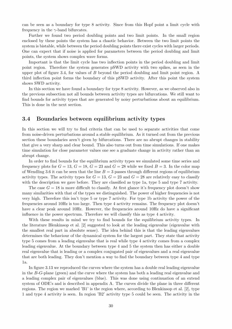
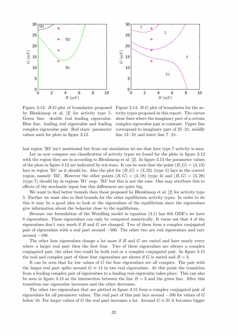
With these results in mind we try to find bounds for the equilibrium activity types. Inthe literature Blenkinsop et al. [2] suggested to look at the leading eigenvalue (eigenvalue withthe smallest real part in absolute sense). The idea behind this is that the leading eigenvaluesdetermines the behaviour of the dynamical system for the largest part. They state that activitytype 5 comes from a leading eigenvalue that is real while type 4 activity comes from a complexleading eigenvalue. At the boundary between type 4 and 5 the system then has either a doublereal eigenvalue that is leading or a complex conjugated pair of eigenvalues and a real eigenvaluethat are both leading. They don’t mention a way to find the boundary between type 4 and type1a.

In figure 3.13 we reproduced the curves where the system has a double real leading eigenvaluein the B-G-plane (green) and the curve where the system has both a leading real eigenvalue anda leading complex pair of eigenvalues (blue). This was done using continuation of an extendsystem of ODE’s and is described in appendix A. The curves divide the plane in three differentregions. The region we marked ’B1’ is the region where, according to Blenkinsop et al. [2], type1 and type 4 activity is seen. In region ’B2’ activity type 5 could be seen. The activity in the

30

0 0.5 1 1.5 2

13.5

14

14.5

15

15.5

16

t (s)

upy(m

V)

G = 13

0 20 400

0.02

0.04

0.06

f (Hz)

pow

er0 0.5 1 1.5 2

11

11.5

12

12.5

13

13.5

t (s)

upy(m

V)

G = 18

0 20 400

0.01

0.02

0.03

0.04

0.05

f (Hz)pow

er

0 0.5 1 1.5 2

9

9.5

10

10.5

11

11.5

t (s)

upy(m

V)

G = 23

0 20 400

0.01

0.02

0.03

0.04

f (Hz)

pow

er

0 0.5 1 1.5 2

8

8.5

9

9.5

10

10.5

t (s)

upy(m

V)

G = 28

0 20 400

0.01

0.02

0.03

0.04

f (Hz)

pow

er

Figure 3.12: From top to bottom simulations for G = 13, G = 18, G = 23 and G = 28, whileB = 3 for all plots. Left: typical time series. Right: frequency plot.

31

0 2 4 6 8 100

5

10

15

20

25

30

B1

B2

B3

B (mV)

G(m

V)

Figure 3.13: B-G-plot of boundaries proposedby Blenkinsop et al. [2] for activity type 5.Green line: double real leading eigenvalue.Blue line: leading real eigenvalue and leadingcomplex eigenvalue pair. Red stars: parametervalues used for plots in figure 3.12.

0 2 4 6 8 100

5

10

15

20

25

30

1b

4

5

7

B (mV)

G(m

V)

Figure 3.14: B-G plot of boundaries for the ac-tivity types proposed in this report. The curvesshow lines where the imaginary part of a certaincomplex eigenvalue pair is constant. Upper linecorrespond to imaginary part of 25 · 2π, middleline 13 · 2π and lower line 7 · 2π.

last region ’B3’ isn’t mentioned but from our simulation we see that here type 7 activity is seen.Let us now compare our classification of activity types we found for the plots in figure 3.12

with the region they are in according to Blenkinsop et al. [2]. In figure 3.13 the parameter valuesof the plots in figure 3.12 are indicated by red stars. It can be seen that the point (B,G) = (3, 13)lays in region ’B1’ as it should be. Also the plot for (B,G) = (3, 23) (type 5) lays in the correctregion, namely ’B2’. However the other points (B,G) = (3, 18) (type 4) and (B,G) = (3, 28)(type 7) should lay in regions ’B1’ resp. ’B3’ but this is not the case. One may attribute this toeffects of the stochastic input but this differences are quite big.

We want to find better bounds then those proposed by Blenkinsop et al. [2] for activity type5. Further we want also to find bounds for the other equilibrium activity types. In order to dothis it may be a good idea to look at the eigenvalues of the equilibrium since the eigenvaluesgive information about the behavior close to the equilibrium.

Because our formulation of the Wendling model in equation (3.1) has 8th ODE’s we have8 eigenvalues. These eigenvalues can only be computed numerically. It turns out that 4 of theeigenvalues don’t vary much if B and G are changed. Two of them form a complex conjugatedpair of eigenvalues with a real part around −500. The other two are real eigenvalues and varyaround −100.

The other four eigenvalues change a lot more if B and G are varied and have nearly everywhere a larger real part then the first four. Two of these eigenvalues are always a complexconjugated pair, the other two could be both real or a complex conjugated pair. In figure 3.15the real and complex part of these four eigenvalues are shown if G is varied and B = 3.

It can be seen that for low values of G the four eigenvalues are all complex. The pair withthe larges real part splits around G ≈ 14 in two real eigenvalues. At this point the transitionfrom a leading complex pair of eigenvalues to a leading real eigenvalue takes place. This can alsobe seen in figure 3.13 as the intersection between the line B = 3 and the green line. After thistransition one eigenvalue increases and the other decreases.

The other two eigenvalues that are plotted in figure 3.15 form a complex conjugated pair ofeigenvalues for all parameter values. The real part of this pair lays around −100 for values of Gbelow 10. For larger values of G the real part increases a lot. Around G ≈ 21 it becomes bigger

32

0 10 20 30−100

−80

−60

−40

−20

0

G (mV)

Re(λ)

0 10 20 300

5

10

15

20

25

30

G (mV)

Im(λ)/(2π)

Figure 3.15: Plots of 4 eigenvalues with larges real part if G is varied and B = 3. Left: realpart. Right: imaginary part divided by 2π.

then smallest real eigenvalue. For G = 30 the real part is close to the largest real eigenvalue.Not shown in the plot is that for larger values of G this pair of complex conjugated eigenvaluesbecomes the leading eigenvalue pair and if G is increased further this pair of eigenvalues becomesunstable and generates a Hopf bifurcation. This Hopf bifurcation is responsible for the birth ofthe limit cycle that generates type 8 activity.

In the right plot of figure 3.15 the complex part of the eigenvalues divided by 2π is plotted.The division by 2π is done because then complex part of the eigenvalues matches with thefrequency that it can generate. One can see that the frequency, of the eigenvalues that form acomplex pair all the time, increases from nearly 0 to nearly 30 if G increases. The frequency ofthe other complex pair stays low as long as it exists.

Let’s try to see how the influence from the eigenvalues is visible in the time series andfrequency plots in figure 3.12. The frequency plots for G = 23 and G = 28 have a peak in thepower spectrum at a frequency that is very close to the imaginary part of the eigenvalue pairthat is complex all the time divided by 2π. The difference can be explained by stochastic effectsof the input that causes the frequency spectrum to be noisy.

For the other two cases displayed in figure 3.12 (forG = 13 andG = 18) this correspondence isless clear. The frequency plot of these cases doesn’t have a clear peak in the frequency spectrum.This can be explained by the fact that the real part of the complex conjugated eigenvalue pair issmall here compared to the real part of the leading eigenvalue. Therefor this eigenvalue has lessinfluence on the system then in the cases G = 23 and G = 28. However it has a small influence.In case G = 18 the frequency spot has a relative large range of frequencies where the power isclose to the maximum power. This can be a consequence of the eigenvalue with large complexpart that would correspond to a frequency of around 12Hz in this case.

With a bit of fantasy the same argument hold for the case G = 13. There the frequencyinduced by this complex conjugated eigenvalue pair is around 5Hz. Another interesting thingin case G = 13 is that also the leading eigenvalue is complex as can be seen in figure 3.15. It’scomplex part is very small and corresponds to a frequency of 0.7Hz. This peak is close to 0 andis difficult to see in the plot.

From our observation we can conclude that the imaginary part of the complex conjugatedeigenvalue pair that always exist has a significant influence on the frequency plots in figure 3.12.The value of the imaginary part divided by 2π gives an indication the main frequency observedin the system. Therefore it is a good idea to use this as criterion for the boundary between the

33

equilibrium activity types.

It’s a good question what frequency forms the bound between two activity types. Activitytype 7 that we distinguished can be seen as a noisy γ-rhythm. Therefore we decide to use thefrequency bounds for the γ-rhythm as a bounds for activity type 7. Wendling et al. [28] usea frequency range between 20-100Hz for the γ-rhythm based on [3]. In an overview article byHughes [16] 25Hz is used as lower bound for the γ-rhythm. In this article it’s also mentioned thatother lower bounds for the γ-rhythm are used, and that it was earlier defined as a rhythm around40Hz. We decided to use 25Hz as lower bound for activity type 7, also because we observed inthe frequency plots that the maximum power goes down a lot if the maximum power lays around25Hz.

Activity type 4 can be seen as an α-rhythm oscillation. In [1] the α-rhythm is said to lay inthe range 7-13Hz, [20] uses 8-13Hz and David and Friston [5] uses 8-12Hz based on [22]. Thesevalues all differ a bit but not much. Based on this we decide to use a frequency range of 7-13Hzfor activity type 4.

This also fixes the ranges for activity type 1b and type 5. Activity type 1b has a lowerfrequency then type 4 so we take this as < 7Hz. Activity type 5 lays between type 4 and type 7and is therefor in the range 13-25Hz.

We continued the boundary curves between the activity types in the B-G-plane using Mat-cont. We therefore used an extended system of ODE’s that continues curves where the imaginarypart of a complex conjugated eigenvalue pair is fixed. A precise description of this method canbe found in appendix A. In figure 3.14 the boundaries we found between the activity types inthe B-G-plane are displayed. In this figure also the parameter values of figure 3.12 are plottedwith a red star. It can be seen that the activity type regions correspond to the activity type weclassified the plot in figure 3.12.

3.5 Activity map for the B-G-plane

In section 3.3 we did bifurcation analysis in B for fixed values of G. In this way different codim1 bifurcations were found: Hopf, limit point and homoclinic bifurcations. We saw that thesebifurcations form the boundary between some of the activity types. Further we also foundout that a limit cycle could have an inflection point that gives a false bifurcation. This falsebifurcation is the boundary between type 6 and type 3 activity. In the previous section wediscussed how we could find suitable borders between the other activity types, which all camefrom noisy perturbations around a stable equilibrium, and presented a way to continue them intwo parameters. In this section we will put these results together.

Using Matcont we continue the codim 1 bifurcations, which we found with the bifurcationanalysis in B, in B and G. We also want to continue inflection points in two parameters. Since aninflection point is not a bifurcation, there is no direct method implemented in Matcont to do this.In [23] a method for continuation of inflection points of limit cycles is proposed using a periodicboundary value problem. They provide a link to an implementation for DDE-BIFTOOl (anotherpackage for numerical bifurcation analysis), but unfortunately this isn’t available anymore.

To find a reasonable approximation of the inflection point curve in B and G we use thefollowing method. We continue from a large number of points at the Hopf bifurcation curve,a limit cycle in B. For each of these limit cycle curves we detect the value at which the limitcycle gets an extra maximum. In this way we obtain values of B and G that approximate theinflection point curve.

The continuation of the codim 1 bifurcations, the inflection points and the boundaries for theequilibrium activity types are displayed in figure 3.16. Here a map for the different activity typesfor (B,G) ∈ [0, 50]× [0, 50] is shown. The numbers in this figure correspond to the numbers ofthe activity types.

In the figure we see the following things. Type 7 and type 8 activity are seen for high values

34

0 5 10 15 20 25 30 35 40 45 500

10

20

30

40

50

CPC

NCH

B (mV)

G(m

V)

1a

1b

2 234

5

6

7

8

Figure 3.16: Plot of activity types found in B-G-plane. The solid blue line represent a curve oflimit points. The dashed blue lines also represent curves of limit points but then for I = 90±3σ.The green line (almost on the blue line) is the curve of homoclinic bifurcations. Red lines indicateHopf bifurcations. The black line is a period doubling curve. The cyan line indicate a limit pointof cycle curve. The other colors indicate lines that are not bifurcations. The orange line indicatesthe curve of inflection points in the limit cycle. The magenta lines indicate a constant imaginarypart of an eigenvalue.

of G and low values of B. For these values the slow inhibitory cells don’t play a big role. Themain inhibition of the system is done by the fast inhibitory cells. This causes the high frequenciesseen for type 7 and 8. Type 7 activity has, besides with type 8, a boundary with type 5 activity.Type 5 activity borders to type 4 activity. For this type of activity the main inhibition comesfrom the slow inhibitory cells, this causes the noisy α-rhythm seen for this type of activity.

From type 4 activity we can go to type 1b activity. This is seen for low values of B and G.In this case there is nearly no inhibition. Therefore the potential of the pyramidal cells, upy,is high for this case. Besides type 1b and type 5 activity type 4 has also a border with type 6activity. This is the curve of Hopf bifurcations. Type 6 activity can be seen for mid values of Bat all values of G. This is the result of the slow inhibition of the fast inhibitory cells. For midvalues of B the fast inhibitory cells are inhibited so much by the slow inhibitory cells that alsofor high values of G they doesn’t have much influence on the pyramidal cells.

As mentioned before we can pas from type 6 activity to type 3 activity if we cross theinflection point curve. If B is increased further we see first sporadic SWDs (type 2) and latertype 1a activity. In the region with type 1a activity the inhibition is large compared to theexcitation and the potential of the pyramidal cells is low.

For mid values of B and high values of G we see in figure 3.16 some other activity regions.The black curve represents a curve of period doublings. Inside this curve there lays a perioddoubling curve of the period doubled cycle (not shown in figure 3.16) and the system generateschaotic activity. A bit to the right a second curve of inflection points is shown. In this regionthe system has a stable limit cycle with two spikes followed by a wave, like we saw in the upperplot of figure 3.4.

Our activity map in figure 3.16 agrees for a large part with the colour map of Wendling etal. [28] (see figure 3.6). The main difference is that type 6 activity in our figure is seen for allvalues of G if B is at an intermediate value. In the map by Wendling this is only for lower valuesof G, for higher values of G they call this type 4 activity. We pointed at this difference before,it’s probably a difference in the definition of the activity types.

35

In this section we showed an activity map for (B,G) ∈ [0, 50]× [0, 50]. Some of the bound-aries between the different activity types were formed by continuation of codim 1 points in twoparameters. In order to understand how these codim 1 points are connected and from whatcodim 2 points they arise we will look in the next section at the continuation of these bifurcationfor a broader parameter range.

3.6 Continuation of codim 1 bifurcations

In this section a codim 1 bifurcation diagram is presented for a much bigger region of parametersB andG. This can be found in figure 3.17. A large part of this region will correspond to physicallyunrealistic values, because B or G is negative or extremely large. However, some codim 2 pointsare found for these values. Some of these codim 2 points are starting points of codim 1 curves,like Bodagnov-Takens or zero-Hopf (fold-Hopf) points.

In figure 3.17 one can see that the two limit point curves of figure 3.16 are connected to eachother via several cusp points and form a closed curve in the B-G-space. In the upper inset offigure 3.16 one can see that around (B,G) = (15, 400) this curve crosses itself and there are twocusp points close to this point. In this way, a small region with a triangular shape is formed.In this region the system has five equilibria. Inside the rest of the region enclosed by the curvethere are 3 equilibria.

Along the big limit point curve two zero-Hopf points are detected. At a zero-Hopf point acurve of Hopf bifurcations intersects tangential to the curve of limit points. The normal formcoefficients provided by Matcont are (s, θ) ≈ (−1,−0.96) for the zero-Hopf point around B = 0and (s, θ) ≈ (1, 1.96) for the zero-Hopf point around B = 20. Because for both points thecoefficients s and θ have the same sign the zero-Hopf point has a relatively simple normal form:there don’t start Neymarck-Sacker and homoclinic curves from this point [13].

It turns out that the two zero-Hopf points are connected by a closed curve of Hopf points.This curve of Hopf points is the one that generates the limit cycle with high frequency found inthe bifurcation diagram for B in case G = 50. Along this curve of Hopf points two generalizedHopf (GH) points are found. At a generalized Hopf point the Hopf bifurcation turns fromsubcritical to supercritical and v.v. It’s also the starting point for a limit point of cycle (LPC)curve. One can see that the two GH points on the fast Hopf curve are connected via a LPCcurve.

The Hopf points, found in the bifurcation diagrams for B as the point from which theapproximately 10Hz limit cycle starts, are part of a curve of Hopf points that start at theBodagnov-Takens point at (B,G) ≈ (55, 1535). From this Bodagnov-Takens point also startsthe curve of homoclinic bifurcations that causes the SWD cycle to disappear. The homocliniccurve sometimes falls together with a limit point forming a saddle-node on an invariant curve(SNIC). This homoclinic curve ends at the Bodagnov-Takens point around B ≈ 47 and G ≈ −97.The Hopf curve that starts from this Bodagnov-Takens point continues for values of G far belowzero.

The Hopf curve that starts from the Bodagnov-Takens point at (B,G) ≈ (55, 1535) also has ageneralized Hopf bifurcation at (B,G) ≈ (54, 1450). From this point starts a limit point of cyclecurve. On this curve lay both limit point of cycles that are detected during the continuation inB for G = 50. Also the cusp point of cycles seen in figure 3.16 lays on this curve. This curve hasanother cusp point of cycles around (B,G) ≈ (41, 558). From there on the limit point of cyclecurve walks close along the homoclinic bifurcation curve till it stops at the point marked ’NH’that lays on the homoclinic curve. The point ’NH’ indicates a neutral homoclinic orbit, i.e. apoint where the saddle quantity of the homoclinic orbit is zero [15].

Further we see from figure 3.17 that the two period doubling points found for continuationin B for G = 50 are connected with each other with a closed curve. Along this curve there wereno codim 2 bifurcations detected. Inside the region enclosed by the period doubling curve there

36

lays a period doubling curve of the period doubled limit cycle, for clarity this curve is not shownin figure 3.17. In the region enclosed by the period doubling curve the system is chaotic and thesystem produces limit cycles with a complex wave shape.

37

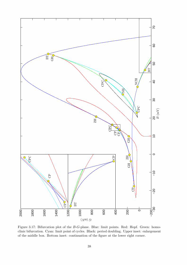
−30

−20

−10

010

2030

4050

6070

−20

00

200

400

600

800

1000

1200

1400

1600

1800

2000

NCH

B(m

V)

G(mV)

CP

ZH

CP

CP

ZH

BT

BT

GH

GH

GH

CPC

CPC

CPC

NH

BT

CP

BT

GH

CP

CP

CPC

Figure 3.17: Bifurcation plot of the B-G-plane. Blue: limit points. Red: Hopf. Green: homo-clinic bifurcation. Cyan: limit point of cycles. Black: period doubling. Upper inset: enlargementof the middle box. Bottom inset: continuation of the figure at the lower right corner.

38

Chapter 4

Conclusion & discussion

In this report we gave an overview of neural mass models for cortical columns. After this weinvestigated the neural mass model by Wendling et al. [28] in more detail. A feature of theWendling model is that it has two inhibitory populations. These two populations both giveinhibitory feedback to the pyramidal cells but with a different timescale. Our main target wasto find out what types of activity this model can generate and what the influence of inhibitionon these activity types is.

We gave a description of different activity types that can be seen in the Wendling model.A part of these activity types was also described by Wendling et al. [28] and by Blenkinsop etal. [2]. We distinguished two new activity types. One is a γ-oscillation that is generated by alimit cycle. The other is noisy γ-activity that arises from noise-driven perturbations around anequilibrium.

Our description of the activity types was done in a more mathematical way then that ofWendling et al. [28]. In the description of the activity types we looked at the origin of theactivity, i.e does the activity come from a limit cycle or from noisy perturbations around anequilibrium point.

After this we did bifurcation analysis and investigated the influence of the synaptic gain ofthe slow inhibitory PSP (B). It turned out that the bifurcations we found explain the transitionbetween activities that are generated from a limit cycle and those that are generated from noisyperturbations around an equilibrium. The boundary between α-oscillations and noisy α-activitywas formed by a Hopf bifurcation. This bifurcation gives a strict bound between these activities.

The bound between SWD and normal background activity was found to be a limit pointbifurcation if no noise was added to the system. If the system receives a noisy input then thereexist a transition region where sporadic SWD’s were seen. As bounds for this transition regionwe proposed to use the limit point curves for a fixed input of µ ± 3σ, where µ is the mean ofthe input and σ is the standard deviation. This because the location of this limit point is verysensible for a change in input.

Our explanation for the sporadic spike activity is different from that given by Blenkinsop etal. [2]. They suggest that the sporadic spikes are a consequence of the fact that the period of alimit cycle goes to infinity if the limit cycle approaches a homoclinic bifurcation. Limit cyclesclose to a homoclinic bifurcation are for a relatively long time close to the equilibrium point ofthe homoclinic curve and are a relatively short time far away from it. Our explanation seemsmore logical, because it also explains the effect of the input noise strength which is related tothe size of the sporadic spike region.

To find the other transitions between activity types we needed other criteria. Blenkinsop etal. found out that the transition between α-rhythm oscillations and SWD was a consequenceof an inflection point in the limit cycle. This inflection point gives a strict boundary betweenthese two activities. If this boundary is crossed one sees an immediate change in the dynamicsof the system. It happens also in other models for neuronal activity that the transition between

39

α-oscillations and SWD is formed by an inflection point, for example in the thalamo-corticalmodel discussed by Breakspear et al. [4].

In [23] a method is proposed to continue these inflection points in two parameters. Unfor-tunately, we couldn’t found an implementation of this method. Therefore we applied a workaround to continue a curve of inflection points. A future task may be to make an implementationof this method in order to continue curves of inflection points in an easy way.

Further we wanted to find the transitions between activity types that are generated fromnoisy perturbations around an equilibrium. We found a reasonable bound for these activitiesby looking at the imaginary part of a complex conjugated pair of eigenvalues of the equilibriumpoint. The imaginary part of this eigenvalue divided by 2π gave approximately the frequencythat had the highest power. We presented a way to continue curves with a constant imaginarypart of this eigenvalue and used this to separate the equilibrium activity types.

The boundaries we choose for these equilibrium activity types correspond to a peak of 7,13 and 25Hz in the frequency spectrum. These values were chosen by using the bounds of thefrequency bands for α- and γ-activity found in literature. About the precise value of thesebounds can be discussed. The bounds for the α- and γ-band in literature vary also. However, itturns out that the precise value doesn’t matter because the bounds between these activity typesare soft. One doesn’t see an immediate change in activity but more a gradual change. Thereforeone must see these borders more as a rough indication.

In the activity map we found for the synaptic gains of the two inhibitory PSPs we saw thatslow inhibition has more influence then fast inhibition. The activity types that arises due to theslow inhibition (activity types with a frequency in the α range) are seen in large regions of theparameter space, including relatively high values of the fast synaptic gain. In contrast to theactivity types that arise from purely the fast inhibitory PSP (activity types with a frequency inthe γ range). These are seen only for high values of fast synaptic gain and low values of the slowsynaptic gain. The reason for this is that the slow inhibitory cells project to the fast inhibitorycells and therefore inhibit the influence of the fast inhibitory PSP.

In the regions were both the fast and the slow inhibitory PSP play a role the system producesan activity type with a frequency in the range 13-25Hz. This activity has a relatively lowamplitude. It can be compared with the fast onset activity seen at a seizure onset [28]. In themodel this activity is a mixture of the two timescales. It’s in fact the same phenomenon asdescribed by David & Friston [5]. This activity type arises from noisy perturbations around anequilibrium. There is no equivalent activity type that is generated from a stable limit cycle withthe same frequency. This in contrast to the α- and γ-activity that arises both as limit cycleactivity and as equilibrium activity.

Another effect of the fast inhibitory process can be seen at high values of the fast synapticgain and medium values of the slow one. In this region the model is able to produces pSWDwith two or three spikes and other complex activities. These type of activities are also observedin the model by Goodfellow et al. [10] that also has two different inhibitory timescales, but notin the Jansen & Rit model that has only the slow one. According to [2] these activity types arecommonly observed in EEGs of epilepsy patients.

We can conclude that although the fast inhibition doesn’t have a large influence on theactivity types it does play an important role. It is crucial in the generation of some epileptogenicactivity types like fast onset activity and pSWD. Realistic NMMs that try to model typesof epilepsy that features these activities, should therefore include a fast and slow inhibitorytimescale.

In this report we investigated the activity of one single neural mass. However, in mostneural mass models multiple cortical columns are coupled together. It is interesting to see ifthis produces other, more complex, types of activity and how this affects the activity map.Especially in cases were the cortical columns don’t have the same parameters. In this way onehas a heterogeneous network of cortical columns that comes closer to the reality.

40

Appendix A

Continuation of non-bifurcations

In this chapter is described how certain non-bifurcation points can be continued using bifurcationsoftware like Matcont. Therefore we extend the system we investigate with some extra differentialequations. First is described how eigenvalues of an equilibrium point can continued. Then amethod is described that has a limit point if a linear combination of system variables has acertain value. We will combine these two principles to give extended systems that are able tocontinue the curves discussed in chapter 3.4.

In the whole chapter we will use that x = f(x, α) denote the original system of differentialequations, where x ∈ Rn represent the system variables and α ∈ Rm the parameters. Furtherwe define J to be the Jacobian of the original system:

J(x, α) :=∂f(x, α)

∂x.

A.1 Continuation of eigenvalues

In this section we describe how a system of differential equations can extended in a way that theeigenvalues can continued as system variables. First we will treat this for a real eigenvalue andlater for a complex conjugated pair of eigenvalues.

A.1.1 Continuation of a real eigenvalue

Let λ ∈ R be an eigenvalue of J and v a corresponding eigenvector. Then by definition it holdsthat:

Jv = λv ⇐⇒ Jv − λv = 0. (A.1)

We can require v to have unit length:

< v, v >= 1 ⇐⇒ < v, v > −1 = 0, (A.2)

where < ·, · > denotes the standard innerproduct on Rn.

We extend the original system of differential equations in the following way:

x = f(x, α), (A.3a)

v = Jv − λv, (A.3b)

λ =< v, v > −1. (A.3c)

From the results in equations (A.1) and (A.2) it’s clear that this system has an equilibrium pointif x is an equilibrium point of the original system and v is an eigenvector with unit length to theeigenvalue λ of the linearization of this equilibrium.

41

We can continue an equilibrium of the extended system (A.3) in one parameter. However, itcould be that the extra equations cause that the extended system gets additional limit points.It turns out that this is the case only if the multiplicity of the eigenvalue is greater then 1.

To prove this we compute the Jacobian of the extended system: J 0 0∂(Jv)∂x J − λI −v0 2vT 0

.This matrix is a block lower triangular matrix. We know that the extended system has a limitpoint if it’s Jacobian has an eigenvalue 0. This is the case if J has a zero eigenvalue or thematrix

K :=

[J − λI −v

2vT 0

],

has a zero eigenvalue. The matrix J has a zero eigenvalue if the original system has a limitpoint.

We know that the matrix K has an eigenvalue 0 if we can find a vector y ∈ Rn and a scalarα ∈ R such that (y, α) 6= 0 and:[

00

]= K

[yα

]=

[J − λI −v

2vT 0

] [yα

]=

[(J − λI)y − αv

2vT y

](A.4)

If we multiply the upper block with (J − λI) from the left it follows that:

0 = (J − λI)2y − α(J − λI)v = (J − λI)2y,

since (J − λI)v = 0 because v is an eigenvector of J . So we find that

y ∈ N (J − λI)2 ,

where N (J − λI)2 denotes the nullspace of (J − λI)2.In case λ is a simple eigenvalue of J (λ is an eigenvalue with algebraic multiplicity one),

it follows from generalized eigenvalue theory that N (J − λI) = N (J − λI)2. Since v is aneigenvalue of J we know that v 6= 0 and v ∈ N (J − λI). From the assumption that λ is a simpleeigenvalue it follows that dim (N (J − λI)) = 1. So v spans N (J − λI). Therefore y = γv forsome γ ∈ R. From the bottom entries in equation (A.4) it follows that:

0 = 2vT y = 2γvT v = 2γ =⇒ γ = 0 =⇒ y = 0,

where we used that vT v =< v, v >= 1. So y = 0. From the upper entries in equation (A.4) wefind:

0 = (J − λI)y − αv = −αv.Since v 6= 0, it’s an eigenvector, we must have α = 0. It follows that the (y, α) = 0 and thereforethe matrix K doesn’t have an eigenvalue 0. This means that as long as the matrix J has asimple eigenvalue the extended system don’t have additional limit points.

In case λ is not a simple eigenvalue of J then we can distinct two sub cases. In the first subcase dim (N (J − λI)) ≥ 2. Then we can find a y such that < y, v >= 0 and y an eigenvector ofJ . It’s easy to see that (y, 0) in this case is a non trivial solution of (A.4). So K has a eigenvalue0.

In the second sub case the matrix doesn’t have a full eigenspace. We have

dim (N (J − λI)) = 1.

In this case it’s known that there exist a y such that < v, y >= 0 and (J − λI)y = v. In thiscase (y, 1) is a non-trivial solution of (A.4). It follows that 0 is an eigenvalue of K in this case.

So we showed that the extended system (A.3) can continue a real eigenvalue of the originalsystem. The extended system (A.3) has limit points if the original system has a limit point orif the eigenvalue that is continued is non-simple. The latter is generally the case if two realeigenvalues fall together and form a pair of complex conjugated eigenvalues.

42

A.1.2 Continuation of a complex conjugated pair of eigenvalues

Now we focus on continuing a complex conjugated pair of eigenvalues. Let µ+ iθ be a complexeigenvalue of J where µ ∈ R and θ ∈ R≥0. Denote the corresponding eigenvector by p+ iq withp, q ∈ Rn. Then by definition it holds that:

J(p+ iq) = (µ+ iθ)(p+ iq) = (µp− θq) + i(θp+ µq).

Splitting the real and imaginary part gives:

0 = Jp− µp+ θq, (A.5a)

0 = Jq − θp− µq. (A.5b)

Like in the real case we can require that the eigenvector p+ iq has unit length. In terms ofthe innerproduct on Rn this gives.

0 =< p, p > + < q, q > −1, (A.6)

In the complex case we have an addition degree of freedom. Therefore we can require that:

0 =< p, q > . (A.7)

In the complex case we extend the original system of differential equations to the followingsystem of 3n+ 2 equations:

x = f(x, α), (A.8a)

p = Jp− µp+ θq, (A.8b)

q = Jq − θp− µq, (A.8c)

µ =< p, p > + < q, q > −1, (A.8d)

θ =< p, q > . (A.8e)

From the results in equations (A.5), (A.6) and (A.7) it’s clear that this system has anequilibrium point if x is an equilibrium point of the original system and p+ iq is an eigenvectorto the eigenvalue µ+ iθ of the linearization of this equilibrium.

A.2 Limit point at certain value of system variables

In this section is explained how a curve can continued at which a linear combination of thesystem variable has a certain value. So we want to find a curve in a two parameter space where< w, x >= c for some vector w ∈ Rn and c ∈ R. In order to do this we extend the system withan auxiliary variable h ∈ R in the following way:

x = f(x, α), (A.9a)

h =< w, x > −h2 − c. (A.9b)

It can seen that this extended system has an equilibrium if x is an equilibrium of the originalsystem and h = ±√< w, x > −c. It follows that h is real in case < w, x > −c ≥ 0. Sothis extended system doesn’t have a real equilibrium everywhere the original system has anequilibrium.

43

Further the extended system in (A.9) has a limit point at < w, x >= c. To prove this wecompute the Jacobian of this extended system. This gives:

[J 0wT 2h

].

We see that the Jacobian of the extended system is again lower triangular. Therefore theeigenvalues are given by those of J and the scalar 2h. The first one causes that the extendedsystem has a limit point if the original system has a limit point. The scalar 2h gives a limitpoint if h = 0. Since we know that h at an equilibrium point is given by h = ±√< w, x > −c itfollows that h = 0 if and only if < w, x >= c. So the auxiliary variable h gives a limit point ifand only if < w, x >= c.

The extended system in equation (A.9) can be used to start an equilibrium continuation froma point in a two parameter space where < w, x >≥ c. This equilibrium can continued until alimit point induced by the auxiliary variable h is reached. This is easy to see since h = 0 inthis case. The obtained limit point can continued in two parameters and gives a curve where< w, x >= c.

A.3 Continuation of possible boundaries of activity types

In the previous two sections different extensions of a system of differential equations are discussed.In this section is showed how these extensions can be used in order to continue the boundariesof activity types as discussed in chapter 3.4. We start with the boundaries used by Blenkinsopet al. [2]. After this the extended system, that is used to continue the boundaries where theimaginary part of a complex eigenvalue is fixed, is given.

A.3.1 Transition of leading eigenvalue

To distinguish the different activity types in the Wendling model Blenkinshop et al. [2] proposedto use the curve that is the transition between a real and complex leading eigenvalue as boundary.This transition can take place in two ways. Case 1: the system has two real eigenvalue thatcollide and form a complex pair. In this case the system has a double real eigenvalue at theboundary. Case 2: the system has a real eigenvalue, say λ, and a complex conjugated eigenvaluepair, say µ+ iθ. Due variation of the parameters µ can get bigger then λ. At the boundary wehave in this case λ = µ.

To find these boundaries by numerical continuation we use the methods described in thesections before. To find the place where the system has a double leading real eigenvalue we needto continue the real eigenvalue that is leading. This can we do by extending the original systemsas described in equation (A.3) and continue the leading real eigenvalue. From section A.1.1 weknow that this system has a limit point in case the system has a double reel eigenvalue. Onecan continue this limit point in two variable two obtain a curve where the system has a doubleleading eigenvalue.

For case 2 we need to continue also a complex conjugated pair of eigenvalues. Thereforewe extend our system with both equations from (A.3) and (A.8). We want that the systemhas a limit point if the real eigenvalue is as big as the real part of the complex eigenvalue, soλ−µ = 0. To do this we extend this extended system with the method described in section A.2.

44

All together we get the following big system:

x = f(x, α), (A.10a)

v = Jv − λv, (A.10b)

λ =< v, v > −1, (A.10c)

p = Jp− µp+ θq, (A.10d)

q = Jq − θp− µq, (A.10e)

µ =< p, p > + < q, q > −1, (A.10f)

θ =< p, q >, (A.10g)

h = (λ− µ)− h2. (A.10h)

This big system has an equilibrium in the region where λ ≥ µ and has limit points in case thesystem has a double real eigenvalue and in case the real part of the complex eigenvalue becomeslarger then the real eigenvalue.

This system must be initialized at an equilibrium point of the original system. The leadingreal eigenvalue, it’s corresponding eigenvector and the complex eigenvalue of which the real partbecomes larger then the leading real eigenvalue and it’s eigenvector must also be filled in asinitial conditions.

A.3.2 Continuation of eigenvalues with a fixed imaginary part

For the boundaries between equilibrium activity types we wanted to find curves where theimaginary part of a complex eigenvalue is fixed at some value. In order to do this we extend thesystem as described in section A.1.2 to continue a complex eigenvalue. This extended system weextend again by the method described in section A.2. We obtained the following system:

x = f(x, α), (A.11a)

p = Jp− µp+ θq, (A.11b)

q = Jq − θp− µq, (A.11c)

µ =< p, p > + < q, q > −1, (A.11d)

θ =< p, q >, (A.11e)

h = −θ − h2 + c. (A.11f)

This extended system has a limit point in case the imaginary part of the eigenvalue θ equalsthe desired imaginary part c. It must be initialized in a region where c ≥ θ and then continuedin one parameter till a limit point induced by the auxiliary variable h is reached. The obtainedlimit point can be continued in two parameters to obtain a curve in the parameter space.

45

Appendix B

Simulation source code

In this appendix our implementation for the Wendling model is given. This implementation iswritten in Matlab and uses the Milstein method to solve the stochastic differential equations inequation (3.1) numerically. The source code contains some comments that explain the differentvariables and the algorithm.

1 t ic ; %To measure computation time2 %% Simulat ion s e t t i n g s3 Npart=2; %Number o f pa r t s f o r f o u r i e r transform inc l u d i n g i n t i a l

par t4 Tend=10∗Npart ; %Total s imu la t i on time5 NTST=Tend∗10000; %Number o f Time Steps6 Nout=5; %Output every 5 th t imes t ep78 d e l t a t=Tend/NTST; %Timestep s i z e9

10 %% Parameter s e t t i n g s11 A=5; %Average e x c i t o r y synap t i c gain12 B=25; %Average s low i n h i b i t o r y synap t i c gain13 G=15; %Average f a s t i n h i b i t o r y synap t i c gain1415 a=100; %Inver se o f e x c i t o r y time cons tant16 b=50; %Inver se o f s low i n h i b i t o r y time cons tant17 g=500; %Inver se o f f a s t i n h i b i t o r y time cons tant1819 C=135; %Connec t i v i t y parameter20 C1=C;21 C2=0.8∗C;22 C3=0.25∗C;23 C4=0.25∗C;24 C5=0.3∗C;25 C6=0.1∗C;26 C7=0.8∗C;2728 pf =90; %Mean input29 sd=2; %Standard d e v i a t i on input3031 %% I n i t i a l c ond i t i t o n s32 x=zeros ( 4 , 1 ) ;33 y=zeros ( 4 , 1 ) ;3435 %% I n i t i a l i s e v a r i a b l e s f o r computation36 Im=eye ( 4 , 4 ) ;3738 Q1=−de l t a t ∗diag ( [ a ˆ2 , a ˆ2 ,bˆ2 , g ˆ 2 ] ) ;39 Q2=Im−2∗de l t a t ∗diag ( [ a , a , b , g ] ) ;40 Q3=de l t a t ∗diag ( [A∗a ,A∗a ,B∗b ,G∗g ] ) ;41

46

42 fd =[0;A∗a∗pf /C2 ; 0 ; 0 ] ∗ de l t a t ;43 f s =[0 ;A∗a/C2 ; 0 ; 0 ] ∗ sqrt ( d e l t a t ) ∗ sd∗randn (1 ,NTST) ;4445 P=[ [0 , C2 , −C4,−C7 ] ;46 [C1 , 0 , 0 , 0 ] ;47 [C3 , 0 , 0 , 0 ] ;48 [C5,0 ,−C6 , 0 ] ] ;4950 u=P∗x ;51 uout=zeros (4 , ce i l (NTST/Nout )+1) ;52 uout ( : , 1 )=u ;5354 xn=zeros ( 4 , 1 ) ;55 yn=zeros ( 4 , 1 ) ;5657 %%58 t1=toc ;59 disp ( [ ’ I n i t i a l i s a t i o n time : ’ ,num2str( t1 ) ] ) ;60 disp ( ’ S ta r t s imu la t i on ’ ) ;6162 t e l =0;63 indexp lo t =2;64 for i =1:NTST65 xn=x+de l t a t ∗y ;66 yn=Q1∗x+Q2∗y+Q3∗ sigm (u)+fd+f s ( : , i ) ;6768 x=xn ;69 y=yn ;70 u=P∗x ;7172 %Saves u f o r output every Nout i t e r a t i o n s73 t e l=t e l +1;74 i f t e l==Nout75 t e l =0;76 uout ( : , i ndexp lo t )=u ;77 indexp lo t=indexp lo t +1;78 end79 end8081 t2=toc ;82 disp ( [ ’ S imulat ion complete , durat ion : ’ ,num2str( t2−t1 ) ] ) ;8384 %% Post p roce s s ing8586 %Plot time s e r i e s87 f igure ;88 plot ( 0 : d e l t a t ∗Nout : Tend , uout ( 1 , : ) ) ;89 xlim ( [ 0 Tend ] )90 set (gca , ’YDir ’ , ’ r e v e r s e ’ ) ;9192 %Ca l cu l a t e f requency spectrum93 for j =1:Npart−1;94 [ f , pow]= f r e q p l o t ( uout (1 , f loor (NTST∗ j /( Npart∗Nout ) ) : f loor (NTST∗( j +1)/(Npart∗

Nout ) ) )−mean( uout (1 , f loor (NTST∗ j /( Npart∗Nout ) ) : f loor (NTST∗( j +1)/(Npart∗Nout ) ) ) ) ,1/( d e l t a t ∗Nout ) ) ;

95 i f j >1;96 powtot=powtot+pow ;97 else98 powtot=pow ;99 end

100 end101102 %Disp lay f requency spectrum

47

103 f igure ;104 plot ( f , powtot /(Npart−1) ) ;105 xlim ( [ 0 5 0 ] )106107 toc ; %Disp lays t o t a l computation time

48

Bibliography

[1] B. S. Bhattacharya, D. Coyle, and L. P. Maguire. A thalamo-cortico-thalamic neural massmodel to study alpha rhythms in alzheimer’s disease. Neural Networks, 24(6):631–645, 2011.

[2] A. Blenkinsop, A. Valentin, M. P. Richardson, and J. R. Terry. The dynamic evolution offocal-onset epilepsies - combining theoretical and clinical observations. European Journalof Neuroscience, 36(2):2188–2200, 2012.

[3] A. Bragin, J. Engel Jr., C. L. Wilson, I. Fried, and G. W. Mathern. Hippocampal andentorhinal cortex high-frequency oscillations (100-500 hz) in human epileptic brain and inkainic acid-treated rats with chronic seizures. Epilepsia, 40(2):127–137, 1999.

[4] M. Breakspear, J. A. Roberts, J. R. Terry, S. Rodrigues, N. Mahant, and P. A. Robinson.A unifying explanation of primary generalized seizures through nonlinear brain modelingand bifurcation analysis. Cerebral Cortex, 16(9):1296–1313, 2006.

[5] O. David and K. J. Friston. A neural mass model for meg/eeg: Coupling and neuronaldynamics. NeuroImage, 20(3):1743–1755, 2003.

[6] O. David, L. Harrison, and K. J. Friston. Modelling event-related responses in the brain.NeuroImage, 25(3):756–770, 2005.

[7] G. Deco, V. K. Jirsa, P. A. Robinson, M. Breakspear, and K. Friston. The dynamic brain:From spiking neurons to neural masses and cortical fields. PLoS Computational Biology,4(8), 2008.

[8] A. Dhooge, W. Govaerts, and Yu A. Kuznetsov. Matcont: A matlab package for numericalbifurcation analysis of odes. ACM Transactions on Mathematical Software, 29(2):141–164,2003.

[9] WJ Freeman. Models of the dynamics of neural populations. Electroencephalography andclinical neurophysiology. Supplement, (34):9–18, 1977.

[10] M. Goodfellow, K. Schindler, and G. Baier. Intermittent spike-wave dynamics in a hetero-geneous, spatially extended neural mass model. NeuroImage, 55(3):920–932, 2011.

[11] M. Goodfellow, K. Schindler, and G. Baier. Self-organised transients in a neural mass modelof epileptogenic tissue dynamics. NeuroImage, 59(3):2644–2660, 2012.

[12] F. Grimbert and O. Faugeras. Bifurcation analysis of jansen’s neural mass model. Neuralcomputation, 18(12):3052–3068, 2006.

[13] J. Guckenheimer and Y. A. Kuznetsov. Fold-Hopf bifurcation. Scholarpedia, 2(10):1855,2007. revision 91277.

[14] R. Hindriks and M. J. A. M. van Putten. Meanfield modeling of propofol-induced changesin spontaneous eeg rhythms. NeuroImage, 60(4):2323–2334, 2012.

49

[15] A. J. Homburg and B. Sandstede. Homoclinic and heteroclinic bifurcations in vector fields,volume 3 of Handbook of Dynamical Systems. 2010.

[16] J. R. Hughes. Gamma, fast, and ultrafast waves of the brain: Their relationships withepilepsy and behavior. Epilepsy and Behavior, 13(1), 2008.

[17] B. H. Jansen and V. G. Rit. Electroencephalogram and visual evoked potential generationin a mathematical model of coupled cortical columns. Biological cybernetics, 73(4):357–366,1995.

[18] B. H. Jansen, G. Zouridakis, and M. E. Brandt. A neurophysiologically-based mathematicalmodel of flash visual evoked potentials. Biological cybernetics, 68(3):275–283, 1993.

[19] Y.A. Kuznetsov. Elements of Applied Bifurcation Theory. Springer, 3th edition, 2004.

[20] F. H. Lopes da Silva, A. Hoeks, H. Smits, and L. H. Zetterberg. Model of brain rhythmicactivity. the alpha rhythm of the thalamus. Kybernetik, 15(1):27–37, 1974.

[21] F. H. Lopes da Silva, A. van Rotterdam, P. Barts, E. van Heusden, and W. Burr. Modelsof Neuronal Populations: The Basic Mechanisms of Rhythmicity, volume 45 of Progress inBrain Research. 1976.

[22] PL Nunez. Electric fields of the brain, 1981. Oxford University Press, New York, 1981.

[23] S. Rodrigues, D. Barton, F. Marten, M. Kibuuka, G. Alarcon, M. P. Richardson, and J. R.Terry. A method for detecting false bifurcations in dynamical systems: Application toneural-field models. Biological cybernetics, 102(2):145–154, 2010.

[24] R. C. Sotero, N. J. Trujillo-Barreto, Y. Iturria-Medina, F. Carbonell, and J. C. Jimenez.Realistically coupled neural mass models can generate EEG rhythms. Neural computation,19(2):478–512, 2007.

[25] Cornelis J Stam. Nonlinear brain dynamics. Nova Publishers, 2006.

[26] J. Touboul, F. Wendling, P. Chauvel, and O. Faugeras. Neural mass activity, bifurcations,and epilepsy. Neural computation, 23(12):3232–3286, 2011.

[27] A. van Rotterdam, F. H. Lopes da Silva, J. van den Ende, M. A. Viergever, and A. J.Hermans. A model of the spatial-temporal characteristics of the alpha rhythm. Bulletin ofmathematical biology, 44(2):283–305, 1982.

[28] F. Wendling, F. Bartolomei, J. J. Bellanger, and P. Chauvel. Epileptic fast activity canbe explained by a model of impaired gabaergic dendritic inhibition. European Journal ofNeuroscience, 15(9):1499–1508, 2002.

[29] F. Wendling, F. Bartolomei, F. Mina, C. Huneau, and P. Benquet. Interictal spikes, fastripples and seizures in partial epilepsies - combining multi-level computational models withexperimental data. European Journal of Neuroscience, 36(2):2164–2177, 2012.

[30] F. Wendling, J. J. Bellanger, F. Bartolomei, and P. Chauvel. Relevance of nonlinear lumped-parameter models in the analysis of depth-eeg epileptic signals. Biological cybernetics,83(4):367–378, 2000.

[31] F. Wendling, A. Hernandez, J. . Bellanger, P. Chauvel, and F. Bartolomei. Interictal toictal transition in human temporal lobe epilepsy: Insights from a computational model ofintracerebral EEG. Journal of Clinical Neurophysiology, 22(5):343–356, 2005.

50