Embed Size (px)
Citation preview
Hybrid adaptive observer for
controlling a Brushless DC Motor(MASTER THESIS BY GROUP 1032C)
AALBORG UNIVERSITY · AAUDepartment of Electronic Systems
Master Thesis, May 2007
Group 1032c

This page is left intentionally blank
Intelligent Autonomous Systems
Fredrik Bajers Vej 7C
9220 Aalborg Ø, Denmark
Telephone +45 96 35 87 00
Fax +45 98 15 17 39
Title:
Hybrid adaptive observer for con-
trolling a Brushless DC Motor
Semester:
10th, IAS
Project group:
1032c
Supervisors:
Jan Dimon Bendtsen
Carsten Skovmose Kallesøe
Group Members:
Piotr Niemczyk
Thomas Porchez
Copies: 7
Report pages: 98
Appendices pages: 21
Finished: 24th May 2007
Abstract:
This report documents the work conducted on
the development of hybrid adaptive observers
for a BLDCM. The goal of the project is to in-
vestigate the possibilities of using those ob-
servers in the control of brushless DC motors.
A previously designed observer was improved
by changing its structure and decreasing its
computational demands. Various optimization
techniques for finding the observers’ param-
eters were investigated and suitable methods
were selected.
An observer that uses only one current sen-
sor to estimate the rotor’s angle and speed was
designed. A new hybrid automaton and con-
tinuous equations for this observer were de-
rived. Both of the observers were tested and
have shown good results in open loop estima-
tion.
Simulations were run to verify the possibility
of controlling the motor using the observers’
estimates. Then the observers were tested to
control a real BLDCM. The observer that uti-
lizes two current sensors was found to be able
to provide sufficient information for control in
a reduced operating region than. The single
sensor observer estimates did not remain sta-
ble; thus it is concluded that it is not possible to
remove the second sensor in the current setup.

This page is left intentionally blank

PREFACE
This is Master Thesis report that documents the 10th semester project work done by
group 1032c from the Department of Electronic Systems, Intelligent Autonomous Sys-
tems specialization at Aalborg University. The project work spanned the period of 1st of
February 2007 - 7th of June 2007.
Throughout the report, chapters are numbered sequentially. Sections, figures, tables
and equations are numbered sequentially according to the chapter in question. Literature
references are presented as [Chi05], which refers to “Modeling and High-Performance
Control of Electric Machines” by John Chiasson. Sections, figures, tables and equations
are referred to using the chapter and index number, e.g. Section 6.2, Figure 6.2, Table 6.2
and Equation 6.2. A nomenclature and acronym lists are included at the end of the report
to explicate the terms and notations that were used.
The enclosed CD-ROM contains this report in .pdf format. Data sheets, various sources
and MATLAB R© / Simulink R© implementations are also included. For readers with an in-
terest in this CD-ROM, attention is turned towards the file Readme.txt located in the root
folder. A part of previous work [NP06] is also included in this report, mostly in Chapters
2 and 3, to explain the methods developed earlier.
We would like to thank Rasmus K. Ursem from Grundfos for his help on optimization
algorithms used in this report.
Special thanks to our supervisors Jan Dimon Bendtsen and Carsten Skovmose Kallesøe
for their time, important feedback and very good cooperation during the two semesters
of our studies at AAU.
Aalborg, the 24th of May, 2007
Piotr Niemczyk Thomas Porchez
Group 1032c iii

This page is left intentionally blank

CONTENTS
1 Introduction 1
1.1 Motivation . . . . . . . . . . . . . . . . . . . . . . . . . . . . . . . . . . . . . 3
1.2 Background . . . . . . . . . . . . . . . . . . . . . . . . . . . . . . . . . . . . 4
1.3 Test setup . . . . . . . . . . . . . . . . . . . . . . . . . . . . . . . . . . . . . . 5
1.4 Objectives . . . . . . . . . . . . . . . . . . . . . . . . . . . . . . . . . . . . . 5
1.5 Report outline . . . . . . . . . . . . . . . . . . . . . . . . . . . . . . . . . . . 6
2 Introduction to the Brushless DC Motor (BLDCM) 9
2.1 Construction . . . . . . . . . . . . . . . . . . . . . . . . . . . . . . . . . . . . 9
2.2 Three phase inverter . . . . . . . . . . . . . . . . . . . . . . . . . . . . . . . 10
2.3 Pulse Width Modulation . . . . . . . . . . . . . . . . . . . . . . . . . . . . . 11
2.4 Control strategy . . . . . . . . . . . . . . . . . . . . . . . . . . . . . . . . . . 14
2.5 Back-ElectroMotive Force (EMF) sensing method . . . . . . . . . . . . . . . 15
2.6 Dynamics of the BLDCM . . . . . . . . . . . . . . . . . . . . . . . . . . . . . 16
2.7 Conclusion . . . . . . . . . . . . . . . . . . . . . . . . . . . . . . . . . . . . . 22
3 Hybrid model 23
3.1 Definition of a hybrid system . . . . . . . . . . . . . . . . . . . . . . . . . . 23
3.2 Hybrid automaton . . . . . . . . . . . . . . . . . . . . . . . . . . . . . . . . 24
3.3 Continuous time equations . . . . . . . . . . . . . . . . . . . . . . . . . . . 27
3.4 Formal description of the model . . . . . . . . . . . . . . . . . . . . . . . . 31
3.5 Test of the hybrid model . . . . . . . . . . . . . . . . . . . . . . . . . . . . . 33
3.6 Conclusion . . . . . . . . . . . . . . . . . . . . . . . . . . . . . . . . . . . . . 35
4 Hybrid observer 37
4.1 Location automaton . . . . . . . . . . . . . . . . . . . . . . . . . . . . . . . . 37
Group 1032c v

CONTENTS
4.2 Structure of the continuous observer . . . . . . . . . . . . . . . . . . . . . . 38
4.3 Calculation of the angle and the speed . . . . . . . . . . . . . . . . . . . . . 40
4.4 Continuous observer equations . . . . . . . . . . . . . . . . . . . . . . . . . 41
4.5 Conclusion . . . . . . . . . . . . . . . . . . . . . . . . . . . . . . . . . . . . . 43
5 Optimization of observer feedback 45
5.1 Problem overview . . . . . . . . . . . . . . . . . . . . . . . . . . . . . . . . . 45
5.2 Random search methods . . . . . . . . . . . . . . . . . . . . . . . . . . . . . 46
5.3 Particle Swarm Optimization . . . . . . . . . . . . . . . . . . . . . . . . . . 47
5.4 Evolutionary Computation . . . . . . . . . . . . . . . . . . . . . . . . . . . 47
5.5 Implementation and verification . . . . . . . . . . . . . . . . . . . . . . . . 56
5.6 Conclusion . . . . . . . . . . . . . . . . . . . . . . . . . . . . . . . . . . . . . 63
6 Verification of the observer 65
6.1 Test setup . . . . . . . . . . . . . . . . . . . . . . . . . . . . . . . . . . . . . . 65
6.2 Test results . . . . . . . . . . . . . . . . . . . . . . . . . . . . . . . . . . . . . 66
6.3 Proportional correction of the estimates . . . . . . . . . . . . . . . . . . . . 68
6.4 Conclusion . . . . . . . . . . . . . . . . . . . . . . . . . . . . . . . . . . . . . 71
7 Single sensor observer 73
7.1 Practical requirements for the use of one sensor . . . . . . . . . . . . . . . . 73
7.2 Single sensor observer hybrid automaton . . . . . . . . . . . . . . . . . . . 75
7.3 Single sensor observer equations . . . . . . . . . . . . . . . . . . . . . . . . 77
7.4 Test of the single sensor observer . . . . . . . . . . . . . . . . . . . . . . . . 80
7.5 Conclusion . . . . . . . . . . . . . . . . . . . . . . . . . . . . . . . . . . . . . 82
8 Closed loop implementation 83
8.1 Simulations of closed loop performance . . . . . . . . . . . . . . . . . . . . 83
8.2 Observer tests on the real system . . . . . . . . . . . . . . . . . . . . . . . . 86
vi Aalborg University, Spring 2007

CONTENTS
8.3 Conclusion . . . . . . . . . . . . . . . . . . . . . . . . . . . . . . . . . . . . . 93
9 Conclusion 95
9.1 Summary . . . . . . . . . . . . . . . . . . . . . . . . . . . . . . . . . . . . . . 95
9.2 Methodology . . . . . . . . . . . . . . . . . . . . . . . . . . . . . . . . . . . 96
9.3 Achievements . . . . . . . . . . . . . . . . . . . . . . . . . . . . . . . . . . . 97
9.4 Future work . . . . . . . . . . . . . . . . . . . . . . . . . . . . . . . . . . . . 97
Bibliography 98
Appendix 101
A Simplified hybrid automaton for the single sensor observer 103
B Real time implementation 105
B.1 Simplification of the equations . . . . . . . . . . . . . . . . . . . . . . . . . 105
B.2 FSA . . . . . . . . . . . . . . . . . . . . . . . . . . . . . . . . . . . . . . . . . 110
B.3 Checkmate removal . . . . . . . . . . . . . . . . . . . . . . . . . . . . . . . . 110
C Results of the closed loop tests of the double sensor observer 113
Nomenclature 117
Group 1032c vii

This page is left intentionally blank
1INTRODUCTION
A Brushless DC Motor (BLDCM) is an electrical motor composed of permanent magnets
and windings. Its motion principle is similar to the motion principle of a classical DC
motor, or brushed motor. A magnetic field is created by circulating a current through the
windings, then the magnetic field created by the magnets aligns to this magnetic field.
The alignment of those two magnetic fields is the origin of the motion of the rotor. In
the BLDCM the windings are fixed in the motor, while the magnets are fixed on the rotor
and therefore can evolve with one degree of freedom. The rotor therefore rotates so that
its magnetic field aligns to the fixed magnetic field. Even though the physical principles
used to rotate the rotor are similar, the design of a BLDCM is deeply different from the
classical DC motor. For the BLDCM the rotating parts are the magnets, while they are the
windings in the brushed motor. This results in the absence of a commutator and brushes
in the BLDCM, meaning high reliability and longer life time as there is no commutator or
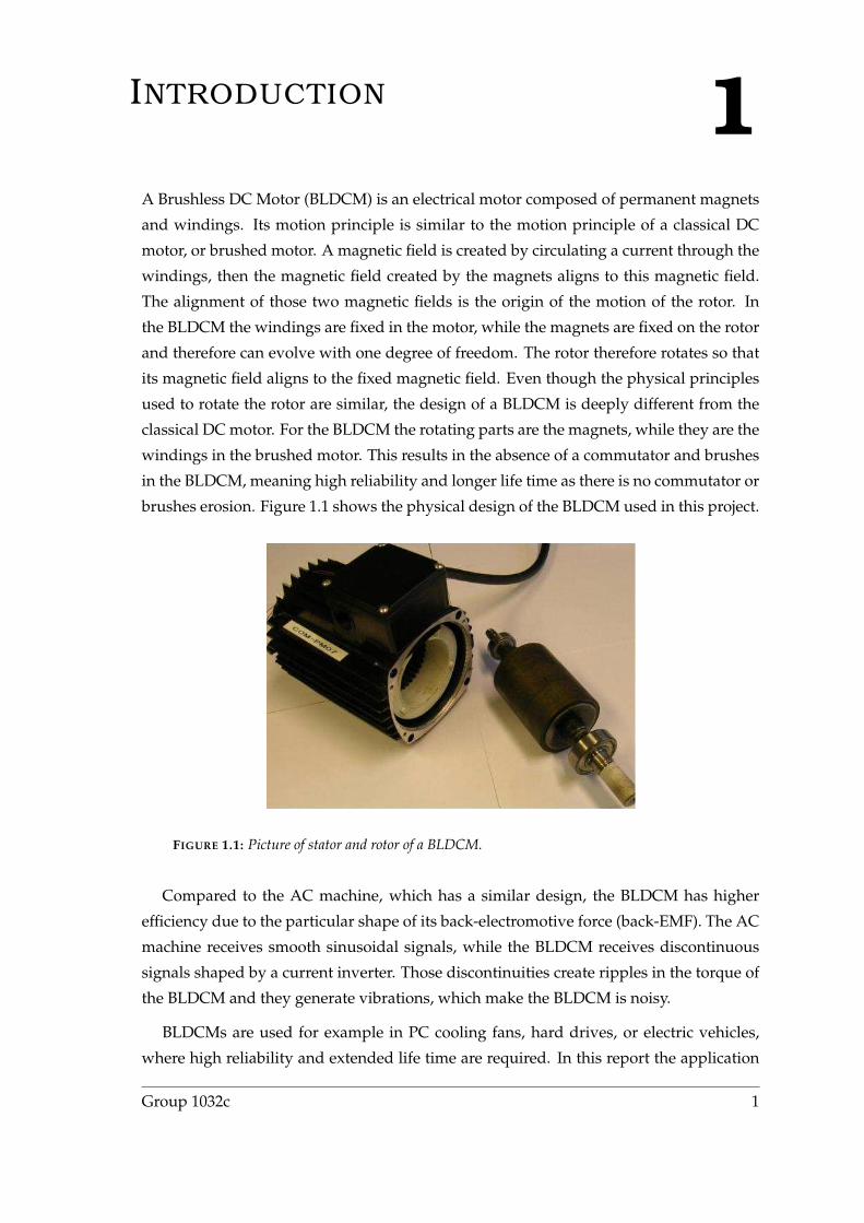
brushes erosion. Figure 1.1 shows the physical design of the BLDCM used in this project.
FIGURE 1.1: Picture of stator and rotor of a BLDCM.
Compared to the AC machine, which has a similar design, the BLDCM has higher
efficiency due to the particular shape of its back-electromotive force (back-EMF). The AC
machine receives smooth sinusoidal signals, while the BLDCM receives discontinuous
signals shaped by a current inverter. Those discontinuities create ripples in the torque of
the BLDCM and they generate vibrations, which make the BLDCM is noisy.
BLDCMs are used for example in PC cooling fans, hard drives, or electric vehicles,
where high reliability and extended life time are required. In this report the application
Group 1032c 1
that is considered is the BLDCM of a centrifugal pump, which can be used for instance
in waste water treatment or as submersible pump to extract water from sources. In this
type of application, it is particularly important to have high reliability as the access to the
pump for maintenance is generally restricted. A design robust to mechanical wear is also
an important asset knowing that the pump will run constantly at more than 70% of its
maximum speed. The tradeoff against this design is the need of an external controller. In
the brushed DC motor, the system commutator-brushes act like a mechanical controller,
since the rotaton of the commutator changes the brushes to which it is connected, creating
the required changes in current flows to move the rotor. As this does not exist on the
BLDCM, an external circuit is needed to generate the appropriate currents in the phases.
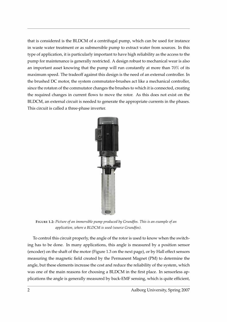
This circuit is called a three-phase inverter.
FIGURE 1.2: Picture of an immersible pump produced by Grundfos. This is an example of an
application, where a BLDCM is used (source Grundfos).
To control this circuit properly, the angle of the rotor is used to know when the switch-
ing has to be done. In many applications, this angle is measured by a position sensor
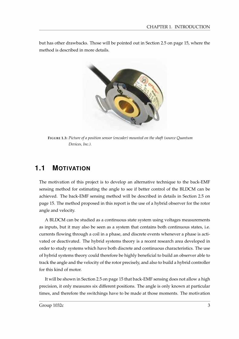
(encoder) on the shaft of the motor (Figure 1.3 on the next page), or by Hall effect sensors
measuring the magnetic field created by the Permanent Magnet (PM) to determine the
angle, but these elements increase the cost and reduce the reliability of the system, which
was one of the main reasons for choosing a BLDCM in the first place. In sensorless ap-
plications the angle is generally measured by back-EMF sensing, which is quite efficient,
2 Aalborg University, Spring 2007
CHAPTER 1. INTRODUCTION
but has other drawbacks. Those will be pointed out in Section 2.5 on page 15, where the
method is described in more details.
FIGURE 1.3: Picture of a position sensor (encoder) mounted on the shaft (source Quantum
Devices, Inc.).
1.1 MOTIVATION
The motivation of this project is to develop an alternative technique to the back-EMF
sensing method for estimating the angle to see if better control of the BLDCM can be
achieved. The back-EMF sensing method will be described in details in Section 2.5 on
page 15. The method proposed in this report is the use of a hybrid observer for the rotor
angle and velocity.
A BLDCM can be studied as a continuous state system using voltages measurements
as inputs, but it may also be seen as a system that contains both continuous states, i.e.
currents flowing through a coil in a phase, and discrete events whenever a phase is acti-
vated or deactivated. The hybrid systems theory is a recent research area developed in
order to study systems which have both discrete and continuous characteristics. The use
of hybrid systems theory could therefore be highly beneficial to build an observer able to
track the angle and the velocity of the rotor precisely, and also to build a hybrid controller
for this kind of motor.
It will be shown in Section 2.5 on page 15 that back-EMF sensing does not allow a high
precision, it only measures six different positions. The angle is only known at particular
times, and therefore the switchings have to be made at those moments. The motivation
Group 1032c 3
1.2. BACKGROUND
of designing an observer is that it would offer a better resolution of the angular position,
as the angle estimation would always be available. This would allow advanced control
methods to be used in the control of the BLDCM, giving the opportunity to improve the
performance of the motor.
The design of a hybrid observer is also motivated by a reduction of the number of
sensors used to estimate the angle. The back-EMF sensing method needs three sensors,
while the hybrid observer, at least in principle, has the capacity of estimating the angle
and the speed on basis of only one sensor, yielding a decrease in the cost and increase of
the reliability.
The hybrid observer would be based on measurements of the currents flowing thro-
ugh the windings, meaning that it would be able to work in any situation, while back-
EMF sensing requires that one of the winding’s current is null. Under certain conditions,
it can happen that currents flow all the time in all the windings, in which case the back-
EMF sensing method can not be applied.
1.2 BACKGROUND
Previous work showed the benefits from applying hybrid systems theory to the BLDCM.
A hybrid model of the BLDCM was derived, and proved to be accurate. The hybrid
model used throughout this report was firstly derived in [NP06] on basis of [Han06]
and [HB05]. A nonlinear hybrid observer for estimating the rotor angle and velocity was
designed on basis of this hybrid model. The parameters of the observer were found by an
optimization approach, which has shown to provide good results. The observer showed
encouraging accuracy, as it was able to estimate angle of the rotor within ±15, and the
error of the estimate of the angular velocity was within ±12 [rad · s−1]. This observer
was able to handle continuous changes in the angular velocity while keeping the same
precision in the estimates.
The hybrid observer was able to estimate angle and speed by using only two currents
sensors instead of three. A lot of efforts were made on reducing the computational de-
mand of the observer in order to have a system able to estimate online. Despite large
improvements at this level, the observer was still computationally too heavy, and only
offline tests have been realized.
4 Aalborg University, Spring 2007
CHAPTER 1. INTRODUCTION
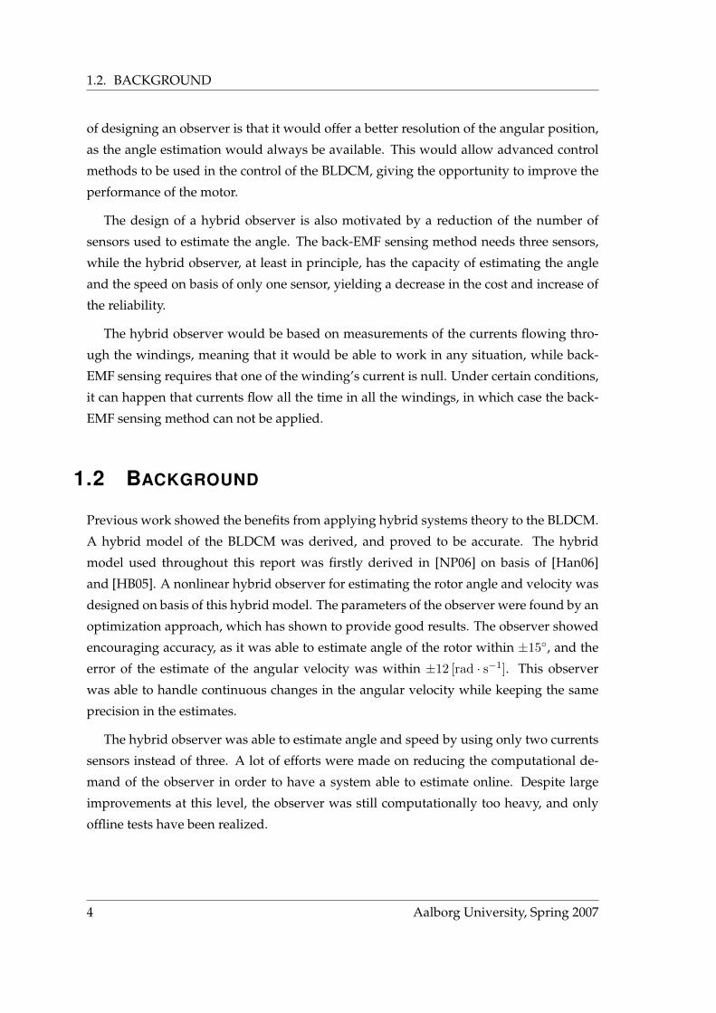
1.3 TEST SETUP
The test setup used during the project consisted of a motor connected to a power board
with a current inverter and sensors. The power board receives a PWM signal through
an optical link generated by a program running on dSpace R© . The control of the motor
was implemented in MATLAB R© using Simulink R© models which were compiled to the
dSpace R© interface to be sent to the target processor. The test setup is shown in Figure 1.4.
FIGURE 1.4: Picture of the test setup used in the project.
The important assumption in the project is that the considered range of speed is ωr ∈[500; 1000] [rpm]. This can be assumed as the goal of this project is to investigate the
possibility of using hybrid observer for controlling the BLDCM in pump application,
where the speed does not vary in the full range.
1.4 OBJECTIVES
Previous work has shown that a hybrid observer for the rotor angle and velocity can
be designed, and achieve sufficient accuracy. The observer was so far not implemented
online due to high computational demands.
In this project there are three main objectives, the first being to continue the work on
the hybrid observer. The observer designed in [NP06] has been shown to work correctly,
the objective is now to improve the precision of this observer. Firstly the structure of the
Group 1032c 5
1.5. REPORT OUTLINE
previous observer will be modified, i.e. any unused parts will be removed, and some
parts will be replaced by others providing a better accuracy of the estimates. Then, sev-
eral types of Evolutionary Algorithm (EA) will be applied to the optimization problem
of finding correct parameters for the observer. EA will be used as they seem to suit well
the optimization problem to solve, and therefore they could lead to better results than the
optimization procedure used in the previous work.
The second main task is to reduce the number of sensors used by the observer to
estimate the angle and the angular velocity. In this report, the use of only one current
measurement will be investigated. Tests of this observer will then be run to check that it
can work with real measurements.
The final task consists in testing both the single sensor observer and the double sensor
observer in a closed loop situation, i.e. when the observers are used to provide the angle
to a closed loop controller. This test will allow to check the behaviour of the observers in
real conditions, and it will show if the use of an observer is suitable to control a BLDCM.
In order to realize this final test, the observers must be able to estimate online on the
target processor. The Simulink R© implementations of the observers will be optimized so
that dSpace R© can compile and send them to the target processor. The computational
demand of the observers will be reduced in order to be able to estimate the angle and
the speed in real time. Then the final tests will be realized, and the results will allow to
conclude on the use of a hybrid observer in providing the angle to control a BLDCM.
1.5 REPORT OUTLINE
The report is organized the following way:
Chapter 2: Introduction to the BLDCM
This chapter presents preliminary knowledges to ease the understanding of the report.
The main concept of a BLDCM is presented. The current inverter used to control the cur-
rents in the BLDCM is then described. The main principles of the Pulse Width Modulation
(PWM) modulation are introduced, and the chosen control strategy for the motor is de-
fined. The back-EMF sensing method is presented. The equations for electrical and me-
chanical dynamics of the BLDCM are derived, and it is shown that only two differential
equations are needed to define the electrical dynamics of the motor.
Chapter 3: Hybrid model
Introduces the concept and mathematical formulation of a Hybrid System. A hybrid
6 Aalborg University, Spring 2007
CHAPTER 1. INTRODUCTION
automaton for the BLDCM is then derived. The differential equations corresponding
to each of the states of the hybrid automaton are expressed based on the differential
equations for the BLDCM derived in the previous chapter. The formal description of the
hybrid model derived is given. Finally, the results of a test of this model in [NP06] are
presented.
Chapter 4: Hybrid observer
This chapter is the description of a novel hybrid observer used in this project. The struc-
ture of the observer derived in [NP06] is modified in order to improve it. The new struc-
ture is presented, and the equations of the observer are expressed.
Chapter 5: Optimization of observer feedback
The principles of different classes of optimization algorithms suited for the determination
of observer’s parameters will be presented. The most suitable algorithms for the problem
considered will be selected. The different results will be compared and discussed, then
the best result of optimization will be kept to be used in the observer.
Chapter 6: Test of the observer
The observer derived in Chapter 4 will be tested using the new feedback parameters
found with the optimization methods of Chapter 5. This test will allow to check that the
behaviour of the observer is correct, and that its precision has been improved by its new
structure and feedback parameters.
Chapter 7: Single sensor observer
This chapter presents the reduction of the number of sensors to one current measurement
instead of two. First the two conditions required to be able to observe the BLDCM us-
ing only one current sensor will be expressed. Then it will be shown that both of those
conditions are fulfilled, and therefore changes will be made to the observer in order for
it to use one measurement. A test of this new observer will be realized to check that it
remains accurate with one sensor.
Chapter 8: Closed loop test of the observer
First, both observers are tested in Simulink R© using the model instead of the real BLDCM.
The observers will be used to provide the information of angle of the rotor to the com-
mutator. This test will allow to verify the functionality of the observers in closed loop
conditions. Having verified the performance of the observers in simulations, they will be
tested in closed loop conditions with the real motor. The results of those closed loop tests
will be analysed to determine the efficiency of the system using the observers.
Group 1032c 7

1.5. REPORT OUTLINE
Chapter 9: Conclusion
Results and achievements of the project will be discussed. Then, opportunities for future
work will be described.
8 Aalborg University, Spring 2007

2INTRODUCTION TO THEBLDCM
This chapter presents an overview of the BLDCM concept. The drive circuit of the BLDCM,
called three phase inverter, is described. The switching method using PWM modulation
is defined as well as the control strategy used to rotate the rotor. The back-EMF sens-
ing method is explained and its efficiency is discussed. The mathematical model of the
electrical and mechanical dynamics is then described. Those equations correspond to a
reduced model for the dynamics in the ab-frame, they were firstly derived in [NP06].
2.1 CONSTRUCTION
The advantages of the brushless design are mostly due to the fact that there is a limited
contact between elements inside the motor. This reduces friction, makes the motor more
robust to failures, and extends its lifetime. However this comes with a burden of a more
difficult control that has to be performed.
A BLDCM is a PM synchronous machine, which has uniformly wounded windings
and back-EMF of a trapezoidal shape. A possible configuration of a one pole pair magnet
motor is depicted in Figure 2.1 on the following page.
In case there is more than one magnet pole pair in the machine, the electrical angle (θe)
is not equal to the mechanical angle (θr). Electrical angle is the change in the magnetic
field, whereas the mechanical angle is the change in the rotor’s position. The relation
between these angles is given by equation 2.1, where Zp is a number of magnetic pole
pairs. This leads to relation 2.2 for the electrical angular velocity ωe, which is the time
derivative of the angle θe.
θe = Zpθr (2.1)
ωe = Zpωr (2.2)
A discontinuous six-step current inverter is used to generate the physical switching
between phases. The input signal to this inverter is shaped by a PWM device.
Group 1032c 9

2.2. THREE PHASE INVERTER
N
Si1s
i 2si3 s
i 3 si2s
i 1 s
Phase 1
Phase 1
P ha s
e 3
P ha s
e 3
Phas e 2
Phas e 2
θ
FIGURE 2.1: Uniform windings of a BLDCM with one magnetic pole pair [Chi05].
2.2 THREE PHASE INVERTER
The transition between direct current and the alternating current supplied to the motor is
carried out by switching MOSFET transistors. The design of such an inverter is depicted
in Figure 2.2.
T2
T5
T3
T6
T1
T4
Vcc
Va
Vb Vc
Neutral Potential
ia
icib
FIGURE 2.2: Electrical circuit of the 120 current inverter and a WYE-connected BLDCM.
The inverter is a six-step current inverter in which one of the phases is eventually
open circuited for 120 of the cycle. It is connected to the machine such that ias, ibs, ics are
the stator currents. Figure 2.3(a) on the facing page shows the idealized currents applied
10 Aalborg University, Spring 2007
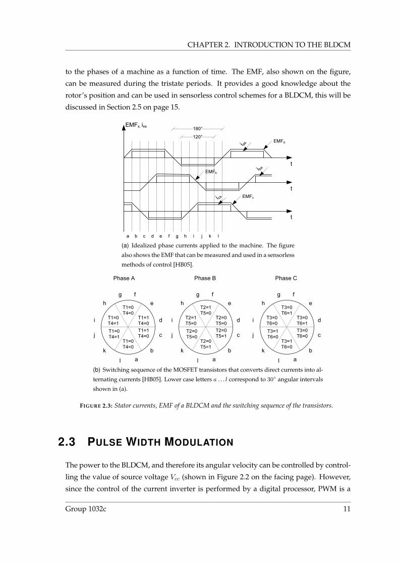
CHAPTER 2. INTRODUCTION TO THE BLDCM
to the phases of a machine as a function of time. The EMF, also shown on the figure,
can be measured during the tristate periods. It provides a good knowledge about the
rotor’s position and can be used in sensorless control schemes for a BLDCM, this will be
discussed in Section 2.5 on page 15.
t
a gfedcb h i lkji a s
i b s
i c st
t
EMFx, ixs
120°180°
EMFa
EMFb
EMFc
(a) Idealized phase currents applied to the machine. The figure
also shows the EMF that can be measured and used in a sensorless
methods of control [HB05].
T1=0T4=0
T1=0T4=0
T1=0T4=1
T1=1T4=0
T1=0T4=1
T1=1T4=0
ab
c
d
efg
h
i
j
kl
T2=1T5=0
T2=0T5=1
T2=1T5=0
T2=0T5=0
T2=0T5=0
T2=0T5=1
ab
c
d
efg
h
i
j
kl
T3=0T6=1
T3=1T6=0
T3=0T6=0
T3=0T6=1
T3=1T6=0
T3=0T6=0
ab
c
d
efg
h
i
j
kl
Phase A Phase B Phase C
(b) Switching sequence of the MOSFET transistors that converts direct currents into al-
ternating currents [HB05]. Lower case letters a . . . l correspond to 30 angular intervals
shown in (a).
FIGURE 2.3: Stator currents, EMF of a BLDCM and the switching sequence of the transistors.
2.3 PULSE WIDTH MODULATION
The power to the BLDCM, and therefore its angular velocity can be controlled by control-
ling the value of source voltage Vcc (shown in Figure 2.2 on the facing page). However,
since the control of the current inverter is performed by a digital processor, PWM is a
Group 1032c 11
2.3. Pulse Width Modulation
more efficient way of controlling the motor. The modulation is responsible for switch-
ing the transistors so that the amplitudes of the phase voltages have desired values. The
principle of the PWM modulation is to constantly switch between the supply voltage and
the ground, which explains why it is very suitable with digital processors as it is a binary
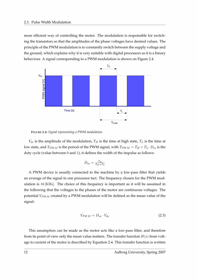
behaviour. A signal corresponding to a PWM modulation is shown on Figure 2.4.
PWM
signa
l [V]
Time [s]
Vdc
TH
TL
TPWM
FIGURE 2.4: Signal representing a PWM modulation.
Vdc is the amplitude of the modulation, TH is the time at high state, TL is the time at
low state, and TPWM is the period of the PWM signal, with TPWM = TH + TL. Din is the
duty cycle (value between 0 and 1), it defines the width of the impulse as follows:
Din = THTH+TL
A PWM device is usually connected to the machine by a low-pass filter that yields
an average of the signal in one processor tact. The frequency chosen for the PWM mod-
ulation is 16 [KHz]. The choice of this frequency is important as it will be assumed in
the following that the voltages to the phases of the motor are continuous voltages. The
potential VPWM created by a PWM modulation will be defined as the mean value of the
signal:
VPWM = Din · Vdc (2.3)
This assumption can be made as the motor acts like a low-pass filter, and therefore
from its point of view only the mean value matters. The transfer functionH(s) from volt-
age to current of the motor is described by Equation 2.4. This transfer function is written
12 Aalborg University, Spring 2007
CHAPTER 2. INTRODUCTION TO THE BLDCM
on basis of Figure 2.2 on page 10, which shows that a phase of the motor is equivalent to
an inductance and a resistor connected in serial.
H(s) =1rs
1 + sLsrs
(2.4)
With rs and Ls the resistance and the inductance of a phase respectively. It will be
estimated later on that rs = 3.8 [Ω] and Ls = 0.0135 [H]. The cut-off frequency fc is de-
fined as fc = rs2πLs
= 44.8 [Hz]. After passing through this filter, the harmonic at 16 [KHz]
undergoes an attenuation of −46dB, and thus it is acceptable to consider only the mean
value of the PWM signal.
The higher the PWM frequency, the higher the attenuation, however in this case it is
not possible to use a frequency larger than 16 [KHz] for two reasons. Firstly, there is a
dead-band time of 1µs. A dead-band time is a short period of time during which the
transistors are all switched off before some of them are switched on. This is done as
the transistors do not switch off instantaneously, and this time allow them to close com-
pletely before the others switch on, avoiding short circuits. In this report, the influence of
the dead-band can be neglected, but in case the PWM frequency would be higher, Equa-
tion 2.5 would not be a valid approximation for the phase’s voltage. The second reason is
that the transistors in the three phase inverter are large, so they cannot switch at too high
frequency.
As it is represented on Figure 2.2 on page 10, each of the legs of the inverter has two
transistors to control the current flow in the phases. The higher Din the bigger voltage
drop is created. The duty cycle applied to the higher transistor (T1, T2 or T3) is calledDH
and the lower transistor’s (T4, T5 or T6) duty cycle is called DL. The voltage to a phase
is due to the superposition of two PWM modulations. Using Equation 2.3 on the facing
page, the potential to phase x, Vx is defined as follows:
Vx = DHVcc+ +DLVcc− (2.5)
Where Vcc+ and Vcc− are the positive and negative supply potentials respectively. The
supply voltage Vcc to the current inverter is therefore defined as Vcc = Vcc+ − Vcc−. The
transitors of one leg of the inverter should never be open at the same time, otherwise
it would create a short circuit. In order to avoid any short circuit, the transistors are
complementary, i.e. when one is open the other one is closed. This means that there is
a relation between DH and DL: DL = 1 − DH . Equation 2.5 on the previous page is
Group 1032c 13

2.4. CONTROL STRATEGY
rewritten as follows:
Vx = DHVcc+ + (1−DH)Vcc− (2.6)
2.4 CONTROL STRATEGY
There are several types of control strategies that can be chosen. Each of them has an effect
on the neutral node potential (Vn). In the report, the PWM-PWM-Tristate modulation
is used. In this modulation, one phase is off, and the other two phases, x and y, are
controlled with a PWM modulation. One phase receives a modulation with Din as duty
cycle, and the second receive a modulation with 1−Din as duty cycle. From Equation 2.6,
inputs to the active phases x and y at a time are
vx = DinVcc+ + (1−Din)Vcc−
vy = (1−Din)Vcc+ +DinVcc−(2.7)
Using Equations 2.7, the voltage drop through the phases is expressed as
vx − vy = DinVcc+ + (1−Din)Vcc− − (1−Din)Vcc+ +DinVcc−
= Vcc+(2Din − 1)− Vcc−(2Din − 1)
= (2Din − 1)Vcc
(2.8)
As it is shown by Equation 2.8, the advantage of this type of control is that the voltage
drop to the phases can vary from −Vcc+ to Vcc+.
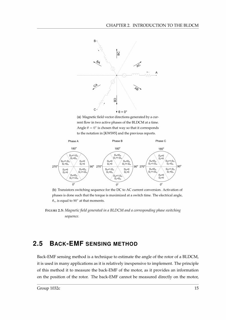
Figure 2.5(a) on the next page shows how the magnetic field in the BLDCM is gener-
ated by putting currents through proper phases. The following notation is used, "XY "
means that phase X is receiving a PWM signal with duty cycle Din, and phase Y with
duty cycle 1 − Din. Based on this figure, the switching sequence for the transistors can
be determined. It is presented in Figure 2.5(b) on the facing page. The switching is done
so that the torque is maximized, i.e. at a switch the electrical angle between the magnetic
field generated by the coils and the magnetic field created by the PM is 90.
14 Aalborg University, Spring 2007
CHAPTER 2. INTRODUCTION TO THE BLDCM
BC
CB
(a) Magnetic field vector directions generated by a cur-
rent flow in two active phases of the BLDCM at a time.
Angle θ = 0 is chosen that way so that it corresponds
to the notation in [KWS95] and the previous reports.
DH=0DL=0
DH=1-DinDL=Din
DH=DinDL=1-Din
DH=1-DinDL=Din
DH=0DL=0
DH=DinDL=1-Din
Phase A Phase B
DH=DinDL=1-Din
DH=DinDL=1-Din
DH=0DL=0
DH=1-DinDL=Din
DH=0DL=0
DH=1-DinDL=Din
Phase C
DH=DinDL=1-Din
DH=DinDL=1-Din
DH=1-DinDL=Din
DH=0DL=0
DH=1-DinDL=Din
DH=0DL=0
90o 90o90o
180o180o180o
270o 270o 270o
0o 0o0o
(b) Transistors switching sequence for the DC to AC current conversion. Activation of
phases is done such that the torque is maximized at a switch time. The electrical angle,
θe, is equal to 90 at that moments.
FIGURE 2.5: Magnetic field generated in a BLDCM and a corresponding phase switching
sequence.
2.5 BACK-EMF SENSING METHOD
Back-EMF sensing method is a technique to estimate the angle of the rotor of a BLDCM,
it is used in many applications as it is relatively inexpensive to implement. The principle
of this method it to measure the back-EMF of the motor, as it provides an information
on the position of the rotor. The back-EMF cannot be measured directly on the motor,
Group 1032c 15
2.6. DYNAMICS OF THE BLDCM
therefore it is sensed through the voltage of the tristated phase [PC05].
In case there is no current in a phase, the inductance and resistor of the phase have no
influence on the terminal voltage, and only the back-EMF remains, therefore by measur-
ing the voltage to the tristated phase (assumed to have no current through it) the back-
EMF is measured. As shown on Figure 2.3(a) on page 11, the back-EMF has a periodic
shape, and it crosses zero when the permanent magnet is aligned to a phase. Zero cross-
ing detection is used to detect those alignments, and when a zero crossing is detected,
the correct switchings are made.
This method does not allow advanced control method to be used, as the position of
the rotor is only known at certain moments. Better performance could be obtained if the
measure of the angle would be always available, for instance torque control techniques
could be used to reduce the torque ripples, as it is done in [HLL95].
It is assumed that the current through the tristated phase is null, but the current thro-
ugh a coil does not stop immediately, some current is drained during a certain time after
tristating. In certain situations, a drain current can circulate through the phase during
the whole tristate period, in that case the back-EMF method is not efficient to estimate
the rotor position. This type of situation can happen at high speed, and in that case the
coil has very short time to discharge its energy before the phase is switch on again. This
can also happen in case the currents are high, which means that the drain current remains
longer in the phase.
2.6 DYNAMICS OF THE BLDCM
In order to simplify the dynamical equations of the motor, several assumptions are made.
Those are general assumptions that are usually made when modelling a 3-phase balanced
machine.
• The BLDCM is balanced, which means that there is 120 (electrical) between the
stator windings, and that they have equal ohmic resistance and inductance. The
values of the resistance and inductance are assumed constants.
• The influence of the iron is neglected, i.e. the magnetic permeability of the iron is
infinite, magnetic fields only exists in the air gap between stator and rotor.
• The rotor is perfectly round and the air gap uniform. The flux lines are radial in the
air gap, and the magnetic system is assumed linear.
16 Aalborg University, Spring 2007
CHAPTER 2. INTRODUCTION TO THE BLDCM
In the following sections the equations for electrical and mechanical dynamics used in
this report are presented. Those equations were derived for the first time in [NP06]. The
torque equation uses only two phase currents instead of three. In the previous work volt-
age equations were transformed to qd-frame where they were simplified and transformed
back to the abc-frame. In this report, a new way of deriving the electrical dynamics with-
out transformation is used. Using this description for the dynamics, the system has a
form which is easily understandable due to the fact that it uses the input voltages to the
phases and the phase currents directly. Those are the inputs and the measurements re-
spectively. No transformation is required inside the MATLAB R© /Simulink R© model, and
only two differential equations are sufficient to describe the dynamics of the motor. Con-
sidering that the goal is to implement the observer on-line, and that the observer uses
this model, the lighter (in terms of computation) is the model, the lighter is the observer,
and therefore the greater is the chance of being able to run the observer on-line.
2.6.1 ELECTRICAL DYNAMICS
The voltage drops across the phases in stator reference frame are described by Equa-
tion 2.9, which is written on the basis of Figure 2.2 on page 10. Note that the last term on
the right side of the equation corresponds to the back-EMF.
vabcs = Lsd
dtiabcs︸ ︷︷ ︸
Inductance
+ Rsiabcs︸ ︷︷ ︸Resistance
+(d
dθeλ′
m)ωe︸ ︷︷ ︸Back−EMF
(2.9)
Where vabcs =
vas
vbs
vcs
=
Vas − Vn
Vbs − Vn
Vcs − Vn
= Vabcs − Vn, Vn being the potential at the
neutral node, Vabcs the vector of input voltages, and iabcs =[ias ibs ics
]T, the vector
of currents trough the phases. Applying Kirchoff’s law on the neutral node defines a
constraint on these currents:
ias + ibs + ics = 0 (2.10)
Ls =
Lls + Lms −1
2Lms −12Lms
−12Lms Lls + Lms −1
2Lms
−12Lms −1
2Lms Lls + Lms
is the inductance matrix, Lls is the leak-
age inductance, and Lms is the magnetizing inductance.
Group 1032c 17
2.6. DYNAMICS OF THE BLDCM
The resistance matrix has the form of Rs =
rs 0 0
0 rs 0
0 0 rs
, where rs is the resistance
of a stator winding.
λ′m is the vector of the stator flux linkages created by the permanent magnet, which
is a periodic function of the rotor position. A BLDCM is generally designed to have a
symmetric trapezoidal back-EMF, therefore λ′m can be decomposed in a series of odd
harmonics:
λ′m = λ′m
∞∑n=1
N2n−1
sin((2n− 1)θe)
sin((2n− 1)(θe − 2π3 ))
sin((2n− 1)(θe + 2π3 ))
(2.11)
With λ′m being the magnitude of the first harmonic, and N2n−1 the magnitude of the
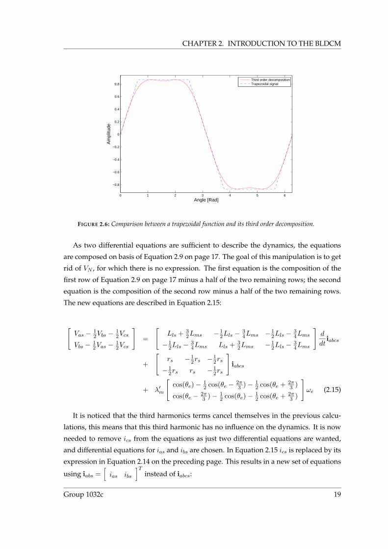
nth odd harmonic relative to the fundamental. The comparison between a trapezoidal
function and its third order decomposition is shown in Figure 2.6 on the facing page,
it is noticed that the first and third harmonics should be enough to describe the flux
linkages. In the following, the flux linkages will always be taken as their third order
decomposition. More harmonics can be considered if the model becomes inaccurate due
to this assumption.
λ′m = λ′m
sin(θe) +N3 sin(3θe)
sin(θe − 2π3 ) +N3 sin(3θe)
sin(θe + 2π3 ) +N3 sin(3θe)
(2.12)
Using the previous equation, the back-EMF can be expressed:
(d
dθeλ′
m)ωe = λ′m
cos(θe) + 3N3 cos(3θe)
cos(θe − 2π3 ) + 3N3 cos(3θe)
cos(θe + 2π3 ) + 3N3 cos(3θe)
ωe (2.13)
The constraints on the currents described by Equation 2.10 on the previous page pro-
vide an important information. It means that the currents evolve on a two-dimensional
manifold, and therefore only two differential equations are needed to describe completely
the electrical dynamics of the motor. Equation 2.10 on the preceding page can be rewrit-
ten so that ics is a function of ias and ibs:
ics = −ias − ibs (2.14)
18 Aalborg University, Spring 2007
CHAPTER 2. INTRODUCTION TO THE BLDCM
0 1 2 3 4 5 6
−0.8
−0.6
−0.4
−0.2
0
0.2
0.4
0.6
0.8
Angle [Rad]
Am
plitu
de
Third order decompositionTrapezoidal signal
FIGURE 2.6: Comparison between a trapezoidal function and its third order decomposition.
As two differential equations are sufficient to describe the dynamics, the equations
are composed on basis of Equation 2.9 on page 17. The goal of this manipulation is to get
rid of VN , for which there is no expression. The first equation is the composition of the
first row of Equation 2.9 on page 17 minus a half of the two remaining rows; the second
equation is the composition of the second row minus a half of the two remaining rows.
The new equations are described in Equation 2.15:
[Vas − 1
2Vbs − 12Vcs
Vbs − 12Vas − 1
2Vcs
]=
[Lls + 3
2Lms −12Lls − 3
4Lms −12Lls − 3
4Lms
−12Lls − 3
4Lms Lls + 32Lms −1
2Lls − 34Lms
]d
dtiabcs
+
[rs −1
2rs −12rs
−12rs rs −1
2rs
]iabcs
+ λ′m
[cos(θe)− 1
2 cos(θe − 2π3 )− 1
2 cos(θe + 2π3 )
cos(θe − 2π3 )− 1
2 cos(θe)− 12 cos(θe + 2π
3 )
]ωe (2.15)
It is noticed that the third harmonics terms cancel themselves in the previous calcu-
lations, this means that this third harmonic has no influence on the dynamics. It is now
needed to remove ics from the equations as just two differential equations are wanted,
and differential equations for ias and ibs are chosen. In Equation 2.15 ics is replaced by its
expression in Equation 2.14 on the preceding page. This results in a new set of equations
using iabs =[ias ibs
]Tinstead of iabcs:
Group 1032c 19
2.6. DYNAMICS OF THE BLDCM
[Vas − 1
2Vbs − 12Vcs
Vbs − 12Vas − 1
2Vcs
]=
[32Lls + 9
4Lms 0
0 32Lls + 9
4Lms
]d
dtiabs +
[32rs 0
0 32rs
]iabs
+ λ′m
[cos(θe)− 1
2 cos(θe − 2π3 )− 1
2 cos(θe + 2π3 )
cos(θe − 2π3 )− 1
2 cos(θe)− 12 cos(θe + 2π
3 )
]ωe (2.16)
The last term in the previous equation can be simplified by using the trigonometrical
property cos(a+ b) = cos(a) cos(b)− sin(a) sin(b):
[cos(θe)− 1
2 cos(θe − 2π3 )− 1
2 cos(θe + 2π3 )
cos(θe − 2π3 )− 1
2 cos(θe)− 12 cos(θe + 2π
3 )
]=
[32 cos(θe)
−34 cos(θe) + 3
√3
4 sin(θe)
]
=
[32 0
−34
3√
34
][cos(θe)
sin(θe)
]
The previous expression is used in Equation 2.16 to provide a reduced form of the
equations:
[Vas − 1
2Vbs − 12Vcs
Vbs − 12Vas − 1
2Vcs
]=
[32Lls + 9
4Lms 0
0 32Lls + 9
4Lms
]d
dtiabs +
[32rs 0
0 32rs
]iabs
+ λ′m
[32 0
−34
3√
34
][cos(θe)
sin(θe)
]ωe (2.17)
Equation 2.17 is then multiplied with 23 and rearranged:
[Ls 0
0 Ls
]d
dtiabs = −
[rs 0
0 rs
]iabs − λ′m
[1 0
−12
√3
2
][cos(θe)
sin(θe)
]ωe
+
[23 −1
3 −13
−13
23 −1
3
]Vabcs (2.18)
With Ls = Lls + 32Lms being the equivalent inductance of a phase. Equation 2.18 is
rewritten to find the final expression of the electrical dynamics of the BLDCM:
20 Aalborg University, Spring 2007
CHAPTER 2. INTRODUCTION TO THE BLDCM
d
dtiabs = − rs
Lsiabs −
λ′mLs
[1 0
−12
√3
2
]︸ ︷︷ ︸
M′′
[cos(θe)
sin(θe)
]ωe
+1Ls
[23 −1
3 −13
−13
23 −1
3
]︸ ︷︷ ︸
M′
Vabcs (2.19)
The current ics is not present in the final electrical dynamics, if it is needed in the im-
plementation it can be easily computed using its expression in Equation 2.14 on page 18.
2.6.2 MECHANICAL DYNAMICS
The equation of the torque produced by the BLDCM is derived from the energy of the
magnetic system:
Te = Zp
(d
dθeλ′
m
)T
iabcs (2.20)
Replacing ics by its expression in Equation 2.14 on page 18 and using Equation 2.13 on
page 18 leads to a new expression for the torque:
Te = Zpλ′m
[cos(θe)− cos(θe + 2π
3 )
cos(θe − 2π3 )− cos(θe + 2π
3 )
]T
iabs (2.21)
Then, using the trigonometric property cos(a + b) = cos(a) cos(b) − sin(a) sin(b), the
torque is rewritten:
Te = Zpλ′m
([32
√3
2
0√
3
][cos(θe)
sin(θe)
])T
iabs (2.22)
The motion of the motor is described by the following differential equation:
Jd
dtωr = Te −Bmωr + TL (2.23)
Where J is the moment of inertia of the rotor and load, Bm the damping coefficient of the
motor, and TL the torque produced by the load, which can be either positive or negative.
Multiplying Equation 2.23 with Zp allows to find the equation of motion of the BLDCM:
Group 1032c 21

2.7. CONCLUSION
Jd
dtωe = ZpTe −Bmωe + ZpTL (2.24)
The expression of Te in Equation 2.22 on the previous page is inserted in Equation 2.24
to find the final description of the mechanical dynamics:
Jd
dtωe = Z2
pλ′m
([32
√3
2
0√
3
][cos(θe)
sin(θe)
])T
iabs −Bmωe + ZpTL (2.25)
The BLDCM is a nonlinear system as there is are product between variables in the
electrical dynamics and the mechanical dynamics.
2.7 CONCLUSION
In this chapter the preliminary knowledge related to the project was presented. This
knowledge should allow the reader to understand the concepts presented in the follow-
ing parts of the report. New mathematical equations describing the physical behaviour
of the motor were presented. The qd-transformation is not necessary in this description,
which should enhance performance of the model and observer.
22 Aalborg University, Spring 2007

3HYBRID MODEL
This chapter describes the hybrid model used for the BLDCM. Firstly, a recently devel-
oped, compact definition of a hybrid system is given. Later, it will be shown how the
final hybrid automaton was derived from a general hybrid automaton for the BLDCM,
using knowledge of the control strategy in order to reduce the number of states and tran-
sitions. The scope of the project is limited to only one rotating direction. This limitation
is not very crucial as the BLDCM is used as a centrifugal pump motor. Adding the other
rotating direction can easily be done through symmetry. The rotating direction consid-
ered here will be ωe > 0. The continuous time equations corresponding to the states of
the hybrid automaton will be expressed on basis of the equations found in the previous
chapter. The formal description of the model will be written based on the definition of a
hybrid system given in Section 3.1.
3.1 DEFINITION OF A HYBRID SYSTEM
The hybrid systems theory is a relatively new field of research and therefore there is a
lot of work in the academic world concentrating on developing its theoretical backgro-
und. There are several definitions used for describing a hybrid system. In this report the
definition proposed in [ALB06] is used.
A hybrid system is a system that encounters abrupt changes in its dynamical be-
haviour and therefore cannot be described by purely continuous equations of dynamics.
The system can be considered as a combination of a continuous system, that is switched
by Finite State Automaton (FSA). Figure 3.1 on the following page shows the block dia-
gram and the relations between the continuous and discrete part of the system.
Definition 1
A hybrid system is defined as an 8-tuple:
H = (Q, X, U, Y,E,F ,G, T ) (3.1)
where
• Q = 1, 2, . . . , s ⊂ Z+ is the set of location indexes with cardinal number s,
• X = x|x ∈ Xq : q ∈ Q,Xq ⊆ Rnq is the continuous state-space with dimension
Group 1032c 23

3.2. HYBRID AUTOMATON
Switched Continuous System
Finate State Automaton
Continuous Input (u)
Events (e)
Location (q)Cont. State
(x)Cont. Input
(u)
Continuous Output (yc)
Discrete Output (yd)
FIGURE 3.1: Hybrid System can be represented as a combination of Switched Continuous
System and Finite State Automaton [EFS02].
nq∈Q ∈ Z+,
• U = u|u ∈ Uq : q ∈ Q,Uq ⊆ Rmq is the continuous input-space with dimension
mq∈Q ∈ Z+,
• Y = y|y ∈ Yq : q ∈ Q,Yq ⊆ Rpq is the continuous output-space with dimension
pq∈Q ∈ Z+,
• E =e|e ∈ 2Σ
is the set of possible input/output event labels, where Σ is an
appropriate set of labels,
• F : Q×X × U → X is the forcing function on the continuous state-space,
• G : Q×X × U → Y is a continuous output map,
• T : Q×X × U × E → Q×X × E is a transition map.
The continuous forcing function F , output mapping G and discrete transition map Tdepend on the discrete location, continues states and inputs, while events e affect only
the discrete dynamics.
3.2 HYBRID AUTOMATON
The hybrid automaton for a phase of the BLDCM described in [HB05] has four discrete
states depending on the inputs from the inverter and the current that flows through it.
This automaton is used as a basis for building the new reduced hybrid automaton for the
BLDCM used throughout this report.
24 Aalborg University, Spring 2007
CHAPTER 3. HYBRID MODEL
• The phase is said to be passive if no current flows trough it.
• The phase is said to be active if one of its two control transistors is conducting.
These transistors are in Figure 2.2 on page 10, T1 and T4 for phase A, T2 and T5
for phase B, and T3 and T6 for phase C.
• The phase is said to be in drain state if one of its two free wheel diodes is conduct-
ing. There are two cases depending on the sign of the current flowing trough the
phase, if the current is positive it is called positive drain, if it is negative negative
drain.
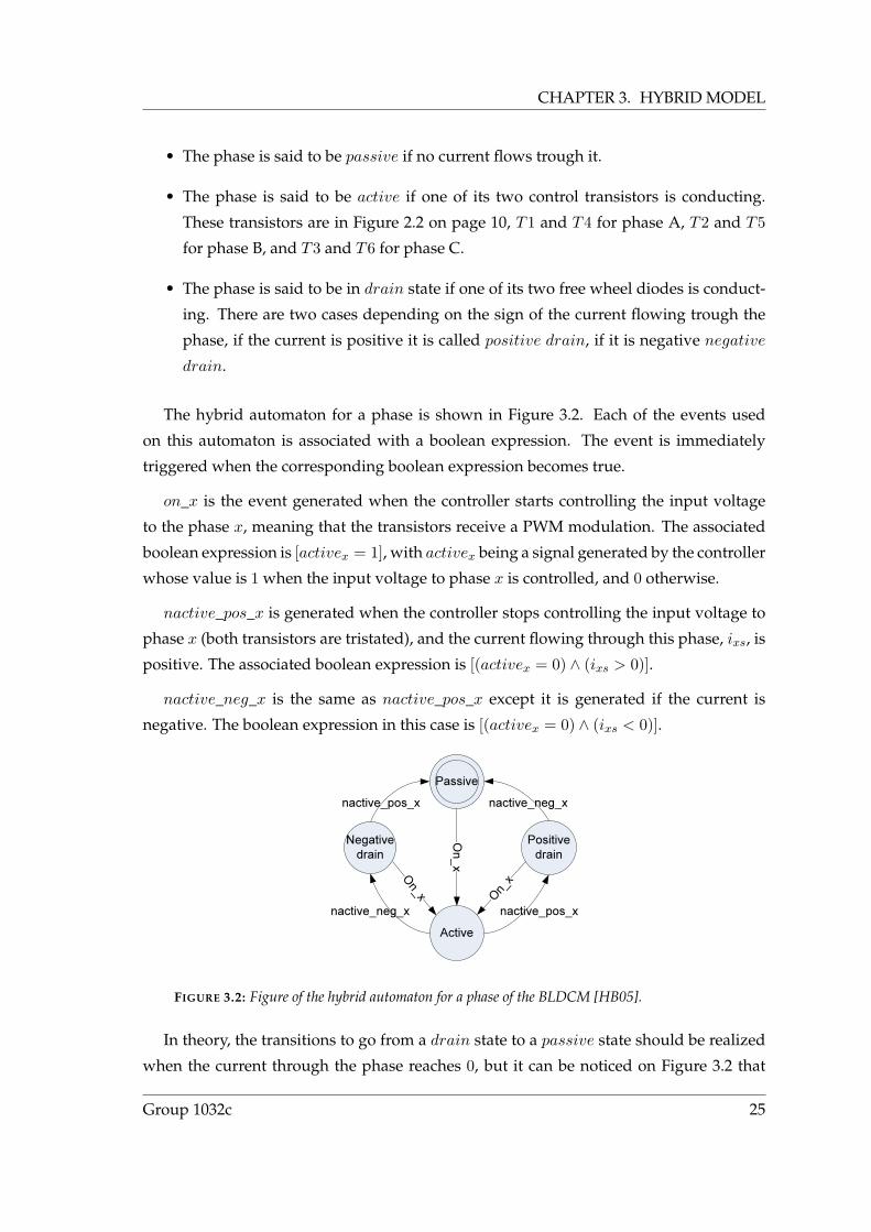
The hybrid automaton for a phase is shown in Figure 3.2. Each of the events used
on this automaton is associated with a boolean expression. The event is immediately
triggered when the corresponding boolean expression becomes true.
on_x is the event generated when the controller starts controlling the input voltage
to the phase x, meaning that the transistors receive a PWM modulation. The associated
boolean expression is [activex = 1], with activex being a signal generated by the controller
whose value is 1 when the input voltage to phase x is controlled, and 0 otherwise.
nactive_pos_x is generated when the controller stops controlling the input voltage to
phase x (both transistors are tristated), and the current flowing through this phase, ixs, is
positive. The associated boolean expression is [(activex = 0) ∧ (ixs > 0)].
nactive_neg_x is the same as nactive_pos_x except it is generated if the current is
negative. The boolean expression in this case is [(activex = 0) ∧ (ixs < 0)].
Active
Negative drain
Positive drain
Passive
On_x
On_x
O n_ x
nactive_pos_x nactive_neg_x
nactive_pos_xnactive_neg_x
FIGURE 3.2: Figure of the hybrid automaton for a phase of the BLDCM [HB05].
In theory, the transitions to go from a drain state to a passive state should be realized
when the current through the phase reaches 0, but it can be noticed on Figure 3.2 that
Group 1032c 25
3.2. HYBRID AUTOMATON
these transitions are realized when the sign of the current changes. In the implementa-
tion, the current never reaches exactly zero at any given sample instant, therefore a zero
crossing detection is used instead of a zero detection.
The global hybrid automaton for the BLDCM is composed of three phase’s automa-
tons in parallel, one for each phase. Each phase’s automaton is composed of 4 states,
therefore the composition of these three automatons gives an automaton with 43 = 64
states, as derived in [HB05]. Such a large number of discrete states is difficult to consider
in practice, and thus the automaton will be reduced in the following.
Knowing the control strategy used, which is described by Figure 2.5(b) on page 15, a
large number of the states can be omitted in the final hybrid automaton, as they are not
reachable. The states that are in the final automaton must fulfill the following require-
ments:
• Two phases are active.
• One phase is either passive, positive drain, or negative drain.
The transitions making the motor turn in the direction ωe < 0 cannot be realized under
the chosen control strategy, as only the rotating direction ωe > 0 is considered, these
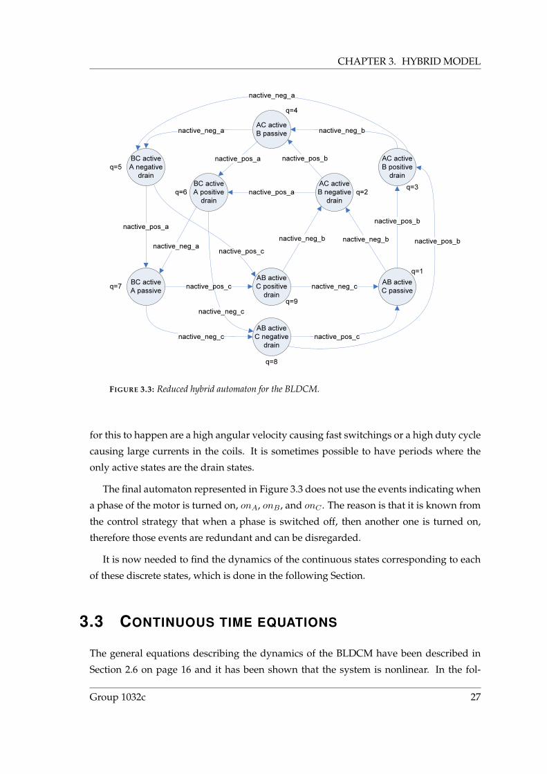
transitions are therefore omitted in the final automaton. The final automaton is shown
on Figure 3.3 on the facing page, where the value of q is the location index corresponding
to the state.
The final hybrid automaton for the BLDCM is composed of 9 different states. There
are no deadlocks in this automaton as the events that trigger the transitions are generated
outside the automaton. The automaton has a cyclic shape, which is due to the rotating
behaviour of the system itself.
It is noticed that the control strategy chosen is included in the automaton. A brief ana-
lysis of the automaton allows to find the switching sequence for the phases represented
by Figure 2.5(b) on page 15: ABactive→ ACactive→BCactive→ ABactive→ . . . But
the automaton is composed of more states than only the ones from the control sequence,
there are also the drain states.
Transitions are possible from one drain state directly to another drain state without
passing through a state where only two phases are conducting. This happens when one
or more of the coils do not have enough time to discharge completely before becoming
active again, meaning the currents are too large or the switchings are too fast. Reasons
26 Aalborg University, Spring 2007
CHAPTER 3. HYBRID MODEL
AB activeC passive
AC activeB passive
BC activeA passive
AB activeC positive
drain
AB activeC negative
drain
BC activeA negative
drainBC activeA positive
drain
AC activeB positive
drainAC activeB negative
drain
nactive_neg_a nactive_neg_b
nactive_pos_a nactive_pos_b
nactive_neg_b
nactive_pos_b
nactive_neg_c
nactive_pos_cnactive_neg_c
nactive_neg_a
nactive_pos_a
nactive_pos_c
nactive_pos_a
nactive_neg_b nactive_pos_b
nactive_neg_a
nactive_neg_c
nactive_pos_c
q=1
q=3q=2
q=4
q=5
q=6
q=7
q=8
q=9
FIGURE 3.3: Reduced hybrid automaton for the BLDCM.
for this to happen are a high angular velocity causing fast switchings or a high duty cycle
causing large currents in the coils. It is sometimes possible to have periods where the
only active states are the drain states.
The final automaton represented in Figure 3.3 does not use the events indicating when
a phase of the motor is turned on, onA, onB , and onC . The reason is that it is known from
the control strategy that when a phase is switched off, then another one is turned on,
therefore those events are redundant and can be disregarded.
It is now needed to find the dynamics of the continuous states corresponding to each
of these discrete states, which is done in the following Section.
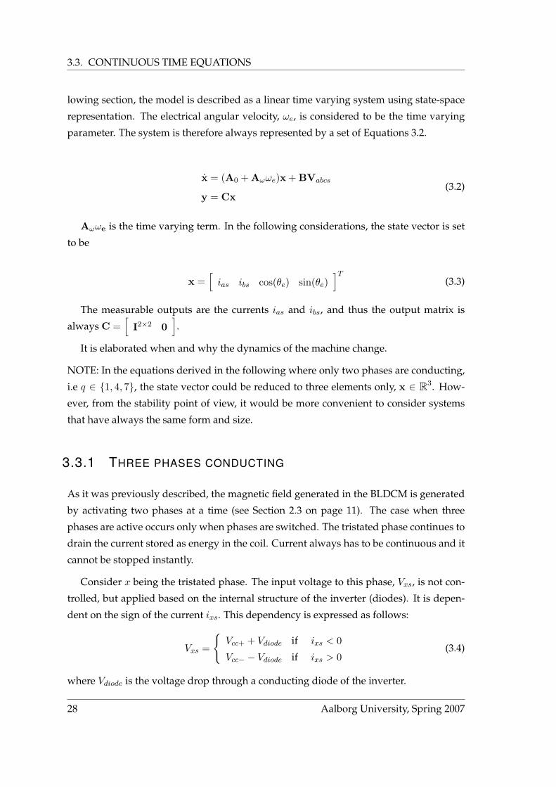
3.3 CONTINUOUS TIME EQUATIONS
The general equations describing the dynamics of the BLDCM have been described in
Section 2.6 on page 16 and it has been shown that the system is nonlinear. In the fol-
Group 1032c 27
3.3. CONTINUOUS TIME EQUATIONS
lowing section, the model is described as a linear time varying system using state-space
representation. The electrical angular velocity, ωe, is considered to be the time varying
parameter. The system is therefore always represented by a set of Equations 3.2.
x = (A0 + Aωωe)x + BVabcs
y = Cx(3.2)
Aωωe is the time varying term. In the following considerations, the state vector is set
to be
x =[ias ibs cos(θe) sin(θe)
]T(3.3)
The measurable outputs are the currents ias and ibs, and thus the output matrix is
always C =[
I2×2 0].
It is elaborated when and why the dynamics of the machine change.
NOTE: In the equations derived in the following where only two phases are conducting,
i.e q ∈ 1, 4, 7, the state vector could be reduced to three elements only, x ∈ R3. How-
ever, from the stability point of view, it would be more convenient to consider systems
that have always the same form and size.
3.3.1 THREE PHASES CONDUCTING
As it was previously described, the magnetic field generated in the BLDCM is generated
by activating two phases at a time (see Section 2.3 on page 11). The case when three
phases are active occurs only when phases are switched. The tristated phase continues to
drain the current stored as energy in the coil. Current always has to be continuous and it
cannot be stopped instantly.
Consider x being the tristated phase. The input voltage to this phase, Vxs, is not con-
trolled, but applied based on the internal structure of the inverter (diodes). It is depen-
dent on the sign of the current ixs. This dependency is expressed as follows:
Vxs =
Vcc+ + Vdiode if ixs < 0
Vcc− − Vdiode if ixs > 0(3.4)
where Vdiode is the voltage drop through a conducting diode of the inverter.
28 Aalborg University, Spring 2007

CHAPTER 3. HYBRID MODEL
When the currents are flowing through all three phases, the electrical dynamics are
described by Equation 2.19 on page 21. The system is brought to a linear time varying
system representation of the form 3.2 on the preceding page, where the state vector is
given in Equation 3.3 on the facing page.
A0 =
[− rs
LsI2×2 0
0 0
], Aω =
[0 −λ′m
LsM′′
0 J
], J =
[0 −1
1 0
]and B =
[1
LsM′
0
]
and
M′ =
[23 −1
3 −13
−13
23 −1
3
], M′′ =
[1 0
−12
√3
2
]
The mechanical dynamics are described by Equation 2.24 on page 22, which is used to
compute the time-varying parameter ωe.
3.3.2 TWO PHASES CONDUCTING
This is the default situation from the control point of view. The tristated phase, x, does
not drain any current, ixs = 0, and the currents through the conducting phases y and z
are constrained by iys = −izs. This corresponds to rewriting of Equation 2.10 on page 17
when one phase current is 0. The equations vary depending on which phase is off, there-
fore they have to be analyzed separately.
Phase C not conducting The first case to be analysed is when ics = 0 ⇒ ias = −ibs.
The system can be expressed using only one differential equation. It can be derived
from Equation 2.19 on page 21. The voltage in the node that is not controlled, Vc, is
governed by internal dynamics of the motor, i.e. the back-EMF voltage inducted by the
rotor movement. To remove this voltage from the equation, a small trick is used and the
difference ddt(ias − ibs) is analysed.
d
dt(ias − ibs) = − rs
Ls(ias − ibs)−
λ′mLs
[32 −
√3
2
] [ cos(θe)
sin(θe)
]ωe
+1Ls
[1 −1 0
]Vabcs
(3.5)
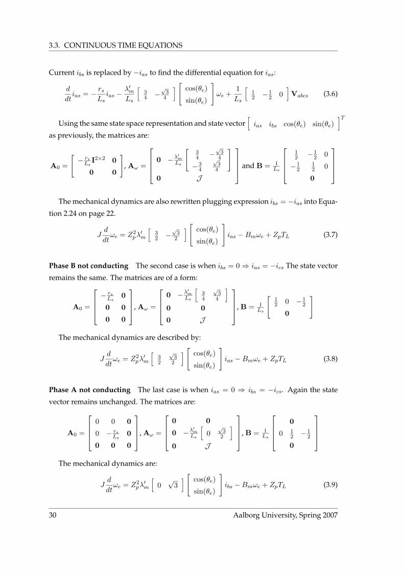
Group 1032c 29
3.3. CONTINUOUS TIME EQUATIONS
Current ibs is replaced by −ias to find the differential equation for ias:
d
dtias = − rs
Lsias −
λ′mLs
[34 −
√3
4
] [ cos(θe)
sin(θe)
]ωe +
1Ls
[12 −1
2 0]Vabcs (3.6)
Using the same state space representation and state vector[ias ibs cos(θe) sin(θe)
]Tas previously, the matrices are:
A0 =
[− rs
LsI2×2 0
0 0
], Aω =
0 −λ′mLs
[34 −
√3
4
−34
√3
4
]0 J
and B = 1Ls
12 −1
2 0
−12
12 0
0
The mechanical dynamics are also rewritten plugging expression ibs = −ias into Equa-
tion 2.24 on page 22.
Jd
dtωe = Z2
pλ′m
[32 −
√3
2
] [ cos(θe)
sin(θe)
]ias −Bmωe + ZpTL (3.7)
Phase B not conducting The second case is when ibs = 0 ⇒ ias = −ics The state vector
remains the same. The matrices are of a form:
A0 =
− rs
Ls0
0 0
0 0
, Aω =
0 −λ′m
Ls
[34
√3
4
]0 0
0 J
, B = 1Ls
[12 0 −1
2
0
]
The mechanical dynamics are described by:
Jd
dtωe = Z2
pλ′m
[32
√3
2
] [ cos(θe)
sin(θe)
]ias −Bmωe + ZpTL (3.8)
Phase A not conducting The last case is when ias = 0 ⇒ ibs = −ics. Again the state
vector remains unchanged. The matrices are:
A0 =
0 0 0
0 − rsLs
0
0 0 0
, Aω =
0 0
0 −λ′mLs
[0
√3
2
]0 J
, B = 1Ls
0
0 12 −1
2
0
The mechanical dynamics are:
Jd
dtωe = Z2
pλ′m
[0
√3] [ cos(θe)
sin(θe)
]ibs −Bmωe + ZpTL (3.9)
30 Aalborg University, Spring 2007
CHAPTER 3. HYBRID MODEL
3.4 FORMAL DESCRIPTION OF THE MODEL
Having the hybrid automaton for the BLDCM and the state space description for each
of the states of this automata, it is possible to write the formal description of the hybrid
model using Definition 1 on page 23.
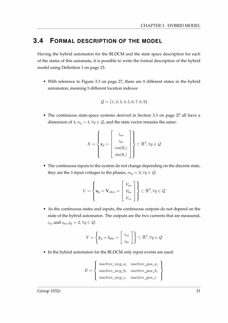
• With reference to Figure 3.3 on page 27, there are 9 different states in the hybrid
automaton, meaning 9 different location indexes:
Q = 1, 2, 3, 4, 5, 6, 7, 8, 9
• The continuous state-space systems derived in Section 3.3 on page 27 all have a
dimension of 4, nq = 4,∀q ∈ Q, and the state vector remains the same:
X =
xq =
ias
ibs
cos(θe)
sin(θe)
⊂ R4,∀q ∈ Q
• The continuous inputs to the system do not change depending on the discrete state,
they are the 3 input voltages to the phases, mq = 3,∀q ∈ Q:
U =
uq = Vabcs =
Vas
Vbs
Vcs
⊂ R3,∀q ∈ Q
• As the continuous states and inputs, the continuous outputs do not depend on the
state of the hybrid automaton. The outputs are the two currents that are measured,
ias and ibs, pq = 2,∀q ∈ Q:
Y =
yq = iabs =
[ias
ibs
]⊂ R2,∀q ∈ Q
• In the hybrid automaton for the BLDCM only input events are used:
E =
nactive_neg_a, nactive_pos_a,
nactive_neg_b, nactive_pos_b,
nactive_neg_c, nactive_pos_c
Group 1032c 31
3.4. FORMAL DESCRIPTION OF THE MODEL
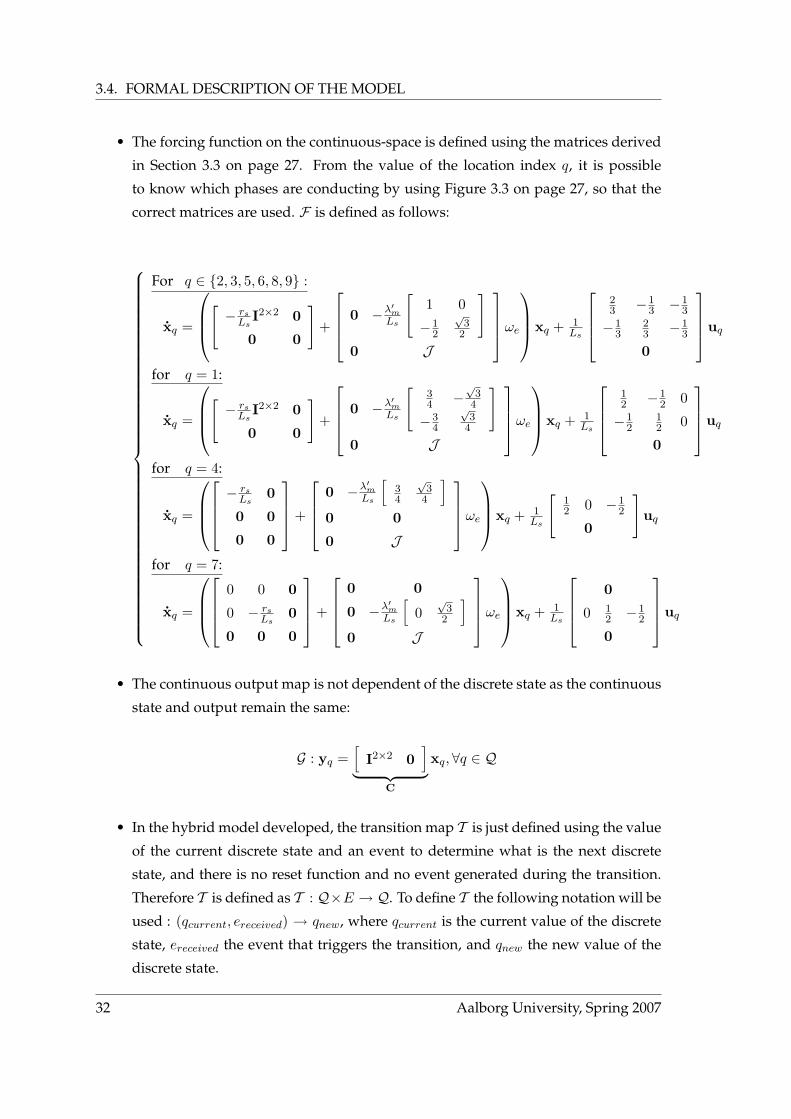
• The forcing function on the continuous-space is defined using the matrices derived
in Section 3.3 on page 27. From the value of the location index q, it is possible
to know which phases are conducting by using Figure 3.3 on page 27, so that the
correct matrices are used. F is defined as follows:
For q ∈ 2, 3, 5, 6, 8, 9 :
xq =
[− rs
LsI2×2 0
0 0
]+
0 −λ′mLs
[1 0
−12
√3
2
]0 J
ωe
xq + 1Ls
23 −1
3 −13
−13
23 −1
3
0
uq
for q = 1:
xq =
[− rs
LsI2×2 0
0 0
]+
0 −λ′mLs
[34 −
√3
4
−34
√3
4
]0 J
ωe
xq + 1Ls
12 −1
2 0
−12
12 0
0
uq
for q = 4:
xq =
− rs
Ls0
0 0
0 0
+
0 −λ′m
Ls
[34
√3
4
]0 0
0 J
ωe
xq + 1Ls
[12 0 −1
2
0
]uq
for q = 7:
xq =
0 0 0
0 − rsLs
0
0 0 0
+
0 0
0 −λ′mLs
[0
√3
2
]0 J
ωe
xq + 1Ls
0
0 12 −1
2
0
uq
• The continuous output map is not dependent of the discrete state as the continuous
state and output remain the same:
G : yq =[
I2×2 0]
︸ ︷︷ ︸C
xq,∀q ∈ Q
• In the hybrid model developed, the transition map T is just defined using the value
of the current discrete state and an event to determine what is the next discrete
state, and there is no reset function and no event generated during the transition.
Therefore T is defined as T : Q×E → Q. To define T the following notation will be
used : (qcurrent, ereceived) → qnew, where qcurrent is the current value of the discrete
state, ereceived the event that triggers the transition, and qnew the new value of the
discrete state.
32 Aalborg University, Spring 2007

CHAPTER 3. HYBRID MODEL
T :
(1, nactive_neg_b) → 2
(1, nactive_pos_b) → 3
(2, nactive_pos_b) → 4
(2, nactive_pos_a) → 6
(3, nactive_neg_b) → 4
(3, nactive_neg_a) → 5
(4, nactive_neg_a) → 5
(4, nactive_pos_a) → 6
(5, nactive_pos_a) → 7
(5, nactive_pos_c) → 9
(6, nactive_neg_a) → 7
(6, nactive_neg_c) → 8
(7, nactive_pos_c) → 9
(7, nactive_neg_c) → 8
(8, nactive_pos_c) → 1
(8, nactive_pos_b) → 3
(9, nactive_neg_c) → 1
(9, nactive_neg_b) → 2
3.5 TEST OF THE HYBRID MODEL
The hybrid model presented in the previous sections was implemented and tested in
[NP06]. The parameters of the motor used for the test were estimated and are given in
the following table:
Parameter Zp rs Ls λ′m J Bm
Value 3 3.8 [Ω] 0.0135 [H] 0.2225 [ Vrad·s−1 ] 0.002 [kg · m2] 5 · 10−4 [Kg · m2 · s−1]
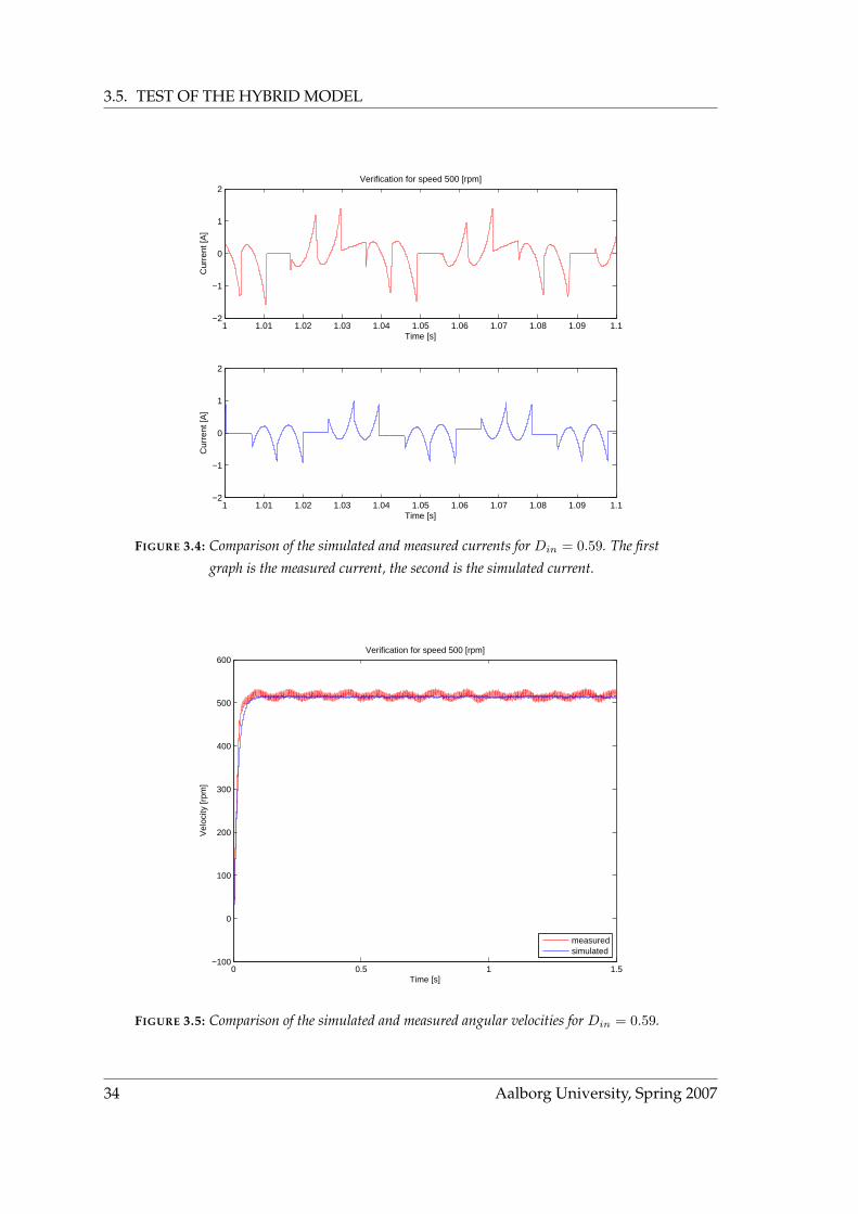
Simulations of the hybrid model were made, and the results were compared with mea-
surements taken on the real BLDCM with the same input duty cycle Din. Comparisons
were made for different values for Din, but only the results for Din = 0.59 are shown
as the same comments can be made for all different comparisons. Figure 3.4 on the fol-
lowing page is the comparison of the real and simulated currents of the BLDCM, and
Figure 3.5 on the next page is the comparison of the speed. The model has been studied
in [NP06] and has shown that the behaviour of the model is close to the real BLDCM.
Group 1032c 33
3.5. TEST OF THE HYBRID MODEL
1 1.01 1.02 1.03 1.04 1.05 1.06 1.07 1.08 1.09 1.1−2
−1
0
1
2Verification for speed 500 [rpm]
Cur
rent
[A]
Time [s]
1 1.01 1.02 1.03 1.04 1.05 1.06 1.07 1.08 1.09 1.1−2
−1
0
1
2
Cur
rent
[A]
Time [s]
FIGURE 3.4: Comparison of the simulated and measured currents for Din = 0.59. The first
graph is the measured current, the second is the simulated current.
0 0.5 1 1.5−100
0
100
200
300
400
500
600Verification for speed 500 [rpm]
Time [s]
Vel
ocity
[rpm
]
measuredsimulated
FIGURE 3.5: Comparison of the simulated and measured angular velocities for Din = 0.59.
34 Aalborg University, Spring 2007

CHAPTER 3. HYBRID MODEL
3.6 CONCLUSION
In this chapter the hybrid model of the BLDCM has been presented. A construction
of the hybrid automaton was shown followed by continuous equations and the formal
description of the whole system. Some of the results from the verification of the model
has been demonstrated to show that the model is sufficiently close to the real system.
Group 1032c 35

This page is left intentionally blank

4HYBRID OBSERVER
In this chapter, the new hybrid observer used to estimate the angle and the speed of the
rotor is presented. This observer is built based on the observer designed in [NP06]. The
core of the observer, i.e. the speed adaptive state estimation will be kept identical as it has
shown good capability to estimate the states. However, the structure of the observer is
modified. This is done in order to reduce the complexity of the observer and to improve
the precision of the estimates.
Firstly, the location automaton is described based on the reduced hybrid automaton
that was build in Section 3.2 on page 24. The new structure of the observer is presented,
and the new equations for the observer are expressed. Finally, the results of a test of this
observer will be presented.
As mentioned earlier, it is assumed that the angular velocity of the rotor is in certain
range of values, ωr ∈ [500; 1000] [rpm], that is approximately ωe ∈ [156; 315] [rad/s]. This
can be assumed as the speed of the pump is generally not varying in the full range, but
operates in a certain region.
4.1 LOCATION AUTOMATON
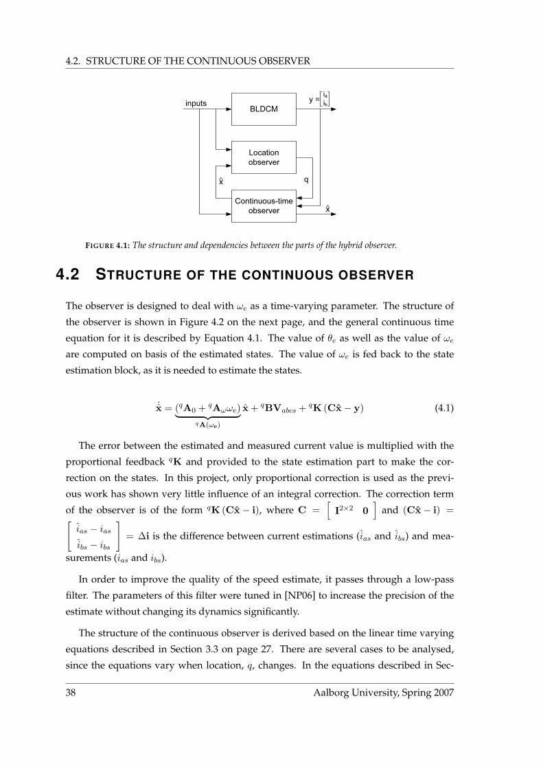
The hybrid observer consists of two parts: the location automaton and the continuous
observer. It is very similar to the definition of the hybrid system, which also consists of
those parts and the interactions between them.
Hybrid automaton was proposed in Section 3.2 on page 24, in accordance with certain
assumptions that are important based on the scope of the project. It includes the physical
behaviour of such a system and the control strategy.
The idea of the location observer is to track the current location of the system and give
this knowledge to the continuous part so that the proper set of equations can be chosen.
As shown in Figure 4.1 on the following page, the location observer switches based on
the estimated states from the continuous part. This prevents erroneous switching based
on noisy measurements and is important for the stability of the observer. In the system
that is analysed, the exact switching sequence is known. The initial state is also known
as there is the startup procedure that aligns the rotor to a known phase. Therefore the
location observer is simply a copy of the hybrid automaton.
Group 1032c 37
4.2. STRUCTURE OF THE CONTINUOUS OBSERVER
Locationobserver
Continuous-timeobserver
x
inputs
q
BLDCM
x
y = iaib
FIGURE 4.1: The structure and dependencies between the parts of the hybrid observer.
4.2 STRUCTURE OF THE CONTINUOUS OBSERVER
The observer is designed to deal with ωe as a time-varying parameter. The structure of
the observer is shown in Figure 4.2 on the next page, and the general continuous time
equation for it is described by Equation 4.1. The value of θe as well as the value of ωe
are computed on basis of the estimated states. The value of ωe is fed back to the state
estimation block, as it is needed to estimate the states.
˙x = (qA0 + qAωωe)︸ ︷︷ ︸qA(ωe)
x + qBVabcs + qK (Cx− y) (4.1)
The error between the estimated and measured current value is multiplied with the
proportional feedback qK and provided to the state estimation part to make the cor-
rection on the states. In this project, only proportional correction is used as the previ-
ous work has shown very little influence of an integral correction. The correction term
of the observer is of the form qK (Cx− i), where C =[
I2×2 0]
and (Cx− i) =[ias − ias
ibs − ibs
]= ∆i is the difference between current estimations (ias and ibs) and mea-
surements (ias and ibs).
In order to improve the quality of the speed estimate, it passes through a low-pass
filter. The parameters of this filter were tuned in [NP06] to increase the precision of the
estimate without changing its dynamics significantly.
The structure of the continuous observer is derived based on the linear time varying
equations described in Section 3.3 on page 27. There are several cases to be analysed,
since the equations vary when location, q, changes. In the equations described in Sec-
38 Aalborg University, Spring 2007

CHAPTER 4. HYBRID OBSERVER
BLDCM Currentsensors + +–
qK
∫qB
qA
C+++
+
u
x
∆i
Calculateangle and speed
θω
ias, ibs
ias, ibs
x
Filterωfilt
FIGURE 4.2: Block diagram of the observer structure at a location q.
tion 3.3 on page 27, the differential equations of the measurable states ias and ibs are
dependent on the time varying parameter ωe, which makes it difficult to design an adap-
tive observer. The idea is therefore to realize a state transformation in order to decouple
ωe from the measurable states. The new state vector, x, contains the two measurable
states ias and ibs, as well as two new states eα and eβ that are related to the back-EMF.
This approach was first presented in [UZ04]. In this work it is extended to fit a different
model description. The new parameters are defined as follows:
eα = ωe cos θe
eβ = ωe sin θe
(4.2)
The derivatives are then of a form:
eα = ωe cos θe − ω2e sin θe = eα
1ωeωe − eβωe
eβ = ωe sin θe + ω2e cos θe = eβ
1ωeωe + eαωe
(4.3)
The previous equation shows that the acceleration of the rotor ωe has an influence
on the dynamics, but since ωe is a time-varying parameter, it will be assumed in this
project that it is varying slowly compared to the other states, i.e. its derivative is zero,
ωe = 0. The acceleration of the rotor was used in the previous work, but it found to
Group 1032c 39

4.3. CALCULATION OF THE ANGLE AND THE SPEED
have little influence on the dynamics of the observer (when set to zero there are almost
no changes in the estimates), which explains why this assumption can be made. Under
this assumption, the derivatives become:
eα = −eβωe
eβ = eαωe
(4.4)
The observer equations may be derived and described for each of the locations, q,
where the state vector is of a form Equation 4.5.
x =[ias ibs eα eβ
]T(4.5)
4.3 CALCULATION OF THE ANGLE AND THE SPEED
The states eα and eβ depend only on the value of the angle and the speed, therefore the
estimations of the angle and angular velocity are computed on basis of those states.
The estimation of the angular velocity ωe is computed using Equation 4.6. This Equa-
tion is derived from the expression of eα and eβ in Equations 4.2 on the preceding page.
Since only one direction of the rotation is considered, ωe > 0, the absolute value can be
omitted.
ωe = |ωe| =√e2α + e2β (4.6)
The estimation of the angle of the rotor θe is also computed on basis of the estimated
states eα and eβ . First, cos θe and sin θe are calculated using Equation 4.7, which is derived
from Equations 4.2 on the preceding page.
cos θe =eαωe
sin θe =eβωe
(4.7)
From the values of sin θe and cos θe, the estimation of the angle is found as follows:
40 Aalborg University, Spring 2007
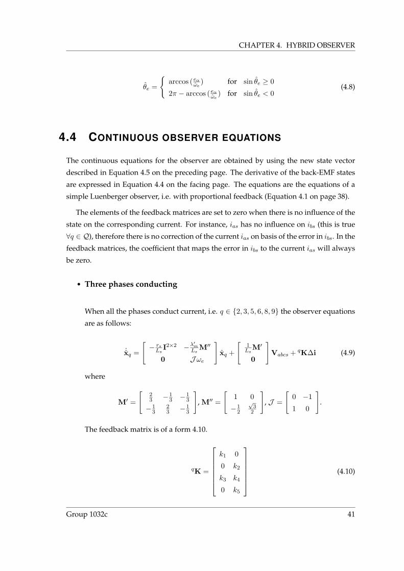
CHAPTER 4. HYBRID OBSERVER
θe =
arccos ( eα
ωe) for sin θe ≥ 0
2π − arccos ( eαωe
) for sin θe < 0(4.8)
4.4 CONTINUOUS OBSERVER EQUATIONS
The continuous equations for the observer are obtained by using the new state vector
described in Equation 4.5 on the preceding page. The derivative of the back-EMF states
are expressed in Equation 4.4 on the facing page. The equations are the equations of a
simple Luenberger observer, i.e. with proportional feedback (Equation 4.1 on page 38).
The elements of the feedback matrices are set to zero when there is no influence of the
state on the corresponding current. For instance, ias has no influence on ibs (this is true
∀q ∈ Q), therefore there is no correction of the current ias on basis of the error in ibs. In the
feedback matrices, the coefficient that maps the error in ibs to the current ias will always
be zero.
• Three phases conducting
When all the phases conduct current, i.e. q ∈ 2, 3, 5, 6, 8, 9 the observer equations
are as follows:
˙xq =
[− rs
LsI2×2 −λ′m
LsM′′
0 Jωe
]xq +
[1
LsM′
0
]Vabcs + qK∆i (4.9)
where
M′ =
[23 −1
3 −13
−13
23 −1
3
], M′′ =
[1 0
−12
√3
2
], J =
[0 −1
1 0
].
The feedback matrix is of a form 4.10.
qK =
k1 0
0 k2
k3 k4
0 k5
(4.10)
Group 1032c 41

4.4. CONTINUOUS OBSERVER EQUATIONS
• C phase passive
When phase C is passive, i.e. q = 1, the observer’s equations are as follows:
˙x1 =
[− rs
LsI2×2 −λ′m
Ls
1M′′
0 Jωe
]x1 +
[1
Ls
1M′
0
]Vabcs + 1K∆i (4.11)
where
1M′ =
[12 −1
2 0
−12
12 0
], 1M′′ =
[34 −
√3
4
−34
√3
4
].
The feedback matrix is of a form 4.12.
1K =
k6 0
0 k7
k8 0
k9 0
(4.12)
• B phase passive
When phase B is passive, i.e. q = 4, the observer’s equations are as follows:
˙x4 =
[− rs
Ls0
0 0
]−λ′m
Ls
4M′′
0 Jωe
x4 +
[1
Ls
4M′
0
]Vabcs + 4K∆i (4.13)
where
4M′ =
[12 0 −1
2
0 0 0
], 4M′′ =
[34
√3
4
0 0
].
The feedback matrix is of a form 4.14.
4K =
k10 0
0 0
k11 0
k12 0
(4.14)
42 Aalborg University, Spring 2007
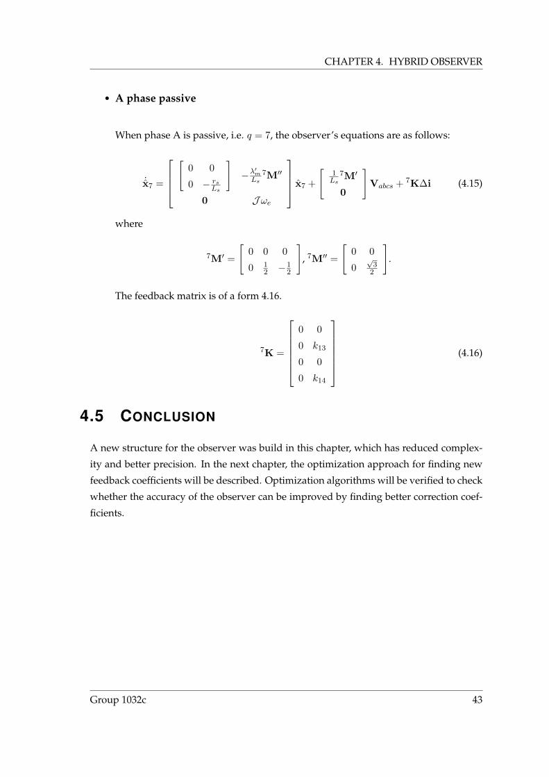
CHAPTER 4. HYBRID OBSERVER
• A phase passive
When phase A is passive, i.e. q = 7, the observer’s equations are as follows:
˙x7 =
[
0 0
0 − rsLs
]−λ′m
Ls
7M′′
0 Jωe
x7 +
[1
Ls
7M′
0
]Vabcs + 7K∆i (4.15)
where
7M′ =
[0 0 0
0 12 −1
2
], 7M′′ =
[0 0
0√
32
].
The feedback matrix is of a form 4.16.
7K =
0 0
0 k13
0 0
0 k14
(4.16)
4.5 CONCLUSION
A new structure for the observer was build in this chapter, which has reduced complex-
ity and better precision. In the next chapter, the optimization approach for finding new
feedback coefficients will be described. Optimization algorithms will be verified to check
whether the accuracy of the observer can be improved by finding better correction coef-
ficients.
Group 1032c 43

This page is left intentionally blank

5OPTIMIZATION OFOBSERVER FEEDBACK
The core part of the design of the observer is the optimization of the feedback parameters,
as it is very difficult if not impossible to explicitly find the coefficients subject to the
constraints imposed in the previous chapters. This chapter describes the problem of the
feedback design from an optimization point of view. It gives an overview of some of the
existing methods that could be applied to this problem. The most suitable methods are
then implemented, and applied to the problem.
5.1 PROBLEM OVERVIEW
The problem of the observer design lies in finding correct values of the feedback matricesqK, such that the error of estimation converges to zero. In order to achieve this, a cost
function is introduced. The cost function Q is defined as follows1:
Q =∣∣∣∣∫ t+τ
teθ(t)dt
∣∣∣∣︸ ︷︷ ︸Mean
+∫ t+τ
te2θ(t)dt︸ ︷︷ ︸
V ariance
(5.1)
The value eθ(t) is a difference between the electrical angle estimated by the observer,
θe, and the measured electrical angle, θe. [t; t + τ ] is the time range for which the cost
function is calculated. The choice of the value of τ is a trade-off between the time of
computation of the cost function and the quantity of information included in the cost
function, in this project τ will be 0.5 [s]. The cost function will be calculated on a set of
data corresponding to a step in the angular velocity from 0 to 500 [rpm], which means that
the coefficients will be optimized for this speed. A step in the angular velocity is chosen
as it allows to optimize the convergence time of the observer as well as its steady state
performance.
The cost function described by Equation 5.1 was chosen so that it represents the sum
of the variance (when mean is zero) and the absolute value of the mean of the estimation
error. Those are the two values to be minimized in order to have a good estimation of the
1It can be noticed in Equation 5.1 that the mean value is already included in the term that represents the
variance (which explains why this term represents the variance only when the mean is zero). However, from
the practical point of view, the cost function of this type has shown to be more efficient than the cost function
without mean value term.
Group 1032c 45
5.2. RANDOM SEARCH METHODS
angle of the rotor.
Optimization limitations
There are a several key assumptions and important features of the problem, that should
be taken into consideration before choosing a suitable optimization strategy. The opti-
mization is run off-line, based on measurements taken from a real system. It requires
input signals to the system and corresponding measurements of the currents, rotor angle
and velocity. The goal is to tune the feedback parameters so that the observer follows the
hybrid trajectory of the real system as closely as it is possible.
Overall there are 14 feedback parameters k in the matrices qK that need to be deter-
mined. Due to the system complexity it is very difficult if not impossible to calculate the
gradient of the performance function with respect to the feedback gains. The problem is
highly non-linear and multidimensional. The optimization is done through very compu-
tational demanding simulations. Because of this, the number of potential methods that
could be applied is limited.
The results of an optimized observer trajectory must be compared to the real system.
This however implies that for each set of values k, the system must be simulated and its
output must be stored for comparison purposes. The problem lies in the duration and
complexity of the simulation of such a system, while using Simulink R© software. It takes
several seconds, to simulate 0.5 [s] of the system’s performance, i.e. the cost function. The
cost function must be evaluated many times, thus it is important to minimize the compu-
tational demands of the system, by writing an efficient code. This problem is deliberated
in Appendix B on page 105, where unnecessary computations in the previously establi-
shed model are removed. Nonetheless, the time of computation of one iteration plays a
key role when choosing the optimization strategy.
Due to the complexity of the problem and other limitations, conventional optimization
techniques cannot be used in the optimization problem of finding feedback coefficients
for the non-linear hybrid observer. Other techniques must be adapted to this problem.
5.2 RANDOM SEARCH METHODS
Random Weight Change (RWC) algorithm is an example of a random search algorithm
that can be used in Artificial Neural Networks (ANN) training. It is a probabilistic
46 Aalborg University, Spring 2007
CHAPTER 5. OPTIMIZATION OF OBSERVER FEEDBACK
method that is opposed to deterministic methods like backpropagation. During each
of the cycles, the set of parameters is perturbed randomly with a magnitude δ. The cost
is calculated and compared with the cost using previous set of parameters. If the value is
smaller, then the new set of parameters replaces the previous values. One of the biggest
advantages of such an approach is the simplicity of this algorithm. It can be easily imple-
mented and more importantly it is fast [KHB+98].
In the previous work [NP06], RWC has shown good performance for finding an op-
timization region. Acquiring very precise values was not a goal for this algorithm, the
goal was rather to find a good initial point for another optimization strategy.
5.3 PARTICLE SWARM OPTIMIZATION
Particle Swarm Optimization (PSO) belongs to a new research area of Swarm Intelligence
(SI). It bases its strategy on the analogy to a swarm of birds or school of fish. The popu-
lation, called swarm, is a potential set of solutions. It then tries to iteratively explore the
whole search area in analogy to a search for food. During this process, the particles, that
is the individuals of the swarm, exchange the informations among each other. All the
particles benefit from this strategy [WQ05].
According to [WQ05], PSO exhibits good performance in solving hard optimization prob-
lems and engineering applications, and compares favourably to other optimization algorithms.
Nonlinear Simplex Search (NSS) is a Hybrid PSO algorithm, that has shown some advan-
tages over other optimization techniques, like Evolutionary Algorithms or Tabu Search
[WQ05].
In the case of the optimization of k parameters, NSS was used for fine tuning the
values in [NP06]. The initial point for this algorithm was determined by RWC.
5.4 EVOLUTIONARY COMPUTATION
This class of algorithms uses Darwinian evolution theory as a method for determining
an optimum point. It is inspired by mechanisms found in nature, namely selection and
adaptation. The problems dealt with by such computational systems are usually highly non-
linear and contain inaccurate and noisy data [SMY03, p. 27]. This is exactly the case with the
observer optimization.
Group 1032c 47
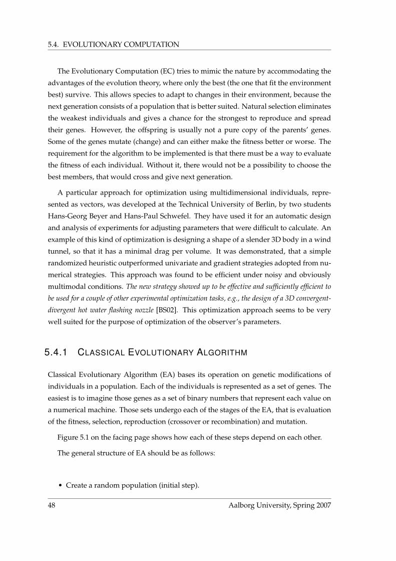
5.4. EVOLUTIONARY COMPUTATION
The Evolutionary Computation (EC) tries to mimic the nature by accommodating the
advantages of the evolution theory, where only the best (the one that fit the environment
best) survive. This allows species to adapt to changes in their environment, because the
next generation consists of a population that is better suited. Natural selection eliminates
the weakest individuals and gives a chance for the strongest to reproduce and spread
their genes. However, the offspring is usually not a pure copy of the parents’ genes.
Some of the genes mutate (change) and can either make the fitness better or worse. The
requirement for the algorithm to be implemented is that there must be a way to evaluate
the fitness of each individual. Without it, there would not be a possibility to choose the
best members, that would cross and give next generation.
A particular approach for optimization using multidimensional individuals, repre-
sented as vectors, was developed at the Technical University of Berlin, by two students
Hans-Georg Beyer and Hans-Paul Schwefel. They have used it for an automatic design
and analysis of experiments for adjusting parameters that were difficult to calculate. An
example of this kind of optimization is designing a shape of a slender 3D body in a wind
tunnel, so that it has a minimal drag per volume. It was demonstrated, that a simple
randomized heuristic outperformed univariate and gradient strategies adopted from nu-
merical strategies. This approach was found to be efficient under noisy and obviously
multimodal conditions. The new strategy showed up to be effective and sufficiently efficient to
be used for a couple of other experimental optimization tasks, e.g., the design of a 3D convergent-
divergent hot water flashing nozzle [BS02]. This optimization approach seems to be very
well suited for the purpose of optimization of the observer’s parameters.
5.4.1 CLASSICAL EVOLUTIONARY ALGORITHM
Classical Evolutionary Algorithm (EA) bases its operation on genetic modifications of
individuals in a population. Each of the individuals is represented as a set of genes. The
easiest is to imagine those genes as a set of binary numbers that represent each value on
a numerical machine. Those sets undergo each of the stages of the EA, that is evaluation
of the fitness, selection, reproduction (crossover or recombination) and mutation.
Figure 5.1 on the facing page shows how each of these steps depend on each other.
The general structure of EA should be as follows:
• Create a random population (initial step).
48 Aalborg University, Spring 2007
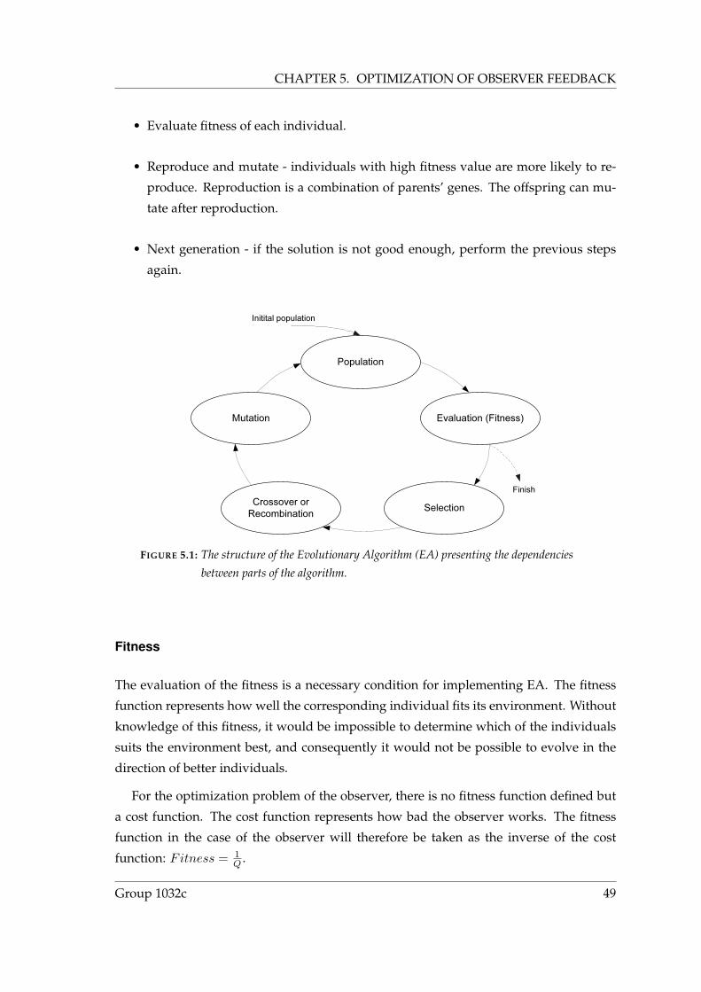
CHAPTER 5. OPTIMIZATION OF OBSERVER FEEDBACK
• Evaluate fitness of each individual.
• Reproduce and mutate - individuals with high fitness value are more likely to re-
produce. Reproduction is a combination of parents’ genes. The offspring can mu-
tate after reproduction.
• Next generation - if the solution is not good enough, perform the previous steps
again.
SelectionCrossover or Recombination
Evaluation (Fitness)
Population
Initital population
Finish
Mutation
FIGURE 5.1: The structure of the Evolutionary Algorithm (EA) presenting the dependencies
between parts of the algorithm.
Fitness
The evaluation of the fitness is a necessary condition for implementing EA. The fitness
function represents how well the corresponding individual fits its environment. Without
knowledge of this fitness, it would be impossible to determine which of the individuals
suits the environment best, and consequently it would not be possible to evolve in the
direction of better individuals.
For the optimization problem of the observer, there is no fitness function defined but
a cost function. The cost function represents how bad the observer works. The fitness
function in the case of the observer will therefore be taken as the inverse of the cost
function: Fitness = 1Q .
Group 1032c 49
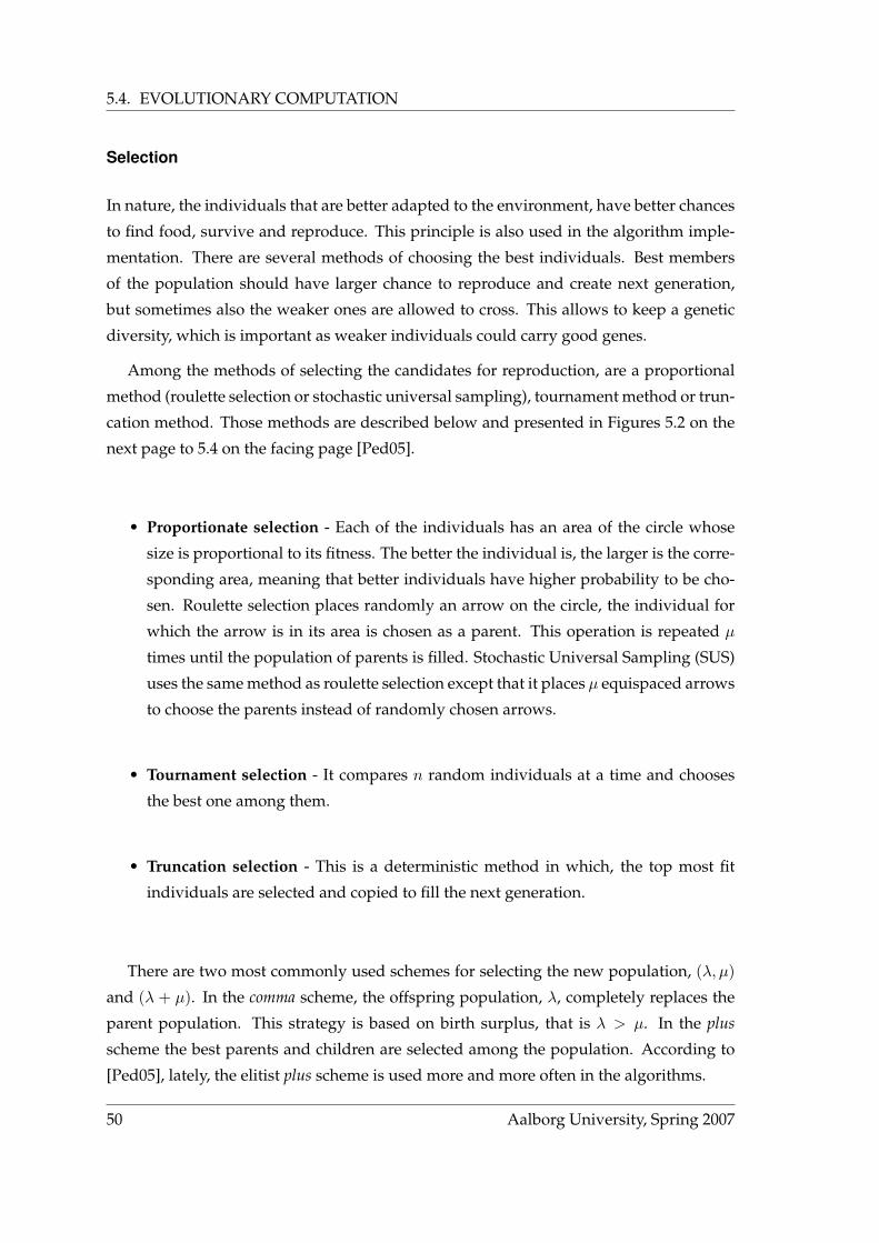
5.4. EVOLUTIONARY COMPUTATION
Selection
In nature, the individuals that are better adapted to the environment, have better chances
to find food, survive and reproduce. This principle is also used in the algorithm imple-
mentation. There are several methods of choosing the best individuals. Best members
of the population should have larger chance to reproduce and create next generation,
but sometimes also the weaker ones are allowed to cross. This allows to keep a genetic
diversity, which is important as weaker individuals could carry good genes.
Among the methods of selecting the candidates for reproduction, are a proportional
method (roulette selection or stochastic universal sampling), tournament method or trun-
cation method. Those methods are described below and presented in Figures 5.2 on the
next page to 5.4 on the facing page [Ped05].
• Proportionate selection - Each of the individuals has an area of the circle whose
size is proportional to its fitness. The better the individual is, the larger is the corre-
sponding area, meaning that better individuals have higher probability to be cho-
sen. Roulette selection places randomly an arrow on the circle, the individual for
which the arrow is in its area is chosen as a parent. This operation is repeated µ
times until the population of parents is filled. Stochastic Universal Sampling (SUS)
uses the same method as roulette selection except that it places µ equispaced arrows
to choose the parents instead of randomly chosen arrows.
• Tournament selection - It compares n random individuals at a time and chooses
the best one among them.
• Truncation selection - This is a deterministic method in which, the top most fit
individuals are selected and copied to fill the next generation.
There are two most commonly used schemes for selecting the new population, (λ, µ)
and (λ + µ). In the comma scheme, the offspring population, λ, completely replaces the
parent population. This strategy is based on birth surplus, that is λ > µ. In the plus
scheme the best parents and children are selected among the population. According to
[Ped05], lately, the elitist plus scheme is used more and more often in the algorithms.
50 Aalborg University, Spring 2007
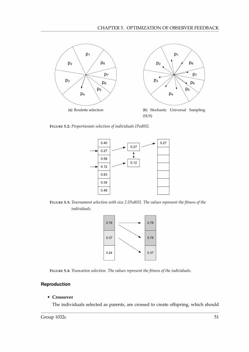
CHAPTER 5. OPTIMIZATION OF OBSERVER FEEDBACK
8
1
2
3
45
6
7
(a) Roulette selection
8
1
2
3
45
6
7
(b) Stochastic Universal Sampling
(SUS)
FIGURE 5.2: Proportionate selection of individuals [Ped05].
0.40
0.27
0.58
0.12
0.83
0.34
0.48
0.12
0.270.27
FIGURE 5.3: Tournament selection with size 2 [Ped05]. The values represent the fitness of the
individuals.
0.24
0.780.78
0.37
0.37
0.78
FIGURE 5.4: Truncation selection. The values represent the fitness of the individuals.
Reproduction
• Crossover
The individuals selected as parents, are crossed to create offspring, which should
Group 1032c 51

5.4. EVOLUTIONARY COMPUTATION
hopefully improve the fitness of the population.
Crossover is a genetic operator that is inspired by the reproduction of the highest
species in the nature. This operator can be implemented in several ways.
The simplest and most common is the single point crossover. Having two binary
strings, that represent two real number, a random point in the string is chosen. The
strings are then swapped. This is illustrated in Figure 5.5. Similarly, there might
also be n-point crossover which is also illustrated in the same figure. This operator
can be considered as random shuffle.
There also exist methods for using real valued numbers in crossing. There are
two widely used methods to do so, blended crossover (BLX) and simulated binary
crossover (SBX). Those methods are not further discussed as they are not further
used. To find more details about them, please refer to [Ped05].
(a) Single point (b) Triple point
FIGURE 5.5: Example of a crossover for a binary string [Ped05].
• Recombination
There exist many widely used methods for the recombination. Among the most
common is an intermediate recombination. The procedure is done according to the
formula:
xoi = α · xp1
i + (1− α) · xp2i
where x is the set of optimization parameters, α is randomly chosen parameter from
a uniform distribution with interval [0, 1], superscript o corresponds to offspring and
p corresponds to parent. When α = 0.5, the value of offspring is simply the mean
value of its parents. This is illustrated in Figure 5.6 on the facing page.
52 Aalborg University, Spring 2007
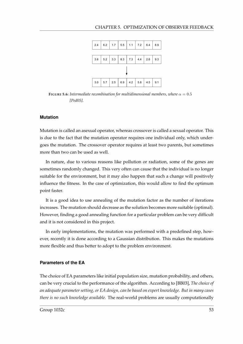
CHAPTER 5. OPTIMIZATION OF OBSERVER FEEDBACK
2.4 6.2
3.6 5.2 3.3 8.3 7.3 4.4 2.6 9.3
1.7 5.5 1.1 7.2 6.4 8.9
3.0 5.7 2.5 6.9 4.2 5.8 4.5 9.1
FIGURE 5.6: Intermediate recombination for multidimensional members, where α = 0.5
[Ped05].
Mutation
Mutation is called an asexual operator, whereas crossover is called a sexual operator. This
is due to the fact that the mutation operator requires one individual only, which under-
goes the mutation. The crossover operator requires at least two parents, but sometimes
more than two can be used as well.
In nature, due to various reasons like pollution or radiation, some of the genes are
sometimes randomly changed. This very often can cause that the individual is no longer
suitable for the environment, but it may also happen that such a change will positively
influence the fitness. In the case of optimization, this would allow to find the optimum
point faster.
It is a good idea to use annealing of the mutation factor as the number of iterations
increases. The mutation should decrease as the solution becomes more suitable (optimal).
However, finding a good annealing function for a particular problem can be very difficult
and it is not considered in this project.
In early implementations, the mutation was performed with a predefined step, how-
ever, recently it is done according to a Gaussian distribution. This makes the mutations
more flexible and thus better to adopt to the problem environment.
Parameters of the EA
The choice of EA parameters like initial population size, mutation probability, and others,
can be very crucial to the performance of the algorithm. According to [BB03], The choice of
an adequate parameter setting, or EA design, can be based on expert knowledge. But in many cases
there is no such knowledge available. The real-world problems are usually computationally
Group 1032c 53

5.4. EVOLUTIONARY COMPUTATION
demanding, therefore it is important to have a good initial population. There is no explicit
way of finding the parameters, therefore there exist other methods to determine them.
An example could be design of experiment (DOE) techniques presented in [BB03]. There
are also techniques that allow self-tuning of such algorithms, in order to optimize the
algorithm parameters on-line, while it is executed [BS02].
The evolutionary techniques of optimization can be very sensitive to those internal
parameters. An evolutionary window is a term to describe the range of parameters for
which an EA performs well. If some of them are chosen wrongly, the algorithm will not
work.
5.4.2 DIFFERENTIAL EVOLUTION
Differential Evolution (DE) is an optimization algorithm which uses the idea of the gra-
dient algorithm, i.e. it uses differences in the value of the cost function of the individuals
to create better individuals. In the DE, the idea of the gradient algorithm is combined
with the classical EA [UV03]. This algorithm is of (λ + µ) type, which means that only
the best individuals are kept. The general structure of the DE is as follows:
1. Create a random population and evaluate fitness of each individual (initial step).
2. For each individual xpi in the population, create an offspring xo
i .
3. Evaluate the offspring xoi .
4. If xoi is better than the parent xp
i , copy it in the next population, otherwise copy xpi
in the next population.
5. Next generation - if the solution is not good enough, perform the previous steps
again with the new population.
The core part of this algorithm is the way of creating the offspring xoi . Several variants
for creating the new candidate have been proposed. The offspring is generally built by
first creating an intermediate offspring xoi ’.
• In [UV03], in order to create xoi ’, three extra parents of the current population xp1
i ,
xp2i , and xp3
i different from the current parent xpi are randomly chosen. Equation 5.2
on the next page represents how xoi ’ is built, with F being a scaling factor, and Q(x)
54 Aalborg University, Spring 2007
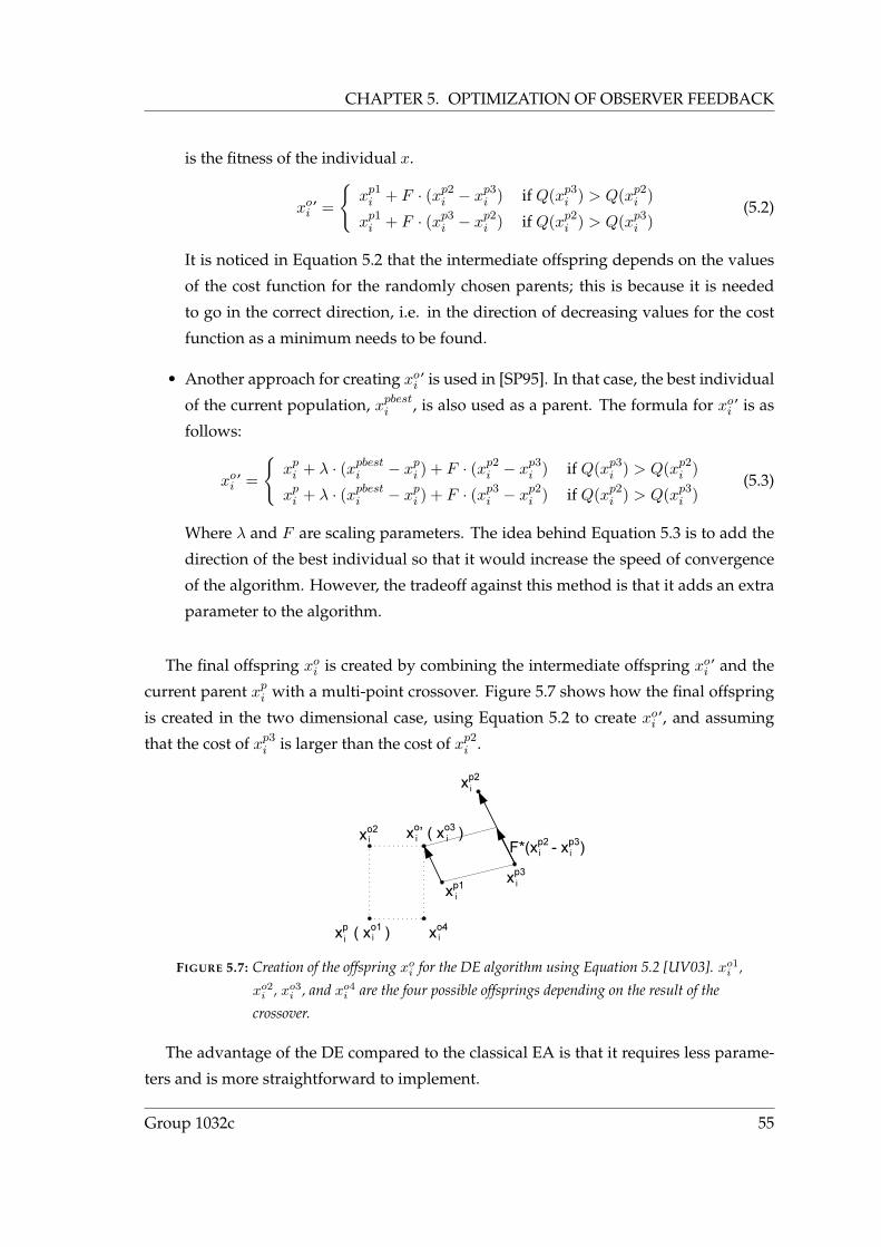
CHAPTER 5. OPTIMIZATION OF OBSERVER FEEDBACK
is the fitness of the individual x.
xoi ’ =
xp1
i + F · (xp2i − xp3
i ) if Q(xp3i ) > Q(xp2
i )
xp1i + F · (xp3
i − xp2i ) if Q(xp2
i ) > Q(xp3i )
(5.2)
It is noticed in Equation 5.2 that the intermediate offspring depends on the values
of the cost function for the randomly chosen parents; this is because it is needed
to go in the correct direction, i.e. in the direction of decreasing values for the cost
function as a minimum needs to be found.
• Another approach for creating xoi ’ is used in [SP95]. In that case, the best individual
of the current population, xpbesti , is also used as a parent. The formula for xo
i ’ is as
follows:
xoi ’ =
xp
i + λ · (xpbesti − xp
i ) + F · (xp2i − xp3
i ) if Q(xp3i ) > Q(xp2
i )
xpi + λ · (xpbest
i − xpi ) + F · (xp3
i − xp2i ) if Q(xp2
i ) > Q(xp3i )
(5.3)
Where λ and F are scaling parameters. The idea behind Equation 5.3 is to add the
direction of the best individual so that it would increase the speed of convergence
of the algorithm. However, the tradeoff against this method is that it adds an extra
parameter to the algorithm.
The final offspring xoi is created by combining the intermediate offspring xo
i ’ and the
current parent xpi with a multi-point crossover. Figure 5.7 shows how the final offspring
is created in the two dimensional case, using Equation 5.2 to create xoi ’, and assuming
that the cost of xp3i is larger than the cost of xp2
i .
xo’ ( xo3 )xo2
xp ( xo1 )
xp1
xp2
xp3
xo4
i i i
i
ii
iii
F*(xp2 - xp3)i i
FIGURE 5.7: Creation of the offspring xoi for the DE algorithm using Equation 5.2 [UV03]. xo1
i ,
xo2i , xo3
i , and xo4i are the four possible offsprings depending on the result of the
crossover.
The advantage of the DE compared to the classical EA is that it requires less parame-
ters and is more straightforward to implement.
Group 1032c 55

5.5. IMPLEMENTATION AND VERIFICATION
In the next section, the different optimization algorithms presented will be imple-
mented and applied to the problem. This study should allow to come up with a general
approach for finding the feedback parameters of the observer, so that the optimization
method could be re-used with an observer for a BLDCM with different electrical param-
eters.
5.5 IMPLEMENTATION AND VERIFICATION
This section describes the implementation of the most beneficial algorithms suitable for
the problem. The NSS algorithm was already used and tested previously in [NP06]. It
has shown rather good performance, however, new optimization approaches are verified
in order to choose the most suitable solution. Therefore implementation of NSS is not
described nor verified in this chapter.
The optimization of feedback gains is run off-line in MATLAB R©/Simulink R©.
RWC
A very important parameter for many optimization algorithms is an initial population or
a starting point. Very often the optimization is preceded by an analysis of the problem
that establishes a starting point. For the optimization of the observer’s feedback matrices
the RWC algorithm is used to find the starting point. This algorithm is very fast, as it
only requires one run of the simulation per epoch, which makes it suitable for scanning
the optimization area.
The algorithm’s flow chart is presented in Figure 5.8 on the facing page. The algo-
rithm, perturbs the optimization coefficients with a random variable δ with distribution
N (0, σ2). The perturbed coefficients are defined as follows (where j is the index of the
coefficient):
kperturbed,j = kprevious,j + δ ·√kprevious,j , 1 ≤ j ≤ 14
The advantage of this formula is that the variance of the perturbation adapts to the value
of the corresponding coefficient, the variance of the perturbation is σ2 · kprevious,j . When
the perturbed coefficients are more suitable than the previous coefficients, that is the cost
function is smaller, they are saved and the perturbation occurs from this point again.
The performance of a few random runs is depicted in Figure 5.9 on the next page. As
56 Aalborg University, Spring 2007
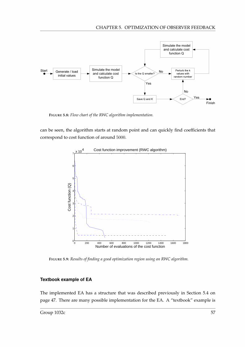
CHAPTER 5. OPTIMIZATION OF OBSERVER FEEDBACK
Generate / load initial values
Start Simulate the model and calculate cost
function QIs the Q smaller?
Perturb the k values with
random number
Simulate the model and calculate cost
function Q
End?Finish
No
YesNo
Save Q and K
Yes
FIGURE 5.8: Flow chart of the RWC algorithm implementation.
can be seen, the algorithm starts at random point and can quickly find coefficients that
correspond to cost function of around 5000.
0 200 400 600 800 1000 1200 1400 1600 18000
1
2
3
4
5
6
7 x 10
4 Cost function improvement (RWC algorithm)
Number of evaluations of the cost function
Cos
t fun
ctio
n (Q
)
FIGURE 5.9: Results of finding a good optimization region using an RWC algorithm.
Textbook example of EA
The implemented EA has a structure that was described previously in Section 5.4 on
page 47. There are many possible implementation for the EA. A “textbook” example is
Group 1032c 57
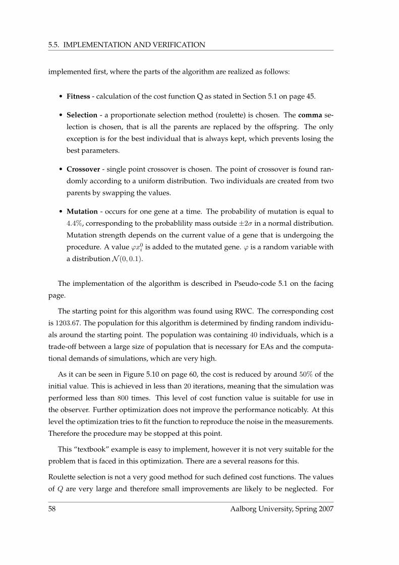
5.5. IMPLEMENTATION AND VERIFICATION
implemented first, where the parts of the algorithm are realized as follows:
• Fitness - calculation of the cost function Q as stated in Section 5.1 on page 45.
• Selection - a proportionate selection method (roulette) is chosen. The comma se-
lection is chosen, that is all the parents are replaced by the offspring. The only
exception is for the best individual that is always kept, which prevents losing the
best parameters.
• Crossover - single point crossover is chosen. The point of crossover is found ran-
domly according to a uniform distribution. Two individuals are created from two
parents by swapping the values.
• Mutation - occurs for one gene at a time. The probability of mutation is equal to
4.4%, corresponding to the probablility mass outside ±2σ in a normal distribution.
Mutation strength depends on the current value of a gene that is undergoing the
procedure. A value ϕx0i is added to the mutated gene. ϕ is a random variable with
a distribution N (0, 0.1).
The implementation of the algorithm is described in Pseudo-code 5.1 on the facing
page.
The starting point for this algorithm was found using RWC. The corresponding cost
is 1203.67. The population for this algorithm is determined by finding random individu-
als around the starting point. The population was containing 40 individuals, which is a
trade-off between a large size of population that is necessary for EAs and the computa-
tional demands of simulations, which are very high.
As it can be seen in Figure 5.10 on page 60, the cost is reduced by around 50% of the
initial value. This is achieved in less than 20 iterations, meaning that the simulation was
performed less than 800 times. This level of cost function value is suitable for use in
the observer. Further optimization does not improve the performance noticably. At this
level the optimization tries to fit the function to reproduce the noise in the measurements.
Therefore the procedure may be stopped at this point.
This “textbook” example is easy to implement, however it is not very suitable for the
problem that is faced in this optimization. There are a several reasons for this.
Roulette selection is not a very good method for such defined cost functions. The values
of Q are very large and therefore small improvements are likely to be neglected. For
58 Aalborg University, Spring 2007

CHAPTER 5. OPTIMIZATION OF OBSERVER FEEDBACK
N population size, n number of genes, xo offspring, xp parent, ψ ran-
dom variable N (0, 0.1).
Initialize the population with random individuals around the starting
point.
1. Simulate the observer with given set of feedback parameters and
calculate cost functions Q for all the individuals in the population
2. Calculate probabilities for each individual i to be chosen as a parent
Pi =1
Qi∑µi=1
1Qi
3. Choose N parents using roulette selection.
4. Generate random crossover point c and cross the parents according
to the formula (using Matlab-like notation)xo1
i =[xp1
i (1 : c) xp2i (c+ 1 : n)
]xo2
i =[xp2
i (1 : c) xp1i (c+ 1 : n)
]5. Mutate random elements.
For each offspring xoi
for each element j
if randn > mutation_threshold
xoi (j) = xo
i (j) + ψ ·√xo
i (j)
end for
end for
6. Replace the first offspring xo1 with the best individual from the pre-
vious population.
7. Replace previous population by offspring.
Next iteration
PSEUDO-CODE 5.1: Description of the “textbook” EA used in finding feedback coefficients.
example, if in a population consisting of three individuals, the cost values are Q1 = 5000,
Q2 = 5050 and Q3 = 5060, the probability of selecting the best individual is almost the
same as choosing the worst one.
Group 1032c 59

5.5. IMPLEMENTATION AND VERIFICATION
0 100 200 300 400 500 600 700 800600
700
800
900
1000
1100
1200
1300Cost function improvement ("textbook" EA algorithm)
Number of evaluations of the cost function
Cos
t fun
ctio
n (Q
)
FIGURE 5.10: Results of an optimization using “textbook” EA.
Single point crossover is not very well suited when some of the feedback coefficients are
related or dependent on each other. For example, when k1 and k14 are related and must
be changed in the same manner, single point crossover would not allow. Therefore a
multi-point crossover or recombination should be used to avoid this problem.
EA with tournament selection and recombination
A more suitable version of classical EA used for the optimization utilises tournament
selection and intermediate recombination methods. It is realized as follows:
• Fitness - calculation of the cost function Q as stated in Section 5.1 on page 45.
• Selection - a tournament method of selection is chosen, where 2 random individu-
als are compared at a time. The selection is performed according to comma strategy,
but the best individual is always kept.
• Recombination - intermediate recombination is chosen.
• Mutation - is realized the same way as in the “textbook” EA implementation, using
the same parameters.
60 Aalborg University, Spring 2007

CHAPTER 5. OPTIMIZATION OF OBSERVER FEEDBACK
The implementation of the EA with tournament selection and intermediate recombi-
nation is described in Pseudo-code 5.2. The starting point and the population size for this
algorithm were the same as previously in “textbook” EA.
N population size, xo offspring, xp parent, ψ random variableN (0, 0.1),
α random number with uniform distribution in [0; 1].
Initialize the population with random individuals around the starting
point.
1. Simulate the observer with given set of feedback parameters and
calculate cost functions Q for all the individuals in the population
2. SelectN parents using tournament selection comparing two individ-
uals at a time.
3. Find offspring using intermediate recombination, according to:
xoi = α · xp1
i + (1− α) · xp2i
4. Mutate random elements.
For each offspring xoi
for each element j
if randn > mutation_threshold
xoi (j) = xo
i (j) + ψ ·√xo
i (j)
end for
end for
5. Replace the first offspring xo1 with the best individual from the pre-
vious population.
6. Replace previous population by offspring.
Next iteration
PSEUDO-CODE 5.2: Description of the “improved” EA.
As it can be seen from Figure 5.11 on the following page, the number of iterations
to achieve a half of initial cost value is larger than in case of “textbook” EA. However,
this does not necessarily imply that this approach is worse than the previous one. The
performance of EAs depends significantly on the evolutionary window, but this is not
going to be investigated in this report.
Group 1032c 61
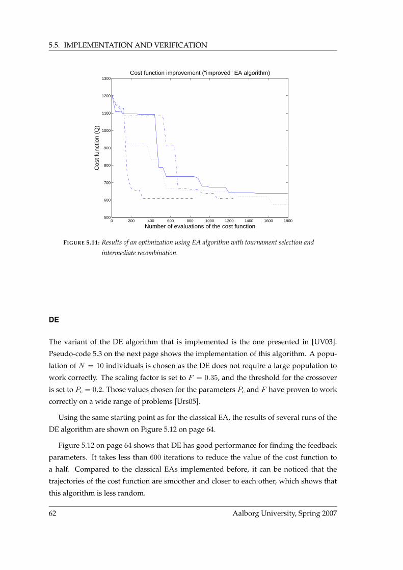
5.5. IMPLEMENTATION AND VERIFICATION
0 200 400 600 800 1000 1200 1400 1600 1800500
600
700
800
900
1000
1100
1200
1300Cost function improvement ("improved" EA algorithm)
Number of evaluations of the cost function
Cos
t fun
ctio
n (Q
)
FIGURE 5.11: Results of an optimization using EA algorithm with tournament selection and
intermediate recombination.
DE
The variant of the DE algorithm that is implemented is the one presented in [UV03].
Pseudo-code 5.3 on the next page shows the implementation of this algorithm. A popu-
lation of N = 10 individuals is chosen as the DE does not require a large population to
work correctly. The scaling factor is set to F = 0.35, and the threshold for the crossover
is set to Pc = 0.2. Those values chosen for the parameters Pc and F have proven to work
correctly on a wide range of problems [Urs05].
Using the same starting point as for the classical EA, the results of several runs of the
DE algorithm are shown on Figure 5.12 on page 64.
Figure 5.12 on page 64 shows that DE has good performance for finding the feedback
parameters. It takes less than 600 iterations to reduce the value of the cost function to
a half. Compared to the classical EAs implemented before, it can be noticed that the
trajectories of the cost function are smoother and closer to each other, which shows that
this algorithm is less random.
62 Aalborg University, Spring 2007

CHAPTER 5. OPTIMIZATION OF OBSERVER FEEDBACK
xo offspring, xp parent, α random number with uniform distribution in
[0; 1].
Initialize the population with random individuals around the starting
point and evaluate cost.
For each element, xpi , in the current population.
1. Randomly select 3 individuals different from xpi in the current
population, xp1i , xp2
i , xp3i .
2. Build intermediate offspring xoi ’, according to:
xoi ’ =
xp1
i + F · (xp2i − xp3
i ) if Q(xp3i ) > S(xp2
i )
xp1i + F · (xp3
i − xp2i ) if Q(xp2
i ) > Q(xp3i )
3. Build the offspring xoi by crossover of xo
i ’ and xpi :
for each element j
xoi [j] =
xo
i ’[j] if α < Pc
xpi [j] otherwise
end for
4. Evaluate cost of the offspring xoi
5. if Q(xoi ) > Q(xp
i )
Copy the xpi in the new population
else
Copy the xoi in the new population
end for
Next iteration, with new population
PSEUDO-CODE 5.3: Description of the DE algorithm implementation.
5.6 CONCLUSION
In this chapter, different methods for solving non-convex optimization problems were
described. The main effort was put on selecting the best algorithm to obtain the feedback
parameters. The problem is very computational demanding and high-dimensional (R14).
The set of feedback matrices is not pre-calculated and therefore the starting point is not
known.
A good method of resolving this problem is to determine the starting point first with
an RWC algorithm. This is a fast method of finding good optimization region when a
Group 1032c 63
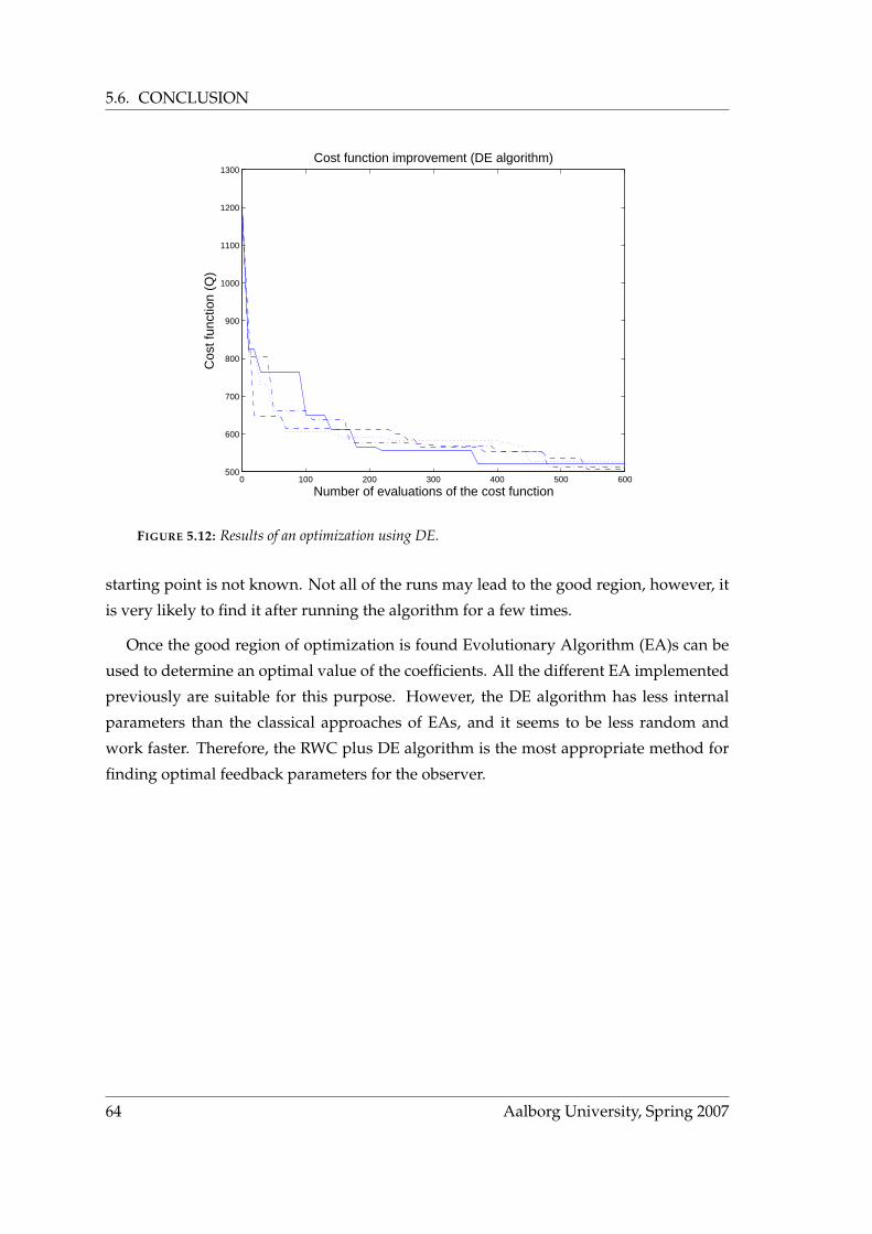
5.6. CONCLUSION
0 100 200 300 400 500 600500
600
700
800
900
1000
1100
1200
1300Cost function improvement (DE algorithm)
Number of evaluations of the cost function
Cos
t fun
ctio
n (Q
)
FIGURE 5.12: Results of an optimization using DE.
starting point is not known. Not all of the runs may lead to the good region, however, it
is very likely to find it after running the algorithm for a few times.
Once the good region of optimization is found Evolutionary Algorithm (EA)s can be
used to determine an optimal value of the coefficients. All the different EA implemented
previously are suitable for this purpose. However, the DE algorithm has less internal
parameters than the classical approaches of EAs, and it seems to be less random and
work faster. Therefore, the RWC plus DE algorithm is the most appropriate method for
finding optimal feedback parameters for the observer.
64 Aalborg University, Spring 2007

6VERIFICATION OF THEOBSERVER
The purpose of this chapter is to test the new hybrid observer developed throughout this
report against real measurements. The observer as described in Chapter 4 on page 37 will
be first tested. It will be then shown that the accuracy of the estimates may be increased
by adding an extra correction. A test of the observer with this extra correction will be
run, and the results will be discussed.
6.1 TEST SETUP
The observer is implemented in Simulink R© , as shown in Figure 6.1. It can be noticed that
there is an extra block called "proportional correction", it is to improve the precision of the
estimates, it will be described later on. The sampling period used for the system is chosen
to be the same as the PWM period, i.e. Ts = TPWM = 6.25 · 10−5 [s]. The observer is now
using the feedback matrices found in the previous chapter. The optimization allowed to
reduce a lot the cost function, and therefore the new coefficients should be more efficient
than the coefficients used in previous work.
speed corrected
select speed
select angle
thetae
we
new_thetae
new_we
fcn
proportional correction
1
0.05s+1
low pass filter
active_ABC
Cont. State
Q
reset
location observer
uy
fcn estimation theta_e w_e
Din_ABC
duty cyclesi_AB
currents
Din_ABC
i_AB
w_e
Q
reset
Cont. State
continuous time observer
theta_e
angle corrected
active_ABC
actives
z
1
Feedback estimated speed
FIGURE 6.1: Simulink implementation of the new hybrid observer.
A test scenario is defined in order to check the behaviour in the whole range of speed
considered (ωr ∈ [500; 1000] [rpm]). This test scenario also allows to see how the observer
handles continuous change in the angular velocity. Under no load conditions (which is
Group 1032c 65

6.2. TEST RESULTS
the case here), the speed of the motor can be considered proportional to the input duty
cycle Din. For this test, Din, which represents the speed, is depicted in Figure 6.2.
0 1 2 3 4 5 6 7 8 90.5
0.52
0.54
0.56
0.58
0.6
0.62
0.64
0.66
0.68
0.7Test scenario of the final observer
Time [s]
Inpu
t dut
y cy
cle
Din
FIGURE 6.2: Evolution of the input duty cycle during the test of the observer.
The test is run off-line, the measurements are taken from the real BLDCM, and then
fed to the Simulink R© implementation of the observer.
6.2 TEST RESULTS
The observer that was derived in Chapter 4 on page 37 (without the proportional correc-
tion) is tested against real measurements, Figures 6.3 on the facing page and 6.4 on the
next page represent the accuracy of the estimates of the new observer.
A brief study of Figure 6.3 on the facing page and Figure 6.4 on the next page allows
to notice that there is a strong correlation between the mean value of the errors and the
current value of the angular velocity. This is because the feedback coefficients k1 to k14
and the parameters of the model are very dependent on the speed and are found for an
angular velocity around 500 [rpm]. Therefore it is needed to have an additional correction
of the estimates if the speed is different from 500 [rpm].
66 Aalborg University, Spring 2007
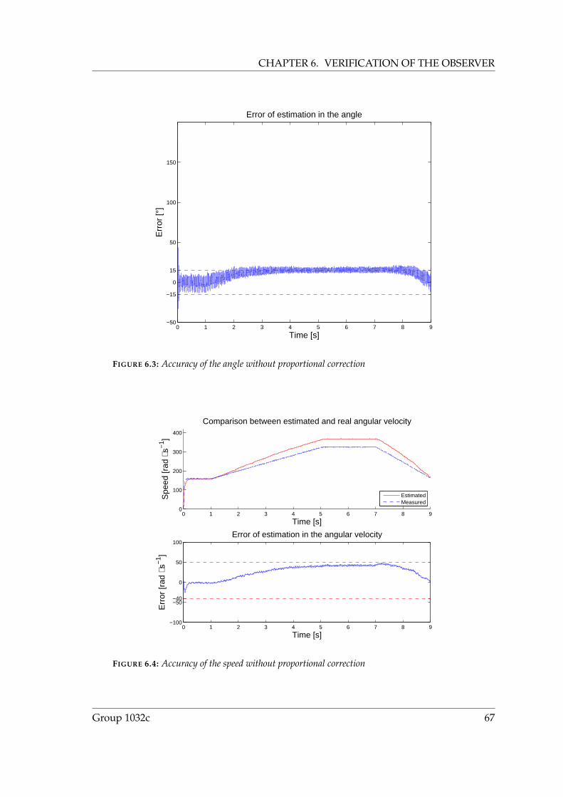
CHAPTER 6. VERIFICATION OF THE OBSERVER
0 1 2 3 4 5 6 7 8 9−50
−15
0
15
50
100
150
Error of estimation in the angle
Time [s]
Err
or [°
]
FIGURE 6.3: Accuracy of the angle without proportional correction
0 1 2 3 4 5 6 7 8 90
100
200
300
400
Comparison between estimated and real angular velocity
Time [s]
Spe
ed [r
ad ⋅
s−1 ]
EstimatedMeasured
0 1 2 3 4 5 6 7 8 9−100
−50−40
0
50
100Error of estimation in the angular velocity
Time [s]
Err
or [r
ad ⋅
s−1 ]
FIGURE 6.4: Accuracy of the speed without proportional correction
Group 1032c 67

6.3. PROPORTIONAL CORRECTION OF THE ESTIMATES
6.3 PROPORTIONAL CORRECTION OF THE ESTIMATES
The accuracy of the estimates may be increased by a proportional correction of ωe and
θe. The purpose is to compensate for the changes in the time varying parameter ωe. The
mean values of the errors are proportional to the current speed, therefore the corrected
estimates ωc and θc are defined as follows:
ωc = ωe − α(ωe − 160)
θc = θe − β(ωe − 160)(6.1)
ωe = 160 [rad · s−1] is the reference speed, it is equivalent to ωr = 500 [rpm], at this
speed no correction is needed. The correction applied depends on how far the current
speed is from the reference speed. The parameters α and β are calculated on basis of
Figure 6.3 on the preceding page and 6.4 on the previous page as they are the slope of the
error as a function of the speed. It is calculated α = 0.24 [] and β = 0.0015 [ radrad/s ].
0 1 2 3 4 5 6 7 8 9−50
−100
10
50
100
Error of estimation in the angle
Time [s]
Err
or [°
]
FIGURE 6.5: Error of estimation in the rotor angle.
The advantage of this type of correction is that it is easy to implement, and it requires
a reduced the number of calculations. Another advantage of this correction is that it is
very easy to tune, as there is only one coefficient per estimate, which can be changed to
68 Aalborg University, Spring 2007
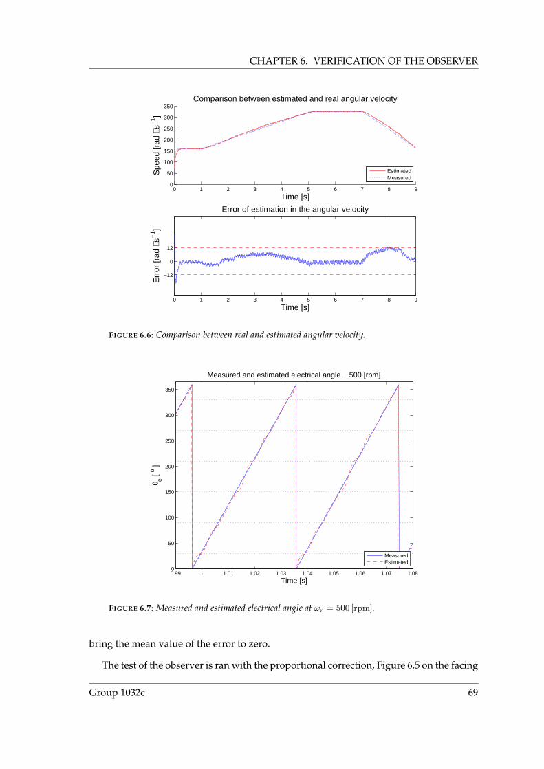
CHAPTER 6. VERIFICATION OF THE OBSERVER
0 1 2 3 4 5 6 7 8 90
50
100
150
200
250
300
350Comparison between estimated and real angular velocity
Time [s]
Spe
ed [r
ad ⋅
s−1 ]
EstimatedMeasured
0 1 2 3 4 5 6 7 8 9
−12
0
12
Error of estimation in the angular velocity
Time [s]
Err
or [r
ad ⋅
s−1 ]
FIGURE 6.6: Comparison between real and estimated angular velocity.
0.99 1 1.01 1.02 1.03 1.04 1.05 1.06 1.07 1.080
50
100
150
200
250
300
350
Measured and estimated electrical angle − 500 [rpm]
Time [s]
θ e [ o ]
MeasuredEstimated
FIGURE 6.7: Measured and estimated electrical angle at ωr = 500 [rpm].
bring the mean value of the error to zero.
The test of the observer is ran with the proportional correction, Figure 6.5 on the facing
Group 1032c 69
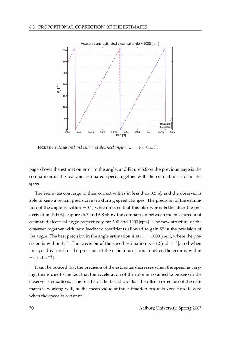
6.3. PROPORTIONAL CORRECTION OF THE ESTIMATES
6.005 6.01 6.015 6.02 6.025 6.03 6.035 6.04 6.045 6.050
50
100
150
200
250
300
350
Measured and estimated electrical angle − 1000 [rpm]
Time [s]
θ e [ o ]
MeasuredEstimated
FIGURE 6.8: Measured and estimated electrical angle at ωr = 1000 [rpm].
page shows the estimation error in the angle, and Figure 6.6 on the previous page is the
comparison of the real and estimated speed together with the estimation error in the
speed.
The estimates converge to their correct values in less than 0.2 [s], and the observer is
able to keep a certain precision even during speed changes. The precision of the estima-
tion of the angle is within ±10, which means that this observer is better than the one
derived in [NP06]. Figures 6.7 and 6.8 show the comparison between the measured and
estimated electrical angle respectively for 500 and 1000 [rpm]. The new structure of the
observer together with new feedback coefficients allowed to gain 5 in the precision of
the angle. The best precision in the angle estimation is at ωr = 1000 [rpm], where the pre-
cision is within ±3. The precision of the speed estimation is ±12 [rad · s−1], and when
the speed is constant the precision of the estimation is much better, the error is within
±4 [rad · s−1].
It can be noticed that the precision of the estimates decreases when the speed is vary-
ing, this is due to the fact that the acceleration of the rotor is assumed to be zero in the
observer’s equations. The results of the test show that the offset correction of the esti-
mates is working well, as the mean value of the estimation errors is very close to zero
when the speed is constant.
70 Aalborg University, Spring 2007

CHAPTER 6. VERIFICATION OF THE OBSERVER
6.4 CONCLUSION
The observer has been tested against real measurements, those results allowed to im-
prove the quality of the estimates by adding an extra correction. The observer is now
more precise and less complex, which is one step toward a real time implementation of
the observer, and a test in closed loop situation. The observer uses two current sensors to
estimate the speed and the angle. In the next chapter a new observer using one current
sensor to estimate the angle and the speed will be derived.
Group 1032c 71

This page is left intentionally blank

7SINGLE SENSOR OBSERVER
The hybrid observer derived in the previous chapters requires the use of two current sen-
sors, i.e. the measures of ias and ibs. In this chapter, the previous observer will be modi-
fied in order to be able to estimate using only one current measurement. The advantage
of the use of a single sensor to estimate angle and speed is that the cost is reduced, and
the reliability of the system is improved as there are less elements likely to fail. If more
sensors are available, they can be used for fault detection purposes.
Two practical conditions for being able to estimate with a single sensor will be ex-
pressed. It will be shown that the first condition can be realized by the system that is
considered in this report. For the second condition to be realized however, a new hybrid
automaton for the observer will be derived. Then, the corresponding equations for the
observer will be expressed. Finally, the observer will be tested against real measurements
to check that it is still able to estimate correctly the angle and the speed of the rotor.
7.1 PRACTICAL REQUIREMENTS FOR THE USE OF ONE
SENSOR
To reduce the number of sensors used, the system and the observer should meet two
requirements:
• As the goal is to use one current measurement, there cannot be cases where the
observer needs two different measurements.
• There must be a measurable current from which value it is possible to express the
currents ias and ibs in all discrete states where they are needed.
It can be noticed in Equation 4.9 on page 41 that the first requirement is not fulfilled by
the double sensor observer. When all three phases are conducting (drain states), it needs
measures of ias and ibs, which can only be provided by two different current sensors. The
drain states are usually short (in terms of time), therefore they don’t have much influence
on the dynamics of the observer. In order to meet the first requirement, the idea is to
have only predictive behaviour of the observer during the drain states. To verify that it
is possible to have only predictive behaviour during drain states, the double sensor is
tested with the feedback parameters k1, k2, k3, k4, and k5 in Equation 4.10 on page 41 set
to 0. The performance is found to be satisfactory, despite a slight loss in precision.
Group 1032c 73
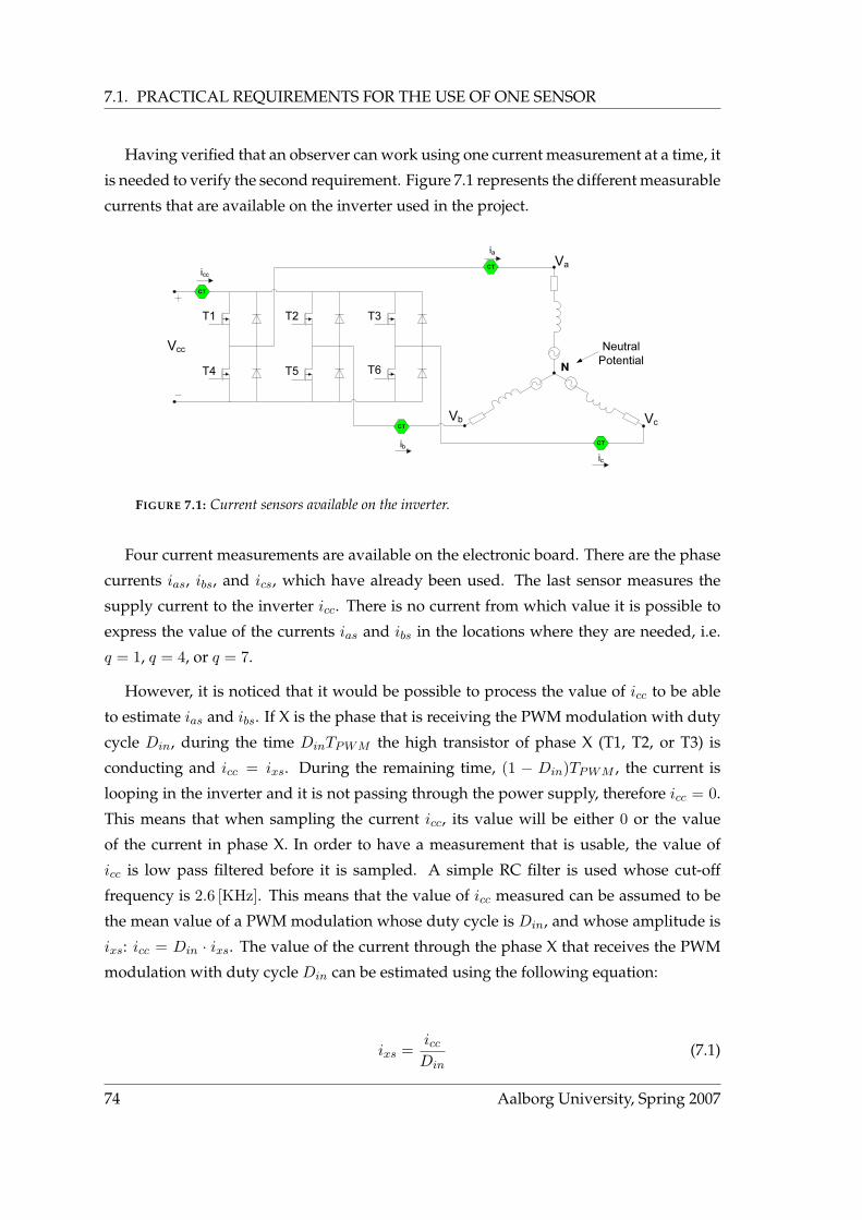
7.1. PRACTICAL REQUIREMENTS FOR THE USE OF ONE SENSOR
Having verified that an observer can work using one current measurement at a time, it
is needed to verify the second requirement. Figure 7.1 represents the different measurable
currents that are available on the inverter used in the project.
T2
T5
T3
T6
T1
T4
Vcc
Va
Vb Vc
Neutral Potential
ia
icib
CTiccCT
CT
CT
FIGURE 7.1: Current sensors available on the inverter.
Four current measurements are available on the electronic board. There are the phase
currents ias, ibs, and ics, which have already been used. The last sensor measures the
supply current to the inverter icc. There is no current from which value it is possible to
express the value of the currents ias and ibs in the locations where they are needed, i.e.
q = 1, q = 4, or q = 7.
However, it is noticed that it would be possible to process the value of icc to be able
to estimate ias and ibs. If X is the phase that is receiving the PWM modulation with duty
cycle Din, during the time DinTPWM the high transistor of phase X (T1, T2, or T3) is
conducting and icc = ixs. During the remaining time, (1 − Din)TPWM , the current is
looping in the inverter and it is not passing through the power supply, therefore icc = 0.
This means that when sampling the current icc, its value will be either 0 or the value
of the current in phase X. In order to have a measurement that is usable, the value of
icc is low pass filtered before it is sampled. A simple RC filter is used whose cut-off
frequency is 2.6 [KHz]. This means that the value of icc measured can be assumed to be
the mean value of a PWM modulation whose duty cycle is Din, and whose amplitude is
ixs: icc = Din · ixs. The value of the current through the phase X that receives the PWM
modulation with duty cycle Din can be estimated using the following equation:
ixs =iccDin
(7.1)
74 Aalborg University, Spring 2007
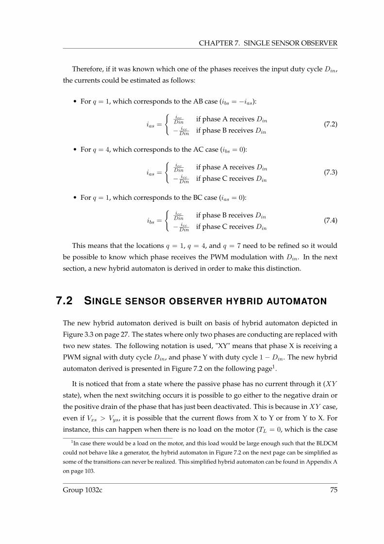
CHAPTER 7. SINGLE SENSOR OBSERVER
Therefore, if it was known which one of the phases receives the input duty cycle Din,
the currents could be estimated as follows:
• For q = 1, which corresponds to the AB case (ibs = −ias):
ias =
iccDin if phase A receives Din
− iccDin if phase B receives Din
(7.2)
• For q = 4, which corresponds to the AC case (ibs = 0):
ias =
iccDin if phase A receives Din
− iccDin if phase C receives Din
(7.3)
• For q = 1, which corresponds to the BC case (ias = 0):
ibs =
iccDin if phase B receives Din
− iccDin if phase C receives Din
(7.4)
This means that the locations q = 1, q = 4, and q = 7 need to be refined so it would
be possible to know which phase receives the PWM modulation with Din. In the next
section, a new hybrid automaton is derived in order to make this distinction.
7.2 SINGLE SENSOR OBSERVER HYBRID AUTOMATON
The new hybrid automaton derived is built on basis of hybrid automaton depicted in
Figure 3.3 on page 27. The states where only two phases are conducting are replaced with
two new states. The following notation is used, "XY" means that phase X is receiving a
PWM signal with duty cycle Din, and phase Y with duty cycle 1 −Din. The new hybrid
automaton derived is presented in Figure 7.2 on the following page1.
It is noticed that from a state where the passive phase has no current through it (XY
state), when the next switching occurs it is possible to go either to the negative drain or
the positive drain of the phase that has just been deactivated. This is because in XY case,
even if Vxs > Vys, it is possible that the current flows from X to Y or from Y to X. For
instance, this can happen when there is no load on the motor (TL = 0, which is the case
1In case there would be a load on the motor, and this load would be large enough such that the BLDCM
could not behave like a generator, the hybrid automaton in Figure 7.2 on the next page can be simplified as
some of the transitions can never be realized. This simplified hybrid automaton can be found in Appendix A
on page 103.
Group 1032c 75
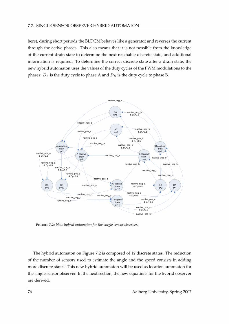
7.2. SINGLE SENSOR OBSERVER HYBRID AUTOMATON
here), during short periods the BLDCM behaves like a generator and reverses the current
through the active phases. This also means that it is not possible from the knowledge
of the current drain state to determine the next reachable discrete state, and additional
information is required. To determine the correct discrete state after a drain state, the
new hybrid automaton uses the values of the duty cycles of the PWM modulations to the
phases: DA is the duty cycle to phase A and DB is the duty cycle to phase B.
ABq=2
ACq=6
BCq=9
C positive drainq=12
C negative drainq=11
A negative drainq=7
A positive drainq=8
B positive drainq=3
B negative drainq=4
nactive_neg_a
nactive_neg_b & DA<0.5
nactive_pos_a
nactive_pos_b & DA>0.5
nactive_neg_b
nactive_pos_b
nactive_neg_c & DA>0.5
nactive_pos_c & DA<0.5
nactive_neg_c
nactive_neg_a & DB>0.5 nactive_pos_a
& DB<0.5
nactive_pos_c
nactive_pos_a
nactive_neg_b
nactive_pos_b
nactive_neg_a
nactive_neg_c
nactive_pos_c
BAq=1
CAq=5
CBq=10
nactive_neg_b
nactive_pos_b
nactive_neg_cnactive_pos_c
nactive_pos_a
nactive_neg_a
nactive_pos_c & DA>0.5
nactive_neg_c & DA<0.5
nactive_neg_b & DA>0.5
nactive_pos_b & DA<0.5
nactive_pos_a & DB>0.5
nactive_pos_a & DB<0.5
FIGURE 7.2: New hybrid automaton for the single sensor observer.
The hybrid automaton on Figure 7.2 is composed of 12 discrete states. The reduction
of the number of sensors used to estimate the angle and the speed consists in adding
more discrete states. This new hybrid automaton will be used as location automaton for
the single sensor observer. In the next section, the new equations for the hybrid observer
are derived.
76 Aalborg University, Spring 2007

CHAPTER 7. SINGLE SENSOR OBSERVER
7.3 SINGLE SENSOR OBSERVER EQUATIONS
The equations for the single sensor observer are very similar to the equations of the two
sensors observer described in Section 4.4 on page 41. The differences are that there is no
feedback in ABC case, and that the measurement of icc is used instead of the measure-
ments of ias and ibs.
It is recalled from Chapter 4 that ∆i =
[ias − ias
ibs − ibs
]. As the measurements of ias and
ibs are not available, there is: ∆i =
[ias − qf1(icc)
ibs − qf2(icc)
], where qf1(icc) and qf2(icc) are the
expressions of ias and ibs as functions of icc, depending on the discrete state. qf1(icc)
and qf2(icc) are defined by Equations 7.2, 7.3, and 7.4 on page 75. The new observer’s
equations are as follows:
• Drain cases
When all the phases conduct current, i.e. q ∈ 3, 4, 7, 8, 11, 12 the observer equa-
tions are run in open-loop, i.e. without feedback correction:
˙xq =
[− rs
LsI2×2 −λ′m
LsM′′
0 Jωe
]xq +
[1
LsM′
0
]Vabcs (7.5)
where
M′ =
[23 −1
3 −13
−13
23 −1
3
], M′′ =
[1 0
−12
√3
2
], J =
[0 −1
1 0
].
• BA case
This is the case when phase C is passive and phase B receives Din, i.e. q = 1. In
that case, ias = − iccDin and ibs = icc
Din , replacing the value of the measurements in ∆i,
leads to the new observer’s equation:
˙x1 =
[− rs
LsI2×2 −λ′m
Ls
1M′′
0 Jωe
]x1 +
[1
Ls
1M′
0
]Vabcs + 1K
[ias + icc
Din
ibs − iccDin
](7.6)
where
Group 1032c 77

7.3. SINGLE SENSOR OBSERVER EQUATIONS
1M′ =
[12 −1
2 0
−12
12 0
], 1M′′ =
[34 −
√3
4
−34
√3
4
], 1K =
k6 0
0 k7
k8 0
k9 0
.
• AB case
This is the case when phase C is passive and phase A receives Din, i.e. q = 2. In
that case, ias = iccDin and ibs = − icc
Din , replacing the value of the measurements in ∆i,
leads to the new observer’s equation:
˙x1 =
[− rs
LsI2×2 −λ′m
Ls
1M′′
0 Jωe
]x1 +
[1
Ls
1M′
0
]Vabcs + 1K
[ias − icc
Din
ibs + iccDin
](7.7)
where
1M′ =
[12 −1
2 0
−12
12 0
], 1M′′ =
[34 −
√3
4
−34
√3
4
], 1K =
k6 0
0 k7
k8 0
k9 0
.
• CA case
When phase B is passive and phase C receives Din, i.e. q = 5, ias = − iccDin and
ibs = 0. Since the current ibs is zero, it is not used in the feedback correction. The
observer’s equation is as follows:
˙x4 =
[− rs
Ls0
0 0
]−λ′m
Ls
4M′′
0 Jωe
x4 +
[1
Ls
4M′
0
]Vabcs + 4K
[ias + icc
Din
0
](7.8)
where
4M′ =
[12 0 −1
2
0 0 0
], 4M′′ =
[34
√3
4
0 0
], 4K =
k10 0
0 0
k11 0
k12 0
.
78 Aalborg University, Spring 2007

CHAPTER 7. SINGLE SENSOR OBSERVER
• AC case
Phase B is passive and phase A receives Din, i.e. q = 6. In that case ias = iccDin and
ibs = 0. The observer’s equation is as follows:
˙x4 =
[− rs
Ls0
0 0
]−λ′m
Ls
4M′′
0 Jωe
x4 +
[1
Ls
4M′
0
]Vabcs + 4K
[ias − icc
Din
0
](7.9)
where
4M′ =
[12 0 −1
2
0 0 0
], 4M′′ =
[34
√3
4
0 0
], 4K =
k10 0
0 0
k11 0
k12 0
.
• BC case
In that case, phase A is passive and phase B receives Din, i.e. q = 9. ias = 0,
therefore there is no correction on its basis, and ibs = iccDin . The observer’s equation
is as follows:
˙x7 =
[
0 0
0 − rsLs
]−λ′m
Ls
7M′′
0 Jωe
x7+
[1
Ls
7M′
0
]Vabcs+7K
[0
ibs − iccDin
](7.10)
where
7M′ =
[0 0 0
0 12 −1
2
], 7M′′ =
[0 0
0√
32
], 7K =
0 0
0 k13
0 0
0 k14
.
• CB case
In that case, phase A is passive and phase C receives Din, i.e. q = 10. ias = 0 and
ibs = − iccDin . The observer’s equation is as follows:
Group 1032c 79

7.4. TEST OF THE SINGLE SENSOR OBSERVER
˙x7 =
[
0 0
0 − rsLs
]−λ′m
Ls
7M′′
0 Jωe
x7+
[1
Ls
7M′
0
]Vabcs+7K
[0
ibs + iccDin
](7.11)
where
7M′ =
[0 0 0
0 12 −1
2
], 7M′′ =
[0 0
0√
32
], 7K =
0 0
0 k13
0 0
0 k14
.
Having the location automaton and the continuous time equations, the single sensor
observer will be tested against real measurements in the next section.
7.4 TEST OF THE SINGLE SENSOR OBSERVER
The single sensor observer is implemented in Simulink R©, as it was done for the previous
observer. In order to test this new observer, it is needed to take new measurements on
the real BLDCM as the value of icc is needed instead of ias and ibs. As the structure of
the single sensor observer is different from the structure of the double sensor observer,
the feedback gains are re-optimized using the feedback parameters of the double sensor
observer as a starting point. The optimization problem is in R9 while it was in R14 for the
optimization of the feedback parameters of the double sensor observer. This is due to the
fact that the five feedback coefficients for the drain states are not used in the single sensor
observer. Three additional dimensions are introduced without increasing the complexity
of the problem compared to the optimization of the double sensor observer, the problem
is now in R12. Those three new dimensions correspond to the electrical parameters of the
model (rs, Ls, λ′m), which means that they are also optimized. The advantage is that the
electrical parameters will be optimized instead of being estimated, which should provide
better results.
The test setup used for the test of the single sensor observer is the same as the test of
the regular observer in Chapter 6 on page 65, i.e. an acceleration and then a deceleration
of the motor through the whole range of speed considered in this project. Figure 7.3 on
the next page represents the estimation error in the angle during the test, and Figure 7.4
80 Aalborg University, Spring 2007
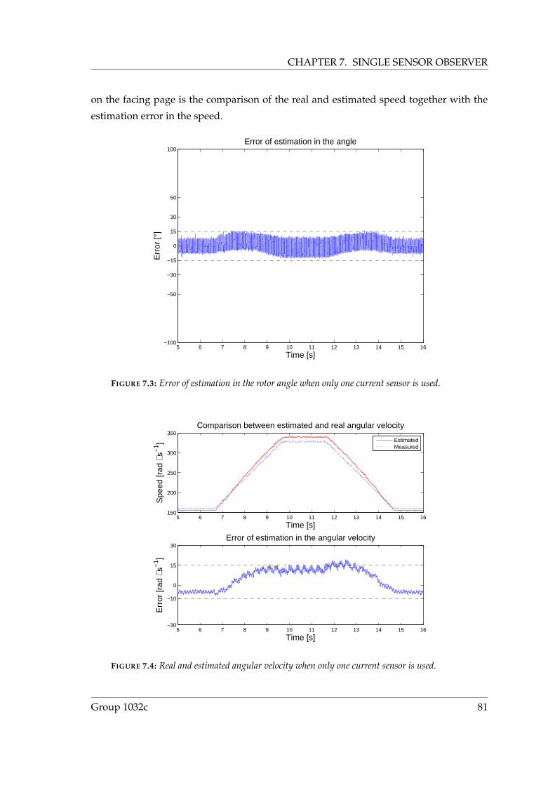
CHAPTER 7. SINGLE SENSOR OBSERVER
on the facing page is the comparison of the real and estimated speed together with the
estimation error in the speed.
5 6 7 8 9 10 11 12 13 14 15 16−100
−50
−30
−15
0
15
30
50
100Error of estimation in the angle
Time [s]
Err
or [°
]
FIGURE 7.3: Error of estimation in the rotor angle when only one current sensor is used.
5 6 7 8 9 10 11 12 13 14 15 16150
200
250
300
350Comparison between estimated and real angular velocity
Time [s]
Spe
ed [r
ad ⋅
s−1 ]
EstimatedMeasured
5 6 7 8 9 10 11 12 13 14 15 16−30
−10
0
15
30Error of estimation in the angular velocity
Time [s]
Err
or [r
ad ⋅
s−1 ]
FIGURE 7.4: Real and estimated angular velocity when only one current sensor is used.
Group 1032c 81
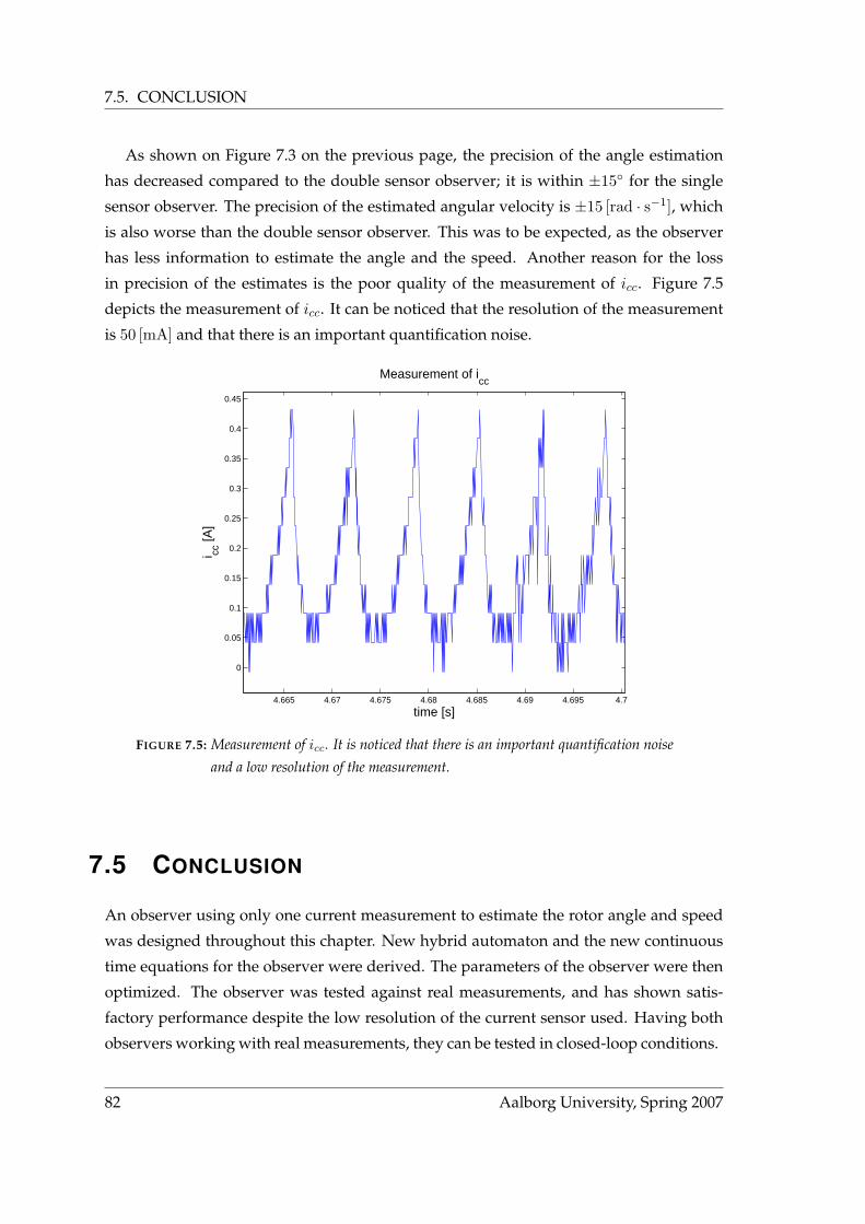
7.5. CONCLUSION
As shown on Figure 7.3 on the previous page, the precision of the angle estimation
has decreased compared to the double sensor observer; it is within ±15 for the single
sensor observer. The precision of the estimated angular velocity is ±15 [rad · s−1], which
is also worse than the double sensor observer. This was to be expected, as the observer
has less information to estimate the angle and the speed. Another reason for the loss
in precision of the estimates is the poor quality of the measurement of icc. Figure 7.5
depicts the measurement of icc. It can be noticed that the resolution of the measurement
is 50 [mA] and that there is an important quantification noise.
4.665 4.67 4.675 4.68 4.685 4.69 4.695 4.7
0
0.05
0.1
0.15
0.2
0.25
0.3
0.35
0.4
0.45
time [s]
i cc [A
]
Measurement of icc
FIGURE 7.5: Measurement of icc. It is noticed that there is an important quantification noise
and a low resolution of the measurement.
7.5 CONCLUSION
An observer using only one current measurement to estimate the rotor angle and speed
was designed throughout this chapter. New hybrid automaton and the new continuous
time equations for the observer were derived. The parameters of the observer were then
optimized. The observer was tested against real measurements, and has shown satis-
factory performance despite the low resolution of the current sensor used. Having both
observers working with real measurements, they can be tested in closed-loop conditions.
82 Aalborg University, Spring 2007

8CLOSED LOOPIMPLEMENTATION
In this chapter, the observers are tested under closed loop conditions and their usability
is asserted. Those tests determine the possible applications of the observers, for instance
control of a BLDCM, or fault detection applications.
Before the observers are tested in closed loop, they are reworked so that they can esti-
mate online. The reduction of the computational complexity of the observers is described
in Appendix B on page 105.
8.1 SIMULATIONS OF CLOSED LOOP PERFORMANCE
Before testing the observers on the real BLDCM, it is verified that they are able to work
in closed loop in simulations. Those simulations should reveal whether the observers
behave stable in closed loop and if there is a chance to use them on a real motor.
The simulations are conducted as shown in Figure 8.1. Since the observers cannot run
from the initial point, where the angular velocity is zero, there must be an initialization
procedure. In the case of simulations, the motor model is used as it would have feedback
from a position encoder. After 0.5 [s] the feedback is switched and from that moment, the
estimated angle is used to control the motor.
Model
Observer
ias, ibs
Commutator(PWM)
SW
u
θest
θmod
Comp
areθ a
nd ω
Din
θest,ωest
θmod
θcontrol
FIGURE 8.1: Block diagram of simulation procedure to verify the closed loop performance.
Switch SW is activated after 0.5 [s] to feed the estimated angle to the commutator
instead of the modelled angle.
In the simulations, the same test signal as in the verification of the observer is used, i.e.
an acceleration to the maximum speed (1000 [rpm]), and a deceleration to the minimum
speed (500 [rpm]). Since the scenario tests the whole range of speeds, it verifies in which
regions of speed the observers can work in closed loop.
Group 1032c 83
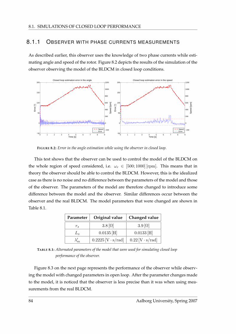
8.1. SIMULATIONS OF CLOSED LOOP PERFORMANCE
8.1.1 OBSERVER WITH PHASE CURRENTS MEASUREMENTS
As described earlier, this observer uses the knowledge of two phase currents while esti-
mating angle and speed of the rotor. Figure 8.2 depicts the results of the simulation of the
observer observing the model of the BLDCM in closed loop conditions.
−200
0
200
400
600
800
1000
1200
Spe
ed [r
pm]
0 1 2 3 4 5 6 7 8 9−50
0
50
100
150
200
Err
or [°
]
Closed loop estimation error in the angle
Time [s]
SpeedError
−200
0
200
400
600
800
1000
1200
Spe
ed [r
pm]
0 1 2 3 4 5 6 7 8 9−50
0
50
100
150
200
Err
or [°
]
Closed loop estimation error in the speed
Time [s]
SpeedError
FIGURE 8.2: Error in the angle estimation while using the observer in closed loop.
This test shows that the observer can be used to control the model of the BLDCM on
the whole region of speed considered, i.e. ωr ∈ [500; 1000] [rpm]. This means that in
theory the observer should be able to control the BLDCM. However, this is the idealized
case as there is no noise and no difference between the parameters of the model and those
of the observer. The parameters of the model are therefore changed to introduce some
difference between the model and the observer. Similar differences occur between the
observer and the real BLDCM. The model parameters that were changed are shown in
Table 8.1.
Parameter Original value Changed value
rs 3.8 [Ω] 3.9 [Ω]
Ls 0.0135 [H] 0.0133 [H]
λ′m 0.2225 [V · s/rad] 0.22 [V · s/rad]
TABLE 8.1: Alternated parameters of the model that were used for simulating closed loop
performance of the observer.
Figure 8.3 on the next page represents the performance of the observer while observ-
ing the model with changed parameters in open loop. After the parameter changes made
to the model, it is noticed that the observer is less precise than it was when using mea-
surements from the real BLDCM.
84 Aalborg University, Spring 2007
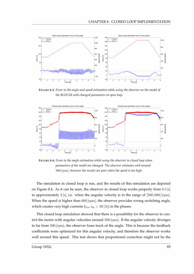
CHAPTER 8. CLOSED LOOP IMPLEMENTATION
−200
0
200
400
600
800
1000
1200
Spe
ed [r
pm]
0 1 2 3 4 5 6 7 8 9−50
0
50
100
150
200E
rror
[°]
Open loop estimation error in the angle
Time [s]
SpeedError
0
200
400
600
800
1000
Spe
ed [r
pm]
0 1 2 3 4 5 6 7 8 9−20
0
20
40
60
80
100
120
140
160
180
Err
or [°
]
Open loop estimation error in the speed
Time [s]
SpeedError
FIGURE 8.3: Error in the angle and speed estimation while using the observer on the model of
the BLDCM with changed parameters in open loop.
0
200
400
600
800
1000
Spe
ed [r
pm]
0 1 2 3 4 5 6 7 8 9−20
0
20
40
60
80
100
120
140
160
180
Err
or [°
]
Closed loop estimation error in the angle
Time [s]
SpeedError
0
200
400
600
800
1000
Spe
ed [r
pm]
0 1 2 3 4 5 6 7 8 9−20
0
20
40
60
80
100
120
140
160
180
Err
or [°
]
Closed loop estimation error in the speed
Time [s]
SpeedError
FIGURE 8.4: Error in the angle estimation while using the observer in closed loop when
parameters of the model are changed. The observer estimates well around
500 [rpm], however the results are poor when the speed is too high.
The simulation in closed loop is run, and the results of this simulation are depicted
on Figure 8.4. As it can be seen, the observer in closed loop works properly from 0.5 [s]
to approximately 2 [s], i.e. when the angular velocity is in the range of [500; 600] [rpm].
When the speed is higher than 600 [rpm], the observer provides wrong switching angle,
which creates very high currents (ias, ibs > 20 [A]) in the phases.
This closed loop simulation showed that there is a possibility for the observer to con-
trol the motor with angular velocities around 500 [rpm]. If the angular velocity diverges
to far from 500 [rpm], the observer loses track of the angle. This is because the feedback
coefficients were optimized for this angular velocity, and therefore the observer works
well around this speed. This test shows that proportional correction might not be the
Group 1032c 85

8.2. OBSERVER TESTS ON THE REAL SYSTEM
best way to handle large changes in the angular velocity when operating in closed loop.
The range of speed where the observer works properly ([500; 600] [rpm]) is reduced com-
pared to the range of speed that was considered in this project ([500; 1000] [rpm]).
Better results are expected during the closed loop test with the real motor since the
introduced parameter perturbations are likely to be to large. Particularly, the range of
speed where the observer can run in closed loop should be larger, and the precision of
the angle estimate should increase.
8.1.2 SINGLE SENSOR OBSERVER
This observer uses only one current sensor (icc current) to estimate the angle and the
speed of the rotor. The particularity of this observer is that there is no feedback correction
in the three phase cases (drain states). For the purpose of the simulation, the current icc is
computed on basis of the two phase currents ias and ibs that are the outputs of the model.
This value is then fed to the single sensor observer, and its behaviour under closed loop
conditions is tested in the same way as for the classical observer.
The results of the simulations of the single sensor observer is that it is not able to
estimate correctly the angle of the rotor in closed loop conditions. However, the observer
was not tuned to work with the model but with the real motor, therefore better results
might be obtained during the closed loop test with the real BLDCM.
8.2 OBSERVER TESTS ON THE REAL SYSTEM
The simulations of the observers in closed loop have shown that the two sensors ob-
server could be used to provide the information of the angle to replace the encoder for
the control of the real BLDCM. The single sensor observer, however, has not shown good
performance in closed loop operation in simulations. The double sensor observer will
be tested first. Having shown that the double sensor observer works in closed loop, the
single sensor observer will be tested to verify the results obtained during closed loop
simulations. The test setup for the closed loop tests with the real motor is shown on Fig-
ure 8.5 on the next page. It is the same setup as for the simulations only the model is
replaced with the real motor and the outputs are measured with sensors.
86 Aalborg University, Spring 2007

CHAPTER 8. CLOSED LOOP IMPLEMENTATION
Observer
ias, ibs ,icc
Commutator(PWM)
SW
DA
θest
θencoder
Comp
areθ a
nd ω
Din
DC
DB
Encoder θencoder,ωencoder
θest,ωest
BLDCMInverterSensors
θcontrol
FIGURE 8.5: Test setup for the closed loop performance with the real BLDCM. SW chooses
which angle is fed to the commutator, it is controlled manually during the test.
8.2.1 TEST OF THE OBSERVER USING TWO CURRENT MEASURE-
MENTS
First it needs to be verified that the observer works properly in closed loop with constant
speed of 500 [rpm], which is the speed where the optimization was made, and therefore
where it is most probable to work. Then, the observer will be tested with smooth changes
in the speed. This will allow to determine whether it can work properly when the angular
velocity varies, and in which range of speed.
Figure 8.6 on the following page, Figure 8.7 on the next page, and Figure 8.8 on page 89
depict the results of the closed-loop test with constant angular velocity. The observer
works properly at 500 [rpm], the error in the angle estimate is within ±15, and the error
in the speed estimate is approximately constant. Figure 8.6 on the next page shows that
there is a correlation between the estimate error in the angle and the fact that the observer
is used for the control. When it is used there is a slight decrease of the precision. It
is shown on Figure 8.8 on page 89 that there is also a link between the amplitude of
the currents and the fact that the observer is used for the control. The amplitude of the
currents increase when operating with the observer. This is because the switching angle
is not precisely 90 but 90±15, which changes the amplitude of the currents. As it can be
noticed on Figure 8.7 on the next page, the consequence of this change in the amplitude
of the currents is that there are irregular ripples in the angular velocity of the BLDCM.
Having verified that the observer works in real conditions with constant angular ve-
locity, it can now be tested with smooth changes in speed. The test scenario is, from
500 [rpm] an acceleration to a higher speed, then a steady state at this speed, and finally a
deceleration to 500 [rpm]. Several tests will be run with different values for the maximum
Group 1032c 87
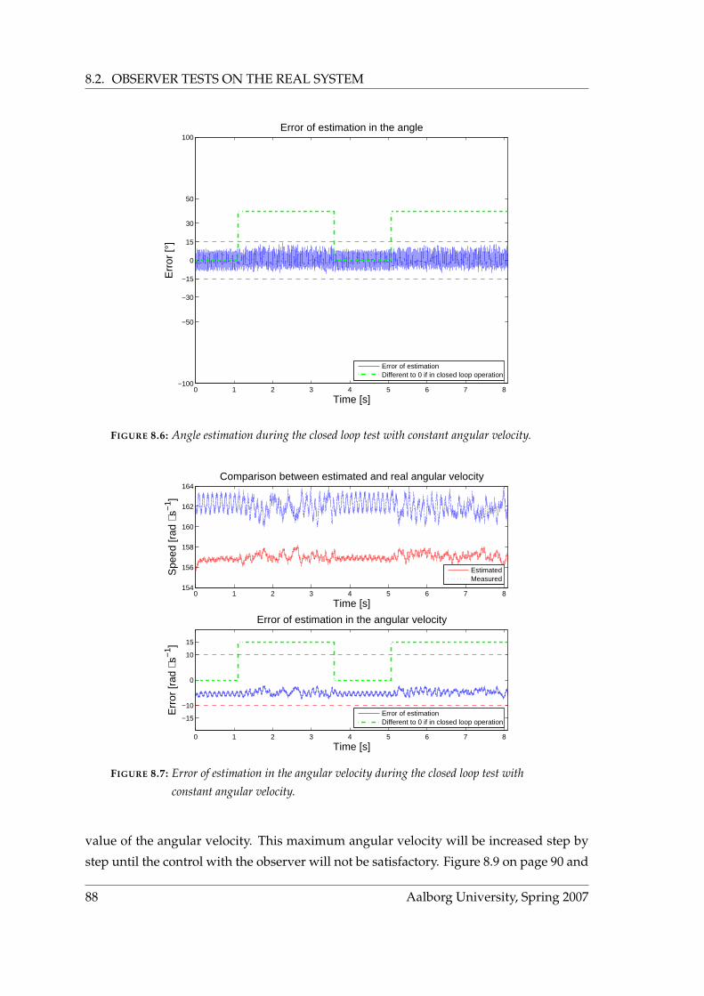
8.2. OBSERVER TESTS ON THE REAL SYSTEM
0 1 2 3 4 5 6 7 8−100
−50
−30
−15
0
15
30
50
100Error of estimation in the angle
Time [s]
Err
or [°
]
Error of estimationDifferent to 0 if in closed loop operation
FIGURE 8.6: Angle estimation during the closed loop test with constant angular velocity.
0 1 2 3 4 5 6 7 8154
156
158
160
162
164Comparison between estimated and real angular velocity
Time [s]
Spe
ed [r
ad ⋅
s−1 ]
EstimatedMeasured
0 1 2 3 4 5 6 7 8
−15
−10
0
10
15
Error of estimation in the angular velocity
Time [s]
Err
or [r
ad ⋅
s−1 ]
Error of estimationDifferent to 0 if in closed loop operation
FIGURE 8.7: Error of estimation in the angular velocity during the closed loop test with
constant angular velocity.
value of the angular velocity. This maximum angular velocity will be increased step by
step until the control with the observer will not be satisfactory. Figure 8.9 on page 90 and
88 Aalborg University, Spring 2007
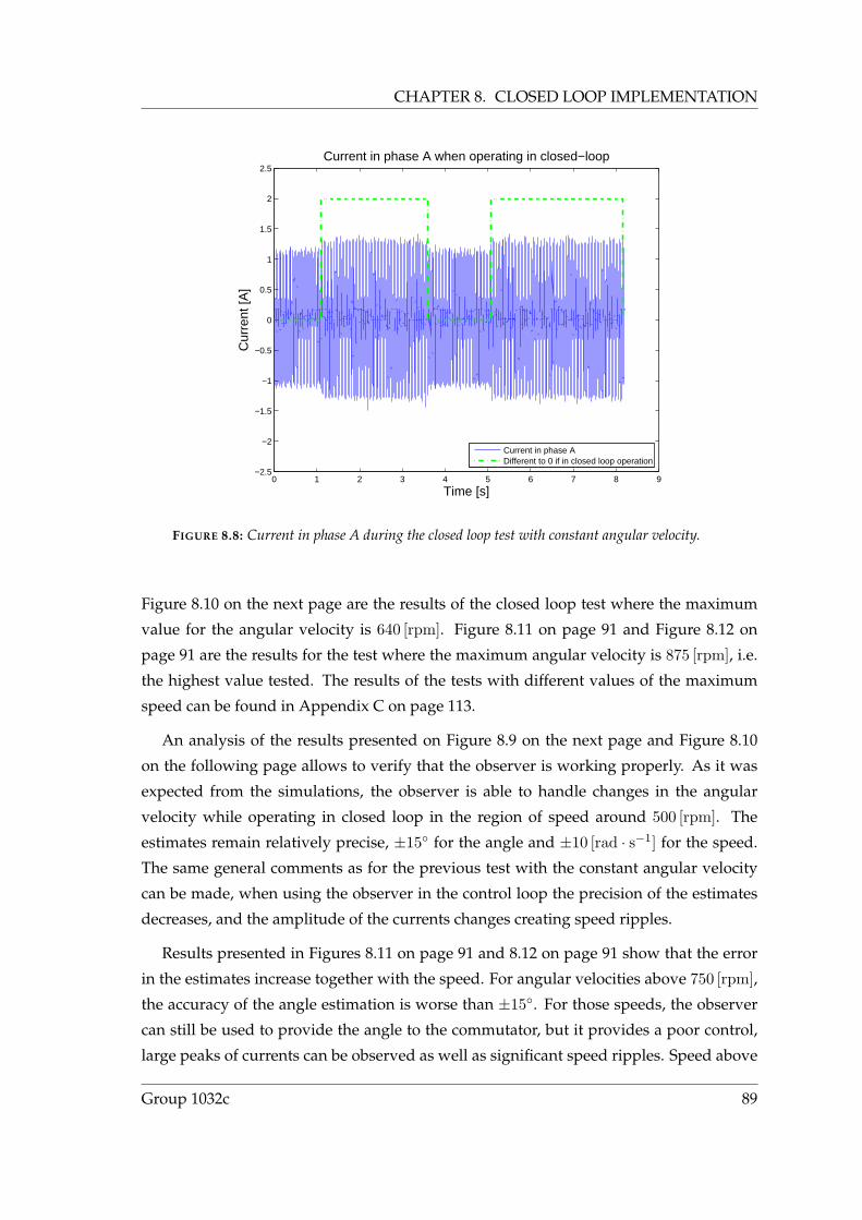
CHAPTER 8. CLOSED LOOP IMPLEMENTATION
0 1 2 3 4 5 6 7 8 9−2.5
−2
−1.5
−1
−0.5
0
0.5
1
1.5
2
2.5Current in phase A when operating in closed−loop
Time [s]
Cur
rent
[A]
Current in phase ADifferent to 0 if in closed loop operation
FIGURE 8.8: Current in phase A during the closed loop test with constant angular velocity.
Figure 8.10 on the next page are the results of the closed loop test where the maximum
value for the angular velocity is 640 [rpm]. Figure 8.11 on page 91 and Figure 8.12 on
page 91 are the results for the test where the maximum angular velocity is 875 [rpm], i.e.
the highest value tested. The results of the tests with different values of the maximum
speed can be found in Appendix C on page 113.
An analysis of the results presented on Figure 8.9 on the next page and Figure 8.10
on the following page allows to verify that the observer is working properly. As it was
expected from the simulations, the observer is able to handle changes in the angular
velocity while operating in closed loop in the region of speed around 500 [rpm]. The
estimates remain relatively precise, ±15 for the angle and ±10 [rad · s−1] for the speed.
The same general comments as for the previous test with the constant angular velocity
can be made, when using the observer in the control loop the precision of the estimates
decreases, and the amplitude of the currents changes creating speed ripples.
Results presented in Figures 8.11 on page 91 and 8.12 on page 91 show that the error
in the estimates increase together with the speed. For angular velocities above 750 [rpm],
the accuracy of the angle estimation is worse than ±15. For those speeds, the observer
can still be used to provide the angle to the commutator, but it provides a poor control,
large peaks of currents can be observed as well as significant speed ripples. Speed above
Group 1032c 89
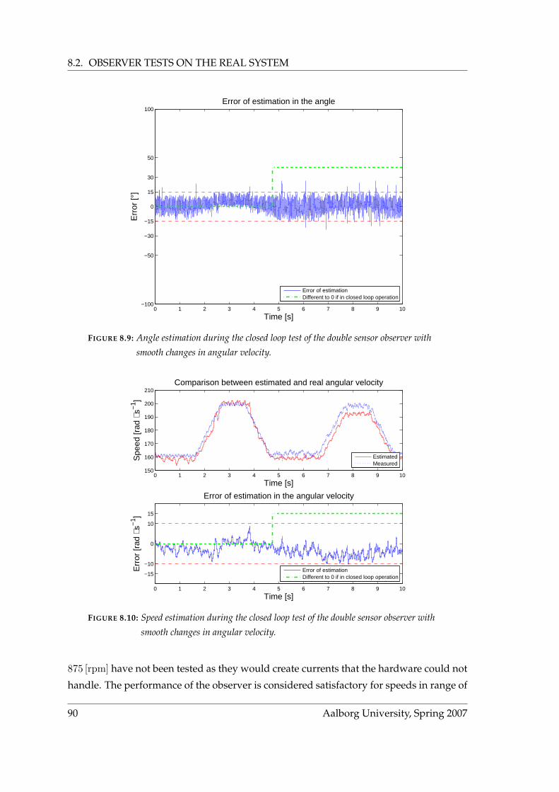
8.2. OBSERVER TESTS ON THE REAL SYSTEM
0 1 2 3 4 5 6 7 8 9 10−100
−50
−30
−15
0
15
30
50
100Error of estimation in the angle
Time [s]
Err
or [°
]
Error of estimationDifferent to 0 if in closed loop operation
FIGURE 8.9: Angle estimation during the closed loop test of the double sensor observer with
smooth changes in angular velocity.
0 1 2 3 4 5 6 7 8 9 10150
160
170
180
190
200
210Comparison between estimated and real angular velocity
Time [s]
Spe
ed [r
ad ⋅
s−1 ]
EstimatedMeasured
0 1 2 3 4 5 6 7 8 9 10
−15
−10
0
10
15
Error of estimation in the angular velocity
Time [s]
Err
or [r
ad ⋅
s−1 ]
Error of estimationDifferent to 0 if in closed loop operation
FIGURE 8.10: Speed estimation during the closed loop test of the double sensor observer with
smooth changes in angular velocity.
875 [rpm] have not been tested as they would create currents that the hardware could not
handle. The performance of the observer is considered satisfactory for speeds in range of
90 Aalborg University, Spring 2007
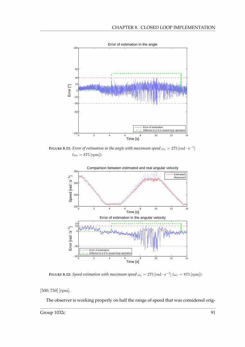
CHAPTER 8. CLOSED LOOP IMPLEMENTATION
0 2 4 6 8 10 12 14−100
−50
−30
−15
0
15
30
50
100Error of estimation in the angle
Time [s]
Err
or [°
]
Error of estimationDifferent to 0 if in closed loop operation
FIGURE 8.11: Error of estimation in the angle with maximum speed ωe = 275 [rad · s−1]
(ωr = 875 [rpm]).
0 2 4 6 8 10 12 14150
200
250
300Comparison between estimated and real angular velocity
Time [s]
Spe
ed [r
ad ⋅
s−1 ]
EstimatedMeasured
0 2 4 6 8 10 12 14−50
−30
0
1015
Error of estimation in the angular velocity
Time [s]
Err
or [r
ad ⋅
s−1 ]
Error of estimationDifferent to 0 if in closed loop operation
FIGURE 8.12: Speed estimation with maximum speed ωe = 275 [rad · s−1] (ωr = 875 [rpm]).
[500; 750] [rpm].
The observer is working properly on half the range of speed that was considered orig-
Group 1032c 91
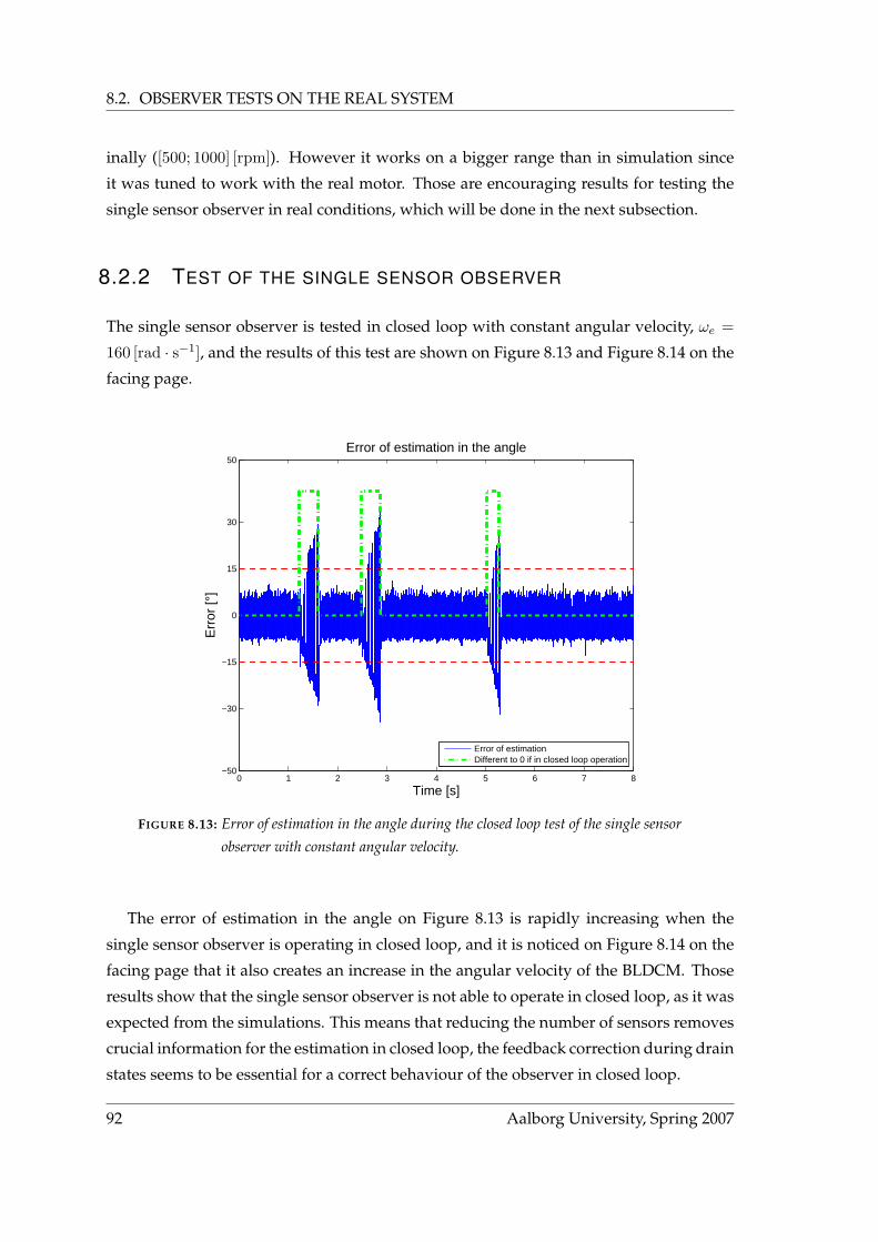
8.2. OBSERVER TESTS ON THE REAL SYSTEM
inally ([500; 1000] [rpm]). However it works on a bigger range than in simulation since
it was tuned to work with the real motor. Those are encouraging results for testing the
single sensor observer in real conditions, which will be done in the next subsection.
8.2.2 TEST OF THE SINGLE SENSOR OBSERVER
The single sensor observer is tested in closed loop with constant angular velocity, ωe =
160 [rad · s−1], and the results of this test are shown on Figure 8.13 and Figure 8.14 on the
facing page.
0 1 2 3 4 5 6 7 8−50
−30
−15
0
15
30
50Error of estimation in the angle
Time [s]
Err
or [°
]
Error of estimationDifferent to 0 if in closed loop operation
FIGURE 8.13: Error of estimation in the angle during the closed loop test of the single sensor
observer with constant angular velocity.
The error of estimation in the angle on Figure 8.13 is rapidly increasing when the
single sensor observer is operating in closed loop, and it is noticed on Figure 8.14 on the
facing page that it also creates an increase in the angular velocity of the BLDCM. Those
results show that the single sensor observer is not able to operate in closed loop, as it was
expected from the simulations. This means that reducing the number of sensors removes
crucial information for the estimation in closed loop, the feedback correction during drain
states seems to be essential for a correct behaviour of the observer in closed loop.
92 Aalborg University, Spring 2007
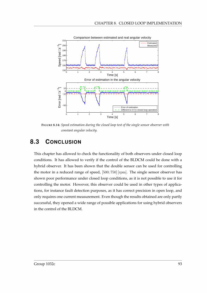
CHAPTER 8. CLOSED LOOP IMPLEMENTATION
0 1 2 3 4 5 6 7 8150
160
170
180
190
200
210Comparison between estimated and real angular velocity
Time [s]
Spe
ed [r
ad ⋅
s−1 ]
0 1 2 3 4 5 6 7 8
−50
−100
10
Error of estimation in the angular velocity
Time [s]
Err
or [r
ad ⋅
s−1 ]
EstimatedMeasured
Error of estimationDifferent to 0 if in closed loop operation
FIGURE 8.14: Speed estimation during the closed loop test of the single sensor observer with
constant angular velocity.
8.3 CONCLUSION
This chapter has allowed to check the functionality of both observers under closed loop
conditions. It has allowed to verify if the control of the BLDCM could be done with a
hybrid observer. It has been shown that the double sensor can be used for controlling
the motor in a reduced range of speed, [500; 750] [rpm]. The single sensor observer has
shown poor performance under closed loop conditions, as it is not possible to use it for
controlling the motor. However, this observer could be used in other types of applica-
tions, for instance fault detection purposes, as it has correct precision in open loop, and
only requires one current measurement. Even though the results obtained are only partly
successful, they opened a wide range of possible applications for using hybrid observers
in the control of the BLDCM.
Group 1032c 93

This page is left intentionally blank

9CONCLUSION
This chapter concludes the work done during the project. It presents the achievements
and compares them with the project requirements stated in the introduction. The most
important results and possible applications of the developed observer are gathered and
discussed. Future work possibilities are presented.
9.1 SUMMARY
This project was a continuation of previously conducted work on modelling and state
estimation for brushless DC motors using hybrid theory ([HB05], [Han06] and [NP06]).
It mostly relies on the development of a novel hybrid model and observer presented in
[NP06], where it was shown that there is a possibility of constructing a hybrid adaptive
observer that would estimate the rotor angle and speed based on two current measure-
ments. The goal stated in this project was to further improve the observer and verify its
usability in a real application. Such an observer could be potentially used in a various of
applications replacing some of the already known BLDCM control techniques.
It was shown in [NP06], that the observer tracks the rotor angle and speed very well,
but at that point it was not possible to verify it on a real system. The observer needed to
be optimized in a variety of ways.
Since it was very difficult to find the observer’s feedback coefficients, it was needed
to improve the optimization technique used for this purpose. Various techniques were
compared and it was found that the optimization should be done in two stages. First
stage would determine the region where the feedback coefficients are sufficiently close to
the optimal values. For this purpose the RWC algorithm was found to be very suitable.
In the second stage, the DE algorithm would be employed to find correct values of the
feedback gains. This algorithm benefits from gradient and evolutionary techniques and
requires a very limited number of internal parameters. Those parameters are easy to find
and they are not very crucial for the optimization.
The observer was very computational demanding the way it was implemented previ-
ously. Therefore, to ensure real time computation, it was necessary to lower the demands.
This was done by simplifying the equations (removing zero multiplications), removing
necessity of using Checkmate and Stateflow toolboxes. In the end, the computational de-
mands were lowered significantly and it was possible to run the observer on the dSpace R©
Group 1032c 95
9.2. METHODOLOGY
platform in real time.
An alternative version of the observer was also developed. In this observer the angular
position and speed were estimated using only one current measurement (DC current). A
novel hybrid automaton and novel equations were derived for this purpose.
The observers were tested against real measurements in open loop conditions and
have shown satisfactory performance. The double sensor observer has a precision of
±10 in the angle and a precision of ±12 [rad · s−1] in the speed, while the single sensor
observer has a precision of ±15 in the angle and a precision of ±15 [rad · s−1] in the
speed.
Both of the observers were then verified on the real system in closed loop. This was
preceded by series of simulations, that have shown that there is a possibility to use the
double sensor observer in the closed loop on the real motor. The one sensor observer
has shown poor performance in the simulations and real application. The double sensor
observer works well in closed loop, however the operating region is smaller than it was
expected. The functionality is sufficient between 500 and 750 [rpm] with a precision of
±15 and ±10 [rad · s−1].
Possible applications of the observers include fault detection, tolerant control and ad-
vanced control to remove the torque ripples. The observer may replace the encoder in
case of a fault or can be used to determine whether the fault has occurred. Further im-
provements of the hybrid adaptive observers may allow the control based on the estima-
tion instead of the back-EMF sensing.
9.2 METHODOLOGY
The method of developing the hybrid adaptive observer for a BLDCM presented in this
report consists of the following procedures:
1. Determine the internal parameters of the motor.
2. Implement the observer equations and hybrid automaton.
3. Acquire measurements from the BLDCM (speed step response) – two phase cur-
rents, rotor’s angle and inputs.
4. Use the measurements for the optimization of the feedback coefficients – find opti-
mization region with RWC algorithm and tune the coefficients with DE algorithm.
96 Aalborg University, Spring 2007

CHAPTER 9. CONCLUSION
5. Extend the performance of the observer on the operating region by one of the fol-
lowing methods:
(a) Determine the proportional correction coefficients.
(b) Repeat the optimization procedure for different rotation speeds in the operat-
ing region. Verify the dependencies between coefficients at various rotation
speeds and interpolate them on the whole operating region. This methods
requires more online and offline calculations.
9.3 ACHIEVEMENTS
The goal of the project, to verify the usability of the observer in the real application,
was achieved. The determination of the feedback coefficients through optimization was
analysed and improved. An observer that uses only one current sensor to estimate the
angular position and velocity of the rotor was developed.
The observers were tested in closed loop where the position encoder was replaced by
the estimate in order to determine the switching sequence of the transistors. Single sen-
sor observer has shown poor performance in closed loop and therefore its application
possibilities are limited compared to the double sensor observer. The double sensor ob-
server can be used to control the BLDCM with a precision of ±15 in a reduced range of
speed ωr ∈ [500; 750] [rpm]. The quality of the control using the double sensor observer is
slightly worse than when using the encoder (the amplitude of the currents increases and
the speed has larger ripples). The potential applications of such observers in the control
of a BLDCM are very broad.
9.4 FUTURE WORK
The estimation method using hybrid theory was verified and gave successfully results. It
was shown that the observer is suitable to operate in closed loop. However, the operating
region should be extended as it was smaller than the range of speed considered originally.
The influence of the motor load should be verified. It is expected that the observer would
perform better when the motor is running with a load. This is due to the fact that the
currents would be larger and easier to observe.
An observer that assumes both rotating directions should be implemented, so that the
Group 1032c 97

9.4. FUTURE WORK
motor can be controlled with positive or negative angular velocities. Additional feedback
correction could be used to verify if the accuracy of the observers can be improved by us-
ing integral feedback correction in addition to the proportional feedback. The parameters
of the model could be considered as time-varying parameters and estimated online. This
could improve the performance of the observers, as those parameters are dependent on
the angular velocity.
Advanced control methods should be used together with the observer, for instance to
reduce the torque ripples of the BLDCM. This study would allow to verify whether the
observer provides sufficient precision for those techniques.
A startup procedure should be designed in case the encoder would be completely
replaced by the observer. The motor could be running in an open loop and the loop
would be closed when the observer has converged.
The observer could be tested under various conditions to verify whether it can be
implemented in commercial applications. There are limited academic research tasks to
be done in order to improve it. The future work would concentrate on implementing the
observer for being used in real applications.
98 Aalborg University, Spring 2007
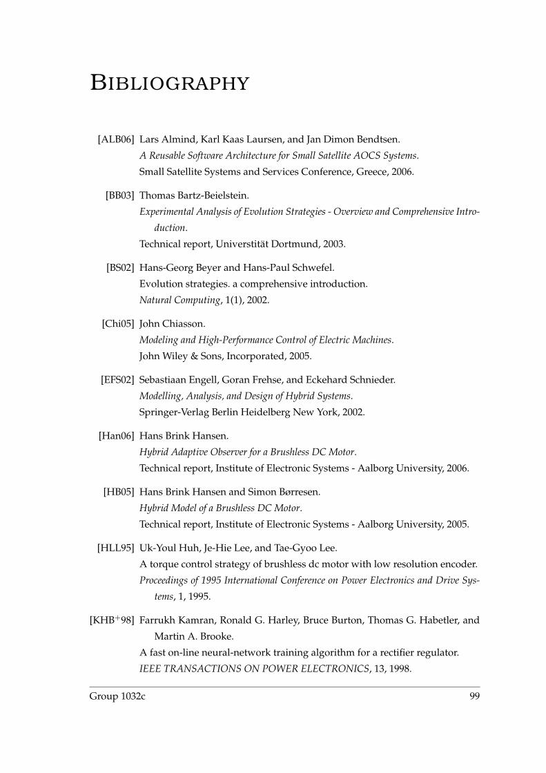
BIBLIOGRAPHY
[ALB06] Lars Almind, Karl Kaas Laursen, and Jan Dimon Bendtsen.
A Reusable Software Architecture for Small Satellite AOCS Systems.
Small Satellite Systems and Services Conference, Greece, 2006.
[BB03] Thomas Bartz-Beielstein.
Experimental Analysis of Evolution Strategies - Overview and Comprehensive Intro-
duction.
Technical report, Universtität Dortmund, 2003.
[BS02] Hans-Georg Beyer and Hans-Paul Schwefel.
Evolution strategies. a comprehensive introduction.
Natural Computing, 1(1), 2002.
[Chi05] John Chiasson.
Modeling and High-Performance Control of Electric Machines.
John Wiley & Sons, Incorporated, 2005.
[EFS02] Sebastiaan Engell, Goran Frehse, and Eckehard Schnieder.
Modelling, Analysis, and Design of Hybrid Systems.
Springer-Verlag Berlin Heidelberg New York, 2002.
[Han06] Hans Brink Hansen.
Hybrid Adaptive Observer for a Brushless DC Motor.
Technical report, Institute of Electronic Systems - Aalborg University, 2006.
[HB05] Hans Brink Hansen and Simon Børresen.
Hybrid Model of a Brushless DC Motor.
Technical report, Institute of Electronic Systems - Aalborg University, 2005.
[HLL95] Uk-Youl Huh, Je-Hie Lee, and Tae-Gyoo Lee.
A torque control strategy of brushless dc motor with low resolution encoder.
Proceedings of 1995 International Conference on Power Electronics and Drive Sys-
tems, 1, 1995.
[KHB+98] Farrukh Kamran, Ronald G. Harley, Bruce Burton, Thomas G. Habetler, and
Martin A. Brooke.
A fast on-line neural-network training algorithm for a rectifier regulator.
IEEE TRANSACTIONS ON POWER ELECTRONICS, 13, 1998.
Group 1032c 99
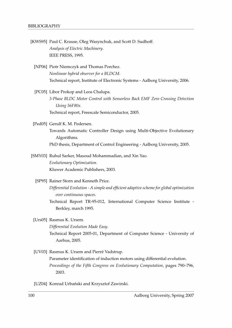
BIBLIOGRAPHY
[KWS95] Paul C. Krause, Oleg Wasynchuk, and Scott D. Sudhoff.
Analysis of Electric Machinery.
IEEE PRESS, 1995.
[NP06] Piotr Niemczyk and Thomas Porchez.
Nonlinear hybrid observer for a BLDCM.
Technical report, Institute of Electronic Systems - Aalborg University, 2006.
[PC05] Libor Prokop and Leos Chalupa.
3-Phase BLDC Motor Control with Sensorless Back EMF Zero Crossing Detection
Using 56F80x.
Technical report, Freescale Semiconductor, 2005.
[Ped05] Gerulf K. M. Pedersen.
Towards Automatic Controller Design using Multi-Objective Evolutionary
Algorithms.
PhD thesis, Department of Control Engineering - Aalborg University, 2005.
[SMY03] Ruhul Sarker, Masoud Mohammadian, and Xin Yao.
Evolutionary Optimization.
Kluwer Academic Publishers, 2003.
[SP95] Rainer Storn and Kenneth Price.
Differential Evolution - A simple and efficient adaptive scheme for global optimization
over continuous spaces.
Technical Report TR-95-012, International Computer Science Institute -
Berkley, march 1995.
[Urs05] Rasmus K. Ursem.
Differential Evolution Made Easy.
Technical Report 2005-01, Department of Computer Science - University of
Aarhus, 2005.
[UV03] Rasmus K. Ursem and Pierré Vadstrup.
Parameter identification of induction motors using differential evolution.
Proceedings of the Fifth Congress on Evolutionary Computation, pages 790–796,
2003.
[UZ04] Konrad Urbanski and Krzysztof Zawirski.
100 Aalborg University, Spring 2007

BIBLIOGRAPHY
Adaptive observer of rotor speed and position for pmsm sensorless control
system.
COMPEL: The International Journal for Computation and Mathematics in Electrical
and Electronic Engineering, 23, 2004.
[WQ05] Fang Wang and Yuhui Qiu.
Multimodal function optimizing by a new hybrid nonlinear simplex search
and particle swarm algorithm.
In ECML, pages 759–766, 2005.
Group 1032c 101

This page is left intentionally blank
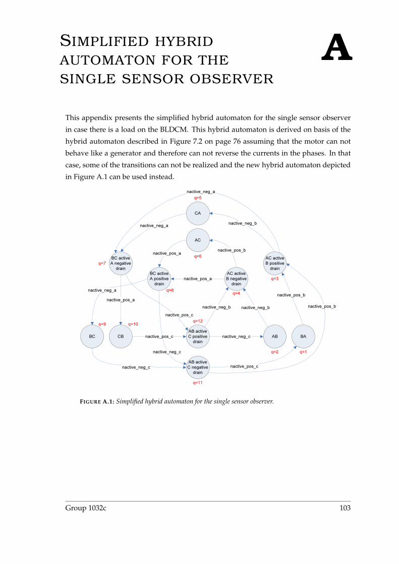
ASIMPLIFIED HYBRIDAUTOMATON FOR THESINGLE SENSOR OBSERVER
This appendix presents the simplified hybrid automaton for the single sensor observer
in case there is a load on the BLDCM. This hybrid automaton is derived on basis of the
hybrid automaton described in Figure 7.2 on page 76 assuming that the motor can not
behave like a generator and therefore can not reverse the currents in the phases. In that
case, some of the transitions can not be realized and the new hybrid automaton depicted
in Figure A.1 can be used instead.
AB
AC
BCAB activeC positive
drain
AB activeC negative
drain
BC activeA negative
drainBC activeA positive
drain
AC activeB positive
drainAC activeB negative
drain
nactive_neg_a nactive_neg_b
nactive_pos_a nactive_pos_b
nactive_neg_b
nactive_pos_b
nactive_neg_c
nactive_pos_cnactive_neg_c
nactive_neg_anactive_pos_a
nactive_pos_c
nactive_pos_a
nactive_neg_b nactive_pos_b
nactive_neg_a
nactive_neg_c
nactive_pos_c
q=1
q=3
q=2
q=4
q=5
q=6q=7
q=8
q=9
BA
CA
CB
q=10
q=11
q=12
FIGURE A.1: Simplified hybrid automaton for the single sensor observer.
Group 1032c 103

This page is left intentionally blank
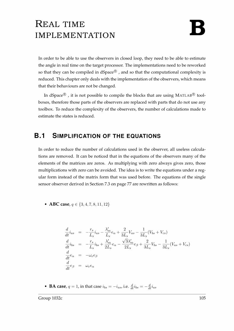
BREAL TIMEIMPLEMENTATION
In order to be able to use the observers in closed loop, they need to be able to estimate
the angle in real time on the target processor. The implementations need to be reworked
so that they can be compiled in dSpace R© , and so that the computational complexity is
reduced. This chapter only deals with the implementation of the observers, which means
that their behaviours are not be changed.
In dSpace R© , it is not possible to compile the blocks that are using MATLAB R© tool-
boxes, therefore those parts of the observers are replaced with parts that do not use any
toolbox. To reduce the complexity of the observers, the number of calculations made to
estimate the states is reduced.
B.1 SIMPLIFICATION OF THE EQUATIONS
In order to reduce the number of calculations used in the observer, all useless calcula-
tions are removed. It can be noticed that in the equations of the observers many of the
elements of the matrices are zeros. As multiplying with zero always gives zero, those
multiplications with zero can be avoided. The idea is to write the equations under a reg-
ular form instead of the matrix form that was used before. The equations of the single
sensor observer derived in Section 7.3 on page 77 are rewritten as follows:
• ABC case, q ∈ 3, 4, 7, 8, 11, 12
d
dtias = − rs
Lsias −
λ′mLs
eα +2
3LsVas −
13Ls
(Vbs + Vcs)
d
dtibs = − rs
Lsibs +
λ′m2Ls
eα −√
3λ′m2Ls
eβ +2
3LsVbs −
13Ls
(Vas + Vcs)
d
dteα = −ωeeβ
d
dteβ = ωeeα
• BA case, q = 1, in that case ibs = −ias, i.e. ddt ibs = − d
dt ias
Group 1032c 105

B.1. SIMPLIFICATION OF THE EQUATIONS
d
dtias = − rs
Lsias −
3λ′m4Ls
eα +√
3λ′m4Ls
eβ +1
2LsVas −
12Ls
Vbs + k6(ias +iccDin
)
d
dtibs = − d
dtias
d
dteα = −ωeeα + k8(ias +
iccDin
)
d
dteβ = ωeeβ + k9(ias +
iccDin
)
• AB case, q = 2, as for the BA case, ddt ibs = − d
dt ias
d
dtias = − rs
Lsias −
3λ′m4Ls
eα +√
3λ′m4Ls
eβ +1
2LsVas −
12Ls
Vbs + k6(ias −iccDin
)
d
dtibs = − d
dtias
d
dteα = −ωeeα + k8(ias −
iccDin
)
d
dteβ = ωeeβ + k9(ias −
iccDin
)
• CA case, q = 5
d
dtias = − rs
Lsias −
3λ′m4Ls
eα −√
3λ′m4Ls
eβ +1
2LsVas −
12Ls
Vcs + k10(ias +iccDin
)
d
dtibs = 0
d
dteα = −ωeeα + k11(ias +
iccDin
)
d
dteβ = ωeeβ + k12(ias +
iccDin
)
• AC case, q = 6
d
dtias = − rs
Lsias −
3λ′m4Ls
eα −√
3λ′m4Ls
eβ +1
2LsVas −
12Ls
Vcs + k10(ias −iccDin
)
d
dtibs = 0
d
dteα = −ωeeα + k11(ias −
iccDin
)
d
dteβ = ωeeβ + k12(ias −
iccDin
)
106 Aalborg University, Spring 2007
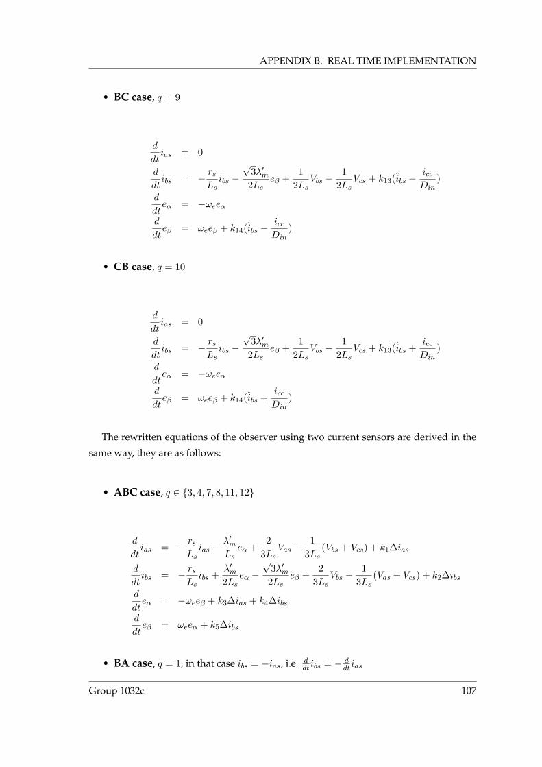
APPENDIX B. REAL TIME IMPLEMENTATION
• BC case, q = 9
d
dtias = 0
d
dtibs = − rs
Lsibs −
√3λ′m2Ls
eβ +1
2LsVbs −
12Ls
Vcs + k13(ibs −iccDin
)
d
dteα = −ωeeα
d
dteβ = ωeeβ + k14(ibs −
iccDin
)
• CB case, q = 10
d
dtias = 0
d
dtibs = − rs
Lsibs −
√3λ′m2Ls
eβ +1
2LsVbs −
12Ls
Vcs + k13(ibs +iccDin
)
d
dteα = −ωeeα
d
dteβ = ωeeβ + k14(ibs +
iccDin
)
The rewritten equations of the observer using two current sensors are derived in the
same way, they are as follows:
• ABC case, q ∈ 3, 4, 7, 8, 11, 12
d
dtias = − rs
Lsias −
λ′mLs
eα +2
3LsVas −
13Ls
(Vbs + Vcs) + k1∆ias
d
dtibs = − rs
Lsibs +
λ′m2Ls
eα −√
3λ′m2Ls
eβ +2
3LsVbs −
13Ls
(Vas + Vcs) + k2∆ibs
d
dteα = −ωeeβ + k3∆ias + k4∆ibs
d
dteβ = ωeeα + k5∆ibs
• BA case, q = 1, in that case ibs = −ias, i.e. ddt ibs = − d
dt ias
Group 1032c 107

B.1. SIMPLIFICATION OF THE EQUATIONS
d
dtias = − rs
Lsias −
3λ′m4Ls
eα +√
3λ′m4Ls
eβ +1
2LsVas −
12Ls
Vbs + k6∆ias
d
dtibs = − d
dtias
d
dteα = −ωeeα + k8∆ias
d
dteβ = ωeeβ + k9∆ias
• AB case, q = 2, as for the BA case, ddt ibs = − d
dt ias
d
dtias = − rs
Lsias −
3λ′m4Ls
eα +√
3λ′m4Ls
eβ +1
2LsVas −
12Ls
Vbs + k6∆ias
d
dtibs = − d
dtias
d
dteα = −ωeeα + k8∆ias
d
dteβ = ωeeβ + k9∆ias
• CA case, q = 5
d
dtias = − rs
Lsias −
3λ′m4Ls
eα −√
3λ′m4Ls
eβ +1
2LsVas −
12Ls
Vcs + k10∆ias
d
dtibs = 0
d
dteα = −ωeeα + k11∆ias
d
dteβ = ωeeβ + k12∆ias
• AC case, q = 6
d
dtias = − rs
Lsias −
3λ′m4Ls
eα −√
3λ′m4Ls
eβ +1
2LsVas −
12Ls
Vcs + k10∆ias
d
dtibs = 0
d
dteα = −ωeeα + k11∆ias
d
dteβ = ωeeβ + k12∆ias
108 Aalborg University, Spring 2007

APPENDIX B. REAL TIME IMPLEMENTATION
• BC case, q = 9
d
dtias = 0
d
dtibs = − rs
Lsibs −
√3λ′m2Ls
eβ +1
2LsVbs −
12Ls
Vcs + k13∆ibs
d
dteα = −ωeeα
d
dteβ = ωeeβ + k14∆ibs
• CB case, q = 10
d
dtias = 0
d
dtibs = − rs
Lsibs −
√3λ′m2Ls
eβ +1
2LsVbs −
12Ls
Vcs + k13∆ibs
d
dteα = −ωeeα
d
dteβ = ωeeβ + k14∆ibs
Under matrix form, the number of multiplications required is the same for all different
discrete states, as the sizes of the state vector, input vector, and estimation error vector
are constants. There are 4 states, 3 inputs, and 2 errors of estimation, this means that the
number of multiplications required is:
NbMultiplications = NbStates︸ ︷︷ ︸4
·(NbStates+NbInputs+NbErrors︸ ︷︷ ︸4+3+2=9
)
= 36
Table B.1 on the following page represents the number of multiplications that are re-
quired using the regular equations, i.e. without the matrix form. The table also shows
how the complexity of the calculation was reduced by rewriting the equations.
The table shows that rewriting the equations allowed to reduce the number of multi-
plications to 11 in the worst cases, meaning in ABC, AB, and BA cases. The computation
of the derivatives of the states has been reduced with 69% in those cases.
Group 1032c 109
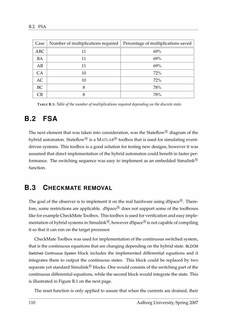
B.2. FSA
Case Number of multiplications required Percentage of multiplications saved
ABC 11 69%
BA 11 69%
AB 11 69%
CA 10 72%
AC 10 72%
BC 8 78%
CB 8 78%
TABLE B.1: Table of the number of multiplications required depending on the discrete state.
B.2 FSA
The next element that was taken into consideration, was the Stateflow R© diagram of the
hybrid automaton. Stateflow R© is a MATLAB R© toolbox that is used for simulating event-
driven systems. This toolbox is a good solution for testing new designs, however it was
assumed that direct implementation of the hybrid automaton could benefit in faster per-
formance. The switching sequence was easy to implement as an embedded Simulink R©
function.
B.3 CHECKMATE REMOVAL
The goal of the observer is to implement it on the real hardware using dSpace R©. There-
fore, some restrictions are applicable. dSpace R© does not support some of the toolboxes
like for example CheckMate Toolbox. This toolbox is used for verification and easy imple-
mentation of hybrid systems in Simulink R©, however dSpace R© is not capable of compiling
it so that it can run on the target processor.
CheckMate Toolbox was used for implementation of the continuous switched system,
that is the continuous equations that are changing depending on the hybrid state. BLDCM
Switched Continuous System block includes the implemented differential equations and it
integrates them to output the continuous states. This block could be replaced by two
separate yet standard Simulink R© blocks. One would consists of the switching part of the
continuous differential equations, while the second block would integrate the state. This
is illustrated in Figure B.1 on the next page.
The reset function is only applied to assure that when the currents are drained, their
110 Aalborg University, Spring 2007
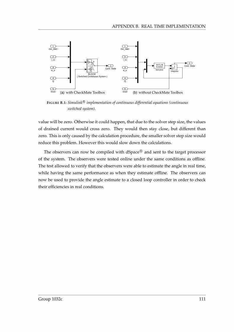
APPENDIX B. REAL TIME IMPLEMENTATION
1Cont. State
BLDCM ( Switched Continuous System )
5reset
4Q
3w_e
2i_cc
1Din_ABC
(a) with CheckMate Toolbox
1Cont. State
MATLABFunction
derivative
1s
Integrator
5reset
4Q
3w_e
2i_cc
1Din_ABC
(b) without CheckMate Toolbox
FIGURE B.1: Simulink R© implementation of continuous differential equations (continuous
switched system).
value will be zero. Otherwise it could happen, that due to the solver step size, the values
of drained current would cross zero. They would then stay close, but different than
zero. This is only caused by the calculation procedure, the smaller solver step size would
reduce this problem. However this would slow down the calculations.
The observers can now be compiled with dSpace R© and sent to the target processor
of the system. The observers were tested online under the same conditions as offline.
The test allowed to verify that the observers were able to estimate the angle in real time,
while having the same performance as when they estimate offline. The observers can
now be used to provide the angle estimate to a closed loop controller in order to check
their efficiencies in real conditions.
Group 1032c 111

This page is left intentionally blank

CRESULTS OF THE CLOSEDLOOP TESTS OF THEDOUBLE SENSOR OBSERVER
This appendix presents the results of the closed loop tests of the observer using phase
measurements to estimate the angle. The results are presented for different values of the
maximum angular velocity.
0 1 2 3 4 5 6 7 8 9 10−100
−50
−30
−15
0
15
30
50
100Error of estimation in the angle
Time [s]
Err
or [°
]
Error of estimationDifferent to 0 if in closed loop operation
FIGURE C.1: Error of estimation in the angle with maximum speed ωe = 215 [rad · s−1]
(ωr = 680 [rpm]).
Group 1032c 113
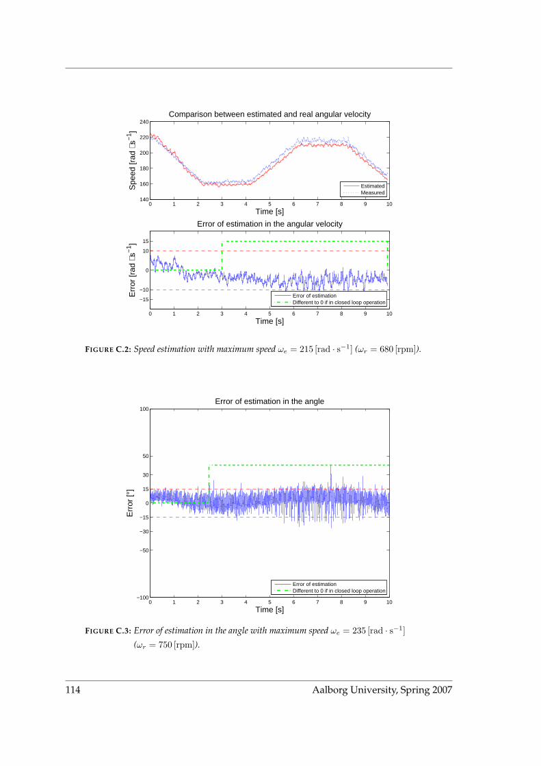
0 1 2 3 4 5 6 7 8 9 10140
160
180
200
220
240Comparison between estimated and real angular velocity
Time [s]
Spe
ed [r
ad ⋅
s−1 ]
EstimatedMeasured
0 1 2 3 4 5 6 7 8 9 10
−15
−10
0
10
15
Error of estimation in the angular velocity
Time [s]
Err
or [r
ad ⋅
s−1 ]
Error of estimationDifferent to 0 if in closed loop operation
FIGURE C.2: Speed estimation with maximum speed ωe = 215 [rad · s−1] (ωr = 680 [rpm]).
0 1 2 3 4 5 6 7 8 9 10−100
−50
−30
−15
0
15
30
50
100Error of estimation in the angle
Time [s]
Err
or [°
]
Error of estimationDifferent to 0 if in closed loop operation
FIGURE C.3: Error of estimation in the angle with maximum speed ωe = 235 [rad · s−1]
(ωr = 750 [rpm]).
114 Aalborg University, Spring 2007
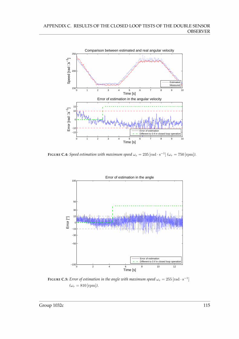
APPENDIX C. RESULTS OF THE CLOSED LOOP TESTS OF THE DOUBLE SENSOROBSERVER
0 1 2 3 4 5 6 7 8 9 10150
200
250Comparison between estimated and real angular velocity
Time [s]
Spe
ed [r
ad ⋅
s−1 ]
EstimatedMeasured
0 1 2 3 4 5 6 7 8 9 10
−15
−10
0
10
15
Error of estimation in the angular velocity
Time [s]
Err
or [r
ad ⋅
s−1 ]
Error of estimationDifferent to 0 if in closed loop operation
FIGURE C.4: Speed estimation with maximum speed ωe = 235 [rad · s−1] (ωr = 750 [rpm]).
0 2 4 6 8 10 12−100
−50
−30
−15
0
15
30
50
100Error of estimation in the angle
Time [s]
Err
or [°
]
Error of estimationDifferent to 0 if in closed loop operation
FIGURE C.5: Error of estimation in the angle with maximum speed ωe = 255 [rad · s−1]
(ωr = 810 [rpm]).
Group 1032c 115
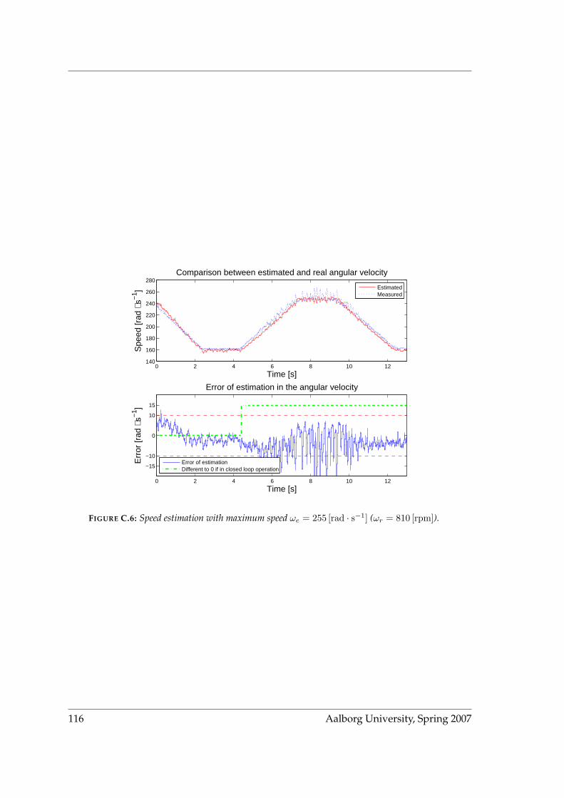
0 2 4 6 8 10 12140
160
180
200
220
240
260
280Comparison between estimated and real angular velocity
Time [s]
Spe
ed [r
ad ⋅
s−1 ]
EstimatedMeasured
0 2 4 6 8 10 12
−15
−10
0
10
15
Error of estimation in the angular velocity
Time [s]
Err
or [r
ad ⋅
s−1 ]
Error of estimationDifferent to 0 if in closed loop operation
FIGURE C.6: Speed estimation with maximum speed ωe = 255 [rad · s−1] (ωr = 810 [rpm]).
116 Aalborg University, Spring 2007

NOMENCLATURE
Bm Damping coefficient of the motor
Din Input duty cycle to the inverter
eα, eβ States that correspond to the back-EMF
eθ Error between the electrical angle calculated by the observer, θe, and the
measured angle, θe
iabcs Vector of currents through the phases
icc Supply current to the inverter
∆i Difference between estimated and measured currents
i Estimated current vector: i =[ias ibs
]Tixs Stator current in phase x
J Moment of inertia of the rotating part, i.e. rotor and load
qK Proportional gain matrix in the observer in location q
λ number of offspring in population
λ′m Magnitude of the fundamental component of the back-EMF
Ls Equivalent inductance of a phase
µ number of parents in population
ωe Estimated electrical angular velocity
Q Cost function
rs Ohmic resistance of a phase
Te Torque produced by the motor
θe Estimated electrical angle of the rotor
θe Electrical angle
θr Mechanical angle
Group 1032c 117

TL Torque produced by the load
TPWM Period of the PWM signal, TPWM = 6.25 · 10−5 [s]
Ts Sampling period of the system, Ts = 6.25 · 10−5 [s]
Vabcs Vector of input voltages
ϕ Mutation coefficient
Vcc Supply voltage of the current inverter
Vn Neutral node potential
Vxs Input Potential to phase x in stator reference frame
xo Offspring individual
ωe, ωr Electrical and mechanical angular velocity
xp Parent individual
Zp Number of magnetic pole pairs
ACRONYMS
ANN Artificial Neural Networks
BLDCM Brushless DC Motor
EA Evolutionary Algorithm
EC Evolutionary Computation
EMF ElectroMotive Force
DE Differential Evolution
FSA Finite State Automaton
NSS Nonlinear Simplex Search
PM Permanent Magnet
PPT PWM-PWM-Tristate
118 Aalborg University, Spring 2007

PSO Particle Swarm Optimization
PWM Pulse Width Modulation
RWC Random Weight Change
SI Swarm Intelligence
SUS Stochastic Universal Sampling
Group 1032c 119