Embed Size (px)
Citation preview

Master Physician Scheduling Problem1
Aldy Gunawan and Hoong Chuin Lau
School of Information Systems, Singapore Management University, Singapore
Abstract
We study a real-world problem arising from the operations of a hospital service provider,
which we term the master physician scheduling problem. It is a planning problem of
assigning physicians’ full range of day-to-day duties (including surgery, clinics, scopes,
calls, administration) to the defined time slots/shifts over a time horizon, incorporating a
large number of constraints and complex physician preferences. The goals are to satisfy as
many physicians’ preferences and duty requirements as possible while ensuring optimum
usage of available resources. We propose mathematical programming models that
represent different variants of this problem. The models were tested on a real case from
the Surgery Department of a local government hospital, as well as on randomly generated
problem instances. The computational results are reported together with analysis on the
optimal solutions obtained. For large-scale instances that could not be solved by the
exact method, we propose a heuristic algorithm to generate good solutions.
Keywords: scheduling, optimization, health service, master physician scheduling and
rostering problem, mathematical programming, preferences.
Introduction
There has been increased interest in hospital operations management in terms of
optimized scheduling and allocation of employees (e.g. physicians, nurses and
administrators). One problem is to design a physician schedule which takes a large
number of constraints and physician preferences into account.
A physician schedule is an assignment of physicians to perform different duties in
the hospital timetable. Unlike nurse rostering which has been extensively studied in the
literature (e.g. Ernst et al, 2004a; Glass and Knight, 2009; Petrovic and Vanden Berghe,
2008), in physician scheduling, maximizing satisfaction matters primarily, as physician
retention is the most critical issue faced by hospital administrations (Carter and Lapierre,
2001). In addition, while nurse schedules must adhere to collective union agreements,
physician schedules are more flexible and driven by personal preferences. Carter and
Lapierre (2001) also provides the fundamental differences between physicians and nurses
1 Pre-print for A. Gunawan and H. C. Lau. Master Physician Scheduling Problem. Journal of the
Operational Research Society, 64 (3), 410-425, 2013.

2
scheduling problems. In general, scheduling physicians requires satisfying a large number
of conflicting constraints and preferences.
To our knowledge, research on physician scheduling has focused primarily on a
single type of duty, such as the emergency room (e.g. Beaulieu et al., 2000; Carter and
Lapierre, 2001; Gendreau et al., 2007; Puente et al., 2009), the operating room (e.g. Testi
et al., 2007; Burke and Riise, 2008; Roland et al., 2010; Vanberkel et al., 2011), the
physiotherapy and rehabilitation services (Ogulata et al., 2008). In this paper, we consider
the problem of generating a master schedule for the physicians within a hospital service
by taking a full range of day-to-day duties/activities of the physicians (including surgery,
clinics, scopes, calls, administration) into consideration. Our problem, termed the Master
Physician Scheduling Problem, involves the assignment of physician activities to the
time slots over a time horizon, incorporating rostering and resource constraints together
with complex physician preferences. The goals are to satisfy as many physicians’
preferences and duty requirements as possible.
The major contributions/highlights of this paper are as follows:
(1) We take a physician-centric approach to solving this problem, since physician
retention is the most critical issue faced by hospital administrations worldwide.
(2) Using mathematical models, we provide a comprehensive empirical understanding of
the tradeoff of constraints and preferences against resource capacities.
The paper is organized as follows. We first provide a review of the literature, before
presenting a detailed description of the problem. We then address variants of the problem
each with a single objective and provide mathematical programming models. We also
extend and formulate the problem as a bi-objective mathematical programming model.
For this Weighted-Sum model, the varying values of weights are calculated by linear
interpolation between solutions in order to obtain a set of Pareto-optimal solutions. Our
developed models are tested on a real case from the Surgery Department of a large local
government hospital, as well as on randomly generated problem instances. Computational
results are reported together with our analysis. We also propose a heuristic algorithm to
solve the single objective problem that could not be solved optimally within reasonable
time by the exact method, and provide computational results. Finally, we provide
concluding perspectives and directions for future research.
Literature Review
Personnel scheduling and rostering is becoming a critical concern in service organizations
such as emergency services, higher education systems, health care systems, hospitality,
and transportation systems. Scheduling in service organizations is different from that of
manufacturing systems (Aggarwal, 1982). Some of the major differences are that the

3
output of service systems cannot be placed into inventory, the customer receives the
service directly from the server and so on. The primary objective of the manufacturing
system is to minimize the total cost, while the service systems deal with conflicting
objectives, such as minimizing total cost and maximizing staff satisfaction as regards their
schedules.
A number of reviews in personnel scheduling and rostering research have appeared
in Aggarwal (1982), Burke et al. (2004) and Ernst et al. (2004b). A categorization of
comprehensive and representative solution techniques employed for different rostering
problems are found in Ernst et al. (2004b). A number of approaches including artificial
intelligence approaches, constraint programming, metaheuristics, and mathematical
programming approaches have been used for solving the specific problems.
Beaulieu et al. (2000) proposed a mixed 0-1 programming formulation of the
physician scheduling problem. They claimed that their work was the first to present a
mathematical programming approach for scheduling physicians in the emergency room in
a major hospital of the Montréal region. The basic rules applied at the hospital are
distinguished into two categories: compulsory (or hard) and flexible (or soft) rules.
However, this classification depends on the preferences of the hospital and on the
physician’s flexibility. The constraints are partitioned into four different categories
according to the types of rules to which they correspond: compulsory constraints,
ergonomic constraints, distribution constraints, and goal constraints. The objective
function is to minimize all deviations of the goal constraints. The problem was then
solved by a heuristic approach based on a partial branch-and-bound. The schedules
produced were compared with those generated by a human expert in terms of the
computation time, the effort required and the solution quality.
Gendreau et al. (2007) presented several generic forms of the constraints encountered
in six different hospitals in the Montréal area (Canada) as well as several possible solution
techniques for solving the problem. The constraints of the physician scheduling problem
can be classified into four categories: supply and demand constraints, workload
constraints, fairness constraints and ergonomic constraints. In this paper, we are
concerned about the physicians’ preferences instead of fairness constraints. Four solution
techniques that can be applied to the physician scheduling problem are categorized into
four different categories: mathematical programming, column generation, tabu search and
constraint programming.
A number of exact and heuristic algorithms for various scheduling problems
encountered in hospitals were also proposed by Beliën (2007). The first problem, namely
the trainee scheduling problem, is solved by branch-and-price algorithm (Beliën and
Demeulemeester, 2006). The second problem, the operating room scheduling problem, is
4
modelled as a number of mixed integer programming based heuristics and simulated
annealing algorithm (Beliën and Demeulemeester, 2007). These models consider
stochastic number of patients for each operating room block and a stochastic length of
stay for each operated patient. The main objective is to minimize the expected total bed
shortage.
Buzon and Lapierre (1999) applied tabu search to acyclic schedules. The cost of the
solution is the sum of the costs of all physician schedules where each cost represents the
sum of all penalties associated with the unsatisfied constraints. Constraint programming
has been applied to the nurse scheduling problem (Bard and Purnomo, 2005). This
solution technique can also be applied to the physician scheduling problem after some
minor modifications. Rousseau et al. (2002) and Bourdais et al. (2003) presented a
hybridization of a constraint programming model and search techniques with local search
as well as some ideas from genetic algorithms to the physician scheduling problem.
The physician and nurse scheduling problem are inherently multi-objective
optimization problem with conflicting objectives. (Burke et al., 2009) model these as soft
constraints. Some classical methods for handling multi-objective optimization problem
have been proposed in literature. One of the most commonly used method is goal
programming since it allows simultaneous solution of multiple objectives (Ogulata and
Erol, 2003; Topaloglu, 2006; White et al., 2006). Burke et al. (2009) presented a Pareto-
based optimization technique based on a simulated annealing algorithm to address nurse
scheduling problems in the real world.
Problem Definition
The problem addressed in this paper is to assign different physician duties (or activities)
to the defined time slots over a time horizon incorporating a large number of constraints
and complex physician preferences. For simplicity, we assume the time horizon to be one
working week (Mon-Fri), further partitioned into 5 days and 2 shifts (AM and PM). The
problem that we address is a real problem in the Surgery Department of a large
government hospital.
Physicians have a fixed set of duties to perform, and they may specify their
respective ideal schedule in terms of the duties they like to perform on their preferred
days and shifts, as well as shifts-off or days off. Taking these preferences together with
resource capacity and rostering constraints into consideration, our goal is to generate an
actual schedule. As shown in Figure 1 as example, the ideal schedules might not be fully
satisfied in the actual schedule. That may occur in two scenarios:
Some duties have to be scheduled on different shifts or days – which we term non-
ideal scheduled duties (e.g. Physician 2, Tuesday duties).

5
Some duties simply cannot be scheduled due to resource constraints – which we term
unscheduled duties (e.g. Physician 1, Friday PM duty).
Physician Physician
1 2 … |I| 1 2 … |I|
Monday AM Duty 1 - … Duty 3 Monday AM Duty 1 - … Duty 5
PM Duty 5 Duty 4 … Duty 1 PM Duty 5 Duty 4 … Duty 1
Tuesday AM - Duty 1 … Duty 5
Tuesday AM - Duty 5 … Duty 3
PM Duty |L| Duty 5 … Duty 2 PM Duty |L| Duty 1 … -
: : : : : : : :
: : : : : : : :
Friday AM Duty 4 - … Duty |L| Friday AM Duty 4 - … Duty |L|
PM Duty 1 Duty |L| … - PM - Duty |L| … -
Physicians’ Ideal Schedule Actual Schedule
Figure 1. Example of Master Physician Scheduling Problem
Although each hospital has its unique rostering requirements, the following
summarizes some common requirements treated in this paper:
No physician can perform more than one duty in any shift.
The number of resources (e.g. operating theatres, clinics) needed cannot exceed their
respective capacities at any time. For simplicity, we assume that each type of activity
does not share its resources with another type of activities – for example, operating
theatres and clinics are used to perform surgery and out-patient duties, respectively.
Ergonomic constraints: Some duties are regarded as heavy duties, such as surgery
and endoscopy duties. The following ergonomic constraints hold:
o If a physician is assigned to a heavy duty in the morning shift, then he cannot be
assigned to another type of heavy duty in the afternoon shift on the same day.
However, it is possible to assign the same type of heavy duties in consecutive
shifts on the same day.
o Similarly, a physician cannot also be assigned to another type of heavy duty in the
morning shift on a particular day if he has been assigned to a heavy duty in the
afternoon shift on the previous day.
Note that there are other ergonomic constraints (such as those presented by Gendreau
et al. (2007) on constraints related to night shift). In this paper, these constraints do
not apply as we consider only two different shifts (AM and PM). They may be added
without loss of generality to our proposed models.

6
The number of activities allocated to each physician cannot exceed his contractual
commitments, and do not conflict with his external commitments. In this paper, we
assume external commitments take the form of physicians’ request for shifts-off or
days-off, and hence no duty should be assigned to these requests.
We study different settings that may be instantiated from the problem. The basic
problem (known as Model I) is to minimize the total number of unscheduled duties in an
unconstrained setting (i.e. without any physician preferences or ergonomic constraints).
From this basic problem, we look into two constrained problem settings that respectively
handle physician preferences and ergonomic constraints. The first is the problem of
satisfying the physicians’ ideal schedule as far as possible (or maximizing the total
number of ideal scheduled duties) while not compromising on having the minimum
number of unscheduled duties. The second is the setting where physicians do not provide
their ideal schedule, but instead ergonomic constraints are employed across all physicians
in minimizing the total number of unscheduled duties. Both problem settings are
formulated as Models IIa and IIb, respectively. Finally, we also consider the problem that
optimizes physician ideal schedules on one hand, and on the other, improves the quality of
duty transition on non-ideal scheduled slots through ergonomic constraints.
Mathematical Programming Models
In this section, following a presentation of the notations used in this paper, we will
provide the mathematical programming formulation of the basic model (Model I), single
objective models (Models IIa and IIb) and finally the bi-objective model (Model III).
Basic notations:
I = Set of physicians, I,,,i 21
J = Set of days, J,,,j 21
K = Set of shifts per day, K,,,k 21
L = Set of duties, L,,,l 21
HL = {l L : l = heavy duty}
PRA = {(i, j, k) I × J × K : (i, j, k) = physician i requests not being assigned on day j
shift k}
Data parameters:
lR = number of resources required to perform duty l (lL)
jklC = number of resources available for duty l on day j shift k (jJ, kK, lL)
(i.e. resource capacity)
ilA = number of duty l requested by physician i in a weekly schedule (i I, lL)
ijklF = 1 if physician i requests duty l on day j shift k, 0 otherwise
Decision and auxiliary variables:

7
ijklX = 1 if physician i is assigned to duty l on day j shift k, 0 otherwise
iU = number of unscheduled duties of physician i
iN = number of non-ideal scheduled duties of physician i
iS = number of ideal scheduled duties of physician i
The unconstrained problem (Model I) is one of minimizing the number of unscheduled
duties subject to resource capacity constraints. It is formulated as follows:
[Model I]
Minimize Ii iUZ (1)
Subject to:
jklIi ijkll CXR LlK,kJ,j (2)
ilJj Kk ijkl AX LlI,i (3)
1
Ll ijklX KkJ,jI,i (4)
Ll ijklX 0 PRAkj,i, (5)
Ll Jj Kk Ll ijklili XAU Ii (6)
1,0ijklX LlK,kJ,jI,i (7)
ZU i Ii (8)
Constraint (1) is the total number of unscheduled duties that needs to be minimized.
Constraint (2) is the resource capacity constraint (total number of resources required does
not exceed total number of available resources per shift)2. Therefore, lR is set to zero for
activities without limited number of resources available. Through constraint (3), the
number of duties allocated to each physician cannot exceed his contractual commitments.
Constraint (4) ensures that each physician cannot be assigned more than one duty in any
shift, while constraint (5) ensures that no duty would be assigned to a physician during
any shifts-off or days-off requested. Equation (6) defines the number of unscheduled
duties (which is to be minimized). Constraint (7) imposes the 0-1 restrictions for the
decision variables Xijkl, while constraint (8) is the nonnegative integrality constraint for the
decision variables Ui. Model I computes the minimum number of unscheduled duties with
only resource capacity constraints. It therefore provides the lower bound on the number of
unscheduled duties as we constrain the problem further in subsequent models below.
Model IIa extends the base model by considering the physicians’ ideal schedule. Let
*iU denote the optimal solution containing the number of unscheduled duties for physician
i obtained by Model I. In order to keep to the number of unscheduled duties for each
physician to this value, we impose this value as an upper bound (see constraint (10)).
Model IIa seeks to then maximize the total number of ideal scheduled duties. The total
2In (Gunawan and Lau, 2009), we defined an additional notation Lc to represent a set of duties with limited
number of resources available. In this journal version, L is used to simplify notations.
8
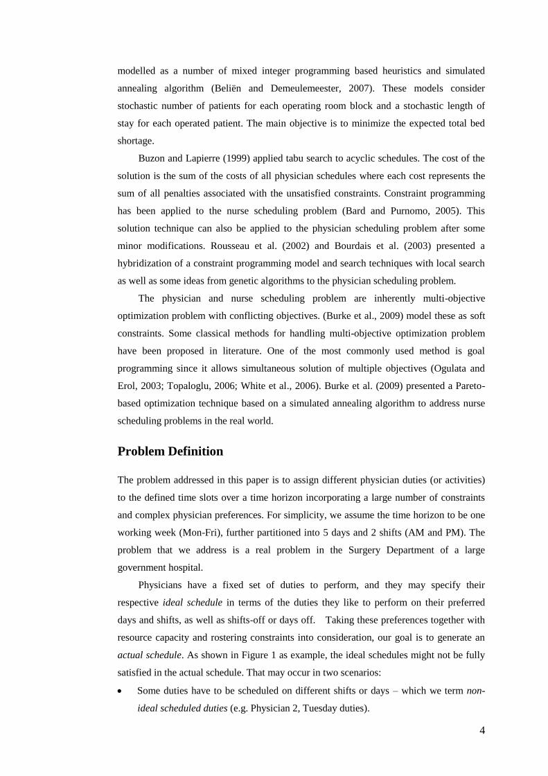
numbers of unscheduled, ideal and non-ideal duties for each physician are calculated by
equations (6), (11)–(12). The rest of the constraints are identical to those of Model I.
[Model IIa]
Maximize
Ii Jj Kk Ll ijklijkl FXZ (9)
Subject to:
(2) - (8) *ii UU Ii (10)
Jj Kk Ll ijklijkli FXS
Ii (11)
Ii iiili USAN
Ii (12)
ZS,N,U iii Ii (13)
We next consider another problem setting where constraints are imposed on duty
transition, which is formulated as Model IIb. Here, we assume that duties are classified
into two different groups: heavy and light duties. A physician assigned to a heavy duty in
a particular shift cannot be assigned to a different heavy duty in the next shift on the same
day, as represented by constraint (15); nor a different heavy duty in the first shift on the
next day (constraint (16)). However, physicians can perform the same heavy duties in
consecutive shifts. Such ergonomic constraints apparently reduce the fatigue factor and
improve physician productivity and hence quality of service.
[Model IIb]
Minimize Ii iUZ (14)
Subject to:
(2) – (8)
11 2lkij1ijkl XX 212112,1 llLl&l,K,,kJ,jI,i H (15)
121
11 ljilKijXX 212112,1 llLl&l,J,,jI,i H (16)
Observation: Model I is a basic model without ergonomic constraints, while Model IIb is
an extended model with ergonomic constraints. Hence, the optimal number of
unscheduled duties obtained by Model IIb is greater than or equal to that of Model I.
In Model III, we combine the two problem settings (i.e. Model IIa and IIb) presented
previously. More precisely, we are concerned with the bi-objective problem of
maximizing the number of ideal scheduled duties and minimizing the number of
unscheduled duties under ergonomic constraints. Note that in Model IIa, we assume that
non-ideal scheduled duties can be allocated at any time period without considering
ergonomic constraints. In this combined problem, we improve the quality of the duty

9
transition of each physician by imposing ergonomic constraints on non-ideal scheduled
duties.
In the following, we propose an approach to solve the problem, which is based on
weighted-sum method that obtains Pareto-optimal solutions. Two additional sets of
decision variables are defined as follows:
ijklX = 1 if physician i is assigned to duty l on day j shift k with respect to the ideal
schedule, 0 otherwise
ijklY = 1 if physician i is assigned to duty l on day j shift k with respect to ergonomic
constraints, 0 otherwise
A classical multi-objective weighted-sum method combines the two objectives into a
single objective by multiplying each objective with a user-defined weight. This weighted-
sum model is then embedded within a proposed algorithm to obtain a set of Pareto-
optimal solutions (Figure 2).
[Model III]
Minimize Ii iIii )U(W)S(WZ 21 (17)
Subject to:
jklIi ijklijkll CYX(R )ˆˆ LlK,kJ,j (18)
1ˆˆ ijklijkl YX LlK,kJ,jI,i (19)
ilJj ijklKk ijkl A)YX( ˆˆ LlI,i (20)
1ˆˆ Ll ijklijkl )YX( KkJ,jI,i (21)
Ll ijklijkl )YX( 0ˆˆ PRAkj,i, (22)
ijklijkl FX ˆ LlK,kJ,jI,i (23)
Jj Kk Ll ijklijklLl ili YXAU )ˆˆ( Ii (24)
Jj Kk Ll ijkli XS ˆ Ii (25)
Jj Kk Ll ijkli YN ˆ Ii (26)
1ˆˆˆ221 11 lkijlkijijkl YXY
212112,1 llLl&l,K,,kJ,jI,i H (27)
1ˆˆˆ221
1111 ljiljilKij YXY
212112,1 llLl&l,J,,jI,i H (28)
1ˆˆˆ221
11 lijlijlKij YXY
2121 llLl&lJ,jI,i H
(29)
1ˆˆˆ221 111 lKjilKjilij YXY
21213,2 llLl&l,J,...,jI,i H (30)
1,0ˆ,ˆ ijklijkl YX LlK,kJ,jI,i (31)
ZS,NU iii , Ii (32)
Note that in Model III above, maximizing the total number of ideal scheduled duties
is equivalent to minimizing the function given by (-1) × total number of ideal scheduled
duties. In this model, the objective function and some of constraints are identical to those

10
of Model IIa. Constraint (21) ensures that a duty is scheduled as either an ideal or a non-
ideal duty. The details of ergonomic constraints are represented by equations (27) – (30).
Finally, constraint (31) imposes the 0-1 restrictions for the decision variables ijklX and
ijklY while constraint (32) is the nonnegative integrality constraint for the decision
variables iU , iN and iS .
The advantage of the weighted-sum method is that it guarantees finding Pareto-
optimal solutions for convex optimization problems, which can be inferred from Deb
(2003) Theorem 3.1.1:
Corollary: The solution to Model III is not Pareto-optimal iff either W1 or W2 is set to
zero.
We efficiently generate a set of Pareto-optimal solutions for Model III by using the
following algorithm. We first generate k (constant) number of solutions with different
values of W1 uniformly distributed between [0, 1]. Since not all Pareto-optimal solutions
may be discovered by the initial set of weights, we introduce an adaptive exploration on
the neighbourhood of weights using linear interpolation, i.e. we examine two different
Pareto-optimal solutions to derive weights for obtaining other possible optimal solutions.
The details of the algorithm for using Model III to obtain Pareto-optimal solutions are
presented in Figure 2.
(1) Set W1 = 1
(2) Repeat
(3) Set W2 = 1 - W1
(4) Solve Model III
(5) W1 = W1 – 0.1
(6) Until W1 < 0
(7) For all solutions generated by the above, let S denote the subset of Pareto-optimal solutions
(8) For a pre-set number of iterations do the following
(9) Let S1 and S2 ( S) with the lowest and the second lowest total number of unscheduled duties,
respectively
(10) Set W′1 = W1 of solution S1 and W′2 = W2 of solution S1
(11) Set W′′1 = W1 of solution S2 and W′′2 = W2 of solution S2
(12) Calculate new weights, denoted as W*1 and W*2, as follows:
W*1 = (W′1 + W′′1)/2
W*2 = 1 - W*1
(13) Solve Model III with W1 = W*1 and W2 = W*2
(14) If the solution obtained is a new Pareto-optimal solution then
(15) Update S
(16) Else if the solution obtained and S1 are the same then
(17) Set the solution obtained as S1 and Update S
(18) Else if the solution obtained and S2 are the same then
(19) Set the solution obtained as S2 and Update S
Figure 2. Algorithm to obtain Pareto-optimal solutions
Computational Results

11
In this section, we report a comprehensive suite of experimental results which aims to
provide computational perspectives on one hand, and insights to hospital administrators
on the other. All models were solved by the CPLEX 10.0 solver engine.
Experimental Setup
First we discuss problem instance generation. 6 sets of random instances (Random 1 to 6)
were generated with varying values of the following parameters : total percentage of
heavy duties assigned to physicians (last column of Table 1) and number of resources
available in every shift (Table 2). This is to enable sensitivity analysis, which will be
described in more detail after the results reported (Figure 3). Other parameters, such as
number of heavy duties and number of duties with limited resource capacity, are set to a
constant. In addition to random instances, we also provide a real case study provided by
the Surgery Department of a large local government hospital and several other quasi-
random instances (Random 7, 8 and 9) which have similar characteristics to the real case,
to help understand the nature of the real case study. Table 1 summarizes the
characteristics of each problem set. In order to generate sufficient hard problem instances
for the purpose of sensitivity analysis, the resource capacity level has to be carefully set,
and interested reader can refer to Gunawan and Lau (2009).
Table 1. Characteristics of Problem Instances
Problem Set Number
of
physicians
Number of shifts per
day
Number
of days
Number
of duties
Number of heavy
duties
Number of
duties with
limited capacity
Total
percentage
of heavy duties*
Case study 15 2 5 9 3 3 73%
Random 1 20 2 5 7 3 3 20%
Random 2 20 2 5 7 3 3 30% Random 3 20 2 5 7 3 3 40%
Random 4 20 2 5 7 3 3 50%
Random 5 20 2 5 7 3 3 60% Random 6 20 2 5 7 3 3 70%
Random 7 15 2 5 9 3 3 75%
Random 8 16 2 5 9 3 3 75% Random 9 50 2 5 7 5 3 69%
%|K||J||I|/A* Ii Ll ilH 100
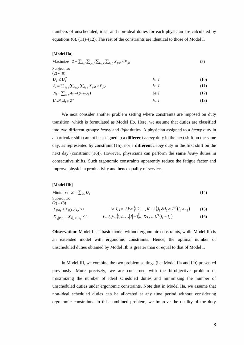
As an illustration, Table 2 presents three columns that give the varying values of Cjkl
for different duties defined in the instances of the Random 1 problem sets. The total
number of resources required for Duty 1, Duty 2 and Duty 3 are 15, 28 and 22,
respectively. Here, Duty 2 is the duty with the highest number of resources required and
hence the value of Cjkl for Duty 2 is set to
52
282 and decreases by one unit until it is
equal to 152
28
. For Duty 1 and Duty 3, we set the initial values of Cjkl to 1
52
15
12
and 152
22
, respectively and varying the values according to the description given
above. For instance, for Duty 1, by varying the values for Cjkl, there are 7 different
problem instances generated.
Table 2. Examples of varying values of Cjkl (Random 1 instances)
Problem Set Instances L
Duty 1 Duty 2 Duty 3
Random 1
15 28 22
Random 1a 3 6 4
Random 1b 3 5 4
Random 1c 3 4 4
Random 1d 3 3 4
Random 1e 3 3 3
Random 1f 2 3 3
Random 1g 1 2 2
In the following, we report a suite of computational results and analysis obtained
from our mathematical models described above. Our mathematical models were
implemented using CPLEX 10.0 and executed on a Intel (R) Core (TM)2 Duo CPU
2.33GHz with 1.96GB RAM that runs Microsoft Windows XP.
Results from Model I and IIa
First, results obtained from Model I for Random 1 and Random 2 problems are shown in
Table 3. It is interesting to observe a two-point phase transition in the minimum number
of unscheduled duties (column 2) with changing values of Cjkl. It remains unchanged over
a sufficiently large range of values. As the value of Cjkl of the duty with the highest
requirement tends to
JK
AR Ii ill , the number of unscheduled duties starts to increase.
For example, as we decrease the Cjkl’s value for Duty 2 from 6 to 4 for Random 1
instances, the number of unscheduled duties remains zero, but when this value reaches 3,
the number of unscheduled duties increases to 4. Then, when the number of resources
available is set to 1
JK
AR Ii ill for each activity Ll , the number of unscheduled
duties increases drastically from 5 to 10 unscheduled duties. The same behavior was also
observed for the other problem sets listed in Table 1.
From Table 3 again, we observe that the number of unscheduled duties is very low in
comparison to the number of scheduled duties. The percentage of unscheduled duties is on
average less than 3% for Random 1 and Random 2 instances. Similar observations are
made for other random problem sets. These results demonstrate the effectiveness of the
optimization model on random hard instances. It is interesting to see these results in the
light of the real-world case study problem instance where the percentage of unscheduled

13
duties obtained is around 4.7%. This gives evidence to the hospital management that their
resource capacity has reached a critical threshold as typified by problem instances 1g and
2i, and consequently will experience a drastic reduction of performance if resources
cannot come up to par with physician duties.
Table 3. Summary of results for Models I and IIa
Problem
Instances
Number of
unscheduled
duties
Number of scheduled duties Percentage of
unscheduled
duties (%)
Percentage of scheduled duties
(%)
Ideal Non-ideal Ideal Non-ideal
Case study 7 139 4 4.7 92.6 2.7
Random 1a 0 196 4 0 98 2
Random 1b 0 192 8 0 96 4
Random 1c 0 192 8 0 96 4
Random 1d 4 186 10 2 93 5
Random 1e 5 179 16 2.5 89.5 8
Random 1f 5 178 17 2.5 89 8.5
Random 1g 10 173 17 5 86.5 8.5
Random 2a 0 196 4 0 98 2 Random 2b 0 196 4 0 98 2
Random 2c 0 196 4 0 98 2
Random 2d 0 194 6 0 97 3
Random 2e 0 194 6 0 97 3
Random 2f 3 184 13 1.5 92 6.5
Random 2g 3 184 13 1.5 92 6.5
Random 2h 3 183 14 1.5 91.5 7
Random 2i 10 176 14 5 88 7
Table 3 also presents results on the extent of the satisfiability of ideal schedule in the
actual schedule, obtained from running Model IIa. These results are illustrated in Figures
3(a) and 3(b). Note that the left axes in both figures measure the percentage of ideal, non-
ideal scheduled and unscheduled; and the resource availability/requirement gap %Gap
respectively. The resource availability/requirement gap is defined
as %100
Ii Ll ill
Jj Kk Ll Ii Ll illjkl
AR
ARCLK% Gap . It represents a resource
buffer, i.e. the proportion of total resource availability that exceeds the sum of resource
requirement requested.
(a) (b)
Figure 3. Parameter analysis of Random 1 Problem Set

14
From Figure 3(a), we can infer that in order to ensure zero unscheduled duties
(which is often a hard constraint, since doctor duties should not be unfulfilled), the total
number of available resources for each activity Ll must be above the threshold
1
JK
ARIi ill (see instances 1a, 1b and 1c). From Figure 3(b), we can also infer that
when the %Gap is decreased below 23%, the percentage of unscheduled duties will be
doubled (see instances 1f vs 1g, also 2h vs 2i). Similar observations have been made for
the rest of the problem instances. From the hospital administration standpoint, the latter
result shows the critical resource availability threshold below which the degradation of
service performance will be keenly felt.
Next, the result of the case study problem instance is compared with that of the
actual allocation generated manually by the hospital, as summarized in Table 4. Although
the number of unscheduled duties via manual allocation is smaller than the results
obtained by Model IIa, the number of non-ideal scheduled duties is significantly higher
than that of the model solution. Note also that the manual allocation is strictly speaking
not feasible, since two physicians had to cancel their days-off or shifts-off to perform their
duties. This manual plan is therefore very undesirable since physicians might have
external commitments that cannot be delayed or cancelled. Suppose that the two
physicians are unwilling to fulfill these duties on their days-off or shifts-off, the number
of unscheduled duties would be equal to the solution obtained by our proposed approach.
We conclude that our proposed approach performs better than the manual allocation.
Table 4. Comparison between the manual allocation and model solution on a real case
Manual allocation Optimal solution
Number of unscheduled duties 5 7
Number of non-ideal scheduled duties 10 4
Number of physicians assigned duties during days-off or shifts-off 2 0
Results from Model IIb
Table 5 presents results obtained by running Model IIb against our problem instances.
We observe that Random 6 (where the percentage of heavy duties reaches 70%) and
Random 9 problem sets could not be solved to optimality within the computation time
limit of 6 hours. As such, we only report the best known solutions that could be obtained
for these problem instances.
Using Model IIb, we perform sensitivity analysis on the impact of ergonomic
constraints on resource utilization, which is of great interest to the hospital administrator.
Particularly, for solutions with non-zero unscheduled duties (see instances 1d-1g, …, 5j-
5m, etc on Table 5), the question is the resource level actually needed to bring the number
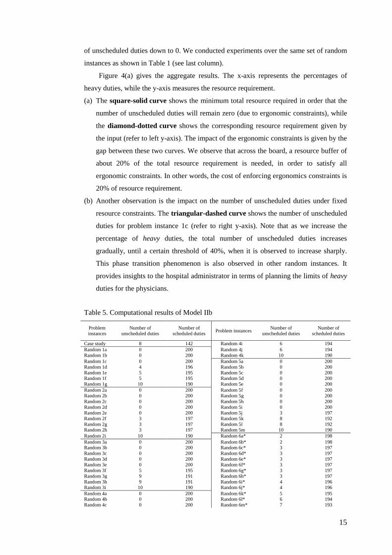
15
of unscheduled duties down to 0. We conducted experiments over the same set of random
instances as shown in Table 1 (see last column).
Figure 4(a) gives the aggregate results. The x-axis represents the percentages of
heavy duties, while the y-axis measures the resource requirement.
(a) The square-solid curve shows the minimum total resource required in order that the
number of unscheduled duties will remain zero (due to ergonomic constraints), while
the diamond-dotted curve shows the corresponding resource requirement given by
the input (refer to left y-axis). The impact of the ergonomic constraints is given by the
gap between these two curves. We observe that across the board, a resource buffer of
about 20% of the total resource requirement is needed, in order to satisfy all
ergonomic constraints. In other words, the cost of enforcing ergonomics constraints is
20% of resource requirement.
(b) Another observation is the impact on the number of unscheduled duties under fixed
resource constraints. The triangular-dashed curve shows the number of unscheduled
duties for problem instance 1c (refer to right y-axis). Note that as we increase the
percentage of heavy duties, the total number of unscheduled duties increases
gradually, until a certain threshold of 40%, when it is observed to increase sharply.
This phase transition phenomenon is also observed in other random instances. It
provides insights to the hospital administrator in terms of planning the limits of heavy
duties for the physicians.
Table 5. Computational results of Model IIb
Problem instances
Number of unscheduled duties
Number of scheduled duties
Problem instances Number of
unscheduled duties Number of
scheduled duties
Case study 8 142 Random 4i 6 194
Random 1a 0 200 Random 4j 6 194
Random 1b 0 200 Random 4k 10 190
Random 1c 0 200 Random 5a 0 200
Random 1d 4 196 Random 5b 0 200
Random 1e 5 195 Random 5c 0 200 Random 1f 5 195 Random 5d 0 200
Random 1g 10 190 Random 5e 0 200
Random 2a 0 200 Random 5f 0 200
Random 2b 0 200 Random 5g 0 200
Random 2c 0 200 Random 5h 0 200
Random 2d 0 200 Random 5i 0 200
Random 2e 0 200 Random 5j 3 197
Random 2f 3 197 Random 5k 8 192
Random 2g 3 197 Random 5l 8 192 Random 2h 3 197 Random 5m 10 190
Random 2i 10 190 Random 6a* 2 198
Random 3a 0 200 Random 6b* 2 198 Random 3b 0 200 Random 6c* 3 197
Random 3c 0 200 Random 6d* 3 197
Random 3d 0 200 Random 6e* 3 197
Random 3e 0 200 Random 6f* 3 197
Random 3f 5 195 Random 6g* 3 197
Random 3g 9 191 Random 6h* 3 197
Random 3h 9 191 Random 6i* 4 196 Random 3i 10 190 Random 6j* 4 196
Random 4a 0 200 Random 6k* 5 195 Random 4b 0 200 Random 6l* 6 194
Random 4c 0 200 Random 6m* 7 193

16
Problem
instances
Number of
unscheduled duties
Number of
scheduled duties Problem instances
Number of
unscheduled duties
Number of
scheduled duties
Random 4d 0 200 Random 6n* 7 193
Random 4e 0 200 Random 6o* 23 177
Random 4f 0 200 Random 7 8 142
Random 4g 0 200 Random 8 12 148 Random 4h 3 197 Random 9* 27 473
*CPU time = 6 hours
Figure 4(b) gives a detailed breakdown of three selected duties for the Random 1d
instance (where the number of unscheduled duties is non-zero, due to resource
constraints). Again, we examine the gap between the total requirement (as given by the
input) vs the number of resources actually required in order to ensure zero unscheduled
duties. We see that Duty1 with fewer resource requirements would require less resource
buffer (up to 30%). On the other hand, Duty2 and Duty3 require more resource buffer (up
to 40%) in order to ensure zero unscheduled duty. Similar observations can be obtained
for other random instances.
(a) (b)
Figure 4. Sensitivity analysis on percentage of heavy duties
Results from Model III
Recall that different sets of weight vectors were generated using the proposed algorithm
presented in Figure 2 in order to obtain a set of Pareto-optimal solutions. Table 6
represents the results obtained by the proposed algorithm for representative instances 6k
and 6l. The number of iterations is set to 5 iterations. We start by selecting 10 different
weight vectors that are uniformly distributed within [0, 1]. We notice that different weight
vectors need not necessarily lead to different Pareto-optimal solutions, and some weight
vectors lead to the same solution.
Table 6. Computational results of instances 6k and 6l
Random 6k Random 6l
Weight Number of Scheduled
duties Number of
Unscheduled
duties
Weight Number of Scheduled
duties Number of
Unscheduled
duties W1 W2 Ideal
Non-Ideal
W1 W2 Ideal Non-Ideal
1.0 0.0 166 0 14 1.0 0.0 161 0 19

17
0.9 0.1 166 7 7 0.9 0.1 161 9 10 0.8 0.2 166 7 7 0.8 0.2 161 9 10
0.7 0.3 166 7 7 0.7 0.3 161 9 10
0.6 0.4 166 7 7 0.6 0.4 161 9 10 0.5 0.5 165 9 6 0.5 0.5 161 9 10
0.4 0.6 163 13 4 0.4 0.6 159 13 8
0.3 0.7 161 16 3 0.3 0.7 153 22 5 0.2 0.8 153 27 0 0.2 0.8 149 27 4
0.1 0.9 153 27 0 0.1 0.9 140 38 2
0.0 1 106 74 0 0.0 1 93 85 2
0.25 0.75 153 27 0 0.15 0.85 140 38 2 0.275 0.725 156 23 1 0.175 0.825 145 32 3
0.2625 0.7375 156 23 1 0.1625 0.8375 140 38 2
0.25625 0.74375 156 23 1 016875 0.83125 145 32 3 0.256125 0.746875 156 23 1 0.165625 0.834375 140 38 2
By using linear interpolation, we can obtain other possible Pareto-optimal solutions.
Here, we focus on exploring neighbourhoods of the solutions with the lowest values of the
total number of unscheduled duties since we view unscheduled duties as undesirable
compared to non-ideal scheduled duties. In general, the value of W1 should be within [0.1,
0.2] in order to obtain the lowest number of unscheduled duties.
The following figure represents the Pareto-optimal solutions obtained for some
Random 5 and Random 6 instances. This can be extended and applied to other instances
of other problems. In general, we observe the general trade-off between the number of
unscheduled duties and the number of non-ideal scheduled duties.
Figure 5. Pareto optimal solutions of some instances of Random 5 and Random 6 problem sets
We also tested the proposed algorithm to the real case study. It is concluded that the
value of W1 should be within [0.9, 1.0] in order to obtain the lowest number of
unscheduled duties (Gunawan and Lau, 2010). The result of the real case study problem is
also compared with that of the actual allocation generated manually by the hospital, as
summarized in Table 7.
We observe that the number of ideal scheduled duties obtained by Weighted-Sum
Model is significantly higher than that of the manual allocation. Although the number of
unscheduled duties obtained by Weighted-Sum Model is slightly worse than the number
of unscheduled duties via manual allocation, we notice that the number of non-ideal
scheduled duties is better than that of the manual allocation. One possible reason is that in

18
manual allocation, the administrator allocates non-ideal scheduled duties to any time
slots/shifts without considering the ergonomic constraints. In our proposed model, we
consider both the ideal schedule and ergonomic constraints.
Table 7. Comparison between the manual allocation and model solutions on a real case
Manual allocation Weighted-Sum
Model
Number of unscheduled duties 5 8
Number of non-ideal scheduled duties 10 2
Number of ideal scheduled duties 135 140
Local Search Algorithm
In order to solve large-scale problem instances that could not be solved optimally by
CPLEX 10.0 (Model IIb), we propose a heuristic algorithm based on local search. The
algorithm moves from a candidate solution to a solution in its neighbourhood in the search
space until a local optimum is found. The entire algorithm comprises of two main phases:
(1) construction, and (2) improvement. The greedy heuristic is used to initialize a solution
in the first phase, while the local search algorithm with different types of neighbourhood
structures is used to improve the solution in the second phase. Each phase is presented and
described in detail below.
Construction Phase
Let
KJiiii lllL ,...,, 21 be the set of duties scheduled for physician i during the entire
week. The optimal solution of Model I is used as the initial solution of Model IIb.
However, this optimal solution might be infeasible for Model IIb since some duties
violate the ergonomic constraints. Figure 6 gives our proposed algorithm to generate the
initial feasible solution. The main idea is to remove the heavy duties that violate the
ergonomic constraints.
Figure 7 shows an example of the algorithm trace. Here, we use the following
indexes to distinguish the duties: 0 for heavy duties that do not violate the ergonomic
constraints, while 1 for heavy duties that violate the ergonomic constraints. Duties with
index 1 are then removed and have to be rescheduled. For example, Duty6 on Shift2 of
Day5 is not considered as a heavy duty. The index of Duty6 is still zero since it does not
violate the ergonomic constraint when it is compared to Duty1 on Shift1 of Day5. On the
other hand, Duty1 has to be set to one due to the constraint violation with the previous
duty, Duty2 on Shift2 of Day4 (as partially shown in Figure 7).
After conducting the above mentioned procedure, the number of unscheduled duties
can be large. A list of physicians who have a certain number of unscheduled duties,

19
denoted as the excess_list, is generated. We then proceed to the next phase, the
improvement phase to further improve the initial feasible solution generated in the
construction phase.
(1) Set the initial index of each duty Ll scheduled on day Jj shift Kk for physician Ii to zero
(2) For each physician Ii do (Checking procedure)
(3) Check whether the first two consecutive duties 21, ii ll violate the ergonomic constraint. If yes, set the index of
duty1il to one
(4) Check whether two consecutive duties 1, mi
mi ll 12where KJm violate the ergonomic constraint. If yes,
set the index of dutymil to one
(5) Check whether two consecutive duties 1, mi
mi ll 12where KJm violate the ergonomic constraint. If yes,
set the index of dutymil to one
(6) Check whether the last two consecutive duties
KJ
i
KJ
i ll ,1
violate the ergonomic constraint. If yes, set the
index of dutyKJ
il to one
(7) Remove all duties with index one
Figure 6. Construction Algorithm
*heavy duties
Figure 7. Checking procedure
Improvement Phase
After the initial solution is built in the construction phase, Local Search Approach with
different strategies is applied in the improvement phase to schedule unscheduled duties as
many as possible. Here, we propose 2 different strategies. Each strategy consists of a
combination of two neighbourhood structures (N1 with either N2 or N3) as represented in
Figure 8.
Physician1 Duty1*
Shift1
Duty1*
Duty1*
Duty1*
Duty2*
Duty2*
Duty4
Duty2*
Duty1*
Duty6
Shift1
Shift1
Shift1
Shift1
Shift2
2
Shift2
2
Shift2
2
Shift2
2
Shift2
2
Physician1 Duty1*
Shift1
Duty1*
Duty1*
- - Duty2*
Duty4
- - Duty6
Shift1
Shift1
Shift1
Shift1
Shift2 Shift2
Shift2
Shift2
Shift2
Index 0 0
0
1
1
0
0
1
1
0
Day1 Day2 Day3 Day4 Day5
(1) (4) (2) (3)

20
(1) Set outer_loop = 0
(2) While outer_loop < max_outer_loop
(3) Set inner_loop = 0
(4) While inner_loop < max_inner_loop
(5) Apply N1
(6) inner_loop := inner_loop + 1
(7) Set inner_loop = 0
(8) While inner_loop < max_inner_loop
(9) Apply N2 or N3
(10) inner_loop := inner_loop + 1
(11) outer_loop := outer_loop + 1
Figure 8. Improvement Algorithm
Neighbourhood1 (N1)
The idea of N1 is to re-allocate some scheduled duties and schedule unscheduled duties in
order to minimize the number of unscheduled duties. The procedures and an example of
N1 are described in Figures 9 and 10, respectively.
(1) Select physician Ii from the excess_list randomly
(2) Find an empty timeslot randomly, time2
(3) Start from Day1 Shift1, check whether the duty allocated, 1time
il which was initially scheduled at time1, can be
scheduled at time2 by considering both ergonomic and capacity constraints
(4) If 1time
il can be scheduled at time2, find any unscheduled duty and check whether it can be scheduled at time1
(5) If an unscheduled duty can be scheduled at time1, update the current solution. Otherwise, return to step (1)
Figure 9. Neighbourhood1 (N1)
*heavy duties
Figure 10. Example of Neighbourhood1 (N1)
Neighbourhood2 (N2)
The idea of N2 is to re-allocate two different scheduled duties. Our proposed
neighbourhood structure is in essence a kind of ejection chain move involving one
physician and two different scheduled duties. This neighbourhood can be considered as a
variation on the classical 3-Opt move for solving the Traveling Salesman Problem and
Physician1 Duty3
Shift1
Duty7
Duty2*
- Duty3
Off duty Duty2*
- Duty1*
Duty6
Shift1
Shift1
Shift1
Shift1
Shift2
Shift2
Shift2
Shift2
Shift2
Physician2 Duty7
- - Duty4
- Duty3
- Duty1*
Off duty
Duty3
The number of unscheduled duties
Duty2* …. Duty|L|
Physician2 2 0 ….
(3) (4)
(1) (2)
Physician1 Duty3
Shift1
Duty7
Duty2*
- Duty3
Off duty
Duty2* - Duty1* Duty6
Shift1
Shift1
Shift1
Shift1
Shift2
Shift2
Shift2
Shift2
Shift2
Physician2 Duty7
- Duty1* Duty4
- Duty3 - Duty2* Off duty
Duty3
(5)

21
other network optimization problems. The procedures and an example of N2 are shown in
Figures 11 and 12, respectively.
(1) Select physician Ii from the excess_list randomly
(2) Find an empty timeslot randomly, time3
(3) Find two different scheduled duties,
1timeil at time1 and
2timeil at time2
(4) Check whether 1time
il and 2time
il can be rescheduled at time3 and time1, respectively
(5) If both can be allocated, let time2 be an empty timeslot and update the solution. Otherwise, return to step (1)
Figure 11. Neighbourhood2 (N2)
*heavy duties
Figure 12. Example of Neighbourhood2 (N2)
Neighbourhood3 (N3)
This neighbourhood is similar to N2. Instead of re-allocating two scheduled duties, we
focus on three scheduled duties. The procedures are described in Figure 13. Figure 14
shows an example of Neighbourhood3 (N3).
(1) Select physician Ii from the excess_list randomly
(2) Find three different scheduled duties,
1timeil at time1,
2timeil at time2 and
3timeil at time3
(3) Check whether 1time
il , 2time
il and3time
il can be rescheduled at time2, time3 and time1, respectively.
(4) If all can be re-allocated, update the solution. Otherwise, return to step (1)
Figure 13. Neighbourhood3 (N3)
*heavy duties
Figure 14. Example of Neighbourhood3 (N3)
Physician3 Duty1*
Shift1
Duty7 - Off duty
Duty2* Duty6 Duty3 Duty4 Duty2 Duty2
Shift1
Shift1
Shift1
Shift1
Shift2
Shift2
Shift2
Shift2
Shift2
Day1 Day2 Day3 Day4 Day5
Physician3 Duty1*
Shift1
Duty7
Duty6 Off duty
Duty2* Duty2* Duty3 Duty4 - Duty2*
Shift1
Shift1
Shift1
Shift1
Shift2
Shift2
Shift2
Shift2
Shift2
Physician3 Duty1*
Shift1
Duty7 - Off duty
Duty2* Duty6 Duty3 Duty4 Duty2* Duty2*
Shift1
Shift1
Shift1
Shift1
Shift2 Shift2
Shift2
Shift2
Shift2
Day1 Day2 Day3 Day4 Day5
Physician3 Duty1*
Shift1
Duty7
- Off duty
Duty2*
Duty4 Duty3 Duty2* Duty6 Duty2*
Shift1
Shift1
Shift1
Shift1
Shift2
Shift2
Shift2
Shift2
Shift2
(2)
(4)
(3)
(2)
(3)
(3)
(1)
(3)
(4)
(5)
(1)
(2)
(3)
(4)

22
Computational Results
To evaluate the performance of the proposed algorithm, we compare the solutions
obtained with the optimal/best known solutions. The entire algorithm was coded in C++
and tested on a Intel (R) Core (TM)2 Duo CPU 2.33GHz with 1.96GB RAM that runs
Microsoft Windows XP. Preliminary experimentation was performed to determine
suitable values for the parameters of algorithm. These values were chosen to ensure a
compromise between the computation time and the solution quality. Both max_inner_loop
and max_outer_loop are set to |I|×|J|×|K|.
The performance of our proposed algorithm is defined by calculating the percentage
of unscheduled duties compared against the total number of available timeslots (|I|×|J|×|K|)
(denoted by algorithmZ ). For instance, if the number of unscheduled duties is 10 duties, while
the total available timeslots is 20×5×2=200 slots, the percentage of unscheduled duties is
only 5%. This percentage is then compared against the best known/optimal solutions
(denoted by bestZ ) using equation (33). Table 8 summarizes the difference between the
percentage of unscheduled duties by the proposed algorithm and the best known/optimal
solutions of a particular problem set.
%100
KJI
ZZ bestalgorithm (33)
We observe that the combined N1-N3 neighbourhood yields lower deviation values
compared with the N1-N2 neighbourhood. We also observe that when we increase the
percentage of heavy duties, the deviation value would also be higher. It would be more
difficult to schedule a large number of heavy duties due to ergonomic constraints. For a
situation when the number of physicians is less and the total percentage of heavy duties is
high (e.g. case study, Random 7 and 8), the deviations are higher due to difficulty in
scheduling the heavy duties.
Table 8. Comparing proposed algorithm with best known/optimal solutions (in terms of
the percentage of unscheduled duties)
Data sets Neighbourhood strategies
N1-N2 (%) N1-N3 (%)
Case Study 7.2 7.2
Random 1 0.00 0.00 Random 2 0.11 0.00
Random 3 0.17 0.06
Random 4 0.27 0.23 Random 5 1.27 0.50
Random 6 2.57 1.87
Random 7 12.5 12.5 Random 8 10.3 9.7
Random 9 2.00 0.60

23
Conclusion
In this paper, we study the Master Physician Scheduling problem, motivated by our work
with a local hospital. To our knowledge, this is the first attempt that looks holistically at
an entire range of physician duties quantitatively that enables hospital administrators to
incorporate physician preferences in their rostering. Since the particular problem studied
is representative of the Surgery Department of a large local government hospital, we
believe our model does not require major customizations for use in other hospitals with
similar constraints and preference structures.
We see many possibilities of extending the work. Our approach in this paper is
purely optimization-based, including the handling of physician preferences. It will be
interesting to investigate how other preference-handling methods (such as CP-nets) can be
incorporated to model complex physician preferences. Similarly, one might also consider
fairness constraints commonly seen in hospitals (Gendreau et al., 2007). Algorithmically,
it would be interesting to tackle large-scale problems (such as the Random 6 instances)
with a large number of heavy duties (around 70% of the total duties) that cannot be solved
efficiently by exact optimization models with meta-heuristic or evolutionary approaches.
The problem can also be formulated and solved as a bi-objective optimization problem
(preliminary work appears in Gunawan and Lau, 2010).
Acknowledgements We like to thank the Department of Surgery, Tan Tock Seng Hospital
(Singapore) for providing valuable comments and test situations.
References
Aggarwal S (1982). A focused review of scheduling in services. Eur J Opl Res 9: 114-121.
Bard JF and Purnomo HW (2005). Preference scheduling for nurses using column generation.
Eur J Opl Res 164: 510-534.
Beaulieu H, Ferland JA, Gendron B and Philippe M (2000). A mathematical programming
approach for scheduling physicians in emergency room. Health Care Mgt Sci 3:193-200.
Beliën J (2007). Exact and heuristic methodologies for scheduling in hospitals: problems,
formulations and algorithms. 4OR 5: 157-160.
Beliën J and Demeulemeester E (2006). Scheduling trainees at a hospital department using a
branch-and-price approach. Eur J Opl Res 175: 258-278.
Beliën J and Demeulemeester E (2007). Building cyclic master surgery schedules with leveled
resulting bed occupancy. Eur J Opl Res 176: 1185-1204.
Bourdais S, Galinier P and Pesant G (2003). HIBISCUS: A constraint programming
application to staff scheduling in health care. In: Principles and Practice of Constraint
Programming. Lecture Notes in Computer Science. Vol. 2833, pp. 153-167.
24
Burke EK and Riise A (2008). Surgery allocation and scheduling. In: Proceedings of the 7th
PATAT. Montreal, Canada, August 2008.
Burke EK, De Causmaecker P, Vanden Berghe G and Van Landeghem H (2004). The state of
the art of nurse rostering. J Sched 7: 441-499.
Burke EK, Li J and Qu R (2009). A Pareto-based search methodology for multi-objective
nurse scheduling. Ann Opns Res, DOI: 10.1007/s10479-009-0590-8, published online.
Buzon I and Lapierre SD (1999). A tabu search algorithm to schedule emergency room
physicians. Technical report, Centre de Recherche sur les Transports, Montréal, Canada.
Carter MW and Lapierre SD (2001). Scheduling emergency room physicians. Health Care
Mgt Sci 4: 347-360.
Deb K (2003). Multi-objective optimization using evolutionary algorithms. Wiley & Sons:
Chichester, New York.
Ernst AT, Jiang H, Krishnamoorthy M, Owens B and Sier D (2004a). An annotated
bibliography of personnel scheduling and rostering. Ann Opns Res 127: 21-144.
Ernst AT, Jiang H, Krishnamoorthy M, Owens B and Sier D (2004b). Staff scheduling and
rostering: A review of applications, methods and models. Eur J Opl Res 153: 3-27.
Gendreau M, Ferland J, Gendron B, Hail N, Jaumard B, Lapierre S, Pesant G and Soriano P
(2007). Physician scheduling in emergency rooms. In: PATAT’06. Lecture Notes in
Computer Science. Vol. 3867, pp. 53-66.
Glass C and Knight R (2009). The nurse rostering problem: a critical appraisal of the problem
structure. Eur J Opl Res 202: 379-389.
Gunawan A and Lau HC (2009). Master physician scheduling problem. In: Proceedings of the
4th
MISTA. Dublin, Ireland, August 2009.
Gunawan A and Lau HC (2010). The bi-objective master physician scheduling problem. In:
Proceedings of the 8th
PATAT. Belfast, Northern Ireland, August 2010.
Ogulata SN and Erol R (2003). A hierarchical multiple criteria mathematical programming
approach for scheduling general surgery operations in large hospitals. J Med Syst 27:259-270.
Ogulata SN, Koyuncu M and Karakas E (2008). Personnel and patient scheduling in the high
demanded hospital services: a case study in the physiotherapy service. J Med Syst 32:221-228.
Petrovic S and Vanden Berghe G (2008). Comparison of algorithms for nurse rostering
problems. In: Proceedings of the 7th
PATAT. Montreal, Canada, August 2008.
Puente J, Gómez A, Fernández I and Priore P (2009). Medical doctor rostering problem in a
hospital emergency department by means of genetic algorithm. Comp Ind Eng 56: 1232-1242.
Roland B, Di Martinelly C, Riane F and Pochet Y (2010). Scheduling an operating theatre
under human resource constraints. Comp Ind Eng 58: 212-220.
Rousseau LM, Gendreau M and Pesant G (2002). A general approach to the physician
rostering problems. Ann Opns Res 115: 193-205.
Testi A, Tanfani E and Torre G (2007). A three-phase approach for operating theatre
schedules. Health Care Mgt Sci 10: 163-172.

25
Vanberkel PT, Boucherie RJ, Hans EW, Hurink JL, van Lent WAM and van Harten WH
(2011). An exact approach for relating recovering surgical patient workload to the master
surgical schedule. J Opl Res Soc 62: 1851-1860.
Topaloglu S (2006). A multi-objective programming model for scheduling emergency
medicine residents. Comp & Ind Eng 51: 375-388.
White C A, Nano E, Nguyen-Ngoc DH and White GM (2006). An evaluation of certain
heuristic optimization algorithms in scheduling medical doctors and medical students. In:
Proceedings of the 6th
PATAT. Brno, the Czech Republic, 30 August – 1 September 2006.