Master of Science in Petroleum Engineering Department of ... · analytical solution developed in this research is a first thermodynamics tool to estimate the displacement efficiency

Analysis of Phase Behavior for Steam-Solvent Coinjection for Bitumen Recovery

by

Kai Sheng

A thesis submitted in partial fulfillment of the requirements for the degree of

Master of Science

in

Petroleum Engineering

Department of Civil and Environmental Engineering University of Alberta

© Kai Sheng, 2016

ii

Abstract

Steam-solvent coinjection, if properly implemented, can improve the bitumen recovery

efficiency of steam-only injection methods, such as steam-assisted gravity drainage

(SAGD). Previous studies have shown that steam-solvent coinjection can reduce residual

oil saturation lower than that of SAGD. However, the phase behavior of reservoir fluids

during steam-solvent coinjection has not been studied systematically to understand the

enhanced displacement efficiency in steam-solvent coinjection. The main objective of this

research is to develop a thermodynamics tool to explain the enhanced displacement

efficiency obtained by steam-solvent coinjection compared to SAGD.

Isobaric ternary phase behavior of water/bitumen/solvent is analyzed to give a general

classification method for solvent-containing reservoir fluids. Then, the mechanism of

enhanced displacement efficiency by steam-solvent coinjection is explained in a unified

way based on the systematic phase behavior study of reservoir fluids. The unified

explanation incorporates the phase behavior study of reservoir fluids, mass transfer of

the volatile components in reservoir fluids from liquids to vapor, and phase transitions.

Finally, the unified explanation of distillation is applied to dimethyl ether (DME), a solvent

that has not been studied for steam-solvent coinjection.

Two types of phase behavior can be defined for water/bitumen/n-alkane systems for

steam-solvent coinjection. For Ternary Type 1, a solvent-rich oleic phase may separate

from a bitumen-rich oleic phase in the vicinity of chamber edge, resulting in inefficient

dilution of bitumen with the solvent. In contrast, Ternary Type 2 does not show the oleic

phase separation, which indicates more effective dissolution of the solvent in bitumen. At

iii

35 bars with the specific bitumen studied, n-C4 and lighter alkanes are classified as

Ternary Type 1, and those heavier than n-C4 are classified as Ternary Type 2. Dimethyl

ether is classified as a Ternary Type 1 solvent using the same classification scheme.

It is found that Ternary Type 1 n-alkanes can yield lower residual oil saturations than

Ternary Type 2 n-alkanes under the same operation conditions. Analysis on distillation

based on the thermodynamic tool indicates that the enhanced displacement efficiency

because of distillation is a result of temperature increase and competition between water

and solvent to evaporate. Coinjection of steam with a solvent that has a larger

temperature increase during the distillation and is more volatile relative to water can

achieve a lower residual oil saturation.

Coinjection of steam and DME through the analytical study shows its possible

advantage over C3, which is an alkane similar to dimethyl ether in terms of vapor pressure.

Compared to C3, DME has a smaller temperature increase for distillation, higher chamber

edge temperature, higher displacement efficiency, and lower solvent retention. However,

more research is required for more experimental data and modeling to investigate the

applicability of DME.

The novelties of this research reside in the following items. The phase behavior

classification and visualization of water/oil/solvent phase behavior is effectively used to

explain the distillation mechanism and solvent dilution in steam-solvent coinjection. The

analytical solution developed in this research is a first thermodynamics tool to estimate

the displacement efficiency in steam-solvent coinjection, without performing numerical

simulation. This research also gives a preliminary study of steam-DME coinjection.

iv

Acknowledgements

I would like to express my most sincere gratitude to my supervisor, Dr. Ryosuke Okuno,

for his guidance and financial support throughout my master program. As a researcher,

he is indeed a real life model for me to follow. I have definitely learnt from him the essential

qualities of being a good researcher, good attitude, hard work and integrity. What I have

learnt would be of life-long benefits.

I would also like to thank the discussion and help of my loving colleagues and seniors,

Arun Venkatramani, Ashutosh Kumar and Di Zhu. I respect them as smart, diligent and

competent researchers. As goes the famous saying of Confucius translated by James

Legge, “when I walk along with two others, they may serve me as my teachers. I will

select their good qualities and follow them, their bad qualities and avoid them.”

I would also like to express my thanks to the love and support of my friends who share

similar values. Many of them I have known for years and luckily I can still see them every

day because of similar interests.

Last but not least, I would hereby address my deepest appreciation to my parents for

their selfless love. I am lucky to live in a family that values education and knowledge more

than anything else. That is why I have long been indoctrinated how education can change

one’s fate.

v

Table of Contents

Abstract .......................................................................................................................... ii

Acknowledgements ...................................................................................................... iv

Table of Contents .......................................................................................................... v

List of Tables .............................................................................................................. viii

List of Figures ............................................................................................................... x

Nomenclature ............................................................................................................. xxi

Chapter 1 Introduction .................................................................................................. 1

1.1 Backgrounds and Problem Statements .............................................................. 1

1.2 Research Objectives .......................................................................................... 3

1.3 Thesis Configuration .......................................................................................... 4

Chapter 2 Classification of Ternary Phase Behavior for Reservoir Fluids .............. 6

2.1 Introduction ........................................................................................................ 6

2.1.1 Van Konynenburg and Scott Classification for Binary Phase Behavior ....... 6

2.1.2 Experimental Evidence of Konynenburg-Scott Classification ...................... 7

2.1.3 Introduction to Type III and Its Variants ....................................................... 8

2.1.4 Similarities between Type II, IIIm and IV....................................................... 9

2.2 Classification of Ternary Phase Behavior ........................................................ 10

2.3 Case Study 1: Water/bitumen/n-Alkane Ternary System ................................. 11

2.3.1 EOS Model ................................................................................................ 11

2.3.2 Classification for Water/Bitumen/n-Alkane Ternary System ...................... 12

2.3.3 Discussion on Classification ...................................................................... 15

2.4 Case Study 2: Water/Bitumen/n-Alkane Multicomponent System .................... 17

2.4.1 EOS Model ................................................................................................ 17

vi

2.4.2 Classification ............................................................................................. 17

2.5 Conclusions...................................................................................................... 19

Chapter 3 Analysis of Solvent Distillation ................................................................ 50

3.1 Introduction ...................................................................................................... 50

3.2 Mechanistic Calculation of Distillation using an EOS ....................................... 52

3.3 Case Study 1: Water/Bitumen/n-Alkane Ternary System ................................. 57

3.3.1 Example Calculation .................................................................................. 57

3.3.2 Sensitivity Analysis .................................................................................... 58

3.4 Case Study 2: Water/Bitumen/n-Alkane Multicomponent System .................... 64

3.5 Simulation Case Study ..................................................................................... 66

3.6 Conclusions...................................................................................................... 71

Chapter 4 Potential Application of Dimethyl Ether as an Additive for Improved

SAGD .......................................................................................................................... 105

4.1 Introduction .................................................................................................... 105

4.2 Phase Behavior of Water/Bitumen/DME Mixtures .......................................... 107

4.2.1 EOS Model .............................................................................................. 107

4.2.2 Ternary Phase Behavior of Water/Bitumen/DME .................................... 109

4.3 Steam/DME coinjection .................................................................................. 111

4.3.1 Liquid DME Density ................................................................................. 112

4.3.2 Liquid DME Viscosity Model .................................................................... 112

4.3.3 Analytical Solution Study ......................................................................... 113

4.3.4 Comparison between DME and n-alkanes .............................................. 116

4.3.5 Sensitivity of DME Simulation Results to Viscosity Model ....................... 120

4.4 Conclusions.................................................................................................... 121

Chapter 5 Conclusions and Recommendations ..................................................... 146

vii

5.1 Conclusions.................................................................................................... 146

5.2 Recommendations ......................................................................................... 146

References ................................................................................................................. 149

Appendices ................................................................................................................ 156

Appendix A. Peng-Robinson Equation of State and van der Waals Mixing Rules . 156

Appendix B. Liquid Density Correlations of the CMG STARS (2013) .................... 157

viii

List of Tables

Table 2.1 Case study 1 critical properties and molecular weight for water/bitumen/n-

alkane ternary EOS model. Bitumen is characterized as one

pseudocomponent, symbolized as CD. ........................................................ 48

Table 2.2 Case study 1 binary interaction parameters table for water/bitumen/n-alkane

ternary system equilibrium calculation. The upper diagonal of the matrix is

neglected because of symmetry................................................................... 48

Table 2.3 Case study 1 ternary classification sensitivity to pressure. Pressures at UCEP

and CP as well as at which Ternary Type 1 turns into Ternary Type 2

(bifurcation) are summarized........................................................................ 48

Table 2.4 Case study 1 Ternary Type 1 system complex phase transition summary. At 35

bars, this starts from water/n-alkane three-phase temperature to that of

bitumen/n-alkane. ......................................................................................... 49

Table 2.5 Case study 2 bitumen critical properties, molecular weight and composition.

Bitumen is characterized into 4 pseudo components by Kumar and Okuno

(2016). Water and n-alkanes properties are the same as case study 1. ...... 49

Table 2.6 Case study 2 BIP table for the PR EOS. ....................................................... 49

Table 3.1 Conditions for the calculation of analytical Sor in sensitivity analysis for case

study 1. ...................................................................................................... 101

Table 3.2 Case study 1 example calculation. Beginning and ending temperature of n-C5

distillation and analytical residual saturations. ........................................... 101

Table 3.3 Case study 1 analytical residual oil saturation sensitivity to solvent volatility.

................................................................................................................... 101

Table 3.4 Case study 1 analytical residual oil saturation sensitivity to operation pressure.

................................................................................................................... 101

Table 3.5 Case study 1 analytical residual oil saturation sensitivity to chamber edge

solvent concentration. ................................................................................ 102

Table 3.6 Case study 1 analytical residual oil saturation sensitivity to chamber edge global

water concentration. ................................................................................... 102

ix

Table 3.7 Case study 1 analytical residual oil saturation sensitivity to irreducible water

saturation (Swr). .......................................................................................... 102

Table 3.8 Case study 2 analytical residual oil saturation. ............................................ 102

Table 3.9 Case study 2 average total molar enthalpy change per unit oil saturation

reduction for analytical Sor calculation. Average enthalpy in each phase region

as well as on a whole are calculated. ......................................................... 103

Table 3.10 Simulation case studies inputs for the CMG STARS (2013)...................... 103

Table 3.11 Density coefficients used for solvent component in each simulation case. 103

Table 3.12 Density coefficients used for bitumen component in each simulation case.

................................................................................................................... 104

Table 4.1 Critical properties and molecular weights for water/bitumen/DME ternary

system. ....................................................................................................... 142

Table 4.2 BIPs for water/bitumen/DME for the PR EOS. Ganjdanesh et al.’s (2015) BIPs

are adjusted to better match experimental data. ........................................ 142

Table 4.3 Water/DME VLLE experiment data from Pozo and Streett (1984). ............. 142

Table 4.4 DME and n-C10 VLE experiment data from Park et al. (2007) at 323.15 K. . 143

Table 4.5 DME and n-C12 VLE experiment data from Park et al. (2007) at 323.15 K. . 143

Table 4.6 AARD between EOS prediction and experiment data with the calibrated EOS

model. ........................................................................................................ 143

Table 4.7 Binary type summary according to classification of van Konynenburg and Scott

(1980). ........................................................................................................ 144

Table 4.8 Regression results on liquid DME density for analytical solution and numerical

simulation. .................................................................................................. 144

Table 4.9 Time when steam chamber reaches reservoir boundary for each case.

Reservoir for Net present value calculation purpose. C3 case cannot reaches

reservoir within 10-year simulation span. ................................................... 144

Table 4.10 Inputs for economic analysis. .................................................................... 144

Table 4.11 Maximum NPV and time achieved for each solvent coinjection. Solvent

injection is ceased immediately after steam chamber reaches the reservoir

boundary. ................................................................................................... 145

x

List of Figures

Figure 2.1 A reproduction of the binary classification method by van Konynenburg and

Scott (1980). The vdW EOS was used in their classification method. Λ and ζ

are only functions of a and b specific to the vdW EOS. Different regions are

divided by enumerating all possible a and b values. .................................... 21

Figure 2.2 Boundaries between Type II, IV and IIIm of the classification by van

Konynenberg and Scott (1980). As will be shown in the subsequent figures,

they share some common features. Transition from II to IIIm may happen if the

binary consists of a hydrocarbon and a non-water component. CO2/n-C10 is

Type II, while CO2/n-C13 IV, and CO2/n-C14 IIIm............................................ 21

Figure 2.3 Schematic of typical Type III-HA binary P-T projections. Water/n-C5 is taken

as an example. three-phase line is to the left of both of the vapor pressure

curves. One critical curve connects UCEP and CP n-C5 and the other one

connects CP water and infinity. .................................................................... 22

Figure 2.4 Schematic of typical Type III binary P-T projections. It is a Type IIIm system to

be specific. Bitumen/C3 is taken as an example. three-phase line is between

two vapor pressure curves. One critical curve connects UCEP and CP of C3

and the other one connects CP of water and infinity. ................................... 22

Figure 2.5 Schematic to show the transition from Type II to IIIm via IV in P-T diagram.

Intersection of the S-shaped critical curve with three-phase line or vapor

pressure curve results in three different types of phase behavior, and yet very

similar. .......................................................................................................... 24

Figure 2.6 Schematic of van Konynenburg and Scott (1980) Type III-HA and Type IIIm T-

x diagrams with increased P (a figure from Deiter and Kraska, 2012). From the

bottom to the top, pressure increases. The phase boundary is easy to

disappear for IIIm with increasing pressure. .................................................. 24

Figure 2.7 Vapor pressure curves and binary three-phase curves of water/bitumen/n-

alkane system. ............................................................................................. 25

xi

Figure 2.8 Water/bitumen T-x diagram at 35 bars. Long dashed line represents three-

phase temperature of water/bitumen, which is 515 K. Short dashed lines are

tie lines. Solid dots represent critical point or saturated point. ..................... 26

Figure 2.9 Ternary Type 1 solvent (n-C4) binary T-x diagrams at 35 bars. Bitumen/n-C4 is

the Type IIIm, of which the phase boundary between two-phase regions is

prone to disappear with increased pressure. Phase boundary exists between

L1-L2 and L1-V, thus this is classified as Ternary Type 1. ........................... 27

Figure 2.10 Ternary Type 2 solvent (n-C5) binary T-x diagrams at 35 bars. Bitumen/n-C5

is Type IIIm, of which the phase boundary between two-phase regions is prone

to disappear with increased pressure. L1-L2 and L1-V two-phase regions are

separated without boundary in between, thus this is classified as Ternary Type

2. .................................................................................................................. 28

Figure 2.11 Ternary Type 1 ternary phase behavior at 35 bars. Water/bitumen/C4 case is

taken as an example. L1 represents bitumen-rich oleic phase, while L2

solvent-rich oleic phase. As temperature increases, complicated three phase

region transition happens. (1) to (2): Only one three-phase region W-L1-L2

exists. (3) W-L2-V starts to emerge on the water/nC4 edge at T3p of water/n-

C4. (4) to (6): First, W-L2-V gradually expands. Then, it merges with W-L1-L2

and immediately, W-L1-L2 and W-L2-V reform into W-L1-V and V-L1-L2. (7)

to (8): L1 vertex swings towards water/bitumen edge and finally disappears

onto water/bitumen edge. ............................................................................. 32

Figure 2.12 Ternary Type 2 ternary phase behavior at 35 bars. Water/bitumen/C5 case is

taken as an example.L1 represents bitumen-rich oleic phase, while L2 solvent-

rich oleic phase. (1) to (3): Only one three-phase region W-L1-L2 exists. (4)

No three-phase region exists. (5) to (7): W-L1-V emerges from water/n-C5

edge at T3p of water/n-C5. Then, L1 swings from water/n-C5 edge towards

water/bitumen edge. W-L1-V disappears at water/bitumen T3p. ................... 36

Figure 2.13 Typical Ternary Type 1 water/bitumen/n-alkane ternary phase behavior in 3D.

Water/bitumen/n-C4 is considered at 35 bars with temperature range from 300

K to 515 K. One continuous spatial solid geometry consists of four different

kind of three-phase regions. ......................................................................... 38

xii

Figure 2.14 Typical Ternary Type 2 water/bitumen/n-alkane ternary phase behavior in

3D. Water/bitumen/n-C5 is considered at 35 bars with temperature range from

300 K to 515 K. Two separate solid geometries are observed. .................... 39

Figure 2.15 T-x diagram of bitumen/n-C4 binary at 60 bars for case study 1. Increased

pressure eliminates phase boundary between two-phase regions and turn n-

C4 into a Ternary Type 2 solvent at 70 bars. ................................................ 40

Figure 2.16 Binary phase behavior for extreme Ternary Type 1 case: methane. three-

phase temperature of water/C1, bitumen/C1 and saturation temperature of

methane are the same. ................................................................................ 41

Figure 2.17 Ternary phase behavior of extreme Ternary Type 1 solvent: methane.

Water/bitumen/C1 system under 35 bars is shown. Complex phase transition

for Ternary Type 1 solvents happens simultaneously at saturation temperature

of methane. .................................................................................................. 44

Figure 2.18 Case study 2 isobaric phase behavior of 4-PC bitumen and n-alkane model

at 35 bars. Bitumen-solvent ratio is 0.1. The existence of L1L2V of C4 and C6

explains why in Figure 2.17, WLLV exists for C4 and C6. The classification

criterion still holds true for multicomponent systems like this. ...................... 45

Figure 2.19 Case study 2 isobaric phase behavior of water/bitumen/n-alkane

multicomponent model at 35 bars. 95 mol% overall water and 0.1 bitumen-

solvent ratio are used. W-L1-L2-V 4-phase region exists for C4 and C6 case

and they are classified as Ternary Type 1. C8 is Ternary Type 2. ................ 47

Figure 3.1 An explanation of the distillation mechanism. Initially, there are water phase

and a oleic phase of a bitumen diluted with solvent and water. If pressure

keeps constant and temperature is increased, solvent and water may transfer

from water and oleic phases to the vapor phase, and therefore, the volume of

oleic phase shrinks. ...................................................................................... 73

Figure 3.2 The first situation of chamber edge. Single-phase and two-phase regions are

associated with three-phase regions, but are not shown here deliberately for

clarity. C5 is taken as example at 35 bars based on 1-PC EOS model of case

study 1 in Chapter 2. Outside the steam chamber, there is W and L phase,

xiii

while inside the chamber there is W-L-V. The overall composition on the

chamber edge is located on the edge of W-L and W-L-V boundary. ............ 73

Figure 3.3 The second situation of chamber edge. C4 is taken as example at 35 bars

based on 1-PC EOS model of case study 1 in Chapter 2. Outside the steam

chamber, there is W-L-L, while inside the chamber there is W-L-V. The overall

composition on the chamber edge is located within the W-L1-L2 region in the

ternary diagram. Chamber edge temperature should be the 4-phase

temperature at this pressure. ....................................................................... 74

Figure 3.4 Ternary phase behavior on the chamber edge for SAGD. A GOR of 5 m3/m3

(or 10 mol% C1 in the bitumen) is considered. If a zero GOR is considered,

the chamber edge temperature should be 515.0 K, the same as T3p of

water/bitumen at 35 bars. Solution gas such as C1 lowers chamber edge

temperature for SAGD. ................................................................................ 74

Figure 3.5 Example calculation of phase mole fraction using the lever rule. Solid dot

represents overall composition. The lower case “l” represents the length of

each dashed section. ................................................................................... 75

Figure 3.6 A flowchart of the algorithm for analytical residual oil saturation calculation. 76

Figure 3.7 Case study 1 example calculation of analytical Sor due to distillation. (1) The

whole distillation process is visualized in 3D. (2) Mass transfer from liquid

phases to vapor phases is shown in 2D. Dots are overall compositions, which

has been exaggerated for demonstration purpose. L1 trajectory in

temperature-composition space is shown in solid curve. Overall composition

initially locates on the W-L1 edge of W-L1-V. L1 then swings towards

water/bitumen edge as temperature goes up as a result of solvent distillation.

..................................................................................................................... 77

Figure 3.8 Case study 1 example calculation using n-C5. Saturation changes with

temperature during distillation process. ........................................................ 78

Figure 3.9 Case study 1 analytical Sor sensitivity to solvent volatility. ........................... 78

Figure 3.10 Case study 1 solvent volatility sensitivity analysis. Phase behavior at the

beginning and ending of solvent distillation process. ................................... 79

xiv

Figure 3.11 Case study 1 solvent volatility sensitivity analysis. Increased temperature

during distillation is summarized. ................................................................. 79

Figure 3.12 Case study 1 solvent volatility sensitivity analysis. Mole fraction of water

evaporated from W and L phase and mole fraction of solvent distilled from L

phase are summarized. ................................................................................ 80

Figure 3.13 Case study 1 solvent volatility sensitivity analysis. The mole fraction ratio of

evaporated water to evaporated solvent from liquid phases. ....................... 80

Figure 3.14 Case study 1 analytical Sor sensitivity to operation pressure. ..................... 81

Figure 3.15 Case study 1 operation pressure sensitivity analysis. Increased temperature

during distillation is summarized. ................................................................. 81

Figure 3.16 Case study 1 operation pressure sensitivity analysis. Mole fraction of water



Figure 3.17 Case study 1 operation sensitivity analysis. The mole fraction ratio of

evaporated water to evaporated solvent from liquid phases is summarized with

respect to carbon number. ........................................................................... 82

Figure 3.18 Case study 1 analytical Sor sensitivity to solvent accumulation on chamber

edge. The water concentration in this figure is 98 mol%. If the curves of the

analytical solutions are extrapolated from the left-hand side, they will intersect

with the endpoint So line. The corresponding solvent concentration of the

intersects represent the minimum solvent concentration to result in reduced

Sor lower than So. ......................................................................................... 83

Figure 3.19 Case study 1 solvent accumulation sensitivity analysis. Increased

temperature during distillation is summarized. ............................................. 83

Figure 3.20 Case study 1 solvent accumulation sensitivity analysis. Mole fraction of water



Figure 3.21 Case study 1 solvent accumulation analysis. The mole fraction ratio of



xv

Figure 3.22 Case study 1 analytical Sor sensitivity to water accumulation on chamber edge.

..................................................................................................................... 85

Figure 3.23 Case study 1 overall water concentration sensitivity analysis. Increased

temperature during distillation is summarized. ............................................. 85

Figure 3.24 Case study 1 overall water concentration sensitivity analysis. Mole fraction of

water evaporated from W and L phase and mole fraction of solvent distilled

from L phase are summarized...................................................................... 86

Figure 3.25 Case study 1 overall water concentration analysis. The mole fraction ratio of



Figure 3.26 Case study 1 analytical Sor sensitivity to irreducible water saturation (Swr). 87

Figure 3.27 Case study 1 analytical Sor sensitivity to irreducible water saturation (Swr).

Increased temperature during distillation is summarized. ............................ 87


Mole fraction of water evaporated from W and L phase and mole fraction of

solvent distilled from L phase are summarized. ........................................... 88


The mole fraction ratio of evaporated water to evaporated solvent from liquid

phases is summarized with respect to carbon number. ............................... 88

Figure 3.30 Case study 2 total molar enthalpy change with temperature. ΔT indicates

temperature range of solvent distillation. Ligter solvent has much larger

temperature range. ....................................................................................... 90

Figure 3.31 Case study 2 analytical So changes with total molar enthalpy under 35 bars.

C4 and C6 are Ternary Type 1 while C8 is Ternary Type 2. .......................... 91

Figure 3.32 Simulation case study relative permeability curve. ..................................... 92

Figure 3.33 Recovery factor for steam/n-alkane coinjection simulation case study. 2 mol%

of solvent is coinjected with steam throughout the simulation. Type 2 solvents

(C5, C7 and C10) can produce more bitumen faster than Type 1 solvent (C3).

..................................................................................................................... 93

Figure 3.34 Cumulative steam-oil ratio for steam/n-alkane coinjection simulation study. 2

mol% of solvent is coinjected with steam throughout the simulation. Type 2

xvi

solvents (C5 to C10) generally require less steam injection to recover same

amount of bitumen as Ternary Type 1 (C3). ................................................. 93

Figure 3.35 Solvent retention for steam/n-alkane coinjection simulation study. 2 mol% of

solvent is coinjected with steam throughout the simulation. Ternary Type 2

solvents (C5 to C10) have less solvent retention to recover same amount of

bitumen as TernaryType 1 solvent (C3). ....................................................... 94

Figure 3.36 Recovery factor for steam/n-alkane coinjection simulation study. 2 mol% of

solvent is first coinjected with steam and then steam is injected only. ......... 94

Figure 3.37 Cumulative steam-oil ratio for steam/n-alkane coinjection simulation study. 2

mol% of solvent is first coinjected with steam and then steam is injected only.

C3 case is prolonged to 20 years. ................................................................ 95

Figure 3.38 Solvent retention for steam/n-alkane coinjection simulation study. 2 mol% of

solvent is first coinjected with steam and then steam is injected only. C3 case

is prolonged to 20 years. .............................................................................. 95

Figure 3.39 Qualitative validation of analytical solutions using simulation. Average oil

saturation in reservoir is compared for 35 bars and 60 bars. At 35 bars, lighter

solvents have better displacement efficiency in the end. However, at 60 bars,

the trend is not obvious, which is consistent with analytical prediction that all

solvent essentially has almost the same Sor at 60 bars. ............................... 96


saturation in reservoir w.r.t. pressure is examined. Lighter solvent has smaller

differences in Sor change if pressure is increased from 35 to 60 bars. This is

consistent with analytical solution predictions. ............................................. 98

Figure 3.41 Qualitative validation of chamber edge overall composition impact on residual

oil saturation. Lower solvent concentration and high water concentration on

the chamber edge was found in the vicinity of the well pair, and therefore oil

saturation is around 13%. However, deep inside the reservoir, solvent

gradually accumulates and water concentration drops. Residual oil saturation

correspondingly drops. ................................................................................. 99


saturation in reservoir w.r.t. Swr for n-C6 at 35 bars is examined. Swr affects Sor

xvii

in a much more complicated way than just phase behavior. Endpoint Swr

affects relative permeability curve and therefore affect flow in simulation. . 100

Figure 4.1 Deviation of EOS prediction from Pozo and Streett (1984) experimental data

for water/DME BIP of -0.17. three-phase curve is generally overestimated,

while DME solubility in water is underestimated at lower pressures. ......... 123

Figure 4.2 P-T diagrams of water/bitumen/DME system. (1) DME vapor pressure curve is

compared with C3 and C4. Water/DME three-phase curve is to the right of DME

vapor pressure curve, which is a Type IIIm K-S binary. (2) three-phase curves

for DME and n-alkanes are compared. ...................................................... 124

Figure 4.3 T-x diagrams of water/DME and bitumen/DME binaries at 35 bars. L1

represents bitumen-rich oleic phase while L2 represents DME-rich oleic phase.

Solid dots are critical points or saturated points. ........................................ 125

Figure 4.4 Water/bitumen/DME ternary diagrams at 35 bars. W represents the aqueous

phase, while L1 the bitumen-rich oleic phase, L2 the DME-rich oleic phase and

V the vapor phase. ..................................................................................... 127

Figure 4.5 Chamber edge condition comparison between water-insoluble solvent like n-

alkane and water soluble solvent like DME. Solid dot is the composition

accumulation on chamber edge. Solvent solubility in the aqueous phase can

increase chamber edge temperature. ........................................................ 128

Figure 4.6 Saturated liquid viscosity of DME (Wu et al., 2013). Supercritical C4 viscosities

are used for supercritical DME viscosities due to lack of supercritical DME

viscosity data. DME has similar viscosity to n-C4 but is less sensitive to

temperature compared to n-C4. .................................................................. 129

Figure 4.7 Analytical solution to residual oil saturation due to solvent distillation. Chamber

edge solvent concentration sensitivity analysis. Analytical solution is

performed at 35 bars and 98 mol% water on the chamber edge. Swr is set to

0.25. DME has slightly better potential to reduce oil saturation as C3. ....... 129

Figure 4.8 Ternary diagrams at chamber edge and Swr. 98 mol% water and 1.2 mol%

solvent are used. Pressure is 35 bars and Swr is 0.25. It can be seen for DME

case that because of DME solubility in water, its chamber edge temperature is

rather high. Water phase saturation diminishes even faster with soluble

xviii

solvents inside. DME does not need as much temperature variation as C3 to

achieve rather low Sor. ............................................................................... 130

Figure 4.9 Oil saturation reduction during DME distillation. DME is compared with C3.

Pressure is 35 bars with 1.2 mol% overall DME accumulation and 98 mol%

overall water. Swr is 0.25. ........................................................................... 130

Figure 4.10 DME incremental temperature (ΔT) during distillation compared to n-alkanes.

Pressure is 35 bars with 1.2 mol% overall DME accumulation and 98 mol%

overall water. Swr is 0.25. ........................................................................... 131

Figure 4.11 Water evaporation and solvent distillation comparison between DME and n-

alkane cases. Pressure is 35 bars with the overall DME concentration of 1.2

mol% and overall water concentration of 98 mol%. Swr is 0.25. ................. 131

Figure 4.12 Solvent concentration sensitivity analysis for DME and n-alkanes. .......... 132

Figure 4.13 Sensitivity analysis for operation pressure influence on analytical solution to

Sor due to solvent distillation. 98 mol% water and 1.2 mol% solvent are used.

Swr is 0.25. Under the same conditions, increased pressure results in lowered

Sor for DME case as in other n-alkane cases, but the change in Sor due to the

increased pressure is small. ....................................................................... 133

Figure 4.14 Sensitivity analysis for chamber edge water concentration on analytical

solution to Sor due to solvent distillation. 1.2 mol% solvent is considered.

Operation pressure is 35 bars and Swr 0.25. Due to the similarity of DME and

C3 in terms of volatility, it shows similar sensitivity of Sor to water concentration

as C3 in water concentration. ..................................................................... 133

Figure 4.15 Sensitivity analysis for Swr influence on analytical solution to Sor due to

solvent distillation. 98 mol% water and 1.2 mol% solvent are used. Operation

pressure is 35 bars. DME is less sensitive than heavy n-alkane solvent. .. 134

Figure 4.16 DME comparison with n-alkane in terms of bitumen recovery. Steam and

solvent are coinjected first and then steam alone is injected. DME can produce

bitumen faster than C3 mainly because of improved chamber edge conditions

as a result of DME solubility in aqueous phase. ......................................... 134

Figure 4.17 Temperature profile (K) comparison between n-alkanes and DME when 6000

m3 of bitumen is recovered. Well pair is located at the left most of reservoir.

xix

Times of temperature profile snapshots are 7.83, 3.10, 1.75 and 1.50 years.

................................................................................................................... 135

Figure 4.18 Chamber edge temperature comparison between DME and selected n-

alkanes in simulation. 12th row from the top of the reservoir is chosen when

chamber edge condition is stable. DME shows enhanced chamber edge

temperature compared to C3. ..................................................................... 136

Figure 4.19 Solvent concentration in oleic phase in the vicinity of chamber edge. 12th row

from the top of the reservoir is chosen when chamber edge condition is stable.

DME shows less solvent concentration on chamber edge. This is a result of

DME dissolution in the aqueous phase. ..................................................... 136

Figure 4.20 Water concentration in oleic phase in the vicinity of chamber edge. 12th row

from the top of the reservoir is chosen when chamber edge condition is stable.

DME shows water concentration between C3 and C5 on the chamber edge.

................................................................................................................... 137

Figure 4.21 DME comparison with n-alkane in terms of CSOR. Steam/solvent are

coinjected first and then steam alone is injected. DME has very similar

performance as light Ternary Type 2 n-alkanes. ........................................ 137

Figure 4.22 DME comparison with n-alkane in terms of solvent retention. The abscissa

represents the bitumen recovery factor. Steam-solvent are coinjected first and

then steam alone is injected. DME has similar or even less solvent retention

to recover same amount of bitumen compared to n-alkanes. .................... 138

Figure 4.23 DME recovery curves in both water and oil produced. DME volume is

measured in saturated liquid volume at the reservoir conditions. ............... 138

Figure 4.24 Reservoir dimensions for economic analysis. Producer is placed 2 m above

the lower reservoir boundary. Injector is 4 m above the producer. Well pair

length is 500 m. .......................................................................................... 139

Figure 4.25 Net present value comparison. C10 has the maximum NPV, followed by DME,

C7, SAGD, C5 and C3. ................................................................................ 140

Figure 4.26 Bitumen recovery for the first 5 years using different viscosity models. Case

1: DME viscosity with C3 coefficients. Case 2: DME viscosity with C4

xx

coefficients. Case 3: DME viscosity with C5 coefficients. Case 4: C3 viscosity

with C4 coefficients. Case 5: C5 viscosity with C4 coefficients. ................... 140

Figure 4.27 Average drainage rate by using different viscosity models for DME. Case 1:

DME viscosity with C3 coefficients. Case 2: DME viscosity with C4 coefficients.

Case 3: DME viscosity with C5 coefficients. Case 4: C3 viscosity with C4

coefficients. Case 5: C5 viscosity with C4 coefficients. ............................... 141

xxi

Nomenclature

Roman symbols

a, b attraction and repulsion parameters of cubic EOS

A, B, C, D, E constants of Rackett's equations

c1,c2,c3,c4 constants of BIP correlation

C1 methane

C3 propane

C4 normal butane

C5 normal pentane

C6 normal hexane

C7 normal heptane

C10 normal decane

C12 normal dodecane

H enthalpy

HEXCESS molar excess enthalpy

HiIG ideal gas molar enthalpy of component i

Hj molar enthalpy of phase j

Ht total molar enthalpy

K K value

L1 bitumen-rich oleic phase

L2 solvent-rich oleic phase

Nc number of components

Np number of phases

xxii

P pressure

Pc critical pressure

Pref reference pressure

R Regnault constant

S saturation

Sg gas saturation

Sgr residual gas saturation

So oil saturation

Sor residual oil saturation

Sw water saturation

Swr residual water saturation

T temperature

T3p three-phase temperature

Tc critical temperature

Tedge chamber edge temperature

Tref reference temperature

TSwr temperature at Swr

V vapor phase

Vc critical molar volume

W aqueous phase

X component mole fraction

xij component i mole fraction in phase j

z overall composition

Z compressibility factor

zi overall composition of component i

xxiii

Greek symbols

α1, α2, α3, α4 liquid density correlation constants in the CMG STARS (2013)

Λ, ζ parameters of van Konynenburg and Scott's binary classification

β phase mole fraction

βj mole fraction of phase j

ρ molar density

ρi pure component molar density of component i

ω acentric factor

Abbreviations

AARD average absolute relative deviation

BIP binary interaction parameter

CP critical point

DME dimethyl ether

EOR enhanced oil recovery

EOS equation of state

PR EOS the Peng-Robinson equation of state

GOR surface gas oil ratio

IFT interfacial tension

IG ideal gas

K-S van Konynenburg and Scott

LCEP lower critical endpoint

MW molecular weight

NPV net present value

PC pseudo component

xxiv

RR Rachford-Rice

SAGD steam-assisted gravity drainage

ES-SAGD expanded-solvent steam-assisted gravity drainage

SAP solvent-aided process

SOR steam-oil ratio

CSOR cumulative steam-oil ratio

UCEP upper critical endpoint

vdW van der Waals

VLLE vapor-liquid-liquid equilibrium

Superscripts and Subscripts

Bit bitumen component

g vapor phase

i component index

HC hydrocarbon

j phase index

o oleic phase

-r residual variable

Sol solvent component

w water component

W aqueous phase

1

Chapter 1 Introduction

1.1 Backgrounds and Problem Statements

The depletion of traditional fossil fuel and ever increasing energy demand have driven the

exploration of unconventional resources, such as bitumen and heavy oil. Efficient recovery of

those unconventional resources requires to increase the mobility of bitumen and heavy oil in situ.

Thermal enhanced oil recovery (EOR) methods using steam such as SAGD and cyclic steam

stimulation (CSS) have been proved to be successful techniques. The steam injected into a

bitumen reservoir condenses at thermal fronts. Then, the latent heat is released to effectively

reduce the bitumen viscosity, and therefore oil mobility is increased. Mobilized bitumen and heavy

oil are then able to drain into the production well by gravity as in SAGD or by other mechanisms

(Butler, 1997).

If properly implemented, an addition of a small amount of solvent into steam is able to increase

production rate and bitumen recovery compared to SAGD in a series of pilot tests. Some

successful pilot tests have reported increased bitumen drainage rate and reduced energy demand

to recover one barrel of bitumen, such as the Imperial Oil’s pilot test at the Cold Lake using

heptane or C7 (Leaute 2002; Leaute and Carey, 2005) and EnCana’s pilot at the Senlac and the

Christina Lake using butane or C4 (Gupta and Gittins, 2006). In contrast, less successful pilots

have also been reported in Nexen’s Long Lake pilot using a mixture of hydrocarbons from C7 to

C12 and Suncor’s Firebag pilot using naphtha (Orr 2009).

One of the benefits of steam-solvent coinjection is a higher bitumen drainage rate compared

to SAGD. It has been reported that coinjection of a solvent can reduce the chamber edge

temperature. The chamber edge temperature of lighter n-alkane is lower, if the same amount of

solvent is added to the steam and complete condensation of water and solvent on the chamber

edge is considered (Dong, 2012; Keshavarz et al., 2015b). However, the dissolved solvent and

2

water in the oleic phase near a chamber edge can reduce bitumen viscosity and may offset the

negative impact brought by the lowered temperature on the oleic-phase mobility (Keshavarz et

al., 2015b). Orr et al. (2003) reported hexane and heptane to be the optimum solvents that gave

greatest incremental drainage rate because their volatility was similar to water. However, in the

research of Gates (2007), C6 could be even worse than SAGD in drainage rate. In the research

of Govind et al. (2008), C4 was reported to be the best in bitumen drainage rate. Other studies

have revealed that the optimum solvent in terms of drainage rate is dependent upon the operation

conditions, properties of bitumen and reservoirs. Heavier solvents are better than lighter ones in

more viscous bitumen recovery and lower operation pressure conditions (Ardali et al., 2010;

Keshavarz et al., 2015a). There has to be a unified framework to explain these different

observations. A systematic understanding of phase behavior that occurs near a chamber edge is

required to explain in a unified way and predict the performance of a solvent in terms of bitumen

drainage rate as a result of solvent dissolution in the vicinity of steam chamber.

Steam-solvent injection also helps improve displacement efficiency compared to SAGD. Oil

saturation (So) inside the chamber, or residual oil saturation (Sor), lower than the endpoint oil

saturation, which is a reservoir rock property, has been reported by a number of researchers. Oil

saturations lower than the endpoint oil saturation were firstly observed by Willman et al. (1961) in

their steam injection experiment. They explained the lowered saturation as a result of the

shrinkage of residual oil due to light components’ distillation in heavy oil. In most simulations

studies so far, heavy oil has been considered non-distillable. Steam-solvent coinjection can share

similar mechanisms in oil saturation reduction if solvent can be sufficiently mixed with bitumen in

situ. Nasr and Ayodele (2006) reported lowered residual oil saturation in ES-SAGD compared

with SAGD using a mixture of light n-alkanes. Li et al. (2011b) reported a similar observation using

a mixture of C7 and dimethyl benzene. Also, Li et al. (2011a) concluded through numerical

simulation that a mixture of solvents should be used because lighter solvents have better sweep

efficiency while heavy ones have better displacement efficiency. Jha et al. (2013) gave an

3

opposite conclusion that the most volatile solvent C4 used in their study yielded the lowest inside-

chamber oil saturation as a result of solvent evaporation, similar to Willman et al.’s (1966)

explanation. Keshavarz et al. (2015b) confirmed this observation by showing the process of

volume shrinkage through ternary diagrams using C5, and they (2015a) also observed volatile

solvent yields lower oil saturation.

As discussed above, different researchers indicated different optimum solvents for

displacement efficiency and production rate. The mixing of solvent with bitumen near a chamber

edge is an important premise for solvent distillation and enhanced drainage rate. The mechanism

of solvent distillation involves phase transition on the chamber edge: from all oleic and aqueous

phases outside chamber to vapor-containing multiphase inside chamber. During the phase

transition, solvent and water evaporate from liquid phases; however, distillation as a result of the

mass transfer from liquids to vapor has not yet been explained in the literatures. In order to do

analysis on the mass transfer from liquids to vapor, a systematic understanding of chamber edge

conditions for water-solvent-bitumen is required. Yet, such a systematic phase behavior study of

water-solvent-bitumen systems is also missing in the literatures. It helps to explain and predict

performance of solvent in a unified way to understand water/bitumen/solvent ternary phase

behavior and solvent distillation as a result of mass transfer from liquids to vapor.

Besides, the most commonly used solvents for steam-solvent coinjection are the n-alkanes,

which have negligible solubility in water. If water-soluble solvent is used, the solvent is distillable

from both the aqueous phase and oleic phase, unlike n-alkanes which can only be distilled from

the oleic phase. This research is also interested in applying the systematic phase behavior study

and distillation quantification to steam-solvent coinjection using water-soluble solvents.

1.2 Research Objectives

The objectives of this research are

4

To give a systematic analysis of water-solvent-bitumen systems’ multiphase behavior

in steam-solvent coinjection;

To give a thermodynamic understanding of enhanced displacement efficiency

achieved by different solvents in steam-solvent coinjection;

To develop a calculation method to quantify solvent and water transfer from liquids to

vapor and the resulting residual oil saturation during the distillation process in steam-

solvent coinjection; and

To explore the possible usage of water-soluble solvent in steam-solvent coinjection

based on the developed calculation method and numerical simulation.

1.3 Thesis Configuration

Chapter 2 presents a generic phase behavior classification method for ternary system based

on three-phase behavior of reservoir fluid in temperature-composition space. Then,

water/bitumen/n-alkane system is systematically studied, both as a ternary and a multicomponent

system respectively, to show application of the classification method.

In Chapter 3, a thermodynamic tool is proposed to predict displacement efficiency enhanced

by solvent distillation. The algorithm solves analytical residual oil saturation with few inputs,

compared to numerical simulation. The tool is based on the thorough phase behavior study

including multiphase and multicomponent. This model helps explain reduced residual oil

saturation in steam or steam/solvent injection comprehensively. Differences between two types

of n-alkanes proposed in Chapter 2 are discussed.

In Chapter 4, water/bitumen/DME ternary phase behavior is studied. Then, steam/DME

coinjection is discussed via both analytical solution and numerical simulation. Its performance is

compared with n-alkanes in terms of displacement efficiency, economic analysis and solvent

efficiency in terms of bitumen recovery, steam-oil ratio and solvent retention.

5

In Chapter 5, important conclusions derived from this research are reiterated and their

industrial significances are emphasized. Suggestions on future works are also presented based

on observations in this research.

6

Chapter 2 Classification of Ternary Phase Behavior for

Reservoir Fluids

2.1 Introduction

In EOR methods, such as steam injection, multiphase behavior and phase transitions are

important for the explanation of improved oil recovery. In order to understand the phase behavior

on the boundaries, equation of state (EOS), which is the mathematical description of phase

behavior, should be used. Numerous modeling studies have been conducted in literatures

regarding multiphase behavior, using a variety of EOS. One of the most famous classification by

van Konynenburg and Scott (1980) gave a systematic overview on binary phase behavior. Such

classification of phase behavior is helpful in behavior prediction of materials and mixtures that

have not been fully understood.

In this chapter, a generic phase behavior classification method for ternary system is proposed

based on three-phase behavior of reservoir fluid in temperature-composition (T-x) space. Then,

water/bitumen/n-alkane system is thoroughly studied, both as a ternary and a multicomponent

system respectively, to show application of the classification method.

2.1.1 Van Konynenburg and Scott Classification for Binary Phase Behavior

Van Konynenburg and Scott (1980) gave a systematic classification of binary systems on the

basis of pressure-temperature (P-T) projections. In particular, they were concerned with the

existence of three-phase and azeotrope lines and their relative positions to vapor pressure curves,

and the ways critical lines were connected between critical points and critical endpoints.

Projections of phase boundaries in P-T space were reflected by two parameters in the

research by van Konynenburg and Scott (K-S), Λ and ζ (Scott and van Konynenburg, 1970),

7

𝜁 = (𝑎22

𝑏222 −

𝑎11

𝑏112 )/(

𝑎22

𝑏222 +

𝑎11

𝑏112 ) (2.1)

𝛬 = (𝑎11

𝑏112 −

2𝑎12

𝑏11𝑏22+

𝑎22

𝑏222 )/(

𝑎22

𝑏222 −

𝑎11

𝑏112 ) (2.2)

where ζ represents the differences of critical pressure between two components in a binary

system, and Λ is proportional to the excess molar enthalpy at 0 K. These two parameters are

functions of a and b, the attraction and repulsion parameters. In their study, the van der Waals

(vdW) EOS with the vdW mixing rules was used for phase behavior study and therefore, pure

component a and b, i.e. aii and bii in equation 2.1 and 2.2, are only determined by critical properties

of pure components.

By investigating all possible a12 and b12, five types of binaries were classified in terms of ζ-Λ

relation. Their classification is reproduced in Figure 2.1. The compact region in the vicinity of Λ=0

is enlarged and shown in Figure 2.2. Binary phase behavior can be classified into five types, from

Type I to V, with subtypes possible within each type (van Konynenburg and Scott, 1980).

2.1.2 Experimental Evidence of Konynenburg-Scott Classification

The K-S classification was revisited by Deiters and Kraska (2011) in their monograph based

on experimental data. Experiments have shown that Types I to V were remarkably predicted by

the vdW EOS, despite its simplicity. A few more subtypes were added to complement the original

K-S classification.

However, Types VI, VII and VIII were additionally found by experiments in some rare cases

concerning non-spherical binaries, isotope-contained substances, ionic liquids and so on. These

types have closed-loop immiscibility zones that cannot be properly predicted by simple EOS’s,

such as the vdW EOS (Bashkov, 1987; Schneider, 2002).

8

2.1.3 Introduction to Type III and Its Variants

According to the K-S definition, a Type III system is defined as a heteroazeotrope with two

critical curves: one of the critical curve should connect one of critical point (CP1) and upper critical

endpoint (UCEP); the other critical curve should connect the second critical point (CP2) while the

other end goes to infinity as pressure increases. To clarify, heteroazeotrope is defined as a binary

of which azeotrope happens inside miscibility gap, i.e. three-phase line exists for the binary.

Depending on the relative position of three-phase line to the vapor pressure curves, two

variations of Type III are further presented by van Konynenburg and Scott (1980). If three-phase

line lies to the left of both vapor pressure curves, it is classified as Type III-HA (Figure 2.3), and

if three-phase line lies between two vapor pressure curves, it is classified as a Type III (Figure

2.4). To further classify, if the unbounded critical curve is S-shaped, it is further classified as Type

IIIm or Type III-HAm.

Water/n-alkane is a typical Type III-HA system. Brunner (1990) further classified water/n-

alkane as subtypes a (C1-C26) and b (C27 and heavier). For subtype a, the bounded critical curve

connects UCEP and the CP of n-alkane, while for subtype b, the bounded critical curve connects

UCEP and CP of water. Venkatramani and Okuno (2014) further pointed out differences between

those two subtypes: for subtype a, L-V two-phase region becomes one phase at UCEP; for

subtype b, W-V two-phase region becomes one phase at UCEP. Further explanation can be found

in their paper.

Type III and its variants are of great interest in the petroleum industry. A number of binary

systems fall into this category when one of the components is water or hydrocarbon.

The majority of water/hydrocarbon systems fall into Type III with a few exceptions (Qian et al.,

2013). Examples can be found in literatures, such as binaries containing water and one of the

following hydrocarbons: n-alkanes, n-alkenes, single-ring aromatics such as benzene and toluene

(Robert and Kay, 1959; Connolly, 1966; Brunner, 1990; Brunner et al., 2006; Qian et al., 2013).

Water/inorganics such as CO2, H2, H2S and N2 also falls into Type III. Water and multi-ring

9

aromatic binaries fall into Type II, which shares great similarities with Type III as will be introduced

later (Brunner et al., 2006).

2.1.4 Similarities between Type II, IIIm and IV

As shown in Figure 2.1 and Figure 2.2, the transition zone from Type II to Type IIIm via Type

IV is a rather narrow region in Λ-ζ space. This results in great similarities of phase behavior in

those types. Figure 2.5 shows schematics of P-T projections for those three types.

By definition of the K-S classification, Type II is defined as a heteroazeotrope with one critical

curve connecting two critical points (CP) and the other critical curve connecting upper critical

endpoint (UCEP) and infinity. A three-phase line is between two vapor pressure curves, and the

UCEP is below either of the critical points. Type IV has a discontinuous three-phase line and three

critical curves: CP1 to UCEP; UCEP to infinity; lower critical endpoint (LCEP) to CP2. By

inspection of Figure 2.5 (1) to (3), it can be concluded that, the intersection of the S-shaped

critical curve with three-phase line or vapor pressure curve results in three different types of phase

behavior, and yet very similar.

Schematic T-x diagrams for Type IIIm and Type III-HA are shown in Figure 2.6. Types II and

IV resemble Type IIIm in T-x diagram in that phase boundaries between all the two-phase regions

disappear if pressure is increased. In contrast, Type III-HA phase boundaries are not prone to

disappear with increased pressure.

One of the examples for the transition between Type II, IIIm via IV is the case of

hydrocarbon/inorganics binary. CO2/n-alkane may fall into different categories, largely depending

on the volatility of the hydrocarbon component. For an example, CO2/n-C10 is classified as Type

II, CO2/n-C13 Type IV and CO2/n-C14 Type IIIm (Brunner, 1988).

Another good example is the case of hydrocarbon/hydrocarbon binaries. The category to

which a specific binary belongs is decided by the volatility of both of the hydrocarbon. For instance,

10

Λ-ζ pairs of n-alkane/n-alkane systems are narrowly scattered around the borders between II, IIIm

and IV shown in Figure 2.2 (van Konynenburg and Scott, 1980).

2.2 Classification of Ternary Phase Behavior

A generic classification method of ternary phase behaviors should be based on the

observations of binary phase behaviors. Different binaries show different sensitivities to

thermodynamic conditions in terms of phase behavior, as was described in §2.1. The binary in a

ternary system that is prone to have separated two-phase regions with changing pressure should

be examined when a ternary system is studied.

It is proposed here a classification method for ternary phase behavior based on the effect of

binary behavior on ternary tie triangles. In the ternary classification method, the isobaric phase

behavior is considered. Also, since the ternary phase behavior classification for

water/bitumen/solvent should be used to serve phase behavior related study for steam-solvent

coinjection, an operation temperature range should be applied in this classification. The upper

temperature limit of the temperature range is the maximal possible operation temperature of

coinjection, and the lower temperature limit the minimal possible coinjection temperature. As will

be introduced later, the upper and lower temperature limit should be complete condensation

temperature of water/bitumen and that of water/n-alkane respectively.

For a given solvent-containing reservoir fluid system, water/oil/solvent, theoretically two types

of ternary phase behavior exist. Those two ternary types are classified based on the binary T-x

phase behavior of oil/solvent. Usually, oil/solvent binary falls into Type II, IIIm or IV of the K-S

classification, which means phase boundaries between two-phase regions of oil/solvent binary is

prone to disappear if pressure is increased. If within the steam-solvent coinjection operation

temperature range, i.e. three-phase temperature of water/solvent and water/oil, there can be more

than one oleic phases, the corresponding ternary system is classified as Ternary Type 1; if within

11

the temperature range, solvent is able to completely dilute into oil, the corresponding ternary

system is classified as Ternary Type 2.

The dilution of bitumen with solvent is considered an important mechanism in steam-solvent

coinjection. Properly implemented coinjection of steam-solvent enhances bitumen drainage and

displacement efficiency as a result of sufficient solvent mixing with oil. Within the operation

temperature range, oil/solvent binary temperature-compositional diagram may have several

attached two-phase regions with the appearance of two oleic phases, oil-rich oleic phase (L1) and

solvent-rich oleic phase (L2).

Later in this chapter, water/bitumen/n-alkane system is systematically studied based on the

classification method proposed. Also in Chapter 4, the performance of DME, a solvent that has

not been much studied in thermal recovery, is analyzed based on the classification method

proposed in this chapter.

2.3 Case Study 1: Water/bitumen/n-Alkane Ternary System

This section provides a phase behavior study for water/bitumen/n-alkane ternary system with

the consideration of water dissolution into oil by performing phase equilibrium calculation. The

generic classification method mentioned in §2.2 is applied here. Isobaric ternary phase behavior

is then visualized in temperature-compositional space to show the differences between types.

2.3.1 EOS Model

The Peng-Robinson (PR) equation of state (1978) and the vdW mixing rules are coupled for

phase equilibrium calculation. This model is used throughout this research. Details of the PR EOS

and the vdW mixing rules can be found in Appendix A.

12

Only three components are considered in the model: water, single-component solvent and

bitumen characterized as one pseudo component (1-PC). Critical properties for each component

and binary interaction parameters (BIPs) are summarized in Table 2.1 and Table 2.2.

The critical properties of water and n-alkanes were tabulated in the paper of Venkatramani

and Okuno (2015) and were based on data from API technical data book and group-contribution

method (Constantinou and Gani, 1994; Constantinou et al., 1995). A reliable BIP correlation by

matching water/solvent three-phase behavior was developed by Venkatramani and Okuno (2015)

for a better water dissolution prediction in oleic phase:

BIP𝑤/𝐻𝐶 = 𝑐1[1 + exp (𝑐2 − 𝑐3𝑀𝑊)]−1/𝑐4 (2.3)

where c1=0.24200, c2=65.90912, c3=0.18959, c4=-56.81257 and MW is the molecular weight of

n-alkane. For BIP between water and this particular bitumen, the correlation is scaled with a factor

of 0.7 to account for the aromatics in the bitumen. This is because the affinity between water and

bitumen is higher than that between water and n-alkane. This scaling factor 0.7 by Venkatramani

and Okuno (2016) was matched upon experimental data of Amani et al. (2013a and b)

Bitumen is a JACOS of Athabasca bitumen characterized as Bitumen A in the study of Kumar

and Okuno (2016). BIPs between bitumen and n-alkanes can be calculated by the following

correlation (Kumar, 2016):

BIP𝑏𝑖𝑡/𝑠𝑜𝑙 = 0.0349 ln (𝑉𝑐−𝑠𝑜𝑙

𝑉𝑐−𝑏𝑖𝑡) + 0.1329 (2.4)

where Vc is critical volume of bitumen or n-alkanes. Vc-sols are standard experiment data and Vc-

bit can be calculated directly from Riazi and Daubert Correlation (1987). See Table 2.1 for critical

volumes.

2.3.2 Classification for Water/Bitumen/n-Alkane Ternary System

Water/oil/solvent ternary phase behavior can be deemed in the following way: water/bitumen

binary reflects the phase behavior in steam-only injection; bitumen/solvent reflects phase

13

behavior of gas injection; and water/solvent reflects can be deemed as an extreme coinjection

case where bitumen is completely displaced. Figure 2.7 shows vapor pressure curves and three-

phase curves for SAGD and coinjection. When no solvent is coinjected at all, the condensation

temperature of steam is the T3p of water/bitumen. Also, if bitumen is 100% displaced, the

temperature of complete condensation of steam-solvent should be the T3p of water/solvent.

Therefore, the operation temperature range should start from the T3p of water/n-alkane as the

lower coinjection temperature limit, to the T3p of water/bitumen as the upper coinjection

temperature limit.

According to the generic classification method for ternary phase behavior in §2.2, oil/solvent

is the pair that decides the water/bitumen/solvent ternary phase behavior classification. Within the

steam injection operation temperature range, whether solvent can completely dilute oil decides

the ternary classification.

P-T diagrams for pure component vapor pressure curves, three-phase curve of water/solvent

and three-phase curves of bitumen/solvent are shown in Figure 2.7. Water/bitumen/n-C4 and n-

C5 phase behaviors at 35 bars are selected as examples. Isobaric temperature-composition (T-x)

diagrams for binaries are shown from Figure 2.8 to Figure 2.10. Phase behavior study for all the

pure components and binaries are done in a wide range of temperatures and pressures for

water/bitumen/n-alkane systems. Water/bitumen and water/n-alkane are Type III systems

(without a subscript m) and only bitumen/n-alkane is a Type IIIm of the K-S classification. Also,

the lower temperature boundary, which is three-phase temperature of water/n-alkane, is always

on the higher temperature side of three-phase temperature of bitumen/n-alkane, if any. This

means the lower temperature boundary always crosses either L1 one-phase region or L1-L2 two-

phase region. Therefore, the classification method for water/bitumen/n-alkane would be: if in a

bitumen/solvent isobaric T-x diagram, L1-L2 regions is connected to other two-phase region, the

corresponding water/bitumen/n-alkane ternary system is classified as Ternary Type 1; otherwise,

Ternary Type 2.

14

Figure 2.9 shows binary T-x diagrams for a Ternary Type 1 solvent, n-C4. For bitumen/n-C4

binary, within three-phase temperature of water/n-C4 and water/bitumen, phase boundary exists

between L1-L2 and L1-V, it is classified as Ternary Type 1. Figure 2.10 shows binary T-x

diagrams for a Ternary Type 2 solvent, n-C5. However, for n-C5, such boundary does not exist

between three-phase temperatures of water/n-C5 and water/bitumen, and therefore it is classified

as Ternary Type 2. Follow this classification, at 35 bars, n-alkanes up to n-C4 are classified as

Ternary Type 1 solvents; n-C5 and heavier are Ternary Type 2.

The binary phase behavior of bitumen/solvent results in significant three-phase region

difference in corresponding water/bitumen/solvent ternary systems. Isobaric three-phase region

transitions in temperature-compositional space are depicted in Figure 2.11 and Figure 2.12 for

typical Ternary Type 1 and Ternary Type 2 respectively.

Figure 2.11 shows water/bitumen/n-C4 the ternary diagrams at 35 bars. For n-C4 (Ternary

Type 1), when temperature is low, only W-L1-L2 three-phase region exists. In the vicinity of three-

phase temperature of water/n-C4, W-L2-V and W-L1-L2 coexist. As W-L2-V region expands with

increasing temperature, W-L2-V and W-L1-L2 merge first, and then split into W-L1-V and V-L1-

L2. As temperature is further increased, L1 vertex of W-L1-V swings towards water/bitumen binary

edge. Between the three-phase temperature of water/n-C4 and water/bitumen, L1 and L2 may

coexist.

Figure 2.12 shows water/bitumen/n-C5 ternary diagrams at 35 bars. Compared to n-C4 case,

ternary phase behavior is much simpler for n-C5 case (Ternary Type 2). Only W-L1-L2 exists at

low temperatures and gradually disappears as temperature increases. As temperatures continues

increasing, no three-phase region exists for a narrow temperature range. Then, W-L1-V emerges

from water/n-C5 edge and L1 vertex swings towards water/bitumen edge. Between the three-

phase temperature of water/n-C5 and water/bitumen, only L1 exists, unlike Ternary Type 1 of

which L1 and L2 may coexist.

15

The differences in the ternary phase behavior between two types resides in whether there can

be coexistence of W, L1 and L2 within the three-phase temperature of water/solvent and

water/bitumen. Ternary Type 1 may have W-L1-L2 region within the temperature range; Ternary

Type 2 does not.

Three-phase region of water/bitumen/n-alkane system is shown in form of isobaric ternary

prism in 3D. Complex phase transition, which discriminates Ternary Type 1 from Ternary Type 2,

s shown through depiction of continuous three-phase region change with temperature in Figure

2.13 and Figure 2.14.

2.3.3 Discussion on Classification

The water/bitumen/solvent classification method is based on binary phase behavior within the

coinjection operation temperature range. Therefore, all the factors that affect phase behavior of

bitumen/solvent behavior and T3p should be discussed. The factors include the pressure, bitumen

properties and solvent volatility.

Figure 2.15 shows bitumen/n-C4 T-x diagrams at 60 bars. By comparison between Figure

2.15 and Figure 2.9, increased pressure suppresses the existence of V phase and separate

different two-phase regions. At 35 bars, n-C4 is a Ternary Type 1 but is turned into Ternary Type

2 at 60 bars. Therefore, higher pressure can turn Ternary Type 1 solvent into Ternary Type 2

solvent by eliminating phase boundaries between two-phase regions. The pressure at which

Ternary Type 1 turns into Ternary Type 2 is summarized for each n-alkane solvent in Table 2.3.

This temperature is where different two-phase regions separate. This pressure is also compared

with pressure at UCEP and CP related to the solvent. For the PR EOS and the specific bitumen

used in this discussion, the pressure at which C3 turns from Ternary Type 1 to Ternary Type 2 is

over 100 bars. Also, the pressure at which C6 is a Ternary Type 1 solvent should be lower than 1

bar.

16

Solvent volatility plays an important role in the classification, as is shown in §2.3.2. At 35 bars,

C1 to n-C4 are Ternary Type 1 and n-C5 and heavier are Ternary Type 2. The temperature span

of W-L-V region usually starts from the three-phase temperature of water/n-alkane to that of

water/bitumen. Less volatile solvents have higher water/n-alkane three-phase temperature, and

therefore smaller temperature range for W-L-V to happen.

At 35 bars, within Ternary Type 1 solvents, more volatile solvent has smaller temperature

span for the complex three-phase transition to happen, i.e. W-L2-V and W-L1-L2 first merge and

then split into W-L1-V and V-L1-L2 as in Figure 2.11 (3) to (6). This transition happens between

three-phase temperature of water/n-alkane and that of bitumen/n-alkane. The transition

temperature span at 35 bars for Ternary Type 1 is summarized in Table 2.4. Also, ternary

diagrams for an extreme Ternary Type 1 case, methane, are shown in Figure 2.16 and Figure

2.17. “Merge and split” happen almost simultaneously at saturation temperature of methane.

As shown from Figure 2.8 to Figure 2.10, phase boundaries do not disappear with changed

pressure or solvent volatility between two-phase regions in the water/bitumen and water/n-alkane

edge T-x diagram. It is the bitumen/solvent binary T-x phase behavior that is susceptible to

pressure or solvent volatility. Within the chamber edge temperature range of steam/solvent

coinjection, Ternary Type 1 solvents may have L1 and L2 simultaneously on, inside or outside

the steam chamber, while Ternary Type 2 solvents only have L1. It is unfavorable to have two

oleic phases outside steam chamber. A solvent-rich L2 phase indicates poor solvent dissolution

into bitumen. Also, L2 phase shares limited oleic phase permeability with L1 phase and detriments

mobility of L1 phase.

Since the miscibility between bitumen and solvent is a concern in the classification, the

properties of bitumen also affect the ternary classification. However, this is not specifically studied

in case study 1, because the critical properties of a different bitumen are not available in this

research. Generally, ternary systems with lighter bitumen tends to be a Ternary Type 2.

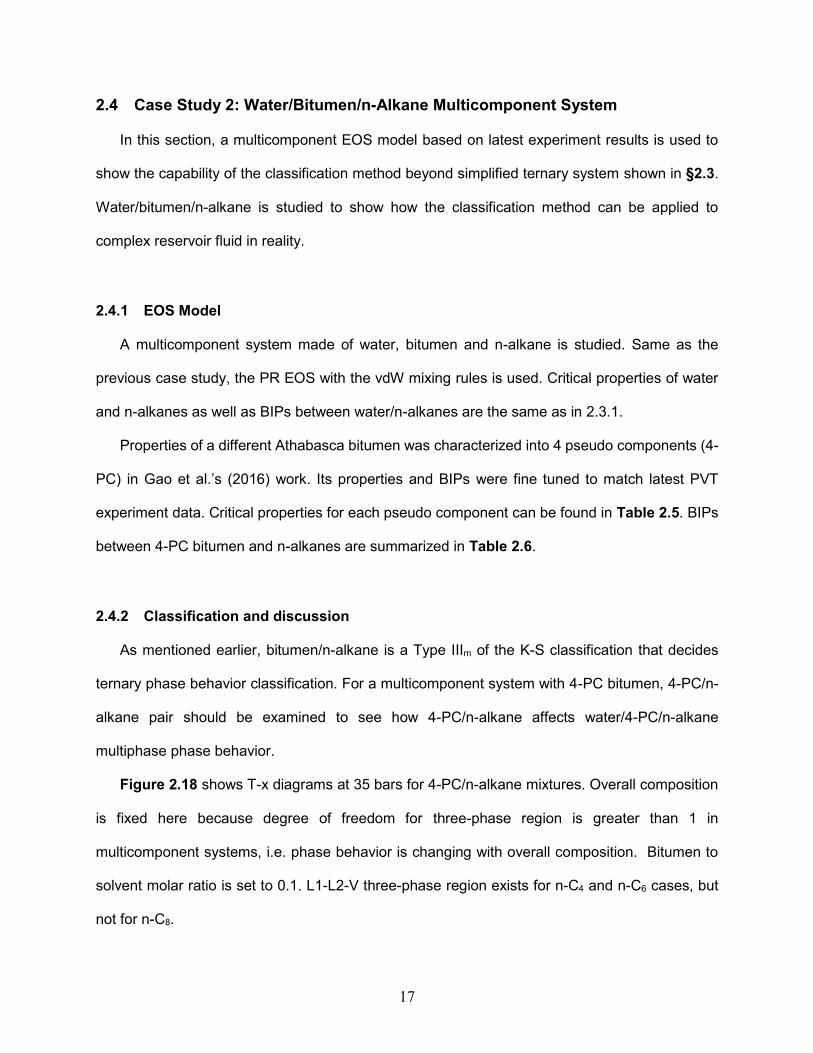
17

2.4 Case Study 2: Water/Bitumen/n-Alkane Multicomponent System

In this section, a multicomponent EOS model based on latest experiment results is used to

show the capability of the classification method beyond simplified ternary system shown in §2.3.

Water/bitumen/n-alkane is studied to show how the classification method can be applied to

complex reservoir fluid in reality.

2.4.1 EOS Model

A multicomponent system made of water, bitumen and n-alkane is studied. Same as the

previous case study, the PR EOS with the vdW mixing rules is used. Critical properties of water

and n-alkanes as well as BIPs between water/n-alkanes are the same as in 2.3.1.

Properties of a different Athabasca bitumen was characterized into 4 pseudo components (4-

PC) in Gao et al.’s (2016) work. Its properties and BIPs were fine tuned to match latest PVT

experiment data. Critical properties for each pseudo component can be found in Table 2.5. BIPs

between 4-PC bitumen and n-alkanes are summarized in Table 2.6.

2.4.2 Classification and discussion

As mentioned earlier, bitumen/n-alkane is a Type IIIm of the K-S classification that decides

ternary phase behavior classification. For a multicomponent system with 4-PC bitumen, 4-PC/n-

alkane pair should be examined to see how 4-PC/n-alkane affects water/4-PC/n-alkane

multiphase phase behavior.

Figure 2.18 shows T-x diagrams at 35 bars for 4-PC/n-alkane mixtures. Overall composition

is fixed here because degree of freedom for three-phase region is greater than 1 in

multicomponent systems, i.e. phase behavior is changing with overall composition. Bitumen to

solvent molar ratio is set to 0.1. L1-L2-V three-phase region exists for n-C4 and n-C6 cases, but

not for n-C8.

18

Accordingly, water/4-PC/n-alkane is examined at 35 bars, with 95 mol% water and 0.1

bitumen-solvent ratio. Figure 2.19 shows T-x diagrams for systems including water. W-L1-L2-V

4-phase region exists for n-C4 and n-C6, but not for n-C8.

In this case, n-C4 and n-C6 are classified as Ternary Type 1 while n-C8 is classified as Ternary

Type 2. It is the L1-L2-V three-phase behavior in bitumen/n-alkane mixture determines the W-L1-

L2-V behavior in water/bitumen/n-alkane multicomponent system. The generic classification

method still holds true for more complicated mixtures like in this case. This is due to the fact that,

ideally, simplified ternary system water/bitumen/solvent is capable of capturing key multiphase

behavior for more complicated reservoir fluids. Classification on simplified ternary systems is a

good representation for reservoir fluids type in reality.

The case study 2 uses a different bitumen as in case study 1. That explains why C6 is Ternary

Type 1 in case study 2 but a Ternary Type 2 in case study 1. Generally, heavier oil turns Ternary

Type 1 into Ternary Type 2.

The significance of the classification for ternary systems is to understand how the miscibility

between solvent and bitumen can affect the bitumen dilution with water and solvent on the

chamber edge. It has been shown through case study 1 and 2 that the separation of two different

oleic phases is possible for Ternary Type 1 system. The existence of the Ternary Type 1 system

of water/bitumen/n-C4 has been observed by Gao et al. (2016) through experiment study. The

EOS model in case study 2 is based on their experiment measurement of water/bitumen/solvent

phase behavior. In their study, L1-L2-V was found coexisted for a bitumen/n-C4 mixture with 97

mol% C4 around 413.25 K and 29.21 bars. In the corresponding ternary system with 62 mol% of

water and 37 mol% of C4, the coexistence of W-L1-L2-V was observed around 433.05 K and

45.76 bars, which is in the vicinity of the complete condensation condition at this pressure. A

separated oleic phase means poor bitumen dilution with solvent. Also, they found that lighter

components in the bitumen was extracted to the L2 phases, and therefore the L1 phase becomes

even more viscous and difficult to flow.

19

2.5 Conclusions

A generic classification method for phase behavior of water/oil/solvent ternary systems was

developed in this chapter. This method classifies ternary systems based on three-phase behavior

in temperature-composition space by investigation of phase behavior of bitumen/solvent, which

falls into Type II, IV or IIIm of the classification by van Konynenberg and Scott (1980).

If the bitumen/solvent binary shows more than one oleic phases within the chamber

edge temperature range, the corresponding water/bitumen/solvent ternary system is

classified as Ternary Type 1; otherwise, it is classified as Ternary Type 2. Here, the

chamber edge temperature range is defied by two extreme cases: the upper

temperature bound is defined as the chamber edge temperature when solvent is not

injected at all, i.e. the SAGD chamber edge temperature; the lower temperature bound

is defined as the chamber edge temperature when bitumen is 100% displaced, i.e. the

complete condensation temperature of water/solvent.

For the specific n-alkane containing bitumen system studied in case study 1, n-alkanes

up to n-C4 are classified as Ternary Type 1, and n-alkanes heavier than n-C4 are

classified as Ternary Type 2. Ternary Type 1 has complex three-phase transitions

among W, L1, L2 and V within the operation temperature range. However, only W, L1

and V exist for Ternary Type 2 phase behavior within coinjection operation

temperature range, from T3p of water/n-alkane to that of water/bitumen.

The classification for case study 1 is subject to several conditions. Higher operation

pressure will turn Ternary Type 1 into Ternary Type 2. Heavier bitumen will turn

Ternary Type 2 into Ternary Type 1. Also, heavier solvents within the same family will

turn Ternary Type 1 into Ternary Type 2.

Case study 2 indicates the possibility of a second oleic phase L2 inside the steam

chamber. The ternary classification method based on bitumen/solvent binary can be

20

applied to multicomponent systems. In the multicomponent system, n-C4 and n-C6 are

Ternary Type 1 because L2 phase exists within the operation temperature range of

steam-solvent coinjection. N-C8 is classified as Ternary Type 2.

21

Figure 2.1 A reproduction of the binary classification method by van Konynenburg and Scott (1980). The vdW EOS was used in their classification method. Λ and ζ are only functions of a and b specific to the vdW EOS. Different regions are divided by enumerating all possible a and b values.

Figure 2.2 Boundaries between Type II, IV and IIIm of the classification by van Konynenberg and Scott (1980). As will be shown in the subsequent figures, they share some common features. Transition from II to IIIm may happen if the binary consists of a hydrocarbon and a non-water component. CO2/n-C10 is Type II, while CO2/n-C13 IV, and CO2/n-C14 IIIm.

22

Figure 2.3 Schematic of typical Type III-HA binary P-T projections. Water/n-C5 is taken as an example. three-phase line is to the left of both of the vapor pressure curves. One critical curve connects UCEP and CP n-C5 and the other one connects CP water and infinity.

Figure 2.4 Schematic of typical Type III binary P-T projections. It is a Type IIIm system to be specific. Bitumen/C3 is taken as an example. three-phase line is between two vapor pressure curves. One critical curve connects UCEP and CP of C3 and the other one connects CP of water and infinity.

23

(1) Type II

(2) Type IV

24

(3) Type IIIm

Figure 2.5 Schematic to show the transition from Type II to IIIm via IV in P-T diagram. Intersection of the S-shaped critical curve with three-phase line or vapor pressure curve results in three different types of phase behavior, and yet very similar.

P↑ P↑ (1) Type III-HA (2) Type IIIm

Figure 2.6 Schematic of van Konynenburg and Scott (1980) Type III-HA and Type IIIm T-x diagrams with increased P (a figure from Deiter and Kraska, 2012). From the bottom to the top, pressure increases. The phase boundary is easy to disappear for IIIm with increasing pressure.

25

(1) Bitumen/n-alkane three-phase curves

(2) Water/solvent three-phase curves

Figure 2.7 Vapor pressure curves and binary three-phase curves of water/bitumen/n-alkane system.

26

Figure 2.8 Water/bitumen T-x diagram at 35 bars. Long dashed line represents three-phase temperature of water/bitumen, which is 515 K. Short dashed lines are tie lines. Solid dots represent critical point or saturated point.

(1) Bitumen/n-C4

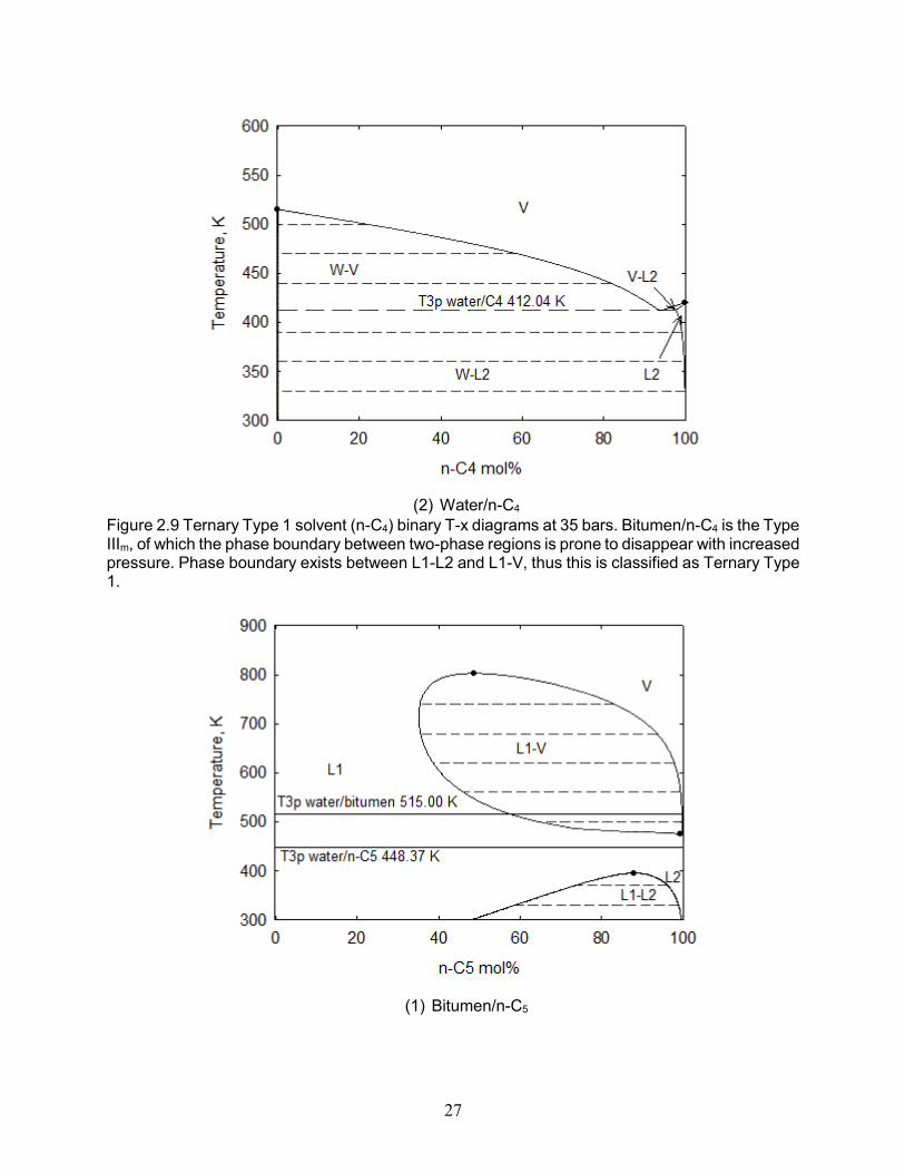
27

(2) Water/n-C4

Figure 2.9 Ternary Type 1 solvent (n-C4) binary T-x diagrams at 35 bars. Bitumen/n-C4 is the Type IIIm, of which the phase boundary between two-phase regions is prone to disappear with increased pressure. Phase boundary exists between L1-L2 and L1-V, thus this is classified as Ternary Type 1.

(1) Bitumen/n-C5

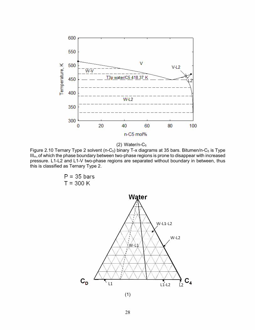
28

(2) Water/n-C5

Figure 2.10 Ternary Type 2 solvent (n-C5) binary T-x diagrams at 35 bars. Bitumen/n-C5 is Type IIIm, of which the phase boundary between two-phase regions is prone to disappear with increased pressure. L1-L2 and L1-V two-phase regions are separated without boundary in between, thus this is classified as Ternary Type 2.

(1)

29

(2)

(3)

30

(4)

(5)

31

(6)

(7)

32

(8)

Figure 2.11 Ternary Type 1 ternary phase behavior at 35 bars. Water/bitumen/C4 case is taken as an example. L1 represents bitumen-rich oleic phase, while L2 solvent-rich oleic phase. As temperature increases, complicated three phase region transition happens. (1) to (2): Only one three-phase region W-L1-L2 exists. (3) W-L2-V starts to emerge on the water/nC4 edge at T3p of water/n-C4. (4) to (6): First, W-L2-V gradually expands. Then, it merges with W-L1-L2 and immediately, W-L1-L2 and W-L2-V reform into W-L1-V and V-L1-L2. (7) to (8): L1 vertex swings towards water/bitumen edge and finally disappears onto water/bitumen edge.

33

(1)

(2)

34

(3)

(4)

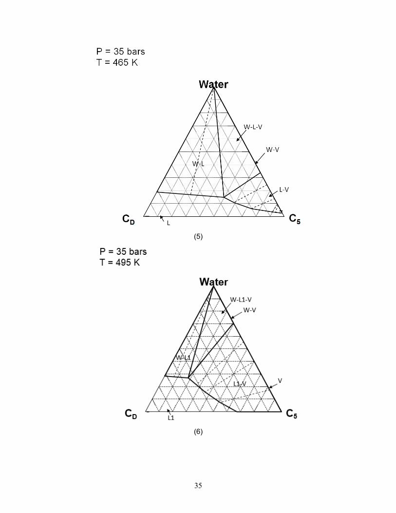
35

(5)

(6)

36

(7)

Figure 2.12 Ternary Type 2 ternary phase behavior at 35 bars. Water/bitumen/C5 case is taken as an example.L1 represents bitumen-rich oleic phase, while L2 solvent-rich oleic phase. (1) to (3): Only one three-phase region W-L1-L2 exists. (4) No three-phase region exists. (5) to (7): W-L1-V emerges from water/n-C5 edge at T3p of water/n-C5. Then, L1 swings from water/n-C5 edge towards water/bitumen edge. W-L1-V disappears at water/bitumen T3p.

37

(1)

38

(2)

Figure 2.13 Typical Ternary Type 1 water/bitumen/n-alkane ternary phase behavior in 3D. Water/bitumen/n-C4 is considered at 35 bars with temperature range from 300 K to 515 K. One continuous spatial solid geometry consists of four different kind of three-phase regions.

39

Figure 2.14 Typical Ternary Type 2 water/bitumen/n-alkane ternary phase behavior in 3D. Water/bitumen/n-C5 is considered at 35 bars with temperature range from 300 K to 515 K. Two separate solid geometries are observed.

40

Figure 2.15 T-x diagram of bitumen/n-C4 binary at 60 bars for case study 1. Increased pressure

eliminates phase boundary between two-phase regions and turn n-C4 into a Ternary Type 2

solvent at 70 bars.

(1) Water/C1

41

(2) Bitumen/C1

Figure 2.16 Binary phase behavior for extreme Ternary Type 1 case: methane. three-phase

temperature of water/C1, bitumen/C1 and saturation temperature of methane are the same.

42

(1)

(2)

43

(3)

(4)

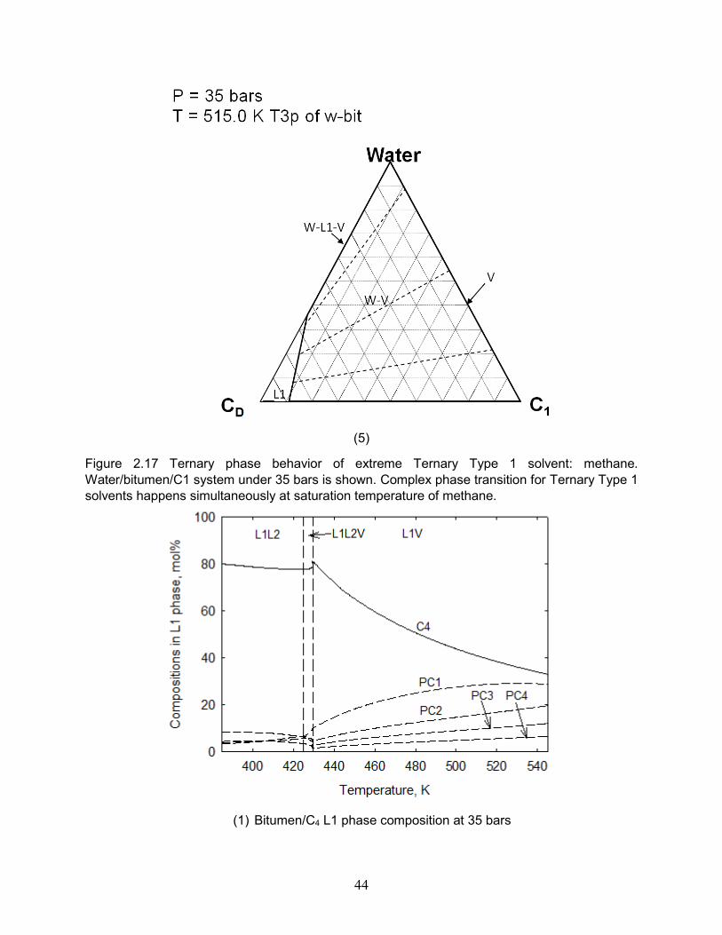
44

(5)

Figure 2.17 Ternary phase behavior of extreme Ternary Type 1 solvent: methane.

Water/bitumen/C1 system under 35 bars is shown. Complex phase transition for Ternary Type 1

solvents happens simultaneously at saturation temperature of methane.

(1) Bitumen/C4 L1 phase composition at 35 bars

45

(2) Bitumen/C6 L1 phase composition at 35 bars

(3) Bitumen/C8 V phase composition at 35 bars

Figure 2.18 Case study 2 isobaric phase behavior of 4-PC bitumen and n-alkane model at 35

bars. Bitumen-solvent ratio is 0.1. The existence of L1L2V of C4 and C6 explains why in Figure

2.17, WLLV exists for C4 and C6. The classification criterion still holds true for multicomponent

systems like this.

46

(1) Water/bitumen/C4 L1 phase compositions at 35 bars


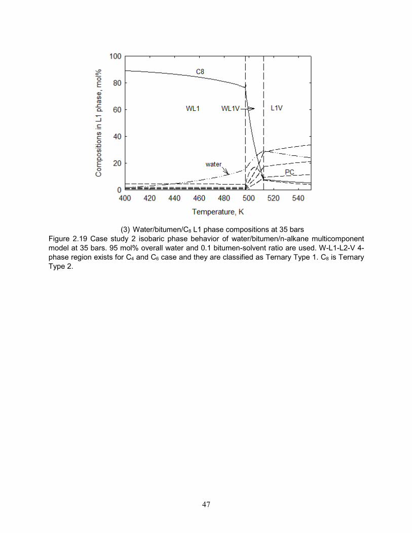
47


Figure 2.19 Case study 2 isobaric phase behavior of water/bitumen/n-alkane multicomponent

model at 35 bars. 95 mol% overall water and 0.1 bitumen-solvent ratio are used. W-L1-L2-V 4-

phase region exists for C4 and C6 case and they are classified as Ternary Type 1. C8 is Ternary

Type 2.

48

Table 2.1 Case study 1 critical properties and molecular weight for water/bitumen/n-alkane ternary

EOS model. Bitumen is characterized as one pseudocomponent, symbolized as CD.

Table 2.2 Case study 1 binary interaction parameters table for water/bitumen/n-alkane ternary

system equilibrium calculation. The upper diagonal of the matrix is neglected because of

symmetry.

BIP C1 C3 n-C4 n-C5 n-C6 n-C7 n-C8 n-C9 n-C10 CD Water

C1 0.000

C3 0.000 0.000

n-C4 0.000 0.000 0.000

n-C5 0.000 0.000 0.000 0.000

n-C6 0.000 0.000 0.000 0.000 0.000

n-C7 0.000 0.000 0.000 0.000 0.000 0.000

n-C8 0.000 0.000 0.000 0.000 0.000 0.000 0.000

n-C9 0.000 0.000 0.000 0.000 0.000 0.000 0.000 0.000

n-C10 0.000 0.000 0.000 0.000 0.000 0.000 0.000 0.000 0.000

CD 0.000 0.067 0.075 0.081 0.088 0.094 0.098 0.102 0.105 0.000

Water 0.732 0.666 0.636 0.607 0.579 0.553 0.527 0.503 0.480 0.169 0.000

Table 2.3 Case study 1 ternary classification sensitivity to pressure. Pressures at UCEP and CP

as well as at which Ternary Type 1 turns into Ternary Type 2 (bifurcation) are summarized.

Pc, bar PUCEP, bar P bifurcate, bar

C3 42.48 43.58 143.95

n-C4 37.96 42.26 43.24

n-C5 33.70 9.20 9.20

n-C6 and plus - <1 <1

Comp TC, K PC, bar ω MW Vc, cc/mol

C1 190.5611 45.9908 0.0157 16.0427 -

C3 369.8278 42.4807 0.1543 44.0961 203

n-C4 425.1222 37.9605 0.2014 58.1228 255

n-C5 469.7000 33.7009 0.2511 72.1495 304

n-C6 507.6000 30.2507 0.3010 86.1762 370

n-C7 540.2000 27.4005 0.3505 100.2029 432

n-C8 568.7000 24.9245 0.3980 114.2296 492

n-C9 594.6000 22.9002 0.4459 128.2563 548

n-C10 617.7000 21.1000 0.4898 142.2830 603

CD 847.1700 10.6381 1.0406 530.0000 1330

Water 647.0960 220.6400 0.3433 18.0100 -

49

Table 2.4 Case study 1 Ternary Type 1 system complex phase transition summary. At 35 bars,

this starts from water/n-alkane three-phase temperature to that of bitumen/n-alkane.

Tsat, K T3p w-sol, K T3p bit-sol, K ΔT3p, K

C1 181.76 181.76 181.76 0.00

C2 289.41 289.54 289.39 0.15

C3 358.89 359.55 357.83 1.72

n-C4 419.99 422.30 412.04 10.26

Table 2.5 Case study 2 bitumen critical properties, molecular weight and composition. Bitumen is

characterized into 4 pseudo components by Kumar and Okuno (2016). Water and n-alkanes

properties are the same as case study 1.

TC, K PC, bar ω MW

Mol% in bitumen

PC1 813.6410 18.9600 0.4393 296.9391 53.46

PC2 1066.1180 13.6800 0.8657 662.8018 23.95

PC3 1244.3200 12.3200 1.0497 1082.6682 14.66

PC4 1452.9860 11.6800 0.8947 2003.4936 7.92

Table 2.6 Case study 2 BIP table for the PR EOS.

n-C4 n-C6 n-C8 PC1 PC2 PC3 PC4 Water

n-C4 0.000

n-C6 0.000 0.000

n-C8 0.000 0.000 0.000

PC1 0.010 0.016 0.015 0.000

PC2 0.015 0.028 0.031 0.050 0.000

PC3 0.028 0.035 0.041 0.050 0.040 0.000

PC4 0.030 0.046 0.055 0.050 0.040 0.030 0.000

Water 0.636 0.579 0.527 0.200 0.200 0.200 0.200 0.000

50

Chapter 3 Analysis of Solvent Distillation

3.1 Introduction

In steam injection or steam/solvent coinjection, mobility of bitumen is enhanced because of

the increased temperature and/or the dilution of bitumen with solvent. Besides, enhanced

displacement efficiency that results in oil saturation that is lower than endpoint oil saturation is

another important mechanism that makes steam-solvent coinjection superior to SAGD.

It was initially observed by Willman et al. (1961) through experiments that an almost zero

residual oil saturation (Sor) was achieved in steam injection. Later, Sor lower than the endpoint oil

saturation was reported in a number of field tests (Blevins et al., 1969; Volek and Pryor, 1972;

Blevins and Billingsley, 1975). The low Sor is due to the distillation of solvent or light to medium

components in the heavy oil. Solvent distillation is defined as the vaporization of distillable

components in residual oil, leaving the heavy components in situ (Willman et al., 1961 and Prats,

1982). The distilled solvents would condense at steam front, dilute the bitumen and increase

displacement efficiency. Condensation, dissolution into bitumen and vaporization of solvent, i.e.

solvent distillation, result in volume shrink of residual oil, even lower than endpoint saturation.

Inside a steam chamber for steam-solvent coinjection, the steam and solvent first condenses

on the edge of the steam chamber. Then the condensed water and solvent will mix with bitumen

and therefore, bitumen is diluted. If temperature is increased, volatile components from the diluted

bitumen may evaporate and therefore the volume of oleic phase shrinks.

Figure 3.1 explains the process of distillation through an imaginary PVT experiment. In a PVT

cell at isobaric conditions, there are initially water phase that contains pure water or both water

and dissolved solvent, and also oleic phase which is a bitumen diluted with solvent and water. If

the pressure in the PVT cell keeps a constant and temperature is gradually increased, the light

component from the liquid phases, i.e. water and solvent, will evaporate to the vapor phase. As a

51

result, the volume of the oleic and aqueous phases shrinks. The oleic phase becomes more

viscous as water and solvent evaporated.

However, the solvent distillation is not yet analytically quantified so far. Willman et al. (1961)

develops a mathematical description for steam drive performance. They measured Sor and

incorporated the measurements into their calculation. Johnson et al. (1971) modeled volumetric

change of oleic phase due to distillation as a function of solvent accumulation on chamber edge.

However, the models mentioned above did not directly discuss residual oil saturation as a result

of phase behavior.

Keshavarz et al. (2014) showed the mechanism of enhanced displacement efficiency by

solvent distillation through ternary diagrams. In order to reduce the oil saturation to less than

endpoint So, solvent should first accumulate on chamber edge, then phase splits and solvent

evaporates as temperature increases. Following this explanation, Keshavarz and Chen (2014)

modeled the average Sor inside the steam chamber mathematically, using Raoult’s law and

correlated temperature change during distillation. Raoult’s law is only suitable for ideal solutions.

Besides, they assumed only maximum one oleic phase and immiscibility between hydrocarbon

and water. Therefore, accurately modeled phase behavior and reduced Sor as a result of phase

behavior change were not an emphasis in their research.

In this chapter, the first thermodynamic tool is proposed to estimate displacement efficiency

enhanced by solvent distillation. The algorithm solves analytical Sor with a few inputs compared

to numerical simulation. The tool is based on the systematic phase behavior study including

multiphase and multicomponent in Chapter 2. This model helps explain reduced Sor in steam or

steam/solvent injection. Differences between two types of n-alkanes proposed in Chapter 2 are

discussed. Comparisons of Ternary Type 1 and 2 solvents are done through sensitivity analysis

and numerical simulations.

52

3.2 Mechanistic Calculation of Distillation using an EOS

The solvent distillation in SAGD and steam-solvent coinjection begins with solvent and water

mixing with bitumen on the edge of steam chamber. As described by Keshavarz et al. (2014),

chamber edge is defined where the phase transition occurs between WL and WLV as shown in

Figure 3.2. On the chamber edge, the overall composition is located on the WL edge of WLV tie

triangle and vapor phase saturation is zero. The W phase contains 100% water, and the L phase

contains water, bitumen and solvent. If temperature is increased from the one shown in

Figure 3.2 (1), distillable components will evaporate from the W and L phases. Distillable

components may include water from the W and L phases and solvent from the L phase. These

distillable components make up the V phase inside the chamber, in which W-L-V coexist. Figure

3.2 (2) shows the chamber edge condition in a reservoir. The overall composition is resided on

the boundary between W-L and W-L-V.

Based on the systematic phase behavior study in Chapter 2, another situation of chamber

edge condition specific to Ternary Type 1 n-alkanes is also possible, which is shown in

Figure 3.3. If the chamber edge temperature is low, W-L1-L2 coexists on the chamber edge. L1

is the bitumen-rich oleic phase and L2 the solvent-rich oleic phase. In this chamber edge condition,

overall composition can be located on or inside W-L1-L2 tie triangle. If temperature is increased

from Figure 3.3 (1), W, L1 and L2 will evaporate simultaneously. Figure 3.3 (2) shows a

schematic of chamber edge for this situation. W-L-L is outside the chamber and W-L-V inside the

chamber. The overall composition resides within the W-L1-L2 in the ternary diagram.

One special case in Ternary Type 1 solvent is methane (C1). The live bitumen contains mainly

C1 as the solution gas. Bitumen has limited capacity to maintain solution gas such as C1. Usually,

live bitumen has a gas-oil ratio (GOR) somewhere between 0 to 5 m3/m3. If the Athabasca bitumen

in case study 1 of Chapter 2 is considered, a GOR of 5 m3/m3 is corresponding to 10 mol% of C1

in the Athabasca bitumen. If only steam is injected in to the bitumen reservoir, C1 will evaporate

from the live bitumen. Therefore, the chamber edge temperature will be affected by the

53

evaporated C1. Figure 3.4 shows the ternary phase behavior on chamber edge at 35 bars when

the Athabasca bitumen described in case study 1 of Chapter 2 is considered. The GOR of the live

bitumen is 5 m3/m3 (or 10 mol% C1 in bitumen). If a zero GOR is considered, the chamber edge

temperature will be the same as three-phase temperature of water/bitumen at 35 bars, i.e. 515.00

K. The chamber edge temperature is lowered from 515.00 K to 442.76 K if a 10 mol% C1 is

dissolved in bitumen. Under this condition, only one oleic phase, L1, exists on the chamber edge.

In the mechanistic study in this section, the bitumen is assumed to be a dead bitumen, i.e. no

solution gas is considered in the bitumen. Later on in this thesis, the effect of non-zero GOR on

the chamber edge condition and displacement efficiency will be revisited.

Distillation of water is assumed to be constrained by endpoint water saturation (Swr) inside the

steam chamber. Endpoint water saturation is the irreducible water saturation. The irreducible

water cannot be taken away by flow, usually because the water is stuck in the pores or is attached

to the surface of rock. The irreducible water saturation is affected by the porosity, pore structures,

rock compositions and wettability on the rock surface. The tighter the pore, or the more

heterogeneous the porosity, the greater the irreducible water saturation is. Also, the more

hydrophilic the rock surface, the greater the irreducible water saturation. It is assumed that the

distillation ends when water saturation reaches irreducible level, because wet steam is injected in

SAGD or coinjection, and heat losses always exist. This means water in the state of liquid always

exists. The water condensate occupies the pore space and is a source of the water saturation

inside a chamber. The part of water that is in the excess of the residual water saturation flows,

and leaving the residual amount inside the chamber. In the end of distillation, the evaporation and

condensation of water will reach a dynamic balance. This chapter is to quantify how much solvent

is distilled from L phase if water saturation is reduced to a given Swr.

Resulting Sor depends on many factors, such as operation pressure, bitumen properties,

volatility of solvent, accumulation of solvents and water on the chamber edge, and endpoint phase

54

saturations decided by rock properties. Due to the complexity, simplifying assumptions are made

and sensitivities of each affecting factors are analyzed.

Assumptions for simplification are listed below.

Isobaric condition during the distillation process. During steam injection, the pressure

inside and outside the steam chamber is assumed to be the same as injector

bottomhole pressure. Since the oil saturation and water saturation are no more than

the endpoint saturations, liquid phases cannot flow. The flowing vapor phase has very

high mobility so that it does not require high pressure difference to flow inside a steam

chamber. This justifies the isobaric assumption. In reality, the pressure is the highest

near the injector, and gradually decreases as it becomes distant from the injector.

However, the difference in pressure of near wellbore area and area far from wellbore

is negligible. This is because the propagation of pressure wave is faster than the

propagation of steam chamber.

Chamber edge is defined where phase transition happens between WL (or WLL) and

WLV. Take water/bitumen/n-alkane ternary system as an example, two types of

chamber edge conditions are possible. For Ternary Type 1 solvents (as C3 in

), W-L1-L2 or simply W-L1 appears on chamber edge. For Ternary Type 2 solvents,

only W-L1 on chamber edge is possible.

Fixed overall composition is assumed during distillation of water and solvent. In reality,

overall composition on the chamber edge cannot be controlled directly. This is done

by manipulation of the injection strategy, i.e. the injection pressure, the injection rate,

and/or the injection ratio of steam and solvent. Also, from the chamber edge to inside

the chamber edge, flow always exists. This unavoidably results in a change in overall

composition during the distillation. However, without a fixed overall composition, it is

impossible to define the beginning and the end of the distillation, as will be shown soon

in this section. This assumption will give the most conservative estimation for analytical

55

Sor. This quantification method only provides a simplified way to explain distillation,

without consideration of mass balance or energy transfer as in numerical simulation.

Water saturation cannot be lower than irreducible water saturation Swr. As

aforementioned reason in this section, water always exists in the reservoir.

Saturations can be calculated in the following way,

𝑆𝑗 =𝛽𝑗𝜌𝑗

∑ 𝛽𝑘𝜌𝑘𝑁𝑝𝑘=1

(3.1)

where j is the phase, which can be W, L or V phase, 𝑆𝑗 is the saturation of phase j, 𝛽𝑗 the mole

fraction of phase j, 𝜌𝑗 is the density of phase j, and Np is the number of phases. 𝛽𝑗 can be either

analytically determined by the Rachford-Rice algorithm, or geometrically determined by the

material balance or the so-called lever rule. An example using the lever rule is given in Figure

3.5. The phase mole fractions of W, L and V phases can be determined by the geometric relations

below,

𝛽𝑤 = 𝑙𝑏

𝑙𝑎 + 𝑙𝑏, 𝛽𝑜 =

𝑙𝑑

𝑙𝑐 + 𝑙𝑑, 𝛽𝑔 =

𝑙𝑓

𝑙𝑒 + 𝑙𝑓

(3.2)

where w, o and g represents the W, L and V phase respectively, and 𝑙 represents the length of

each section indicated in Figure 3.5.

The algorithm for analytical Sor for solvent distillation is presented as follows:

Step 1 Make a phase behavior model at pressure P with an EOS and proper mixing rules.

If a cubic EOS with the vdW mixing rules is considered, basic EOS inputs include the

operation pressure, critical properties and binary interaction parameters, and volume

shift parameters.

Step 2 Define chamber edge conditions. Set T=Tedge.

56

Chamber edge temperature (Tedge) can be uniquely determined with the overall

composition based on assumption 2. For an example, if at most three phases coexist,

Tedge can be determined via simple geometric relationship using the lever rule. (1) If

W-L exists on chamber edge, 𝛽𝑔 = 0, i.e. 𝑙𝑓 = 0. (2) If W-L1-L2 exist on chamber edge,

Tedge would be the unique temperature where W-L1-L2 turns into W-L1-V for Ternary

Type 1 (Figure 2.13). In general, a Rachford-Rice algorithm capable of negative flash

can be used to determine the temperature at which vapor phase mole fraction is zero.

Step 3 Calculate phase mole composition 𝛽𝑗.

𝛽𝑗 can be calculated using the robust multiphase Rachford-Rice algorithm of Okuno

et al. (2010) with K-values based on the EOS at z, P, and T.

Step 4 Calculate phase molar density and phase saturation.

One of the convenient methods to calculate saturations is described in Appendix B.

Step 5 Check if Sw > Swr.

- If so, increase T by 0.01 K and go back to Step 3.

- If not, continue to the next step.

Step 6 Output residual saturations at upper T bound (TSwr) at which Sw is Swr.

The distillation is considered come to an end when Sw reaches Swr in the analytical

solution. The corresponding temperature TSwr can be found by both Equation 3.1 and

3.2, when Sw=Swr.

A flowchart for this algorithm is shown in Figure 3.6. To sum up, inputs of the analytical Sor

requires EOS and mixing rules, critical properties, BIPs, overall composition and endpoint

saturations. Outputs include saturation change with temperature during distillation.

57

3.3 Case Study 1: Water/Bitumen/n-Alkane Ternary System

The algorithm presented in §3.2 are applied to water/bitumen/n-alkane ternary system

described in §2.3.1. Bitumen is characterized as one pseudo component in the EOS model. An

example calculation for n-C5 is first given to show how the algorithm work to solve analytical Sor.

Then, sensitivity analysis is done regarding solvent volatility of n-alkanes, chamber edge solvent

accumulation, chamber edge water concentration (zw), irreducible water saturation (Swr) and

endpoint oil saturations of reservoir rock.

3.3.1 Example Calculation

Analytical Sor for n-C5 distillation is shown as an example. The operation pressure is set to 35

bars, which makes n-C5 a Ternary Type 2 solvent. The overall composition at the chamber edge

is assumed to be 98 mol% water and 1.2 mol% n-C5. Swr is set to 0.25. Conditions for this example

are summarized in Table 3.1.

Figure 3.7 (1) visualizes the whole process of distillation through ternary prism. It is assumed

that the overall composition is constant throughout the distillation. Chamber edge can be found

when overall composition is located on the W-L1 edge of W-L1-V tie triangle. This is when n-C5

and water starts to evaporate from liquid phases, and when vapor phase starts to emerge. As

temperature increases, the L1 vertex of the tie triangle swings towards the water/bitumen edge in

composition space due to solvent evaporation from L1 phase until Swr is reached. Analytical Sor

can be calculated at TSwr.

Figure 3.7 (2) shows mass transfer from liquid phases to vapor phase during distillation

process. On the chamber edge, overall composition is located on the W-L1 edge of W-L1-V and

Sg is zero. As temperature increases, due to the evaporation of solvent and water from L1 phase,

L1 contains a higher molar fraction of bitumen and a smaller fraction of solvent. This makes L1

vertex of W-L1-V getting closer to the water-bitumen edge and therefore So is reduced. Besides,

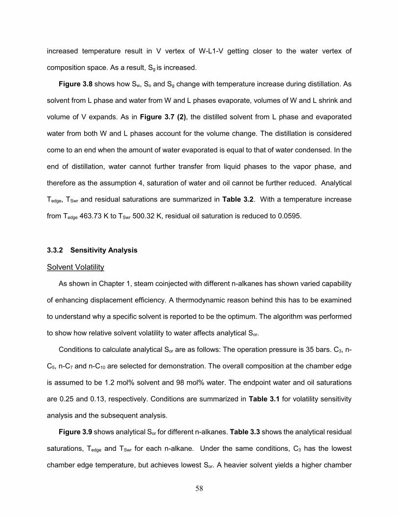
58

increased temperature result in V vertex of W-L1-V getting closer to the water vertex of

composition space. As a result, Sg is increased.

Figure 3.8 shows how Sw, So and Sg change with temperature increase during distillation. As

solvent from L phase and water from W and L phases evaporate, volumes of W and L shrink and

volume of V expands. As in Figure 3.7 (2), the distilled solvent from L phase and evaporated

water from both W and L phases account for the volume change. The distillation is considered

come to an end when the amount of water evaporated is equal to that of water condensed. In the

end of distillation, water cannot further transfer from liquid phases to the vapor phase, and

therefore as the assumption 4, saturation of water and oil cannot be further reduced. Analytical

Tedge, TSwr and residual saturations are summarized in Table 3.2. With a temperature increase

from Tedge 463.73 K to TSwr 500.32 K, residual oil saturation is reduced to 0.0595.

3.3.2 Sensitivity Analysis

Solvent Volatility

As shown in Chapter 1, steam coinjected with different n-alkanes has shown varied capability

of enhancing displacement efficiency. A thermodynamic reason behind this has to be examined

to understand why a specific solvent is reported to be the optimum. The algorithm was performed

to show how relative solvent volatility to water affects analytical Sor.

Conditions to calculate analytical Sor are as follows: The operation pressure is 35 bars. C3, n-

C5, n-C7 and n-C10 are selected for demonstration. The overall composition at the chamber edge

is assumed to be 1.2 mol% solvent and 98 mol% water. The endpoint water and oil saturations

are 0.25 and 0.13, respectively. Conditions are summarized in Table 3.1 for volatility sensitivity

analysis and the subsequent analysis.

Figure 3.9 shows analytical Sor for different n-alkanes. Table 3.3 shows the analytical residual

saturations, Tedge and TSwr for each n-alkane. Under the same conditions, C3 has the lowest

chamber edge temperature, but achieves lowest Sor. A heavier solvent yields a higher chamber

59

edge temperature, but also higher Sor. However, from C3 to C7, the differences in terms of

analytically calculated Sor is less than 1% under the conditions examined.

Ternary diagrams at Tedge and TSwr are shown in Figure 3.10. With a fixed overall composition,

bitumen-solvent ratio on the chamber edge is set to be the same for each solvent. What makes

each solvent different is the water content in oleic phase. The heavier the solvent, more water is

dissolved in L phase on the chamber edge because Tedge is higher. At the end of distillation where

Swr is about 0.25, L phase of lighter solvents contains a smaller proportion of solvent.

The incremental temperature (ΔT) during distillation, i.e. the difference between TSwr and Tedge,

is summarized in Figure 3.11. Also, the amount of solvent and water distilled from liquid phases

throughout the distillation process is shown in Figure 3.12. The ratio of evaporated water to

solvent for each volatility case is shown in Figure 3.13. Lighter solvents can achieve greater

temperature increase during distillation as a result of lower chamber edge temperature. Besides,

lighter solvent allows relatively less water evaporation and more solvent distillation from liquid

phases. Relative volatility of water to solvent is smaller for lighter solvents. Analytical solution

shows water component transfers only from the W phase to the V phase, and n-alkane only

transfers from the L phase. The total water content in the L phase remains almost a constant.

More C3 distilled from the L phase into the V phase, and less water transferred from the W phase

to the V phase. Therefore, more oil saturation reduction is achieved by C3. Both higher

temperature increase and lower relative volatility between water and solvent for lighter solvents

explains why lighter solvents achieves lower Sor during distillation.

If a live bitumen is used with C1 as the solution gas, the displacement efficiency can be further

improved for steam-solvent coinjection, because C1 is more volatile than any other n-alkanes.

However, the appearance of C1 in the bitumen may detriment chamber edge temperature for

steam-solvent coinjection as C1 evaporates into the V phase.

60

Pressure

Operation pressures can significantly affect phase behavior. As described in Chapter 2, n-C4

can be converted from Ternary Type 1 to Ternary Type 2 if operation pressure is increased from

35 to 60 bars. It is important to discuss analytical Sor sensitivity to pressure due to distillation.

Overall composition is set to 98 mol% water and 1.2 mol% solvent. Endpoint saturations are

0.25 and 0.13 for aqueous and oleic phase respectively. 3 different pressures are used to perform

analytical Sor, 15, 35 and 60 bars (Table 3.1).

Figure 3.14 shows analytical Sor sensitivity to pressure for n-alkane solvents. Table 3.4

summarizes analytical residual saturations. Increased operation pressure improves displacement

efficiency for all the volatility cases. At high pressures such as 35 and 60 bars, differences in

terms of displacement efficiency of Ternary Type 1 and light Ternary Type 2 solvents are less

than 0.5%. Generally, lighter solvents are less affected by pressure increase than heavier ones.

By further increase pressures from 35 bars, limited Sor reduction can be achieved for Ternary

Type 1 and light Ternary Type 2 solvents.

Figure 3.15 shows the ΔT during distillation for each volatility cases at three different

pressures. Mole fraction of water and solvent evaporated from liquid phases during distillation is

summarized in Figure 3.16. The relative amount of evaporated water to solvent is shown in

Figure 3.17. Generally, increased pressure results in increased ΔT; however, there are a few

exceptions mainly because of differences between T3p of water/bitumen and water/solvent is not

monotonically changing with pressure. The increased ΔT allows more solvent to evaporate. With

increased pressure, C3 (Ternary Type 1) is limited to let more solvent to evaporate from L phase

because the solvent in residual oil is already too low at low pressures. Analytical Sor of C10

(Ternary Type 2) is more sensitive to pressure increase than lighter solvents. This is because of

the existence of enough distillable solvent in residual oil and therefore increased ΔT allows more

solvent to evaporate.

61

Solvent Accumulation

Solvent dissolution in L phase in the vicinity of chamber edge is an important mechanism that

results in enhanced displacement efficiency and drainage rate. Effective solvent dissolution

through convection improves bitumen recovery and oleic phase mobility. Recall the differences

between two types of n-alkanes ternary phase behavior. A solvent-rich oleic phase may exist

other than the bitumen-rich oleic phase for Ternary Type 1. Two types of solvents may have very

different chamber edge conditions.

Two types of chamber edge condition exist for Ternary Type 1: when solvent concentration is

low, overall composition sits on the W-L1 edge of W-L1-V; when solvent concentration is high,

overall composition is inside the W-L1-L2 region. The latter situation has separated oleic phases

on the chamber edge, which indicates poor solvent dissolution into bitumen.

Here, a series of solvent concentration is plotted against analytical Sor for selected n-alkanes.

Operation pressure is set to 35 bars. Water concentration, Swr and endpoint So are 98 mol%,

0.25 and 0.13 respectively (Table 3.1).

Table 3.5 summarizes the analytical Sor and Figure 3.18 shows Sor sensitivity to solvent

concentration for selected n-alkanes. In general, Sor for all solvents are sensitive to solvent

concentration change. Lighter solvents are more sensitive to solvent concentrations than heavier

ones although C3 to n-C7 shows very similar sensitivity to solvent concentration change. Sor is

almost halved if solvent dissolution in bitumen is doubled for C3 to n-C7. Also, there should be a

threshold solvent accumulation to cause oil saturation lower than 0.13, the endpoint oil saturation.

Heavier solvents need more solvent accumulation to result in similar Sor as lighter solvents do. If

the curves of the analytical solutions are extrapolated from the left-hand side, they will intersect

with the endpoint So line. The corresponding solvent concentration of the intersects represent the

minimum solvent concentration to result in reduced Sor lower than So. When the solvent

concentration is 2 mol% on the chamber edge, the analytical Sor should be theoretically zero.

62

Figure 3.19 shows ΔT during distillation under three selected solvent concentrations. Figure

3.20 shows the amount of water and solvent evaporated from liquid phases during distillation.

Figure 3.21 shows the relative amount of water distilled to that of solvent. One of the reasons is

the increased ΔT due to lowered chamber edge temperature as a result of increased solvent

concentration, which allows more solvent to evaporate. Besides, volatile solvent has more

incremental solvent evaporation due to increased solvent dissolution in bitumen. For heavier

solvent like C10, increased solvent concentration may even result in more water evaporation than

that of lower solvent concentration case. This is correspondent with the sensitivity of analytical

Sor to solvent concentration in Figure 3.18. In the competition of solvent and water evaporation,

lighter solvent is superior to heavier solvents in distillation capability.

Water Concentration in overall composition

As the lever rule indicates, relative position of overall composition inside a tie triangle together

decide the saturation of each phase. Besides bitumen-solvent ratio, sensitivity analysis for water

concentration should also be conducted. Conditions are 35 bars, 1:4 bitumen-solvent ratio, 0.25

Swr and 0.13 Sor, which are summarized in Table 3.1.

Figure 3.22 and Table 3.6 show analytical Sor for a series of water concentration. With 1 mol%

of water concentration increase, an estimated 1.5% of oil saturation can be reduced for C3 and

3% for C10. Therefore, if water concentration is increased, the Sor of heavier solvents is more

affected than lighter ones. Also, for 1:4 bitumen-solvent ratio, each solvent has a threshold water

concentration to result in reduced Sor.

Figure 3.23 shows ΔT during distillation for selected water concentration cases. Also, water

and solvent evaporated from liquid phases during distillation are summarized in Figure 3.24.

Relative volatility of water to solvent is shown in Figure 3.25. Increased global water accumulation

increases ΔT for all the cases. This allows more water and less solvent to transfer from liquid

63

phases to vapor phase. Another observation is that the trend of mole fraction of distilled solvent

is not monotonically changing with CN for C3 case, because the overall composition resides in W-

L1-L2 tie-triangle on the chamber edge of C3 case. The degree of freedom does not allow for the

coexistence of four phases (W-L1-L2-V) inside a chamber. As a result, the evaporation of L2

phase cannot be counted into the solvent evaporation. Despite that, the increased water

concentration correspondingly reduces solvent overall concentration and oil saturation on the

chamber edge. Improved Sor by increased water concentration is a combined result of increased

ΔT and less solvent content to evaporate.

Endpoint Saturation

As mentioned earlier, competition between water and solvent evaporation explains lower Sor

achieved by lighter solvents as a result of greater temperature increase. Swr as an important

constraint in the algorithms of analytical Sor should be examined. However, in reality, Swr may not

affect phase behavior in reservoir as much direct as in the analytical solution, because change in

Swr results in very different relative permeability curves, and therefore alters the flow inside the

reservoir. Therefore, the consequence of changed Swr may be hard to quantify in simulation study.

Conditions are 35 bars, 98 mol% water concentration, 1.2 mol% solvent, 0.13 Sor. Three

different Swrs, 0.10, 0.25 and 0.40, are examined (Table 3.1).

Figure 3.26 and Table 3.7 show the analytical solutions of Sor under different Swr. Lowered

Swr significantly reduces Sor for all n-alkanes. Heavier solvents are more affected by Swr reduction.

At 0.10 Swr, all the n-alkanes results in very similar Sor.

Figure 3.27 shows increased ΔT because of lowered Swr for all the cases. In Figure 3.28, the

amount of solvent and water evaporated from liquid phases are summarized. More solvent is

allowed to evaporate with increased ΔT as a result of lowered Swr. Figure 3.29 shows the relative

volatility of all the n-alkane cases compared to water under different Swr conditions. From those

figures, the Sor is closely related to whether temperature can be further increased and whether

64

more solvent can be distilled from L phase, as a result of solvent competition with water. C10 case

has the greatest incremental water and solvent evaporation compared to lighter solvents, it is the

most sensitive solvent to Swr.

As mentioned earlier, threshold water or solvent concentration exists so that oil saturation can

be reduced to lower than endpoint So. Lower endpoint So requires more solvent accumulation to

result in reduced Sor.

3.4 Case Study 2: Water/Bitumen/n-Alkane Multicomponent System

The algorithm is not limited to ternary systems with up to three phases such as case study 1

in §3.3. In this section, the algorithm is applied to a multicomponent EOS model described in

§2.4.1 with up to four phases. The system contains water, bitumen characterized as four pseudo

components and n-alkane solvent. Descriptions of holistic EOS model can be found in §2.4.1.

What makes case studies 1 and 2 different from each other is the additional degrees of

freedom because more components are used in case study 2. The Ternary Type 1 n-alkanes in

a ternary system cannot have L2 and V phase at the same time inside steam chamber, i.e., L2

on the chamber edge, if exists, will disappear the instant solvent starts to evaporate. However, in

a multicomponent system like in case study 2, W-L1-L2-V coexist inside the chamber before L2

totally disappears. This characteristic of multicomponent systems makes it possible to probe into

the differences between two types of n-alkanes in distillation process.

The conditions for the algorithm performances are, 35 bars pressure, 1:10 bitumen-solvent

ratio, 95 mol% global water concentration, 0.25 Swr and 0.13 endpoint So. The analytical So is

plotted against total molar enthalpy (Ht), which can be calculated by equations below,

𝐻𝑡 = ∑ 𝛽𝑗𝐻𝑗

𝑁𝑝

𝑗=1

(3.3)

65

𝐻𝑗 = ∑ 𝑥𝑖𝑗𝐻𝑖𝐼𝐺

𝑁𝑐

𝑖=1+ 𝐻𝑒𝑥𝑐𝑒𝑠𝑠

(3.4)

where 𝐻𝑡 is the total molar enthalpy, Np total phase number, Nc total component number, 𝛽𝑗

phase j mole fraction, 𝐻𝑗 molar enthalpy of phase j, 𝐻𝑖𝐼𝐺 molar enthalpy of ideal gas for component

i, 𝑥𝑖𝑗 mole fraction of component i in phase j, and 𝐻𝑒𝑥𝑐𝑒𝑠𝑠 excess molar enthalpy between real and

ideal fluid mixtures.

Table 3.8 shows analytical residual saturations for n-C4, n-C6 and n-C8 cases. More volatile

solvents need greater temperature increase to achieve lower Sor. Figure 3.30 shows Ht changes

with temperature. The temperature range where distillation happens is labeled out. The mixture

containing n-C8 requires more energy than lighter solvents to increase temperature by 1 K.

However, n-C8 needs less ΔT to achieve Sor than lighter ones. Therefore, as a whole, lower Sor

achieved by volatile solvents is a result of larger energy requirements due to larger temperature

increase.

Figure 3.31 shows analytical So changing with Ht. Lighter solvents need more energy injected

to achieve better Sor. As in §2.4 , n-C4 and n-C6 are classified as Ternary Type 1 and n-C8 Ternary

Type 2. On chamber edge, W-L1-L2 may coexist for Ternary Type 1 solvents while only W-L1 is

possible for Ternary Type 2 solvents. When Ternary Type 1 solvent starts to evaporate on the

chamber edge, L1 and L2 evaporates together with W, however, L2 evaporates much faster than

L1, since L2 is a separated phase with much more volatile contents than L1. This results in rapid

reduction in oil phase saturation in the beginning of distillation for Ternary Type 1 when L2 is not

totally gone. Table 3.9 shows average △ Ht per unit So reduction calculated for both W-L1-L2-V

and W-L1-V regions of Ternary Type 1. The existence of the solvent-rich oleic phase L2 is

beneficial in terms of So reduction because much less energy is required for W-L1-L2-V region to

reduce So than W-L1-V region. Since n-C6 has a larger temperature range for W-L1-L2-V

66

compared to n-C4, n-C6 is on average more energy efficient to reduce oil saturation, even slightly

greater than n-C8.

3.5 Simulation Case Study

The CMG STARS (Computer Modelling Group, 2013) is used for simulation study of steam/n-

alkane coinjection. Half of a reservoir with dimensions of 70×37.5×20 (m) is divided into 70×1×20

gridblocks. A pair of horizontal well with length of 37.5 m is placed at the left end of the reservoir.

See Table 3.10 for summary of reservoir properties and other simulation parameters. The relative

permeability for each phase is shown in Figure 3.32.

1 mol% of methane is considered as the solution gas in initial bitumen. This is corresponding

to a GOR of 0.44 m3/m3. Altogether, four components exist throughout the simulation: water,

bitumen as one pseudo component, single-component n-alkane and methane. K-values are

tabulated based on the EOS model described in Chapter 2 using WINPROP (2013). WINPROP

performs phase equilibrium calculations to obtain K-values using the PR EOS and the vdW mixing

rules if solvent is insoluble in the aqueous phase. When solvent is soluble in aqueous phase, the

Henry’s law is initiated for aqueous phase fugacity calculation (Nghiem and Li, 1984). However,

the way of WINPROP using Henry’s law heavily relies on correlations regressed upon commonly

seen soluble molecules such as n-alkanes, CO2 and SO2. It may have limited accuracy for

solvents that behaves very different from n-alkanes, CO2 and SO2. Besides, K-values are

tabulated in the WINPROP with a constant overall composition. That is, K values from the

WINPROP are only dependent on temperature and pressure. Here, a rough estimation of

chamber edge overall composition, 90 mol% water and 10 mol% hydrocarbon, is used to tabulate

K-value tables. Since STARS allows only one oleic phase and up to three phases, K-values

tabulated ignore the existence of solvent-rich oleic phase (L2).

67

Reliable viscosity and density models from Venkatramani and Okuno (2016) are used. In

STARS, non-linear mixing of liquid phase viscosity is used. A detailed description of how the non-

linear viscosity models were obtained can be found in there paper. A linear mixing of pure

component densities is used for liquid phases density. Densities are summarized in Table 3.11

and Table 3.12. The vapor phase is modeled as ideal gas and its density follows ideal gas EOS

prediction in STARS.

The injection well operates at a constant 35 bars and the production well at a constant 15

bars. The whole simulation project lasts for 10 years. A 6-month reservoir preheating is

considered at the beginning of simulation. Two injection strategies are considered here: first,

solvent is coinjected with steam at a constant concentration of 2 mol% throughout the simulation;

second, same strategy is used as the first one initially, and then stop injecting solvent immediately

the steam chamber reaches the outer reservoir boundary. The second strategy is used because

the bitumen drainage rate slows down in the late stage of bitumen recovery. It would be

economically beneficial to stop injecting solvent and recovery the retained solvent. Here, C3, n-

C5, n-C7 and n-C10 are selected as pure solvents to be coinjected with steam. C3 is a Ternary

Type 1 solvent at 35 bars, while the rest are Ternary Type 2. Recovery factor, cumulative steam-

oil ratio (CSOR) and solvent recovery are shown in Figure 3.33 to Figure 3.38 for two different

strategies.

In general, Type 2 solvents (C5, C7 and C10) are more efficient than Type 1 (C3) in terms of

bitumen recovery, SOR and solvent recovery. In Figure 3.33 and Figure 3.36, Type 2 solvents

are able to recovery more bitumen faster. Type 2 higher chamber edge temperature and efficient

mixing of solvent with bitumen account for Type 2 efficiency of bitumen recovery.

In Figure 3.34, CSOR is plotted against bitumen recovery factor for the first strategy. For

same amount of bitumen recovered, lower SOR is desired because it indicates less steam amount

required. All n-alkane solvents show improvement in CSOR compared to steam-only injection

case; however, Ternary Type 2 solvents demand less steam injection to produce same amount

68

of bitumen as Ternary Type 1 solvents. Each Ternary Type 2 solvent shows very similar SOR to

produce same amount of bitumen. In contrast, Figure 3.36 shows CSOR against bitumen

recovery factor for second strategy. Steam-only injection at later simulation stage results in

increase of CSOR compared to that of Figure 3.34. However, Ternary Type 2 solvents are still

better than Ternary Type 1 in terms of CSOR.

In Figure 3.35, solvent recovery is plotted against bitumen recovery factor. Ternary Type 1

solvent needs more barrels of solvent retention to achieve the same amount of bitumen recovery

as Ternary Type 2. Figure 3.38 shows solvent retention after switching to the second operation

strategy. By switching to the second strategy, steam-only injection at later simulation stage, Type

2 solvents can be more efficiently recycled. Because Ternary Type 2 solvents are more narrow-

boiled in the whole W-L1-V region than Ternary Type 1 solvents, as is shown in §3.4 case study

2. With little temperature increase, L1 phase composition is able to change more rapidly for

Ternary Type 2 than Type 1. Besides, steam-only injection increases water concentration in the

whole reservoir. L1 phase saturation of Ternary Type 2 is more sensitive to global water

concentration as is shown in §3.3, case study 1. Therefore, Ternary Type 2 solvents can be more

efficiently recycled than Type 1.

It is not possible to quantitatively validate the result of analytical Sor through simulation study

for the following reason. For one thing, the simulated reservoir is not a closed system. Overall

composition is changing from the chamber edge to inside the chamber. For another thing, in order

to compare the Sor between the two methods, same P, T and overall composition should be used.

The distillation analysis on Sor is performed upon phase equilibrium calculation of the PR EOS.

STARS performs phase equilibrium calculation using K-value tables generated by the PR EOS,

and the lowest Sw achieved in simulation is always about Swr. Therefore, predictions from

simulation and analytical solution would be undoubtedly consistent. Validation of analytical Sor

using simulation would simply be a comparison of phase behavior predictions between PR EOS

and K-values generated by PR EOS.

69

Here, analytical Sor is only qualitatively validated through numerical simulation. C5, C6, C7 and

C8 are considered here. First, they are all Ternary Type 2 solvents at 35 bars. C3 and C4 are not

considered in the qualitative validation because of incapability of STARS to model more than one

oleic phase. Phase behavior in the simulation for Ternary Type 1 is bounded by L1, the only oleic

phase that is modeled in STARS. Second, C5 to C8 cases use non-linear logarithmic mixing rules

for L phase viscosity calculation. C10 case uses linear logarithmic mixing for the L phase viscosity

because available experiment data indicates the L viscosity is almost linear to C10 content in the

L phase. Without more data to justify C10 using linear logarithmic mixing for L phase viscosity, it

is safe to avoid discussion on C10 case for now.

Since residual oil contains both bitumen and solvent, average oil saturation in reservoir in the

end of simulation is considered. 2 mol% of solvent is coinjected with steam throughout the

simulation without injection strategy manipulation.

Since the overall composition on the chamber edge in a simulated reservoir is not something

that can be directly controlled. Rather, it is the injection strategy, e.g. the operation pressure, the

injection rate and the steam to solvent ratio. When 2 mol% of solvent are injected with 98 mol%

of steam at 35 bars, the chamber edge bitumen to solvent ratio when chamber edge temperature

becomes steady is about 1:30. The overall water concentration on the chamber edge is about 80

mol%. In contrast to the analytical solution studies, take the sensitivity analysis of the analytical

solutions to pressure, the chamber edge water concentration is set to 98 mol% and the bitumen

to solvent ratio on the chamber edge is 2:3. Again, in an actual reservoir, the chamber edge

overall composition can be changed by manipulation of injection strategy. However, the

relationship between the injection strategy and material accumulation on the chamber edge is not

a concern of this research. Only qualitative validation is shown below.

Figure 3.39 shows average Sor in reservoir at 35 bars and 60 bars. At 35 bars, lighter solvent

shows lower Sor with distinct trend with respect to carbon number, which is consistent with the

analytical solution prediction. However, at 60 bars, the trend becomes not obvious and average

70

Sor crosses each other with very little differences between each case. Analytical solutions indicate

almost the same Sor at 60 bars from C3 to C10. Differences of average Sor in each volatility case

at 35 bars and 60 bars are also shown in Figure 3.40. Generally, average Sor of lighter solvent

shows lower sensitivity to pressure increase. This is also consistent with analytical solution

predictions. Therefore, the simulation result is consistent with that of analytical solution in terms

of volatility and pressure sensitivity.

Also, how the residual oil saturation is affected by chamber edge overall composition is shown

in Figure 3.41 (1). Steam-C7 coinjection is taken as an example at 35 bars. Figure 3.41 (2) shows

the overall composition on the chamber edge for the 12th row. From the well pair to deep inside

the reservoir, the chamber edge water concentration is dropping, however, the chamber edge

solvent concentration is increasing. In the vicinity of the well pair, the solvent concentration is

almost zero and water concentration is high. Correspondingly, the Sor is around endpoint oil

saturation in the vicinity of well pair. However, solvent gradually accumulates on the chamber

edge and water concentration drops as the chamber sweeps into the reservoir. Therefore, the Sor

deep inside the reservoir is lower than the endpoint So. The reduction of oil saturation deep inside

the reservoir is clearly a result of solvent accumulation.

Figure 3.42 shows simulated average Sor for C6 case when 0.10 Swr and 0.25 Swr are

examined. Analytical solution suggested lower Swr results in lower Sor. However, Swr affect

simulation more than just phase behavior. In reality, change in endpoint saturations alters the

relative permeability curves. This substantially affects flow and displacement in the simulations.

It is understandable that the Swr sensitivity of analytical solutions does not necessarily reflect that

of the simulation results.

As a qualitative tool for distillation explanation, it is important that it shows the general trend

consistently with the simulation. It can be seen from the validation that, the algorithm for analytical

solutions can qualitatively predict the general trend in the simulation. For the solvent volatility, the

lighter solvent predicts lower Sor in the simulation, which is the same as the analytical solutions.

71

Also, the higher the pressure, the more sensitive of heavier solvent in terms of displacement

efficiency. Also, in the simulation, more solvent accumulation results in lower residual oil

saturation despite the decreasing water.

3.6 Conclusions

In this chapter, a thermodynamic tool was developed to analytically explain residual oil

saturation due to distillation. The tool was developed by use of the PR EOS with the vdW mixing

rules. Water dissolution in the oleic phases and solvent partitioning in the aqueous phase are

possible in the model. This tool can estimate Sor with a few inputs, unlike reservoir flow simulation.

Also, two ternary types of water/bitumen/n-alkane were revisited in this chapter using

numerical simulations. Efficiency of solvent usage, i.e. the bitumen recovery, steam-oil ratio and

solvent retention by using the solvent, was compared for coinjection cases with Ternary Type 1

and 2 solvents.

The following conclusions are drawn based on the analytical Sor study:

Ternary Type 1 can achieve lower Sor than Ternary Type 2 based on the analytical

solutions study. First, this is because of a volatile solvent can achieve greater

incremental temperature during solvent distillation process. It requires more energy

input for a ternary system of water, bitumen and heavier solvent to increase 1 K. Also,

more solvent can be evaporated during distillation for lighter solvents than heavier

ones as a result of competition between solvent and water evaporation from liquid

phases. Finally, the existence of L2 in Ternary Type 1 is rich in volatile components,

which makes the distillation of L2 much easier than that of L1.

Sensitivity analysis shows that more volatile solvents, higher operation pressure,

higher solvent accumulation, higher water concentration and lower endpoint water

saturation are beneficial for displacement efficiency. Uncertainties in terms of all these

72

factors influence the analytical Sor in a unified way: that is, lower Sor can be achieved

if incremental temperature is higher and/or more solvent can be distilled from liquid

phases compared to water.

Ternary Type 1 may not be better than Ternary Type 2 in terms of drainage rate.

Chamber edge conditions can be different for Ternary Type 1 and Ternary Type 2 n-

alkane solvents. For Ternary Type 1, aqueous phase and only a bitumen-rich oleic

phase L1 exist when solvent concentration is low on chamber edge. However, when

chamber edge temperature is low, an additional solvent-rich oleic phase L2 exists. For

Ternary Type 2 solvents, only W and L1 appear ahead of a chamber edge. The

separation of liquid hydrocarbons into two oleic phases in the vicinity of chamber edge

may occur with Ternary Type 1 solvents which results in low solvent solubilities in

bitumen compared to Type 2 solvents.

Analysis of solvent performances in terms bitumen recovery, steam-oil ratio and

solvent retention indicates that Ternary Type 2 solvents are more efficient. For Ternary

Type 2, a faster drainage rate, lower steam-oil ratio and lower solvent retention can

be achieved by injection of steam only after a period of coinjection.

The analytical Sor was validated using numerical simulations. Coinjection of a more

volatile solvent with steam tends to result in a lower Sor. A higher operating pressure

also increases displacement efficiency. Sor decreases with increasing level of solvent

accumulation near a chamber edge. However, Swr impacts on simulation results in a

more complicated way than just the change in phase behavior. Endpoint saturation

affects relative permeability and, therefore, has a great impact on the flow in simulation.

73

Figure 3.1 An explanation of the distillation mechanism. Initially, there are water phase and a oleic

phase of a bitumen diluted with solvent and water. If pressure keeps constant and temperature is

increased, solvent and water may transfer from water and oleic phases to the vapor phase, and

therefore, the volume of oleic phase shrinks.

(1) Ternary diagram (2) Schematic of chamber edge

Figure 3.2 The first situation of chamber edge. Single-phase and two-phase regions are

associated with three-phase regions, but are not shown here deliberately for clarity. C5 is taken

as example at 35 bars based on 1-PC EOS model of case study 1 in Chapter 2. Outside the steam

chamber, there is W and L phase, while inside the chamber there is W-L-V. The overall

composition on the chamber edge is located on the edge of W-L and W-L-V boundary.

74

(1) Bitumen-solvent ratio = 1:4 (2) Schematic of chamber edge

Figure 3.3 The second situation of chamber edge. C4 is taken as example at 35 bars based on 1-

PC EOS model of case study 1 in Chapter 2. Outside the steam chamber, there is W-L-L, while

inside the chamber there is W-L-V. The overall composition on the chamber edge is located within

the W-L1-L2 region in the ternary diagram. Chamber edge temperature should be the 4-phase

temperature at this pressure.

Figure 3.4 Ternary phase behavior on the chamber edge for SAGD. A GOR of 5 m3/m3 (or 10

mol% C1 in the bitumen) is considered. If a zero GOR is considered, the chamber edge

temperature should be 515.0 K, the same as T3p of water/bitumen at 35 bars. Solution gas such

as C1 lowers chamber edge temperature for SAGD.

75

Figure 3.5 Example calculation of phase mole fraction using the lever rule. Solid dot represents

overall composition. The lower case “l” represents the length of each dashed section.

76

Figure 3.6 A flowchart of the algorithm for analytical residual oil saturation calculation.

77

(1) 3D

(2) Projections from the vertical view

Figure 3.7 Case study 1 example calculation of analytical Sor due to distillation. (1) The whole

distillation process is visualized in 3D. (2) Mass transfer from liquid phases to vapor phases is

shown in 2D. Dots are overall compositions, which has been exaggerated for demonstration

purpose. L1 trajectory in temperature-composition space is shown in solid curve. Overall

composition initially locates on the W-L1 edge of W-L1-V. L1 then swings towards water/bitumen

edge as temperature goes up as a result of solvent distillation.

78

Figure 3.8 Case study 1 example calculation using n-C5. Saturation changes with temperature

during distillation process.

Figure 3.9 Case study 1 analytical Sor sensitivity to solvent volatility.

79

(1) Tedge (2) TSwr

Figure 3.10 Case study 1 solvent volatility sensitivity analysis. Phase behavior at the beginning

and ending of solvent distillation process.

Figure 3.11 Case study 1 solvent volatility sensitivity analysis. Increased temperature during

distillation is summarized.

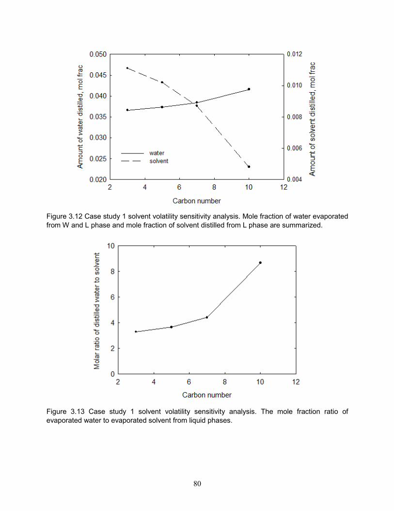
80

Figure 3.12 Case study 1 solvent volatility sensitivity analysis. Mole fraction of water evaporated

from W and L phase and mole fraction of solvent distilled from L phase are summarized.

Figure 3.13 Case study 1 solvent volatility sensitivity analysis. The mole fraction ratio of

evaporated water to evaporated solvent from liquid phases.

81

Figure 3.14 Case study 1 analytical Sor sensitivity to operation pressure.

Figure 3.15 Case study 1 operation pressure sensitivity analysis. Increased temperature during


82

Figure 3.16 Case study 1 operation pressure sensitivity analysis. Mole fraction of water

evaporated from W and L phase and mole fraction of solvent distilled from L phase are

summarized.

Figure 3.17 Case study 1 operation sensitivity analysis. The mole fraction ratio of evaporated

water to evaporated solvent from liquid phases is summarized with respect to carbon number.

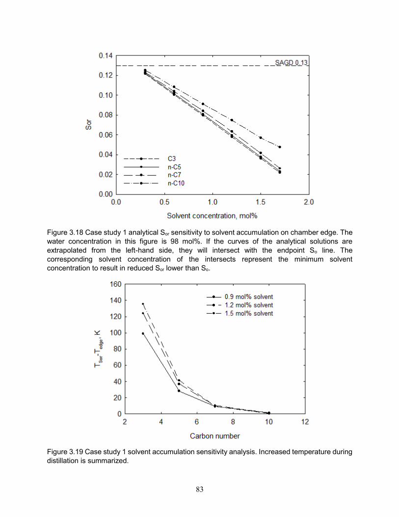
83

Figure 3.18 Case study 1 analytical Sor sensitivity to solvent accumulation on chamber edge. The

water concentration in this figure is 98 mol%. If the curves of the analytical solutions are

extrapolated from the left-hand side, they will intersect with the endpoint So line. The

corresponding solvent concentration of the intersects represent the minimum solvent

concentration to result in reduced Sor lower than So.

Figure 3.19 Case study 1 solvent accumulation sensitivity analysis. Increased temperature during


84

Figure 3.20 Case study 1 solvent accumulation sensitivity analysis. Mole fraction of water


summarized.

Figure 3.21 Case study 1 solvent accumulation analysis. The mole fraction ratio of evaporated

water to evaporated solvent from liquid phases is summarized with respect to carbon number.

85

Figure 3.22 Case study 1 analytical Sor sensitivity to water accumulation on chamber edge.

Figure 3.23 Case study 1 overall water concentration sensitivity analysis. Increased temperature

during distillation is summarized.

86

Figure 3.24 Case study 1 overall water concentration sensitivity analysis. Mole fraction of water


summarized.

Figure 3.25 Case study 1 overall water concentration analysis. The mole fraction ratio of

evaporated water to evaporated solvent from liquid phases is summarized with respect to carbon

number.

87


Figure 3.27 Case study 1 analytical Sor sensitivity to irreducible water saturation (Swr). Increased

temperature during distillation is summarized.

88

Figure 3.28 Case study 1 analytical Sor sensitivity to irreducible water saturation (Swr). Mole

fraction of water evaporated from W and L phase and mole fraction of solvent distilled from L

phase are summarized.

Figure 3.29 Case study 1 analytical Sor sensitivity to irreducible water saturation (Swr). The mole

fraction ratio of evaporated water to evaporated solvent from liquid phases is summarized with

respect to carbon number.

89

(1) n-C4

(2) n-C6

90

(3) n-C8

Figure 3.30 Case study 2 total molar enthalpy change with temperature. ΔT indicates temperature

range of solvent distillation. Ligter solvent has much larger temperature range.

(1) n-C4

91

(2) n-C6

(3) n-C8

Figure 3.31 Case study 2 analytical So changes with total molar enthalpy under 35 bars. C4 and

C6 are Ternary Type 1 while C8 is Ternary Type 2.

92

(1)

(2)

Figure 3.32 Simulation case study relative permeability curve.

93

Figure 3.33 Recovery factor for steam/n-alkane coinjection simulation case study. 2 mol% of solvent is coinjected with steam throughout the simulation. Type 2 solvents (C5, C7 and C10) can produce more bitumen faster than Type 1 solvent (C3).

Figure 3.34 Cumulative steam-oil ratio for steam/n-alkane coinjection simulation study. 2 mol% of solvent is coinjected with steam throughout the simulation. Type 2 solvents (C5 to C10) generally require less steam injection to recover same amount of bitumen as Ternary Type 1 (C3).

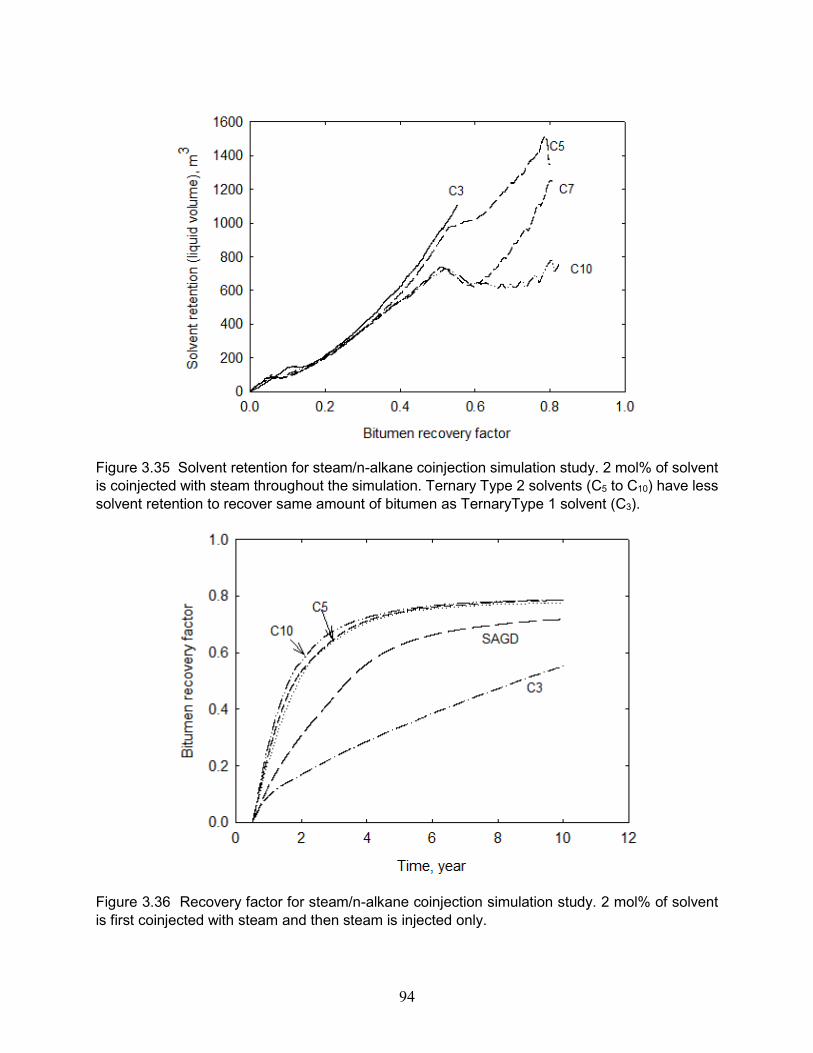
94

Figure 3.35 Solvent retention for steam/n-alkane coinjection simulation study. 2 mol% of solvent

is coinjected with steam throughout the simulation. Ternary Type 2 solvents (C5 to C10) have less

solvent retention to recover same amount of bitumen as TernaryType 1 solvent (C3).

Figure 3.36 Recovery factor for steam/n-alkane coinjection simulation study. 2 mol% of solvent

is first coinjected with steam and then steam is injected only.

95

Figure 3.37 Cumulative steam-oil ratio for steam/n-alkane coinjection simulation study. 2 mol%

of solvent is first coinjected with steam and then steam is injected only. C3 case is prolonged to

20 years.

Figure 3.38 Solvent retention for steam/n-alkane coinjection simulation study. 2 mol% of solvent

is first coinjected with steam and then steam is injected only. C3 case is prolonged to 20 years.

96

(1) Average oil saturation in reservoir at 35 bars

(2) Average oil saturation in reservoir at 60 bars

Figure 3.39 Qualitative validation of analytical solutions using simulation. Average oil saturation in reservoir is compared for 35 bars and 60 bars. At 35 bars, lighter solvents have better

97

displacement efficiency in the end. However, at 60 bars, the trend is not obvious, which is consistent with analytical prediction that all solvent essentially has almost the same Sor at 60 bars.

(1) C5

(2) C6

98

(3) C7

(4) C8

Figure 3.40 Qualitative validation of analytical solutions using simulation. Average oil saturation in reservoir w.r.t. pressure is examined. Lighter solvent has smaller differences in Sor change if pressure is increased from 35 to 60 bars. This is consistent with analytical solution predictions.

99

(1) Oil saturation profile

(2) Global concentration on the chamber edge for 12th row from the top

Figure 3.41 Qualitative validation of chamber edge overall composition impact on residual oil saturation. Lower solvent concentration and high water concentration on the chamber edge was found in the vicinity of the well pair, and therefore oil saturation is around 13%. However, deep inside the reservoir, solvent gradually accumulates and water concentration drops. Residual oil saturation correspondingly drops.

100

Figure 3.42 Qualitative validation of analytical solutions using simulation. Average oil saturation in reservoir w.r.t. Swr for n-C6 at 35 bars is examined. Swr affects Sor in a much more complicated way than just phase behavior. Endpoint Swr affects relative permeability curve and therefore affect flow in simulation.

101

Table 3.1 Conditions for the calculation of analytical Sor in sensitivity analysis for case study 1.

Case Solvent P, bars zsol, mol% zw,

mol% Swr Sor

Example calculation

n-C5 35 1.2 98 0.25 0.13

Volatility sensitivity C3, C5, C7, C10

35 1.2 98 0.25 0.13

Pressure sensitivity

C3, C5, C7, C10

15, 35, 60

1.2 98 0.25 0.13

zsol sensitivity C3, C5, C7, C10

35 0.9, 1.2, 1.5 98 0.25 0.13

zw sensitivity C3, C5, C7, C10

35 1:4 (bit/sol) - 0.10, 0.25,

0.40 0.13

Swr sensitivity C3, C5, C7, C10

35 1.2 98 0.25 0.13

Case study 2 C4, C6, C8 35 1:10

(bit/sol) 95 0.25 0.13

Table 3.2 Case study 1 example calculation. Beginning and ending temperature of n-C5 distillation and analytical residual saturations.

Tedge, K TSwr, K Swr Sor Sgr

n-C5 463.73 500.52 0.2497 0.0595 0.6907

Table 3.3 Case study 1 analytical residual oil saturation sensitivity to solvent volatility.


C3 374.68 498.77 0.2498 0.0579 0.6922

n-C5 463.73 500.52 0.2497 0.0595 0.6907

n-C7 492.85 503.07 0.2499 0.0633 0.6868

n-C10 507.67 508.50 0.2489 0.0747 0.6763

Table 3.4 Case study 1 analytical residual oil saturation sensitivity to operation pressure.

15 bars 35 bars 60 bars

Tedge, K TSwr, K Sor Tedge, K TSwr, K Sor Tedge, K TSwr, K Sor

C3 325.74 440.21 0.0589 374.68 498.77 0.0579 418.86 535.94 0.0578

n-C5 414.66 445.82 0.0612 463.73 500.52 0.0595 502.36 536.85 0.0592

n-C7 449.57 454.44 0.0674 492.85 503.07 0.0633 525.69 538.20 0.0620

n-C10 465.65 465.81 0.0818 507.67 508.50 0.0747 538.75 540.96 0.0701

102

Table 3.5 Case study 1 analytical residual oil saturation sensitivity to chamber edge solvent

concentration.

zsol,, mol% 0.3 0.6 0.9 1.2 1.5 1.7

C3 0.1214 0.1005 0.0794 0.0579 0.0363 0.0217

n-C5 0.1221 0.1017 0.0809 0.0595 0.0377 0.0231

n-C7 0.1230 0.1038 0.0840 0.0633 0.0415 0.0261

n-C10 0.1250 0.1082 0.0911 0.0747 0.0570 0.0475

Table 3.6 Case study 1 analytical residual oil saturation sensitivity to chamber edge global water

concentration.

zw, mol% C3 n-C5 n-C7 n-C10

99 0.0139 0.0142 0.0149 0.0178

98 0.029 0.0303 0.034 0.0525

97 0.0449 0.0481 0.0586 0.0888

96 0.0617 0.0685 0.0883 0.1227

95 0.0799 0.092 0.1212 -

94 0.0999 0.1188 - -

93 0.1231 - - -

Table 3.7 Case study 1 analytical residual oil saturation sensitivity to irreducible water saturation

(Swr).

Swr C3 n-C5 n-C7 n-C10

0.10 0.0248 0.0251 0.0257 0.0279

0.25 0.0579 0.0595 0.0633 0.0747

0.40 0.0936 0.0985 0.1083 0.1264

Table 3.8 Case study 2 analytical residual oil saturation.


n-C4 416.00 446.66 0.2500 0.0259 0.7241

n-C6 474.33 477.10 0.2498 0.0486 0.7015

n-C8 497.03 497.42 0.2491 0.0874 0.6634

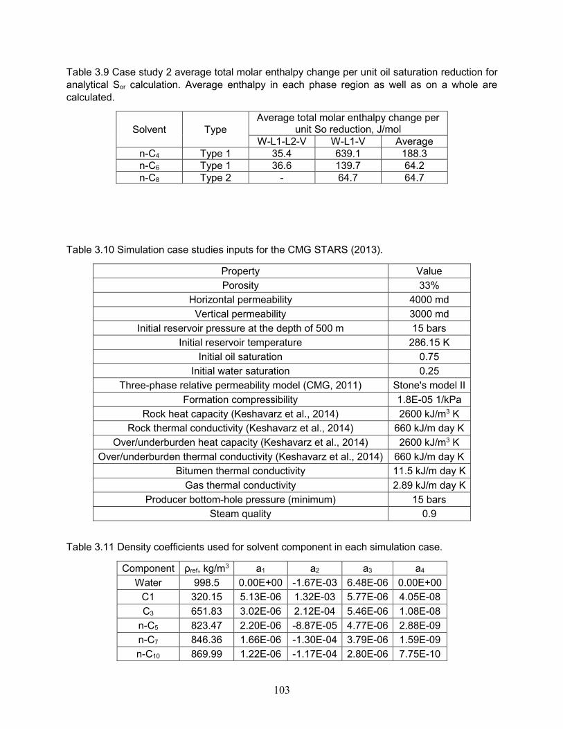
103

Table 3.9 Case study 2 average total molar enthalpy change per unit oil saturation reduction for

analytical Sor calculation. Average enthalpy in each phase region as well as on a whole are

calculated.

Solvent Type

Average total molar enthalpy change per unit So reduction, J/mol

W-L1-L2-V W-L1-V Average

n-C4 Type 1 35.4 639.1 188.3

n-C6 Type 1 36.6 139.7 64.2

n-C8 Type 2 - 64.7 64.7

Table 3.10 Simulation case studies inputs for the CMG STARS (2013).

Property Value

Porosity 33%

Horizontal permeability 4000 md

Vertical permeability 3000 md

Initial reservoir pressure at the depth of 500 m 15 bars

Initial reservoir temperature 286.15 K

Initial oil saturation 0.75

Initial water saturation 0.25

Three-phase relative permeability model (CMG, 2011) Stone's model II

Formation compressibility 1.8E-05 1/kPa

Rock heat capacity (Keshavarz et al., 2014) 2600 kJ/m3 K

Rock thermal conductivity (Keshavarz et al., 2014) 660 kJ/m day K

Over/underburden heat capacity (Keshavarz et al., 2014) 2600 kJ/m3 K

Over/underburden thermal conductivity (Keshavarz et al., 2014) 660 kJ/m day K

Bitumen thermal conductivity 11.5 kJ/m day K

Gas thermal conductivity 2.89 kJ/m day K

Producer bottom-hole pressure (minimum) 15 bars

Steam quality 0.9

Table 3.11 Density coefficients used for solvent component in each simulation case.

Component ρref, kg/m3 a1 a2 a3 a4

Water 998.5 0.00E+00 -1.67E-03 6.48E-06 0.00E+00

C1 320.15 5.13E-06 1.32E-03 5.77E-06 4.05E-08

C3 651.83 3.02E-06 2.12E-04 5.46E-06 1.08E-08

n-C5 823.47 2.20E-06 -8.87E-05 4.77E-06 2.88E-09

n-C7 846.36 1.66E-06 -1.30E-04 3.79E-06 1.59E-09

n-C10 869.99 1.22E-06 -1.17E-04 2.80E-06 7.75E-10

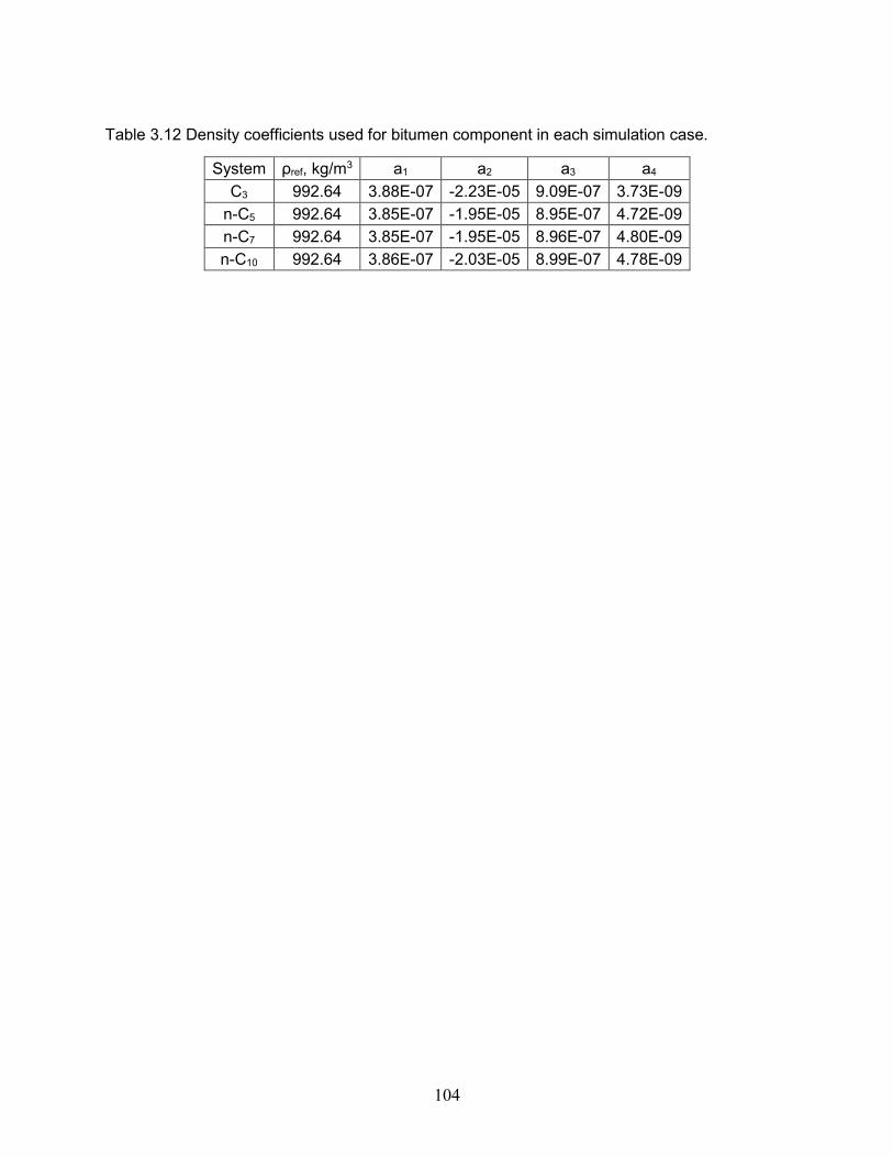
104

Table 3.12 Density coefficients used for bitumen component in each simulation case.

System ρref, kg/m3 a1 a2 a3 a4

C3 992.64 3.88E-07 -2.23E-05 9.09E-07 3.73E-09

n-C5 992.64 3.85E-07 -1.95E-05 8.95E-07 4.72E-09

n-C7 992.64 3.85E-07 -1.95E-05 8.96E-07 4.80E-09

n-C10 992.64 3.86E-07 -2.03E-05 8.99E-07 4.78E-09

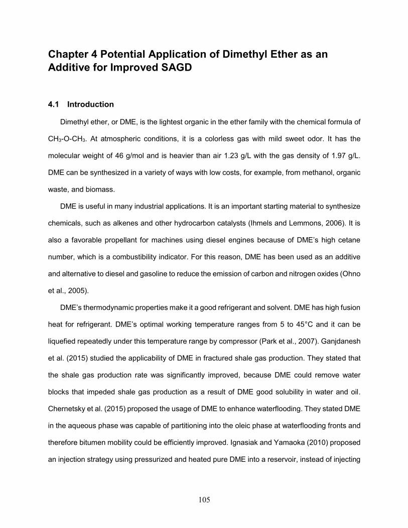
105

Chapter 4 Potential Application of Dimethyl Ether as an

Additive for Improved SAGD

4.1 Introduction

Dimethyl ether, or DME, is the lightest organic in the ether family with the chemical formula of

CH3-O-CH3. At atmospheric conditions, it is a colorless gas with mild sweet odor. It has the

molecular weight of 46 g/mol and is heavier than air 1.23 g/L with the gas density of 1.97 g/L.

DME can be synthesized in a variety of ways with low costs, for example, from methanol, organic

waste, and biomass.

DME is useful in many industrial applications. It is an important starting material to synthesize

chemicals, such as alkenes and other hydrocarbon catalysts (Ihmels and Lemmons, 2006). It is

also a favorable propellant for machines using diesel engines because of DME’s high cetane

number, which is a combustibility indicator. For this reason, DME has been used as an additive

and alternative to diesel and gasoline to reduce the emission of carbon and nitrogen oxides (Ohno

et al., 2005).

DME’s thermodynamic properties make it a good refrigerant and solvent. DME has high fusion

heat for refrigerant. DME’s optimal working temperature ranges from 5 to 45°C and it can be

liquefied repeatedly under this temperature range by compressor (Park et al., 2007). Ganjdanesh

et al. (2015) studied the applicability of DME in fractured shale gas production. They stated that

the shale gas production rate was significantly improved, because DME could remove water

blocks that impeded shale gas production as a result of DME good solubility in water and oil.

Chernetsky et al. (2015) proposed the usage of DME to enhance waterflooding. They stated DME

in the aqueous phase was capable of partitioning into the oleic phase at waterflooding fronts and

therefore bitumen mobility could be efficiently improved. Ignasiak and Yamaoka (2010) proposed

an injection strategy using pressurized and heated pure DME into a reservoir, instead of injecting

106

steam as in SAGD or CSS. They stated that the latent heat released by DME condensation as

well as DME dissolution into bitumen could effectively reduce bitumen viscosity. They further

stated DME can be recycled from produced bitumen and reinjected into reservoir. However, the

applicability of steam-DME coinjection is not yet discussed in the literature.

Chapter 3 presented through analytical solutions the solvent distillation effect on

displacement efficiency. C3 has the potential to achieve the greatest displacement efficiency

because of its high volatility. However, it requires much more temperature increase to fulfill its

potential than heavier n-alkanes that tend to exhibit narrow-boiling behavior. Therefore, a

desirable solvent in terms of the distillation mechanism would be as volatile as C3, but should

require a smaller increase in temperature to achieve low Sor.

Although the vapor pressures of DME and C3 are similar to each other, their solubilities in the

aqueous phase are quite different. This indicates that the interaction of DME with water is

substantially different from that of C3 with water. For example, experimental data show that the

three-phase PT curve for water/DME is on the higher-temperature side of that for water/C3 (Pozo

and Streett, 1984), as will be discussed in this chapter. Therefore, steam-DME coinjection may

result in higher operating temperatures than coinjection of other hydrocarbon solvents with similar

volatility, such as C3. The three-phase PT curve for a water/solvent binary is a good approximation

for the lower bound for chamber-edge temperature when that solvent is coinjected with steam

(Chapter 2).

For this reason, this chapter investigates the potential of DME as an additive for improved

SAGD in terms of operating temperature distribution, which affects the gravity drainage rate of oil,

steam requirement, and residual oil. Also, the DME injected can be recovered through the

aqueous and oleic phases, unlike conventional hydrocarbons solvents that can only be recovered

from the oleic phase. In the subsequent sections, phase behavior prediction of the

water/bitumen/DME system is studied based on an EOS. Then, steam/DME coinjection is

discussed via both analytical solution and numerical simulation. Its performance is compared with

107

n-alkane solvents in terms of energy efficiency and solvent retention. A simple economic analysis

will be also presented.

4.2 Phase Behavior of Water/Bitumen/DME Mixtures

4.2.1 EOS Model

In this research, the PR EOS with the vdW mixing rules is used because only simple cubic

EOSs, such as the PR EOS, are implemented in the commercial software to be used in this

chapter. In order to more accurately describe phase behavior of DME-containing systems,

however, it is desirable to use more advanced EOS and/or mixing rules, such as Wong and

Sandler mixing rules (Wong and Sandler, 1992; Tallon and Fenton, 2010).

Only three components are considered in the system, water, DME, and the bitumen

characterized as one pseudo component as described in Chapter 2. Critical properties of DME

were experimentally determined by Tallon and Fenton (2006). The critical properties and acentric

factors for the three components are summarized in Table 4.1.

The BIP correlation between water and bitumen remains the same as described in Chapter

2. However, due to limited BIP information between DME and other components, data from

available publications and their reliability against experimental data are inspected. Here,

Ganjdanesh et al.’s (2015) BIPs for water/DME and bitumen/DME are examined and calibrated

to match experiments, as summarized in Table 4.2. Details of the calibration are explained below.

EOS predictions are compared with experimental data (Pozo and Streett, 1984) in terms of

vapor-liquid-liquid equilibrium (VLLE) for the water/DME binary. They measured VLLE P-T data

from 10 to 60 bars (Table 4.3), which caters to the operation range of SAGD and its variants.

Both three-phase P-T curve and DME dissolution in the aqueous phase are considered for the

calibration of the PR-EOS model. Average absolute relative deviation (AARD) in percentage and

108

average absolute deviation (AAD) are calculated and summarized in Table 4.6. AARD and AAD

are defined as follows,

AARD =1

𝑛∑ |

𝑥𝐸𝑂𝑆 − 𝑥𝐸𝑋𝑃

𝑥𝐸𝑋𝑃|

𝑛

𝑖=1

(4.1)

AAD =1

𝑛∑ |𝑥𝐸𝑂𝑆 − 𝑥𝐸𝑋𝑃|

𝑛

𝑖=1

(4.2)

where xEOS is an EOS predicted value, xEXP experiment determined value, and n is the number of

experiment data.

For the water/DME system, the PR EOS and the vdW mixing rules have limited ability to

predict phase behavior, because the vdW mixing rules are not accurate for highly non-ideal

mixtures such as water/DME solution. The BIP of -0.17 is the optimal value for the PR EOS with

the vdW mixing rules. This BIP gives reasonably accurate predictions for water/DME three-phase

P-T curve and DME solubility in water. As mentioned earlier, matching DME solubility in water is

important because the distillation analysis indicates that a water-soluble solvent may increase

chamber edge temperature.

By using the P3p in Table 4.3, T3p attained by EOS is compared with the corresponding

experimental data. From 10 to 60 bars, AARD of EOS prediction is 4.91% and AAD is 19.92 K.

AARD and AAD of EOS prediction at 35 bars is 3.83% and 14.8 K.

DME solubility in the aqueous phase is compared between EOS and experiment at three-

phase conditions, by using the P3p in Table 4.3. DME solubility from 10 to 60 bars predicted by

the PR-EOS model with this BIP is on the same order of magnitude as experimental data. AARD

of EOS prediction is 40.74% and AAD is 6.58 mol%. At 35 bars, EOS gives estimated 55% AARD

and 4.5 mol% AAD.

Figure 4.1 shows deviations of EOS predictions from experiment data. In terms of three-

phase curve, the EOS model generally gives overestimated values. In terms of DME solubility in

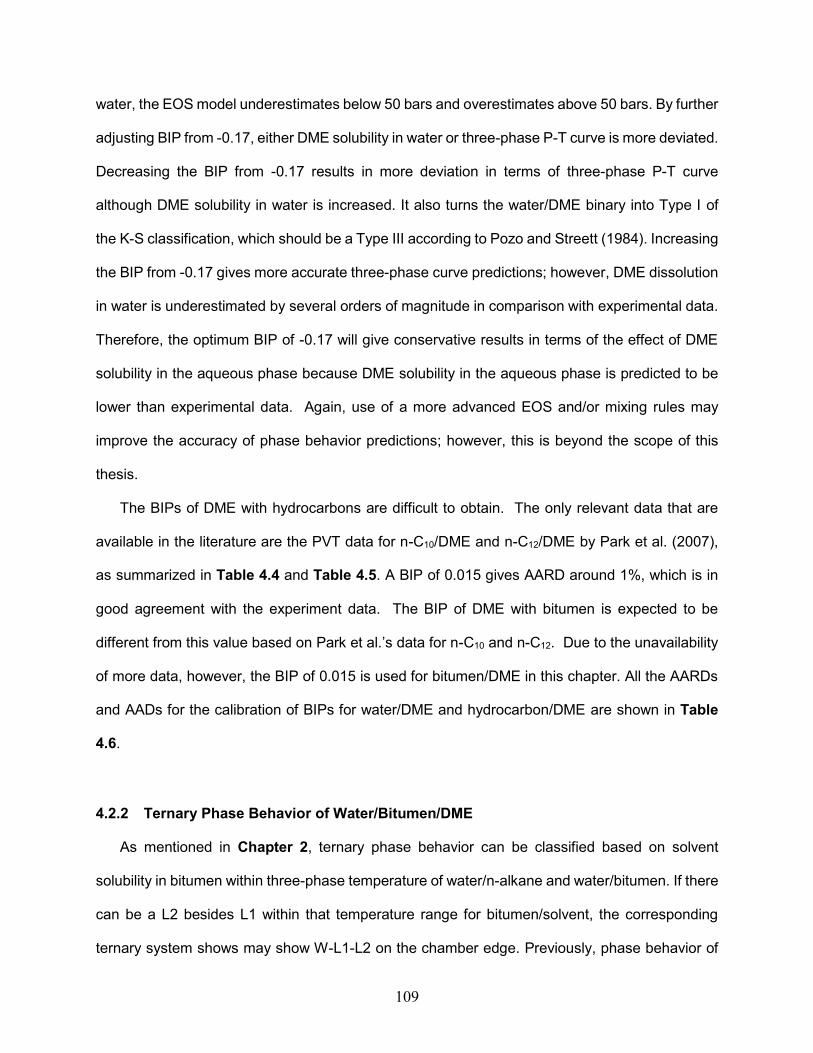
109

water, the EOS model underestimates below 50 bars and overestimates above 50 bars. By further

adjusting BIP from -0.17, either DME solubility in water or three-phase P-T curve is more deviated.

Decreasing the BIP from -0.17 results in more deviation in terms of three-phase P-T curve

although DME solubility in water is increased. It also turns the water/DME binary into Type I of

the K-S classification, which should be a Type III according to Pozo and Streett (1984). Increasing

the BIP from -0.17 gives more accurate three-phase curve predictions; however, DME dissolution

in water is underestimated by several orders of magnitude in comparison with experimental data.

Therefore, the optimum BIP of -0.17 will give conservative results in terms of the effect of DME

solubility in the aqueous phase because DME solubility in the aqueous phase is predicted to be

lower than experimental data. Again, use of a more advanced EOS and/or mixing rules may

improve the accuracy of phase behavior predictions; however, this is beyond the scope of this

thesis.

The BIPs of DME with hydrocarbons are difficult to obtain. The only relevant data that are

available in the literature are the PVT data for n-C10/DME and n-C12/DME by Park et al. (2007),

as summarized in Table 4.4 and Table 4.5. A BIP of 0.015 gives AARD around 1%, which is in

good agreement with the experiment data. The BIP of DME with bitumen is expected to be

different from this value based on Park et al.’s data for n-C10 and n-C12. Due to the unavailability

of more data, however, the BIP of 0.015 is used for bitumen/DME in this chapter. All the AARDs

and AADs for the calibration of BIPs for water/DME and hydrocarbon/DME are shown in Table

4.6.

4.2.2 Ternary Phase Behavior of Water/Bitumen/DME

As mentioned in Chapter 2, ternary phase behavior can be classified based on solvent

solubility in bitumen within three-phase temperature of water/n-alkane and water/bitumen. If there

can be a L2 besides L1 within that temperature range for bitumen/solvent, the corresponding

ternary system shows may show W-L1-L2 on the chamber edge. Previously, phase behavior of

110

water/bitumen/n-alkane system was studied based on bitumen/n-alkane binary behavior.

Bitumen/n-alkane is a Type IIIm binary of the K-S classification. At T3p of water/n-alkane,

bitumen/n-alkane always shows L1 one phase or L1-L2 two phases. Therefore, the existence of

phase boundaries between two-phase regions of oil/solvent binary within coinjection operation

temperature range determines classification of corresponding ternary systems. Two ternary types

are classified based on whether L1 or L2 can coexists within the steam-solvent coinjection

temperature range.

DME-containing reservoir fluids can be classified by following the same logic. For the

water/bitumen/DME system described in §4.2.1, bitumen/DME is a Type IIIm of the K-S

classification. See Figure 4.2 for vapor pressure curves and three-phase curve of

water/bitumen/DME system. The volatility of DME is between C3 and n-C4. Also see Table 4.7 for

comparison of binary pairs for n-alkane containing system and DME containing system. It would

be interesting to see the phase behavior of bitumen/DME binary at the three-phase temperature

of water/DME at a specific pressure to see the corresponding water/bitumen/DME ternary

classification.

Figure 4.3 shows T-x diagrams at 35 bars for water/DME and bitumen/DME. (1) Water/DME

at 35 bars shows similar T-x diagram as water/n-alkane. Unlike water/n-alkane, three-phase line

of water/DME is to the right of DME vapor curve so that three-phase temperature in Figure 4.3

(1) is higher than DME saturated temperature. In contrast, three-phase temperature of water/n-

alkane is always lower than n-alkane saturated temperature. (2) Since there is not L2 within the

temperature range for bitumen/DME, the corresponding ternary system should show Ternary

Type 2 behavior on the chamber edge.

Figure 4.4 demonstrates ternary phase behavior of water/bitumen/DME at 35 bars. In (1) and

(2), when temperature is low, only W-L1-L2 three-phase region exists. In (3), a second three-

phase region, V-L1-L2 starts to coexist with W-L1-L2 when temperature is greater than saturated

temperature of DME. In (4) and (5), complex three-phase transition happens. L2 exists when

111

temperature is equal to or lower than three-phase temperature of water/DME. W-L1-L2 merges

with V-L1-L2 into W-L1-V as temperature increases. L2 disappears the instant two three-phase

regions merge. From (6) to (8), as temperature keeps increasing, L1 swings towards

water/bitumen edge, as n-alkane systems, and finally three-phase regions disappears onto

water/bitumen edge. As can be seen that, W-L1-L2 is only possible below the lowest temperature

bound, the three-phase temperature of water/DME. This is a Ternary Type 2 system.

Much higher DME solubility in water compared to n-alkanes may be beneficial in steam-

solvent coinjection. Figure 4.5 shows ternary diagrams at the chamber edge conditions for water-

soluble solvents like DME and water-insoluble solvents like n-alkane. The operation pressure is

35 bars, and global water concentration on the chamber edge is 95 mol% and solvent

concentration is 4 mol%. DME case has higher chamber edge temperature than Ternary Type 1

n-alkane cases, however lower than Ternary Type 2 n-alkane cases. For the same overall

composition on a chamber edge, the L vertex of W-L-V for water-soluble solvent case is closer to

the water/bitumen edge, which gives a higher chamber-edge temperature than when the solvent

is insoluble in water. The following sections will provide a more detailed study of increased

chamber-edge temperature.

4.3 Steam/DME coinjection

In this section, coinjection of DME with steam into a bitumen reservoir is numerically studied.

Firstly, the algorithm developed in Chapter 3 for residual oil saturation after distillation is applied

to steam-DME coinjection. Then, steam-DME coinjection is simulated with the CMG STARS

simulator (Computer Modelling Group Ltd., 2013). Its performance is compared with n-alkanes in

terms of energy efficiency and economic performance.

112

4.3.1 Liquid DME Density

Before performing the analytical solution to estimate the distillation effect on residual oil

saturation, it is important to obtain a reliable density model for liquid DME. Modified Rackett

equations were used by Ihmels and Lemmon (2006) for accurate representation of liquid DME

density from 10 to 400 bars and 273 to 523 K. The liquid density prediction of this model gives

0.039% AARD from experimental data. The modified Rackett equations are,

𝜌 =𝜌0

[1 − 𝐶𝑇ln ((𝐵𝑇 + 𝑃)/(𝐵𝑇 + 𝑃0))] (4.2)

𝜌0 =𝐴𝑅

𝐵𝑅[1+(1−

𝑇𝐶𝑅

)]𝐷𝑅 (4.3)

𝐵𝑇 = 𝐵𝑇0 + 𝐵𝑇1

𝑇

𝐸𝑇+ 𝐵𝑇2(

𝑇

𝐸𝑇)2 (4.4)

where ρ is the liquid density of DME, CT=0.0834042, BT0=284.304, BT1=-130.021, BT2=14.4194,

ET=100, AR=55.6001, BR=0.236704, CR=401.406 and DR=0.243368. The CMG STARS simulator

uses the liquid density model described in Appendix B, instead of Rackett ones. Therefore, the

model was regressed to match Rackett’s model by adjusting the five parameters, 𝜌𝑖𝑟𝑒𝑓 and α1 to

α4. The regression results have an R-square index of 0.9998, and are given in Table 4.8.

4.3.2 Liquid DME Viscosity Model

Steam-solvent coinjection reduces bitumen viscosity by solvent dilution and steam latent heat.

In numerical simulation, viscosity has to be reasonably modeled.

CMG STARS (Computer Modelling Group Ltd., 2013) using logarithmic linear or non-linear

mixing of pure component viscosities for oleic phase viscosity. Non-linear logarithmic mixing is

recommended because viscosity of bitumen and volatile solvent mixture is highly non-linear to

solvent concentration in bitumen (Venkatramani and Okuno, 2016).

113

The saturated liquid DME viscosity correlation developed by Wu et al. (2003) is used to

generate viscosity-temperature table at DME subcritical conditions for STARS. The correlation is

as follows:

log10 𝜇 = −5.7282 +631.031

𝑇+ 0.01453𝑇 + 1.8225 × 10−5𝑇2 (4.5)

where μ is viscosity in mPa∙s and T is temperature in K. This correlation gives 0.5% AARD to the

experimental data measured from 227 to 343 K. DME becomes supercritical at temperatures

greater than 427.4 K. However, supercritical DME viscosity data has not yet been measured to

my knowledge. Supercritical viscosity of C4 is used in this research for DME under supercritical

conditions. Comparison of viscosity-temperature curves between n-alkanes and DME are shown

in Figure 4.6. DME shows similar viscosity to n-C4. However, DME viscosity is not as sensitive to

temperature as n-C4. DME is more viscous than n-C4 if temperature is greater than 400 K.

In the absence of experimental viscosity data for water/DME and bitumen/DME mixtures, a

sensitivity analysis should be done in terms of the coefficients used for the non-linear logarithmic

mixing rule. In the simulation case study in §4.3.4, viscosity mixing coefficients of C4 are used for

DME. Then §4.3.5, a sensitivity analysis is conducted on the impact of viscosity model on

simulation results. Details of how non-linear coefficients are obtained for bitumen and n-alkanes

can be found in the research of Venkatramani and Okuno (2016).

4.3.3 Analytical Solution Study

The algorithm for analytical Sor is performed with the PR-EOS model presented in §4.2.1.

Liquid density model for water and bitumen is the same as in Chapter 3. The liquid density model

for DME in §4.3.1 is used.

Figure 4.7 shows the result of DME comparison with C3 in terms of Sor under the condition of

35 bars, the overall water concentration of 98 mol% and the Swr of 0.25. A number of overall

solvent concentrations on the chamber edge were used to get a series of calculated Sor. Results

114

show that DME is only slightly better than C3 to reduce oil saturation due to distillation effect.

Besides, DME and C3 show a similar sensitivity of the calculated Sor to the overall solvent

accumulation on the chamber edge.

In Chapter 2, it was shown that C3 has the greatest potential to reduce Sor among the solvents

studied. However, several disadvantages of C3 greatly impede its potential, such as low chamber

edge temperature, poor solvent mixing because of oleic-phase separation, and a large

temperature increase to achieve Sor. By investigation of the distillation process of DME, Figure

4.8 shows the beginning and the end of the distillation process by demonstration of ternary phase

diagrams on the chamber edge and at the temperature of lowest oil saturation. The L-phase

composition does not change much during the distillation. However, the chamber-edge

temperature is so much increased because of the DME solubility in water. Figure 4.9 shows So

reduction comparison between C3 and DME during distillation. The temperature at which

distillation starts (Tedge) for DME is much higher than that of C3 for the conditions examined. The

incremental temperature (ΔT), i.e. TSwr-Tedge, for distillation of DME is much smaller than that of

C3. At 35 bars with 98 mol% overall water, 1.2 mol% solvent and 0.25 Swr (Figure 4.8), the C3

case needs a temperature increase of 124.9 K to achieve the Sor of 0.058, while DME only needs

the temperature increase of 8.6 K to achieve a similar Sor of 0.056.

Figure 4.10 and Figure 4.11 show the ΔT of the DME case compared to n-alkanes as well

as water and DME distillation compared to n-alkanes. 4.2 mol% of water evaporates in the DME

case, almost the same as the amount of water evaporated in C10 case. 0.6 mol% of DME

evaporates from the L phase, which is less than C8 but more than C10. More water evaporates

from liquid phases than light n-alkanes with smaller ΔT. Because of the DME partitioning inside

the W phase, DME can evaporates from both the W and L phases during distillation. DME’s

enhanced displacement efficiency is different from n-alkanes in that the volume shrinkage of the

L phase is a result of both solvent distillation from the L phase and water evaporation from the W

phase. In DME case, however, what may make DME good in displacement efficiency is primarily

115

the aqueous phase evaporation that minimizes oleic phase saturation. The DME evaporated from

the aqueous phase makes the aqueous phase more volatile.

Figure 4.12 shows water and solvent evaporated from both aqueous and oleic phases during

distillation for the DME and n-alkane cases. For increased solvent accumulation, the water

evaporated is not much affected. The increased ΔT and DME distillation accounts for extra oil

saturation reduction.

Besides solvent accumulation, sensitivity analysis is also done for pressure, chamber edge

water concentration and endpoint water saturation of reservoir. All the explanations of enhanced

displacement efficiency resemble the ones shown in Figure 4.10 to Figure 4.12.

In Figure 4.13, three different pressures, 15, 35 and 60 bars, are used to calculate residual

oil saturation analytical solutions while global water concentration, solvent concentration and Swr

remain 98 mol%, 1.2 mol% and 0.25 respectively. Unlike heavier n-alkane solvents such as C7 of

which Sor can be significantly decreased by increasing operation pressure, DME has very similar

sensitivity to pressure as C3. For both DME and C3, Sor does not vary much with pressure change.

Increased pressure generally increases the ΔT of DME. Also, solvent distillation is more

pronounced if pressure is higher. DME has limited capacity to further distill solvent, just like C3.

In Figure 4.14, sensitivity of Sor to chamber edge water concentration is shown. Pressure,

solvent concentration and Swr are set to 35 bars, 1.2 mol% and 0.25 respectively. Again, due to

similar volatility, DME and C3 have similar sensitivity to water concentration. 1 mol% of water

increase results in significant oil saturation reduction, mainly because of lowered chamber edge

oil saturation.

In Figure 4.15, sensitivity of analytical Sor to endpoint water saturation is shown. Pressure is

set to 35 bars. Water and solvent concentration on chamber edge are 98 and 1.2 mol%

respectively. Analytical Sor decreases as Swr decreases. Same as other n-alkane solvents, DME

distillation can be more profound for reservoirs with lower residual water saturation as a result of

increased ΔT.

116

4.3.4 Comparison between DME and n-alkanes

This section presents the comparison between DME and n-alkanes in steam/solvent

coinjection through simulation studies. The solvent efficiency, which is measured by bitumen

recovery, SOR, and solvent retention, is first compared. Then, a simple economic analysis is

presented.

A single-sided reservoir model is used as described for n-alkanes in §3.5 to compare DME

and n-alkanes in terms of bitumen recovery, SOR, and solvent retention. All other reservoir

parameters and operation conditions are the same as in Chapter 3. At 35 bars, 2 mol% of solvent

is coinjected with steam until the steam chamber reaches the outer reservoir boundary.

Figure 4.16 compares DME with n-alkanes in terms of bitumen-recovery predictions. The

DME case can produce bitumen faster than C3 (Ternary Type 1) and achieve the bitumen

recovery that is close to those with light n-alkanes within Ternary Type 2 by the end of production.

As explained by analytical solutions in §4.2.2, improved chamber-edge conditions because of

water dissolution may account for improved drainage rate compared to C3. However, bitumen

drainage rate of the water-DME coinjection case is similar to SAGD. This can be a result of

underestimated chamber-edge temperature in this simulation, due to the underestimated DME

solubility in the aqueous phase by use of the EOS model. The DME solubility in water predicted

by the EOS model is only half of what was observed in the experiment of Pozo and Streett (1984).

Figure 4.16 also shows that the ultimate recovery is higher for the DME case than the SAGD case

because of enhanced displacement efficiency in the DME case.

In Figure 4.17, the temperature profiles in the simulated reservoir are compared among C3,

DME and C5 when the same amount of bitumen was recovered. C3 has the lowest inside-chamber

temperature. DME and heavy n-alkanes have higher inside-chamber temperature. Ternary Type

2 solvents require less temperature increase to achieve Sor. C3 may take longer time to achieve

its highest temperature and lowest Sor.

117

The chamber-edge conditions are now examined in simulation. Figure 4.18 compares the

temperature distribution between DME and selected n-alkanes near a chamber edge. At 35 bars,

DME shows an increased chamber-edge temperature than C3 and C4. This increased chamber-

edge temperature is a result of the DME solubility in the aqueous phase and the three-phase

temperature of water/DME that is higher than the DME condensation temperature at the pressure

of interest. The L phase in the DME case has higher bitumen-to-solvent ratio than C3 and C5.

However, DME still has lower chamber-edge temperature than C5. As mentioned before, DME

solubility is underestimated with the current PR-EOS model; therefore, a chamber-edge

temperature for the DME case can be underestimated as well. Figure 4.19 and Figure 4.20

compare DME with selected n-alkanes in terms of the L1-phase composition near a chamber

edge. The increased chamber-edge temperature in the DME case results in the DME

concentration in the L1 phase that is similar to the C3 case, but a higher concentration of water

than the C4 case.

Figure 4.21 and Figure 4.22 compares the DME and n-alkane cases in terms of CSOR and

solvent retention, respectively. For both DME and n-alkane cases, solvent retention first reaches

a highest level, and then declines as only steam is injected when steam chamber reaches the

outer reservoir boundary. In terms of the highest level of solvent retention, the DME case is the

lowest. The DME case exhibits a similar or even lower CSOR and solvent retention as Ternary

Type 2 solvents; however, DME is cheaper than Ternary Type 2 n-alkanes according to the data

source referenced in this research. Figure 4.23 shows the production (or recovery) of DME. Due

to the solubility of DME in the aqueous and oleic phases at reservoir conditions, DME can be

recovered by the flow of the aqueous and oleic phases. In contrast, n-alkanes can be recovered

only by the flowing oleic phase.

DME is likely cheaper than heavy Ternary Type 2 n-alkanes. A simple economic analysis is

presented to show the economic potential of the use of DME as an additive to steam. A reservoir

with dimensions of 142×500×20 (m) is divided into 71×1×20 gridblocks. The well length is 500 m

118

and horizontal well pair is placed as shown in Figure 4.24. Other reservoir simulation parameters

are the same as aforementioned single-sided reservoir in Chapter 3. Solvent injection is ceased

immediately after steam chamber reaches the outer reservoir boundary. Table 4.9 summarizes

time when chamber edge reaches reservoir boundary for each case. Net present value (NPV) is

calculated for DME and n-alkane solvents (Table 4.10). Bitumen price is an average reference

price from January 2015 to February 2016 of Alberta provincial government statistics. Due to the

lack of latest solvent prices in the literature, solvent prices in the market for industrial usage

purposes are used. The solvent prices are roughly averaged from December 2015 to April 2016.

The formulation for NPV and other inputs refer to Keshavarz et al. (2015). The formulation is

shown below.

Net Present Value (NPV) [USD] = (cumulative oil × oil price) × (1.0 – discount rate) [USD]

– capital cost of exploration

– capital cost of well pair [USD]

– water treatment equipment [USD]

– steam generator cost [USD]

– capital cost of solvent distribution [USD]

– administration and head office [USD]

– blending and transportation [USD]

– production years × well pair and field operation [USD/year]

– production years × solvent handling [USD/year]

– cumulative steam injection [m3 CWE] × (generator

operation [USD/m3 CWE] + fuel cost [USD/m3 CWE])

– cumulative water production [m3] × treatment of production

water [USD/m3]

– (cumulative solvent injection [m3] – cumulative solvent

production [m3]) × solvent price [USD/m3]

119

(4.6)

Figure 4.25 compares NPVs for the DME and n-alkane cases. Maximum NPV and the time

for the maximum achieved for each case are summarized in Table 3.2, which indicates when the

project should stop. C10 has the highest maximum NPV, followed by DME, C7, SAGD, C5 and C3.

For the C10 case, a deficit is expected for the first several years, and later on the project starts to

make profit by recycling C10 via steam-only injection. The time that the maximum NPV is achieved

could be numerically simulated, but it may be risky to use C10 considering the substantial

importance of recovering C10 for achieving the highest NPV. Although Ternary Type 2 solvents

produce bitumen faster early in the process, the loss of expensive n-alkanes may totally counter

the advantages of Ternary Type 2 solvents. N-alkane cases are only more profitable than SAGD

if solvents can be effectively recycled. In contrast, the DME case makes profit steadily before the

chamber edge reaches the outer reservoir boundary. Although it is making profits slower than

SAGD in the beginning, it results in a higher maximum NPV than SAGD and most n-alkanes

cases. Therefore, if making profit quickly at a lower risk is the objective, DME and light Ternary

Type 2 solvents can be good choices of solvent to be coinjected with steam. Under a higher oil-

price environment, the advantage of steam-solvent coinjection over SAGD may be more

pronounced.

Around 4.3 years, the DME case reaches the reservoir boundary. Steam-only injection helps

further improve the profit by recycling DME from the water and oleic phases by increasing

temperature, as was illustrated previously in Figure 4.22. Further, the NPV of the DME case is

less sensitive to the injection strategy change compared to heavy Ternary Type 2 solvents such

as C10, i.e., there is no obvious turning point in the NPV curve for the DME case when solvent

injection is stopped. There is a good reason for this. The distillation of C10 requires less ΔT, and

is more sensitive to overall water concentration as illustrated in Chapter 3. It is important to

recover expensive solvent like C10 by stopping injecting solvent to make ES-SAGD profitable. The

120

indication behind this is that, it can be economically beneficial if a solvent like DME is used that

is less expensive, easier to recover from the reservoir, and efficient to produce bitumen.

4.3.5 Sensitivity of DME Simulation Results to Viscosity Model

Since no data is available for viscosities of DME containing mixtures, a sensitivity analysis is

performed for the viscosity models used in simulation to show how viscosity modelling can affect

simulation results. The DME-saturated liquid viscosity mentioned in §4.3.2 with the mixing

coefficients of C3, C4 and C5 for bitumen/DME mixture viscosity is used as in Venkatramani and

Okuno (2016). Also, viscosity of C3, C4 and C5 are used for DME are used as well with C4

coefficients.

Five sets of viscosity models are used for DME simulation. Their bitumen recovery at the first

five years and average bitumen drainage rate are compared with that of SAGD. Here, single-

sided reservoir as described in Section 3.5 is used. Steam and solvent are coinjected throughout

the simulation. Five sets of viscosity models are:

(1) DME saturated liquid viscosity in §4.3.2 and non-linear logarithmic mixing coefficients of

C3 for oleic phase;


C4 for oleic phase;


C5 for oleic phase;

(4) C4 saturated liquid viscosity and non-linear logarithmic mixing coefficients of C3 for oleic

phase; and

(5) C4 saturated liquid viscosity and non-linear logarithmic mixing coefficients of C5 for oleic

phase.

Figure 4.26 shows bitumen recovery for the first five years. Figure 4.27 shows average

bitumen drainage rate at 4 years for each case. In general, if C3 viscosity and/or mixing

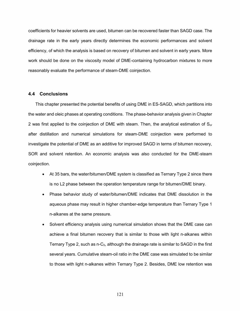
121

coefficients for heavier solvents are used, bitumen can be recovered faster than SAGD case. The

drainage rate in the early years directly determines the economic performances and solvent

efficiency, of which the analysis is based on recovery of bitumen and solvent in early years. More

work should be done on the viscosity model of DME-containing hydrocarbon mixtures to more

reasonably evaluate the performance of steam-DME coinjection.

4.4 Conclusions

This chapter presented the potential benefits of using DME in ES-SAGD, which partitions into

the water and oleic phases at operating conditions. The phase-behavior analysis given in Chapter

2 was first applied to the coinjection of DME with steam. Then, the analytical estimation of Sor

after distillation and numerical simulations for steam-DME coinjection were performed to

investigate the potential of DME as an additive for improved SAGD in terms of bitumen recovery,

SOR and solvent retention. An economic analysis was also conducted for the DME-steam

coinjection.

At 35 bars, the water/bitumen/DME system is classified as Ternary Type 2 since there

is no L2 phase between the operation temperature range for bitumen/DME binary.

Phase behavior study of water/bitumen/DME indicates that DME dissolution in the

aqueous phase may result in higher chamber-edge temperature than Ternary Type 1

n-alkanes at the same pressure.

Solvent efficiency analysis using numerical simulation shows that the DME case can

achieve a final bitumen recovery that is similar to those with light n-alkanes within

Ternary Type 2, such as n-C5, although the drainage rate is similar to SAGD in the first

several years. Cumulative steam-oil ratio in the DME case was simulated to be similar

to those with light n-alkanes within Ternary Type 2. Besides, DME low retention was

122

simulated in the simulation. DME can be recycled from both water and oleic phases,

unlike n-alkanes which can only be recycled from the oleic phase.

Economic analysis indicates that the DME case is as profitable as light n-alkanes with

in Ternary Type 2, and can make more profit than SAGD even before DME is recycled

by steam-only injection. This is mainly because DME is less expensive than Ternary

Type 2 n-alkanes, but also because it yields less in-situ retention and similar SOR and

bitumen recovery as Ternary Type 2 solvents.

A more reliable of evaluation of DME performance in numerical simulation requires

more reliable experiment data for the viscosity and phase behavior for bitumen/DME

mixtures.

123

Figure 4.1 Deviation of EOS prediction from Pozo and Streett (1984) experimental data for water/DME BIP of -0.17. three-phase curve is generally overestimated, while DME solubility in water is underestimated at lower pressures.

124

(1)

(2)

Figure 4.2 P-T diagrams of water/bitumen/DME system. (1) DME vapor pressure curve is compared with C3 and C4. Water/DME three-phase curve is to the right of DME vapor pressure curve, which is a Type IIIm K-S binary. (2) three-phase curves for DME and n-alkanes are compared.

125

(1) Water/DME at 35 bars

(2) Bitumen/DME at 35 bars

Figure 4.3 T-x diagrams of water/DME and bitumen/DME binaries at 35 bars. L1 represents

bitumen-rich oleic phase while L2 represents DME-rich oleic phase. Solid dots are critical

points or saturated points.

126

(1) (2)

(3) (4)

(5) (6)

127

(7) (8) Figure 4.4 Water/bitumen/DME ternary diagrams at 35 bars. W represents the aqueous phase,

while L1 the bitumen-rich oleic phase, L2 the DME-rich oleic phase and V the vapor phase.

(1) (2)

128

(3) (4)

(5)

Figure 4.5 Chamber edge condition comparison between water-insoluble solvent like n-alkane

and water soluble solvent like DME. Solid dot is the composition accumulation on chamber edge.

Injection pressure is 35 bars. Overall water and solvent concentration are 95 mol% and 4 mol%.

The water and bitumen properties are the same as case study 1, the water/bitumen/n-alkane

ternary EOS model.

129

Figure 4.6 Saturated liquid viscosity of DME (Wu et al., 2013). Supercritical C4 viscosities are

used for supercritical DME viscosities due to lack of supercritical DME viscosity data. DME has

similar viscosity to n-C4 but is less sensitive to temperature compared to n-C4.

Figure 4.7 Analytical solution to residual oil saturation due to solvent distillation. Chamber edge

solvent concentration sensitivity analysis. Analytical solution is performed at 35 bars and 98 mol%

water on the chamber edge. Swr is set to 0.25. DME has slightly better potential to reduce oil

saturation as C3.

130

(1) Tedge (2) T at Swr

Figure 4.8 Ternary diagrams at chamber edge and Swr. 98 mol% water and 1.2 mol% solvent are used. Pressure is 35 bars and Swr is 0.25. It can be seen for DME case that because of DME solubility in water, its chamber edge temperature is rather high. Water phase saturation diminishes even faster with soluble solvents inside. DME does not need as much temperature variation as C3 to achieve rather low Sor.

Figure 4.9 Oil saturation reduction during DME distillation. DME is compared with C3. Pressure is 35 bars with 1.2 mol% overall DME accumulation and 98 mol% overall water. Swr is 0.25.

131

Figure 4.10 DME incremental temperature (ΔT) during distillation compared to n-alkanes. Pressure is 35 bars with 1.2 mol% overall DME accumulation and 98 mol% overall water. Swr is 0.25.

Figure 4.11 Water evaporation and solvent distillation comparison between DME and n-alkane cases. Pressure is 35 bars with the overall DME concentration of 1.2 mol% and overall water concentration of 98 mol%. Swr is 0.25.

132

(1)

(2)

Figure 4.12 Solvent concentration sensitivity analysis for DME and n-alkanes.

133

Figure 4.13 Sensitivity analysis for operation pressure influence on analytical solution to Sor due

to solvent distillation. 98 mol% water and 1.2 mol% solvent are used. Swr is 0.25. Under the same

conditions, increased pressure results in lowered Sor for DME case as in other n-alkane cases,

but the change in Sor due to the increased pressure is small.

Figure 4.14 Sensitivity analysis for chamber edge water concentration on analytical solution to

Sor due to solvent distillation. 1.2 mol% solvent is considered. Operation pressure is 35 bars and

Swr 0.25. Due to the similarity of DME and C3 in terms of volatility, it shows similar sensitivity of

Sor to water concentration as C3 in water concentration.

134

Figure 4.15 Sensitivity analysis for Swr influence on analytical solution to Sor due to solvent

distillation. 98 mol% water and 1.2 mol% solvent are used. Operation pressure is 35 bars. DME

is less sensitive than heavy n-alkane solvent.

Figure 4.16 DME comparison with n-alkane in terms of bitumen recovery. Steam and solvent are

coinjected first and then steam alone is injected. DME can produce bitumen faster than C3 mainly

because of improved chamber edge conditions as a result of DME solubility in aqueous phase.

135

(1) C3

(2) DME

(3) C5

(4) C10

Figure 4.17 Temperature profile (K) comparison between n-alkanes and DME when 6000 m3 of

bitumen is recovered. Well pair is located at the left most of reservoir. Times of temperature profile

snapshots are 7.83, 3.10, 1.75 and 1.50 years.

136

Figure 4.18 Chamber edge temperature comparison between DME and selected n-alkanes in

simulation. 12th row from the top of the reservoir is chosen when chamber edge condition is stable.

DME shows enhanced chamber edge temperature compared to C3.

Figure 4.19 Solvent concentration in oleic phase in the vicinity of chamber edge. 12th row from

the top of the reservoir is chosen when chamber edge condition is stable. DME shows less solvent

concentration on chamber edge. This is a result of DME dissolution in the aqueous phase.

137

Figure 4.20 Water concentration in oleic phase in the vicinity of chamber edge. 12th row from the

top of the reservoir is chosen when chamber edge condition is stable. DME shows water

concentration between C3 and C5 on the chamber edge.

Figure 4.21 DME comparison with n-alkane in terms of CSOR. Steam/solvent are coinjected first

and then steam alone is injected. DME has very similar performance as light Ternary Type 2 n-

alkanes.

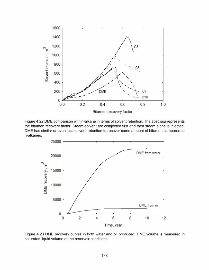
138

Figure 4.22 DME comparison with n-alkane in terms of solvent retention. The abscissa represents

the bitumen recovery factor. Steam-solvent are coinjected first and then steam alone is injected.

DME has similar or even less solvent retention to recover same amount of bitumen compared to

n-alkanes.

Figure 4.23 DME recovery curves in both water and oil produced. DME volume is measured in

saturated liquid volume at the reservoir conditions.

139

(1) 3-D reservoir

(2) Reservoir projection on the I-K plane

Figure 4.24 Reservoir dimensions for economic analysis. Producer is placed 2 m above the lower

reservoir boundary. Injector is 4 m above the producer. Well pair length is 500 m.

140

Figure 4.25 Net present value comparison. C10 has the maximum NPV, followed by DME, C7,

SAGD, C5 and C3.

Figure 4.26 Bitumen recovery for the first 5 years using different viscosity models. Case 1: DME

viscosity with C3 coefficients. Case 2: DME viscosity with C4 coefficients. Case 3: DME viscosity

with C5 coefficients. Case 4: C3 viscosity with C4 coefficients. Case 5: C5 viscosity with C4

coefficients.

141

Figure 4.27 Average drainage rate by using different viscosity models for DME. Case 1: DME

viscosity with C3 coefficients. Case 2: DME viscosity with C4 coefficients. Case 3: DME viscosity

with C5 coefficients. Case 4: C3 viscosity with C4 coefficients. Case 5: C5 viscosity with C4

coefficients.

142

Table 4.1 Critical properties and molecular weights for water/bitumen/DME ternary system.

Table 4.2 BIPs for water/bitumen/DME for the PR EOS. Ganjdanesh et al.’s (2015) BIPs are adjusted to better match experimental data.

Water CD DME

Water 0

CD 0.169 0

DME -0.170 0.075 0

Table 4.3 Water/DME VLLE experiment data from Pozo and Streett (1984).

T, K P, bar x_DME_W x_DME_L x_DME_V

323.15 10.27 0.155 0.814 0.958

348.15 18.00 0.128 0.781 0.936

373.26 28.48 0.104 0.755 0.910

394.21 40.54 0.090 0.727 0.901

400.49 44.40 0.089 0.725 0.879

403.26 46.61 0.087 0.721 0.862

414.00 54.54 0.081 0.705 0.844

423.5 62.19 0.093 0.736 0.832

427.4 66.05 0.104 0.755 -

Tc, K Pc, bar ω MW

Water 647.10 220.64 0.3433 18.01

CD 847.17 10.64 1.0406 530.00

DME 400.50 52.92 0.2000 46.07

143

Table 4.4 DME and n-C10 VLE experiment data from Park et al. (2007) at 323.15 K.

P, bar X_DME_L P, bar X_DME_L P, bar X_DME_L

0.0118 0 6.9302 0.6065 10.5442 0.9331

0.4214 0.0361 7.1749 0.6285 10.7261 0.9476

1.0284 0.0923 7.4478 0.6535 10.8867 0.9601

1.8317 0.1674 7.7211 0.6787 11.0195 0.9702

2.5537 0.2328 7.9177 0.6970 11.1274 0.9783

2.9252 0.2655 7.9959 0.7043 11.2147 0.9848

3.2081 0.2900 8.2660 0.7296 11.2749 0.9892

3.5784 0.3215 8.6044 0.7614 10.8867 0.9601

4.6748 0.4133 8.9313 0.7919 11.3175 0.9923

5.4953 0.4820 9.2424 0.8206 11.3452 0.9944

5.965 0.5219 9.5400 0.8476 11.3761 0.9966

6.3743 0.5573 9.8215 0.8725 11.4052 0.9987

6.6677 0.5831 10.0853 0.8952 11.4231 1

Table 4.5 DME and n-C12 VLE experiment data from Park et al. (2007) at 323.15 K.

P, bar X_DME_L P, bar X_DME_L P, bar X_DME_L

0.002 0 6.9709 0.6133 10.1592 0.8970

1.4515 0.1428 7.2175 0.6342 10.3951 0.9175

1.8914 0.1843 7.4722 0.6559 10.6101 0.9357

2.4681 0.2371 7.7524 0.6801 10.8083 0.9520

3.0536 0.2889 8.0324 0.7046 10.9675 0.9648

3.404 0.3191 8.3081 0.7290 11.1092 0.9758

3.7226 0.3461 8.5744 0.7530 11.2296 0.9850

4.2166 0.3873 8.7167 0.7659 11.3265 0.9922

5.1833 0.4666 9.0362 0.7950 11.3767 0.9959

5.9576 0.5296 9.3456 0.8234 11.4036 0.9978

6.3484 0.5616 9.6344 0.8498 11.4239 0.9993

6.6918 0.5900 9.906 0.8744 11.4339 1

Table 4.6 AARD between EOS prediction and experiment data with the calibrated EOS model.

Water/DME X_DME_W

Water/DME T three-phase

n-C10/DME X_DME_L

n-C12/DME X_DME_L

AARD, % 40.74 4.91 1.14 1.68

AAD 6.58 mol% 19.92 K 0.62 mol% 0.65 mol%

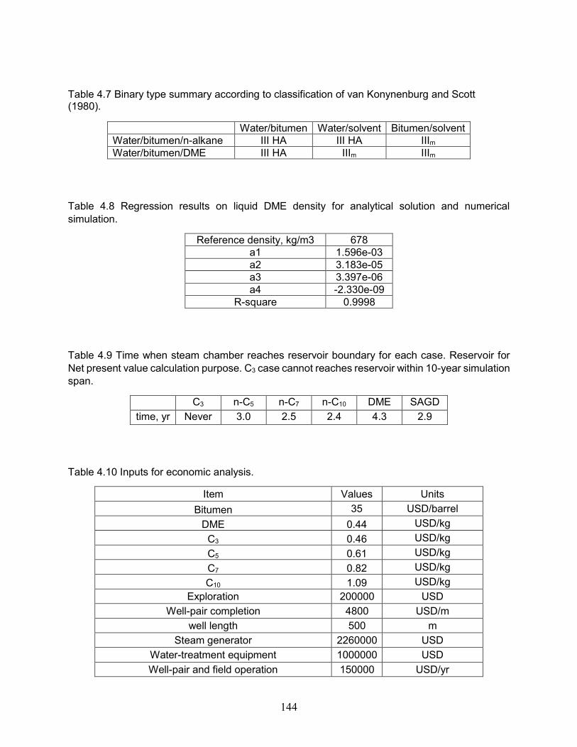
144

Table 4.7 Binary type summary according to classification of van Konynenburg and Scott (1980).

Water/bitumen Water/solvent Bitumen/solvent

Water/bitumen/n-alkane III HA III HA IIIm

Water/bitumen/DME III HA IIIm IIIm

Table 4.8 Regression results on liquid DME density for analytical solution and numerical

simulation.

Reference density, kg/m3 678

a1 1.596e-03

a2 3.183e-05

a3 3.397e-06

a4 -2.330e-09

R-square 0.9998

Table 4.9 Time when steam chamber reaches reservoir boundary for each case. Reservoir for

Net present value calculation purpose. C3 case cannot reaches reservoir within 10-year simulation

span.

C3 n-C5 n-C7 n-C10 DME SAGD

time, yr Never 3.0 2.5 2.4 4.3 2.9

Table 4.10 Inputs for economic analysis.

Item Values Units

Bitumen 35 USD/barrel

DME 0.44 USD/kg

C3 0.46 USD/kg

C5 0.61 USD/kg

C7 0.82 USD/kg

C10 1.09 USD/kg

Exploration 200000 USD

Well-pair completion 4800 USD/m

well length 500 m

Steam generator 2260000 USD

Water-treatment equipment 1000000 USD

Well-pair and field operation 150000 USD/yr

145

Administration and head office 7.48 USD/m3 oil

Blending and transportation 6.29 USD/m3 oil

Steam-generator operation 2.83 USD/m3 CWE

Fuel for steam generator 10.1 USD/m3 CWE

Treatment of water production 1.96 USD/m3 CWE

Solvent distribution line 100000 USD

Solvent handling 2000 USD/yr

Table 4.11 Maximum NPV and time achieved for each solvent coinjection. Solvent injection is

ceased immediately after steam chamber reaches the reservoir boundary.

C3 n-C5 n-C7 n-C10 DME SAGD

Max NPV, mil USD

-3.35 7.86 10.45 16.78 16.46 10.02

Time, yr 1.3 4.0 4.6 4.4 6.0 5.2

146

Chapter 5 Conclusions and Recommendations

This research has presented a systematic analysis on enhanced oil displacement efficiency

by steam-solvent coinjection based on thorough phase behavior study. This chapter summarizes

conclusions of previous chapters and gives suggestions for future works based on the

observations in this research.

5.1 Conclusions

In this research, a systematic phase behavior study for water/bitumen/solvent was given and

a classification method was proposed. The significance of this classification method is to

understand the ability of solvent mixing with bitumen on the steam chamber edge. The bitumen

mixing with solvent is the essential difference that makes coinjection different from SAGD. Then,

an algorithm was given to quantify the residual oil saturation for distillation based on the phase

behavior study. This algorithm used only thermodynamics to explain the residual oil saturation

due to the distillation, instead of solving mass balance or energy transfer equations as in

numerical simulation. The algorithm also provides a unified way to explain the differences in the

displacement efficiency by using different solvent or other conditions in coinjection. Finally, the

classification method and algorithm was applied to the coinjection of steam/DME, which is not

much studied so far.

Here are the key conclusions in this research:

Water/bitumen/solvent system can be classified into Ternary Types 1 and 2,

depending on whether solvent is completely miscible with bitumen without the

appearance of a second oleic phase L2. If solvent cannot completely mix with bitumen

and form L2, it is classified as Ternary Type 1. If within the operation temperature

range, only L1 exists, it is classified as Ternary Type 2.

147

Ternary Type 1 is unfavorable, because the solvent-rich L2 phase on the steam

chamber indicates poor solvent mixing with bitumen. Also, the L2 phase may extract

light components from the bitumen and impedes the flow of L1.

The distillation mechanisms can be explained in a unified way: the temperature

increase during distillation, and competition between solvent and water transfer from

the W and L phases to the V phase.

Lower residual oil saturation can be achieved if temperature increase is high, more

solvent and/or less water can be transferred from liquid to vapor during the distillation.

Lighter solvents, greater operation pressure and more solvent accumulation on the

chamber edge are favored in terms of displacement efficiency.

A preliminary research on the water/bitumen/DME system shows it is a Ternary Type

2 solvent at 35 bars. Because of the DME dissolution inside the water phase,

steam/DME coinjection may achieve higher chamber edge temperature than other

Ternary Type 1 n-alkanes. As a result, the drainage rate may be improved.

5.2 Recommendations

Throughout this research, accurately modeled phase behavior has been the key to explain

enhanced displacement efficiency by steam-solvent coinjection compared to SAGD. For non-

polar molecules as in the n-alkane models based upon latest experiment results, the PR EOS

and the vdW EOS were able to predict phase behavior accurately. However, the study regarding

DME in this research gives rather conservative results because of limitations of phase behavior

study using the PR EOS and the vdW mixing rules in dealing with mixtures containing DME. With

the current EOS model, the prediction of either three-phase temperature of water/DME or DME

dissolution in water is sacrificed however the BIP between water/DME is adjusted. Therefore, to

148

improve the understanding of ES-SAGD using DME, more advanced EOS model should be used

to accurately model both three-phase curve and solvent solubility in water.

Further, DME was classified as a Ternary Type 2 solvent at 35 bars in this research because

DME has limited ability to dissolve in bitumen at three-phase temperature of water/DME. However,

the phase behavior for bitumen/DME mixtures is still missing in the literature. PVT experiments

to determine the thermodynamics properties of DME-containing hydrocarbon systems should be

done in the future.

Also, the viscosity model in the simulations greatly impacts flows in the vicinity of chamber

edge and therefore impacts analysis involving drainage rate in this study. A lack of viscosity data

for DME-containing hydrocarbon mixtures created uncertainties in the discussion of DME

performance in coinjection. In the future, viscosity models for DME-containing mixtures can be

established by experiments to better understand the flow in steam-DME coinjection.

The whole research was focused on the phase behavior in steam-solvent coinjection. The

classification method was specifically developed to help explain the distillation and enhanced

displacement efficiency. However, it is possible to develop a more general classification method

for ternary system that is not limited to the practice of steam-solvent coinjection, for the pure

interest of theoretical study.

149

References

Amani, M.J., Gray, M.R. and Shaw, J.M., 2013. Phase behavior of Athabasca bitumen+ water

mixtures at high temperature and pressure. The Journal of Supercritical Fluids, 77, pp.142-

152.

Amani, M.J., Gray, M.R. and Shaw, J.M., 2013. Volume of mixing and solubility of water in

Athabasca bitumen at high temperature and pressure.Fluid Phase Equilibria, 358, pp.203-211.

Blevins, T.R., Aseltine, R.J. and Kirk, R.S., 1969. Analysis of a steam drive project, Inglewood

Field, California. Journal of Petroleum Technology, 21(09), pp.1-141.

Blevins, T.R. and Billingsley, R.H., 1975. The Ten-Pattern Steamflood, Kern River Field,

California. Journal of Petroleum Technology, 27(12), pp.1-505.

Boshkov, L.Z., 1987. On the description of closed-loop phase-diagrams of 2-component solutions,

based on the one-fluid equation of state. DOKLADY AKADEMII NAUK SSSR, 294(4), pp.901-

905.

Brunner, E., 1988. Fluid mixtures at high pressures VI. Phase separation and critical phenomena

in 18 (n-alkane+ ammonia) and 4 (n-alkane+ methanol) mixtures. The Journal of Chemical

Thermodynamics, 20(3), pp.273-297.

Brunner, E., 1990. Fluid mixtures at high pressures IX. Phase separation and critical phenomena

in 23 (n-alkane+ water) mixtures. The Journal of Chemical Thermodynamics, 22(4), pp.335-

353.

Brunner, E., Thies, M.C. and Schneider, G.M., 2006. Fluid mixtures at high pressures: Phase

behavior and critical phenomena for binary mixtures of water with aromatic hydrocarbons. The

Journal of supercritical fluids, 39(2), pp.160-173.

Butler, R.M., 1997. Thermal recovery of oil and bitumen, publ. GravDrain Inc.(2nd printing),

Calgary, Alberta, 528pp.

150

Chernetsky, A., Masalmeh, S., Eikmans, D., Boerrigter, P.M., Fadili, A., Parsons, C.A., Parker,

A., Boersma, D.M., Cui, J., Dindoruk, B. and te Riele, P.M., 2015, November. A Novel

Enhanced Oil Recovery Technique: Experimental Results and Modelling Workflow of the DME

Enhanced Waterflood Technology. In Abu Dhabi International Petroleum Exhibition and

Conference. Society of Petroleum Engineers.

Computer Modelling Group, 2013. STARS version 2013 user's guide. Computer Modelling Group,

Calgary, Alberta, Canada.

Computer Modelling Group, 2013. WINPROP version 2013 user's guide. Computer Modelling

Group, Calgary, Alberta, Canada.

Connolly, J.F., 1966. Solubility of Hydrocarbons in Water Near the Critical Solution

Temperatures. Journal of Chemical and Engineering data, 11(1), pp.13-16.

Constantinou, L. and Gani, R., 1994. New group contribution method for estimating properties of

pure compounds. AIChE Journal, 40(10), pp.1697-1710.

Constantinou, L., Gani, R. and O'Connell, J.P., 1995. Estimation of the acentric factor and the

liquid molar volume at 298 K using a new group contribution method. Fluid Phase

Equilibria, 103(1), pp.11-22.

Deiters, U.K. and Kraska, T., 2012. High-Pressure Fluid Phase Equilibria: Phenomenology and

Computation (Vol. 2). Elsevier.

Dong, L., 2012. Effect of vapour–liquid phase behaviour of steam–light hydrocarbon systems on

steam assisted gravity drainage process for bitumen recovery. Fuel, 95, pp.159-168.

Ganjdanesh, R., Rezaveisi, M., Pope, G.A. and Sepehrnoori, K., 2015, September. Treatment of

Condensate and Water Blocks in Hydraulic Fractured Shale Gas-Condensate Reservoirs.

In SPE Annual Technical Conference and Exhibition. Society of Petroleum Engineers.

Gao, J., Okuno, R. and Li, H.A., 2016, June. An Experimental Study of Multiphase Behavior for

n-Butane/Bitumen/Water Mixtures. In SPE Canada Heavy Oil Technical Conference. Society

of Petroleum Engineers.

151

Gates, I.D., 2007. Oil phase viscosity behaviour in expanding-solvent steam-assisted gravity

drainage. Journal of Petroleum Science and Engineering,59(1), pp.123-134.

Govind, P.A., Das, S.K., Srinivasan, S. and Wheeler, T.J., 2008, January. Expanding solvent

SAGD in heavy oil reservoirs. In International Thermal Operations and Heavy Oil Symposium.

Society of Petroleum Engineers.

Gupta, S.C. and Gittins, S.D., 2006. Christina Lake Solvent Aided Process Pilot. Journal of

Canadian Petroleum Technology, 45(09).

Ignasiak, B.L., Yamaoka, K., 2010. In-situ recovery of bitumen or heavy oil by injection of di-

methyl ether. https://www.google.ca/patents/CA2652930A1?cl=en. Google Patents.

Ihmels, E.C. and Lemmon, E.W., 2007. Experimental densities, vapor pressures, and critical point,

and a fundamental equation of state for dimethyl ether. Fluid Phase Equilibria, 260(1), pp.36-

48.

Jha, R.K., Kumar, M., Benson, I. and Hanzlik, E., 2013. New insights into steam/solvent-

coinjection-process mechanism. SPE Journal, 18(05), pp.867-877.

Keshavarz, M. and Chen, Z., 2014, October. Modeling Displacement Efficiency Improvement

During Solvent Aided-SAGD. In SPE Annual Technical Conference and Exhibition. Society of

Petroleum Engineers.

Keshavarz, M., Okuno, R. and Babadagli, T., 2014. Efficient oil displacement near the chamber

edge in ES-SAGD. Journal of Petroleum Science and Engineering, 118, pp.99-113.

Keshavarz, M., Okuno, R. and Babadagli, T., 2015 (a). A semi-analytical solution to optimize

single-component solvent coinjection with steam during SAGD. Fuel, 144, pp.400-414.

Keshavarz, M., Okuno, R. and Babadagli, T., 2015 (b). Optimal Application Conditions for

Steam/Solvent Coinjection. SPE Reservoir Evaluation & Engineering, 18(01), pp.20-38.

Kumar, A., 2016. Characterization of Reservoir Fluids based on Perturbation from n-Alkanes.

ERA thesis of University of Alberta.

152

Kumar, A. and Okuno, R., 2015, September. A New Algorithm for Multiphase Fluid

Characterization for Solvent Injection. In SPE Annual Technical Conference and Exhibition.


Kumar, A. and Okuno, R., 2016. Reliable characterization of bitumen based on perturbation from

n-alkanes for steam-solvent coinjection simulation.Fuel, 182, pp.141-153.

Leaute, R.P., 2002, January. Liquid addition to steam for enhancing recovery (LASER) of bitumen

with CSS: Evolution of technology from research concept to a field pilot at Cold Lake. In SPE

International Thermal Operations and Heavy Oil Symposium and International Horizontal Well

Technology Conference. Society of Petroleum Engineers.

Leaute, R.P. and Carey, B.S., 2007. Liquid addition to steam for enhancing recovery (LASER) of

bitumen with CSS: Results from the first pilot cycle.Journal of Canadian Petroleum

Technology, 46(09).

Li, W., Mamora, D.D. and Li, Y., 2011a. Solvent-type and-ratio impacts on solvent-aided SAGD

process. SPE Reservoir Evaluation & Engineering,14(03), pp.320-331.

Li, W., Mamora, D. and Li, Y., 2011b. Light-and heavy-solvent impacts on solvent-aided-SAGD

process: a low-pressure experimental study. Journal of Canadian Petroleum

Technology, 50(04), pp.19-30.

Nasr, T.N. and Ayodele, O.R., 2006, January. New hybrid steam-solvent processes for the

recovery of heavy oil and bitumen. In Abu Dhabi International Petroleum Exhibition and


Nasr, T.N., Beaulieu, G., Golbeck, H. and Heck, G., 2003. Novel Expanding Solvent-SAGD

Process" ES-SAGD". Journal of Canadian Petroleum Technology, 42(01).

Nghiem, L.X. and Li, Y.K., 1984. Computation of multiphase equilibrium phenomena with an

equation of state. Fluid Phase Equilibria, 17(1), pp.77-95.

153

Ohno, Y., Inoue, N., Okuyama, K. and Yajima, T., 2005, January. New clean fuel DME.

In International Petroleum Technology Conference. International Petroleum Technology

Conference.

Okuno, R., Johns, R. and Sepehrnoori, K., 2010. A new algorithm for Rachford-Rice for

multiphase compositional simulation. SPE Journal, 15(02), pp.313-325.

Orr, B., 2009, January. ES-SAGD; Past, Present and Future. In SPE Annual Technical

Conference and Exhibition. Society of Petroleum Engineers.

Park, S.J., Han, K.J. and Gmehling, J., 2007. Isothermal phase equilibria and excess molar

enthalpies for binary systems with dimethyl ether at 323.15 K. Journal of Chemical &

Engineering Data, 52(5), pp.1814-1818.

Park, K.J., Seo, T. and Jung, D., 2007. Performance of alternative refrigerants for residential air-

conditioning applications. Applied energy,84(10), pp.985-991.

Pozo, M.E. and Streett, W.B., 1984. Fluid phase equilibria for the system dimethyl ether/water

from 50 to 220. degree. C and pressures to 50.9 MPa.Journal of Chemical and Engineering

Data, 29(3), pp.324-329.

Prats, M., 1982. Thermal recovery.

Qian, J.W., Privat, R. and Jaubert, J.N., 2013. Predicting the Phase Equilibria, Critical

Phenomena, and Mixing Enthalpies of Binary Aqueous Systems Containing Alkanes,

Cycloalkanes, Aromatics, Alkenes, and Gases (N2, CO2, H2S, H2) with the PPR78 Equation

of State. Industrial & Engineering Chemistry Research, 52(46), pp.16457-16490.

Rebert, C.J. and Kay, W.B., 1959. The phase behavior and solubility relations of the benzene‐

water system. AIChE Journal, 5(3), pp.285-289.

Riazi, M.R. and Daubert, T.E., 1987. Characterization parameters for petroleum

fractions. Industrial & engineering chemistry research, 26(4), pp.755-759.

154

Schneider, G.M., 2002. Aqueous solutions at pressures up to 2 GPa: gas–gas equilibria, closed

loops, high-pressure immiscibility, salt effects and related phenomena. Physical Chemistry

Chemical Physics, 4(6), pp.845-852.

Scott, R.L. and van Konynenburg, P.H., 1970. Static properties of solutions. Van der Waals and

related models for hydrocarbon mixtures. Discussions of the Faraday society, 49, pp.87-97.

Tallon, S. and Fenton, K., 2010. The solubility of water in mixtures of dimethyl ether and carbon

dioxide. Fluid Phase Equilibria, 298(1), pp.60-66.

van Konynenburg, P.H. and Scott, R.L. 1980. Critical lines and phase equilibria in binary van der

Waals mixtures. Philosophical Transactions of the Royal Society of London A: Mathematical,

Physical and Engineering Sciences 298(1442): 495-540.

Venkatramani, A.V. and Okuno, R., 2014, June. Modeling of Multiphase Behavior for Water/n-

Alkane Mixtures by Use of the Peng-Robinson EOS. In SPE Heavy Oil Conference-Canada.


Venkatramani, A.V. and Okuno, R., 2015. Characterization of water-containing reservoir oil using

an EOS for steam injection processes. Journal of Natural Gas Science and Engineering, 26,

pp.1091-1106.

Venkatramani, A.V. and Okuno, R., 2016, June. Compositional Mechanisms in SAGD and ES-

SAGD With Consideration of Water Solubility in Oil. In SPE Canada Heavy Oil Technical


Volek, C.W. and Pryor, J.A., 1972. Steam distillation drive-Brea field, California. Journal of

Petroleum Technology, 24(08), pp.899-906.

Willman, B.T., Valleroy, V.V., Runberg, G.W., Cornelius, A.J. and Powers, L.W., 1961. Laboratory

studies of oil recovery by steam injection. Journal of Petroleum Technology, 13(07), pp.681-

690.

Wong, D.S.H. and Sandler, S.I., 1992. A theoretically correct mixing rule for cubic equations of

state. AIChE Journal, 38(5), pp.671-680.

155

Wu, J., Liu, Z., Bi, S. and Meng, X., 2003. Viscosity of saturated liquid dimethyl ether from (227

to 343) K. Journal of Chemical & Engineering Data,48(2), pp.426-429.

156

Appendices

Appendix A. Peng-Robinson Equation of State and van der Waals Mixing Rules

Peng and Robinson (1978) suggested cubic EOS for pure component in the following form,

𝑃 =𝑅𝑇

𝑉 − 𝑏−

𝑎(𝑇)

𝑉(𝑉 + 𝑏) + 𝑏(𝑉 − 𝑏)

(A.1)

where,

𝑎(𝑇) = 0.45724 𝑅2𝑇𝑐

2

𝑃𝑐𝛼(𝑇) (A.2)

𝛼(𝑇) = (1 + 𝑚 (1 − √𝑇

𝑇𝑐))

2

(A.3)

𝑚 = 0.37464 + 1.54226𝜔 − 0.26992𝜔2 (𝜔 < 0.49) (A.4a)

𝑚 = 0.379642 + 1.48503𝜔 − 0.164423𝜔2 + 0.016666𝜔3 (𝜔 > 0.49) (A.4b)

𝑏 =0.07780𝑅𝑇𝑐

𝑃𝑐 (A.5)

For mixtures, pure component a and b should be mixed according to certain rules, such as

the vdW mixing rules shown as follows,

𝑎 = ∑ ∑ 𝑥𝑖𝑥𝑗√𝑎𝑖𝑎𝑗𝑁𝑐1

𝑁𝑐1 (1-BIP) (A.6)

𝑏 = ∑ 𝑥𝑖𝑏𝑖

𝑁𝑐

1 (A.7)

157

Appendix B. Liquid Density Correlations of the CMG STARS (2013)

In the CMG STARS (2013), liquid phase density such as aqueous and oleic phase is

calculated by linear mixing of pure component density,

𝜌𝑗 = ∑ 𝑥𝑖𝑗𝜌ij𝑁𝑐𝑖=1 , (B.1)

where,

𝜌𝑗, molar density of liquid phase j,

𝑥𝑖𝑗, mole fraction of component i in liquid phase j,

𝜌𝑖𝑗, density of component i in phase j at T and P, which can be calculated in the following way.

𝜌ij = 𝜌𝑖𝑟𝑒𝑓 exp[−𝛼1(𝑇 − 𝑇𝑟𝑒𝑓) −1

2𝛼2(𝑇2 − 𝑇𝑟𝑒𝑓

2)

+𝛼3(𝑃 − 𝑃𝑟𝑒𝑓) + 𝛼4(𝑃 − 𝑃𝑟𝑒𝑓)(𝑇 − 𝑇𝑟𝑒𝑓)]

(B.2)

where,

𝑃𝑟𝑒𝑓, the reference pressure, 1.01325 bars.

𝑇𝑟𝑒𝑓, the reference temperature, 288.15 K.

𝜌𝑖𝑟𝑒𝑓, pure component i molar density at reference pressure and temperature.

α1, the first coefficient of the thermal expansion correlation of component i, 1

𝐾.

α2, the second coefficient of the thermal expansion correlation of component i, 1

𝐾2.

α3, liquid compressibility at constant temperature of component i, 100

𝑏𝑎𝑟.

α4, pressure-temperature cross term for liquid density of component i, 100

𝑏𝑎𝑟.𝐾.

Documents

Master of Science in Petroleum Engineering Department of ... · analytical solution developed in this research is a first thermodynamics tool to estimate the displacement efficiency