Embed Size (px)
DESCRIPTION
Mass Balancing Example
Citation preview

HSC Chemistry® 7.0 49 - 1
Pertti Lamberg October 15, 2009 09006-ORC-J
49. MASS BALANCING AND DATA RECONCILIATION
EXAMPLES
This manual gives examples how to solve different kind of mass balancing problems. Please
have a look of the manual “48. Sim Mass Balancing” for detailed information of different
buttons and menus.
49. MASS BALANCING AND DATA RECONCILIATION EXAMPLES .................................................... 1
49.1. MASS BALANCING AND DATA RECONCILIATION ....................................................................................... 1 49.2. EXAMPLE 1 - 1D COMPONENTS ................................................................................................................. 2 49.3. EXAMPLE 2 – 1D CHEMICAL COMPONENTS ............................................................................................. 20 49.4. EXAMPLE 3 – 1D MINERALS .................................................................................................................... 24 49.5. EXAMPLE 4 – 1.5D MASS BALANCING .................................................................................................... 36 49.6. EXAMPLE 5 – 2D CHEMICAL COMPONENTS ............................................................................................. 41 49.7. EXAMPLE 6 – MULTIPLE DATA SETS ....................................................................................................... 46
49.1. Mass Balancing and Data Reconciliation
Mass balancing is a common practice in metallurgy. The mass balance of a circuit is needed
for several reasons: 1) To estimate the metallurgical performance of the circuit. 2) To locate
process bottlenecks and for circuit diagnosis. 3) To create models of the processing stages. 4)
To simulate the process.
The following steps are often required to simulate a process:
1. Collecting experimental data (experimental work, sampling, sample
preparation, assaying)
2. Mass balancing and data reconciliation of the experimental data
3. Model building
4. Simulation
HSC7 allows the user to solve the following mass balance problems (Table 1):
1. Reconcile measured or estimated component flowrates (1D components).
2. Mass balance and reconcile chemical analyses (1D assays)
3. Mass balance minerals in minerals processing circuit (1D Minerals)
4. Mass balance size distribution and water balance (1.5D)
5. Mass balance assays and components in 2- or 3-phase systems where the bulk composition
is not analyzed (2D Components)
6. Mass balance minerals or chemical assays size-by-size (2D Assays)
7. Mass balance particles, MLA assays (3D)
This manual includes mass balance and data reconciliation examples of following problems:
1. 1D Components (chapter 49.2)
2. 1D assays (chapter 49.3)
3. 1D minerals (chapter 49.4)
4. 1.5D (chapter 49.5)
5. 2D analyses (chapter 49.6)
6. Multiple data sets (chapter 49.7)

HSC Chemistry® 7.0 49 - 2
Pertti Lamberg October 15, 2009 09006-ORC-J
Table 1. Mass balance cases that can be solved with HSC Sim. The red X indicates that data is
necessary and defines the case. In order to solve the 3D-mass balance, the particle tracking
module of HSC is required. This is currently available only for AMIRA P9O Sponsors.
Assayed or | Case estimated values |
1D Components
1D Assays
1D Minerals
1.5D 2D Assays
2D Minerals
3D
Total stream flowrates X
Total solid flowrates X X X X X X X
Liquid flowrates X (X) (X) (X)
Component flowrates X
Component distributions X
%Solids (X) (X) (X) (X) (X) (X)
Bulk chemical compositions X X X X X
Minerals and their chemical composition
X X X
Particle size distribution X X X X
Chemical composition of size fractions
X X X
Particles (MLA data) X
49.2. Example 1 - 1D Components
The 1D components balancing exercise can be found in
C:\HSC7\Flowsheet_MassBalancing\Example 1D Components. To jump over the drawing
and bringing the experimental data just open the “1D Component Example.fls” file.
In this exercise we have a circuit with five units and eleven streams. We want to get the
balance for arsenic and copper flowrates through the circuit. We have measured the flowrate
information only from the input and output streams. In addition we have the knowledge on
the distribution of the component between the output streams of each of the unit. This data
could be metallurgical knowledge of specific process stages.
Figure 1. Example 1D can be found in your computer.
49.2.1. Draw the flowsheet
Open HSC Sim.

HSC Chemistry® 7.0 49 - 3
Pertti Lamberg October 15, 2009 09006-ORC-J
1. Turn the HSC mode to Experimental (Figure 2) 2. Draw first the units; the example has five units named as U1, U2, U3, U4
and U5 (Figure 3) 3. Draw the streams; the example has eleven streams called as letters form A
to J. Be sure that the Source and Destinations are correct (Figure 3) 4. Finally check the stream connections using the “Overlay and Route Check”
button as shown below. The input streams are shown blue, the output streams red and the intermediate streams black .
5. Save the drawing.
Figure 2. Turning the mode to Experimental.
Figure 3. Flowsheet of Example 1.

HSC Chemistry® 7.0 49 - 4
Pertti Lamberg October 15, 2009 09006-ORC-J
49.2.2. Bring in the experimental data The experimental data is collected in the Analyses.xls file which is to be stored in the very same folder you saved the flowsheet drawing file. To import the data using Excel:
1. Open the Analyses.xls file in MS Excel. 2. In HSC go to the Analyses window (Experimental – Analyses, Figure 4).
Create Stream Properties sheet: Select from the menu “Create – Stream Properties Sheet – Horizontal” (Figure 6)
3. In the MS Excel copy the experimental data into the clipboard. The cell “Stream” must be the first cell on top left (Figure 6).
4. In HSC Sim go to the Experimental data and select Edit – Paste Special – Assays” (Figure 7).
5. To visualize the data in the flowsheet create the value labels: press Visualize and select “Create Stream Value Labels” (Figure 8).
6. In the Analyses window select column to visualize the variable in the flowsheet (Figure 9).
Figure 4. Experimental data.
Figure 5. Creating Stream Properties Sheet.

HSC Chemistry® 7.0 49 - 5
Pertti Lamberg October 15, 2009 09006-ORC-J
Figure 6. Copying data into clipboard. The first cell on left top corner has to be the “Stream” cell.
Figure 7. Pasting assays.

HSC Chemistry® 7.0 49 - 6
Pertti Lamberg October 15, 2009 09006-ORC-J
Figure 8. Creating Stream Value Labels.

HSC Chemistry® 7.0 49 - 7
Pertti Lamberg October 15, 2009 09006-ORC-J
Figure 9. Visualizing variable in the flowsheet.
49.2.3. Mass Balancing Wizard
To mass balance the data:
1. Press “Mass Balancing and Data Reconciliation>>>” in the Analyses –window (Figure 10).
2. Check that As and Cu flowrates are identified correctly as “CD – Component Flowrates” and As and Cu distributions as “CD – Component Distribution” (Figure 11). Press Next.
3. In the second wizard window (step 2 of 5) check that all streams are selected for the mass balancing (Figure 12). Press Next.
4. In the Step 3 you can edit the error models. Here we use the default values, i.e. flowrates the relative error is 10%, detection limit is 0.1 and max standard deviation is 10 tph. For distribution the relative error is 10%, detection limit 1% and max standard deviation is 10 percentage values. (Figure 13). Press Next.
5. Step 4; the reference stream is “A”. Press Next (Figure 14). 6. Step 5. Errors and mass balance nodes. There should not be any errors.
Press Next (Figure 15).

HSC Chemistry® 7.0 49 - 8
Pertti Lamberg October 15, 2009 09006-ORC-J
Figure 10. Press ”Balance and Data Reconciliation >>>” button.
Figure 11. The Mass Balance wizard, step 1.

HSC Chemistry® 7.0 49 - 9
Pertti Lamberg October 15, 2009 09006-ORC-J
Figure 12. Step 2.

HSC Chemistry® 7.0 49 - 10
Pertti Lamberg October 15, 2009 09006-ORC-J
Figure 13. Step 3.

HSC Chemistry® 7.0 49 - 11
Pertti Lamberg October 15, 2009 09006-ORC-J
Figure 14. Step 4. Reference stream
Figure 15. Step 5. Nodes, node 4 is visualized: blue streams are the feed streams of the node, red
ones are the output streams. Narrow black streams are not included in the node 4. Number oif
errors is zero.

HSC Chemistry® 7.0 49 - 12
Pertti Lamberg October 15, 2009 09006-ORC-J
49.2.4. Mass Balancing Window After the mass balancing wizard you can see the Data Balancing and Reconciliation window
(Figure 16). The left part of the window shows Dimension selector and Step Navigator
(Figure 17) and Data indicator (Figure 18). In the middle you can see the Data Sheet (Figure
19). On right hand side you can see the Balance/Report Options. To solve the mass
balancing problem press or button.
Figure 16. Mass Balancing and Data Reconciliation window.
Figure 17. Navigator including dimension selector and step navigator.

HSC Chemistry® 7.0 49 - 13
Pertti Lamberg October 15, 2009 09006-ORC-J
Figure 18. Data indicator.
Figure 19. Data sheet.

HSC Chemistry® 7.0 49 - 14
Pertti Lamberg October 15, 2009 09006-ORC-J
Figure 20. Balance/Report options.
Once you press the press or button HSC Sim
solves the mass balance problem. Balanced (Bal) columns become visible, i.e. now you have
visible measured values (white background) and balanced values (grey background). To see
more columns check the ones you want to see in the report options / column selector (Figure
22). To visualize the balance in the flowsheet click the column in the data sheet (Figure 23)
and see the flowsheet (Figure 24). Use copy/paste to report out for example in MS Word.
Now HSC Sim has adjusted all arsenic tonnages, but we would like to see the feed tonnages,
100 tph, remain unchanged. There are two options for that: 1) set the standard deviation for
the stream A / As tph very small, say 0.01 (Figure 25); 2) set the minimum and maximum
values to 100 and 100 and select the solution method to CLS (Constrained Least Squares)
(Figure 26).
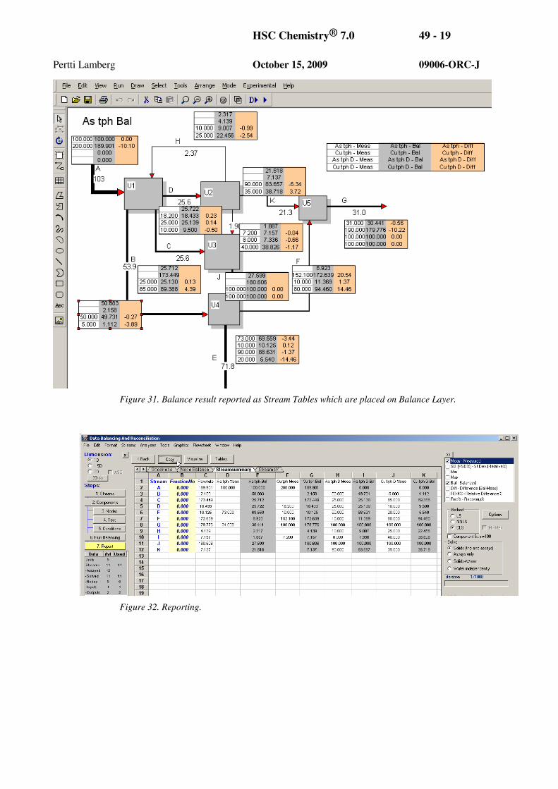
To report result as Stream Tables, Select from the menu “Flowsheet – Create Stream Tables”
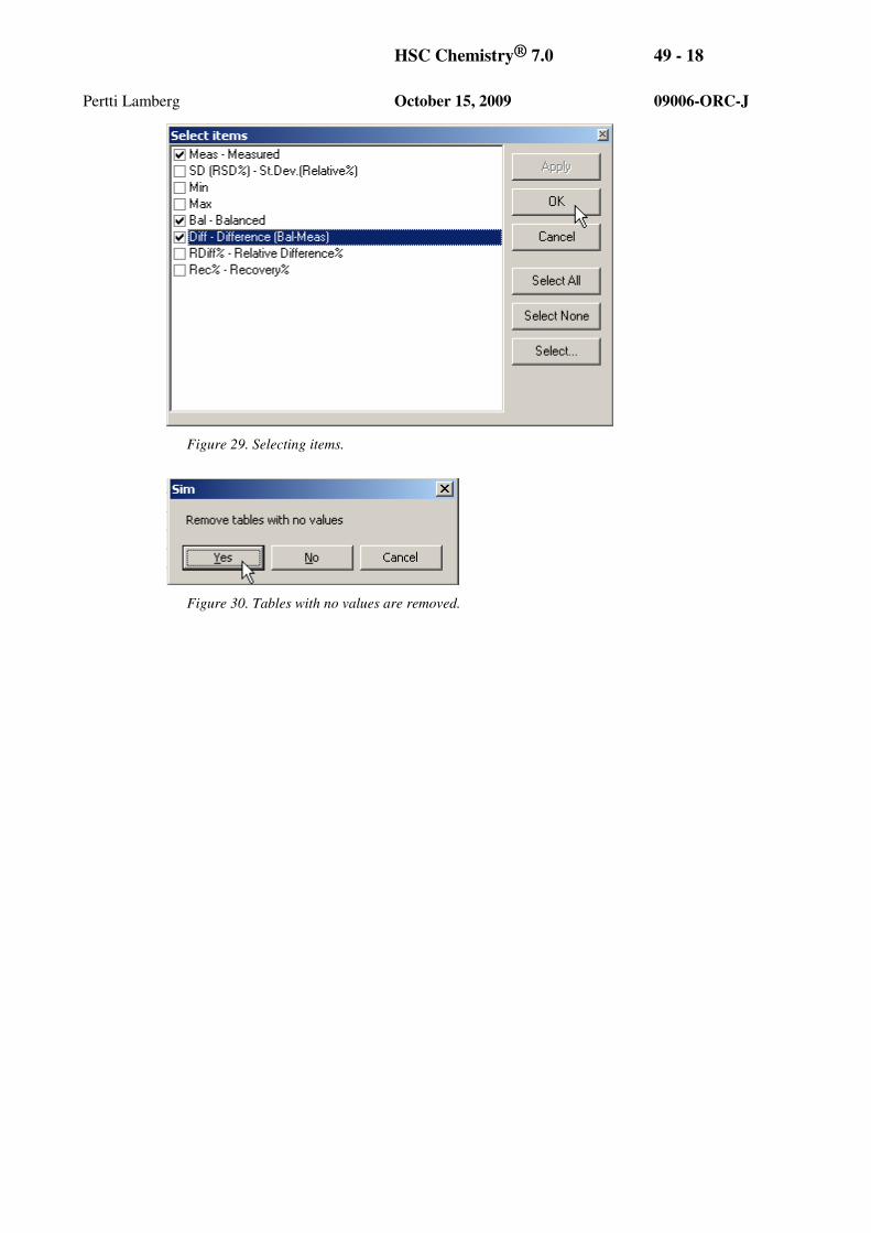
(Figure 27), select the components (Figure 28) and items (Figure 29). In the next window
answer “Yes” to remove the tables with no values (Figure 30). Oranize the tables in the
flowsheet in a way that all tables and streams can be seen (Figure 31). Use copy/paste to
report out.
Click Report and in the StreamSummary sheet select reported items and press Copy to get
the data into the clipboard (Figure 32). Paste into for example MS Excel.

HSC Chemistry® 7.0 49 - 15
Pertti Lamberg October 15, 2009 09006-ORC-J
To save the full result select File – Save and give a name for the file (Figure 33).
Figure 21. Mass Balance solved and data reconciled.
Figure 22. Report options; column selector.
Figure 23. Clicking As tph to visualize in the flowsheet (see next figure).

HSC Chemistry® 7.0 49 - 16
Pertti Lamberg October 15, 2009 09006-ORC-J
Figure 24. Selected item reported in the flowsheet.
Figure 25. As tph for the stream A set to 0.001. Now balanced As tph is practically equal to the
measured one.

HSC Chemistry® 7.0 49 - 17
Pertti Lamberg October 15, 2009 09006-ORC-J
Figure 26. Setting min and max values for As to 100 and 100 and pressing Balance will solve the
As flowrate using constraints. Remember to change the solution method to CLS (Constrained
Least Squares).
Figure 27. Create Stream Tables.
Figure 28. Selecting components to be reported.
HSC Chemistry® 7.0 49 - 18
Pertti Lamberg October 15, 2009 09006-ORC-J
Figure 29. Selecting items.
Figure 30. Tables with no values are removed.
HSC Chemistry® 7.0 49 - 19
Pertti Lamberg October 15, 2009 09006-ORC-J
Figure 31. Balance result reported as Stream Tables which are placed on Balance Layer.
Figure 32. Reporting.

HSC Chemistry® 7.0 49 - 20
Pertti Lamberg October 15, 2009 09006-ORC-J
Figure 33. Saving balance file.
49.3. Example 2 – 1D Chemical Components
The 1D Chemical Components example can be found in
C:\HSC7\Flowsheet_MassBalancing\Example Copper Circuit. The file is Copper Circuit.fls
(Figure 33). In the Experimental Data select sheet “5 1D with ERROR” (Figure 34).
In the Mass Balance Wizards keep the default values, or you can even Skip the wizards
(Figure 35). In the Data Balancing and Reconciliation press or
button to solve the mass balance.
With the basic options you will find that there are some negative numbers and %Solids and
Water have not been solved (Figure 36). To overcome the negative values select Non-
Negative Least Squares (NNLS) method. For solving also water and %solids select
Solids+water of Water Independently. The former solves all simultaneously the latter solves
first solids and then solves %solids and Water using Solids solution as constraints.
Now mass balance result does not have any negative values and Water and %Solids are also
solved. However, the Mill Water has 0.65 t/h solids and ROM has been adjusted to 114 t/h.
For the former we set min and max to zero and latter min=max=112 t/h (Figure 39). The
solutions is showed in Figure 40.

HSC Chemistry® 7.0 49 - 21
Pertti Lamberg October 15, 2009 09006-ORC-J
Figure 34. Select sheet ”5 1D with ERROR”.
Figure 35. Press Skip Wizard, the default values will be used.

HSC Chemistry® 7.0 49 - 22
Pertti Lamberg October 15, 2009 09006-ORC-J
Figure 36. Negative results and %Solids Balanced values are zeros.
Figure 37. NNLS and Water Independently selected.

HSC Chemistry® 7.0 49 - 23
Pertti Lamberg October 15, 2009 09006-ORC-J
Figure 38. Total Solids flowrate, balanced. Mill Water has 0.65 t/h solids which is not right.
Figure 39. Constraints for totals solids t/h.

HSC Chemistry® 7.0 49 - 24
Pertti Lamberg October 15, 2009 09006-ORC-J
Figure 40. Mass balance of the 1D case.
49.4. Example 3 – 1D Minerals
In 1D minerals we use the vary same example as above, i.e.
C:\HSC7\Flowsheet_MassBalancing\Example Copper Circuit. The file is Copper Circuit.fls
(Figure 33) and the sheet “5 1D with ERROR” (Figure 34).
When mass balancing with minerals the steps are:
1. Convert elemental grades to mineral grades using HSCGeo
2. Bring the mineral matrix into HSC Sim
3. Solve mineral balance using constraint Sum=100.
4. Bring the solution back to Analyses.
5. Calculate Minerals to Element.
To convert elemental grades to mineral grades select the correct sheet and select Tools –
Element To Mineral Conversions – Using HscGeo (Figure 41). In HscGeo press Define >>>
to define minerals (Figure 42). Type “chalcopyrite” and select the stoichiometric one and
press Add (Figure 43). Continue by adding pyrite and quartz (Figure 44) and press OK to
return to Modal Calculation window. Now select Ccp (chalcopyrite) and press > -button to
move it to calculation list (Figure 45). Press “Cu” to define that chalcopyrite is calculated
from copper (Figure 46). We are confident of copper assays and that chalcopyrite is the only
copper mineral and its’ composition is stoichiometric. For pyrite we are not so sure.
Therefore we will calculate pyrite on the second round using both S and Fe (Figure 47).

HSC Chemistry® 7.0 49 - 25
Pertti Lamberg October 15, 2009 09006-ORC-J
The remaining, quartz, is calculated from 100-others, use right mouse button for selecting
that option (Figure 48). Press Run to calculate the modal composition (Figure 49). In two
samples the mineral sum is higher than 100% (Figure 50). This is due to uncertainties in S
and Fe assays which means that our estimate on pyrite is too high. To fix that we use
“Normalize” button (Figure 51) define that pyrite is adjusted by selecting ”Py”, ”Total sum
is” and ”100” and press Calculate (Figure 52). Now the modal calculation is ready. Select
from the menu Edit – Copy the Whole Sheet (With Headers) (Figure 53).
Now move back to HSC Sim, activate the “Experimental Data” and select Edit – Paste
Special Assays (Figure 54). Mineral analyses are now pasted to HSC Sim (Figure 55). To
have the possibility for calculating back to elements go once again back to HscGeo and
select Edit – Copy Mineral Matrix (Figure 56), move back to HSC Sim and select Tools –
Paste Mineral Matrix (Figure 57). HSC Sim crates a sheet named MinrealMatrix and brings
the chemical composition of minerals on that sheet (Figure 58).
Now get back to the sheet “5 1D with ERROR” and press
-button. In the first Balance Wizard step select
“Total Solids Flowrate”, “%Solids”, “Water”, “Ccp”, “Py”, and “Qtz” (Figure 59). You can
skip the other steps (press Skip Wizard).
In the Data Balancing and Reconciliation window set the method to “CLS”, check the
“Component Sum=100”, Solve “Water Independently”, set the min and max values for water
streams to zero and for ROM to 112. Press solve; the result is shown in Figure 61. For
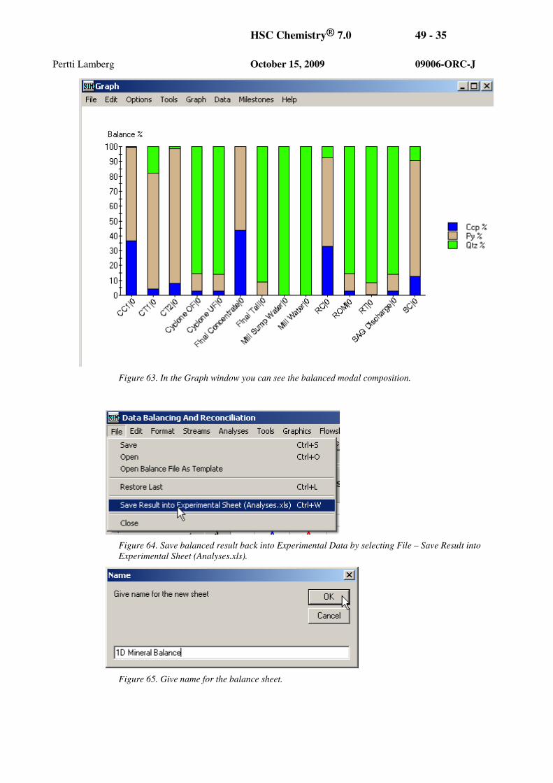
graphical presentation select Graphics – Assays Stacked Bar (Figure 62, Figure 63).
To calculate back to elements result has to be moved back to Experimental Data; use “File –
Save Result into Experimental Sheet (Analyses.xls)” (Figure 64). Give name for the balance
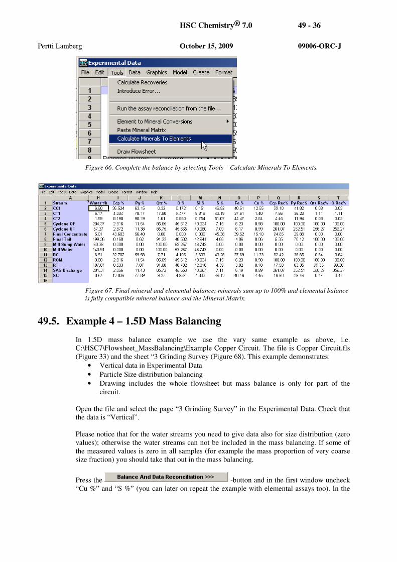
sheet (Figure 65) and complete the balance by selecting “Tools – Calculate Minerals To
Elements” (Figure 66). Now the balance is ready. In the final mineral and elemental balance
minerals sum up to 100% and elemental balance is fully compatible mineral balance and the
Mineral Matrix (Figure 67).
Figure 41. Element to Mineral Conversions, starting HscGeo.

HSC Chemistry® 7.0 49 - 26
Pertti Lamberg October 15, 2009 09006-ORC-J
Figure 42. In HscGeo press Define >>> to define minerals.
Figure 43. Adding chalcopyrite.

HSC Chemistry® 7.0 49 - 27
Pertti Lamberg October 15, 2009 09006-ORC-J
Figure 44. Chalcopyrite, pyrite and quartz added.
Figure 45. Moving Ccp (chalcopyrite) to calculation list.
Figure 46. Chalcopyrite –Cu selected for the first round, pressing UP-button to move to the
second round.

HSC Chemistry® 7.0 49 - 28
Pertti Lamberg October 15, 2009 09006-ORC-J
Figure 47. Second round: pyrite using both Fe and S.
Figure 48. Quartz is calculated on third round using ”Is Total-100”. Use right mouse to select the
option.
Figure 49. Press Calculate to run the modal calculation.

HSC Chemistry® 7.0 49 - 29
Pertti Lamberg October 15, 2009 09006-ORC-J
Figure 50. In two samples the total is higher than 100%.
Figure 51. To adjust pyrite select ”Normalize” and…
Figure 52. …select ”Py” and ”Total sum is”, ”100” and press Calculate.

HSC Chemistry® 7.0 49 - 30
Pertti Lamberg October 15, 2009 09006-ORC-J
Figure 53. Copy the modal composition to the clipboard.
Figure 54. In HSC Sim select Edit – Paste Special – Assays.

HSC Chemistry® 7.0 49 - 31
Pertti Lamberg October 15, 2009 09006-ORC-J
Figure 55. Mineral analyses are brought to HSC Sim (use Format Auto to set autoformat and
Window Freeze Panes to fix the top row and left column).
Figure 56. In HscGeo select Edit – Copy Mineral Matrix…

HSC Chemistry® 7.0 49 - 32
Pertti Lamberg October 15, 2009 09006-ORC-J
Figure 57. Paste Mineral Matrix to HSC Sim; select Tools – Paste Mineral Matrix.
Figure 58. In HSC Sim Mineral Matrix is brought to a sheet MineralMatrix.

HSC Chemistry® 7.0 49 - 33
Pertti Lamberg October 15, 2009 09006-ORC-J
Figure 59. Select flowrates and minerals.
Figure 60. Calculation conditions.

HSC Chemistry® 7.0 49 - 34
Pertti Lamberg October 15, 2009 09006-ORC-J
Figure 61. Balanced mineral grades and flowrates.
Figure 62. For bar chart select Graphics – Assays Stacked Bar….
HSC Chemistry® 7.0 49 - 35
Pertti Lamberg October 15, 2009 09006-ORC-J
Figure 63. In the Graph window you can see the balanced modal composition.
Figure 64. Save balanced result back into Experimental Data by selecting File – Save Result into
Experimental Sheet (Analyses.xls).
Figure 65. Give name for the balance sheet.
HSC Chemistry® 7.0 49 - 36
Pertti Lamberg October 15, 2009 09006-ORC-J
Figure 66. Complete the balance by selecting Tools – Calculate Minerals To Elements.
Figure 67. Final mineral and elemental balance; minerals sum up to 100% and elemental balance
is fully compatible mineral balance and the Mineral Matrix.
49.5. Example 4 – 1.5D Mass Balancing
In 1.5D mass balance example we use the vary same example as above, i.e.
C:\HSC7\Flowsheet_MassBalancing\Example Copper Circuit. The file is Copper Circuit.fls
(Figure 33) and the sheet “3 Grinding Survey (Figure 68). This example demonstrates:
• Vertical data in Experimental Data
• Particle Size distribution balancing
• Drawing includes the whole flowsheet but mass balance is only for part of the
circuit.
Open the file and select the page “3 Grinding Survey” in the Experimental Data. Check that
the data is “Vertical”.
Please notice that for the water streams you need to give data also for size distribution (zero
values); otherwise the water streams can not be included in the mass balancing. If some of
the measured values is zero in all samples (for example the mass proportion of very coarse
size fraction) you should take that out in the mass balancing.
Press the -button and in the first window uncheck
“Cu %” and “S %” (you can later on repeat the example with elemental assays too). In the

HSC Chemistry® 7.0 49 - 37
Pertti Lamberg October 15, 2009 09006-ORC-J
second step select only streams: “ROM”, “Mill Water”, “Mill Sump Water”, “SAG
Discharge”, “Cyclone UF” and “Cyclone OF” (Figure 70). In the following windows you
can Skip or just accept by pressing “Next”.
In the “Data Balancing and Reconciliation” window select the data dimension to 1.5D
(Figure 71).
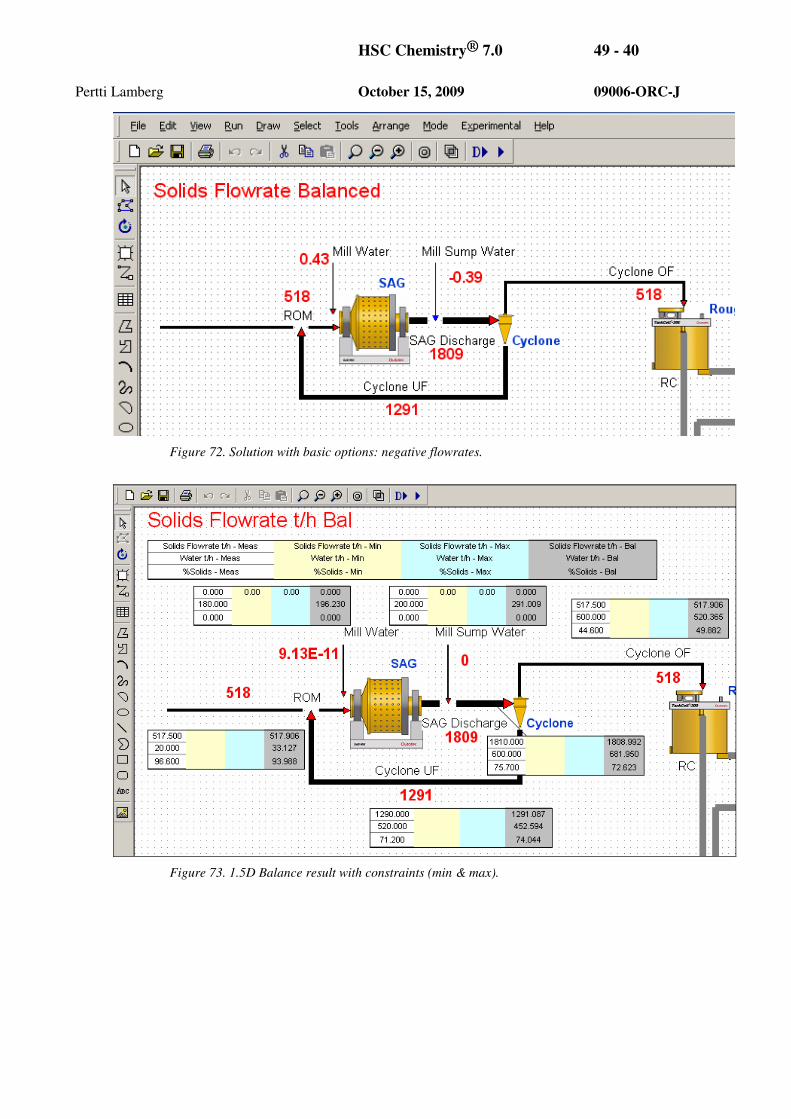
Running the mass balance with default options will give negative solid flowrates for the Mill
Sump Water (Figure 70). Again, we need to use CLS method. Set min and max values for
the “Mill Water” (0 and 0), “Mill Sump Water” (0 and 0). Figure 73 gives the result of the
mass balancing. To draw cumulative passing graphs select Graphics – Cumulative Passing
(Figure 74 and Figure 75).
Figure 68. 1.5D example: ”3 Grinding Survey” of the Copper Circuit . “Vertical” (on the bottom
of the window) indicates that data is vertical, i.e. each sample is a column.

HSC Chemistry® 7.0 49 - 38
Pertti Lamberg October 15, 2009 09006-ORC-J
Figure 69. Select components; uncheck Cu and S in this exercise.

HSC Chemistry® 7.0 49 - 39
Pertti Lamberg October 15, 2009 09006-ORC-J
Figure 70. Selections for the streams to be included in the mass balancing.
Figure 71. Dimension is 1.5D.
HSC Chemistry® 7.0 49 - 40
Pertti Lamberg October 15, 2009 09006-ORC-J
Figure 72. Solution with basic options: negative flowrates.
Figure 73. 1.5D Balance result with constraints (min & max).

HSC Chemistry® 7.0 49 - 41
Pertti Lamberg October 15, 2009 09006-ORC-J
Figure 74. Studying result as cumulative passing graph.
Figure 75. Cumulative passing graph.
49.6. Example 5 – 2D Chemical components
2D example can be found on the sheet “7 2D with ERRORS” in the vary same Copper
Circuit flowsheet (Figure 76). Activate the sheet and press
-button. In the second window uncheck the water
streams (Figure 77). Other options you can leave as default (i.e. Skip Wizard). Run the 1D
mass balance (Figure 78); in the example NNLS method was used. Once you are happy with
the 1D balance, change the dimension to 2D (Figure 79) and run the balance again. Now 2D

HSC Chemistry® 7.0 49 - 42
Pertti Lamberg October 15, 2009 09006-ORC-J
balance is solved using 1D balance as constraints (Figure 80). Check the difference between
balanced and measured with the partity chart (Figure 81, Figure 82). Finally save the results
into Experimental Data (Figure 83, Figure 84)
Figure 76. 2D example.
Figure 77. Uncheck Mill Water and Mill Sump Water in the mass balancing.

HSC Chemistry® 7.0 49 - 43
Pertti Lamberg October 15, 2009 09006-ORC-J
Figure 78. Runnin 1D mass balance with NNLS method.
Figure 79. Click 2D.

HSC Chemistry® 7.0 49 - 44
Pertti Lamberg October 15, 2009 09006-ORC-J
Figure 80. 2D mass balance solved.
Figure 81. Parity Chart.

HSC Chemistry® 7.0 49 - 45
Pertti Lamberg October 15, 2009 09006-ORC-J
Figure 82. Parity Chart, copper assay, measured vs. balanced.
Figure 83. Saving result.

HSC Chemistry® 7.0 49 - 46
Pertti Lamberg October 15, 2009 09006-ORC-J
Figure 84. Result in Experimental Data.
49.7. Example 6 – Multiple Data Sets
Multiple data sets example can be found on the sheet “8 Several Sets” in the vary same
Copper Circuit flowsheet (Figure 85). Activate the sheet and press
-button. Use the default options, i.e. press Skip
Wizard.
In the Data Balance and Reconciliation window select NNLS method. You can change the
other options like standard deviation, sampling error, min and max values, if you like. Press
or button to solve the mass balance. Check the
result and if you are happy you can check what is the balance with other cases: change the
case in the “Case” combo box (Figure 86). In this exercise the standard deviation for the
ROM solids flowrate was set to 0.1.
When you are ready to run all the cases in one go select from the menu “Tools – Solve All
Cases” (Figure 87). Give name for the result sheet (Figure 88) and HSC Sim will create the
sheet and run the balance for all cases. After finishing the mass balance HSC Sim will show
the “Experimental Data”, where you can identify the streams (Figure 89), calculate
recoveries (Figure 90) and adjust formatting (Figure 91, Figure 92).

HSC Chemistry® 7.0 49 - 47
Pertti Lamberg October 15, 2009 09006-ORC-J
Figure 85. Data with several sets; Sheet ”8 Several Sets”.
Figure 86. Changing to second case.

HSC Chemistry® 7.0 49 - 48
Pertti Lamberg October 15, 2009 09006-ORC-J
Figure 87. Solving all cases.
Figure 88. Naming the result sheet.
Figure 89. Identify Streams and …
Figure 90. … calculate the recoveries.

HSC Chemistry® 7.0 49 - 49
Pertti Lamberg October 15, 2009 09006-ORC-J
Figure 91. Formatting the result sheet.
Figure 92. The result.