MAS1403

Quantitative Methods for

Business Management

Revision material for Semester 1

Dr. Daniel Henderson

Semester 1 syllabus

Use this checklist to tick things off as you revise them!

1. Collecting and presenting data

2. Graphical methods for presenting data

• stem–and–leaf plots;

• bar charts and multiple bar charts;

• histograms;

• % relative frequency histograms and polygons;

• ogives (cumulative frequency polygons);

• pie charts;

• time series plots;

• scatterplots.

3. Numerical summaries for data

• measures of location – mean, median and mode;

• measures of spread – range, IQR and variance/standard deviation;

• box and whisker plots.

4. Introduction to probability

5. Conditional probability

6. Decision–making using probability

• Expected Monetary Value;

• decision trees.

7. Discrete probability models

• discrete probability distributions;

• permutations and combinations.

8. More discrete probability models

• the binomial distribution;

• the Poisson distribution.

9. Continuous probability models

• probability density functions;

• the Normal distribution.

10. More continuous probability models

• the uniform distribution;

• the exponential distribution.

2

1 Collecting and presenting data

1.1 Definitions

The quantities measured in a study are called random variables and a particular outcome is called

an observation. A collection of observations is the data. The collection of all possible outcomes is

the population.

We can rarely observe the whole population. Instead, we observe some sub–set of this called

the sample. The difficulty is in obtaining a representative sample.

Data/random variables are of different types:

• Qualitative (i.e. non-numerical)

– Categorical

∗ Outcomes take values from a set of categories, e.g. mode of transport to Uni: {car,

metro, bus, walk, other}.

• Quantitative (i.e. numerical)

– Discrete

∗ Things that are countable, e.g. number of people taking this module.

∗ Ordinal, e.g. response to questionnaire; 1 (strongly disagree) to 5 (strongly agree)

– Continuous

∗ Things that we measure rather than count, e.g. height, weight, time.

1.2 Sampling techniques

This section outlines the key concepts, and main pros and cons, of each type of sampling covered

in this course.

1. Simple random sampling

– Each element in the population is equally likely to be drawn into the sample.

– All elements are “put in a hat” and the sample is drawn from the “hat” at random.

– Advantages – easy to implement; each element has an equal chance of being selected.

– Disadvantages – often don’t have a complete list of the population; not all elements might

be equally accessible; it is possible, purely by chance, to pick an unrepresentative sample.

3

2. Stratified sampling

– We take a simple random sample from each “strata”, or group, within the population. The

sample sizes are usually proportional to the population sizes.

– Advantages – sampling within each stratum ensures that that stratum is properly represented

in the sample; simple random sampling within each stratum has the advantages listed under

simple random sampling above.

– Disadvantages – need information on the size and composition of each group; as with s.r.s.,

we need a list of all elements within each strata.

3. Systematic sampling

– The first element from the population is selected at random, and then every kth item is chosen

after this. This type of sampling is often used in a production line setting.

– Advantages – its simplicity! – and so it’s easy to implement;

– Disadvantages – not completely random; if there is a pattern in the production process it is

easy to obtain a biased sample; only really suited to structured populations.

4. Multi–stage sampling

– The population is divided into geographic areas, and then just one of these areas is selected

(probably randomly). A simple random sample, or some other type of sample, is then taken

from this area.

– Advantages – saves time and cost, since sampling is concentrated within one geographic

area.

– Disadvantages – the sample can be biased of the “stages”, or “geographic areas”, are not

carefully defined.

5. Cluster sampling

– Similar to multi–stage sampling, but this time all the elements within the chosen cluster are

sampled, and the cluster isn’t chosen randomly.

– Advantages – Fairly easy (and cheap) to implement – we just sample everyone within the

chosen cluster!

– Disadvantages – easy to get a biased sample.

6. Judgemental sampling

– The person interested in obtaining the data decides who should be surveyed; for example,

the target population might be 16–25 year old females.

– Advantages – very focussed and aimed at the target population.

– Disadvantages – relies on the judgement of the person conducting the questionnaire/survey,

and so could include elements not within the target population.

4

7. Accessibility sampling

– Here, the most easily accessible elements are sampled.

– Advantages – easy to implement.

– Disadvantages – prone to bias.

8. Quota sampling

– Similar to stratified sampling, but uses judgemental sampling within each strata instead of

random sampling. We sample within each strata until our quotas have been reached.

– Advantages – results can be very accurate as this technique is very targeted.

– Disadvantages – the identification of appropriate quotas can be problematic; this sampling

technique relies heavily on the judgement of the interviewer.

1.3 Frequency tables

Once we have collected our data, often the first stage of any analysis is to present them in a simple

and easily understood way. Tables are perhaps the simplest means of presenting data. You should

know how to construct (and read!) simple frequency tables and relative % frequency tables for

both discrete and continuous data.

1.4 Exam–style questions

1. Explain briefly each of the following forms of sampling:

(a) simple random sampling;

(b) stratified random sampling;

(c) cluster sampling.

2. The table below gives the amounts, in £, spent at a supermarket by a sample of 80 customers.

Construct a frequency table for these data, using class intervals 10 ≤ x < 20, 20 ≤ x < 30,30 ≤ x < 40 and so on. Show frequency, relative frequency and cumulative relative frequency.

40.83 22.10 45.68 39.11 18.92 43.22 37.30 109.97 22.45 42.89

32.95 21.07 41.35 42.54 17.63 19.68 44.62 38.69 66.78 31.99

91.96 25.28 14.82 43.82 44.02 17.31 28.46 28.00 78.28 44.11

29.60 35.34 41.73 65.42 18.65 28.44 45.78 15.99 34.20 35.92

52.03 50.46 58.34 55.03 48.17 43.82 57.77 36.36 53.64 95.75

23.62 34.05 14.47 11.60 23.05 84.30 38.31 41.08 39.47 32.51

32.59 23.58 17.00 25.41 16.78 37.91 80.59 47.32 21.71 28.89

37.97 22.84 47.24 31.34 63.91 81.94 29.06 26.41 36.01 50.78

5

3. (a) A toy company is to be inspected for the quality and safety of the teddy bears it produces.

The inspection team takes a sample of teddy bears from the production line by choosing the

first teddy bear at random, and then selecting every 100th teddy bear thereafter. What form

of sampling are the team using?

(b) Give one disadvantage of the sampling technique described in part (a).

(c) Another inspection team is to investigate the quality of the company’s dolls’ houses. In a

single working day, the toy company produces 100 houses for Barbie dolls, 200 houses for

Cindy dolls and 300 houses for raggy dolls. Suggest a suitable form of sampling to check

the quality of dolls’ houses produced, and suggest how the inspection team might obtain a

sample of size 300.

6

2 Graphical methods for presenting data

Once we have collected our data, often the best way to summarise this data is through an appropri-

ate graph. Graphs are more eye–catching than tables, and give us an “at–a–glance” picture of our

data without too much thought!

2.1 Stem–and–leaf plots

Consider the following data: 11, 12, 9, 15, 21, 25, 19, 8. The first step is to decide on interval widths

– one obvious choice would be to go up in 10s. This would give a stem unit of 10 and a leaf unit

of 1. The stem and leaf plot is constructed as below.

0 8 9

1 1 2 5 9

2 1 5

Stem Leaf

n = 8, stem unit = 10, leaf unit = 1.

Some notes on stem–and–leaf plots.

– Always show the stem units and the leaf units.

– The stem unit will usually be either 10 or 1; the corresponding unit for the leaves is usually

1 and 0.1.

– If your sample size is large, you can split each row into two (i.e. 10–14 and 15–19).

– If you have observations recorded to 2 d.p., always round down to obtain values to 1 d.p.

2.2 Bar charts and multiple bar charts

These are relatively simple to draw. Just be careful with your scale on the y–axis – make sure it

covers the entire range of frequencies! And make sure you leave clear gaps between the bars!

2.3 Histograms

Simple frequency histograms can be thought of as “bar charts for continuous data”. The only

difference is that you need to split the range of your data up into “chunks” or class intervals, and

you should aim for between 10–15 of these. Once you’ve done this, simply count the number of

observations within each “chunk”, and then draw your graph! Remember, unlike bar charts, there

are no gaps between the bars in a histogram.

2.4 Percentage relative frequency histograms and polygons

These are just like histograms, but we convert the frequencies into percentages and the heights of

the bars now correspond to percentages instead of frequencies. These are useful for illustrating the

relative differences between two groups because both are put “onto the same scale”.

7

Percentage relative frequency polygons are constructed in exactly the same way, but now the mid–

points of the top of each bar are now connected with straight lines to form a polygon. These are

particularly useful for comparing two or more groups (more than two bar charts superimposed

could get very messy!).

2.5 Ogives

– Construct a percentage relative frequency table for your data.

– Add a “cumulative” column by adding up the percentages as you go along.

– Plot the upper end–point of each class interval against the cumulative value.

2.6 Pie charts, time series plots and scatterplots

These plots are all relatively simple to construct. You should know how to make appropriate com-

ments on all plots you draw, but there are some things you should look out for with time series

plots and scatterplots in particular.

For time series plots, look out for trend and seasonal cycles in the data. Also look out for any

outliers.

For scatterplots, is there a linear association between the two variables? If so, is this positive

(“uphill”) or negative (“downhill”)? Is the association strong? Or maybe moderate or weak?

2.7 Exam–style questions

1. The number of new orders received by a company over the last fourteen working days were

recorded as follows:

31 20 25 19 35 36 18 17 68 20 43 21 27 9

Display these data in a stem–and–leaf diagram, and comment.

2. The following table contains some data on the weekly household expenditure on food for 200

families.

Interval Frequency Interval Frequency

40 – 60 4 160 – 180 22

60 – 80 12 180 – 200 18

80 – 100 18 200 – 220 6

100 – 120 28 220 – 260 8

120 – 140 48 260 – 280 4

140 – 160 32

Draw a percentage relative frequency polygon for these data, and comment.

8

3 Numerical summaries for data

When summarising data numerically, you should use both a measure of location and a measure of

spread. A measure of location is a value which is “typical” of the observations in our sample, and

a measure of spread quantifies how “spread out” (or how “fat”) our data are.

3.1 Measures of location

1. The mean

The sample mean is given by the formula

x̄ =1

n

n∑

i=1

xi,

which, put more simply, means “add them up and divide by how many you’ve got”.

2. The median

This is just the observation “in the middle”, when the data are put into order from smallest to

largest:

median =

(

n+ 1

2

)th

smallest observation.

If the sample size (n) is an even number then this simplifies to:

median = average of the(n

2

)th

and the(n

2+ 1

)th

smallest observations.

The median is often used if the dataset has an asymmetric profile, since it is not distorted by ex-

treme observations (“outliers”).

3. The mode

The mode is simply the most frequently occurring observation. The mode is easy to obtain from

a stem–and–leaf plot or a bar–chart. The modal class is easily obtained from a grouped frequency

table or a histogram.

3.2 Measures of spread

1. The range

Remember, measures of spread attempt to quantify how “spread out” our data are. The range is

arrived at quite intuitively from this definition – it is just the largest value minus the smallest value,

which gives the “range” occupied by our data.

2. The inter–quartile range

The IQR measures the range of the middle half of the data, and so is less affected by extreme

observations. It is given by Q3−Q1, where

Q1 =(n+ 1)

4th smallest observation

Q3 =3(n+ 1)

4th smallest observation.

9

3. The variance and standard deviation

The variance can be thought of as “the average squared distance from the mean”, and is given by

s2 =1

n− 1

n∑

i=1

(xi − x̄)2 .

The following formula is easier for calculations

s2 =1

n− 1

{

n∑

i=1

x2

i− (n× x̄2)

}

.

In practice most people simply use the Statistics mode on their calculator (mode SD or Stat). [If

you haven’t already done so, you should purchase a University-approved calculator (e.g. Casio

fx-83GT PLUS) and learn how to use the Statistics mode; help will be given with this during tuto-

rials in Semester 2.]

The standard deviation is just the square root of the variance, and is often preferred as it is in

the “original units of the data”.

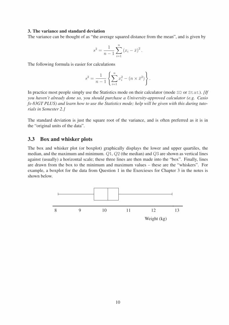
3.3 Box and whisker plots

The box and whisker plot (or boxplot) graphically displays the lower and upper quartiles, the

median, and the maximum and minimum. Q1, Q2 (the median) and Q3 are shown as vertical lines

against (usually) a horizontal scale; these three lines are then made into the “box”. Finally, lines

are drawn from the box to the minimum and maximum values – these are the “whiskers”. For

example, a boxplot for the data from Question 1 in the Exercieses for Chapter 3 in the notes is

shown below.

Weight (kg)

8 9 10 11 12 13

10

3.4 Exam–style questions

1. The number of new orders received by a company over the last ten working days were recorded

as follows:

20 25 19 18 17 20 43 21 27 9

Calculate the mean, median, and standard deviation for these data.

2. The following data are total monthly sales (May 2013, in thousands of pounds) for an Italian

pizza chain in ten university towns in England:

117 62 118 120 169 157 202 88 104 149

Draw a box and whisker plot for these data, and comment. What is the inter–quartile range?

11

4 Introduction to probability

4.1 Definitions

An experiment is an activity where we do not know for certain what will happen, but we will

observe what happens. An outcome is one of the possible things that can happen. The sample

space is the set of all possible outcomes. An event is a set of outcomes.

Probabilities are usually expressed in terms of fractions, decimal numbers or percentages.

All probabilities are measured on a scale ranging from zero to one. The probabilities of most

events lie strictly between zero and one as an event with probability zero is an impossible event

and an event with probability one is a certain event.

Two events are said to be mutually exclusive if both cannot occur simultaneously. Two events

are said to be independent if the occurrence of one does not affect the probability of the other

occurring.

4.2 Measuring probability

1. Classical interpretation

If all possible outcomes are “equally likely” then we can adopt the classical approach to measuring

probability. For example, if we tossed a fair coin, there are only two possible outcomes – a head

or a tail – both of which are equally likely, and hence

P (Head) =1

2and P (Tail) =

1

2.

In general, calculations follow from the formula

P (Event) =Total number of outcomes in which event occurs

Total number of possible outcomes.

2. Frequentist interpretation

When the outcomes of an experiment are not equally likely, we can conduct experiments to give

us some idea of how likely the different outcomes are. We perform the same experiment a large

number of times and observe the outcome. By conducting experiments the probability of an event

can easily be estimated using the following formula:

P (Event) =Number of times an event occurs

Total number of times experiment performed.

3. Subjective interpretation

As the name suggests, probabilities within this framework are formulated subjectively using an

individual’s (sometimes expert) opinion. When we board an aeroplane, we judge the probability of

it crashing to be sufficiently small that we are happy to undertake the journey. Similarly, the odds

given by bookmakers on a horse race reflect people’s beliefs about which horse will win.

12

4.3 Laws of Probability

Multiplication Law

The probability of two independent events A and B both occurring can be written as

P (A and B) = P (A)× P (B).

Addition Law

The addition law describes the probability of any of two or more events occurring. The addition

law for two events A and B is

P (A or B) = P (A) + P (B)− P (A and B).

This describes the probability of either event A or event B happening.

4.4 Exam–style questions

1. In the U.K., 65% of small businesses conduct market research before launching a new product;

half of small businesses use a pilot study to check how successful a new product will be before

launching it; and 20% of small businesses use both market research and a pilot study.

(a) Find the probability that a randomly chosen small business in the U.K. uses either market

research or a pilot study before launching their product.

(b) What percentage of small businesses in the U.K. launch their products without any pre–

launch research?

2. A chain of clothes retailers has conducted an equal opportunities audit. The number of male

and female employees in three types of job – Store Manager, Senior Sales Person and Sales

Person – was recorded, the results of which are shown in the table below.

Male Female Total

Store Manager 20 4 24

Senior Sales Person 100 140 240

Sales Person 120 202 322

Total 240 346 586

(a) What is the probability that a randomly chosen employee from this survey is male?

(b) What is the probability that a Store Manager is female?

(c) What is the probability that a randomly selected female from this survey is either a Sales

Person or a Senior Sales Person?

13

5 Conditional probability and tree diagrams

5.1 Conditional probability

Consider two events A and B. We write

P (B|A)

for the probability of B given that A has already happened. We describe P (B|A) as the conditional

probability of B given A. This gives the following extension to the multiplication rule given

previously:

P (A and B) = P (A)× P (B|A)

5.2 Tree diagrams

Tree diagrams are simple, clear ways of presenting probabilistic information. Suppose we have a

biased coin, with P (Head) = 0.75. Then the following tree diagram displays all outcomes, along

with their associated probabilities, for two consecutive flips of the coin:

H

H

HT

T

T0.75

0.75

0.75

0.25

0.25

0.25

0.75× 0.75 = 0.5625

0.75× 0.25 = 0.1875

0.25× 0.75 = 0.1875

0.25× 0.25 = 0.0625

5.3 Exam–style question

The probability that a machine needs a new belt is 0.55. If the machine needs a new belt then the

probability that it will need a new motor is 0.4. However, if the machine doesn’t need a new belt

then the probability that it will need a new motor is only 0.3.

(a) Find the probability that the machine needs a new belt and a new motor.

(b) Find the conditional probability that the machine needs a new belt given that it needs a new

motor.

14

6 Decision–making using probability

6.1 Expected Monetary Value

The Expected Monetary Value (EMV) of a single event is simply the probability of that event

multiplied by its monetary value. In general,

EMV =∑

P (Event)× Monetary value of Event

where the sum is over all possible events. EMV is often combined with decision trees, examples

of which are given in the following questions.

6.2 Decision trees

Decision trees are best revised via an example – see the exam–style question below.

6.3 Exam–style question

The manager of a small business has the opportunity to buy a fixed quantity of a new product and

offer it for sale for a limited time.

The decision to buy the product and offer it for sale would involve a fixed cost of £150,000. The

amount that would be sold is uncertain but the manager’s beliefs are expressed as follows.

• There is a probability of 0.3 that sales will be “poor” with an income of £80,000.

• There is a probability of 0.5 that sales will be “medium” with an income of £160,000.

• There is a probability of 0.2 that sales will be “good” with an income of £240,000.

For an additional fixed cost of £20,000, the product can be sold for a trial period before a final

decision is made. No income is made from this trial. The result of the trial will be “poor” with

probability 0.33, “medium” with probability 0.40 or “good” with probability 0.27. Knowing the

outcome of the trial changes the probabilities for the main sales project:

Main sales probabilities

Trial outcome Poor Medium Good

Poor 0.7 0.2 0.1

Medium 0.2 0.6 0.2

Good 0.1 0.2 0.7

The manager will make decisions on the basis of expected monetary value.

(a) Draw a decision tree for this problem.

(b) Find the expected monetary value of a decision to go ahead with the product without a trial.

(c) Complete the solution of the decision problem and determine the optimal course of action

for the company.

15

7 Discrete probability models

7.1 Probability distributions

The probability distribution of a discrete random variable X is the list of all possible values Xcan take and the probabilities associated with them. For example, if the random variable X is the

outcome of a roll of a die then the probability distribution for X is:

k 1 2 3 4 5 6 Sum

P (X = k) 1/6 1/6 1/6 1/6 1/6 1/6 1

For a discrete random variable the probabilities of each possible value sum up to 1.

7.2 Permutations and combinations

The number of ways of choosing r objects out of n, when the ordering matters, is given by

nPr =n!

(n− r)!,

where

n! = n× (n− 1)× (n− 2)× (n− 3)× · · · × 3× 2× 1.

Sometimes the ordering of the chosen numbers is not important – all that’s important is that we get

the correct numbers! If this is the case, the number of ways of choosing r objects out of n is given

by

nCr =n!

r!(n− r)!.

An example of where ordering is not important is the national lottery – we don’t care what order

the numbers come out in, as long as our numbers are there! For the jackpot, the number of ways

of choosing 6 correct numbers from all 59 is given by 59C6 = 45057474.

16

8 More discrete probability models

8.1 The binomial distribution

Suppose the following statements hold:

• There are a fixed number of trials (n).

• There are only two possible outcomes for each trial (‘success’ or ‘failure’).

• There is a constant probability of ‘success’, p.

• The outcome of each trial is independent of any other trial.

Then the number of successes, X , follows a binomial distribution.

We write X ∼ Bin(n, p), and

P (X = r) = nCr × pr × (1− p)n−r, r = 0, 1, . . . , n.

If X ∼ Bin(n, p), then its mean and variance are

E[X] = n× p and

Var(X) = n× p× (1− p).

8.2 The Poisson distribution

Suppose the following hold:

• Events occur independently, at a constant rate (λ);

• There is no natural upper limit to the number of events.

Then the number of events, X , occurring in a given interval, has a Poisson distribution.

We write X ∼ Po(λ), and

P (X = r) =λre−λ

r!, r = 0, 1, . . .

If X ∼ Po(λ), then its mean and variance are

E[X] = λ and

Var(X) = λ.

17

8.3 Exam–style questions

1. A new Mercedes–Benz car franchise forecasts that it will sell around three of its most expensive

models each day.

(a) What probability distribution might be reasonable to use to model the number of cars sold

each day?

(b) What is the expected number and standard deviation of the number of cars sold each day?

(c) What is the probability that no cars are sold on a particular day?

2. An operator at a call centre has 20 calls to make in an hour. History suggests that they will be

answered 55% of the time. Let X be the number of answered calls in an hour.

(a) What probability distribution does X have?

(b) What is the mean and standard deviation of X?

(c) Calculate the probability of getting a response exactly 9 times.

(d) Calculate the probability of getting fewer than 2 responses.

18

9 Continuous probability models

9.1 The Normal distribution

The Normal distribution is possibly the best–known and most–used continuous probability dis-

tribution. The Normal distribution has two parameters: the mean, µ, and the standard deviation, σ.

Its probability density function (pdf) has a “bell shaped” profile:

x

f(x)

µµ− 2σ µ+ 2σµ− 4σ µ+ 4σ

If a random variable X has a Normal distribution with mean µ and variance σ2, then we write

X ∼ N(

µ, σ2)

.

The standard Normal distribution, usually denoted by Z, has a mean of zero and a variance of

1, and we have tables of probabilities for this particular Normal distribution. Any Normally dis-

tributed random variable X can be transformed into the standard Normal distribution using the

formula:

Z =X − µ

σ;

once we’ve performed this “slide–squash” transformation, we obtain probabilities by reference

to statistical tables. Don’t forget, tables give “less than” probabilities. So, for a “greater than”

probability, subtract the “less than” probability found in the tables from 1. Similarly, we can use

tables to find the probability that our random variable lies between two values.

9.2 Exam–style question

A call centre’s declared policy is to respond to calls within 50 seconds. In reality they respond

according to a Normal distribution with a mean of 60 seconds and a standard deviation of 10

seconds.

(a) What proportion of calls receive a late response?

(b) What proportion of calls are answered between 50 and 70 seconds?

19

Probability Tables for the Standard Normal Distribution

The table contains values of P (Z ≤ z), where Z ∼ N(0, 1).

z -0.09 -0.08 -0.07 -0.06 -0.05 -0.04 -0.03 -0.02 -0.01 0.00

-2.9 0.0014 0.0014 0.0015 0.0015 0.0016 0.0016 0.0017 0.0018 0.0018 0.0019

-2.8 0.0019 0.0020 0.0021 0.0021 0.0022 0.0023 0.0023 0.0024 0.0025 0.0026

-2.7 0.0026 0.0027 0.0028 0.0029 0.0030 0.0031 0.0032 0.0033 0.0034 0.0035

-2.6 0.0036 0.0037 0.0038 0.0039 0.0040 0.0041 0.0043 0.0044 0.0045 0.0047

-2.5 0.0048 0.0049 0.0051 0.0052 0.0054 0.0055 0.0057 0.0059 0.0060 0.0062

-2.4 0.0064 0.0066 0.0068 0.0069 0.0071 0.0073 0.0075 0.0078 0.0080 0.0082

-2.3 0.0084 0.0087 0.0089 0.0091 0.0094 0.0096 0.0099 0.0102 0.0104 0.0107

-2.2 0.0110 0.0113 0.0116 0.0119 0.0122 0.0125 0.0129 0.0132 0.0136 0.0139

-2.1 0.0143 0.0146 0.0150 0.0154 0.0158 0.0162 0.0166 0.0170 0.0174 0.0179

-2.0 0.0183 0.0188 0.0192 0.0197 0.0202 0.0207 0.0212 0.0217 0.0222 0.0228

-1.9 0.0233 0.0239 0.0244 0.0250 0.0256 0.0262 0.0268 0.0274 0.0281 0.0287

-1.8 0.0294 0.0301 0.0307 0.0314 0.0322 0.0329 0.0336 0.0344 0.0351 0.0359

-1.7 0.0367 0.0375 0.0384 0.0392 0.0401 0.0409 0.0418 0.0427 0.0436 0.0446

-1.6 0.0455 0.0465 0.0475 0.0485 0.0495 0.0505 0.0516 0.0526 0.0537 0.0548

-1.5 0.0559 0.0571 0.0582 0.0594 0.0606 0.0618 0.0630 0.0643 0.0655 0.0668

-1.4 0.0681 0.0694 0.0708 0.0721 0.0735 0.0749 0.0764 0.0778 0.0793 0.0808

-1.3 0.0823 0.0838 0.0853 0.0869 0.0885 0.0901 0.0918 0.0934 0.0951 0.0968

-1.2 0.0985 0.1003 0.1020 0.1038 0.1056 0.1075 0.1093 0.1112 0.1131 0.1151

-1.1 0.1170 0.1190 0.1210 0.1230 0.1251 0.1271 0.1292 0.1314 0.1335 0.1357

-1.0 0.1379 0.1401 0.1423 0.1446 0.1469 0.1492 0.1515 0.1539 0.1562 0.1587

-0.9 0.1611 0.1635 0.1660 0.1685 0.1711 0.1736 0.1762 0.1788 0.1814 0.1841

-0.8 0.1867 0.1894 0.1922 0.1949 0.1977 0.2005 0.2033 0.2061 0.2090 0.2119

-0.7 0.2148 0.2177 0.2206 0.2236 0.2266 0.2296 0.2327 0.2358 0.2389 0.2420

-0.6 0.2451 0.2483 0.2514 0.2546 0.2578 0.2611 0.2643 0.2676 0.2709 0.2743

-0.5 0.2776 0.2810 0.2843 0.2877 0.2912 0.2946 0.2981 0.3015 0.3050 0.3085

-0.4 0.3121 0.3156 0.3192 0.3228 0.3264 0.3300 0.3336 0.3372 0.3409 0.3446

-0.3 0.3483 0.3520 0.3557 0.3594 0.3632 0.3669 0.3707 0.3745 0.3783 0.3821

-0.2 0.3859 0.3897 0.3936 0.3974 0.4013 0.4052 0.4090 0.4129 0.4168 0.4207

-0.1 0.4247 0.4286 0.4325 0.4364 0.4404 0.4443 0.4483 0.4522 0.4562 0.4602

0.0 0.4641 0.4681 0.4721 0.4761 0.4801 0.4840 0.4880 0.4920 0.4960 0.5000

z 0.00 0.01 0.02 0.03 0.04 0.05 0.06 0.07 0.08 0.09

0.0 0.5000 0.5040 0.5080 0.5120 0.5160 0.5199 0.5239 0.5279 0.5319 0.5359

0.1 0.5398 0.5438 0.5478 0.5517 0.5557 0.5596 0.5636 0.5675 0.5714 0.5753

0.2 0.5793 0.5832 0.5871 0.5910 0.5948 0.5987 0.6026 0.6064 0.6103 0.6141

0.3 0.6179 0.6217 0.6255 0.6293 0.6331 0.6368 0.6406 0.6443 0.6480 0.6517

0.4 0.6554 0.6591 0.6628 0.6664 0.6700 0.6736 0.6772 0.6808 0.6844 0.6879

0.5 0.6915 0.6950 0.6985 0.7019 0.7054 0.7088 0.7123 0.7157 0.7190 0.7224

0.6 0.7257 0.7291 0.7324 0.7357 0.7389 0.7422 0.7454 0.7486 0.7517 0.7549

0.7 0.7580 0.7611 0.7642 0.7673 0.7704 0.7734 0.7764 0.7794 0.7823 0.7852

0.8 0.7881 0.7910 0.7939 0.7967 0.7995 0.8023 0.8051 0.8078 0.8106 0.8133

0.9 0.8159 0.8186 0.8212 0.8238 0.8264 0.8289 0.8315 0.8340 0.8365 0.8389

1.0 0.8413 0.8438 0.8461 0.8485 0.8508 0.8531 0.8554 0.8577 0.8599 0.8621

1.1 0.8643 0.8665 0.8686 0.8708 0.8729 0.8749 0.8770 0.8790 0.8810 0.8830

1.2 0.8849 0.8869 0.8888 0.8907 0.8925 0.8944 0.8962 0.8980 0.8997 0.9015

1.3 0.9032 0.9049 0.9066 0.9082 0.9099 0.9115 0.9131 0.9147 0.9162 0.9177

1.4 0.9192 0.9207 0.9222 0.9236 0.9251 0.9265 0.9279 0.9292 0.9306 0.9319

1.5 0.9332 0.9345 0.9357 0.9370 0.9382 0.9394 0.9406 0.9418 0.9429 0.9441

1.6 0.9452 0.9463 0.9474 0.9484 0.9495 0.9505 0.9515 0.9525 0.9535 0.9545

1.7 0.9554 0.9564 0.9573 0.9582 0.9591 0.9599 0.9608 0.9616 0.9625 0.9633

1.8 0.9641 0.9649 0.9656 0.9664 0.9671 0.9678 0.9686 0.9693 0.9699 0.9706

1.9 0.9713 0.9719 0.9726 0.9732 0.9738 0.9744 0.9750 0.9756 0.9761 0.9767

2.0 0.9772 0.9778 0.9783 0.9788 0.9793 0.9798 0.9803 0.9808 0.9812 0.9817

2.1 0.9821 0.9826 0.9830 0.9834 0.9838 0.9842 0.9846 0.9850 0.9854 0.9857

2.2 0.9861 0.9864 0.9868 0.9871 0.9875 0.9878 0.9881 0.9884 0.9887 0.9890

2.3 0.9893 0.9896 0.9898 0.9901 0.9904 0.9906 0.9909 0.9911 0.9913 0.9916

2.4 0.9918 0.9920 0.9922 0.9925 0.9927 0.9929 0.9931 0.9932 0.9934 0.9936

2.5 0.9938 0.9940 0.9941 0.9943 0.9945 0.9946 0.9948 0.9949 0.9951 0.9952

2.6 0.9953 0.9955 0.9956 0.9957 0.9959 0.9960 0.9961 0.9962 0.9963 0.9964

2.7 0.9965 0.9966 0.9967 0.9968 0.9969 0.9970 0.9971 0.9972 0.9973 0.9974

2.8 0.9974 0.9975 0.9976 0.9977 0.9977 0.9978 0.9979 0.9979 0.9980 0.9981

2.9 0.9981 0.9982 0.9982 0.9983 0.9984 0.9984 0.9985 0.9985 0.9986 0.9986

20

10 More continuous probability distributions

10.1 The uniform distribution

The uniform distribution is the most simple continuous distribution. As the name suggests, it

describes a variable for which all possible outcomes are equally likely. If the random variable Xfollows a Uniform distribution, we write

X ∼ U(a, b).

Probabilities can be calculated using the formula

P (X ≤ x) =

0 for x < ax− a

b− afor a ≤ x ≤ b

1 for x > b,

and the mean and variance are given by

E[X] =a+ b

2, Var(X) =

(b− a)2

12.

10.2 The exponential distribution

The exponential distribution is another common distribution that is used to describe continuous

random variables. It is often used to model lifetimes of products and times between “random”

events such as arrivals of customers in a queueing system or arrivals of orders. The distribution

has one parameter, λ. If our random variable X follows an exponential distribution, then we say

X ∼ Exp(λ).

Probabilities can be calculated using

P (X ≤ x) =

{

1− e−λx for x ≥ 0

0 for x < 0,

and the mean and variance are given by

E[X] =1

λ, Var(X) =

1

λ2.

21

10.3 Exam–style questions

1. A local authority is responsible for a stretch of road 3km long through a town. A gas main runs

along the length of the road. The gas company has requested permission to dig up the road in

one place but has neglected to tell the authority exactly where.

(a) Let Y be the distance of the gas works from one end of the road. Sketch the pdf of Y .

(b) What distribution does Y take?

(c) The stretch of road between 1.5 and 2.75 kilometres from one end goes through the town

centre and gas works there would cause severe disruption. What is the probability that this

happens?

2. The time (in minutes) between uses of a vending machine is modelled as an exponential distri-

bution with rate 0.2.

(a) What is the mean time between uses?

(b) What is the probability that there is a gap of more than 10 minutes between uses?

22

Data type Distribution Notation/ Formula Mean Variance

parameters

Binomial X ∼ Bin(n, p) P (X = r) = nCrpr(1− p)n−r n× p n× p× (1− p)

Discrete

Poisson X ∼ Po(λ) P (X = r) = λre−λ

r!λ λ

Normal X ∼ N(µ, σ2) P (X ≤ x) = P(

Z ≤x− µσ

)

, µ σ2

then use tables

Continuous Exponential X ∼ Exp(λ) P (X ≤ x) = 1− e−λx 1/λ 1/λ2

Uniform X ∼ U(a, b) P (X ≤ x) = x− ab− a

a+ b2

(b− a)2

12