Marriage, Employment and Inequality of Women's Lifetime Earned

Marriage, Employment and Inequality of Women’s Lifetime Earned Income

Chinhui Juhn University of Houston and NBER

[email protected]

Kristin McCue U.S. Census Bureau

[email protected]

September 2011

Abstract: Using Current Population Surveys and Survey of Income and Program Participation data matched to Social Security earnings records, we summarize changes in marital histories for different birth cohorts of women and project the associated changes in women’s own lifetime earnings and in spousal earnings. We find that the gap in lifetime earnings between married and single women appears to have essentially closed for less educated women while a small differential still exists for more educated women. The earnings gap across education categories has increased rapidly in terms of women’s own lifetime earnings. The level of earnings inequality across education categories is higher when marriage and husbands’ earnings is taken into account although the increase is less pronounced. Lifetime earnings of married college- educated women diverged most dramatically from those of less educated single women.

JEL Classification: J12, J16, J22, J31

Any opinions and conclusions expressed herein are those of the authors and do not necessarily represent the views of the U.S. Census Bureau. All results have been reviewed to ensure that no confidential information is disclosed. This research was supported by the U.S. Social Security Administration through grant #5 RRC08098400-03-00 to the National Bureau of Economic Research as part of the SSA Retirement Research Consortium. The findings and conclusions expressed are solely those of the authors and do not represent the views of SSA, any agency of the Federal Government, or the NBER.

2

I. Introduction

Over the past four decades, changes in both marriage and women’s employment have reduced

the economic importance of traditional families in which the husband works predominantly

outside of the home and the wife works and provides child care in the home. For example,

among women who are 18-60 years old, the fraction who are currently living with a spouse fell

from 74 percent in 1968 to 54 percent in 2010. At age 35, 6 percent of women reported never

having married in 1968 while up to 19 percent had never married in 2010.1 Over their lifetimes,

both men and women in recent birth cohorts will spend significantly fewer years of their prime

aged adult life in marriage, both because they are less likely to ever marry and because they

marry at a later age (Stevenson and Wolfers (2007)). Moreover, the patterns have not been

uniform across education and skill groups with marriage rates falling more among less educated

groups (Isen and Stevenson (2010), Juhn and McCue (2010)).

While marriage rates have fallen, it is well known that employment rates have increased

for married women and the fraction of households with dual-earners have increased. In addition,

wives of high wage husbands have increased their employment relative to wives of low wage

husbands (Juhn and Murphy (1997), Blau and Kahn (2007)). In this paper, we propose to

examine the impact of changing marital and employment histories on the distribution of lifetime

earnings (both individual and family) for women. We are particularly interested in inequality

and therefore compare lifetime earnings of less and more educated women who have had

different experiences in both marriage and employment. We also want to know how this

inequality across education groups has progressed over time. We therefore compare across birth

cohorts beginning with those born 1936-40 and ending with those born 1966-70.

1 Based on authors’ calculations using the March Current Population Surveys.

3

The novelty of our exercise largely comes from using the Survey of Income and Program

Participation (SIPP) panels matched to Social Security Administration earnings records from

1951-2006. The data allow us to follow an individual woman’s earnings over much of her

lifetime and also to observe her spouse’s earnings for the subset of women who are married

during their SIPP panel.2 Related work in this area (Gustman and Steinmeier (2001), (2011)) use

the Health and Retirement Survey (HRS) matched to Social Security earnings records. In

comparison to these studies, we have a wider range of cohorts to compare.

The question we propose to examine is particularly relevant for considering post-

retirement income security of women since under current rules with spousal benefits, social

security benefits depend on women’s marital histories as well as their individual earnings

histories. Since employment and earnings increased more among married women than single

women, it may be the case that current benefit rules provide limited income security for women

who never marry and have low lifetime earnings. At the same time, current rules may be

providing redundant income protection for women who have high lifetime earnings of their own.

As pointed out by Liebman (2002), the current system redistributes income based on criteria

other than lifetime earnings and has the unintended consequence of redistributing income from

two-earner married households to one-earner married households even though they may be equal

in terms of potential lifetime earnings.

The paper is organized as follows. Section 2 briefly reviews related papers. Section 3

describes the changes in marriage and employment patterns for women in different education

categories. Section 4 reports the main results on lifetime earnings (individual and including

2 We know the entire marital history of a women up to the year of the SIPP survey and characteristics and earnings history of the current spouse although not the characteristics or earnings of previous spouses. For divorced women, we impute earnings of previous husbands using earnings of current husbands (for those women who remarried) and other characteristics as described in the appendix.

4

spouses’ earnings). Section 5 concludes. Description of sample selection and details regarding

various imputation procedures are in the appendix.

II. Related Literature

Our paper is closely related to the literature on family earnings inequality (Cancian,

Danziger, and Gottschalk (1993), Juhn and Murphy (1997), Blundell, Pistaferri, and Preston

(2008)). These papers generally find that the inclusion of wives’ earnings in the consideration of

family earnings, as opposed to individual male earnings, reduce the rise in earnings inequality

observed since the 1980s. In contrast to these studies we use education levels to group women,

as opposed to husbands’ or couples’ earnings, as a better measure of earnings potential. In

addition, many of the previous studies on family earnings inequality focused exclusively on

continuously married couples whereas we explicitly take into account differences in marital

status across women to calculate inequality of lifetime earnings (both their own and including

spouses’ earnings).

A related literature has examined the impact of changing labor force participation of

women on redistribution under the current Social Security tax and benefit schedules. Gustman

and Steinmeier (2001) use the Health and Retirement Survey matched to Social Security

earnings data to compare lifetime earnings, social security taxes paid, and benefits received and

accrued for individuals and for couples. They find that there is a significant amount of

redistribution across individuals in that the lowest earning individuals have the highest benefits

to tax ratio and this ratio declines with lifetime earnings. Much of this redistribution occurs

within households, however, from high earning husbands to their non-working wives in the form

5

of spousal benefits. When households are the units of observation, they find significantly less

redistribution from high earnings to low-earnings households.

Gustman and Steinmeier (2011) update their earlier work by including a younger cohort

from the HRS. Somewhat surprisingly, they find that despite significantly higher levels of labor

force attachment of wives, not much changed across cohorts and redistribution across households

is limited. Liebman (2002) reaches a similar conclusion using a different dataset, the 1991

Survey of Income and Program Participation matched to Social Security earnings data. He finds

income-related transfers within cohorts account for only a small percent of total benefits paid by

Social Security. Due to the availability of spousal benefits, a large fraction of this redistribution

occurs across demographic categories from single households and two-earner married

households to single-earner married households.

Coronado, Fullerton and Glass (2000) simulate taxes and benefits paid under various

counter-factual scenarios using the Panel Survey of Income Dynamics (PSID). Assigning

potential earnings as opposed to actual earnings to labor market non-participants reduces the

amount of redistribution. In a similar vein, if wives are assigned one-half of combined spousal

earnings, they appear to be significantly less “poor” and the amount of redistribution in the

system is reduced. While we do not directly address the redistributive effects of spousal

benefits, the patterns we document are important in considering the effects of existing or

alternative benefit structures. Relative to these studies, we bring new data to bear that allow us

to compare across multiple cohorts.

III. Trends in Marriage Rates and Earnings

6

We first present an overview of changes in marriage rates among women in different

education categories. In a previous paper, Juhn and McCue (2010), we documented a reversal in

the pattern of marriage across women in different education groups. While the most educated

women were the least likely to ever marry in the earlier birth cohorts, the least educated women

are now the least likely to ever marry among more recent birth cohorts. This pattern is

confirmed in Tables 1 and 2. Table 1 uses 1968-2010 March Current Population Surveys (CPS).

The sample consists of women who were born in 1936-1975.

Table 1 reports the share of women who have ever married by age 35. The table shows

that marriage rates fell for women in all education categories. However, the decline was

particularly large among the least educated, those with a high school education or less. The

share of women who were ever married by age 35 fell from .953 among the 1936-1940 cohort to

.795 among the 1971-1975 cohort. Among college graduates, the share fell by a smaller amount

from .917 to .836.

Table 2 reports the share who are currently married at age 35. This table examines not

only the entry into marriage but also the likelihood of divorce by focusing on current marital

status. This alternative marriage variable tells a similar story with marriage rates falling most

rapidly for the least educated women. While divorce rates have increased among all women, the

increase has been no larger among educated women.

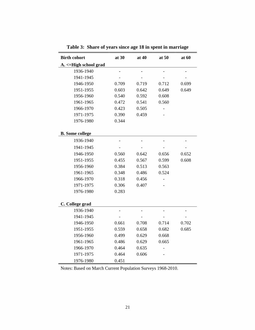
Table 3 presents the cumulative years since age 18 spent in marriage for different cohorts

of women up to the age specified. The table also reports marriage statistics separately for our

three education categories. In the top panel, which refers to women with a high school degree or

less, we find that at age 50 the fraction of years spent in marriage fell from .712 for the 1946-

1950 cohort to .560 for the 1961-1965 cohort. The bottom panel examines college-educated

7

women. At age 50, the share of potential years spent in marriage fell from .714 for the 1946-

1950 birth cohort to .665 for the 1961-1965. The table demonstrates that the decline in time

spent in marriage during prime-aged years declined for all women but much more significantly

for less educated women.

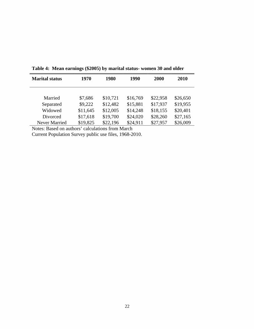
We next turn to the changes in women’s earnings by marital status. Our sample again

comes from the March CPS. We focus on women aged 30 to 60 years old to minimize the age

difference between married and never married women. We include both wage and salary

earnings and self-employment earnings and also include non-participants with zero earnings.

Table 4 reports average earnings by marital status for select years starting with 1970.3 Table 4

shows that in 1970 never-married women earned significantly more than women in all other

categories, especially married women. In 2010, however, married women actually had similar or

even slightly higher earnings than never-married women.

Table 5 shows earnings by marital status for women in different education categories.

Turning to women with a high school degree or less in the top panel, we see that contrary to the

pattern observed in earlier decades, never-married women earn significantly less than married

women in 2010. The reversal is less pronounced among the more educated groups. Among

college women, “never married” women still earn more than married women, $45,807 vs.

$40,002, although there has been considerable catch-up over the four decades. Examining

inequality of women’s earnings across demographic groups, we see that the earnings gap across

marital status has essentially closed by 2010. On the other hand, the earnings gap between

educated and less educated women has widened across all marital status categories.

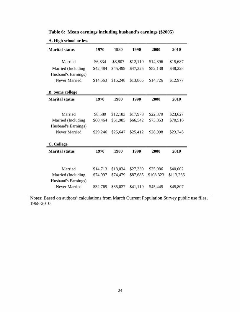
Table 6 contrasts total earnings where we have included husband’s earnings for married

women. For never married single women, total earnings are simply their own earnings. Again 3 We re-code those women who report negative self-employment income to zero earnings in this exercise.

8

we examine women 30-60 years old to minimize the age differences between single and married

women. Table 6 highlights the extent of inequality that exists across marital status and education

categories. For example, while married college-educated women were about on par with “never

married” less educated women (high school grad or dropout) in terms of their own earnings in

1970, when we add in husband’s earnings, total family earnings of college-educated married

women were roughly 5.2 times (74.9/14.5) that of less educated “never married” women.

Moreover, the inequality across these two groups has increased. In 2010, the ratio of family

earnings of college-educated married women was roughly 8.8 times (113.2/12.9) that of less

educated “never married” women.

IV. Women’s Lifetime Earned Income

In the previous section we investigated readily available cross-sectional data (CPS) to

describe changes in women’s marriage and earnings. In this section, we use the Survey of

Income and Program Participation matched to Social Security earnings records (SIPP-SSA) to

construct long-term measures of earnings. The main advantage of these data is that they provide

a long panel data set of women’s earnings (from Social Security records) and marital status

(from SIPP marital histories). There are multiple advantages to panel data for our purposes.

First, while we can estimate average lifetime earnings by birth cohort using repeated cross-

sections, we cannot examine how much it varies across people. While the cross-sectional

variance observed at a particularly point, say age 40, may be a proxy for the variance of lifetime

earnings, it is likely to be poor proxy since transitory earnings variance is a significant

component of the overall variance for women.

9

We use 1951-2006 data on earnings from this panel to examine patterns in the value of

accumulated earnings over women’s lifetimes. The estimates discount future earnings at a rate

of 2 percent, and the value of earnings is deflated by the Personal Consumption Expenditures

index to put them in 2006 dollars. For women who did not attend any college, we accumulate

earnings starting at age 18, while we use 20 as a starting age for those with some college, and 22

for those with at least a college degree.

For younger cohorts who are likely to still be in the labor force for years after 2006, we

base projections past 2006 on the shape of earnings profiles at older ages for earlier cohorts. We

estimate these profiles by running education-group specific fixed-effects regressions of the log of

the discounted value of accumulated earnings on controls for experience, marital status, presence

of children, birth cohort, and interactions among these variables. Details of the methodology are

described in the appendix. In the current draft we do not include measures of the uncertainty

associated with our estimates. To do so we need to capture both the uncertainty arising through

the use of a sample and that added on by our imputation of marital status and earnings in years

that we do not observe. We plan to use multiple imputation methods to estimate standard errors

and confidence intervals in our next draft.

Clearly, projections to age 60 for recent cohorts are at best suggestive of what might

happen, so we present estimates at age 45 as well. For the age 45 projections, the information on

earnings comes only from actual earnings for the first five birth cohorts, and comes primarily

from observed earnings for the sixth. Members of the most recent birth cohort were ages 36-40

in 2006, so even for the youngest and most educated group, only the last third of their earnings

are projected, and the shape of that projection is based on earnings profiles for the 1961-1965

cohort. These forecasts for younger cohorts clearly may differ substantially from eventual

10

outcomes, but we think they are useful as an illustration of what one might expect to see if

current trends continue.

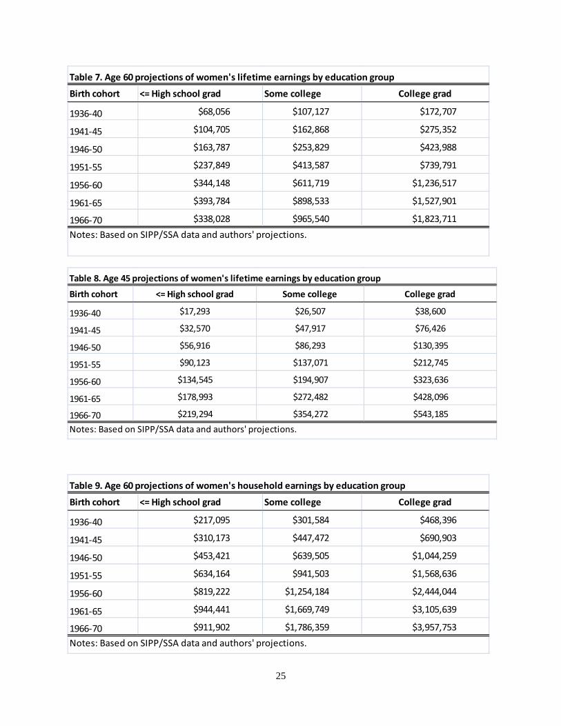
Table 7 presents the age 60 estimates of women’s own present discounted value of

earnings. In all cases, accumulated earnings are greater for more educated women, with college-

educated women earning roughly 60% more than those with some college and 150% more than

those with a high school degree or less in the earliest cohorts. Based on these projections, the

education differential between college grads and those with some college grew modestly across

these cohorts, but both groups had faster growth than did those with no college.

Table 8 presents analogous results using the age 45 projections. Comparing Table 8 to

Table 7, the substantial growth across birth cohorts is evident even using earnings to age 45. But

the pattern of much faster growth in lifetime earnings to age 60 among more educated women is

clearly quite dependent on the accuracy of our projections, as we see very modest divergence

between education groups as of age 45.

We now turn to measures of household earnings, which we define as women’s own

earnings, plus the earnings of their spouse when they are married. We use SIPP marital histories

to determine marital status up to the end of the SIPP panel that a woman was in, and then assign

a probability of being married for years after that. The probability of being married is based on

hazard models of the risk of a marriage ending for women who are married when we last see

them. For those not married when last observed, we instead use hazard models of the risk of a

spell of non-marriage ending through marriage. These estimates condition on age at marriage,

the number of times a woman has been married, and on education and birth cohort. Details are

in the appendix.

11

For the oldest cohorts, roughly 13% of years to age 60 have a forecast of whether a

woman is married rather than actual marital status, but that rises steadily across cohorts and

reaches roughly 70% for the 1966-1970 cohort. The age 45 profiles have almost no imputed

marital status for the first three cohorts, while the share grows from about 5% for the 1951-1955

cohort to about 30% for the most recent cohort.

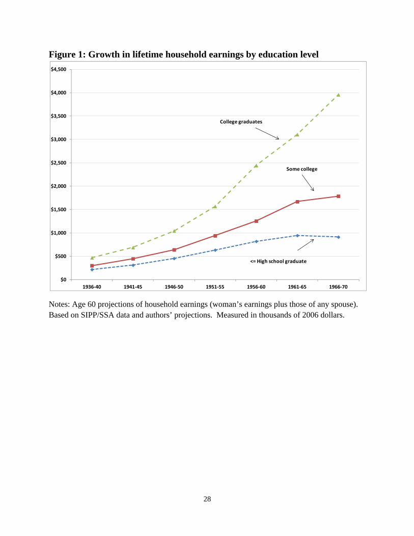
Table 9 gives age 60 projections of household earnings. We see that the discounted value

of household earnings has also grown across birth cohorts, and has grown more for more

educated women. Figure 1 presents these numbers in graphical form. The figure (along with

Table 9) shows the extent of rising inequality across education categories, taking into account

both changes in own earnings, marriage probability, and spouse earnings. For the 1936-40

cohort, college-educated women had discounted lifetime household earnings approximately 2.2

times those of women with high school degree or less. For the 1966-70 cohort, college-educated

women had 4.3 times the household earnings of less educated women. Interestingly, the gap has

not grown as fast in percentage terms as when we consider only their own earnings, reflecting

both less time spent married among more recent cohorts and faster growth in earnings for

married women than for married men. These same general patterns appear in Table 10, which

gives the projections to age 45.

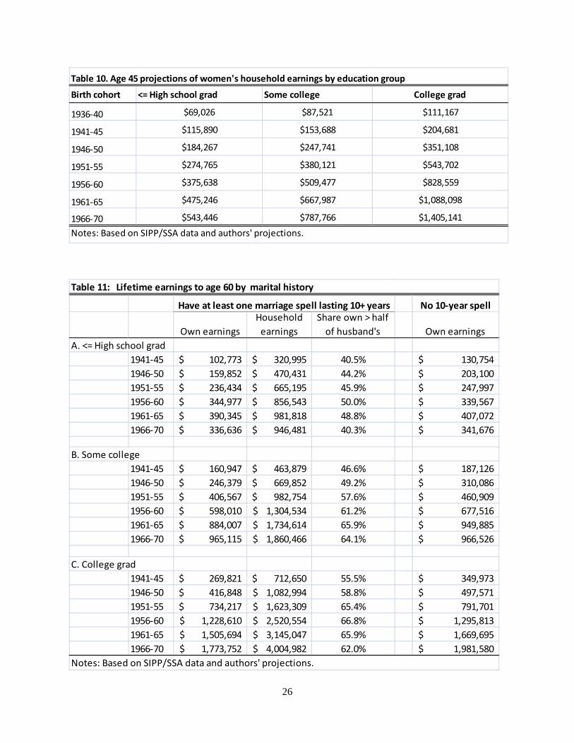
In Table 11, we split our sample into women with at least one marriage that lasts at least

10 years versus those who never marry or are married only for short periods. We are interested

in investigating differences between women for whom spousal earnings are an important source

of income versus those who rely primarily on their own earnings. Using 10 years with one

spouse as a cutoff is in part motivated by current social security benefit rules under which

12

women may receive spousal benefits based on the income of a current or former spouse,

provided the marriage lasted at least 10 years.

The first two columns of Table 11 give own and household lifetime earnings for women

with at least one 10 year marriage. The third column gives the share of women who have

lifetime earnings that are at least half their spouse’s lifetime earnings, to try to capture how

important married women’s own earnings are likely to be relative to husband’s earnings. In all

cases, women with no college are less likely to have discounted lifetime earnings that are at least

half of their husbands’ earnings, and for this group there is no clear trend in this share. Those

with some college had lower shares than women with college degrees in the earlier cohorts but

have very similar probabilities to those with a college degree in the most recent cohorts. This

pattern also shows up in the estimates in Table 12 estimates based on the age 45 projections.

Note that the same group of women are categorized as having a 10+ year marriage spell in

Tables 11 and 12, as it is based on any marriages (or projected marriages) to age 60. The

difference between the two tables is in how many years of earnings are used.

The some-college group has the greatest increase over time and the probabilities look

very similar to those for college graduates in the last two cohorts. The age 45 projections show

lower shares of women having earnings over half of their husbands, likely because years in

which their household included young children would account for a larger share of years to age

45 than to age 60.

The fourth column of both tables gives own earnings for women who either did not marry

or who had only relatively short marriage spells. For all three education groups, this group of

women has higher earnings in the early birth cohorts, but the differential narrows. For those

13

without a college degree, the difference in lifetime earnings associated with marital status is

largely gone for the most recent cohort. For college grads, a modest differential remains. These

trends are illustrated in Figure 2.

As we found in annual measures in Table 5, there is substantial and growing inequality

between the lifetime resources available to married, well-educated women and single women

with no college. For example, in the age 45 projections (Table 12) the 1941-1955 birth cohort of

college-educated women with at least one 10-year marriage spell had about 1.6 times as much in

lifetime earnings as did women with no college and no long marriage spells. But differences

between these two groups in household lifetime earnings were much more dramatic. For that

cohort, the households of college-educated/10+ year marriage spell women had 4.6 times as

much household earnings as those of less educated/no-10-year-spell women. Moreover, the

inequality across these two groups has increased so that for the most recent cohort, that ratio has

grown to 6.4. The differences based on the age 60 projections are more dramatic (though less

reliable)—according to these projections, the ratio grew from about 5.5 to almost 12 across these

cohorts.

V. Conclusion

Over the past four decades the model of a traditional family with a working husband and non-

working wife has become less common. Married women’s employment rates have increased

dramatically at the same time that marriage rates have fallen, especially among the less

educated. In this paper we examine the impact of these developments on women’s lifetime

earnings in terms of both their own earnings as well as household earnings including spouses’

14

earnings. While married and single women may have always been similar in terms of “potential”

earnings, we find that the married women have caught up in terms of actual earnings. While the

earnings gap across marital status has narrowed, inequality across education groups has

increased, reflecting the general trend towards rising inequality across skill groups. College-

educated women as well as women with some college education experienced more growth in

lifetime earnings compared to women with high school degree or less.

When we take into account husbands’ earnings, the level of inequality across education

groups is even higher although the increase is not as dramatic as when considering women’s own

earnings. We find that the most dramatic increase in inequality is across education and marital

status. While in older cohorts they had a modest advantage, more recent cohorts of college-

educated women with long marriage spells have cumulative earnings about 5 times those of less

educated women who spent little or no time in marriage. These developments suggest that going

forward, less educated women will face considerable challenges in terms of retirement security.

On one hand, these women have spent fewer years in marriage relative to their more educated

counterparts and are less likely to qualify for spousal benefits. On the other hand, their own

earnings have not kept up to compensate for the loss of spousal benefits.

15

Data Appendix

Our sample of individuals is drawn from respondents to the 1990-1993, 1996, 2001, and

2004 SIPP panels who provided the information needed to validate matches to Social Security

Administration (SSA) earnings records. Individuals had to be at least 15 years old at the time of

their second SIPP interview to be eligible for inclusion in the matched data.4 For matched

individuals, we have annual earnings for 1951-2006 based on annual summaries of earnings on

jobs recorded in SSA’s Master Earnings File. The primary source of the earnings information is

W-2 records, but self-employment earnings are also included. We include employees’

contributions to deferred compensation plans as part of our earnings measure. We obtain marital

histories, educational attainment, and women’s fertility histories from the SIPP. Age and gender

are based on combined information from the SIPP and SSA sources, with the administrative data

used to fill in missing values.

We use these data to look at cohorts born between 1936 and 1970, following their earnings

over the period 1954-2006 during years in which they were aged 18-60. To determine marital

status at a point in time, we use the marital history information collected in the relevant SIPP

panel with some additional updates from changes in later waves of that panel. This gives us the

information we need on marital status for years leading up to or during the SIPP panel, but not

for the years after the panel is over.

We would like to project women’s own earnings and any earnings that spouses contribute to

household income out to age 60. Doing so requires that we impute information for some ages for

4 The SIPP is a series of short panel surveys in which respondents are surveyed every 4 months to collect detailed information on household members’ income, employment and program participation over the previous months. The surveys also periodically collect detailed information on the demographic characteristics and relationships of household members. Panels have ranged in length from about 2 to 4 years. More detail on the SIPP is available at: http://www.census.gov/hhes/www/sippdesc.html.

16

many sample members. We have developed methods to do so here, but plan to investigate the

sensitivity of our results to alternative methods in future drafts. We describe our methods of

imputing earnings and marital status below.

A complication in examining the earnings of spouses is that we only have information on

both members of couples identified during their SIPP panel. For a woman who divorced before

the start of the SIPP panel, we have information on which prior years she was married, but we

cannot, for example, look at spousal characteristics in those earlier marriages because her

previous spouse is not in the sample. For these women, we impute previous spouses’ earnings as

we describe below. For women with a linked spouse, but with earlier marriages to other men, we

use the current husband’s earnings as a proxy for earlier spouses’ earnings.

A. Top-code Imputations

For the years 1951-1977, the Social Security earnings data are capped at the taxable ceiling.

Over that period, the overall share of workers with earnings above the taxable ceiling ranged

from 15 to 36%.5 Since our sample consists of women and married men, the share affected by

this topcoding is a good bit higher than the overall levels for men, but much lower for women.

For years 1951-1977, we impute earnings above the taxable ceiling in the following manner. We

identify the percentile of the income distribution affected by the topcode for each group (defined

by gender and potential experience) for each year. We use 1978-1980 data to calculate the ratio

of mean earnings above each of those percentiles to the value of income at that percentile of the

1978-1980 distribution, and then apply this ratio to all top-coded earnings observations.

B. Imputing Marital Status for Women Beyond the SIPP Samples

5 See Table 1, CRS (2006).

17

While we observe women’s complete marital histories up to the end of their SIPP panel, we

have no information on their subsequent marital status. For some cohorts of women, it is

possible to estimate marital status using women in the same birth cohort observed in later SIPP

surveys. For younger cohorts, however, we have to extrapolate marriage exit and entry rates

using information on previous birth cohorts. Our basic methodology is the following. For

women for whom we observe actual marital status, we use that information. For women for

whom we do not observe actual marital status we predict marital status in the years we do not

observe them in the following manner. For women who are married when last observed, we

estimate parametric survival models for each education group, assuming a gamma distribution

and using cohort dummies, age of marriage, and dummies for whether this is a first, second or 3+

marriage as regressors. We then predict the probability they remain married in the following

years, conditioning on marital tenure at the point their marital status is last observed.

Analogously, for women who are not married in the last period we observe them, we

estimate similar survival models for the non-marriage spell. We estimate models separately for

our three education groups, using cohort dummies and more detailed education dummies as

covariates. We estimate these models separately for never married women, and treat those spells

as dating from age 18 For women with previous marriage spells, we also include age at which

the current non-marriage spell started and dummies for whether they had two marriages or 3+.

As we did for those married when last observed, we condition on the length of the non-marriage

spell at their last observation date in predicting the probability that they remain married.

C. Predicted Lifetime Earnings at age 60

18

For younger cohorts of women, we do not observe marital status or earnings beyond the SIPP

survey. We described above how we project marital status for these younger cohorts. Here we

describe how we predict cumulative earnings at age 60 for younger cohorts. We estimate the

following log earnings equation:

1 2 3 4log ( ) _iY X X Cohort Years Married Kidsβ β β β ε= + + + +

where Y(X) refers to the woman’s cumulative earnings up to potential experience X, and we

include as regressors a linear spline in potential experience with 9 break points, 5-year cohort

dummies, cohort dummies interacted with experience, fraction of potential years married, cohort

dummies interacted with fraction of years married, fraction of years with children, and cohort

dummies interacted with children variables, as well as individual fixed effects. We estimate the

above equation separately for three education groups and predict out women’s cumulative

earnings. For years in which we have actual earnings, we use that cumulated value. For years

after that, we use the growth rate implied by the parameters of the regression model to increment

earnings growth from the last observed year for all years up to age 60.

Imputation of Missing Spouses’ Earnings

For women who are currently married and living with a spouse, we use the spouses’ earnings for

the years the couple is married. For previously married women, we use current spouses’

earnings as a proxy for earlier spouses. For women who are currently divorced, separated or

widowed, we randomly assign a spouse from women in the same birth cohort and education

group who married around the same age.

19

References

Blundell, Richard, Luigi Pistaferri, and Ian Preston. 2008. "Consumption Inequality and Partial Insurance." American Economic Review, 98(5): 1887–1921.

Blau, Francine and Lawrence Kahn. 2007. "Changes in the Labor Supply Behavior of Married Women: 1980-2000" ahn) Journal of Labor Economics 25 (3): 393-438.

Cancian, Maria, Danziger, Sheldon, and Peter Gottschalk. 1993. “Working Wives and the Distribution of Family Income.” In Rising Tides: Rising Inequality in America. New York: Russell Sage Foundation.

Congressional Research Service. 2006 “Social Security: Raising or Eliminating the Taxable

Earnings Base” CRS Report for Congress. Coronado, Julia L., Fullterton, Don, and Thomas Glass. 2000.“The Progressivity of Social

Security.” NBER Working Paper No. 7520.

Gustman, Alan L., and Thomas Steinmeier. 2001.“How Effective is Redistribution Under the Social Security Benefit Formula?” Journal of Public Economics, 82: p.1-28.

Gustman, Alan L., Steinmeier. Thomas, and Nahid Tabatabai. 2011. “The Effects of Changes in Women’s Labor Market Attachment on Redistribution Under the Social Security Benefit Formula.” NBER Working Paper 17439.

Isen, Adam and Betsey Stevenson. 2010. "Women's Education and Family Behavior: Trends in Marriage, Divorce and Fertility," NBER Working Paper No. 15725.

Juhn, Chinhui and Kristin McCue. 2010. “Selection and Specialization in the Evolution of Couples’ Earnings.” NBER Papers on Retirement Research Center.

Juhn, Chinhui, and Kevin M. Murphy. 1997. “Wage Inequality and Family Labor Supply.” Journal of Labor Economics 15, pt. 1: 72–97.

Liebman, Jeffrey B. 2002. “Redistribution in the Current U.S. Social Security System.” In The Distribution Aspects of social Security and Social Security. Chicago: University of Chicago Press.

Stevenson, Betsey and Justin Wolfers. 2007. “Marriage and Divorce: Changes and Their Driving Forces.” Journal of Economic Perspectives, 21(2): 27-52.

20

Table 1: Share ever married at age 35 by education group

Birth cohort <=High school grad Some college College grad Women

1936-1940 0.953 0.937 0.917 1941-1945 0.948 0.941 0.881 1946-1950 0.932 0.926 0.875 1951-1955 0.905 0.912 0.829 1956-1960 0.872 0.881 0.817 1961-1965 0.835 0.855 0.826 1966-1970 0.825 0.848 0.829 1971-1975 0.795 0.818 0.836

Notes: Based on authors’ calculations from March Current Population Survey public use files, 1968-2010.

Table 2 Share currently married at age 35 by education group Birth cohort <=High school grad Some college College grad Women

1936-1940 0.825 0.831 0.856 1941-1945 0.796 0.748 0.775 1946-1950 0.727 0.734 0.744 1951-1955 0.695 0.705 0.722 1956-1960 0.661 0.687 0.718 1961-1965 0.644 0.662 0.726 1966-1970 0.616 0.652 0.718 1971-1975 0.608 0.626 0.744


21

Table 3: Share of years since age 18 in spent in marriage

Birth cohort at 30 at 40 at 50 at 60 A. <=High school grad

1936-1940 - - - - 1941-1945 - - - - 1946-1950 0.709 0.719 0.712 0.699 1951-1955 0.603 0.642 0.649 0.649 1956-1960 0.540 0.592 0.608 1961-1965 0.472 0.541 0.560 1966-1970 0.423 0.505 - 1971-1975 0.390 0.459 - 1976-1980 0.344

B. Some college 1936-1940 - - - - 1941-1945 - - - - 1946-1950 0.560 0.642 0.656 0.652 1951-1955 0.455 0.567 0.599 0.608 1956-1960 0.384 0.513 0.563 1961-1965 0.348 0.486 0.524 1966-1970 0.318 0.456 - 1971-1975 0.306 0.407 - 1976-1980 0.283

C. College grad 1936-1940 - - - - 1941-1945 - - - - 1946-1950 0.661 0.708 0.714 0.702 1951-1955 0.559 0.658 0.682 0.685 1956-1960 0.499 0.629 0.668 1961-1965 0.486 0.629 0.665 1966-1970 0.464 0.635 - 1971-1975 0.464 0.606 - 1976-1980 0.451

Notes: Based on March Current Population Surveys 1968-2010.

22

Table 4: Mean earnings ($2005) by marital status- women 30 and older

Marital status 1970 1980 1990 2000 2010

Married $7,686 $10,721 $16,769 $22,958 $26,650 Separated $9,222 $12,482 $15,881 $17,937 $19,955 Widowed $11,645 $12,005 $14,248 $18,155 $20,401 Divorced $17,618 $19,700 $24,020 $28,260 $27,165

Never Married $19,825 $22,196 $24,911 $27,957 $26,009 Notes: Based on authors’ calculations from March Current Population Survey public use files, 1968-2010.

23

Table 5: Mean earnings ($2005) by marital status and education

A. High school or less Marital status 1970 1980 1990 2000 2010


Never Married $14,563 $15,248 $13,865 $14,726 $12,977

B. Some college Marital status 1970 1980 1990 2000 2010


Never Married $29,246 $25,647 $25,412 $28,098 $23,745

C. College Marital status 1970 1980 1990 2000 2010


Never Married $32,769 $35,027 $41,119 $45,445 $45,807 Notes: Based on authors’ calculations from March Current Population Survey public use files, 1968-2010.

24

Table 6: Mean earnings including husband's earnings ($2005)

A. High school or less

Marital status 1970 1980 1990 2000 2010

Married $6,834 $8,807 $12,110 $14,896 $15,687 Married (Including $42,484 $45,499 $47,325 $52,138 $48,228

Husband's Earnings) Never Married $14,563 $15,248 $13,865 $14,726 $12,977

B. Some college Marital status 1970 1980 1990 2000 2010



C. College Marital status 1970 1980 1990 2000 2010




25

Birth cohort <= High school grad Some college College grad

1936‐40 $68,056 $107,127 $172,707

1941‐45 $104,705 $162,868 $275,352

1946‐50 $163,787 $253,829 $423,988

1951‐55 $237,849 $413,587 $739,791

1956‐60 $344,148 $611,719 $1,236,517

1961‐65 $393,784 $898,533 $1,527,901

1966‐70 $338,028 $965,540 $1,823,711

Table 7. Age 60 projections of women's lifetime earnings by education group

Notes: Based on SIPP/SSA data and authors' projections.


1936‐40 $17,293 $26,507 $38,600

1941‐45 $32,570 $47,917 $76,426

1946‐50 $56,916 $86,293 $130,395

1951‐55 $90,123 $137,071 $212,745

1956‐60 $134,545 $194,907 $323,636

1961‐65 $178,993 $272,482 $428,096

1966‐70 $219,294 $354,272 $543,185

Table 8. Age 45 projections of women's lifetime earnings by education group



1936‐40 $217,095 $301,584 $468,396

1941‐45 $310,173 $447,472 $690,903

1946‐50 $453,421 $639,505 $1,044,259

1951‐55 $634,164 $941,503 $1,568,636

1956‐60 $819,222 $1,254,184 $2,444,044

1961‐65 $944,441 $1,669,749 $3,105,639

1966‐70 $911,902 $1,786,359 $3,957,753

Table 9. Age 60 projections of women's household earnings by education group


26


1936‐40 $69,026 $87,521 $111,167

1941‐45 $115,890 $153,688 $204,681

1946‐50 $184,267 $247,741 $351,108

1951‐55 $274,765 $380,121 $543,702

1956‐60 $375,638 $509,477 $828,559

1961‐65 $475,246 $667,987 $1,088,098

1966‐70 $543,446 $787,766 $1,405,141

Table 10. Age 45 projections of women's household earnings by education group


No 10‐year spell

Own earningsHousehold earnings

Share own > half of husband's Own earnings

1941‐45 102,773$ 320,995$ 40.5% 130,754$ 1946‐50 159,852$ 470,431$ 44.2% 203,100$ 1951‐55 236,434$ 665,195$ 45.9% 247,997$ 1956‐60 344,977$ 856,543$ 50.0% 339,567$ 1961‐65 390,345$ 981,818$ 48.8% 407,072$ 1966‐70 336,636$ 946,481$ 40.3% 341,676$

1941‐45 160,947$ 463,879$ 46.6% 187,126$ 1946‐50 246,379$ 669,852$ 49.2% 310,086$ 1951‐55 406,567$ 982,754$ 57.6% 460,909$ 1956‐60 598,010$ 1,304,534$ 61.2% 677,516$ 1961‐65 884,007$ 1,734,614$ 65.9% 949,885$ 1966‐70 965,115$ 1,860,466$ 64.1% 966,526$

C. College grad1941‐45 269,821$ 712,650$ 55.5% 349,973$ 1946‐50 416,848$ 1,082,994$ 58.8% 497,571$ 1951‐55 734,217$ 1,623,309$ 65.4% 791,701$ 1956‐60 1,228,610$ 2,520,554$ 66.8% 1,295,813$ 1961‐65 1,505,694$ 3,145,047$ 65.9% 1,669,695$ 1966‐70 1,773,752$ 4,004,982$ 62.0% 1,981,580$

A. <= High school grad

B. Some college

Have at least one marriage spell lasting 10+ years

Table 11: Lifetime earnings to age 60 by marital history


27

No 10‐year spell

Own earnings Household earningsShare own > half of

husband's Own earnings

1941‐45 31,610$ 120,140$ 29.1% 45,502$ 1946‐50 55,194$ 192,556$ 34.5% 74,121$ 1951‐55 88,893$ 291,532$ 38.2% 98,941$ 1956‐60 133,777$ 400,146$ 41.8% 138,785$ 1961‐65 175,899$ 503,427$ 44.8% 190,947$ 1966‐70 216,576$ 573,963$ 45.8% 226,416$

1941‐45 46,911$ 159,126$ 34.1% 60,611$ 1946‐50 82,844$ 261,090$ 40.5% 112,339$ 1951‐55 133,168$ 401,841$ 45.9% 163,377$ 1956‐60 189,016$ 542,721$ 47.8% 223,181$ 1961‐65 265,011$ 710,959$ 52.2% 298,891$ 1966‐70 351,158$ 838,402$ 55.1% 361,516$

C. College grad1941‐45 73,880$ 210,568$ 43.0% 110,773$ 1946‐50 127,422$ 365,682$ 48.6% 161,036$ 1951‐55 209,870$ 567,425$ 54.6% 239,516$ 1956‐60 320,082$ 869,201$ 55.0% 350,290$ 1961‐65 419,179$ 1,120,332$ 56.7% 485,029$ 1966‐70 525,168$ 1,452,262$ 55.2% 600,115$

B. Some college


Table 12: Lifetime earnings to age 45 by marital history

Have at least one marriage spell lasting 10+ years

A. <= High school grad

28

Figure 1: Growth in lifetime household earnings by education level

Notes: Age 60 projections of household earnings (woman’s earnings plus those of any spouse). Based on SIPP/SSA data and authors’ projections. Measured in thousands of 2006 dollars.

$0

$500

$1,000

$1,500

$2,000

$2,500

$3,000

$3,500

$4,000

$4,500

1936‐40 1941‐45 1946‐50 1951‐55 1956‐60 1961‐65 1966‐70

College graduates

Some college

<= High school graduate

29

Figure 2: Growth of own and household earnings by marital history

Notes: Earnings projections to age 60, based on SIPP/SSA data and authors’ projections.

$0

$300

$600

$900

$1,200

1941‐45 1946‐50 1951‐55 1956‐60 1961‐65 1966‐70

A. <= High school graduate

$0

$400

$800

$1,200

$1,600

$2,000

1941‐45 1946‐50 1951‐55 1956‐60 1961‐65 1966‐70

B. Some college

$0

$800

$1,600

$2,400

$3,200

$4,000

1941‐45 1946‐50 1951‐55 1956‐60 1961‐65 1966‐70

Own: 10 yr marriage Household earnings: 10 yr marriage Own: No 10 yr marriage

C. College graduates

Documents

Marriage, Employment and Inequality of Women's Lifetime Earned