Embed Size (px)
Citation preview

Marlin:Preprocessing zkSNARKs
with Universal and Updatable SRS
Alessandro [email protected]
UC Berkeley
Yuncong [email protected]
UC Berkeley
Mary [email protected]
UCL
Pratyush [email protected]
UC Berkeley
Noah [email protected]
UCL
Nicholas [email protected]
UC Berkeley
January 1, 2020
Abstract
We present a methodology to construct preprocessing zkSNARKs where the structured referencestring (SRS) is universal and updatable. This exploits a novel use of holography [Babai et al., STOC 1991],where fast verification is achieved provided the statement being checked is given in encoded form.
We use our methodology to obtain a preprocessing zkSNARK where the SRS has linear size andarguments have constant size. Our construction improves on Sonic [Maller et al., CCS 2019], the priorstate of the art in this setting, in all efficiency parameters: proving is an order of magnitude faster andverification is thrice as fast, even with smaller SRS size and argument size. Our construction is mostefficient when instantiated in the algebraic group model (also used by Sonic), but we also demonstratehow to realize it under concrete knowledge assumptions. We implement and evaluate our construction.
The core of our preprocessing zkSNARK is an efficient algebraic holographic proof (AHP) for rank-1constraint satisfiability (R1CS) that achieves linear proof length and constant query complexity.
Keywords: succinct arguments; universal SRS; algebraic holographic proofs; polynomial commitments
1

Contents1 Introduction 3
1.1 Our results . . . . . . . . . . . . . . . . . . . . . . . . . . . . . . . . . . . . . . . . . . . . . . . . . . . . . . . 51.2 Related work . . . . . . . . . . . . . . . . . . . . . . . . . . . . . . . . . . . . . . . . . . . . . . . . . . . . . . 7
2 Techniques 102.1 Building block: algebraic holographic proofs . . . . . . . . . . . . . . . . . . . . . . . . . . . . . . . . . . . . . 102.2 Building block: polynomial commitments . . . . . . . . . . . . . . . . . . . . . . . . . . . . . . . . . . . . . . . 112.3 Compiler: from AHPs to preprocessing arguments with universal SRS . . . . . . . . . . . . . . . . . . . . . . . . 122.4 Construction: an AHP for constraint systems . . . . . . . . . . . . . . . . . . . . . . . . . . . . . . . . . . . . . 132.5 Construction: extractable polynomial commitments . . . . . . . . . . . . . . . . . . . . . . . . . . . . . . . . . . 16
3 Preliminaries 183.1 Indexed relations . . . . . . . . . . . . . . . . . . . . . . . . . . . . . . . . . . . . . . . . . . . . . . . . . . . . 18
4 Algebraic holographic proofs 19
5 AHP for constraint systems 215.1 Algebraic preliminaries . . . . . . . . . . . . . . . . . . . . . . . . . . . . . . . . . . . . . . . . . . . . . . . . 215.2 AHP for the lincheck problem . . . . . . . . . . . . . . . . . . . . . . . . . . . . . . . . . . . . . . . . . . . . . 225.3 AHP for R1CS . . . . . . . . . . . . . . . . . . . . . . . . . . . . . . . . . . . . . . . . . . . . . . . . . . . . . 27
6 Polynomial commitment schemes with extractability 336.1 Definition . . . . . . . . . . . . . . . . . . . . . . . . . . . . . . . . . . . . . . . . . . . . . . . . . . . . . . . 336.2 Construction . . . . . . . . . . . . . . . . . . . . . . . . . . . . . . . . . . . . . . . . . . . . . . . . . . . . . . 35
7 Preprocessing arguments with universal SRS 39
8 From AHPs to preprocessing arguments with universal SRS 418.1 Construction . . . . . . . . . . . . . . . . . . . . . . . . . . . . . . . . . . . . . . . . . . . . . . . . . . . . . . 418.2 Proof of Theorem 8.1 . . . . . . . . . . . . . . . . . . . . . . . . . . . . . . . . . . . . . . . . . . . . . . . . . 438.3 Proof of Theorem 8.3 . . . . . . . . . . . . . . . . . . . . . . . . . . . . . . . . . . . . . . . . . . . . . . . . . 468.4 Proof of Theorem 8.4 . . . . . . . . . . . . . . . . . . . . . . . . . . . . . . . . . . . . . . . . . . . . . . . . . 47
9 Marlin: an efficient preprocessing zkSNARK with universal SRS 499.1 Optimizations for the AHP . . . . . . . . . . . . . . . . . . . . . . . . . . . . . . . . . . . . . . . . . . . . . . 499.2 Optimizations for the polynomial commitment scheme . . . . . . . . . . . . . . . . . . . . . . . . . . . . . . . . 50
A Cryptographic assumptions 52A.1 Bilinear groups . . . . . . . . . . . . . . . . . . . . . . . . . . . . . . . . . . . . . . . . . . . . . . . . . . . . 52A.2 Strong Diffie–Hellman . . . . . . . . . . . . . . . . . . . . . . . . . . . . . . . . . . . . . . . . . . . . . . . . . 52A.3 Power knowledge of exponent . . . . . . . . . . . . . . . . . . . . . . . . . . . . . . . . . . . . . . . . . . . . . 52A.4 Algebraic group model . . . . . . . . . . . . . . . . . . . . . . . . . . . . . . . . . . . . . . . . . . . . . . . . 54A.5 The effect of powers on security . . . . . . . . . . . . . . . . . . . . . . . . . . . . . . . . . . . . . . . . . . . . 55
B Polynomial commitments for a single degree bound 56B.1 Definition . . . . . . . . . . . . . . . . . . . . . . . . . . . . . . . . . . . . . . . . . . . . . . . . . . . . . . . 56B.2 In the plain model . . . . . . . . . . . . . . . . . . . . . . . . . . . . . . . . . . . . . . . . . . . . . . . . . . . 57B.3 In the algebraic group model . . . . . . . . . . . . . . . . . . . . . . . . . . . . . . . . . . . . . . . . . . . . . 65
C Polynomial commitments for multiple degree bounds 68C.1 Degree-efficient construction . . . . . . . . . . . . . . . . . . . . . . . . . . . . . . . . . . . . . . . . . . . . . 68C.2 Black-box construction . . . . . . . . . . . . . . . . . . . . . . . . . . . . . . . . . . . . . . . . . . . . . . . . 71
D Polynomial commitments that support different query locations 74D.1 Construction . . . . . . . . . . . . . . . . . . . . . . . . . . . . . . . . . . . . . . . . . . . . . . . . . . . . . . 74D.2 Extractability . . . . . . . . . . . . . . . . . . . . . . . . . . . . . . . . . . . . . . . . . . . . . . . . . . . . . 74D.3 Hiding . . . . . . . . . . . . . . . . . . . . . . . . . . . . . . . . . . . . . . . . . . . . . . . . . . . . . . . . . 75
Acknowledgments 77
References 77
2

1 Introduction
Succinct non-interactive arguments (SNARGs) are efficient certificates of membership in non-deterministiclanguages. Recent years have seen a surge of interest in zero-knowledge SNARGs of knowledge (zkSNARKs),with researchers studying constructions under different cryptographic assumptions, improvements in asymp-totic efficiency, concrete performance of implementations, and numerous applications. The focus of thispaper is SNARGs in the preprocessing setting, a notion that we motivate next.When is fast verification possible? The size of a SNARG must be, as a minimum condition, sublinear inthe size of the non-deterministic witness, and often is required to be even smaller (e.g., logarithmic in the sizeof the non-deterministic computation). The time to verify a SNARG would be, ideally, as fast as readingthe SNARG. This is in general too much to hope for, however. The verification procedure must also readthe description of the computation, in order know what statement is being verified. While there are naturalcomputations that have succinct descriptions (e.g., machine computations), in general the description of acomputation could be as large as the computation itself, which means that the time to verify the SNARGcould be asymptotically comparable to the size of the computation. This is unfortunate because there is a veryuseful class of computations for which we cannot expect fast verification: general circuit computations.The preprocessing setting. An approach to avoid the above limitation is to design a verification procedurethat has two phases: an offline phase that produces a short summary for a given circuit; and an online phasethat uses this short summary to verify SNARGs that attest to the satisfiability of the circuit with differentpartial assignments to its input wires. Crucially, now the online phase could in principle be as fast as readingthe SNARG (and the partial assignment), and thus sublinear in the circuit size. This goal was captured bypreprocessing SNARGs [Gro10; Lip12; Gen+13; Bit+13], which have been studied in an influential lineof works that has led to highly-efficient constructions that fulfill this goal (e.g., [Gro16]) and large-scaledeployments in the real world that benefit from the online fast verification (e.g., [Zca]).The problem: circuit-specific SRS. The offline phase in efficient constructions of preprocessing SNARGSconsists of sampling a structured reference string (SRS) that depends on the circuit that is being preprocessed.This implies that producing/validating proofs with respect to different circuits requires different SRSs. Inmany applications of interest, there is no single party that can be entrusted with sampling the SRS, and soreal-world deployments have had to rely on cryptographic “ceremonies” [The] that use secure multi-partysampling protocols [Ben+15; BGG17; BGM17; Abd+19]. However, any modification in the circuit used in anapplication requires another cryptographic ceremony, which is unsustainable for many applications.A solution: universal SRS. The above motivates preprocessing SNARGs where the SRS is universal,which means that the SRS supports any circuit up to a given size bound by enabling anyone, in an offlinephase after the SRS is sampled, to publicly derive a circuit-specific SRS.1 Known techniques to obtain auniversal SRS from circuit-specific SRS introduce expensive overheads due to universal simulation [Ben+14a;Ben+14b]. Also, these techniques lead to universal SRSs that are not updatable, a property introduced in[Gro+18] that significantly simplifies cryptographic ceremonies. The recent work of Maller et al. [Mal+19]overcomes these shortcomings, obtaining the first efficient construction of a preprocessing SNARG withuniversal (and updatable) SRS. Even so, the construction in [Mal+19] is considerably more expensive thanthe state of the art for circuit-specific SRS [Gro16]. In this paper we ask: can the efficiency gap betweenuniversal SRS and circuit-specific SRS be closed, or at least significantly reduced?Concurrent work. A concurrent work [GWC19] studies the same question as this paper. See Section 1.2for a brief discussion that compares the two works.
1Even better than a universal SRS would be a URS (uniform reference string). However, achieving preprocessing SNARGs in theURS model with small argument size remains an open problem; see Section 1.2.
3

construction argument size over BN-256 (bytes) argument size over BLS12-381 (bytes)
Sonic [Mal+19] 1152 1472Marlin [this work] 1088 1296Groth16 [Gro16] 128 192
zkSNARKconstruction
sizes time complexity
|ipk| |ivk| |π| generator indexer prover verifier
Sonic[Mal+19]
G1 8M — 20 8 f-MSM(M) 4 v-MSM(3m) 273 v-MSM(m)7 pairingsG2 8M 3 — 8 f-MSM(M) — —
Fq — — 16 — O(m logm) O(m logm) O(|x|+ logm)
Marlin[this work]
G1 6M 2 13 1 f-MSM(6M) 9 v-MSM(m) 21 v-MSM(m)2 pairingsG2 — 2 — — — —
Fq — — 21 — O(m logm) O(m logm) O(|x|+ logm)
Groth16[Gro16]
G1 4n O(|x|) 2 4 f-MSM(n)N/A
4 v-MSM(n) 1 v-MSM(|x|)G2 n O(1) 1 1 f-MSM(n) 1 v-MSM(n) 3 pairingsFq — — — O(m+ n logn) O(m+ n logn) —
n: number of multiplication gates in the circuitm: total number of (addition or multiplication) gates in the circuitM : maximum supported circuit size (maximum number of addition and multiplication gates)
Figure 1: Comparison of two preprocessing zkSNARKs with universal (and updatable) SRS: the prior state ofthe art and our construction. We include the current state of the art for circuit-specific SRS (in gray), for reference.HereG1/G2/Fq denote the number of elements or operations over the respective group/field; also, f-MSM(m) andv-MSM(m) denote fixed-base and variable-base multi-scalar multiplications (MSM) each of sizem, respectively.The number of pairings that we report for Sonic’s verifier is lower than the number reported in [Mal+19] becausewe have taken into account standard batching techniques for pairing equations.
10-1
100
101
102
210 211 212 213 214 215 216 217 218 219 220
Gene
rato
r tim
e (s
)
Number of constraints
Marlin
10-2
10-1
100
101
102
103
210 211 212 213 214 215 216 217 218 219 220
Prov
er ti
me
(s)
Number of constraints
Groth16
Marlin
10-1
100
101
102
103
210 211 212 213 214 215 216 217 218 219 220
Inde
xer t
ime
(s)
Number of constraints
Groth16
Marlin
0
2
4
6
8
10
12
14
16
210 211 212 213 214 215 216 217 218 219 220
Verifi
er ti
me
(ms)
Number of constraints
Groth16
Marlin
Figure 2: Measured performance of Marlin and [Gro16]. We could not include measurements for [Mal+19,Sonic] because at the time of writing there is no working implementation of its unhelped variant.
4

1.1 Our results
In this paper we present Marlin, a new preprocessing zkSNARK with universal (and updatable) SRS thatimproves on the prior state of the art [Mal+19, Sonic] in essentially all relevant efficiency parameters.2 Inaddition to reducing argument size by several group and field elements and reducing time complexity of theverifier by over 3×, our construction overcomes the main efficiency drawback of [Mal+19, Sonic]: the cost ofproducing proofs. Indeed, our construction improves time complexity of the prover by over 10×, achievingprover efficiency comparable to the case of preprocessing zkSNARKs with circuit-specific SRS. In Fig. 1 weprovide a comparison of our construction and [Mal+19, Sonic], including argument sizes for two popularelliptic curves; the table also includes the state of the art for circuit-specific SRS. We have implementedMarlin in a Rust library,3 and report evaluation results in Fig. 2.
Our zkSNARK is the result of several contributions that we deem of independent interest, summarized below.(1) A new methodology. We present a general methodology to construct preprocessing SNARGs (andalso zkSNARKs) where the SRS is universal (and updatable). The methodology in fact produces succinctinteractive arguments that can be made non-interactive via the Fiat–Shamir transformation [FS86]. Hencebelowwe focus on preprocessing arguments with universal and updatable SRS (see Section 7 for the definition).
Our key observation is that the ability to preprocess a circuit in an offline phase is closely related toconstructing “holographic proofs” [Bab+91], which means that the verifier does not receive the circuitdescription as an input but, rather, makes a small number of queries to an encoding of it. These queries are inaddition to queries that the verifier makes to proofs sent by the prover. Moreover, in this paper we focus on thesetting where the encoding of the circuit description consists of low-degree polynomials and also where proofsare themselves low-degree polynomials — this can be viewed as a requirement that honest and maliciousprovers are “algebraic”. We call these algebraic holographic proofs (AHPs); see Section 4 for definitions.
We present a transformation that “compiles” any public-coin AHP into a corresponding preprocessingargument with universal (and updatable) SRS by using suitable polynomial commitments.
Theorem 1 (informal version of Theorem 8.1). There is an efficient transformation that combines anypublic-coin AHP for a relationR and an extractable polynomial commitment scheme to obtain a public-coinpreprocessing argument with universal SRS for the relationR. The transformation preserves zero knowledgeand proof of knowledge of the underlying AHP. The SRS is updatable provided the SRS of the polynomialcommitment scheme is.
The above transformation provides us with a methodology to construct preprocessing zkSNARKs withuniversal SRS (see Fig. 3). Namely, to improve the efficiency of preprocessing zkSNARKs with universalSRS it suffices to improve the efficiency of simpler building blocks: AHPs (an information-theoretic primitive)and polynomial commitments (a cryptographic primitive).4
The improvements achieved by our preprocessing zkSNARK (see Fig. 1) were obtained by following thismethodology: we designed efficient constructions for each of these two building blocks (which we discussshortly), combined them via Theorem 1, and then applied the Fiat–Shamir transformation [FS86].
2Maller et al. [Mal+19] discuss two variants of their protocol, a cheaper one for the “helped setting” and a costlier one for the“unhelped setting”. The variant that is relevant to this paper is the latter one, because it is a preprocessing zkSNARK. (The formervariant does not achieve succinct verification, and instead achieves a weaker guarantee that applies to proof batches.)
3https://github.com/scipr-lab/marlin4The methodology also captures as a special case various folklore approaches used in prior works to construct non-preprocessing
zkSNARKs via polynomial commitment schemes (see Section 1.2), thereby providing the first formal statement that clarifies whatproperties of algebraic proofs and polynomial commitment schemes are essential for these folklore approaches.
5

Methodologies that combine information-theoretic probabilistic proofs and cryptographic tools haveplayed a fundamental role in the construction of efficient argument systems. In the particular setting ofpreprocessing SNARGs, for example, the compiler introduced in [Bit+13] for circuit-specific SRS has pavedthe way towards current state-of-the-art constructions [Gro16], and also led to constructions that are plausiblypost-quantum [Bon+17; Bon+18]. We believe that our methodology for universal SRS will also be useful infuture work, and may lead to further efficiency improvements.
public-coinAHP
extractablepolynomial commitments
Theorem 1(our compiler)
public-coinpreprocessing argumentwith universal SRS
Fiat–Shamirtransformation
preprocessing SNARKwith universal SRS
Figure 3: Diagram of our methodology to construct preprocessing SNARGs with universal SRS.
(2) An efficient AHP for R1CS. We design an algebraic holographic proof (AHP) that achieves linearproof length and constant query complexity, among other useful efficiency features. The protocol is forrank-1 constraint satisfiability (R1CS), a well-known generalization of arithmetic circuits where the “circuitdescription” is given by coefficient matrices (see definition below). Note that the relations that we considerconsist of triples rather than pairs, because we need to split the verifier’s input into a part for the offline phaseand a part for the online phase. The offline input is called the index, and it consists of the coefficient matrices;the online input is called the instance, and it consists of a partial assignment to the variables. The algorithmthat encodes the index (coefficient matrices) in the offline phase is called the indexer.
Definition 1 (informal). The indexed relationRR1CS is the set of triples (i,x,w) =((F, n,m,A,B,C), x, w
)where F is a finite field, A,B,C are n× n matrices over F, each containing at mostm non-zero entries, andz := (x,w) is a vector in Fn such that Az Bz = Cz. (Here “” denotes the entry-wise product.)
Theorem 2 (informal). There exists a constant-round AHP for the indexed relationRR1CS with linear prooflength and constant query complexity. The soundness error is O(m/|F|), and the construction is a zeroknowledge proof of knowledge. The arithmetic complexity of the indexer is O(m logm), of the prover isO(m logm), and of the verifier is O(|x|+ logm).
The literature on probabilistic proofs contains algebraic protocols that are holographic (e.g., [Bab+91]and [GKR15]) but none achieve constant query complexity, and so applying our methodology (Theorem 1)to these would lead to large argument sizes (many tens of kilobytes). These prior algebraic protocols relyon the multivariate sumcheck protocol applied to certain multivariate polynomials, which means that theyincur sizable communication costs due to (a) the many rounds of the sumcheck protocol, and (b) the fact thatapplying the methodology would involve using multivariate polynomial commitment schemes that (for knownconstructions) lead to communication costs that are linear in the number of variables.
In contrast, our algebraic protocol relies on univariate polynomials and achieves constant query complexity,incurring small communication costs. Our algebraic protocol can be viewed as a “holographic variant” of thealgebraic protocol for R1CS used in Aurora [Ben+19c], because it achieves an exponential improvement inverification time when the verifier is given a suitable encoding of the coefficient matrices; see Table 1.
6
construction holographic? indexer prover verifier messages proof length queries
[Ben+19c] NO N/A O(m+ n logn) O(|x|+ n) 3 O(n) O(1)
this work YES O(m logm) O(m logm) O(|x|+ logm) 7 O(m) O(1)
Table 1: Comparison of the non-holographic protocol for R1CS in [Ben+19c], and the AHP for R1CS that weconstruct. Here n denotes the number of variables andm the number of non-zero coefficients in the matrices.
(3) Extractable polynomial commitments. Polynomial commitment schemes, introduced in [KZG10], arecommitment schemes specialized to work with univariate polynomials. The security properties in [KZG10],while sufficient for the applications therein, do not appear sufficient for standalone use, or even just for thetransformation in Theorem 1. We propose a definition for polynomial commitment schemes that incorporatesthe functionality and security that we believe to suffice for standalone use (and in particular suffices forTheorem 1). Moreover, we show how to extend the construction of [KZG10] to fulfill this definition in theplain model under non-falsifiable knowledge assumptions, or via a more efficient construction in the algebraicgroup model [FKL18] under falsifiable assumptions. These constructions are of independent interest, andwhen combined with our transformation, lead to the first efficient preprocessing arguments with universalSRS under concrete knowledge assumptions, and also to the efficiency reported in Fig. 1.
We have implemented in a Rust library5 the polynomial commitment schemes, and our implementation ofMarlin relies on this library. We deem this library of independent interest for other projects.
1.2 Related work
In this paper we study the goal of constructing preprocessing SNARGs with universal SRS, which achievesuccinct verification regardless of the structure of the non-deterministic computation being checked. Themost relevant prior work is Sonic [Mal+19], on which we improve as already discussed (see Fig. 1). Thenotion of updatable SRS was defined and achieved in [Gro+18], but with a less efficient construction.Concurrent work. A concurrent work [GWC19] studies the same question as this paper, and also obtainsefficiency improvements over Sonic [Mal+19]. Below is a brief comparison.
• We provide an implementation and evaluation of our construction, while [GWC19] do not. The estimatedcosts reported in [GWC19] suggest that an implementation may perform similarly to ours.
• Similarly to our work, [GWC19] extends the polynomial commitment in [KZG10] to support batching, andproves the extension secure in the algebraic group model. We additionally show how to prove securityin the plain model under non-falsifiable knowledge assumptions, and consider the problem of enforcingdifferent degrees for different polynomials (a feature that is not needed in [GWC19]).
• We show how to compile any algebraic holographic proof into a preprocessing argument with universalSRS, while [GWC19] focus on compiling a more restricted notion that they call “polynomial protocols”.
• Our protocol natively supports R1CS, and can be viewed as a holographic variant of the algebraic protocolin [Ben+19c]. The protocol in [GWC19] natively supports a different constraint system, and involves aprotocol that, similar to [Gro10], uses a permutation argument to attest that all variables in the same cycleof a permutation are equal (e.g., (1)(2, 3)(4) would require that the second and third entries are equal).
5https://github.com/scipr-lab/poly-commit
7

Preprocessing SNARGs with a URS. Setty [Set19] studies preprocessing SNARGs with a URS (uniformreference string), and describes a protocol that for n-gate arithmetic circuits and a chosen constant c ≥ 2
achieves proving time Oλ(n), argument size Oλ(n1/c), and verification time Oλ(n1−1/c). The protocol in[Set19] offers a tradeoff compared to our work: preprocessing with a URS instead of a SRS, at the cost ofasymptotically larger argument size and verification time. The question of achieving processing with a URSwhile also achieving asymptotically small argument size and verification time remains open.
The protocol in [Set19] is obtained by combining the multivariate polynomial commitments of [Wah+18]and a modern rendition of the PCP in [Bab+91] (which itself can be viewed as the “bare bones” protocol of[GKR15] for circuits of depth 1). There is no analysis of concrete costs in [Set19], nor a discussion of howto additionally achieve zero knowledge beyond stating that techniques in other papers (such as [Zha+17a;Wah+18] or [Xie+19]) can be applied. Nevertheless, argument sizes would at best be similar to these otherpapers, i.e., tens of kilobytes, which is much bigger than our argument sizes (in the SRS model).
We conclude by noting that the informal security proof in [Set19] appears insufficient to show soundnessof the argument system, because the polynomial commitment scheme is only assumed to be binding but notalso extractable (there is no explanation of where the witness encoded in the committed polynomial comesfrom). Our definitions and security proofs, if ported over to the multivariate setting, would fill this gap.
Remark 1.1. Setty [Set19] also suggests using multivariate polynomial commitments with an SRS [PST13],which could lead to asymptotically smaller argument size and faster verification time. Perhaps because this isnot the focus of Spartan (which advocates the benefits of a URS) there are no analyses of security or concreteefficiency for this case. By analogy to arguments with an SRS that use such commitments [Xie+19], one mayguess that Setty’s suggestion would lead to arguments with faster prover time and larger argument sizes (tensof kilobytes) in comparison to our work. Working out the details of this suggestion is left to future work.
Non-preprocessing SNARGs for arbitrary computations. Checking arbitrary circuits without prepro-cessing them requires the verifier to read the circuit, so the main goal is to obtain small argument size. In thissetting of non-preprocessing SNARGs for arbitrary circuits, constructions with a URS (uniform referencestring) are based on discrete logarithms [Boo+16; Bün+18] or hash functions [Ame+17; Ben+19c], whileconstructions with a universal SRS (structured reference string) combine polynomial commitments andnon-holographic algebraic proofs [Gab19]; all use random oracles to obtain non-interactive arguments.6
We find it interesting to remark that our methodology from Theorem 1 generalizes protocols such as[Gab19] in two ways. First, it formalizes the folklore approach of combining polynomial commitments andalgebraic proofs to obtain arguments, identifying the security properties required to make this approach work.Second, it demonstrates how for algebraic holographic proofs the resulting argument enables preprocessing.Non-preprocessing SNARGs for structured computations. Several works study SNARGs for computa-tions assumed to have certain structure, which allows fast verification without preprocessing the descriptionof the computation. A line of works [Ben+17b; Ben+19a; Ben+19b] combines hash functions and variousinteractive oracle proofs. Another line of works [Zha+17b; Zha+18; Zha+17a; Wah+18; Xie+19] combinesmultivariate polynomial commitments [PST13] and doubly-efficient interactive proofs [GKR15].
While in this paper we study a different setting (preprocessing SNARGs for arbitrary computations), thereare similarities, and notable differences, in the polynomial commitments used in our work and prior works.We begin by noting that the notion of “multivariate polynomial commitments” varies considerably acrossprior works, despite the fact that most of those commitments are based on the protocol introduced in [PST13].
6The linear verification time in most of the cited constructions can typically be partially mitigated via techniques that enable anuntrusted party to help the verifier to check a batch of proofs for the same circuit faster than checking each proof individually (thelinear cost in the circuit is paid only once per batch rather than once for each proof in the batch).
8

• The commitments used in [Zha+17b; Zha+18] are required to satisfy extractability (a stronger notion thanbinding) because the security proof of the argument system involves extracting a polynomial encoding awitness. The commitment is a modification of [PST13] that uses knowledge commitments, a standardingredient to achieve extractability under non-falsifiable assumptions in the plain model. Neither of theseworks consider hiding commitments as zero knowledge is not a goal for them.
• The commitments used in [Zha+17a; Wah+18] must be compatible with the Cramer–Damgård transform[CD98] used in constructing the argument system. They consider a modified setting where the sender doesnot reveal the value of the commitment polynomial at a desired point but, instead, reveals a commitment tothis value, along with a proof attesting that the committed value is correct. For this modified setting, theyconsider commitments that satisfy natural notions of extractability and hiding (achieving zero knowledgearguments is a goal in both papers). The commitments constructed in the two papers offer different tradeoffs.The commitment in [Zha+17a] is based on [PST13]: it relies on a SRS (structured reference string); ituses pairings; and for `-variate polynomials achieves Oλ(`)-size arguments that can be checked in Oλ(`)time. The commitment in [Wah+18] is inspired from [BG12] and [Bün+18]: it relies on a URS (uniformreference string); it does not use pairings; and for `-variate multilinear polynomials and a given constantc ≥ 2 achieves Oλ(2`/c)-size arguments that can be checked in Oλ(2`−`/c) time.
• The commitments used in [Xie+19] are intended for the regular (unmodified) setting of commitmentschemes where the sender reveals the value of the polynomial, because zero knowledge is later achievedby building on the algebraic techniques described in [CFS17]. The commitment definition in [Xie+19]considers binding and hiding, but not extractability. However, the given security analysis for the argumentsystem does not seem to go through for this definition (there is no explanation of where the witness encodedin the committed polynomial comes from). Also, no commitment construction is provided in [Xie+19], andinstead the reader is referred to [Zha+17a], which considers the modified setting described above.
In sum there are multiple notions of commitment and one must be precise about the functionality and securityneeded to construct an argument system. We now compare prior notions of commitments to the one that weuse.
First, since in this paper we do not use the Cramer–Damgård transform for zero knowledge, commitmentsin the modified setting are not relevant. Instead, we achieve zero knowledge via bounded independence[Ben+16], and in particular we consider the familiar setting where the sender reveals evaluations to thecommitted polynomial. Second, prior works consider protocols where the sender commits to a polynomial ina single round, while we consider protocols where the sender commits to multiple polynomials of differentdegrees in each of several rounds. This multi-polynomial multi-round setting requires suitable extensions interms of functionality (to enable batching techniques to save on argument size) and security (extractabilityand hiding need to be strengthened), which means that prior definitions do not suffice for us.
The above discrepancies have led us to formulate new definitions of functionality and security forpolynomial commitments (as summarized in Section 2.2). We conclude by noting that, since in this paperwe construct arguments that use univariate polynomials, our definitions are specialized to commitmentsfor univariate polynomials. Corresponding definitions for multivariate polynomials can be obtained withstraightforward modifications, and would strengthen definitions appearing in some prior works. Similarly, wefulfill the required definitions via natural adaptations of the univariate scheme of [KZG10], and analogousadaptations of the multivariate scheme of [PST13] would fulfill the multivariate analogues of these definitions.
9
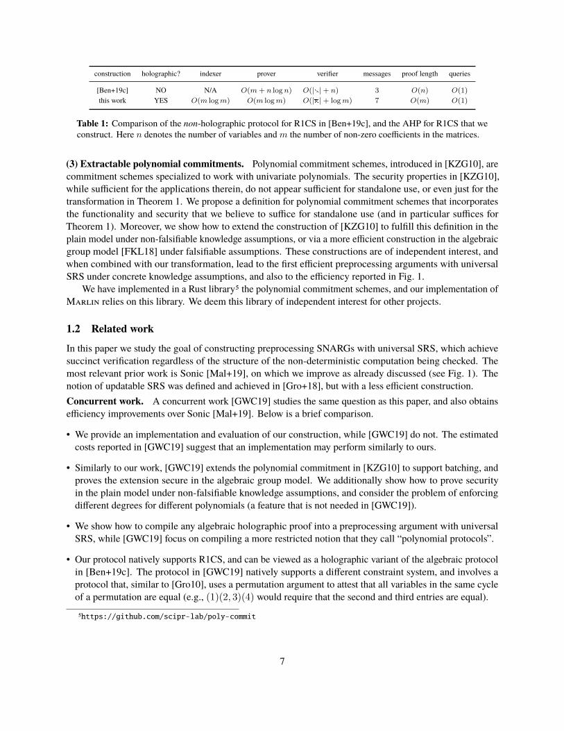
2 Techniques
We discuss the main ideas behind our results. First we describe the two building blocks used in Theorem 1:AHPs and polynomial commitment schemes (described in Sections 2.1 and 2.2 respectively). We describehow to combine these to obtain preprocessing arguments with universal SRS in Section 2.3. Next, we discussconstructions for these building blocks: in Section 2.4 we describe our AHP (underlying Theorem 2), and inSection 2.5 we describe our construction of polynomial commitments.
Throughout, instead of considering the usual notion of relations that consist of instance-witness pairs, weconsider indexed relations, which consist of triples (i,x,w) where i is the index, x is the instance, and w isthe witness. This is because i represents the part of the verifier input that is preprocessed in the offline phase(e.g., the circuit description) and x represents the part of the verifier input that comes in the online phase (e.g.,a partial assignment to the circuit’s input wires). The indexed language corresponding to an indexed relationR, denoted L(R), is the set of pairs (i,x) for which there exists a witness w such that (i,x,w) ∈ R.
2.1 Building block: algebraic holographic proofs
Interactive oracle proofs (IOPs) [BCS16; RRR16] are multi-round protocols where in each round the verifiersends a challenge and the prover sends an oracle (which the verifier can query). IOPs combine featuresof interactive proofs [Bab85; GMR89] and probabilistically checkable proofs [Bab+91; AS98; Aro+98].Algebraic holographic proofs (AHPs) modify the notion of an IOP in two ways.
• Holographic: the verifier does not receive its input explicitly but, rather, has oracle access to a prescribedencoding of it. This potentially enables the verifier to run in time that is much faster than the time to readits input in full. (Our constructions will achieve this fast verification.)
• Algebraic: the honest prover must produce oracles that are low-degree polynomials (this restricts thecompleteness property), and all malicious provers must produce oracles that are low-degree polynomials (thisrelaxes the soundness property). The encoded input to the verifier must also be a low-degree polynomial.
Since in this paper we only work with univariate polynomials, the definitions that we give focus on this casebut they can be modified in a straightforward way to be more general.
Informally, a (public-coin) AHP over a field F for an indexed relation R is specified by an indexer I,prover P, and verifier V that work as follows.
• Offline phase. The indexer I receives as input the index i to be preprocessed, and outputs one or moreunivariate polynomials over F encoding i.
• Online phase. For some instance x and witness w, the prover P receives (i,x,w) and the verifier Vreceives x; P and V interact over some (in this paper, constant) number of rounds, where in each roundV sends a challenge and P sends one or more polynomials; after the interaction, V(x) probabilisticallyqueries the polynomials output by the indexer and the polynomials output by the prover, and then acceptsor rejects. Crucially, V does not receive i as input, but instead queries the polynomials output by I thatencode i. This enables the construction of verifiers V that run in time that is sublinear in |i|.
The completeness property states that for every (i,x,w) ∈ R the probability that P(i,x,w) convincesVI(i)(x) to accept is 1. The soundness property states that for every (i,x) /∈ L(R) and admissible proverP the probability that P convinces VI(i)(x) to accept is at most a given soundness error ε. A prover is“admissible” if the degrees of the polynomials it outputs fit within prescribed degree bounds of the protocol.See Section 4 for details on AHPs, including definitions of proof of knowledge and zero knowledge.
10

Remark 2.1 (prior holographic proofs). Various definitions of “holographic proofs” have been studiedin the literature on probabilistic proofs, starting with the seminal work of Babai, Fortnow, Levin, andSzegedy [Bab+91]. Recent examples include the IPs in [GKR15], whose verifier runs in sublinear time whengiven (multivariate low-degree) encodings of the circuit’s wiring predicates and of the circuit’s input; and alsothe IOPs in [RRR16], where encoded provers and encoded inputs play a role in amortizing interactive proofs.
2.2 Building block: polynomial commitments
Informally, a polynomial commitment scheme [KZG10] allows a prover to produce a commitment c to aunivariate polynomial p ∈ F[X], and later “open” p(X) at any point z ∈ F, producing an evaluation proofπ showing that the opened value is consistent with the polynomial “inside” c at z. Turning this informalgoal into a useful definition requires some care, however, as we explain below. In this paper we propose aset of definitions for polynomial commitment schemes that we believe are useful for standalone use, and inparticular suffice as a building block for our compiler described in Sections 2.3 and 8.
First, we consider constructions with strong efficiency requirements: the commitment c is much smallerthan the polynomial p (e.g., c consists of a constant number of group elements), and the proof π can bevalidated very fast (e.g., in a constant number of cryptographic operations). These requirements not onlyrule out natural constructions,7 but also imply that the usual binding property, which states that an efficientadversary cannot open the same commitment to two different values, does not capture the desired security.Indeed, even if the adversary were to be bound to opening values of some function f : F→ F, it may be thatthe function f is consistent with a polynomial whose degree is higher than what was claimed. This meansthat a security definition needs to incorporate guarantees about the degree of the committed function.8
Second, in many applications of polynomial commitments, an adversary produces multiple commitmentsto polynomials within a round of interaction and across rounds of interaction. After this interaction, theadversary reveals values of all of these polynomials at one or more locations. This setting motivates anumber of considerations. First, it is desirable to rely on a single set of public parameters for committing tomultiple polynomials, even if the polynomials differ in degree. A construction such as that of [KZG10] can bemodified in a natural way to achieve this is by committing both to the polynomial and its shift to the maximumdegree, similarly to techniques used to bundle multiple low-degree tests into a single one [Ben+19c]. Thismodification needs to be addressed in any proof of security. Second, it would be desirable to batch evaluationproofs across different polynomials for the same location. Again the construction in [KZG10] can supportthis, but one must argue that security still holds in this more general case.
The preceeding considerations require an extension of previous definitions and motivate our re-formulationof the primitive. Informally, a polynomial commitment scheme PC is a tuple of algorithms PC = (Setup,Trim,Commit,Open,Check). The setup algorithm PC.Setup takes as input a security parameter andmaximum supported degree boundD, and outputs a committer and receiver key pair (ck, rk) that contains thedescription of a finite field F. The sender can then invoke PC.Commit with input ck and a list of polynomialsp with respective degree bounds d to generate a set of commitments c. Subsequently, the sender can use
7A natural construction would be to use a standard commitment scheme to commit to each coefficient of p, and then open toa value by revealing all of the committed coefficients. However, this construction is inefficient, because the commitment c andevaluation proof π are “long” (linear in the degree of p). An alternative construction would be to use a Merkle tree on the coefficientsof p. While c now becomes short, the evaluation proof π remains long because the receiver would need to see all coefficients tovalidate a claimed evaluation. Crucially, both constructions enable the receiver to check the degree of the committed polynomial.
8This consideration motivates the strong correctness property in [KZG10], which states that if the adversary knows a polynomialthat leads to the claimed commitment c then this polynomial has bounded degree. This notion, while sufficient for the application in[KZG10], does not seem to suffice for standalone use because there is no a priori guarantee that an adversary that can open values toa commitment knows a polynomial inside the commitment. In some sense, a knowledge assumption is hidden in this hypothesis.
11

PC.Open to produce a proof π that convinces the receiver that the polynomials “inside” c respect the degreebounds d and, moreover, evaluate to the claimed set of values v at a given query set Q that specifies anynumber of evaluation points for each polynomial. The receiver can invoke PC.Check to check this proof.
The scheme PC is required to satisfy extractability and succinctness properties, and also, optionally, ahiding property. We outline these properties below (see Section 6.1 for the details).Extractability. Consider an efficient sender adversary A that can produce a commitment c and degreebound d ≤ D such that, when asked for an evaluation at some point z ∈ F, A can produce a supposedevaluation v and proof π such that PC.Check accepts. Then PC is extractable if for every maximum degreebound D and every sender adversary A who can produce such commitments there exists a correspondingefficient extractor EA that outputs a polynomial p of degree at most d that “explains” c so that p(z) = v.While for simplicity we have described the most basic case here, our definition considers adversaries andextractors who interact over multiple rounds, wherein the adversary may produce multiple commitments ineach round and the extractor is required to output corresponding polynomials on a per-round basis (beforeseeing the query set, proof, or supposed evaluations).
In this work we rely on extractability to prove the security of our compiler (see Section 2.3); we do notknow if weaker security notions studied in prior works, such as evaluation binding, suffice. More generally,we believe that extractability is a useful property that may be required across a range of other applications.Succinctness. Commitment size, proof size, and time to verify an opening are independent of the claimeddegrees for the polynomials. (This ensures that the argument produced by our compiler is succinct.)Hiding. The hiding property of PC states that commitments and proofs of evaluation reveal no informationabout the committed polynomial beyond the publicly stated degree bound and the evaluation itself. Namely,PC is hiding if there exists an efficient simulator that outputs simulated commitments and simulated evaluationproofs that cannot be distinguished from their real counterparts by any malicious distinguisher that onlyknows the degree bound and the evaluation.
Analogously to the case of extractability, we actually consider a more general definition that considerscommitments to multiple polynomials within and across multiple rounds; moreover, the definition considersthe case where some polynomials are designated as not hidden (and thus given to the simulator) because inour application we sometimes prefer to commit to a polynomial in a non-hiding way (for efficiency reasons).
2.3 Compiler: from AHPs to preprocessing arguments with universal SRS
We describe the main ideas behind Theorem 1, which uses polynomial commitment schemes to compileany (public-coin) AHP into a corresponding (public-coin) preprocessing argument with universal SRS. In asubsequent step, the argument can be made non-interactive via the Fiat–Shamir transformation, and therebyobtain a preprocessing SNARG with universal SRS.
The basic intuition of the compiler follows the well-known framework of “commit to oracles and thenopen query answers” pioneered by Kilian [Kil92]. However, the commitment scheme used in our compilerleverages and enforces the algebraic structure of these oracles. While several works in the literature alreadytake advantage of algebraic commitment schemes applied to algebraic oracles, our contribution is to observethat if we apply this framework to a holographic proof then we obtain a preprocessing argument.
Informally, first the argument indexer invokes the AHP indexer to generate polynomials, and thendeterministically commits to these using the polynomial commitment scheme. Subsequently, the argumentprover and argument verifier interact, each respectively simulating the AHP prover and AHP verifier. In eachround, the argument prover sends succinct commitments to the polynomials output by the AHP prover in thatround. After the interaction, the argument verifier declares its queries to the polynomials (of the prover and
12

of the indexer). The argument prover replies with the desired evaluations along with an evaluation proofattesting to their correctness relative to the commitments.
This approach, while intuitive, must be proven secure. In particular, in the proof of soundness, we needto show that if the argument prover convinces the argument verifier with a certain probability, then we canfind an AHP prover that convinces the AHP verifier with similar probability. This step is non-trivial: theAHP prover outputs polynomials, while the argument prover merely outputs succinct commitments and a fewevaluations, which is much less information. In order to deduce the former from the latter requires extraction.This motivates considering polynomial commitment schemes that are extractable, in the sense described inSection 2.2. We do not know whether weaker security properties, such as the evaluation binding propertystudied in some prior works, suffice for proving the compiler secure.
The compiler outlined above is compatible with the properties of argument of knowledge and zeroknowledge. Specifically, we prove that if the AHP is a proof of knowledge then the compiler produces anargument of knowledge; also, if the AHP is (bounded-query) zero knowledge and the polynomial commitmentscheme is hiding then the compiler produces a zero knowledge argument.
See Section 8 for more details on the compiler.
2.4 Construction: an AHP for constraint systems
In prior sections we have described how we can use polynomial commitment schemes to compile AHPsinto corresponding preprocessing SNARGs. In this section we discuss the main ideas behind Theorem 2,which provides an efficient AHP for the indexed relation corresponding to R1CS (see Definition 1). Thepreprocessing zkSNARK that we achieve in this paper (see Fig. 1) is based on this AHP.
Our protocol can be viewed as a “holographic variant” of the non-holographic algebraic proof for R1CSconstructed in [Ben+19c]. Achieving holography involves designing a new sub-protocol that enables theverifier to evaluate low-degree extensions of the coefficient matrices at a random location. While in [Ben+19c]the verifier performed this computation in time poly(|i|) on its own, in our protocol the verifier performs itexponentially faster, in time O(log |i|), by receiving help from the prover and having oracle access to thepolynomials produced by the indexer. We introduce notation and then discuss the protocol.Some notation. Consider an index i = (F, n,m,A,B,C) specifying coefficient matrices, an instancex = x ∈ F∗ specifying a partial assignment to the variables, and a witness w = w ∈ F∗ specifying anassignment to the other variables such that the R1CS equation holds. The R1CS equation holds if and only ifAz Bz = Cz for z := (x,w) ∈ Fn. Below, we let H andK be prescribed subsets of F of sizes n andmrespectively; we also let vH(X) and vK(X) be the vanishing polynomials of these two sets. (The vanishingpolynomial of a set S is the monic polynomial of degree |S| that vanishes on S, i.e.,
∏γ∈S(X − γ).) We
assume that bothH andK are smooth multiplicative subgroups. This allows interpolation/evaluation overH in O(n log n) operations and also makes vH(X) computable in O(log n) operations (and similarly forK). Given an n× n matrixM with rows/columns indexed by elements of H , we denote by M(X,Y ) thelow-degree extension ofM , i.e., the polynomial of individual degree less than n such that M(κ, ι) is the(κ, ι)-th entry ofM for every κ, ι ∈ H .A non-holographic starting point. We sketch a non-holographic protocol for R1CS with linear prooflength and constant query complexity, inspired from [Ben+19c], that forms the starting point of our work. Inthis case the prover receives as input (i,x,w) and the verifier receives as input (i,x). (The verifier reads thenon-encoded index i because we are describing a non-holographic protocol.)
In the first message the prover P sends the univariate polynomial z(X) of degree less than n that agreeswith the variable assignment z on H , and also sends the univariate polynomials zA(X), zB(X), zC(X) of
13

degree less than n that agree with the linear combinations zA := Az, zB := Bz, and zC := Cz on H . Theprover is left to convince the verifier that the following two conditions hold:
(1) Entry-wise product: ∀κ ∈ H , zA(κ)zB(κ)− zC(κ) = 0 .
(2) Linear relation: ∀M ∈ A,B,C , ∀κ ∈ H , zM (κ) =∑ι∈H
M [κ, ι]z(ι) .
(The prover also needs to convince the verifier that z(X) encodes a full assignment z that is consistent withthe partial assignment x, but we for simplicity we ignore this in this informal discussion.)
In order to convince the verifier of the first (entry-wise product) condition, the prover sends thepolynomial h0(X) such that zA(X)zB(X) − zC(X) = h0(X)vH(X). This polynomial equation isequivalent to the first condition (the left-hand side equals zero everywhere on H if and only if it is a multipleof H’s vanishing polynomial). The verifier will check the equation at a random point β ∈ F: it querieszA(X), zB(X), zC(X), h0(X) at β, evaluates vH(X) at β on its own, and checks that zA(β)zB(β)−zC(β) =h0(β)vH(β). The soundness error is the maximum degree over the field size, which is at most 2n/|F|.
In order to convince the verifier of the second (linear relation) condition, the prover expects a randomchallenge α ∈ F from the verifier, and then replies in a second message. For eachM ∈ A,B,C, the proversends polynomials hM (X) and gM (X) such that
r(α,X)zM (X)−rM (α,X)z(X) = hM (X)vH(X)+XgM (X) for rM (Z,X) :=∑κ∈H
r(Z, κ)M(κ,X)
where r(Z,X) is a prescribed polynomial of individual degree less than n such that (r(Z, κ))κ∈H aren linearly independent polynomials. Prior work [Ben+19c] on checking linear relations via univariatesumchecks shows that this polynomial equation is equivalent, up to a soundness error of n/|F| over α, to thesecond condition.9 The verifier will check this polynomial equation at the random point β ∈ F: it queriesz(X), zA(X), zB(X), zC(X), hM (X), gM (X) at β, evaluates vH(X) at β on its own, evaluates r(Z,X) andrM (Z,X) at (α, β) on its own, and checks that r(α, β)zM (β)− rM (α, β)z(β) = hM (β)vH(β) + βgM (β).The additional soundness error is 2n/|F|.
The above is a simple 3-message protocol with soundness error max2n/|F|, 3n/|F| = 3n/|F| forR1CS in the setting where the honest prover and malicious provers send polynomials of prescribed degrees,which the verifier can query at any location. The proof length (sum of all degrees) is linear in n and the querycomplexity is constant.Barrier to holography. The verifier in the above protocol runs in time that is Ω(|i|) = Ω(n+m). Whilethis is inherent in the non-holographic setting (because the verifier must read i), we now discuss how exactlythe verifier’s computation depends on i. We shall later use this understanding to achieve an exponentialimprovement in the verifier’s time when given a suitable encoding of i.
The verifier’s check for the entry-wise product is zA(β)zB(β) − zC(β) = h0(β)vH(β), and can becarried out in O(log n) operations regardless of the coefficient matrices contained in the index i. In otherwords, this check is efficient even in the non-holographic setting. However, the verifier’s check for the linearrelation is r(α, β)zM (β)− rM (α, β)z(β) = hM (β)vH(β) + βgM (β), which has a linear cost. Concretely,evaluating the polynomial rM (Z,X) at (α, β) requires Ω(n+m) operations.
A natural idea, in the holographic setting, to reduce this cost would be to grant the verifier oracle accessto the low-degree extension M forM ∈ A,B,C. This idea has two problems: the verifier still needs Ω(n)
9In particular, we are using the fact from [Ben+19c] that, given a multiplicative subgroup S of F, a polynomial f(X) sums to σover S if and only if f(X) can be written as h(X)vS(X) +Xg(X) + σ/|S| for some h(X) and g(X) with deg(g) < |S| − 1.
14

operations to evaluate rM (Z,X) at (α, β) and, moreover, the size of M is quadratic in n, which means thatthe encoding of the index i is Ω(n2). We cannot afford such an expensive encoding in the offline preprocessingphase. We now describe how we overcome both of these problems, and obtain a holographic protocol.Achieving holography. To overcome the above problems and obtain a holographic protocol, we relyrecursively on the univariate sumcheck protocol. We introduce two additional rounds of interaction, and ineach round the verifier learns that their verification equation holds provided the sumcheck from the next roundholds. The last sumcheck will rely on polynomials output by the indexer, which the verifier knows are correct.
We address the first problem by letting the prover and verifier interact in an additional round, where werely on an additional univariate sumcheck to reduce the problem of evaluating rM (Z,X) at (α, β) to theproblem of evaluating M at (β2, β) for a random β2 ∈ F. Namely, the verifier sends β to the prover, whocomputes
σ2 := rM (α, β) =∑κ∈H
r(α, κ)M(κ, β).
Then the prover replies with σ2 and the polynomials h2(X) and g2(X) such that
r(α,X)M(X,β) = h2(X)vH(X) +Xg2(X) + σ2/n .
Prior techniques on univariate sumcheck [Ben+19c] tell us that this equation is equivalent to the polynomialr(α,X)M(X,β) summing to σ2 on H . Thus the verifier needs to check this equation at a random β2 ∈ F:r(α, β2)M(β2, β) = h2(β2)vH(β2) + β2g2(β2) + σ2/n. The only expensive part of this equation for theverifier is computing the value M(β2, β), which is problematic. Indeed, we have already noted that wecannot afford to simply let the verifier have oracle access to M , because this polynomial has quadratic size (itcontains a quadratic number of terms).
We address this second problem as follows. Let uH(X,Y ) := vH(X)−vH(Y )X−Y be the formal derivative of
the vanishing poynomial vH(X), and note that uH(X,Y ) vanishes on the square H ×H except for on thediagonal, where it takes on the (non-zero) values (uH(a, a))a∈H . Moreover, uH(X,Y ) can be evaluated atany point in F × F in O(log n) operations. Using this polynomial, we can write M as a sum of m termsinstead of n2:
M(X,Y ) :=∑κ∈K
uH(X, ˆrowM (κ))uH(Y, colM (κ))valM (κ) ,
where ˆrowM , colM , valM are the low-degree extensions of the row, column, and value of the non-zero entriesinM according to some canonical order overK.10
This method of representing the low-degree extension ofM suggests an idea: let the verifier have oracleaccess to the polynomials ˆrowM , colM , valM and do yet another univariate sumcheck, but this time over thesetK. The verifier sends β2 to the prover, who computes
σ3 := M(β2, β) =∑κ∈K
uH(β2, ˆrowM (κ))uH(β, colM (κ))valM (κ) .
Then the prover replies with σ3 and the polynomials h3(X) and g3(X) such that
uH(β2, ˆrowM (X))uH(β, colM (X))valM (X) = h3(X)vK(X) +Xg3(X) + σ3/m .
The verifier can then check this equation at a random β3 ∈ F, which only requires O(logm) operations.
10Technicality: val(κ) actually equals the value divided by uH( ˆrowM (κ), ˆrowM (κ))uH(colM (κ), colM (κ)).
15

The above idea almost works, the one problem being that h3(X) has degree Ω(nm) (becausethe left-hand size of the equation has quadratic degree), which is too expensive for our target of aquasilinear-time prover. We avoid this problem by letting the prover run the univariate sumcheckprotocol on the unique low-degree extension f(X) of the function f : K → F defined as f(κ) :=uH(β2, ˆrowM (κ))uH(β, colM (κ))valM (κ). Observe that f(X) has degree less thanm. The verifier checksthat f(X) and uH(β2, ˆrowM (X))uH(β, colM (X))valM (X) agree onK.From sketch to protocol. In the above discussion we have ignored a number of technical aspects, such asproof of knowledge and zero knowledge (which are ultimately needed in the compiler if we want to constructa preprocessing zkSNARK). We have also not discussed time complexities of many algebraic steps, and weomitted discussion of how to batch multiple sumchecks into fewer ones, which brings important savings inargument size. For details, see our detailed construction in Section 5.
2.5 Construction: extractable polynomial commitments
We now sketch how to construct a polynomial commitment scheme that achieves the strong functionality andsecurity requirements of our definition in Section 2.2. Our starting point is the PolyCommitDL constructionof Kate et al. [KZG10], and then describe a sequence of natural and generic transformations that extendthis construction to enable extractability, commitments to multiple polynomials, and the enforcement ofper-polynomial degree bounds. In fact, once we arrive at a scheme that supports extractability for committedpolynomials at a single point (Appendix B), our transformations build on this construction in a black box wayto first support per-polynomial degree bounds (Appendix C), and then query sets that may request multipleevaluation points per polynomial (Appendix D). Indeed, it is sufficient to produce a polynomial commitmentscheme that satisfies the much more simple interface and definitions in Appendix B.1, and apply these blackbox transformations to obtain a polynomial commitment scheme that satisfies the interface of and providesthe properties described in Section 6.1 ultimately needed by our compiler.Starting point: PolyCommitDL. The setup phase samples a cryptographically secure bilinear group(G1,G2,GT , q, G,H, e) and then samples a committer key ck and receiver key rk for a given degree boundD. The committer key consists of group elements encoding powers of a random field element β, namely,ck := G, βG, . . . , βDG ∈ GD+1
1 . The receiver key consists of the group elements rk := (G,H, βH) ∈G1 ×G2
2. Note that the SRS, which consists of the keys ck and rk, is updatable because the coefficients ofgroup elements in the SRS are all monomials (see Remark 7.1).
To commit to a polynomial p ∈ Fq[X], the sender computes c := p(β)G. To subsequently provethat the committed polynomial evaluates to v at a point z, the sender computes a witness polynomialw(X) := (p(X)− p(z))/(X − z), and provides as proof a commitment to w: π := w(β)G. The idea is thatthe witness function w is a polynomial if and only if p(z) = v; otherwise, it is a rational function, and cannotbe committed to using ck.
Finally, to verify a proof of evaluation, the receiver checks that the commitment and proof of evaluationare consistent. That is, it checks that the proof commits to a polynomial of the form (p(X)− p(z))/(X − z)by checking the equality e(c− vG,H) = e(π, βH − zH).Achieving extractability. While the foregoing construction guarantees correctness of evaluations, it doesnot by itself guarantee that a commitment actually “contains” a suitable polynomial of degree at most D. Westudy two methods to address this issue, and thereby achieve extractability. One method is to modify theconstruction to use knowledge commitments [Gro10], and rely on a concrete knowledge assumption. Themain disadvantage of this approach is that each commitment doubles in size. The other method is to moveaway from the plain model, and instead conduct the security analysis in the algebraic group model (AGM)
16

[FKL18]. This latter method is more efficient because each commitment remains a single group element.Committing to multiple polynomials at once. We enable the sender to simultaneously open multiplepolynomials [pi]
ni=1 at the same point z as follows. Before generating a proof of evaluation for [pi]
ni=1, the
sender requests from the receiver a random field element ξ, which he uses to take a random linear combinationof the polynomials: p :=
∑ni=1 ξ
ipi, and generates a proof of evaluation π for this polynomial p.The receiver verifies π by using the fact that the commitments are additively homomorphic. The receiver
takes a linear combination of the commitments and claimed evaluations, obtaining the combined commitmentc =
∑ni=1 ξ
ici and evaluation v =∑n
i=1 ξivi. Finally, it checks the pairing equations for c, π, and v.
Completeness of this check is straightforward, while soundness follows from the fact that if any polynomialdoes not match its evaluation, then the combined polynomial will not match its evaluation with high probability.Enforcing multiple degree bounds. The construction so far enforces a single bound D on the degrees ofall the polynomials pi. To enforce a different degree bound di for each pi, we require the sender to commit notonly to each pi, but also to “shifted polynomials” p′i(X) := XD−dipi(X). The proof of evaluation provesthat, if pi evaluates to vi at z, then p
′i evaluates to z
D−divi.The receiver checks that the commitment for each p′i corresponds to an evaluation zD−divi so that, if z is
sampled from a super-polynomial subset of Fq, the probability that deg(pi) 6= di is negligible. This trick issimilar to the one used in [BS08; Ben+19c] to enforce derive low-degree tests for specific degree bounds.
However, while sound, this approach is inefficient in our setting: the witness polynomial for p′i hasΩ(D) non-zero coefficients (instead of O(di)), and so constructing an evaluation proof for it requires Ω(D)scalar multiplications (instead of O(di)). To work around this, we instead produce a proof that the relatedpolynomial p?i (X) := p′i(X) − pi(z)X
D−di evaluates to 0 at z. As we show in Lemma C.2, the witnesspolynomial for this claim has O(di) non-zero coefficients, and so constructing the evaluation proof can bedone in O(di) scalar multiplications. Completeness is preserved because the receiver can check the correctevaluation of p?i by subtracting pi(z)(β
D−diG) from the commitment to the shifted polynomial p′i, therebyobtaining a commitment to p?i , while security is preserved because p
′i(z) = zD−divi ⇐⇒ p?i (z) = 0.
Evaluating at a query set instead of a single point. To support the case where the polynomials [pi]ni=1 are
evaluated at a set of points Q, the sender proceeds as follows. Say that there are k different points [zi]ki=1 in
Q. The sender partitions the polynomials [pi]ni=1 into different groups such that every polynomial in a group
is to be evaluated at the same point zi. The sender runs PC.Open on each group, and outputs the resulting listof evaluation proofs.Achieving hiding. To additionally achieve hiding, we follow the above blueprint, replacing PolyCommitDLwith the hiding scheme PolyCommitPed described in [KZG10].
17

3 Preliminaries
We denote by [n] the set 1, . . . , n ⊆ N. We use a = [ai]ni=1 as a short-hand for the tuple (a1, . . . , an),
and [ai]ni=1 = [[ai,j ]
mj=1]ni=1 as a short-hand for the tuple (a1,1, . . . , a1,m, . . . , an,1, . . . , an,m); |a| denotes
the number of entries in a. If x is a binary string then |x| denotes its bit length. IfM is a matrix then ‖M‖denotes the number of nonzero entries inM . If S is a finite set then |S| denotes its cardinality and x← Sdenotes that x is an element sampled at random from S. We denote by F a finite field, and whenever F is aninput to an algorithm we implicitly assume that F is represented in a way that allows efficient field arithmetic.Given a finite set S, we denote by FS the set of vectors indexed by elements in S. We denote by F[X] the ringof univariate polynomials over F inX , and by F<d[X] the set of polynomials in F[X] with degree less than d.
We denote by λ ∈ N a security parameter. When we state that n ∈ N for some variable n, we implicitlyassume that n = poly(λ). We denote by negl(λ) an unspecified function that is negligible in λ (namely, afunction that vanishes faster than the inverse of any polynomial in λ). When a function can be expressedin the form 1− negl(λ), we say that it is overwhelming in λ. When we say that A is an efficient adversarywe mean that A is a family Aλλ∈N of non-uniform polynomial-size circuits. If the adversary consists ofmultiple circuit families A1,A2, . . . then we write A = (A1,A2, . . . ).
Given two interactive algorithms A and B, we denote by 〈A(x), B(y)〉(z) the output of B(y, z) wheninteracting with A(x, z). Note that this output could be a random variable. If we use this notation when A orB is a circuit, we mean that we are considering a circuit that implements a suitable next-message function tointeract with the other party of the interaction.
3.1 Indexed relations
An indexed relationR is a set of triples (i,x,w) where i is the index, x is the instance, andw is the witness;the corresponding indexed language L(R) is the set of pairs (i,x) for which there exists a witness w suchthat (i,x,w) ∈ R. For example, the indexed relation of satisfiable boolean circuits consists of triples where iis the description of a boolean circuit, x is a partial assignment to its input wires, and w is an assignment tothe remaining wires that makes the circuit to output 0. Given a size bound N ∈ N, we denote by RN therestriction ofR to triples (i,x,w) with |i| ≤ N.
18
4 Algebraic holographic proofs
We define algebraic holographic proofs (AHPs), the notion of proofs that we use. For simplicity, the formaldefinition below is tailored to univariate polynomials, because our AHP construction is in this setting. Thedefinition can be modified in a straightforward way to consider the general case of multivariate polynomials.
We represent polynomials through the coefficients that define them, as opposed to through their evaluationover a sufficiently large domain (as is typically the case in probabilistic proofs). This definitional choice isdue to the fact that we will consider verifiers that may query the polynomials at any location in the fieldof definition. Moreover, the field of definition itself can be chosen from a given field family, and so wemake the field an additional input to all algorithms; this degree of freedom is necessary when combiningthis component with polynomial commitment schemes (see Section 8). Finally, we consider the setting ofindexed relations (see Section 3.1), where the verifier’s input has two parts, the index and the instance; in thedefinition below, the verifier receives the index encoded and the instance explicitly.
Formally, an algebraic holographic proof (AHP) over a field family F for an indexed relation R isspecified by a tuple
AHP = (k, s, d, I,P,V)
where k, s, d : 0, 1∗ → N are polynomial-time computable functions and I,P,V are three algorithmsknown as the indexer, prover, and verifier. The parameter k specifies the number of interaction rounds, sspecifies the number of polynomials in each round, and d specifies degree bounds on these polynomials.
In the offline phase (“0-th round”), the indexer I receives as input a field F ∈ F and an index i forR, and outputs s(0) polynomials p0,1, . . . , p0,s(0) ∈ F[X] of degrees at most d(|i|, 0, 1), . . . , d(|i|, 0, s(0))respectively. Note that the offline phase does not depend on any particular instance or witness, and merelyconsiders the task of encoding the given index i.
In the online phase, given an instance x and witness w such that (i,x,w) ∈ R, the prover P receives(F, i,x,w) and the verifier V receives (F,x) and oracle access to the polynomials output by I(F, i). Theprover P and the verifier V interact over k = k(|i|) rounds.
For i ∈ [k], in the i-th round of interaction, the verifier V sends a message ρi ∈ F∗ to the prover P; thenthe prover P replies with s(i) oracle polynomials pi,1, . . . , pi,s(i) ∈ F[X]. The verifier may query any of thepolynomials it has received any number of times. A query consists of a location z ∈ F for an oracle pi,j , andits corresponding answer is pi,j(z) ∈ F. After the interaction, the verifier accepts or rejects.
The function d determines which provers to consider for the completeness and soundness properties ofthe proof system. In more detail, we say that a (possibly malicious) prover P is admissible for AHP if, onevery interaction with the verifier V, it holds that for every round i ∈ [k] and oracle index j ∈ [s(i)] we havedeg(pi,j) ≤ d(|i|, i, j). The honest prover P is required to be admissible under this definition.
We say that AHP has perfect completeness and soundness error ε if the following holds.
• Completeness. For every field F ∈ F and index-instance-witness tuple (i,x,w) ∈ R, the probability thatP(F, i,x,w) convinces VI(F,i)(F,x) to accept in the interactive oracle protocol is 1.
• Soundness. For every field F ∈ F , index-instance pair (i,x) /∈ L(R), and admissible prover P, theprobability that P convinces VI(F,i)(F,x) to accept in the interactive oracle protocol is at most ε.
The proof length l is the sum of all degree bounds in the offline and online phases, l(|i|) :=∑k(|i|)i=0
∑s(i)j=1 d(|i|, i, j). The intuition for this definition is that in a probabilistic proof each oracle would
consist of the evaluation of a polynomial over a domain whose size (in field elements) is linearly related to itsdegree bound, so that the resulting proof length would be linearly related to the sum of all degree bounds.
19

The query complexity q is the total number of queries made by the verifier to the polynomials. Thisincludes queries to the polynomials output by the indexer and those sent by the prover.
All AHPs that we construct achieve the stronger property of knowledge soundness (against admissibleprovers), and optionally also zero knowledge. We define both of these properties below.Knowledge soundness. We say thatAHP has knowledge error ε if there exists a probabilistic polynomial-timeextractor E for which the following holds. For every field F ∈ F , index i, instance x, and admissible proverP, the probability that EP(F, i,x, 1l(|i|)) outputs w such that (i,x,w) ∈ R is at least the probability that P
convinces VI(F,i)(F,x) to accept minus ε. Here the notation EP means that the extractor E has black-boxaccess to each of the next-message functions that define the interactive algorithm P. (In particular, theextractor E can “rewind” the prover P.) Note that since E receives the proof length l(|i|) in unary, E hasenough time to receive, and perform efficient computations on, polynomials output by P.Zero knowledge. We say that AHP has (perfect) zero knowledge with query bound b and query checker Cif there exists a probabilistic polynomial-time simulator S such that for every field F ∈ F , index-instance-witness tuple (i,x,w) ∈ R, and (b,C)-query algorithm V the random variables View(P(F, i,x,w), V)
and SV(F, i,x), defined below, are identical. Here, we say that an algorithm is (b,C)-query if it makes atmost b queries to oracles it has access to, and each query individually leads the checker C to output “ok”.
• View(P(F, i,x,w), V) is the view of V, namely, is the random variable (r, a1, . . . , aq) where r is V’srandomness and a1, . . . , aq are the responses to V’s queries determined by the oracles sent by P(F, i,x,w).
• SV(F, i,x) is the output of S(F, i,x) when given straightline access to V (S may interact with V, withoutrewinding, by exchanging messages with V and answering any oracle queries along the way), prependedwith V’s randomness r. Note that r could be of super-polynomial size, so S cannot sample r on V’s behalfand then output it; instead, as in prior work, we restrict S to not see r, and prepend r to S’s output.
A special case of interest. We only consider AHPs that satisfy the following properties.
– Public coins: AHP is public-coin if each verifier message to the prover is a uniformly random string of someprescribed length (or an empty string). Hence the verifier’s randomness is its messages ρ1, . . . , ρk ∈ F∗ andpossibly additional randomness ρk+1 ∈ F∗ used after the interaction. All verifier queries can be postponed,without loss of generality, to a query phase that occurs after the interactive phase with the prover.
– Non-adaptive queries: AHP is non-adaptive if all of the verifier’s query locations are solely determined bythe verifier’s randomness and inputs (the field F and the instance x).
Given these properties, we can view the verifier as two subroutines that execute in the query phase: a queryalgorithm QV that produces query locations based on the verifier’s randomness, and a decision algorithmDV that accepts or rejects based on the answers to the queries (and the verifier’s randomness). In more detail,QV receives as input the field F, the instance x, and randomness ρ1, . . . , ρk, ρk+1, and outputs a query set Qconsisting of tuples ((i, j), z) to be interpreted as “query pi,j at z ∈ F”; and DV receives as input the field F,the instance x, answers (v((i,j),z))((i,j),z)∈Q, and randomness ρ1, . . . , ρk, ρk+1, and outputs the decision bit.
While the above properties are not strictly necessary for the compiler that we describe in Section 8,all “natural” protocols that we are aware of (including those that we construct in this paper) satisfy theseproperties, and so we restrict our attention to public-coin non-adaptive protocols for simplicity.
20

5 AHP for constraint systems
We construct an AHP for rank-1 constraint satisfiability (R1CS) that has linear proof length and constantquery complexity. Below we define the indexed relation that represents this problem, and then state our result.
Definition 5.1 (R1CS indexed relation). The indexed relationRR1CS is the set of all triples
(i,x,w) =((F, H,K,A,B,C), x, w
)where F is a finite field, H and K are subsets of F, A,B,C are H × H matrices over F with |K| ≥max‖A‖, ‖B‖, ‖C‖, and z := (x,w) is a vector in FH such that Az Bz = Cz.
Theorem 5.2. There exists an AHP for the indexed relationRR1CS that is a zero knowledge proof of knowledgewith the following features. The indexer uses O(|K| log |K|) field operations and outputs O(|K|) fieldelements. The prover and verifier exchange 7 messages. To achieve zero knowledge against b queries (with aquery checker C that rejects queries in H), the prover uses O((|K|+ b) log(|K|+ b)) field operations andoutputs a total of O(|H|+ b) field elements. The verifier makes O(1) queries to the encoded index and to theprover’s messages, has soundness error O((|K|+ b)/|F|), and uses O(|x|+ log |K|) field operations.
Remark 5.3 (restrictions on domains). Our protocol uses the univariate sumcheck of [Ben+19c] as a subroutine,and in particular inherits the requirement that the domains H and K must be additive or multiplicativesubgroups of the field F. For simplicity, in our descriptions we use multiplicative subgroups because we usethis case in our implementation; the case of additive subgroups involves only minor modifications. Moreover,the arithmetic complexities for the indexer and prover stated in Theorem 5.2 assume that the domainsH andK are “FFT-friendly” (e.g., they have smooth sizes); this is not a requirement, since in general the arithmeticcomplexities will be that of an FFT over the domains H and K. Note that we can assume without loss ofgenerality that |H| = O(|K|), for otherwise (if |K| < |H|/3) then are empty rows or columns across thematrices that we can drop and reduce their size. Finally, we assume that |H| ≤ |F|/2.
This section is organized as follows: in Section 5.1 we introduce algebraic notations and facts used inthis section; in Section 5.2 we describe an AHP for checking linear relations; and in Section 5.3 we build onthis latter to obtain an AHP for R1CS. Throughout we assume that H andK come equipped with bijectionsφ
H: H → [|H|] and φ
K: K → [|K|] that are computable in linear time. Moreover, we define the two sets
H[≤ k] := κ ∈ H : 1 ≤ φH
(κ) ≤ k and H[> k] := κ ∈ H : φH
(κ) > k to denote the first k elementsin H and the remaining elements, respectively. We can then write that x ∈ FH[≤|x|] and w ∈ FH[>|x|].
5.1 Algebraic preliminaries
Polynomial encodings. For a finite field F, subset S ⊆ F, and function f : S → F we denote by f the(unique) univariate polynomial over F with degree less than |S| such that f(a) = f(a) for every a ∈ S. Wesometimes abuse notation and write f to denote some polynomial that agrees with f on S, which need notequal the (unique) such polynomial of smallest degree.Vanishing polynomials. For a finite field F and subset S ⊆ F, we denote by vS the unique non-zero monicpolynomial of degree at most |S| that is zero everywhere on S; vS is called the vanishing polynomial of S. IfS is an additive or multiplicative coset in F then vS can be evaluated in polylog(|S|) field operations. Forexample, if S is a multiplicative subgroup of F then vS(X) = X |S| − 1 and, more generally, if S is a ξ-cosetof a multiplicative subgroup S0 (namely, S = ξS0) then vS(X) = ξ|S|vS0
(X/ξ) = X |S| − ξ|S|; in eithercase, vS can be evaluated in O(log |S|) field operations.
21

Derivative of vanishing polynomials. We rely on various properties of a bivariate polynomial uS introducedin [Ben+19b]. For a finite field F and subset S ⊆ F, we define
uS(X,Y ) :=vS(X)− vS(Y )
X − Y,
which is a polynomial of individual degree |S| − 1 becauseX − Y dividesXi − Y i for any positive integer i.Note that uS(X,X) is the formal derivative of the vanishing polynomial vS(X). The bivariate polynomialuS(X,Y ) satisfies two useful algebraic properties. First, the univariate polynomials (uS(X, a))a∈S arelinearly independent, and uS(X,Y ) is their (unique) low-degree extension. Second, uS(X,Y ) vanishes onthe square S × S except for on the diagonal, where it takes on the (non-zero) values (uS(a, a))a∈S .
If S is an additive or multiplicative coset in F, uS(X,Y ) can be evaluated at any (α, β) ∈ F2 inpolylog(|S|) field operations because in this case both vS (and its derivative) can be evaluated in polylog(|S|)field operations. For example, if S is a multiplicative subgroup then uS(X,Y ) = (X |S| − Y |S|)/(X − Y )
and uS(X,X) = |S|X |S|−1, so both can be evaluated in O(log |S|) field operations.Univariate sumcheck for subgroups. Prior work [Ben+19c] shows that, given a multiplicative subgroup Sof F, a polynomial f(X) sums to σ over S if and only if f(X) can be written as h(X)vS(X)+Xg(X)+σ/|S|for some h(X) and g(X) with deg(g) < |S| − 1. This can be viewed as a univariate sumcheck protocol, andwe shall rely on it throughout this section.
5.2 AHP for the lincheck problem
The lincheck problem for univariate polynomials considers the task of deciding whether two polynomialsencode vectors that are linearly related in a prescribed way. In more detail, the problem is parametrized by afield F, two subsets H and K of F, and a matrixM ∈ FH×H with |K| ≥ ‖M‖ > 0. Given oracle accessto two low-degree polynomials f1, f2 ∈ F<d[X], the problem asks to decide whether for every a ∈ H itholds that f1(a) =
∑b∈HMa,b · f2(b), by asking a small number of queries to f1 and f2. The matrixM thus
prescribes the linear relations that relate the values of f1 and f2 on H .Ben-Sasson et al. [Ben+19c] solve this problem by reducing the lincheck problem to a sumcheck problem,
and then reducing the sumcheck problem to low-degree testing (of univariate polynomials). In particular,this prior work achieves a 2-message algebraic non-holographic protocol that solves the lincheck problemwith linear proof length and constant query complexity. In this section we show how to achieve a 6-messagealgebraic holographic protocol, again with linear proof length and constant query complexity. In Section 5.2.1we describe the indexer algorithm, in Section 5.2.2 we describe the prover and verifier algorithms, and inSection 5.2.3 we analyze the protocol. Fig. 4 summarizes the protocol.
5.2.1 Offline phase: encoding the linear relation
The indexer I for the lincheck problem receives as input a field F, two subsetsH andK of F, and a matrixM ∈ FH×H with |K| ≥ ‖M‖. The non-zero entries ofM are assumed to be presented in some canonicalorder (e.g., row-wise or column-wise). The output of I is three univariate polynomials ˆrow, col, val over F ofdegree less than |K| such that the following polynomial is a low-degree extension ofM :
M(X,Y ) :=∑κ∈K
uH(X, ˆrow(κ))uH(Y, col(κ))val(κ) . (1)
22

The three three aforementioned polynomials are the (unique) low-degree extensions of the three functionsrow, col, val : K → F that respectively represent the row index, column index, and value of the non-zeroentries of the matrixM . In more detail, for every κ ∈ K with 1 ≤ φ
K(κ) ≤ ‖M‖:
• row(κ) := φ−1H
(tκ) where tκ is the row index of the φK
(κ)-th nonzero entry inM ;• col(κ) := φ−1
H(tκ) where tκ is the column index of the φ
K(κ)-th nonzero entry inM ;
• val(κ) is the value of the φK
(κ)-th nonzero entry inM , divided by uH(row(κ), row(κ))uH(col(κ), col(κ)).
Also, val(κ) returns the element 0 for every κ ∈ K with φK
(κ) > ‖M‖, while row(κ) and col(κ) return anarbitrary element in H for such κ. The evaluation tables of these functions can be found in O(|K| log |H|)operations, from which interpolation yields the desired polynomials in O(|K| log |K|) operations.
Recall from Section 5.1 that the bivariate polynomial uH(X,Y ) vanishes on the squareH ×H except foron the diagonal, where it takes on the (non-zero) values (uH(a, a))a∈H . By construction of the polynomialsˆrow, col, val, the polynomial M(X,Y ) agrees with the matrixM everywhere on the domain H ×H . The
individual degree of M(X,Y ) is less than |H|. Thus, M is the unique low-degree extension ofM .We rewrite the polynomial M(X,Y ) in a form that will be useful later:
Claim 5.4.M(X,Y ) =
∑κ∈K
vH(X)
(X − ˆrow(κ))· vH(Y )
(Y − col(κ))· val(κ) . (2)
Proof. Note that vH( ˆrow(κ)) = vH(col(κ)) = 0 for every κ ∈ K because ˆrow(X) and col(X) mapK toHand vH vanishes on H . Therefore:
M(X,Y ) =∑κ∈K
uH(X, ˆrow(κ)) · uH(Y, col(κ)) · val(κ)
=∑κ∈K
vH(X)− vH( ˆrow(κ))
X − ˆrow(κ)· vH(Y )− vH(col(κ))
Y − col(κ)· val(κ)
=∑κ∈K
vH(X)
(X − ˆrow(κ))· vH(Y )
(Y − col(κ))· val(κ) .
5.2.2 Online phase: proving and verifying the linear relation
The prover P for the lincheck problem receives as input a field F, two subsets H and K of F, a matrixM ∈ FH×H with |K| ≥ ‖M‖, and two polynomials f1, f2 ∈ F<d[X]. The verifier V for the lincheckproblem receives as input the field F and two subsets H and K of F; V also has oracle access to thepolynomials ˆrow, col, val output by the indexer I invoked on appropriate inputs.
The protocol begins with a reduction from a lincheck problem to a sumcheck problem: V samples arandom element α ∈ F and sends it to P. Indeed, letting r(X,Y ) denote the polynomial uH(X,Y ), P is leftto convince V that the following univariate polynomial sums to 0 on H:
q1(X) := r(α,X)f1(X)− rM (α,X)f2(X) where rM (X,Y ) :=∑κ∈H
r(X,κ)M(κ, Y ) . (3)
23

We rely on the univariate sumcheck protocol for this step: P sends to V the polynomials g1(X)and h1(X) such that q1(X) = h1(X)vH(X) + Xg1(X). In order to check this polynomial identity, Vsamples a random element β1 ∈ F with the intention of checking the identity at X := β1. For theright-hand side, V queries g1 and h1 at β1, and then evaluates h1(β1)vH(β1) + β1g1(β1) in O(log |H|)operations. For the left-hand side, V queries f1 and f2 at β1 and then needs to ask help from P toevaluate r(α, β1)f1(β1)− rM (α, β1)f2(β1). The reason is that while r(α, β1) is easy to evaluate (it requiresO(log |H|) operations), rM (α, β1) =
∑κ∈H r(α, κ)M(κ, β1) in general requires Ω(|H||K|) operations.
We thus rely on the univariate sumcheck protocol again. We define
q2(X) := r(α,X)M(X,β1) (4)
V sends β1 to P, and then P replies with the sum σ2 :=∑
κ∈H r(α, κ)M(κ, β1) and the polynomialsg2(X) and h2(X) such that q2(X) = h2(X)vH(X) +Xg2(X) + σ2/|H|. In order to check this polynomialidentity, V samples a random element β2 ∈ F with the intention of checking the identity at X := β2. Forthe right-hand side, V queries g2 and h2 at β2, and then evaluates h2(β2)vH(β2) + β2g2(β2) + σ2/|H| inO(log |H|) operations. To evaluate the left-hand side, however, V needs to ask help from P. The reasonis that while r(α, β2) is easy to evaluate (it requires O(log |H|) operations), M(β2, β1) in general requiresΩ(|K|) operations.
We thus rely on the univariate sumcheck protocol (yet) again: V sends β2 to P, and then P replies withthe value σ3 := M(β2, β1), which the verifier must check. Note though that we cannot use the sumcheckprotocol directly to compute the sum obtained from Eq. (1):
M(β2, β1) =∑κ∈K
uH(β2, ˆrow(κ))uH(β1, col(κ))val(κ) .
The reason is because the degree of the above addend, if we replace κ with an indeterminate, is Ω(|H||K|),which means that the degree of the polynomial h3 sent as part of a sumcheck protocol also has degreeΩ(|H||K|), which is not within our budget of an AHP with proof length O(|H|+ |K|). Instead, we makethe minor modification that in the earlier rounds β1 and β2 are sampled from F \H instead of F, and we willleverage the sumcheck protocol to verify the equivalent (well defined) expression from Eq. (2):
M(β2, β1) =∑κ∈K
vH(β2)vH(β1)val(κ)
(β2 − ˆrow(κ))(β1 − col(κ)).
This may appear to be an odd choice, because if we replace κ with an indeterminate in the sum above, weobtain a rational function that is (in general) not a polynomial, and so does not immediately fit the sumcheckprotocol. Nevertheless, we are still able to use the sumcheck protocol with it, as we now explain.
Define f3(X) to be the (unique) polynomial of degree less than |K| such that
∀κ ∈ K , f3(κ) =vH(β2)vH(β1)val(κ)
(β2 − ˆrow(κ))(β1 − col(κ)). (5)
The prover computes the polynomials g3(X) and h3(X) such that
f3(X) = Xg3(X) + σ3/|K| ,vH(β2)vH(β1)val(X)− (β2 − ˆrow(X))(β1 − col(X))f3(X) = h3(X)vK(X) .
24

The first equation demonstrates that f3 sums to σ3 over K, and the second equation demonstrates thatf3 agrees with the correct addends overK. These two equations can be combined in a single equation thatinvolves only g3(X) and h3(X):
vH(β2)vH(β1)val(X)− (β2 − ˆrow(X))(β1 − col(X))(Xg3(X) + σ3/|K|) = h3(X)vK(X) .
The prover thus only sends the two polynomials g3(X) and h3(X). In order to check this polynomialidentity, V samples a random element β3 ∈ F with the intention of checking the identity at X := β3. ThenV queries g3, h3, ˆrow, col, val at β3, and then evaluates vH(β2)vH(β1)val(β3) − (β2 − ˆrow(β3))(β1 −col(β3))(β3g3(β3) + σ3/|K|) = h3(β3)vK(β3) in O(log |K|) operations.
If this third test passes then V can use the value σ3 in place of M(β2, β1) to finish the second test. If thislatter passes, V can in turn use the value σ2 in place of rM (α, β1) to finish the first test.
5.2.3 Analysis
Soundness. We argue that the soundness error is at most
|H|+ 3|K||F|
+d+ 3|H||F \H|
.
There are four ways in which the verifier could still accept if the lincheck statement is false: if the randomizedreduction to the first sumcheck produces a polynomial that sums to zero; or if any one of the three sumchecksaccepts despite the claimed sum being incorrect. The probability that the randomized reduction to sumcheckfails is at most the individual degree in X of r(X,Y ) divided by |F|, which is less than |H|/|F|. Theprobability that any one of the sumchecks fail to detect an incorrectly declared sum is at most the maximumdegree of the polynomial equation tested in the respective sumcheck divided by the size from which thetest element is sampled. The innermost sumcheck has maximum degree less than 3|K|, the intermediatesumcheck has maximum degree less than 2|H|, and the outermost sumcheck has maximum degree less than|H|+ d. These errors add up to the soundness error claimed above.Efficiency. The protocol consists of 6 messages, with the verifier moving first. The verifier makes a constantnumber of queries, evaluates vH and vK at a constant number of locations, and then performs a constantnumber of field operations. In particular, the arithmetic complexity of the verifier is O(log |H|+ log |K|).The prover sends a constant number of polynomials with degrees linearly related to d (the bound on the degreesof f1 and f2), |H|, and |K|. We now argue that prover time is O((|H|+ d) log(|H|+ d) + |K| log |K|). Inthe first round, the prover sends the coefficients of the polynomials g1(X) and h1(X), which can be found intime O(|K|+ (|H|+ d) log(|H|+ d)), as we argue in Lemma 5.5. In the second round, the prover sends thefield element σ2 and the polynomials g2(X) and h2(X), which can be found in time O(|K|+ |H| log |H|),as we argue in Lemma 5.6. In the third round, the prover sends the field element σ3 and the polynomialsg3(X) and h3(X), which can be found in time O(|K| log |K|), as we argue in Lemma 5.7.
Lemma 5.5 (first round). The coefficients of the polynomials g1(X) and h1(X) can be found in O(|K| +(|H|+ d) log(|H|+ d)) field operations, when given coefficients of the polynomials f1(X) and f2(X), thesubsets H andK, and the matrixM (in sparse form).
Proof. It suffices to find the coefficients of the polynomial q1(X) from Eq. (3), which has degree at most|H|+ d− 2, because the polynomials g1(X) and h1(X) can be found via polynomial long division of q1(X)by vH in time O((|H|+ d) log |H|). In turn, q1(X) can be computed from the coefficients of f1(X), f2(X),
25

r(α,X), and rM (α,X) in timeO((|H|+d) log(|H|+d)) via fast polynomial multiplication and polynomialaddition. The first two are given to us in coefficient form; to find the coefficients of the latter two polynomials,we can evaluate each of them over H and then interpolate.
The values of r(α,X) on H can be obtained in O(|H| log |H|) operations via direct computation offormulas described in Section 5.1. The problem is now reduced to finding the values of rM (α,X) on H —this is the “hard part” that motivates the present proof.
Observe that, by definition of rM (see Eq. (3)) and M (see Eq. (1)), the following holds:
rM (α,X) =∑κ1∈H
r(α, κ1)∑κ2∈K
uH(κ1, ˆrow(κ2))uH(X, col(κ2))val(κ2)
=∑κ2∈K
uH(X, col(κ2))val(κ2)∑κ1∈H
r(α, κ1)uH(κ1, ˆrow(κ2))
=∑κ2∈K
uH(X, col(κ2))val(κ2)r(α, ˆrow(κ2))uH( ˆrow(κ2), ˆrow(κ2)) .
The last equality uses the fact that, for every κ2 ∈ K, the summation∑
κ1∈H r(α, κ1)uH(κ1, ˆrow(κ2))collapses to a single term corresponding to κ1 = ˆrow(κ2); the other terms, which correspond to κ1 6= ˆrow(κ2),are zero due to the fact that the polynomial uH vanishes on the square H ×H except for on its diagonal.
Next, again using the fact that uH vanishes on the square H ×H except for on its diagonal, we note thatfor every κ1 ∈ H
rM (α, κ1) =∑
κ2∈K s.t. col(κ2)=κ1
uH(κ1, col(κ2))val(κ2) · r(α, ˆrow(κ2))uH( ˆrow(κ2), ˆrow(κ2)) .
In other words, as κ1 ranges over H , each element of the sum in rM (α, κ1) contributes a nonzero valueprecisely when κ1 equals a particular element of H , namely, when κ1 = col(κ2). Also, since κ2 ranges onlyinK, ˆrow(κ2) = row(κ2), col(κ2) = col(κ2), and val(κ2) = val(κ2) are just the row index, column index,and value of the κ2-th entry ofM (or zero).
This immediately leads to the following strategy to finding the values of rM (α,X) on H . Ini-tialize for each κ1 ∈ H a variable for rM (α, κ1) that is initially set to 0. Then, for each κ2 ∈ K,compute the term uH(col(κ2), col(κ2))val(κ2)r(α, row(κ2))uH(row(κ2), row(κ2)) and add it to the vari-able for rM (α, col(κ2)). Since the values (uH(κ1, κ1))κ1∈H and (r(α, κ1))κ1∈H can be precomputed inO(|H| log |H|) operations, the foregoing strategy can be carried out inO(|K|+ |H| log |H|) operations.
Lemma 5.6 (second round). The field element σ2 and the coefficients of the polynomials g2(X) and h2(X)can be found in O(|K|+ |H| log |H|) field operations, when given the subsets H andK and the matrixM(in sparse form).
Proof. It suffices to find the coefficients of the polynomial q2(X) from Eq. (4), which has degree at most2|H| − 2, because the polynomials g2(X) and h2(X) can be found via polynomial long division of q2(X) byvH in time O(|H| log |H|), and the sum σ2 can be found by evaluating q2(X) overH in time O(|H| log |H|)and summing in time O(|H|). In turn, q2(X) can be computed from the coefficients of r(α,X) and ofM(X,β1) in time O(|H| log |H|) using fast polynomial multiplication. To find the coefficients of these twopolynomials, we can evaluate each of them over H and then interpolate. The values of r(α,X) on H can beobtained in O(|H| log |H|) operations. We now need to find the values of M(X,β1) on H .
Recall thatM(X,β1) =
∑κ∈K
uH(X, ˆrow(κ))uH(β1, col(κ))val(κ) .
26

Using the fact that uH vanishes on the square H ×H except for the diagonal, we note that for everyκ1 ∈ H
M(κ1, β1) =∑
κ2∈K s.t. ˆrow(κ2)=κ1
uH(κ1, ˆrow(κ2))uH(β1, col(κ2))val(κ2) .
Thus, to find the values of of M(X,β1) onH , we initialize for each κ1 ∈ H a variable for M(κ1, β1) that isinitially set to 0. Then, for each κ2 ∈ K, we compute the term uH( ˆrow(κ2), ˆrow(κ2))uH(β1, col(κ2))val(κ2)and add it to the variable for M( ˆrow(κ2), β1). Since the values (uH(κ, κ))κ∈H and (uH(β1, κ))κ∈H can beprecomputed in O(|H| log |H|) operations, the foregoing strategy can be carried out in O(|K|+ |H| log |H|)operations.
Lemma 5.7 (third round). The field element σ3 and the coefficients of the polynomials g3(X) and h3(X) canbe found in O(|K| log |K|) field operations, when given the subsets H andK and the matrixM (in sparseform).
Proof. First, we find the coefficients of the polynomial f3(X) from Eq. (5), which has degree at most |K| − 1.We traverse the matrixM to find the values of ˆrow(κ) = row(κ), col(κ) = col(κ), and val(κ) = val(κ), forevery κ ∈ K. Then, for each κ ∈ K, we calculate f3(κ) = vH(β2)vH(β1)val(κ)
(β2− ˆrow(κ))(β1−col(κ)), and interpolate those |K|
values, in time O(|K| log |K|). Those values can also be summed, in time O(|K|), to obtain σ3. Then g3(X)can be found easily, by subtracting σ3/|K| from f3(X) and dividing by X .
Next, the prover interpolates the values fromM to find the three polynomials ˆrow, col, and val. Using fastpolynomial multiplication, the prover calculates vH(β2)vH(β1)val(X)−(β2− ˆrow(X))(β1− col(X))f3(X),and divides this polynomial by vK(X) to find h3(X). This too can be done in time O(|K| log |K|).
5.3 AHP for R1CS
We prove Theorem 5.2. In Section 5.3.1 we describe the indexer algorithm, in Section 5.3.2 we describe theprover and verifier algorithms, and in Section 5.3.3 we analyze the protocol. Fig. 5 summarizes the protocol.
The AHP for R1CS directly builds on the AHP for the lincheck problem, analogously to how in [Ben+19c]the non-holographic protocol for R1CS builds on the non-holographic lincheck protocol. The three lincheckproblems associated to the three matrices in the index are bundled together via random coefficients, whilethe entry-wise product is checked with a polynomial identity. Zero knowledge is achieved via boundedindependence and random masks [Ben+16; Ben+19c]. Consistency with the instance is achieved by havingthe verifier combine a low-degree extension of the instance and the low-degree extension of the (alleged)witness sent by the prover, in order to create a low-degree extension of the full assignment.
5.3.1 Offline phase: encoding the constraint system
The indexer I for R1CS receives as input a field F, two subsets H and K of F, and three matricesA,B,C ∈ FH×H with |K| ≥ max‖A‖, ‖B‖, ‖C‖. The non-zero entries of A,B,C are assumed to bepresented in some common canonical order. The output of I consists of the output of the lincheck indexerseparately invoked on A,B,C. This produces nine univariate polynomials ˆrowM , colM , valMM∈A,B,Cover F of degree less than |K| that can be used to compute the low-degree extensions of A,B,C.
27

5.3.2 Online phase: proving and verifying satisfiability
The prover P for R1CS receives as input a field F, two subsetsH andK of F, three matricesA,B,C ∈ FH×H
with |K| ≥ max‖A‖, ‖B‖, ‖C‖, input x ∈ FH[≤|x|], and witness w ∈ FH[>|x|]. The verifier V for R1CSreceives as input the field F, two subsets H andK of F, and input x ∈ FH[≤|x|]; V also has oracle access tothe polynomials ˆrowM , colM , valMM∈A,B,C output by the indexer I invoked on appropriate inputs.
The protocol begins with the prover sending randomized encodings for (a certain shift of) the assignmentand its linear combinations. Define x(X) to be the polynomial of degree less than |x| that agrees with theinstance x in H[≤ |x|]. Define the shifted witness w : H[> |x|]→ F according to the equation
∀ γ , w(γ) :=w(γ)− x(γ)
vH[≤|x|](γ).
The prover P sends to V a random w(X) ∈ F<|w|+b[X] that agrees with w on H[> |x|]; P also setsz := (x,w) ∈ FH to be the full assignment, computes the three linear combinations zA := Az, zB := Bz,and zC := Cz, and sends to V random zA(X), zB(X), zC(X) ∈ F<|H|+b[X] that agree with zA, zB, zC onH . Note that the values of up to b locations in each of w(X), zA(X), zB(X), zC(X) reveal no informationabout the witness w, provided the locations are in F \H . Note also that z(X) := w(X)vH[≤|x|](X) + x(X)agrees with z on H; moreover, V can evaluate z(X) at any location γ with O(|x|) operations by querying wat γ and computing the expression w(γ)vH[≤|x|](γ) + x(γ) by using x.
The rest of the protocol is for P to convince V that zA zB = zC and also that zA, zB, zC are obtainedas linear combinations from z.
In the same message as above, P also sends to V the polynomial h0(X) such that zA(X)zB(X) −zC(X) = h0(X)vH(X). In addition, P sends to V a (fully) random s(X) ∈ F<2|H|+b−1[X] and its sumσ1 :=
∑κ∈H s(κ) over H . This random polynomial will be used as a “mask” to make the univariate
sumcheck zero knowledge.Next, V samples random elements α, ηA, ηB, ηC ∈ F and sends them to P. The element α is used to
reduce lincheck problems to sumcheck, while the elements ηA, ηB, ηC are used to bundle the three sumcheckproblems into one. Indeed, P is left to convince V that the following univariate polynomial sums to σ1 onH:
q1(X) := s(X) + r(α,X)
∑M∈A,B,C
ηM ˆzM (X)
− ∑M∈A,B,C
ηMrM (α,X)
z(X) (6)
where rM (X,Y ) :=∑
κ∈H r(X,κ)M(κ, Y ).We now rely on the univariate sumcheck protocol: P sends to V the polynomials g1(X) and h1(X) such
that q1(X) = h1(X)vH(X) + Xg1(X). In order to check this polynomial identity, V samples a randomelement β1 ∈ F \H with the intention of checking the identity atX := β1. For the right-hand side, V queriesg1 and h1 at β1 and then evaluates h1(β1)vH(β1) + β1g1(β1) in O(log |H|) operations. For the left-handside, V queries s, zA, zB, zC , w at β1 and then needs to ask help from P to evaluate q1(β1). The reason is thatthe term ηArA(α, β1) + ηBrB(α, β1) + ηCrC(α, β1) in general requires Ω(|H||K|) operations to compute.
Observe that
ηArA(α, β1) + ηBrB(α, β1) + ηCrC(α, β1)
= ηA∑κ∈H
r(α, κ)A(κ, β1) + ηB∑κ∈H
r(α, κ)B(κ, β1) + ηC∑κ∈H
r(α, κ)C(κ, β1)
28

=∑κ∈H
r(α, κ)(ηAA(κ, β1) + ηBB(κ, β1) + ηCC(κ, β1)) .
We define the polynomial
q2(X) := r(α,X)(ηAA(X,β1) + ηBB(X,β1) + ηCC(X,β1)) (7)
and rely on the univariate sumcheck protocol again: V sends β1 to P, and then P replies with the sum σ2 :=∑κ∈H q2(κ) and the polynomials g2(X) and h2(X) such that q2(X) = h2(X)vH(X) +Xg2(X) + σ2/|H|.
In order to check this polynomial identity, V samples a random element β2 ∈ F \H with the intention ofchecking the identity at X := β2. (Excluding H is needed later in the protocol, as discussed below.) Forthe right-hand side, V queries g2 and h2 at β2, and then evaluates h2(β2)vH(β2) + β2g2(β2) + σ2/|H| inO(log |H|) operations. To evaluate the left-hand side, however, V needs to ask help from P. The reason isthat while r(α, β2) is easy to evaluate (it requires O(log |H|) operations), each term M(β2, β1) in generalrequires Ω(|K|) operations.
We thus rely on the univariate sumcheck protocol (yet) again: V sends β2 to P, and then P replies withthe value σ3 := ηAA(β2, β1) + ηBB(β2, β1) + ηCC(β2, β1), which the verifier much check. Observe that
ηAA(β2, β1) + ηBB(β2, β1) + ηCC(β2, β1) =∑κ∈K
∑M∈A,B,C
ηMvH(β2)vH(β1)valM (κ)
(β2 − ˆrowM (κ))(β1 − colM (κ)).
Define f3(X) to be the (unique) polynomial of degree less than |K| such that
∀κ ∈ K , f3(κ) =∑
M∈A,B,C
ηMvH(β2)vH(β1)valM (κ)
(β2 − ˆrowM (κ))(β1 − colM (κ)). (8)
The prover computes the polynomials g3(X) and h3(X) such that
f3(X) = Xg3(X) + σ3/|K| and a(X)− b(X)f3(X) = h3(X)vK(X)
where
a(X) :=∑
M∈A,B,C
ηMvH(β2)vH(β1)valM (X)∏
N∈A,B,C\M
(β2 − ˆrowN (X))(β1 − colN (X)) ,
b(X) :=∏
M∈A,B,C
(β2 − ˆrowM (X))(β1 − colM (X)) .
The first equation demonstrates that f3 sums to σ3 over K, and the second equation demonstrates that f3
agrees with the correct addends over K. These two equations can be combined in a single equation thatinvolves only g3(X) and h3(X):
a(X)− b(X)(Xg3(X) + σ3/|K|) = h3(X)vK(X) .
The prover thus only sends the two polynomials g3(X) and h3(X). In order to check this polynomial identity,V samples a random element β3 ∈ F with the intention of checking the identity at X := β3. Then V queriesg3, h3, ˆrowM , colM , valMM∈A,B,C at β3, and checks the identity in O(log |H|) operations.
If this third test passes then V can use the value σ3 in place of∑
M∈A,B,C ηMM(β2, β1) to finish thesecond test. If this latter passes, V can in turn use the value σ2 in place of
∑M∈A,B,C ηMrM (α, β1) to
finish the first test.
29

5.3.3 Analysis
Soundness. We argue that the soundness error is at most
max
2|H|+ 2b
|F|,
3|K|+ |H|+ 1
|F|+
4|H|+ b
|F \H|
.
Suppose that for the given index i = (F, H,K,A,B,C) and instance x = x there is no witness w = wsuch that Az Bz = Cz for z := (x,w) is a vector in FH . In particular, this holds for the witness wthat is encoded in the polynomial w(X) sent by the prover. Let zA, zB, zC be the vectors encoded in thepolynomials zA(X), zB(X), zC(X) sent by the prover, respectively. We know that either zA zB 6= zCor one of zA, zB, zC is not the correct linear combination of z. In the first case, the polynomial identityzAzB − zC = h0vH does not hold, so the probability that the verifier still accepts is at most (2|H|+ 2b)/|F|.In the second case, we rely on the randomized reduction to sumcheck, which fails with probability at most(|H|+ 1)/|F|. Next we have to account for the soundness errors of the three sequential sumchecks, whichare bounded by the maximum degree in the respective polynomial equation divided by the size of the setfrom which the test point is chosen. Thus, the innermost sumcheck has soundness error at most 3|K|/|F|; theintermediate sumcheck has soundness error at most 2|H|/(|F \H|); the outermost sumcheck has soundnesserror at most (2|H|+ b)/(|F \H|).Proof of knowledge. If the verifier accepts with probability greater than the soundness error argued above,then the prover’s polynomial w must encode a valid witness w.Zero knowledge. We only sketch the intuition because a full proof (which includes constructing a simulator)is similar to the non-holographic setting described in [Ben+19c]. The first message of the prover includes anencoding of the witness and encodings of its linear combinations. These encodings are protected against upto b queries outside of H because the encodings are b-wise independent over F \H . The first message alsoincludes the polynomial h0(X), which in fact is b-wise independent everywhere on F. Subsequent messagesfrom the prover do not reveal any further information because they are produced for a sumcheck instance thatis shifted by a random polynomial (the polynomial s(X)). This leads to (perfect) zero knowledge with querybound b and a query checker C that rejects any query to any of w(X), zA(X), zB(X), zC(X) that lies in H .Efficiency. The indexer computes and outputs a constant number of polynomials of degree less than |K|,using time O(|K| log |K|). The subsequent protocol between the prover and verifier consists of 7 messages,with the prover moving first. The verifier makes a constant number of queries, evaluates x, vH , vK at aconstant number of locations, and then performs a constant number of field operations. Thus, verifier time isO(|x|+ log |H|+ log |K|). The prover sends a constant number of polynomials whose degree is linearlyrelated to |H|+ b or |K|. In the first round, the prover computes the linear combinations Az,Bz,Cz andinterpolates them, which can be done in time O(|K| + (|H| + b) log(|H| + b)); in the second round, theprover finds the coefficients of the polynomials g1(X) and h1(X) in time O(|K|+ (|H|+ b) log(|H|+ b)),similarly to the proof of Lemma 5.5; in the third round, the prover finds the sum σ2 and the coefficientsof g2(X) and h2(X) in time O(|K| + |H| log |H|), similarly to the proof of Lemma 5.6; and in the finalround, the prover finds the sum σ3 and the coefficients of g3(X) and h3(X) in time O(|K| log |K|), similarlyto the proof of Lemma 5.7. Thus, prover time is O((|H| + b) log(|H| + b) + |K| log |K|), which isO((|K|+ b) log(|K|+ b)) since |H| = O(|K|) (see Remark 5.3).
30
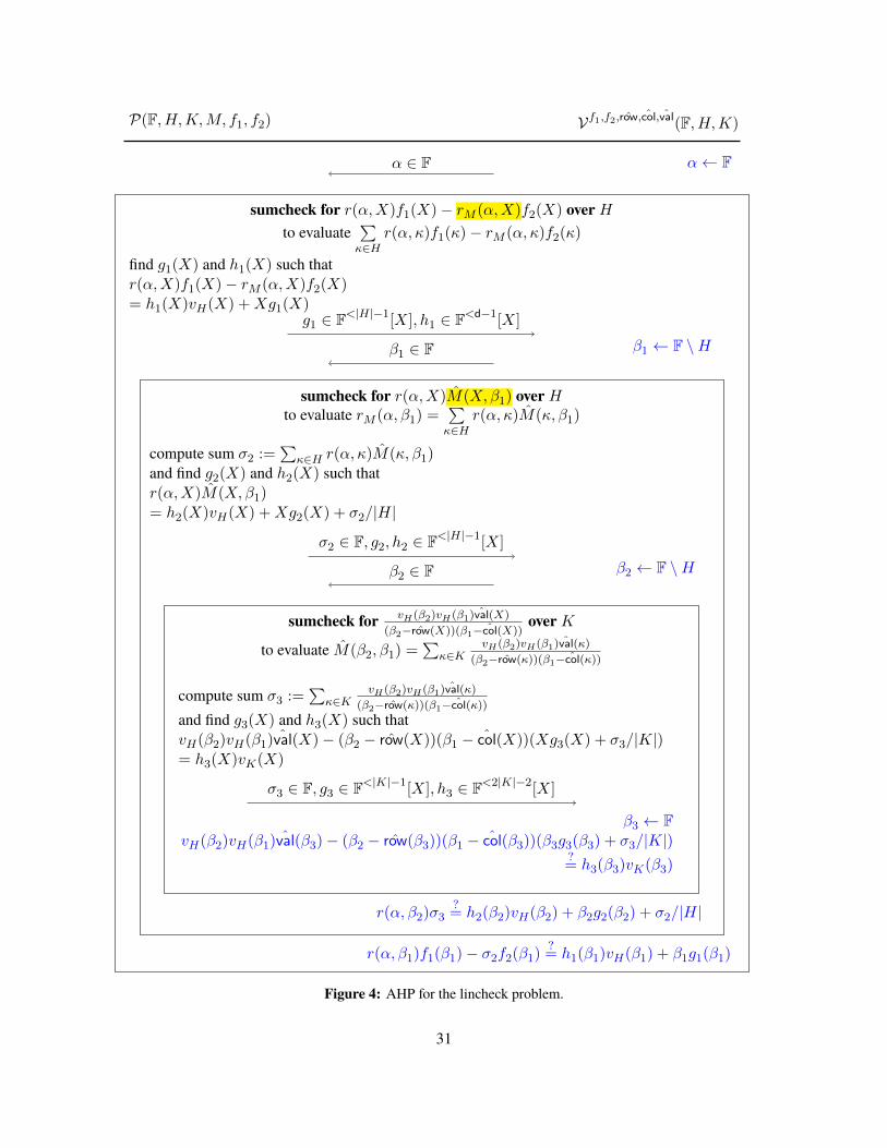
P(F, H,K,M, f1, f2) Vf1,f2, ˆrow,col,val(F, H,K)
α← Fα ∈ F
sumcheck for r(α,X)f1(X)− rM (α,X)f2(X) over Hto evaluate
∑κ∈H
r(α, κ)f1(κ)− rM (α, κ)f2(κ)
find g1(X) and h1(X) such thatr(α,X)f1(X)− rM (α,X)f2(X)= h1(X)vH(X) +Xg1(X)
g1 ∈ F<|H|−1[X], h1 ∈ F<d−1[X]
β1 ← F \Hβ1 ∈ F
sumcheck for r(α,X)M(X,β1) over Hto evaluate rM (α, β1) =
∑κ∈H
r(α, κ)M(κ, β1)
compute sum σ2 :=∑
κ∈H r(α, κ)M(κ, β1)and find g2(X) and h2(X) such thatr(α,X)M(X,β1)= h2(X)vH(X) +Xg2(X) + σ2/|H|
σ2 ∈ F, g2, h2 ∈ F<|H|−1[X]
β2 ← F \Hβ2 ∈ F
sumcheck for vH(β2)vH(β1)val(X)
(β2− ˆrow(X))(β1−col(X))overK
to evaluate M(β2, β1) =∑
κ∈KvH(β2)vH(β1)val(κ)
(β2− ˆrow(κ))(β1−col(κ))
compute sum σ3 :=∑
κ∈KvH(β2)vH(β1)val(κ)
(β2− ˆrow(κ))(β1−col(κ))
and find g3(X) and h3(X) such thatvH(β2)vH(β1)val(X)− (β2 − ˆrow(X))(β1 − col(X))(Xg3(X) + σ3/|K|)= h3(X)vK(X)
σ3 ∈ F, g3 ∈ F<|K|−1[X], h3 ∈ F<2|K|−2[X]
β3 ← FvH(β2)vH(β1)val(β3)− (β2 − ˆrow(β3))(β1 − col(β3))(β3g3(β3) + σ3/|K|)
?= h3(β3)vK(β3)
r(α, β2)σ3?= h2(β2)vH(β2) + β2g2(β2) + σ2/|H|
r(α, β1)f1(β1)− σ2f2(β1)?= h1(β1)vH(β1) + β1g1(β1)
Figure 4: AHP for the lincheck problem.
31
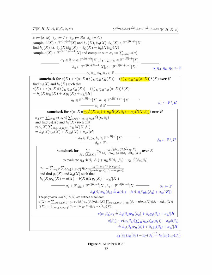
P(F, H,K,A,B,C, x, w) V ˆrowA,B,C,colA,B,C,valA,B,C(F, H,K, x)
z := (x,w) zA := Az zB := Bz zC := Cz
sample w(X) ∈ F<|w|+b[X] and zA(X), zB(X), zC(X) ∈ F<|H|+b[X]find h0(X) s.t. zA(X)zB(X)− zC(X) = h0(X)vH(X)
sample s(X) ∈ F<2|H|+b−1[X] and compute sum σ1 :=∑
κ∈H s(κ)
σ1 ∈ F,w ∈ F<|w|+b[X], zA, zB, zC ∈ F<|H|+b[X],
h0 ∈ F<|H|+2b−1[X], s ∈ F<2|H|+b−1[X] α, ηA, ηB, ηC ← Fα, ηA, ηB, ηC ∈ F
sumcheck for s(X) + r(α,X)(∑
M ηM ˆzM (X))− (∑
M ηMrM (α,X))z(X) over Hfind g1(X) and h1(X) such thats(X) + r(α,X)(
∑M ηM ˆzM (X))− (
∑M ηMrM (α,X))z(X)
= h1(X)vH(X) +Xg1(X) + σ1/|H|
g1 ∈ F<|H|−1[X], h1 ∈ F<|H|+b−1[X]β1 ← F \H
β1 ∈ Fsumcheck for r(α,X)(ηAA(X,β1) + ηBB(X,β1) + ηCC(X,β1)) over H
σ2 :=∑
κ∈H r(α, κ)∑
M∈A,B,C ηMM(κ, β1)and find g2(X) and h2(X) such thatr(α,X)
∑M∈A,B,C ηMM(X,β1)
= h2(X)vH(X) +Xg2(X) + σ2/|H|σ2 ∈ F, g2, h2 ∈ F<|H|−1[X]
β2 ← F \Hβ2 ∈ F
sumcheck for∑
M∈A,B,CηM
vH(β2)vH(β1)valM (X)
(β2− ˆrowM (X))(β1−colM (X))overK
to evaluate ηAA(β2, β1) + ηBB(β2, β1) + ηCC(β2, β1)
σ3 :=∑
κ∈K∑
M∈A,B,C ηMvH(β2)vH(β1)valM (κ)
(β2− ˆrowM (κ))(β1−colM (κ))
and find g3(X) and h3(X) such thath3(X)vK(X) = a(X)− b(X)(Xg3(X) + σ3/|K|)
σ3 ∈ F, g3 ∈ F<|K|−1[X], h3 ∈ F<6|K|−6[X] β3 ← Fh3(β3)vK(β3)
?= a(β3)− b(β3)(β3g3(β3) + σ3/|K|)
The polynomials a(X), b(X) are defined as follows:a(X) :=
∑M∈A,B,C ηMvH(β2)vH(β1)valM (X)
∏N∈A,B,C\M(β2 − ˆrowN (X))(β1 − colN (X))
b(X) :=∏
M∈A,B,C(β2 − ˆrowM (X))(β1 − colM (X))
r(α, β2)σ3?= h2(β2)vH(β2) + β2g2(β2) + σ2/|H|
s(β1) + r(α, β1)(∑
M ηM ˆzM (β1))− σ2z(β1)?= h1(β1)vH(β1) + β1g1(β1) + σ1/|H|
zA(β1)zB(β1)− zC(β1)?= h0(β1)vH(β1)
Figure 5: AHP for R1CS.32

6 Polynomial commitment schemes with extractability
We use polynomial commitment schemes, a class of commitment schemes specialized to work with univariatepolynomials. This notion was introduced by Kate, Zaverucha, and Goldberg [KZG10], who gave an elegantconstruction using bilinear groups. The security properties in [KZG10], however, do not appear sufficient forstandalone use (nor for use in this paper). This limitation was recently noted in [Mal+19], which relies on adifferent construction for which certain properties are proved in the algebraic group model [FKL18]. However,[Mal+19] stops short of formulating a cryptographic primitive that captures the features of the construction.
In this sectionwe propose definitions for polynomial commitment schemes that incorporate the functionalityand security that we believe to be a bare minimum for standalone use. (In particular, in Section 8 we genericallyrely on these definitions to build preprocessing arguments with universal SRS.) We also describe a “knowledge”variant of the construction in [KZG10], which we prove secure under knowledge of exponent assumptions. Tolearn more about the insights motivating our definitions, we refer the reader back to Section 2.2.
The rest of this section is organized as follows. In Section 6.1 we present the definitions that we propose.In Section 6.2 we provide a theorem statement for constructions that realize the definitions, and then sketchthese constructions. We formal descriptions of the constructions are in Appendices B to C.
6.1 Definition
A polynomial commitment scheme over a field familyF is a tuple of algorithms PC = (Setup,Trim,Commit,Open,Check) with the following syntax.
• PC.Setup(1λ, D)→ pp. On input a security parameter λ (in unary), and a maximum degree boundD ∈ N,PC.Setup samples public parameters pp. The parameters contain the description of a finite field F ∈ F .
• PC.Trimpp(1λ,d) → (ck, rk). Given oracle access to public parameters pp, and on input a securityparameter λ (in unary), and degree bounds d, PC.Trim deterministically computes a key pair (ck, rk) thatis specialized to d.
• PC.Commit(ck,p,d;ω) → c. On input ck, univariate polynomials p = [pi]ni=1 over the field F, and
degree bounds d = [di]ni=1 with deg(pi) ≤ di ≤ D, PC.Commit outputs commitments c = [ci]
ni=1 to the
polynomials p = [pi]ni=1. The randomness ω = [ωi]
ni=1 is used if the commitments c = [ci]
ni=1 are hiding.
• PC.Open(ck,p,d, Q, ξ;ω) → π. On input ck, univariate polynomials p = [pi]ni=1, degree bounds
d = [di]ni=1, a query setQ consisting of tuples (i, z) ∈ [n]× F, and opening challenge ξ, PC.Open outputs
an evaluation proof π. The randomness ω must equal the one previously used in PC.Commit.
• PC.Check(rk, c,d, Q,v, π, ξ) ∈ 0, 1. On input rk, commitments c = [ci]ni=1, degree bounds d = [di]
ni=1,
query set Q consisting of tuples (i, z) ∈ [n]× F, alleged evaluations v = (v(i,z))(i,z)∈Q, evaluation proofπ, and opening challenge ξ, PC.Check outputs 1 if π attests that, for every (i, z) ∈ Q, the polynomial picommitted in ci has degree at most di and evaluates to v(i,z) at z.
A polynomial commitment scheme PC must satisfy the completeness and extractability properties definedbelow. We also consider two additional properties, succinctness and hiding, also defined below. To simplifynotation, we denote by deg(p) the degrees [deg(pi)]
ni=1 of polynomials p = [pi]
ni=1, and denote by p(Q) the
evaluations (pi(z))(i,z)∈Q of the polynomials p = [pi]ni=1 at a query set Q ⊆ [n]× F.
33

Definition 6.1 (Completeness). For every maximum degree bound D ∈ N and efficient adversary A,
Pr
deg(p) ≤ d ≤ D
⇓PC.Check(rk, c,d, Q,v, π, ξ) = 1
∣∣∣∣∣∣∣∣∣∣∣∣∣
pp← PC.Setup(1λ, D)(p,d, Q, ξ,ω)← A(pp)
(ck, rk)← PC.Trimpp(1λ,d)c← PC.Commit(ck,p,d;ω)
v ← p(Q)π ← PC.Open(ck,p,d, Q, ξ;ω)
= 1 .
Definition 6.2 (Extractability). For every maximum degree bound D ∈ N and efficient adversary A thereexists an efficient extractor E such that for every round bound r ∈ N, efficient public-coin challenger C (eachof its messages is a uniformly random string of prescribed length, or an empty string), efficient query samplerQ, and efficient adversary B = (B1,B2) the probability below is negligibly close to 1 (as a function of λ):
Pr
PC.Check(rk, c,d, Q,v, π, ξ) = 1
⇓
deg(p) ≤ d ≤ D and v = p(Q)
∣∣∣∣∣∣∣∣∣∣∣∣∣∣∣∣∣∣∣∣∣∣∣∣∣∣
pp← PC.Setup(1λ, D)
For i = 1, . . . , r:ρi ← C(pp, i)
(ci,di)← A(pp, [ρj ]ij=1)
pi ← E(pp, [ρj ]ij=1)
Q← Q(pp, [ρj ]rj=1)
(v, st)← B1(pp, [ρj ]rj=1, Q)
Sample opening challenge ξπ ← B2(st, ξ)
Set [ci]ni=1 := [ci]
ri=1, [pi]
ni=1 := [pi]
ri=1, [di]
ni=1 := [di]
ri=1
(ck, rk)← PC.Trimpp(1λ, [di]ni=1)
Define the set of queried polynomials T := i ∈ [n] | (i, z) ∈ QSet c := [ci]i∈T ,p := [pi]i∈T ,d := [di]i∈T
.
(The above definition captures the case where A,Q,B share the same random string to win the game.)
Definition 6.3 (Efficiency). We say that a polynomial commitment scheme PC is:• degree-efficient if the time to run PC.Commit and PC.Open is proportional to the maximum degree max(d)(as opposed to the maximum supported degree D). In particular this implies that |ck| = Oλ(max(d)).
• succinct if the size of commitments, the size of evaluation proofs, and the time to check an opening are allindependent of the degree of the committed polynomials. That is, |c| = n · poly(λ), |π| = |Q| · poly(λ),|rk| = Oλ(n), and time(Check) = (n+ |Q|) · poly(λ).
Definition 6.4 (Hiding). There exists a polynomial-time simulator S = (Setup,Commit,Open) such that,for every maximum degree bound D ∈ N, and efficient adversary A = (A1,A2,A3), the probability thatb = 1 in the following two experiments is identical:
34

Real(1λ, D,A):1. pp← PC.Setup(1λ, D).2. Letting c0 := ⊥, for i = 1, . . . , r:
(a) (pi,di, hi)← A1(pp, c0, c1, . . . , ci−1).(b) (cki, rki)← PC.Trimpp(1λ,di).(c) If hi = 0: sample commitment randomness ωi.(d) If hi = 1: set randomness ωi to ⊥.(e) ci ← PC.Commit(cki,pi,di;ωi).
3. c := [ci]ri=1,p := [pi]
ri=1,d := [di]
ri=1,ω := [ωi]
ri=1.
4. (ck, rk)← PC.Trimpp(1λ,d).5. ([Qj ]
τj=1, [ξj ]
τj=1, st)← A2(pp, c).
6. For j ∈ [τ ]:πj ← PC.Open(ck,p,d, Qj , ξj ;ω).
7. b← A3(st, [π]τj=1).
Ideal(1λ, D,A):1. (pp, trap)← S.Setup(1λ, D).2. Letting c0 := ⊥, for i = 1, . . . , r:
(a) (pi,di, hi)← A1(pp, c0, c1, . . . , ci−1).(b) (cki, rki)← PC.Trimpp(1λ,di).(c) If hi = 0: sample randomnessωi and compute simu-
lated commitments ci ← S.Commit(trap,di;ωi).(d) If hi = 1: set ωi := ⊥ and compute (real) commit-
ments ci ← PC.Commit(cki,pi,di;ωi).3. c := [ci]
ri=1,p := [pi]
ri=1,d := [di]
ri=1,ω := [ωi]
ri=1.
4. (ck, rk)← PC.Trimpp(1λ,d).5. ([Qj ]
τj=1, [ξj ]
τj=1, st)← A2(pp, c).
6. Zero out hidden polynomials: p′ := [hipi]ri=1.
7. For j ∈ [τ ]:πj ← S.Open(trap,p′,p(Qj),d, Qj , ξj ;ω).
8. b← A3(st, [π]τj=1).
(We implicitly assume that A1 outputs poly(λ) polynomials overall and that A2 outputs poly(λ) query setseach consisting of poly(λ) points, ensuring that PCs.Commit,PCs.Open,S.Commit,S.Open are efficient.)
6.2 Construction
The theorem below states the properties of our constructions. For simplicity, our construction are restricted towork with respect to “admissible” query samplers.
Definition 6.5. A query sampler Q is admissible if it outputs query sets such that each polynomial to beevaluated is evaluated at a point sampled uniformly at random from a super-polynomially large subset of thefield, and possibly also at other points that can be arbitrarily chosen.
Theorem 6.6. There exist succinct polynomial commitment schemes that: (a) achieve extractability againstadmissible query samplers under knowledge assumptions, or in the algebraic group model; (b) achieve hiding;and (c) have an updatable SRS. See Table 2 for the efficiency of these schemes under these assumptions.
We note that the restriction to admissible query samplers is minor because one can transform an arbitraryquery sampler Q into an admissible query sampler Q′ as follows: Q′ invokes Q to obtain a query set Q,and then outputs Q′ := Q ∪ (i, t)i∈[n], where t ∈ F is a random field element and n is the number ofpolynomials. This transformation yields evaluation proofs that are twice as a large, a minor cost. That said,this transformation is often not even needed because “natural” query samplers are often already admissible,as is the case for those that we consider in this paper.
single-bound single-querypolynomial commitment
(Appendix B)
multiple-bound single-querypolynomial commitment
(Appendix C)
multiple-bound multiple-querypolynomial commitment
(Appendix D)
Figure 6: Our approach to construct polynomial commitment schemes.
The constructions behind Theorem 6.6 are achieved in three steps, as summarized in Fig. 6. The restof this section is organized in three parts sketching these three steps respectively: (1) opening multiplepolynomials with the same degree bound at a single point; (2) opening multiple polynomials with multipledegree bounds at a single point; (3) opening multiple polynomials with multiple degree bounds at multiplepoints. Detailed descriptions, along with security proofs, are provided in the corresponding appendices.
35
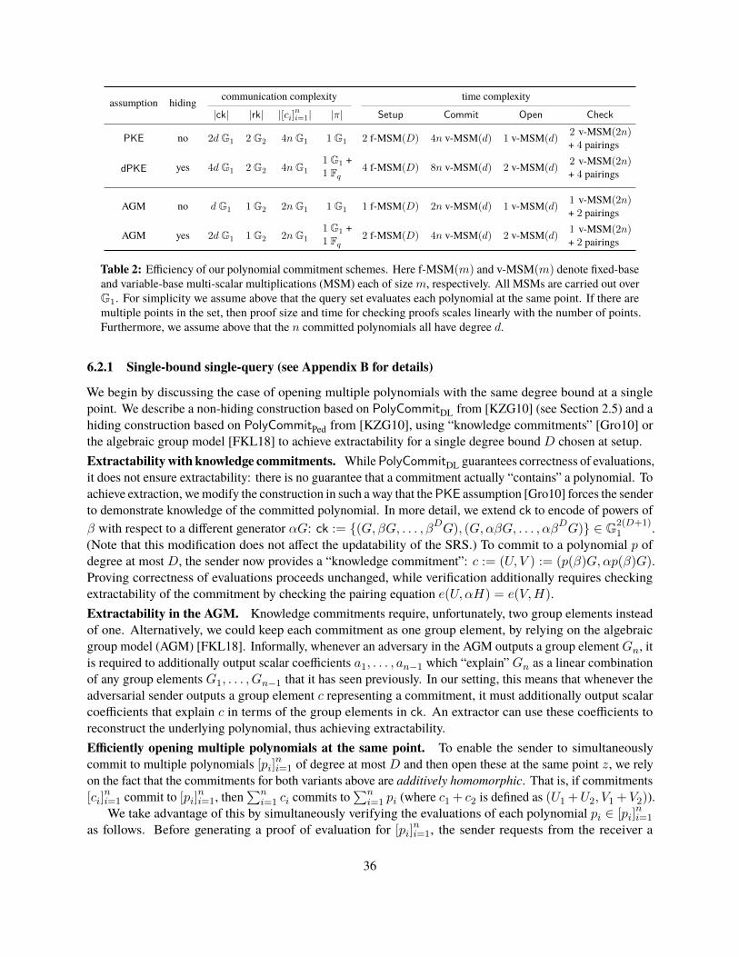
assumption hiding communication complexity time complexity
|ck| |rk| |[ci]ni=1| |π| Setup Commit Open Check
PKE no 2d G1 2 G2 4n G1 1 G1 2 f-MSM(D) 4n v-MSM(d) 1 v-MSM(d)2 v-MSM(2n)+ 4 pairings
dPKE yes 4d G1 2 G2 4n G1
1 G1 +1 Fq
4 f-MSM(D) 8n v-MSM(d) 2 v-MSM(d)2 v-MSM(2n)+ 4 pairings
AGM no d G1 1 G2 2n G1 1 G1 1 f-MSM(D) 2n v-MSM(d) 1 v-MSM(d)1 v-MSM(2n)+ 2 pairings
AGM yes 2d G1 1 G2 2n G1
1 G1 +1 Fq
2 f-MSM(D) 4n v-MSM(d) 2 v-MSM(d)1 v-MSM(2n)+ 2 pairings
Table 2: Efficiency of our polynomial commitment schemes. Here f-MSM(m) and v-MSM(m) denote fixed-baseand variable-base multi-scalar multiplications (MSM) each of sizem, respectively. All MSMs are carried out overG1. For simplicity we assume above that the query set evaluates each polynomial at the same point. If there aremultiple points in the set, then proof size and time for checking proofs scales linearly with the number of points.Furthermore, we assume above that the n committed polynomials all have degree d.
6.2.1 Single-bound single-query (see Appendix B for details)
We begin by discussing the case of opening multiple polynomials with the same degree bound at a singlepoint. We describe a non-hiding construction based on PolyCommitDL from [KZG10] (see Section 2.5) and ahiding construction based on PolyCommitPed from [KZG10], using “knowledge commitments” [Gro10] orthe algebraic group model [FKL18] to achieve extractability for a single degree bound D chosen at setup.Extractability with knowledge commitments. WhilePolyCommitDL guarantees correctness of evaluations,it does not ensure extractability: there is no guarantee that a commitment actually “contains” a polynomial. Toachieve extraction, wemodify the construction in such a way that thePKE assumption [Gro10] forces the senderto demonstrate knowledge of the committed polynomial. In more detail, we extend ck to encode of powers ofβ with respect to a different generator αG: ck := (G, βG, . . . , βDG), (G,αβG, . . . , αβDG) ∈ G2(D+1)
1 .(Note that this modification does not affect the updatability of the SRS.) To commit to a polynomial p ofdegree at most D, the sender now provides a “knowledge commitment”: c := (U, V ) := (p(β)G,αp(β)G).Proving correctness of evaluations proceeds unchanged, while verification additionally requires checkingextractability of the commitment by checking the pairing equation e(U,αH) = e(V,H).Extractability in the AGM. Knowledge commitments require, unfortunately, two group elements insteadof one. Alternatively, we could keep each commitment as one group element, by relying on the algebraicgroup model (AGM) [FKL18]. Informally, whenever an adversary in the AGM outputs a group elementGn, itis required to additionally output scalar coefficients a1, . . . , an−1 which “explain” Gn as a linear combinationof any group elements G1, . . . , Gn−1 that it has seen previously. In our setting, this means that whenever theadversarial sender outputs a group element c representing a commitment, it must additionally output scalarcoefficients that explain c in terms of the group elements in ck. An extractor can use these coefficients toreconstruct the underlying polynomial, thus achieving extractability.Efficiently opening multiple polynomials at the same point. To enable the sender to simultaneouslycommit to multiple polynomials [pi]
ni=1 of degree at most D and then open these at the same point z, we rely
on the fact that the commitments for both variants above are additively homomorphic. That is, if commitments[ci]
ni=1 commit to [pi]
ni=1, then
∑ni=1 ci commits to
∑ni=1 pi (where c1 + c2 is defined as (U1 +U2, V1 +V2)).
We take advantage of this by simultaneously verifying the evaluations of each polynomial pi ∈ [pi]ni=1
as follows. Before generating a proof of evaluation for [pi]ni=1, the sender requests from the receiver a
36

random field element ξ. The sender then uses this to take a random linear combination of the polynomials:p :=
∑ni=1 ξ
ipi, and generates a single evaluation proof π for this derived polynomial p.To verify π, the receiver uses the additive homomorphism of the input commitments to derive the linear
combination c =∑n
i=1 ξici induced by ξ. It does the same with the claimed evaluations, thus deriving the
evaluation v =∑n
i=1 ξivi. Finally, it checks that the pairing equations are satisfied for c, π, and v.
This works because if the sender is honest, then c is a commitment to p :=∑n
i=1 ξipi, and π is a proof of
evaluation of p at z. On the other hand, if the sender is dishonest, then with high probability over the choiceof ξ, c is not a commitment to p, and the pairing equations would fail.Hiding. To additionally achieve hiding, we follow the above blueprint, replacing PolyCommitDL with thehiding scheme PolyCommitPed. Extraction now follows from an assumption related to PKE called dPKE (seeAppendix B.2.3 for details). Our constructions in Appendix B in fact use both variants to provide optionalhiding on a per-polynomial basis. Further, the near-identical form of the commitment variants makes itpossible to open a combination of hiding and non-hiding polynomials at the same point.
6.2.2 Multiple-bound single-query (see Appendix C for details)
Thus far, we have focused on commitment schemes for polynomials of degreeD where the cost of committingand providing evaluation proofs grows as Ω(D). However, when working with polynomials of degree d < D,we would like to pay a cost that instead grows as O(d). Furthermore, the foregoing schemes only guaranteethat committed polynomials have degree at most D, whereas in many cases it is desirable to enforce morespecific degree bounds. Below we show how to adapt the foregoing construction to achieve these desirableproperties.
To achieve extractability with respect to a different degree bound di for each polynomial pi, we requirethe sender to commit not only to each pi, but also to “shifted polynomials” p′i(X) := XD−dipi(X). DuringPC.Open, one could then produce an evaluation proofs that attests that if pi evaluates to vi at z then p′ievaluates to zD−divi at z.
The receiver checks that the commitment for each p′i corresponds to an evaluation zD−divi so that, if z issampled from a super-polynomial subset of Fq, the probability that deg(pi) 6= di is negligible. This trick issimilar to the one used in [BS08; Ben+19c] to enforce derive low-degree tests for specific degree bounds.
However, while sound, this approach is inefficient in our setting: the witness polynomial for p′i hasΩ(D) non-zero coefficients (instead of O(di)), and so constructing an evaluation proof for it requires Ω(D)scalar multiplications (instead of O(di)). To work around this, we instead produce a proof that the relatedpolynomial p?i (X) := p′i(X) − pi(z)X
D−di evaluates to 0 at z. As we show in Lemma C.2, the witnesspolynomial for this claim has O(di) non-zero coefficients, and so constructing the evaluation proof can bedone in O(di) scalar multiplications. Completeness is preserved because the receiver can check the correctevaluation of p?i by subtracting pi(z)(β
D−diG) from the commitment to the shifted polynomial p′i, therebyobtaining a commitment to p?i , while security is preserved because p
′i(z) = zD−divi ⇐⇒ p?i (z) = 0.
Note that to commit to the shifted polynomial p′i, the committer must obtain βD−diG, . . . , βDG fromck, while to adjust the shifted commitment, the receiver must obtain βD−diG from rk. Thus PC.Trim mustproduce (ck, rk) containing these group elements.
6.2.3 Multiple-bound multiple-query (see Appendix D for details)
Assume that we have any construction that achieves extractability with respect to individual degree bounds,and evaluation of multiple polynomials p = [pi]
ni=1 at the same point z.
37

We extend this construction to support query sets Q consisting of multiple evaluation points (as requiredin Section 6.1). If there are k distinct points [zi]
ki=1 in the query set Q, the sender partitions the polynomials
p into different (possibly overlapping) groups [pi]ki=1 such that every polynomial in pi is to be evaluated at
the same point zi. It then runs PC.Open on each pi, and outputs the resulting list of k evaluation proofs.We note that [KZG10] describe how one can enable the sender to produce a single evaluation proof
attesting to the correct evaluation of the same polynomial at multiple points. While we could use this toenable batch evaluation of p at multiple points, we avoid doing so for efficiency reasons in our setting.
38
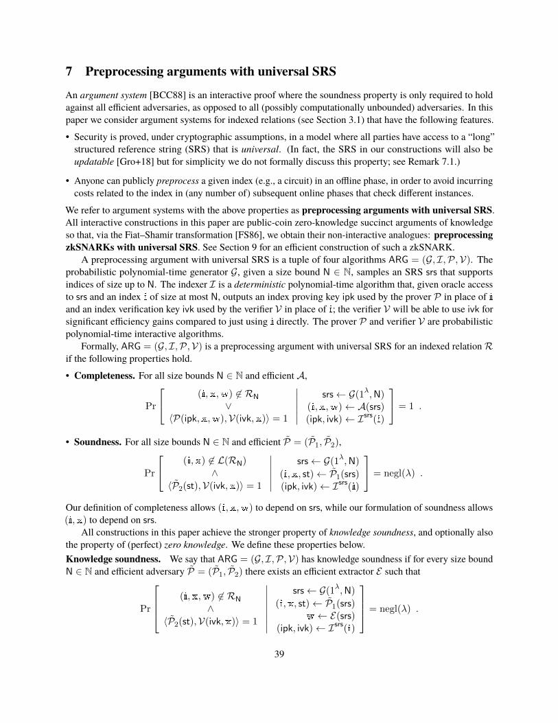
7 Preprocessing arguments with universal SRS
An argument system [BCC88] is an interactive proof where the soundness property is only required to holdagainst all efficient adversaries, as opposed to all (possibly computationally unbounded) adversaries. In thispaper we consider argument systems for indexed relations (see Section 3.1) that have the following features.
• Security is proved, under cryptographic assumptions, in a model where all parties have access to a “long”structured reference string (SRS) that is universal. (In fact, the SRS in our constructions will also beupdatable [Gro+18] but for simplicity we do not formally discuss this property; see Remark 7.1.)
• Anyone can publicly preprocess a given index (e.g., a circuit) in an offline phase, in order to avoid incurringcosts related to the index in (any number of) subsequent online phases that check different instances.
We refer to argument systems with the above properties as preprocessing arguments with universal SRS.All interactive constructions in this paper are public-coin zero-knowledge succinct arguments of knowledgeso that, via the Fiat–Shamir transformation [FS86], we obtain their non-interactive analogues: preprocessingzkSNARKs with universal SRS. See Section 9 for an efficient construction of such a zkSNARK.
A preprocessing argument with universal SRS is a tuple of four algorithms ARG = (G, I,P,V). Theprobabilistic polynomial-time generator G, given a size bound N ∈ N, samples an SRS srs that supportsindices of size up to N. The indexer I is a deterministic polynomial-time algorithm that, given oracle accessto srs and an index i of size at most N, outputs an index proving key ipk used by the prover P in place of iand an index verification key ivk used by the verifier V in place of i; the verifier V will be able to use ivk forsignificant efficiency gains compared to just using i directly. The prover P and verifier V are probabilisticpolynomial-time interactive algorithms.
Formally, ARG = (G, I,P,V) is a preprocessing argument with universal SRS for an indexed relationRif the following properties hold.
• Completeness. For all size bounds N ∈ N and efficient A,
Pr
(i,x,w) 6∈ RN
∨〈P(ipk,x,w),V(ivk,x)〉 = 1
∣∣∣∣∣∣srs← G(1λ,N)
(i,x,w)← A(srs)(ipk, ivk)← Isrs(i)
= 1 .
• Soundness. For all size bounds N ∈ N and efficient P = (P1, P2),
Pr
(i,x) 6∈ L(RN)∧
〈P2(st),V(ivk,x)〉 = 1
∣∣∣∣∣∣srs← G(1λ,N)
(i,x, st)← P1(srs)(ipk, ivk)← Isrs(i)
= negl(λ) .
Our definition of completeness allows (i,x,w) to depend on srs, while our formulation of soundness allows(i,x) to depend on srs.
All constructions in this paper achieve the stronger property of knowledge soundness, and optionally alsothe property of (perfect) zero knowledge. We define these properties below.Knowledge soundness. We say that ARG = (G, I,P,V) has knowledge soundness if for every size boundN ∈ N and efficient adversary P = (P1, P2) there exists an efficient extractor E such that
Pr
(i,x,w) 6∈ RN
∧〈P2(st),V(ivk,x)〉 = 1
∣∣∣∣∣∣∣∣srs← G(1λ,N)
(i,x, st)← P1(srs)w← E(srs)
(ipk, ivk)← Isrs(i)
= negl(λ) .
39

Zero knowledge. We say that ARG = (G, I,P,V) has (perfect) zero knowledge if there exists an efficientsimulator S = (Setup,Prove) such that for every efficient adversary V = (V1, V2) it holds that
Pr
(i,x,w) ∈ RN
∧〈P(ipk,x,w), V2(st)〉 = 1
∣∣∣∣∣∣srs← G(1λ,N)
(i,x,w, st)← V1(srs)(ipk, ivk)← Isrs(i)
= Pr
(i,x,w) ∈ RN
∧〈S.Prove(trap, i,x), V2(st)〉 = 1
∣∣∣∣∣∣ (srs, trap)← S.Setup(1λ,N)
(i,x,w, st)← V1(srs)
.
Efficiency. We say that ARG = (G, I,P,V) is:• index efficient if the running time of the prover P(ipk,x,w) is polyλ(|i|), i.e., it does not depend on thesize of the universal structured reference string srs;
• proof succinct if the size of the communication transcript between the prover P(ipk,x,w) and verifierV(ivk,x) is poly(λ), i.e., the size is bounded by a universal polynomial in the security parameter λ;
• verifier succinct if the running time of V(ivk,x) is poly(λ+ |x|), i.e., the time is bounded by a universalpolynomial in the security parameter λ and the size of the instance x and does not depend on the size of theindex i that led to ivk.
Index efficiency implies that ipk output by I is of size polyλ(|i|), while verifier succinctness implies that ivkoutput by I is of size poly(λ). All constructions in this paper are index efficient, proof succinct, and verifiersuccinct.Public coins. We say that ARG = (G, I,P,V) is public-coin if every message output by the verifier V is auniform random string of some prescribed length. All constructions in this paper are public-coin, and have a(small) constant number of rounds; in particular, they can be “squashed” to non-interactive arguments that arepublicly verifiable by additionally using random oracles via the Fiat–Shamir transformation [FS86]. Hence,due to their succinctness, our constructions directly lead to preprocessing zkSNARKs with universal SRS.
Remark 7.1 (updatable SRS). An SRS is updatable [Gro+18] if there exists an update algorithm that can berun at any time by anyone to update the SRS, with the guarantee that security holds as long as there is atleast one honest updater since the beginning of time. This property significantly simplifies cryptographicceremonies to sample the SRS. All preprocessing arguments that we construct in this paper have updatableSRS because they only contain “monomial terms”, and thus fall within the framework of [Gro+18].
Remark 7.2 (auxiliary inputs). The definition of knowledge soundness above does not consider auxiliaryinputs, for simplicity. One could consider a stronger definition, where the adversary and extractor additionallyreceive an auxiliary input z sampled from a fixed distribution Z(1λ), or even sampled from any distributionZ(1λ) that belongs to a given class. Such stronger definitions are useful when using argument systemsas subroutines within other protocols. When relying on auxiliary inputs, however, one must be carefulto ensure that they come from “benign” distributions, or else extraction is impossible, as discussed in[BP15; Bit+16]. We stress that all of our constructions of argument systems directly extend to hold withrespect to an auxiliary-input distribution Z(1λ) under the assumption that the relevant underlying knowledgeassumptions are extended to hold with respect to the auxiliary-input distribution Z(1λ) concatenated withsome randomness. (In other words, our security reduction adds to the auxiliary input some random strings.)
40

8 From AHPs to preprocessing arguments with universal SRS
The following theorems capture key properties of our compiler.
Theorem 8.1. Let F be a field family and letR be an indexed relation. Consider the following components:– AHP = (k, s, d, I,P,V) is an AHP over F forR with negligible soundness error (see Section 4);– PC = (Setup,Trim,Commit,Open,Check) is a polynomial commitment scheme over F (see Section 6).Then ARG = (G, I,P,V) described in Section 8.1 is a preprocessing argument with universal SRS for R(see Section 7). Moreover, if q is the query complexity of AHP, ARG has the following efficiency:• round complexity is k + 2;• communication complexity is Oλ(q) bits if PC is additionally succinct (see Definition 6.3);• indexer time is the sum of the indexer time in AHP and the time to commit to s(0) polynomials in PC;• prover time is the sum of the prover time in AHP, the time to commit to
∑ki=1 s(i) polynomials in PC, the
time to produce evaluations that answer the q queries along with a batch evaluation proof for them in PC;• verifier time is the sum of the verifier time in AHP and the time to batch verify q evaluations in PC.
Remark 8.2 (updatable SRS). If the SRS for PC is updatable then so is the SRS for ARG. All constructionsof polynomial commitments in this paper satisfy this property, including the one used in Section 9.
The construction underlying the above theorem preserves knowledge soundness and, if the polynomialcommitment scheme is also hiding, preserves zero knowledge.
Theorem 8.3. In Theorem 8.1, if AHP has a negligible knowledge soundness error, then ARG has knowledgesoundness.
Theorem 8.4. In Theorem 8.1, if PC is hiding and if AHP is zero knowledge with query bound q (the querycomplexity of AHP) and some polynomial-time query checker C, then ARG is (perfect) zero knowledge.
Remark 8.5 (the multivariate case). In this paper we give definitions for algebraic holographic proofs andpolynomial commitment schemes that are restricted to the case of univariate polynomials, because theconstructions that we consider are univariate. Theorems 8.1, 8.3 and 8.4, however, directly extend to themultivariate case when considering an AHP in the general case of multivariate polynomials and a polynomialcommitment scheme for multivariate polynomials. This provides a proof of security for several prior worksthat considered constructions that are special cases of this paradigm but did not prove security (because thepolynomial commitment schemes were only assumed to satisfy evaluation binding as discussed in Section 1.2).
8.1 Construction
We describe the construction behind Theorem 8.1, and then discuss its efficiency features.Generator G. The generator G, on input a security parameter λ ∈ N and size bound N ∈ N, uses N tocompute a maximum degree bound D ∈ N, samples public parameters pp ← PC.Setup(1λ, D) for thepolynomial commitment scheme PC, and then outputs srs := pp. The integer D is computed to be themaximum degree bound in AHP for indices of size N. In other words,
D := maxd(N, i, j)
∣∣∣ i ∈ 0, 1, . . . , k(N) , j ∈ 1, . . . , s(i). (9)
Indexer I . The indexer I upon input i and given oracle access to srs, deduces the field F ∈ F contained insrs = pp, runs the AHP indexer I on (F, i) to obtain s(0) polynomials p0,1, . . . , p0,s(0) ∈ F[X] of degrees
41

at most d(|i|, 0, 1), . . . , d(|i|, 0, s(0)), computes the degree bounds for the index and prover polynomials,invokes PC.Trim on these bounds to compute (ck, rk) that are specialized for these degree bounds, andcomputes commitments to all of the index polynomials.
Namely, I calculates the bounds d := d(|i|, i, s(i))k(|i|)i=0 , invokes (ck, rk) := PC.Trimsrs(d), and
then computes [c0,j ]s(0)j=1 := PC.Commit(ck, [p0,j ]
s(0)j=1, [d(|i|, 0, j)]s(0)
j=1; [ω0,j ]s(0)j=1) for “empty randomness”
[ω0,j ]s(0)j=1 := ⊥. The indexer I outputs ipk := (ck, i, [p0,j ]
s(0)j=1, [c0,j ]
s(0)j=1) and ivk := (rk, [c0,j ]
s(0)j=1). (Note
that [c0,j ]s(0)j=1 are commitments to non-secret information so no randomness is used in producing them. In
particular, I is a deterministic polynomial-time algorithm, as required. Also see Remark 8.6 below foradditional considerations.)Prover P and verifier V . The prover P receives (ipk,x,w) and the verifier V receives (ivk,x), where(ipk, ivk) is the index key pair output by Isrs(i), and (i,x,w) is in the indexed relationR. By construction ofI, ipk contains a trimmed committer key ck and ivk contains a trimmed receiver key rk for the polynomialcommitment scheme PC. Let F ∈ F be the field described by (ck, rk) (each of ck and rk individually containa description of F), and let k := k(|i|) be the number of rounds in AHP. For i ∈ 1, . . . , k, P and V simulatethe i-th round of the interaction between the AHP prover P(F, i,x,w) and the AHP verifier V(F,x).
1. V receives ρi ∈ F∗ from V, and forwards it to P .2. P forwards ρi to P, which replies with polynomials pi,1, . . . , pi,s(i) ∈ F[X] with deg(pi,j) ≤ d(|i|, i, j).3. P samples commitment randomness [ωi,j ]
s(i)j=1 and sends to V the polynomial commitments below
[ci,j ]s(i)j=1 := PC.Commit(ck, [pi,j ]
s(i)j=1, [d(|i|, i, j)]s(i)j=1; [ωi,j ]
s(i)j=1) .
4. V notifies V that the i-th round has finished.
The proverP and verifier V are done simulating the interactive phase of AHP, and in the remaining two roundssimulate the (non-adaptive) query phase of AHP. Below we use c to denote the commitments [[ci,j ]
s(i)j=1]ki=0, p
to denote the polynomials [[pi,j ]s(i)j=1]ki=0, d to denote the degree bounds [[d(|i|, i, j)]s(i)j=1]ki=0, and ω to denote
the randomness [[ωi,j ]s(i)j=1]ki=0 with [ω0,j ]
s(0)j=1 := ⊥. Note that these three vectors include the commitments,
polynomials, degrees, and randomness of the “0-th round”.
• V sends a message ρk+1 ∈ F∗ that represents randomness for the query phase of V(F,x) to P .• P uses the query algorithm of V to compute the query set Q := QV(F,x; ρ1, . . . , ρk, ρk+1).• P replies with answers v := p(Q).• V samples and sends an opening challenge ξ ∈ F to P .• P replies with an evaluation proof to demonstrate correctness of all claimed evaluations:
π := PC.Open(ck,p,d, Q, ξ;ω) .
• V accepts if and only if the following conditions hold:– the decision algorithm of V accepts the answers, i.e., DV(F,x,v; ρ1, . . . , ρk, ρk+1) = 1;– the alleged answers pass the test, i.e., PC.Check(rk, c,d, Q,v, π, ξ) = 1.
Completeness of the preprocessing argument ARG follows in a straightforward way from completeness ofthe AHP AHP and completeness of the polynomial commitment scheme PC.
We now discuss the efficiency features of the construction above.
42

• Round complexity. The first k rounds simulate the interactive phase of AHP, with polynomials sent ascommitments; one round is to answer the desired queries; and one round is to certify the queries’ answers.
• Communication complexity. The argument prover P sends∑k
i=1 s(i) commitments, q field elementsrepresenting query answers, and an evaluation proof that certifies the q answers. The argument verifierV sends |ρ1|+ · · ·+ |ρk|+ |ρk+1|+ 1 field elements. In Theorem 8.1 we state that the communicationcomplexity is Oλ(q) because typically it holds that
∑ki=0 s(i) ≤ q (each polynomial is queried at least
once) and |ρ1|+ · · ·+ |ρk|+ |ρk+1| is a small constant (each verifier message is a few field elements).• Indexer time. The time complexity of I equals the time complexity of the AHP indexer I plus the time totrim the PC public parameters pp, and then to commit to the s(0) polynomials output by I.
• Prover time. The time complexity of P equals the time complexity of the AHP prover P plus the time tocommit to the
∑ki=1 s(i) polynomials output by P, evaluate
∑ki=0 s(i) polynomials at the query set Q, and
produce an evaluation proof that certifies the correctness of these evaluations.• Verifier time. The time complexity of V equals the time complexity of the AHP verifier V plus the time toverify the batch evaluation proof for the q evaluations that provide answers to the query set Q.
Remark 8.6 (commitments to index polynomials). The construction described above uses the same polynomialcommitment scheme PC for committing to polynomials output by the AHP indexer and to polynomials outputby the AHP prover. This simplifies exposition, and allows for a single evaluation proof to certify all queryanswers. For security, however, it would suffice (even for Theorem 8.4) to commit to index polynomials via acommitment scheme that merely satisfies “evaluation binding” (Definition B.8), which is strictly weaker thanthe notion of extractability that we use for the other commitments. This is because the commitments in theindex verification key are honestly produced in the preprocessing phase. Moreover, for Theorem 8.3 to holdwe do not need the commitments to index polynomials to be hiding.
8.2 Proof of Theorem 8.1
Suppose that P = (P1, P2) is an efficient adversarial prover for ARG that wins with probability at least ε,that is,
Pr
(i,x) 6∈ L(RN)∧
〈P2(st),V(ivk,x)〉 = 1
∣∣∣∣∣∣srs← G(1λ,N)
(i,x, st)← P1(srs)(ipk, ivk)← Isrs(i)
≥ ε(λ) .
We assume without loss of generality that st output by P1 contains the public parameters srs = pp. Also notethat P2 can be represented via its k + 2 next-message functions:
P2(st; ρ1) , P2(st; ρ1, ρ2) , . . . , P2(st; ρ1, . . . , ρk) , P2(st; ρ1, . . . , ρk, Q) , P2(st; ρ1, . . . , ρk, Q, ξ) .
We describe how to construct a prover P, which is admissible for AHP, and an efficient adversaryAPC againstthe extractability of PC such that
Pr
(i,x) 6∈ L(RN)∧
〈P(st),VI(F,i)(F,x)〉 = 1
∣∣∣∣∣∣pp← PC.Setup(1λ, D)
F← field(pp)
(i,x, st)← P1(pp)
+ Pr
[APC wins the
extractability game
]≥ ε(λ) ,
Above, D is computed according to Eq. (9) and F is the field described in pp. This concludes the proofbecause if ε(λ) were to be non-negligible then either: (i) by averaging there would exist a choice of publicparameters pp that yields a state st, field F ∈ F , and (i,x) 6∈ L(R) for which Pr[〈P(st),VI(F,i)(F,x)〉 = 1]
43

is non-negligible, contradicting our hypothesis AHP has negligible soundness error; or (ii) there would existan efficient adversary APC that, for any given efficient extractor, succeeds in the extractability game for PC(Definition 6.2) with non-negligible probability, contradicting our hypothesis PC is extractable.ConstructingAPC. The adversary APC is built from the argument prover P (and the argument indexer Iand degree bounds d) as follows. For round i ∈ 0, . . . , k and verifier messages ρ0, . . . , ρi:
APC(ck, rk, ρ0, ρ1, . . . , ρi):1. Set srs := pp and compute (i,x, st)← P1(srs).2. If i = 0, ignore ρ0, compute index keys (ipk, ivk)← Isrs(i), and parse ivk as polynomial com-
mitments [c0,j ]s(0)j=1. If i > 0, compute polynomial commitments [ci,j ]
s(i)j=1 ← P2(st; ρ1, . . . , ρi).
3. For each j ∈ 1, . . . , s(i), compute the degree di,j := d(|i|, i, j).4. Output ([ci,j ]
s(i)j=1, [di,j ]
s(i)j=1).
Since P, I, d are all efficient, so isAPC. Let EPC be the extractor forAPC. Note that in the “0-th round”,APC
outputs the commitments generated by the indexer I. To capture that that these “0-th round” commitmentsneed only satisfy evaluation binding (unlike the commitments in all other rounds), we consider an extractorE ′PC that works as follows. For round i ∈ 0, . . . , k and verifier messages ρ0, . . . , ρi:
E ′PC(pp, ρ0, ρ1, . . . , ρi):1. Set srs := pp and compute (i,x, st)← P1(srs).
Obtain the field description F← field(pp).2. If i = 0, output polynomials [p0,j ]
s(0)j=1 ← I(F, i).
If i > 0, output polynomials [pi,j ]s(i)j=1 ← EPC(st; ρ1, . . . , ρi).
Observe that the probability that E ′PC succeeds for APC is at least the probability that EPC succeeds for APC.Constructing P. We define P via its k next-message functions, by relying on the polynomial commitmentextractor E ′PC defined above. For round number i ∈ 1, . . . , k and verifier messages ρ1, . . . , ρi:
P(st; ρ1, . . . , ρi):1. Set ρ0 := ⊥ and run E ′PC(pp, ρ0, ρ1, . . . , ρi) to obtain polynomials pi,1, pi,2, . . . , pi,s(i) ∈ F[X].2. Check that for every j ∈ [s(i)] it holds that deg(pi,j) ≤ d(|i|, i, j). (If not, output ⊥.)3. Output the polynomials pi,1, pi,2, . . . , pi,s(i).
Observe that, by construction, P is an admissible prover for AHP.Analyzing P and APC. Define εPC(λ) := Pr [APC wins the extractability game]. We want to argue that
Pr
(i,x) 6∈ L(RN)∧
〈P2(st),V(ivk,x)〉 = 1
∣∣∣∣∣∣srs← G(1λ,N)
(i,x, st)← P1(srs)(ipk, ivk)← Isrs(i)
≤Pr
(i,x) 6∈ L(RN)∧
〈P(st),VI(F,i)(F,x)〉 = 1
∣∣∣∣∣∣pp← PC.Setup(1λ, D)
F← field(pp)
(i,x, st)← P1(pp)
+ εPC(λ) .
First recall that by construction it holds that G(1λ,N) = PC.Setup(1λ, D). It follows that the distributions ofsrs/pp, i,x, st, as well as the underlying field F, are identical in the two probability expressions above.
44

Next recall that we have constructed P in such a way that, in round i ∈ 1, . . . , k, P outputs polynomialsthat (provided E ′PC has succeeded) correspond to the commitments output in round i by P2. At the same time,we have constructed V in such a way that in the first k rounds V behaves exactly as V, and in the remainingtwo rounds V uses the polynomial commitment scheme to validate, against commitments received from theprover and contained in ivk, the answers claimed by P2 in response to V’s query set Q, and then checks thatV accepts these answers.
Hence, as long as P provides correct evaluations for polynomials committed to in ivk, and as long as Poutputs polynomials that correspond to the commitments output by P2, it holds that V accepts whenever Vaccepts. Since P relies on the extractor E ′PC for the polynomial commitment to find such polynomials (if theyexist) and to correctly answer queries to polynomials in ivk, P “works” whenever E ′PC and P do.
We now argue that, whenever V accepts, E ′PC has succeeded, up to the error εPC(λ). This is because theinteraction between P2 and V can be re-cast as an extractability game for PC, as we now explain. Define apublic-coin challenger C to output randomness ρ0 := ⊥ in the 0-th round, and to equal the interactive phaseof V(F,x) in the remaining rounds. This means that in the i-th round (for i ∈ 1, . . . , k) the challenger Cwill output the randomness ρi output by V(F,x) in round i. Also, define a query sampler Q to equal thequery phase of V(F,x): given all challenger outputs [ρj ]
kj=1 so far and auxiliary input ρk+1, compute the
query set Q := QV(F,x; ρ1, . . . , ρk, ρk+1). Finally, let B = (B1,B2) be the adversary defined below.
B1(pp, [ρj ]kj=0, Q):
1. Set srs := pp.2. Compute (i,x, st)← P1(srs).3. Compute v ← P2(st; ρ1, . . . , ρk, Q).4. Set stPC := (st, ρ1, . . . , ρk, Q).5. Output (v, stPC).
B2(stPC, ξ):1. Parse stPC as (st, ρ1, . . . , ρk, Q)2. Compute π ← P2(st; ρ1, . . . , ρk, Q, ξ).3. Output π.
Using the above definitions of C,Q,B, and E ′PC we obtain the following inequality:
Pr
(i,x) 6∈ L(RN)∧
〈P2(st),V(ivk,x)〉 = 1
∣∣∣∣∣∣srs← G(1λ,N)
(i,x, st)← P1(srs)(ipk, ivk)← Isrs(i)
≤ Pr
(i,x) 6∈ L(RN)∧
PC.Check(rk, c,d, Q,v, π, ξ) = 1∧
deg(p) ≤ d ≤ D and v = p(Q)∧
〈P(st),VI(F,i)(F,x; ρ1, . . . , ρk, ρk+1)〉 = 1
∣∣∣∣∣∣∣∣∣∣∣∣∣∣∣∣∣∣∣∣∣∣∣∣∣∣∣
pp← PC.Setup(1λ, D)F← field(rk)
(i,x, st)← P1(pp)
For i = 0, . . . , k:ρi ← C(pp, i)
([ci,j ]s(i)j=1, [di,j ]
s(i)j=1)← APC(pp, [ρj ]
ij=0)
[pi,j ]s(i)j=1 ← E
′PC(pp, [ρj ]
ij=0)
Q← Q(pp, [ρj ]kj=0; ρk+1)
(v, st)← B1(pp, [ρj ]kj=0, Q)
Sample opening challenge ξπ ← B2(st, ξ)
Set c := [[ci,j ]s(i)j=1]ki=0 ,d := [[di,j ]
s(i)j=1]ki=0
(ck, rk)← PC.Trimpp(1λ,d)
+ εPC(λ) .
As argued above, whenever E ′PC and P succeed, P does. The first term after the inequality captures the casewhere the AHP verifier V is convinced to accept a pair (i,x) not in the indexed language L(RN). If APC
45

succeeds, then there is still some chance that P succeeds assuming it holds that deg(p) ≤ d ≤ D for thepolynomials output by E ′PC (otherwise P outputs ⊥). This joint success probability is upper bounded bythe probability that just APC succeeds, which is in turn upper bounded by εPC(λ). Hence the εPC(λ) termabove and the inequality rather than equality above. Since the above inequality implies our claim, we haveconcluded the proof.
8.3 Proof of Theorem 8.3
Let E be the extractor for AHP, which by hypothesis has a negligible knowledge soundness error εAHP(λ).Suppose that P = (P1, P2) is an efficient adversary for ARG. We use P to construct an admissible prover Pfor AHP, exactly as in the proof of soundness (see Section 8.2). Then we define the extractor E for P to be asfollows.
E(srs):1. Compute (i,x, st)← P1(srs).2. Compute F← field(srs).3. Compute w← EP(st)(F, i,x, 1l(|i|)).4. Output w.
Observe that by construction we have the equality:
Pr
(i,x,w) 6∈ RN
∧〈P2(st),V(ivk,x)〉 = 1
∣∣∣∣∣∣∣∣srs← G(1λ,N)
(i,x, st)← P1(srs)(ipk, ivk)← Isrs(i)
w← E(srs)
= Pr
(i,x,w) 6∈ RN
∧〈P2(st),V(rk, ivk,x)〉 = 1
∣∣∣∣∣∣∣∣∣∣∣
pp← PC.Setup(1λ, D)F← field(pp)
(i,x, st)← P1(pp)(ipk, ivk)← Ipp(i)
w← EP(st)(F, i,x, 1l(|i|))
.
Similarly to the proof of soundness (see Section 8.2), we can argue the following inequality:
Pr
(i,x,w) 6∈ RN
∧〈P2(st),V(ivk,x)〉 = 1
∣∣∣∣∣∣∣∣∣∣∣
pp← PC.Setup(1λ, D)F← field(pp)
(i,x, st)← P1(pp)(ipk, ivk)← Ipp(i)
w← EP(st)(F, i,x, 1l(|i|))
≤Pr
(i,x,w) 6∈ RN
∧〈P(st),VI(F,i)(F,x)〉 = 1
∣∣∣∣∣∣∣∣∣pp← PC.Setup(1λ, D)
F← field(pp)
(i,x, st)← P1(pp)
w← EP(st)(F, i,x, 1l(|i|))
+ εPC(λ) .
The knowledge soundness of AHP implies that the probability above is at most εAHP(λ). Since εAHP(λ) +εPC(λ) is negligible, we have established that the extractor E for P works.
46

8.4 Proof of Theorem 8.4
Let S be the zero knowledge simulator for AHP (see definition in Section 4), and let SPC be the simulatorfor PC (see definition in Section 6). We describe how to construct a (perfect) zero knowledge simulatorS = (Setup,Prove) for ARG (see definition in Section 7). Let V = (V1, V2) be any malicious verifier.
The simulated setup algorithm S.Setup receives a security parameter λ ∈ N and size bound N ∈ N asinput, and then proceeds as follows. First, S.Setup usesN to compute the samemaximum degree boundD ∈ Ncomputed by the generator G (see Eq. (9)). Second, it runs SPC.Setup(1λ, D) to sample simulated publicparameters pp for the polynomial commitment and their trapdoor trap, and outputs (srs, trap) := (pp, trap).Let F ∈ F be the field described in the public parameters pp.
The zero knowledge game states that first V1 receives srs, and then outputs an index-instance-witnesstuple (i,x,w) and a state st to pass onto V2. The proving subroutine of the simulator, S.Prove, receives(trap, i,x) as input, and interacts with V2(st) over k + 2 rounds. We construct S.Prove as follows.
1. For i ∈ 1, . . . , k, simulate the polynomial commitments for round i as follows:(a) Receive a message ρi ∈ F∗ from V2, and forward it to the AHP simulator S(F, i,x).(b) Sample commitment randomness [ωi,j ]
s(i)j=1, and then send to V2 the simulated commitments below
[ci,j ]s(i)j=1 ← SPC.Commit(trap, [d(|i|, i, j)]s(i)j=1; [ωi,j ]
s(i)j=1) .
2. Simulate the evaluations in round k + 1 as follows:(a) Receive a message ρk+1 ∈ F∗ from V2.(b) Use the (honest) query algorithm of AHP to compute the query setQ := QV(F,x; ρ1, . . . , ρk, ρk+1),
and abort if any query does not satisfy the query checker C. (The honest prover would also abort.)(c) We need to assemble a list of evaluations v, containing actual evaluations of index polynomials and
simulated evaluations of prover polynomials. In more detail, first run the AHP indexer I(F, i) toobtain polynomials [p0,j ]
s(0)j=1, and evaluate these on (the relevant queries in) the query set Q. Next,
forward the query set Q to the AHP simulator S(F, i,x) in order to obtain a simulated view, which inparticular contains simulated answers for queries to the AHP prover’s polynomials.
3. Simulate the evaluation proof in round k + 2 as follows:(a) Receive a challenge ξ from V2.(b) Compute π ← SPC.Open(trap, [[pi,j ]
s(i)j=1]ki=0,v, [[d(|i|, i, j)]s(i)j=1]ki=0, Q, ξ; [[ωi,j ]
s(i)j=1]ki=0) where all
polynomials [pi,j ]s(i)j=1 with i > 0 are defined to be zero and the randomness [ω0,j ]
s(0)j=1 is set to ⊥.
(c) Send π to V2.
Lemma 8.7. The view of the malicious verifier V = (V1, V2) while interacting with the honest prover isidentically distributed as its view while interacting with the simulator S = (S1,S2) described above.
Proof. The zero knowledge property of AHP states that interaction with the honest prover P(F, i,x,w) canbe replaced with interaction with the simulator S(F, i,x), which adaptively answers oracle queries of themalicious verifier to prover oracles, provided the number of oracle queries is below the zero knowledge querybound and each query satisfies the query checker. In our setting, the number of oracle queries is bounded bythe query complexity q of the honest AHP verifier, because the query set Q is derived via the honest queryalgorithm run on the messages sent by the malicious argument verifier. Moreover, the honest prover and
47

simulator ensure that each query in Q satisfies the query checker. This explains why the zero knowledgequery bound in Theorem 8.4 is q, and why we consider any polynomial-time query checker in Theorem 8.4.
Next, given that S(F, i,x) provides oracle responses that are identically distributed to those of polynomialsoutput by P(F, i,x,w), we are left to discuss the other information received by the malicious verifier: thecommitments (in the first k rounds) and the evaluation proof (in round k + 2). The hiding property of thepolynomial commitment scheme ensures that the simulator SPC, by using the trapdoor trap, can perfectlysimulate these commitments and this evaluation proof.
48
9 Marlin: an efficient preprocessing zkSNARK with universal SRS
We describe how to obtain a preprocessing zkSNARK with universal and updatable SRS that achieves theefficiency reported in Fig. 1.
The first step is to apply our compiler (Section 8) to two ingredients: the AHP described in Section 5, andthe AGM-based polynomial commitment scheme described in Section 6.2 and Appendix D.1. The secondstep is to apply the Fiat–Shamir transformation to the resulting public-coin preprocessing argument. These“generic” steps immediately yield a preprocessing zkSNARK with universal and updatable SRS that has thesame asymptotics as Sonic [Mal+19].11 Moreover, in terms of concrete efficiency, this zkSNARK achievesargument size comparable to Sonic [Mal+19], and also achieves proving and verification times that are closeto the state of the art for circuit-specific zkSNARKs [Gro16].
Below in Sections 9.1 and 9.2 we describe optimizations that further reduce argument size, and as apositive side effect also reduce prover and verifier costs. Fig. 1 includes these optimizations.
Before we discuss optimizations, we summarize the argument size that we obtain directly from thecompilation mentioned above. Recall that in the offline phase, the AHP indexer, given an index i =(F, H,K,A,B,C), outputs for each matrix M ∈ A,B,C three polynomials that together define thelow-degree extension ofM . Then, during the interactive online phase, the prover outputs twelve proof oracles.The verifier queries each of the nine indexer polynomials and the twelve prover polynomials at exactly onelocation, which amounts to 21 queries.
After compilation, the argument indexer outputs 9 polynomial commitments, and the argument proveroutputs 12 commitments, 21 evaluations, and 3 evaluation proofs. In more detail, the argument indexeroutputs commitments to ˆrowM , colM , valM for each M ∈ A,B,C; and the argument prover outputscommitments to the following twelve polynomials: w, zA, zB, zC , h0, s, h1, g1, h2, g2, h3, g3. Thepolynomials w, zA, zB, zC , h0, s, h1, g1 are all evaluated at the same point β1; h2 and g2 are evaluated atthe same point β2; and h3, g3, and ˆrowM , colM , valM for eachM ∈ A,B,C are all evaluated at the samepoint β3. Overall our argument consists of 27 G1 elements and 24 Fq elements.
9.1 Optimizations for the AHP
Eliminating h0 and zC . The AHP prover P sends a polynomial h0(X) in the first round, and the AHPverifier V checks the polynomial equation zA(X)zB(X)− zC(X) = h0(X)vH(X) at a random point. Thisis a standard technique from the probabilistic proof literature to ensure that zA(X)zB(X) and zC(X) agreeon H . An alternative (used, e.g., in [Ben+17a]) is to replace each occurrence of zC(X) in the protocol withthe product zA(X)zB(X), which “forces” the desired property without any checks. This increases the degreeof certain expressions by deg(zC) = |H| − 1, but this cost in our setting is negligible because it leads to anegligible increase in the soundness error. This eliminates the need to commit to h0(X) and zC(X) and laterreveal their evaluations, which reduces argument size by two polynomial commitments and two field elements.Minimal zero knowledge query bound. The query algorithm of the AHP verifier V queries each proverpolynomial at exactly one location, regardless of the randomness used to generate the queries. In particular,w(X), zA(X), zB(X), zC(X) are queried at exactly one location. So it suffices to set the parameter b := 1.Eliminating σ1. We can sample the random polynomial s(X) conditioned on it summing to zero on H .The prover can thus omit σ1, because it will always be zero, without affecting zero knowledge.
11The SRS of the zkSNARK is updatable because the SRS of the polynomial commitment scheme is updatable (see Remark 8.2and Section 6.2). Note also that the query algorithm in the AHP fulfills the admissibility requirement imposed by the polynomialcommitment scheme (see Section 6.2), as each query location is sampled at random from a set of superpolynomial size.
49

Single low-degree extension for each matrix (unimplemented). The AHP indexer I constructs thelow-degree extensions of the nine functions rowM , colM , valMM∈A,B,C, which define the low-degreeextensions of A,B,C. The AHP verifier V queries each of these at a single location. This means that, aftercompilation, the argument prover must provide nine field elements (the evaluations) as part of the proof.
We can reduce this to only three field elements as follows. We modify the AHP indexer I to construct,for each M ∈ A,B,C, a single low-degree extension of the functions rowM , colM , valM . Namely,let s1, s2 ∈ F be “shifts” such that K, K + s1, and K + s2 are pairwise disjoint, and define the setK := K ∪ (K + s1) ∪ (K + s2). Define the function mM : K → F where
mM (κ) :=
rowM (κ) κ ∈ KcolM (κ− s1) κ ∈ K + s1
valM (κ− s2) κ ∈ K + s2
.
Then Eq. (1) can be rewritten as
M(X,Y ) :=∑κ∈K
uH(X, mM (κ))uH(Y, mM (κ+ s1))mM (κ+ s2) . (10)
The modified AHP indexer I constructs the three polynomials mA, mB, mC , and the modified AHP verifier Vwill query each of these at a single location. Thus, after compilation, the argument prover will only needto provide three field elements, instead of nine, as part of the proof. Note that this optimization triples thedegree of the polynomials output by the AHP indexer I, which after compilation increases the SRS size. Evengiven this tradeoff our SRS is still shorter than prior work, and furthermore it represents a one-time offlinecost (in contrast to argument size, which is a recurring online cost).
9.2 Optimizations for the polynomial commitment scheme
Reducing the cost of hiding commitments. The hiding property that we adopt for polynomial commitments(Definition 6.4) ensures that no information is revealed about the committed polynomial regardless of howmany evaluations are revealed. Achieving this strong notion has a cost: in our constructions we randomize acommitment c to a polynomial p by additionally committing to a random polynomial p of degree deg(p).Compared to the non-hiding variant, this requires deg(p) additional elements in the SRS, and also requiresPC.Commit and PC.Open to perform an additional variable-base MSM of size deg(p).
In our compiler, however, the only evaluations the argument verifier sees are those sent by the argumentprover, and these are determined by the query sets produced by the query algorithm. This, together with thefact in our AHP each polynomial is queried at exactly one location, implies that we can relax our constructionto provide hiding only for a single evaluation per polynomial. Concretely, we can set p to have degree 1. (Notethat p cannot be a constant because it is used to hide both the commitment to p and to hide the commitment tothe witness polynomial w.) This allows us to eliminate (most of) the additional generators from the SRS, andthe additional variable-base MSM for PC.Commit and PC.Open.Reducing the number of hiding commitments. Each hiding commitment, even taking into account theabove optimizations, requires an evaluation proof that is one field element larger than a proof in the non-hidingcase. We reduce this overhead by using the fact that only certain polynomials reveal information about thewitness and necessitate hiding. In particular, only the polynomials w, zA, zB, zC , s, h1, and g1 need hidingcommitments. All other polynomials can rely on non-hiding commitments because they can be derived inpolynomial-time from the index i. This observation removes a further 2 field elements from the proof.
50

Eliminating unnecessary degree checks. The notion of polynomial commitment scheme that we considerenables each commitment to guarantee a chosen degree bound that is up to the maximum degree boundchosen for the SRS. This flexibility has a cost: ensuring a degree bound strictly less than the maximum degreebound requires two group elements per commitment, corresponding to unshifted and shifted polynomialsrespectively. When compiling our AHP, we need this feature only when committing to g1, g2, g3 (the exactdegree bound matters for soundness) but for all other polynomials it suffices to rely on the maximum degreebound and so for them we omit the shifted polynomials altogether. This increases the soundness error by anegligible amount (which is fine), and lets us reduce argument size by 9 group elements.Batching pairing equations. We can reduce the cost of the argument verifier by batching pairing equations.Recall that, to verify an evaluation proof with evaluation v and point z, PC.Check needs to check the pairingequation e(U − vG− γvG,H) = e(w, βH − zH). In our compiled zkSNARK, PC.Check is invoked threetimes, each with different values of U , w, z, and v. This results in 3 pairing equations. To reduce the numberof pairing equations needed down to just one, we use the following reduction that ensures that theG2 argumentto every pairing is constant:
e(U − vG− γvG,H) = e(w, βH − zH)
= e(w, βH)− e(w, zH)
= e(w, βH)− e(zw, H) .
Hence, we have that
e(U − vG− γvG+ zw, H) = e(w, βH) .
Because we have three proofs to check, the verifier has to check three of the above equations. These equationscan be batch verified together as follows. The verifier samples a random field element r, and then uses theidentity
∏i e(Gi, H)r
i
= e(∑
i riGi, H) to check the following equation:
e(∑
i ri(C0,i − viG− γviG+ ziwi), H) = e(
∑i riwi, βH) .
By properties of random linear combinations, the above equation holds only if each of the individual equationsalso hold (up to a negligible soundness error). In sum, the verifier only needs to evaluate two pairings.
51
A Cryptographic assumptions
We describe the cryptographic assumptions that underlie the constructions of polynomial commitment schemesin this paper (Section 6.2). In Appendix A.1 we define bilinear group samplers. In Appendix A.2 we define(a minor variant of) the Strong Diffie–Hellman Assumption. In Appendix A.3 we define (a minor variant of)the Power Knowledge of Exponent Assumption. In Appendix A.4 we recall the Algebraic Group Model.
A.1 Bilinear groups
The cryptographic primitives that we construct in this paper rely on cryptographic assumptions aboutbilinear groups. We formalize these via a bilinear group sampler, which is a probabilistic polynomial-time algorithm SampleGrp that, on input a security parameter λ (represented in unary), outputs a tuple〈group〉 = (G1,G2,GT , q, G,H, e) where G1,G2,GT are groups of a prime order q ∈ N, G generates G1,H generates G2, and e : G1 ×G2 → GT is a (non-degenerate) bilinear map.
A.2 Strong Diffie–Hellman
Assumption 1 ([BB04]). The Strong Diffie–Hellman (SDH) Assumption states that for every efficientadversary A and degree bound d ∈ N the following probability is negligible in λ:
Pr
C = 1β+cG
∣∣∣∣∣∣∣∣〈group〉 ← SampleGrp(1λ)
β ← FqΣ← βiGdi=0, βH
(c, C)← A(〈group〉,Σ)
.
A.3 Power knowledge of exponent
The non-hiding variant of our polynomial commitment scheme relies on the PKE assumption below, whilethe variant relies on the dPKE assumption below.
Assumption 2 ([Gro10]). The Power Knowledge of Exponent (PKE) Assumption states that for everyefficient adversary A and degree bound d ∈ N there exists an efficient extractor E such that for every benignauxiliary input distribution Z the following probability is negligible in λ:
Pr
G1 = αG0
∧G0 6=
∑di=0 aiβ
iG
∣∣∣∣∣∣∣∣∣∣∣∣∣
〈group〉 ← SampleGrp(1λ)z← Z(〈group〉)
α, β ← FqΣ← βiG,αβiGdi=0, αH, βH
(G0, G1)← A(〈group〉,Σ, z)(a0, . . . , ad)← E(〈group〉,Σ, z)
.
Assumption 3. The duplex Power Knowledge of Exponent Assumption (dPKE) states that for everyefficient adversary A and degree bound d ∈ N there exists an efficient extractor E such that for every benign
52

auxiliary input distribution Z the following probability is negligible in λ:
Pr
G1 = αG0
∧G0 6=
∑di=0 aiβ
iG+∑d
i=0 biγβiG
∣∣∣∣∣∣∣∣∣∣∣∣∣
〈group〉 ← SampleGrp(1λ)z← Z(〈group〉)
α, β, γ ← FqΣ← βiG,αβiG, γβiG,αγβiGdi=0, αH, βH
(G0, G1)← A(〈group〉,Σ, z)(a0, . . . , ad, b0, . . . , bd)← E(〈group〉,Σ, z)
.
Remark A.1 (benign auxiliary inputs). Extraction with auxiliary input requires that the auxiliary input issampled from a “benign” distribution, as discussed in [BP15; Bit+16]. In this paper we only rely on auxiliaryinputs that consist of a prescribed number of random field elements, which are indeed considered benign.
Remark A.2 (asymmetric PKE). The PKE assumption in [Gro10] is stated for symmetric bilinear groupsamplers (G1 = G2). Instead, like many prior works, we consider asymmetric bilinear group samplers due toefficiency reasons. Our approach to adapting PKE to the asymmetric setting differs from that taken in priorworks such as [Gen+13; Dan+14]. Prior constructions rely on secret powers of β in G2 for both completenessand security (and in particular incur the costs of many G2 exponentiations). In contrast, our constructions (ofpolynomial commitment schemes) do not need secret powers of β in G2, for either completeness or security,and therefore are not part of the inputs to the adversary. (Also see Appendix A.5.)
Remark A.3 (prior duplex variants). The dPKE assumption is similar to, but different from, the assumptionused in [Zha+17b; Zha+17a]. Namely, in dPKE the instance contains powers of β with respect to a differentgenerator γG, whereas the assumption in [Zha+17b; Zha+17a] contains powers of γ with respect to G.
A.3.1 Extractability with multiple knowledge commitments
The PKE assumption implies a similar assumption where the adversary may output multiple knowledge com-mitments and its corresponding extractor must extract a linear combination for each knowledge commitment.We call this assumptionMPKE, where the letter “M” denotes “multiple”. MPKE implies PKE, so the twoassumptions are equivalent. We use MPKE to prove extractability of the non-hiding variant our polynomialcommitment scheme. In order to prove extractability of the hiding variant we rely on dMPKE, an analogousgeneralization of dPKE to the case of multiple knowledge commitments.
Assumption 4. The MPKE assumption states that for every efficient adversary A and degree bound d ∈ Nthere exists an efficient extractor E such that for every benign auxiliary input distribution Z , the followingprobability is negligible in λ:
Pr
∃ i ∈ [n] such that
Gi,1 = αGi,0∧
Gi,0 6=∑d
j=0 ai,jβjG
∣∣∣∣∣∣∣∣∣∣∣∣∣
〈group〉 ← SampleGrp(1λ)z← Z(〈group〉)
α, β ← FqΣ← βiG,αβiGdi=0, βH, αH
[(Gi,0, Gi,1)]ni=1 ← A(〈group〉,Σ, z)
[[ai,j ]dj=0
]ni=1 ← E(〈group〉,Σ, z)
.
Lemma A.4. The PKE and MPKE assumptions are equivalent.
53

Proof. ThatMPKE implies PKE follows becauseMPKE is a generalization of PKE. For the reverse direction,PKE impliesMPKE because a successful adversary A againstMPKE can be used to construct a successfuladversary B against PKE that projects the output of A to one of the “lucky” entries. In more detail, letBi(〈group〉,Σ, z) be the adversary that returns the i-th commitment output by A(〈group〉,Σ, z). Let EBibe any PKE extractor corresponding to Bi. Consider the following MPKE extractor EA for A: given(〈group〉,Σ, z), compute [ai,j ]
dj=0 ← EBi(〈group〉,Σ, z) for each i ∈ [n], and output [[ai,j ]
dj=0]ni=1. Observe
that EA can fail only if at least one of the PKE extractors EBi fails. Thus, if EA fails with non-negligibleprobability µ(λ), then by averaging at least one EBi fails with non-negligible probability µ(λ)/n, contradictingthe fact that assumption PKE holds. We conclude that MPKE holds if PKE holds.
Assumption 5. The dMPKE assumption states that for every efficient adversaryA and degree bound d ∈ Nthere exists an efficient extractor E such that for every benign auxiliary input distribution Z , the followingprobability is negligible in λ:
Pr
∃ i ∈ [n] such that
Gi,1 = αGi,0∧
Gi,0 6=∑d
j=0 ai,jβjG+
∑dj=0 (bi,jγβ
j)G
∣∣∣∣∣∣∣∣∣∣∣∣∣
〈group〉 ← SampleGrp(1λ)z← Z(〈group〉)
α, β, γ ← FqΣ← βiG,αβiG, γβiG,αγβiGdi=0, αH, βH
[(Gi,0, Gi,1)]ni=1 ← A(〈group〉,Σ, z)
[[(ai,j , bi,j)]dj=0
]n
i=1← E(〈group〉,Σ, z)
.
Lemma A.5. The dPKE and dMPKE assumptions are equivalent.
Proof. Follows via straightforward modifications to the proof of Lemma A.4.
Remark A.6 (dMPKE?). For technical reasons, our proof of hiding (Appendix B.2.3) for the hiding variant ofour polynomial commitment scheme relies on the dMPKE? assumption, which is a variant of dMPKE whereγ is sampled not from Fq, but rather from F?q . dMPKE implies dMPKE? via a straightforward reduction:given an adversary A against dMPKE?, one can construct an adversary B against dMPKE that, on input(〈group〉,Σ, z), aborts if γG = G, and outputs A(〈group〉,Σ, z) otherwise. Because γ = 0 with probabilityat most 1/q, B and A (and thus EB and EA) differ in success probability by only 1/q.
A.4 Algebraic group model
In order to achieve additional efficiency, we also construct polynomial commitment schemes in the AlgebraicGroup Model (AGM) [FKL18], which replaces specific knowledge assumptions (such as Power Knowledgeof Exponent assumptions). In the AGM, all algorithms are modeled as algebraic, which means that wheneveran algorithm outputs a group element G, the algorithm must also output an “explanation” of G in terms of thegroup elements that it has seen.
Definition A.7 (algebraic algorithm). Let G be a cyclic group of prime order q and Aalg a probabilisticalgorithm run on initial inputs including description 〈group〉 of G. During its execution Aalg may interactwith oracles or other parties and receive further inputs including obliviously sampled group elements (which itcannot sample directly12). LetL ∈ Gn be the list of all group elementsAalg has been given so far such that all
12Outputting obliviously sampled group elements (with unknown representation) is forbidden in the AGM. Instead, Aalg mustobliviously sample elements through an additional oracle O() such that they are by definition added to the list L. Simulating O() toan algebraic algorithm during a reduction is straightforward and always possible. Integrating the ROM and AGM indeed works forthis reason that any outputs from random oracles are added to the list L.
54

other inputs it has received do not depend in any way on group elements13. We callAalg algebraic if wheneverit outputs a group element G ∈ G it also outputs a vector a = [ai]
ni=1 ∈ Fnq such that G =
∑ni=1 aiLi. The
coefficients a are called the “representation” of G with respect to L, denoted G := 〈a,L〉.
Remark A.8 (AGM vs. GGM). The Algebraic Group Model (AGM) [FKL18] is weaker than the GenericGroup Model (GGM) [Sho97; Mau05] but is stronger than the plain model. Indeed, every generic algorithmis an algebraic algorithm [PV05], and so anything proved secure in the AGM is also secure in the GGM. Onthe other hand, the AGM captures non-generic algorithms that exploit the representation of group elements.For example, index-calculus and some factoring attacks fall outside the class of generic algorithms and applyonly over groups in which the elements are represented as integers. Furthermore, there exist (pathological)algebraic-but-not-generic algorithms that can be used to construct schemes that are secure in the GGM, butare insecure in the standard and algebraic group models [Den02]. At present, it is not known if such a schemecould be constructed to illustrate a similar gap between the AGM and the standard model.
To analyze the hardness of an assumption in the GGM one must explicitly augment the model by anyfunctionality offered by the structure of the group, e.g., providing a pairing oracle Ae(·,·). However, in theAGM, the adversary has direct access to e (and thus to its description). Though it is widely believe that eprovides no additional information about the elements of G, the AGM captures a hypothetical exploit withoutneeding to explicitly model it and considers the relation between two problems instead of their individualhardness. This means that if one can reduce problem A to problem G in the AGM and A is conjectured toremain hard with respect to algebraic algorithms, even when given e, then G also remains hard. No similarstatement can be inferred in the GGM.
A.5 The effect of powers on security
The SDH assumption and PKE assumption rely (in particular) on the hardness of computing the discretelogarithm β when given the generator G ∈ G1 and challenge βG ∈ G1. In fact, in both cases the adversary isalso given elements of the form βiG, which can have a small, but noticeable, impact on concrete security.There are generic algorithms [BG04; KKM07; Che10] that, for any power i such that i | (q − 1) where q isthe prime order of G1, compute the secret β in time O(
√q/i+
√i), improving on the usual O(
√q)-time
algorithm. This “polynomial speedup” should be taken into account in practice.Moreover, while our construction of polynomial commitment schemes in Appendix B does not use powers
of β in G2, other schemes that wish to share the same SRS might. Hence it is natural to discuss whetherour construction in Appendix B remains secure even in the presence of elements of the form βiH . Oursecurity reduction to the SDH and PKE assumptions does not rely on the absence of powers of β in G2, andin particular can be modified in a straightforward way to obtain a security reduction to variants of the SDHand PKE assumptions that additionally give to the adversary the additional elements in G2. These variants,while similarly plausible assumptions, provide the adversary with a further polynomial speedup that mustalso be taken into account in practice. Namely, given the generator G ∈ G1, challenge βG, and elementsof the form βiG ∈ G1 and β
jH ∈ G2, one can use the pairing to compute e(G,H)βij
= e(βiG, βjH). Ifij | q − 1, then the generic algorithms mentioned above compute β in time O(
√q/(ij) +
√ij).
13The restriction that all inputs to algebraic algorithms that are not group elements must not depend on group elements helps toavoid pathological cases. For example, the algorithm that on input “G‖0” (which is not a group element), outputs group element Gcannot explain G in terms of previously seen group elements.
55
B Polynomial commitments for a single degree bound
We construct (succinct) polynomial commitment schemes that support a single degree bound chosen at setuptime. We temporarily restrict our attention to the case where, in the reveal phase, all polynomials are evaluatedat the same evaluation point. (We will relax this restriction in Appendix D.) This section is organized asfollows: in Appendix B.1 we provide formal definitions, in Appendix B.2 we give a construction in theplain model under knowledge assumptions, and in Appendix B.3 we give a more efficient construction in thealgebraic group model under standard assumptions. In both cases we provide non-hiding and hiding variants.
B.1 Definition
A polynomial commitment scheme over a field family F for a single degree bound and a single evaluationpoint is a tuple of algorithms PCs = (Setup,Commit,Open,Check) with the following syntax.
• PCs.Setup(1λ, D)→ (ck, rk). On input a security parameter λ (in unary), and a maximum degree boundD ∈ N, PCs.Setup samples a key pair (ck, rk). The keys contain the description of a finite field F ∈ F .
• PCs.Commit(ck,p;ω) → c. On input ck and univariate polynomials p = [pi]ni=1 over the field F with
deg(pi) ≤ D, PCs.Commit outputs commitments c = [ci]ni=1 to the polynomials p. The randomness
ω = [ωi]ni=1 is used if the commitments c are meant to be hiding.
• PCs.Open(ck,p, z, ξ;ω)→ π. On input ck, univariate polynomials p = [pi]ni=1, evaluation point z ∈ F,
and opening challenge ξ, PCs.Open outputs an evaluation proof π. The randomness ω must equal the onepreviously used in PCs.Commit.
• PCs.Check(rk, c, z,v, π, ξ) ∈ 0, 1. On input rk, commitments c = [ci]ni=1, evaluation point z ∈ F,
alleged evaluations v = [vi]ni=1, evaluation proof π, and opening challenge ξ, PCs.Check outputs 1 if π
attests that, for each i ∈ [n], the polynomial committed in ci has degree at most D and evaluates to vi at z.
The polynomial commitment scheme satisfies the completeness and extractability properties defined below.The polynomial commitment scheme is (perfectly) hiding if it also satisfies the hiding property defined below.
Definition B.1 (Completeness). For every maximum degree boundD ∈ N and efficient adversaryA it holdsthat
Pr
deg(p) ≤ D
⇓PCs.Check(rk, c, z,v, π, ξ) = 1
∣∣∣∣∣∣∣∣∣∣(ck, rk)← PCs.Setup(1λ, D)
(p, z, ξ)← A(ck, rk)c← PCs.Commit(ck,p)
v ← p(z)π ← PCs.Open(ck,p, z, ξ)
= 1 .
Definition B.2 (Extractability). For every maximum degree bound D ∈ N and efficient adversary A, thereexists an efficient extractor E such that for every round bound r ∈ N, efficient public-coin challenger C,efficient query sampler Q, and efficient adversary B = (B1,B2) the following probability is negligibly close
56
to 1:
Pr
PCs.Check(rk, c, z,v, π, ξ) = 1
⇓
deg(p) ≤ D and v = p(z)
∣∣∣∣∣∣∣∣∣∣∣∣∣∣∣∣∣∣∣∣∣∣∣∣
(ck, rk)← PCs.Setup(1λ, D)
For i = 1, . . . , r:ρi ← C(ck, rk, i)
ci ← A(ck, rk, [ρj ]ij=1)
pi ← E(ck, rk, [ρj ]ij=1)
Q← Q(ck, rk, [ρj ]rj=1)
(v, st)← B1(ck, rk, [ρj ]rj=1, Q)
Sample opening challenge ξπ ← B2(st, ξ)
Set [ci]ni=1 := [ci]
ri=1, [pi]
ni=1 := [pi]
ri=1, [di]
ni=1 := [di]
ri=1
Parse Q as T × z for some T ⊆ [n] and z ∈ FSet c := [ci]i∈T , p := [pi]i∈T , d := [di]i∈T
.
Definition B.3 (Succinctness). A polynomial commitment scheme is succinct if the size of commitments, thesize of evaluation proofs, and the time to check an opening are all independent of the degree of the committedpolynomials. That is, |c| = n · poly(λ), |π| = poly(λ), and time(Check) = n · poly(λ).Definition B.4 (Hiding). There exists a polynomial-time simulator S = (Setup,Commit,Open) such that,for every maximum degree bound D ∈ N, round bound r ∈ N, and (even unbounded) non-uniform adversaryA = (A1,A2,A3), the probability that b = 1 in the following two experiments is identical.Real(1λ, D,A):1. (ck, rk)← PCs.Setup(1λ, D).2. Letting c0 := ⊥, for i = 1, . . . , r:
(a) (pi, hi)← A1(ck, rk, c0, c1, . . . , ci−1).(b) If hi = 0: sample commitment randomness ωi.(c) If hi = 1: set randomness ωi to ⊥.(d) ci ← PCs.Commit(ck,pi;ωi).
3. c := [ci]ri=1, p := [pi]
ri=1, ω := [ωi]
ri=1.
4. ([Qj ]τj=1, [ξj ]
τj=1, st)← A2(ck, rk, c).
5. For j ∈ [τ ]:πj ← PCs.Open(ck,p, Qj , ξj ;ω).
6. b← A3(st, [πj ]τj=1).
Ideal(1λ, D,A):1. (ck, rk, trap)← S.Setup(1λ, D).2. Letting c0 := ⊥, for i = 1, . . . , r:
(a) (pi, hi)← A1(ck, rk, c0, c1, . . . , ci−1).(b) If hi = 0: sample randomness ωi and compute simu-
lated commitments ci ← S.Commit(trap, |pi|;ωi).(c) If hi = 1: setωi := ⊥ and compute (real) commitments
ci ← PCs.Commit(ck,pi;ωi).3. c := [ci]
ri=1, p := [pi]
ri=1, ω := [ωi]
ri=1.
4. Zero out hidden polynomials: p′ := [hipi]ri=1.
5. ([Qj ]τj=1, [ξj ]
τj=1, st)← A2(ck, rk, c).
6. For j ∈ [τ ]:πj ← S.Open(trap,p′,p(Qj), Qj , ξj ;ω).
7. b← A3(st, [πj ]τj=1).
Above we implicitly assume that A1 outputs poly(λ) polynomials in each round, and that A2 outputsτ = poly(λ) query sets Qj , so that PCs.Commit, PCs.Open, S.Commit, and S.Open are all efficient.
B.2 In the plain model
We adapt the polynomial commitment scheme in [KZG10] to use “knowledge commitments”, and to supportcommitments to multiple polynomials. We then prove that the resulting scheme satisfies the definitions inAppendix B.1 under knowledge assumptions. We discuss both non-hiding and hiding variants of the scheme.
B.2.1 Construction
We use notation for bilinear groups introduced in Appendix A.1. The highlighted text below denotes parts ofthe construction that are not needed if hiding is not desired. We refer to the non-hiding variant as nhPCs, andto the perfectly hiding variant as phPCs.
57

Setup. On input a security parameter λ (in unary), and a maximum degree bound D ∈ N, PCs.Setupsamples a key pair (ck, rk) as follows. Sample a bilinear group 〈group〉 ← SampleGrp(1λ), and parse〈group〉 as a tuple (G1,G2,GT , q, G,H, e). Sample random elements α, β,∈ Fq and γ ∈ F?q . Then computethe vector
Σ :=
G βG β2G . . . βDG
αG αβG αβ2G . . . αβDG
γG γβG γβ2G . . . γβDG
αγG αγβG αγβ2G . . . αγβDG
∈ G4D+41 .
Set ck := (〈group〉,Σ) and rk := (D, 〈group〉, γG, αH, βH), and then output the public parameters (ck, rk).These public parameters will support polynomials over the field Fq of degree at most D.Commit. On input ck, univariate polynomials p = [pi]
ni=1 over Fq with deg(p) ≤ D, and randomness
ω = [ωi]ni=1, PCs.Commit outputs commitments c = [ci]
ni=1 that are computed as follows. If for any pi ∈ p,
deg(pi) > D, abort. For each i ∈ [n], if ωi is not ⊥, then interpret the randomness ωi as the coefficients of arandom univariate polynomial pi of degree deg(pi). Otherwise, set pi to be the zero polynomial. For eachi ∈ [n], output ci := (Ui, Vi) ∈ G2
1 where
Ui := pi(β)G+ γpi(β)G Vi := α(pi(β)G+ γpi(β)G) .
Note that pi and pi have degree at most D, and so the above terms are linear combinations of terms in ck.Open. On input ck, univariate polynomials p = [pi]
ni=1 over Fq, evaluation point z ∈ Fq, opening challenge
ξ ∈ Fq, and randomness ω = [ωi]ni=1 (the same randomness used for PCs.Commit), PCs.Open outputs an
evaluation proof π ∈ G1 that is computed as follows. If for any pi ∈ p, deg(pi) > D, abort. For each i ∈ [n],if ωi is not ⊥, then obtain a random univariate polynomial pi of degree deg(pi) from ωi, otherwise set pi tobe the zero polynomial. Then compute the linear combination of polynomials p(X) :=
∑ni=1 ξ
ipi(X) andp(X) :=
∑ni=1 ξ
ipi(X). Compute witness polynomials w(X) := p(X)−p(z)X−z and w(X) := p(X)−p(z)
X−z . Setw := w(β)G+ γw(β)G ∈ G1 and v := p(z) ∈ Fq. The evaluation proof is π := (w, v).Check. On input rk, commitments c = [ci]
ni=1, evaluation point z ∈ Fq, alleged evaluations v = [vi]
ni=1,
evaluation proof π = (w, v), and opening challenge ξ ∈ Fq, PCs.Check proceeds as follows. Parse eachcommitment ci as a tuple (Ui, Vi) ∈ G2
1. Compute the two linear combinations
U :=n∑i=1
ξiUi and V :=n∑i=1
ξiVi ,
and ensure that the commitment (U, V ) is extractable by checking that e(U,αH) = e(V,H). Then computethe linear combination of evaluations v :=
∑ni=1 ξ
ivi and check the evaluation proof via the equalitye(U − vG− vγG,H) = e(w, βH − zH).
Lemma B.5. The scheme PCs constructed above achieves completeness (Definition B.1).
Proof. Fix any maximum degree bound D and efficient adversary A. Let (ck, rk) be any key pair outputby the algorithm PCs.Setup(1λ, D) constructed above. The keys contain a description 〈group〉 of a bilineargroup of some prime order q, which in particular induces a field Fq.
LetA(ck, rk) select polynomials p = [pi]ni=1 over Fq, location z ∈ Fq, and opening challenge ξ ∈ Fq. We
only need to consider adversaries A that make choices for which deg(p) ≤ D. Now consider commitmentsc = [ci]
ni=1 and evaluation proof π that are all computed according to the construction above.
58

We need to show that, for the correct evaluations v := p(z),
PCs.Check(rk, c, z,v, π, ξ) = 1 .
This amounts to arguing that the two pairing equations are satisfied.For the first pairing equation, note that the pair (Ui, Vi) has the property that the second element is the
first element multiplied by the secret scalar α. This is also true about the pair (U, V ) obtained by taking thelinear combination determined by ξ, as the following computation shows:
U =
n∑i=1
ξiUi =
n∑i=1
(ξipi(β)G+ γpi(β)G) ,
V =
n∑i=1
ξiVi = α
n∑i=1
(ξipi(β)G+ γpi(β)G) .
We conclude that V = αU , and so the check e(U,αH) = e(V,H) passes.For the second pairing equation, note that in the evaluation proof π = (w, v), w equals the element
w := p(X)−p(z)+γ(p(X)−p(z))X−z G where p(X) :=
∑ni=1 ξ
ipi(X) and p(X) :=∑n
i=1 ξipi(X). Also note that
the value v computed by PCs.Check is the evaluation of p at z. Therefore,
e(U − vG− γvG,H) = e(((p(β)− v) + γ(p(β)− v))G,H)
= e(p(β)−p(z)+γ(p(β)−p(z))β−z G, (β − z)H)
= e((w(β) + γw(β))G, βH − zH)
= e(w, βH − zH) .
We conclude that the second pairing equation also holds.
Lemma B.6. The scheme PCs constructed above achieves succinctness (Definition B.3).
Proof. For a list of n polynomials, the scheme PCs requires 2n G1 elements for the commitment and oneG1 element and one Fq element for the evaluation proof, while the time to check this proof requires twovariable-base multi-scalar multiplications of size n and four pairings.
B.2.2 Extractability
Theorem B.7. If the bilinear group sampler SampleGrp satisfies the SDH and dPKE assumptions, nhPCs
and phPCs constructed in Appendix B.2.1 achieve extractability (Definition B.2).
First in Lemma B.9 we argue that nhPCs and phPCs satisfy evaluation binding, a property stating that forany point z ∈ Fq and commitments c = [ci]
ni=1, no efficient adversary can produce valid proofs that open c
to different lists of values at z. Then in Lemma B.10 we build on this fact to argue that nhPCs and phPCs
achieve extractability.Definition B.8. PCs satisfies evaluation binding if for every maximum degree bound D ∈ N and efficientadversary A = (A1,A2) the following probability is negligible in the security parameter λ:
Pr
v 6= v′
∧PCs.Check(rk, c, z,v, π, ξ) = 1
∧PCs.Check(rk, c, z,v′, π′, ξ) = 1
∣∣∣∣∣∣∣∣∣∣(ck, rk)← PCs.Setup(1λ, D)(c, z,v,v′, st
)← A1(ck, rk)
Sample opening challenge ξ(π, π′)← A2(st, ξ)
.
59

Lemma B.9. If the bilinear group sampler SampleGrp satisfies the SDH assumption (Assumption 1), nhPCs
and phPCs constructed in Appendix B.2.1 achieve evaluation binding (Definition B.8).
Proof. Suppose for contradiction that there exists a maximum degree bound D and an efficient adversaryA = (A1,A2) that breaks evaluation binding with non-negligible probability. We show that either A can beused to break DL with non-negligible probability or that we can use A to construct an efficient adversary Bthat breaks SDH with non-negligible probability. Since the SDH assumption implies the DL assumption, ineither case we obtain a contradiction that SDH holds with respect to SampleGrp. We define B as follows.
B(〈group〉,Σ):1. Parse Σ as βiGDi=0, βH.2. Randomly sample α← Fq, γ ∈ F?q and set
ck := (〈group〉, βiG,αβiG, γβiG,αγβiGDi=0),rk := (〈group〉, αH, βH).
3. Compute(c, z,v,v′, st
)← A1(ck, rk).
4. Sample random opening challenge ξ ∈ Fq .5. Compute (π, π′)← A2(st, ξ).6. Parse (π, π′) as ((w, v), (w′, v′)), v as [vi]
ni=1, and v
′ as [v′i]ni=1.
7. Compute v :=∑ni=1 ξ
ivi and v′ :=
∑ni=1 ξ
iv′i.8. If zG = βG (i.e., z = β):
choose a from Fq \ z, and output(a, 1
z+aG), breaking SDH.
9. Else if (zG 6= βG) ∧ (w 6= w′):output
(−z, 1
v′−v+γ(v
′−v)(w − w′)
), breaking SDH.
10. Else abort.
First, we show that if either the predicate in Step 8 or the predicate in Step 9 is satisfied, then B does in factbreak SDH. Next, we show that one of these predicates is satisfied with non-negligible probability wheneverA breaks evaluation binding. We do this by showing that if B aborts but A still succeeds, then A can be usedto solve the discrete logarithm problem in SampleGrp with non-negligible probability.
B succeeds if predicates are satisfied. If A outputs z = β, then B can construct an arbitrary solutionto the SDH problem. If on the other hand (β 6= z) ∧ (w 6= w′), then if A breaks evaluation binding, byconstruction of PCs.Check the following equations must hold:
e(U − vG− γvG,H) = e(w, βH − zH) , (11)e(U − v′G− γv′G,H) = e(w′, βH − zH) . (12)
Then, w 6= w′ and β 6= z together imply that v′ − v + γ(v′ − v) 6= 0. The above equations can then berewritten as
1
v′ − v + γ(v′ − v)(w − w′) =
1
β − zG ,
making(−z, 1
v′−v+γ(v
′−v)(w − w′)
)a pair that breaks the SDH assumption.
Probability that predicates are satisfied. We analyze the probability with which B aborts by consideringthe probability that the predicates are not satisfied, i.e., (β 6= z) ∧ (w = w′). We break this case down intothe following two disjoint subcases:
• Case 1: v 6= v′. In this case, Equations (11) and (12) imply that v′ − v + γ(v′ − v) = 0. We can rewritethis equation to compute the secret discrete logarithm γ = v−v′
v′−v
.
60

• Case 2: v = v′. In this case, it must hold that v = v′. Since v 6= v′, this occurs with probability at most nq .
Hence, we conclude that if (β 6= z) ∧ (w = w′) with non-negligible probability and A still succeeds, then Acan be used to break DL with non-negligible probability, which cannot occur if SDH is hard for SampleGrp.
Thus, ifA succeeds, then with non-negligible probability either β = z, or (β 6= z) ∧ (w 6= w′), which inturn implies that B breaks SDH, contradicting our assumption.
Lemma B.10. If PCs constructed in Appendix B.2.1 achieves evaluation binding (Definition B.8), and if thebilinear group sampler SampleGrp satisfies the dPKE assumption (Assumptions 2 and 3), then PCs achievesextractability (Definition B.2).
Proof. The dPKE assumption implies the dMPKE? assumption, which considers the case where the adversaryoutputs multiple knowledge commitments; see Appendix A.3.1. Below we rely on dMPKE?.
Fix a maximum degree bound D and an efficient adversary A against extractability. We use A to definethe adversary D below, which is against dMPKE.
D(〈group〉,Σ, z):1. Parse instance Σ as ΣPC = βiG,αβiG, γβiG,αγβiGDi=0, αH, βH.2. Parse the auxiliary input z as randomness [ρj ]
ij=1.
3. Construct ck := (〈group〉,ΣPC).4. Construct rk := (〈group〉, αH, βH).5. Let c← A(ck, rk, [ρj ]
ij=1).
6. Output c.
By assumption there exists a dMPKE? extractor ED against D that works with overwhelming probability.We use ED to construct an extractor EA for the polynomial commitment scheme. The rest of this proof willargue that EA defined below succeeds with overwhelming probability. For each round i ∈ [r], EA proceeds asfollows. We denote by ki the number of polynomials output by A in round i.
EA(ck, rk, [ρj ]ij=1):
1. Parse ck as (〈group〉,ΣPC) and rk as (〈group〉, αH, βH).2. Construct dMPKE instance Σ := ΣPC, αH, βH.3. Construct auxiliary input z := [ρj ]
ij=1.
4. Run the dMPKE extractor: ([aj ]kij=1, [bj ]
kij=1)← ED(〈group〉,Σ, z).
5. SetX := (1, X, . . . ,XD).6. For each j in [ki], define polynomials pj(X) := 〈aj ,X〉 ∈ Fq[X] and pj(X) := 〈bj ,X〉 ∈ Fq[X].7. For each j in [ki], let the randomness ωj be the coefficients of pj .8. Output the polynomials p := [pj ]
kij=1 and the randomness ω := [ωj ]
kij=1.
For the purpose of our proof, we additionally let the above extractor output the randomness ω.Suppose for contradiction that the extractor EA fails with some non-negligible probability, for a choice
of round bound r ∈ N, efficient public-coin challenger C, efficient query sampler Q, and efficient adversaryB = (B1,B2). We show this implies that either D succeeds with non-negligible probability (contradictingour dPKE assumption), or that we can construct an adversary A′ that contradicts Lemma B.9. In more detail,the extractor EA may fail due to (at least) one of two reasons.(1) Incorrect polynomial or randomness: there exists an i ∈ T such that polynomial pi or random polynomial
pi does not match its commitment.
61

(2) Incorrect evaluation: for every i ∈ T , the extracted polynomial pi and corresponding random polynomialpi match their commitments, but claimed evaluation for one such pi is incorrect.
If EA fails with non-negligible probability, then at least one of these cases occurs with non-negligibleprobability. We analyze each case, and argue that this cannot be (or else we contradict our assumptions).(1) Incorrect polynomial or randomness. Informally, this case occurs with negligible probability if thedMPKE? assumption holds for SampleGrp. In more detail, we have to demonstrate that since PCs.Checkaccepts, every knowledge commitment in c is “extractable”, i.e., for each c ∈ c, c = (U, V ) satisfies αU = Vwith overwhelming probability.
We do this as follows. Since PCs.Check accepts, we know that e(U,αH) = e(V,H), where U :=∑i∈T ξ
iUi and V :=∑
i∈T ξiVi are linear combinations of the input commitments. In this case, we have that
αUi 6= Vi for some i with probability at most |T |/q over random choice of ξ. Thus with probability 1−|T |/q,each knowledge commitment satisfies the equality Vi = αUi, and is thus extractable. In this case we have that
Ui 6=D∑k=0
(ai,kβkG+ bi,kγβ
kG) ,
for some i ∈ T only if ED has failed, and by assumption this only happens with negligible probability.(2) Incorrect evaluation. We show that this case occurs with negligible probability if evaluation bindingholds for PCs. If EA outputs polynomials that do not match the claimed evaluations with non-negligibleprobability µ(λ), then we can use (A,B1,B2), the public-coin challenger C and the query sampler Q toconstruct the following adversaryA′ = (A′1,A
′2) that succeeds in breaking evaluation binding (Definition B.8)
with the same non-negligible probability µ(λ).
A′1(ck, rk):1. For i = 1, . . . , r:
(a) Obtain challenge: ρi ← C(ck, rk, i).(b) Obtain commitments: ci ← A(ck, rk, [ρj ]
ij=1).
(c) Extract polynomials and randomness: (pi,ωi)← EA(ck, rk, [ρj ]ij=1).
2. Sample query set: Q← Q(ck, rk, [ρj ]ij=1).
3. Set [ci]ni=1 := [ci]
ri=1, [pi]
ni=1 := [pi]
ri=1, and [ωi]
ni=1 := [ωi]
ri=1.
4. Parse Q as T × z for some T ⊆ [n] and z ∈ F.5. Set c := [ci]i∈T , p := [pi]i∈T , and ω := [ωi]i∈T .6. (v, stB)← B1(ck, rk, [ρj ]
kj=1, Q).
7. Compute alternate evaluations v′ := p(z).8. Set st := (ck, rk,p, z,ω, stB).9. Output
(c, z,v,v′, st
).
A′2(st, ξ):1. Parse st as (ck, rk,p, z,ω, stB).2. Obtain proof of evaluation: π ← B2(stB, ξ).3. Compute alternate proof: π′ ← PCs.Open(ck,p, z, ξ;ω).4. Output (π, π′).
Since the extractor successfully extracts each polynomial and the randomness, and since PCs satisfies perfectcompleteness, A′2 should be able to produce an alternate valid proof π
′ that is also accepted by PCs.Check.Thus, if A breaks polynomial extractability with non-negligible probability by producing valid proofs forincorrect evaluations, then A′ = (A′1,A
′2) breaks evaluation binding for PCs with non-negligible probability,
which contradicts our assumption.
62

B.2.3 Hiding
Theorem B.11. PCs constructed in Appendix B.2.1 achieves hiding (Definition B.4).
Proof. We describe a polynomial-time simulator S such that, for every maximum degree bound D andefficient adversary A = (A1,A2,A3), the adversary A cannot distinguish the real world and ideal worldexperiments.
We leverage the fact that by knowing the “trapdoor” the simulator S can create the evaluation proof forarbitrary values with respect to the commitment. We build our simulator S as follows:
S.Setup(1λ, D):1. Run PCs.Setup(1λ, D), additionally defining trap := (ck, rk, β, γ).2. Output (ck, rk, trap).
S.Commit(trap, k;ω):1. Parse ω as [ωi]
ki=1.
2. For i = 1, . . . , k:(a) Obtain the random polynomial pi(X) from ωi.(b) Compute Ui := pi(β)γG and Vi := αpi(β)γG.(c) Set ci = (Ui, Vi).
3. Output c := [ci]ki=1.
S.Open(trap,p,v, Q, ξ;ω):1. Parse p := [pi]
ni=1,v := [vi]
ni=1, and ω := [ωi]
ni=1.
2. Parse query set Q as T × z for some T ⊆ [n] and z ∈ Fq .3. For i ∈ T :
(a) If ωi 6= ⊥:i. Compute (Ui, Vi)← S.Commit(trap, 1;ωi).ii. Obtain the random polynomial pi(X) from ωi.iii. Set vi := pi(z)− vi
γ .(b) Else ωi = ⊥:
i. Compute (Ui, Vi)← PCs.Commit(ck, pi;⊥).ii. Set vi := 0.
4. Compute v :=∑ni=1 ξ
ivi , v :=∑ni=1 ξ
ivi , U :=∑ni=1 ξ
iUi.5. If z 6= β:
Compute w := 1β−zU −
v−γvβ−z G.
6. Else z = β:Set w := 0G .
7. Output π := (w, v).
Clearly, S is polynomial-time. Associated with each pi output by A there is an independently and randomlysampled degree D polynomial pi defined by ωi. We define a polynomial p′i such that in the real world,p′i := pi, whereas in the ideal world, if hi = 0 (and hence ωi 6= ⊥), then p
′i(X) := pi(X) − pi(X)
γ , andp′i = 0 otherwise. Observe that each p′i is of degree D and is independently and randomly distributed if thecorresponding polynomial is required to be hiding. It follows that these polynomials are identically distributedin the two worlds. Furthermore, since S.Setup uses PCs.Setup to generate (ck, rk), we see that (ck, rk) isalso identically distributed.
We claim that for each round i ∈ [r], upon fixing (ck, rk) and p′i, the resulting ci are given by adeterministic function in pi(β) and, after fixing all the p′, for each query point [zj ]
τj=1 the corresponding proof
63

πj is given by a deterministic function in (p(zj), zj , ξj). Since these deterministic functions are parametrizedby ck, rk, and the p′, which we have already shown are identically distributed in the two worlds, it follows thatthe mappings of these functions will likewise be identically distributed, and thus we claim the two worlds areindistinguishable even by unbounded adversaries.
Abusing notation to express group elements (or vectors thereof) as functions, we claim that for commitmentsci := (Ui,Vi) thatUi (pi(β)) = pi(β)G+ γp′i(β)G and Vi = αUi. Similarly, we claim the proof elementsπj := (vj ,wj) that
vj(zj , ξj
)=
n∑i=1
ξij · p′i(zj) , wj
(zj)
=
1
β−zjU − v−γvj
β−zjG if zj 6= β
0 if zj = β,
where
U(ξj)
=
n∑i=1
ξij · Ui , v(p(zj), ξj
)=
n∑i=1
ξij · pi(zj) .
To conclude the proof it now only remains to be shown that the functions above describe the outputs of PCs
and S. We demonstrate this sequentially below.Indistinguishability of commitments. In the real world we have
Ui := pi(β)G+ γpi(β)G , Vi := α(pi(β) + γpi(β))G ,
where since in this world we have defined p′ := p our claim that Ui(pi) = pi(β)G+ γp′i(β)G and Vi = αUifollows immediately. Now considering the ideal world case, from our pseudocode above we have that
Ui := γpi(β)G , Vi := αUi ,
where now we have defined p′i(z) := pi(z)−p(z)γ . Plugging this in we have
pi(β)G+ γp′i(β)G = pi(β)G+ γ
(pi(β)− p(β)
γ
)G = γpi(β)G ,
and thus may conclude that commitments are indistinguishable with respect to all adversaries.Indistinguishability of evaluation proofs. In the real world world we have vj =
∑ni=1 ξ
ij · pi(zj), where
since p′i = pi we arrive at the expected function. In the ideal world we have that vj :=∑n
i=1 ξij · vi, where in
the pseudocode above we see that vi = p′i(zj). We conclude that the v are indistinguishable with respect toall adversaries.
Finally, we consider the wj . In the real world we have wj := w(β)G+ γw(β)G, where
w(X) :=p(X)− p(z)X − z
, w(X) :=p(X)− p(z)X − z
.
Plugging these values in we obtain
wj :=p(β)− p(z)β − z
G+ γp(β)− p(z)β − z
G =p(β) + γp(β)
β − zG− p(z) + γp(z)
β − zG .
Recall our expressions for p and p are
p(X) :=
n∑i=1
ξipi(X) , p(X) :=
n∑i=1
ξipi(X) .
64

Then we have that
p(β) + γp(β)
β − zG =
1
β − zU ,
p(z) + γp(z)
β − zG =
v − γvjβ − zj
G ,
with U and v above defined in terms of a polynomial over the Ui and pi(zj), respectively, evaluated at ξj . Wenote that w and w are not rational functions because X − z always divides p(X)− p(z) for any univariatepolynomial p, and that evaluated at z = β they are both 0 rather than undefined. Thus we have shown that inthe real world each wj is defined as promised.
In the ideal world, it is easy to see our expression for wj already has the expected form, as do thecorresponding equations used for computing U and v. We conclude that no adversary can distinguish betweenthe two worlds.
B.3 In the algebraic group model
The constructions in Appendix B.2 require two group elements to commit to a polynomial due to their useof knowledge assumptions. In this section we achieve better efficiency (one group element per polynomial)by proving extractability in the AGM. Instead of relying on the PKE extractor to extract polynomials fromcommitment, we simply use the algebraic adversary’s own explanations. This makes the extractability proofstraightforward.
We proceed as follows. First, in Appendix B.3.1, we describe how to modify the constructions inAppendix B.2.1 to rely on the AGM, and then in Appendix B.3.2, we demonstrate that these modifiedconstructions achieve extractability against algebraic adversaries.
B.3.1 Construction
We use notation for bilinear groups introduced in Appendix A.1 and notation for algebraic algorithms fromDefinition A.7. The highlighted text below denotes parts of the construction that are not needed if hidingis not desired. Reusing notation from Appendix B.2.1, we refer to the non-hiding variant as nhPCs, andthe hiding variant as phPCs (perfectly-hiding PCs). At a high level, the construction follows the blueprintof Appendix B.2.1 closely, but all the terms including α are never generated during setup (and thus neversubsequently used). This is because these are precisely the terms used to prove knowledge when relying onPKE.Setup. On input a security parameter λ (in unary), and a maximum degree bound D ∈ N, PCs.Setupsamples public parameters (ck, rk) as follows. Sample a bilinear group 〈group〉 ← SampleGrp(1λ), andparse 〈group〉 as a tuple (G1,G2,GT , q, G,H, e). Sample random elements β, γ ∈ Fq. Then compute thevector
Σ :=
(G βG β2G . . . βDG
γG γβG γβ2G . . . γβDG
)∈ G2D+2
1 .
Set ck := (〈group〉,Σ) and rk := (D, 〈group〉, γG, βH), and then output the public parameters (ck, rk).These public parameters will support polynomials over the field Fq of degree at most D.Commit. On input ck, univariate polynomials p := [pi]
ni=1 over Fq, and randomness ω := [ωi]
ni=1,
PCs.Commit outputs commitments c := [ci]ni=1 that are computed as follows. If for any pi ∈ p, deg(pi) > D,
abort. Else, for each i ∈ [n], if ωi is not ⊥, then obtain random univariate polynomial pi of degree deg(pi)from ωi, otherwise pi is set to be a zero polynomial. For each i ∈ [n], output ci := pi(β)G+ γpi(β)G. Notethat because pi and pi have degree at most D, the above terms are linear combinations of terms in ck.
65

Open. On input ck, univariate polynomials p := [pi]ni=1 over Fq, evaluation point z ∈ Fq, opening challenge
ξ ∈ Fq, and randomness ω := [ωi]ni=1, which is the same randomness used for PCs.Commit, PCs.Open
outputs an evaluation proof π ∈ G1 that is computed as follows. If for any pi ∈ p, deg(pi) > D, abort. Foreach i ∈ [n], if ωi is not⊥, then obtain random univariate polynomial pi of degree deg(pi) from ωi, otherwisepi is set to be a zero polynomial. Then compute the linear combination of polynomials p(X) :=
∑ni=1 ξ
ipi(X)
and p(X) :=∑n
i=1 ξipi(X). Compute witness polynomials w(X) := p(X)−p(z)
X−z and w(X) := p(X)−p(z)X−z .
Set w := w(β)G+ γw(β)G ∈ G1 and v := p(z) ∈ Fq. The evaluation proof is π := (w, v).Check. On input rk, commitments c := [ci]
ni=1, evaluation point z ∈ Fq, alleged evaluations v := [vi]
ni=1,
evaluation proof π := (w, v), and randomness ξ ∈ Fq, PCs.Check proceeds as follows. Compute the linearcombination C :=
∑ni=1 ξ
ici Then compute the linear combination of evaluations v :=∑n
i=1 ξivi, and check
the evaluation proof via the equality e(C − vG− γvG,H) = e(w, βH − zH).
Completeness. Completeness can be proved by suitablymodifying the completeness proof in Appendix B.2.1.Succinctness. The scheme PCs constructed in this section requires n G1 elements to commit to c = [ci]
ni=1,
one G1 and one Fq element for the evaluation proof, and the time to check this proof of evaluation requirestwo pairings and one variable-base multi-scalar multiplication of size n.
B.3.2 Extractability and hiding
Theorem B.12. If the bilinear group sampler SampleGrp satisfies the SDH assumption against algebraicadversaries (Assumption 1), nhPCs and phPCs constructed in Appendix B.3.1 achieve extractability againstalgebraic adversaries (Definition B.2).
To prove this, we rely on the fact that nhPCs and phPCs satisfy evaluation binding (Definition B.8):
Lemma B.13. If the bilinear group sampler SampleGrp satisfies the SDH assumption (Assumption 1), thennhPCs and phPCs constructed in Appendix B.3.1 achieve evaluation binding (Definition B.8).
The proof of the above lemma is easily achieved by straightforward modifications to the proof ofLemma B.9.
Lemma B.14. If the bilinear group sampler SampleGrp satisfies the SDH assumption against algebraicadversaries (Assumption 1), nhPCs and phPCs constructed in Appendix B.3.1 achieve extractability againstalgebraic adversaries (Definition B.2).
Proof. Fix any efficient, algebraic adversary Aalg and maximum degree bound D ∈ N. We show how toconstruct an efficient extractor EAalg
for the polynomial commitment scheme that succeeds with overwhelmingprobability. In each round i ∈ [r] algorithm EAalg
proceeds as follows. We denote by k the number of groupelements output by the adversary Aalg.
66
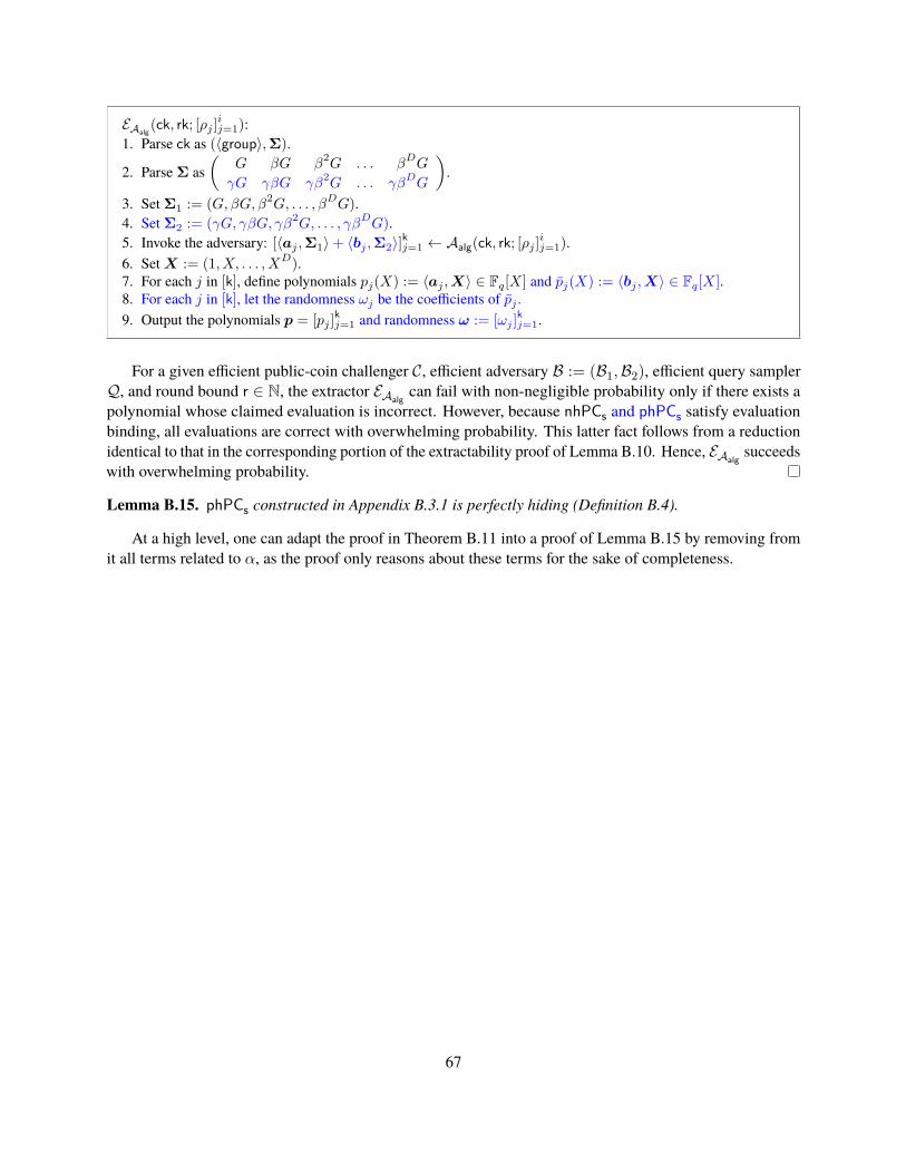
EAalg(ck, rk; [ρj ]
ij=1):
1. Parse ck as (〈group〉,Σ).
2. Parse Σ as(
G βG β2G . . . βDG
γG γβG γβ2G . . . γβDG
).
3. Set Σ1 := (G, βG, β2G, . . . , βDG).4. Set Σ2 := (γG, γβG, γβ2G, . . . , γβDG).5. Invoke the adversary: [〈aj ,Σ1〉+ 〈bj ,Σ2〉]
kj=1 ← Aalg(ck, rk; [ρj ]
ij=1).
6. SetX := (1, X, . . . ,XD).7. For each j in [k], define polynomials pj(X) := 〈aj ,X〉 ∈ Fq[X] and pj(X) := 〈bj ,X〉 ∈ Fq[X].8. For each j in [k], let the randomness ωj be the coefficients of pj .9. Output the polynomials p = [pj ]
kj=1 and randomness ω := [ωj ]
kj=1.
For a given efficient public-coin challenger C, efficient adversary B := (B1,B2), efficient query samplerQ, and round bound r ∈ N, the extractor EAalg
can fail with non-negligible probability only if there exists apolynomial whose claimed evaluation is incorrect. However, because nhPCs and phPCs satisfy evaluationbinding, all evaluations are correct with overwhelming probability. This latter fact follows from a reductionidentical to that in the corresponding portion of the extractability proof of Lemma B.10. Hence, EAalg
succeedswith overwhelming probability.
Lemma B.15. phPCs constructed in Appendix B.3.1 is perfectly hiding (Definition B.4).
At a high level, one can adapt the proof in Theorem B.11 into a proof of Lemma B.15 by removing fromit all terms related to α, as the proof only reasons about these terms for the sake of completeness.
67

C Polynomial commitments for multiple degree bounds
We construct a polynomial commitment scheme that supports multiple degree bounds up to a maximumdegree chosen at setup time.
We again temporarily restrict our attention to the case where, in the reveal phase, all polynomials areevaluated at the same evaluation point. (We will relax this restriction in Appendix D.) We do not provide astandalone definition for the construction that we consider below, because it equals the definition in Section 6.1when restricted to admissible query samplers which output query sets Q consisting of a single evaluationpoint at which a subset of the polynomials are evaluated (i.e., Q = T × z for some T ⊆ [n], and z ∈ F).14
We proceed as follows. First, in Appendix C.1, we present a construction for the above goal that buildsupon ideas in Appendix B.3.1. Then, in Appendix C.2, we reduce the hiding and extractability of thisconstruction to the hiding and extractability of a related construction that is simpler to analyze, but is notdegree-efficient. This simpler construction might also be of independent interest.
C.1 Degree-efficient construction
We demonstrate how to construct a polynomial commitment that supports multiple degree bounds efficiently.Our construction builds upon the construction in Appendix B.3.1. A polynomial commitment schemeover a field family F for multiple degree bounds and a single evaluation point is a tuple of algorithmsPCm = (Setup,Trim,Commit,Open,Check) with the following syntax. Below we use [[ai, bi]]
ni=1 as a
short-hand for the tuple (a1, b1, . . . , an, bn). The highlighted text below denotes the parts of the constructionthat differ from the construction in Appendix B.3.1.Setup. On input a security parameter λ (in unary), and a maximum degree bound D ∈ N, PCm.Setupsamples public parameters pp as follows. Sample a bilinear group 〈group〉 ← SampleGrp(1λ), and parse〈group〉 as a tuple (G1,G2,GT , q, G,H, e). Sample random elements β, γ ∈ Fq. Then compute the vector
Σ :=
(G βG β2G . . . βDG
γG γβG γβ2G . . . γβDG
)∈ G2D+2
1 .
Set pp := (D, 〈group〉,Σ, βH), and then output the public parameters pp. These public parameters willsupport polynomials over the field Fq of degree at most D.Trim. Given oracle access to public parameters pp, and on input a security parameter λ (in unary), anddegree bounds d = [di]
ni=1, PCm.Trim
pp deterministically computes a key pair (ck, rk) that is specialized tod as follows. Let d be the maximum degree bound in d. Then obtain Σck from public parameters:
Σck :=
(G βG . . . βdG βD−dG βD−d+1G . . . βDG
γG γβG . . . γβdG
)∈ G3d+3
1 .
Set ck := (Σck,d). Let Σrk be the set βD−diGi∈[n] and rk := (D, 〈group〉,Σrk, γG, βH,d), and then
output the key pair (ck, rk). This key pair is specialized to d.Commit. On input ck, univariate polynomials p = [pi]
ni=1 over the field Fq, degree bounds d = [di]
ni=1 with
deg(p) ≤ d ≤ D, and randomness ω = [[ωi, ω′i]]ni=1, PCm.Commit outputs commitments c = [ci]
ni=1 that
are computed as follows. Obtain the supported degree bounds d′ from ck. If for any pi ∈ p, deg(pi) > di
14Recall from Definition 6.5 that an admissible query sampler outputs query sets such that every polynomial is evaluated at leastonce at a point sampled from a super-polynomially-large subset.
68

or di 6∈ d′, abort. For each i ∈ [n], if ωi and ω
′i are not ⊥, then obtain from them random univariate
polynomials pi and p′i of degree deg(pi); otherwise, set pi and p
′i to be the zero polynomial. For each i ∈ [n],
compute ci := pi(β)G + γpi(β)G and c′i := βD−dipi(β)G + γp′i(β)G. Finally, set ci := (ci, c′i), and
output c := [ci]ni=1. Note that because pi(X), XD−dipi(X), pi(X) and p′i(X) have at most di non-zero
coefficients, the above terms are linear combinations of terms in ck.Open. On input ck, univariate polynomials p = [pi]
ni=1 over the field Fq, degree bounds d = [di]
ni=1,
evaluation point z ∈ Fq, opening challenge ξ, and randomness ω = [[ωi, ω′i]]ni=1, PCm.Open outputs the
evaluation proof π as follows. Obtain the supported degree bounds d′ from ck. If for any pi ∈ p, deg(pi) > dior di 6∈ d
′, abort. For each i ∈ [n], if ωi and ω′i are not ⊥, obtain from them random univariate polynomials
pi and p′i of degree deg(pi); otherwise, set pi and p
′i to be the zero polynomial.
Then, for each i ∈ [n], define the polynomial p?i (X) := XD−dipi(X) −XD−dipi(z), and compute awitness polynomial for wi(X) := pi(X)−pi(z)
X−z for pi, and a witness polynomial w?i (X) := XD−diwi(X) forp?i . Finally, compute the witness polynomial for these 2n polynomials as w :=
∑ni=1 ξ
iwi +∑n
i=1 ξn+iw?i .
Next, compute the linear combination of the random polynomials p :=∑n
i=1 ξipi and p
′ :=∑n
i=1 ξn+ip′i,
and compute thewitness polynomial w(X) := p(X)−p(z)+p′(X)−p′(z)X−z for these. Setw := w(β)G+γw(β)G ∈
G1, and v := p(z) + p′(z) ∈ Fq. The evaluation proof is π := (w, v).Check. On input rk, commitments c = [ci]
ni=1, degree bounds d = [di]
ni=1, evaluation point z ∈ Fq, alleged
evaluations v = [vi]ni=1, evaluation proof π = (w, v), and opening challenge ξ, PCm.Check proceeds as
follows. Obtain the supported degree bound d′ from rk. If for any di ∈ d, di 6∈ d′, abort. Parse each
commitment ci as a pair of sub-commitments (ci, c′i), and construct c
?i := c
′i − viβ
D−diG. Next, computethe two linear combinations
C :=n∑i=1
ξici +n∑i=1
ξn+ic?i , v :=
n∑i=1
ξivi,
Then check the evaluation proof π = (w, v) via the equality e(C − vG− γvG,H) = e(w, βH − zH).
Lemma C.1. The scheme PCm constructed above achieves completeness (Definition 6.1).
Proof. Fix any maximum degree bounds D, d = [di]ni=1 and efficient adversary A. Let pp be any public
parameters output by the algorithm PCm.Setup(1λ, D). Let A(pp) select polynomials p = [pi]ni=1 over Fq,
degree bounds d = [di]ni=1, location z ∈ Fq, and opening challenge ξ ∈ Fq. We only need to consider
adversaries A that make choices for which deg(p) ≤ di ≤ D. Let (ck, rk) be any key pair output by thealgorithm PCm.Trim
pp(1λ,d) constructed above. The keys contain a description 〈group〉 of a bilinear groupof some prime order q, which in particular induces a field Fq.
Now consider commitments c = [ci]ni=1 and evaluation proof π that are all computed according to the
construction above. We need to show that, for the correct evaluations v := p(z),
PCm.Check(rk, c,d, z,v, π, ξ) = 1 .
This amounts to arguing that the pairing equations are satisfied. For these equations, note that the combinedcommitment C and evaluation v are computed by PCm.Check as follows:
69

C =n∑i=1
ξici +n∑i=1
ξn+ic?i
=n∑i=1
ξi(pi(β)G+ γpi(β)G) +n∑i=1
ξn+i(βD−di(pi(β)− pi(z))G+ γp′i(β)G)
=n∑i=1
ξi(pi(β)G+ γpi(β)G) +n∑i=1
ξn+i(p?i (β)G+ γp′i(β)G) ,
v =n∑i=1
ξivi =n∑i=1
ξipi(z) .
In the evaluation proof π = (w, v), we have that
w = (w(β) + γw(β))G
=
n∑i=1
ξiwi(β)G+
n∑i=1
ξn+iw?i (β)G+
n∑i=1
ξiwi(β)γG+
n∑i=1
ξn+iw′i(β)γG
=
n∑i=1
ξi(pi(β)− pi(z)) + ξn+ip?i (β) + ξi(pi(β)− pi(z))γ + ξn+i(p′i(β)− p′i(z))γβ − z
G
We also have that the evaluation v = p(z) + p′(z). Therefore,
e(C − vG− γvG,H)
= e(∑n
i=1(ξi((pi(β)− vi) + γ(pi(β)− pi(z))) + ξn+i(p?i (β) + γ(p′i(β)− p′i(z))))G,H)
= e(∑n
i=1 ξi(pi(β)−pi(z))+ξ
n+ip?i (β)+ξ
i(pi(β)−pi(z))γ+ξ
n+i(p
′i(β)−p′i(z))γ
β−z G, (β − z)H)
= e((w(β) + γw(β))G, βH − zH)
= e(w, βH − zH) .
We conclude that the pairing equation also holds.
Lemma C.2. The scheme PCm constructed achieves efficiency, as defined in Definition 6.3.
Proof. PCm satisfies both efficiency properties:• Degree-efficiency: For a list of n polynomials with degree bounds d = [di]
ni=1 where d = max(d) is the
maximum supported degree bounds for these polynomials, both PCm.Commit and PCm.Open only handlepolynomials having at most d coefficients, and so the time to commit to the polynomials is the time for4n variable-base multi-scalar multiplications of size at most d, while the time to compute an evaluationproof is the time to compute two polynomial divisions of degree at most d plus the time required for twovariable-base multi-scalar multiplications of size at most d.
• Succinctness: For a list of n polynomials, the scheme PCm requires 2n G1 elements for a commitment andone G1 element and one Fq element for an evaluation proof, while the time to check this proof requires twovariable-base multi-scalar multiplications of size n and two pairings.
Extractability and hiding. We reduce the extractability and hiding properties of our construction to thoseof a simpler-to-analyze construction described below. This latter construction makes black-box use of anyPCs scheme.
70

C.2 Black-box construction
We now provide a simpler construction of PCm that makes black-box use of PCs. This construction is notdegree-efficient (Definition 6.3), but is simpler to analyze.Setup. On input a security parameter λ (in unary), and a maximum degree bound D ∈ N, PCm.Setupsamples and outputs pp := PCs.Setup(1λ, D). The keys contain the description of a finite field F ∈ F .Trim. Given oracle access to public parameters pp, and on input a security parameter λ (in unary), anddegree bounds d, PCm.Trim simply parses pp as (ck, rk) and outputs these.Commit. On input ck, univariate polynomials p = [pi]
ni=1 over the field F, degree bounds d = [di]
ni=1
with deg(p) ≤ d ≤ D, and randomness ω = [[ωi, ω′i]]ni=1, PCm.Commit outputs commitments c = [ci]
ni=1
that are computed as follows. First, for each i ∈ [n], define the shifted polynomial p′i(X) := XD−dipi(X).Next, use PCs to simultaneously commit to all unshifted and shifted polynomials: [[ci, c
′i]]ni=1 :=
PCs.Commit(ck, [[pi, p′i]]ni=1;ω). Finally, set ci := (ci, c
′i), and output c := [ci]
ni=1. Note that every
polynomial being committed has degree at most D.Open. On input ck, univariate polynomials p = [pi]
ni=1 over the field F, degree bounds d = [di]
ni=1,
evaluation point z ∈ F, opening challenge ξ, and randomness ω = [[ωi, ω′i]]ni=1, PCm.Open outputs the
evaluation proof π := PCs.Open(ck, [[pi, p′i]]ni=1, z, ξ;ω), where each p′i is the shift of pi respectively.
Check. On input rk, commitments c = [ci]ni=1, degree bounds d = [di]
ni=1, evaluation point z ∈ F, alleged
evaluations v = [vi]ni=1, evaluation proof π, and opening challenge ξ, PCm.Check proceeds as follows. Parse
each commitment ci as a pair of sub-commitments (ci, c′i). For each i ∈ [n], compute the shifted evaluation
v′i := zD−divi. Check that PCs.Check(rk, [[ci, c′i]]ni=1, z, [[vi, v
′i]]ni=1, π, ξ) accepts.
Lemma C.3. If PCs achieves completeness (Definition B.1) then PCm achieves completeness (Definition 6.1).
Proof. If an adversary A(ck, rk) selects polynomials [pi]ni=1, degree bounds [di]
ni=1, evaluation point z ∈ F,
and opening challenge ξ such that, for every i ∈ [n], we have deg(pi) ≤ di ≤ D, then both the unshiftedpolynomials [pi]
ni=1 and shifted polynomials [p′i]
ni=1 have degree at most D. Furthermore, because the
shifted polynomials are computed as p′(X) = XD−dip(X), the shifted evaluations will always match:v′i = zD−di · vi. This means that the completeness of PCs ensures that the commitments produced via PCs
will pass the tests in PCs.Check.
Lemma C.4. If PCs achieves succinctness (Definition B.3) then PCm achieves succinctness (Definition 6.3).
Proof. The commitment of PCm contains 2n PCs commitments and the evaluation proof contains one PCs
proof. The time to check n evaluations is the same as the time to check 2n evaluations in PCs, plus at mostn · (logD) field operations to compute v′.
Lemma C.5. If the construction in Appendix C.2 achieves extractability and hiding when instantiated withPCs from Appendix B.3, then so does the construction in Appendix C.1.
Proof. We show how to reduce the extractability and hiding of the construction in Appendix C.1 (denoted byPCm) to that of the foregoing construction (denoted by PC
′m). For simplicity, we consider the case of a single
polynomial p with a single degree bound d evaluated at the query point z.• Extractability: Note that PCm commitments are identical to PC′m commitments. The same holds forevaluation proofs for unshifted polynomials. Hence, the only difference is in how degree bounds areenforced, and so we focus on this latter aspect.
71

Define the polynomials p1 := XD−dp(X)−XD−dv and p2 := XD−dp(X). To enforce degree bounds,PCm provides an evaluation proof for the claim that p1(z) = 0, while PC′m provides a proof for theclaim that p2(z) = zD−dv. However, notice that p2(z) = zD−dv if and only if p2(z) = 0, and so a PCm
evaluation proof is valid only if the “corresponding” PC′m proof is also valid.• Hiding: Note that PCm commitments and evaluation proofs for unshifted polynomials are identical to thosefor PC′m, and so we focus on evaluation proofs for shifted polynomials. As seen from the calculation ofPCm, the witness polynomial for p1 is a shifted version of the witness polynomial for p, and hence theevaluation proof does not reveal any additional information about p.
C.2.1 Extractability
Theorem C.6. If PCs achieves extractability (Definition B.2) then PCm achieves extractability (Definition 6.2restricted to query sets Q querying a subset of polynomials at the same point (i.e., Q = T × z for someT ⊆ [n], and z ∈ F).
Proof. Fix a maximum degree boundD and an efficient adversary A against PCm. We use A to construct anadversary B and query sampler Q′ against PCs. By assumption there exists a PCs extractor EB against B. Weuse EB to construct an PCm extractor EA for A.
B(ck, rk, [ρj ]ij=1):
1. Set pp := (ck, rk).2. Compute (c,d)← A(pp, [ρj ]
ij=1).
3. Parse c as [[ci, c′i]]ni=1.
4. Output [[ci, c′i]]ni=1.
EA(pp, [ρj ]ij=1):
1. Parse pp as (ck, rk).2. Compute p← EB(ck, rk, [ρj ]
ij=1).
3. Parse p as [[pi, p′i]]ni=1.
4. Output [pi]ni=1.
Suppose for contradiction that the extractor EA fails with non-negligible probability for some choice ofround bound r ∈ N, efficient public-coin challenger C, efficient query sampler Q, and efficient adversaryB = (B1,B2). This can occur due to one of two reasons.(1) Extracted polynomial does not match evaluation: there exists an extracted polynomial whose claimed
evaluation is incorrect.(2) Degree bounds are not satisfied: all extracted polynomials match their claimed evaluations, but there
exists a polynomial whose degree differs from the claimed degree.If EA fails with non-negligible probability, then one of these cases occurs with non-negligible probability. Weanalyze both cases, and argue that this cannot be.(1) Extracted polynomial does not match evaluation. Each PCm commitment ci in [ci]i∈T is a pairof PCs commitments (ci, c
′i). Since PCm.Check invokes PCs.Check, [ci]i∈T are accepted by PCm.Check
if and only if [[ci, c′i]]i∈T are accepted by PCs.Check. Thus, if PCm.Check accepts but the extractor
EA fails with non-negligible probability, then we deduce that PCs.Check accepts but the extractor EBfails with non-negligible probability against a PCs query sampler Q′ that obtains Q from Q and outputsQ′ := (2i− 1, z), (2i, z) | (i, z) ∈ Q. This contradicts the fact that PCs achieves extractability. Hence,we conclude that all extracted polynomials match their claimed evaluations with probability negligibly closeto 1.(2) Degree bounds are not satisfied. We first recall how the extractor EA works: it invokes the PCs
extractor to obtain 2n polynomials p := [pi, p′i]ni=1, and outputs [pi]
ni=1. The remaining polynomials [p′i]
ni=1
72

are supposedly “shifted” versions of the output polynomials. It should be the case that for each i ∈ T itholds that p′i(X) = XD−dipi(X). To check that this condition is satisfied, PCm.Check verifies that, fora point z ∈ F sampled by the admissible query sampler Q, v′i := zD−dipi(z) is a valid evaluation for p′i.The probability that this equation holds but p′i(X) 6= XD−dipi(X) is negligibly small because Q, beingadmissible, samples z from a super-polynomially-large subset of F.
C.2.2 Hiding
Theorem C.7. If PCs achieves hiding (Definition B.4) then PCm achieves hiding (Definition 6.4 restricted toquery sets Qj querying a subset of polynomials at the same point (i.e., Qj = Tj × zj for some Tj ⊆ [n],and zj ∈ F).
Proof. Below we construct a simulator Sm for PCm using a simulator Ss for PCs as a subroutine.
Sm.Setup(1λ, D):1. Compute (ck, rk, trap)← Ss.Setup(1λ, D).2. Output (pp := (ck, rk), trap).
Sm.Commit(trap,d;ω):1. Ignore the degrees d, and parse the randomness ω as [[ωi, ω
′i]]
ki=1.
2. Compute [[ci, c′i]]
ki=1 := Ss.Commit(trap, 2k; [[ωi, ω
′i]]
ki=1).
3. For each i ∈ [k], assemble the pair ci := (ci, c′i) of simulated commitments.
4. Output the simulated commitments c := [ci]ni=1 for PCm.
Sm.Open(trap,p,v,d, Q, ξ;ω):1. Parse p,v,d,ω as [pi]
ni=1, [vi]
ni=1, [di]
ni=1, [[ωi, ω
′i]]ni=1.
2. Parse Q as T × z for some T ⊆ [n] and z ∈ F.3. For each i ∈ T , set p′i(X) := XD−dipi(X) and v′i := zD−divi.4. Construct PCs query set Q
′ := (2i− 1, z), (2i, z) | (i, z) ∈ Q.5. Output π ← Ss.Open(trap, [pi, p
′i]ni=1, [vi, v
′i]ni=1, Q
′, ξ; [[ωi, ω′i]]ni=1).
The simulator Sm is a simple wrapper around the simulator Ss, and it is straightforward to see that if Sssimulates correctly for PCs then Sm simulates correctly for PCm.
73

D Polynomial commitments that support different query locations
We construct a polynomial commitment scheme PC that supports different query locations–an instantiationof the primitive defined in Section 6.1. The query set Q consists of tuples (i, z) ∈ [n]× Fq of polynomialindices and evaluation points. The construction is again a black-box extension of the polynomial commitmentscheme PCm considered in Appendix C which only supports a single query.
D.1 Construction
PC.Setup, PC.Trim, and PC.Commit equal PCm.Setup, PCm.Trim, and PCm.Commit in Appendix C, andso below we show how to construct PC.Open and PC.Check.Open. On input ck, univariate polynomials p over the field F, degree bounds d, the query set Q, openingchallenge ξ, and randomness ω that is the same one used in PC.Commit, PC.Open proceeds as follows.Suppose there are t different evaluation points [zi]
ti=1 in the query set Q. Divide p into different (possibly
overlapping) groups [pi]ti=1, where every polynomial in pi is evaluated at point zi according to Q. Similarly
divide degree bounds d and ω as [di]ti=1 and [ωi]
ti=1 so that deg(pi) ≤ di and ωi is the randomness for the
polynomial pi. For each group pi, obtain the evaluation proof πi := PCm.Open(ck,pi,di, zi, ξ;ωi). Outputall the proofs of evaluation [πi]
ti=1.
Check. On input rk, commitments c, degree bounds d, the query set Q, alleged evaluations v, evaluationproof π, and opening challenge ξ, PC.Check proceeds as follows. Suppose there are t different evaluationpoints [zi]
ti=1 in the query set Q. Parse c, d, v and π as [ci]
ti=1, [di]
ti=1, [vi]
ti=1 and [πi]
ti=1 so that ci are the
commitments of polynomials pi, where deg(pi) ≤ di and pi(zi) is supposed to be vi. For each i ∈ [t], checkthat PCm.Check(rk, ci,di, zi,vi, πi, ξ) accepts.
Completeness. The completeness of PC follows directly from the completeness of PCm.Efficiency. PC satisfies both efficiency properties defined in Definition 6.3:• Degree efficiency: The degree efficiency of PC follows directly from the degree efficiency of PCm, becausePC.Commit is the same as PCm.Commit, and PC.Open invokes PCm.Open a total of t = |Q|.
• Succinctness: The succinctness of PC follows directly from the succinctness of PCm. In particular, a PCcommitment equals a PCm commitment, and is hence of size poly(λ). Similarly, a PC evaluation proofconsists of t PCm evaluation proofs, and is hence of size t · poly(λ) = poly(λ). Finally, PC.Check invokesPCm.Check t times such that the i-th invocation is over |ci| commitments. Because PCm.Check takes timen · poly(λ) to check n commitments, PC.Check takes time
∑ti=1 |ci| · poly(λ).
D.2 Extractability
Theorem D.1. If PCm in Appendix C achieves extractability (Definition 6.2) then PC also achievesextractability (Definition 6.2).
Proof. Suppose for contradiction that there exists a maximum degree bound D ∈ N and efficient adversaryA against PC such that for some choice of round bound r ∈ N, efficient public-coin challenger C, efficientquery sampler Q, and efficient adversary B = (B1,B2), every efficient extractor EA fails with non-negligibleprobability µ(λ).
Then, we show how to use these to break extractability for PCm by constructing adversary A′, querysampler Q′, and adversary B′ as follows. We define A′ to equal A, and construct Q′ and B′ below.
74

Q′(pp, [ρj ]rj=1) :
1. Obtain query set Q← Q(pp, [ρj ]rj=1).
2. Parse Q as ∪j∈[t]Tj × zj, for some Tj ⊆ [n] and zj ∈ F, whereeach zj is distinct.
3. Uniformly sample k ∈ [t].4. Output Q′ := Tk × zk.
B′1(pp, [ρj ]rj=1, Q) :
1. Parse Q as (i, z) | i ∈ [n] for some z ∈ F.2. Obtain query set QPC ← Q(pp, [ρj ]
rj=1).
3. Parse QPC as ∪j∈[t]Tj × zj, for some Tj ⊆ [n] and zj ∈ F, whereeach zj is distinct.
4. Check that for some k ∈ [t], Q = Qk.5. Obtain (v, stPC)← B1(pp, [ρj ]
rj=1, QPC).
6. Parse v as [vi]ti=1 similarly to above.
7. Output (vk, st := (stPC, k)).
B′2(st, ξ) :1. Parse st as (stPC, k).2. Obtain proof π ← B2(stPC, ξ).3. Parse π as [πj ]
tj=1.
4. Output πk .
Now, by assumption, there exists an extractor EA′ for PCm that succeeds in extracting against any choice ofQ′ and B′. In particular, it succeeds against Q′ and B′ constructed above. Because the extractor EA := EA′
fails only if EA′ fails, we need only to analyze the probability with which this latter algorithm fails. We knowthat whenever EA fails, PC.Check accepts, but there exists k ∈ [t] such that
deg(pk) 6≤ dk ∨ vk 6= pk(zk) .
By construction of PC.Check, this means that the k-th invocation of PCm.Check succeeds, but the corre-sponding polynomials are either of incorrect degree or have incorrect claimed evaluations. BecauseQ′ selectsthis index k with probability 1/t, A′ and B′ break extractability of PCm with non-negligible probabilityµ(λ)/t, thus contradicting our assumption.
D.3 Hiding
Theorem D.2. If PCm in Appendix C achieves hiding (Definition 6.4) then PC also achieves hiding(Definition 6.4).
Proof. We achieve this by constructing a simulator SPC for PC using the PCm simulator Sm. SPC.Setup,SPC.Trim, and SPC.Commit are the same as Sm.Setup, Sm.Trim, and Sm.Commit, and so we focus onconstructing SPC.Open.
75

SPC.Open(trap,p,v,d, Qi, ξi;ω):1. Parse Q as ∪i∈[t]Tj × zi, for some Ti ⊆ [n] and zi ∈ F, where each zi is distinct.2. Divide p, d, and ω into [pi]
ti=1, [di]
ti=1, and [ωi]
ti=1 so that pi = [pj ]j∈Ti
, di = [dj ]j∈Ti, and ωi = [ωj ]j∈Ti
.3. For each i in 1, . . . , t, compute evaluation proof πi ← Sm.Open(trap,pi,vi, Qi := Ti × zi, ξ;ωi).4. Output πi := [πi]
ti=1.
The simulator SPC is a simple wrapper around the simulator Sm. Since Sm achieves perfect hiding, so doesSPC regardless of τ , the number of query sets Qi, or ti, the respective number of distinct points in each queryset.
76

AcknowledgmentsThis research was supported by: an Engineering and Physical Sciences Research Council grant (EP/N028104/1), aGoogle Faculty Award, the RISELab at UC Berkeley, and donations from the Ethereum Foundation and the InterchainFoundation. The authors thank Dev Ojha and Nicholas Spooner for identifying and helping to fix an error in a priorversion of our AHP for the lincheck problem (Fig. 4).
References[Abd+19] B.Abdolmaleki, K.Baghery,H. Lipmaa, J. Siim, andM.Zajac. “UC-SecureCRSGeneration for SNARKs”.
In: Proceedings of the 11th International Conference on Cryptology in Africa. AFRICACRYPT ’19.2019, pp. 99–117.
[Ame+17] S. Ames, C. Hazay, Y. Ishai, and M. Venkitasubramaniam. “Ligero: Lightweight Sublinear ArgumentsWithout a Trusted Setup”. In: Proceedings of the 24th ACMConference on Computer and CommunicationsSecurity. CCS ’17. 2017, pp. 2087–2104.
[Aro+98] S. Arora, C. Lund, R. Motwani, M. Sudan, and M. Szegedy. “Proof verification and the hardness ofapproximation problems”. In: Journal of the ACM 45.3 (1998). Preliminary version in FOCS ’92.,pp. 501–555.
[AS98] S. Arora and S. Safra. “Probabilistic checking of proofs: a new characterization of NP”. In: Journal ofthe ACM 45.1 (1998). Preliminary version in FOCS ’92., pp. 70–122.
[Bab85] L. Babai. “Trading group theory for randomness”. In: Proceedings of the 17th Annual ACM Symposiumon Theory of Computing. STOC ’85. 1985, pp. 421–429.
[Bab+91] L. Babai, L. Fortnow, L. A. Levin, and M. Szegedy. “Checking computations in polylogarithmic time”. In:Proceedings of the 23rd Annual ACM Symposium on Theory of Computing. STOC ’91. 1991, pp. 21–32.
[BB04] D. Boneh and X. Boyen. “Short Signatures Without Random Oracles”. In: Proceedings of the 23rd AnnualInternational Conference on Theory and Application of Cryptographic Techniques. EUROCRYPT ’04.2004, pp. 56–73.
[BCC88] G. Brassard, D. Chaum, and C. Crépeau. “Minimum disclosure proofs of knowledge”. In: Journal ofComputer and System Sciences 37.2 (1988), pp. 156–189.
[BCS16] E. Ben-Sasson, A. Chiesa, and N. Spooner. “Interactive Oracle Proofs”. In: Proceedings of the 14thTheory of Cryptography Conference. TCC ’16-B. 2016, pp. 31–60.
[Ben+14a] E. Ben-Sasson, A. Chiesa, E. Tromer, and M. Virza. “Scalable Zero Knowledge via Cycles of EllipticCurves”. In: Proceedings of the 34th Annual International Cryptology Conference. CRYPTO ’14.Extended version at http://eprint.iacr.org/2014/595. 2014, pp. 276–294.
[Ben+14b] E. Ben-Sasson, A. Chiesa, E. Tromer, and M. Virza. “Succinct Non-Interactive Zero Knowledge fora von Neumann Architecture”. In: Proceedings of the 23rd USENIX Security Symposium. USENIXSecurity ’14. Extended version at http://eprint.iacr.org/2013/879. 2014, pp. 781–796.
[Ben+15] E. Ben-Sasson, A. Chiesa, M. Green, E. Tromer, and M. Virza. “Secure Sampling of Public Parametersfor Succinct Zero Knowledge Proofs”. In: Proceedings of the 36th IEEE Symposium on Security andPrivacy. S&P ’15. 2015, pp. 287–304.
[Ben+16] E. Ben-Sasson, A. Chiesa, A. Gabizon, and M. Virza. “Quasilinear-Size Zero Knowledge from Linear-Algebraic PCPs”. In: Proceedings of the 13th Theory of Cryptography Conference. TCC ’16-A. 2016,pp. 33–64.
[Ben+17a] E. Ben-Sasson, A. Chiesa, A. Gabizon, M. Riabzev, and N. Spooner. “Interactive Oracle Proofs withConstant Rate and Query Complexity”. In: Proceedings of the 44th International Colloquium on Automata,Languages and Programming. ICALP ’17. 2017, 40:1–40:15.
77
[Ben+17b] E. Ben-Sasson et al. “Computational integrity with a public random string from quasi-linear PCPs”. In:Proceedings of the 36th Annual International Conference on Theory and Application of CryptographicTechniques. EUROCRYPT ’17. 2017, pp. 551–579.
[Ben+19a] E. Ben-Sasson, I. Bentov, Y. Horesh, and M. Riabzev. “Scalable Zero Knowledge with No TrustedSetup”. In: Proceedings of the 39th Annual International Cryptology Conference. CRYPTO ’19. 2019,pp. 733–764.
[Ben+19b] E. Ben-Sasson, A. Chiesa, L. Goldberg, T. Gur, M. Riabzev, and N. Spooner. “Linear-Size Constant-QueryIOPs for Delegating Computation”. In: Proceedings of the 17th Theory of Cryptography Conference.TCC ’19. 2019.
[Ben+19c] E. Ben-Sasson, A. Chiesa, M. Riabzev, N. Spooner, M. Virza, and N. P. Ward. “Aurora: TransparentSuccinct Arguments for R1CS”. In: Proceedings of the 38th Annual International Conference on theTheory and Applications of Cryptographic Techniques. EUROCRYPT ’19. Full version available athttps://eprint.iacr.org/2018/828. 2019, pp. 103–128.
[BG04] D. R. L. Brown and R. P. Gallant. The Static Diffie–Hellman Problem. Cryptology ePrint Archive, Report2004/306. 2004.
[BG12] S. Bayer and J. Groth. “Efficient Zero-Knowledge Argument for Correctness of a Shuffle”. In: Proceedingsof the 31st Annual International Conference on Theory and Applications of Cryptographic Techniques.EUROCRYPT ’12. 2012, pp. 263–280.
[BGG17] S. Bowe, A. Gabizon, and M. Green. A multi-party protocol for constructing the public parameters of thePinocchio zk-SNARK. Cryptology ePrint Archive, Report 2017/602. 2017.
[BGM17] S. Bowe, A. Gabizon, and I. Miers. Scalable Multi-party Computation for zk-SNARK Parameters in theRandom Beacon Model. Cryptology ePrint Archive, Report 2017/1050. 2017.
[Bit+13] N. Bitansky, A. Chiesa, Y. Ishai, R. Ostrovsky, and O. Paneth. “Succinct Non-Interactive Arguments viaLinear Interactive Proofs”. In: Proceedings of the 10th Theory of Cryptography Conference. TCC ’13.2013, pp. 315–333.
[Bit+16] N. Bitansky, R. Canetti, O. Paneth, and A. Rosen. “On the Existence of Extractable One-Way Functions”.In: SIAM Journal on Computing 45.5 (2016). Preliminary version appeared in STOC ’14., pp. 1910–1952.
[Bon+17] D. Boneh, Y. Ishai, A. Sahai, and D. J. Wu. “Lattice-Based SNARGs and Their Application to MoreEfficient Obfuscation”. In: Proceedings of the 36th Annual International Conference on Theory andApplications of Cryptographic Techniques. EUROCRYPT ’17. 2017, pp. 247–277.
[Bon+18] D. Boneh, Y. Ishai, A. Sahai, and D. J. Wu. “Quasi-Optimal SNARGs via Linear Multi-Prover InteractiveProofs”. In: Proceedings of the 37th Annual International Conference on Theory and Application ofCryptographic Techniques. EUROCRYPT ’18. 2018, pp. 222–255.
[Boo+16] J. Bootle, A. Cerulli, P. Chaidos, J. Groth, and C. Petit. “Efficient Zero-Knowledge Arguments forArithmetic Circuits in the Discrete Log Setting”. In: Proceedings of the 35th Annual InternationalConference on Theory and Application of Cryptographic Techniques. EUROCRYPT ’16. 2016, pp. 327–357.
[BP15] E. Boyle and R. Pass. “Limits of Extractability Assumptions with Distributional Auxiliary Input”. In:Proceedings of the 21st International Conference on the Theory and Application of Cryptology andInformation Security. ASIACRYPT ’15. 2015, pp. 236–261.
[BS08] E. Ben-Sasson and M. Sudan. “Short PCPs with Polylog Query Complexity”. In: SIAM Journal onComputing 38.2 (2008). Preliminary version appeared in STOC ’05., pp. 551–607.
[Bün+18] B. Bünz, J. Bootle, D. Boneh, A. Poelstra, P. Wuille, and G. Maxwell. “Bulletproofs: Short Proofs forConfidential Transactions and More”. In: Proceedings of the 39th IEEE Symposium on Security andPrivacy. S&P ’18. 2018, pp. 315–334.
78

[CD98] R. Cramer and I. Damgård. “Zero-Knowledge Proofs for Finite Field Arithmetic; or: Can Zero-Knowledgebe for Free?” In: Proceedings of the 18th Annual International Cryptology Conference. CRYPTO ’98.1998, pp. 424–441.
[CFS17] A. Chiesa, M. A. Forbes, and N. Spooner. A Zero Knowledge Sumcheck and its Applications. CryptologyePrint Archive, Report 2017/305. 2017.
[Che10] J. H. Cheon. “Discrete Logarithm Problems with Auxiliary Inputs”. In: Journal of Cryptology 23.3(2010), pp. 457–476.
[Dan+14] G. Danezis, C. Fournet, J. Groth, and M. Kohlweiss. “Square Span Programs with Applications toSuccinct NIZK Arguments”. In: Proceedings of the 20th International Conference on the Theory andApplication of Cryptology and Information Security. ASIACRYPT ’14. 2014, pp. 532–550.
[Den02] A. W. Dent. “Adapting the Weaknesses of the Random Oracle Model to the Generic Group Model”.In: Proceedings of the 8th International Conference on the Theory and Application of Cryptology andInformation Security. ASIACRYPT ’02. 2002, pp. 100–109.
[FKL18] G. Fuchsbauer, E. Kiltz, and J. Loss. “The Algebraic Group Model and its Applications”. In: Proceedingsof the 38th Annual International Cryptology Conference. CRYPTO ’18. 2018, pp. 33–62.
[FS86] A. Fiat and A. Shamir. “How to prove yourself: practical solutions to identification and signatureproblems”. In: Proceedings of the 6th Annual International Cryptology Conference. CRYPTO ’86. 1986,pp. 186–194.
[Gab19] A. Gabizon. Improved prover efficiency and SRS size in a Sonic-like system. Cryptology ePrint Archive,Report 2019/601. 2019.
[Gen+13] R. Gennaro, C. Gentry, B. Parno, and M. Raykova. “Quadratic Span Programs and Succinct NIZKswithout PCPs”. In: Proceedings of the 32nd Annual International Conference on Theory and Applicationof Cryptographic Techniques. EUROCRYPT ’13. 2013, pp. 626–645.
[GKR15] S. Goldwasser, Y. T. Kalai, and G. N. Rothblum. “Delegating Computation: Interactive Proofs forMuggles”. In: Journal of the ACM 62.4 (2015), 27:1–27:64.
[GMR89] S. Goldwasser, S. Micali, and C. Rackoff. “The knowledge complexity of interactive proof systems”. In:SIAM Journal on Computing 18.1 (1989). Preliminary version appeared in STOC ’85., pp. 186–208.
[Gro10] J. Groth. “Short Pairing-Based Non-interactive Zero-Knowledge Arguments”. In: Proceedings of the16th International Conference on the Theory and Application of Cryptology and Information Security.ASIACRYPT ’10. 2010, pp. 321–340.
[Gro16] J. Groth. “On the Size of Pairing-Based Non-interactive Arguments”. In: Proceedings of the 35th AnnualInternational Conference on Theory and Applications of Cryptographic Techniques. EUROCRYPT ’16.2016, pp. 305–326.
[Gro+18] J. Groth, M. Kohlweiss, M. Maller, S. Meiklejohn, and I. Miers. “Updatable and Universal CommonReference Strings with Applications to zk-SNARKs”. In: Proceedings of the 38th Annual InternationalCryptology Conference. CRYPTO ’18. 2018, pp. 698–728.
[GWC19] A. Gabizon, Z. J. Williamson, and O. Ciobotaru. PLONK: Permutations over Lagrange-bases forOecumenical Noninteractive arguments of Knowledge. Cryptology ePrint Archive, Report 2019/953.2019.
[Kil92] J. Kilian. “A note on efficient zero-knowledge proofs and arguments”. In: Proceedings of the 24th AnnualACM Symposium on Theory of Computing. STOC ’92. 1992, pp. 723–732.
[KKM07] S. Kozaki, T. Kutsuma, and K. Matsuo. “Remarks on Cheon’s Algorithms for Pairing-Related Problems”.In: Proceedings of the 1st International Conference on Pairing-Based Cryptography. Pairing ’07. 2007,pp. 302–316.
79

[KZG10] A. Kate, G. M. Zaverucha, and I. Goldberg. “Constant-Size Commitments to Polynomials and TheirApplications”. In: Proceedings of the 16th International Conference on the Theory and Application ofCryptology and Information Security. ASIACRYPT ’10. 2010, pp. 177–194.
[Lip12] H. Lipmaa. “Progression-Free Sets and Sublinear Pairing-Based Non-Interactive Zero-KnowledgeArguments”. In: Proceedings of the 9th Theory of Cryptography Conference on Theory of Cryptography.TCC ’12. 2012, pp. 169–189.
[Mal+19] M. Maller, S. Bowe, M. Kohlweiss, and S. Meiklejohn. Sonic: Zero-Knowledge SNARKs from Linear-SizeUniversal and Updateable Structured Reference Strings. 2019.
[Mau05] U. M. Maurer. “Abstract Models of Computation in Cryptography”. In: Proceedings of the 10th IMAInternational Conference on Cryptography and Coding. IMA ’05. 2005, pp. 1–12.
[PST13] C. Papamanthou, E. Shi, and R. Tamassia. “Signatures of Correct Computation”. In: Proceedings of the10th Theory of Cryptography Conference. TCC ’13. 2013, pp. 222–242.
[PV05] P. Paillier and D. Vergnaud. “Discrete-Log-Based Signatures May Not Be Equivalent to Discrete Log”.In: Proceedings of the 11th International Conference on the Theory and Application of Cryptology andInformation Security. ASIACRYPT ’05. 2005, pp. 1–20.
[RRR16] O. Reingold, R. Rothblum, and G. Rothblum. “Constant-Round Interactive Proofs for DelegatingComputation”. In: Proceedings of the 48th ACM Symposium on the Theory of Computing. STOC ’16.2016, pp. 49–62.
[Set19] S. Setty. Spartan: Efficient and general-purpose zkSNARKs without trusted setup. Cryptology ePrintArchive, Report 2019/550. 2019.
[Sho97] V. Shoup. “Lower bounds for discrete logarithms and related problems”. In: Proceedings of the 16thInternational Conference on the Theory and Application of Cryptographic Techniques. EUROCRYPT ’97.1997, pp. 256–266.
[The] The Zcash Ceremony. https://z.cash/blog/the-design-of-the-ceremony.html. 2016.[Wah+18] R. S. Wahby, I. Tzialla, A. Shelat, J. Thaler, and M. Walfish. “Doubly-Efficient zkSNARKs Without
Trusted Setup”. In: Proceedings of the 39th IEEE Symposium on Security and Privacy. S&P ’18. 2018,pp. 926–943.
[Xie+19] T. Xie, J. Zhang, Y. Zhang, C. Papamanthou, and D. Song. “Libra: Succinct Zero-Knowledge Proofs withOptimal Prover Computation”. In: Proceedings of the 39th Annual International Cryptology Conference.CRYPTO ’19. 2019, pp. 733–764.
[Zca] Zcash. https://z.cash/. 2014.[Zha+17a] Y. Zhang, D. Genkin, J. Katz, D. Papadopoulos, and C. Papamanthou. A Zero-Knowledge Version of
vSQL. Cryptology ePrint Archive, Report 2017/1146. 2017.[Zha+17b] Y. Zhang, D. Genkin, J. Katz, D. Papadopoulos, and C. Papamanthou. “vSQL: Verifying Arbitrary SQL
Queries over Dynamic Outsourced Databases”. In: Proceedings of the 38th IEEE Symposium on Securityand Privacy. S&P ’17. 2017, pp. 863–880.
[Zha+18] Y. Zhang, D. Genkin, J. Katz, D. Papadopoulos, and C. Papamanthou. “vRAM: Faster Verifiable RAMwith Program-Independent Preprocessing”. In: Proceedings of the 39th IEEE Symposium on Securityand Privacy. S&P ’18. 2018, pp. 908–925.
80


![HW12,Math121A Spring,2004 UCBERKELEY · 2018-10-28 · HW12,Math121A Spring,2004 UCBERKELEY NasserM.Abbasi Spring,2004 CompiledonOctober28,2018at4:43pm [public] Contents 1 chapter15,problem4.12](https://img.dokumen.tips/doc/110x75/5f498e29df53537153674b1a/hw12math121a-spring2004-ucberkeley-2018-10-28-hw12math121a-spring2004-ucberkeley.jpg)